The κ Factor: Inferring Protocol Performance UsingInter-link Reception Correlation

Kannan Srinivasan†, Mayank Jain†, Jung Il Choi†, Tahir Azim†,Edward S Kim∗, Philip Levis†, and Bhaskar Krishnamachari∗

{srikank, mayjain, jungilchoi, tazim}@stanford.edu,e.skim@usc.edu, pal@cs.stanford.edu, bkrishna@usc.edu

†Stanford University ∗University of Southern CaliforniaStanford, CA-94305 Los Angeles, CA-90089

ABSTRACTThis paper explores metrics that capture to what degree packet re-ception on different links is correlated. Specifically, it exploresmetrics that shed light on when and why opportunistic routing andnetwork coding protocols perform well (or badly). It presents anew metric, κ that, unlike existing widely used metrics, has nobias based on the packet reception ratios of links. This lack of biasmakes κ a better predictor of performance of opportunistic routingand network coding protocols. Comparing Deluge and RatelessDeluge, Deluge’s network coding counterpart, we find that κ canpredict which of the two is best suited for a given environment. Forexample, irrespective of the packet reception ratios of the links, ifthe average κ of the link pairs is very high (close to 1.0), then us-ing a protocol that does not code works better than using a networkcoding protocol.

Measuring κ on several 802.15.4 and 802.11 testbeds, we findthat it varies significantly across network topologies and link layers.κ can be a metric for quantifying what kind of a network is presentand help decide which protocols to use for that network.

Categories and Subject Descriptors: C.2.1 [Network Architec-ture and Design]:Wireless communications

General Terms: Measurement, Design, Performance.

Keywords: 802.15.4, Wireless measurement study, Low powerwireless networks, Wireless protocol design.

1. INTRODUCTIONOne of the principal opportunities that wireless provides is the

ability to send a single packet to multiple receivers. Data dissemi-nation protocols such as Deluge [8] and broadcast protocols such asRBP [17] can broadcast data to multiple neighbors at once. Routingprotocols can snoop, or use opportunistic receptions [3], in order toforward packets even when delivery to the primary intended recip-ient fails.

In these schemes, correlations in packet reception on differentlinks can greatly impact protocol performance. For example, if all

Permission to make digital or hard copies of all or part of this work forpersonal or classroom use is granted without fee provided that copies arenot made or distributed for profit or commercial advantage and that copiesbear this notice and the full citation on the first page. To copy otherwise, torepublish, to post on servers or to redistribute to lists, requires prior specificpermission and/or a fee.MobiCom’10, September 20–24, 2010, Chicago, Illinois, USA.Copyright 2010 ACM 978-1-4503-0181-7/10/09 ...$10.00.

links receive the same packets (i.e their reception is completely cor-related,) then opportunistic routing protocols will not work betterthan the shortest path protocols, as there is no spatial diversity toexploit. At the other extreme, if the links are negatively correlated –a reception at one implies a failure at the other – then opportunisticrouting can be of great benefit.

In prior work, researchers have often concluded that packet re-ception on different links is largely independent [16, 15]. Miu et al.use the cross conditional measure, P (A = 0|B = 0)−P (A = 0),as a metric for inter-link correlation between links A and B [15].We refer to this metric as χ. χ tries to capture correlation in linklosses: if the losses on links A and B are independent then it’s zero.This metric was subsequently used by Reis et al. [16] and Lauferet al. [12] to conclude that most of the link pairs have independentpacket reception. Section 3 discusses properties desired of a cor-relation metric and shows that χ does not satisfy them: its valuedepends highly on the packet reception ratios (PRRs) of the twolinks. Section 5 further shows that χ is not indicative of how wellopportunistic routing protocols work.

Protocol designs typically assume that reception on different linksis independent [5, 7, 21, 12, 4, 10]. Network simulators [2, 13] andwork on network analysis also typically ignore these correlationsas it is commonly believed that these correlations are too hard tocapture.

From a set of wireless measurements over the past 4 years, wehave found that reception on different links is not always indepen-dent. This observation is not new; one of the earliest sensor net-work deployment studies, Great Duck Island, observed correlatedreception [18]. However, the degree of correlation varies greatlyacross network setups and link layers.

This paper presents a new metric called κ that captures this de-gree of correlation. κ is a 3-tuple metric that measures packet re-ception correlation on two links that have a common transmitter.A κ of 1 means that the receptions on the two links are highlycorrelated, zero means they are independent, and -1 means that thelosses on one are highly correlated with successes on the other. Un-like the existing metrics, the range of values that κ can take is nota function of PRRs of the links. This bias in other metrics makesthem poor estimators of protocol performance. Section 3 discussesthe κ metric in detail.

This paper shows that measuring correlation using κ can help usunderstand performance of protocols that exploit the broadcast na-ture of wireless to route or forward packets. Such protocols includeopportunistic and network coding protocols. This paper shows thatκ can predict opportunistic protocol performance. It shows how κcan be used to understand when a network coding protocol, such asRateless Deluge [7], is beneficial over protocols that don’t do net-

0 50 100 150Pkt #

0

2

4

6

8

10

12

14

Rece

iver

#

(a) Empirical Trace

0 50 100 150Pkt #

0

2

4

6

8

10

12

14

Rece

iver

#

(b) Synthetic Independent Trace

Figure 1: Packet reception at multiple receivers when a single transmitter is broadcasting packets; (a) empirical trace from Miragetestbed on channel 16, and (b) independent synthetic trace with same PRR. Packet losses are marked by black overlines. Theempirical trace has many more packet losses aligned across different receivers than the independent trace: empirical links (visually)show many correlated losses.

work coding. This allows researchers to make informed decisionsabout when to use network coding protocols for their testbeds anddeployments. Section 6 describes this comparison in detail. Sec-tions 4 and 5 systematically explore the usefulness of κ in under-standing opportunistic routing protocol performance.

Measuring κ on IEEE 802.15.4 [20] and 802.11 (WiFi) [1] net-works, we find that different networks see different degrees of cor-related link pairs. In one network nearly 70% of the link pairs havea κ higher than 0.8, while in another network less than 20% of thelink pairs fall in that range. This paper discusses possible causesof these correlations. In general, high power external interferencecauses packet losses at multiple receivers and increases correlation.Movement of an obstacle such that it blocks line-of-sight to onlyone receiver at a time reduces correlations. Section 7 investigatesand presents such factors that affect correlation.

Overall, this paper makes four research contributions. First, itoutlines desirable properties for an inter-link reception correlationmetric that can predict protocol performance. It shows that a widelyused metric does not satisfy these properties and is unsuitable forpredicting protocol performance. Second, it presents a new met-ric called κ that addresses the shortcomings of existing metrics.Third, it shows that κ explains how well an opportunistic proto-col like ExOR performs in a network. Fourth, it shows how κ canbe used to choose between network coding and no-network-codingprotocols for a network. Specifically, κ helps to choose the bestbetween Deluge and Rateless Deluge for a wireless network.

This paper shows that reception on different links can be cor-related and that measuring this correlation can help us understandwhen and why certain protocols perform the way they do. We be-lieve that this insight is useful in designing efficient future proto-cols.

2. TESTBEDSIn an attempt to observe and understand various degrees of cor-

relation present in wireless networks, this paper uses measurementsand experiments from both 802.15.4 [20] and 802.11b [1] networks.802.15.4 is an IEEE PHY-MAC low power, low data rate network

standard with a 16 channel spectrum that overlaps the spectrum of802.11b. It provides a data rate of 250 kbps and maximum transmitpower of 0dBm, which are much lower than 802.11b’s 11 Mbpscapability and 23dBm maximum transmit power.

We run 802.15.4 experiments using TinyOS running on the IntelMirage testbed [9], which consists of 100 Micaz [19] nodes placedalong the ceiling. An Ethernet back-channel provides communica-tion to all the nodes.

802.11b experiments run on a university testbed at data rates1, 2, 5.5 and 11 Mbps. We refer to this testbed as Universitytestbed. This testbed consists of 40 nodes located along the hall-ways of 2 adjacent department buildings in Stanford University.Packard Electrical Engineering Building houses 15 nodes specificto this network spread out across 4 floors. 25 nodes are located inGates Computer Science Building and are evenly distributed across6 floors. These nodes use the Madwifi driver and Click modularrouter [11] on a Linux kernel. Ethernet cables provide an IP basedback-channel. In both the buildings heavy 802.11b/g traffic existsthat are not under our control.

Apart from these two testbeds, we use several ad-hoc testbedsto explore answers to specific questions that arise. We also usepublicly available Roofnet [14] datasets.

3. THE INTER-LINK CORRELATIONMETRIC

This section shows that reception at multiple links is correlated.It explores a metric that captures such correlations in a way use-ful to understand performance of protocols that allow a node touse multiple links to route packets. This section also outlines whatthe desired property is of such a metric. It investigates two exist-ing metrics to measure this inter-link correlation: χ, a conditionalprobability metric that led earlier work to conclude that receptionon links is independent of each other [16, 15] and ρ, the standardcross-correlation index used in statistics [6]. This section showsthat χ and ρ do not have the desired property and defines a normal-ized form of ρ as the inter-link reception correlation metric, κ. It

(a) Simplest Scenario(same PRR)

(b) General Scenario (dif-ferent PRRs)

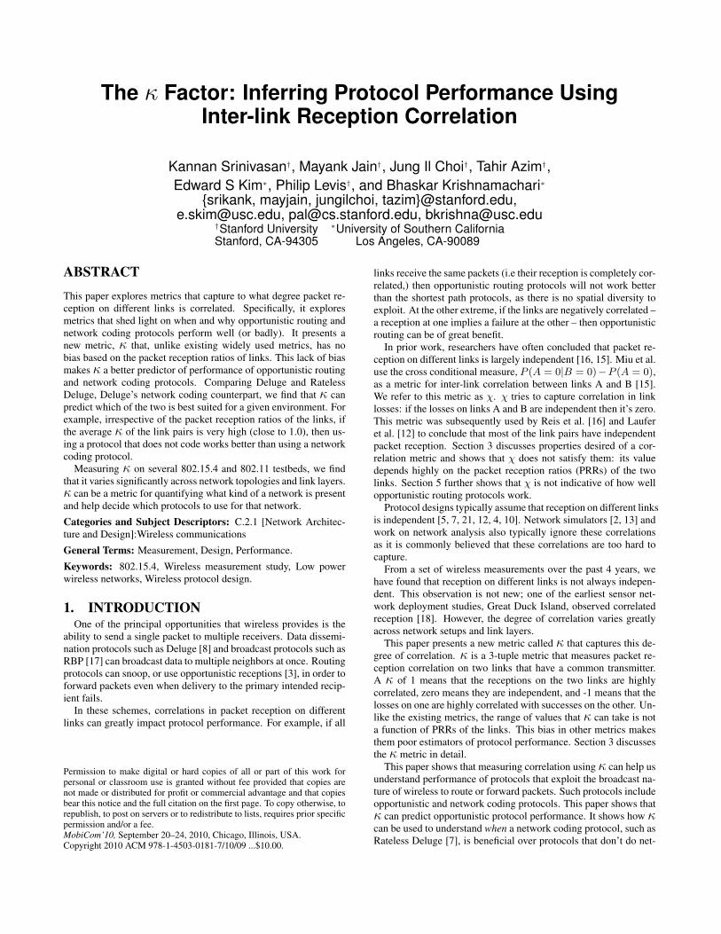
Figure 2: Reception success (white) and failure (black) patternson a link pair with perfectly positive correlation.

(a) Simplest Scenario(PRRs sum to 1.0)

(b) General Scenario(PRRs don’t sum to 1.0)

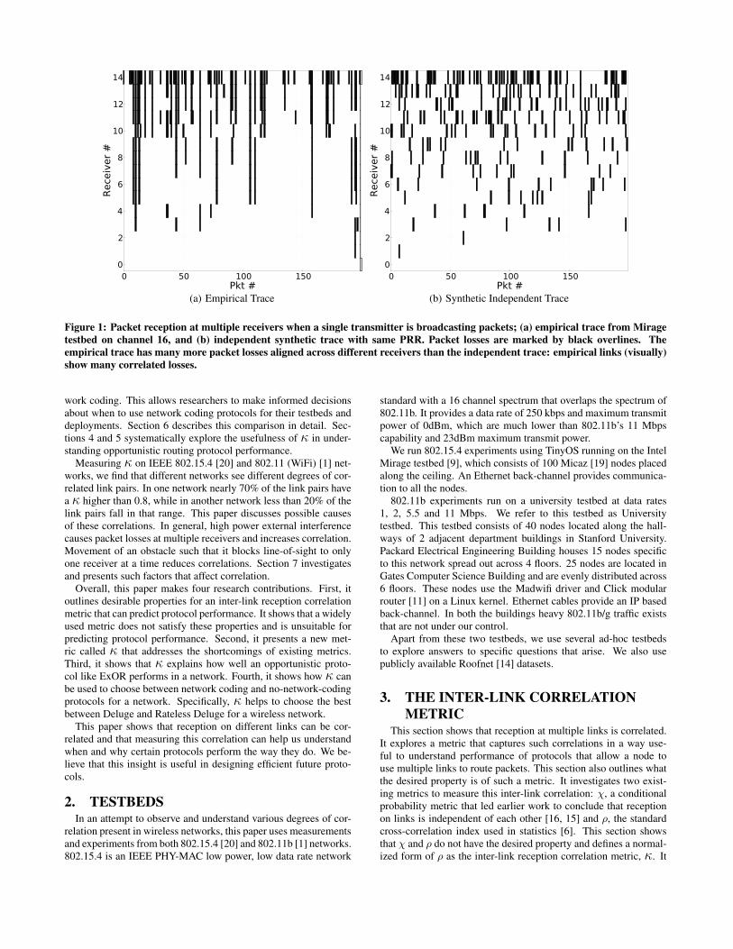
Figure 3: Reception success (white) and failure (black) scenar-ios on a link pair with perfectly negative correlation.

presentsκmeasurements for several 802.15.4 and 802.11 testbeds,showing that κ varies across networks and link layers.

3.1 Correlated LossesA small experiment shows inter-link reception correlations. A

single node on the Mirage testbed transmits 200 broadcast pack-ets on channel 16. All the nodes that hear the packets report to acentralized server.

Figure 1(a) shows packet reception at different receivers fromempirical measurements. Packet losses are marked by black over-lines. Long vertical overlines indicate that packets are lost at multi-ple receivers. For visual comparison, Figure 1(b) shows how recep-tion across receivers looks like when losses are independent usingsynthetically generated traces. The comparison shows that packetlosses on different links in Figure 1(a), from empirical measure-ments, are correlated. While Figure 1 shows that reception correla-tions exist, quantifying such correlations is desirable in understand-ing their implications to protocol performance.

3.2 Desired PropertyOne of the goals of this work is to explore a metric that captures

inter-link reception correlation in a way meaningful to understandprotocols that use multiple links simultaneously to route packets.Examples of such protocols include opportunistic routing and net-work coding protocols. In such protocols, every node chooses a setof links, from all the available links, to reduce number of transmis-sions to let a packet make progress towards destination.

After choosing the first link, a node has to carefully choose thenext link in the set. The node does not improve the chances of apacket making progress if transmissions that succeed on the sec-ond link are a subset of transmissions that succeed on the first link.It’s desirable for our metric to identify such link pairs as perfectlypositively correlated. Figures 2(a) and 2(b) show perfectly posi-tively correlated link pairs for two different cases; when both thelinks have same PRR and when they have different PRRs.

On the other hand, if the second link’s transmissions that fail area subset of transmissions that succeed on the first link, then a nodemaximizes the chances of every packet making progress. It’s desir-able for our metric to identify such link pairs as perfectly negativelycorrelated. Figures 3(a) and 3(b) show perfectly negatively corre-lated link pairs for two different cases; when the PRRs of the twolinks sum to 1 and when the PRRs don’t sum to 1.

3.3 Exploring Correlation Metric: χPrevious work has used cross-conditional probability, χ, as the

inter-link correlation metric [16, 15]. χ is a 3-tuple quantity, de-fined on a transmitter, t, and two receivers, x and y, that can hearpackets from t, as:

χt,x,y = P(t)

x/y(0/0)− P(t)x (0), (1)

where, P (t)

x/y(0/0) is the probability, when t transmits, that apacket failed on link t→x given that it failed on link t→y andP

(t)x (0) is the probability that a packet failed on link t→x. If the

failures on the two links, t→x and t→y are independent then χ is0.

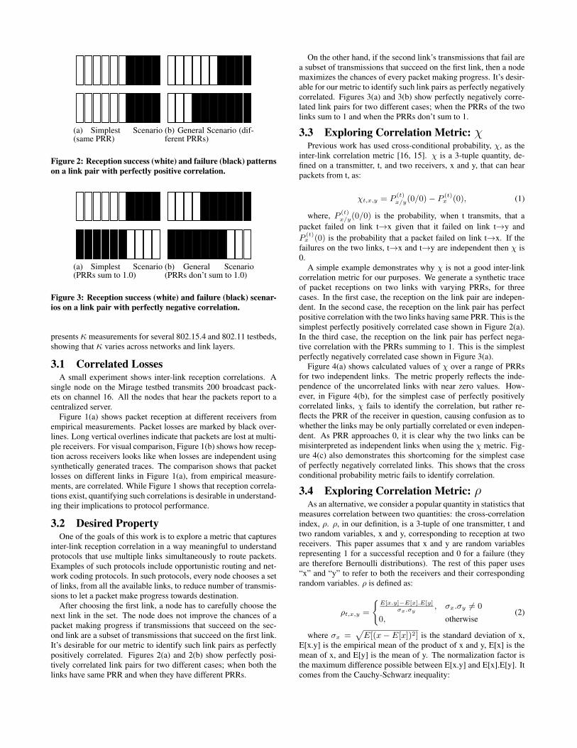
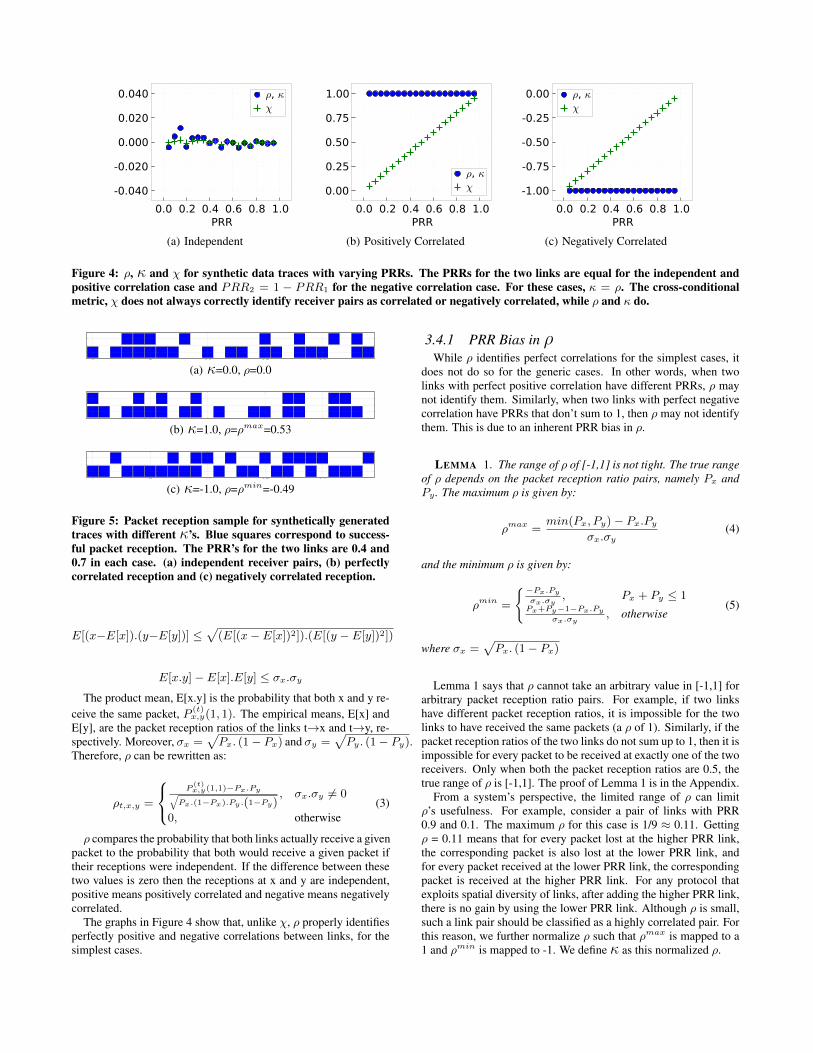
A simple example demonstrates why χ is not a good inter-linkcorrelation metric for our purposes. We generate a synthetic traceof packet receptions on two links with varying PRRs, for threecases. In the first case, the reception on the link pair are indepen-dent. In the second case, the reception on the link pair has perfectpositive correlation with the two links having same PRR. This is thesimplest perfectly positively correlated case shown in Figure 2(a).In the third case, the reception on the link pair has perfect nega-tive correlation with the PRRs summing to 1. This is the simplestperfectly negatively correlated case shown in Figure 3(a).

Figure 4(a) shows calculated values of χ over a range of PRRsfor two independent links. The metric properly reflects the inde-pendence of the uncorrelated links with near zero values. How-ever, in Figure 4(b), for the simplest case of perfectly positivelycorrelated links, χ fails to identify the correlation, but rather re-flects the PRR of the receiver in question, causing confusion as towhether the links may be only partially correlated or even indepen-dent. As PRR approaches 0, it is clear why the two links can bemisinterpreted as independent links when using the χ metric. Fig-ure 4(c) also demonstrates this shortcoming for the simplest caseof perfectly negatively correlated links. This shows that the crossconditional probability metric fails to identify correlation.

3.4 Exploring Correlation Metric: ρAs an alternative, we consider a popular quantity in statistics that

measures correlation between two quantities: the cross-correlationindex, ρ. ρ, in our definition, is a 3-tuple of one transmitter, t andtwo random variables, x and y, corresponding to reception at tworeceivers. This paper assumes that x and y are random variablesrepresenting 1 for a successful reception and 0 for a failure (theyare therefore Bernoulli distributions). The rest of this paper uses“x” and “y” to refer to both the receivers and their correspondingrandom variables. ρ is defined as:

ρt,x,y =

{E[x.y]−E[x].E[y]

σx.σy, σx.σy 6= 0

0, otherwise(2)

where σx =√E[(x− E[x])2] is the standard deviation of x,

E[x.y] is the empirical mean of the product of x and y, E[x] is themean of x, and E[y] is the mean of y. The normalization factor isthe maximum difference possible between E[x.y] and E[x].E[y]. Itcomes from the Cauchy-Schwarz inequality:

0.0 0.2 0.4 0.6 0.8 1.0PRR

-0.040

-0.020

0.000

0.020

0.040 ρ, κχ

(a) Independent

0.0 0.2 0.4 0.6 0.8 1.0PRR

0.00

0.25

0.50

0.75

1.00

ρ, κχ

(b) Positively Correlated

0.0 0.2 0.4 0.6 0.8 1.0PRR

-1.00

-0.75

-0.50

-0.25

0.00 ρ, κχ

(c) Negatively Correlated

Figure 4: ρ, κ and χ for synthetic data traces with varying PRRs. The PRRs for the two links are equal for the independent andpositive correlation case and PRR2 = 1 − PRR1 for the negative correlation case. For these cases, κ = ρ. The cross-conditionalmetric, χ does not always correctly identify receiver pairs as correlated or negatively correlated, while ρ and κ do.

0 5 10 15 200.5

1.0

1.5

2.0

2.5

(a) κ=0.0, ρ=0.0

0 5 10 15 200.5

1.0

1.5

2.0

2.5

(b) κ=1.0, ρ=ρmax=0.53

0 5 10 15 200.5

1.0

1.5

2.0

2.5

(c) κ=-1.0, ρ=ρmin=-0.49

Figure 5: Packet reception sample for synthetically generatedtraces with different κ’s. Blue squares correspond to success-ful packet reception. The PRR’s for the two links are 0.4 and0.7 in each case. (a) independent receiver pairs, (b) perfectlycorrelated reception and (c) negatively correlated reception.

E[(x−E[x]).(y−E[y])] ≤√

(E[(x− E[x])2]).(E[(y − E[y])2])

E[x.y]− E[x].E[y] ≤ σx.σyThe product mean, E[x.y] is the probability that both x and y re-

ceive the same packet, P (t)x,y(1, 1). The empirical means, E[x] and

E[y], are the packet reception ratios of the links t→x and t→y, re-spectively. Moreover, σx =

√Px. (1− Px) and σy =

√Py. (1− Py).

Therefore, ρ can be rewritten as:

ρt,x,y =

P

(t)x,y(1,1)−Px.Py√

Px.(1−Px).Py.(1−Py), σx.σy 6= 0

0, otherwise(3)

ρ compares the probability that both links actually receive a givenpacket to the probability that both would receive a given packet iftheir receptions were independent. If the difference between thesetwo values is zero then the receptions at x and y are independent,positive means positively correlated and negative means negativelycorrelated.

The graphs in Figure 4 show that, unlike χ, ρ properly identifiesperfectly positive and negative correlations between links, for thesimplest cases.

3.4.1 PRR Bias in ρWhile ρ identifies perfect correlations for the simplest cases, it

does not do so for the generic cases. In other words, when twolinks with perfect positive correlation have different PRRs, ρ maynot identify them. Similarly, when two links with perfect negativecorrelation have PRRs that don’t sum to 1, then ρ may not identifythem. This is due to an inherent PRR bias in ρ.

LEMMA 1. The range of ρ of [-1,1] is not tight. The true rangeof ρ depends on the packet reception ratio pairs, namely Px andPy . The maximum ρ is given by:

ρmax =min(Px, Py)− Px.Py

σx.σy(4)

and the minimum ρ is given by:

ρmin =

{−Px.Py

σx.σy, Px + Py ≤ 1

Px+Py−1−Px.Py

σx.σy, otherwise

(5)

where σx =√Px. (1− Px)

Lemma 1 says that ρ cannot take an arbitrary value in [-1,1] forarbitrary packet reception ratio pairs. For example, if two linkshave different packet reception ratios, it is impossible for the twolinks to have received the same packets (a ρ of 1). Similarly, if thepacket reception ratios of the two links do not sum up to 1, then it isimpossible for every packet to be received at exactly one of the tworeceivers. Only when both the packet reception ratios are 0.5, thetrue range of ρ is [-1,1]. The proof of Lemma 1 is in the Appendix.

From a system’s perspective, the limited range of ρ can limitρ’s usefulness. For example, consider a pair of links with PRR0.9 and 0.1. The maximum ρ for this case is 1/9 ≈ 0.11. Gettingρ = 0.11 means that for every packet lost at the higher PRR link,the corresponding packet is also lost at the lower PRR link, andfor every packet received at the lower PRR link, the correspondingpacket is received at the higher PRR link. For any protocol thatexploits spatial diversity of links, after adding the higher PRR link,there is no gain by using the lower PRR link. Although ρ is small,such a link pair should be classified as a highly correlated pair. Forthis reason, we further normalize ρ such that ρmax is mapped to a1 and ρmin is mapped to -1. We define κ as this normalized ρ.

(a) Channel 26, Power 0dBm (b) Channel 26, Power -25dBm

(c) Channel 16, Power 0dBm (d) Channel 16, Power -25dBm

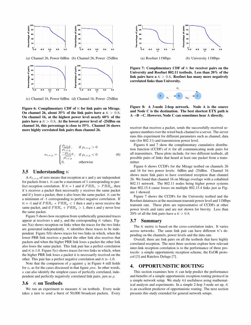
Figure 6: Complimentary CDF of κ for link pairs on Mirage.On channel 26, about 35% of the link pairs have a κ > 0.8.On channel 16, at the highest power level nearly 60% of thepairs have a κ > 0.8. At the lowest power level of -25dBm onchannel 16, this percentage is close to 55%. Channel 16 showsmore highly correlated link pairs than channel 26.

κt,x,y =

ρt,x,yρmaxt,x,y

, if ρt,x,y > 0

−ρt,x,yρmint,x,y

, if ρt,x,y < 0

0, otherwise

(6)

3.5 Understanding κA κt,x,y of zero means that reception at x and y are independent

for packets from t. κ can be a maximum of 1 corresponding to per-fect reception correlation. If κ = 1 and if PRRx > PRRy , thenif x receives a packet then necessarily y receives the same packetand if y loses a packet, then x also loses the same packet. κ can bea minimum of -1 corresponding to perfect negative correlation. Ifκ = -1 and if PRRx + PRRy < 1 then x and y never receive thesame packet, and if PRRx + PRRy > 1, then x and y never losethe same packet.

Figure 5 shows how reception from synthetically generated tracesappear at receivers x and y, and the corresponding κ values. Fig-ure 5(a) shows reception on links when the traces for the two linksare generated independently. κ identifies these traces to be inde-pendent. Figure 5(b) shows traces for two links in which, when thelower PRR link receives a packet the other link also receives thatpackets and when the higher PRR link loses a packet the other linkalso loses the same packet. This link pair has a perfect correlationand κ is 1.0. Figure 5(c) shows traces for two links in which, whenthe higher PRR link loses a packet it is necessarily received on theother. This pair has a perfect negative correlation and κ is -1.0.

Note that the comparison of ρ against χ in Figure 4 still holdsfor κ, as for the cases discussed in that figure ρ=κ. In other words,κ can also identify the simplest cases of perfectly correlated, inde-pendent and perfectly negatively correlated link pairs, just as ρ.

3.6 κ on TestbedsWe run an experiment to measure κ on testbeds. Every node

takes a turn to send a burst of 50,000 broadcast packets. Every

(a) Roofnet 11Mbps (b) University 11Mbps

Figure 7: Complimentary CDF of κ for receiver pairs on theUniversity and Roofnet 802.11 testbeds. Less than 20% of thelink pairs have a κ > 0.8. Roofnet has many more negativelycorrelated links than University.

A B CPx PBC

Py

Figure 8: A 3-node 2-hop network. Node A is the sourceand Node C is the destination. The best shortest ETX path isA→B→C. However, Node C can sometimes hear A directly.

receiver that receives a packet, sends the successfully received se-quence numbers over the wired back-channel to a server. The serverruns this experiment for different parameters such as channel, datarate (for 802.11) and transmission power level.

Figures 6 and 7 show the complimentary cumulative distribu-tion function (CCDF) of κ for all communicating node pairs forall transmitters. These plots include, for two different testbeds, allpossible pairs of links that heard at least one packet from a trans-mitter.

Figure 6 shows CCDFs for the Mirage testbed on channels 26and 16 for two power levels: 0dBm and -25dBm. Channel 16shows more link pairs to have correlated reception than channel26. We found that channel 16 on Mirage overlaps with a cohabited802.11 network. The 802.11 nodes being higher power systemsthan 802.15.4 cause losses on multiple 802.15.4 links just as Fig-ure 1 showed.

Figure 7 shows the CCDFs for the University testbed and theRoofnet datatraces at the maximum transmit power level and 11Mbpstransmit rate. These plots are representative of CCDFs at otherpower levels and rates and are not shown for brevity. Less than20% of all the link pairs have a κ > 0.8.

3.7 SummaryThe κ metric is based on the cross-correlation index. It varies

across networks. The same link pair can have different κ’s de-pending on the channels, power levels and the data rate.

Overall, there are link pairs on all the testbeds that have highlycorrelated reception. The next three sections explore how relevantinter-link reception correlation is to the performance of three pro-tocols: a simple opportunistic reception scheme, the ExOR proto-col [3] and Rateless Deluge [7].

4. OPPORTUNISTIC ROUTINGThis section examines how κ can help predict the performance

and benefits of a simple opportunistic reception routing protocol ina simple network setup. We study κs usefulness using mathemat-ical analysis and experiments. In a simple 2-hop 3-node set up, κis an excellent predictor of opportunistic routing. The next sectionpresents this study extended for general network setups.

-1.0 -0.5 0.0 0.5 1.00

2

4

6

8

10

An

yp

ath

ETX

PBC = 1.0PBC = 0.2

(a) Anypath ETX

-1.0 -0.5 0.0 0.5 1.0-1.0

-0.5

0.0

0.5

1.0

An

yp

ath

ETX

Rati

o PBC = 1.0PBC = 0.2

(b) Anypath ETX Ratio

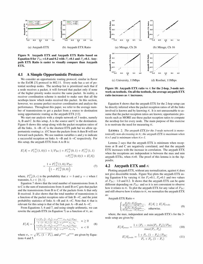
Figure 9: Anypath ETX and Anypath ETX Ratio based onEquation 8 for PBC=1.0 and 0.2 with Px=0.1 and Py=0.1. Any-path ETX Ratio is easier to visually compare than AnypathETX.

4.1 A Simple Opportunistic ProtocolWe consider an opportunistic routing protocol, similar in flavor

to the ExOR [3] protocol in 802.11. Every node has a set of po-tential nexthop nodes. The nexthop list is prioritized such that ifa node receives a packet, it will forward that packet only if noneof the higher priority nodes receive the same packet. In reality, areceiver coordination scheme is needed to make sure that all thenexthops know which nodes received this packet. In this section,however, we assume perfect receiver coordination and analyze theperformance. Throughout this paper, we refer to the average num-ber of transmissions to get a packet from a source to destinationusing opportunistic routing as the anypath ETX [12].

We start our analysis with a simple network of 3 nodes, namelyA, B and C. In this setup, A is the source and C is the destination.Figure 8 shows this setup along with the packet reception ratios ofall the links. A→B→C is the shortest ETX path but we allow op-portunistic routing i.e. if C hears the packets from A then B will notforward such packets. We use random variables x and y to indicatea successful reception on links A→B and A→C respectively. Forthis setup, the anypath ETX from A to B is:

E[A] = P (A)x,y (1, 0)(1 + 1/PBC) + P (A)

x,y (0, 1) + P (A)x,y (1, 1)

+P (A)x,y (0, 0)(1 + E[A])

=1 + P

(A)x,y (1, 0)/PBC(

1− P (A)x,y (0, 0)

) (7)

where, P (t)x,y(b, c) is the probability that x = b and y = c when t

transmits, b, c ∈ {0, 1}.Equation 7 shows that the total number of transmissions from A

to C is the sum of transmissions from A until B or C gets that packetand the transmissions from B to C of the packets from A that onlyB received. It also shows that the total number of transmissions isa function of the packet reception ratio of link B→C, and the jointprobability statistics of links A→B and A→C. Note that κ that isrelevant for this setup is that of the link pair A→B and A→C.

From Equations 3, 6 and 7, and using simple arithmetic, we canrewrite the anypath ETX (in Equation 7) as a function of κ, as:

E[A] =

1+[Px.(1−Py)−κ.ρmax.σx.σy ]/PBC

1−(1−Px).(1−Py)−κ.ρmax.σx.σy, κ ≥ 0

1+[Px.(1−Py)−κ.ρmin.σx.σy ]/PBC

1−(1−Px).(1−Py)−κ.ρmin.σx.σy, κ < 0

(8)

where σx =√Px. (1− Px), and ρmax, ρmin are given by Equa-

tions 4 and 5.

(a) Mirage, Ch 26 (b) Mirage, Ch 16

(c) University, 11Mbps (d) Roofnet, 11Mbps

Figure 10: Anypath ETX ratio vs κ for the 2-hop, 3-node net-work on testbeds. On all the testbeds, the average anypath ETXratio increases as κ increases.

Equation 8 shows that the anypath ETX for the 2-hop setup canbe directly inferred when the packet reception ratios of all the linksinvolved is known and by knowing κ. It is not unreasonable to as-sume that the packet reception ratios are known; opportunistic pro-tocols such as MORE use these packet reception ratios to computethe nexthop list for every node. The main purpose of this exerciseis to motivate the need for measuring κ.

LEMMA 2. The anypath ETX for the 3-node network is mono-tonically non-decreasing in κ; the anypath ETX is maximum whenκ=1 and is minimum when κ=-1.

Lemma 2 says that the anypath ETX is minimum when recep-tions at B and C are negatively correlated, and that the anypathETX increases with the increase in correlation. The anypath ETXwhen the receptions are independent is between the max and minanypath ETXs, when κ=0. The proof of this lemma is in the Ap-pendix.

4.2 Anypath ETX and κPlotting anypath ETX, without any normalization, againstκ does

not give discernible trends. Figure 9(a) plots the anypath ETX us-ing Equation 8 by varying κ for Px=0.1, Py=0.1 and two valuesof PBC : 1.0 and 0.2. It shows that the anypath ETX can be quitedifferent depending on PBC and so it is not convenient to observehow it relates to κ. To plot the anypath ETX for any value of PBCand still observe how it relates toκ, we normalize the anypath ETXas:

Anypath ETX Ratio ={E[A]−E[A]inde

E[A]max−E[A]inde, E[A] ≥ E[A]inde

E[A]−E[A]indeE[A]inde−E[A]min

, otherwise.(9)

where, the max, independent and min anypath ETX’s for the 3-node setup are given by:

E[A]max =1 + (Px −min(Px, Py))/PBC

max(Px, Py)(10)

E[A]inde =1 + Px. (1− Py) /PBCPx + Py. (1− Px)

(11)

E[A]min =

{1+Px/PBCPx+Py

, Px + Py ≤ 1

1 + (1− Py) /PBC , otherwise.(12)

The anypath ETX ratio is zero when the true anypath ETX matchesthe anypath ETX computed by assuming inter-link receptions to beindependent. Note that the opportunistic routing protocols makethis independent assumption and so an anypath ETX ratio of zeromeans that the estimate from the opportunistic routing protocolsmatch the true anypath ETX. The ratio is positive when opportunis-tic routing protocol under-estimates the anypath ETX, with a maxi-mum of 1 when the under-estimation is the maximum. The anypathETX ratio is negative when the ETX is over-estimated, with a min-imum of -1 when the over-estimation is the maximum.

Figure 9(b) plots the anypath ETX ratio against κ for the samesetup as in Figure 9(a). The anypath ETX ratio allows for directcomparison of paths with different PBC ’s. The anypath ETX in-creases as κ increases. This is in agreement with Lemma 2.

To validate that the monotonicity argument carries over to em-pirical results, we analyze the anypath ETX for the same Mirage,University and Roofnet datatraces as in Section 3.6. We look atall the cases where a node, A can send packets to node C, eitherdirectly or through B. For all such cases, we compute the actualanypath ETX from A to C, using the datatraces. From this anypathETX, we compute the anypath ETX ratio and compare it with κ ofthe link pair A→B and A→C.

Figure 10 plots the anypath ETX ratio against κ for both the802.15.4 and 802.11 testbeds. In all the testbeds, the average any-path ETX ratio increases as κ increases, as Lemma 2 pointed out.

4.3 SummaryThis section shows that κ directly correlates with the perfor-

mance of opportunistic routing in a simple 2-hop, 3-node setup.In fact, it shows that as κ increases the anypath ETX for a givensource-destination pair also monotonically increases.

5. EXTREMELY OPPORTUNISTICROUTING (EXOR)

The results presented in Section 4 are for the 3-node setup. Thissection explores if κ is useful in understanding how an opportunis-tic routing protocol will perform in a general multi-hop, multiple-receiver setting.

We extend the anypath ETX computation for the general casein which node t is the source, n is the destination and the anypathtraverses through nodes 1,.., n-1.

E[t] =1

1− P (t)1,2..n(0, .., 0)

[1 + P

(t)1,2..n(1, 0, .., 0).E[1]

+P(t)2,3..n(1, 0, .., 0).E[2] + ..+ P

(t)n−1,n(1, 0).E[n− 1]

+P (t)n (1).E[n]

] (13)

5.1 Experimental MethodologyWe use the same Mirage, University and Roofnet data traces as in

Section 3.6. For every source destination pair, the source computesthe nexthop list from all the nodes that have a lower shortest pathcost to the destination than the source. It includes a node in thenexthop list if that node can send at least 10% of the packets in abatch of size 100 packets. This methodology is same as the one forExOR proposed by Biswas et al. [3].

For every node in the nexthop list, we compute the anypath ETXratio using Equation 13. For every such node, n, we compute the

(a) Mirage, Ch 26 (b) Mirage, Ch 16

(c) University, 11Mbps (d) Roofnet, 11Mbps

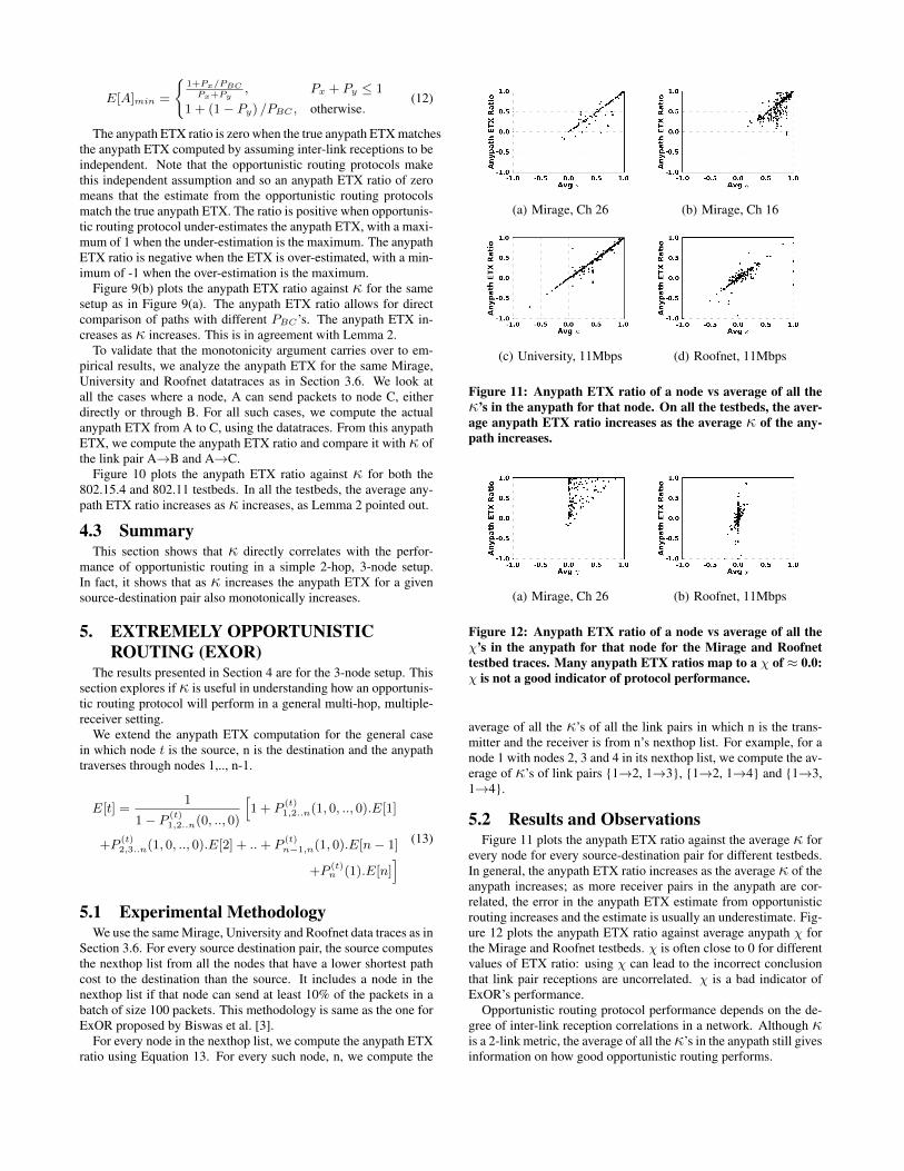
Figure 11: Anypath ETX ratio of a node vs average of all theκ’s in the anypath for that node. On all the testbeds, the aver-age anypath ETX ratio increases as the average κ of the any-path increases.

(a) Mirage, Ch 26 (b) Roofnet, 11Mbps

Figure 12: Anypath ETX ratio of a node vs average of all theχ’s in the anypath for that node for the Mirage and Roofnettestbed traces. Many anypath ETX ratios map to a χ of ≈ 0.0:χ is not a good indicator of protocol performance.

average of all the κ’s of all the link pairs in which n is the trans-mitter and the receiver is from n’s nexthop list. For example, for anode 1 with nodes 2, 3 and 4 in its nexthop list, we compute the av-erage of κ’s of link pairs {1→2, 1→3}, {1→2, 1→4} and {1→3,1→4}.

5.2 Results and ObservationsFigure 11 plots the anypath ETX ratio against the average κ for

every node for every source-destination pair for different testbeds.In general, the anypath ETX ratio increases as the average κ of theanypath increases; as more receiver pairs in the anypath are cor-related, the error in the anypath ETX estimate from opportunisticrouting increases and the estimate is usually an underestimate. Fig-ure 12 plots the anypath ETX ratio against average anypath χ forthe Mirage and Roofnet testbeds. χ is often close to 0 for differentvalues of ETX ratio: using χ can lead to the incorrect conclusionthat link pair receptions are uncorrelated. χ is a bad indicator ofExOR’s performance.

Opportunistic routing protocol performance depends on the de-gree of inter-link reception correlations in a network. Although κis a 2-link metric, the average of all theκ’s in the anypath still givesinformation on how good opportunistic routing performs.

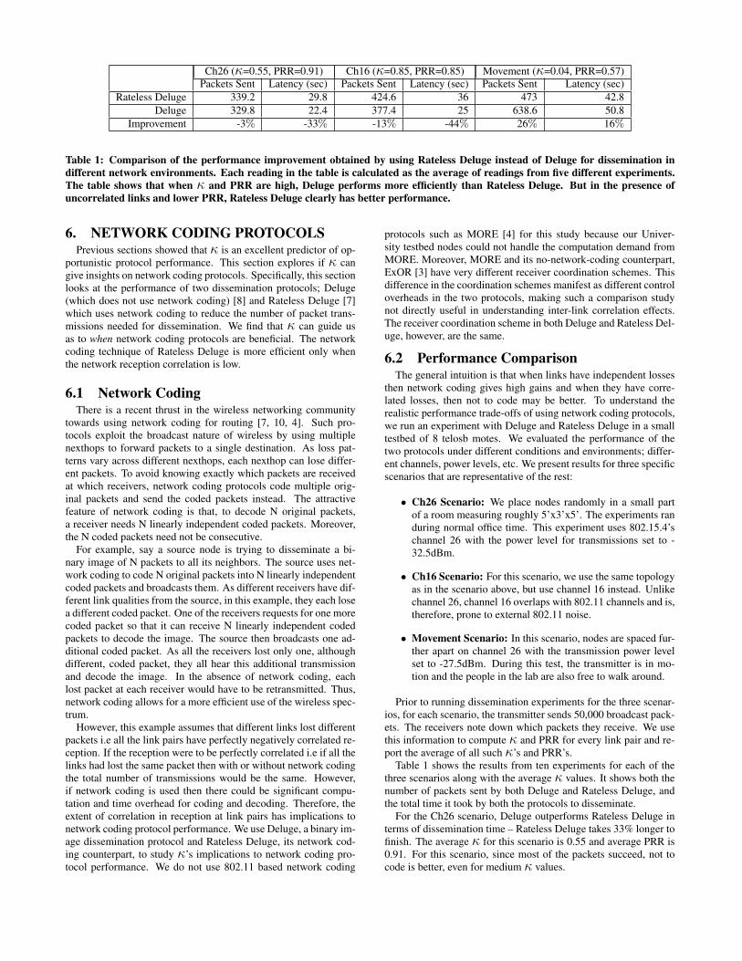
Ch26 (κ=0.55, PRR=0.91) Ch16 (κ=0.85, PRR=0.85) Movement (κ=0.04, PRR=0.57)Packets Sent Latency (sec) Packets Sent Latency (sec) Packets Sent Latency (sec)

Rateless Deluge 339.2 29.8 424.6 36 473 42.8Deluge 329.8 22.4 377.4 25 638.6 50.8

Improvement -3% -33% -13% -44% 26% 16%

Table 1: Comparison of the performance improvement obtained by using Rateless Deluge instead of Deluge for dissemination indifferent network environments. Each reading in the table is calculated as the average of readings from five different experiments.The table shows that when κ and PRR are high, Deluge performs more efficiently than Rateless Deluge. But in the presence ofuncorrelated links and lower PRR, Rateless Deluge clearly has better performance.

6. NETWORK CODING PROTOCOLSPrevious sections showed that κ is an excellent predictor of op-

portunistic protocol performance. This section explores if κ cangive insights on network coding protocols. Specifically, this sectionlooks at the performance of two dissemination protocols; Deluge(which does not use network coding) [8] and Rateless Deluge [7]which uses network coding to reduce the number of packet trans-missions needed for dissemination. We find that κ can guide usas to when network coding protocols are beneficial. The networkcoding technique of Rateless Deluge is more efficient only whenthe network reception correlation is low.

6.1 Network CodingThere is a recent thrust in the wireless networking community

towards using network coding for routing [7, 10, 4]. Such pro-tocols exploit the broadcast nature of wireless by using multiplenexthops to forward packets to a single destination. As loss pat-terns vary across different nexthops, each nexthop can lose differ-ent packets. To avoid knowing exactly which packets are receivedat which receivers, network coding protocols code multiple orig-inal packets and send the coded packets instead. The attractivefeature of network coding is that, to decode N original packets,a receiver needs N linearly independent coded packets. Moreover,the N coded packets need not be consecutive.

For example, say a source node is trying to disseminate a bi-nary image of N packets to all its neighbors. The source uses net-work coding to code N original packets into N linearly independentcoded packets and broadcasts them. As different receivers have dif-ferent link qualities from the source, in this example, they each losea different coded packet. One of the receivers requests for one morecoded packet so that it can receive N linearly independent codedpackets to decode the image. The source then broadcasts one ad-ditional coded packet. As all the receivers lost only one, althoughdifferent, coded packet, they all hear this additional transmissionand decode the image. In the absence of network coding, eachlost packet at each receiver would have to be retransmitted. Thus,network coding allows for a more efficient use of the wireless spec-trum.

However, this example assumes that different links lost differentpackets i.e all the link pairs have perfectly negatively correlated re-ception. If the reception were to be perfectly correlated i.e if all thelinks had lost the same packet then with or without network codingthe total number of transmissions would be the same. However,if network coding is used then there could be significant compu-tation and time overhead for coding and decoding. Therefore, theextent of correlation in reception at link pairs has implications tonetwork coding protocol performance. We use Deluge, a binary im-age dissemination protocol and Rateless Deluge, its network cod-ing counterpart, to study κ’s implications to network coding pro-tocol performance. We do not use 802.11 based network coding

protocols such as MORE [4] for this study because our Univer-sity testbed nodes could not handle the computation demand fromMORE. Moreover, MORE and its no-network-coding counterpart,ExOR [3] have very different receiver coordination schemes. Thisdifference in the coordination schemes manifest as different controloverheads in the two protocols, making such a comparison studynot directly useful in understanding inter-link correlation effects.The receiver coordination scheme in both Deluge and Rateless Del-uge, however, are the same.

6.2 Performance ComparisonThe general intuition is that when links have independent losses

then network coding gives high gains and when they have corre-lated losses, then not to code may be better. To understand therealistic performance trade-offs of using network coding protocols,we run an experiment with Deluge and Rateless Deluge in a smalltestbed of 8 telosb motes. We evaluated the performance of thetwo protocols under different conditions and environments; differ-ent channels, power levels, etc. We present results for three specificscenarios that are representative of the rest:

• Ch26 Scenario: We place nodes randomly in a small partof a room measuring roughly 5’x3’x5’. The experiments randuring normal office time. This experiment uses 802.15.4’schannel 26 with the power level for transmissions set to -32.5dBm.

• Ch16 Scenario: For this scenario, we use the same topologyas in the scenario above, but use channel 16 instead. Unlikechannel 26, channel 16 overlaps with 802.11 channels and is,therefore, prone to external 802.11 noise.

• Movement Scenario: In this scenario, nodes are spaced fur-ther apart on channel 26 with the transmission power levelset to -27.5dBm. During this test, the transmitter is in mo-tion and the people in the lab are also free to walk around.

Prior to running dissemination experiments for the three scenar-ios, for each scenario, the transmitter sends 50,000 broadcast pack-ets. The receivers note down which packets they receive. We usethis information to compute κ and PRR for every link pair and re-port the average of all such κ’s and PRR’s.

Table 1 shows the results from ten experiments for each of thethree scenarios along with the average κ values. It shows both thenumber of packets sent by both Deluge and Rateless Deluge, andthe total time it took by both the protocols to disseminate.

For the Ch26 scenario, Deluge outperforms Rateless Deluge interms of dissemination time – Rateless Deluge takes 33% longer tofinish. The average κ for this scenario is 0.55 and average PRR is0.91. For this scenario, since most of the packets succeed, not tocode is better, even for medium κ values.

0 0.2 0.4 0.6 0.8 1.0κ

0

20

40

60

80

100

Tim

e (

seco

nds)

Deluge

Rateless Deluge

(a) PRR = 0.4

0 0.2 0.4 0.6 0.8 1.0κ

0

20

40

60

80

100

Tim

e (

seco

nds)

Deluge

Rateless Deluge

(b) PRR = 0.6

0 0.2 0.4 0.6 0.8 1.0κ

0

20

40

60

80

100

Tim

e (

seco

nds)

Deluge

Rateless Deluge

(c) PRR = 0.8

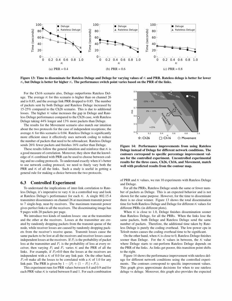
Figure 13: Time to disseminate for Rateless Deluge and Deluge for varying values of κ and PRR. Rateless deluge is better for lowerκ, but Deluge is better for higher κ. The performance switch point varies based on the PRR of the links.

For the Ch16 scenario also, Deluge outperforms Rateless Del-uge. The average κ for this scenario is higher than on channel 26and is 0.85, and the average link PRR dropped to 0.85. The numberof packets sent by both Deluge and Rateless Deluge increased by15-25% compared to the Ch26 scenario. This is due to additionallosses. The higher κ value increases the gap in Deluge and Rate-less Deluge performance compared to the Ch26 case, with RatelessDeluge taking 44% longer and 13% more packets than Deluge.

The results for the Movement scenario also match our intuitionabout the two protocols for the case of independent receptions; theaverage κ for this scenario is 0.04. Rateless Deluge is significantlymore efficient since it effectively uses network coding to reducethe number of packets that need to be rebroadcast. Rateless Delugesends 26% fewer packets and finishes 16% earlier than Deluge.

These results follow the general intuition and reinforce that κ isa good measure of correlation. Moreover, they show that the knowl-edge of κ combined with PRR can be used to choose between cod-ing and no coding protocols. To understand exactly when it’s betterto use network coding protocol, we need to finely vary both thePRR and κ of all the links. Such a study is useful in getting ageneral rule for making a choice between the two protocols.

6.3 Controlled ExperimentTo understand the implications of inter-link correlation to Rate-

less Deluge, it’s imperative to vary κ in a controlled way and lookat Rateless Deluge’s performance for each κ. A single 802.15.4transmitter disseminates on channel 26 at maximum transmit powerto 7 single-hop, near-by receivers. The maximum transmit powergives perfect links to all the receivers. The disseminating image has9 pages with 20 packets per page.

We introduce two kinds of random losses: one at the transmitterand the other at the receivers. Losses at the transmitter are cre-ated by randomly dropping packets from the transmit queue of thenode, while receiver losses are caused by randomly dropping pack-ets from the receiver’s receive queue. Transmit losses cause thesame packets to be lost at all the receivers and receiver losses causeindependent losses at the receivers. IfPt is the probability of packetloss at the transmitter and Pr is the probability of loss at every re-ceiver, then varying Pt and Pr varies κ and the PRR of all thelinks. For example, if Pt=0.0 then the losses at the receivers areindependent with a κ of 0.0 for any link pair. On the other hand,Pr=0 make all the losses to be correlated with a κ of 1.0 for anylink pair. The PRR is given by 1− (Pt + (1− Pt) ∗ Pr).

This experiment runs for PRR values between 0.4 and 0.9 and foreach PRR valueκ is varied between 0 and 1. For each combination

Deluge is betterRateless D

eluge

is better

: Movement: Ch16: Ch26

Figure 14: Performance improvements from using RatelessDeluge instead of Deluge for different network conditions. Thecontours correspond to specific percentage improvement val-ues for the controlled experiment. Uncontrolled experimentalresults for the three cases, Ch26, Ch16, and Movement, matchwell with predicted results from the contour map.

of PRR and κ values, we run 10 experiments with Rateless Delugeand Deluge.

For all the PRRs, Rateless Deluge sends the same or fewer num-ber of packets as Deluge. This is an expected behavior and is notshown for the same purpose. However, for the time to disseminatethere is no clear winner. Figure 13 shows the total disseminationtime for both Rateless Deluge and Deluge for differentκ values fordifferent PRRs (in different plots).

When κ is close to 1.0, Deluge finishes dissemination soonerthan Rateless Deluge, for all the PRRs. When the links lose thesame packets, both Deluge and Rateless Deluge send the samenumber of packets. Therefore, the additional time taken by Rate-less Deluge is purely the coding overhead. The low-power cpu inTelosb motes causes the coding overhead time to be significant.

On the other hand, whenκ is close to 0, Rateless Deluge finishessooner than Deluge. For the κ values in between, the κ valuewhere Deluge starts to out-perform Rateless Deluge depends onthe PRR of the links. As links get poorer, this transition point shiftsto the right.

Figure 14 shows the performance improvement with rateless del-uge for different network conditions using the controlled experi-ments. The contours correspond to specific improvement values.This graph gives approximate decisions for when to use ratelessdeluge vs deluge. Moreover, this graph also provides the expected

XX

(a) Signal Variation, PositiveCorrelation

X

XInterferer

(b) Noise Variation, Positive Cor-relation

X

(c) Signal Variation, NegativeCorrelation

X

InterfererInterfererCSMA

(d) Noise Variation, NegativeCorrelation

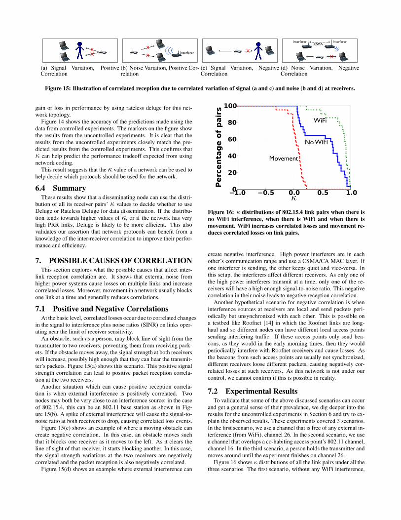
Figure 15: Illustration of correlated reception due to correlated variation of signal (a and c) and noise (b and d) at receivers.

gain or loss in performance by using rateless deluge for this net-work topology.

Figure 14 shows the accuracy of the predictions made using thedata from controlled experiments. The markers on the figure showthe results from the uncontrolled experiments. It is clear that theresults from the uncontrolled experiments closely match the pre-dicted results from the controlled experiments. This confirms thatκ can help predict the performance tradeoff expected from usingnetwork coding.

This result suggests that the κ value of a network can be used tohelp decide which protocols should be used for the network.

6.4 SummaryThese results show that a disseminating node can use the distri-

bution of all its receiver pairs’ κ values to decide whether to useDeluge or Rateless Deluge for data dissemination. If the distribu-tion tends towards higher values of κ, or if the network has veryhigh PRR links, Deluge is likely to be more efficient. This alsovalidates our assertion that network protocols can benefit from aknowledge of the inter-receiver correlation to improve their perfor-mance and efficiency.

7. POSSIBLE CAUSES OF CORRELATIONThis section explores what the possible causes that affect inter-

link reception correlation are. It shows that external noise fromhigher power systems cause losses on multiple links and increasecorrelated losses. Moreover, movement in a network usually blocksone link at a time and generally reduces correlations.

7.1 Positive and Negative CorrelationsAt the basic level, correlated losses occur due to correlated changes

in the signal to interference plus noise ratios (SINR) on links oper-ating near the limit of receiver sensitivity.

An obstacle, such as a person, may block line of sight from thetransmitter to two receivers, preventing them from receiving pack-ets. If the obstacle moves away, the signal strength at both receiverswill increase, possibly high enough that they can hear the transmit-ter’s packets. Figure 15(a) shows this scenario. This positive signalstrength correlation can lead to positive packet reception correla-tion at the two receivers.

Another situation which can cause positive reception correla-tion is when external interference is positively correlated. Twonodes may both be very close to an interference source: in the caseof 802.15.4, this can be an 802.11 base station as shown in Fig-ure 15(b). A spike of external interference will cause the signal-to-noise ratio at both receivers to drop, causing correlated loss events.

Figure 15(c) shows an example of where a moving obstacle cancreate negative correlation. In this case, an obstacle moves suchthat it blocks one receiver as it moves to the left. As it clears theline of sight of that receiver, it starts blocking another. In this case,the signal strength variations at the two receivers are negativelycorrelated and the packet reception is also negatively correlated.

Figure 15(d) shows an example where external interference can

WiFi

No WiFi

Movement

Figure 16: κ distributions of 802.15.4 link pairs when there isno WiFi interference, when there is WiFi and when there ismovement. WiFi increases correlated losses and movement re-duces correlated losses on link pairs.

create negative interference. High power interferers are in eachother’s communication range and use a CSMA/CA MAC layer. Ifone interferer is sending, the other keeps quiet and vice-versa. Inthis setup, the interferers affect different receivers. As only one ofthe high power interferers transmit at a time, only one of the re-ceivers will have a high enough signal-to-noise ratio. This negativecorrelation in their noise leads to negative reception correlation.

Another hypothetical scenario for negative correlation is wheninterference sources at receivers are local and send packets peri-odically but unsynchronized with each other. This is possible ona testbed like Roofnet [14] in which the Roofnet links are long-haul and so different nodes can have different local access pointssending interfering traffic. If these access points only send bea-cons, as they would in the early morning times, then they wouldperiodically interfere with Roofnet receivers and cause losses. Asthe beacons from such access points are usually not synchronized,different receivers loose different packets, causing negatively cor-related losses at such receivers. As this network is not under ourcontrol, we cannot confirm if this is possible in reality.

7.2 Experimental ResultsTo validate that some of the above discussed scenarios can occur

and get a general sense of their prevalence, we dig deeper into theresults for the uncontrolled experiments in Section 6 and try to ex-plain the observed results. These experiments covered 3 scenarios.In the first scenario, we use a channel that is free of any external in-terference (from WiFi), channel 26. In the second scenario, we usea channel that overlaps a co-habiting access point’s 802.11 channel,channel 16. In the third scenario, a person holds the transmitter andmoves around until the experiment finishes on channel 26.

Figure 16 shows κ distributions of all the link pairs under all thethree scenarios. The first scenario, without any WiFi interference,

0.0 0.5 1.0 1.5 2.0time (in secs)

100

90

80

70

60

50

Nois

e (

dB

m)

0.0 0.5 1.0 1.5 2.0time (in secs)

100

90

80

70

60

50

Nois

e (

dB

m)

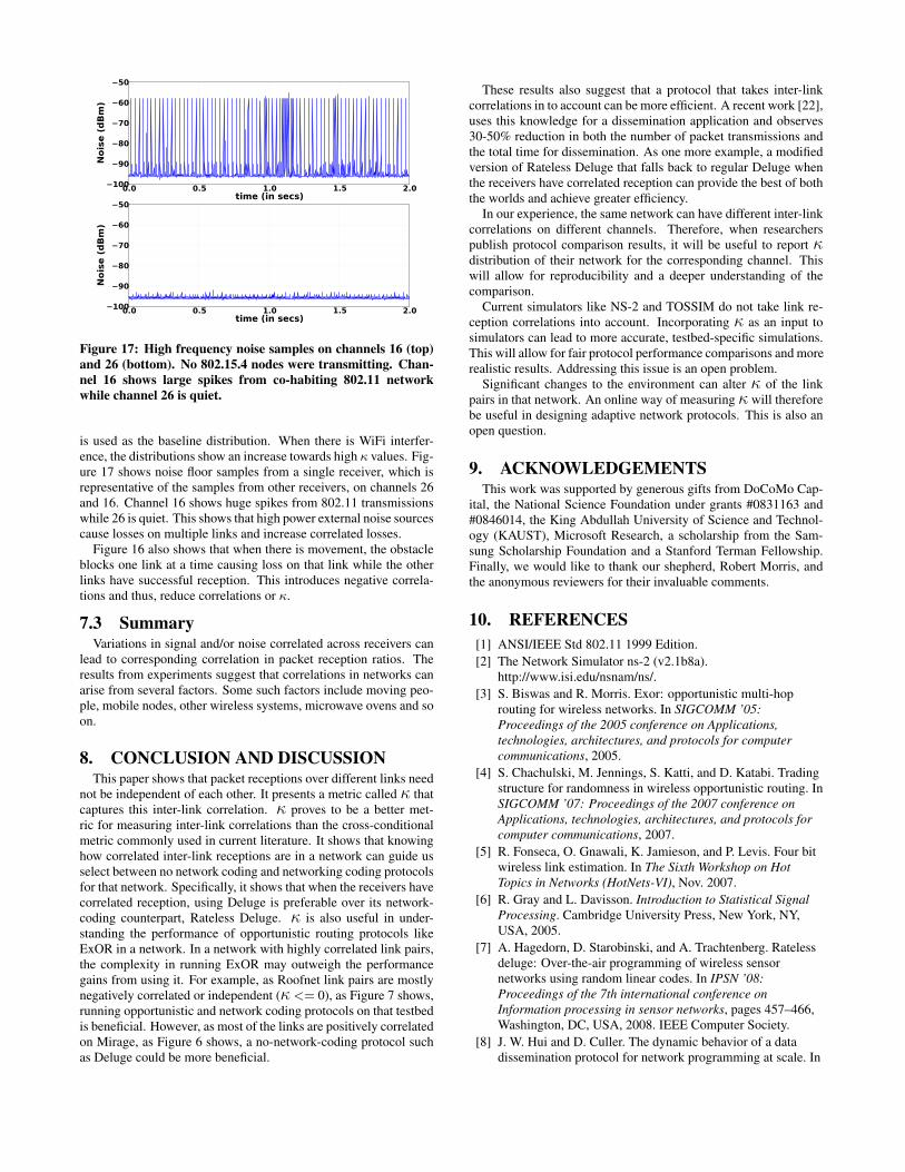
Figure 17: High frequency noise samples on channels 16 (top)and 26 (bottom). No 802.15.4 nodes were transmitting. Chan-nel 16 shows large spikes from co-habiting 802.11 networkwhile channel 26 is quiet.

is used as the baseline distribution. When there is WiFi interfer-ence, the distributions show an increase towards high κ values. Fig-ure 17 shows noise floor samples from a single receiver, which isrepresentative of the samples from other receivers, on channels 26and 16. Channel 16 shows huge spikes from 802.11 transmissionswhile 26 is quiet. This shows that high power external noise sourcescause losses on multiple links and increase correlated losses.

Figure 16 also shows that when there is movement, the obstacleblocks one link at a time causing loss on that link while the otherlinks have successful reception. This introduces negative correla-tions and thus, reduce correlations or κ.

7.3 SummaryVariations in signal and/or noise correlated across receivers can

lead to corresponding correlation in packet reception ratios. Theresults from experiments suggest that correlations in networks canarise from several factors. Some such factors include moving peo-ple, mobile nodes, other wireless systems, microwave ovens and soon.

8. CONCLUSION AND DISCUSSIONThis paper shows that packet receptions over different links need

not be independent of each other. It presents a metric called κ thatcaptures this inter-link correlation. κ proves to be a better met-ric for measuring inter-link correlations than the cross-conditionalmetric commonly used in current literature. It shows that knowinghow correlated inter-link receptions are in a network can guide usselect between no network coding and networking coding protocolsfor that network. Specifically, it shows that when the receivers havecorrelated reception, using Deluge is preferable over its network-coding counterpart, Rateless Deluge. κ is also useful in under-standing the performance of opportunistic routing protocols likeExOR in a network. In a network with highly correlated link pairs,the complexity in running ExOR may outweigh the performancegains from using it. For example, as Roofnet link pairs are mostlynegatively correlated or independent (κ <= 0), as Figure 7 shows,running opportunistic and network coding protocols on that testbedis beneficial. However, as most of the links are positively correlatedon Mirage, as Figure 6 shows, a no-network-coding protocol suchas Deluge could be more beneficial.

These results also suggest that a protocol that takes inter-linkcorrelations in to account can be more efficient. A recent work [22],uses this knowledge for a dissemination application and observes30-50% reduction in both the number of packet transmissions andthe total time for dissemination. As one more example, a modifiedversion of Rateless Deluge that falls back to regular Deluge whenthe receivers have correlated reception can provide the best of boththe worlds and achieve greater efficiency.

In our experience, the same network can have different inter-linkcorrelations on different channels. Therefore, when researcherspublish protocol comparison results, it will be useful to report κdistribution of their network for the corresponding channel. Thiswill allow for reproducibility and a deeper understanding of thecomparison.

Current simulators like NS-2 and TOSSIM do not take link re-ception correlations into account. Incorporating κ as an input tosimulators can lead to more accurate, testbed-specific simulations.This will allow for fair protocol performance comparisons and morerealistic results. Addressing this issue is an open problem.

Significant changes to the environment can alter κ of the linkpairs in that network. An online way of measuring κ will thereforebe useful in designing adaptive network protocols. This is also anopen question.

9. ACKNOWLEDGEMENTSThis work was supported by generous gifts from DoCoMo Cap-

ital, the National Science Foundation under grants #0831163 and#0846014, the King Abdullah University of Science and Technol-ogy (KAUST), Microsoft Research, a scholarship from the Sam-sung Scholarship Foundation and a Stanford Terman Fellowship.Finally, we would like to thank our shepherd, Robert Morris, andthe anonymous reviewers for their invaluable comments.

10. REFERENCES[1] ANSI/IEEE Std 802.11 1999 Edition.[2] The Network Simulator ns-2 (v2.1b8a).

http://www.isi.edu/nsnam/ns/.[3] S. Biswas and R. Morris. Exor: opportunistic multi-hop

routing for wireless networks. In SIGCOMM ’05:Proceedings of the 2005 conference on Applications,technologies, architectures, and protocols for computercommunications, 2005.

[4] S. Chachulski, M. Jennings, S. Katti, and D. Katabi. Tradingstructure for randomness in wireless opportunistic routing. InSIGCOMM ’07: Proceedings of the 2007 conference onApplications, technologies, architectures, and protocols forcomputer communications, 2007.

[5] R. Fonseca, O. Gnawali, K. Jamieson, and P. Levis. Four bitwireless link estimation. In The Sixth Workshop on HotTopics in Networks (HotNets-VI), Nov. 2007.

[6] R. Gray and L. Davisson. Introduction to Statistical SignalProcessing. Cambridge University Press, New York, NY,USA, 2005.

[7] A. Hagedorn, D. Starobinski, and A. Trachtenberg. Ratelessdeluge: Over-the-air programming of wireless sensornetworks using random linear codes. In IPSN ’08:Proceedings of the 7th international conference onInformation processing in sensor networks, pages 457–466,Washington, DC, USA, 2008. IEEE Computer Society.

[8] J. W. Hui and D. Culler. The dynamic behavior of a datadissemination protocol for network programming at scale. In

Proceedings of the Second International Conferences onEmbedded Network Sensor Systems (SenSys), 2004.

[9] Intel Research Berkeley. Mirage testbed. https://mirage.berkeley.intel-research.net/.

[10] S. Katti, H. Rahul, W. Hu, D. Katabi, M. Médard, andJ. Crowcroft. Xors in the air: practical wireless networkcoding. In SIGCOMM ’06: Proceedings of the Conferenceon Applications, technologies, architectures, and protocolsfor computer communications, 2006.

[11] E. Kohler, R. Morris, B. Chen, J. Jannotti, and M. F.Kaashoek. The Click modular router. ACM Transactions onComputer Systems, 18(3):263–297, August 2000.

[12] R. Laufer, H. Dubois-FerriÃlre, and L. Kleinrock. Multirateanypath routing in wireless mesh networks. In Proceedingsof IEEE Infocom 2009, Rio de Janeiro, Brazil, April 2009.

[13] P. Levis, N. Lee, M. Welsh, and D. Culler. TOSSIM:Simulating large wireless sensor networks of tinyos motes.In Proceedings of the First ACM Conference on EmbeddedNetworked Sensor Systems (SenSys 2003), 2003.

[14] MIT Roofnet. 802.11 testbed.http://pdos.csail.mit.edu/roofnet/.

[15] A. Miu, G. Tan, H. Balakrishnan, and J. Apostolopoulos.Divert: Fine-grained path selection for wireless lans. InProceedings of the Second International Conference onMobile Systems, Applications, and Services (MobiSys 2004),2004.

[16] C. Reis, R. Mahajan, M. Rodrig, D. Wetherall, andJ. Zahorjan. Measurement-based models of delivery andinterference in static wireless networks. In SIGCOMM, pages51–62, 2006.

[17] F. Stann, J. Heidemann, R. Shroff, and M. Z. Murtaza. RBP:Reliable broadcast propagation in wireless networks.Technical Report ISI-TR-2005-608, USC/InformationSciences Institute, November 2005.

[18] R. Szewczyk, J. Polastre, A. Mainwaring, and D. Culler.Lessons from a sensor network expedition. In Proceedings ofthe First European Workshop on Sensor Networks (EWSN),Berlin, Germany, Jan. 2004.

[19] C. Technology. Micaz datasheet. http://www.xbow.com/Products/Product_pdf_files/Wireless_pdf/MICAz_Kit_Datasheet.pdf, 2006.

[20] The Institute of Electrical and Electronics Engineers, Inc.Part 15.4: Wireless Medium Access Control (MAC) andPhysical Layer (PHY) Specifications for Low-Rate WirelessPersonal Area Networks (LR-WPANs), Oct. 2003.

[21] TinyOS. MultiHopLQI. http://www.tinyos.net/tinyos-1.x/tos/lib/MultiHopLQI, 2004.

[22] T. Zhu, Z. Zhong, T. He, and Z.-L. Zhang. Exploring linkcorrelation for efficient flooding in wireless sensor networks.In Proceedings of the First USENIX/ACM Symposium onNetwork Systems Design and Implementation (NSDI), 2010.

APPENDIXProofs of the Lemmas

Proof of Lemma 1: We wish to determine the maximum andminimum values that ρ can take on. If Px and Py are kept con-stant, then E[x] = Px, E[y] = Py, σx =

√Px · (1− Px), σy =√

Py · (1− Py) are all constant as well. From the expression of ρin Equation 2, we can see that the only variable term is E[x · y].

Thus to maximize/minimize ρ we must maximize/minimize E[x ·y].

We have that E[x · y] ≤ E[x] = Px and E[x · y] ≤ E[y] = Py .These imply that E[x · y] ≤ min (Px, Py). Assuming without lossof generality that Px ≤ Py . This inequality can be achieved as anequality by the distribution where:{Px, y(1, 1) = Px, Px,y(1, 0) = 0, Px,y(0, 1) = Py−Px, Px,y(0, 0) =

1− Py}.Thus the maximum value of E[x · y] = min (Px, Py), which

yields the maximum value of ρ indicated in Equation 4.Since (x− 1), (y− 1) are both negative, E[(x− 1) · (y− 1)] =

E[x ·y−y−x+1] ≥ 0. Rearranging terms, and noting again thatE[x] = Px, E[y] = Py , we get thatE[x·y] ≥ Px+Py−1. Further,since x and y are both non-negative random variables, we have thatE[x·y] ≥ max (0, Px + Py − 1). This inequality is achieved withequality under the following two distributions. When Px+Py ≤ 1,the following distribution minimizes E[x · y] to 0:{Px,y(1, 1) = 0, Px,y(1, 0) = Px, Px,y(0, 1) = Py, Px,y(0, 0) =

1− Px − Py}.When Px+Py ≥ 1, the following distribution minimizesE[x·y]

to Px + Py − 1:{Px,y(1, 1) = Px+Py − 1, Px,y(1, 0) = 1−Py, Px,y(0, 1) =

1− Px, Px,y(0, 0) = 0}.These minimum values of E[x · y] correspond to the minimum

values of ρ indicated in Equation 5. 2

Proof of Lemma 2: This lemma applies only if PBC > Py .This basically means that B is included as a possible next hop onlyif it has a better path to destination than A, which is a common as-sumption for opportunistic routing protocols. Under this constraint,the derivative dE[A]

dρof the expression in Equation 8 can be shown

to be:

dE[A]

dρ=

σx.σy.(PBC − Py)/PBC(1− (1− Px) . (1− Py)− ρ.σx.σy)2

(14)

where σx =√Px · (1− Px). Thus, for PBC > Py , E[A] is

monotonically non-decreasing in ρ. Further, for a given set of linkPRRs, κ ∝ ρ for both ρ > 0 and ρ < 0. Also, κ > 0 for ρ > 0,κ < 0 for ρ < 0 and κ = 0 for ρ = 0. Then, ρ is monotonicallynon-decreasing with κ. By transitivity of monotonicity, E[A] ismonotonically non-decreasing with κ. 2