


γλώσσες
Σελίδες
Νομικός

Getting Started with Hypothesis Testing
The Single Sample
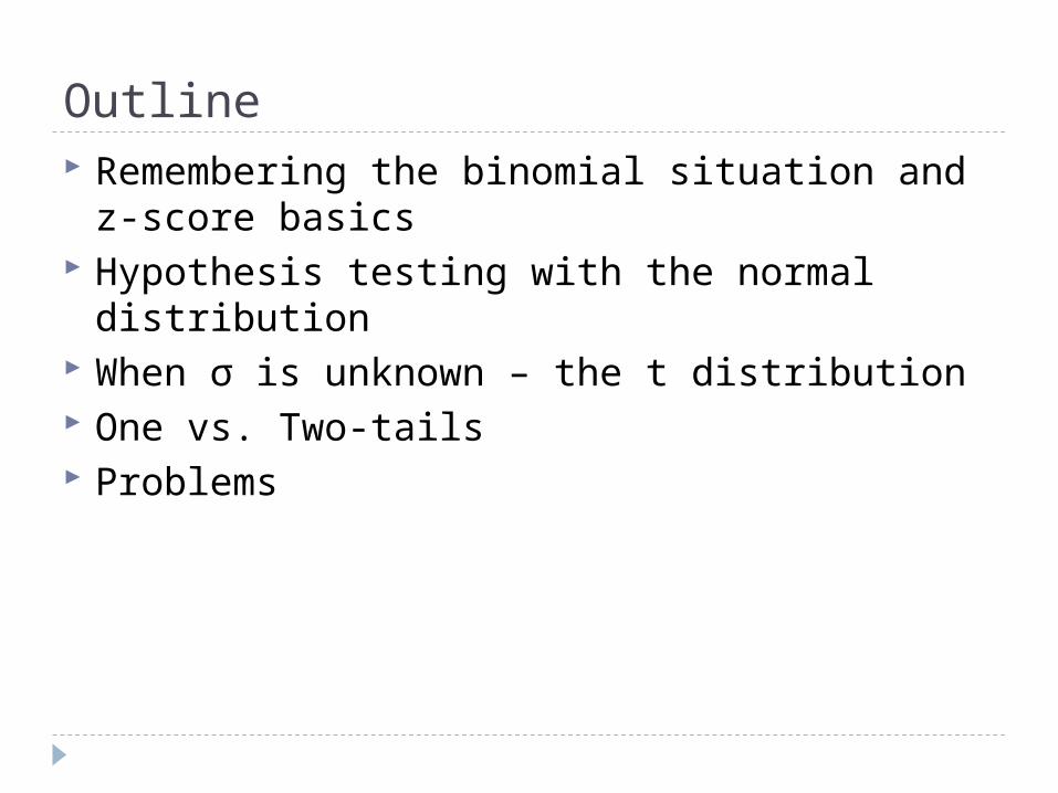
Outline Remembering the binomial situation and z-
score basics Hypothesis testing with the normal
distribution When σ is unknown – the t distribution One vs. Two-tails Problems
Recall the binomial
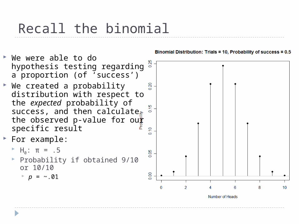
We were able to do hypothesis testing regarding a proportion (of ‘success’)
We created a probability distribution with respect to the expected probability of success, and then calculate the observed p-value for our specific result
For example: H0: π = .5 Probability if obtained 9/10 or
10/10 p = ~.01
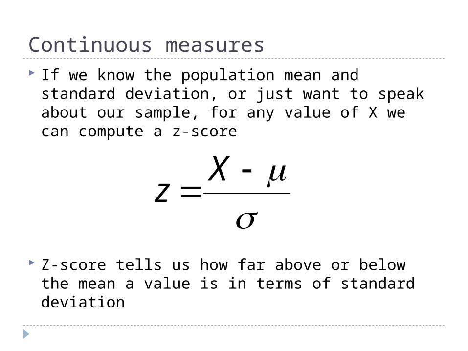
Continuous measures If we know the population mean and standard
deviation, or just want to speak about our sample, for any value of X we can compute a z-score
Z-score tells us how far above or below the mean a value is in terms of standard deviation
X
z
Hypothesis testing using the normal
X
Xz
orN
Xz
/
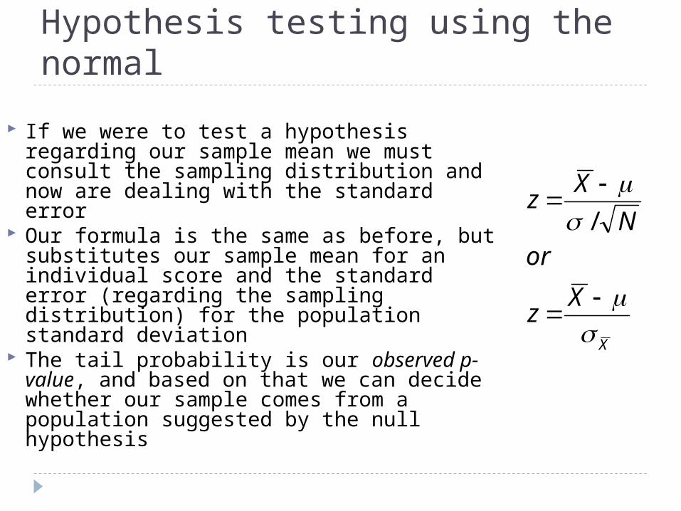
If we were to test a hypothesis regarding our sample mean we must consult the sampling distribution and now are dealing with the standard error
Our formula is the same as before, but substitutes our sample mean for an individual score and the standard error (regarding the sampling distribution) for the population standard deviation
The tail probability is our observed p-value, and based on that we can decide whether our sample comes from a population suggested by the null hypothesis
Conceptual summary thus far H0: μ = some value
Sample mean does not equal H0
But how different is it? Is it what we would typically expect due to
sampling variability or extreme enough to think that our sample does not come from such a population suggested by the null hypothesis?
Z to t In most situations we do not know However the sample standard deviation has
properties that make it a good estimate of the population value
We can use our sample standard deviation to estimate the population standard deviation
However, if we use the normal distribution probabilities, they would be incorrect
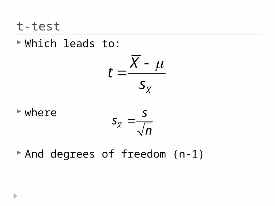
t-test Which leads to:
where
And degrees of freedom (n-1)
Xs
Xt
X
ss
n
Interpretation How many standard deviations away from the
population mean is my sample mean in terms of the sampling distribution of means
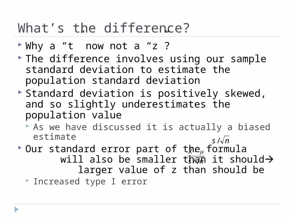
What’s the difference? Why a “t” now not a “z”? The difference involves using our sample
standard deviation to estimate the population standard deviation
Standard deviation is positively skewed, and so slightly underestimates the population value As we have discussed it is actually a biased
estimate Our standard error part of the formula
will also be smaller than it should larger value of z than should be Increased type I error
ns /
ns
X
/
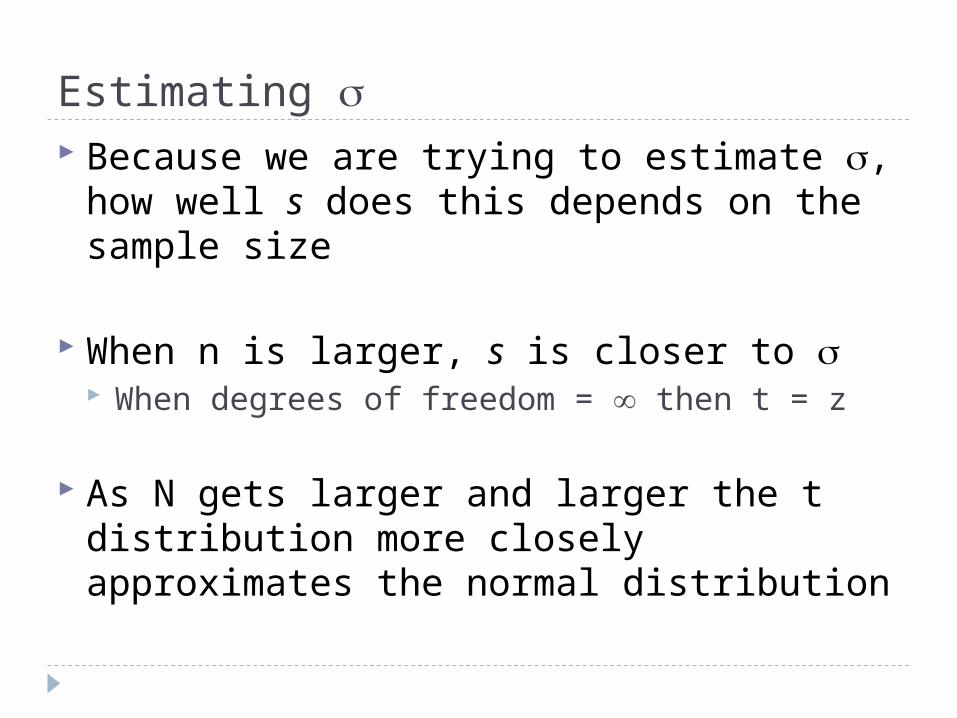
Estimating Because we are trying to estimate , how
well s does this depends on the sample size
When n is larger, s is closer to When degrees of freedom = then t = z
As N gets larger and larger the t distribution more closely approximates the normal distribution
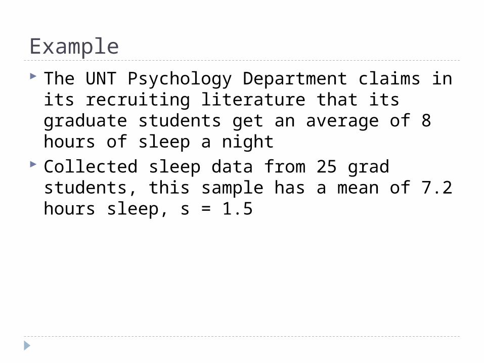
Example The UNT Psychology Department claims in its
recruiting literature that its graduate students get an average of 8 hours of sleep a night
Collected sleep data from 25 grad students, this sample has a mean of 7.2 hours sleep, s = 1.5
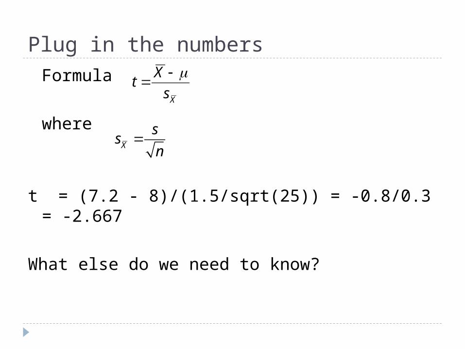
Plug in the numbersFormula
where
t = (7.2 - 8)/(1.5/sqrt(25)) = -0.8/0.3 = -2.667
What else do we need to know?
Xs
Xt
X
ss
n
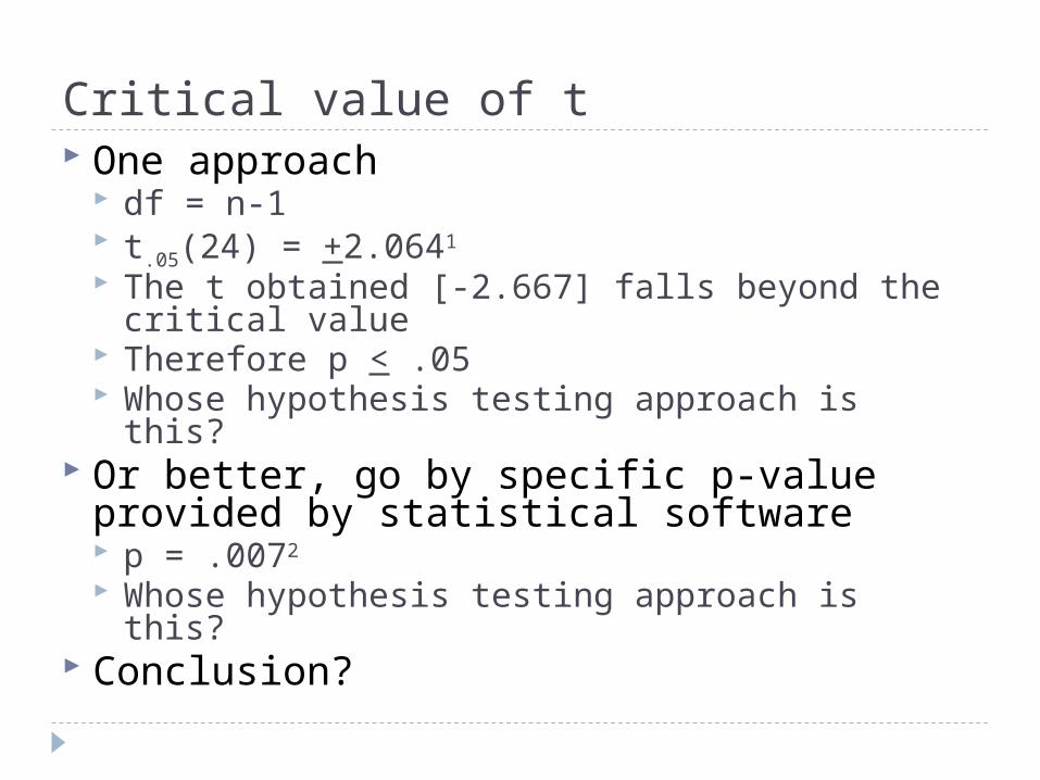
Critical value of t One approach
df = n-1 t.05(24) = +2.0641
The t obtained [-2.667] falls beyond the critical value
Therefore p < .05 Whose hypothesis testing approach is this?
Or better, go by specific p-value provided by statistical software p = .0072
Whose hypothesis testing approach is this? Conclusion?
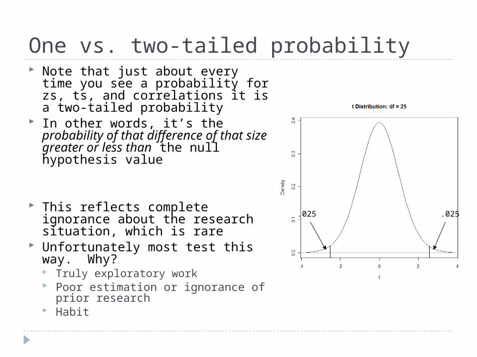
One vs. two-tailed probability Note that just about every time
you see a probability for zs, ts, and correlations it is a two-tailed probability
In other words, it’s the probability of that difference of that size greater or less than the null hypothesis value
This reflects complete ignorance about the research situation, which is rare
Unfortunately most test this way. Why? Truly exploratory work Poor estimation or ignorance of
prior research Habit
.025 .025
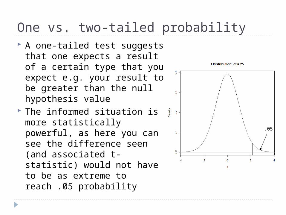
One vs. two-tailed probability A one-tailed test suggests
that one expects a result of a certain type that you expect e.g. your result to be greater than the null hypothesis value
The informed situation is more statistically powerful, as here you can see the difference seen (and associated t-statistic) would not have to be as extreme to reach .05 probability
.05
Your turn... The average grade from year to year in
undergrad statistics courses at UNT is an 81. This year the stats students (200 thus far) have an average of 83 w/ s = 10. Is this unusual?t.05(199)1= ? 2-tailed, i.e. probability associated with scores higher or lower than null. Before going in to this we would not have known whether they would be better or worse than the previous.t = ?p = ?Conclusion?
Problems with t Wilcox and others note that when we sample from
a non-normal population, assuming normality of the sampling distribution may be optimistic with small samples
Furthermore outliers have an influence on both the mean and sd used to calculate t Has a larger effect on variance, increasing type II
error due to std error increasing more so than the mean
This is not to say we throw the t-distribution out the window If normality can be assumed, it is appropriate
However, if we cannot meet the normality assumption we may have to try a different approach E.g. bootstrapping
Top Related