Chi-Square & F DistributionsCarolyn J. Anderson

EdPsych 580

Fall 2005

Chi-Square & F Distributions – p. 1/55

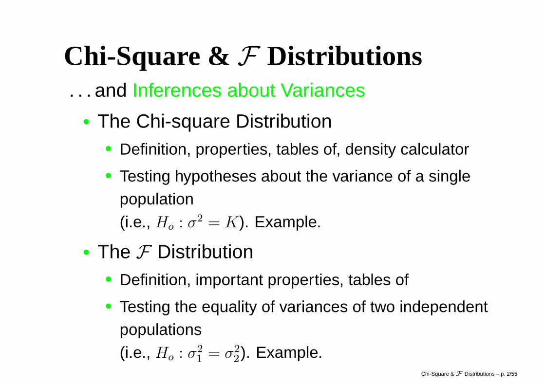
Chi-Square & F Distributions. . . and Inferences about Variances

• The Chi-square Distribution• Definition, properties, tables of, density calculator

• Testing hypotheses about the variance of a singlepopulation(i.e., Ho : σ2 = K). Example.

• The F Distribution• Definition, important properties, tables of

• Testing the equality of variances of two independentpopulations(i.e., Ho : σ2

1 = σ22). Example.

Chi-Square & F Distributions – p. 2/55

Chi-Square & F Distributions

. . . and Inferences about Variances• Comments regarding testing the homogeneity

of variance assumption of the twoindependent groups t–test (and ANOVA).

• Relationship among the Normal, t, χ2, and Fdistributions.

Chi-Square & F Distributions – p. 3/55

Chi-Square & F Distributions• Motivation. The normal and t distributions are

useful for tests of population means, but oftenwe may want to make inferences aboutpopulation variances.

• Examples:• Does the variance equal a particular value?

• Does the variance in one population equal thevariance in another population?

• Are individual differences greater in one populationthan another population?

• Are the variances in J populations all the same?

• Is the assumption of homogeneous variancesreasonable when doing a t–test (or ANOVA) of two

Chi-Square & F Distributions – p. 4/55

Chi-Square & F Distributions• To make statistical inferences about

populations variance(s), we need• χ2 −→ The Chi-square distribution (Greek

“chi”).• F−→ Named after Sir Ronald Fisher who

developed the main applications of F .

• The χ2 and F–distributions are used for manyproblems in addition to the ones listed above.

• They provide good approximations to a largeclass of sampling distributions that are noteasily determined.

Chi-Square & F Distributions – p. 5/55

The Big Five Theoretical Distributions

• The Big Five are Normal, Student’s t, χ2, F ,and the Binomial (π, n).

• Plan:• Introduce χ2 and then the F distributions.• Illustrate their uses for testing variances.• Summarize and describe the relationship

among the Normal, Student’s t, χ2 and F .

Chi-Square & F Distributions – p. 6/55

The Chi-Square Distributions• Suppose we have a population with scores Y

that are normally distributed with meanE(Y ) = µ and variance = var(Y ) = σ2 (i.e.,Y ∼ N (µ, σ2)).

• If we repeatedly take samples of size n = 1and for each “sample” compute

z2 =(Y − µ)2

σ2= squared standard score

• Define χ21 = z2

• What would the sampling distribution of χ21

look like?Chi-Square & F Distributions – p. 7/55

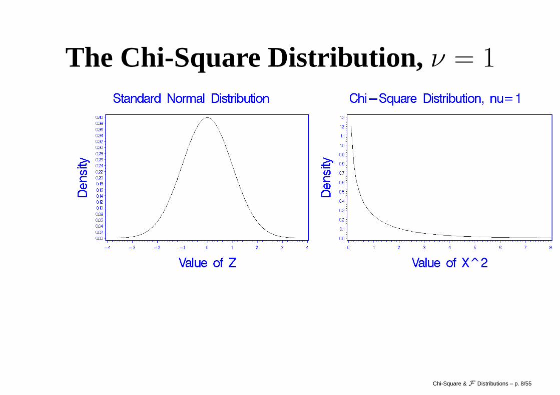
The Chi-Square Distribution, ν = 1

Chi-Square & F Distributions – p. 8/55

The Chi-Square Distribution, ν = 1

• χ21 are non-negative Real numbers

• Since 68% of values from N (0, 1) fall between−1 to 1, 68% of values from χ2

1 distributionmust be between 0 and 1.

• The chi-square distribution with ν = 1 is veryskewed.

Chi-Square & F Distributions – p. 9/55

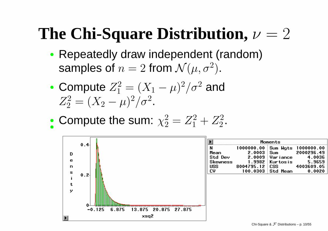
The Chi-Square Distribution, ν = 2

• Repeatedly draw independent (random)samples of n = 2 from N (µ, σ2).

• Compute Z21 = (X1 − µ)2/σ2 and

Z22 = (X2 − µ)2/σ2.

• Compute the sum: χ22 = Z2

1 + Z22 .•

Chi-Square & F Distributions – p. 10/55

The Chi-Square Distribution, ν = 2

• All value non-negative

• A little less skewed than χ21.

• The probability that χ22 falls in the range of 0

to 1 is smaller relative to that for χ21. . .

P (χ21 ≤ 1) = .68

P (χ22 ≤ 1) = .39

• Note that mean ≈ ν = 2. . . .

Chi-Square & F Distributions – p. 11/55

Chi-Square Distributions• Generalize: For n independent observations

from a N (µ, σ2), the sum of the squaredstandard scores has a Chi-square distributionwith n degrees of freedom.

• Chi–squared distribution only depends ondegrees of freedom, which in turn dependson sample size n.

• The standard scores are computed usingpopulation µ and σ2; however, we usuallydon’t know what µ and σ2 equal. When µ andσ2 are estimated from the sampled data, thedegrees of freedom are less than n.

Chi-Square & F Distributions – p. 12/55

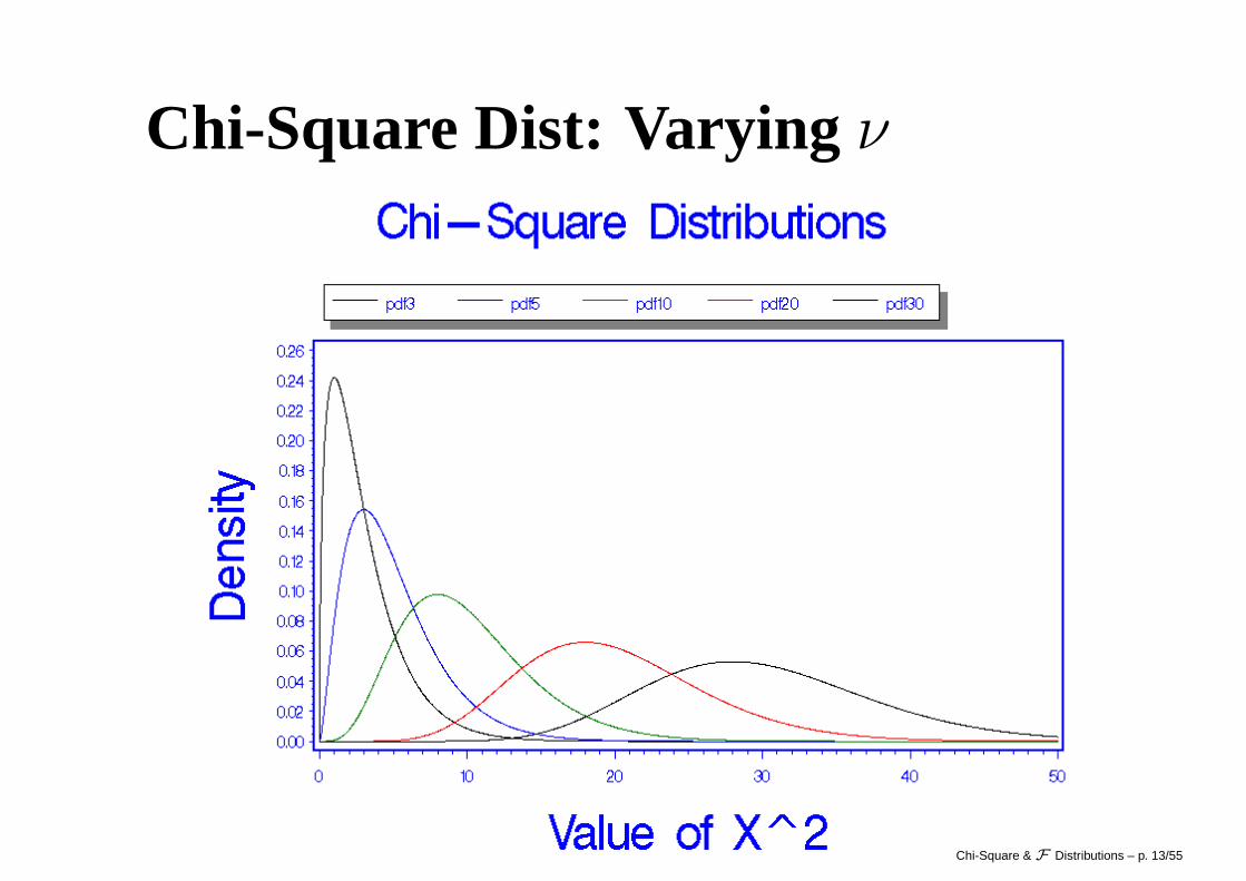
Chi-Square Dist: Varying ν

Chi-Square & F Distributions – p. 13/55

Properties of Family of χ2 Distributions• They are all positively skewed.• As ν gets larger, the degree of skew

decreases.• As ν gets very large, χ2

ν approaches thenormal distribution.

Why? The Central Limit Theorem (for sums):Consider a random sample of size n from a populationdistribution having mean µ and variance σ2. If n issufficiently large, then the distribution of

∑ni=1 Yi is

approximately normal with mean nµ and variance σ2.

Chi-Square & F Distributions – p. 14/55

Properties of Family of χ2 Distributions

• E(χ2ν) = mean = ν = degrees of freedom.

• E[(χ2ν − E(χ2

ν))2] = var(χ2

ν) = 2ν.

• Mode of χ2ν is at value ν − 2 (for ν ≥ 2).

• Median is approximately = (3ν − 2)/3 (forν ≥ 2).

Chi-Square & F Distributions – p. 15/55

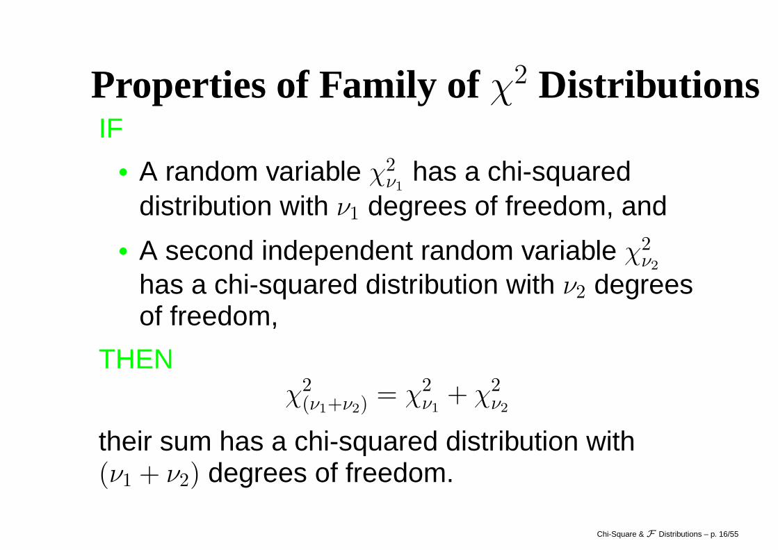
Properties of Family of χ2 DistributionsIF

• A random variable χ2ν1

has a chi-squareddistribution with ν1 degrees of freedom, and

• A second independent random variable χ2ν2

has a chi-squared distribution with ν2 degreesof freedom,

THENχ2

(ν1+ν2)= χ2

ν1+ χ2

ν2

their sum has a chi-squared distribution with(ν1 + ν2) degrees of freedom.

Chi-Square & F Distributions – p. 16/55

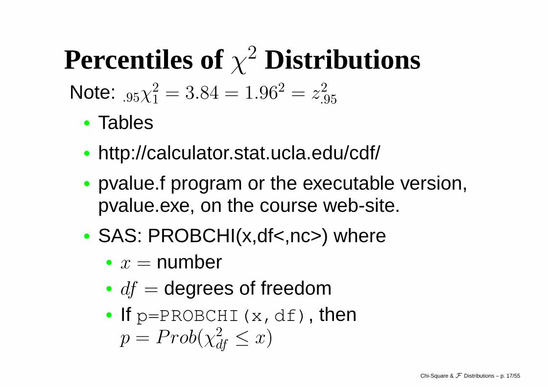
Percentiles ofχ2 DistributionsNote: .95χ

21 = 3.84 = 1.962 = z2

.95

• Tables• http://calculator.stat.ucla.edu/cdf/• pvalue.f program or the executable version,

pvalue.exe, on the course web-site.• SAS: PROBCHI(x,df<,nc>) where

• x = number• df = degrees of freedom• If p=PROBCHI(x,df), then

p = Prob(χ2df ≤ x)

Chi-Square & F Distributions – p. 17/55

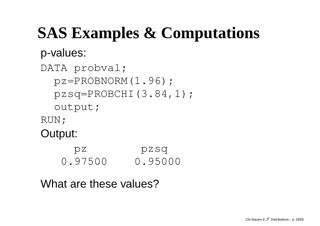
SAS Examples & Computationsp-values:DATA probval;pz=PROBNORM(1.96);pzsq=PROBCHI(3.84,1);output;

RUN;Output:

pz pzsq0.97500 0.95000

What are these values?

Chi-Square & F Distributions – p. 18/55

SAS Examples & Computations

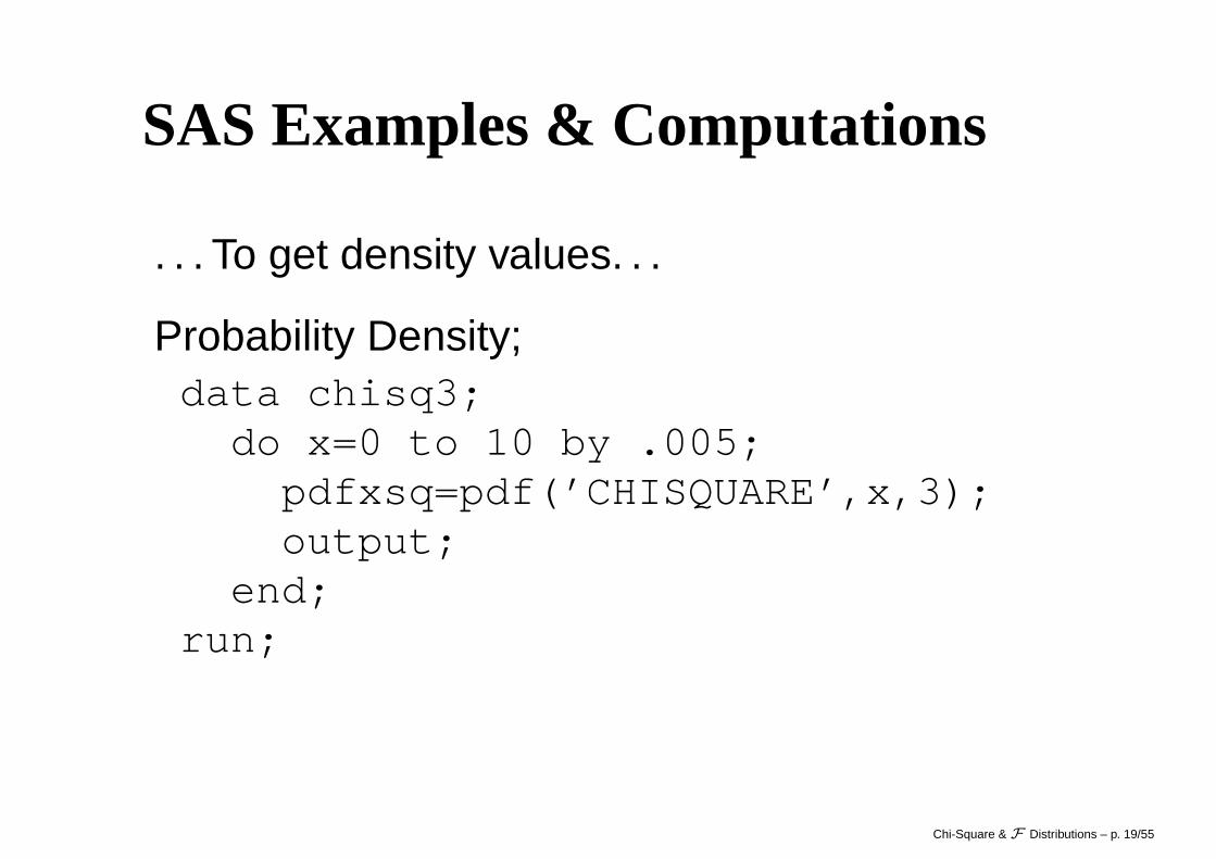
. . . To get density values. . .

Probability Density;data chisq3;do x=0 to 10 by .005;

pdfxsq=pdf(’CHISQUARE’,x,3);output;

end;run;

Chi-Square & F Distributions – p. 19/55

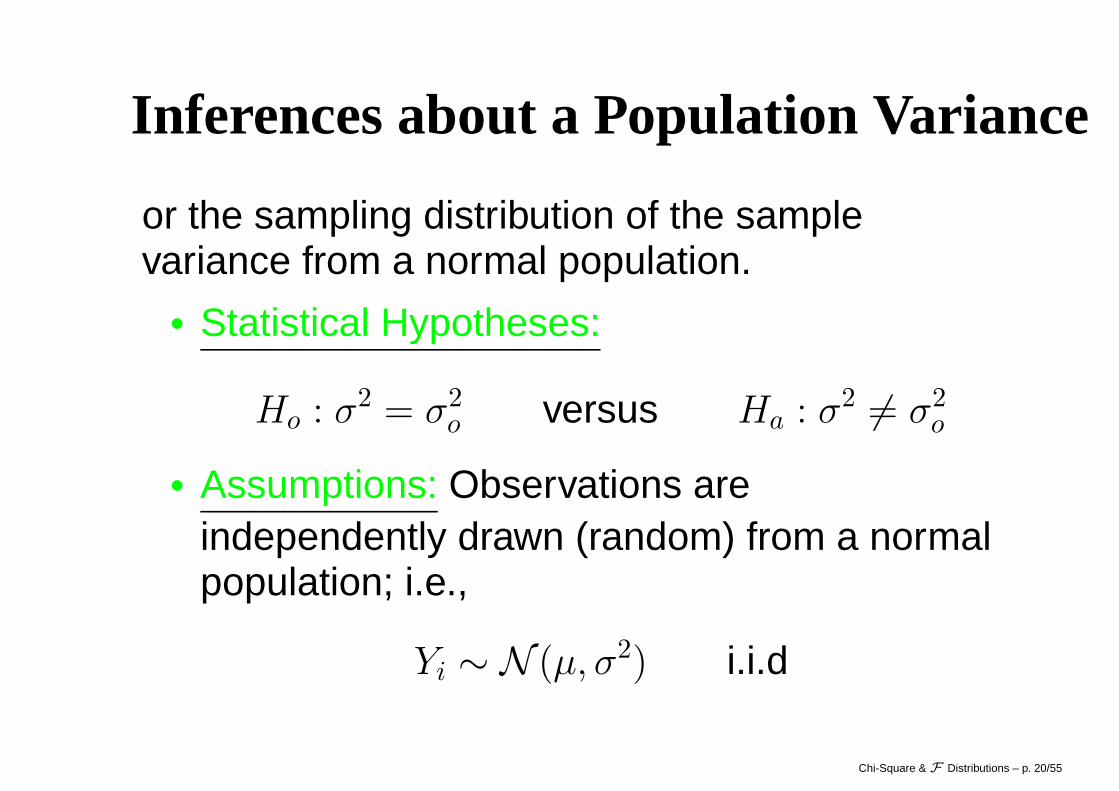
Inferences about a Population Variance

or the sampling distribution of the samplevariance from a normal population.

• Statistical Hypotheses:

Ho : σ2 = σ2o versus Ha : σ2 6= σ2

o

• Assumptions: Observations areindependently drawn (random) from a normalpopulation; i.e.,

Yi ∼ N (µ, σ2) i.i.d

Chi-Square & F Distributions – p. 20/55

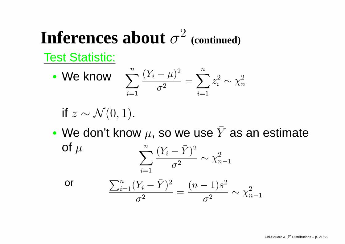
Inferences aboutσ2(continued)

Test Statistic:• We know

n∑

i=1

(Yi − µ)2

σ2=

n∑

i=1

z2i ∼ χ2

n

if z ∼ N (0, 1).

• We don’t know µ, so we use Y as an estimateof µ n

∑

i=1

(Yi − Y )2

σ2∼ χ2

n−1

or ∑ni=1(Yi − Y )2

σ2=

(n − 1)s2

σ2∼ χ2

n−1

Chi-Square & F Distributions – p. 21/55

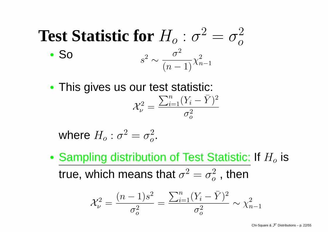
Test Statistic for Ho : σ2 = σ2o

• So s2 ∼ σ2

(n − 1)χ2

n−1

• This gives us our test statistic:

X 2ν =

∑ni=1(Yi − Y )2

σ2o

where Ho : σ2 = σ2o.

• Sampling distribution of Test Statistic: If Ho is

true, which means that σ2 = σ2o , then

X 2ν =

(n − 1)s2

σ2o

=

∑ni=1(Yi − Y )2

σ2o

∼ χ2n−1

Chi-Square & F Distributions – p. 22/55

Decision and Conclusion,Ho : σ2 = σ2o

• Decision: Compare the obtained test statisticto the chi-squared distribution with ν = n − 1degrees of freedom.

or find the p-value of the test statistic andcompare to α.

• Interpretation/Conclusion: What does thedecision mean in terms of what you’reinvestigating?

Chi-Square & F Distributions – p. 23/55

Example ofHo : σ2 = σ2o

• High School and Beyond: Is the variance ofmath scores of students from private schoolsequal to 100?

• Statistical Hypotheses:

Ho : σ2 = 100 versus Ha : σ2 6= 100

• Assumptions: Math scores are independentand normally distributed in the population ofhigh school seniors who attend privateschools and the observations areindependent.

Chi-Square & F Distributions – p. 24/55

Example ofHo : σ2 = σ2o (continued)

• Test Statistic: n = 94, s2 = 67.16, and setα = .10.

X 2 =(n − 1)s2

σ2=

(94 − 1)(67.16)

100= 62.46

with ν = (94 − 1) = 93.• Sampling Distribution of the Test Statistic:

Chi-square with ν = 93.

Critical values: .05χ293 = 71.76 & .95χ

293 = 116.51.

Chi-Square & F Distributions – p. 25/55

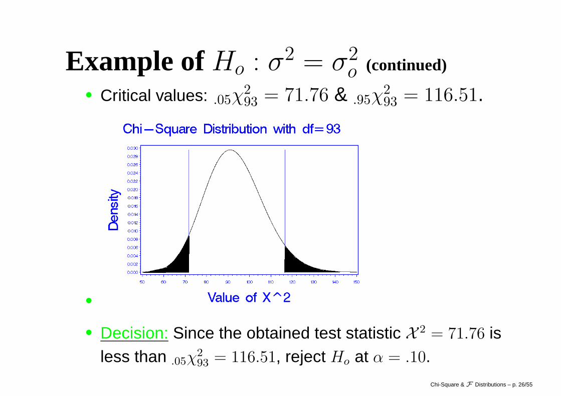
Example ofHo : σ2 = σ2o (continued)

• Critical values: .05χ293 = 71.76 & .95χ

293 = 116.51.

•

• Decision: Since the obtained test statistic X 2 = 71.76 isless than .05χ

293 = 116.51, reject Ho at α = .10.

Chi-Square & F Distributions – p. 26/55

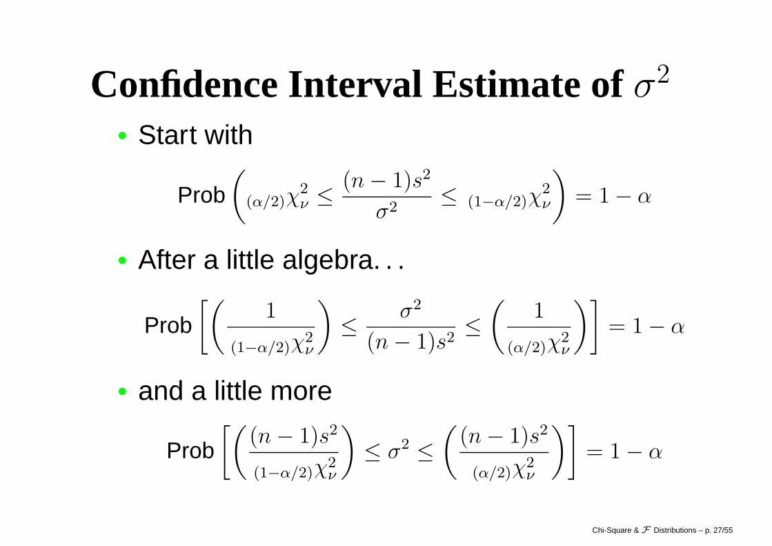
Confidence Interval Estimate ofσ2

• Start with

Prob(

(α/2)χ2ν ≤ (n − 1)s2

σ2≤ (1−α/2)χ

2ν

)

= 1 − α

• After a little algebra. . .

Prob[(

1

(1−α/2)χ2ν

)

≤ σ2

(n − 1)s2≤

(

1

(α/2)χ2ν

)]

= 1 − α

• and a little more

Prob[(

(n − 1)s2

(1−α/2)χ2ν

)

≤ σ2 ≤(

(n − 1)s2

(α/2)χ2ν

)]

= 1 − α

Chi-Square & F Distributions – p. 27/55

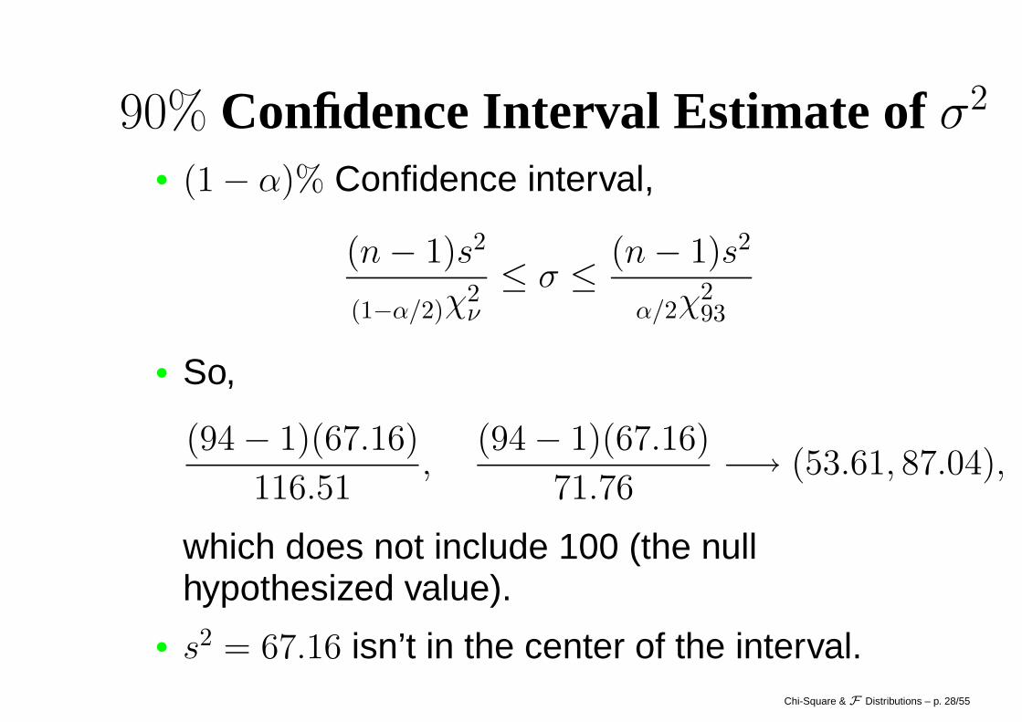
90% Confidence Interval Estimate ofσ2

• (1 − α)% Confidence interval,

(n − 1)s2

(1−α/2)χ2ν

≤ σ ≤ (n − 1)s2

α/2χ293

• So,

(94 − 1)(67.16)

116.51,

(94 − 1)(67.16)

71.76−→ (53.61, 87.04),

which does not include 100 (the nullhypothesized value).

• s2 = 67.16 isn’t in the center of the interval.Chi-Square & F Distributions – p. 28/55

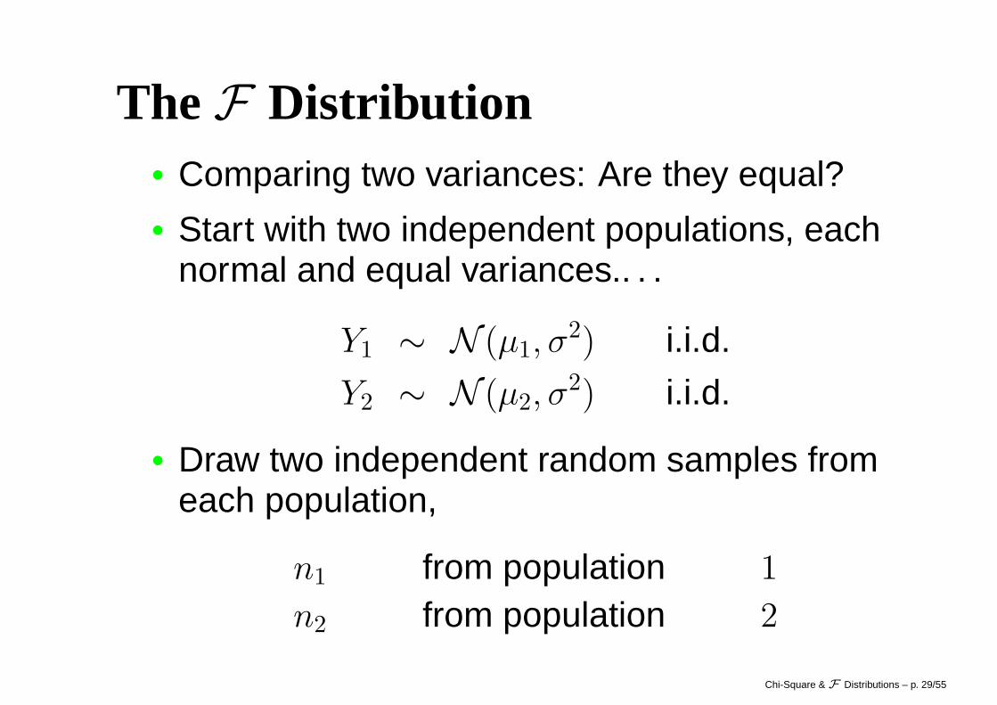
TheF Distribution• Comparing two variances: Are they equal?• Start with two independent populations, each

normal and equal variances.. . .

Y1 ∼ N (µ1, σ2) i.i.d.

Y2 ∼ N (µ2, σ2) i.i.d.

• Draw two independent random samples fromeach population,

n1 from population 1

n2 from population 2

Chi-Square & F Distributions – p. 29/55

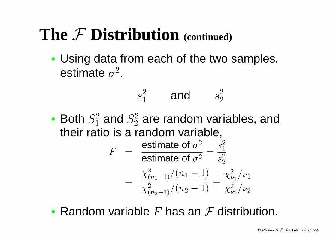
TheF Distribution (continued)

• Using data from each of the two samples,estimate σ2.

s21 and s2

2

• Both S21 and S2

2 are random variables, andtheir ratio is a random variable,

F =estimate of σ2

estimate of σ2=

s21

s22

=χ2

(n1−1)/(n1 − 1)

χ2(n2−1)/(n2 − 1)

=χ2

ν1/ν1

χ2ν2

/ν2

• Random variable F has an F distribution.Chi-Square & F Distributions – p. 30/55

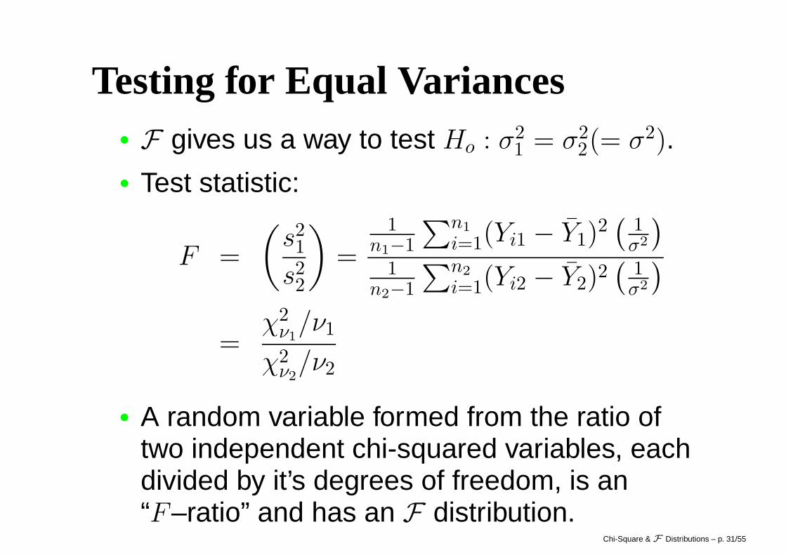
Testing for Equal Variances• F gives us a way to test Ho : σ2

1 = σ22(= σ2).

• Test statistic:

F =

(

s21

s22

)

=1

n1−1

∑n1

i=1(Yi1 − Y1)2(

1σ2

)

1n2−1

∑n2

i=1(Yi2 − Y2)2(

1σ2

)

=χ2

ν1/ν1

χ2ν2

/ν2

• A random variable formed from the ratio oftwo independent chi-squared variables, eachdivided by it’s degrees of freedom, is an“F–ratio” and has an F distribution.

Chi-Square & F Distributions – p. 31/55

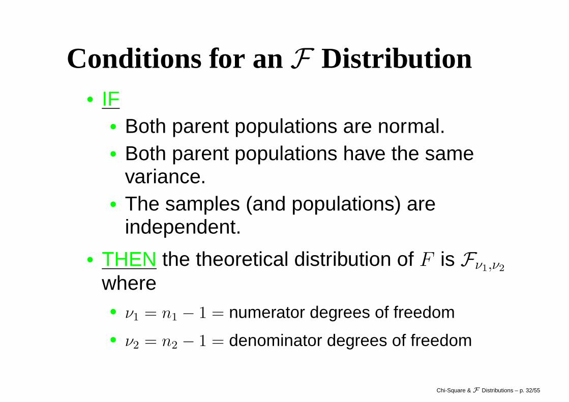
Conditions for an F Distribution• IF

• Both parent populations are normal.• Both parent populations have the same

variance.• The samples (and populations) are

independent.

• THEN the theoretical distribution of F is Fν1,ν2

where• ν1 = n1 − 1 = numerator degrees of freedom

• ν2 = n2 − 1 = denominator degrees of freedom

Chi-Square & F Distributions – p. 32/55

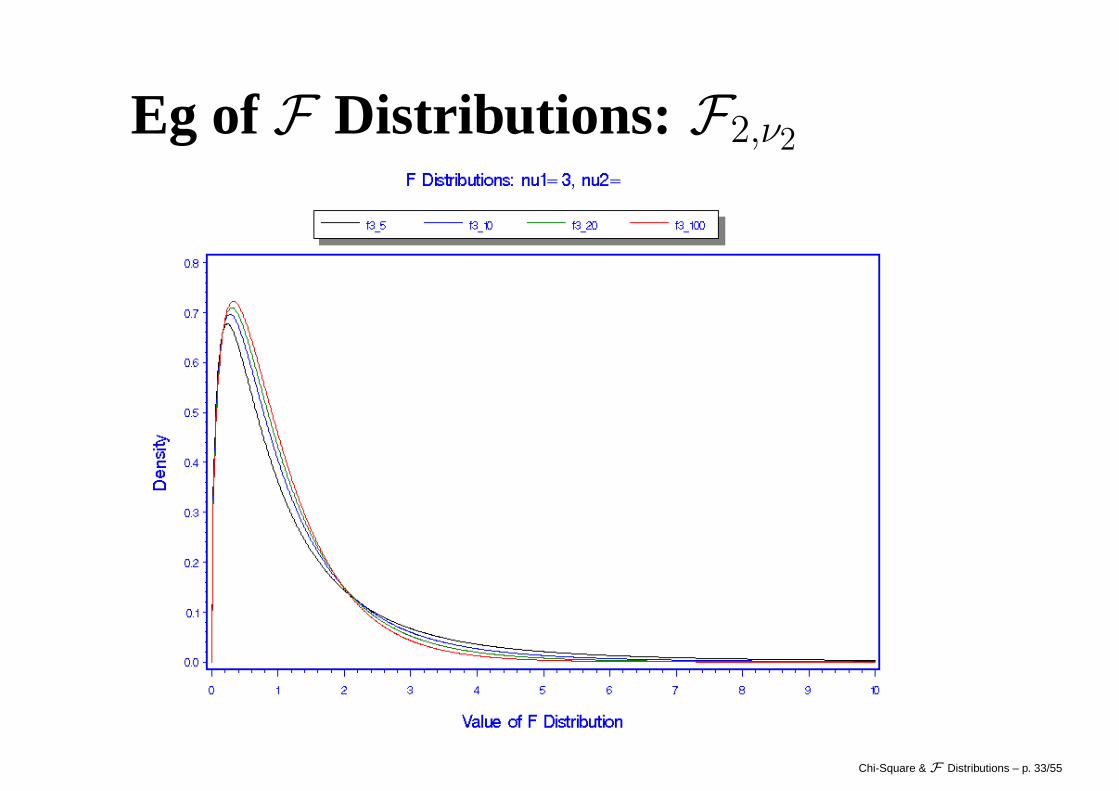
Eg ofF Distributions: F2,ν2

Chi-Square & F Distributions – p. 33/55

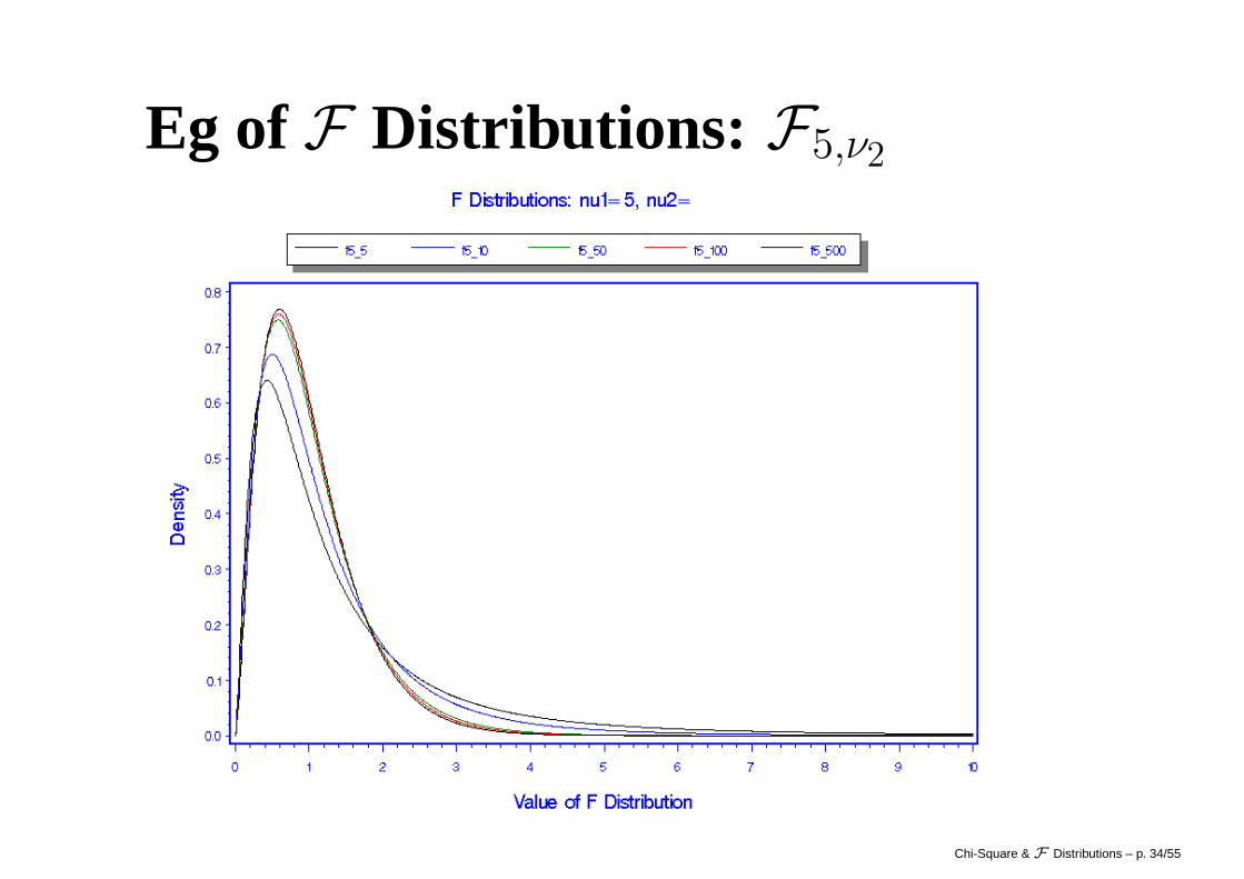
Eg ofF Distributions: F5,ν2

Chi-Square & F Distributions – p. 34/55

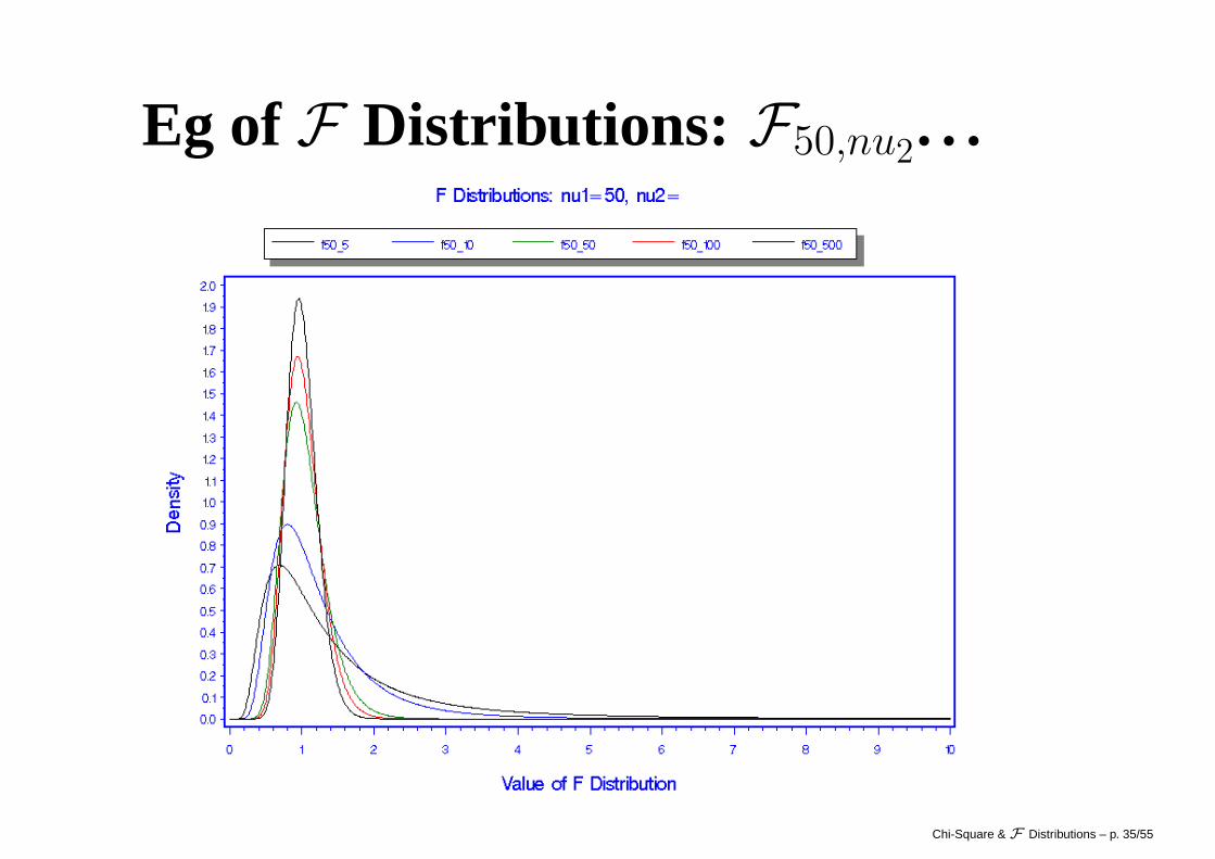
Eg ofF Distributions: F50,nu2. . .

Chi-Square & F Distributions – p. 35/55

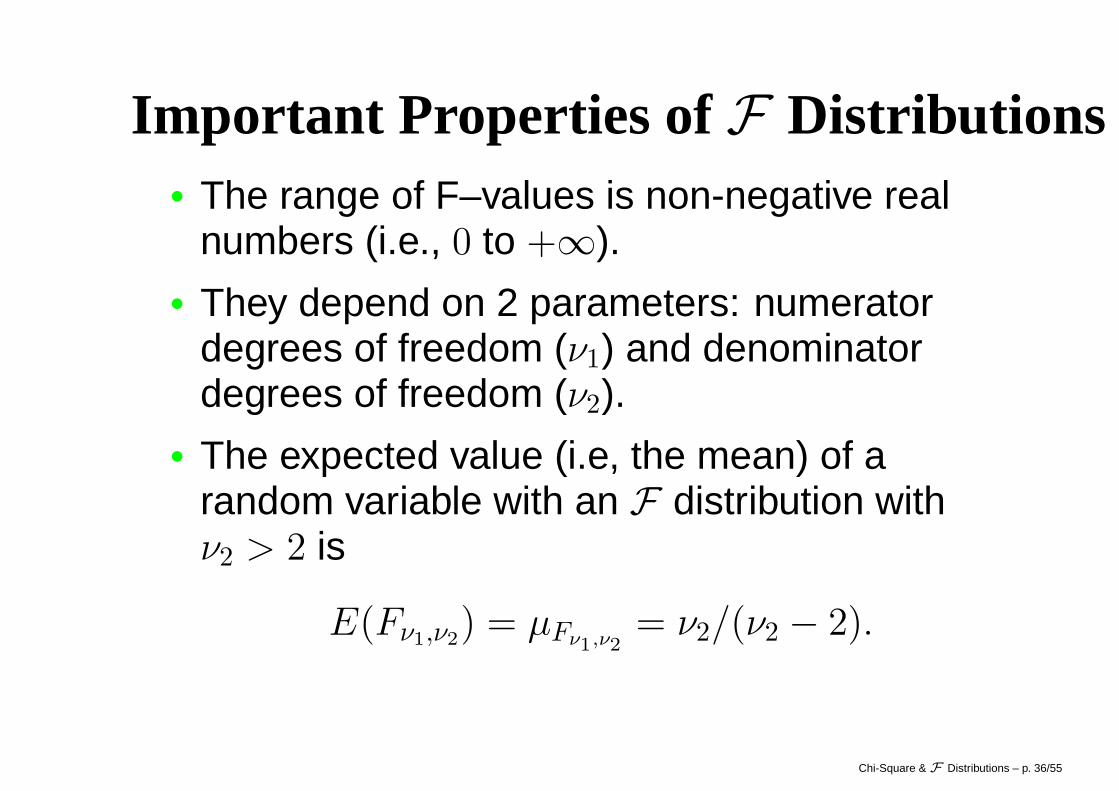
Important Properties of F Distributions• The range of F–values is non-negative real

numbers (i.e., 0 to +∞).• They depend on 2 parameters: numerator

degrees of freedom (ν1) and denominatordegrees of freedom (ν2).

• The expected value (i.e, the mean) of arandom variable with an F distribution withν2 > 2 is

E(Fν1,ν2) = µFν1,ν2

= ν2/(ν2 − 2).

Chi-Square & F Distributions – p. 36/55

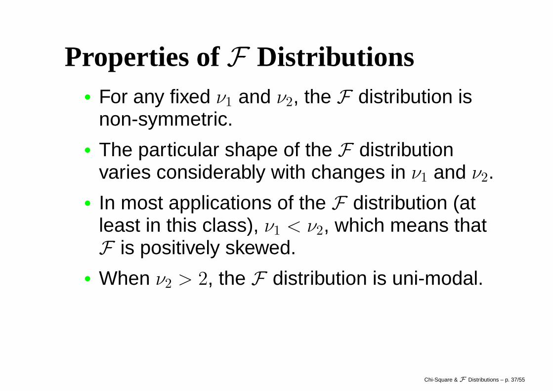
Properties ofF Distributions• For any fixed ν1 and ν2, the F distribution is

non-symmetric.• The particular shape of the F distribution

varies considerably with changes in ν1 and ν2.• In most applications of the F distribution (at

least in this class), ν1 < ν2, which means thatF is positively skewed.

• When ν2 > 2, the F distribution is uni-modal.

Chi-Square & F Distributions – p. 37/55

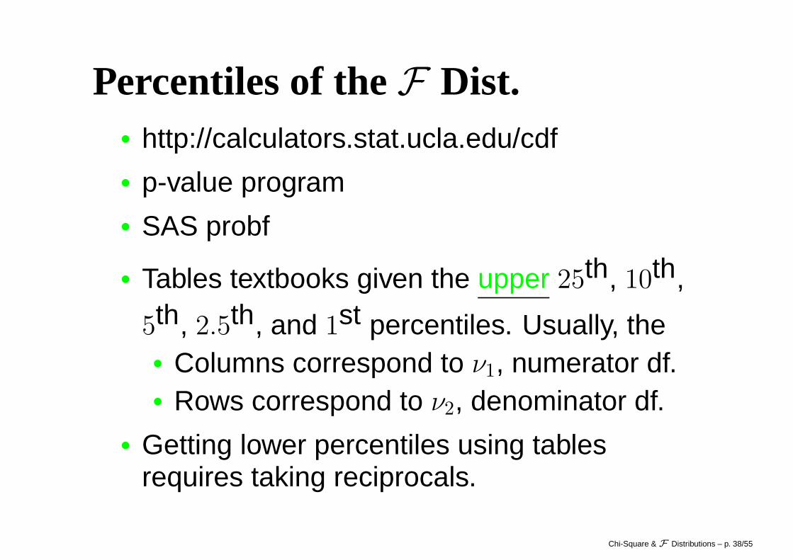
Percentiles of theF Dist.• http://calculators.stat.ucla.edu/cdf• p-value program• SAS probf

• Tables textbooks given the upper 25th, 10th,

5th, 2.5th, and 1st percentiles. Usually, the• Columns correspond to ν1, numerator df.• Rows correspond to ν2, denominator df.

• Getting lower percentiles using tablesrequires taking reciprocals.

Chi-Square & F Distributions – p. 38/55

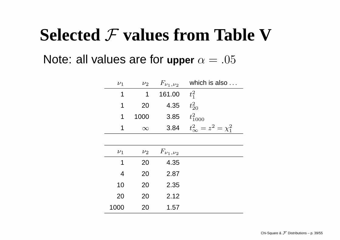
SelectedF values from Table VNote: all values are for upper α = .05

ν1 ν2 Fν1,ν2which is also . . .

1 1 161.00 t21

1 20 4.35 t220

1 1000 3.85 t21000

1 ∞ 3.84 t2∞

= z2 = χ2

1

ν1 ν2 Fν1,ν2

1 20 4.35

4 20 2.87

10 20 2.35

20 20 2.12

1000 20 1.57

Chi-Square & F Distributions – p. 39/55

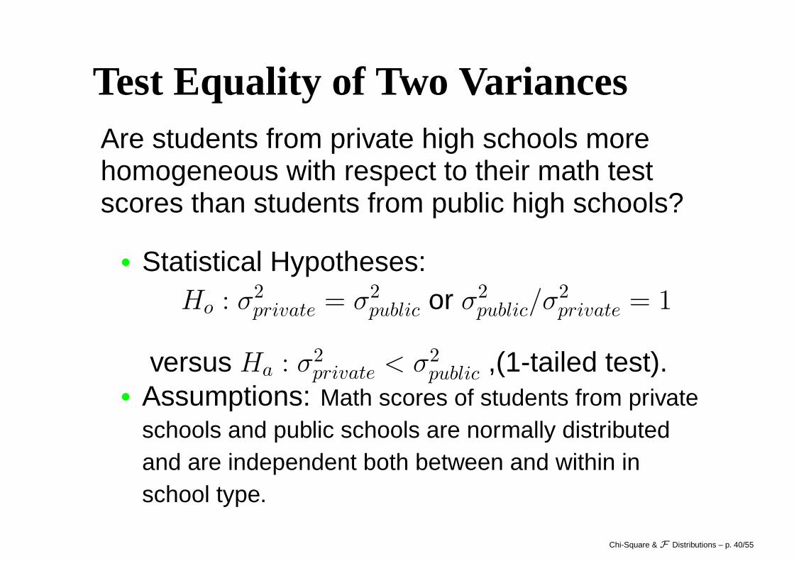
Test Equality of Two VariancesAre students from private high schools morehomogeneous with respect to their math testscores than students from public high schools?

• Statistical Hypotheses:Ho : σ2

private = σ2public or σ2

public/σ2private = 1

versus Ha : σ2private < σ2

public ,(1-tailed test).• Assumptions: Math scores of students from private

schools and public schools are normally distributedand are independent both between and within inschool type.

Chi-Square & F Distributions – p. 40/55

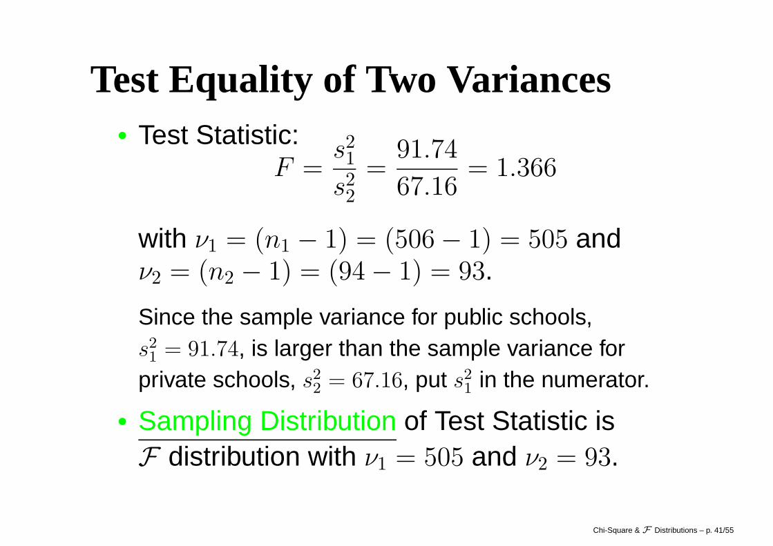
Test Equality of Two Variances• Test Statistic:

F =s21

s22

=91.74

67.16= 1.366

with ν1 = (n1 − 1) = (506 − 1) = 505 andν2 = (n2 − 1) = (94 − 1) = 93.

Since the sample variance for public schools,s21 = 91.74, is larger than the sample variance for

private schools, s22 = 67.16, put s2

1 in the numerator.

• Sampling Distribution of Test Statistic isF distribution with ν1 = 505 and ν2 = 93.

Chi-Square & F Distributions – p. 41/55

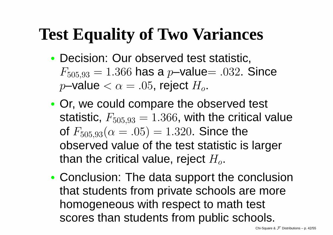
Test Equality of Two Variances• Decision: Our observed test statistic,

F505,93 = 1.366 has a p–value= .032. Sincep–value < α = .05, reject Ho.

• Or, we could compare the observed teststatistic, F505,93 = 1.366, with the critical valueof F505,93(α = .05) = 1.320. Since theobserved value of the test statistic is largerthan the critical value, reject Ho.

• Conclusion: The data support the conclusionthat students from private schools are morehomogeneous with respect to math testscores than students from public schools.

Chi-Square & F Distributions – p. 42/55

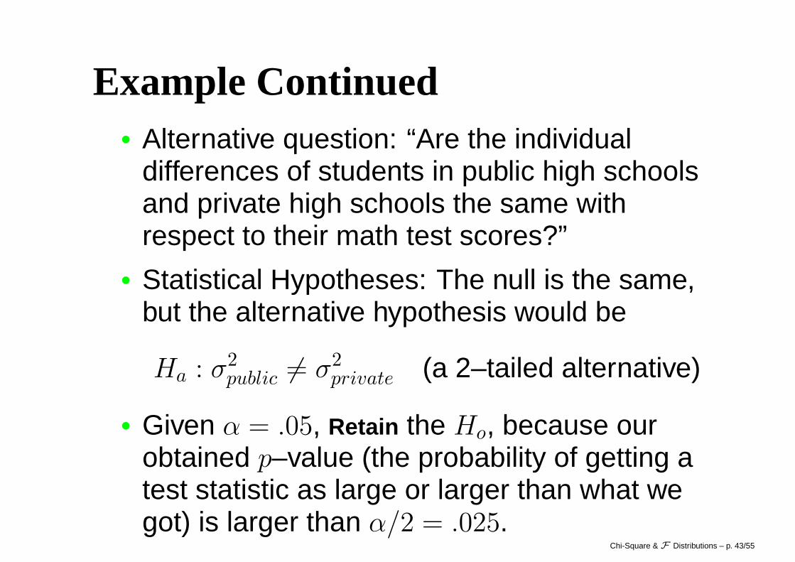
Example Continued• Alternative question: “Are the individual

differences of students in public high schoolsand private high schools the same withrespect to their math test scores?”

• Statistical Hypotheses: The null is the same,but the alternative hypothesis would be

Ha : σ2public 6= σ2

private (a 2–tailed alternative)

• Given α = .05, Retain the Ho, because ourobtained p–value (the probability of getting atest statistic as large or larger than what wegot) is larger than α/2 = .025.

Chi-Square & F Distributions – p. 43/55

Example Continued

• Given α = .05, Retain the Ho, because ourobtained p–value (the probability of getting atest statistic as large or larger than what wegot) is larger than α/2 = .025.

• Or the rejection region (critical value) wouldbe any F–statistic greater thanF505,93(α = .025) = 1.393.

• Point: This is a case where the choicebetween a 1 and 2 tailed test leads to differentdecisions regarding the null hypothesis.

Chi-Square & F Distributions – p. 44/55

Test for Homogeneity of Variances

Ho : σ21 = σ2

2 = . . . = σ2J

• These include• Hartley’s Fmax test• Bartlett’s test• One regarding variances of paired

comparisons.• You should know that they exist; we won’t go

over them in this class. Such tests are not asimportant as they once (thought) they were.

Chi-Square & F Distributions – p. 45/55

Test for Homogeneity of Variances• Old View: Testing the equality of variances

should be a preliminary to doing independentt-tests (or ANOVA).

• Newer View:• Homogeneity of variance is required for small

samples, which is when tests of homogeneousvariances do not work well. With large samples, wedon’t have to assume σ2

1 = σ22.

• Test critically depends on population normality.

• If n1 = n2, t-tests are robust.

Chi-Square & F Distributions – p. 46/55

Test for Homogeneity of Variances• For small or moderate samples and there’s

concern with possible heterogeneity −→perform a Quasi-t test.

• In an experimental settings where you havecontrol over the number of subjects and theirassignment to groups/conditions/etc. −→equal sample sizes.

• In non-experimental settings where you havesimilar numbers of participants per group, ttest is pretty robust.

Chi-Square & F Distributions – p. 47/55

Relationship betweenz, tν, χ2ν, andFν1,ν2

. . . and the central importance of the normaldistribution.

• Normal, Student’s tν, χ2ν, and Fν1,ν2

are alltheoretical distributions.

• We don’t ever actually take vast (infinite)numbers of samples from populations.

• The distributions are derived based onmathematical logic statements of the form

IF . . . . . . . . . Then . . . . . . . . .

Chi-Square & F Distributions – p. 48/55

Derivation of Distributions

• Example• IF we draw independent random samples of size

(large) n from a population and compute the meanY and repeat this process many, many, many, manytimes,

• THEN Y is approximately normal.

• Assumptions are part of the “if” part, the conditionsused to deduce sampling distribution of statistics.

• The t, χ2 and F distributions all depend on normal“parent” population.

Chi-Square & F Distributions – p. 49/55

Chi-Square Distribution

• χ2ν = sum of independent squared normal

random variables with mean µ = 0 andvariance σ2 = 1 (i.e., “standard normal”random variables).

χ2ν =

n∑

i=1

z2i where zi ∼ N (0, 1)

• Based on the Central Limit Theorem, the“limit” of the χ2

ν distribution (i.e., n → ∞) isnormal.

Chi-Square & F Distributions – p. 50/55

TheF Distribution• Fν1,ν2

= ratio of two independent chi-squaredrandom variables each divided by theirrespective degrees of freedom.

Fν1,ν2=

χ2ν1

/ν1

χ2ν2

/ν2

• Since χ2ν ’s depend on the normal distribution,

the F distribution also depends on the normaldistribution.

• The “limiting” distribution of Fν1,ν2as ν2 → ∞

is χ2ν1

/ν1.. . . . . . because as ν2 → ∞,χ2

ν2/ν2 → 1.

Chi-Square & F Distributions – p. 51/55

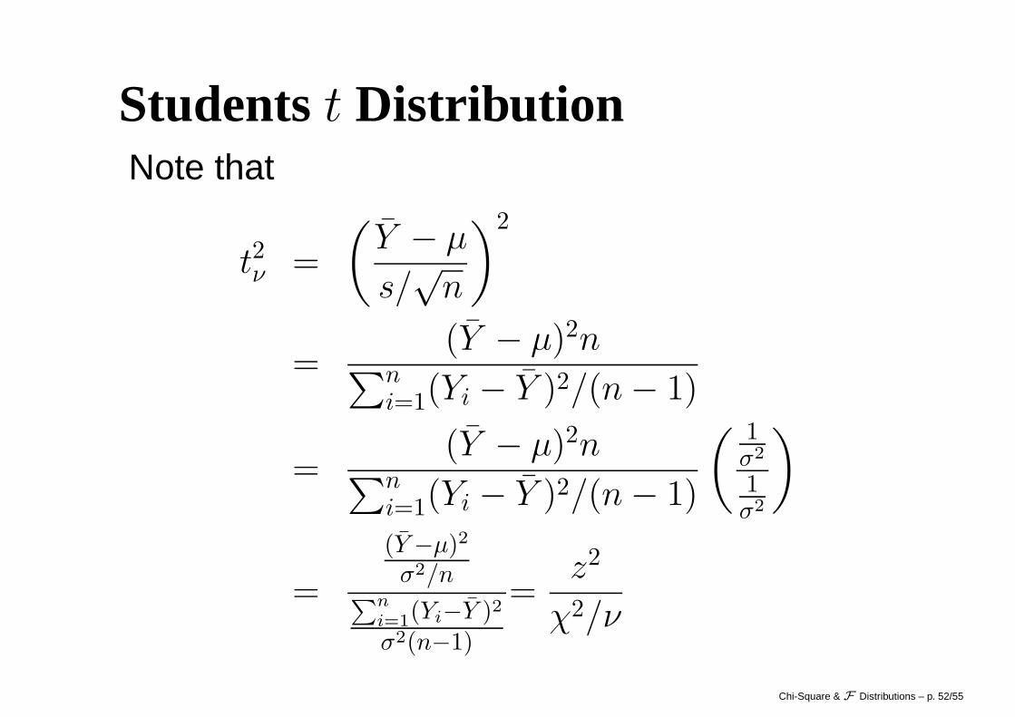
Studentst DistributionNote that

t2ν =

(

Y − µ

s/√

n

)2

=(Y − µ)2n

∑ni=1(Yi − Y )2/(n − 1)

=(Y − µ)2n

∑ni=1(Yi − Y )2/(n − 1)

( 1σ2

1σ2

)

=

(Y −µ)2

σ2/n∑n

i=1(Yi−Y )2

σ2(n−1)

=z2

χ2/ν

Chi-Square & F Distributions – p. 52/55

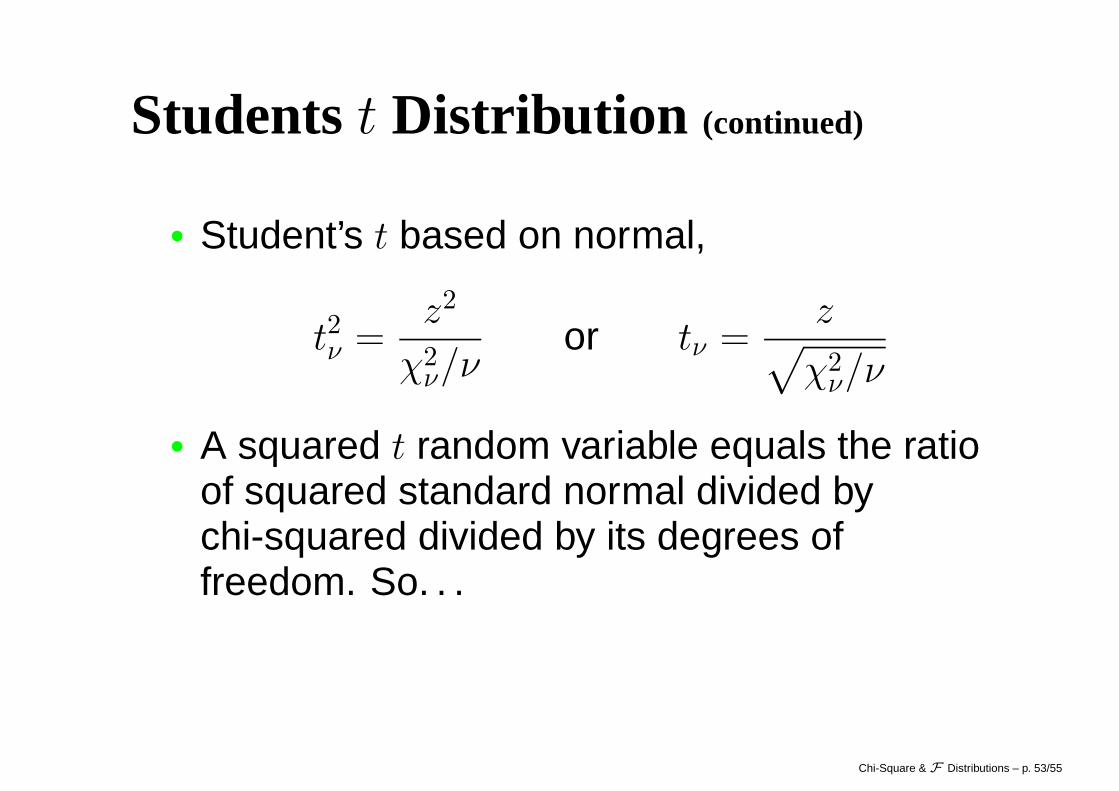
Studentst Distribution (continued)

• Student’s t based on normal,

t2ν =z2

χ2ν/ν

or tν =z

√

χ2ν/ν

• A squared t random variable equals the ratioof squared standard normal divided bychi-squared divided by its degrees offreedom. So. . .

Chi-Square & F Distributions – p. 53/55

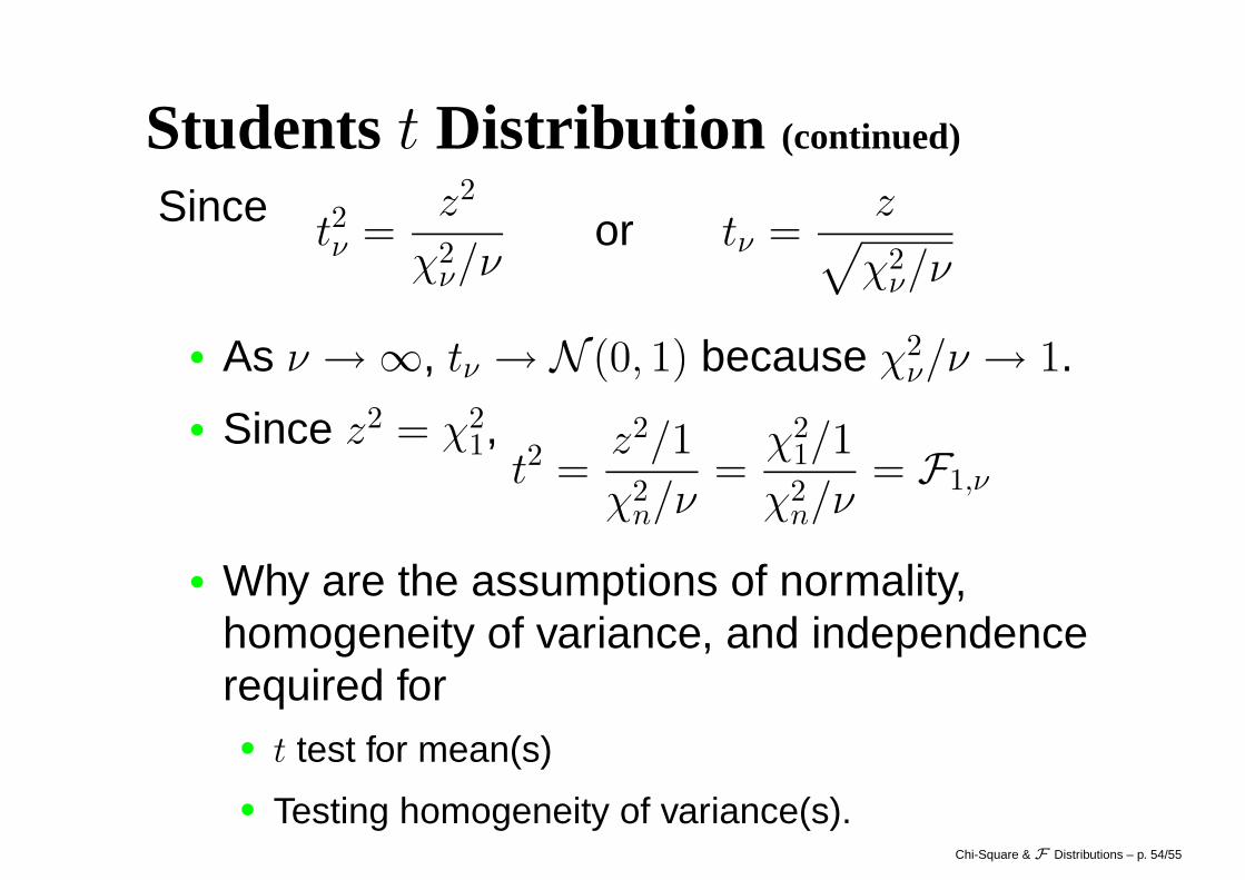
Studentst Distribution (continued)

Sincet2ν =

z2

χ2ν/ν

or tν =z

√

χ2ν/ν

• As ν → ∞, tν → N (0, 1) because χ2ν/ν → 1.

• Since z2 = χ21,

t2 =z2/1

χ2n/ν

=χ2

1/1

χ2n/ν

= F1,ν

• Why are the assumptions of normality,homogeneity of variance, and independencerequired for• t test for mean(s)

• Testing homogeneity of variance(s).Chi-Square & F Distributions – p. 54/55

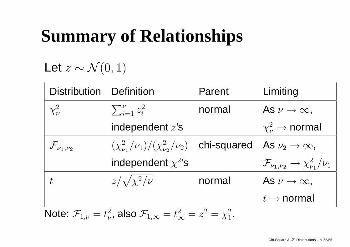
Summary of Relationships

Let z ∼ N (0, 1)

Distribution Definition Parent Limiting

χ2ν

∑νi=1 z2

i normal As ν → ∞,

independent z’s χ2ν → normal

Fν1,ν2(χ2

ν1/ν1)/(χ

2ν2

/ν2) chi-squared As ν2 → ∞,

independent χ2’s Fν1,ν2→ χ2

ν1/ν1

t z/√

χ2/ν normal As ν → ∞,

t → normal

Note: F1,ν = t2ν , also F1,∞ = t2∞

= z2 = χ21.

Chi-Square & F Distributions – p. 55/55