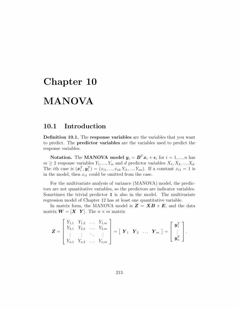
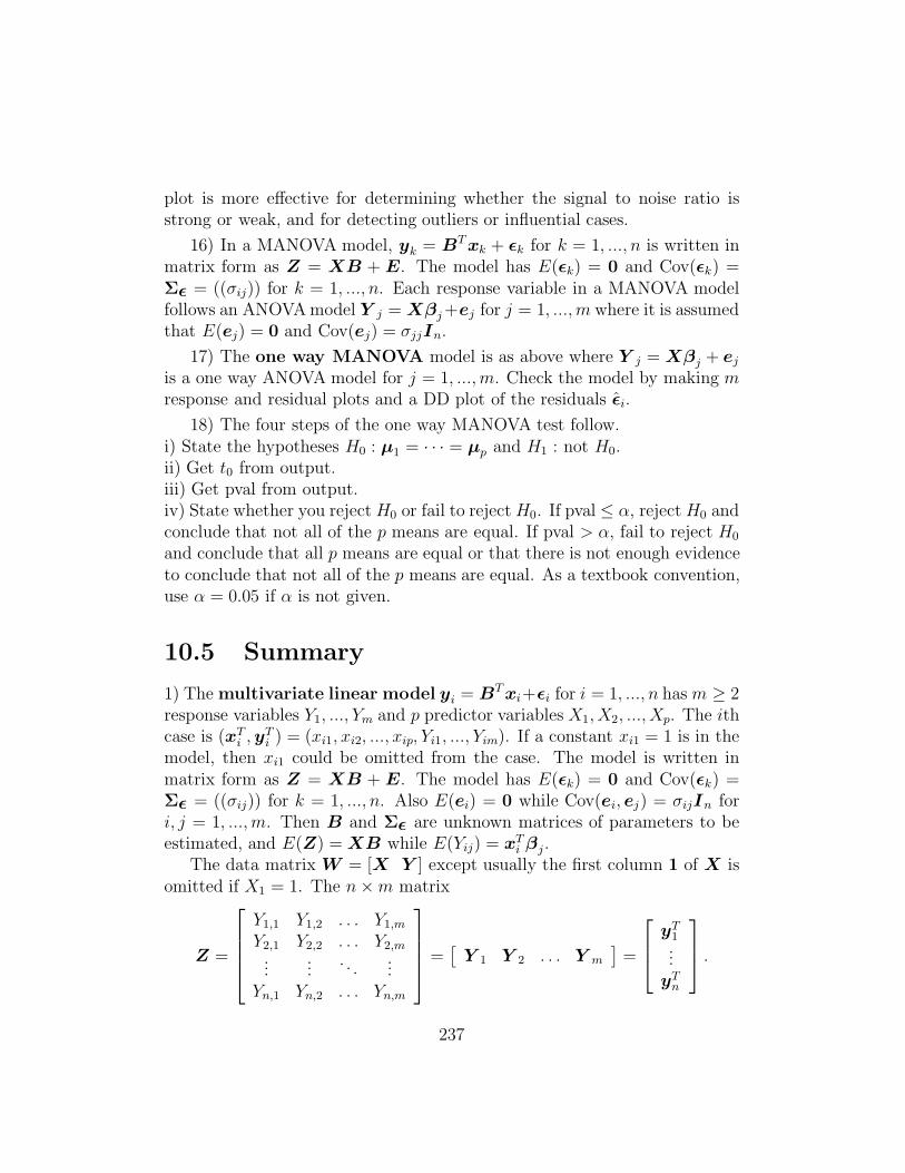
Chapter 10

MANOVA

10.1 Introduction

Definition 10.1. The response variables are the variables that you wantto predict. The predictor variables are the variables used to predict theresponse variables.

Notation. The MANOVA model yi = BT xi + εi for i = 1, ..., n hasm ≥ 2 response variables Y1, ..., Ym and d predictor variables X1, X2, ..., Xd.The ith case is (xT

i , yTi ) = (xi1, ..., xid, Yi1, ..., Yim). If a constant xi1 = 1 is

in the model, then xi1 could be omitted from the case.

For the multivariate analysis of variance (MANOVA) model, the predic-tors are not quantitative variables, so the predictors are indicator variables.Sometimes the trivial predictor 1 is also in the model. The multivariateregression model of Chapter 12 has at least one quantitative variable.

In matrix form, the MANOVA model is Z = XB + E, and the datamatrix W = [X Y ]. The n × m matrix

Z =

Y1,1 Y1,2 . . . Y1,m

Y2,1 Y2,2 . . . Y2,m

......

. . ....

Yn,1 Yn,2 . . . Yn,m

=[

Y 1 Y 2 . . . Y m

]

=

yT1...

yTn

.

213

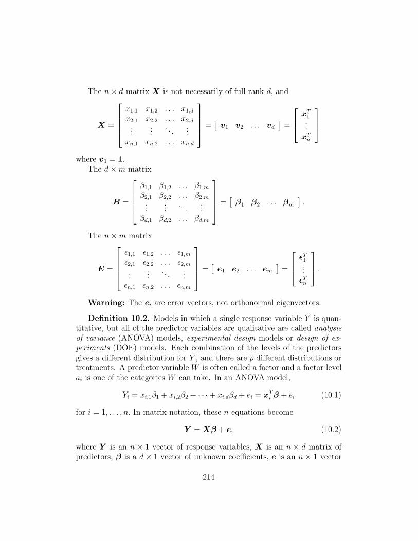
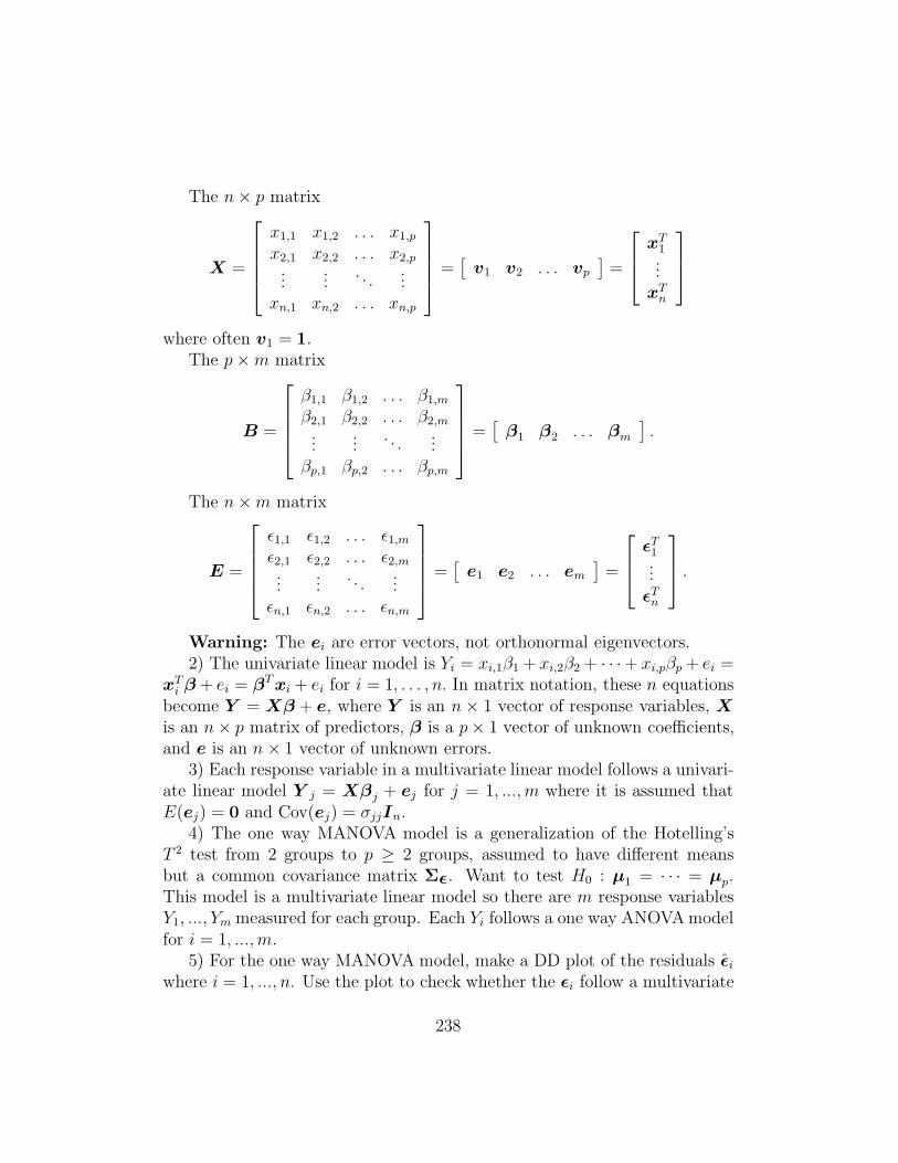
The n × d matrix X is not necessarily of full rank d, and

X =

x1,1 x1,2 . . . x1,d

x2,1 x2,2 . . . x2,d

......

. . ....

xn,1 xn,2 . . . xn,d

=[

v1 v2 . . . vd

]

=

xT1...

xTn

where v1 = 1.The d × m matrix

B =

β1,1 β1,2 . . . β1,m

β2,1 β2,2 . . . β2,m

......

. . ....

βd,1 βd,2 . . . βd,m

=[

β1 β2 . . . βm

]

.

The n × m matrix

E =

ε1,1 ε1,2 . . . ε1,m

ε2,1 ε2,2 . . . ε2,m

......

. . ....

εn,1 εn,2 . . . εn,m

=[

e1 e2 . . . em

]

=

εT1...

εTn

.

Warning: The ei are error vectors, not orthonormal eigenvectors.

Definition 10.2. Models in which a single response variable Y is quan-titative, but all of the predictor variables are qualitative are called analysisof variance (ANOVA) models, experimental design models or design of ex-periments (DOE) models. Each combination of the levels of the predictorsgives a different distribution for Y , and there are p different distributions ortreatments. A predictor variable W is often called a factor and a factor levelai is one of the categories W can take. In an ANOVA model,

Yi = xi,1β1 + xi,2β2 + · · · + xi,dβd + ei = xTi β + ei (10.1)

for i = 1, . . . , n. In matrix notation, these n equations become

Y = Xβ + e, (10.2)

where Y is an n × 1 vector of response variables, X is an n × d matrix ofpredictors, β is a d × 1 vector of unknown coefficients, e is an n × 1 vector

214

of unknown errors, and d ≥ p. Equivalently,

Y1

Y2...

Yn

=

x1,1 x1,2 . . . x1,d

x2,1 x2,2 . . . x2,d

......

. . ....

xn,1 xn,2 . . . xn,d

β1

β2...

βd

+

e1

e2...en

. (10.3)

The ei are iid with zero mean and variance σ2, and a linear model estimatorsuch as least squares is used to estimate the unknown parameters β and σ2.

Each response variable in a MANOVA model follows an ANOVA modelY j = Xβj + ej for j = 1, ..., m where it is assumed that E(ej) = 0 andCov(ej) = σjjIn. Hence the errors corresponding to the jth response areuncorrelated with variance σ2

j = σjj. Notice that the same design matrixX of predictors is used for each of the m models, but the jth responsevariable vector Y j, coefficient vector βj and error vector ej change and thusdepend on j. Hence for a one way MANOVA model, each response variablefollows a one way ANOVA model, while for a two way MANOVA model,each response variable follows a two way ANOVA model for j = 1, ..., m.

Once the ANOVA model is fixed, eg a one way ANOVA model, the designmatrix X depends on the parameterization of the ANOVA model. Thefitted values and residuals are the same for each parameterization, but theinterpretation of the parameters depend on the parameterization.

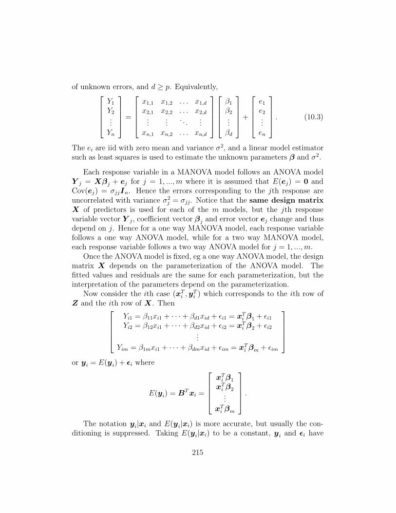
Now consider the ith case (xTi , yT

i ) which corresponds to the ith row ofZ and the ith row of X. Then

Yi1 = β11xi1 + · · · + βd1xid + εi1 = xTi β1 + εi1

Yi2 = β12xi1 + · · · + βd2xid + εi2 = xTi β2 + εi2

...Yim = β1mxi1 + · · · + βdmxid + εim = xT

i βm + εim

or yi = E(yi) + εi where

E(yi) = BT xi =

xTi β1

xTi β2...

xTi βm

.

The notation yi|xi and E(yi|xi) is more accurate, but usually the con-ditioning is suppressed. Taking E(yi|xi) to be a constant, yi and εi have

215

the same covariance matrix. In the MANOVA model, this covariance matrixΣε does not depend on i. Observations from different cases are uncorrelated(often independent), but the m errors for the m different response variablesfor the same case are correlated.

Definition 10.3. The MANOVA model yk = BTxk + εk for k =1, ..., n is written in matrix form as Z = XB + E. The model has E(εk) =0 and Cov(εk) = Σε = ((σij)) for k = 1, ..., n. Also E(ei) = 0 whileCov(ei, ej) = σijIn for i, j = 1, ..., m. Then B and Σε are unknown matricesof parameters to be estimated, and E(Z) = XB while E(Yij) = xT

i βj.Considering the kth row of Z, X and E shows that yT

k = xTk B + εT

k .

10.2 One Way ANOVA

Before describing the one way MANOVA model, it is useful to give a briefdescription on the one way ANOVA model.

Definition 10.4. A lurking variable is not one of the variables in thestudy, but may affect the relationships among the variables in the study.A unit is the experimental material assigned treatments, which are theconditions the investigator wants to study. The unit is experimental if it wasrandomly assigned to a treatment, and the unit is observational if it was notrandomly assigned to a treatment.

Definition 10.5. In an experiment, the investigators use randomiza-tion to assign treatments to units. To assign p treatments to n = n1+· · ·+np

experimental units, draw a random permutation of {1, ..., n}. Assign the firstn1 units treatment 1, the next n2 units treatment 2, ..., and the final np unitstreatment p.

Randomization allows one to do valid inference such as F tests of hypothe-ses and confidence intervals. Randomization also washes out the effects oflurking variables and makes the p treatment groups similar except for thetreatment. The effects of lurking variables are present in observational stud-ies defined in Definition 10.6.

Definition 10.6. In an observational study, investigators simply ob-serve the response, and the treatment groups need to be p random samples

216

from p populations (the levels) for valid inference.

Example 10.1. Consider using randomization to assign the followingnine people (units) to three treatment groups.

Carroll, Collin, Crawford, Halverson, Lawes,Stach, Wayman, Wenslow, Xumong

Balanced designs have the group sizes the same: ni ≡ h = n/p. Label theunits alphabetically so Carroll gets 1, ..., Xumong gets 9. The R/Splusfunction sample can be used to draw a random permutation. Then the first3 numbers in the permutation correspond to group 1, the next 3 to group 2and the final 3 to group 3. Using the output shown below, gives the following3 groups.

group 1: Stach, Wayman, Xumonggroup 2: Lawes, Carroll, Halversongroup 3: Collin, Wenslow, Crawford

> sample(9)

[1] 6 7 9 5 1 4 2 8 3

Often there is a table or computer file of units and related measurements,and it is desired to add the unit’s group to the end of the table. The mpackfunction rand reports a random permutation and the quantity groups[i] =treatment group for the ith person on the list. Since persons 6, 7 and 9 are ingroup 1, groups[7] = 1. Since Carroll is person 1 and is in group 2, groups[1]= 2, et cetera.

> rand(9,3)

$perm

[1] 6 7 9 5 1 4 2 8 3

$groups

[1] 2 3 3 2 2 1 1 3 1

Definition 10.7. Replication means that for each treatment, the ni

response variables Yi,1, ..., Yi,niare approximately iid random variables.

Example 10.2. a) If ten students work two types of paper mazes threetimes each, then there are 60 measurements that are not replicates. Each

217

student should work the six mazes in random order since speed increaseswith practice. For the ith student, let Zi1 be the average time to completethe three mazes of type 1, let Zi2 be the average time for mazes of type 2and let Di = Zi1 − Zi2. Then D1, ..., D10 are replicates.

b) Cobb (1998, p. 126) states that a student wanted to know if the shapesof sponge cells depends on the color (green or white). He measured hundredsof cells from one white sponge and hundreds of cells from one green sponge.There were only two units so n1 = 1 and n2 = 1. The student should haveused a sample of n1 green sponges and a sample of n2 white sponges to getmore replicates.

c) Replication depends on the goals of the study. Box, Hunter and Hunter(2005, p. 215-219) describes an experiment where the investigator times howlong it takes him to bike up a hill. Since the investigator is only interested inhis performance, each run up a hill is a replicate (the time for the ith run is asample from all possible runs up the hill by the investigator). If the interesthad been on the effect of eight treatment levels on student bicyclists, thenreplication would need n = n1 + · · · + n8 student volunteers where ni ridetheir bike up the hill under the conditions of treatment i.

Definition 10.8. Let fZ(z) be the pdf of Z. Then the family of pdfsfY (y) = fZ(y−µ) indexed by the location parameter µ, −∞ < µ < ∞, is thelocation family for the random variable Y = µ +Z with standard pdf fZ(z).

Definition 10.9. A one way fixed effects ANOVA model has a singlequalitative predictor variable W with p categories a1, ..., ap. There are pdifferent distributions for Y , one for each category ai. The distribution of

Y |(W = ai) ∼ fZ(y − µi)

where the location family has second moments. Hence all p distributionscome from the same location family with different location parameter µi andthe same variance σ2.

Definition 10.10. The one way fixed effects normal ANOVA model isthe special case where

Y |(W = ai) ∼ N(µi, σ2).

Example 10.3. The pooled 2 sample t–test is a special case of a oneway ANOVA model with p = 2. For example, one population could be ACT

218

scores for men and the second population ACT scores for women. Then W =gender and Y = score.

Notation. It is convenient to relabel the response variable Y1, ..., Yn asthe vector Y = (Y11, ..., Y1,n1

, Y21, ..., Y2,n2, ..., Yp1, ..., Yp,np)

T where the Yij areindependent and Yi1, ..., Yi,ni

are iid. Here j = 1, ..., ni where ni is the numberof cases from the ith level where i = 1, ..., p. Thus n1+· · ·+np = n. Similarlyuse double subscripts on the errors. Then there will be many equivalentparameterizations of the one way fixed effects ANOVA model.

Definition 10.11. The cell means model is the parameterization of theone way fixed effects ANOVA model such that

Yij = µi + eij

where Yij is the value of the response variable for the jth trial of the ithfactor level. The µi are the unknown means and E(Yij) = µi. The eij areiid from the location family with pdf fZ(z) and unknown variance σ2 =VAR(Yij) = VAR(eij). For the normal cell means model, the eij are iidN(0, σ2) for i = 1, ..., p and j = 1, ..., ni.

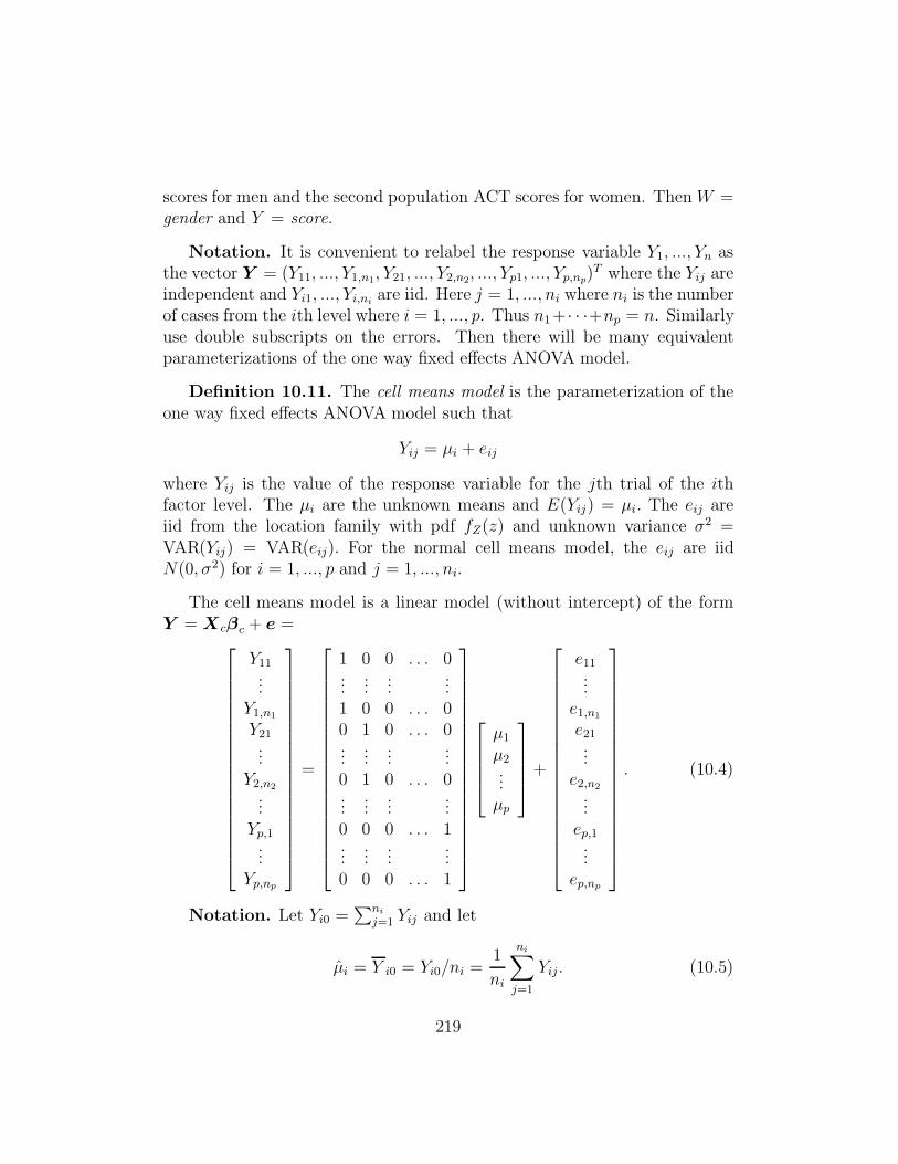
The cell means model is a linear model (without intercept) of the formY = Xcβc + e =

Y11...

Y1,n1

Y21...

Y2,n2

...Yp,1...

Yp,np

=

1 0 0 . . . 0...

......

...1 0 0 . . . 00 1 0 . . . 0...

......

...0 1 0 . . . 0...

......

...0 0 0 . . . 1...

......

...0 0 0 . . . 1

µ1

µ2...

µp

+

e11...

e1,n1

e21...

e2,n2

...ep,1...

ep,np

. (10.4)

Notation. Let Yi0 =∑ni

j=1 Yij and let

µi = Y i0 = Yi0/ni =1

ni

ni∑

j=1

Yij. (10.5)

219

Hence the “dot notation” means sum over the subscript corresponding to the0, eg j. Similarly, Y00 =

∑p

i=1

∑ni

j=1 Yij is the sum of all of the Yij.

Notice that the indicator variables used in the cell means model (10.4) arevh,k = 1 if the hth case has W = ak, and vhk

= 0, otherwise, for k = 1, ..., pand h = 1, ..., n. So Yij has vh,k = 1 only if i = k and j = 1, ..., ni. Here vk isthe kth column of Xc. The model can use p indicator variables for the factorinstead of p − 1 indicator variables because the model does not contain anintercept. Also notice that

E(Y ) = Xcβc = (µ1, ..., µ1, µ2, ..., µ2, ..., µp, ..., µp)T ,

(XTc Xc) = diag(n1, ..., np) and XT

c Y = (Y10, ..., Y10, Y20, ..., Y20, ..., Yp0, ..., Yp0)T .

Hence (XTc Xc)

−1 = diag(1/n1, ..., 1/np) and the OLS estimator

βc = (XTc Xc)

−1XTc Y = (Y 10, ..., Y p0)

T = (µ1, ..., µp)T .

Thus Y = Xcβc = (Y 10, ..., Y 10, ..., Y p0, ..., Y p0)T . Hence the ijth fitted value

isYij = Y i0 = µi (10.6)

and the ijth residual is

rij = Yij − Yij = Yij − µi. (10.7)

Since the cell means model is a linear model, there is an associated re-sponse plot and residual plot. However, many of the interpretations of theOLS quantities for ANOVA models differ from the interpretations for multi-ple linear regression (MLR) models. First, for MLR models, the conditionaldistribution Y |x makes sense even if x is not one of the observed xi providedthat x is not far from the xi. This fact makes MLR very powerful. For MLR,at least one of the variables in x is a continuous predictor. For the one wayfixed effects ANOVA model, the p distributions Y |xi make sense where xT

i

is a row of Xc.Also, the OLS MLR ANOVA F test for the cell means model tests H0 :

β = 0 ≡ H0 : µ1 = · · · = µp = 0, while the one way fixed effects ANOVA Ftest given after Definition 10.15 tests H0 : µ1 = · · · = µp.

Definition 10.12. Consider the one way fixed effects ANOVA model.The response plot is a plot of Yij ≡ µi versus Yij and the residual plot is a

220

plot of Yij ≡ µi versus rij . Add the identity line to the response plot andr = 0 line to the residual plot as visual aids.

The points in the response plot scatter about the identity line and thepoints in the residual plot scatter about the r = 0 line, but the scatter neednot be in an evenly populated band. A dot plot of Z1, ..., Zm consists of anaxis and m points each corresponding to the value of Zi. The response plotconsists of p dot plots, one for each value of µi. The dot plot correspondingto µi is the dot plot of Yi1, ..., Yi,ni

. The p dot plots should have roughly thesame amount of spread, and each µi corresponds to level ai. If a new levelaf corresponding to xf was of interest, hopefully the points in the responseplot corresponding to af would form a dot plot at µf similar in spread tothe other dot plots, but it may not be possible to predict the value of µf .Similarly, the residual plot consists of p dot plots, and the plot correspondingto µi is the dot plot of ri1, ..., ri,ni

.Assume that each ni ≥ 10. Under the assumption that the Yij are from

the same location scale family with different parameters µi, each of the pdot plots should have roughly the same shape and spread. This assumptionis easier to judge with the residual plot. If the response plot looks like theresidual plot, then a horizontal line fits the p dot plots about as well as theidentity line, and there is not much difference in the µi. If the identity line isclearly superior to any horizontal line, then at least some of the means differ.

Definition 10.13. An outlier corresponds to a case that is far from thebulk of the data. Look for a large vertical distance of the plotted point fromthe identity line or the r = 0 line.

Rule of thumb 10.1. Mentally add 2 lines parallel to the identity lineand 2 lines parallel to the r = 0 line that cover most of the cases. Then acase is an outlier if it is well beyond these 2 lines.

This rule often fails for large outliers since often the identity line goesthrough or near a large outlier so its residual is near zero. A response that isfar from the bulk of the data in the response plot is a “large outlier” (largein magnitude). Look for a large gap between the bulk of the data and thelarge outlier.

Suppose there is a dot plot of nj cases corresponding to level aj that isfar from the bulk of the data. This dot plot is probably not a cluster of “badoutliers” if nj ≥ 4 and n ≤ 50. If nj = 1, such a case may be a large outlier.

221

Rule of thumb 10.2. Often an outlier is very good, but more often anoutlier is due to a measurement error and is very bad.

The assumption of the Yij coming from the same location scale familywith different location parameters µi and the same constant variance σ2

is a big assumption and often does not hold. Another way to check thisassumption is to make a box plot of the Yij for each i. The box in the boxplot corresponds to the lower, middle and upper quartiles of the Yij . Themiddle quartile is just the sample median of the data mij: at least half of theYij ≥ mij and at least half of the Yij ≤ mij. The p boxes should be roughlythe same length and the median should occur in roughly the same position(eg in the center) of each box. The “whiskers” in each plot should also beroughly similar. Histograms for each of the p samples could also be made.All of the histograms should look similar in shape.

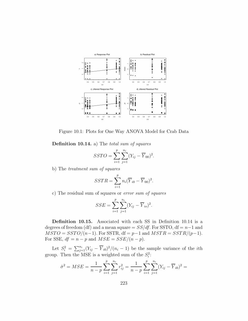
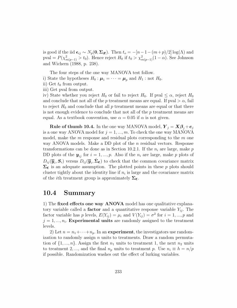
Example 10.4. Kuehl (1994, p. 128) gives data for counts of hermitcrabs on 25 different transects in each of six different coastline habitats. LetZ be the count. Then the response variable Y = log10(Z+1/6). Although thecounts Z varied greatly, each habitat had several counts of 0 and often therewere several counts of 1, 2 or 3. Hence Y is not a continuous variable. Thecell means model was fit with ni = 25 for i = 1, ..., 6. Each of the six habitatswas a level. Figure 10.1a and b shows the response plot and residual plot.There are 6 dot plots in each plot. Because several of the smallest values ineach plot are identical, it does not always look like the identity line is passingthrough the six sample means Y i0 for i = 1, ..., 6. In particular, examine thedot plot for the smallest mean (look at the 25 dots furthest to the left thatfall on the vertical line FIT ≈ 0.36). Random noise (jitter) has been added tothe response and residuals in Figure 10.1c and d. Now it is easier to comparethe six dot plots. They seem to have roughly the same spread.

The plots contain a great deal of information. The response plot canbe used to explain the model, check that the sample from each population(treatment) has roughly the same shape and spread, and to see which pop-ulations have similar means. Since the response plot closely resembles theresidual plot in Figure 10.1, there may not be much difference in the sixpopulations. Linearity seems reasonable since the samples scatter about theidentity line. The residual plot makes the comparison of “similar shape” and“spread” easier.

222

FIT

Y

0.4 0.5 0.6 0.7 0.8 0.9 1.00

12

a) Response Plot

FIT

RE

SID

0.4 0.5 0.6 0.7 0.8 0.9 1.0

-10

1

b) Residual Plot

FIT

JY

0.4 0.5 0.6 0.7 0.8 0.9 1.0

01

2

c) Jittered Response Plot

FIT

JR

0.4 0.5 0.6 0.7 0.8 0.9 1.0

-10

1

d) Jittered Residual Plot

Figure 10.1: Plots for One Way ANOVA Model for Crab Data

Definition 10.14. a) The total sum of squares

SSTO =

p∑

i=1

ni∑

j=1

(Yij − Y 00)2.

b) The treatment sum of squares

SSTR =

p∑

i=1

ni(Y i0 − Y 00)2.

c) The residual sum of squares or error sum of squares

SSE =

p∑

i=1

ni∑

j=1

(Yij − Y io)2.

Definition 10.15. Associated with each SS in Definition 10.14 is adegrees of freedom (df) and a mean square = SS/df. For SSTO, df = n−1 andMSTO = SSTO/(n−1). For SSTR, df = p−1 and MSTR = SSTR/(p−1).For SSE, df = n − p and MSE = SSE/(n − p).

Let S2i =

∑ni

j=1(Yij − Y i0)2/(ni − 1) be the sample variance of the ith

group. Then the MSE is a weighted sum of the S2i :

σ2 = MSE =1

n − p

p∑

i=1

ni∑

j=1

r2ij =

1

n − p

p∑

i=1

ni∑

j=1

(Yij − Y i0)2 =

223

1

n − p

p∑

i=1

(ni − 1)S2i = S2

pool

where S2pool is known as the pooled variance estimator.

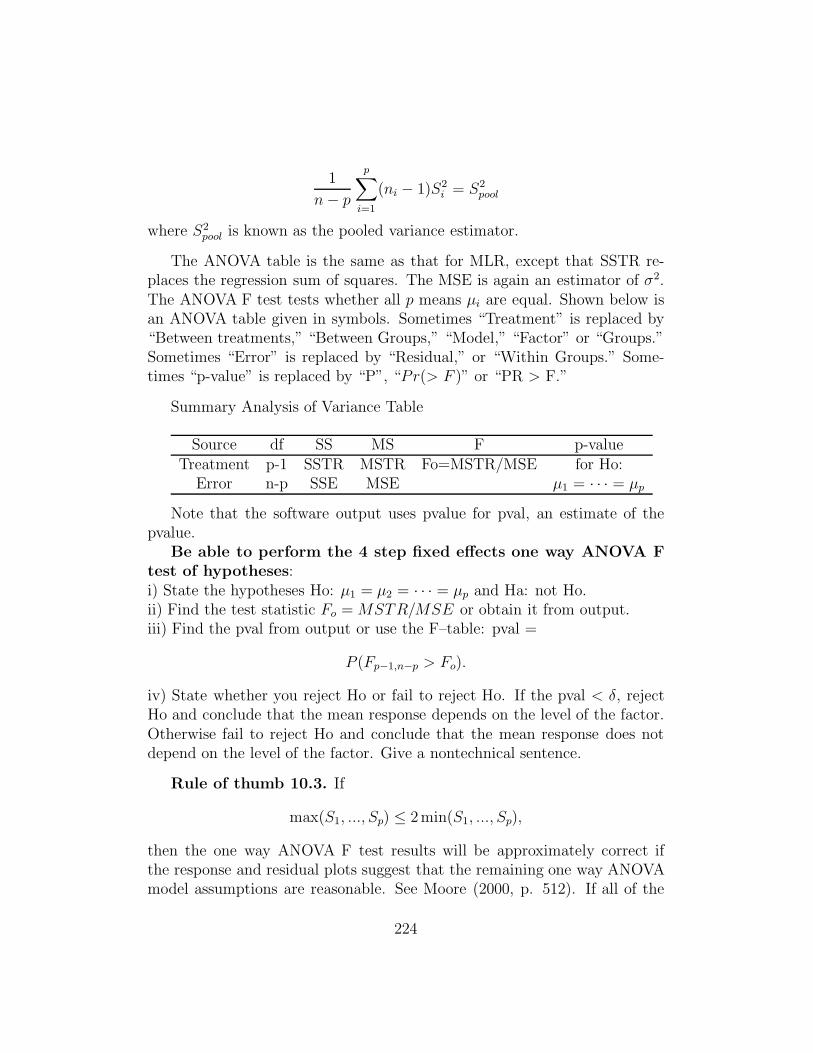
The ANOVA table is the same as that for MLR, except that SSTR re-places the regression sum of squares. The MSE is again an estimator of σ2.The ANOVA F test tests whether all p means µi are equal. Shown below isan ANOVA table given in symbols. Sometimes “Treatment” is replaced by“Between treatments,” “Between Groups,” “Model,” “Factor” or “Groups.”Sometimes “Error” is replaced by “Residual,” or “Within Groups.” Some-times “p-value” is replaced by “P”, “Pr(> F )” or “PR > F.”

Summary Analysis of Variance Table

Source df SS MS F p-valueTreatment p-1 SSTR MSTR Fo=MSTR/MSE for Ho:

Error n-p SSE MSE µ1 = · · · = µp

Note that the software output uses pvalue for pval, an estimate of thepvalue.

Be able to perform the 4 step fixed effects one way ANOVA Ftest of hypotheses:i) State the hypotheses Ho: µ1 = µ2 = · · · = µp and Ha: not Ho.ii) Find the test statistic Fo = MSTR/MSE or obtain it from output.iii) Find the pval from output or use the F–table: pval =

P (Fp−1,n−p > Fo).

iv) State whether you reject Ho or fail to reject Ho. If the pval < δ, rejectHo and conclude that the mean response depends on the level of the factor.Otherwise fail to reject Ho and conclude that the mean response does notdepend on the level of the factor. Give a nontechnical sentence.

Rule of thumb 10.3. If

max(S1, ..., Sp) ≤ 2min(S1, ..., Sp),

then the one way ANOVA F test results will be approximately correct ifthe response and residual plots suggest that the remaining one way ANOVAmodel assumptions are reasonable. See Moore (2000, p. 512). If all of the

224

ni ≥ 5, replace the standard deviations by the ranges of the dot plots whenexamining the response and residual plots.

Remark 10.1. If the units are a representative sample of some popula-tion of interest, then randomization of units into groups makes the assump-tion that Yi1, ..., Yi,ni

are iid hold to a useful approximation for large sampletheory. Random sampling from populations also induces the iid assump-tion. Linearity can be checked with the response plot, and similar shape andspread of the location families can be checked with both the response andresidual plots. Also check that outliers are not present. If the p dot plots inthe response plot are approximately symmetric, then the sample sizes ni canbe smaller than if the dot plots are skewed.

Remark 10.2. When the assumption that the p groups come from thesame location family with finite variance σ2 is violated, the one way ANOVAF test may not make much sense because unequal means may not imply thesuperiority of one category over another. Suppose Y is the time in minutesuntil relief from a headache and that Y1j ∼ N(60, 1) while Y2j ∼ N(65, σ2).If σ2 = 1, then the type 1 medicine gives headache relief 5 minutes faster, onaverage, and is superior, all other things being equal. But if σ2 = 100, thenmany patients taking medicine 2 experience much faster pain relief than thosetaking medicine 1, and many experience much longer time until pain relief.In this situation, predictor variables that would identify which medicine isfaster for a given patient would be very useful.

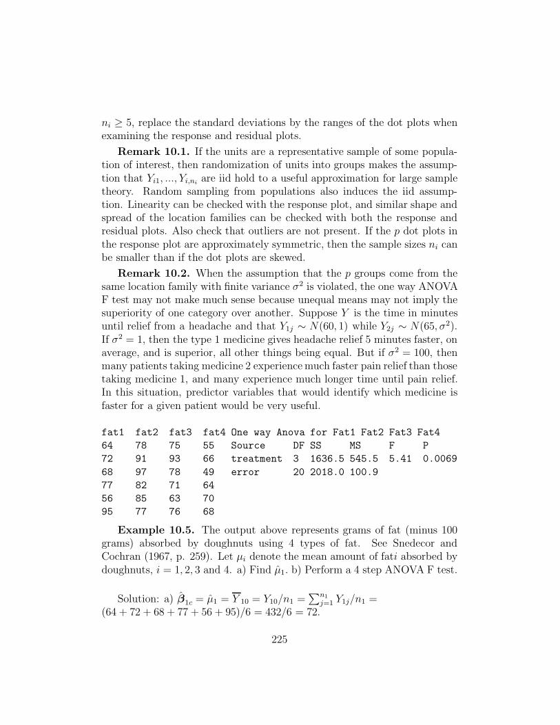
fat1 fat2 fat3 fat4 One way Anova for Fat1 Fat2 Fat3 Fat4

64 78 75 55 Source DF SS MS F P

72 91 93 66 treatment 3 1636.5 545.5 5.41 0.0069

68 97 78 49 error 20 2018.0 100.9

77 82 71 64

56 85 63 70

95 77 76 68

Example 10.5. The output above represents grams of fat (minus 100grams) absorbed by doughnuts using 4 types of fat. See Snedecor andCochran (1967, p. 259). Let µi denote the mean amount of fati absorbed bydoughnuts, i = 1, 2, 3 and 4. a) Find µ1. b) Perform a 4 step ANOVA F test.

Solution: a) β1c = µ1 = Y 10 = Y10/n1 =∑n1

j=1 Y1j/n1 =(64 + 72 + 68 + 77 + 56 + 95)/6 = 432/6 = 72.

225

b) i) H0 : µ1 = µ2 = µ3 = µ4 Ha: not H0

ii) F = 5.41iii) pval = 0.0069iv) Reject H0, the mean amount of fat absorbed by doughnuts depends

on the type of fat.

Definition 10.16. A contrast C =∑p

i=1 kiµi where∑p

i=1 ki = 0. The

estimated contrast is C =∑p

i=1 kiY i0.

If the null hypothesis of the fixed effects one way ANOVA test is nottrue, then not all of the means µi are equal. Researchers will often havehypotheses, before examining the data, that they desire to test. Often sucha hypothesis can be put in the form of a contrast. For example, the contrastC = µi−µj is used to compare the means of the ith and jth groups while thecontrast µ1 − (µ2 + · · ·+µp)/(p− 1) is used to compare the last p− 1 groupswith the 1st group. This contrast is useful when the 1st group correspondsto a standard or control treatment while the remaining groups correspond tonew treatments.

Assume that the normal cell means model is a useful approximation tothe data. Then the Y i0 ∼ N(µi, σ

2/ni) are independent, and

C =

p∑

i=1

kiY i0 ∼ N

(

C, σ2

p∑

i=1

k2i

ni

)

.

Hence the standard error

SE(C) =

√

√

√

√MSE

p∑

i=1

k2i

ni

.

The degrees of freedom is equal to the MSE degrees of freedom = n − p.Consider a family of null hypotheses for contrasts {Ho :

∑p

i=1 kiµi = 0where

∑pi=1 ki = 0 and the ki may satisfy other constraints}. Let δS denote

the probability of a type I error for a single test from the family where a typeI error is a false rejection. The family level δF is an upper bound on the(usually unknown) size δT . Know how to interpret δF ≈ δT =P(of making at least one type I error among the family of contrasts).

Two important families of contrasts are the family of all possible con-trasts and the family of pairwise differences Cij = µi − µj where i 6= j. The

226

Scheffe multiple comparisons procedure has a δF for the family of all possiblecontrasts while the Tukey multiple comparisons procedure has a δF for thefamily of all

(

p

2

)

pairwise contrasts.To interpret output for multiple comparisons procedures, the underlined

means or blocks of letters besides groups of means indicate that the groupof means are not significantly different.

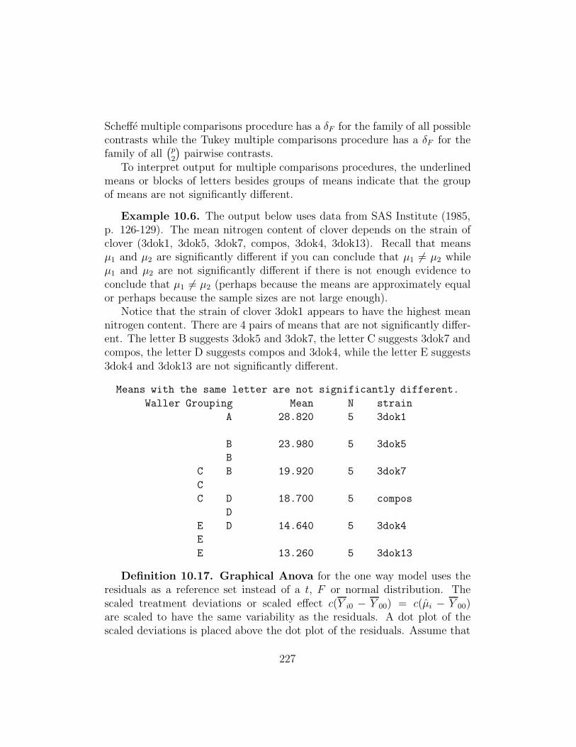
Example 10.6. The output below uses data from SAS Institute (1985,p. 126-129). The mean nitrogen content of clover depends on the strain ofclover (3dok1, 3dok5, 3dok7, compos, 3dok4, 3dok13). Recall that meansµ1 and µ2 are significantly different if you can conclude that µ1 6= µ2 whileµ1 and µ2 are not significantly different if there is not enough evidence toconclude that µ1 6= µ2 (perhaps because the means are approximately equalor perhaps because the sample sizes are not large enough).

Notice that the strain of clover 3dok1 appears to have the highest meannitrogen content. There are 4 pairs of means that are not significantly differ-ent. The letter B suggests 3dok5 and 3dok7, the letter C suggests 3dok7 andcompos, the letter D suggests compos and 3dok4, while the letter E suggests3dok4 and 3dok13 are not significantly different.

Means with the same letter are not significantly different.

Waller Grouping Mean N strain

A 28.820 5 3dok1

B 23.980 5 3dok5

B

C B 19.920 5 3dok7

C

C D 18.700 5 compos

D

E D 14.640 5 3dok4

E

E 13.260 5 3dok13

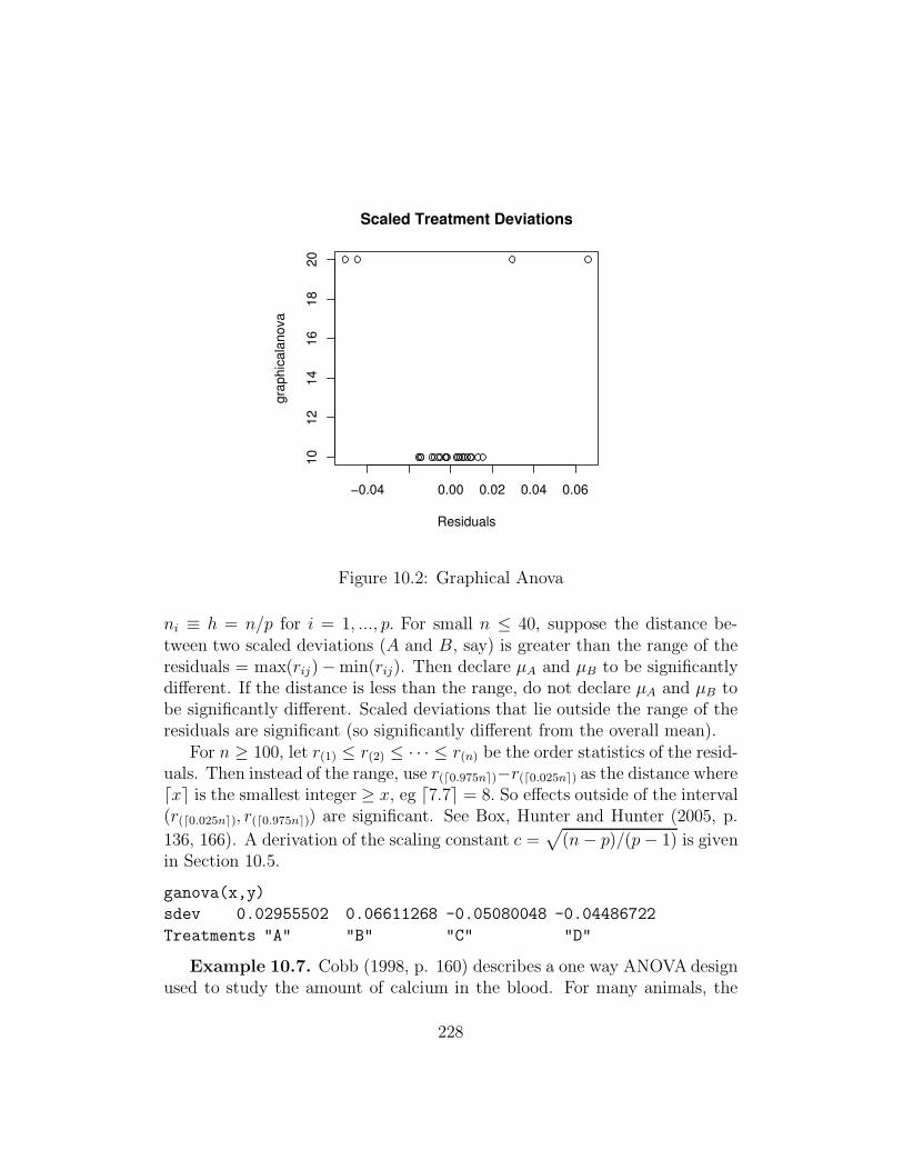
Definition 10.17. Graphical Anova for the one way model uses theresiduals as a reference set instead of a t, F or normal distribution. Thescaled treatment deviations or scaled effect c(Y i0 − Y 00) = c(µi − Y 00)are scaled to have the same variability as the residuals. A dot plot of thescaled deviations is placed above the dot plot of the residuals. Assume that

227

−0.04 0.00 0.02 0.04 0.06

10

12

14

16

18

20

Residuals

gra

ph

ica

lan

ova

Scaled Treatment Deviations

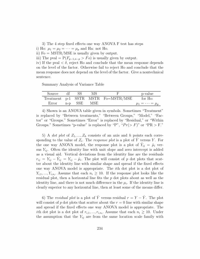
Figure 10.2: Graphical Anova

ni ≡ h = n/p for i = 1, ..., p. For small n ≤ 40, suppose the distance be-tween two scaled deviations (A and B, say) is greater than the range of theresiduals = max(rij)−min(rij). Then declare µA and µB to be significantlydifferent. If the distance is less than the range, do not declare µA and µB tobe significantly different. Scaled deviations that lie outside the range of theresiduals are significant (so significantly different from the overall mean).

For n ≥ 100, let r(1) ≤ r(2) ≤ · · · ≤ r(n) be the order statistics of the resid-uals. Then instead of the range, use r(d0.975ne)−r(d0.025ne) as the distance wheredxe is the smallest integer ≥ x, eg d7.7e = 8. So effects outside of the interval(r(d0.025ne), r(d0.975ne)) are significant. See Box, Hunter and Hunter (2005, p.

136, 166). A derivation of the scaling constant c =√

(n − p)/(p − 1) is givenin Section 10.5.

ganova(x,y)

sdev 0.02955502 0.06611268 -0.05080048 -0.04486722

Treatments "A" "B" "C" "D"

Example 10.7. Cobb (1998, p. 160) describes a one way ANOVA designused to study the amount of calcium in the blood. For many animals, the

228

body’s ability to use calcium depends on the level of certain hormones inthe blood. The response was 1/(level of plasma calcium). The four groupswere A: Female controls, B: Male controls, C: Females given hormone and D:Males given hormone. There were 10 birds of each gender, and five from eachgender were given the hormone. The output above uses the mpack functionganova to produce Figure 10.2.

In Figure 10.2, the top dot plot has the scaled treatment deviations. Fromleft to right, these correspond to C, D, A and B since the output shows thatthe deviation corresponding to C is the smallest with value −0.050. Since thedeviations corresponding to C and D are much closer than the range of theresiduals, the C and D effects yielded similar mean response values. A andB appear to be significantly different from C and D. The distance betweenthe scaled A and B treatment deviations is about the same as the distancebetween the smallest and largest residuals, so there is only marginal evidencethat the A and B effects are significantly different.

Since all 4 scaled deviations lie outside of the range of the residuals, alleffects A, B, C and D appear to be significant.

10.2.1 Response Transformations for ANOVA Models

A model for an experimental design is Yi = E(Yi) + ei for i = 1, ..., n wherethe error ei = Yi − E(Yi) and E(Yi) ≡ E(Yi|xi) is the expected value of theresponse Yi for a given vector of predictors xi. Many models can be fit withleast squares (OLS or LS) and are linear models of the form

Yi = xi,1β1 + xi,2β2 + · · · + xi,pβp + ei = xTi β + ei

for i = 1, . . . , n. Often xi,1 ≡ 1 for all i. In matrix notation, these n equationsbecome

Y = Xβ + e,

where Y is an n × 1 vector of dependent variables, X is an n × p designmatrix of predictors, β is a p × 1 vector of unknown coefficients, and e isan n × 1 vector of unknown errors. If the fitted values are Yi = xT

i β, thenYi = Yi + ri where the residuals ri = Yi − Yi.

The applicability of an experimental design model can be expanded byallowing response transformations. An important class of response transfor-mation models adds an additional unknown transformation parameter λo,

229

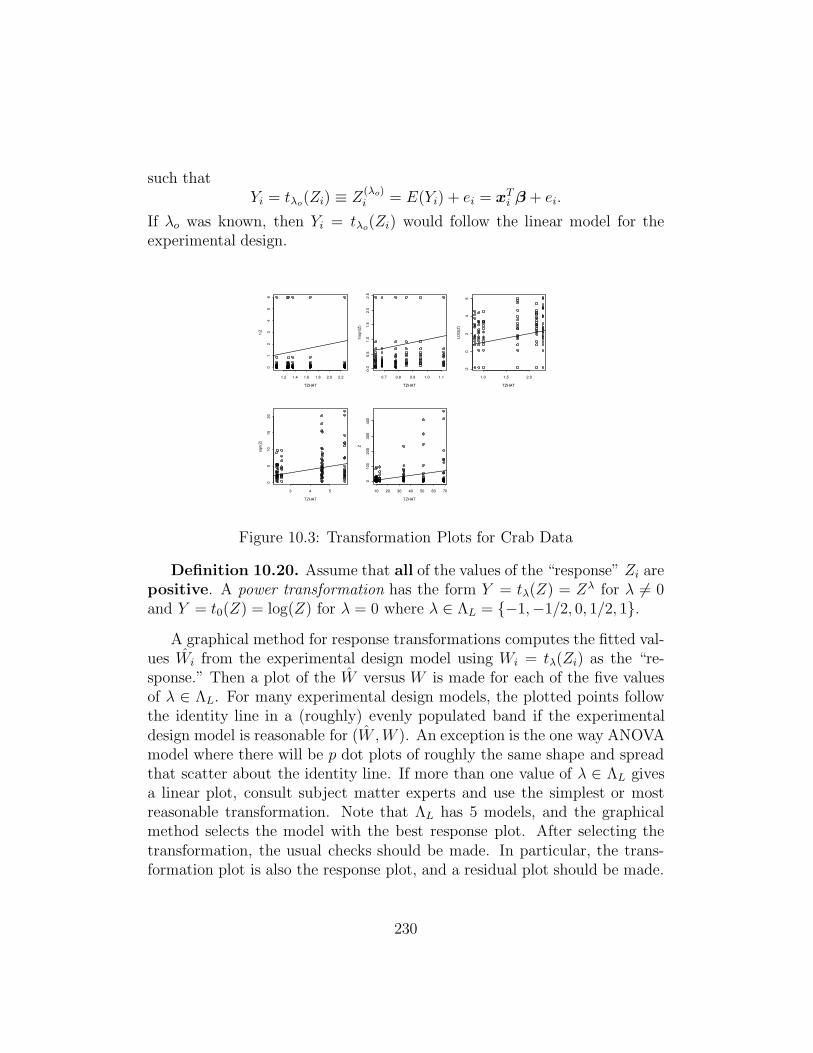
such thatYi = tλo(Zi) ≡ Z

(λo)i = E(Yi) + ei = xT

i β + ei.

If λo was known, then Yi = tλo(Zi) would follow the linear model for theexperimental design.

TZHAT

1/Z

1.2 1.4 1.6 1.8 2.0 2.2

01

23

45

6

TZHAT

1/s

qrt

(Z)

0.7 0.8 0.9 1.0 1.1

0.0

0.5

1.0

1.5

2.0

2.5

TZHAT

LO

G(Z

)

1.0 1.5 2.0

-20

24

6

TZHAT

sqrt

(Z)

3 4 5

05

10

15

20

TZHAT

Z

10 20 30 40 50 60 70

0100

200

300

400

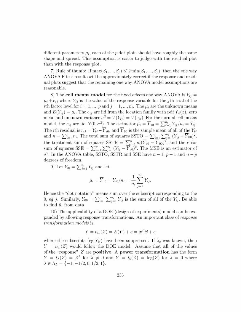
Figure 10.3: Transformation Plots for Crab Data

Definition 10.20. Assume that all of the values of the “response” Zi arepositive. A power transformation has the form Y = tλ(Z) = Zλ for λ 6= 0and Y = t0(Z) = log(Z) for λ = 0 where λ ∈ ΛL = {−1,−1/2, 0, 1/2, 1}.

A graphical method for response transformations computes the fitted val-ues Wi from the experimental design model using Wi = tλ(Zi) as the “re-sponse.” Then a plot of the W versus W is made for each of the five valuesof λ ∈ ΛL. For many experimental design models, the plotted points followthe identity line in a (roughly) evenly populated band if the experimentaldesign model is reasonable for (W , W ). An exception is the one way ANOVAmodel where there will be p dot plots of roughly the same shape and spreadthat scatter about the identity line. If more than one value of λ ∈ ΛL givesa linear plot, consult subject matter experts and use the simplest or mostreasonable transformation. Note that ΛL has 5 models, and the graphicalmethod selects the model with the best response plot. After selecting thetransformation, the usual checks should be made. In particular, the trans-formation plot is also the response plot, and a residual plot should be made.

230

Definition 10.21. A transformation plot is a plot of (W , W ) with theidentity line added as a visual aid.

In the following example, the plots show tλ(Z) on the vertical axis. Thelabel “TZHAT” of the horizontal axis are the fitted values that result fromusing tλ(Z) as the “response” in the software.

For one way ANOVA models with ni ≡ m ≥ 5, look for a transformationplot that satisfies the following conditions. i) The p dot plots scatter aboutthe identity line with similar shape and spread. ii) Dot plots with more skeware worse than dot plots with less skew or dot plots that are approximatelysymmetric. iii) Spread that increases or decreases with TZHAT is bad.

Example 10.4, continued. Following Kuehl (1994, p. 128), let C bethe count of crabs and let the “response” Z = C + 1/6. Figure 10.3 showsthe five transformation plots. The transformation log(Z) results in dot plotsthat have roughly the same shape and spread. The transformations 1/Z and1/√

Z do not handle the 0 counts well, and the dot plots fail to cover theidentity line. The transformations

√Z and Z have variance that increases

with the mean.

Remark 10.4. The graphical method for response transformations canbe used for design models that are linear models, not just one way ANOVAmodels. The method is nearly identical to that of Chapter 12, but ΛL only has

5 values. The log rule states that if all of the Zi > 0 and ifmax(Zi)

min(Zi)≥ 10,

then the response transformation Y = log(Z) will often work.

10.3 One Way MANOVA

Using double subscripts will be useful for describing the one way MANOVAmodel. Suppose there independent random samples from p different pop-ulations (treatments), or n =

∑p

i=1 ni and ni cases are randomly assignedto p treatment groups. Then the group sample sizes are ni for i = 1, ..., p.Assume that m response variables yij = (Yij1, ..., Yijm)T are measured forthe ith treatment. Hence i = 1, ..., p and j = 1, ..., ni. The Yijk follow dif-ferent one way ANOVA models for k = 1, ..., m. Assume E(yij) = µi andCov(yij) = Σε. Hence the p treatments have different mean vectors µi, butcommon covariance matrix Σε. (This assumption can be relaxed for p = 2

231

with the appropriate 2 sample Hotelling’s T 2 test.)The one way MANOVA is used to test H0 : µ1 = µ2 = · · · = µp. Often

µi = µ + τ i, so H0 becomes H0 : τ 1 = · · · = τ p. If m = 1, the oneway MANOVA model is the one way ANOVA model. MANOVA is usefulsince it takes into account the correlations between the m response variables.Performing m ANOVA tests fails to account for these correlations, but can bea useful diagnostic. The Hotelling’s T 2 test that uses a common covariancematrix is a special case of the one way MANOVA model with m = 2.

Let µi = µ + τ i where∑p

i=1 niτ i = 0. The jth case from the ith pop-ulation or treatment group is yij = µ + τ j + eij where eij is an errorvector, i = 1, ..., p and j = 1, ..., ni. Let y = µ =

∑pi=1

∑ni

j=1 yij/n bethe overall mean. Let yi =

∑ni

j=1 yij/ni so τ i = yi − y. Let the residualεij = yij−yi = yij−µ−τ i. Then yij = y+(yi−y)+(yij−yi) = µ+τ i+εij.

Let Si be the sample covariance matrix corresponding to the ith treat-ment group. Then the within sum of squares and cross products matrixis W = (n1 − 1)S1 + · · · + (np − 1)Sp =

∑pi=1

∑ni

j=1(yij − yi)(yij − yi)T .

Then Σε = W /(n− p). The treatment or between sum of squares and crossproducts matrix is B =

∑p

i=1 ni(yi − y)(yi − y)T . The total corrected (forthe mean) sum of squares and cross products matrix is T = B + W =∑p

i=1

∑ni

j=1(yij − y)(yij − y)T . Note that T /(n − 1) is the usual sample co-variance matrix if it is assumed that all n of the yij are iid so that the µi ≡ µ

for i = 1, ..., p.The one way MANOVA model is yij = µ + τ i + εij where the εij are iid

with E(εij) = 0 and Cov(εij) = Σε. The MANOVA table is shown below.

Summary One Way MANOVA Table

Source matrix dfTreatment or Between B p − 1

Residual or Error or Within W n − pTotal (corrected) T n − 1

If all n of the yij are iid with E(yij) = µ and Cov(yij) = Σε, it can be

shown that A/dfP→ Σε where A = W , B or T and df is the corresponding

degrees of freedom. Let t0 be the test statistic. Although Pillai’s trace isrobust to nonnormality, often Wilk’s lambda is used. Wilk’s lambda

Λ =|W |

|B + W | =|W ||T |

232

is good if the iid εij ∼ Np(0,Σx). Then to = −[n−1− (m+p)/2] log(Λ) andpval = P (χ2

m(p−1) > t0). Hence reject H0 if t0 > χ2m(p−1)(1− α). See Johnson

and Wichern (1988, p. 238).

The four steps of the one way MANOVA test follow.i) State the hypotheses H0 : µ1 = · · · = µp and H1 : not H0.ii) Get t0 from output.iii) Get pval from output.iv) State whether you reject H0 or fail to reject H0. If pval ≤ α, reject H0

and conclude that not all of the p treatment means are equal. If pval > α, failto reject H0 and conclude that all p treatment means are equal or that thereis not enough evidence to conclude that not all of the p treatment means areequal. As a textbook convention, use α = 0.05 if α is not given.

Rule of thumb 10.4. In the one way MANOVA model, Y j = Xβj +ej

is a one way ANOVA model for j = 1, ..., m. To check the one way MANOVAmodel, make the m response and residual plots corresponding to the m oneway ANOVA models. Make a DD plot of the n residual vectors. Responsetransformations can be done as in Section 10.2.1. If the ni are large, make pDD plots of the yij for i = 1, ..., p. Also if the ni are large, make p plots of

Dij(yi, Si) versus Dij(yi, Σε) to check that the common covariance matrixΣε is an adequate assumption. The plotted points in these p plots shouldcluster tightly about the identity line if ni is large and the covariance matrixof the ith treatment group is approximately Σε.

10.4 Summary

1) The fixed effects one way ANOVA model has one qualitative explana-tory variable called a factor and a quantitative response variable Yij . Thefactor variable has p levels, E(Yij) = µi and V (Yij) = σ2 for i = 1, ..., p andj = 1, ..., ni. Experimental units are randomly assigned to the treatmentlevels.

2) Let n = n1+· · ·+np. In an experiment, the investigators use random-ization to randomly assign n units to treatments. Draw a random permuta-tion of {1, ..., n}. Assign the first n1 units to treatment 1, the next n2 unitsto treatment 2, ..., and the final np units to treatment p. Use ni ≡ h = n/pif possible. Randomization washes out the effect of lurking variables.

233

3) The 4 step fixed effects one way ANOVA F test has stepsi) Ho: µ1 = µ2 = · · · = µp and Ha: not Ho.ii) Fo = MSTR/MSE is usually given by output.iii) The pval = P(Fp−1,n−p > Fo) is usually given by output.iv) If the pval < δ, reject Ho and conclude that the mean response dependson the level of the factor. Otherwise fail to reject Ho and conclude that themean response does not depend on the level of the factor. Give a nontechnicalsentence.

Summary Analysis of Variance Table

Source df SS MS F p-valueTreatment p-1 SSTR MSTR Fo=MSTR/MSE for Ho:

Error n-p SSE MSE µ1 = · · · = µp

4) Shown is an ANOVA table given in symbols. Sometimes “Treatment”is replaced by “Between treatments,” “Between Groups,” “Model,” “Fac-tor” or “Groups.” Sometimes “Error” is replaced by “Residual,” or “WithinGroups.” Sometimes “p-value” is replaced by “P”, “Pr(> F )” or “PR > F.”

5) A dot plot of Z1, ..., Zh consists of an axis and h points each corre-sponding to the value of Zi. The response plot is a plot of Y versus Y . Forthe one way ANOVA model, the response plot is a plot of Yij = µi ver-sus Yij . Often the identity line with unit slope and zero intercept is addedas a visual aid. Vertical deviations from the identity line are the residualsrij = Yij − Yij = Yij − µi. The plot will consist of p dot plots that scat-ter about the identity line with similar shape and spread if the fixed effectsone way ANOVA model is appropriate. The ith dot plot is a dot plot ofYi,1, ..., Yi,ni

. Assume that each ni ≥ 10. If the response plot looks like theresidual plot, then a horizontal line fits the p dot plots about as well as theidentity line, and there is not much difference in the µi. If the identity line isclearly superior to any horizontal line, then at least some of the means differ.

6) The residual plot is a plot of Y versus residual r = Y − Y . The plotwill consist of p dot plots that scatter about the r = 0 line with similar shapeand spread if the fixed effects one way ANOVA model is appropriate. Theith dot plot is a dot plot of ri,1, ..., ri,ni

. Assume that each ni ≥ 10. Underthe assumption that the Yij are from the same location scale family with

234

different parameters µi, each of the p dot plots should have roughly the sameshape and spread. This assumption is easier to judge with the residual plotthan with the response plot.

7) Rule of thumb: If max(S1, ..., Sp) ≤ 2min(S1, ..., Sp), then the one wayANOVA F test results will be approximately correct if the response and resid-ual plots suggest that the remaining one way ANOVA model assumptions arereasonable.

8) The cell means model for the fixed effects one way ANOVA is Yij =µi + eij where Yij is the value of the response variable for the jth trial of theith factor level for i = 1, ..., p and j = 1, ..., ni. The µi are the unknown meansand E(Yij) = µi. The eij are iid from the location family with pdf fZ(z), zeromean and unknown variance σ2 = V (Yij) = V (eij). For the normal cell means

model, the eij are iid N(0, σ2). The estimator µi = Y i0 =∑ni

j=1 Yij/ni = Yij.

The ith residual is rij = Yij−Y i0, and Y 00 is the sample mean of all of the Yij

and n =∑p

i=1 ni. The total sum of squares SSTO =∑p

i=1

∑ni

j=1(Yij − Y 00)2,

the treatment sum of squares SSTR =∑p

i=1 ni(Y i0 − Y 00)2, and the error

sum of squares SSE =∑p

i=1

∑ni

j=1(Yij − Y i0)2. The MSE is an estimator of

σ2. In the ANOVA table, SSTO, SSTR and SSE have n− 1, p− 1 and n− pdegrees of freedom.

9) Let Yi0 =∑ni

j=1 Yij and let

µi = Y i0 = Yi0/ni =1

ni

ni∑

j=1

Yij.

Hence the “dot notation” means sum over the subscript corresponding to the0, eg j. Similarly, Y00 =

∑p

i=1

∑ni

j=1 Yij is the sum of all of the Yij . Be ableto find µi from data.

10) The applicability of a DOE (design of experiments) model can be ex-panded by allowing response transformations. An important class of responsetransformation models is

Y = tλo(Z) = E(Y ) + e = xT β + e

where the subscripts (eg Yij) have been suppressed. If λo was known, thenY = tλo(Z) would follow the DOE model. Assume that all of the valuesof the “response” Z are positive. A power transformation has the formY = tλ(Z) = Zλ for λ 6= 0 and Y = t0(Z) = log(Z) for λ = 0 whereλ ∈ ΛL = {−1,−1/2, 0, 1/2, 1}.

235

11) A graphical method for response transformations computes the fittedvalues W from the DOE model using W = tλ(Z) as the “response” for eachof the five values of λ ∈ ΛL. Let T = W = TZHAT and plot TZHAT vstλ(Z) for λ ∈ {−1,−1/2, 0, 1/2, 1}. These plots are called transformationplots. The residual or error degrees of freedom used to compute the MSEshould not be too small. Choose the transformation Y = tλ∗(Z) that has thebest plot. Consider the one way ANOVA model with ni > 4 for i = 1, ..., p.i) The dot plots should spread about the identity line with similar shapeand spread. ii) Dot plots that are approximately symmetric are better thanskewed dot plots. iii) Spread that increases or decreases with TZHAT (theshape of the plotted points is similar to a right or left opening megaphone)is bad.

12) The transformation plot for the selected transformation is also theresponse plot for that model (eg for the model that uses Y = log(Z) as theresponse). Make all of the usual checks on the DOE model (residual andresponse plots) after selecting the response transformation.

13) The log rule says try Y = log(Z) if max(Z)/min(Z) > 10 whereZ > 0 and the subscripts have been suppressed (so Z ≡ Zij for the one wayANOVA model).

14) Graphical Anova for the one way ANOVA model makes a dotplot of scaled treatment deviations (effects) above a dot plot of the residuals.For small n ≤ 40, suppose the distance between two scaled deviations (A andB, say) is greater than the range of the residuals = max(rij)−min(rij). Thendeclare µA and µB to be significantly different. If the distance is less thanthe range, do not declare µA and µB to be significantly different. Assumethe ni ≡ m for i = 1, ..., p. Then the ith scaled deviation is c(Y i0 − Y 00) =

cαi = αi where c =√

dfe/dftreat =

√

n − p

p − 1.

15) Assume that the residual degrees of freedom are large enough fortesting. Then the response and residual plots contain much information.Linearity and constant variance may be reasonable if the p dot plots haveroughly the same shape and spread, and the dot plots scatter about theidentity line. The p dot plots of the residuals should have similar shape andspread, and the dot plots scatter about the r = 0 line. It is easier to checklinearity with the response plot and constant variance with the residual plot.Curvature is often easier to see in a residual plot, but the response plot canbe used to check whether the curvature is monotone or not. The response

236

plot is more effective for determining whether the signal to noise ratio isstrong or weak, and for detecting outliers or influential cases.

16) In a MANOVA model, yk = BT xk + εk for k = 1, ..., n is written inmatrix form as Z = XB + E. The model has E(εk) = 0 and Cov(εk) =Σε = ((σij)) for k = 1, ..., n. Each response variable in a MANOVA modelfollows an ANOVA model Y j = Xβj +ej for j = 1, ..., m where it is assumedthat E(ej) = 0 and Cov(ej) = σjjIn.

17) The one way MANOVA model is as above where Y j = Xβj + ej

is a one way ANOVA model for j = 1, ..., m. Check the model by making mresponse and residual plots and a DD plot of the residuals εi.

18) The four steps of the one way MANOVA test follow.i) State the hypotheses H0 : µ1 = · · · = µp and H1 : not H0.ii) Get t0 from output.iii) Get pval from output.iv) State whether you reject H0 or fail to reject H0. If pval ≤ α, reject H0 andconclude that not all of the p means are equal. If pval > α, fail to reject H0

and conclude that all p means are equal or that there is not enough evidenceto conclude that not all of the p means are equal. As a textbook convention,use α = 0.05 if α is not given.

10.5 Summary

1) The multivariate linear model yi = BT xi+εi for i = 1, ..., n has m ≥ 2response variables Y1, ..., Ym and p predictor variables X1, X2, ..., Xp. The ithcase is (xT

i , yTi ) = (xi1, xi2, ..., xip, Yi1, ..., Yim). If a constant xi1 = 1 is in the

model, then xi1 could be omitted from the case. The model is written inmatrix form as Z = XB + E. The model has E(εk) = 0 and Cov(εk) =Σε = ((σij)) for k = 1, ..., n. Also E(ei) = 0 while Cov(ei, ej) = σijIn fori, j = 1, ..., m. Then B and Σε are unknown matrices of parameters to beestimated, and E(Z) = XB while E(Yij) = xT

i βj.The data matrix W = [X Y ] except usually the first column 1 of X is

omitted if X1 = 1. The n × m matrix

Z =

Y1,1 Y1,2 . . . Y1,m

Y2,1 Y2,2 . . . Y2,m

......

. . ....

Yn,1 Yn,2 . . . Yn,m

=[

Y 1 Y 2 . . . Y m

]

=

yT1...

yTn

.

237

The n × p matrix

X =

x1,1 x1,2 . . . x1,p

x2,1 x2,2 . . . x2,p

......

. . ....

xn,1 xn,2 . . . xn,p

=[

v1 v2 . . . vp

]

=

xT1...

xTn

where often v1 = 1.The p × m matrix

B =

β1,1 β1,2 . . . β1,m

β2,1 β2,2 . . . β2,m

......

. . ....

βp,1 βp,2 . . . βp,m

=[

β1 β2 . . . βm

]

.

The n × m matrix

E =

ε1,1 ε1,2 . . . ε1,m

ε2,1 ε2,2 . . . ε2,m

......

. . ....

εn,1 εn,2 . . . εn,m

=[

e1 e2 . . . em

]

=

εT1...

εTn

.

Warning: The ei are error vectors, not orthonormal eigenvectors.2) The univariate linear model is Yi = xi,1β1 + xi,2β2 + · · ·+ xi,pβp + ei =

xTi β + ei = βT xi + ei for i = 1, . . . , n. In matrix notation, these n equations

become Y = Xβ + e, where Y is an n × 1 vector of response variables, X

is an n × p matrix of predictors, β is a p × 1 vector of unknown coefficients,and e is an n × 1 vector of unknown errors.

3) Each response variable in a multivariate linear model follows a univari-ate linear model Y j = Xβj + ej for j = 1, ..., m where it is assumed thatE(ej) = 0 and Cov(ej) = σjjIn.

4) The one way MANOVA model is a generalization of the Hotelling’sT 2 test from 2 groups to p ≥ 2 groups, assumed to have different meansbut a common covariance matrix Σε. Want to test H0 : µ1 = · · · = µp.This model is a multivariate linear model so there are m response variablesY1, ..., Ym measured for each group. Each Yi follows a one way ANOVA modelfor i = 1, ..., m.

5) For the one way MANOVA model, make a DD plot of the residuals εi

where i = 1, ..., n. Use the plot to check whether the εi follow a multivariate

238

normal distribution or some other elliptically contoured distribution. Wantn > 10p.

6) For the one way MANOVA model, write the data as Yijk where i =1, ..., p and j = 1, ..., ni. So k corresponds to the kth variable Yk for k =1, ..., m. Then Yijk = µik = Y i0k for i = 1, ..., p. So for the kth variable,

mean µ1k, ..., µpk are of interest. The residuals are rijk = Yijk− Yijk. For eachvariable Yk make a response plot of Y i0k versus Yijk and a residual plot ofY i0k versus rijk. Both plots will consist of p dot plots of nk cases located atthe Y i0k. The dot plots should follow the identity line in the response plotand the horizontal r = 0 line in the residual plot for each of the m responsevariables Y1, ..., Ym. For each variable Yk, let Rik be the range of the ith dotplot. If each ni ≥ 5, want max(R1k, ..., Rpk) ≤ 2min(R1k, ..., Rpk). The oneway MANOVA model may be reasonable if the m response and residual plotssatisfy the above graphical checks.

7) The four steps of the one way MANOVA test follow.i) State the hypotheses H0 : µ1 = · · · = µp and H1 : not H0.ii) Get t0 from output.iii) Get pval from output.iv) State whether you reject H0 or fail to reject H0. If pval ≤ α, reject H0

and conclude that not all of the p treatment means are equal. If pval > α, failto reject H0 and conclude that all p treatment means are equal or that thereis not enough evidence to conclude that not all of the p treatment means areequal. Give a nontechnical sentence as the conclusion, if possible.

8) The one way MANOVA test assumes that Σx1= · · · = Σxp

, but hassome resistance to this assumption. See point 6).

9) Know how to use randomization to assign units to treatment groupswith the R/Splus function sample that is used to draw a random permutationof {1, 2, ..., n}. If the units are a1, ..., a9 and the sample(9) command gives6 7 9 5 1 4 2 8 3, then a6, a7 and a9 are assigned treatment 1, a5, a1

and a4 are assigned treatment 2, and a2, a8 and a3 are assigned treatment 3.

10.6 Complements

Four good tests on the design and analysis of experiments (ANOVA) areBox, Hunter and Hunter (2005), Cobb (1998), Kuehl (1994) and Ledolterand Swersey (2007). Also see Olive (2010, ch. 5-9). Section 10.2 followedOlive (2010, ch. 5) closely.

239

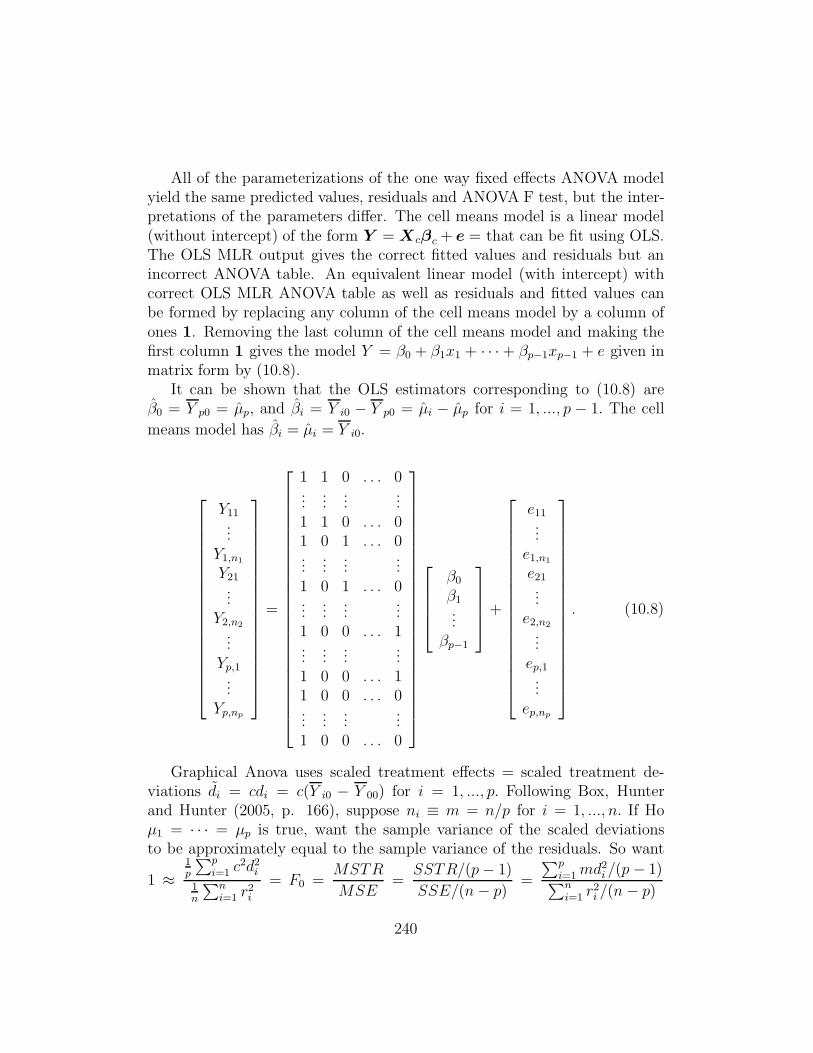
All of the parameterizations of the one way fixed effects ANOVA modelyield the same predicted values, residuals and ANOVA F test, but the inter-pretations of the parameters differ. The cell means model is a linear model(without intercept) of the form Y = Xcβc + e = that can be fit using OLS.The OLS MLR output gives the correct fitted values and residuals but anincorrect ANOVA table. An equivalent linear model (with intercept) withcorrect OLS MLR ANOVA table as well as residuals and fitted values canbe formed by replacing any column of the cell means model by a column ofones 1. Removing the last column of the cell means model and making thefirst column 1 gives the model Y = β0 + β1x1 + · · · + βp−1xp−1 + e given inmatrix form by (10.8).

It can be shown that the OLS estimators corresponding to (10.8) areβ0 = Y p0 = µp, and βi = Y i0 − Y p0 = µi − µp for i = 1, ..., p − 1. The cell

means model has βi = µi = Y i0.

Y11...

Y1,n1

Y21...

Y2,n2

...Yp,1...

Yp,np

=

1 1 0 . . . 0...

......

...1 1 0 . . . 01 0 1 . . . 0...

......

...1 0 1 . . . 0...

......

...1 0 0 . . . 1...

......

...1 0 0 . . . 11 0 0 . . . 0...

......

...1 0 0 . . . 0

β0

β1...

βp−1

+

e11...

e1,n1

e21...

e2,n2

...ep,1...

ep,np

. (10.8)

Graphical Anova uses scaled treatment effects = scaled treatment de-viations di = cdi = c(Y i0 − Y 00) for i = 1, ..., p. Following Box, Hunterand Hunter (2005, p. 166), suppose ni ≡ m = n/p for i = 1, ..., n. If Hoµ1 = · · · = µp is true, want the sample variance of the scaled deviationsto be approximately equal to the sample variance of the residuals. So want

1 ≈1p

∑p

i=1 c2d2i

1n

∑ni=1 r2

i

= F0 =MSTR

MSE=

SSTR/(p − 1)

SSE/(n − p)=

∑p

i=1 md2i /(p − 1)

∑n

i=1 r2i /(n − p)

240

since SSTR =∑p

i=1 m(Y i0 − Y 00)2 =

∑p

i=1 md2i . So

F0 =

∑p

i=1 c2 npd2

i∑n

i=1 r2i

=

∑p

i=1m(n−p)

p−1d2

i∑n

i=1 r2i

.

Equating numerators gives

c2 =mp

n

(n − p)

(p − 1)=

(n − p)

(p − 1)

since mp/n = 1. Thus c =√

(n − p)/(p − 1).For Graphical Anova, see Box, Hunter and Hunter (2005, p. 136, 150,

164, 166) and Hoaglin, Mosteller, and Tukey (1991). The R package granova,available from (http://streaming.stat.iastate.edu/CRAN/) and authored byR.M. Pruzek and J.E. Helmreich, may be useful.

The modified power transformation family

Yi = tλ(Zi) ≡ Z(λ)i =

Zλi − 1

λ

for λ 6= 0 and t0(Zi) = log(Zi) for λ = 0 where λ ∈ ΛL.Box and Cox (1964) give a numerical method for selecting the response

transformation for the modified power transformations. Although the methodgives a point estimator λo, often an interval of “reasonable values” is gen-erated (either graphically or using a profile likelihood to make a confidenceinterval), and λ ∈ ΛL is used if it is also in the interval.

There are several reasons to use a coarse grid ΛL of powers. First, severalof the powers correspond to simple transformations such as the log, squareroot, and reciprocal. These powers are easier to interpret than λ = .28,for example. Secondly, if the estimator λn can only take values in ΛL, thensometimes λn will converge in probability to λ∗ ∈ ΛL. Thirdly, Tukey (1957)showed that neighboring modified power transformations are often very sim-ilar, so restricting the possible powers to a coarse grid is reasonable.

The graphical method for response transformations is due to Olive (2004,2010: ch. 5). A variant of the method would plot the residual plot orboth the response and the residual plot for each of the five values of λ.Residual plots are also useful, but they do not distinguish between nonlinearmonotone relationships and nonmonotone relationships. See Fox (1991, p.55). Alternative methods are given by Cook and Olive (2001) and Box,Hunter and Hunter (2005, p. 321).

241

A randomization test for the one way ANOVA model has H0: thedifferent treatments have no effect. This null hypothesis is also true if all ppdfs Y |(W = ai) ∼ fZ(y − µ) are the same. An impractical randomizationtest uses all M = n!

n1!···np!ways of assigning ni of the Yij to treatment i for

i = 1, ..., p. Let F0 be the usual F statistic. The F statistic is computedfor each of the M permutations and H0 is rejected if the proportion of theM F statistics that are larger than F0 is less than δ. The distribution ofthe M F statistics is approximately Fp−1,n−p for large n when H0 is true.The power of the randomization test is also similar to that of the usual Ftest. See Hoeffding (1952). These results suggest that the usual F test issemiparametric: the pvalue is approximately correct if n is large and if all ppdfs Y |(W = ai) ∼ fZ(y − µ) are the same.

Let [x] be the integer part of x, eg [7.7] = 7. Olive (2011b) shows thatpractical randomization tests that use a random sample of max(1000, [n log(n)])permutations have level and power similar to the tests that use all M possi-ble permutations. See Ernst (2009) and the mpack function rand1way for Rcode.

Another alternative to one way ANOVA is to use feasible weighted leastsquares (FWLS) on the cell means model with σ2V = diag(σ2

1, ..., σ2p) where

σ2i is the variance of the ith group for i = 1, ..., p. Then V = diag(S2

1 , ..., S2p)

where S2i = 1

ni−1

∑ni

j=1(Yij − Y i0)2 is the sample variance of the Yij . Hence

the estimated weights for FWLS are wij ≡ wi = 1/S2i . Then the FWLS cell

means model has Y = Xcβc+e as in (10.4) except Cov(e) = diag(σ21, ..., σ

2p).

Hence Z = U cβc + ε. Then UTc U c = diag(n1w1, ..., npwp), (UT

c U c)−1 =

diag(S21/n1, ..., S

2p/np) = (XV

−1XT )−1, and UT

c Z = (w1Y10, ..., wpYp0)T .

ThusβFWLS = (Y 10, ..., Y p0)

T = βc.

That is, the FWLS estimator equals the one way ANOVA estimator of β

based on OLS applied to the cell means model. The ANOVA F test gener-alizes the pooled t test in that the two tests are equivalent for p = 2. TheFWLS procedure is also known as the Welch one way ANOVA and general-izes the Welch t test. The Welch t test is thought to be much better thanthe pooled t test. See Brown and Forsythe (1974ab), Kirk (1982, p. 100,101, 121, 122) and Welch (1947, 1951).

242

In matrix form Z = U cβc + ε becomes

√w1Y1,1

...√w1Y1,n1√w2Y21

...√w2Y2,n2

...√

wpYp,1...

√

wpYp,np

=

√w1 0 0 . . . 0...

......

...√w1 0 0 . . . 00

√w2 0 . . . 0

......

......

0√

w2 0 . . . 0...

......

...

0 0 0 . . .√

wp

......

......

0 0 0 . . .√

wp

µ1

µ2...

µp

+

ε11...

ε1,n1

ε21...

ε2,n2

...εp,1...

εp,np

.

(10.9)Four tests for Ho : µ1 = · · · = µp can be used if Rule of Thumb 10.3:

max(S1, ..., Sp) ≤ 2min(S1, ..., Sp) fails. Let Y = (Y1, ..., Yn)T , and let Y(1) ≤

Y(2) · · · ≤ Y(n) be the order statistics. Then the rank transformation of theresponse is Z = rank(Y ) where Zi = j if Yi = Y(j) is the jth order statistic.For example, if Y = (7.7, 4.9, 33.3, 6.6)T , then Z = (3, 1, 4, 2)T . The first testperforms the one way ANOVA F test with Z replacing Y . See Montgomery(1984, p. 117-118). Two of the next three tests are described in Brown andForsythe (1974b). Let dxe be the smallest integer ≥ x, eg d7.7e = 8. Thenthe Welch (1951) ANOVA F test uses test statistic

FW =

∑p

i=1 wi(Y i0 − Y00)2/(p − 1)

1 + 2(p−2)p2−1

∑p

i=1(1 − wi

u)2/(ni − 1)

where wi = ni/S2i , u =

∑p

i=1 wi and Y00 =∑p

i=1 wiY i0/u. Then the teststatistic is compared to an Fp−1,dW

distribution where dW = dfe and

1/f =3

p2 − 1

p∑

i=1

(1 − wi

u)2/(ni − 1).

For the modified Welch (1947) test, the test statistic is compared to anFp−1,dMW

distribution where dMW = dfe and

f =

∑p

i=1(S2i /ni)

2

∑p

i=11

ni−1(S2

i /ni)2=

∑p

i=1(1/wi)2

∑p

i=11

ni−1(1/wi)2

.

243

Some software uses f instead of dW or dMW , and variants on the denominatordegrees of freedom dW or dMW are common.

The modified ANOVA F test uses test statistic

FM =

∑p

i=1 ni(Y i0 − Y 00)2

∑pi=1(1 − ni

n)S2

i

The test statistic is compared to an Fp−1,dMdistribution where dM = dfe

and

1/f =

p∑

i=1

c2i /(ni − 1)

where

ci = (1 − ni

n)S2

i /[

p∑

i=1

(1 − ni

n)S2

i ].

The mpack function anovasim can be used to compare the five tests.

Huberty and Olejnik (2006) and Khattree and Naik (1999, ch. 4) are use-ful reference for MANOVA. Mardia (1971) notes that the one way MANOVAtest based on Pillai’s trace V is robust to nonnormality, especially when allof the treatment sample sizes are the same: ni ≡ h. Permutation tests offeran alternative. See, for example, Anderson (2001).

10.7 Problems

PROBLEMS WITH AN ASTERISK * ARE ESPECIALLY USE-FUL.

10.1∗. In the MANOVA model, βi = (XT X)−1XT Y i, and Y i = Xβi +ei. Treating Xβi as a constant, Cov(Y i, Y j) = Cov(ei, ej) = σijIn. Using

this information, show Cov(βi, βj) = σij(XT X)−1.

10.2. SAS Institute (1985, p. 498 - 501) describes a one way MANOVAmodel. There are two groups for gender: female and male. There were p = 4(skull measurements) variables X1 = length X2 = basilar, X3 = zygomatand X4 = postorb. There were n1 = 18 females and n2 = 22 males measured.Suppose t0 = 0.9567 and pvalue = 0.6566. Here to was Wilk’s lambda, butthe other three test statistics gave the same pvalue. Do a 4 step one wayMANOVA test.

244

10.3. Suppose the 15 units are 1 Adatorwovor, 2 Adhikari, 3 Alanzi, 4Alsibiani, 5 AlTalib, 6 Fan, 7 Kuo, 8 Lamsal, 9 Liu, 10 Meyer, 11 Peiris,12 Rathnayake, 13 Rupasinghe, 14 Schroeppel and 15 Watagoda. Use thefollowing output to allocate the 15 units to three groups of 5. Show the threegroups.

> sample(15)

[1] 6 3 4 2 1 10 7 5 12 15 13 8 14 11 9

R/Splus Problems

Warning: Use the command source(“G:/mpack.txt”) to downloadthe programs. See Preface or Section 15.2. Typing the name of thempack function, eg ddplot, will display the code for the function. Use theargs command, eg args(ddplot), to display the needed arguments for thefunction.

10.4. The Johnson and Wichern (1988, p. 262) turtle data gives thelength, width and height of painted turtle shells. There is a sample of 24female and a sample of 24 male turtles.

a) The R command for this part make the response and residual plots foreach of the three variables. Click the rightmost mouse button and highlightStop to advance the plot. When you have the response and residual plots forone variable on the screen, copy and paste the two plots into Word. Do thisthree times, once for each variable. The male turtles are smaller than thefemale turtles.

b) The R command for this plot makes a DD plot of the residuals andadds the lines corresponding to the three prediction regions of Section 5.2.The robust cutoff is larger than the semiparametric cutoff. Place the plot inWord. Do the residuals appear to follow a multivariate normal distribution?

245