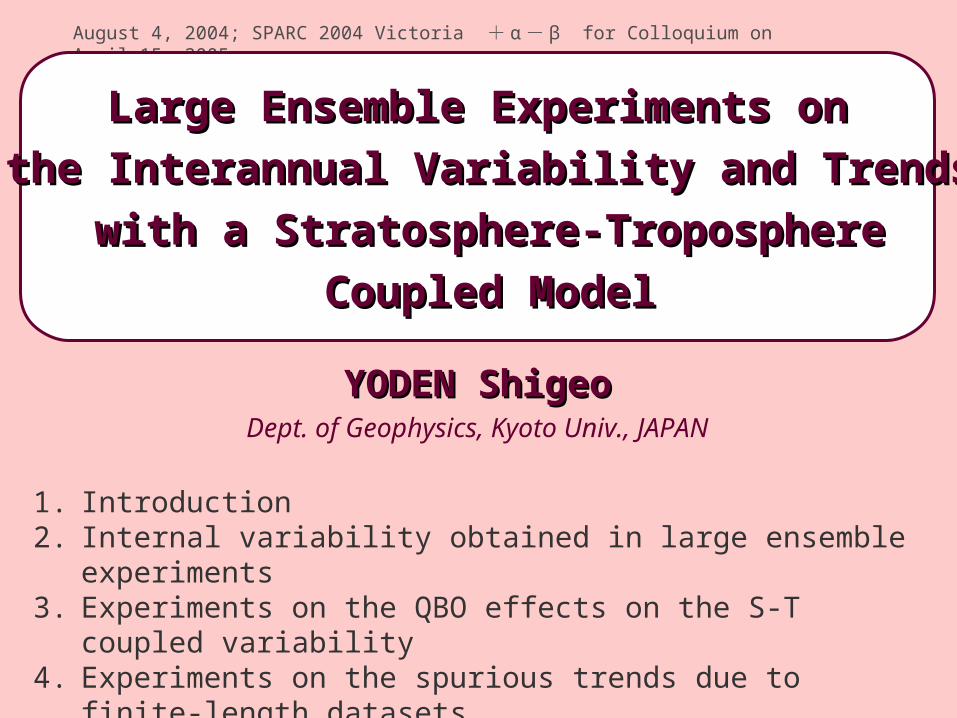
YODEN ShigeoYODEN ShigeoDept. of Geophysics, Kyoto Univ., JAPAN

August 4, 2004; SPARC 2004 Victoria　＋ α－ β for Colloquium on April 15, 2005

1. Introduction2. Internal variability obtained in large ensemble

experiments 3. Experiments on the QBO effects on the S-T coupled

variability4. Experiments on the spurious trends due to finite-length

datasets5. Concluding Remarks

Large Ensemble Experiments onLarge Ensemble Experiments on

the Interannual Variability and Trendsthe Interannual Variability and Trends

with a Stratosphere-Tropospherewith a Stratosphere-Troposphere

Coupled ModelCoupled Model

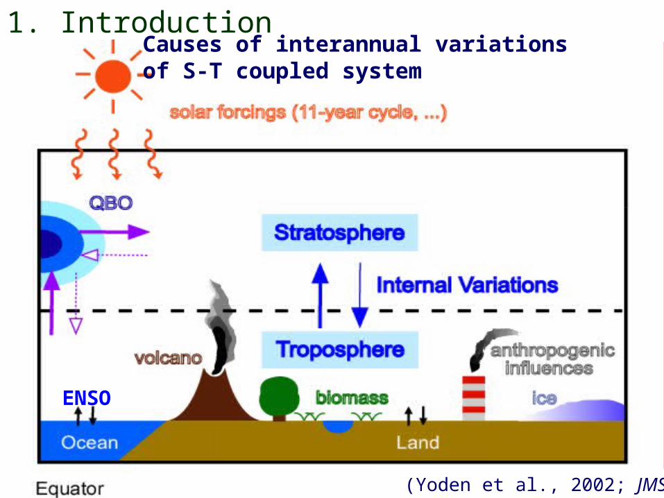
1. IntroductionCauses of interannual variations of S-T coupled system

(Yoden et al., 2002; JMSJ )

ENSO

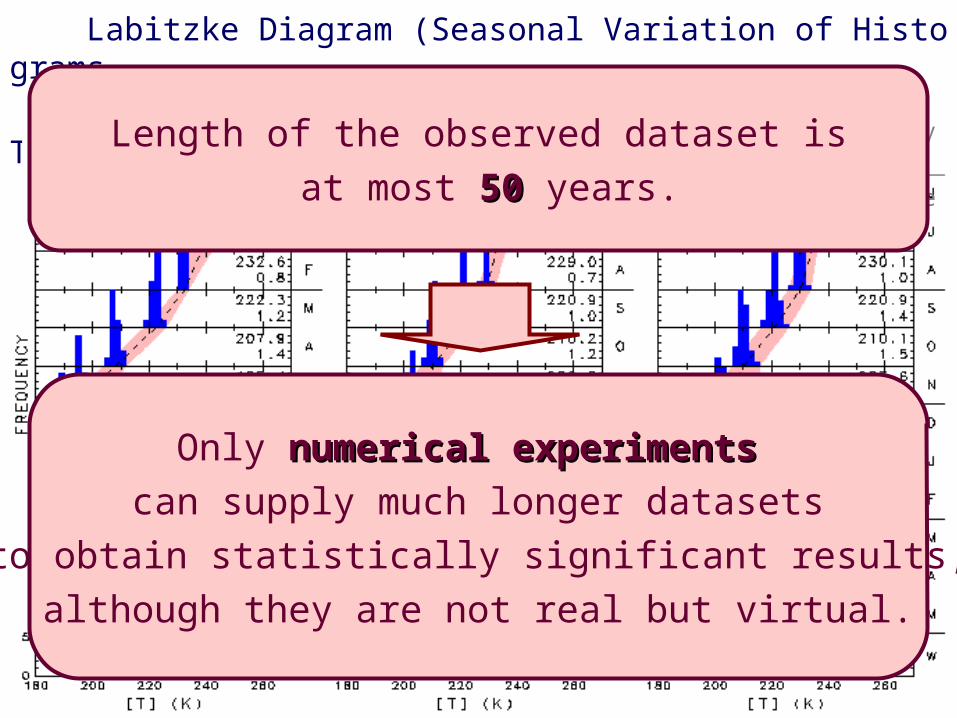
Labitzke Diagram (Seasonal Variation of Histograms

of the Monthly Mean Temperature; at 30 hPa)

South Pole(NCEP)

North Pole(NCEP)

North Pole(Berlin)

courtesy ofDr. Labitzke

Length of the observed dataset is at most 5050 years.

Only numerical experimentsnumerical experiments can supply much longer datasets

to obtain statistically significant results,although they are not real but virtual.

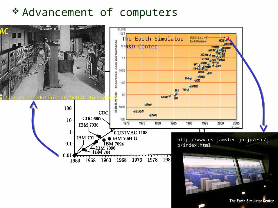
The Earth Simulator

R&D Center

Advancement of computers

http://www.es.jamstec.go.jp/esc/jp/index.html

ENIAC

http://ei.cs.vt.edu/~history/ENIAC.Richey.HTML

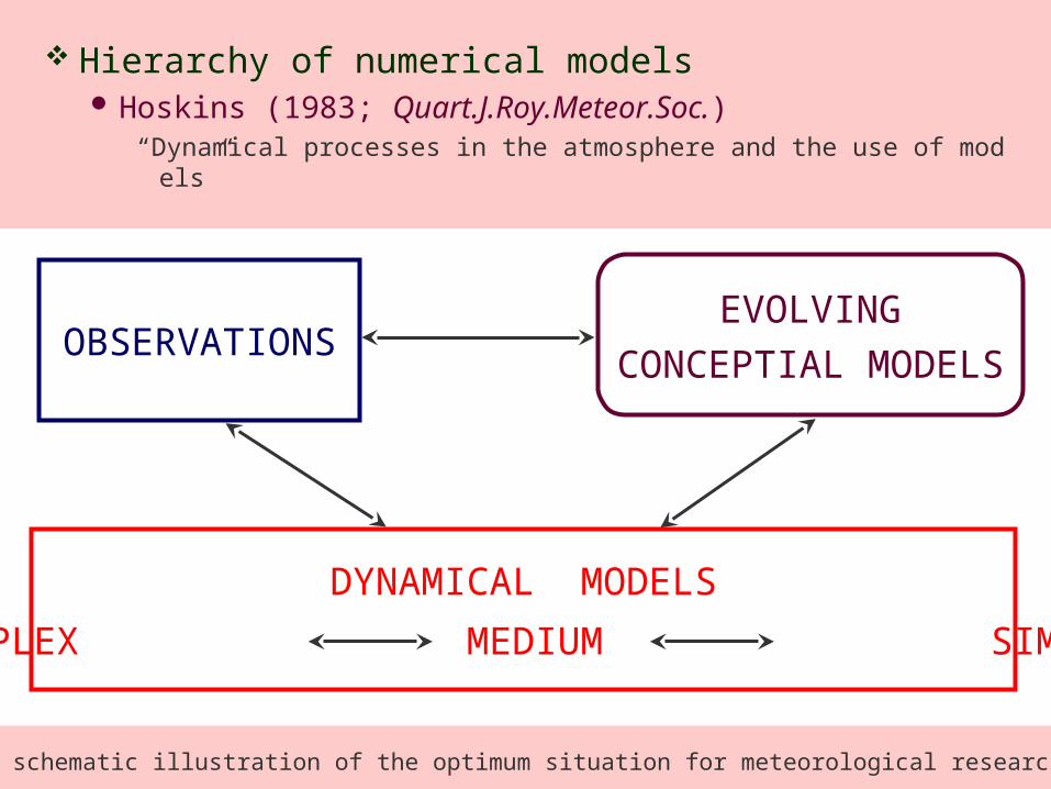
Hierarchy of numerical models Hoskins (1983; Quart.J.Roy.Meteor.Soc.)

“Dynamical processes in the atmosphere and the use of models”

OBSERVATIONS

DYNAMICAL MODELS

COMPLEX MEDIUM SIMPLE

EVOLVINGCONCEPTIAL MODELS

A schematic illustration of the optimum situation for meteorological research

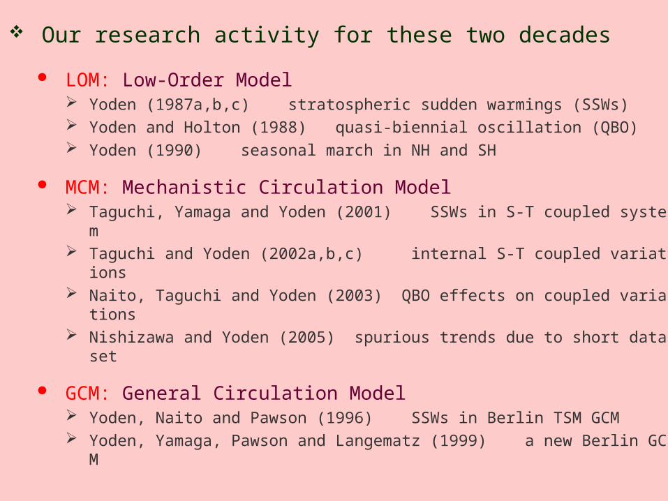
Our research activity for these two decades

LOM: Low-Order Model Yoden (1987a,b,c) stratospheric sudden warmings (SSWs) Yoden and Holton (1988) quasi-biennial oscillation (QBO) Yoden (1990) seasonal march in NH and SH

MCM: Mechanistic Circulation Model Taguchi, Yamaga and Yoden (2001) SSWs in S-T coupled system Taguchi and Yoden (2002a,b,c) internal S-T coupled variations Naito, Taguchi and Yoden (2003) QBO effects on coupled variations Nishizawa and Yoden (2005) spurious trends due to short dataset

GCM: General Circulation Model Yoden, Naito and Pawson (1996) SSWs in Berlin TSM GCM Yoden, Yamaga, Pawson and Langematz (1999) a new Berlin GCM

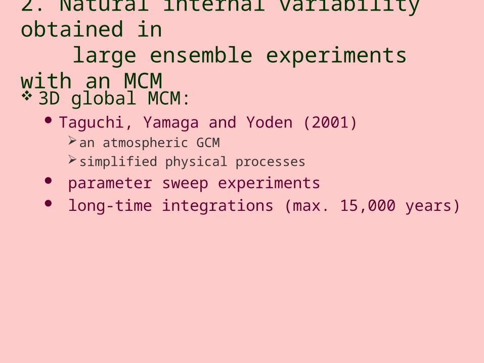
3D global MCM: Taguchi, Yamaga and Yoden (2001)

an atmospheric GCMsimplified physical processes

parameter sweep experiments long-time integrations (max. 15,000 years)

2. Natural internal variability obtained in large ensemble experiments with an MCM

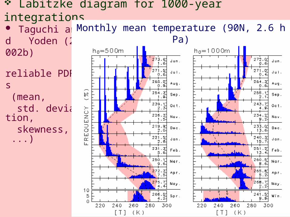
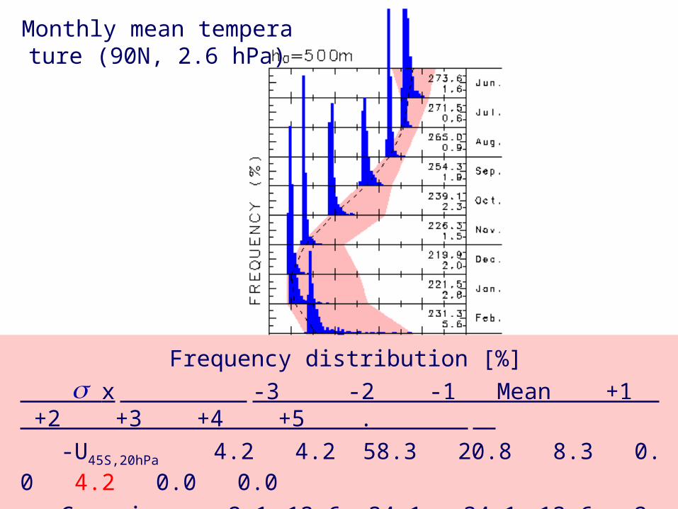
Labitzke diagram for 1000-year integrations Taguchi and Yoden (2002b)

reliable PDFs (mean, std. deviation, skewness, ...)

Monthly mean temperature (90N, 2.6 hPa)

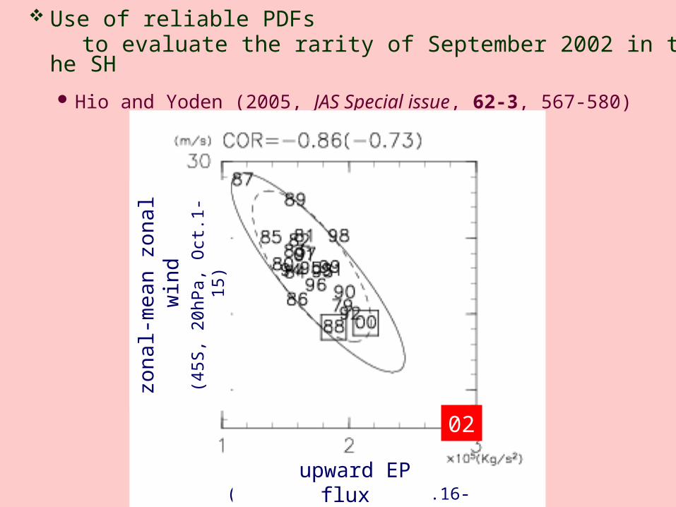
Use of reliable PDFs to evaluate the rarity of September 2002 in the SH

Hio and Yoden (2005, JAS Special issue, 62-3, 567-580)

02

zona

l-mea

n zo

nal w

ind

(45S

, 20

hPa,

Oct

.1-1

5)

(45-75S, 100hPa, Aug.16-Sep.30) upward EP flux

Monthly mean temperature (90N, 2.6 hPa)

Frequency distribution [%]

x 　　 -3 -2 -1 Mean +1 +2 +3 +4 +5 . 　 -U45S,20hPa 4.2 4.2 58.3 20.8 8.3 0.0 4.2 0.0 0.0

Gaussian 2.1 13.6 34.1 34.1 13.6 2.1 0.1 3x10-3 -

T&Y(Feb.) 0.3 8.7 47.7 32.8 7.0 1.8 1.1 0.2 0.2

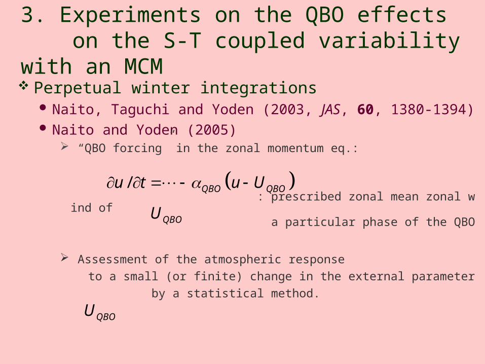
3. Experiments on the QBO effects on the S-T coupled variability with an MCM Perpetual winter integrations

Naito, Taguchi and Yoden (2003, JAS, 60, 1380-1394) Naito and Yoden (2005)

“QBO forcing” in the zonal momentum eq.:

: prescribed zonal mean zonal wind of a particular phase of the QBO

Assessment of the atmospheric response to a small (or finite) change in the external parameter by a statistical method.

/ QBO QBOu t u U

QBOU

QBOU

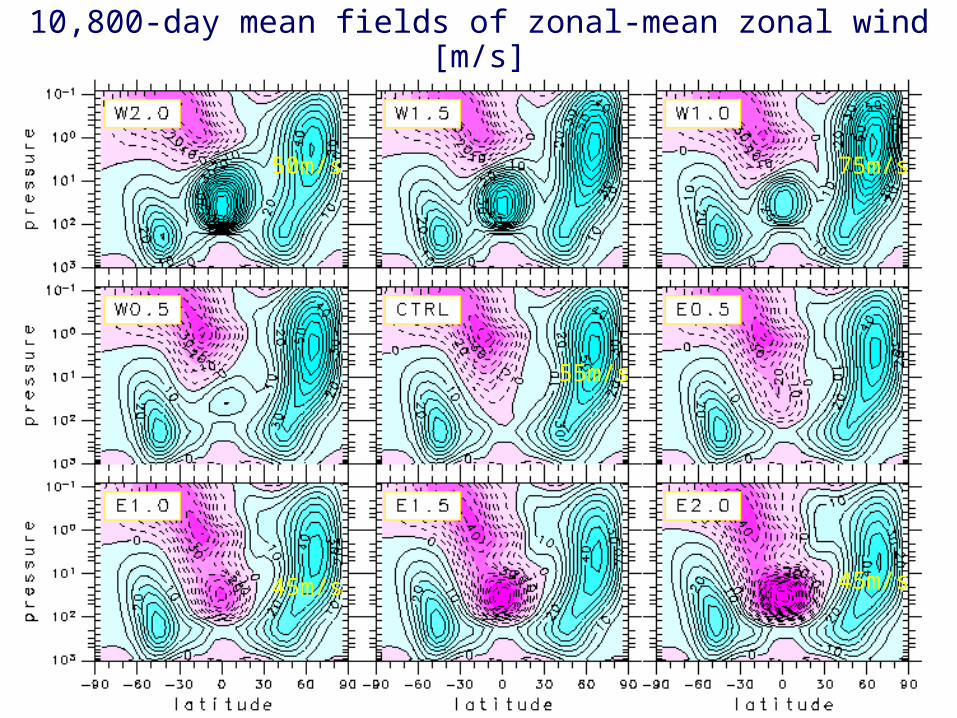
10,800-day mean fields of zonal-mean zonal wind [m/s]

75m/s50m/s

55m/s

45m/s 45m/s

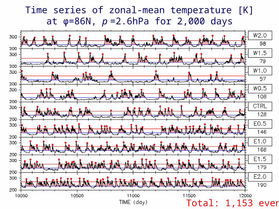
Time series of zonal-mean temperature [K]at φ=86N, p =2.6hPa for 2,000 days

Total: 1,153 events

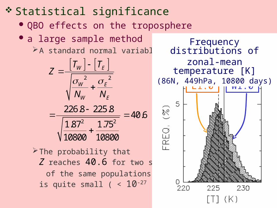
Statistical significance QBO effects on the troposphere a large sample method

A standard normal variable:

The probability thatZ reaches 40.6 for two samples

of the same populationsis quite small ( < 10-27 )

E1.0 W1.0

Frequency distributions ofzonal-mean temperature [K]

(86N, 449hPa, 10800 days) 2 2

2 2

226.8 225.840.6

1.87 1.75

10800 10800

W E

W E

W E

T TZ

N N

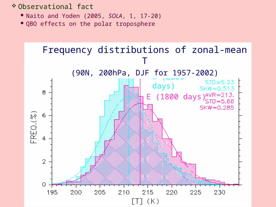
Observational fact Naito and Yoden (2005, SOLA, 1, 17-20) QBO effects on the polar troposphere

W (2250 days)

E (1800 days)

Frequency distributions of zonal-mean T(90N, 200hPa, DJF for 1957-2002)

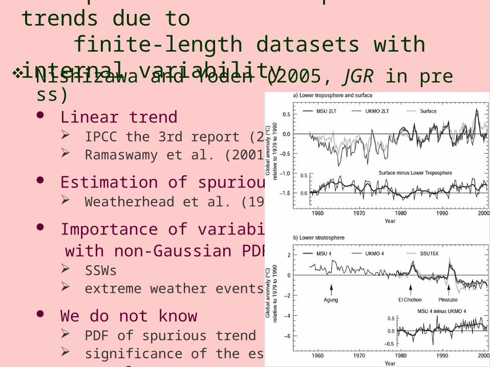
4. Experiments on the spurious trends due to finite-length datasets with internal variability Nishizawa and Yoden (2005, JGR in press)

Linear trend IPCC the 3rd report (2001) Ramaswamy et al. (2001)

Estimation of spurious trend Weatherhead et al. (1998)

Importance of variability with non-Gaussian PDF

SSWs extreme weather events

We do not know PDF of spurious trend significance of the estimated value

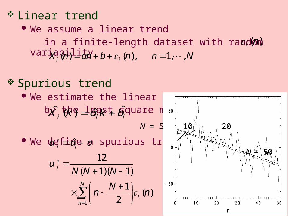
Linear trend We assume a linear trend in a finite-length dataset with random

variability

Spurious trend We estimate the linear trend by the least square method

We define a spurious trend as

( ) ( ), 1, ,i iX n an b n n N

ˆˆ ˆ( )i i iX k a k b

1

ˆ'

12'

( 1)( 1)

1( )

2

i i

i

N

in

a a a

aN N N

Nn n　 　 　

( )i n

N = 5 10 20

N = 50

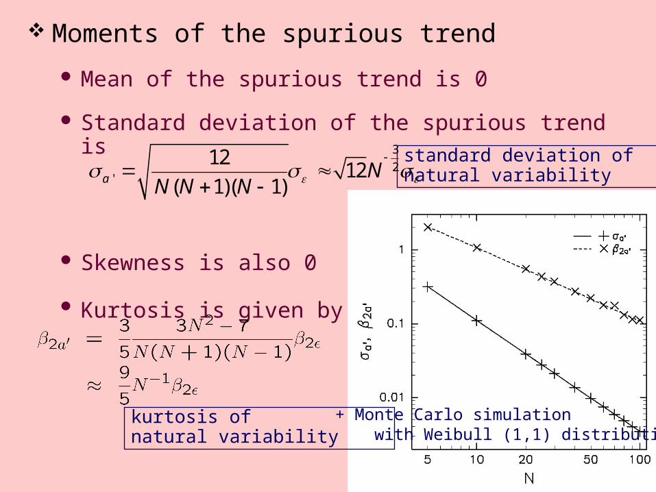
Moments of the spurious trend Mean of the spurious trend is 0

Standard deviation of the spurious trend is

Skewness is also 0

Kurtosis is given by

3

2'

1212

( 1)( 1)a NN N N

standard deviation ofnatural variability

kurtosis ofnatural variability

+ Monte Carlo simulation with Weibull (1,1) distribution

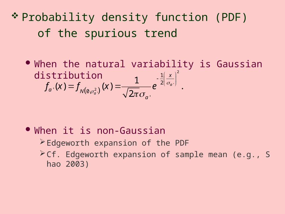
Probability density function (PDF) of the spurious trend

When the natural variability is Gaussian distribution

When it is non-GaussianEdgeworth expansion of the PDF Cf. Edgeworth expansion of sample mean (e.g., Shao 2003)

2

'2

'

1

2' 0,

'

1( ) ( ) .

2a

a

x

a Na

f x f x e

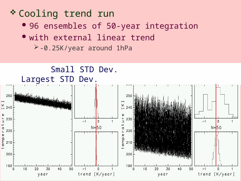
Cooling trend run 96 ensembles of 50-year integration with external linear trend

-0.25K/year around 1hPa

Small STD Dev. Largest STD Dev.

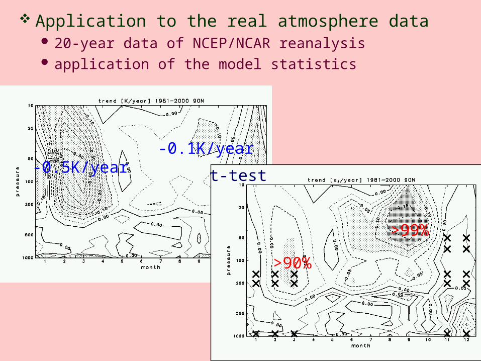
Application to the real atmosphere data 20-year data of NCEP/NCAR reanalysis application of the model statistics

-0.1K/year-0.5K/year

+0.1K/yeart-test

>99%

>90%

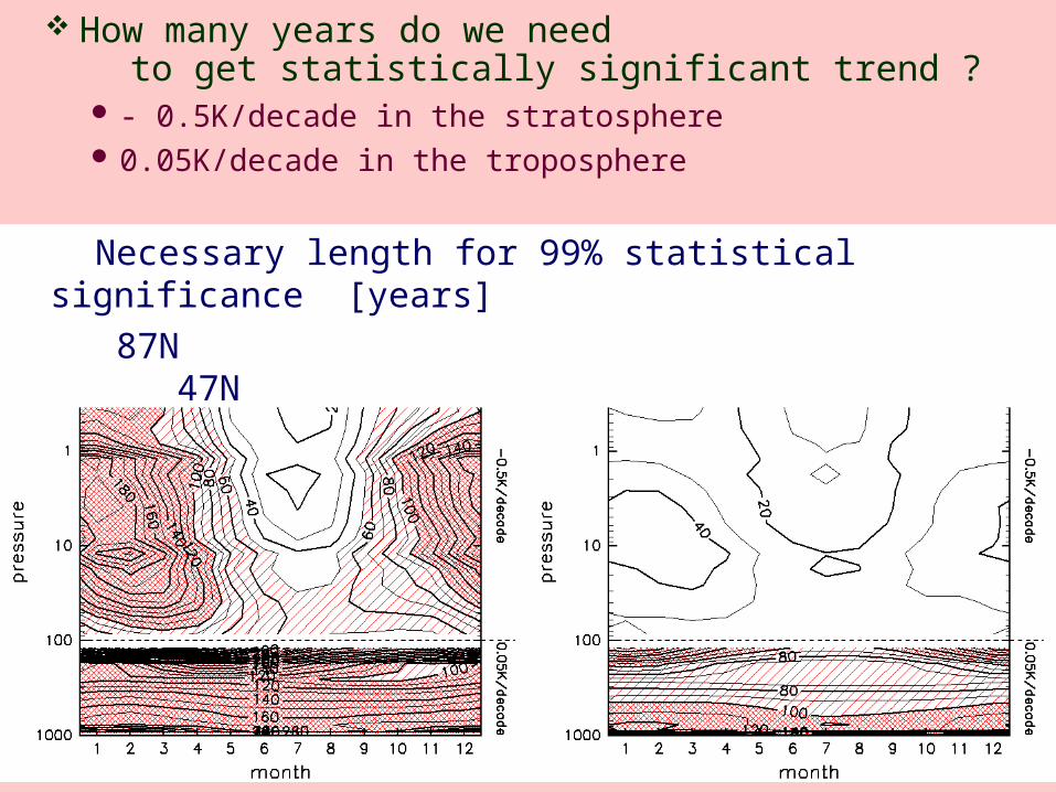
Necessary length for 99% statistical significance [years]

87N 47N

How many years do we need to get statistically significant trend ?

- 0.5K/decade in the stratosphere 0.05K/decade in the troposphere

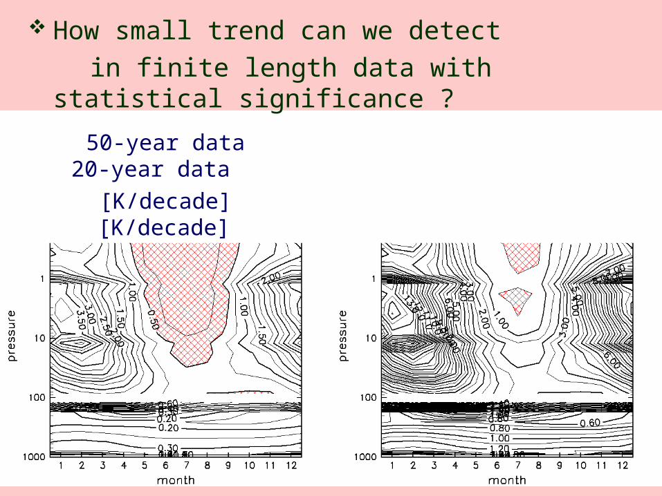
50-year data 20-year data

[K/decade] [K/decade]

How small trend can we detect in finite length data with statistical

significance ?

Recent advancement in computing facilities has enabled us to do some parameter sweep experiments with 3D MCMs

Very long-time integrations give reliable PDFs (non-Gaussian, bimodal, .... ), which might be important for nonlinear perspectives in climate-change studies

Atmospheric response to small change in an external parameter (e.g., QBO, solar cycle, …) can be statistically assessed by a large sample method

5. Concluding Remarks