Log Covariance Matrix Estimation

Xinwei Deng

Department of Statistics

University of Wisconsin-Madison

Joint work with Kam-Wah Tsui (Univ. of Wisconsin-Madsion)

1

Outline

• Background and Motivation

• The Proposed Log-ME Method

• Simulation and Real Example

• Summary and Discussion

2

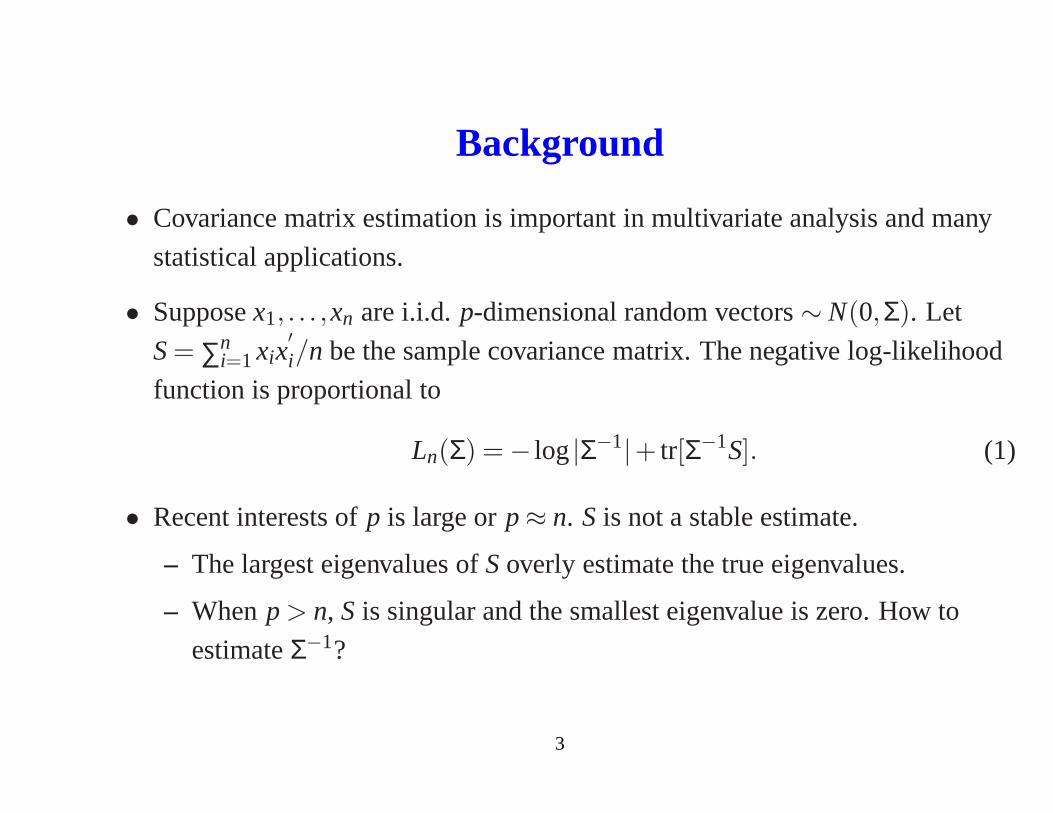
Background

• Covariance matrix estimation is important in multivariateanalysis and many

statistical applications.

• Supposex1, . . . ,xn are i.i.d.p-dimensional random vectors∼ N(0,Σ). Let

S= ∑ni=1 xix

′i/n be the sample covariance matrix. The negative log-likelihood

function is proportional to

Ln(Σ) = − log|Σ−1|+ tr[Σ−1S]. (1)

• Recent interests ofp is large orp≈ n. S is not a stable estimate.

– The largest eigenvalues ofSoverly estimate the true eigenvalues.

– Whenp > n, S is singular and the smallest eigenvalue is zero. How to

estimateΣ−1?

3

Recent Estimation Methods onΣ or Σ−1

• Reduce number of nonzeros estimates ofΣ or Σ−1.

– Σ: Bickel and Levina (2008), using thresholding.

– Σ−1: Yuan and Lin (2007),l1 penalty onΣ−1.

Friedman et al., (2008), Graphical Lasso.

Meinshausen and Buhlmann (2006), Reformulated as regression.

• Shrinkage estimates of the covariance matrix.

– Ledoit and Wolf (2006),ρΣ+(1−ρ)µI.

– Won et al. (2009), control the condition number (largest

eigenvalue/smallest eigenvalue).

4

Motivation

• Estimate ofΣ or Σ−1 needs to be positive definite.

– The mathematical restriction makes the covariance matrix estimation

problem challenging.

• Any positive definiteΣ can be expressed as a matrix exponential of a real

symmetric matrixA.

Σ = exp(A) = I +A+A2

2!+ · · ·

– Expressing the likelihood function in terms ofA≡ log(Σ) releases the

mathematical restriction.

• Consider the spectral decomposition ofΣ = TDT′ with D = diag(d1, . . . ,dp).

ThenA = TMT′ with M = diag(log(d1), . . . , log(dp)).

5

Idea of the Proposed Method

• Leonard and Hsu (1992) used this log-transformation methodto estimateΣ by

approximating the likelihood using Volterra integral equation.

– Their approximation based on onSbeing nonsingular⇒ not applicable

whenp≥ n.

• We extend the likelihood approximation to the case of singular S.

• Regularize the largest and smallest eigenvalues ofΣ simultaneously.

• An efficient iterative quadratic programming algorithm to estimateA (log Σ).

• Call the resulting estimate “Log-ME”, Logarithm-transformed Matrix

Estimate.

6

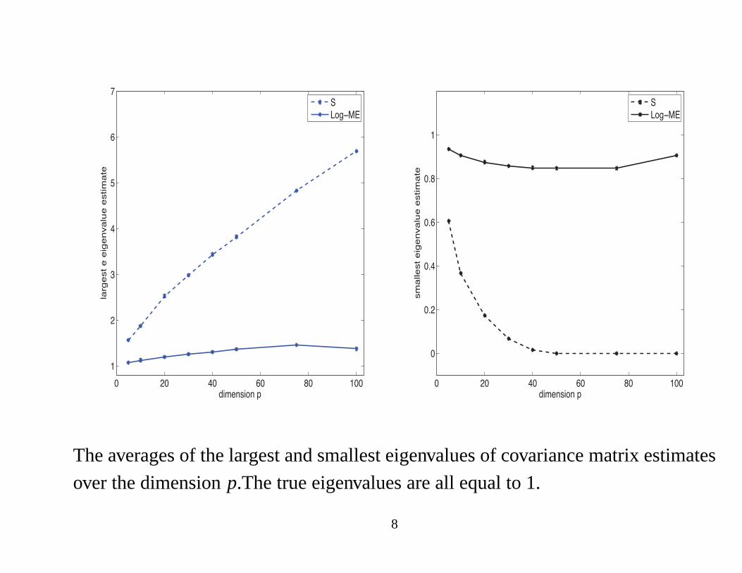
A Simple Example

• Experiment: simulatexi ’s from N(0, I), i = 1, . . . ,n wheren = 50.

• For eachp varying from 5 to 100, consider the the largest and smallest

eigenvalues of the covariance matrix estimate.

• For eachp, repeat the experiment 100 times and compute the average of the

largest eigenvalues and the average of the smallest eigenvalues for

– The sample covariance matrix.

– The Log-ME covariance matrix estimate

7

! "! #! $! %! &!!

&

"

'

#

(

$

)

*+,-./+0.12

3456-/71-1-+6-.8439-1-/7+,47-

1

1:

;06!<=

! "! #! $! %! &!!

!

!'"

!'#

!'$

!'%

&

()*+,-).,/0

-*122+-3/+)4+,5126+/+-3)*13+

/

/7

8.4!9:

The averages of the largest and smallest eigenvalues of covariance matrix estimates

over the dimensionp.The true eigenvalues are all equal to 1.

8

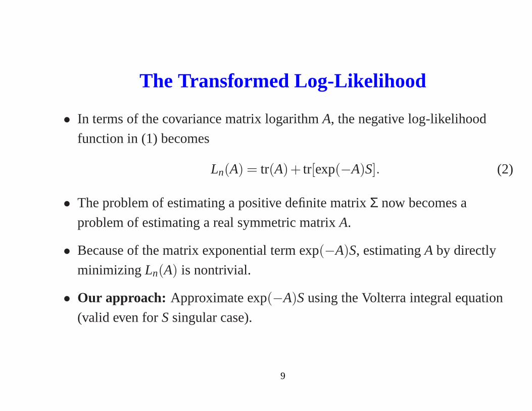
The Transformed Log-Likelihood

• In terms of the covariance matrix logarithmA, the negative log-likelihood

function in (1) becomes

Ln(A) = tr(A)+ tr[exp(−A)S]. (2)

• The problem of estimating a positive definite matrixΣ now becomes a

problem of estimating a real symmetric matrixA.

• Because of the matrix exponential term exp(−A)S, estimatingA by directly

minimizingLn(A) is nontrivial.

• Our approach: Approximate exp(−A)Susing the Volterra integral equation

(valid even forSsingular case).

9

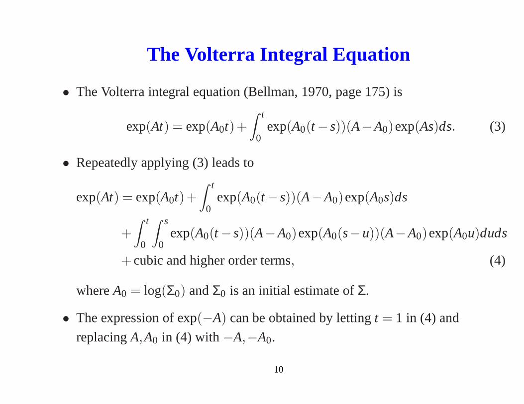
The Volterra Integral Equation

• The Volterra integral equation (Bellman, 1970, page 175) is

exp(At) = exp(A0t)+

∫ t

0exp(A0(t −s))(A−A0)exp(As)ds. (3)

• Repeatedly applying (3) leads to

exp(At) = exp(A0t)+∫ t

0exp(A0(t −s))(A−A0)exp(A0s)ds

+

∫ t

0

∫ s

0exp(A0(t −s))(A−A0)exp(A0(s−u))(A−A0)exp(A0u)duds

+cubic and higher order terms, (4)

whereA0 = log(Σ0) andΣ0 is an initial estimate ofΣ.

• The expression of exp(−A) can be obtained by lettingt = 1 in (4) and

replacingA,A0 in (4) with−A,−A0.

10

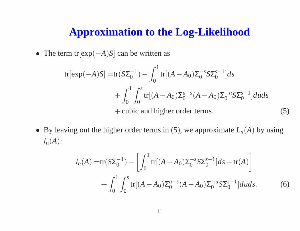
Approximation to the Log-Likelihood

• The term tr[exp(−A)S] can be written as

tr[exp(−A)S] =tr(SΣ−10 )−

∫ 1

0tr[(A−A0)Σ−s

0 SΣs−10 ]ds

+∫ 1

0

∫ s

0tr[(A−A0)Σu−s

0 (A−A0)Σ−u0 SΣs−1

0 ]duds

+cubic and higher order terms. (5)

• By leaving out the higher order terms in (5), we approximateLn(A) by using

ln(A):

ln(A) =tr(SΣ−10 )−

[

∫ 1

0tr[(A−A0)Σ−s

0 SΣs−10 ]ds− tr(A)

]

+∫ 1

0

∫ s

0tr[(A−A0)Σu−s

0 (A−A0)Σ−u0 SΣs−1

0 ]duds. (6)

11

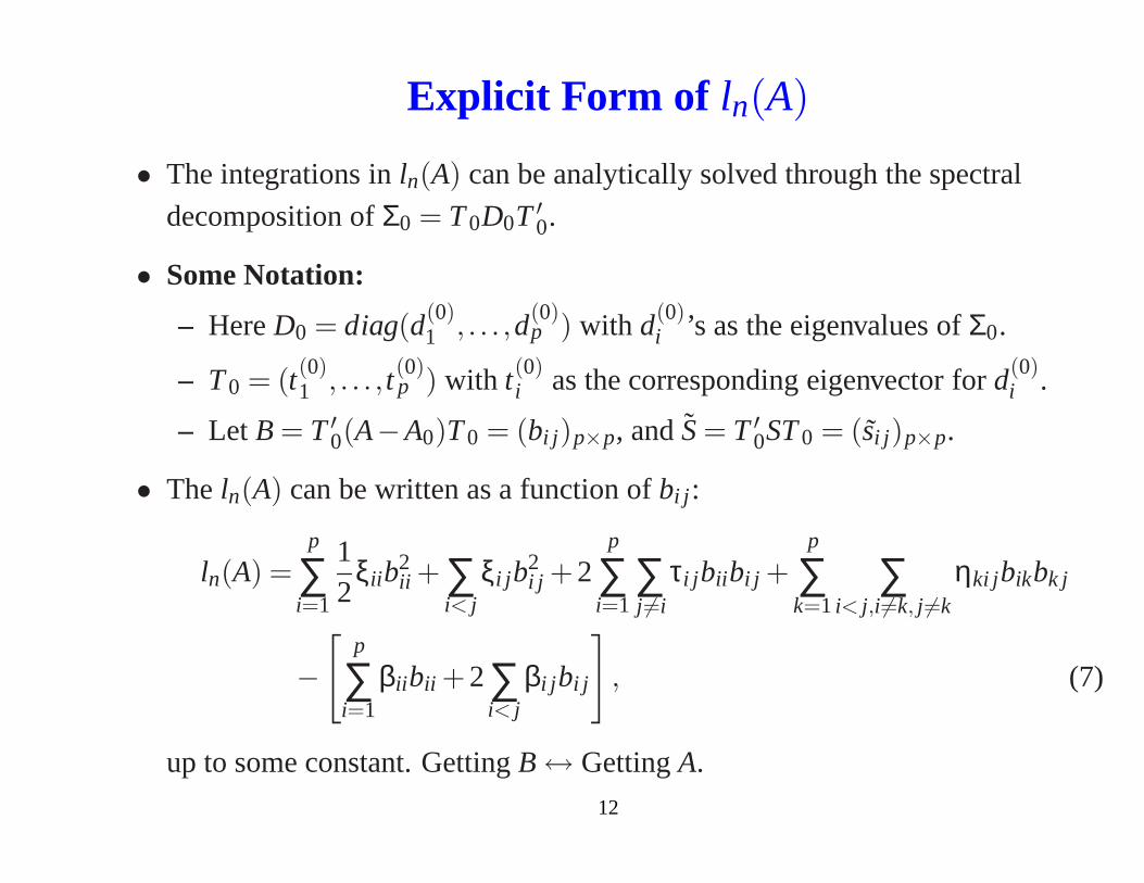
Explicit Form of ln(A)

• The integrations inln(A) can be analytically solved through the spectral

decomposition ofΣ0 = T0D0T ′0.

• Some Notation:

– HereD0 = diag(d(0)1 , . . . ,d(0)

p ) with d(0)i ’s as the eigenvalues ofΣ0.

– T0 = (t(0)1 , . . . , t(0)

p ) with t(0)i as the corresponding eigenvector ford(0)

i .

– Let B = T ′0(A−A0)T0 = (bi j )p×p, andS= T ′

0ST0 = (si j )p×p.

• The ln(A) can be written as a function ofbi j :

ln(A) =p

∑i=1

12

ξii b2ii + ∑

i< jξi j b

2i j +2

p

∑i=1

∑j 6=i

τi j bii bi j +p

∑k=1

∑i< j,i6=k, j 6=k

ηki jbikbk j

−[

p

∑i=1

βii bii +2∑i< j

βi j bi j

]

, (7)

up to some constant. GettingB↔ GettingA.

12

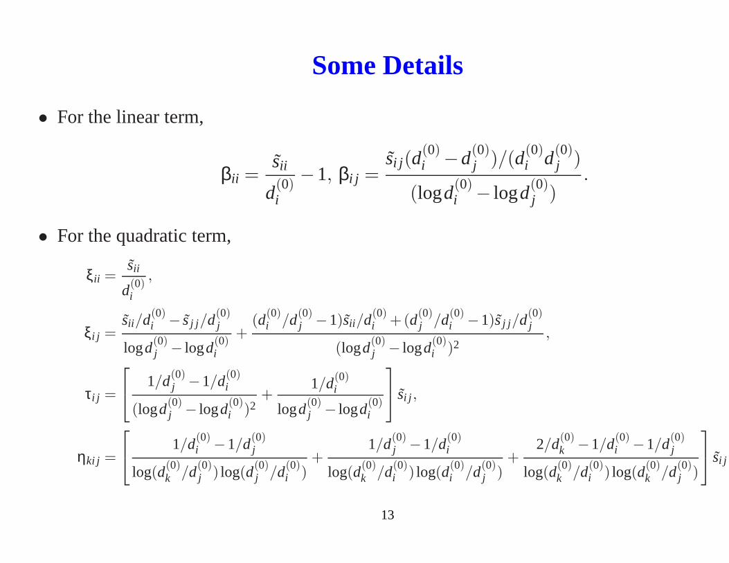
Some Details

• For the linear term,

βii =sii

d(0)i

−1, βi j =si j (d

(0)i −d(0)

j )/(d(0)i d(0)

j )

(logd(0)i − logd(0)

j ).

• For the quadratic term,

ξii =sii

d(0)i

,

ξi j =sii /d(0)

i − sj j /d(0)j

logd(0)j − logd(0)

i

+(d(0)

i /d(0)j −1)sii /d(0)

i +(d(0)j /d(0)

i −1)sj j /d(0)j

(logd(0)j − logd(0)

i )2,

τi j =

1/d(0)j −1/d(0)

i

(logd(0)j − logd(0)

i )2+

1/d(0)i

logd(0)j − logd(0)

i

si j ,

ηki j =

1/d(0)i −1/d(0)

j

log(d(0)k /d(0)

j ) log(d(0)j /d(0)

i )+

1/d(0)j −1/d(0)

i

log(d(0)k /d(0)

i ) log(d(0)i /d(0)

j )+

2/d(0)k −1/d(0)

i −1/d(0)j

log(d(0)k /d(0)

i ) log(d(0)k /d(0)

j )

si j .

13

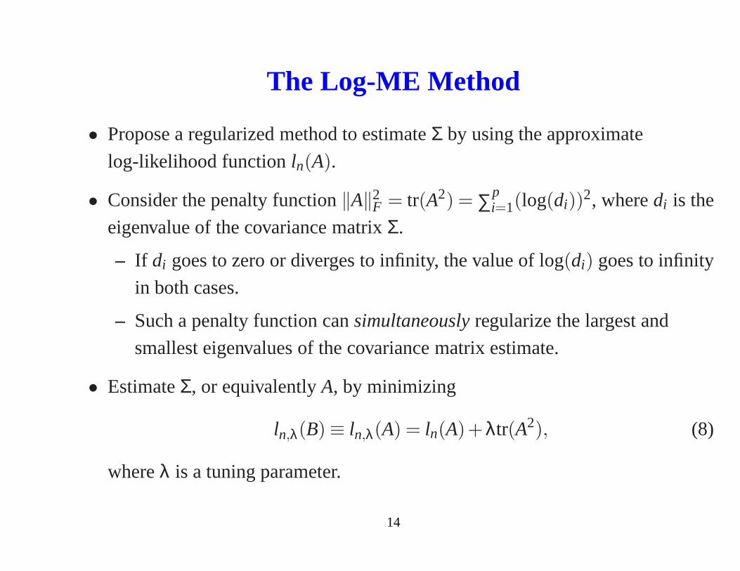
The Log-ME Method

• Propose a regularized method to estimateΣ by using the approximate

log-likelihood functionln(A).

• Consider the penalty function‖A‖2F = tr(A2) = ∑p

i=1(log(di))2, wheredi is the

eigenvalue of the covariance matrixΣ.

– If di goes to zero or diverges to infinity, the value of log(di) goes to infinity

in both cases.

– Such a penalty function cansimultaneouslyregularize the largest and

smallest eigenvalues of the covariance matrix estimate.

• EstimateΣ, or equivalentlyA, by minimizing

ln,λ(B) ≡ ln,λ(A) = ln(A)+λtr(A2), (8)

whereλ is a tuning parameter.

14

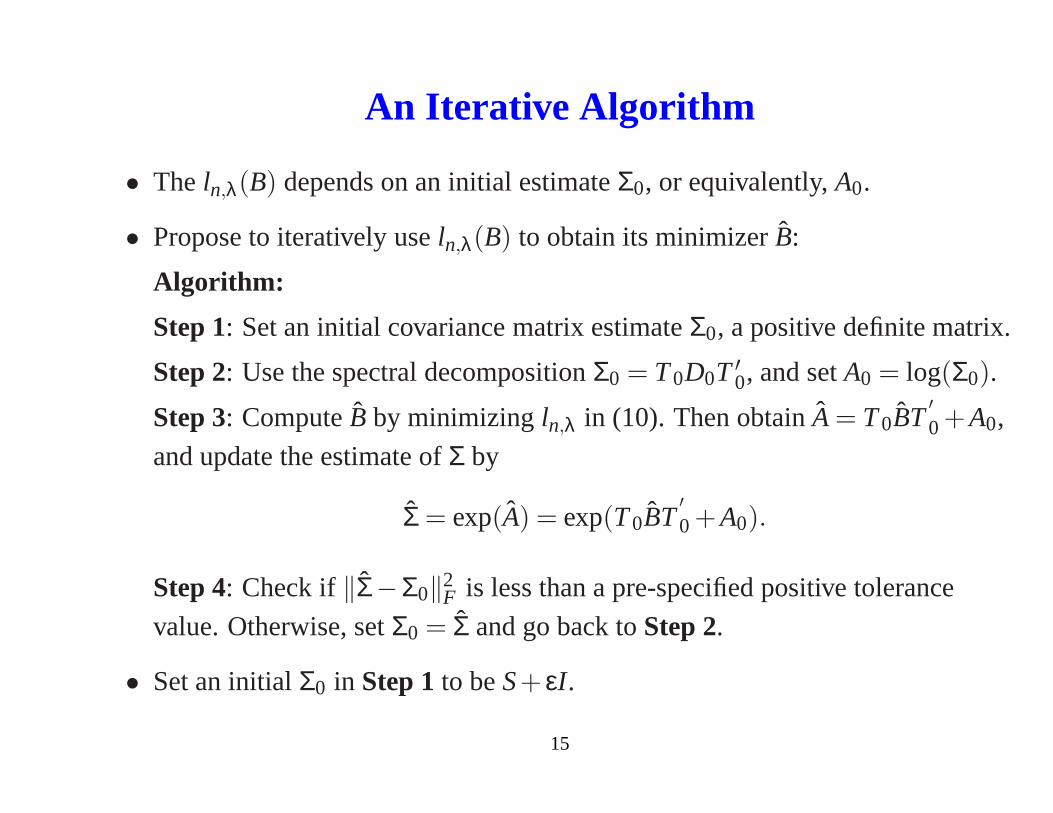
An Iterative Algorithm

• The ln,λ(B) depends on an initial estimateΣ0, or equivalently,A0.

• Propose to iteratively useln,λ(B) to obtain its minimizerB:

Algorithm:

Step 1: Set an initial covariance matrix estimateΣ0, a positive definite matrix.

Step 2: Use the spectral decompositionΣ0 = T0D0T ′0, and setA0 = log(Σ0).

Step 3: ComputeB by minimizing ln,λ in (10). Then obtainA = T0BT′0 +A0,

and update the estimate ofΣ by

Σ = exp(A) = exp(T0BT′0 +A0).

Step 4: Check if‖Σ−Σ0‖2F is less than a pre-specified positive tolerance

value. Otherwise, setΣ0 = Σ and go back toStep 2.

• Set an initialΣ0 in Step 1to beS+ εI .

15

Simulation Study• Six different covariance models ofΣ = (σi j )p×p are used for comparison,

– Model 1: Homogeneous model withΣ = I .

– Model 2: MA(1) model withσii = 1,σi,i−1 = σi−1,i = 0.45.

– Model 3: Circle model withσii = 1,σi,i−1 = σi−1,i = 0.3,σ1,p = σp,1 = 0.3.

• Compare four estimation methods: the banding estimate (Bickel and Levina,2008), the LW estimate (Ledoit and Wolf, 2006), the Glasso estimate (Yuanand Lin, 2007), and the CN estimate (Won et al., 2009).

• Consider two loss functions to evaluate the performance of each method,

KL = − log|Σ−1|+ tr(Σ−1Σ)− (− log|Σ−1|+ p),

∆1 = |d1/dp−d1/dp|,

whered1 anddp are the largest and smallest eigenvalue ofΣ. Denoted1 anddp to be their estimates.

16

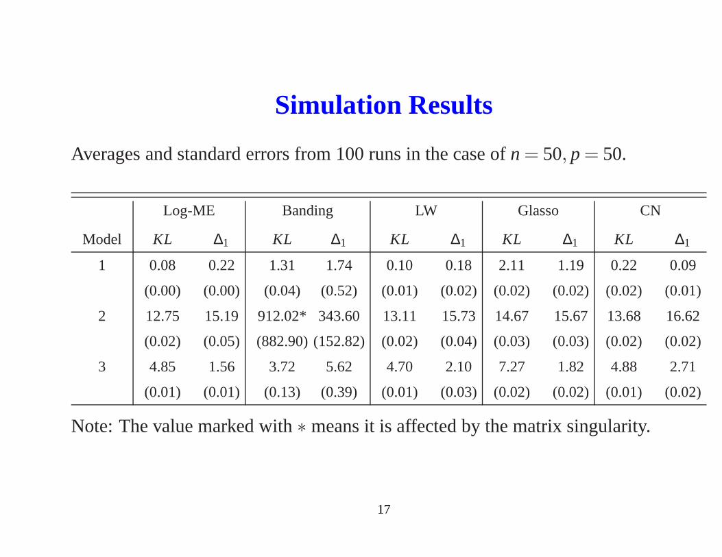
Simulation Results

Averages and standard errors from 100 runs in the case ofn = 50, p = 50.

Log-ME Banding LW Glasso CN

Model KL ∆1 KL ∆1 KL ∆1 KL ∆1 KL ∆1

1 0.08 0.22 1.31 1.74 0.10 0.18 2.11 1.19 0.22 0.09

(0.00) (0.00) (0.04) (0.52) (0.01) (0.02) (0.02) (0.02) (0.02) (0.01)

2 12.75 15.19 912.02* 343.60 13.11 15.73 14.67 15.67 13.68 16.62

(0.02) (0.05) (882.90) (152.82) (0.02) (0.04) (0.03) (0.03) (0.02) (0.02)

3 4.85 1.56 3.72 5.62 4.70 2.10 7.27 1.82 4.88 2.71

(0.01) (0.01) (0.13) (0.39) (0.01) (0.03) (0.02) (0.02) (0.01) (0.02)

Note: The value marked with∗ means it is affected by the matrix singularity.

17

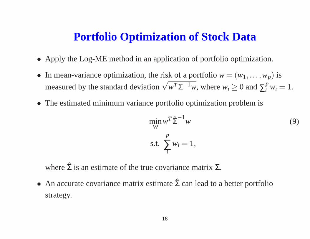
Portfolio Optimization of Stock Data

• Apply the Log-ME method in an application of portfolio optimization.

• In mean-variance optimization, the risk of a portfoliow = (w1, . . . ,wp) is

measured by the standard deviation√

wTΣ−1w, wherewi ≥ 0 and∑pi wi = 1.

• The estimated minimum variance portfolio optimization problem is

minw

wT Σ−1w (9)

s.t.p

∑i

wi = 1,

whereΣ is an estimate of the true covariance matrixΣ.

• An accurate covariance matrix estimateΣ can lead to a better portfolio

strategy.

18

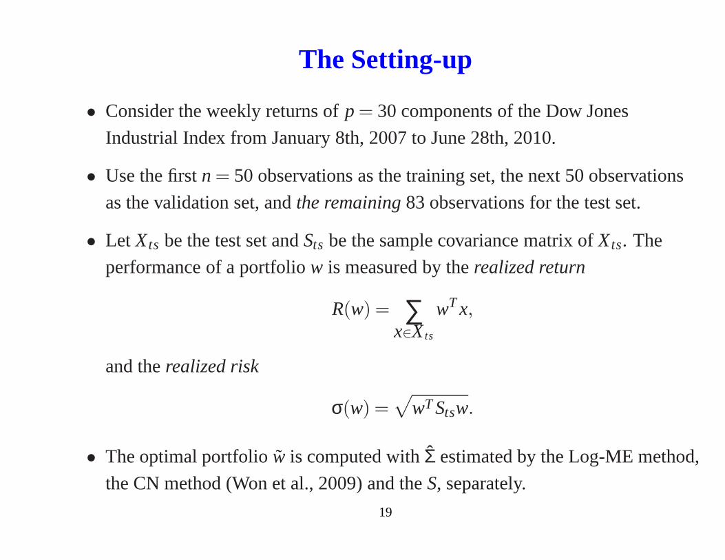
The Setting-up

• Consider the weekly returns ofp = 30 components of the Dow Jones

Industrial Index from January 8th, 2007 to June 28th, 2010.

• Use the firstn = 50 observations as the training set, the next 50 observations

as the validation set, andthe remaining83 observations for the test set.

• Let Xts be the test set andSts be the sample covariance matrix ofXts. The

performance of a portfoliow is measured by therealized return

R(w) = ∑x∈Xts

wTx,

and therealized risk

σ(w) =√

wTStsw.

• The optimal portfoliow is computed withΣ estimated by the Log-ME method,

the CN method (Won et al., 2009) and theS, separately.

19

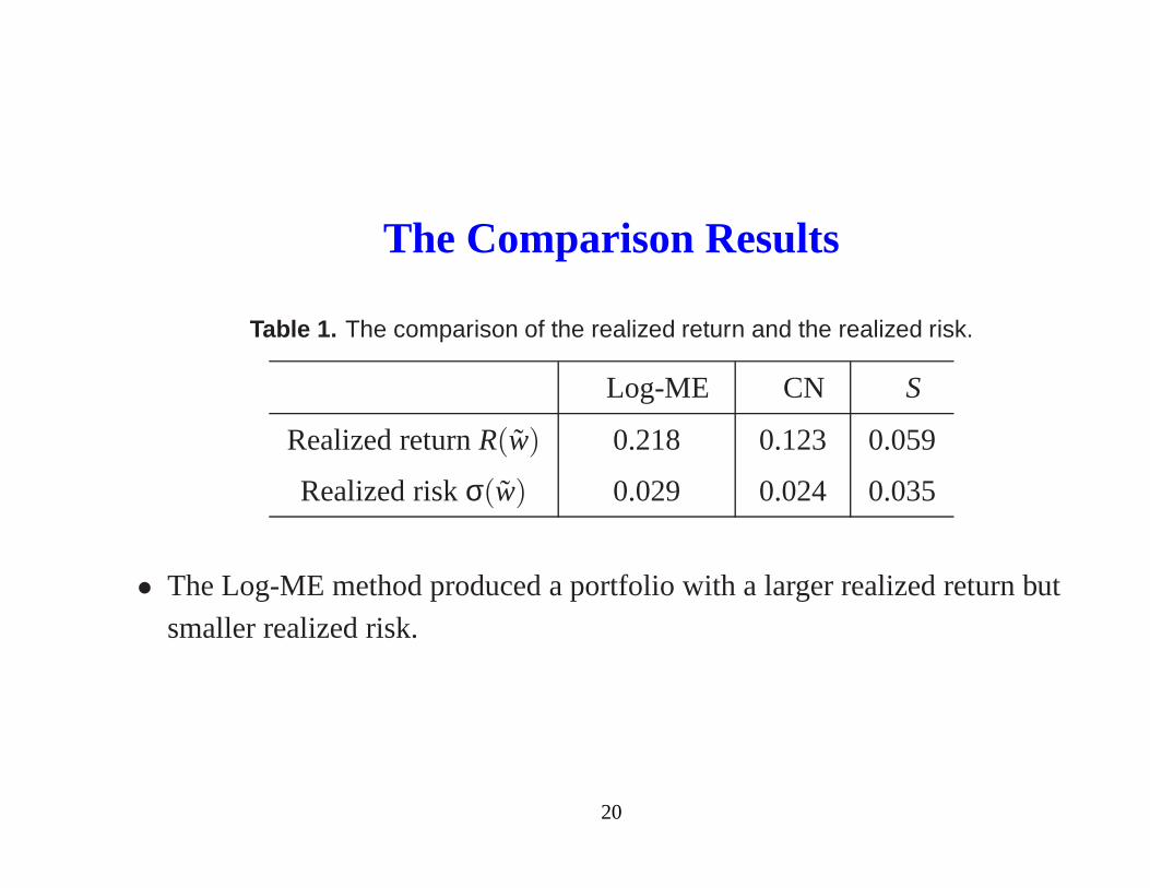
The Comparison Results

Table 1. The comparison of the realized return and the realized risk.

Log-ME CN S

Realized returnR(w) 0.218 0.123 0.059

Realized riskσ(w) 0.029 0.024 0.035

• The Log-ME method produced a portfolio with a larger realized return but

smaller realized risk.

20

Comparison in Different Periods

• Consider the portfolio strategy using the Log-ME method forvarious

covariance matrix estimation methods.

• Given a stating week, use the first 50 observations as the training set, the next

50 observations as a validation set, andthe third50 observationsas a test set.

• Shift the starting week one ahead every time, and evaluate the portfolio

strategy of 33 different consecutive test periods.

• The optimal portfoliow is computed withΣ estimated by the Log-ME method,

the CN method and the sample covariance matrix method, separately.

21

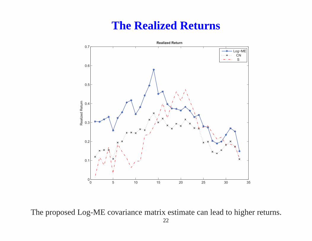
The Realized Returns

0 5 10 15 20 25 30 350

0.1

0.2

0.3

0.4

0.5

0.6

0.7

Realiz

ed R

etu

rn

Realized Return

Log−ME

CN

S

The proposed Log-ME covariance matrix estimate can lead to higher returns.22

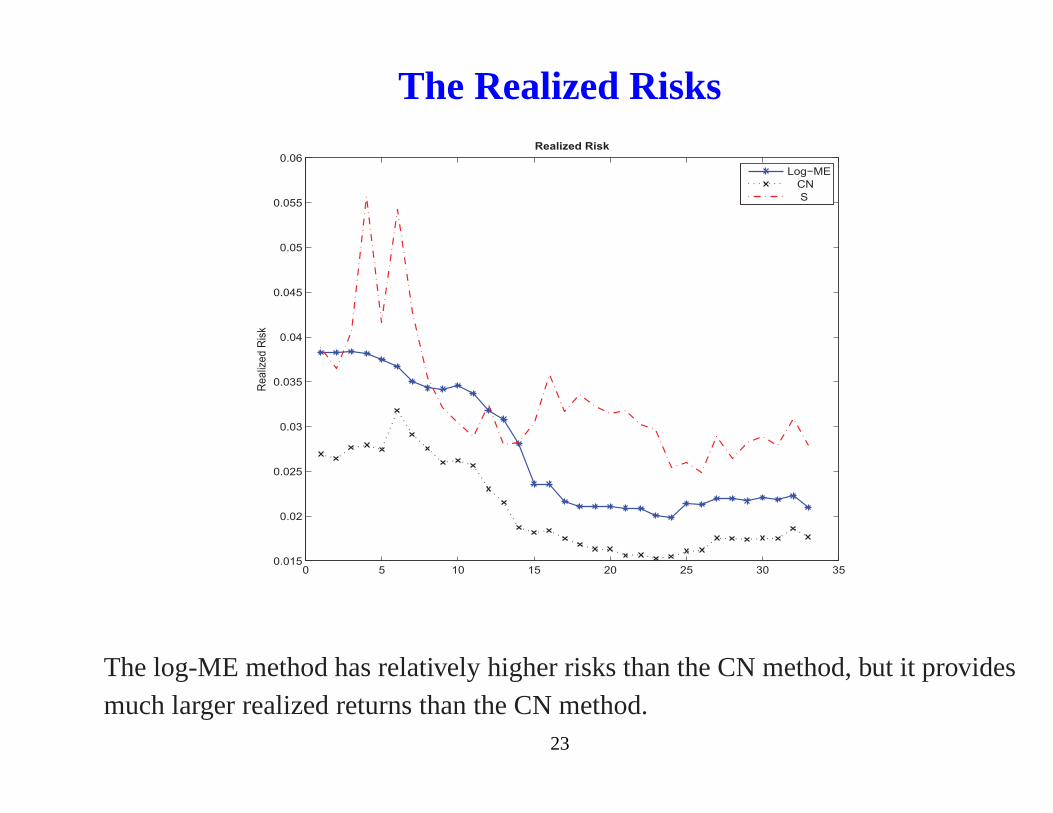
The Realized Risks

0 5 10 15 20 25 30 350.015

0.02

0.025

0.03

0.035

0.04

0.045

0.05

0.055

0.06

Realiz

ed R

isk

Realized Risk

Log−ME

CN

S

The log-ME method has relatively higher risks than the CN method, but it providesmuch larger realized returns than the CN method.

23

Summary

• Estimate the covariance matrix through its matrix logarithm based on a

penalized likelihood function.

• The Log-ME method regularizes the largest and smallest eigenvalues

simultaneously by imposing a convex penalty.

• Other penalty functions can be considered to improve the estimation in

different perspectives.

• Extend to Bayesian covariance matrix estimation for the large-p-small-n

problem.

24

Thank you!

25

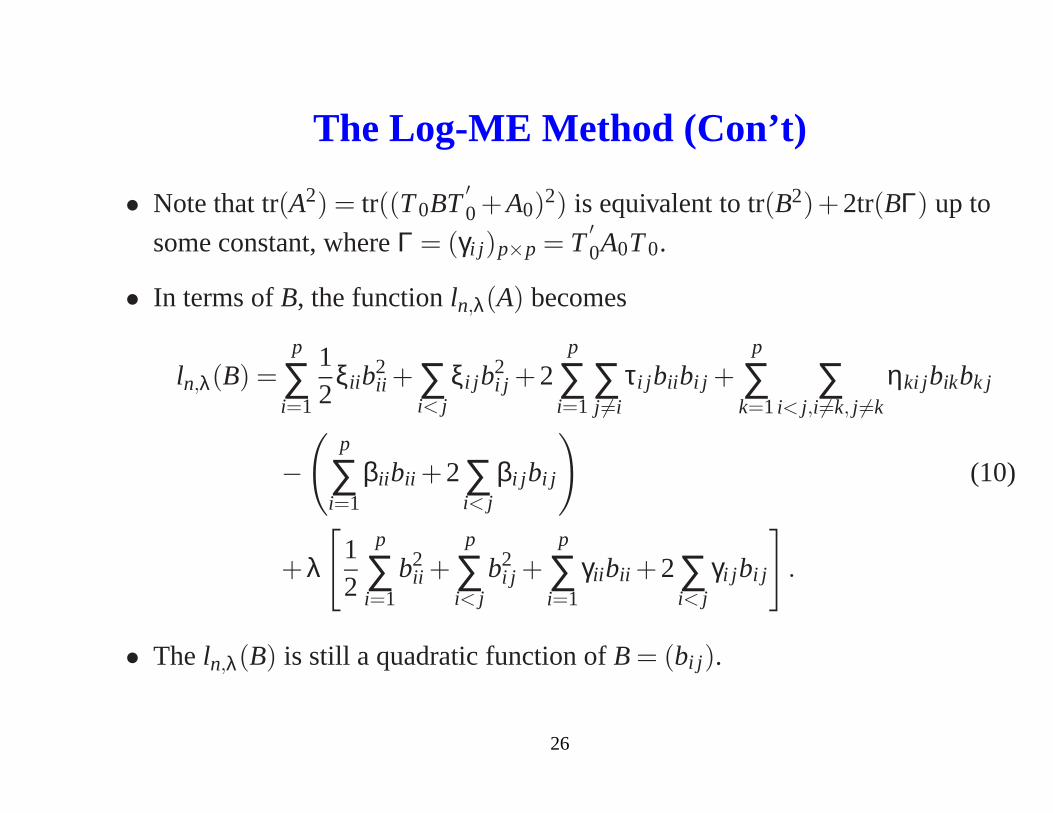
The Log-ME Method (Con’t)

• Note that tr(A2) = tr((T0BT′0 +A0)

2) is equivalent to tr(B2)+2tr(BΓ) up to

some constant, whereΓ = (γi j )p×p = T′0A0T0.

• In terms ofB, the functionln,λ(A) becomes

ln,λ(B) =p

∑i=1

12

ξii b2ii + ∑

i< jξi j b

2i j +2

p

∑i=1

∑j 6=i

τi j bii bi j +p

∑k=1

∑i< j,i6=k, j 6=k

ηki jbikbk j

−(

p

∑i=1

βii bii +2∑i< j

βi j bi j

)

(10)

+λ

[

12

p

∑i=1

b2ii +

p

∑i< j

b2i j +

p

∑i=1

γii bii +2∑i< j

γi j bi j

]

.

• The ln,λ(B) is still a quadratic function ofB = (bi j ).

26

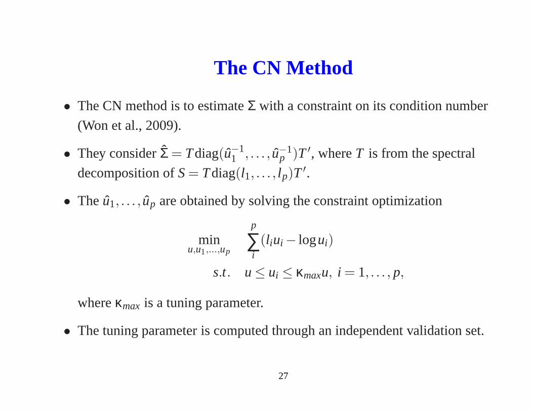
The CN Method

• The CN method is to estimateΣ with a constraint on its condition number

(Won et al., 2009).

• They considerΣ = Tdiag(u−11 , . . . , u−1

p )T ′, whereT is from the spectral

decomposition ofS= Tdiag(l1, . . . , lp)T ′.

• Theu1, . . . , up are obtained by solving the constraint optimization

minu,u1,...,up

p

∑i(l iui − logui)

s.t. u≤ ui ≤ κmaxu, i = 1, . . . , p,

whereκmax is a tuning parameter.

• The tuning parameter is computed through an independent validation set.

27