WORKING PAPER SERIES 03-2017

Πατησίων 76 104 34 Αθήνα Tηλ 210 8203303‐5 Fax 210 8238249

76 Patission Street Athens 104 34 Greece Tel (+30) 210 8203303‐5 Fax (+30) 210 8238249 E‐mail econauebgr wwwauebgr

The driving forces of the current Greek great depression

George Economides Dimitris Papageorgiou

and Apostolis Philippopoulos

1

The driving forces of the current Greek great depression

George Economideslowast Dimitris Papageorgiou and Apostolis Philippopouloslowast

February 12 2017

Abstract This paper provides a quantitative study of the main determinants of the Greek great depression since 2010 We use a medium-scale DSGE model calibrated to the Greek economy between 2000 and 2009 (the euphoria years that followed the adoption of the euro) Then departing from 2010 our simulations show that the fiscal policy mix adopted jointly with the deterioration in institutional quality and specifically in the degree of protection of property rights can explain essentially all the total loss in GDP between 2010 and 2015 (around 26) In particular the fiscal policy mix accounts for 14 of the total output loss while the deterioration in property rights accounts for another 8 It thus naturally follows that a less distorting fiscal policy mix and a stronger protection of property rights are necessary conditions for economic recovery in this country Key words Growth public debt institutions JEL classification numbers O4 H6 E02 Acknowledgements We thank the editors of this volume as well as Harris Dellas Petros Varthalitis Vanghelis Vassilatos and Eva Vourvachaki for discussions and comments We also thank Angelos Kyriazis for excellent research assistantship The second co-author clarifies that the views expressed herein are those of the authors and do not necessarily express the views of the Bank of Greece Any errors are entirely our own Corresponding author George Economides Department of International and European Economic Studies School of Economics Athens University of Economics and Business 76 Patission street Athens 10434 Greece Tel +30-210-8203729 email geconauebgr

lowast Athens University of Economics and Business and CESifo email geconauebgr Economic Analysis and Research Department Bank of Greece email DPapageorgioubankofgreecegr lowast Athens University of Economics and Business and CESifo email aphilauebgr

1

The driving forces of the current Greek great depression

George Economideslowast Dimitris Papageorgiou and Apostolis Philippopouloslowast

February 12 2017

Abstract This paper provides a quantitative study of the main determinants of the Greek great depression since 2010 We use a medium-scale DSGE model calibrated to the Greek economy between 2000 and 2009 (the euphoria years that followed the adoption of the euro) Then departing from 2010 our simulations show that the fiscal policy mix adopted jointly with the deterioration in institutional quality and specifically in the degree of protection of property rights can explain essentially all the total loss in GDP between 2010 and 2015 (around 26) In particular the fiscal policy mix accounts for 14 of the total output loss while the deterioration in property rights accounts for another 8 It thus naturally follows that a less distorting fiscal policy mix and a stronger protection of property rights are necessary conditions for economic recovery in this country Key words Growth public debt institutions JEL classification numbers O4 H6 E02 Acknowledgements We thank the editors of this volume as well as Harris Dellas Petros Varthalitis Vanghelis Vassilatos and Eva Vourvachaki for discussions and comments We also thank Angelos Kyriazis for excellent research assistantship The second co-author clarifies that the views expressed herein are those of the authors and do not necessarily express the views of the Bank of Greece Any errors are entirely our own Corresponding author George Economides Department of International and European Economic Studies School of Economics Athens University of Economics and Business 76 Patission street Athens 10434 Greece Tel +30-210-8203729 email geconauebgr

lowast Athens University of Economics and Business and CESifo email geconauebgr Economic Analysis and Research Department Bank of Greece email DPapageorgioubankofgreecegr lowast Athens University of Economics and Business and CESifo email aphilauebgr

2

1 Introduction

Following the world financial crisis in 2008 most European Union countries have managed to pull

out of recession since 2014 A distinct exception is Greece which has not yet entered a recovery

mode (see European Commission 2016 and CESifo 2016) The Greek economy has been

shrinking since 2009 and Greece has lost around 26 of its GDP over 2010-2015 Thus the

episode seems to satisfy all conditions of a ldquogreat depressionrdquo (see Kehoe and Prescott 2002)1

Actually and making it worse the country is in a multiple crisis public debt is around 177 of

GDP foreign debt is around 142 of GDP unemployment is around 25 and there is still an

environment of political uncertainty and polarization

Despite three bailout packages of around 300 billion euros so far (financed by the European

Union the European Central Bank and the IMF) several structural reforms and the recent

improvement in the international economic environment Greece has not yet shown any sign of real

recovery Paradoxically most of policymakers both in Greece and the EU have been searching for

engines of economic growth without having first studied the determinants of the continuing

depression The present paper tries to fill this gap Identifying the barriers to growth is a prerequisite

for credibly suggesting potential engines of growth2

In particular the aim of the current paper is to decompose the above loss in output into its

main drivers Our main results are as follows Using a medium-scale DSGE model carefully

calibrated to the Greek economy our simulations show that the fiscal policy mix adopted jointly

with developments in institutional quality and specifically in the degree of protection of property

rights can explain around 85 of the total loss in GDP between 2010 and 2015 In particular when

we use the tax-spending mix as it has been in the data since 2010 and we also assume that the

observed deterioration in an index of property rights manifests itself into a decline in total factor

productivity our model can explain around 22 fall in GDP since 2010 (as said the total loss in

the data has been around 26) We also show that the portion due to the fiscal policy mix is 14

while the portion due to the deterioration in property rights is another 8

3

Two clarifications are necessary from the outset The first is about fiscal consolidation Our

results should not be interpreted as saying that most of the Greek crisis is a consequence of fiscal

austerity A kind of fiscal austerity was necessary given the imbalances inherited from the past

once sovereign risk premia emerged in 2010 Greek governments could not choose but undertake

severe fiscal consolidation measures Actually as perhaps should be expected when we simulate

our model under the counter-factual scenario that fiscal policy had remained unchanged as in 2010

the model cannot deliver a dynamically stable solution implying an unsustainable fiscal situation

which in simple words means that the continuation of the status quo was not possible anymore and

that some kind of fiscal stabilization was necessary What our results do hint however is that the

recessionary effects of fiscal stabilization could perhaps have been milder had the policy mix been

different from that actually adopted Greecersquos fiscal stabilization has been based on both spending

cuts and tax rises but the increase in taxes has been particularly high (see subsection 31 below)3

The second clarification is about institutional quality The importance of institutional quality and

especially of property rights for economic growth is well known in the growth literature (see eg

Acemoglu 2009 chapter 4 for a review) It should be stressed that property rights may be affected

by tax policy but they are also affected by the quality of public order and safety where the sharp

deterioration of the latter is clearly documented in the Greek data since 2004 and especially after

2008 (see subsection 32 below) Thus it should not come as a surprise at least qualitatively that

this institutional deterioration is a driver of the Greek depression on the other hand our simulations

show that its quantitative importance for the output loss is striking

The way we work is as follows We employ a medium-scale new-Keynesian DSGE model

of a small open economy enriched with a number of real and nominal frictions so as to capture the

main empirical features of the Greek economy4 The model is calibrated to data up to and including

the year 2009 We take 2009 as the pre-depression benchmark year because the first memorandum

with the Troika (EU ECB and IMF) was agreed in 2010 This first memorandum as well as the

next two in 2012 and 2015 have provided financial assistance and have offered credit to the Greek

4

economy at much more favourable terms than markets would have provided but they have been

ldquoconditioned onrdquo fiscal austerity measures (namely measures to improve debt dynamics) and

structural reforms that have been highly criticized and have led to political polarization and social

unrest Then departing from 2010 and assuming an initial unanticipated shock to public debt as

observed in the data during that year we simulate the effects of the tax-spending mix as it has been

in the actual data during 2010-2015 so as to quantify the portion of the output loss caused by this

particular policy mix In turn we repeat the same exercise by adding the effects of the deterioration

in the property rights index again as it has been in the actual data up to 2015 by assuming that this

deterioration affects the efficiency or productivity with which factor inputs are used (namely it

affects the so-called TFP)5 Quoting Acemoglu (2009 p 105) ldquowhen countries have large drops in

their income due to political instability etc these drops are associated with corresponding declines

in TFPrdquo

A paper close to ours is Gourinchas et al (2016) who also use a micro-founded DSGE

model to analyze the Greek crisis In their paper the crisis is driven by a large menu of shocks

including shocks to default rates banksrsquo funding costs etc We however believe that such variables

can hardly be considered as (extrinsic) shocks Here by contrast we try to identify the primitive

sources of ldquoshocksrdquo6 We show that the particular fiscal policy mix adopted and the deterioration in

institutional quality both as documented in the actual time-series data can explain most of the drop

in output since 2010

The rest of the paper is organized as follows Section 2 introduces the model explains its

calibration and presents the steady state solution Section 3 presents simulations Section 4 closes

the paper

2 A DSGE model

In this section we describe the model used and provide its numerical steady state solution The

latter will serve as a point of departure for the simulations in the next section

5

21 Description of the model

Our quantitative results will be based on a medium-scale DSGE model of a small open economy

calibrated to Greek data The model is a variant of the model used by the Bank of Greece (see

Papageorgiou 2014) We choose to work with this particular model because it is used by an official

institution like the Bank of Greece and also because it is relatively detailed and hence can capture

the main features of the Greek macro economy

The model exhibits a number of real and nominal frictions so as to capture the key features

of the Greek economy and thus provide a parameterized general equilibrium model suitable for

policy simulations These frictions include imperfectly competitive labor and product markets the

distinction between Ricardian and non-Ricardian households real wage rigidity Calvo-type short-

term nominal fixities habit persistence various adjustment costs a variety of firms so as to capture

tradable and non-tradable goods a relatively rich public sector including the production of public

goodsservices by the use of public employees loss of monetary policy independence since Greece

is part of the euro zone and also an imperfect world capital market where the interest rate at which

domestic agents borrow from the world capital market rises with public debt

The building blocks of the model and its final equilibrium system are presented in detail in

the Appendix (see Appendix A) The final equilibrium system consists of 89 equations in 89

endogenous variables This is given the exogenously set policy instruments initial conditions for

the state variables and total factor productivity (TFP) in the two sectors tradables and non-

tradables

22 Numerical solution of the model

The above model is calibrated to data from the Greek economy This means that (most of) its

parameter values match average data values and that the exogenously set policy instruments are set

as in the data The data source is Eurostat unless otherwise stated The data are at annual frequency

and cover the period 2000-2015 although the period used for this calibration stage is up to and

6

including 2009 (as explained in the Introduction we use pre-crisis euro period data)7 Table A1 in

the Appendix reports the calibrated parameter values and the average values of fiscal policy

variables in the data

Using these numerical values the system is then solved using a Newton-type non-linear

method as implemented in DYNARE (see below for specification of transition dynamics) Its steady

state solution (at least for the key variables) is reported in Table 1 In this solution we have

exogenously set the debt-to-GDP ratio equal to the threshold level 126d equiv which was the value

of the public debt-to-GDP in 2009 (that was the year that risk premia emerged in Greece) so that

one of the remaining fiscal policy instruments needs to be determined residually to satisfy the

within period government budget constraint we assume that it is lump-sum taxes that play this role

As Table 1 shows the solution is in line with data averages over 2000-2009 and can thus provide a

reasonable departure point for the changes that have been taking place since 2010 and are described

in the next sections In particular the solution does a relatively good job at mimicking the position

of the country (and its different sectors) in the international capital market as well as the

consumption-investment behavior of the private sector over the euro pre-crisis years

Table 1 Steady state solution and data averages 2000-09

Variable data solution Total private consumption-to-GDP 065 059

Private investment-to-GDP 018 017 Total work hours 026 026

Work hours in private sector 022 022

Total public debt-to-GDP 126 126 Lump-sum taxestransfers - 0045

Economyrsquos net foreign liabilities-to-GDP 077 066

Private net foreign liabilities-to-GDP 003 0 Exports-to-GDP 023 027

Total imports-to-GDP 034 024

Note (i) Average data over the euro period 2000-2009 with the exception of foreign liabilities which are over the period 2003-2009 and the public debt-to-GDP ratio which is set at its 2009 data value The data source is Eurostat and the Bank of Greece (ii) A positive value of the net foreign liabilities-to-GDP ratio means that the domestic country is a net borrower

7

3 Simulations

As said above departing from the ldquosteady staterdquo solution in Table 2 we will now simulate the

above economy when fiscal policy and institutional quality change as observed in the data after

2010 To understand how the model works we will start by assuming that only fiscal policy has

changed and then we will add changes in institutional quality That is we study one dynamic driver

at a time

31 Effects of the fiscal austerity mix as adopted in practice

In this subsection we will examine other things equal the impact of fiscal consolidation policies as

adopted in Greece since 2010

We work as follows We assume that in 2010 there was an initial shockincrease in the

public debt-to-GDP ratio by 20 pp (as observed in the data) We then set all exogenous fiscal (tax-

spending) instruments as they have actually been in the data during 2010-15 (to isolate the impact

of actual fiscal policy we switch-off the extra feedback reaction to public debt during this sub-

period) Besides in order to mimic the memorandum package we set the interest rate at which the

government borrows from abroad as a weighted average of the risk-free world interest rate and the

world interest rate that the economy would face if it had to borrow from the international capital

market (the latter includes the country risk-premium as in the data)8 The private sector on the other

hand continues to face the full world interest rate (that includes the country risk-premium) when it

borrows from the international market Recall that this premium is a function of the public debt gap

where in this gap the public debt threshold above which premia emerge is 126

We will assume that all the above features continue until the year 2015 (this is the year that

this paper is being written in terms of data availability) Then after 2015 the fiscal instruments are

assumed to gradually return to their pre-crisis 2009 values In particular we assume that they follow

an autoregressive process using as initial values the 2015 values and an autoregressive coefficient

equal to 09 We allow one fiscal instrument to react to the public debt gap (see equation 27) where

8

in this gap the public debt target in the policy rules is the pre-shock value of 126 The interest

rate at which the government borrows from abroad is now allowed to react fully to the degree of

governmentrsquos indebtedness

Thus in our first simulations transition dynamics is driven by the above changes in fiscal

policy We solve the model under perfect foresight (as said above we use a Newton-type non-linear

method as implemented in DYNARE)

The simulated impulse response functions are plotted in Figure 1 while Table 2 summarizes

the associated changes in the main macro variables vis-agrave-vis their values in the data Inspection of

the simulated results in the third column of Table 2 and comparison to the actual data in the second

column implies that the GDP decreases by around 14 between 2009 and 2015 In the data the

actual decrease has been 26 during the same time interval That is the particular fiscal austerity

package which has been adopted between 2010 and 2015 can account for more than half of the big

fall in output observed in the data during this period

Figure 1 Impulse response functions driven by the fiscal austerity package

Note All variables are expressed as percentage deviations from the steady-state with the exception of the CPI inflation the interest rate foreign assets and the public debt-to-GDP ratio that are expressed as percentage point deviations

Year2010 2020 2030 2040

D

evia

tion

-15

-10

-5

0Real Output

Year2010 2020 2030 2040

D

evia

tion

-5

0

5

10Domestic Tradable Output

Year2010 2020 2030 2040

D

evia

tion

-30

-20

-10

0Non-Tradable Output

Year2010 2020 2030 2040

D

evia

tion

-30

-20

-10

0

10Consumption

TotalRicardianNon-Ricardian

Year2010 2020 2030 2040

D

evia

tion

-30

-20

-10

0

10Private Investment

Year2010 2020 2030 2040

D

evia

tion

-6

-4

-2

0Real Wages-Private Sector

2010 2020 2030 2040

P

oint

Dev

iatio

n

-2

-1

0

1CPI Inflation

Year2010 2012 2014 2016 2018

P

oint

Dev

iatio

n

0

1

2

3Interest Rate

Year2010 2020 2030 2040

D

evia

tion

-5

0

5

10Real Exchange Rate

Year2010 2020 2030 2040

D

evia

tion

-20

-10

0

10Trade Volumes

Exports

Imports

Year2010 2020 2030 2040

P

oint

Dev

iatio

n

-6

-4

-2

0

2Foreign Assets

Year2010 2020 2030 2040

P

oint

Dev

iatio

n

-40

-20

0

20

40Public Debt GDP

9

Table 2 Changes in the main macro variables 2015-2009 ()

Variable Data Simulated model with the fiscal package

Simulated model with the fiscal package plus

institutional shocks

Real GDP -26 -137 -22

Real private

consumption

-277 -46 -91

Real private investment -60 -191 -406

Real exchange rate 8 28 -25

Real exports 182 26 -6

Note (i) The changes in the actual time series are computed as log deviations between their 2015 and 2009 values with the exception of real private investment that is computed as 2015 2009 2009( ) I I Iminus The data source is Eurostat Changes in

the simulated series correspond to log deviations from the initial steady state (ii) A positive change for the real effective exchange rate means a real depreciation ie an improvement in the countryrsquos competitiveness

Figure 2 depicts the dynamic paths of fiscal policy instruments under this scenario It thus

confirms the well-recognized feature that the Greek fiscal consolidation program has been based on

both spending cuts and tax rises (see eg European Commission 2015) although the clear rise in all

effective tax rates is particularly striking for a country suffering from a deep recession

Figure 2 Dynamic paths of fiscal policy instruments

Note Government intermediate consumption investment and the public sector wage bill are expressed as shares of the 2009 GDP The effective tax rates are computed following the approach in Papageorgiou et al (2012) The data source is Eurostat

Year2010 2015 2020 2025 2030 2035

007

008

009

01

Government Intermediate Consumption GDP

Year2010 2015 2020 2025 2030 2035

003

004

005

Government Investment GDP

Year2010 2015 2020 2025 2030 2035

01

011

012

013Government Wages GDP

Year2010 2015 2020 2025 2030 2035

017

018

019

02

021Government Transfers GDP

Year2010 2015 2020 2025 2030 2035

016

017

018

019Tax Rate on Consumption

Year2010 2015 2020 2025 2030 2035

036

038

04

Tax Rate on Labour

Year2010 2015 2020 2025 2030 2035

02

022

024

026

Tax Rate on Capital

Year2010 2015 2020 2025 2030 2035

0

002

004

Lump-Sum Taxes

10

Finally we close by reporting that the model would be dynamically unstable (meaning that

there is no solution) if we had assumed that the independently set fiscal policy instruments

remained as they were in the pre-2010 period In other words as said in the Introduction the fiscal

situation was not sustainable and hence some kind of fiscal policy adjustment was unavoidable in

the aftermath of the 2008 world crisis

32 Effects of the deterioration in institutional quality

We will now add another driver of transition dynamics namely changes in institutional quality and

in particular an index that measures the protection of property rights

As said in the Introduction we assume that developments in this index manifest themselves

as shocks to TFP This is a short cut and is similar to the methodology of Chari et al (2007) In

other words as a short cut we construct an ldquoeffectiverdquo TFP series where the degree of

effectiveness is shaped by changes in the degree of property rights protection On the other hand it

should be stressed that it is straightforward to enrich our model so as in the presence of weak

property rights atomistic agents find it to optimal to allocate effort to conflict and extraction and

in equilibrium this leads to resource misallocation that eventually reduces the effective TFP in

Appendix B we provide a simple version of our full-fledged DSGE model that shows this

equivalence formally9 Chari et al (2007) also work with a prototype economy with wedges or

adverse shocks and then show that micro-founded frictions in a more detailed economy manifest

themselves as such wedges or adverse shocks in the prototype economy

We therefore proceed as follows First we construct a series of institutional quality Then

using this we will construct a corresponding series for the effective TFP and finally will feed this

resulting TFP series into our theoretical model in section 2 That is now the modelrsquos dynamics will

be driven both by the fiscal austerity package and the effective TFP series

To construct a measure of the quality of institutions that protect property rights we use the

World Bankrsquos ldquoWorldwide Governance Indicatorsrdquo dataset which has been widely used in many

11

empirical studies (see eg Akitoby and Stratmann (2008) and Baldacci et al (2011)) The

institutional quality index is the sum of the following three indicators ldquorule of lawrdquo ldquoregulatory

qualityrdquo and ldquopolitical stability and absence of violenceterrorismrdquo These indicators are all closely

related to issues concerning the protection of property rights10 Figure 3 shows the evolution of this

composite index over the period 2002-2015 Notice the remarkable decline of institutional quality

after 2008 which was a year of intense social and political turmoil in Greece It should be stressed

that these indicators are not linked (at least directly) to public finances

Figure 3 Deterioration in property rights in Greece (2002-2015)

Note The index is computed as the sum of the following three indicators ldquorule of lawrdquo ldquoregulatory qualityrdquo and ldquopolitical stability and absence of violenceterrorismrdquo The data source is Worldwide Governance Indicators World DataBank

In turn as said above we assume that changes in the TFP level are ldquoshapedrdquo by changes in

the above index of institutional quality In the model there are two specific TFP levels namely in

the tradable and the non-tradable sector We allocate the changes over time in this index to the

respective TFPs according to the relative size of the tradable and non-tradable sectors in the data

(the ratio of the gross value added in the tradable sector to the non-tradable sector is 08) Thus we

obtain time series for the TFP levels in the two sectors and we normalize them so that their values

Year2002 2004 2006 2008 2010 2012 2014

06

08

1

12

14

16

18

2

22

24

12

in 2009 to be consistent with the calibrated values of the TFPs (equal to 1 for the non-tradable and

equal to 09241 for the tradable sector) Figure 4 shows the two constructed effective TFP series

Figure 4 TFP in tradable and non-tradable sectors

ldquoshapedrdquo by the deterioration in property rights

Note The path of the TFP levels is ldquoshapedrdquo by the changes in the institutional quality index according to the relative size of the respective sectors in the data Source Authorsrsquo calculations

Finally using all the above we repeat the same experiment as in section 31 by setting the

TFP levels of tradables and non-tradables over 2010-2015 equal to the constructed series The new

impulse response functions are plotted in Figure 5 while the last column in Table 2 which was

presented above summarizes the associated changes in the main macro variables Notice that now

the reduction in GDP in column 3 of Table 2 is 22 as compared to only 14 without the

TFPinstitutional shock in column 2

Year2009 2010 2011 2012 2013 2014 2015

085

09

095

1

105

TFP Tradable Sector

TFP Non-Tradable Sector

13

Figure 5 Impulse response functions driven by the fiscal austerity package and the deterioration in property rights

Note All variables are expressed as percentage deviations from the steady-state with the exception of the CPI inflation the interest rate foreign assets and the public debt-to-GDP ratio that are expressed as percentage point deviations

4 Conclusions discussion and extensions

In this paper we studied the quantitative importance of the fiscal austerity program and the

deterioration of institutional quality both as observed in the recent data for the Greek great

depression since 2010 The main result is that the adopted fiscal policy mix and the deterioration in

property rights are the main explanatory variables of the Greek great depression

We close with acknowledging two caveats First here we did not explain why the specific

fiscal policy mix has been chosen (which proves to be particularly distorting) or why the society has

chosen to have weak and deteriorating property rights (which leads to misallocation of resources

and hence to a relatively low TFP) In general it is well recognized that the policies chosen andor

the way resources are (mis)allocated are an equilibrium outcome of a political process interacting

with institutions and distribution (see eg Acemoglu (2009 chapter 4) and Jones (2011)) In the

case of Greece there is no shortage of conjectures about the root causes of such choices which go

back to the post-world war II history of the country Second our analysis here was only positive

One could search for instance for alternative fiscal policy mixes andor institutional regimes that

could perhaps mitigate the recessionary effects of debt consolidation We leave these extensions for

future research

Year2010 2020 2030 2040

D

evia

tion

-30

-20

-10

0Real Output

Year2010 2020 2030 2040

D

evia

tion

-15

-10

-5

0

5Domestic Tradable Output

Year2010 2020 2030 2040

D

evia

tion

-40

-30

-20

-10

0Non-Tradable Output

Year2010 2020 2030 2040

D

evia

tion

-60

-40

-20

0Consumption

TotalRicardianNon-Ricardian

Year2010 2020 2030 2040

D

evia

tion

-60

-40

-20

0

20Private Investment

Year2010 2020 2030 2040

D

evia

tion

-30

-20

-10

0Real Wages-Private Sector

2010 2020 2030 2040

P

oint

Dev

iatio

n

-2

0

2

4CPI Inflation

Year2010 2012 2014 2016 2018

P

oint

Dev

iatio

n

0

1

2

3Interest Rate

Year2010 2020 2030 2040

D

evia

tion

-10

-5

0

5Real Exchange Rate

Year2010 2020 2030 2040

D

evia

tion

-20

-10

0

10Trade Volumes

Exports

Imports

Year2010 2020 2030 2040

P

oint

Dev

iatio

n

-4

-2

0

2Foreign Assets

Year2010 2020 2030 2040

P

oint

Dev

iatio

n

-40

-20

0

20

40Public Debt GDP

14

References

Acemoglu D (2009) Modern Economic Growth Princeton University Press Princeton Anderson D Hunt B amp Snudden S (2014) Fiscal consolidation in the euro area How much pain can structural reforms ease Journal of Policy Modeling 36 785-799 Ardagna S (2001) Fiscal policy composition public debt and economic activity Public Choice 109 301-325 Akitoby B amp Stratmann T (2008) Fiscal policy and financial markets Economic Journal 118 1971-1985 Angelopoulos K Philippopoulos A amp Vassilatos V (2009) The social cost of rent seeking in Europe European Journal of Political Economy 25 280-299 Baldacci E Petrova I Belhocine N Dobrescu G amp Mazraani S (2011) Assessing fiscal stress IMF Working Papers WP11100 Washigton DC Bergoeing R Kehoe P Kehoe T and Soto R (2002) Policy driven productivity in Chile and Mexico in the 1980s and 1990s American Economic Review 92 16-21 Blanchard O amp Gali J (2007) Real wage rigidities and the new Keynesian model Journal of Money Credit and Banking 39 35-65 Cacciatore M Duval R amp Fiori G (2012) Short-term gain or pain A DSGE model based analysis of the short-term effects of structural reforms in labour and product markets OECD Economics Department Working Papers no 948 OECD Paris Calvo GA (1983) Staggered prices in a utility-maximizing framework Journal of Monetary Economics 12 383-398 Canova F (2007) Methods for Applied Macroeconomic Research Princeton University Press Princeton CESifo (2016) EEAG Report on the European Economy Munich Chari VV Kehoe P amp McGrattan E (2007) Business cycle accounting Econometrica 75 781-836 Christoffel K Coenen G amp Warne A (2008) The new area-wide model of the Euro area ndash A micro-founded open-economy model for forecasting and policy analysis European Central Bank Working Paper Series Number 944 Christoffel K amp Linzert T (2010) The role of real wage rigidities and labor market frictions for unemployment and inflation dynamics Journal of Money Credit and Banking 42 1435-1446 Christiano LJ amp Eichenbaum M (1992) Current real business cycle theories and aggregate labor market fluctuations American Economic Review 82 430-450 Christiano LJ Eichenbaum M amp Evans C (2005) Nominal rigidities and the dynamic effects of a shock to monetary policy Journal of Political Economy 113 1-45

15

Christiano LJ Trabandt M amp Walentin K (2011) DSGE models for monetary policy analysis In Friedman BM Woodford M (Eds) Handbook of Macroeconomics Volume 3 Elsevier North-Holland 285ndash367 Coenen G Mohr M amp Straub R (2008) Fiscal consolidation in the euro area long run benefits and short-run costs Economic Modeling 25 912-932 Coenen G Straub R amp Trabandt M (2013) Gauging the effects of fiscal stimulus packages in the euro area Journal of Economic Dynamics and Control 32 367-386 Corsetti G Kuester K Meier A amp Muller G (2013) Sovereign risk fiscal policy and macroeconomic stability Economic Journal 123 F99-F132 Duval R (2008) Is there a role for macroeconomic policy in fostering structural reforms Panel evidence for OECD countries over the past two decades European Journal of Political Economy 24 491-502 Economides G Park H amp Philippopoulos A (2007) Optimal protection of property rights in a general equilibrium model of growth Scandinavian Journal of Economics 109 153-175 Economides G Kalyvitis S amp Philippopoulos A (2008) Does foreign aid distort incentives and hurt growth Theory and evidence from 75 aid-recipient countries Public Choice 134 463-488 Economides G Papageorgiou D Philippopoulos A amp Vassilatos V (2013) Smaller public sectors in the Euro Area Aggregate and distributional implications CESifo Economic Studies 59 536-558 Eggertsson G Ferrero A amp Raffo A (2014) Can Structural reforms help Europe Journal of Monetary Economics 61 2-22 Erceg JC amp Linde J (2013) Fiscal consolidation in a currency union Spending cuts vs tax hikes Journal of Economic Dynamics and Control 37 422-445 European Commission (2010) The economic adjustment programme for Greece European Economy Occasional Papers Number 61 Brussels European Commission (2014) Public Finances in EMU Brussels European Commission (2015) Public Finances in EMU Brussels Forni L Monteforte L amp Sessa L (2009) The general equilibrium effects of fiscal policy estimates for the euro area Journal of Public Economics 93 559-585 Forni L Gerali A amp Pisani M (2010a) The macroeconomics of fiscal consolidations in euro area countries Journal of Economic Dynamics and Control 34 1791-1812 Forni L Gerali A amp Pisani M (2010b) Macroeconomic effects of greater competition in the service sector The case of Italy Macroeconomic Dynamics 14 677-708 Forni L amp Pissani M (2013) Macroeconomic effects of sovereign restructuring in a Monetary Union A model-based approach IMF Working Paper Number 13269

16

Gali J Lopez-Salido D amp Valles J (2007) Understanding the effects of government spending on consumption Journal of the European Economic Association 5 227-270 Garcia-Cicco J Pancrazi R amp Uribe M (2010) Real Business Cycles in Emerging Countries American Economic Review 100 2510-2531 Gerali A Notarpietro A and Pisani M (2014) Macroeconomic effects of simultaneous implementation of reforms after the crisis Bank of Italy Working Paper Number 997 Gerali A Notarpietro A amp Pisani M (2015) Structural reforms investment and zero lower bound in a monetary union Manchester School 83 120-139 Gogos S Mylonidis N Papageorgiou D amp Vassilatos V (2014) 1979-2001 A Greek great depression through the lens of neoclassical growth theory Economic Modelling 36 316-331 Gomes S Jacquinot P Mohr M amp Pisani M (2013) Structural reforms and macroeconomic performance in the euro area countries A model-based assessment International Finance 16 23- 44 Gourinchas P-O Philippon T amp Vayanos D (2016) The analytics of the Greek crisis Mimeo London School of Economics Hall R (2003) Wage determination and employment fluctuations NBER Working Paper Number 9967 Hall R (2005) Employment fluctuations with equilibrium wage stickiness American Economic Review 95 50-64 Heylen F Hoebeeck A amp Buyse T (2013) Government efficiency institutions and the effects of fiscal consolidation on public debt European Journal of Political Economy 31 40-59 IMF (2015a) Euro area policies 2015 Article IV consultation Country Report Number 15204 International Monetary Fund Washington IMF (2015b) Fiscal monitor - Now is the time Fiscal policies for sustainable growth International Monetary Fund Washington Jones C (2008) Macroeconomics Norton and Company New York Jones C (2011) Misallocation economic growth and input-output economics NBER Working Paper Number 16742 Kaufmann D Kraay A amp Mastruzzi M (2010) The worldwide government indicators Methodology and analytical issues World Bank Policy Research Working Papers Number 5430 Kehoe T amp Prescott E (2002) Great depressions of the 20th century Review of Economic Dynamics 5 1-18 Kliem M amp Uhlig H (2013) Bayesian estimation of a DSGE model with asset prices Deutsche Bundesbank Discussion Paper Number 372013

17

Malley J Philippopoulos A amp Woitek U (2009) To react or not Fiscal policy volatility and welfare in the EU-3 European Economic Review 53 689ndash714 Mendoza E (2010) Sudden stops financial crises and leverage American Economic Review 100 1941-1966 Mertens K amp Ravn M (2011) Understanding the aggregate effects of anticipated and unanticipated policy shocks Review of Economic Dynamics 14 27ndash54 OECD (2013) Economic Policy Reforms Going for Growth Paris OECD (2015) Economic Policy Reforms Going for growth Paris Papageorgiou D Efthimiadis T amp Konstantakopoulou I (2012) Effective tax rates in Greece Centre of Planning and Economic Research (KEPE) Discussion Paper Series Number 124 Papageorgiou D (2012) Fiscal policy reforms in general equilibrium the case of Greece Journal of Macroeconomics 34 504-522 Papageorgiou D (2014) BoGGEM A dynamic stochastic general equilibrium model for policy simulations Bank of Greece Working Paper Number 182 Papageorgiou D amp Vourvachaki E (2016) Macroeconomic effects of structural reforms and fiscal consolidations Trade-offs and complementarities European Journal of Political Economy Available from httpdxdoiorg101016jejpoleco201608010 Petrongolo B amp Pissarides C (2001) Looking into the black box A survey of the matching function Journal of Economic Literature 38 390-431 Philippopoulos A Vassilatos V and Varthalitis P (2016) Fiscal consolidation in an open economy with sovereign premia and without monetary policy independence International Journal of Central Banking forthcoming Prescott E (2002) Prosperity and depression American Economic Review 92 1-15 Roeger W amp in lsquot Veld J (2013) Expected sovereign defaults and fiscal consolidations European Economy Economic Papers no 479 Schmitt-Groheacute S amp Uribe M (2003) Closing small open economies Journal of International Economics 61 163-185 Schuknecht L von Hagen J amp Wolswijk G (2009) Government risk premiums in the bond market EMU and Canada European Journal of Political Economy 25 371-384 Stahler N amp Thomas C (2012) Fimod ndash A DSGE model for fiscal policy simulations Economic Modelling 29 239-261 Uhlig H (2007) Explaining asset prices with external habits and wage rigidities in a DSGE model American Economic Review 97 239-243 Vogel L (2012) Structural reforms fiscal consolidation and external rebalancing in monetary union A model-based analysis Economic Modelling 29 1286-1298

18

Vogel L (2014a) Nontradable sector reform and external rebalancing in monetary union A model-based analysis Economic Modelling 29 1286-1298 Vogel L (2014b) Structural reforms at the zero bound European Economy Economic Papers no 537

19

1 Namely the drop in output is large occurred rapidly and is sustained this is defined as a ldquogreat depressionrdquo See Gogos et al (2014) for an application of this methodology to the Greek economy before the euro period 2 There is a growing literature on the current Greek crisis For instance Bortz (2015) discusses where the financial assistance has gone offering a different view from that of Sinn (2015) Arellano and Bai (2016) study the Greek default Papageorgiou and Vourvachaki (2016) study the implications of structural reforms in light of the crisis Gourinchas et al (2016) search for shocks that can account for the Greek crisis See below for further details 3 See eg Philippopoulos et al (2016) for the different implications of different fiscal policy mixes used for debt consolidation in Italy 4 Alternatively we could for instance use a VAR approach which requires a limited amount of theory to structure the data (see eg Canova 2007 for methodology) We prefer to follow the DSGE approach so as to have well-defined micro-foundations that allow us to understand the behavioral channels through which exogenous changes affect macroeconomic outcomes 5 There is a large literature that shows how weak institutions affect the efficiency with which factor inputs are used and in particular how weak property rights lead to distortive individual incentives resource misallocation and eventually a lower level of total factor productivity See eg Jones (2008 chapter 4 and 2011) and Acemoglu (2009 chapter 4) for reviews of the literature while see below for further details and references Here working as in Chari et al (2007) we will take a short cut by assuming that changes in property rights directly show up as shocks to TFP nevertheless as argued in subsection 32 below this is equivalent to a richer model where the adverse effect of weak property rights on TFP works via the distortion of individual incentives 6 See eg Chari et al (2007) for a methodology paper on business cycle accounting 7 We focus on the period during which Greece is part of the euro area but before the debt crisis erupted in early 2010 8 In particular we assume that ( ) 1G H

t t tR mR m R= + minus where we set the value of m equal to 05

9 In the same spirit Economides et al (2007 2008) and Angelopoulos et al (2009 2012) also provide micro-founded dynamic general equilibrium models where the presence of weak property rights distorts private incentives and in equilibrium this leads to resource misallocation which in turn maps into reductions in the effective TFP All this belongs to a rich and still growing literature that endogenizes the TFP and hence endogenizes long-term growth 10 The rule of law indicator captures perceptions of the extent to which agents have confidence in and abide by the rules of society and in particular the quality of contract enforcement property rights the police and the courts as well as the likelihood of crime and violence The regulatory quality index captures perceptions of the ability of the government to formulate and implement sound policies and regulations and the credibility of governmentrsquos commitment to such policies The political stability and absence of violenceterrorism indicator captures perceptions of the likelihood that the government will be destabilized or overthrown by unconstitutional or violence means including politically-motivate violence and terrorism For further details see Kaufman et al (2010) We report that each one of these three sub-indexes is highly correlated with key macroeconomic variables such as real GDP and real investment in the Greek data

20

Appendix A A DSGE model and calibration

This appendix presents the model used It is similar to that in Papageorgiou (2014)

1 Households

The economy is populated by a continuum of households of mass one indexed by [ ]01hisin of

which a fraction indexed by [01 ]i λisin minus are referred as ldquoRicardianrdquo or ldquooptimizing householdsrdquo

and a fraction indexed by (1 1]j λisin minus are referred as ldquonon-Ricardianrdquo or ldquoliquidity constrained

householdsrdquo Optimizing households have access to capital and financial markets where they can

invest in the form of physical capital government bonds and internationally traded assets Liquidity

constrained households on the other hand are not able to lend or borrow so that they consume

their disposable labor income in each time period Both households supply differentiated labor

services and act as wage-setters in monopolistically competitive markets

11 Ricardian households

Ricardian households indexed by i have preferences over consumption and leisure The inter-

temporal utility function of each i is

( )10 0

Rt cti i t i t

tU E u C C Hβ ξ

infin

minus

=

= minussum (1)

where (01)β isin is the discount factor i tC is i rsquos effective consumption (defined below) at t i tH is

i rsquos total work hours at t [01)cξ isin is a parameter that measures the degree of external habit

formation in consumption and 1RtC minus denotes average (per household i ) lagged-once effective

consumption Effective consumption is in turn defined to be a linear combination of private

consumption p

i tC and public goods and services (education health etc) provided by the state

sector gtY 1

p g

i t i t tC C Yϑ= + (2)

where [ 11]ϑisin minus is the degree of substitutability between private and public consumption

The instantaneous utility function is assumed to be of the form

( ) ( )1

1 1 log

1

R R i tc ct ti t i t i t

Hu C C H C C

g

ξ ξ κg

+

minus minusminus = minus minus+

(3)

1 See eg Christiano and Eichenbaum (1992) Forni et al (2010a) and Economides et al (2013)

21

where g is the inverse of Frisch labour supply elasticity and 0κ gt is a preference parameter

related to work effort Each household i supplies work hours in the private sector p

i tH and the

public sector gi tH As in eg Ardagna (2001) and Forni et al (2009) hours of work can be moved

across the two sectors and are perfect substitutes in terms of (dis)utility so that p g

i t i t i tH H H= + in

each period t

The Ricardian household can save in the form of physical capital p

i tI domestic government

bonds i tB and foreign assets p

i tF It receives labour income from working in the private sector

p p

i t i tw H and the public sector g gi t i tw H where

pi tw and

gi tw are the real wage rates in the private and

public sector respectively The household rents out capital to firms and receives capital income

k p

t i t i tr u K where ktr is the real return to the effective amount of private capital

pi tK is the physical

private capital stock and 0i tu gt is the utilization rate of capital The household also earns interest

income from domestic government bonds and internationally traded assets that pay a gross nominal

interest 1tR ge and 1HtR ge at 1t + respectively In addition households own all domestic firms so

that they receive their profits as dividends i tDiv Finally each Ricardian household receives a

lump-sum government transfer tri tG The household pays taxes on consumption 0 1c

ttlt lt on

labour income 0 1lttlt lt on capital earnings and dividends 0 1k

ttlt lt and lump-sum taxes tT

Hence the budget constraint of each Ricardian household i is

( )

( )( ) ( )( )

1 1

1

1

1 1

pIi t t i tc p pt

t i t i tC C Ct t t

l p p g g k k pt i t i t i t i t t t i t i t i t

t

B S FPC IP P P

w H w H r u K Div

R

t

t t

+ +

minus

+ + + + =

= minus + + minus + +

+ 1

pi t t i tH tr h

t i t t i tC Ct t

B S FR G T

P Pminus+ + minus minusG

(4)

where CtP and I

tP are the prices of a unit of the private consumption final good and the investment

final good respectively and tS is the nominal exchange rate (expressed in terms of domestic

currency per unit of foreign currency) The household faces costs when it adjusts its private foreign

asset holdings hi tG whenever the private foreign assets-to-GDP ratio GDP

tY

t

ptit

YPFS 1 + deviates from its

long-run target level f In particular

( )2

1 1

2

pY GDPft i th p Y GDP C t t

i t t i t t t t C Y GDPt t t

S FP YS F P Y P fP P Y

ξ ++

G = minus

(5)

22

where GDPtY is the economyrsquos real GDP Y

tP is the GDP deflator and 0gefξ is an adjustment cost

parameter2

The private capital stock evolves over time according to the following law of motion

( )( ) 1

1

1 1p

i tp p p I pi t i t i t i tp

i t

IK u K I

Iδ+

minus

= minus + minusΨ

(6)

where IΨ is a convex adjustment cost function for investment as in eg Christiano et al (2005)

2

1 1

12

p pki t i tIp p

i t i t

I II I

ξ

minus minus

Ψ = minus

(7)

where (1) (1) 0I IΨ = Ψ = and 0kξ ge is an adjustment cost parameter We assume that the

depreciation rate of private capital depends on the rate of capacity utilization and is a convex

function that satisfies 0pδ prime gt 0pδ primeprime gt so that ( ) p p

i t i tu uϕδ δ= where (01)pδ isin and 0ϕ gt are

respectively the average rate of depreciation of private capital and the elasticity of marginal

depreciation cost

The first-order conditions of this problem are written below when we present the final

equilibrium system

12 Non-Ricardian households

Liquidity constrained households indexed by j have the same preferences as Ricardian

households They receive labour income from working in the private and public sectors but have no

access to capital or financial markets so that in each period their consumption spending equals

their after-tax wage income plus lump-sum government transfers The period-by-period budget

constraint of each household j is

( ) ( )( ) 1 1c l p p g g trt j t t j t j t j t j t j tC w H w H Gt t+ = minus + + (8)

where pj tH and

gj tH are respectively hours worked in the private and public sector by household j

and trj tG is a lump-sum government transfer to each j Thus as in eg Coenen et al (2013) we

allow for a potentially uneven distribution of government transfers across Ricardian and non-

Ricardian households

The first-order conditions of this problem are written below when we present the final

equilibrium system

2 This specification ensures that foreign private assets are stationary see eg Schmitt-Grohe and Uribe (2003)

23

2 Wage setting and the evolution of wages in the private sector

We assume that wages in the private sector are set by monopolistic unions as in eg Forni et al

(2009) and Gali et al (2007) More specifically households supply differentiated labour varieties to

a continuum of unions [ ]01hisin each of which represents a specific labour variety Every variety is

uniformly distributed across households so that each union ultimately represents 1 λminus fraction of

Ricardian households and λ of non-Ricardian households In every period each union sets the

wage rate for its own workers by trading off the utility derived from private sector labour income

and the disutility of total work effort by taking into account the demand for the differentiated labour

variety h At the same time private and public sector firms allocate their labour demand uniformly

across the h labour varieties independently of the type of households which implies that hours

worked by each type of household are equal

h p h p pj t i t h tH H H= equiv and

h g h g gj t i t h tH H H= equiv 3

Therefore in each period a typical union h chooses the wage rate ph tw to maximize

( ) ( ) ( )1

1 1 1

1h tNR l p p R l p p

w h t h t h t h t h t h t

HL w H w H

g

λ t λ t κg

+

= L minus + minus L minus minus + (9a)

subject to

1

Wt

Wt

ph tp p

h t tpt

wH H

w

micromicro

minusminus

=

(9b)

p g

h t h t h tH H H= + (9c)

where Eq (9b) is the demand for the differentiated labour input h ptH is total labour demand in the

private sector ptw is the aggregate wage rate in the private sector and

NRh tL

Rh tL are the marginal

utilities of consumption of non-Ricardian and Ricardian households of labour variety h

respectively used as weights Finally ( ) 1 1W Wt tmicro micro minus gt is the elasticity of substitution across the

differentiated labour services where 1Wtmicro gt is the wage markup in the private labour market

Focusing on a symmetric equilibrium in which all unions choose the same wage rate ex

post the first-order condition of the above problem is

1p Wt tNR R

t t

wMRS MRS

λ λ micro minus

+ =

(10)

3 Total public sector labour demand for the differentiated labour input ℎ is exogenous and is defined as 1

0

g gt h tH H dh= int

24

where ptw is the optimal wage rate chosen by unions and NR

tMRS and RtMRS are the marginal

rates of substitution between consumption and leisure of non-Ricardian and Ricardian households

respectively4

Following eg Hall (2005) and Blanchard and Gali (2007) we introduce further rigidities in

the labour market by assuming that real wages respond sluggishly to labour market conditions In

particular the real wage rate in the private sector is modeled as a weighted average of the lagged-

once real wage rate and the optimal real wage rate chosen by unions

( ) ( )11

n np p pt t tw w w

minus

minus= (11)

where 0 1nle le denotes the degree of real wage rigidities and ptw is given by (10)5 This

formulation aims to capture the rigidities found in the Greek labour market (see eg the discussion

in European Commission 2010)6

3 Production in the private sector

There are two types of domestic firms The first type consists of monopolistically competitive firms

that produce intermediate goods tradable and non-tradable The continuum of firms producing

differentiated varieties of tradables indexed by [ ]01Tf isin sell their output domestically or abroad

(the latter are recorded as exports) The continuum of firms producing differentiated varieties of

non-tradables indexed by [ ]01Nf isin sell their output domestically only There is also a continuum

of monopolistically competitive firms importing intermediate goods indexed by [ ]01Mf isin The

second type of firms consists of four perfectly competitive firms that produce final goods These

firms combine purchases of intermediate goods to produce four non-tradable goods a private

consumption good a private investment good a public consumption good and a public investment

good Finally there is a foreign final goods firm that combines purchases of the exported domestic

intermediate goods

4 Note that when 0λ = ie when all households are Ricardian W

tmicro reduces to a markup of the optimally chosen real

wage rate over the marginal rate of substitution between consumption and leisure of Ricardian households 5 See also eg Uhlig (2007) Malley et al (2009) and Kliem and Uhlig (2013) for a similar specification Microfoundations for Eq (11) can be found in eg Hall (2003) Petrongolo and Pissarides (2001) and Christoffel and Linzert (2010) 6 Papageorgiou (2014) finds that this specification can capture rather well the aggregate dynamics of work hours and real wages in Greece

25

31 Final goods firms

As said above there are four representative final goods firms that combine purchases of tradable

intermediate goods with non-tradable goods to produce a private consumption good ptC a private

investment good ItI a public consumption good gc

tG and a public investment good gitG

Private consumption goods producer

The representative producer of the private final consumption good combines a bundle of tradable

consumption intermediate goods TtC with a bundle of non-tradable intermediate goods N

tC

according to a constant elasticity of substitution (CES) production function

( ) ( )1 11 1 1

(1 )

C

C C CC CC C

p T Nt C t C tC C C

εε ε ε

ε εε εω ωminus minus minus

= + minus

(12)

where [ ]01Cω isin measures the weight of tradable goods in the production of the final private

consumption good and 0Cε gt is the elasticity of substitution between tradable and non-tradable

consumption goods

In turn the tradable intermediate consumption good bundle is a CES function of the

domestically produced bundle of tradable intermediate consumption goods DtC and the bundle of

imported intermediate consumption goods MtC

( ) ( )1 11 1 1

(1 )

TC

TC TC TCTC TCTC TC

T D Mt TC t TC tC C C

εε ε ε

ε εε εω ωminus minus minus

= + minus

(13)

where [ ]10isinTCω measures the home bias in the production of the tradable intermediate

consumption good and 0TCε gt is the elasticity of substitution between domestic and imported

intermediate consumption goods

The intermediate consumption good bundles that are used as inputs combine differentiated

varieties supplied by intermediate good firms Specifically the varieties supplied by each tradable

intermediate goods firm Tf T

Df t

C each non-tradable intermediate-goods firm Nf N

Nf t

C and each

importing firm Mf M

Mf t

C are respectively combined using a CES technology into

( )1

1

0

Tt

Tt

TD D Tt f t

C C dfmicro

micro

= int (14a)

26

( )1

1

0

Nt

Nt

NN N Nt f t

C C dfmicro

micro

= int (14b)

( )1

1

0

Mt

Mt

MM M Mt f t

C C dfmicro

micro

= int (14c)

where 1T N Mt t tmicro micro micro gt are the intra-temporal elasticities of substitution between different varieties

within each type of intermediate consumption good As we show below T N Mt t tmicro micro micro represent

markups in the markets of domestic and imported intermediate goods

Given the above technology the producer of the final private consumption good solves a

three stage problem In the first stage it takes as given the prices of domestic tradable N

Df t

P non-

tradable T

Nf t

P and imported intermediate goods M

Mf t

P and chooses the amounts of the

differentiated goods T

Df t

C N

Nf t

C M

Mf t

C in order to minimize total expenditures for the bundles of

the differentiated goods 1

0

T TD D Tf t f t

P C dfint 1

0

N NN N Nf t f t

P C dfint 1

0

M MM M Mf t f t

P C dfint subject to the aggregation

constraints in (14a)-(14c) The solution of the cost minimization problem gives the demand

functions for these intermediate goods Tf Nf and Mf respectively

1

Dt

DtT

T

Df tD D

tDf tt

PC C

P

micromicro

minusminus

=

(15a)

1

Nt

NtN

N

Nf tN N

tNf tt

PC C

P

micromicro

minusminus

=

(15b)

1

Mt

MtM

T

Mf tM M

tMf tt

PC C

P

micromicro

minusminus

=

(15c)

where D N Mt t tP P P are the aggregate price indices of domestic tradable non-tradable and imported

intermediate consumption goods respectively

In the second stage the firm chooses the bundles DtC and M

tC in order to maximize its

profits 1C TC T D D M Mt t t t t t tP C P C P CP = minus minus subject to the technology constraint (13) and by taking as

given the price indexes of domestic tradables TCtP non-tradables D

tP and imported intermediate

consumption goods MtP Thus it solves

27

max

D Mt t

TC T D D M Mt t t t t t

C CP C P C P Cminus minus

subject to

( ) ( )1 11 1 1

(1 )

TC

TC TC TCTC TCTC TC

T D Mt TC t TC tC C C

εε ε ε

ε εε εω ωminus minus minus

= + minus

In the third stage the firm chooses the demand for TtC and N

tC to maximize profits

2C C C TC T N Nt t t t t t tP C P C P CP = minus minus subject to the technology constraint (12) and by taking the input

prices CtP TC

tP and NtP as given Thus it solves

max

T Nt t

C C TC T N Nt t t t t t

C CP C P C P Cminus minus

subject to

( ) ( )1 11 1 1

(1 )

C

C C CC CC C

p T Nt C t C tC C C

εε ε ε

ε εε εω ωminus minus minus

= + minus

The demand functions for domestic tradable and imported consumption goods as well as for

tradable and non-tradable intermediate consumption goods resulting from the optimization problem

of the final consumption good firm are

TCD Dt t

TCT TCt t

C PC P

ε

ωminus

=

(16a)

( )1TCM M

t tTCT TC

t t

C PC P

ε

ωminus

= minus

(16b)

CT TCt t

CC Ct t

C PC P

ε

ωminus

=

(16c)

( )1CN N

t tCC C

t t

C PC P

ε

ωminus

= minus

(16d)

From the zero profit condition we get the price index for tradable consumption goods

( ) ( )( )1

1 1 11TC TC TCTC D M

t TC t TC tP P Pε ε εω ω

minus minus minus = + minus and the price index of a unit of the final consumption

good (ie the Consumption Price Index) ( ) ( ) ( )1

1 1 11C C CC TC N

t C t C tP P Pε ε εω ω

minus minus minus = + minus where

D N Mt t tP P P are the prices of domestic tradable intermediates non-tradable intermediates and

imported intermediate goods respectively

28

Private investment goods producer

Optimal decisions regarding the production of the final private investment good are derived in an

analogous manner as above The representative producer of the private investment good combines a

composite bundle of tradable intermediate goods TtI with a bundle of non-tradable intermediate

goods NtI to generate a composite final private investment good I

tI by using a constant elasticity

of substitution (CES) production function

( ) ( )1 11 1 1

(1 )

I

I I II II I

I T Nt I t I tI I I

εε ε ε

ε εε εω ωminus minus minus

= + minus

where [ ]01Iω isin measures the weight of tradable goods in the production of the final private

investment good and 0Iε gt is the elasticity of substitution between tradable and non-tradable

investment goods

In turn the composite bundle of the tradable intermediate investment good that is used in the

production of final investment goods is a CES function of domestically produced tradable

intermediate investment goods DtI and imported intermediate investment goods M

tI

( ) ( )1 1 11 1

(1 )

TI

TITI TITI TITI TI

T D Mt TI t TI tI I I

εεε ε

ε εε εω ωminusminus minus

= + minus

where [ ]01TIω isin measures the home bias in the production of the tradable intermediate

consumption good and 0TIε gt is the elasticity of substitution between domestic and imported

investment goods

The demand functions for domestic tradable and imported investment goods as well as for

tradable and non-tradable investment goods are

TID Dt t

TIT TIt t

I PI P

ε

ωminus

=

( )1TIM M

t tTIT TI

t t

I PI P

ε

ωminus

= minus

IT TIt t

II It t

I PI P

ε

ωminus

=

( )1IN N

t tIT I

t t

I PI P

ε

ωminus

= minus

29

where ( ) ( )( )1

1 1 11TI TI TITI D M

t TI t TI tP P Pε ε εω ω

minus minus minus = + minus and ( ) ( )( )

11 1 11

I I II TI Nt I t I tP P P

ε ε εω ωminus minus minus = + minus

are respectively the price indices for tradable intermediate investment goods and final investment

goods

Public consumption and investment goods production

Regarding the final public consumption and investment goods gctG and gi

tG we assume they are

produced using only non-tradable intermediate goods Hence gc Nt tG GC= and gi N

t tG GI= where

( )1

1

0

Nt

Nt

NN N Nt f t

GC GC dfmicro

micro

= int and ( )

11

0

Nt

Nt

NN N Nt f t

GI GI dfmicro

micro

= int

The optimal demand functions are

1

Nt

NtN

N

Nf tN N

tNf tt

PGC GC

P

micromicro

minusminus

=

and 1

Nt

NtN

N

Nf tN N

tNf tt

PGI GI

P

micromicro

minusminus

=

Aggregating across final good producing firms we get the respective aggregate domestic demand

functions for non-tradable domestic tradable and imported intermediate goods Tf Nf and mf

1

Nt

NtN

N N N N N

Nf tNT N N N N NT

tNf t f t f t f t f tt

PY C I GC GI Y

P

micromicro

minusminus

= + + + =

1

Tt

TtT

T T T

Df tD D D D

tDf t f t f tt

PY C I Y

P

micromicro

minusminus

= + =

1

Mt

MtM

M M M

mf tM M M M

tmf t f t f tt

PY C I Y

P

micromicro

minusminus

= + =

where NT N N N Nt t t t tY C I GC GI= + + + D D D

t t tY C I= + and M M Mt t tY C I= + are respectively the total

demand for non-tradable goods total domestic demand for domestically produced tradable goods

and total demand for imports

32 Intermediate goods firms

Each tradable and non-tradable intermediate good Tf t

Y and Nf t

Y is produced by a continuum of

monopolistically competitive intermediate goods firms indexed by [ ]01Tf isin and [ ]01Nf isin

respectively according to the production technologies

30

( ) ( ) ( )1

T T G

T T T

a a aT gt t Tf t f t f t

Y A K H Kminus

= minusΦ (17a)

( ) ( ) ( )1

N N G

N N N

a a aN gt t Nf t f t f t

Y A K H Kminus

= minusΦ (17b)

where Tf t

K is private capital Tf t

H is work hours in the private sector gtK is public capital

0T Na a gt are the output elasticities of capital services in the tradable and non-tradable sectors

respectively and 0Ga gt is the output elasticity of public capital7 Finally 0T NΦ Φ ge are fixed

costs of production and TtA N

tA are sector-specific total factor productivity levels

Tradable sector

In what follows we present the problem of intermediate goods firms in the tradable sector

Domestic intermediate goods firms in the tradable sector solve a two-stage problem In the first

stage each firm takes as given factor prices ktr and p

tw and chooses capital and labour inputs

Tf tK and

Tf tH in order to minimize total real input cost We also introduce a working capital

channel in the form of a ldquocash-in-advancerdquo constraint in the spirit of eg Mendoza (2010) In

particular at the beginning of each period each firm borrows from international lenders in order to

cover a fraction (01)tv isin of their total labour costs in advance of revenuesrsquo receipt The working

capital loan is repaid by the end of the period at the domestic country gross interest rate HtR Thus

the intratemporal problem of each firm involves the minimization of their costs inclusive of the

costs of serving their intra-period working capital loan In other words

( )

min 1T T TT Tf t f t

k p H pt t t t tf t f t f tK H

r K w H R v w H+ + minus (18)

subject to (17a)

The first-order conditions are

( )( ) ( )

1 1 1T

T

T

Tf tH pt t t T f t

f t

YR w a mc

Hν

+Φ+ minus = minus (19)

T

T

T

Tf tkt T f t

f t

Yr a mc

H

+Φ= (20)

where Tf t

mc is the Lagrange multiplier associated with the technology constraint that is the real

marginal cost in terms of the consumer prices CtP Because firms borrow to cover part of their

7 These production functions have increasing returns to scale with respect to all inputs and constant returns to scale with respect to private inputs (see also eg Baxter and King (1993) and Leeper et al (2010))

31

labour costs the marginal cost of labour is higher than the wage rate in the private sector As a

result increases in either the share of labour costs that are financed through working capital loans

or in the domestic interest rate directly increase the cost of labour and thereby reduce labour

demand

The labour input Tf t

H is a composite aggregate of household-specific varieties T

hf t

H

( )1

1

0

Wt

Wt

T Th

f t f tH H

micro

micro

= int Optimal demand is

1

Wt

T T

ph thpf t f t

t

wH H

w

micro =

where ( 1) 1W Wt tmicro micro minus gt is the

elasticity of substitution across differentiated labour services and ptw is the aggregate real wage

index in the private sector that is given by ( )11

1 10

Wt

Wtp p

t h tw wmicro

micro

minus

minus

= int

In the second stage intermediate good firms in the tradable sector choose the price that

maximizes discounted real profits As in Christoffel et al (2008) firms charge different prices at

home and abroad setting prices in producer currency In both domestic and foreign markets we

assume that prices are sticky aacute la Calvo (1983) In particular each period t the firm Tf optimally

resets prices with a constant probability 1 Dpθminus when it sells its differentiated product in the

domestic market and with probability 1 Xpθminus when it sells its product abroad The firms that cannot

optimize partially index their prices to aggregate past inflation according to the price indexation

schemes ( )1 1

D

T T

xD D Dtf t f t

P P minusminus= P and ( )1 1

X

T T

xX X Xtf t f t

P P minusminus= P where

TDf t

P denote the domestic price of

good Tf T

Xf t

P its foreign price and 1D D Dt t tP PminusP = 1X X X

t t tP PminusP = where D Xt tP P are the

aggregate domestic and export price indices (defined below) respectively The indexation

parameters [ ] 01D Xx x isin determine the weights given to past inflation

Each firm Tf which can optimally reset its price in period t knows with probability Dpθ

that this price will continue to be in effect t periods ahead and so chooses the optimal price

TD

f tP

to maximize the discounted sum of expected real profits (in terms of consumer prices CtP ) by

taking aggregate domestic demand DtY and the aggregate price index in the domestic market D

tP

as given Thus each firm Tf maximizes

( ) ( )

1

0 1

maxTD

TDTf t

DR Dx f tD D D Dt tt p t s tR D Df tP st t t

P PE mc YP P

t tt t

t tt t t

βθinfin

+ ++ minus + +

= = + +

L P minus L sum prod (21)

32

subject to

( )1

1

1

Tt

TtTD

T

Dx f tD D D

t s tDf ts t

PY Y

P

t

t

micromicrot

tt

+

+

minusminus

+ minus += +

= P prod (22)

where D C T Dt t t tmc P mc P= is the real marginal cost in terms of the domestic price index and

R Rt tt+L L is the ratio of the marginal utilities of consumption of Ricardian households - that are the

owners of the firms - according to which firms value future profits8 Notice that since all firms face

the same marginal cost and take aggregate variables as given any firm that optimizes will set the

same price

TD D

tf tP P=

Thus the first-order condition of the above problem is

( ) ( ) ( )1

1 1

1 1

0

Tt

TD Dtx xD DR D D D

t s t sD D T Dt t t tt p t t tR D D D D D

s st t s t t t s t

P P PE Y mcP P P

t

t

micromicro

t tt t tt t t

t

βθ micro

+

+

minusminus

+ minus + minus+ ++ + +

= =+ + +

P PL minus = L P P

prod prod (23)

According to the above expression firms set nominal prices so as to equate the average future

expected marginal revenues to average future expected marginal costs9 The aggregate domestic

index evolves according to ( )( ) ( )( )111

1 11 11

Tt

TDT ttxD D D D D D

t p t p t tP P Pmicro

micromicroθ θ

minus

minusminusminus minus

= minus + P

Similarly the associated first-order condition of each firm Tf that chooses its price in the

foreign market in period t is

( ) ( ) ( )1

1 1

1 1

0

Xt

XX Xtx xX XR X X X

t s t sX X X Xt t t tt p t t tR X X C X X

s st t s t t t s t

P P PE Y mcP P P

t

t

micromicro

t tt t tt t t

t

βθ micro

+

+

minusminus

+ minus + minus+ ++ + +

= =+ + +

P PL minus = L P P

prod prod (24)

where X C T Xt t t tmc P mc P= is the real marginal cost in terms of the aggregate export price index and

the aggregate export price index is ( )( ) ( )( )111

1 11 11

Xt

XXx ttxX X X X X X

t p t p t tP P Pmicro

micromicroθ θ

minus

minusminusminus minus

= minus + P

8 In equilibrium the marginal utility of consumption is common across Ricardian households

Ri t tL = L

9 In the case of fully flexible prices 0Dpθ = the above condition reduces to the static relation D T C T

t t t tP P mct tmicro + +=

which states that the price is equal to a markup over the nominal marginal cost

33

Non-tradable sector

The optimal demand by each firm Nf for labour of type h is

1

Wt

Wt

N N

ph thpf t f t

t

wH H

w

micromicro

minusminus

=

and the

aggregate demand for labour of type h is

11

0

Wt

Wt

N

ph tN h N

h t tpf tt

wH H df H

w

micromicro

minusminus

= =

int where NtH is total

labour demand in the non-tradable intermediate good sector As in the case of the tradable good

firms non-tradable intermediate good firms take short-term loans from international lenders at the

home countryrsquos gross interest rate HtR in order to finance a fraction tv of their total labour costs

To minimize costs each firm takes as given the factor prices ktr and p

tw and chooses N Nf t f t

K H

in order to minimize total real input cost ( ) 1N N N

k p H pt t t t tf t f t f t

r K w H R v w H+ + minus subject to the

production function The first-order conditions are

( )( ) ( )

1 1 1N

N

N

Nf tH pt t t N f t

f t

Yv R w a mc

H

+Φ+ minus = minus

N

N

N

Tf tkt N f t

f t

Yr a mc

K+Φ

=

where due to symmetry N

Ntf t

mc mc=

Non-tradable intermediate good firms face price stickiness aacute la Calvo with 1 Npθminus being the

probability that a firm Nf can optimally reset its price in any given period 0t ge The optimal

pricing is characterized by the following conditions

( ) ( ) ( )1

1 1

1 1

0

Nt

Nd Ntx xN NR N N N

t s t sN N N Nt t t tt p t t tR N N C N N

s st t s t t t s t

P P PE Y mcP P P

t

t

micromicro

t tt t tt t t

t

βθ micro

+

+

minusminus

+ minus + minus+ ++ + +

= =+ + +

P PL minus = L P P

prod prod

and the aggregate domestic index evolves according to

( )( ) ( )( )111

1 11 11

Nt

NNN ttxN N N N N N

t p t p t tP P Pmicro

micromicroθ θ

minus

minusminusminus minus

= minus + P

Importing firms

There is a continuum of importing firms [ ]01Mf isin each of which imports a single differentiated

intermediate good M

Mf t

Y These firms operate under monopolistic competition so that they have

34

pricing power This creates a wedge between the price at which the importing firms buy the foreign

differentiated goods in the world markets Yt tS P and the price at which they sell these goods to

domestic households M

Mf t

P Importing firms face price stickiness aacute la Calvo with 1 Mpθminus being the

probability that a firm Mf can optimally reset its price in the domestic market in any given period

0t ge so that optimal pricing follows

( ) ( ) ( )1

1 1

1 1

0

Mt

Mm mtx xM MR M M M

t s t sm M M Mt t t tt p t t tR M M C M M

s st t s t t t s t

P P PE Y mcP P P

t

t

micromicro

t tt t tt t t

t

βθ micro

+

+

minusminus

+ minus + minus+ ++ + +

= =+ + +

P PL minus = L P P

prod prod

and the aggregate import price index evolves according to

( )( ) ( )( )111

1 11 11

Mt

MmM ttxM m M m M M

t p t p t tP P Pmicro

micromicroθ θ

minus

minusminusminus minus

= minus + P

33 Demand from foreign final goods firms

We now model the demand coming from foreign firms or equivalently specify the domestic

countryrsquos exports Recall that the domestic economy produces intermediate tradable goods that are

also exported and so we need to model a final goods firm that transforms them into final goods

There is a representative foreign final good firm that purchases the differentiated exported goods

X

f tY produced by the domestic tradable intermediate good firms Tf and transforms them into a

homogeneous final good XtY via the CES technology

( )1

11

0

XtX

tT

X X Tt f t

Y Y dfmicro

micro

= int (25)

where 1Xtmicro gt is related to the intratemporal elasticity of substitution between the differentiated

outputs supplied by domestic intermediate good firms ( ) 1 1X Xt tmicro micro minus gt

The foreign firm takes the prices of exported differentiated goods

TX

tf tP S (expressed in

terms of the foreign currency) as given and chooses the optimal amounts of differentiated inputs to

minimize total input costs ( )1

0T T

X X Ttf t f t

P S Y dfint subject to (25) so that the optimal demand function

for each input T

Xf t

Y is 1

Xt

XtT

T

Xf tX X

tXf tt

PY Y

P

micromicro

minusminus

=

where ( )11

11

0

Xt

Xt

TX X T

t f tP P df

micro

micro

minus

minus

= int is the aggregate

price index of exported domestic intermediate goods and XtY is total foreign demand for domestic

35

intermediate goods The latter is

XX

X t tt tX

t

P SY YP

εminus

=

where X

tP is the price of foreign

competitors in the export markets tY is foreign economy output and 0Xε gt is the price elasticity

of export demand

4 The public sector

We now model the public sector

41 Government budget constraint and fiscal policy instruments

The government levies taxes on consumption labour income capital earnings and dividends We

also assume lump-sum taxestransfers The government also sells one-period government bonds to

the domestic bond market 1gtB + and the international market 1

gtF + Total tax revenues plus the issue

of new government bonds are used to finance government consumption ctG investment i

tG

transfers trtG and the wage bill of public sector employees g g

t tw H Moreover the interest rates

that the government pays on inherited domestic public debt and on foreign public debt are tR and

GtR respectively We assume that G

tR is a weighted average of the market interest rate that the

country faces when it borrows from abroad and the risk-free world interest rate (see below for

details) Thus the within-period government budget constraint in per-capita terms is

( ) ( )1 1

1 1

g gc p l p p g g k k pt t tt t t t t t t t t t t t tc C

t tN N g g

c i tr g g Gt t t t tt t t t t t tC C C C

t t t t

B S F C w H w H r u K Div TP P

P P B S FG G G w H R RP P P P

t t t+ +

minus minus

+ + + + + + + =

= + + + + +

(26)

Therefore the government has eleven policy instruments 1 1 c l k g g c i tr g gt t t t t t t t t t t tX T w H G G G B Ft t t + +isin

out of which ten can be exogenously set

To ensure dynamic stability we need to assume that one of the exogenously set fiscal policy

instruments follows a state-contingent rule reacting systematically to deviations of the public debt-

to-GDP ratio from a target level and the rate of change of debt

( ) ( )1 1 2 1d y d y y

t t t t tX X D d D Dφ φminus minus= + minus + minus (27)

where 1 1

y tt y GDP

t t

DDP Yminus minus

equiv denotes the debt-to-GDP ratio in the beginning of period t d is a target value

of the public debt-to-GDP ratio (see below for details) and 1 2 0d dφ φ gt are feedback policy reaction

coefficients (as in a Taylor rule for the nominal interest rate)

36

For notational convenience we will define the share of total public debt held by domestic

agents at the end of period t as 1

1

gt

tt

BD

ζ +

+

equiv where 0 1tζle le so that 1 1(1 )gt t t tS F Dζ+ += minus and

1 1 1g g

t t t tD B S F+ + += +

42 Production of public goodsservices

On the production side following eg Forni et al (2010a) and Economides et al (2013 2016) we

assume that the government combines public spending on goods and services ctG and public

employment gtH to produce public goodsservices g

tY according to the production function

( ) ( )1g c gt t t tY A G H

c cminus= (28)

where 0 1cle le is a technology parameter

The law of motion of public capital in per-capita terms is

( )1 1g g g it t tK K Gδ+ = minus + (29)

where ( )01gδ isin is the depreciation rate of public capital stock and 0 0gK gt is given

Regarding the inputs used in the above production function ctG is produced by final good

firms that use only non-tradable intermediate goods as inputs (see above) while gtH is total public

sector demand for the differentiated labour variety h that is exogenous (see above)

5 World capital markets and sovereign spreads

Following most of the literature on small open economies we assume that when domestic

households and the government participate in the world capital market they face an interest rate

that is public debt elastic (see eg Schmitt-Grohe and Uribe 2003)

In particular the nominal interest rate at which the country borrows from the international

market HtR bears a risk-premium term 0tψ ge that introduces a wedge between the interest rate

that the home country faces and the risk-free world nominal interest rate tR

max Ht t t tR R Rψ= + (30)

where as in eg Christiano et al (2011) Garcia-Cicco et al (2010) and Philippopoulos et al

(2016) the risk-premium is assumed to be an increasing function of public debt imbalances

( )( )1exp 1d yt tD dψ ψ += minus minus (31)

where 0dψ ge is a risk parameter and 0d gt is an exogenous threshold above which premia

emerge Thus when the public debt-to-GDP ratio is above a threshold level an interest rate spread

37

arises which is consistent with empirical evidence (see eg Ardagna et al 2008 Roeger and inrsquot

Veld 2013 Schuknecht et al 2009 Corsetti et al 2013) Conceptually the risk premium

component on the right hand side of (31) reflects the risk of sovereign or country default and thus

provides a channel through which such a risk affects directly the real economy

6 Monetary-exchange rate policy regime

We model the domestic economy as a member of a currency union in the sense that the nominal

exchange rate tS is exogenously set and at the same time there is no monetary policy

independence The latter means that the domestic nominal interest rate on government bonds tR is

determined endogenously (see eg Philippopoulos et al (2016) for details)

7 Aggregation and market-clearing conditions

71 Aggregation

The aggregate quantity expressed in per-capita terms of any household specific variable h tX is

given by ( )1

01t h t i t j tX X dh X Xλ λ= = minus +int Thus per capita private consumption is given by

( ) 1p p pt i t j tC C Cλ λ= minus + Since only optimizing households have access to the capital bond

dividend and international markets the per capita quantities for private capital private investment

domestic government bonds foreign private assets and profits are respectively ( ) 1p pt i tK Kλ= minus

( ) 1t i tI Iλ= minus ( ) 1t i tB Bλ= minus ( ) 1p pt i tF Fλ= minus and ( ) 1t i tDiv Divλ= minus Per capita government

transfers are ( ) 1tr tr trt i t j tG G Gλ λ= minus + where total transfers are allocated between optimizing and

liquidity constraint households according to the following rules

NR tr tr trt j t tG G Gλ λ= = and

( ) ( )1 1R tr tr tr

t i t tG G Gλ λ= minus = minus with 0 1λle le

72 Market-clearing conditions

In the labor market total labor supply needs to equal the amount of labor employed by the private

and the public sectors

11 1 1 1 0 0 0 0

Wt

Wt

ph tp g p g p g

t h t h t h t t t t tpt

wH H dh H dh H dh H dh H H H

w

micromicro

minusminus

= = + = + = +

int int int int (32)

38

where tH is total labour supply p N Tt t tH H H= + is total private sector demand and

1 11 1

0 0

W Wt t

W Wt t

T N

p pT h t T N h t Nt tp pf t f t

t t

w wH H df H H df

w w

micro micromicro micro

minus minusminus minus

= = int int 10

In the market for capital services the supply of utilized private capital stock from

households satisfies the demand for private capital services by intermediate good firms

1

0T

T Tt f t

K K df= int (33)

1

0N

N Nt f t

K K df= int (34)

1

0

p p T Nt t h t t t t tK u K dh u K K Kequiv = = +int (35)

In the final goods markets we have

C pt tC C= (36)

I pt tI I= (37)

gc N Ct t tG GC Gequiv = (38)

gi N It t tG GI Gequiv = (39)

In the tradable sector the supply of each differentiated good Tf needs to meet domestic and

foreign demand

T T TD X

f t f t f tY Y Y= + (40)

Aggregating over the continuum of intermediate good firms we get

1 11 1 1 1 1

0 0 0 0 0

D Xt t

D Xt tT T

T T T

D Xf t f tT D X D T X T

t t tD Xf t f t f tt t

P PY Y df Y df Y df Y df Y df

P P

micro micromicro micro

minus minusminus minus

= = + = +

int int int int int

or

T d D x Xt t t t tY u Y u Y= + (41)

where D D Dt t tY C I= + and

11

0

Dt

DtT

Df td T

t Dt

Pu df

P

micromicro

minusminus

= int and

11

0

Xt

XtT

Xf tx

t Xt

Pu df

P

micromicro

minusminus

= int measure the degree

of price dispersion across the differentiated goods that are sold in the domestic and foreign markets

respectively The two measures of price dispersion evolve according to

10 We have used the fact that in a symmetric equilibrium 1p p

h t tw w =

39

( )( ) ( ) 11 1

11

Dt

DDD ttDt

xDtd D D D d

t p t p tDt

u u

micromicromicro

microθ θ

minusminus

minus minusminus

minus

P = minus P + P

(42)

( )( ) ( ) 11 1

11

Xt

XXX ttXt

xXtx X X X x

t p t p tXt

u u

micromicromicro

microθ θ

minusminus

minus minusminus

minus

P = minus P + P

(43)

where D D Dt t tP PP = X X X

t t tP PP = 1D D Dt t tP PminusP = and 1X X X

t t tP PminusP =

Also by making use of the market clearing conditions in the labor and capital markets the

production function written in per capita terms is

( ) ( ) ( )1T T Ga a aT T T T gt t t t t TY A K H K

minus= minusΦ (44)

Market clearing implies that the supply of each differentiated non-tradable good Nf needs

to meet domestic demand

N N N N NN N N N

f t f t f t f t f tY C I GC GI= + + + (45)

Aggregating over the continuum of intermediate good firms we get

11

0

Nt

NtN

Nf tN NT N N NT

t t t tNt

PY Y df u Y

P

micromicro

minusminus

= =

int (46)

where NT N N C It t t t tY C I G G= + + + and

1

1

0

Nt

NtN

Nf tN N

t Nt

Pu df

P

micromicro

minusminus

=

int measures the degree of price

dispersion across the differentiated non-tradable goods that evolves according to

( ) ( ) ( )

1 1 1

11

Nt

NTN ttNt

xNtN N N N N

t p t p tNt

u u

micromicromicro

microθ θ

minusminus

minus minusminusminus

P = minus P +

P

(47)

where N N Nt t tP PP = and 1N N N

t t tP PminusP =

Also by making use of the market clearing conditions in the labor and capital markets the

production function written in per capita terms is

( ) ( ) ( )1N N Ga a aN N N N gt t t t t NY A K H K

minus= minusΦ (48)

In the market of imported intermediate goods the supply of each differentiated importing

good mf needs to meet domestic demand

40

11 1

0 0

Mt

Mtm

M

Mf tM M M M m M

t t t tMf tt

PM Y df Y df u Y

P

micromicro

minusminus

= = =

int int (49)

where M M Mt t tY C I= + and

11

0

Mt

MtM

Mf tm M

t Mt

Pu df

P

micromicro

minusminus

= int measures the degree of price dispersion across

the differentiated imported goods mf that are sold in the domestic market that evolves according

to

( )( ) ( ) 11 1

11

Mt

MMM ttMt

xMtm M M M m

t p t p tMt

u u

micromicromicro

microθ θ

minusminus

minus minusminus

minus

P = minus P + P

(50)

where M M Mt t tP PP = and 1M M M

t t tP PminusP =

In the dividend market real profits T

Tf t

Div of the intermediate good Tf expressed in

terms of the price of the final consumption good CtP can be written as

( 1)T T T T T T T T

D Xf t f tT D X D X p k H p

t t t tC Xf t f t f t f t f t f t f t f tt t

P PDiv Div Div Y Y w H r K R w H

P P= + = + minus minus minus minus (51)

Aggregating over the continuum of intermediate tradable good firms and using the

corresponding demand functions for the intermediate good f and the market clearing conditions in

the labour market we get the per capita real profits of the intermediate goods sector

( )1

0( 1)T

D XT T T D X T T H p Tt tt t t t t T t t tC Cf t

t t

P PDiv Div df Y Y mc Y R w HP P

= = + minus +Φ minus minusint (52)

Profits in the non-tradable sector are defined in an analogous manner

( )1

0( 1)N

NN N N N N N H p Ntt t t t N t t tcf t

t

PDiv Div df Y mc Y R w HP

= = minus +Φ minus minusint (53)

Profits of the importing firm mf (in terms of the price of the final consumption good CtP )

are written as

M M M

M MM Y M Yf t f tM M Mt t t t t t

f t f tC M C c M Mf t f t f tt t t t t t

P PP q P P q PDiv Y Y Y YP P P P P P

= minus = minus

(54)

41

where

1

Y Yt t t t

t tY Yt t

S P sq qP minus

P= =

P is the real effective exchange rate

1Y Y Yt t tP PminusP = 1Y Y Y

t t tP PminusP =

1

tt

t

SsS minus

= is the gross growth rate of the nominal exchange rate and YtP is the implicit price deflator

in the foreign country

Aggregating over the continuum of importing firms we obtain the real per capita profits of

importing firms

1

0m

M YM M M M m Mt t tt t t tC Mf t

t t

P q PDiv Div df Y u YP P

= = minus

int (55)

Therefore real aggregate profits in period t are f T N Mt t t tDiv Div Div Div= + + and market

clearing in the dividends market requires that all profits are paid out as dividends ft tDiv Div=

Regarding the aggregate resource constraint and the evolution of net foreign assets this is

derived by the optimizing householdsrsquo budget constraint after imposing the budget constraint of the

liquidity constraint households the government budget constraint the definition of profits of

intermediate good and importing firms and by making use of the zero profit conditions of the final

good firms

1 11 1

p g p g X Yp p H G X m M H p pt t t t t t t t t t

t t t t t t t t t t t t tC C C C C Ct t t t t t

S F S F S F S F P Pv w H R R Y q u Y R v w HP P P P P P

+ +minus minusminus minus = minus + minus minus (56)

Note that the net interest payments on the firmsrsquo working capital intra-period loans enter the

economyrsquos aggregate financial flows as a liability of the home country and thereby implicitly

constitute a transfer of domestic production units to the international lenders

73 Definition of Gross Domestic Product

Combining the market clearing conditions in the intermediate goods and the final goods sectors we

obtain the following expression for the nominal private sector GDP PtY that determines the

implicit price index of domestic output (ie the GDP deflator) YtP

Y P C D I i N c N i X X Yt t t t t t t t t t t t t t tP Y P C P I P G P G P Y q P M= + + + + minus

where Y P D D X X N Nt t t t t t t tP Y P Y P Y P Yequiv + + and Y GDP Y P g g

t t t t t tP Y P Y w Hequiv + where GDPtY is defined as the

aggregate GDP in a consistent way with National Accounts definitions

42

74 Definition of real variables

The real net private foreign assets the total real public debt the foreign real public debt and the

domestic real public debt at the end of period t are defined as 11

pp t t

t ct

S FfP

++ = 1

1t

t ct

DdP

++ =

11

gg t t

t ct

S FfP

++ = and 1

1

gg tt c

t

BbP+

+ = respectively In addition we divide all price indices by the price index

of the consumption good CtP For instance the relative price of non-tradable consumption goods is

defined as N N Ct t tp P P= The price of foreign competitors in the export markets

XtP is also

divided by the foreign GDP deflator YtP

8 Final equilibrium system

We can now collect all the above to present the final stationary system that is put in the computer

Ricardian households

( )

1

1

1

R c Rt tR

t ct

C Cξ

t

minus

minus minus L =+

(A1)

11

R R tt t t c

t

REβ ++

L = L P

(A2)

11 1

1

1p H

R f Rt tt t t tY GDP c

t t t

f Rf E sp Y

ξ β++ +

+

L + minus = L P

(A3)

( ) 11 k k pt t t tr q uφt φδ minusminus = (A4)

2 2

1 1 11

1 1 1

1 1 1 12

k p p p R p pI k kt t t t t tt t t tp p p R p p

t t t t t t

I I I I Ip q E qI I I I I

ξ ξ β ξ+ + ++

minus minus minus

L= minus minus minus minus + minus L

(A5)

( ) ( )11 1 1 1 11 1

Rk kt

t t t t t t tRt

q E r u q ur φβ t δ++ + + + +

L = minus + minus L (A6)

( )2

11

1 1 12

k pp p pt

t t t tpt

IK u K II

r φ ξδ+minus

= minus + minus minus

(A7)

R p R gt t tC C Yϑ= + (A8)

43

Non-Ricardian households

( ) ( )( )1 1c p NR l p p g g trt t t t t t t tC w H w H Gt t λ+ = minus + + (A9)

( )

1

1

1

NR c NRt tNR

t ct

C Cξ

t

minus

minus minus L =+

(A10)

NR p NR gt t tC C Yϑ= + (A11)

Aggregate private consumption

( ) 1p p NR p Rt t tC C Cλ λ= + minus (A12)

Optimal labour supply

( ) ( )1

1l

p NR R Wt t t t

t

wH g

tλ λ micro

κminus

L + minus L = (A13)

Real wage rate in the private sector

( ) ( )11

n np p pt t tw w w

minus

minus= (A14)

Intermediate good firms ndash domestic tradable

( ) ( ) ( )1T T Ga a aT T T T gt t t t t TY A K H K

minus= minusΦ (A15)

( )( ) ( )1 1 1T

H p T t Tt t t t T T

t

Yv R w mc aH+Φ

+ minus = minus (A16)

Tk T t T

t t T Tt

Yr mc aK+Φ

= (A17)

( ) ( )1 1

1

11

Dt

DD txD

tD DD D D R D Dt t t t t t p t tD

t

g mc Y p E g

micromicro

micro βθ

minusminus

++

P = L +

P

(A18)

( ) ( )2 2

1 1

1

1 1

Dt

DD txD D

tD DD D R D D tt t t t t p t tD D

t t

g Y p E g

micromicro

βθ

minusminus

++ +

P P = P L +P P

(A19)

1 2D Dt tg g= (A20)

44

( )( ) ( )1

111 11 1

DD tDt

xDtD D D

p t p Dt

micro

microθ θminus

minusminus

P = minus P +

P

(A21)

D T Dt t tmc mc p= (A22)

( ) ( )1 1

1

11

Xt

XX txX

tx XX X X R X Xt t t t t t p t tX

t

g mc Y p E g

micromicro

micro βθ

minusminus

++

P = L +

P

(A23)

( ) ( )2 2

1 1

1

1 1

Xt

XX txX X

tX XX X R X X tt t t t t p t tX X

t t

g Y p E g

micromicro

βθ

minusminus

++ +

P P = P L +P P

(A24)

1 2X Xt tg g= (A25)

( )( ) ( )1

111 11 1

XX tXt

xXtX X X

p t p Xt

micro

microθ θminus

minusminus

P = minus P +

P

(A26)

T X Xt t tmc mc p= (A27)

Intermediate good firms ndash domestic non-tradable

( ) ( ) ( )1N N Ga a aN N N N gt t t t t NY A K H K

minus= minusΦ (A28)

( )( ) ( )1 1 1N

H p N t Nt t t t N N

t

Yv R w mc aH+Φ

+ minus = minus (A29)

Nk N t N

t t N Nt

Yr mc aK+Φ

= (A30)

( ) ( )1 1

1

11

Nt

NN txN

tN Nn N N R N Nt t t t t t p t tN

t

g mc Y p E g

micromicro

micro βθ

minusminus

++

P = L +

P

(A31)

( ) ( )2 2

1 1

1

1 1

Nt

NN txN N

tN NN N R N N tt t t t t p t tN N

t t

g Y p E g

micromicro

βθ

minusminus

++ +

P P = P L +P P

(A32)

1 2N Nt tg g= (A33)

( ) ( ) ( )1

111 11 1

NN tNt

xNtN N N

p t p Nt

micro

microθ θminus

minusminus

P = minus P +

P

(A34)

45

n N Nt t tmc mc p= (A35)

( ) ( )1 1

1

11

Mt

MM txM

tM MM M M R M Mt t t t t t p t tM

t

g mc Y p E g

micromicro

micro βθ

minusminus

++

P = L +

P

(A36)

( ) ( )2 2

1 1

1

1 1

Mt

MM txM M

tM MM M R M M tt t t t t p t tM M

t t

g Y p E g

micromicro

βθ

minusminus

++ +

P P = P L +P P

(A37)

1 2M Mt tg g= (A38)

( )( ) ( )1

111 11 1

MM tMt

xMtM M M

p t p Mt

micro

microθ θminus

minusminus

P = minus P +

P

(A39)

M ex Y Mt t t tmc q p p= (A40)

Domestic consumption final good firms

( ) ( )1 11 1 1

(1 )

C

C C CC CC C

p T Nt C t C tC C C

εε ε ε

ε εε εω ωminus minus minus

= + minus

(A41)

( ) ( )1 11 1 1

(1 )

TC

TC TC TCTC TCTC TC

T D Mt TC t TC tC C C

εε ε ε

ε εε εω ωminus minus minus

= + minus

(A42)

TCD Dt t

TCT TCt t

C pC p

ε

ωminus

=

(A43)

( )1CN N

t tCC C

t t

C pC p

ε

ωminus

= minus

(A44)

( ) ( ) ( )1

1 1 11TC TC TCTC D M

t TC t TC tp p pε ε εω ω

minus minus minus = + minus (A45)

( ) ( ) ( )1

1 1 11 1C C CTC N

C t C tp pε ε εω ω

minus minus minus = + minus (A46)

Domestic investment final good firms

( ) ( )1 1 11 1

(1 )

I

II II II I

p T Nt I t I tI I I

εεε ε

ε εε εω ωminusminus minus

= + minus

(A47)

46

( ) ( )1 1 11 1

(1 )

TI

TITI TITI TITI TI

T D Mt TI t TI tI I I

εεε ε

ε εε εω ωminusminus minus

= + minus

(A48)

TID Dt t

TIT TIt t

I pI p

ε

ωminus

=

(A49)

( )1IN N

t tIC I

t t

I pI p

ε

ωminus

= minus

(A50)

( ) ( ) ( )1

1 1 11TI TI TITI D M

t TI t TI tp p pε ε εω ω

minus minus minus = + minus (A51)

( ) ( ) ( )1

1 1 11I I II TI N

t C t I tp p pε ε εω ω

minus minus minus = + minus (A52)

Real exports

XX Y

x t tt tex X

t t

p pY Yq p

εminus

=

(A53)

Real imports M M

t t tM u Y= (A54)

m m mt t tY C I= + (A55)

Government

( ) ( )( )

1

1 1

1

c p l p p g g k kt t t t t t t t t t t t t

t t tN c N i tr g g Gt tt t t t t t t t tC C

t t

d C w H w H r K div

s ddp G p G G w H R R

t t t t

ζζ

+

minus minus

+ + + + + + =

minus= + + + + +

P P

(A56)

( ) ( )1 1 2 1d y d y y

t t t t td d d dt t φ φminus minus= + minus + minus (A57)

1 1

y tt Y GDP

t t

ddp Yminus minus

= (A58)

( ) ( )1g c gt t tY G H

c cminus= (A59)

( )1 1g g g it t tK K Gδ+ = minus + (A60)

( ) 1G Ht t tR mR m R= + minus (A61)

47

World capital markets

max Ht t t tR R Rψ= + (A62)

1exp 1d tt Y GDP

t t

d dp Y

ψ ψ +

= minus minus (A63)

Market-clearing conditions p g

t t tH H H= + (A64)

pt t tK u K= (A65)

p T Nt t tK K K= + (A66)

T D D X Xt t t t tY u Y u Y= + (A67)

D D Dt t tY C I= + (A68)

( )N N N N c it t t t t tY u C I G G= + + + (A69)

P T Nt t tY Y Y= + (A70)

N T Mt t t tdiv div div div= + + (A71)

( )N N N N Nt t t t t Ndiv p Y mc Y= minus +Φ (A72)

( )T D D X X T Tt t t t t t t Tdiv p Y p Y mc Y= + minus +Φ (A73)

M M M ex Yt t t t t tdiv p Y q p M= minus (A74)

GDP deflator Y P D D X X N Nt t t t t t t tp Y p Y p Y p Y= + + (A75)

Real GDP

( ) 1GDP P Y g gt t t t tY Y p W H

minus= + (A76)

Evolution of net foreign assets

( ) ( )1 1 1 1

11

pt t tp p p H G X X ex Y m M H p pt t

t t t t t t t t t t t t t t t t t tc ct t

s ds ff d v w H R R p Y q p u Y R v w Hζ

ζ+ + minus minus

minusminus minus minus = minus + minus minus

P P (A77)

48

Trade balance-to-GDP ratio

The trade balance is defined as the value of exports minus the value of imports We express the

trade balance as a share of GDP

X X ex Y M Mt t t t t t

t Y GDPt t

p Y q p u Ytbyp Yminus

= (A78)

Current account balance-to-GDP ratio

The current account balance is defined as the change in net total foreign assets We express the

current account as share of GDP

( ) ( )1 1 1H pt t t tt t

t t Y GDP c ct t t t

R s ds fcay tbyp y

ζminus minus minus= + minus

P P (A79)

Real effective exchange rate

1

Yex ex t tt t Y

t

sq q minusP

=P

(A80)

Terms of trade Mt

t Xt

ptotp

= (A81)

Price dispersion

( )( ) ( )

1 1 1

11

Dt

DDD ttDt

xDtd d d d d

t p t p tDt

u u

micromicromicro

microθ θ

minusminus

minus minusminusminus

P = minus P +

P

(A82)

( ) ( ) ( )

1 1 1

11

Xt

XXX ttXt

xXtx X X x x

t p t p tXt

u u

micromicromicro

microθ θ

minusminus

minus minusminusminus

P = minus P +

P

(A83)

( )( ) ( )

1 1 1

11

Mt

MMM ttMt

xMtm M M m m

t p t p tMt

u u

micromicromicro

microθ θ

minusminus

minus minusminusminus

P = minus P +

P

(A84)

49

Inflation rates

1

DD Ctt tD

t

pp minus

P = P (A85)

1

XX Ctt tX

t

pp minus

P = P (A86)

1

MM Ctt tM

t

pp minus

P = P (A87)

1

YY Ctt tY

t

pp minus

P = P (A88)

1

II Ctt tI

t

pp minus

P = P (A89)

Therefore the final equilibrium system consists of 89 equations in 89 endogenous variables This is

given the exogenous policy instruments initial conditions for the state variables and the TFP in the

two sectors The model is solved using a Newton-type non-linear method as implemented in

DYNARE

9 Calibration to the Greek economy

The above model is calibrated to the Greek economy at an annual frequency The data source is

Eurostat unless otherwise stated The data cover the period 2000-2015 although the period used for

calibration purposes is up to and including 2009 (see the discussion in the main text)11 Table A1

reports the calibrated parameter values and the average values of the fiscal policy variables in the

data

Regarding fiscal policy variables as said we use pre-crisis data for calibration We set the

share of total public debt held by domestic agents equal to 048 which is the average value in the

data over the 2003-2009 period The threshold level of the public debt-to-GDP ratio above which

premia emerge d is set equal to 126 that corresponds to the value of the public debt-to-GDP

ratio in 2009 The feedback parameters on the public debt-to-GDP ratio gap are chosen so as the

debt ratio to converge to its steady state value after around forty years following a shock

Regarding parameter values most of them are as in Papageorgiou (2014) and Papageorgiou

and Vourvachaki (2016) who provide a detailed discussion of the calibration step We can therefore

omit details here and just discuss some main points

11 For calibration we focus on the period during which Greece is part of the euro but before the debt crisis in 2010

50

We define as tradable sector the sum of agricultural industry (excluding construction) and

tourism related (transportation hotels and restaurants) activities Non-tradable sector includes the

remaining business sector activities12 We calibrate the price markups for the tradable and non-

tradable sector to match the respective sector-specific net profit margins which are calculated using

national accounts at industry level13 The resulting values are 135Ttmicro = for tradables and

146Ntmicro = for non-tradables These values are within the range typically used by the related

literature on other euro-area countries see eg Forni et al (2010b) We assume that the markup for

importing activities is the same as the markup for the domestic tradable sector The markup of the

private sector wages and the export sector are set as in Papageorgiou (2014) equal to 115Wtmicro =

and 111Xtmicro = respectively We normalize the level of long-run aggregate productivity in the non-

tradable sector NtA equal to one and calibrate the long-run aggregate productivity in the tradable

sector TtA so as to be consistent with the different mark-ups across the two sectors We assume

symmetry across the tradable and non-tradable sectors regarding labour shares the Calvo

parameters and the inflation indexation parameters The Calvo parameters Dpθ N

pθ Mpθ are set equal

to 05 and the Calvo parameter Xpθ is set equal to 035 As shown in Christoffel et al 2008 these

values are in the range of estimates for the euro area countries The economy-wide labour share is

calibrated in a consistent way with our definition of tradables and non-tradables and following the

methodology described in Papageorgiou (2012) by assuming that the self-employed earn an

imputed labour income The share of labour costs in the private sector financed by working capital

loans tν is set equal to the fraction of working capital loans in all new loans of non-financial

firms14 Finally we set the fixed costs in either sector to ensure that dividends would be non-

negative and close to zero across the policy experiments As concerns the parameters of the CES

consumption and investment technologies C Iω ω that measure the weight of tradable goods in the

production of the final good we calibrate them to match the share of tradables (domestic tradables

and imports) in aggregate consumption and investment respectively The home bias parameters

TC TIω ω are respectively calibrated to match the share of imported consumption goods in total

12 We exclude real estate activities from business activities as they include imputed owner rents Also we exclude public administration and defense and compulsory social security contributions as these categories refer to the public sector 13 Specifically the net profit margin (NPM) is defined as the share of the net operating surplus in gross value added The net operating surplus excludes depreciation costs and is adjusted to exclude the imputed labour income of the self-employed in each sector The imputed labour income of the self-employed for each sector tradable or non-tradable is proxied by assuming that each self-employed person earns a wage rate equal to the average compensation per employee The gross markup is then computed as 1 (1 )NPMminus 14

This information is taken from the European Commissionrsquos Survey on Access to Finance of Enterprises

51

private consumption and the share of imported investment goods in total private investment The

elasticities of substitution between tradable and non-tradable consumption and investment goods

C Iε ε are both set equal to 0515 Given the value of the discount factor β which is calibrated by

1 Rβ = and by assuming a foreign nominal interest rate equal to 415 annually it follows that

the value of the private net foreign asset position is pinned down by the parameter f As is

common in similar studies the parameter f is set equal to zero which implies a zero net foreign

asset position for the private sector Finally we normalize to one the values of the utilization rate of

capital the prices of imported intermediate goods and the inflation rates for all types of

intermediates Also we set the adjustment cost parameter for foreign asset holdings fξ to the

lowest possible value so as to ensure that the equilibrium solution for foreign assets is stationary

Table A1 Parameterization

Parameter or Variable Description Value

g Inverse of the Frisch elasticity of labour supply 1

ϑ Substitutabilitycomplementarity between private and public goods 005

cξ Habit persistence 060

β Time discount factor 09602

κ Preference parameter 1776

λ Fraction of liquidity constrained households 035

1 1T Na aminus minus Labour elasticity in production - Tradables Non-Tradables 058

T Na a Gross capital elasticity in production 042

Ga Public capital elasticity in production 00538

NA Long-run aggregate productivity - Non-Tradables 1

TA Long-run aggregate productivity - Tradables 09241

pδ Private capital quarterly depreciation rate 00688

gδ Public capital quarterly depreciation rate 00428

ϕ Elasticity of marginal depreciation costs 16032

Wtmicro Markup on private sector wages 115

Dtmicro Markup - domestic Tradables 1352

Ntmicro Markup - domestic Non-Tradables 1463

Xtmicro Markup - foreign markets 11

15 Gomes et al (2013) use the same value Also the average value added share of tradable activities is around 40

52

Mtmicro Markup - importing firms 1352

n Degree of real wage rigidity 06491

Dpθ N

pθ Mpθ Calvo parameters 05

Xpθ Calvo parameter - foreign markets 035

Dx Nx Xx Mx Indexation parameters 026

ν Share of wages financed by working capital loans 04

c Productivity of public spending on goods and services 03045

Cω Bias towards tradables in the production of consumption goods 066

Iω Bias towards tradables in the production of investment goods 044

TCω Home bias in the production of tradable consumption goods 0328

TIω Home bias in the production of tradable investment goods 02

Cε Elasticity of substitution between tradable and non-tradable consumption goods

05

Iε Elasticity of substitution between tradable and non-tradable investment goods

05

TCε Elasticity of substitution between imported and domestic tradable consumption goods

3351

TIε Elasticity of substitution between imported and domestic tradable investment goods

6352

Xε Elasticity of exports 14

TΦ Fixed cost parameter ndash Tradables 00115

NΦ Fixed cost parameter - Non-Tradables 00458

N c Y GDPP G P Y Government purchases of goods and services-to-GDP ratio 01025

N i Y GDPP G P Y Government investment-to-GDP ratio 0057

C tr Y GDPP G P Y Government transfers-to-GDP ratio 02062

ct Tax rate on consumption 015

lt Tax rate on labor income 034

kt Tax rate on capital income 021

gH Hours worked in the public sector 0048

kξ Private capital adjustment cost parameter 09

fξ Adjustment costs for net private foreign assets-to-GDP ratio 005

tζ Share of domestic public debt 048

dψ Risk-premium coefficient on total public debt-to-output ratio 004

d Target level of total public debt-to-GDP ratio 126

f Target level of net private foreign assets-to-GDP ratio 0

λ Share of total government transfers allocated to liquidity constrained households

035

53

Appendix B Weak property rights and effective TFP

In this appendix we present a simple and static general equilibrium model to show the implications

of weak property rights for resource (mis)allocation and how the latter shapes the ldquoeffectiverdquo TFP

Although the simple model presented here is only a stylized version of the DSGE model used in the

paper its qualitative results carry through to the full model

Households

Say that there are 1 2i N= agentshouseholds Each agenthousehold has one unit of effort time

and can allocate it between productive work 0 1iult le and violence or extraction or conflict

0 1 1iule minus lt Each agent i maximizes

( ) lni iu c c= (1)

subject to the budget constraint

(1 )( ) (1 ) ( )

(1 )

i Ni i i j j

Nj j i

j i

uc wu wuu

g π g πne

ne

minus= + + minus +

minussum

sum (2)

where 0 1glt le is the degree of property rights in the aggregate economy and ( )N

j j

j iwu π

ne

+sum is the

income of ldquothe othersrdquo or the contestable pie from i rsquos point of view

The first-order condition for 0 1iult le is

(1 )( )

(1 )

Nj j

Nj j i

j i

w wuu

gg πne

ne

minus= +

minussum

sum (3)

Firms

Firms maximize

f f ft t t ty w uπ = minus (4)

subject to

( )f ft ty A u α= (5)

The standard first-order condition is

ft

t ft

ywu

α= (6)

54

Equilibrium (symmetric) with resource misallocation

In a symmetric equilibrium we have

0 11

u αgg αg

lt = ltminus +

(7)

and thus

( )1t ty A u A A

αα αg

g αg

= = lt minus + (8)

so that we get an effective TFP which is less than A (where A would be the case without resource

misallocation) The effective TFP 1

Aα

αgg αg

minus +

increases with g (when 1g = all effort goes to

productive work 1u = and thus the TFP equals A )

Notice that we get the above solution - even if we remain in the prototype economy without

frictions in the form of weak property rights and thus without effort time allocated to extraction

(that is even if 1u = ) ndash if we use the effective TFP defined as 1

Aα

αgg αg

minus +

instead of the

nominal TFP A In other words a detailed economy in which the technology is constant but

property rights frictions vary over time affecting agentsrsquo decisions is equivalent to the prototype

economy with effective time-varying productivity shocks This is like in Chari et al (2007) who

show that an economy with various types of frictions that distort the decisions of agents is

equivalent to a prototype economy with various types of time-varying shocks or what they label

wedges Thus frictions which lead to misallocation of resources map into simple TFP distortions

in the prototype economy

• kefalifinal2
• fiscal austerity in GR_12 Feb 2017_for_wp_economics_opa
• • fiscal austerity in GR_12 Feb 2017_for_wp_economics_opa
  • appendix to fiscal austerity_12 Feb 2017_for_wp_economics_opa
  • • 5 World capital markets and sovereign spreads
    • Households

3

Two clarifications are necessary from the outset The first is about fiscal consolidation Our

results should not be interpreted as saying that most of the Greek crisis is a consequence of fiscal

austerity A kind of fiscal austerity was necessary given the imbalances inherited from the past

once sovereign risk premia emerged in 2010 Greek governments could not choose but undertake

severe fiscal consolidation measures Actually as perhaps should be expected when we simulate

our model under the counter-factual scenario that fiscal policy had remained unchanged as in 2010

the model cannot deliver a dynamically stable solution implying an unsustainable fiscal situation

which in simple words means that the continuation of the status quo was not possible anymore and

that some kind of fiscal stabilization was necessary What our results do hint however is that the

recessionary effects of fiscal stabilization could perhaps have been milder had the policy mix been

different from that actually adopted Greecersquos fiscal stabilization has been based on both spending

cuts and tax rises but the increase in taxes has been particularly high (see subsection 31 below)3

The second clarification is about institutional quality The importance of institutional quality and

especially of property rights for economic growth is well known in the growth literature (see eg

Acemoglu 2009 chapter 4 for a review) It should be stressed that property rights may be affected

by tax policy but they are also affected by the quality of public order and safety where the sharp

deterioration of the latter is clearly documented in the Greek data since 2004 and especially after

2008 (see subsection 32 below) Thus it should not come as a surprise at least qualitatively that

this institutional deterioration is a driver of the Greek depression on the other hand our simulations

show that its quantitative importance for the output loss is striking

The way we work is as follows We employ a medium-scale new-Keynesian DSGE model

of a small open economy enriched with a number of real and nominal frictions so as to capture the

main empirical features of the Greek economy4 The model is calibrated to data up to and including

the year 2009 We take 2009 as the pre-depression benchmark year because the first memorandum

with the Troika (EU ECB and IMF) was agreed in 2010 This first memorandum as well as the

next two in 2012 and 2015 have provided financial assistance and have offered credit to the Greek

4

economy at much more favourable terms than markets would have provided but they have been

ldquoconditioned onrdquo fiscal austerity measures (namely measures to improve debt dynamics) and

structural reforms that have been highly criticized and have led to political polarization and social

unrest Then departing from 2010 and assuming an initial unanticipated shock to public debt as

observed in the data during that year we simulate the effects of the tax-spending mix as it has been

in the actual data during 2010-2015 so as to quantify the portion of the output loss caused by this

particular policy mix In turn we repeat the same exercise by adding the effects of the deterioration

in the property rights index again as it has been in the actual data up to 2015 by assuming that this

deterioration affects the efficiency or productivity with which factor inputs are used (namely it

affects the so-called TFP)5 Quoting Acemoglu (2009 p 105) ldquowhen countries have large drops in

their income due to political instability etc these drops are associated with corresponding declines

in TFPrdquo

A paper close to ours is Gourinchas et al (2016) who also use a micro-founded DSGE

model to analyze the Greek crisis In their paper the crisis is driven by a large menu of shocks

including shocks to default rates banksrsquo funding costs etc We however believe that such variables

can hardly be considered as (extrinsic) shocks Here by contrast we try to identify the primitive

sources of ldquoshocksrdquo6 We show that the particular fiscal policy mix adopted and the deterioration in

institutional quality both as documented in the actual time-series data can explain most of the drop

in output since 2010

The rest of the paper is organized as follows Section 2 introduces the model explains its

calibration and presents the steady state solution Section 3 presents simulations Section 4 closes

the paper

2 A DSGE model

In this section we describe the model used and provide its numerical steady state solution The

latter will serve as a point of departure for the simulations in the next section

5

21 Description of the model

Our quantitative results will be based on a medium-scale DSGE model of a small open economy

calibrated to Greek data The model is a variant of the model used by the Bank of Greece (see

Papageorgiou 2014) We choose to work with this particular model because it is used by an official

institution like the Bank of Greece and also because it is relatively detailed and hence can capture

the main features of the Greek macro economy

The model exhibits a number of real and nominal frictions so as to capture the key features

of the Greek economy and thus provide a parameterized general equilibrium model suitable for

policy simulations These frictions include imperfectly competitive labor and product markets the

distinction between Ricardian and non-Ricardian households real wage rigidity Calvo-type short-

term nominal fixities habit persistence various adjustment costs a variety of firms so as to capture

tradable and non-tradable goods a relatively rich public sector including the production of public

goodsservices by the use of public employees loss of monetary policy independence since Greece

is part of the euro zone and also an imperfect world capital market where the interest rate at which

domestic agents borrow from the world capital market rises with public debt

The building blocks of the model and its final equilibrium system are presented in detail in

the Appendix (see Appendix A) The final equilibrium system consists of 89 equations in 89

endogenous variables This is given the exogenously set policy instruments initial conditions for

the state variables and total factor productivity (TFP) in the two sectors tradables and non-

tradables

22 Numerical solution of the model

The above model is calibrated to data from the Greek economy This means that (most of) its

parameter values match average data values and that the exogenously set policy instruments are set

as in the data The data source is Eurostat unless otherwise stated The data are at annual frequency

and cover the period 2000-2015 although the period used for this calibration stage is up to and

6

including 2009 (as explained in the Introduction we use pre-crisis euro period data)7 Table A1 in

the Appendix reports the calibrated parameter values and the average values of fiscal policy

variables in the data

Using these numerical values the system is then solved using a Newton-type non-linear

method as implemented in DYNARE (see below for specification of transition dynamics) Its steady

state solution (at least for the key variables) is reported in Table 1 In this solution we have

exogenously set the debt-to-GDP ratio equal to the threshold level 126d equiv which was the value

of the public debt-to-GDP in 2009 (that was the year that risk premia emerged in Greece) so that

one of the remaining fiscal policy instruments needs to be determined residually to satisfy the

within period government budget constraint we assume that it is lump-sum taxes that play this role

As Table 1 shows the solution is in line with data averages over 2000-2009 and can thus provide a

reasonable departure point for the changes that have been taking place since 2010 and are described

in the next sections In particular the solution does a relatively good job at mimicking the position

of the country (and its different sectors) in the international capital market as well as the

consumption-investment behavior of the private sector over the euro pre-crisis years

Table 1 Steady state solution and data averages 2000-09

Variable data solution Total private consumption-to-GDP 065 059

Private investment-to-GDP 018 017 Total work hours 026 026

Work hours in private sector 022 022

Total public debt-to-GDP 126 126 Lump-sum taxestransfers - 0045

Economyrsquos net foreign liabilities-to-GDP 077 066

Private net foreign liabilities-to-GDP 003 0 Exports-to-GDP 023 027

Total imports-to-GDP 034 024

Note (i) Average data over the euro period 2000-2009 with the exception of foreign liabilities which are over the period 2003-2009 and the public debt-to-GDP ratio which is set at its 2009 data value The data source is Eurostat and the Bank of Greece (ii) A positive value of the net foreign liabilities-to-GDP ratio means that the domestic country is a net borrower

7

3 Simulations

As said above departing from the ldquosteady staterdquo solution in Table 2 we will now simulate the

above economy when fiscal policy and institutional quality change as observed in the data after

2010 To understand how the model works we will start by assuming that only fiscal policy has

changed and then we will add changes in institutional quality That is we study one dynamic driver

at a time

31 Effects of the fiscal austerity mix as adopted in practice

In this subsection we will examine other things equal the impact of fiscal consolidation policies as

adopted in Greece since 2010

We work as follows We assume that in 2010 there was an initial shockincrease in the

public debt-to-GDP ratio by 20 pp (as observed in the data) We then set all exogenous fiscal (tax-

spending) instruments as they have actually been in the data during 2010-15 (to isolate the impact

of actual fiscal policy we switch-off the extra feedback reaction to public debt during this sub-

period) Besides in order to mimic the memorandum package we set the interest rate at which the

government borrows from abroad as a weighted average of the risk-free world interest rate and the

world interest rate that the economy would face if it had to borrow from the international capital

market (the latter includes the country risk-premium as in the data)8 The private sector on the other

hand continues to face the full world interest rate (that includes the country risk-premium) when it

borrows from the international market Recall that this premium is a function of the public debt gap

where in this gap the public debt threshold above which premia emerge is 126

We will assume that all the above features continue until the year 2015 (this is the year that

this paper is being written in terms of data availability) Then after 2015 the fiscal instruments are

assumed to gradually return to their pre-crisis 2009 values In particular we assume that they follow

an autoregressive process using as initial values the 2015 values and an autoregressive coefficient

equal to 09 We allow one fiscal instrument to react to the public debt gap (see equation 27) where

8

in this gap the public debt target in the policy rules is the pre-shock value of 126 The interest

rate at which the government borrows from abroad is now allowed to react fully to the degree of

governmentrsquos indebtedness

Thus in our first simulations transition dynamics is driven by the above changes in fiscal

policy We solve the model under perfect foresight (as said above we use a Newton-type non-linear

method as implemented in DYNARE)

The simulated impulse response functions are plotted in Figure 1 while Table 2 summarizes

the associated changes in the main macro variables vis-agrave-vis their values in the data Inspection of

the simulated results in the third column of Table 2 and comparison to the actual data in the second

column implies that the GDP decreases by around 14 between 2009 and 2015 In the data the

actual decrease has been 26 during the same time interval That is the particular fiscal austerity

package which has been adopted between 2010 and 2015 can account for more than half of the big

fall in output observed in the data during this period

Figure 1 Impulse response functions driven by the fiscal austerity package

Note All variables are expressed as percentage deviations from the steady-state with the exception of the CPI inflation the interest rate foreign assets and the public debt-to-GDP ratio that are expressed as percentage point deviations

Year2010 2020 2030 2040

D

evia

tion

-15

-10

-5

0Real Output

Year2010 2020 2030 2040

D

evia

tion

-5

0

5

10Domestic Tradable Output

Year2010 2020 2030 2040

D

evia

tion

-30

-20

-10

0Non-Tradable Output

Year2010 2020 2030 2040

D

evia

tion

-30

-20

-10

0

10Consumption

TotalRicardianNon-Ricardian

Year2010 2020 2030 2040

D

evia

tion

-30

-20

-10

0

10Private Investment

Year2010 2020 2030 2040

D

evia

tion

-6

-4

-2

0Real Wages-Private Sector

2010 2020 2030 2040

P

oint

Dev

iatio

n

-2

-1

0

1CPI Inflation

Year2010 2012 2014 2016 2018

P

oint

Dev

iatio

n

0

1

2

3Interest Rate

Year2010 2020 2030 2040

D

evia

tion

-5

0

5

10Real Exchange Rate

Year2010 2020 2030 2040

D

evia

tion

-20

-10

0

10Trade Volumes

Exports

Imports

Year2010 2020 2030 2040

P

oint

Dev

iatio

n

-6

-4

-2

0

2Foreign Assets

Year2010 2020 2030 2040

P

oint

Dev

iatio

n

-40

-20

0

20

40Public Debt GDP

9

Table 2 Changes in the main macro variables 2015-2009 ()

Variable Data Simulated model with the fiscal package

Simulated model with the fiscal package plus

institutional shocks

Real GDP -26 -137 -22

Real private

consumption

-277 -46 -91

Real private investment -60 -191 -406

Real exchange rate 8 28 -25

Real exports 182 26 -6

Note (i) The changes in the actual time series are computed as log deviations between their 2015 and 2009 values with the exception of real private investment that is computed as 2015 2009 2009( ) I I Iminus The data source is Eurostat Changes in

the simulated series correspond to log deviations from the initial steady state (ii) A positive change for the real effective exchange rate means a real depreciation ie an improvement in the countryrsquos competitiveness

Figure 2 depicts the dynamic paths of fiscal policy instruments under this scenario It thus

confirms the well-recognized feature that the Greek fiscal consolidation program has been based on

both spending cuts and tax rises (see eg European Commission 2015) although the clear rise in all

effective tax rates is particularly striking for a country suffering from a deep recession

Figure 2 Dynamic paths of fiscal policy instruments

Note Government intermediate consumption investment and the public sector wage bill are expressed as shares of the 2009 GDP The effective tax rates are computed following the approach in Papageorgiou et al (2012) The data source is Eurostat

Year2010 2015 2020 2025 2030 2035

007

008

009

01

Government Intermediate Consumption GDP

Year2010 2015 2020 2025 2030 2035

003

004

005

Government Investment GDP

Year2010 2015 2020 2025 2030 2035

01

011

012

013Government Wages GDP

Year2010 2015 2020 2025 2030 2035

017

018

019

02

021Government Transfers GDP

Year2010 2015 2020 2025 2030 2035

016

017

018

019Tax Rate on Consumption

Year2010 2015 2020 2025 2030 2035

036

038

04

Tax Rate on Labour

Year2010 2015 2020 2025 2030 2035

02

022

024

026

Tax Rate on Capital

Year2010 2015 2020 2025 2030 2035

0

002

004

Lump-Sum Taxes

10

Finally we close by reporting that the model would be dynamically unstable (meaning that

there is no solution) if we had assumed that the independently set fiscal policy instruments

remained as they were in the pre-2010 period In other words as said in the Introduction the fiscal

situation was not sustainable and hence some kind of fiscal policy adjustment was unavoidable in

the aftermath of the 2008 world crisis

32 Effects of the deterioration in institutional quality

We will now add another driver of transition dynamics namely changes in institutional quality and

in particular an index that measures the protection of property rights

As said in the Introduction we assume that developments in this index manifest themselves

as shocks to TFP This is a short cut and is similar to the methodology of Chari et al (2007) In

other words as a short cut we construct an ldquoeffectiverdquo TFP series where the degree of

effectiveness is shaped by changes in the degree of property rights protection On the other hand it

should be stressed that it is straightforward to enrich our model so as in the presence of weak

property rights atomistic agents find it to optimal to allocate effort to conflict and extraction and

in equilibrium this leads to resource misallocation that eventually reduces the effective TFP in

Appendix B we provide a simple version of our full-fledged DSGE model that shows this

equivalence formally9 Chari et al (2007) also work with a prototype economy with wedges or

adverse shocks and then show that micro-founded frictions in a more detailed economy manifest

themselves as such wedges or adverse shocks in the prototype economy

We therefore proceed as follows First we construct a series of institutional quality Then

using this we will construct a corresponding series for the effective TFP and finally will feed this

resulting TFP series into our theoretical model in section 2 That is now the modelrsquos dynamics will

be driven both by the fiscal austerity package and the effective TFP series

To construct a measure of the quality of institutions that protect property rights we use the

World Bankrsquos ldquoWorldwide Governance Indicatorsrdquo dataset which has been widely used in many

11

empirical studies (see eg Akitoby and Stratmann (2008) and Baldacci et al (2011)) The

institutional quality index is the sum of the following three indicators ldquorule of lawrdquo ldquoregulatory

qualityrdquo and ldquopolitical stability and absence of violenceterrorismrdquo These indicators are all closely

related to issues concerning the protection of property rights10 Figure 3 shows the evolution of this

composite index over the period 2002-2015 Notice the remarkable decline of institutional quality

after 2008 which was a year of intense social and political turmoil in Greece It should be stressed

that these indicators are not linked (at least directly) to public finances

Figure 3 Deterioration in property rights in Greece (2002-2015)

Note The index is computed as the sum of the following three indicators ldquorule of lawrdquo ldquoregulatory qualityrdquo and ldquopolitical stability and absence of violenceterrorismrdquo The data source is Worldwide Governance Indicators World DataBank

In turn as said above we assume that changes in the TFP level are ldquoshapedrdquo by changes in

the above index of institutional quality In the model there are two specific TFP levels namely in

the tradable and the non-tradable sector We allocate the changes over time in this index to the

respective TFPs according to the relative size of the tradable and non-tradable sectors in the data

(the ratio of the gross value added in the tradable sector to the non-tradable sector is 08) Thus we

obtain time series for the TFP levels in the two sectors and we normalize them so that their values

Year2002 2004 2006 2008 2010 2012 2014

06

08

1

12

14

16

18

2

22

24

12

in 2009 to be consistent with the calibrated values of the TFPs (equal to 1 for the non-tradable and

equal to 09241 for the tradable sector) Figure 4 shows the two constructed effective TFP series

Figure 4 TFP in tradable and non-tradable sectors

ldquoshapedrdquo by the deterioration in property rights

Note The path of the TFP levels is ldquoshapedrdquo by the changes in the institutional quality index according to the relative size of the respective sectors in the data Source Authorsrsquo calculations

Finally using all the above we repeat the same experiment as in section 31 by setting the

TFP levels of tradables and non-tradables over 2010-2015 equal to the constructed series The new

impulse response functions are plotted in Figure 5 while the last column in Table 2 which was

presented above summarizes the associated changes in the main macro variables Notice that now

the reduction in GDP in column 3 of Table 2 is 22 as compared to only 14 without the

TFPinstitutional shock in column 2

Year2009 2010 2011 2012 2013 2014 2015

085

09

095

1

105

TFP Tradable Sector

TFP Non-Tradable Sector

13

Figure 5 Impulse response functions driven by the fiscal austerity package and the deterioration in property rights

Note All variables are expressed as percentage deviations from the steady-state with the exception of the CPI inflation the interest rate foreign assets and the public debt-to-GDP ratio that are expressed as percentage point deviations

4 Conclusions discussion and extensions

In this paper we studied the quantitative importance of the fiscal austerity program and the

deterioration of institutional quality both as observed in the recent data for the Greek great

depression since 2010 The main result is that the adopted fiscal policy mix and the deterioration in

property rights are the main explanatory variables of the Greek great depression

We close with acknowledging two caveats First here we did not explain why the specific

fiscal policy mix has been chosen (which proves to be particularly distorting) or why the society has

chosen to have weak and deteriorating property rights (which leads to misallocation of resources

and hence to a relatively low TFP) In general it is well recognized that the policies chosen andor

the way resources are (mis)allocated are an equilibrium outcome of a political process interacting

with institutions and distribution (see eg Acemoglu (2009 chapter 4) and Jones (2011)) In the

case of Greece there is no shortage of conjectures about the root causes of such choices which go

back to the post-world war II history of the country Second our analysis here was only positive

One could search for instance for alternative fiscal policy mixes andor institutional regimes that

could perhaps mitigate the recessionary effects of debt consolidation We leave these extensions for

future research

Year2010 2020 2030 2040

D

evia

tion

-30

-20

-10

0Real Output

Year2010 2020 2030 2040

D

evia

tion

-15

-10

-5

0

5Domestic Tradable Output

Year2010 2020 2030 2040

D

evia

tion

-40

-30

-20

-10

0Non-Tradable Output

Year2010 2020 2030 2040

D

evia

tion

-60

-40

-20

0Consumption

TotalRicardianNon-Ricardian

Year2010 2020 2030 2040

D

evia

tion

-60

-40

-20

0

20Private Investment

Year2010 2020 2030 2040

D

evia

tion

-30

-20

-10

0Real Wages-Private Sector

2010 2020 2030 2040

P

oint

Dev

iatio

n

-2

0

2

4CPI Inflation

Year2010 2012 2014 2016 2018

P

oint

Dev

iatio

n

0

1

2

3Interest Rate

Year2010 2020 2030 2040

D

evia

tion

-10

-5

0

5Real Exchange Rate

Year2010 2020 2030 2040

D

evia

tion

-20

-10

0

10Trade Volumes

Exports

Imports

Year2010 2020 2030 2040

P

oint

Dev

iatio

n

-4

-2

0

2Foreign Assets

Year2010 2020 2030 2040

P

oint

Dev

iatio

n

-40

-20

0

20

40Public Debt GDP

14

References

Acemoglu D (2009) Modern Economic Growth Princeton University Press Princeton Anderson D Hunt B amp Snudden S (2014) Fiscal consolidation in the euro area How much pain can structural reforms ease Journal of Policy Modeling 36 785-799 Ardagna S (2001) Fiscal policy composition public debt and economic activity Public Choice 109 301-325 Akitoby B amp Stratmann T (2008) Fiscal policy and financial markets Economic Journal 118 1971-1985 Angelopoulos K Philippopoulos A amp Vassilatos V (2009) The social cost of rent seeking in Europe European Journal of Political Economy 25 280-299 Baldacci E Petrova I Belhocine N Dobrescu G amp Mazraani S (2011) Assessing fiscal stress IMF Working Papers WP11100 Washigton DC Bergoeing R Kehoe P Kehoe T and Soto R (2002) Policy driven productivity in Chile and Mexico in the 1980s and 1990s American Economic Review 92 16-21 Blanchard O amp Gali J (2007) Real wage rigidities and the new Keynesian model Journal of Money Credit and Banking 39 35-65 Cacciatore M Duval R amp Fiori G (2012) Short-term gain or pain A DSGE model based analysis of the short-term effects of structural reforms in labour and product markets OECD Economics Department Working Papers no 948 OECD Paris Calvo GA (1983) Staggered prices in a utility-maximizing framework Journal of Monetary Economics 12 383-398 Canova F (2007) Methods for Applied Macroeconomic Research Princeton University Press Princeton CESifo (2016) EEAG Report on the European Economy Munich Chari VV Kehoe P amp McGrattan E (2007) Business cycle accounting Econometrica 75 781-836 Christoffel K Coenen G amp Warne A (2008) The new area-wide model of the Euro area ndash A micro-founded open-economy model for forecasting and policy analysis European Central Bank Working Paper Series Number 944 Christoffel K amp Linzert T (2010) The role of real wage rigidities and labor market frictions for unemployment and inflation dynamics Journal of Money Credit and Banking 42 1435-1446 Christiano LJ amp Eichenbaum M (1992) Current real business cycle theories and aggregate labor market fluctuations American Economic Review 82 430-450 Christiano LJ Eichenbaum M amp Evans C (2005) Nominal rigidities and the dynamic effects of a shock to monetary policy Journal of Political Economy 113 1-45

15

Christiano LJ Trabandt M amp Walentin K (2011) DSGE models for monetary policy analysis In Friedman BM Woodford M (Eds) Handbook of Macroeconomics Volume 3 Elsevier North-Holland 285ndash367 Coenen G Mohr M amp Straub R (2008) Fiscal consolidation in the euro area long run benefits and short-run costs Economic Modeling 25 912-932 Coenen G Straub R amp Trabandt M (2013) Gauging the effects of fiscal stimulus packages in the euro area Journal of Economic Dynamics and Control 32 367-386 Corsetti G Kuester K Meier A amp Muller G (2013) Sovereign risk fiscal policy and macroeconomic stability Economic Journal 123 F99-F132 Duval R (2008) Is there a role for macroeconomic policy in fostering structural reforms Panel evidence for OECD countries over the past two decades European Journal of Political Economy 24 491-502 Economides G Park H amp Philippopoulos A (2007) Optimal protection of property rights in a general equilibrium model of growth Scandinavian Journal of Economics 109 153-175 Economides G Kalyvitis S amp Philippopoulos A (2008) Does foreign aid distort incentives and hurt growth Theory and evidence from 75 aid-recipient countries Public Choice 134 463-488 Economides G Papageorgiou D Philippopoulos A amp Vassilatos V (2013) Smaller public sectors in the Euro Area Aggregate and distributional implications CESifo Economic Studies 59 536-558 Eggertsson G Ferrero A amp Raffo A (2014) Can Structural reforms help Europe Journal of Monetary Economics 61 2-22 Erceg JC amp Linde J (2013) Fiscal consolidation in a currency union Spending cuts vs tax hikes Journal of Economic Dynamics and Control 37 422-445 European Commission (2010) The economic adjustment programme for Greece European Economy Occasional Papers Number 61 Brussels European Commission (2014) Public Finances in EMU Brussels European Commission (2015) Public Finances in EMU Brussels Forni L Monteforte L amp Sessa L (2009) The general equilibrium effects of fiscal policy estimates for the euro area Journal of Public Economics 93 559-585 Forni L Gerali A amp Pisani M (2010a) The macroeconomics of fiscal consolidations in euro area countries Journal of Economic Dynamics and Control 34 1791-1812 Forni L Gerali A amp Pisani M (2010b) Macroeconomic effects of greater competition in the service sector The case of Italy Macroeconomic Dynamics 14 677-708 Forni L amp Pissani M (2013) Macroeconomic effects of sovereign restructuring in a Monetary Union A model-based approach IMF Working Paper Number 13269

16

Gali J Lopez-Salido D amp Valles J (2007) Understanding the effects of government spending on consumption Journal of the European Economic Association 5 227-270 Garcia-Cicco J Pancrazi R amp Uribe M (2010) Real Business Cycles in Emerging Countries American Economic Review 100 2510-2531 Gerali A Notarpietro A and Pisani M (2014) Macroeconomic effects of simultaneous implementation of reforms after the crisis Bank of Italy Working Paper Number 997 Gerali A Notarpietro A amp Pisani M (2015) Structural reforms investment and zero lower bound in a monetary union Manchester School 83 120-139 Gogos S Mylonidis N Papageorgiou D amp Vassilatos V (2014) 1979-2001 A Greek great depression through the lens of neoclassical growth theory Economic Modelling 36 316-331 Gomes S Jacquinot P Mohr M amp Pisani M (2013) Structural reforms and macroeconomic performance in the euro area countries A model-based assessment International Finance 16 23- 44 Gourinchas P-O Philippon T amp Vayanos D (2016) The analytics of the Greek crisis Mimeo London School of Economics Hall R (2003) Wage determination and employment fluctuations NBER Working Paper Number 9967 Hall R (2005) Employment fluctuations with equilibrium wage stickiness American Economic Review 95 50-64 Heylen F Hoebeeck A amp Buyse T (2013) Government efficiency institutions and the effects of fiscal consolidation on public debt European Journal of Political Economy 31 40-59 IMF (2015a) Euro area policies 2015 Article IV consultation Country Report Number 15204 International Monetary Fund Washington IMF (2015b) Fiscal monitor - Now is the time Fiscal policies for sustainable growth International Monetary Fund Washington Jones C (2008) Macroeconomics Norton and Company New York Jones C (2011) Misallocation economic growth and input-output economics NBER Working Paper Number 16742 Kaufmann D Kraay A amp Mastruzzi M (2010) The worldwide government indicators Methodology and analytical issues World Bank Policy Research Working Papers Number 5430 Kehoe T amp Prescott E (2002) Great depressions of the 20th century Review of Economic Dynamics 5 1-18 Kliem M amp Uhlig H (2013) Bayesian estimation of a DSGE model with asset prices Deutsche Bundesbank Discussion Paper Number 372013

17

Malley J Philippopoulos A amp Woitek U (2009) To react or not Fiscal policy volatility and welfare in the EU-3 European Economic Review 53 689ndash714 Mendoza E (2010) Sudden stops financial crises and leverage American Economic Review 100 1941-1966 Mertens K amp Ravn M (2011) Understanding the aggregate effects of anticipated and unanticipated policy shocks Review of Economic Dynamics 14 27ndash54 OECD (2013) Economic Policy Reforms Going for Growth Paris OECD (2015) Economic Policy Reforms Going for growth Paris Papageorgiou D Efthimiadis T amp Konstantakopoulou I (2012) Effective tax rates in Greece Centre of Planning and Economic Research (KEPE) Discussion Paper Series Number 124 Papageorgiou D (2012) Fiscal policy reforms in general equilibrium the case of Greece Journal of Macroeconomics 34 504-522 Papageorgiou D (2014) BoGGEM A dynamic stochastic general equilibrium model for policy simulations Bank of Greece Working Paper Number 182 Papageorgiou D amp Vourvachaki E (2016) Macroeconomic effects of structural reforms and fiscal consolidations Trade-offs and complementarities European Journal of Political Economy Available from httpdxdoiorg101016jejpoleco201608010 Petrongolo B amp Pissarides C (2001) Looking into the black box A survey of the matching function Journal of Economic Literature 38 390-431 Philippopoulos A Vassilatos V and Varthalitis P (2016) Fiscal consolidation in an open economy with sovereign premia and without monetary policy independence International Journal of Central Banking forthcoming Prescott E (2002) Prosperity and depression American Economic Review 92 1-15 Roeger W amp in lsquot Veld J (2013) Expected sovereign defaults and fiscal consolidations European Economy Economic Papers no 479 Schmitt-Groheacute S amp Uribe M (2003) Closing small open economies Journal of International Economics 61 163-185 Schuknecht L von Hagen J amp Wolswijk G (2009) Government risk premiums in the bond market EMU and Canada European Journal of Political Economy 25 371-384 Stahler N amp Thomas C (2012) Fimod ndash A DSGE model for fiscal policy simulations Economic Modelling 29 239-261 Uhlig H (2007) Explaining asset prices with external habits and wage rigidities in a DSGE model American Economic Review 97 239-243 Vogel L (2012) Structural reforms fiscal consolidation and external rebalancing in monetary union A model-based analysis Economic Modelling 29 1286-1298

18

Vogel L (2014a) Nontradable sector reform and external rebalancing in monetary union A model-based analysis Economic Modelling 29 1286-1298 Vogel L (2014b) Structural reforms at the zero bound European Economy Economic Papers no 537

19

1 Namely the drop in output is large occurred rapidly and is sustained this is defined as a ldquogreat depressionrdquo See Gogos et al (2014) for an application of this methodology to the Greek economy before the euro period 2 There is a growing literature on the current Greek crisis For instance Bortz (2015) discusses where the financial assistance has gone offering a different view from that of Sinn (2015) Arellano and Bai (2016) study the Greek default Papageorgiou and Vourvachaki (2016) study the implications of structural reforms in light of the crisis Gourinchas et al (2016) search for shocks that can account for the Greek crisis See below for further details 3 See eg Philippopoulos et al (2016) for the different implications of different fiscal policy mixes used for debt consolidation in Italy 4 Alternatively we could for instance use a VAR approach which requires a limited amount of theory to structure the data (see eg Canova 2007 for methodology) We prefer to follow the DSGE approach so as to have well-defined micro-foundations that allow us to understand the behavioral channels through which exogenous changes affect macroeconomic outcomes 5 There is a large literature that shows how weak institutions affect the efficiency with which factor inputs are used and in particular how weak property rights lead to distortive individual incentives resource misallocation and eventually a lower level of total factor productivity See eg Jones (2008 chapter 4 and 2011) and Acemoglu (2009 chapter 4) for reviews of the literature while see below for further details and references Here working as in Chari et al (2007) we will take a short cut by assuming that changes in property rights directly show up as shocks to TFP nevertheless as argued in subsection 32 below this is equivalent to a richer model where the adverse effect of weak property rights on TFP works via the distortion of individual incentives 6 See eg Chari et al (2007) for a methodology paper on business cycle accounting 7 We focus on the period during which Greece is part of the euro area but before the debt crisis erupted in early 2010 8 In particular we assume that ( ) 1G H

t t tR mR m R= + minus where we set the value of m equal to 05

9 In the same spirit Economides et al (2007 2008) and Angelopoulos et al (2009 2012) also provide micro-founded dynamic general equilibrium models where the presence of weak property rights distorts private incentives and in equilibrium this leads to resource misallocation which in turn maps into reductions in the effective TFP All this belongs to a rich and still growing literature that endogenizes the TFP and hence endogenizes long-term growth 10 The rule of law indicator captures perceptions of the extent to which agents have confidence in and abide by the rules of society and in particular the quality of contract enforcement property rights the police and the courts as well as the likelihood of crime and violence The regulatory quality index captures perceptions of the ability of the government to formulate and implement sound policies and regulations and the credibility of governmentrsquos commitment to such policies The political stability and absence of violenceterrorism indicator captures perceptions of the likelihood that the government will be destabilized or overthrown by unconstitutional or violence means including politically-motivate violence and terrorism For further details see Kaufman et al (2010) We report that each one of these three sub-indexes is highly correlated with key macroeconomic variables such as real GDP and real investment in the Greek data

20

Appendix A A DSGE model and calibration

This appendix presents the model used It is similar to that in Papageorgiou (2014)

1 Households

The economy is populated by a continuum of households of mass one indexed by [ ]01hisin of

which a fraction indexed by [01 ]i λisin minus are referred as ldquoRicardianrdquo or ldquooptimizing householdsrdquo

and a fraction indexed by (1 1]j λisin minus are referred as ldquonon-Ricardianrdquo or ldquoliquidity constrained

householdsrdquo Optimizing households have access to capital and financial markets where they can

invest in the form of physical capital government bonds and internationally traded assets Liquidity

constrained households on the other hand are not able to lend or borrow so that they consume

their disposable labor income in each time period Both households supply differentiated labor

services and act as wage-setters in monopolistically competitive markets

11 Ricardian households

Ricardian households indexed by i have preferences over consumption and leisure The inter-

temporal utility function of each i is

( )10 0

Rt cti i t i t

tU E u C C Hβ ξ

infin

minus

=

= minussum (1)

where (01)β isin is the discount factor i tC is i rsquos effective consumption (defined below) at t i tH is

i rsquos total work hours at t [01)cξ isin is a parameter that measures the degree of external habit

formation in consumption and 1RtC minus denotes average (per household i ) lagged-once effective

consumption Effective consumption is in turn defined to be a linear combination of private

consumption p

i tC and public goods and services (education health etc) provided by the state

sector gtY 1

p g

i t i t tC C Yϑ= + (2)

where [ 11]ϑisin minus is the degree of substitutability between private and public consumption

The instantaneous utility function is assumed to be of the form

( ) ( )1

1 1 log

1

R R i tc ct ti t i t i t

Hu C C H C C

g

ξ ξ κg

+

minus minusminus = minus minus+

(3)

1 See eg Christiano and Eichenbaum (1992) Forni et al (2010a) and Economides et al (2013)

21

where g is the inverse of Frisch labour supply elasticity and 0κ gt is a preference parameter

related to work effort Each household i supplies work hours in the private sector p

i tH and the

public sector gi tH As in eg Ardagna (2001) and Forni et al (2009) hours of work can be moved

across the two sectors and are perfect substitutes in terms of (dis)utility so that p g

i t i t i tH H H= + in

each period t

The Ricardian household can save in the form of physical capital p

i tI domestic government

bonds i tB and foreign assets p

i tF It receives labour income from working in the private sector

p p

i t i tw H and the public sector g gi t i tw H where

pi tw and

gi tw are the real wage rates in the private and

public sector respectively The household rents out capital to firms and receives capital income

k p

t i t i tr u K where ktr is the real return to the effective amount of private capital

pi tK is the physical

private capital stock and 0i tu gt is the utilization rate of capital The household also earns interest

income from domestic government bonds and internationally traded assets that pay a gross nominal

interest 1tR ge and 1HtR ge at 1t + respectively In addition households own all domestic firms so

that they receive their profits as dividends i tDiv Finally each Ricardian household receives a

lump-sum government transfer tri tG The household pays taxes on consumption 0 1c

ttlt lt on

labour income 0 1lttlt lt on capital earnings and dividends 0 1k

ttlt lt and lump-sum taxes tT

Hence the budget constraint of each Ricardian household i is

( )

( )( ) ( )( )

1 1

1

1

1 1

pIi t t i tc p pt

t i t i tC C Ct t t

l p p g g k k pt i t i t i t i t t t i t i t i t

t

B S FPC IP P P

w H w H r u K Div

R

t

t t

+ +

minus

+ + + + =

= minus + + minus + +

+ 1

pi t t i tH tr h

t i t t i tC Ct t

B S FR G T

P Pminus+ + minus minusG

(4)

where CtP and I

tP are the prices of a unit of the private consumption final good and the investment

final good respectively and tS is the nominal exchange rate (expressed in terms of domestic

currency per unit of foreign currency) The household faces costs when it adjusts its private foreign

asset holdings hi tG whenever the private foreign assets-to-GDP ratio GDP

tY

t

ptit

YPFS 1 + deviates from its

long-run target level f In particular

( )2

1 1

2

pY GDPft i th p Y GDP C t t

i t t i t t t t C Y GDPt t t

S FP YS F P Y P fP P Y

ξ ++

G = minus

(5)

22

where GDPtY is the economyrsquos real GDP Y

tP is the GDP deflator and 0gefξ is an adjustment cost

parameter2

The private capital stock evolves over time according to the following law of motion

( )( ) 1

1

1 1p

i tp p p I pi t i t i t i tp

i t

IK u K I

Iδ+

minus

= minus + minusΨ

(6)

where IΨ is a convex adjustment cost function for investment as in eg Christiano et al (2005)

2

1 1

12

p pki t i tIp p

i t i t

I II I

ξ

minus minus

Ψ = minus

(7)

where (1) (1) 0I IΨ = Ψ = and 0kξ ge is an adjustment cost parameter We assume that the

depreciation rate of private capital depends on the rate of capacity utilization and is a convex

function that satisfies 0pδ prime gt 0pδ primeprime gt so that ( ) p p

i t i tu uϕδ δ= where (01)pδ isin and 0ϕ gt are

respectively the average rate of depreciation of private capital and the elasticity of marginal

depreciation cost

The first-order conditions of this problem are written below when we present the final

equilibrium system

12 Non-Ricardian households

Liquidity constrained households indexed by j have the same preferences as Ricardian

households They receive labour income from working in the private and public sectors but have no

access to capital or financial markets so that in each period their consumption spending equals

their after-tax wage income plus lump-sum government transfers The period-by-period budget

constraint of each household j is

( ) ( )( ) 1 1c l p p g g trt j t t j t j t j t j t j tC w H w H Gt t+ = minus + + (8)

where pj tH and

gj tH are respectively hours worked in the private and public sector by household j

and trj tG is a lump-sum government transfer to each j Thus as in eg Coenen et al (2013) we

allow for a potentially uneven distribution of government transfers across Ricardian and non-

Ricardian households

The first-order conditions of this problem are written below when we present the final

equilibrium system

2 This specification ensures that foreign private assets are stationary see eg Schmitt-Grohe and Uribe (2003)

23

2 Wage setting and the evolution of wages in the private sector

We assume that wages in the private sector are set by monopolistic unions as in eg Forni et al

(2009) and Gali et al (2007) More specifically households supply differentiated labour varieties to

a continuum of unions [ ]01hisin each of which represents a specific labour variety Every variety is

uniformly distributed across households so that each union ultimately represents 1 λminus fraction of

Ricardian households and λ of non-Ricardian households In every period each union sets the

wage rate for its own workers by trading off the utility derived from private sector labour income

and the disutility of total work effort by taking into account the demand for the differentiated labour

variety h At the same time private and public sector firms allocate their labour demand uniformly

across the h labour varieties independently of the type of households which implies that hours

worked by each type of household are equal

h p h p pj t i t h tH H H= equiv and

h g h g gj t i t h tH H H= equiv 3

Therefore in each period a typical union h chooses the wage rate ph tw to maximize

( ) ( ) ( )1

1 1 1

1h tNR l p p R l p p

w h t h t h t h t h t h t

HL w H w H

g

λ t λ t κg

+

= L minus + minus L minus minus + (9a)

subject to

1

Wt

Wt

ph tp p

h t tpt

wH H

w

micromicro

minusminus

=

(9b)

p g

h t h t h tH H H= + (9c)

where Eq (9b) is the demand for the differentiated labour input h ptH is total labour demand in the

private sector ptw is the aggregate wage rate in the private sector and

NRh tL

Rh tL are the marginal

utilities of consumption of non-Ricardian and Ricardian households of labour variety h

respectively used as weights Finally ( ) 1 1W Wt tmicro micro minus gt is the elasticity of substitution across the

differentiated labour services where 1Wtmicro gt is the wage markup in the private labour market

Focusing on a symmetric equilibrium in which all unions choose the same wage rate ex

post the first-order condition of the above problem is

1p Wt tNR R

t t

wMRS MRS

λ λ micro minus

+ =

(10)

3 Total public sector labour demand for the differentiated labour input ℎ is exogenous and is defined as 1

0

g gt h tH H dh= int

24

where ptw is the optimal wage rate chosen by unions and NR

tMRS and RtMRS are the marginal

rates of substitution between consumption and leisure of non-Ricardian and Ricardian households

respectively4

Following eg Hall (2005) and Blanchard and Gali (2007) we introduce further rigidities in

the labour market by assuming that real wages respond sluggishly to labour market conditions In

particular the real wage rate in the private sector is modeled as a weighted average of the lagged-

once real wage rate and the optimal real wage rate chosen by unions

( ) ( )11

n np p pt t tw w w

minus

minus= (11)

where 0 1nle le denotes the degree of real wage rigidities and ptw is given by (10)5 This

formulation aims to capture the rigidities found in the Greek labour market (see eg the discussion

in European Commission 2010)6

3 Production in the private sector

There are two types of domestic firms The first type consists of monopolistically competitive firms

that produce intermediate goods tradable and non-tradable The continuum of firms producing

differentiated varieties of tradables indexed by [ ]01Tf isin sell their output domestically or abroad

(the latter are recorded as exports) The continuum of firms producing differentiated varieties of

non-tradables indexed by [ ]01Nf isin sell their output domestically only There is also a continuum

of monopolistically competitive firms importing intermediate goods indexed by [ ]01Mf isin The

second type of firms consists of four perfectly competitive firms that produce final goods These

firms combine purchases of intermediate goods to produce four non-tradable goods a private

consumption good a private investment good a public consumption good and a public investment

good Finally there is a foreign final goods firm that combines purchases of the exported domestic

intermediate goods

4 Note that when 0λ = ie when all households are Ricardian W

tmicro reduces to a markup of the optimally chosen real

wage rate over the marginal rate of substitution between consumption and leisure of Ricardian households 5 See also eg Uhlig (2007) Malley et al (2009) and Kliem and Uhlig (2013) for a similar specification Microfoundations for Eq (11) can be found in eg Hall (2003) Petrongolo and Pissarides (2001) and Christoffel and Linzert (2010) 6 Papageorgiou (2014) finds that this specification can capture rather well the aggregate dynamics of work hours and real wages in Greece

25

31 Final goods firms

As said above there are four representative final goods firms that combine purchases of tradable

intermediate goods with non-tradable goods to produce a private consumption good ptC a private

investment good ItI a public consumption good gc

tG and a public investment good gitG

Private consumption goods producer

The representative producer of the private final consumption good combines a bundle of tradable

consumption intermediate goods TtC with a bundle of non-tradable intermediate goods N

tC

according to a constant elasticity of substitution (CES) production function

( ) ( )1 11 1 1

(1 )

C

C C CC CC C

p T Nt C t C tC C C

εε ε ε

ε εε εω ωminus minus minus

= + minus

(12)

where [ ]01Cω isin measures the weight of tradable goods in the production of the final private

consumption good and 0Cε gt is the elasticity of substitution between tradable and non-tradable

consumption goods

In turn the tradable intermediate consumption good bundle is a CES function of the

domestically produced bundle of tradable intermediate consumption goods DtC and the bundle of

imported intermediate consumption goods MtC

( ) ( )1 11 1 1

(1 )

TC

TC TC TCTC TCTC TC

T D Mt TC t TC tC C C

εε ε ε

ε εε εω ωminus minus minus

= + minus

(13)

where [ ]10isinTCω measures the home bias in the production of the tradable intermediate

consumption good and 0TCε gt is the elasticity of substitution between domestic and imported

intermediate consumption goods

The intermediate consumption good bundles that are used as inputs combine differentiated

varieties supplied by intermediate good firms Specifically the varieties supplied by each tradable

intermediate goods firm Tf T

Df t

C each non-tradable intermediate-goods firm Nf N

Nf t

C and each

importing firm Mf M

Mf t

C are respectively combined using a CES technology into

( )1

1

0

Tt

Tt

TD D Tt f t

C C dfmicro

micro

= int (14a)

26

( )1

1

0

Nt

Nt

NN N Nt f t

C C dfmicro

micro

= int (14b)

( )1

1

0

Mt

Mt

MM M Mt f t

C C dfmicro

micro

= int (14c)

where 1T N Mt t tmicro micro micro gt are the intra-temporal elasticities of substitution between different varieties

within each type of intermediate consumption good As we show below T N Mt t tmicro micro micro represent

markups in the markets of domestic and imported intermediate goods

Given the above technology the producer of the final private consumption good solves a

three stage problem In the first stage it takes as given the prices of domestic tradable N

Df t

P non-

tradable T

Nf t

P and imported intermediate goods M

Mf t

P and chooses the amounts of the

differentiated goods T

Df t

C N

Nf t

C M

Mf t

C in order to minimize total expenditures for the bundles of

the differentiated goods 1

0

T TD D Tf t f t

P C dfint 1

0

N NN N Nf t f t

P C dfint 1

0

M MM M Mf t f t

P C dfint subject to the aggregation

constraints in (14a)-(14c) The solution of the cost minimization problem gives the demand

functions for these intermediate goods Tf Nf and Mf respectively

1

Dt

DtT

T

Df tD D

tDf tt

PC C

P

micromicro

minusminus

=

(15a)

1

Nt

NtN

N

Nf tN N

tNf tt

PC C

P

micromicro

minusminus

=

(15b)

1

Mt

MtM

T

Mf tM M

tMf tt

PC C

P

micromicro

minusminus

=

(15c)

where D N Mt t tP P P are the aggregate price indices of domestic tradable non-tradable and imported

intermediate consumption goods respectively

In the second stage the firm chooses the bundles DtC and M

tC in order to maximize its

profits 1C TC T D D M Mt t t t t t tP C P C P CP = minus minus subject to the technology constraint (13) and by taking as

given the price indexes of domestic tradables TCtP non-tradables D

tP and imported intermediate

consumption goods MtP Thus it solves

27

max

D Mt t

TC T D D M Mt t t t t t

C CP C P C P Cminus minus

subject to

( ) ( )1 11 1 1

(1 )

TC

TC TC TCTC TCTC TC

T D Mt TC t TC tC C C

εε ε ε

ε εε εω ωminus minus minus

= + minus

In the third stage the firm chooses the demand for TtC and N

tC to maximize profits

2C C C TC T N Nt t t t t t tP C P C P CP = minus minus subject to the technology constraint (12) and by taking the input

prices CtP TC

tP and NtP as given Thus it solves

max

T Nt t

C C TC T N Nt t t t t t

C CP C P C P Cminus minus

subject to

( ) ( )1 11 1 1

(1 )

C

C C CC CC C

p T Nt C t C tC C C

εε ε ε

ε εε εω ωminus minus minus

= + minus

The demand functions for domestic tradable and imported consumption goods as well as for

tradable and non-tradable intermediate consumption goods resulting from the optimization problem

of the final consumption good firm are

TCD Dt t

TCT TCt t

C PC P

ε

ωminus

=

(16a)

( )1TCM M

t tTCT TC

t t

C PC P

ε

ωminus

= minus

(16b)

CT TCt t

CC Ct t

C PC P

ε

ωminus

=

(16c)

( )1CN N

t tCC C

t t

C PC P

ε

ωminus

= minus

(16d)

From the zero profit condition we get the price index for tradable consumption goods

( ) ( )( )1

1 1 11TC TC TCTC D M

t TC t TC tP P Pε ε εω ω

minus minus minus = + minus and the price index of a unit of the final consumption

good (ie the Consumption Price Index) ( ) ( ) ( )1

1 1 11C C CC TC N

t C t C tP P Pε ε εω ω

minus minus minus = + minus where

D N Mt t tP P P are the prices of domestic tradable intermediates non-tradable intermediates and

imported intermediate goods respectively

28

Private investment goods producer

Optimal decisions regarding the production of the final private investment good are derived in an

analogous manner as above The representative producer of the private investment good combines a

composite bundle of tradable intermediate goods TtI with a bundle of non-tradable intermediate

goods NtI to generate a composite final private investment good I

tI by using a constant elasticity

of substitution (CES) production function

( ) ( )1 11 1 1

(1 )

I

I I II II I

I T Nt I t I tI I I

εε ε ε

ε εε εω ωminus minus minus

= + minus

where [ ]01Iω isin measures the weight of tradable goods in the production of the final private

investment good and 0Iε gt is the elasticity of substitution between tradable and non-tradable

investment goods

In turn the composite bundle of the tradable intermediate investment good that is used in the

production of final investment goods is a CES function of domestically produced tradable

intermediate investment goods DtI and imported intermediate investment goods M

tI

( ) ( )1 1 11 1

(1 )

TI

TITI TITI TITI TI

T D Mt TI t TI tI I I

εεε ε

ε εε εω ωminusminus minus

= + minus

where [ ]01TIω isin measures the home bias in the production of the tradable intermediate

consumption good and 0TIε gt is the elasticity of substitution between domestic and imported

investment goods

The demand functions for domestic tradable and imported investment goods as well as for

tradable and non-tradable investment goods are

TID Dt t

TIT TIt t

I PI P

ε

ωminus

=

( )1TIM M

t tTIT TI

t t

I PI P

ε

ωminus

= minus

IT TIt t

II It t

I PI P

ε

ωminus

=

( )1IN N

t tIT I

t t

I PI P

ε

ωminus

= minus

29

where ( ) ( )( )1

1 1 11TI TI TITI D M

t TI t TI tP P Pε ε εω ω

minus minus minus = + minus and ( ) ( )( )

11 1 11

I I II TI Nt I t I tP P P

ε ε εω ωminus minus minus = + minus

are respectively the price indices for tradable intermediate investment goods and final investment

goods

Public consumption and investment goods production

Regarding the final public consumption and investment goods gctG and gi

tG we assume they are

produced using only non-tradable intermediate goods Hence gc Nt tG GC= and gi N

t tG GI= where

( )1

1

0

Nt

Nt

NN N Nt f t

GC GC dfmicro

micro

= int and ( )

11

0

Nt

Nt

NN N Nt f t

GI GI dfmicro

micro

= int

The optimal demand functions are

1

Nt

NtN

N

Nf tN N

tNf tt

PGC GC

P

micromicro

minusminus

=

and 1

Nt

NtN

N

Nf tN N

tNf tt

PGI GI

P

micromicro

minusminus

=

Aggregating across final good producing firms we get the respective aggregate domestic demand

functions for non-tradable domestic tradable and imported intermediate goods Tf Nf and mf

1

Nt

NtN

N N N N N

Nf tNT N N N N NT

tNf t f t f t f t f tt

PY C I GC GI Y

P

micromicro

minusminus

= + + + =

1

Tt

TtT

T T T

Df tD D D D

tDf t f t f tt

PY C I Y

P

micromicro

minusminus

= + =

1

Mt

MtM

M M M

mf tM M M M

tmf t f t f tt

PY C I Y

P

micromicro

minusminus

= + =

where NT N N N Nt t t t tY C I GC GI= + + + D D D

t t tY C I= + and M M Mt t tY C I= + are respectively the total

demand for non-tradable goods total domestic demand for domestically produced tradable goods

and total demand for imports

32 Intermediate goods firms

Each tradable and non-tradable intermediate good Tf t

Y and Nf t

Y is produced by a continuum of

monopolistically competitive intermediate goods firms indexed by [ ]01Tf isin and [ ]01Nf isin

respectively according to the production technologies

30

( ) ( ) ( )1

T T G

T T T

a a aT gt t Tf t f t f t

Y A K H Kminus

= minusΦ (17a)

( ) ( ) ( )1

N N G

N N N

a a aN gt t Nf t f t f t

Y A K H Kminus

= minusΦ (17b)

where Tf t

K is private capital Tf t

H is work hours in the private sector gtK is public capital

0T Na a gt are the output elasticities of capital services in the tradable and non-tradable sectors

respectively and 0Ga gt is the output elasticity of public capital7 Finally 0T NΦ Φ ge are fixed

costs of production and TtA N

tA are sector-specific total factor productivity levels

Tradable sector

In what follows we present the problem of intermediate goods firms in the tradable sector

Domestic intermediate goods firms in the tradable sector solve a two-stage problem In the first

stage each firm takes as given factor prices ktr and p

tw and chooses capital and labour inputs

Tf tK and

Tf tH in order to minimize total real input cost We also introduce a working capital

channel in the form of a ldquocash-in-advancerdquo constraint in the spirit of eg Mendoza (2010) In

particular at the beginning of each period each firm borrows from international lenders in order to

cover a fraction (01)tv isin of their total labour costs in advance of revenuesrsquo receipt The working

capital loan is repaid by the end of the period at the domestic country gross interest rate HtR Thus

the intratemporal problem of each firm involves the minimization of their costs inclusive of the

costs of serving their intra-period working capital loan In other words

( )

min 1T T TT Tf t f t

k p H pt t t t tf t f t f tK H

r K w H R v w H+ + minus (18)

subject to (17a)

The first-order conditions are

( )( ) ( )

1 1 1T

T

T

Tf tH pt t t T f t

f t

YR w a mc

Hν

+Φ+ minus = minus (19)

T

T

T

Tf tkt T f t

f t

Yr a mc

H

+Φ= (20)

where Tf t

mc is the Lagrange multiplier associated with the technology constraint that is the real

marginal cost in terms of the consumer prices CtP Because firms borrow to cover part of their

7 These production functions have increasing returns to scale with respect to all inputs and constant returns to scale with respect to private inputs (see also eg Baxter and King (1993) and Leeper et al (2010))

31

labour costs the marginal cost of labour is higher than the wage rate in the private sector As a

result increases in either the share of labour costs that are financed through working capital loans

or in the domestic interest rate directly increase the cost of labour and thereby reduce labour

demand

The labour input Tf t

H is a composite aggregate of household-specific varieties T

hf t

H

( )1

1

0

Wt

Wt

T Th

f t f tH H

micro

micro

= int Optimal demand is

1

Wt

T T

ph thpf t f t

t

wH H

w

micro =

where ( 1) 1W Wt tmicro micro minus gt is the

elasticity of substitution across differentiated labour services and ptw is the aggregate real wage

index in the private sector that is given by ( )11

1 10

Wt

Wtp p

t h tw wmicro

micro

minus

minus

= int

In the second stage intermediate good firms in the tradable sector choose the price that

maximizes discounted real profits As in Christoffel et al (2008) firms charge different prices at

home and abroad setting prices in producer currency In both domestic and foreign markets we

assume that prices are sticky aacute la Calvo (1983) In particular each period t the firm Tf optimally

resets prices with a constant probability 1 Dpθminus when it sells its differentiated product in the

domestic market and with probability 1 Xpθminus when it sells its product abroad The firms that cannot

optimize partially index their prices to aggregate past inflation according to the price indexation

schemes ( )1 1

D

T T

xD D Dtf t f t

P P minusminus= P and ( )1 1

X

T T

xX X Xtf t f t

P P minusminus= P where

TDf t

P denote the domestic price of

good Tf T

Xf t

P its foreign price and 1D D Dt t tP PminusP = 1X X X

t t tP PminusP = where D Xt tP P are the

aggregate domestic and export price indices (defined below) respectively The indexation

parameters [ ] 01D Xx x isin determine the weights given to past inflation

Each firm Tf which can optimally reset its price in period t knows with probability Dpθ

that this price will continue to be in effect t periods ahead and so chooses the optimal price

TD

f tP

to maximize the discounted sum of expected real profits (in terms of consumer prices CtP ) by

taking aggregate domestic demand DtY and the aggregate price index in the domestic market D

tP

as given Thus each firm Tf maximizes

( ) ( )

1

0 1

maxTD

TDTf t

DR Dx f tD D D Dt tt p t s tR D Df tP st t t

P PE mc YP P

t tt t

t tt t t

βθinfin

+ ++ minus + +

= = + +

L P minus L sum prod (21)

32

subject to

( )1

1

1

Tt

TtTD

T

Dx f tD D D

t s tDf ts t

PY Y

P

t

t

micromicrot

tt

+

+

minusminus

+ minus += +

= P prod (22)

where D C T Dt t t tmc P mc P= is the real marginal cost in terms of the domestic price index and

R Rt tt+L L is the ratio of the marginal utilities of consumption of Ricardian households - that are the

owners of the firms - according to which firms value future profits8 Notice that since all firms face

the same marginal cost and take aggregate variables as given any firm that optimizes will set the

same price

TD D

tf tP P=

Thus the first-order condition of the above problem is

( ) ( ) ( )1

1 1

1 1

0

Tt

TD Dtx xD DR D D D

t s t sD D T Dt t t tt p t t tR D D D D D

s st t s t t t s t

P P PE Y mcP P P

t

t

micromicro

t tt t tt t t

t

βθ micro

+

+

minusminus

+ minus + minus+ ++ + +

= =+ + +

P PL minus = L P P

prod prod (23)

According to the above expression firms set nominal prices so as to equate the average future

expected marginal revenues to average future expected marginal costs9 The aggregate domestic

index evolves according to ( )( ) ( )( )111

1 11 11

Tt

TDT ttxD D D D D D

t p t p t tP P Pmicro

micromicroθ θ

minus

minusminusminus minus

= minus + P

Similarly the associated first-order condition of each firm Tf that chooses its price in the

foreign market in period t is

( ) ( ) ( )1

1 1

1 1

0

Xt

XX Xtx xX XR X X X

t s t sX X X Xt t t tt p t t tR X X C X X

s st t s t t t s t

P P PE Y mcP P P

t

t

micromicro

t tt t tt t t

t

βθ micro

+

+

minusminus

+ minus + minus+ ++ + +

= =+ + +

P PL minus = L P P

prod prod (24)

where X C T Xt t t tmc P mc P= is the real marginal cost in terms of the aggregate export price index and

the aggregate export price index is ( )( ) ( )( )111

1 11 11

Xt

XXx ttxX X X X X X

t p t p t tP P Pmicro

micromicroθ θ

minus

minusminusminus minus

= minus + P

8 In equilibrium the marginal utility of consumption is common across Ricardian households

Ri t tL = L

9 In the case of fully flexible prices 0Dpθ = the above condition reduces to the static relation D T C T

t t t tP P mct tmicro + +=

which states that the price is equal to a markup over the nominal marginal cost

33

Non-tradable sector

The optimal demand by each firm Nf for labour of type h is

1

Wt

Wt

N N

ph thpf t f t

t

wH H

w

micromicro

minusminus

=

and the

aggregate demand for labour of type h is

11

0

Wt

Wt

N

ph tN h N

h t tpf tt

wH H df H

w

micromicro

minusminus

= =

int where NtH is total

labour demand in the non-tradable intermediate good sector As in the case of the tradable good

firms non-tradable intermediate good firms take short-term loans from international lenders at the

home countryrsquos gross interest rate HtR in order to finance a fraction tv of their total labour costs

To minimize costs each firm takes as given the factor prices ktr and p

tw and chooses N Nf t f t

K H

in order to minimize total real input cost ( ) 1N N N

k p H pt t t t tf t f t f t

r K w H R v w H+ + minus subject to the

production function The first-order conditions are

( )( ) ( )

1 1 1N

N

N

Nf tH pt t t N f t

f t

Yv R w a mc

H

+Φ+ minus = minus

N

N

N

Tf tkt N f t

f t

Yr a mc

K+Φ

=

where due to symmetry N

Ntf t

mc mc=

Non-tradable intermediate good firms face price stickiness aacute la Calvo with 1 Npθminus being the

probability that a firm Nf can optimally reset its price in any given period 0t ge The optimal

pricing is characterized by the following conditions

( ) ( ) ( )1

1 1

1 1

0

Nt

Nd Ntx xN NR N N N

t s t sN N N Nt t t tt p t t tR N N C N N

s st t s t t t s t

P P PE Y mcP P P

t

t

micromicro

t tt t tt t t

t

βθ micro

+

+

minusminus

+ minus + minus+ ++ + +

= =+ + +

P PL minus = L P P

prod prod

and the aggregate domestic index evolves according to

( )( ) ( )( )111

1 11 11

Nt

NNN ttxN N N N N N

t p t p t tP P Pmicro

micromicroθ θ

minus

minusminusminus minus

= minus + P

Importing firms

There is a continuum of importing firms [ ]01Mf isin each of which imports a single differentiated

intermediate good M

Mf t

Y These firms operate under monopolistic competition so that they have

34

pricing power This creates a wedge between the price at which the importing firms buy the foreign

differentiated goods in the world markets Yt tS P and the price at which they sell these goods to

domestic households M

Mf t

P Importing firms face price stickiness aacute la Calvo with 1 Mpθminus being the

probability that a firm Mf can optimally reset its price in the domestic market in any given period

0t ge so that optimal pricing follows

( ) ( ) ( )1

1 1

1 1

0

Mt

Mm mtx xM MR M M M

t s t sm M M Mt t t tt p t t tR M M C M M

s st t s t t t s t

P P PE Y mcP P P

t

t

micromicro

t tt t tt t t

t

βθ micro

+

+

minusminus

+ minus + minus+ ++ + +

= =+ + +

P PL minus = L P P

prod prod

and the aggregate import price index evolves according to

( )( ) ( )( )111

1 11 11

Mt

MmM ttxM m M m M M

t p t p t tP P Pmicro

micromicroθ θ

minus

minusminusminus minus

= minus + P

33 Demand from foreign final goods firms

We now model the demand coming from foreign firms or equivalently specify the domestic

countryrsquos exports Recall that the domestic economy produces intermediate tradable goods that are

also exported and so we need to model a final goods firm that transforms them into final goods

There is a representative foreign final good firm that purchases the differentiated exported goods

X

f tY produced by the domestic tradable intermediate good firms Tf and transforms them into a

homogeneous final good XtY via the CES technology

( )1

11

0

XtX

tT

X X Tt f t

Y Y dfmicro

micro

= int (25)

where 1Xtmicro gt is related to the intratemporal elasticity of substitution between the differentiated

outputs supplied by domestic intermediate good firms ( ) 1 1X Xt tmicro micro minus gt

The foreign firm takes the prices of exported differentiated goods

TX

tf tP S (expressed in

terms of the foreign currency) as given and chooses the optimal amounts of differentiated inputs to

minimize total input costs ( )1

0T T

X X Ttf t f t

P S Y dfint subject to (25) so that the optimal demand function

for each input T

Xf t

Y is 1

Xt

XtT

T

Xf tX X

tXf tt

PY Y

P

micromicro

minusminus

=

where ( )11

11

0

Xt

Xt

TX X T

t f tP P df

micro

micro

minus

minus

= int is the aggregate

price index of exported domestic intermediate goods and XtY is total foreign demand for domestic

35

intermediate goods The latter is

XX

X t tt tX

t

P SY YP

εminus

=

where X

tP is the price of foreign

competitors in the export markets tY is foreign economy output and 0Xε gt is the price elasticity

of export demand

4 The public sector

We now model the public sector

41 Government budget constraint and fiscal policy instruments

The government levies taxes on consumption labour income capital earnings and dividends We

also assume lump-sum taxestransfers The government also sells one-period government bonds to

the domestic bond market 1gtB + and the international market 1

gtF + Total tax revenues plus the issue

of new government bonds are used to finance government consumption ctG investment i

tG

transfers trtG and the wage bill of public sector employees g g

t tw H Moreover the interest rates

that the government pays on inherited domestic public debt and on foreign public debt are tR and

GtR respectively We assume that G

tR is a weighted average of the market interest rate that the

country faces when it borrows from abroad and the risk-free world interest rate (see below for

details) Thus the within-period government budget constraint in per-capita terms is

( ) ( )1 1

1 1

g gc p l p p g g k k pt t tt t t t t t t t t t t t tc C

t tN N g g

c i tr g g Gt t t t tt t t t t t tC C C C

t t t t

B S F C w H w H r u K Div TP P

P P B S FG G G w H R RP P P P

t t t+ +

minus minus

+ + + + + + + =

= + + + + +

(26)

Therefore the government has eleven policy instruments 1 1 c l k g g c i tr g gt t t t t t t t t t t tX T w H G G G B Ft t t + +isin

out of which ten can be exogenously set

To ensure dynamic stability we need to assume that one of the exogenously set fiscal policy

instruments follows a state-contingent rule reacting systematically to deviations of the public debt-

to-GDP ratio from a target level and the rate of change of debt

( ) ( )1 1 2 1d y d y y

t t t t tX X D d D Dφ φminus minus= + minus + minus (27)

where 1 1

y tt y GDP

t t

DDP Yminus minus

equiv denotes the debt-to-GDP ratio in the beginning of period t d is a target value

of the public debt-to-GDP ratio (see below for details) and 1 2 0d dφ φ gt are feedback policy reaction

coefficients (as in a Taylor rule for the nominal interest rate)

36

For notational convenience we will define the share of total public debt held by domestic

agents at the end of period t as 1

1

gt

tt

BD

ζ +

+

equiv where 0 1tζle le so that 1 1(1 )gt t t tS F Dζ+ += minus and

1 1 1g g

t t t tD B S F+ + += +

42 Production of public goodsservices

On the production side following eg Forni et al (2010a) and Economides et al (2013 2016) we

assume that the government combines public spending on goods and services ctG and public

employment gtH to produce public goodsservices g

tY according to the production function

( ) ( )1g c gt t t tY A G H

c cminus= (28)

where 0 1cle le is a technology parameter

The law of motion of public capital in per-capita terms is

( )1 1g g g it t tK K Gδ+ = minus + (29)

where ( )01gδ isin is the depreciation rate of public capital stock and 0 0gK gt is given

Regarding the inputs used in the above production function ctG is produced by final good

firms that use only non-tradable intermediate goods as inputs (see above) while gtH is total public

sector demand for the differentiated labour variety h that is exogenous (see above)

5 World capital markets and sovereign spreads

Following most of the literature on small open economies we assume that when domestic

households and the government participate in the world capital market they face an interest rate

that is public debt elastic (see eg Schmitt-Grohe and Uribe 2003)

In particular the nominal interest rate at which the country borrows from the international

market HtR bears a risk-premium term 0tψ ge that introduces a wedge between the interest rate

that the home country faces and the risk-free world nominal interest rate tR

max Ht t t tR R Rψ= + (30)

where as in eg Christiano et al (2011) Garcia-Cicco et al (2010) and Philippopoulos et al

(2016) the risk-premium is assumed to be an increasing function of public debt imbalances

( )( )1exp 1d yt tD dψ ψ += minus minus (31)

where 0dψ ge is a risk parameter and 0d gt is an exogenous threshold above which premia

emerge Thus when the public debt-to-GDP ratio is above a threshold level an interest rate spread

37

arises which is consistent with empirical evidence (see eg Ardagna et al 2008 Roeger and inrsquot

Veld 2013 Schuknecht et al 2009 Corsetti et al 2013) Conceptually the risk premium

component on the right hand side of (31) reflects the risk of sovereign or country default and thus

provides a channel through which such a risk affects directly the real economy

6 Monetary-exchange rate policy regime

We model the domestic economy as a member of a currency union in the sense that the nominal

exchange rate tS is exogenously set and at the same time there is no monetary policy

independence The latter means that the domestic nominal interest rate on government bonds tR is

determined endogenously (see eg Philippopoulos et al (2016) for details)

7 Aggregation and market-clearing conditions

71 Aggregation

The aggregate quantity expressed in per-capita terms of any household specific variable h tX is

given by ( )1

01t h t i t j tX X dh X Xλ λ= = minus +int Thus per capita private consumption is given by

( ) 1p p pt i t j tC C Cλ λ= minus + Since only optimizing households have access to the capital bond

dividend and international markets the per capita quantities for private capital private investment

domestic government bonds foreign private assets and profits are respectively ( ) 1p pt i tK Kλ= minus

( ) 1t i tI Iλ= minus ( ) 1t i tB Bλ= minus ( ) 1p pt i tF Fλ= minus and ( ) 1t i tDiv Divλ= minus Per capita government

transfers are ( ) 1tr tr trt i t j tG G Gλ λ= minus + where total transfers are allocated between optimizing and

liquidity constraint households according to the following rules

NR tr tr trt j t tG G Gλ λ= = and

( ) ( )1 1R tr tr tr

t i t tG G Gλ λ= minus = minus with 0 1λle le

72 Market-clearing conditions

In the labor market total labor supply needs to equal the amount of labor employed by the private

and the public sectors

11 1 1 1 0 0 0 0

Wt

Wt

ph tp g p g p g

t h t h t h t t t t tpt

wH H dh H dh H dh H dh H H H

w

micromicro

minusminus

= = + = + = +

int int int int (32)

38

where tH is total labour supply p N Tt t tH H H= + is total private sector demand and

1 11 1

0 0

W Wt t

W Wt t

T N

p pT h t T N h t Nt tp pf t f t

t t

w wH H df H H df

w w

micro micromicro micro

minus minusminus minus

= = int int 10

In the market for capital services the supply of utilized private capital stock from

households satisfies the demand for private capital services by intermediate good firms

1

0T

T Tt f t

K K df= int (33)

1

0N

N Nt f t

K K df= int (34)

1

0

p p T Nt t h t t t t tK u K dh u K K Kequiv = = +int (35)

In the final goods markets we have

C pt tC C= (36)

I pt tI I= (37)

gc N Ct t tG GC Gequiv = (38)

gi N It t tG GI Gequiv = (39)

In the tradable sector the supply of each differentiated good Tf needs to meet domestic and

foreign demand

T T TD X

f t f t f tY Y Y= + (40)

Aggregating over the continuum of intermediate good firms we get

1 11 1 1 1 1

0 0 0 0 0

D Xt t

D Xt tT T

T T T

D Xf t f tT D X D T X T

t t tD Xf t f t f tt t

P PY Y df Y df Y df Y df Y df

P P

micro micromicro micro

minus minusminus minus

= = + = +

int int int int int

or

T d D x Xt t t t tY u Y u Y= + (41)

where D D Dt t tY C I= + and

11

0

Dt

DtT

Df td T

t Dt

Pu df

P

micromicro

minusminus

= int and

11

0

Xt

XtT

Xf tx

t Xt

Pu df

P

micromicro

minusminus

= int measure the degree

of price dispersion across the differentiated goods that are sold in the domestic and foreign markets

respectively The two measures of price dispersion evolve according to

10 We have used the fact that in a symmetric equilibrium 1p p

h t tw w =

39

( )( ) ( ) 11 1

11

Dt

DDD ttDt

xDtd D D D d

t p t p tDt

u u

micromicromicro

microθ θ

minusminus

minus minusminus

minus

P = minus P + P

(42)

( )( ) ( ) 11 1

11

Xt

XXX ttXt

xXtx X X X x

t p t p tXt

u u

micromicromicro

microθ θ

minusminus

minus minusminus

minus

P = minus P + P

(43)

where D D Dt t tP PP = X X X

t t tP PP = 1D D Dt t tP PminusP = and 1X X X

t t tP PminusP =

Also by making use of the market clearing conditions in the labor and capital markets the

production function written in per capita terms is

( ) ( ) ( )1T T Ga a aT T T T gt t t t t TY A K H K

minus= minusΦ (44)

Market clearing implies that the supply of each differentiated non-tradable good Nf needs

to meet domestic demand

N N N N NN N N N

f t f t f t f t f tY C I GC GI= + + + (45)

Aggregating over the continuum of intermediate good firms we get

11

0

Nt

NtN

Nf tN NT N N NT

t t t tNt

PY Y df u Y

P

micromicro

minusminus

= =

int (46)

where NT N N C It t t t tY C I G G= + + + and

1

1

0

Nt

NtN

Nf tN N

t Nt

Pu df

P

micromicro

minusminus

=

int measures the degree of price

dispersion across the differentiated non-tradable goods that evolves according to

( ) ( ) ( )

1 1 1

11

Nt

NTN ttNt

xNtN N N N N

t p t p tNt

u u

micromicromicro

microθ θ

minusminus

minus minusminusminus

P = minus P +

P

(47)

where N N Nt t tP PP = and 1N N N

t t tP PminusP =

Also by making use of the market clearing conditions in the labor and capital markets the

production function written in per capita terms is

( ) ( ) ( )1N N Ga a aN N N N gt t t t t NY A K H K

minus= minusΦ (48)

In the market of imported intermediate goods the supply of each differentiated importing

good mf needs to meet domestic demand

40

11 1

0 0

Mt

Mtm

M

Mf tM M M M m M

t t t tMf tt

PM Y df Y df u Y

P

micromicro

minusminus

= = =

int int (49)

where M M Mt t tY C I= + and

11

0

Mt

MtM

Mf tm M

t Mt

Pu df

P

micromicro

minusminus

= int measures the degree of price dispersion across

the differentiated imported goods mf that are sold in the domestic market that evolves according

to

( )( ) ( ) 11 1

11

Mt

MMM ttMt

xMtm M M M m

t p t p tMt

u u

micromicromicro

microθ θ

minusminus

minus minusminus

minus

P = minus P + P

(50)

where M M Mt t tP PP = and 1M M M

t t tP PminusP =

In the dividend market real profits T

Tf t

Div of the intermediate good Tf expressed in

terms of the price of the final consumption good CtP can be written as

( 1)T T T T T T T T

D Xf t f tT D X D X p k H p

t t t tC Xf t f t f t f t f t f t f t f tt t

P PDiv Div Div Y Y w H r K R w H

P P= + = + minus minus minus minus (51)

Aggregating over the continuum of intermediate tradable good firms and using the

corresponding demand functions for the intermediate good f and the market clearing conditions in

the labour market we get the per capita real profits of the intermediate goods sector

( )1

0( 1)T

D XT T T D X T T H p Tt tt t t t t T t t tC Cf t

t t

P PDiv Div df Y Y mc Y R w HP P

= = + minus +Φ minus minusint (52)

Profits in the non-tradable sector are defined in an analogous manner

( )1

0( 1)N

NN N N N N N H p Ntt t t t N t t tcf t

t

PDiv Div df Y mc Y R w HP

= = minus +Φ minus minusint (53)

Profits of the importing firm mf (in terms of the price of the final consumption good CtP )

are written as

M M M

M MM Y M Yf t f tM M Mt t t t t t

f t f tC M C c M Mf t f t f tt t t t t t

P PP q P P q PDiv Y Y Y YP P P P P P

= minus = minus

(54)

41

where

1

Y Yt t t t

t tY Yt t

S P sq qP minus

P= =

P is the real effective exchange rate

1Y Y Yt t tP PminusP = 1Y Y Y

t t tP PminusP =

1

tt

t

SsS minus

= is the gross growth rate of the nominal exchange rate and YtP is the implicit price deflator

in the foreign country

Aggregating over the continuum of importing firms we obtain the real per capita profits of

importing firms

1

0m

M YM M M M m Mt t tt t t tC Mf t

t t

P q PDiv Div df Y u YP P

= = minus

int (55)

Therefore real aggregate profits in period t are f T N Mt t t tDiv Div Div Div= + + and market

clearing in the dividends market requires that all profits are paid out as dividends ft tDiv Div=

Regarding the aggregate resource constraint and the evolution of net foreign assets this is

derived by the optimizing householdsrsquo budget constraint after imposing the budget constraint of the

liquidity constraint households the government budget constraint the definition of profits of

intermediate good and importing firms and by making use of the zero profit conditions of the final

good firms

1 11 1

p g p g X Yp p H G X m M H p pt t t t t t t t t t

t t t t t t t t t t t t tC C C C C Ct t t t t t

S F S F S F S F P Pv w H R R Y q u Y R v w HP P P P P P

+ +minus minusminus minus = minus + minus minus (56)

Note that the net interest payments on the firmsrsquo working capital intra-period loans enter the

economyrsquos aggregate financial flows as a liability of the home country and thereby implicitly

constitute a transfer of domestic production units to the international lenders

73 Definition of Gross Domestic Product

Combining the market clearing conditions in the intermediate goods and the final goods sectors we

obtain the following expression for the nominal private sector GDP PtY that determines the

implicit price index of domestic output (ie the GDP deflator) YtP

Y P C D I i N c N i X X Yt t t t t t t t t t t t t t tP Y P C P I P G P G P Y q P M= + + + + minus

where Y P D D X X N Nt t t t t t t tP Y P Y P Y P Yequiv + + and Y GDP Y P g g

t t t t t tP Y P Y w Hequiv + where GDPtY is defined as the

aggregate GDP in a consistent way with National Accounts definitions

42

74 Definition of real variables

The real net private foreign assets the total real public debt the foreign real public debt and the

domestic real public debt at the end of period t are defined as 11

pp t t

t ct

S FfP

++ = 1

1t

t ct

DdP

++ =

11

gg t t

t ct

S FfP

++ = and 1

1

gg tt c

t

BbP+

+ = respectively In addition we divide all price indices by the price index

of the consumption good CtP For instance the relative price of non-tradable consumption goods is

defined as N N Ct t tp P P= The price of foreign competitors in the export markets

XtP is also

divided by the foreign GDP deflator YtP

8 Final equilibrium system

We can now collect all the above to present the final stationary system that is put in the computer

Ricardian households

( )

1

1

1

R c Rt tR

t ct

C Cξ

t

minus

minus minus L =+

(A1)

11

R R tt t t c

t

REβ ++

L = L P

(A2)

11 1

1

1p H

R f Rt tt t t tY GDP c

t t t

f Rf E sp Y

ξ β++ +

+

L + minus = L P

(A3)

( ) 11 k k pt t t tr q uφt φδ minusminus = (A4)

2 2

1 1 11

1 1 1

1 1 1 12

k p p p R p pI k kt t t t t tt t t tp p p R p p

t t t t t t

I I I I Ip q E qI I I I I

ξ ξ β ξ+ + ++

minus minus minus

L= minus minus minus minus + minus L

(A5)

( ) ( )11 1 1 1 11 1

Rk kt

t t t t t t tRt

q E r u q ur φβ t δ++ + + + +

L = minus + minus L (A6)

( )2

11

1 1 12

k pp p pt

t t t tpt

IK u K II

r φ ξδ+minus

= minus + minus minus

(A7)

R p R gt t tC C Yϑ= + (A8)

43

Non-Ricardian households

( ) ( )( )1 1c p NR l p p g g trt t t t t t t tC w H w H Gt t λ+ = minus + + (A9)

( )

1

1

1

NR c NRt tNR

t ct

C Cξ

t

minus

minus minus L =+

(A10)

NR p NR gt t tC C Yϑ= + (A11)

Aggregate private consumption

( ) 1p p NR p Rt t tC C Cλ λ= + minus (A12)

Optimal labour supply

( ) ( )1

1l

p NR R Wt t t t

t

wH g

tλ λ micro

κminus

L + minus L = (A13)

Real wage rate in the private sector

( ) ( )11

n np p pt t tw w w

minus

minus= (A14)

Intermediate good firms ndash domestic tradable

( ) ( ) ( )1T T Ga a aT T T T gt t t t t TY A K H K

minus= minusΦ (A15)

( )( ) ( )1 1 1T

H p T t Tt t t t T T

t

Yv R w mc aH+Φ

+ minus = minus (A16)

Tk T t T

t t T Tt

Yr mc aK+Φ

= (A17)

( ) ( )1 1

1

11

Dt

DD txD

tD DD D D R D Dt t t t t t p t tD

t

g mc Y p E g

micromicro

micro βθ

minusminus

++

P = L +

P

(A18)

( ) ( )2 2

1 1

1

1 1

Dt

DD txD D

tD DD D R D D tt t t t t p t tD D

t t

g Y p E g

micromicro

βθ

minusminus

++ +

P P = P L +P P

(A19)

1 2D Dt tg g= (A20)

44

( )( ) ( )1

111 11 1

DD tDt

xDtD D D

p t p Dt

micro

microθ θminus

minusminus

P = minus P +

P

(A21)

D T Dt t tmc mc p= (A22)

( ) ( )1 1

1

11

Xt

XX txX

tx XX X X R X Xt t t t t t p t tX

t

g mc Y p E g

micromicro

micro βθ

minusminus

++

P = L +

P

(A23)

( ) ( )2 2

1 1

1

1 1

Xt

XX txX X

tX XX X R X X tt t t t t p t tX X

t t

g Y p E g

micromicro

βθ

minusminus

++ +

P P = P L +P P

(A24)

1 2X Xt tg g= (A25)

( )( ) ( )1

111 11 1

XX tXt

xXtX X X

p t p Xt

micro

microθ θminus

minusminus

P = minus P +

P

(A26)

T X Xt t tmc mc p= (A27)

Intermediate good firms ndash domestic non-tradable

( ) ( ) ( )1N N Ga a aN N N N gt t t t t NY A K H K

minus= minusΦ (A28)

( )( ) ( )1 1 1N

H p N t Nt t t t N N

t

Yv R w mc aH+Φ

+ minus = minus (A29)

Nk N t N

t t N Nt

Yr mc aK+Φ

= (A30)

( ) ( )1 1

1

11

Nt

NN txN

tN Nn N N R N Nt t t t t t p t tN

t

g mc Y p E g

micromicro

micro βθ

minusminus

++

P = L +

P

(A31)

( ) ( )2 2

1 1

1

1 1

Nt

NN txN N

tN NN N R N N tt t t t t p t tN N

t t

g Y p E g

micromicro

βθ

minusminus

++ +

P P = P L +P P

(A32)

1 2N Nt tg g= (A33)

( ) ( ) ( )1

111 11 1

NN tNt

xNtN N N

p t p Nt

micro

microθ θminus

minusminus

P = minus P +

P

(A34)

45

n N Nt t tmc mc p= (A35)

( ) ( )1 1

1

11

Mt

MM txM

tM MM M M R M Mt t t t t t p t tM

t

g mc Y p E g

micromicro

micro βθ

minusminus

++

P = L +

P

(A36)

( ) ( )2 2

1 1

1

1 1

Mt

MM txM M

tM MM M R M M tt t t t t p t tM M

t t

g Y p E g

micromicro

βθ

minusminus

++ +

P P = P L +P P

(A37)

1 2M Mt tg g= (A38)

( )( ) ( )1

111 11 1

MM tMt

xMtM M M

p t p Mt

micro

microθ θminus

minusminus

P = minus P +

P

(A39)

M ex Y Mt t t tmc q p p= (A40)

Domestic consumption final good firms

( ) ( )1 11 1 1

(1 )

C

C C CC CC C

p T Nt C t C tC C C

εε ε ε

ε εε εω ωminus minus minus

= + minus

(A41)

( ) ( )1 11 1 1

(1 )

TC

TC TC TCTC TCTC TC

T D Mt TC t TC tC C C

εε ε ε

ε εε εω ωminus minus minus

= + minus

(A42)

TCD Dt t

TCT TCt t

C pC p

ε

ωminus

=

(A43)

( )1CN N

t tCC C

t t

C pC p

ε

ωminus

= minus

(A44)

( ) ( ) ( )1

1 1 11TC TC TCTC D M

t TC t TC tp p pε ε εω ω

minus minus minus = + minus (A45)

( ) ( ) ( )1

1 1 11 1C C CTC N

C t C tp pε ε εω ω

minus minus minus = + minus (A46)

Domestic investment final good firms

( ) ( )1 1 11 1

(1 )

I

II II II I

p T Nt I t I tI I I

εεε ε

ε εε εω ωminusminus minus

= + minus

(A47)

46

( ) ( )1 1 11 1

(1 )

TI

TITI TITI TITI TI

T D Mt TI t TI tI I I

εεε ε

ε εε εω ωminusminus minus

= + minus

(A48)

TID Dt t

TIT TIt t

I pI p

ε

ωminus

=

(A49)

( )1IN N

t tIC I

t t

I pI p

ε

ωminus

= minus

(A50)

( ) ( ) ( )1

1 1 11TI TI TITI D M

t TI t TI tp p pε ε εω ω

minus minus minus = + minus (A51)

( ) ( ) ( )1

1 1 11I I II TI N

t C t I tp p pε ε εω ω

minus minus minus = + minus (A52)

Real exports

XX Y

x t tt tex X

t t

p pY Yq p

εminus

=

(A53)

Real imports M M

t t tM u Y= (A54)

m m mt t tY C I= + (A55)

Government

( ) ( )( )

1

1 1

1

c p l p p g g k kt t t t t t t t t t t t t

t t tN c N i tr g g Gt tt t t t t t t t tC C

t t

d C w H w H r K div

s ddp G p G G w H R R

t t t t

ζζ

+

minus minus

+ + + + + + =

minus= + + + + +

P P

(A56)

( ) ( )1 1 2 1d y d y y

t t t t td d d dt t φ φminus minus= + minus + minus (A57)

1 1

y tt Y GDP

t t

ddp Yminus minus

= (A58)

( ) ( )1g c gt t tY G H

c cminus= (A59)

( )1 1g g g it t tK K Gδ+ = minus + (A60)

( ) 1G Ht t tR mR m R= + minus (A61)

47

World capital markets

max Ht t t tR R Rψ= + (A62)

1exp 1d tt Y GDP

t t

d dp Y

ψ ψ +

= minus minus (A63)

Market-clearing conditions p g

t t tH H H= + (A64)

pt t tK u K= (A65)

p T Nt t tK K K= + (A66)

T D D X Xt t t t tY u Y u Y= + (A67)

D D Dt t tY C I= + (A68)

( )N N N N c it t t t t tY u C I G G= + + + (A69)

P T Nt t tY Y Y= + (A70)

N T Mt t t tdiv div div div= + + (A71)

( )N N N N Nt t t t t Ndiv p Y mc Y= minus +Φ (A72)

( )T D D X X T Tt t t t t t t Tdiv p Y p Y mc Y= + minus +Φ (A73)

M M M ex Yt t t t t tdiv p Y q p M= minus (A74)

GDP deflator Y P D D X X N Nt t t t t t t tp Y p Y p Y p Y= + + (A75)

Real GDP

( ) 1GDP P Y g gt t t t tY Y p W H

minus= + (A76)

Evolution of net foreign assets

( ) ( )1 1 1 1

11

pt t tp p p H G X X ex Y m M H p pt t

t t t t t t t t t t t t t t t t t tc ct t

s ds ff d v w H R R p Y q p u Y R v w Hζ

ζ+ + minus minus

minusminus minus minus = minus + minus minus

P P (A77)

48

Trade balance-to-GDP ratio

The trade balance is defined as the value of exports minus the value of imports We express the

trade balance as a share of GDP

X X ex Y M Mt t t t t t

t Y GDPt t

p Y q p u Ytbyp Yminus

= (A78)

Current account balance-to-GDP ratio

The current account balance is defined as the change in net total foreign assets We express the

current account as share of GDP

( ) ( )1 1 1H pt t t tt t

t t Y GDP c ct t t t

R s ds fcay tbyp y

ζminus minus minus= + minus

P P (A79)

Real effective exchange rate

1

Yex ex t tt t Y

t

sq q minusP

=P

(A80)

Terms of trade Mt

t Xt

ptotp

= (A81)

Price dispersion

( )( ) ( )

1 1 1

11

Dt

DDD ttDt

xDtd d d d d

t p t p tDt

u u

micromicromicro

microθ θ

minusminus

minus minusminusminus

P = minus P +

P

(A82)

( ) ( ) ( )

1 1 1

11

Xt

XXX ttXt

xXtx X X x x

t p t p tXt

u u

micromicromicro

microθ θ

minusminus

minus minusminusminus

P = minus P +

P

(A83)

( )( ) ( )

1 1 1

11

Mt

MMM ttMt

xMtm M M m m

t p t p tMt

u u

micromicromicro

microθ θ

minusminus

minus minusminusminus

P = minus P +

P

(A84)

49

Inflation rates

1

DD Ctt tD

t

pp minus

P = P (A85)

1

XX Ctt tX

t

pp minus

P = P (A86)

1

MM Ctt tM

t

pp minus

P = P (A87)

1

YY Ctt tY

t

pp minus

P = P (A88)

1

II Ctt tI

t

pp minus

P = P (A89)

Therefore the final equilibrium system consists of 89 equations in 89 endogenous variables This is

given the exogenous policy instruments initial conditions for the state variables and the TFP in the

two sectors The model is solved using a Newton-type non-linear method as implemented in

DYNARE

9 Calibration to the Greek economy

The above model is calibrated to the Greek economy at an annual frequency The data source is

Eurostat unless otherwise stated The data cover the period 2000-2015 although the period used for

calibration purposes is up to and including 2009 (see the discussion in the main text)11 Table A1

reports the calibrated parameter values and the average values of the fiscal policy variables in the

data

Regarding fiscal policy variables as said we use pre-crisis data for calibration We set the

share of total public debt held by domestic agents equal to 048 which is the average value in the

data over the 2003-2009 period The threshold level of the public debt-to-GDP ratio above which

premia emerge d is set equal to 126 that corresponds to the value of the public debt-to-GDP

ratio in 2009 The feedback parameters on the public debt-to-GDP ratio gap are chosen so as the

debt ratio to converge to its steady state value after around forty years following a shock

Regarding parameter values most of them are as in Papageorgiou (2014) and Papageorgiou

and Vourvachaki (2016) who provide a detailed discussion of the calibration step We can therefore

omit details here and just discuss some main points

11 For calibration we focus on the period during which Greece is part of the euro but before the debt crisis in 2010

50

We define as tradable sector the sum of agricultural industry (excluding construction) and

tourism related (transportation hotels and restaurants) activities Non-tradable sector includes the

remaining business sector activities12 We calibrate the price markups for the tradable and non-

tradable sector to match the respective sector-specific net profit margins which are calculated using

national accounts at industry level13 The resulting values are 135Ttmicro = for tradables and

146Ntmicro = for non-tradables These values are within the range typically used by the related

literature on other euro-area countries see eg Forni et al (2010b) We assume that the markup for

importing activities is the same as the markup for the domestic tradable sector The markup of the

private sector wages and the export sector are set as in Papageorgiou (2014) equal to 115Wtmicro =

and 111Xtmicro = respectively We normalize the level of long-run aggregate productivity in the non-

tradable sector NtA equal to one and calibrate the long-run aggregate productivity in the tradable

sector TtA so as to be consistent with the different mark-ups across the two sectors We assume

symmetry across the tradable and non-tradable sectors regarding labour shares the Calvo

parameters and the inflation indexation parameters The Calvo parameters Dpθ N

pθ Mpθ are set equal

to 05 and the Calvo parameter Xpθ is set equal to 035 As shown in Christoffel et al 2008 these

values are in the range of estimates for the euro area countries The economy-wide labour share is

calibrated in a consistent way with our definition of tradables and non-tradables and following the

methodology described in Papageorgiou (2012) by assuming that the self-employed earn an

imputed labour income The share of labour costs in the private sector financed by working capital

loans tν is set equal to the fraction of working capital loans in all new loans of non-financial

firms14 Finally we set the fixed costs in either sector to ensure that dividends would be non-

negative and close to zero across the policy experiments As concerns the parameters of the CES

consumption and investment technologies C Iω ω that measure the weight of tradable goods in the

production of the final good we calibrate them to match the share of tradables (domestic tradables

and imports) in aggregate consumption and investment respectively The home bias parameters

TC TIω ω are respectively calibrated to match the share of imported consumption goods in total

12 We exclude real estate activities from business activities as they include imputed owner rents Also we exclude public administration and defense and compulsory social security contributions as these categories refer to the public sector 13 Specifically the net profit margin (NPM) is defined as the share of the net operating surplus in gross value added The net operating surplus excludes depreciation costs and is adjusted to exclude the imputed labour income of the self-employed in each sector The imputed labour income of the self-employed for each sector tradable or non-tradable is proxied by assuming that each self-employed person earns a wage rate equal to the average compensation per employee The gross markup is then computed as 1 (1 )NPMminus 14

This information is taken from the European Commissionrsquos Survey on Access to Finance of Enterprises

51

private consumption and the share of imported investment goods in total private investment The

elasticities of substitution between tradable and non-tradable consumption and investment goods

C Iε ε are both set equal to 0515 Given the value of the discount factor β which is calibrated by

1 Rβ = and by assuming a foreign nominal interest rate equal to 415 annually it follows that

the value of the private net foreign asset position is pinned down by the parameter f As is

common in similar studies the parameter f is set equal to zero which implies a zero net foreign

asset position for the private sector Finally we normalize to one the values of the utilization rate of

capital the prices of imported intermediate goods and the inflation rates for all types of

intermediates Also we set the adjustment cost parameter for foreign asset holdings fξ to the

lowest possible value so as to ensure that the equilibrium solution for foreign assets is stationary

Table A1 Parameterization

Parameter or Variable Description Value

g Inverse of the Frisch elasticity of labour supply 1

ϑ Substitutabilitycomplementarity between private and public goods 005

cξ Habit persistence 060

β Time discount factor 09602

κ Preference parameter 1776

λ Fraction of liquidity constrained households 035

1 1T Na aminus minus Labour elasticity in production - Tradables Non-Tradables 058

T Na a Gross capital elasticity in production 042

Ga Public capital elasticity in production 00538

NA Long-run aggregate productivity - Non-Tradables 1

TA Long-run aggregate productivity - Tradables 09241

pδ Private capital quarterly depreciation rate 00688

gδ Public capital quarterly depreciation rate 00428

ϕ Elasticity of marginal depreciation costs 16032

Wtmicro Markup on private sector wages 115

Dtmicro Markup - domestic Tradables 1352

Ntmicro Markup - domestic Non-Tradables 1463

Xtmicro Markup - foreign markets 11

15 Gomes et al (2013) use the same value Also the average value added share of tradable activities is around 40

52

Mtmicro Markup - importing firms 1352

n Degree of real wage rigidity 06491

Dpθ N

pθ Mpθ Calvo parameters 05

Xpθ Calvo parameter - foreign markets 035

Dx Nx Xx Mx Indexation parameters 026

ν Share of wages financed by working capital loans 04

c Productivity of public spending on goods and services 03045

Cω Bias towards tradables in the production of consumption goods 066

Iω Bias towards tradables in the production of investment goods 044

TCω Home bias in the production of tradable consumption goods 0328

TIω Home bias in the production of tradable investment goods 02

Cε Elasticity of substitution between tradable and non-tradable consumption goods

05

Iε Elasticity of substitution between tradable and non-tradable investment goods

05

TCε Elasticity of substitution between imported and domestic tradable consumption goods

3351

TIε Elasticity of substitution between imported and domestic tradable investment goods

6352

Xε Elasticity of exports 14

TΦ Fixed cost parameter ndash Tradables 00115

NΦ Fixed cost parameter - Non-Tradables 00458

N c Y GDPP G P Y Government purchases of goods and services-to-GDP ratio 01025

N i Y GDPP G P Y Government investment-to-GDP ratio 0057

C tr Y GDPP G P Y Government transfers-to-GDP ratio 02062

ct Tax rate on consumption 015

lt Tax rate on labor income 034

kt Tax rate on capital income 021

gH Hours worked in the public sector 0048

kξ Private capital adjustment cost parameter 09

fξ Adjustment costs for net private foreign assets-to-GDP ratio 005

tζ Share of domestic public debt 048

dψ Risk-premium coefficient on total public debt-to-output ratio 004

d Target level of total public debt-to-GDP ratio 126

f Target level of net private foreign assets-to-GDP ratio 0

λ Share of total government transfers allocated to liquidity constrained households

035

53

Appendix B Weak property rights and effective TFP

In this appendix we present a simple and static general equilibrium model to show the implications

of weak property rights for resource (mis)allocation and how the latter shapes the ldquoeffectiverdquo TFP

Although the simple model presented here is only a stylized version of the DSGE model used in the

paper its qualitative results carry through to the full model

Households

Say that there are 1 2i N= agentshouseholds Each agenthousehold has one unit of effort time

and can allocate it between productive work 0 1iult le and violence or extraction or conflict

0 1 1iule minus lt Each agent i maximizes

( ) lni iu c c= (1)

subject to the budget constraint

(1 )( ) (1 ) ( )

(1 )

i Ni i i j j

Nj j i

j i

uc wu wuu

g π g πne

ne

minus= + + minus +

minussum

sum (2)

where 0 1glt le is the degree of property rights in the aggregate economy and ( )N

j j

j iwu π

ne

+sum is the

income of ldquothe othersrdquo or the contestable pie from i rsquos point of view

The first-order condition for 0 1iult le is

(1 )( )

(1 )

Nj j

Nj j i

j i

w wuu

gg πne

ne

minus= +

minussum

sum (3)

Firms

Firms maximize

f f ft t t ty w uπ = minus (4)

subject to

( )f ft ty A u α= (5)

The standard first-order condition is

ft

t ft

ywu

α= (6)

54

Equilibrium (symmetric) with resource misallocation

In a symmetric equilibrium we have

0 11

u αgg αg

lt = ltminus +

(7)

and thus

( )1t ty A u A A

αα αg

g αg

= = lt minus + (8)

so that we get an effective TFP which is less than A (where A would be the case without resource

misallocation) The effective TFP 1

Aα

αgg αg

minus +

increases with g (when 1g = all effort goes to

productive work 1u = and thus the TFP equals A )

Notice that we get the above solution - even if we remain in the prototype economy without

frictions in the form of weak property rights and thus without effort time allocated to extraction

(that is even if 1u = ) ndash if we use the effective TFP defined as 1

Aα

αgg αg

minus +

instead of the

nominal TFP A In other words a detailed economy in which the technology is constant but

property rights frictions vary over time affecting agentsrsquo decisions is equivalent to the prototype

economy with effective time-varying productivity shocks This is like in Chari et al (2007) who

show that an economy with various types of frictions that distort the decisions of agents is

equivalent to a prototype economy with various types of time-varying shocks or what they label

wedges Thus frictions which lead to misallocation of resources map into simple TFP distortions

in the prototype economy

• kefalifinal2
• fiscal austerity in GR_12 Feb 2017_for_wp_economics_opa
• • fiscal austerity in GR_12 Feb 2017_for_wp_economics_opa
  • appendix to fiscal austerity_12 Feb 2017_for_wp_economics_opa
  • • 5 World capital markets and sovereign spreads
    • Households

4

economy at much more favourable terms than markets would have provided but they have been

ldquoconditioned onrdquo fiscal austerity measures (namely measures to improve debt dynamics) and

structural reforms that have been highly criticized and have led to political polarization and social

unrest Then departing from 2010 and assuming an initial unanticipated shock to public debt as

observed in the data during that year we simulate the effects of the tax-spending mix as it has been

in the actual data during 2010-2015 so as to quantify the portion of the output loss caused by this

particular policy mix In turn we repeat the same exercise by adding the effects of the deterioration

in the property rights index again as it has been in the actual data up to 2015 by assuming that this

deterioration affects the efficiency or productivity with which factor inputs are used (namely it

affects the so-called TFP)5 Quoting Acemoglu (2009 p 105) ldquowhen countries have large drops in

their income due to political instability etc these drops are associated with corresponding declines

in TFPrdquo

A paper close to ours is Gourinchas et al (2016) who also use a micro-founded DSGE

model to analyze the Greek crisis In their paper the crisis is driven by a large menu of shocks

including shocks to default rates banksrsquo funding costs etc We however believe that such variables

can hardly be considered as (extrinsic) shocks Here by contrast we try to identify the primitive

sources of ldquoshocksrdquo6 We show that the particular fiscal policy mix adopted and the deterioration in

institutional quality both as documented in the actual time-series data can explain most of the drop

in output since 2010

The rest of the paper is organized as follows Section 2 introduces the model explains its

calibration and presents the steady state solution Section 3 presents simulations Section 4 closes

the paper

2 A DSGE model

In this section we describe the model used and provide its numerical steady state solution The

latter will serve as a point of departure for the simulations in the next section

5

21 Description of the model

Our quantitative results will be based on a medium-scale DSGE model of a small open economy

calibrated to Greek data The model is a variant of the model used by the Bank of Greece (see

Papageorgiou 2014) We choose to work with this particular model because it is used by an official

institution like the Bank of Greece and also because it is relatively detailed and hence can capture

the main features of the Greek macro economy

The model exhibits a number of real and nominal frictions so as to capture the key features

of the Greek economy and thus provide a parameterized general equilibrium model suitable for

policy simulations These frictions include imperfectly competitive labor and product markets the

distinction between Ricardian and non-Ricardian households real wage rigidity Calvo-type short-

term nominal fixities habit persistence various adjustment costs a variety of firms so as to capture

tradable and non-tradable goods a relatively rich public sector including the production of public

goodsservices by the use of public employees loss of monetary policy independence since Greece

is part of the euro zone and also an imperfect world capital market where the interest rate at which

domestic agents borrow from the world capital market rises with public debt

The building blocks of the model and its final equilibrium system are presented in detail in

the Appendix (see Appendix A) The final equilibrium system consists of 89 equations in 89

endogenous variables This is given the exogenously set policy instruments initial conditions for

the state variables and total factor productivity (TFP) in the two sectors tradables and non-

tradables

22 Numerical solution of the model

The above model is calibrated to data from the Greek economy This means that (most of) its

parameter values match average data values and that the exogenously set policy instruments are set

as in the data The data source is Eurostat unless otherwise stated The data are at annual frequency

and cover the period 2000-2015 although the period used for this calibration stage is up to and

6

including 2009 (as explained in the Introduction we use pre-crisis euro period data)7 Table A1 in

the Appendix reports the calibrated parameter values and the average values of fiscal policy

variables in the data

Using these numerical values the system is then solved using a Newton-type non-linear

method as implemented in DYNARE (see below for specification of transition dynamics) Its steady

state solution (at least for the key variables) is reported in Table 1 In this solution we have

exogenously set the debt-to-GDP ratio equal to the threshold level 126d equiv which was the value

of the public debt-to-GDP in 2009 (that was the year that risk premia emerged in Greece) so that

one of the remaining fiscal policy instruments needs to be determined residually to satisfy the

within period government budget constraint we assume that it is lump-sum taxes that play this role

As Table 1 shows the solution is in line with data averages over 2000-2009 and can thus provide a

reasonable departure point for the changes that have been taking place since 2010 and are described

in the next sections In particular the solution does a relatively good job at mimicking the position

of the country (and its different sectors) in the international capital market as well as the

consumption-investment behavior of the private sector over the euro pre-crisis years

Table 1 Steady state solution and data averages 2000-09

Variable data solution Total private consumption-to-GDP 065 059

Private investment-to-GDP 018 017 Total work hours 026 026

Work hours in private sector 022 022

Total public debt-to-GDP 126 126 Lump-sum taxestransfers - 0045

Economyrsquos net foreign liabilities-to-GDP 077 066

Private net foreign liabilities-to-GDP 003 0 Exports-to-GDP 023 027

Total imports-to-GDP 034 024

Note (i) Average data over the euro period 2000-2009 with the exception of foreign liabilities which are over the period 2003-2009 and the public debt-to-GDP ratio which is set at its 2009 data value The data source is Eurostat and the Bank of Greece (ii) A positive value of the net foreign liabilities-to-GDP ratio means that the domestic country is a net borrower

7

3 Simulations

As said above departing from the ldquosteady staterdquo solution in Table 2 we will now simulate the

above economy when fiscal policy and institutional quality change as observed in the data after

2010 To understand how the model works we will start by assuming that only fiscal policy has

changed and then we will add changes in institutional quality That is we study one dynamic driver

at a time

31 Effects of the fiscal austerity mix as adopted in practice

In this subsection we will examine other things equal the impact of fiscal consolidation policies as

adopted in Greece since 2010

We work as follows We assume that in 2010 there was an initial shockincrease in the

public debt-to-GDP ratio by 20 pp (as observed in the data) We then set all exogenous fiscal (tax-

spending) instruments as they have actually been in the data during 2010-15 (to isolate the impact

of actual fiscal policy we switch-off the extra feedback reaction to public debt during this sub-

period) Besides in order to mimic the memorandum package we set the interest rate at which the

government borrows from abroad as a weighted average of the risk-free world interest rate and the

world interest rate that the economy would face if it had to borrow from the international capital

market (the latter includes the country risk-premium as in the data)8 The private sector on the other

hand continues to face the full world interest rate (that includes the country risk-premium) when it

borrows from the international market Recall that this premium is a function of the public debt gap

where in this gap the public debt threshold above which premia emerge is 126

We will assume that all the above features continue until the year 2015 (this is the year that

this paper is being written in terms of data availability) Then after 2015 the fiscal instruments are

assumed to gradually return to their pre-crisis 2009 values In particular we assume that they follow

an autoregressive process using as initial values the 2015 values and an autoregressive coefficient

equal to 09 We allow one fiscal instrument to react to the public debt gap (see equation 27) where

8

in this gap the public debt target in the policy rules is the pre-shock value of 126 The interest

rate at which the government borrows from abroad is now allowed to react fully to the degree of

governmentrsquos indebtedness

Thus in our first simulations transition dynamics is driven by the above changes in fiscal

policy We solve the model under perfect foresight (as said above we use a Newton-type non-linear

method as implemented in DYNARE)

The simulated impulse response functions are plotted in Figure 1 while Table 2 summarizes

the associated changes in the main macro variables vis-agrave-vis their values in the data Inspection of

the simulated results in the third column of Table 2 and comparison to the actual data in the second

column implies that the GDP decreases by around 14 between 2009 and 2015 In the data the

actual decrease has been 26 during the same time interval That is the particular fiscal austerity

package which has been adopted between 2010 and 2015 can account for more than half of the big

fall in output observed in the data during this period

Figure 1 Impulse response functions driven by the fiscal austerity package

Note All variables are expressed as percentage deviations from the steady-state with the exception of the CPI inflation the interest rate foreign assets and the public debt-to-GDP ratio that are expressed as percentage point deviations

Year2010 2020 2030 2040

D

evia

tion

-15

-10

-5

0Real Output

Year2010 2020 2030 2040

D

evia

tion

-5

0

5

10Domestic Tradable Output

Year2010 2020 2030 2040

D

evia

tion

-30

-20

-10

0Non-Tradable Output

Year2010 2020 2030 2040

D

evia

tion

-30

-20

-10

0

10Consumption

TotalRicardianNon-Ricardian

Year2010 2020 2030 2040

D

evia

tion

-30

-20

-10

0

10Private Investment

Year2010 2020 2030 2040

D

evia

tion

-6

-4

-2

0Real Wages-Private Sector

2010 2020 2030 2040

P

oint

Dev

iatio

n

-2

-1

0

1CPI Inflation

Year2010 2012 2014 2016 2018

P

oint

Dev

iatio

n

0

1

2

3Interest Rate

Year2010 2020 2030 2040

D

evia

tion

-5

0

5

10Real Exchange Rate

Year2010 2020 2030 2040

D

evia

tion

-20

-10

0

10Trade Volumes

Exports

Imports

Year2010 2020 2030 2040

P

oint

Dev

iatio

n

-6

-4

-2

0

2Foreign Assets

Year2010 2020 2030 2040

P

oint

Dev

iatio

n

-40

-20

0

20

40Public Debt GDP

9

Table 2 Changes in the main macro variables 2015-2009 ()

Variable Data Simulated model with the fiscal package

Simulated model with the fiscal package plus

institutional shocks

Real GDP -26 -137 -22

Real private

consumption

-277 -46 -91

Real private investment -60 -191 -406

Real exchange rate 8 28 -25

Real exports 182 26 -6

Note (i) The changes in the actual time series are computed as log deviations between their 2015 and 2009 values with the exception of real private investment that is computed as 2015 2009 2009( ) I I Iminus The data source is Eurostat Changes in

the simulated series correspond to log deviations from the initial steady state (ii) A positive change for the real effective exchange rate means a real depreciation ie an improvement in the countryrsquos competitiveness

Figure 2 depicts the dynamic paths of fiscal policy instruments under this scenario It thus

confirms the well-recognized feature that the Greek fiscal consolidation program has been based on

both spending cuts and tax rises (see eg European Commission 2015) although the clear rise in all

effective tax rates is particularly striking for a country suffering from a deep recession

Figure 2 Dynamic paths of fiscal policy instruments

Note Government intermediate consumption investment and the public sector wage bill are expressed as shares of the 2009 GDP The effective tax rates are computed following the approach in Papageorgiou et al (2012) The data source is Eurostat

Year2010 2015 2020 2025 2030 2035

007

008

009

01

Government Intermediate Consumption GDP

Year2010 2015 2020 2025 2030 2035

003

004

005

Government Investment GDP

Year2010 2015 2020 2025 2030 2035

01

011

012

013Government Wages GDP

Year2010 2015 2020 2025 2030 2035

017

018

019

02

021Government Transfers GDP

Year2010 2015 2020 2025 2030 2035

016

017

018

019Tax Rate on Consumption

Year2010 2015 2020 2025 2030 2035

036

038

04

Tax Rate on Labour

Year2010 2015 2020 2025 2030 2035

02

022

024

026

Tax Rate on Capital

Year2010 2015 2020 2025 2030 2035

0

002

004

Lump-Sum Taxes

10

Finally we close by reporting that the model would be dynamically unstable (meaning that

there is no solution) if we had assumed that the independently set fiscal policy instruments

remained as they were in the pre-2010 period In other words as said in the Introduction the fiscal

situation was not sustainable and hence some kind of fiscal policy adjustment was unavoidable in

the aftermath of the 2008 world crisis

32 Effects of the deterioration in institutional quality

We will now add another driver of transition dynamics namely changes in institutional quality and

in particular an index that measures the protection of property rights

As said in the Introduction we assume that developments in this index manifest themselves

as shocks to TFP This is a short cut and is similar to the methodology of Chari et al (2007) In

other words as a short cut we construct an ldquoeffectiverdquo TFP series where the degree of

effectiveness is shaped by changes in the degree of property rights protection On the other hand it

should be stressed that it is straightforward to enrich our model so as in the presence of weak

property rights atomistic agents find it to optimal to allocate effort to conflict and extraction and

in equilibrium this leads to resource misallocation that eventually reduces the effective TFP in

Appendix B we provide a simple version of our full-fledged DSGE model that shows this

equivalence formally9 Chari et al (2007) also work with a prototype economy with wedges or

adverse shocks and then show that micro-founded frictions in a more detailed economy manifest

themselves as such wedges or adverse shocks in the prototype economy

We therefore proceed as follows First we construct a series of institutional quality Then

using this we will construct a corresponding series for the effective TFP and finally will feed this

resulting TFP series into our theoretical model in section 2 That is now the modelrsquos dynamics will

be driven both by the fiscal austerity package and the effective TFP series

To construct a measure of the quality of institutions that protect property rights we use the

World Bankrsquos ldquoWorldwide Governance Indicatorsrdquo dataset which has been widely used in many

11

empirical studies (see eg Akitoby and Stratmann (2008) and Baldacci et al (2011)) The

institutional quality index is the sum of the following three indicators ldquorule of lawrdquo ldquoregulatory

qualityrdquo and ldquopolitical stability and absence of violenceterrorismrdquo These indicators are all closely

related to issues concerning the protection of property rights10 Figure 3 shows the evolution of this

composite index over the period 2002-2015 Notice the remarkable decline of institutional quality

after 2008 which was a year of intense social and political turmoil in Greece It should be stressed

that these indicators are not linked (at least directly) to public finances

Figure 3 Deterioration in property rights in Greece (2002-2015)

Note The index is computed as the sum of the following three indicators ldquorule of lawrdquo ldquoregulatory qualityrdquo and ldquopolitical stability and absence of violenceterrorismrdquo The data source is Worldwide Governance Indicators World DataBank

In turn as said above we assume that changes in the TFP level are ldquoshapedrdquo by changes in

the above index of institutional quality In the model there are two specific TFP levels namely in

the tradable and the non-tradable sector We allocate the changes over time in this index to the

respective TFPs according to the relative size of the tradable and non-tradable sectors in the data

(the ratio of the gross value added in the tradable sector to the non-tradable sector is 08) Thus we

obtain time series for the TFP levels in the two sectors and we normalize them so that their values

Year2002 2004 2006 2008 2010 2012 2014

06

08

1

12

14

16

18

2

22

24

12

in 2009 to be consistent with the calibrated values of the TFPs (equal to 1 for the non-tradable and

equal to 09241 for the tradable sector) Figure 4 shows the two constructed effective TFP series

Figure 4 TFP in tradable and non-tradable sectors

ldquoshapedrdquo by the deterioration in property rights

Note The path of the TFP levels is ldquoshapedrdquo by the changes in the institutional quality index according to the relative size of the respective sectors in the data Source Authorsrsquo calculations

Finally using all the above we repeat the same experiment as in section 31 by setting the

TFP levels of tradables and non-tradables over 2010-2015 equal to the constructed series The new

impulse response functions are plotted in Figure 5 while the last column in Table 2 which was

presented above summarizes the associated changes in the main macro variables Notice that now

the reduction in GDP in column 3 of Table 2 is 22 as compared to only 14 without the

TFPinstitutional shock in column 2

Year2009 2010 2011 2012 2013 2014 2015

085

09

095

1

105

TFP Tradable Sector

TFP Non-Tradable Sector

13

Figure 5 Impulse response functions driven by the fiscal austerity package and the deterioration in property rights

Note All variables are expressed as percentage deviations from the steady-state with the exception of the CPI inflation the interest rate foreign assets and the public debt-to-GDP ratio that are expressed as percentage point deviations

4 Conclusions discussion and extensions

In this paper we studied the quantitative importance of the fiscal austerity program and the

deterioration of institutional quality both as observed in the recent data for the Greek great

depression since 2010 The main result is that the adopted fiscal policy mix and the deterioration in

property rights are the main explanatory variables of the Greek great depression

We close with acknowledging two caveats First here we did not explain why the specific

fiscal policy mix has been chosen (which proves to be particularly distorting) or why the society has

chosen to have weak and deteriorating property rights (which leads to misallocation of resources

and hence to a relatively low TFP) In general it is well recognized that the policies chosen andor

the way resources are (mis)allocated are an equilibrium outcome of a political process interacting

with institutions and distribution (see eg Acemoglu (2009 chapter 4) and Jones (2011)) In the

case of Greece there is no shortage of conjectures about the root causes of such choices which go

back to the post-world war II history of the country Second our analysis here was only positive

One could search for instance for alternative fiscal policy mixes andor institutional regimes that

could perhaps mitigate the recessionary effects of debt consolidation We leave these extensions for

future research

Year2010 2020 2030 2040

D

evia

tion

-30

-20

-10

0Real Output

Year2010 2020 2030 2040

D

evia

tion

-15

-10

-5

0

5Domestic Tradable Output

Year2010 2020 2030 2040

D

evia

tion

-40

-30

-20

-10

0Non-Tradable Output

Year2010 2020 2030 2040

D

evia

tion

-60

-40

-20

0Consumption

TotalRicardianNon-Ricardian

Year2010 2020 2030 2040

D

evia

tion

-60

-40

-20

0

20Private Investment

Year2010 2020 2030 2040

D

evia

tion

-30

-20

-10

0Real Wages-Private Sector

2010 2020 2030 2040

P

oint

Dev

iatio

n

-2

0

2

4CPI Inflation

Year2010 2012 2014 2016 2018

P

oint

Dev

iatio

n

0

1

2

3Interest Rate

Year2010 2020 2030 2040

D

evia

tion

-10

-5

0

5Real Exchange Rate

Year2010 2020 2030 2040

D

evia

tion

-20

-10

0

10Trade Volumes

Exports

Imports

Year2010 2020 2030 2040

P

oint

Dev

iatio

n

-4

-2

0

2Foreign Assets

Year2010 2020 2030 2040

P

oint

Dev

iatio

n

-40

-20

0

20

40Public Debt GDP

14

References

Acemoglu D (2009) Modern Economic Growth Princeton University Press Princeton Anderson D Hunt B amp Snudden S (2014) Fiscal consolidation in the euro area How much pain can structural reforms ease Journal of Policy Modeling 36 785-799 Ardagna S (2001) Fiscal policy composition public debt and economic activity Public Choice 109 301-325 Akitoby B amp Stratmann T (2008) Fiscal policy and financial markets Economic Journal 118 1971-1985 Angelopoulos K Philippopoulos A amp Vassilatos V (2009) The social cost of rent seeking in Europe European Journal of Political Economy 25 280-299 Baldacci E Petrova I Belhocine N Dobrescu G amp Mazraani S (2011) Assessing fiscal stress IMF Working Papers WP11100 Washigton DC Bergoeing R Kehoe P Kehoe T and Soto R (2002) Policy driven productivity in Chile and Mexico in the 1980s and 1990s American Economic Review 92 16-21 Blanchard O amp Gali J (2007) Real wage rigidities and the new Keynesian model Journal of Money Credit and Banking 39 35-65 Cacciatore M Duval R amp Fiori G (2012) Short-term gain or pain A DSGE model based analysis of the short-term effects of structural reforms in labour and product markets OECD Economics Department Working Papers no 948 OECD Paris Calvo GA (1983) Staggered prices in a utility-maximizing framework Journal of Monetary Economics 12 383-398 Canova F (2007) Methods for Applied Macroeconomic Research Princeton University Press Princeton CESifo (2016) EEAG Report on the European Economy Munich Chari VV Kehoe P amp McGrattan E (2007) Business cycle accounting Econometrica 75 781-836 Christoffel K Coenen G amp Warne A (2008) The new area-wide model of the Euro area ndash A micro-founded open-economy model for forecasting and policy analysis European Central Bank Working Paper Series Number 944 Christoffel K amp Linzert T (2010) The role of real wage rigidities and labor market frictions for unemployment and inflation dynamics Journal of Money Credit and Banking 42 1435-1446 Christiano LJ amp Eichenbaum M (1992) Current real business cycle theories and aggregate labor market fluctuations American Economic Review 82 430-450 Christiano LJ Eichenbaum M amp Evans C (2005) Nominal rigidities and the dynamic effects of a shock to monetary policy Journal of Political Economy 113 1-45

15

Christiano LJ Trabandt M amp Walentin K (2011) DSGE models for monetary policy analysis In Friedman BM Woodford M (Eds) Handbook of Macroeconomics Volume 3 Elsevier North-Holland 285ndash367 Coenen G Mohr M amp Straub R (2008) Fiscal consolidation in the euro area long run benefits and short-run costs Economic Modeling 25 912-932 Coenen G Straub R amp Trabandt M (2013) Gauging the effects of fiscal stimulus packages in the euro area Journal of Economic Dynamics and Control 32 367-386 Corsetti G Kuester K Meier A amp Muller G (2013) Sovereign risk fiscal policy and macroeconomic stability Economic Journal 123 F99-F132 Duval R (2008) Is there a role for macroeconomic policy in fostering structural reforms Panel evidence for OECD countries over the past two decades European Journal of Political Economy 24 491-502 Economides G Park H amp Philippopoulos A (2007) Optimal protection of property rights in a general equilibrium model of growth Scandinavian Journal of Economics 109 153-175 Economides G Kalyvitis S amp Philippopoulos A (2008) Does foreign aid distort incentives and hurt growth Theory and evidence from 75 aid-recipient countries Public Choice 134 463-488 Economides G Papageorgiou D Philippopoulos A amp Vassilatos V (2013) Smaller public sectors in the Euro Area Aggregate and distributional implications CESifo Economic Studies 59 536-558 Eggertsson G Ferrero A amp Raffo A (2014) Can Structural reforms help Europe Journal of Monetary Economics 61 2-22 Erceg JC amp Linde J (2013) Fiscal consolidation in a currency union Spending cuts vs tax hikes Journal of Economic Dynamics and Control 37 422-445 European Commission (2010) The economic adjustment programme for Greece European Economy Occasional Papers Number 61 Brussels European Commission (2014) Public Finances in EMU Brussels European Commission (2015) Public Finances in EMU Brussels Forni L Monteforte L amp Sessa L (2009) The general equilibrium effects of fiscal policy estimates for the euro area Journal of Public Economics 93 559-585 Forni L Gerali A amp Pisani M (2010a) The macroeconomics of fiscal consolidations in euro area countries Journal of Economic Dynamics and Control 34 1791-1812 Forni L Gerali A amp Pisani M (2010b) Macroeconomic effects of greater competition in the service sector The case of Italy Macroeconomic Dynamics 14 677-708 Forni L amp Pissani M (2013) Macroeconomic effects of sovereign restructuring in a Monetary Union A model-based approach IMF Working Paper Number 13269

16

Gali J Lopez-Salido D amp Valles J (2007) Understanding the effects of government spending on consumption Journal of the European Economic Association 5 227-270 Garcia-Cicco J Pancrazi R amp Uribe M (2010) Real Business Cycles in Emerging Countries American Economic Review 100 2510-2531 Gerali A Notarpietro A and Pisani M (2014) Macroeconomic effects of simultaneous implementation of reforms after the crisis Bank of Italy Working Paper Number 997 Gerali A Notarpietro A amp Pisani M (2015) Structural reforms investment and zero lower bound in a monetary union Manchester School 83 120-139 Gogos S Mylonidis N Papageorgiou D amp Vassilatos V (2014) 1979-2001 A Greek great depression through the lens of neoclassical growth theory Economic Modelling 36 316-331 Gomes S Jacquinot P Mohr M amp Pisani M (2013) Structural reforms and macroeconomic performance in the euro area countries A model-based assessment International Finance 16 23- 44 Gourinchas P-O Philippon T amp Vayanos D (2016) The analytics of the Greek crisis Mimeo London School of Economics Hall R (2003) Wage determination and employment fluctuations NBER Working Paper Number 9967 Hall R (2005) Employment fluctuations with equilibrium wage stickiness American Economic Review 95 50-64 Heylen F Hoebeeck A amp Buyse T (2013) Government efficiency institutions and the effects of fiscal consolidation on public debt European Journal of Political Economy 31 40-59 IMF (2015a) Euro area policies 2015 Article IV consultation Country Report Number 15204 International Monetary Fund Washington IMF (2015b) Fiscal monitor - Now is the time Fiscal policies for sustainable growth International Monetary Fund Washington Jones C (2008) Macroeconomics Norton and Company New York Jones C (2011) Misallocation economic growth and input-output economics NBER Working Paper Number 16742 Kaufmann D Kraay A amp Mastruzzi M (2010) The worldwide government indicators Methodology and analytical issues World Bank Policy Research Working Papers Number 5430 Kehoe T amp Prescott E (2002) Great depressions of the 20th century Review of Economic Dynamics 5 1-18 Kliem M amp Uhlig H (2013) Bayesian estimation of a DSGE model with asset prices Deutsche Bundesbank Discussion Paper Number 372013

17

Malley J Philippopoulos A amp Woitek U (2009) To react or not Fiscal policy volatility and welfare in the EU-3 European Economic Review 53 689ndash714 Mendoza E (2010) Sudden stops financial crises and leverage American Economic Review 100 1941-1966 Mertens K amp Ravn M (2011) Understanding the aggregate effects of anticipated and unanticipated policy shocks Review of Economic Dynamics 14 27ndash54 OECD (2013) Economic Policy Reforms Going for Growth Paris OECD (2015) Economic Policy Reforms Going for growth Paris Papageorgiou D Efthimiadis T amp Konstantakopoulou I (2012) Effective tax rates in Greece Centre of Planning and Economic Research (KEPE) Discussion Paper Series Number 124 Papageorgiou D (2012) Fiscal policy reforms in general equilibrium the case of Greece Journal of Macroeconomics 34 504-522 Papageorgiou D (2014) BoGGEM A dynamic stochastic general equilibrium model for policy simulations Bank of Greece Working Paper Number 182 Papageorgiou D amp Vourvachaki E (2016) Macroeconomic effects of structural reforms and fiscal consolidations Trade-offs and complementarities European Journal of Political Economy Available from httpdxdoiorg101016jejpoleco201608010 Petrongolo B amp Pissarides C (2001) Looking into the black box A survey of the matching function Journal of Economic Literature 38 390-431 Philippopoulos A Vassilatos V and Varthalitis P (2016) Fiscal consolidation in an open economy with sovereign premia and without monetary policy independence International Journal of Central Banking forthcoming Prescott E (2002) Prosperity and depression American Economic Review 92 1-15 Roeger W amp in lsquot Veld J (2013) Expected sovereign defaults and fiscal consolidations European Economy Economic Papers no 479 Schmitt-Groheacute S amp Uribe M (2003) Closing small open economies Journal of International Economics 61 163-185 Schuknecht L von Hagen J amp Wolswijk G (2009) Government risk premiums in the bond market EMU and Canada European Journal of Political Economy 25 371-384 Stahler N amp Thomas C (2012) Fimod ndash A DSGE model for fiscal policy simulations Economic Modelling 29 239-261 Uhlig H (2007) Explaining asset prices with external habits and wage rigidities in a DSGE model American Economic Review 97 239-243 Vogel L (2012) Structural reforms fiscal consolidation and external rebalancing in monetary union A model-based analysis Economic Modelling 29 1286-1298

18

Vogel L (2014a) Nontradable sector reform and external rebalancing in monetary union A model-based analysis Economic Modelling 29 1286-1298 Vogel L (2014b) Structural reforms at the zero bound European Economy Economic Papers no 537

19

1 Namely the drop in output is large occurred rapidly and is sustained this is defined as a ldquogreat depressionrdquo See Gogos et al (2014) for an application of this methodology to the Greek economy before the euro period 2 There is a growing literature on the current Greek crisis For instance Bortz (2015) discusses where the financial assistance has gone offering a different view from that of Sinn (2015) Arellano and Bai (2016) study the Greek default Papageorgiou and Vourvachaki (2016) study the implications of structural reforms in light of the crisis Gourinchas et al (2016) search for shocks that can account for the Greek crisis See below for further details 3 See eg Philippopoulos et al (2016) for the different implications of different fiscal policy mixes used for debt consolidation in Italy 4 Alternatively we could for instance use a VAR approach which requires a limited amount of theory to structure the data (see eg Canova 2007 for methodology) We prefer to follow the DSGE approach so as to have well-defined micro-foundations that allow us to understand the behavioral channels through which exogenous changes affect macroeconomic outcomes 5 There is a large literature that shows how weak institutions affect the efficiency with which factor inputs are used and in particular how weak property rights lead to distortive individual incentives resource misallocation and eventually a lower level of total factor productivity See eg Jones (2008 chapter 4 and 2011) and Acemoglu (2009 chapter 4) for reviews of the literature while see below for further details and references Here working as in Chari et al (2007) we will take a short cut by assuming that changes in property rights directly show up as shocks to TFP nevertheless as argued in subsection 32 below this is equivalent to a richer model where the adverse effect of weak property rights on TFP works via the distortion of individual incentives 6 See eg Chari et al (2007) for a methodology paper on business cycle accounting 7 We focus on the period during which Greece is part of the euro area but before the debt crisis erupted in early 2010 8 In particular we assume that ( ) 1G H

t t tR mR m R= + minus where we set the value of m equal to 05

9 In the same spirit Economides et al (2007 2008) and Angelopoulos et al (2009 2012) also provide micro-founded dynamic general equilibrium models where the presence of weak property rights distorts private incentives and in equilibrium this leads to resource misallocation which in turn maps into reductions in the effective TFP All this belongs to a rich and still growing literature that endogenizes the TFP and hence endogenizes long-term growth 10 The rule of law indicator captures perceptions of the extent to which agents have confidence in and abide by the rules of society and in particular the quality of contract enforcement property rights the police and the courts as well as the likelihood of crime and violence The regulatory quality index captures perceptions of the ability of the government to formulate and implement sound policies and regulations and the credibility of governmentrsquos commitment to such policies The political stability and absence of violenceterrorism indicator captures perceptions of the likelihood that the government will be destabilized or overthrown by unconstitutional or violence means including politically-motivate violence and terrorism For further details see Kaufman et al (2010) We report that each one of these three sub-indexes is highly correlated with key macroeconomic variables such as real GDP and real investment in the Greek data

20

Appendix A A DSGE model and calibration

This appendix presents the model used It is similar to that in Papageorgiou (2014)

1 Households

The economy is populated by a continuum of households of mass one indexed by [ ]01hisin of

which a fraction indexed by [01 ]i λisin minus are referred as ldquoRicardianrdquo or ldquooptimizing householdsrdquo

and a fraction indexed by (1 1]j λisin minus are referred as ldquonon-Ricardianrdquo or ldquoliquidity constrained

householdsrdquo Optimizing households have access to capital and financial markets where they can

invest in the form of physical capital government bonds and internationally traded assets Liquidity

constrained households on the other hand are not able to lend or borrow so that they consume

their disposable labor income in each time period Both households supply differentiated labor

services and act as wage-setters in monopolistically competitive markets

11 Ricardian households

Ricardian households indexed by i have preferences over consumption and leisure The inter-

temporal utility function of each i is

( )10 0

Rt cti i t i t

tU E u C C Hβ ξ

infin

minus

=

= minussum (1)

where (01)β isin is the discount factor i tC is i rsquos effective consumption (defined below) at t i tH is

i rsquos total work hours at t [01)cξ isin is a parameter that measures the degree of external habit

formation in consumption and 1RtC minus denotes average (per household i ) lagged-once effective

consumption Effective consumption is in turn defined to be a linear combination of private

consumption p

i tC and public goods and services (education health etc) provided by the state

sector gtY 1

p g

i t i t tC C Yϑ= + (2)

where [ 11]ϑisin minus is the degree of substitutability between private and public consumption

The instantaneous utility function is assumed to be of the form

( ) ( )1

1 1 log

1

R R i tc ct ti t i t i t

Hu C C H C C

g

ξ ξ κg

+

minus minusminus = minus minus+

(3)

1 See eg Christiano and Eichenbaum (1992) Forni et al (2010a) and Economides et al (2013)

21

where g is the inverse of Frisch labour supply elasticity and 0κ gt is a preference parameter

related to work effort Each household i supplies work hours in the private sector p

i tH and the

public sector gi tH As in eg Ardagna (2001) and Forni et al (2009) hours of work can be moved

across the two sectors and are perfect substitutes in terms of (dis)utility so that p g

i t i t i tH H H= + in

each period t

The Ricardian household can save in the form of physical capital p

i tI domestic government

bonds i tB and foreign assets p

i tF It receives labour income from working in the private sector

p p

i t i tw H and the public sector g gi t i tw H where

pi tw and

gi tw are the real wage rates in the private and

public sector respectively The household rents out capital to firms and receives capital income

k p

t i t i tr u K where ktr is the real return to the effective amount of private capital

pi tK is the physical

private capital stock and 0i tu gt is the utilization rate of capital The household also earns interest

income from domestic government bonds and internationally traded assets that pay a gross nominal

interest 1tR ge and 1HtR ge at 1t + respectively In addition households own all domestic firms so

that they receive their profits as dividends i tDiv Finally each Ricardian household receives a

lump-sum government transfer tri tG The household pays taxes on consumption 0 1c

ttlt lt on

labour income 0 1lttlt lt on capital earnings and dividends 0 1k

ttlt lt and lump-sum taxes tT

Hence the budget constraint of each Ricardian household i is

( )

( )( ) ( )( )

1 1

1

1

1 1

pIi t t i tc p pt

t i t i tC C Ct t t

l p p g g k k pt i t i t i t i t t t i t i t i t

t

B S FPC IP P P

w H w H r u K Div

R

t

t t

+ +

minus

+ + + + =

= minus + + minus + +

+ 1

pi t t i tH tr h

t i t t i tC Ct t

B S FR G T

P Pminus+ + minus minusG

(4)

where CtP and I

tP are the prices of a unit of the private consumption final good and the investment

final good respectively and tS is the nominal exchange rate (expressed in terms of domestic

currency per unit of foreign currency) The household faces costs when it adjusts its private foreign

asset holdings hi tG whenever the private foreign assets-to-GDP ratio GDP

tY

t

ptit

YPFS 1 + deviates from its

long-run target level f In particular

( )2

1 1

2

pY GDPft i th p Y GDP C t t

i t t i t t t t C Y GDPt t t

S FP YS F P Y P fP P Y

ξ ++

G = minus

(5)

22

where GDPtY is the economyrsquos real GDP Y

tP is the GDP deflator and 0gefξ is an adjustment cost

parameter2

The private capital stock evolves over time according to the following law of motion

( )( ) 1

1

1 1p

i tp p p I pi t i t i t i tp

i t

IK u K I

Iδ+

minus

= minus + minusΨ

(6)

where IΨ is a convex adjustment cost function for investment as in eg Christiano et al (2005)

2

1 1

12

p pki t i tIp p

i t i t

I II I

ξ

minus minus

Ψ = minus

(7)

where (1) (1) 0I IΨ = Ψ = and 0kξ ge is an adjustment cost parameter We assume that the

depreciation rate of private capital depends on the rate of capacity utilization and is a convex

function that satisfies 0pδ prime gt 0pδ primeprime gt so that ( ) p p

i t i tu uϕδ δ= where (01)pδ isin and 0ϕ gt are

respectively the average rate of depreciation of private capital and the elasticity of marginal

depreciation cost

The first-order conditions of this problem are written below when we present the final

equilibrium system

12 Non-Ricardian households

Liquidity constrained households indexed by j have the same preferences as Ricardian

households They receive labour income from working in the private and public sectors but have no

access to capital or financial markets so that in each period their consumption spending equals

their after-tax wage income plus lump-sum government transfers The period-by-period budget

constraint of each household j is

( ) ( )( ) 1 1c l p p g g trt j t t j t j t j t j t j tC w H w H Gt t+ = minus + + (8)

where pj tH and

gj tH are respectively hours worked in the private and public sector by household j

and trj tG is a lump-sum government transfer to each j Thus as in eg Coenen et al (2013) we

allow for a potentially uneven distribution of government transfers across Ricardian and non-

Ricardian households

The first-order conditions of this problem are written below when we present the final

equilibrium system

2 This specification ensures that foreign private assets are stationary see eg Schmitt-Grohe and Uribe (2003)

23

2 Wage setting and the evolution of wages in the private sector

We assume that wages in the private sector are set by monopolistic unions as in eg Forni et al

(2009) and Gali et al (2007) More specifically households supply differentiated labour varieties to

a continuum of unions [ ]01hisin each of which represents a specific labour variety Every variety is

uniformly distributed across households so that each union ultimately represents 1 λminus fraction of

Ricardian households and λ of non-Ricardian households In every period each union sets the

wage rate for its own workers by trading off the utility derived from private sector labour income

and the disutility of total work effort by taking into account the demand for the differentiated labour

variety h At the same time private and public sector firms allocate their labour demand uniformly

across the h labour varieties independently of the type of households which implies that hours

worked by each type of household are equal

h p h p pj t i t h tH H H= equiv and

h g h g gj t i t h tH H H= equiv 3

Therefore in each period a typical union h chooses the wage rate ph tw to maximize

( ) ( ) ( )1

1 1 1

1h tNR l p p R l p p

w h t h t h t h t h t h t

HL w H w H

g

λ t λ t κg

+

= L minus + minus L minus minus + (9a)

subject to

1

Wt

Wt

ph tp p

h t tpt

wH H

w

micromicro

minusminus

=

(9b)

p g

h t h t h tH H H= + (9c)

where Eq (9b) is the demand for the differentiated labour input h ptH is total labour demand in the

private sector ptw is the aggregate wage rate in the private sector and

NRh tL

Rh tL are the marginal

utilities of consumption of non-Ricardian and Ricardian households of labour variety h

respectively used as weights Finally ( ) 1 1W Wt tmicro micro minus gt is the elasticity of substitution across the

differentiated labour services where 1Wtmicro gt is the wage markup in the private labour market

Focusing on a symmetric equilibrium in which all unions choose the same wage rate ex

post the first-order condition of the above problem is

1p Wt tNR R

t t

wMRS MRS

λ λ micro minus

+ =

(10)

3 Total public sector labour demand for the differentiated labour input ℎ is exogenous and is defined as 1

0

g gt h tH H dh= int

24

where ptw is the optimal wage rate chosen by unions and NR

tMRS and RtMRS are the marginal

rates of substitution between consumption and leisure of non-Ricardian and Ricardian households

respectively4

Following eg Hall (2005) and Blanchard and Gali (2007) we introduce further rigidities in

the labour market by assuming that real wages respond sluggishly to labour market conditions In

particular the real wage rate in the private sector is modeled as a weighted average of the lagged-

once real wage rate and the optimal real wage rate chosen by unions

( ) ( )11

n np p pt t tw w w

minus

minus= (11)

where 0 1nle le denotes the degree of real wage rigidities and ptw is given by (10)5 This

formulation aims to capture the rigidities found in the Greek labour market (see eg the discussion

in European Commission 2010)6

3 Production in the private sector

There are two types of domestic firms The first type consists of monopolistically competitive firms

that produce intermediate goods tradable and non-tradable The continuum of firms producing

differentiated varieties of tradables indexed by [ ]01Tf isin sell their output domestically or abroad

(the latter are recorded as exports) The continuum of firms producing differentiated varieties of

non-tradables indexed by [ ]01Nf isin sell their output domestically only There is also a continuum

of monopolistically competitive firms importing intermediate goods indexed by [ ]01Mf isin The

second type of firms consists of four perfectly competitive firms that produce final goods These

firms combine purchases of intermediate goods to produce four non-tradable goods a private

consumption good a private investment good a public consumption good and a public investment

good Finally there is a foreign final goods firm that combines purchases of the exported domestic

intermediate goods

4 Note that when 0λ = ie when all households are Ricardian W

tmicro reduces to a markup of the optimally chosen real

wage rate over the marginal rate of substitution between consumption and leisure of Ricardian households 5 See also eg Uhlig (2007) Malley et al (2009) and Kliem and Uhlig (2013) for a similar specification Microfoundations for Eq (11) can be found in eg Hall (2003) Petrongolo and Pissarides (2001) and Christoffel and Linzert (2010) 6 Papageorgiou (2014) finds that this specification can capture rather well the aggregate dynamics of work hours and real wages in Greece

25

31 Final goods firms

As said above there are four representative final goods firms that combine purchases of tradable

intermediate goods with non-tradable goods to produce a private consumption good ptC a private

investment good ItI a public consumption good gc

tG and a public investment good gitG

Private consumption goods producer

The representative producer of the private final consumption good combines a bundle of tradable

consumption intermediate goods TtC with a bundle of non-tradable intermediate goods N

tC

according to a constant elasticity of substitution (CES) production function

( ) ( )1 11 1 1

(1 )

C

C C CC CC C

p T Nt C t C tC C C

εε ε ε

ε εε εω ωminus minus minus

= + minus

(12)

where [ ]01Cω isin measures the weight of tradable goods in the production of the final private

consumption good and 0Cε gt is the elasticity of substitution between tradable and non-tradable

consumption goods

In turn the tradable intermediate consumption good bundle is a CES function of the

domestically produced bundle of tradable intermediate consumption goods DtC and the bundle of

imported intermediate consumption goods MtC

( ) ( )1 11 1 1

(1 )

TC

TC TC TCTC TCTC TC

T D Mt TC t TC tC C C

εε ε ε

ε εε εω ωminus minus minus

= + minus

(13)

where [ ]10isinTCω measures the home bias in the production of the tradable intermediate

consumption good and 0TCε gt is the elasticity of substitution between domestic and imported

intermediate consumption goods

The intermediate consumption good bundles that are used as inputs combine differentiated

varieties supplied by intermediate good firms Specifically the varieties supplied by each tradable

intermediate goods firm Tf T

Df t

C each non-tradable intermediate-goods firm Nf N

Nf t

C and each

importing firm Mf M

Mf t

C are respectively combined using a CES technology into

( )1

1

0

Tt

Tt

TD D Tt f t

C C dfmicro

micro

= int (14a)

26

( )1

1

0

Nt

Nt

NN N Nt f t

C C dfmicro

micro

= int (14b)

( )1

1

0

Mt

Mt

MM M Mt f t

C C dfmicro

micro

= int (14c)

where 1T N Mt t tmicro micro micro gt are the intra-temporal elasticities of substitution between different varieties

within each type of intermediate consumption good As we show below T N Mt t tmicro micro micro represent

markups in the markets of domestic and imported intermediate goods

Given the above technology the producer of the final private consumption good solves a

three stage problem In the first stage it takes as given the prices of domestic tradable N

Df t

P non-

tradable T

Nf t

P and imported intermediate goods M

Mf t

P and chooses the amounts of the

differentiated goods T

Df t

C N

Nf t

C M

Mf t

C in order to minimize total expenditures for the bundles of

the differentiated goods 1

0

T TD D Tf t f t

P C dfint 1

0

N NN N Nf t f t

P C dfint 1

0

M MM M Mf t f t

P C dfint subject to the aggregation

constraints in (14a)-(14c) The solution of the cost minimization problem gives the demand

functions for these intermediate goods Tf Nf and Mf respectively

1

Dt

DtT

T

Df tD D

tDf tt

PC C

P

micromicro

minusminus

=

(15a)

1

Nt

NtN

N

Nf tN N

tNf tt

PC C

P

micromicro

minusminus

=

(15b)

1

Mt

MtM

T

Mf tM M

tMf tt

PC C

P

micromicro

minusminus

=

(15c)

where D N Mt t tP P P are the aggregate price indices of domestic tradable non-tradable and imported

intermediate consumption goods respectively

In the second stage the firm chooses the bundles DtC and M

tC in order to maximize its

profits 1C TC T D D M Mt t t t t t tP C P C P CP = minus minus subject to the technology constraint (13) and by taking as

given the price indexes of domestic tradables TCtP non-tradables D

tP and imported intermediate

consumption goods MtP Thus it solves

27

max

D Mt t

TC T D D M Mt t t t t t

C CP C P C P Cminus minus

subject to

( ) ( )1 11 1 1

(1 )

TC

TC TC TCTC TCTC TC

T D Mt TC t TC tC C C

εε ε ε

ε εε εω ωminus minus minus

= + minus

In the third stage the firm chooses the demand for TtC and N

tC to maximize profits

2C C C TC T N Nt t t t t t tP C P C P CP = minus minus subject to the technology constraint (12) and by taking the input

prices CtP TC

tP and NtP as given Thus it solves

max

T Nt t

C C TC T N Nt t t t t t

C CP C P C P Cminus minus

subject to

( ) ( )1 11 1 1

(1 )

C

C C CC CC C

p T Nt C t C tC C C

εε ε ε

ε εε εω ωminus minus minus

= + minus

The demand functions for domestic tradable and imported consumption goods as well as for

tradable and non-tradable intermediate consumption goods resulting from the optimization problem

of the final consumption good firm are

TCD Dt t

TCT TCt t

C PC P

ε

ωminus

=

(16a)

( )1TCM M

t tTCT TC

t t

C PC P

ε

ωminus

= minus

(16b)

CT TCt t

CC Ct t

C PC P

ε

ωminus

=

(16c)

( )1CN N

t tCC C

t t

C PC P

ε

ωminus

= minus

(16d)

From the zero profit condition we get the price index for tradable consumption goods

( ) ( )( )1

1 1 11TC TC TCTC D M

t TC t TC tP P Pε ε εω ω

minus minus minus = + minus and the price index of a unit of the final consumption

good (ie the Consumption Price Index) ( ) ( ) ( )1

1 1 11C C CC TC N

t C t C tP P Pε ε εω ω

minus minus minus = + minus where

D N Mt t tP P P are the prices of domestic tradable intermediates non-tradable intermediates and

imported intermediate goods respectively

28

Private investment goods producer

Optimal decisions regarding the production of the final private investment good are derived in an

analogous manner as above The representative producer of the private investment good combines a

composite bundle of tradable intermediate goods TtI with a bundle of non-tradable intermediate

goods NtI to generate a composite final private investment good I

tI by using a constant elasticity

of substitution (CES) production function

( ) ( )1 11 1 1

(1 )

I

I I II II I

I T Nt I t I tI I I

εε ε ε

ε εε εω ωminus minus minus

= + minus

where [ ]01Iω isin measures the weight of tradable goods in the production of the final private

investment good and 0Iε gt is the elasticity of substitution between tradable and non-tradable

investment goods

In turn the composite bundle of the tradable intermediate investment good that is used in the

production of final investment goods is a CES function of domestically produced tradable

intermediate investment goods DtI and imported intermediate investment goods M

tI

( ) ( )1 1 11 1

(1 )

TI

TITI TITI TITI TI

T D Mt TI t TI tI I I

εεε ε

ε εε εω ωminusminus minus

= + minus

where [ ]01TIω isin measures the home bias in the production of the tradable intermediate

consumption good and 0TIε gt is the elasticity of substitution between domestic and imported

investment goods

The demand functions for domestic tradable and imported investment goods as well as for

tradable and non-tradable investment goods are

TID Dt t

TIT TIt t

I PI P

ε

ωminus

=

( )1TIM M

t tTIT TI

t t

I PI P

ε

ωminus

= minus

IT TIt t

II It t

I PI P

ε

ωminus

=

( )1IN N

t tIT I

t t

I PI P

ε

ωminus

= minus

29

where ( ) ( )( )1

1 1 11TI TI TITI D M

t TI t TI tP P Pε ε εω ω

minus minus minus = + minus and ( ) ( )( )

11 1 11

I I II TI Nt I t I tP P P

ε ε εω ωminus minus minus = + minus

are respectively the price indices for tradable intermediate investment goods and final investment

goods

Public consumption and investment goods production

Regarding the final public consumption and investment goods gctG and gi

tG we assume they are

produced using only non-tradable intermediate goods Hence gc Nt tG GC= and gi N

t tG GI= where

( )1

1

0

Nt

Nt

NN N Nt f t

GC GC dfmicro

micro

= int and ( )

11

0

Nt

Nt

NN N Nt f t

GI GI dfmicro

micro

= int

The optimal demand functions are

1

Nt

NtN

N

Nf tN N

tNf tt

PGC GC

P

micromicro

minusminus

=

and 1

Nt

NtN

N

Nf tN N

tNf tt

PGI GI

P

micromicro

minusminus

=

Aggregating across final good producing firms we get the respective aggregate domestic demand

functions for non-tradable domestic tradable and imported intermediate goods Tf Nf and mf

1

Nt

NtN

N N N N N

Nf tNT N N N N NT

tNf t f t f t f t f tt

PY C I GC GI Y

P

micromicro

minusminus

= + + + =

1

Tt

TtT

T T T

Df tD D D D

tDf t f t f tt

PY C I Y

P

micromicro

minusminus

= + =

1

Mt

MtM

M M M

mf tM M M M

tmf t f t f tt

PY C I Y

P

micromicro

minusminus

= + =

where NT N N N Nt t t t tY C I GC GI= + + + D D D

t t tY C I= + and M M Mt t tY C I= + are respectively the total

demand for non-tradable goods total domestic demand for domestically produced tradable goods

and total demand for imports

32 Intermediate goods firms

Each tradable and non-tradable intermediate good Tf t

Y and Nf t

Y is produced by a continuum of

monopolistically competitive intermediate goods firms indexed by [ ]01Tf isin and [ ]01Nf isin

respectively according to the production technologies

30

( ) ( ) ( )1

T T G

T T T

a a aT gt t Tf t f t f t

Y A K H Kminus

= minusΦ (17a)

( ) ( ) ( )1

N N G

N N N

a a aN gt t Nf t f t f t

Y A K H Kminus

= minusΦ (17b)

where Tf t

K is private capital Tf t

H is work hours in the private sector gtK is public capital

0T Na a gt are the output elasticities of capital services in the tradable and non-tradable sectors

respectively and 0Ga gt is the output elasticity of public capital7 Finally 0T NΦ Φ ge are fixed

costs of production and TtA N

tA are sector-specific total factor productivity levels

Tradable sector

In what follows we present the problem of intermediate goods firms in the tradable sector

Domestic intermediate goods firms in the tradable sector solve a two-stage problem In the first

stage each firm takes as given factor prices ktr and p

tw and chooses capital and labour inputs

Tf tK and

Tf tH in order to minimize total real input cost We also introduce a working capital

channel in the form of a ldquocash-in-advancerdquo constraint in the spirit of eg Mendoza (2010) In

particular at the beginning of each period each firm borrows from international lenders in order to

cover a fraction (01)tv isin of their total labour costs in advance of revenuesrsquo receipt The working

capital loan is repaid by the end of the period at the domestic country gross interest rate HtR Thus

the intratemporal problem of each firm involves the minimization of their costs inclusive of the

costs of serving their intra-period working capital loan In other words

( )

min 1T T TT Tf t f t

k p H pt t t t tf t f t f tK H

r K w H R v w H+ + minus (18)

subject to (17a)

The first-order conditions are

( )( ) ( )

1 1 1T

T

T

Tf tH pt t t T f t

f t

YR w a mc

Hν

+Φ+ minus = minus (19)

T

T

T

Tf tkt T f t

f t

Yr a mc

H

+Φ= (20)

where Tf t

mc is the Lagrange multiplier associated with the technology constraint that is the real

marginal cost in terms of the consumer prices CtP Because firms borrow to cover part of their

7 These production functions have increasing returns to scale with respect to all inputs and constant returns to scale with respect to private inputs (see also eg Baxter and King (1993) and Leeper et al (2010))

31

labour costs the marginal cost of labour is higher than the wage rate in the private sector As a

result increases in either the share of labour costs that are financed through working capital loans

or in the domestic interest rate directly increase the cost of labour and thereby reduce labour

demand

The labour input Tf t

H is a composite aggregate of household-specific varieties T

hf t

H

( )1

1

0

Wt

Wt

T Th

f t f tH H

micro

micro

= int Optimal demand is

1

Wt

T T

ph thpf t f t

t

wH H

w

micro =

where ( 1) 1W Wt tmicro micro minus gt is the

elasticity of substitution across differentiated labour services and ptw is the aggregate real wage

index in the private sector that is given by ( )11

1 10

Wt

Wtp p

t h tw wmicro

micro

minus

minus

= int

In the second stage intermediate good firms in the tradable sector choose the price that

maximizes discounted real profits As in Christoffel et al (2008) firms charge different prices at

home and abroad setting prices in producer currency In both domestic and foreign markets we

assume that prices are sticky aacute la Calvo (1983) In particular each period t the firm Tf optimally

resets prices with a constant probability 1 Dpθminus when it sells its differentiated product in the

domestic market and with probability 1 Xpθminus when it sells its product abroad The firms that cannot

optimize partially index their prices to aggregate past inflation according to the price indexation

schemes ( )1 1

D

T T

xD D Dtf t f t

P P minusminus= P and ( )1 1

X

T T

xX X Xtf t f t

P P minusminus= P where

TDf t

P denote the domestic price of

good Tf T

Xf t

P its foreign price and 1D D Dt t tP PminusP = 1X X X

t t tP PminusP = where D Xt tP P are the

aggregate domestic and export price indices (defined below) respectively The indexation

parameters [ ] 01D Xx x isin determine the weights given to past inflation

Each firm Tf which can optimally reset its price in period t knows with probability Dpθ

that this price will continue to be in effect t periods ahead and so chooses the optimal price

TD

f tP

to maximize the discounted sum of expected real profits (in terms of consumer prices CtP ) by

taking aggregate domestic demand DtY and the aggregate price index in the domestic market D

tP

as given Thus each firm Tf maximizes

( ) ( )

1

0 1

maxTD

TDTf t

DR Dx f tD D D Dt tt p t s tR D Df tP st t t

P PE mc YP P

t tt t

t tt t t

βθinfin

+ ++ minus + +

= = + +

L P minus L sum prod (21)

32

subject to

( )1

1

1

Tt

TtTD

T

Dx f tD D D

t s tDf ts t

PY Y

P

t

t

micromicrot

tt

+

+

minusminus

+ minus += +

= P prod (22)

where D C T Dt t t tmc P mc P= is the real marginal cost in terms of the domestic price index and

R Rt tt+L L is the ratio of the marginal utilities of consumption of Ricardian households - that are the

owners of the firms - according to which firms value future profits8 Notice that since all firms face

the same marginal cost and take aggregate variables as given any firm that optimizes will set the

same price

TD D

tf tP P=

Thus the first-order condition of the above problem is

( ) ( ) ( )1

1 1

1 1

0

Tt

TD Dtx xD DR D D D

t s t sD D T Dt t t tt p t t tR D D D D D

s st t s t t t s t

P P PE Y mcP P P

t

t

micromicro

t tt t tt t t

t

βθ micro

+

+

minusminus

+ minus + minus+ ++ + +

= =+ + +

P PL minus = L P P

prod prod (23)

According to the above expression firms set nominal prices so as to equate the average future

expected marginal revenues to average future expected marginal costs9 The aggregate domestic

index evolves according to ( )( ) ( )( )111

1 11 11

Tt

TDT ttxD D D D D D

t p t p t tP P Pmicro

micromicroθ θ

minus

minusminusminus minus

= minus + P

Similarly the associated first-order condition of each firm Tf that chooses its price in the

foreign market in period t is

( ) ( ) ( )1

1 1

1 1

0

Xt

XX Xtx xX XR X X X

t s t sX X X Xt t t tt p t t tR X X C X X

s st t s t t t s t

P P PE Y mcP P P

t

t

micromicro

t tt t tt t t

t

βθ micro

+

+

minusminus

+ minus + minus+ ++ + +

= =+ + +

P PL minus = L P P

prod prod (24)

where X C T Xt t t tmc P mc P= is the real marginal cost in terms of the aggregate export price index and

the aggregate export price index is ( )( ) ( )( )111

1 11 11

Xt

XXx ttxX X X X X X

t p t p t tP P Pmicro

micromicroθ θ

minus

minusminusminus minus

= minus + P

8 In equilibrium the marginal utility of consumption is common across Ricardian households

Ri t tL = L

9 In the case of fully flexible prices 0Dpθ = the above condition reduces to the static relation D T C T

t t t tP P mct tmicro + +=

which states that the price is equal to a markup over the nominal marginal cost

33

Non-tradable sector

The optimal demand by each firm Nf for labour of type h is

1

Wt

Wt

N N

ph thpf t f t

t

wH H

w

micromicro

minusminus

=

and the

aggregate demand for labour of type h is

11

0

Wt

Wt

N

ph tN h N

h t tpf tt

wH H df H

w

micromicro

minusminus

= =

int where NtH is total

labour demand in the non-tradable intermediate good sector As in the case of the tradable good

firms non-tradable intermediate good firms take short-term loans from international lenders at the

home countryrsquos gross interest rate HtR in order to finance a fraction tv of their total labour costs

To minimize costs each firm takes as given the factor prices ktr and p

tw and chooses N Nf t f t

K H

in order to minimize total real input cost ( ) 1N N N

k p H pt t t t tf t f t f t

r K w H R v w H+ + minus subject to the

production function The first-order conditions are

( )( ) ( )

1 1 1N

N

N

Nf tH pt t t N f t

f t

Yv R w a mc

H

+Φ+ minus = minus

N

N

N

Tf tkt N f t

f t

Yr a mc

K+Φ

=

where due to symmetry N

Ntf t

mc mc=

Non-tradable intermediate good firms face price stickiness aacute la Calvo with 1 Npθminus being the

probability that a firm Nf can optimally reset its price in any given period 0t ge The optimal

pricing is characterized by the following conditions

( ) ( ) ( )1

1 1

1 1

0

Nt

Nd Ntx xN NR N N N

t s t sN N N Nt t t tt p t t tR N N C N N

s st t s t t t s t

P P PE Y mcP P P

t

t

micromicro

t tt t tt t t

t

βθ micro

+

+

minusminus

+ minus + minus+ ++ + +

= =+ + +

P PL minus = L P P

prod prod

and the aggregate domestic index evolves according to

( )( ) ( )( )111

1 11 11

Nt

NNN ttxN N N N N N

t p t p t tP P Pmicro

micromicroθ θ

minus

minusminusminus minus

= minus + P

Importing firms

There is a continuum of importing firms [ ]01Mf isin each of which imports a single differentiated

intermediate good M

Mf t

Y These firms operate under monopolistic competition so that they have

34

pricing power This creates a wedge between the price at which the importing firms buy the foreign

differentiated goods in the world markets Yt tS P and the price at which they sell these goods to

domestic households M

Mf t

P Importing firms face price stickiness aacute la Calvo with 1 Mpθminus being the

probability that a firm Mf can optimally reset its price in the domestic market in any given period

0t ge so that optimal pricing follows

( ) ( ) ( )1

1 1

1 1

0

Mt

Mm mtx xM MR M M M

t s t sm M M Mt t t tt p t t tR M M C M M

s st t s t t t s t

P P PE Y mcP P P

t

t

micromicro

t tt t tt t t

t

βθ micro

+

+

minusminus

+ minus + minus+ ++ + +

= =+ + +

P PL minus = L P P

prod prod

and the aggregate import price index evolves according to

( )( ) ( )( )111

1 11 11

Mt

MmM ttxM m M m M M

t p t p t tP P Pmicro

micromicroθ θ

minus

minusminusminus minus

= minus + P

33 Demand from foreign final goods firms

We now model the demand coming from foreign firms or equivalently specify the domestic

countryrsquos exports Recall that the domestic economy produces intermediate tradable goods that are

also exported and so we need to model a final goods firm that transforms them into final goods

There is a representative foreign final good firm that purchases the differentiated exported goods

X

f tY produced by the domestic tradable intermediate good firms Tf and transforms them into a

homogeneous final good XtY via the CES technology

( )1

11

0

XtX

tT

X X Tt f t

Y Y dfmicro

micro

= int (25)

where 1Xtmicro gt is related to the intratemporal elasticity of substitution between the differentiated

outputs supplied by domestic intermediate good firms ( ) 1 1X Xt tmicro micro minus gt

The foreign firm takes the prices of exported differentiated goods

TX

tf tP S (expressed in

terms of the foreign currency) as given and chooses the optimal amounts of differentiated inputs to

minimize total input costs ( )1

0T T

X X Ttf t f t

P S Y dfint subject to (25) so that the optimal demand function

for each input T

Xf t

Y is 1

Xt

XtT

T

Xf tX X

tXf tt

PY Y

P

micromicro

minusminus

=

where ( )11

11

0

Xt

Xt

TX X T

t f tP P df

micro

micro

minus

minus

= int is the aggregate

price index of exported domestic intermediate goods and XtY is total foreign demand for domestic

35

intermediate goods The latter is

XX

X t tt tX

t

P SY YP

εminus

=

where X

tP is the price of foreign

competitors in the export markets tY is foreign economy output and 0Xε gt is the price elasticity

of export demand

4 The public sector

We now model the public sector

41 Government budget constraint and fiscal policy instruments

The government levies taxes on consumption labour income capital earnings and dividends We

also assume lump-sum taxestransfers The government also sells one-period government bonds to

the domestic bond market 1gtB + and the international market 1

gtF + Total tax revenues plus the issue

of new government bonds are used to finance government consumption ctG investment i

tG

transfers trtG and the wage bill of public sector employees g g

t tw H Moreover the interest rates

that the government pays on inherited domestic public debt and on foreign public debt are tR and

GtR respectively We assume that G

tR is a weighted average of the market interest rate that the

country faces when it borrows from abroad and the risk-free world interest rate (see below for

details) Thus the within-period government budget constraint in per-capita terms is

( ) ( )1 1

1 1

g gc p l p p g g k k pt t tt t t t t t t t t t t t tc C

t tN N g g

c i tr g g Gt t t t tt t t t t t tC C C C

t t t t

B S F C w H w H r u K Div TP P

P P B S FG G G w H R RP P P P

t t t+ +

minus minus

+ + + + + + + =

= + + + + +

(26)

Therefore the government has eleven policy instruments 1 1 c l k g g c i tr g gt t t t t t t t t t t tX T w H G G G B Ft t t + +isin

out of which ten can be exogenously set

To ensure dynamic stability we need to assume that one of the exogenously set fiscal policy

instruments follows a state-contingent rule reacting systematically to deviations of the public debt-

to-GDP ratio from a target level and the rate of change of debt

( ) ( )1 1 2 1d y d y y

t t t t tX X D d D Dφ φminus minus= + minus + minus (27)

where 1 1

y tt y GDP

t t

DDP Yminus minus

equiv denotes the debt-to-GDP ratio in the beginning of period t d is a target value

of the public debt-to-GDP ratio (see below for details) and 1 2 0d dφ φ gt are feedback policy reaction

coefficients (as in a Taylor rule for the nominal interest rate)

36

For notational convenience we will define the share of total public debt held by domestic

agents at the end of period t as 1

1

gt

tt

BD

ζ +

+

equiv where 0 1tζle le so that 1 1(1 )gt t t tS F Dζ+ += minus and

1 1 1g g

t t t tD B S F+ + += +

42 Production of public goodsservices

On the production side following eg Forni et al (2010a) and Economides et al (2013 2016) we

assume that the government combines public spending on goods and services ctG and public

employment gtH to produce public goodsservices g

tY according to the production function

( ) ( )1g c gt t t tY A G H

c cminus= (28)

where 0 1cle le is a technology parameter

The law of motion of public capital in per-capita terms is

( )1 1g g g it t tK K Gδ+ = minus + (29)

where ( )01gδ isin is the depreciation rate of public capital stock and 0 0gK gt is given

Regarding the inputs used in the above production function ctG is produced by final good

firms that use only non-tradable intermediate goods as inputs (see above) while gtH is total public

sector demand for the differentiated labour variety h that is exogenous (see above)

5 World capital markets and sovereign spreads

Following most of the literature on small open economies we assume that when domestic

households and the government participate in the world capital market they face an interest rate

that is public debt elastic (see eg Schmitt-Grohe and Uribe 2003)

In particular the nominal interest rate at which the country borrows from the international

market HtR bears a risk-premium term 0tψ ge that introduces a wedge between the interest rate

that the home country faces and the risk-free world nominal interest rate tR

max Ht t t tR R Rψ= + (30)

where as in eg Christiano et al (2011) Garcia-Cicco et al (2010) and Philippopoulos et al

(2016) the risk-premium is assumed to be an increasing function of public debt imbalances

( )( )1exp 1d yt tD dψ ψ += minus minus (31)

where 0dψ ge is a risk parameter and 0d gt is an exogenous threshold above which premia

emerge Thus when the public debt-to-GDP ratio is above a threshold level an interest rate spread

37

arises which is consistent with empirical evidence (see eg Ardagna et al 2008 Roeger and inrsquot

Veld 2013 Schuknecht et al 2009 Corsetti et al 2013) Conceptually the risk premium

component on the right hand side of (31) reflects the risk of sovereign or country default and thus

provides a channel through which such a risk affects directly the real economy

6 Monetary-exchange rate policy regime

We model the domestic economy as a member of a currency union in the sense that the nominal

exchange rate tS is exogenously set and at the same time there is no monetary policy

independence The latter means that the domestic nominal interest rate on government bonds tR is

determined endogenously (see eg Philippopoulos et al (2016) for details)

7 Aggregation and market-clearing conditions

71 Aggregation

The aggregate quantity expressed in per-capita terms of any household specific variable h tX is

given by ( )1

01t h t i t j tX X dh X Xλ λ= = minus +int Thus per capita private consumption is given by

( ) 1p p pt i t j tC C Cλ λ= minus + Since only optimizing households have access to the capital bond

dividend and international markets the per capita quantities for private capital private investment

domestic government bonds foreign private assets and profits are respectively ( ) 1p pt i tK Kλ= minus

( ) 1t i tI Iλ= minus ( ) 1t i tB Bλ= minus ( ) 1p pt i tF Fλ= minus and ( ) 1t i tDiv Divλ= minus Per capita government

transfers are ( ) 1tr tr trt i t j tG G Gλ λ= minus + where total transfers are allocated between optimizing and

liquidity constraint households according to the following rules

NR tr tr trt j t tG G Gλ λ= = and

( ) ( )1 1R tr tr tr

t i t tG G Gλ λ= minus = minus with 0 1λle le

72 Market-clearing conditions

In the labor market total labor supply needs to equal the amount of labor employed by the private

and the public sectors

11 1 1 1 0 0 0 0

Wt

Wt

ph tp g p g p g

t h t h t h t t t t tpt

wH H dh H dh H dh H dh H H H

w

micromicro

minusminus

= = + = + = +

int int int int (32)

38

where tH is total labour supply p N Tt t tH H H= + is total private sector demand and

1 11 1

0 0

W Wt t

W Wt t

T N

p pT h t T N h t Nt tp pf t f t

t t

w wH H df H H df

w w

micro micromicro micro

minus minusminus minus

= = int int 10

In the market for capital services the supply of utilized private capital stock from

households satisfies the demand for private capital services by intermediate good firms

1

0T

T Tt f t

K K df= int (33)

1

0N

N Nt f t

K K df= int (34)

1

0

p p T Nt t h t t t t tK u K dh u K K Kequiv = = +int (35)

In the final goods markets we have

C pt tC C= (36)

I pt tI I= (37)

gc N Ct t tG GC Gequiv = (38)

gi N It t tG GI Gequiv = (39)

In the tradable sector the supply of each differentiated good Tf needs to meet domestic and

foreign demand

T T TD X

f t f t f tY Y Y= + (40)

Aggregating over the continuum of intermediate good firms we get

1 11 1 1 1 1

0 0 0 0 0

D Xt t

D Xt tT T

T T T

D Xf t f tT D X D T X T

t t tD Xf t f t f tt t

P PY Y df Y df Y df Y df Y df

P P

micro micromicro micro

minus minusminus minus

= = + = +

int int int int int

or

T d D x Xt t t t tY u Y u Y= + (41)

where D D Dt t tY C I= + and

11

0

Dt

DtT

Df td T

t Dt

Pu df

P

micromicro

minusminus

= int and

11

0

Xt

XtT

Xf tx

t Xt

Pu df

P

micromicro

minusminus

= int measure the degree

of price dispersion across the differentiated goods that are sold in the domestic and foreign markets

respectively The two measures of price dispersion evolve according to

10 We have used the fact that in a symmetric equilibrium 1p p

h t tw w =

39

( )( ) ( ) 11 1

11

Dt

DDD ttDt

xDtd D D D d

t p t p tDt

u u

micromicromicro

microθ θ

minusminus

minus minusminus

minus

P = minus P + P

(42)

( )( ) ( ) 11 1

11

Xt

XXX ttXt

xXtx X X X x

t p t p tXt

u u

micromicromicro

microθ θ

minusminus

minus minusminus

minus

P = minus P + P

(43)

where D D Dt t tP PP = X X X

t t tP PP = 1D D Dt t tP PminusP = and 1X X X

t t tP PminusP =

Also by making use of the market clearing conditions in the labor and capital markets the

production function written in per capita terms is

( ) ( ) ( )1T T Ga a aT T T T gt t t t t TY A K H K

minus= minusΦ (44)

Market clearing implies that the supply of each differentiated non-tradable good Nf needs

to meet domestic demand

N N N N NN N N N

f t f t f t f t f tY C I GC GI= + + + (45)

Aggregating over the continuum of intermediate good firms we get

11

0

Nt

NtN

Nf tN NT N N NT

t t t tNt

PY Y df u Y

P

micromicro

minusminus

= =

int (46)

where NT N N C It t t t tY C I G G= + + + and

1

1

0

Nt

NtN

Nf tN N

t Nt

Pu df

P

micromicro

minusminus

=

int measures the degree of price

dispersion across the differentiated non-tradable goods that evolves according to

( ) ( ) ( )

1 1 1

11

Nt

NTN ttNt

xNtN N N N N

t p t p tNt

u u

micromicromicro

microθ θ

minusminus

minus minusminusminus

P = minus P +

P

(47)

where N N Nt t tP PP = and 1N N N

t t tP PminusP =

Also by making use of the market clearing conditions in the labor and capital markets the

production function written in per capita terms is

( ) ( ) ( )1N N Ga a aN N N N gt t t t t NY A K H K

minus= minusΦ (48)

In the market of imported intermediate goods the supply of each differentiated importing

good mf needs to meet domestic demand

40

11 1

0 0

Mt

Mtm

M

Mf tM M M M m M

t t t tMf tt

PM Y df Y df u Y

P

micromicro

minusminus

= = =

int int (49)

where M M Mt t tY C I= + and

11

0

Mt

MtM

Mf tm M

t Mt

Pu df

P

micromicro

minusminus

= int measures the degree of price dispersion across

the differentiated imported goods mf that are sold in the domestic market that evolves according

to

( )( ) ( ) 11 1

11

Mt

MMM ttMt

xMtm M M M m

t p t p tMt

u u

micromicromicro

microθ θ

minusminus

minus minusminus

minus

P = minus P + P

(50)

where M M Mt t tP PP = and 1M M M

t t tP PminusP =

In the dividend market real profits T

Tf t

Div of the intermediate good Tf expressed in

terms of the price of the final consumption good CtP can be written as

( 1)T T T T T T T T

D Xf t f tT D X D X p k H p

t t t tC Xf t f t f t f t f t f t f t f tt t

P PDiv Div Div Y Y w H r K R w H

P P= + = + minus minus minus minus (51)

Aggregating over the continuum of intermediate tradable good firms and using the

corresponding demand functions for the intermediate good f and the market clearing conditions in

the labour market we get the per capita real profits of the intermediate goods sector

( )1

0( 1)T

D XT T T D X T T H p Tt tt t t t t T t t tC Cf t

t t

P PDiv Div df Y Y mc Y R w HP P

= = + minus +Φ minus minusint (52)

Profits in the non-tradable sector are defined in an analogous manner

( )1

0( 1)N

NN N N N N N H p Ntt t t t N t t tcf t

t

PDiv Div df Y mc Y R w HP

= = minus +Φ minus minusint (53)

Profits of the importing firm mf (in terms of the price of the final consumption good CtP )

are written as

M M M

M MM Y M Yf t f tM M Mt t t t t t

f t f tC M C c M Mf t f t f tt t t t t t

P PP q P P q PDiv Y Y Y YP P P P P P

= minus = minus

(54)

41

where

1

Y Yt t t t

t tY Yt t

S P sq qP minus

P= =

P is the real effective exchange rate

1Y Y Yt t tP PminusP = 1Y Y Y

t t tP PminusP =

1

tt

t

SsS minus

= is the gross growth rate of the nominal exchange rate and YtP is the implicit price deflator

in the foreign country

Aggregating over the continuum of importing firms we obtain the real per capita profits of

importing firms

1

0m

M YM M M M m Mt t tt t t tC Mf t

t t

P q PDiv Div df Y u YP P

= = minus

int (55)

Therefore real aggregate profits in period t are f T N Mt t t tDiv Div Div Div= + + and market

clearing in the dividends market requires that all profits are paid out as dividends ft tDiv Div=

Regarding the aggregate resource constraint and the evolution of net foreign assets this is

derived by the optimizing householdsrsquo budget constraint after imposing the budget constraint of the

liquidity constraint households the government budget constraint the definition of profits of

intermediate good and importing firms and by making use of the zero profit conditions of the final

good firms

1 11 1

p g p g X Yp p H G X m M H p pt t t t t t t t t t

t t t t t t t t t t t t tC C C C C Ct t t t t t

S F S F S F S F P Pv w H R R Y q u Y R v w HP P P P P P

+ +minus minusminus minus = minus + minus minus (56)

Note that the net interest payments on the firmsrsquo working capital intra-period loans enter the

economyrsquos aggregate financial flows as a liability of the home country and thereby implicitly

constitute a transfer of domestic production units to the international lenders

73 Definition of Gross Domestic Product

Combining the market clearing conditions in the intermediate goods and the final goods sectors we

obtain the following expression for the nominal private sector GDP PtY that determines the

implicit price index of domestic output (ie the GDP deflator) YtP

Y P C D I i N c N i X X Yt t t t t t t t t t t t t t tP Y P C P I P G P G P Y q P M= + + + + minus

where Y P D D X X N Nt t t t t t t tP Y P Y P Y P Yequiv + + and Y GDP Y P g g

t t t t t tP Y P Y w Hequiv + where GDPtY is defined as the

aggregate GDP in a consistent way with National Accounts definitions

42

74 Definition of real variables

The real net private foreign assets the total real public debt the foreign real public debt and the

domestic real public debt at the end of period t are defined as 11

pp t t

t ct

S FfP

++ = 1

1t

t ct

DdP

++ =

11

gg t t

t ct

S FfP

++ = and 1

1

gg tt c

t

BbP+

+ = respectively In addition we divide all price indices by the price index

of the consumption good CtP For instance the relative price of non-tradable consumption goods is

defined as N N Ct t tp P P= The price of foreign competitors in the export markets

XtP is also

divided by the foreign GDP deflator YtP

8 Final equilibrium system

We can now collect all the above to present the final stationary system that is put in the computer

Ricardian households

( )

1

1

1

R c Rt tR

t ct

C Cξ

t

minus

minus minus L =+

(A1)

11

R R tt t t c

t

REβ ++

L = L P

(A2)

11 1

1

1p H

R f Rt tt t t tY GDP c

t t t

f Rf E sp Y

ξ β++ +

+

L + minus = L P

(A3)

( ) 11 k k pt t t tr q uφt φδ minusminus = (A4)

2 2

1 1 11

1 1 1

1 1 1 12

k p p p R p pI k kt t t t t tt t t tp p p R p p

t t t t t t

I I I I Ip q E qI I I I I

ξ ξ β ξ+ + ++

minus minus minus

L= minus minus minus minus + minus L

(A5)

( ) ( )11 1 1 1 11 1

Rk kt

t t t t t t tRt

q E r u q ur φβ t δ++ + + + +

L = minus + minus L (A6)

( )2

11

1 1 12

k pp p pt

t t t tpt

IK u K II

r φ ξδ+minus

= minus + minus minus

(A7)

R p R gt t tC C Yϑ= + (A8)

43

Non-Ricardian households

( ) ( )( )1 1c p NR l p p g g trt t t t t t t tC w H w H Gt t λ+ = minus + + (A9)

( )

1

1

1

NR c NRt tNR

t ct

C Cξ

t

minus

minus minus L =+

(A10)

NR p NR gt t tC C Yϑ= + (A11)

Aggregate private consumption

( ) 1p p NR p Rt t tC C Cλ λ= + minus (A12)

Optimal labour supply

( ) ( )1

1l

p NR R Wt t t t

t

wH g

tλ λ micro

κminus

L + minus L = (A13)

Real wage rate in the private sector

( ) ( )11

n np p pt t tw w w

minus

minus= (A14)

Intermediate good firms ndash domestic tradable

( ) ( ) ( )1T T Ga a aT T T T gt t t t t TY A K H K

minus= minusΦ (A15)

( )( ) ( )1 1 1T

H p T t Tt t t t T T

t

Yv R w mc aH+Φ

+ minus = minus (A16)

Tk T t T

t t T Tt

Yr mc aK+Φ

= (A17)

( ) ( )1 1

1

11

Dt

DD txD

tD DD D D R D Dt t t t t t p t tD

t

g mc Y p E g

micromicro

micro βθ

minusminus

++

P = L +

P

(A18)

( ) ( )2 2

1 1

1

1 1

Dt

DD txD D

tD DD D R D D tt t t t t p t tD D

t t

g Y p E g

micromicro

βθ

minusminus

++ +

P P = P L +P P

(A19)

1 2D Dt tg g= (A20)

44

( )( ) ( )1

111 11 1

DD tDt

xDtD D D

p t p Dt

micro

microθ θminus

minusminus

P = minus P +

P

(A21)

D T Dt t tmc mc p= (A22)

( ) ( )1 1

1

11

Xt

XX txX

tx XX X X R X Xt t t t t t p t tX

t

g mc Y p E g

micromicro

micro βθ

minusminus

++

P = L +

P

(A23)

( ) ( )2 2

1 1

1

1 1

Xt

XX txX X

tX XX X R X X tt t t t t p t tX X

t t

g Y p E g

micromicro

βθ

minusminus

++ +

P P = P L +P P

(A24)

1 2X Xt tg g= (A25)

( )( ) ( )1

111 11 1

XX tXt

xXtX X X

p t p Xt

micro

microθ θminus

minusminus

P = minus P +

P

(A26)

T X Xt t tmc mc p= (A27)

Intermediate good firms ndash domestic non-tradable

( ) ( ) ( )1N N Ga a aN N N N gt t t t t NY A K H K

minus= minusΦ (A28)

( )( ) ( )1 1 1N

H p N t Nt t t t N N

t

Yv R w mc aH+Φ

+ minus = minus (A29)

Nk N t N

t t N Nt

Yr mc aK+Φ

= (A30)

( ) ( )1 1

1

11

Nt

NN txN

tN Nn N N R N Nt t t t t t p t tN

t

g mc Y p E g

micromicro

micro βθ

minusminus

++

P = L +

P

(A31)

( ) ( )2 2

1 1

1

1 1

Nt

NN txN N

tN NN N R N N tt t t t t p t tN N

t t

g Y p E g

micromicro

βθ

minusminus

++ +

P P = P L +P P

(A32)

1 2N Nt tg g= (A33)

( ) ( ) ( )1

111 11 1

NN tNt

xNtN N N

p t p Nt

micro

microθ θminus

minusminus

P = minus P +

P

(A34)

45

n N Nt t tmc mc p= (A35)

( ) ( )1 1

1

11

Mt

MM txM

tM MM M M R M Mt t t t t t p t tM

t

g mc Y p E g

micromicro

micro βθ

minusminus

++

P = L +

P

(A36)

( ) ( )2 2

1 1

1

1 1

Mt

MM txM M

tM MM M R M M tt t t t t p t tM M

t t

g Y p E g

micromicro

βθ

minusminus

++ +

P P = P L +P P

(A37)

1 2M Mt tg g= (A38)

( )( ) ( )1

111 11 1

MM tMt

xMtM M M

p t p Mt

micro

microθ θminus

minusminus

P = minus P +

P

(A39)

M ex Y Mt t t tmc q p p= (A40)

Domestic consumption final good firms

( ) ( )1 11 1 1

(1 )

C

C C CC CC C

p T Nt C t C tC C C

εε ε ε

ε εε εω ωminus minus minus

= + minus

(A41)

( ) ( )1 11 1 1

(1 )

TC

TC TC TCTC TCTC TC

T D Mt TC t TC tC C C

εε ε ε

ε εε εω ωminus minus minus

= + minus

(A42)

TCD Dt t

TCT TCt t

C pC p

ε

ωminus

=

(A43)

( )1CN N

t tCC C

t t

C pC p

ε

ωminus

= minus

(A44)

( ) ( ) ( )1

1 1 11TC TC TCTC D M

t TC t TC tp p pε ε εω ω

minus minus minus = + minus (A45)

( ) ( ) ( )1

1 1 11 1C C CTC N

C t C tp pε ε εω ω

minus minus minus = + minus (A46)

Domestic investment final good firms

( ) ( )1 1 11 1

(1 )

I

II II II I

p T Nt I t I tI I I

εεε ε

ε εε εω ωminusminus minus

= + minus

(A47)

46

( ) ( )1 1 11 1

(1 )

TI

TITI TITI TITI TI

T D Mt TI t TI tI I I

εεε ε

ε εε εω ωminusminus minus

= + minus

(A48)

TID Dt t

TIT TIt t

I pI p

ε

ωminus

=

(A49)

( )1IN N

t tIC I

t t

I pI p

ε

ωminus

= minus

(A50)

( ) ( ) ( )1

1 1 11TI TI TITI D M

t TI t TI tp p pε ε εω ω

minus minus minus = + minus (A51)

( ) ( ) ( )1

1 1 11I I II TI N

t C t I tp p pε ε εω ω

minus minus minus = + minus (A52)

Real exports

XX Y

x t tt tex X

t t

p pY Yq p

εminus

=

(A53)

Real imports M M

t t tM u Y= (A54)

m m mt t tY C I= + (A55)

Government

( ) ( )( )

1

1 1

1

c p l p p g g k kt t t t t t t t t t t t t

t t tN c N i tr g g Gt tt t t t t t t t tC C

t t

d C w H w H r K div

s ddp G p G G w H R R

t t t t

ζζ

+

minus minus

+ + + + + + =

minus= + + + + +

P P

(A56)

( ) ( )1 1 2 1d y d y y

t t t t td d d dt t φ φminus minus= + minus + minus (A57)

1 1

y tt Y GDP

t t

ddp Yminus minus

= (A58)

( ) ( )1g c gt t tY G H

c cminus= (A59)

( )1 1g g g it t tK K Gδ+ = minus + (A60)

( ) 1G Ht t tR mR m R= + minus (A61)

47

World capital markets

max Ht t t tR R Rψ= + (A62)

1exp 1d tt Y GDP

t t

d dp Y

ψ ψ +

= minus minus (A63)

Market-clearing conditions p g

t t tH H H= + (A64)

pt t tK u K= (A65)

p T Nt t tK K K= + (A66)

T D D X Xt t t t tY u Y u Y= + (A67)

D D Dt t tY C I= + (A68)

( )N N N N c it t t t t tY u C I G G= + + + (A69)

P T Nt t tY Y Y= + (A70)

N T Mt t t tdiv div div div= + + (A71)

( )N N N N Nt t t t t Ndiv p Y mc Y= minus +Φ (A72)

( )T D D X X T Tt t t t t t t Tdiv p Y p Y mc Y= + minus +Φ (A73)

M M M ex Yt t t t t tdiv p Y q p M= minus (A74)

GDP deflator Y P D D X X N Nt t t t t t t tp Y p Y p Y p Y= + + (A75)

Real GDP

( ) 1GDP P Y g gt t t t tY Y p W H

minus= + (A76)

Evolution of net foreign assets

( ) ( )1 1 1 1

11

pt t tp p p H G X X ex Y m M H p pt t

t t t t t t t t t t t t t t t t t tc ct t

s ds ff d v w H R R p Y q p u Y R v w Hζ

ζ+ + minus minus

minusminus minus minus = minus + minus minus

P P (A77)

48

Trade balance-to-GDP ratio

The trade balance is defined as the value of exports minus the value of imports We express the

trade balance as a share of GDP

X X ex Y M Mt t t t t t

t Y GDPt t

p Y q p u Ytbyp Yminus

= (A78)

Current account balance-to-GDP ratio

The current account balance is defined as the change in net total foreign assets We express the

current account as share of GDP

( ) ( )1 1 1H pt t t tt t

t t Y GDP c ct t t t

R s ds fcay tbyp y

ζminus minus minus= + minus

P P (A79)

Real effective exchange rate

1

Yex ex t tt t Y

t

sq q minusP

=P

(A80)

Terms of trade Mt

t Xt

ptotp

= (A81)

Price dispersion

( )( ) ( )

1 1 1

11

Dt

DDD ttDt

xDtd d d d d

t p t p tDt

u u

micromicromicro

microθ θ

minusminus

minus minusminusminus

P = minus P +

P

(A82)

( ) ( ) ( )

1 1 1

11

Xt

XXX ttXt

xXtx X X x x

t p t p tXt

u u

micromicromicro

microθ θ

minusminus

minus minusminusminus

P = minus P +

P

(A83)

( )( ) ( )

1 1 1

11

Mt

MMM ttMt

xMtm M M m m

t p t p tMt

u u

micromicromicro

microθ θ

minusminus

minus minusminusminus

P = minus P +

P

(A84)

49

Inflation rates

1

DD Ctt tD

t

pp minus

P = P (A85)

1

XX Ctt tX

t

pp minus

P = P (A86)

1

MM Ctt tM

t

pp minus

P = P (A87)

1

YY Ctt tY

t

pp minus

P = P (A88)

1

II Ctt tI

t

pp minus

P = P (A89)

Therefore the final equilibrium system consists of 89 equations in 89 endogenous variables This is

given the exogenous policy instruments initial conditions for the state variables and the TFP in the

two sectors The model is solved using a Newton-type non-linear method as implemented in

DYNARE

9 Calibration to the Greek economy

The above model is calibrated to the Greek economy at an annual frequency The data source is

Eurostat unless otherwise stated The data cover the period 2000-2015 although the period used for

calibration purposes is up to and including 2009 (see the discussion in the main text)11 Table A1

reports the calibrated parameter values and the average values of the fiscal policy variables in the

data

Regarding fiscal policy variables as said we use pre-crisis data for calibration We set the

share of total public debt held by domestic agents equal to 048 which is the average value in the

data over the 2003-2009 period The threshold level of the public debt-to-GDP ratio above which

premia emerge d is set equal to 126 that corresponds to the value of the public debt-to-GDP

ratio in 2009 The feedback parameters on the public debt-to-GDP ratio gap are chosen so as the

debt ratio to converge to its steady state value after around forty years following a shock

Regarding parameter values most of them are as in Papageorgiou (2014) and Papageorgiou

and Vourvachaki (2016) who provide a detailed discussion of the calibration step We can therefore

omit details here and just discuss some main points

11 For calibration we focus on the period during which Greece is part of the euro but before the debt crisis in 2010

50

We define as tradable sector the sum of agricultural industry (excluding construction) and

tourism related (transportation hotels and restaurants) activities Non-tradable sector includes the

remaining business sector activities12 We calibrate the price markups for the tradable and non-

tradable sector to match the respective sector-specific net profit margins which are calculated using

national accounts at industry level13 The resulting values are 135Ttmicro = for tradables and

146Ntmicro = for non-tradables These values are within the range typically used by the related

literature on other euro-area countries see eg Forni et al (2010b) We assume that the markup for

importing activities is the same as the markup for the domestic tradable sector The markup of the

private sector wages and the export sector are set as in Papageorgiou (2014) equal to 115Wtmicro =

and 111Xtmicro = respectively We normalize the level of long-run aggregate productivity in the non-

tradable sector NtA equal to one and calibrate the long-run aggregate productivity in the tradable

sector TtA so as to be consistent with the different mark-ups across the two sectors We assume

symmetry across the tradable and non-tradable sectors regarding labour shares the Calvo

parameters and the inflation indexation parameters The Calvo parameters Dpθ N

pθ Mpθ are set equal

to 05 and the Calvo parameter Xpθ is set equal to 035 As shown in Christoffel et al 2008 these

values are in the range of estimates for the euro area countries The economy-wide labour share is

calibrated in a consistent way with our definition of tradables and non-tradables and following the

methodology described in Papageorgiou (2012) by assuming that the self-employed earn an

imputed labour income The share of labour costs in the private sector financed by working capital

loans tν is set equal to the fraction of working capital loans in all new loans of non-financial

firms14 Finally we set the fixed costs in either sector to ensure that dividends would be non-

negative and close to zero across the policy experiments As concerns the parameters of the CES

consumption and investment technologies C Iω ω that measure the weight of tradable goods in the

production of the final good we calibrate them to match the share of tradables (domestic tradables

and imports) in aggregate consumption and investment respectively The home bias parameters

TC TIω ω are respectively calibrated to match the share of imported consumption goods in total

12 We exclude real estate activities from business activities as they include imputed owner rents Also we exclude public administration and defense and compulsory social security contributions as these categories refer to the public sector 13 Specifically the net profit margin (NPM) is defined as the share of the net operating surplus in gross value added The net operating surplus excludes depreciation costs and is adjusted to exclude the imputed labour income of the self-employed in each sector The imputed labour income of the self-employed for each sector tradable or non-tradable is proxied by assuming that each self-employed person earns a wage rate equal to the average compensation per employee The gross markup is then computed as 1 (1 )NPMminus 14

This information is taken from the European Commissionrsquos Survey on Access to Finance of Enterprises

51

private consumption and the share of imported investment goods in total private investment The

elasticities of substitution between tradable and non-tradable consumption and investment goods

C Iε ε are both set equal to 0515 Given the value of the discount factor β which is calibrated by

1 Rβ = and by assuming a foreign nominal interest rate equal to 415 annually it follows that

the value of the private net foreign asset position is pinned down by the parameter f As is

common in similar studies the parameter f is set equal to zero which implies a zero net foreign

asset position for the private sector Finally we normalize to one the values of the utilization rate of

capital the prices of imported intermediate goods and the inflation rates for all types of

intermediates Also we set the adjustment cost parameter for foreign asset holdings fξ to the

lowest possible value so as to ensure that the equilibrium solution for foreign assets is stationary

Table A1 Parameterization

Parameter or Variable Description Value

g Inverse of the Frisch elasticity of labour supply 1

ϑ Substitutabilitycomplementarity between private and public goods 005

cξ Habit persistence 060

β Time discount factor 09602

κ Preference parameter 1776

λ Fraction of liquidity constrained households 035

1 1T Na aminus minus Labour elasticity in production - Tradables Non-Tradables 058

T Na a Gross capital elasticity in production 042

Ga Public capital elasticity in production 00538

NA Long-run aggregate productivity - Non-Tradables 1

TA Long-run aggregate productivity - Tradables 09241

pδ Private capital quarterly depreciation rate 00688

gδ Public capital quarterly depreciation rate 00428

ϕ Elasticity of marginal depreciation costs 16032

Wtmicro Markup on private sector wages 115

Dtmicro Markup - domestic Tradables 1352

Ntmicro Markup - domestic Non-Tradables 1463

Xtmicro Markup - foreign markets 11

15 Gomes et al (2013) use the same value Also the average value added share of tradable activities is around 40

52

Mtmicro Markup - importing firms 1352

n Degree of real wage rigidity 06491

Dpθ N

pθ Mpθ Calvo parameters 05

Xpθ Calvo parameter - foreign markets 035

Dx Nx Xx Mx Indexation parameters 026

ν Share of wages financed by working capital loans 04

c Productivity of public spending on goods and services 03045

Cω Bias towards tradables in the production of consumption goods 066

Iω Bias towards tradables in the production of investment goods 044

TCω Home bias in the production of tradable consumption goods 0328

TIω Home bias in the production of tradable investment goods 02

Cε Elasticity of substitution between tradable and non-tradable consumption goods

05

Iε Elasticity of substitution between tradable and non-tradable investment goods

05

TCε Elasticity of substitution between imported and domestic tradable consumption goods

3351

TIε Elasticity of substitution between imported and domestic tradable investment goods

6352

Xε Elasticity of exports 14

TΦ Fixed cost parameter ndash Tradables 00115

NΦ Fixed cost parameter - Non-Tradables 00458

N c Y GDPP G P Y Government purchases of goods and services-to-GDP ratio 01025

N i Y GDPP G P Y Government investment-to-GDP ratio 0057

C tr Y GDPP G P Y Government transfers-to-GDP ratio 02062

ct Tax rate on consumption 015

lt Tax rate on labor income 034

kt Tax rate on capital income 021

gH Hours worked in the public sector 0048

kξ Private capital adjustment cost parameter 09

fξ Adjustment costs for net private foreign assets-to-GDP ratio 005

tζ Share of domestic public debt 048

dψ Risk-premium coefficient on total public debt-to-output ratio 004

d Target level of total public debt-to-GDP ratio 126

f Target level of net private foreign assets-to-GDP ratio 0

λ Share of total government transfers allocated to liquidity constrained households

035

53

Appendix B Weak property rights and effective TFP

In this appendix we present a simple and static general equilibrium model to show the implications

of weak property rights for resource (mis)allocation and how the latter shapes the ldquoeffectiverdquo TFP

Although the simple model presented here is only a stylized version of the DSGE model used in the

paper its qualitative results carry through to the full model

Households

Say that there are 1 2i N= agentshouseholds Each agenthousehold has one unit of effort time

and can allocate it between productive work 0 1iult le and violence or extraction or conflict

0 1 1iule minus lt Each agent i maximizes

( ) lni iu c c= (1)

subject to the budget constraint

(1 )( ) (1 ) ( )

(1 )

i Ni i i j j

Nj j i

j i

uc wu wuu

g π g πne

ne

minus= + + minus +

minussum

sum (2)

where 0 1glt le is the degree of property rights in the aggregate economy and ( )N

j j

j iwu π

ne

+sum is the

income of ldquothe othersrdquo or the contestable pie from i rsquos point of view

The first-order condition for 0 1iult le is

(1 )( )

(1 )

Nj j

Nj j i

j i

w wuu

gg πne

ne

minus= +

minussum

sum (3)

Firms

Firms maximize

f f ft t t ty w uπ = minus (4)

subject to

( )f ft ty A u α= (5)

The standard first-order condition is

ft

t ft

ywu

α= (6)

54

Equilibrium (symmetric) with resource misallocation

In a symmetric equilibrium we have

0 11

u αgg αg

lt = ltminus +

(7)

and thus

( )1t ty A u A A

αα αg

g αg

= = lt minus + (8)

so that we get an effective TFP which is less than A (where A would be the case without resource

misallocation) The effective TFP 1

Aα

αgg αg

minus +

increases with g (when 1g = all effort goes to

productive work 1u = and thus the TFP equals A )

Notice that we get the above solution - even if we remain in the prototype economy without

frictions in the form of weak property rights and thus without effort time allocated to extraction

(that is even if 1u = ) ndash if we use the effective TFP defined as 1

Aα

αgg αg

minus +

instead of the

nominal TFP A In other words a detailed economy in which the technology is constant but

property rights frictions vary over time affecting agentsrsquo decisions is equivalent to the prototype

economy with effective time-varying productivity shocks This is like in Chari et al (2007) who

show that an economy with various types of frictions that distort the decisions of agents is

equivalent to a prototype economy with various types of time-varying shocks or what they label

wedges Thus frictions which lead to misallocation of resources map into simple TFP distortions

in the prototype economy

• kefalifinal2
• fiscal austerity in GR_12 Feb 2017_for_wp_economics_opa
• • fiscal austerity in GR_12 Feb 2017_for_wp_economics_opa
  • appendix to fiscal austerity_12 Feb 2017_for_wp_economics_opa
  • • 5 World capital markets and sovereign spreads
    • Households

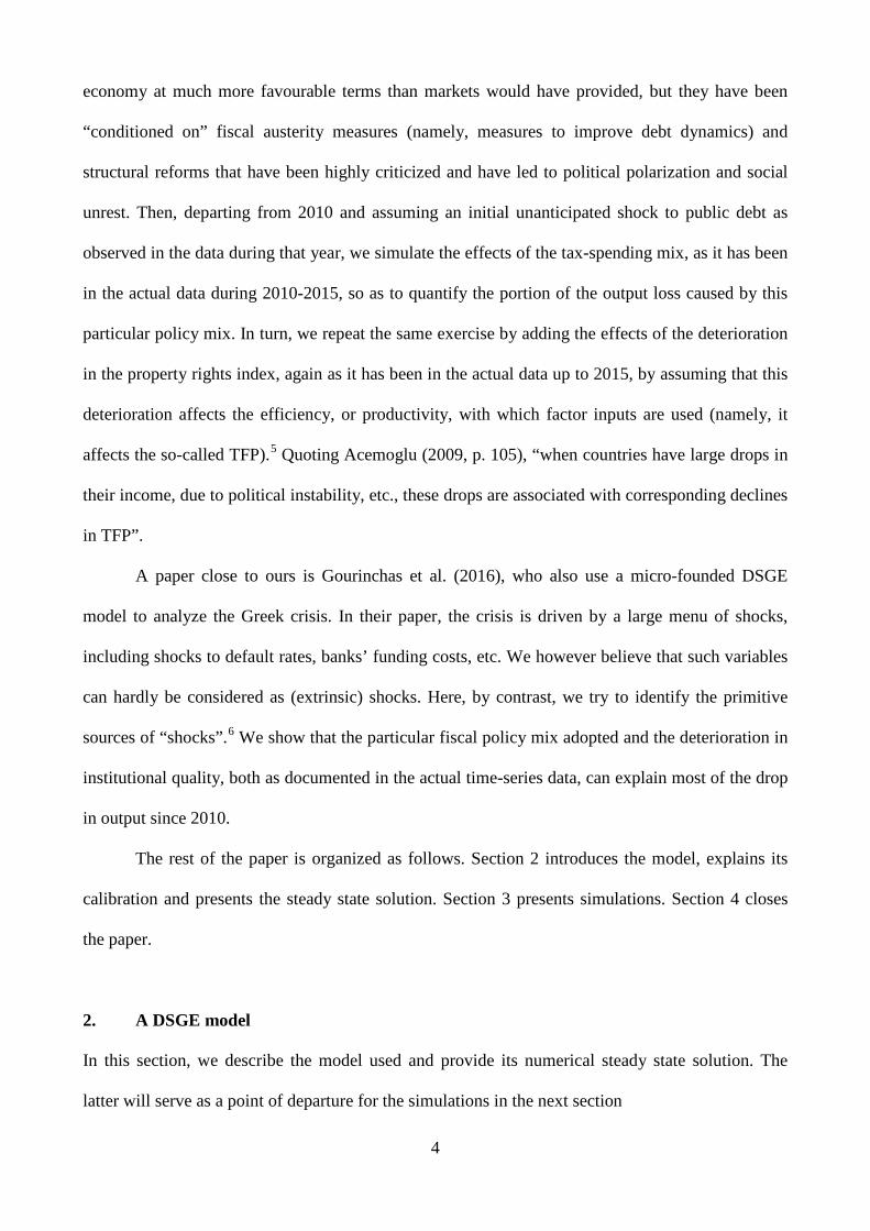
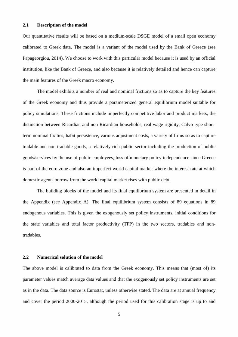
5

21 Description of the model

Our quantitative results will be based on a medium-scale DSGE model of a small open economy

calibrated to Greek data The model is a variant of the model used by the Bank of Greece (see

Papageorgiou 2014) We choose to work with this particular model because it is used by an official

institution like the Bank of Greece and also because it is relatively detailed and hence can capture

the main features of the Greek macro economy

The model exhibits a number of real and nominal frictions so as to capture the key features

of the Greek economy and thus provide a parameterized general equilibrium model suitable for

policy simulations These frictions include imperfectly competitive labor and product markets the

distinction between Ricardian and non-Ricardian households real wage rigidity Calvo-type short-

term nominal fixities habit persistence various adjustment costs a variety of firms so as to capture

tradable and non-tradable goods a relatively rich public sector including the production of public

goodsservices by the use of public employees loss of monetary policy independence since Greece

is part of the euro zone and also an imperfect world capital market where the interest rate at which

domestic agents borrow from the world capital market rises with public debt

The building blocks of the model and its final equilibrium system are presented in detail in

the Appendix (see Appendix A) The final equilibrium system consists of 89 equations in 89

endogenous variables This is given the exogenously set policy instruments initial conditions for

the state variables and total factor productivity (TFP) in the two sectors tradables and non-

tradables

22 Numerical solution of the model

The above model is calibrated to data from the Greek economy This means that (most of) its

parameter values match average data values and that the exogenously set policy instruments are set

as in the data The data source is Eurostat unless otherwise stated The data are at annual frequency

and cover the period 2000-2015 although the period used for this calibration stage is up to and

6

including 2009 (as explained in the Introduction we use pre-crisis euro period data)7 Table A1 in

the Appendix reports the calibrated parameter values and the average values of fiscal policy

variables in the data

Using these numerical values the system is then solved using a Newton-type non-linear

method as implemented in DYNARE (see below for specification of transition dynamics) Its steady

state solution (at least for the key variables) is reported in Table 1 In this solution we have

exogenously set the debt-to-GDP ratio equal to the threshold level 126d equiv which was the value

of the public debt-to-GDP in 2009 (that was the year that risk premia emerged in Greece) so that

one of the remaining fiscal policy instruments needs to be determined residually to satisfy the

within period government budget constraint we assume that it is lump-sum taxes that play this role

As Table 1 shows the solution is in line with data averages over 2000-2009 and can thus provide a

reasonable departure point for the changes that have been taking place since 2010 and are described

in the next sections In particular the solution does a relatively good job at mimicking the position

of the country (and its different sectors) in the international capital market as well as the

consumption-investment behavior of the private sector over the euro pre-crisis years

Table 1 Steady state solution and data averages 2000-09

Variable data solution Total private consumption-to-GDP 065 059

Private investment-to-GDP 018 017 Total work hours 026 026

Work hours in private sector 022 022

Total public debt-to-GDP 126 126 Lump-sum taxestransfers - 0045

Economyrsquos net foreign liabilities-to-GDP 077 066

Private net foreign liabilities-to-GDP 003 0 Exports-to-GDP 023 027

Total imports-to-GDP 034 024

Note (i) Average data over the euro period 2000-2009 with the exception of foreign liabilities which are over the period 2003-2009 and the public debt-to-GDP ratio which is set at its 2009 data value The data source is Eurostat and the Bank of Greece (ii) A positive value of the net foreign liabilities-to-GDP ratio means that the domestic country is a net borrower

7

3 Simulations

As said above departing from the ldquosteady staterdquo solution in Table 2 we will now simulate the

above economy when fiscal policy and institutional quality change as observed in the data after

2010 To understand how the model works we will start by assuming that only fiscal policy has

changed and then we will add changes in institutional quality That is we study one dynamic driver

at a time

31 Effects of the fiscal austerity mix as adopted in practice

In this subsection we will examine other things equal the impact of fiscal consolidation policies as

adopted in Greece since 2010

We work as follows We assume that in 2010 there was an initial shockincrease in the

public debt-to-GDP ratio by 20 pp (as observed in the data) We then set all exogenous fiscal (tax-

spending) instruments as they have actually been in the data during 2010-15 (to isolate the impact

of actual fiscal policy we switch-off the extra feedback reaction to public debt during this sub-

period) Besides in order to mimic the memorandum package we set the interest rate at which the

government borrows from abroad as a weighted average of the risk-free world interest rate and the

world interest rate that the economy would face if it had to borrow from the international capital

market (the latter includes the country risk-premium as in the data)8 The private sector on the other

hand continues to face the full world interest rate (that includes the country risk-premium) when it

borrows from the international market Recall that this premium is a function of the public debt gap

where in this gap the public debt threshold above which premia emerge is 126

We will assume that all the above features continue until the year 2015 (this is the year that

this paper is being written in terms of data availability) Then after 2015 the fiscal instruments are

assumed to gradually return to their pre-crisis 2009 values In particular we assume that they follow

an autoregressive process using as initial values the 2015 values and an autoregressive coefficient

equal to 09 We allow one fiscal instrument to react to the public debt gap (see equation 27) where

8

in this gap the public debt target in the policy rules is the pre-shock value of 126 The interest

rate at which the government borrows from abroad is now allowed to react fully to the degree of

governmentrsquos indebtedness

Thus in our first simulations transition dynamics is driven by the above changes in fiscal

policy We solve the model under perfect foresight (as said above we use a Newton-type non-linear

method as implemented in DYNARE)

The simulated impulse response functions are plotted in Figure 1 while Table 2 summarizes

the associated changes in the main macro variables vis-agrave-vis their values in the data Inspection of

the simulated results in the third column of Table 2 and comparison to the actual data in the second

column implies that the GDP decreases by around 14 between 2009 and 2015 In the data the

actual decrease has been 26 during the same time interval That is the particular fiscal austerity

package which has been adopted between 2010 and 2015 can account for more than half of the big

fall in output observed in the data during this period

Figure 1 Impulse response functions driven by the fiscal austerity package

Note All variables are expressed as percentage deviations from the steady-state with the exception of the CPI inflation the interest rate foreign assets and the public debt-to-GDP ratio that are expressed as percentage point deviations

Year2010 2020 2030 2040

D

evia

tion

-15

-10

-5

0Real Output

Year2010 2020 2030 2040

D

evia

tion

-5

0

5

10Domestic Tradable Output

Year2010 2020 2030 2040

D

evia

tion

-30

-20

-10

0Non-Tradable Output

Year2010 2020 2030 2040

D

evia

tion

-30

-20

-10

0

10Consumption

TotalRicardianNon-Ricardian

Year2010 2020 2030 2040

D

evia

tion

-30

-20

-10

0

10Private Investment

Year2010 2020 2030 2040

D

evia

tion

-6

-4

-2

0Real Wages-Private Sector

2010 2020 2030 2040

P

oint

Dev

iatio

n

-2

-1

0

1CPI Inflation

Year2010 2012 2014 2016 2018

P

oint

Dev

iatio

n

0

1

2

3Interest Rate

Year2010 2020 2030 2040

D

evia

tion

-5

0

5

10Real Exchange Rate

Year2010 2020 2030 2040

D

evia

tion

-20

-10

0

10Trade Volumes

Exports

Imports

Year2010 2020 2030 2040

P

oint

Dev

iatio

n

-6

-4

-2

0

2Foreign Assets

Year2010 2020 2030 2040

P

oint

Dev

iatio

n

-40

-20

0

20

40Public Debt GDP

9

Table 2 Changes in the main macro variables 2015-2009 ()

Variable Data Simulated model with the fiscal package

Simulated model with the fiscal package plus

institutional shocks

Real GDP -26 -137 -22

Real private

consumption

-277 -46 -91

Real private investment -60 -191 -406

Real exchange rate 8 28 -25

Real exports 182 26 -6

Note (i) The changes in the actual time series are computed as log deviations between their 2015 and 2009 values with the exception of real private investment that is computed as 2015 2009 2009( ) I I Iminus The data source is Eurostat Changes in

the simulated series correspond to log deviations from the initial steady state (ii) A positive change for the real effective exchange rate means a real depreciation ie an improvement in the countryrsquos competitiveness

Figure 2 depicts the dynamic paths of fiscal policy instruments under this scenario It thus

confirms the well-recognized feature that the Greek fiscal consolidation program has been based on

both spending cuts and tax rises (see eg European Commission 2015) although the clear rise in all

effective tax rates is particularly striking for a country suffering from a deep recession

Figure 2 Dynamic paths of fiscal policy instruments

Note Government intermediate consumption investment and the public sector wage bill are expressed as shares of the 2009 GDP The effective tax rates are computed following the approach in Papageorgiou et al (2012) The data source is Eurostat

Year2010 2015 2020 2025 2030 2035

007

008

009

01

Government Intermediate Consumption GDP

Year2010 2015 2020 2025 2030 2035

003

004

005

Government Investment GDP

Year2010 2015 2020 2025 2030 2035

01

011

012

013Government Wages GDP

Year2010 2015 2020 2025 2030 2035

017

018

019

02

021Government Transfers GDP

Year2010 2015 2020 2025 2030 2035

016

017

018

019Tax Rate on Consumption

Year2010 2015 2020 2025 2030 2035

036

038

04

Tax Rate on Labour

Year2010 2015 2020 2025 2030 2035

02

022

024

026

Tax Rate on Capital

Year2010 2015 2020 2025 2030 2035

0

002

004

Lump-Sum Taxes

10

Finally we close by reporting that the model would be dynamically unstable (meaning that

there is no solution) if we had assumed that the independently set fiscal policy instruments

remained as they were in the pre-2010 period In other words as said in the Introduction the fiscal

situation was not sustainable and hence some kind of fiscal policy adjustment was unavoidable in

the aftermath of the 2008 world crisis

32 Effects of the deterioration in institutional quality

We will now add another driver of transition dynamics namely changes in institutional quality and

in particular an index that measures the protection of property rights

As said in the Introduction we assume that developments in this index manifest themselves

as shocks to TFP This is a short cut and is similar to the methodology of Chari et al (2007) In

other words as a short cut we construct an ldquoeffectiverdquo TFP series where the degree of

effectiveness is shaped by changes in the degree of property rights protection On the other hand it

should be stressed that it is straightforward to enrich our model so as in the presence of weak

property rights atomistic agents find it to optimal to allocate effort to conflict and extraction and

in equilibrium this leads to resource misallocation that eventually reduces the effective TFP in

Appendix B we provide a simple version of our full-fledged DSGE model that shows this

equivalence formally9 Chari et al (2007) also work with a prototype economy with wedges or

adverse shocks and then show that micro-founded frictions in a more detailed economy manifest

themselves as such wedges or adverse shocks in the prototype economy

We therefore proceed as follows First we construct a series of institutional quality Then

using this we will construct a corresponding series for the effective TFP and finally will feed this

resulting TFP series into our theoretical model in section 2 That is now the modelrsquos dynamics will

be driven both by the fiscal austerity package and the effective TFP series

To construct a measure of the quality of institutions that protect property rights we use the

World Bankrsquos ldquoWorldwide Governance Indicatorsrdquo dataset which has been widely used in many

11

empirical studies (see eg Akitoby and Stratmann (2008) and Baldacci et al (2011)) The

institutional quality index is the sum of the following three indicators ldquorule of lawrdquo ldquoregulatory

qualityrdquo and ldquopolitical stability and absence of violenceterrorismrdquo These indicators are all closely

related to issues concerning the protection of property rights10 Figure 3 shows the evolution of this

composite index over the period 2002-2015 Notice the remarkable decline of institutional quality

after 2008 which was a year of intense social and political turmoil in Greece It should be stressed

that these indicators are not linked (at least directly) to public finances

Figure 3 Deterioration in property rights in Greece (2002-2015)

Note The index is computed as the sum of the following three indicators ldquorule of lawrdquo ldquoregulatory qualityrdquo and ldquopolitical stability and absence of violenceterrorismrdquo The data source is Worldwide Governance Indicators World DataBank

In turn as said above we assume that changes in the TFP level are ldquoshapedrdquo by changes in

the above index of institutional quality In the model there are two specific TFP levels namely in

the tradable and the non-tradable sector We allocate the changes over time in this index to the

respective TFPs according to the relative size of the tradable and non-tradable sectors in the data

(the ratio of the gross value added in the tradable sector to the non-tradable sector is 08) Thus we

obtain time series for the TFP levels in the two sectors and we normalize them so that their values

Year2002 2004 2006 2008 2010 2012 2014

06

08

1

12

14

16

18

2

22

24

12

in 2009 to be consistent with the calibrated values of the TFPs (equal to 1 for the non-tradable and

equal to 09241 for the tradable sector) Figure 4 shows the two constructed effective TFP series

Figure 4 TFP in tradable and non-tradable sectors

ldquoshapedrdquo by the deterioration in property rights

Note The path of the TFP levels is ldquoshapedrdquo by the changes in the institutional quality index according to the relative size of the respective sectors in the data Source Authorsrsquo calculations

Finally using all the above we repeat the same experiment as in section 31 by setting the

TFP levels of tradables and non-tradables over 2010-2015 equal to the constructed series The new

impulse response functions are plotted in Figure 5 while the last column in Table 2 which was

presented above summarizes the associated changes in the main macro variables Notice that now

the reduction in GDP in column 3 of Table 2 is 22 as compared to only 14 without the

TFPinstitutional shock in column 2

Year2009 2010 2011 2012 2013 2014 2015

085

09

095

1

105

TFP Tradable Sector

TFP Non-Tradable Sector

13

Figure 5 Impulse response functions driven by the fiscal austerity package and the deterioration in property rights

Note All variables are expressed as percentage deviations from the steady-state with the exception of the CPI inflation the interest rate foreign assets and the public debt-to-GDP ratio that are expressed as percentage point deviations

4 Conclusions discussion and extensions

In this paper we studied the quantitative importance of the fiscal austerity program and the

deterioration of institutional quality both as observed in the recent data for the Greek great

depression since 2010 The main result is that the adopted fiscal policy mix and the deterioration in

property rights are the main explanatory variables of the Greek great depression

We close with acknowledging two caveats First here we did not explain why the specific

fiscal policy mix has been chosen (which proves to be particularly distorting) or why the society has

chosen to have weak and deteriorating property rights (which leads to misallocation of resources

and hence to a relatively low TFP) In general it is well recognized that the policies chosen andor

the way resources are (mis)allocated are an equilibrium outcome of a political process interacting

with institutions and distribution (see eg Acemoglu (2009 chapter 4) and Jones (2011)) In the

case of Greece there is no shortage of conjectures about the root causes of such choices which go

back to the post-world war II history of the country Second our analysis here was only positive

One could search for instance for alternative fiscal policy mixes andor institutional regimes that

could perhaps mitigate the recessionary effects of debt consolidation We leave these extensions for

future research

Year2010 2020 2030 2040

D

evia

tion

-30

-20

-10

0Real Output

Year2010 2020 2030 2040

D

evia

tion

-15

-10

-5

0

5Domestic Tradable Output

Year2010 2020 2030 2040

D

evia

tion

-40

-30

-20

-10

0Non-Tradable Output

Year2010 2020 2030 2040

D

evia

tion

-60

-40

-20

0Consumption

TotalRicardianNon-Ricardian

Year2010 2020 2030 2040

D

evia

tion

-60

-40

-20

0

20Private Investment

Year2010 2020 2030 2040

D

evia

tion

-30

-20

-10

0Real Wages-Private Sector

2010 2020 2030 2040

P

oint

Dev

iatio

n

-2

0

2

4CPI Inflation

Year2010 2012 2014 2016 2018

P

oint

Dev

iatio

n

0

1

2

3Interest Rate

Year2010 2020 2030 2040

D

evia

tion

-10

-5

0

5Real Exchange Rate

Year2010 2020 2030 2040

D

evia

tion

-20

-10

0

10Trade Volumes

Exports

Imports

Year2010 2020 2030 2040

P

oint

Dev

iatio

n

-4

-2

0

2Foreign Assets

Year2010 2020 2030 2040

P

oint

Dev

iatio

n

-40

-20

0

20

40Public Debt GDP

14

References

Acemoglu D (2009) Modern Economic Growth Princeton University Press Princeton Anderson D Hunt B amp Snudden S (2014) Fiscal consolidation in the euro area How much pain can structural reforms ease Journal of Policy Modeling 36 785-799 Ardagna S (2001) Fiscal policy composition public debt and economic activity Public Choice 109 301-325 Akitoby B amp Stratmann T (2008) Fiscal policy and financial markets Economic Journal 118 1971-1985 Angelopoulos K Philippopoulos A amp Vassilatos V (2009) The social cost of rent seeking in Europe European Journal of Political Economy 25 280-299 Baldacci E Petrova I Belhocine N Dobrescu G amp Mazraani S (2011) Assessing fiscal stress IMF Working Papers WP11100 Washigton DC Bergoeing R Kehoe P Kehoe T and Soto R (2002) Policy driven productivity in Chile and Mexico in the 1980s and 1990s American Economic Review 92 16-21 Blanchard O amp Gali J (2007) Real wage rigidities and the new Keynesian model Journal of Money Credit and Banking 39 35-65 Cacciatore M Duval R amp Fiori G (2012) Short-term gain or pain A DSGE model based analysis of the short-term effects of structural reforms in labour and product markets OECD Economics Department Working Papers no 948 OECD Paris Calvo GA (1983) Staggered prices in a utility-maximizing framework Journal of Monetary Economics 12 383-398 Canova F (2007) Methods for Applied Macroeconomic Research Princeton University Press Princeton CESifo (2016) EEAG Report on the European Economy Munich Chari VV Kehoe P amp McGrattan E (2007) Business cycle accounting Econometrica 75 781-836 Christoffel K Coenen G amp Warne A (2008) The new area-wide model of the Euro area ndash A micro-founded open-economy model for forecasting and policy analysis European Central Bank Working Paper Series Number 944 Christoffel K amp Linzert T (2010) The role of real wage rigidities and labor market frictions for unemployment and inflation dynamics Journal of Money Credit and Banking 42 1435-1446 Christiano LJ amp Eichenbaum M (1992) Current real business cycle theories and aggregate labor market fluctuations American Economic Review 82 430-450 Christiano LJ Eichenbaum M amp Evans C (2005) Nominal rigidities and the dynamic effects of a shock to monetary policy Journal of Political Economy 113 1-45

15

Christiano LJ Trabandt M amp Walentin K (2011) DSGE models for monetary policy analysis In Friedman BM Woodford M (Eds) Handbook of Macroeconomics Volume 3 Elsevier North-Holland 285ndash367 Coenen G Mohr M amp Straub R (2008) Fiscal consolidation in the euro area long run benefits and short-run costs Economic Modeling 25 912-932 Coenen G Straub R amp Trabandt M (2013) Gauging the effects of fiscal stimulus packages in the euro area Journal of Economic Dynamics and Control 32 367-386 Corsetti G Kuester K Meier A amp Muller G (2013) Sovereign risk fiscal policy and macroeconomic stability Economic Journal 123 F99-F132 Duval R (2008) Is there a role for macroeconomic policy in fostering structural reforms Panel evidence for OECD countries over the past two decades European Journal of Political Economy 24 491-502 Economides G Park H amp Philippopoulos A (2007) Optimal protection of property rights in a general equilibrium model of growth Scandinavian Journal of Economics 109 153-175 Economides G Kalyvitis S amp Philippopoulos A (2008) Does foreign aid distort incentives and hurt growth Theory and evidence from 75 aid-recipient countries Public Choice 134 463-488 Economides G Papageorgiou D Philippopoulos A amp Vassilatos V (2013) Smaller public sectors in the Euro Area Aggregate and distributional implications CESifo Economic Studies 59 536-558 Eggertsson G Ferrero A amp Raffo A (2014) Can Structural reforms help Europe Journal of Monetary Economics 61 2-22 Erceg JC amp Linde J (2013) Fiscal consolidation in a currency union Spending cuts vs tax hikes Journal of Economic Dynamics and Control 37 422-445 European Commission (2010) The economic adjustment programme for Greece European Economy Occasional Papers Number 61 Brussels European Commission (2014) Public Finances in EMU Brussels European Commission (2015) Public Finances in EMU Brussels Forni L Monteforte L amp Sessa L (2009) The general equilibrium effects of fiscal policy estimates for the euro area Journal of Public Economics 93 559-585 Forni L Gerali A amp Pisani M (2010a) The macroeconomics of fiscal consolidations in euro area countries Journal of Economic Dynamics and Control 34 1791-1812 Forni L Gerali A amp Pisani M (2010b) Macroeconomic effects of greater competition in the service sector The case of Italy Macroeconomic Dynamics 14 677-708 Forni L amp Pissani M (2013) Macroeconomic effects of sovereign restructuring in a Monetary Union A model-based approach IMF Working Paper Number 13269

16

Gali J Lopez-Salido D amp Valles J (2007) Understanding the effects of government spending on consumption Journal of the European Economic Association 5 227-270 Garcia-Cicco J Pancrazi R amp Uribe M (2010) Real Business Cycles in Emerging Countries American Economic Review 100 2510-2531 Gerali A Notarpietro A and Pisani M (2014) Macroeconomic effects of simultaneous implementation of reforms after the crisis Bank of Italy Working Paper Number 997 Gerali A Notarpietro A amp Pisani M (2015) Structural reforms investment and zero lower bound in a monetary union Manchester School 83 120-139 Gogos S Mylonidis N Papageorgiou D amp Vassilatos V (2014) 1979-2001 A Greek great depression through the lens of neoclassical growth theory Economic Modelling 36 316-331 Gomes S Jacquinot P Mohr M amp Pisani M (2013) Structural reforms and macroeconomic performance in the euro area countries A model-based assessment International Finance 16 23- 44 Gourinchas P-O Philippon T amp Vayanos D (2016) The analytics of the Greek crisis Mimeo London School of Economics Hall R (2003) Wage determination and employment fluctuations NBER Working Paper Number 9967 Hall R (2005) Employment fluctuations with equilibrium wage stickiness American Economic Review 95 50-64 Heylen F Hoebeeck A amp Buyse T (2013) Government efficiency institutions and the effects of fiscal consolidation on public debt European Journal of Political Economy 31 40-59 IMF (2015a) Euro area policies 2015 Article IV consultation Country Report Number 15204 International Monetary Fund Washington IMF (2015b) Fiscal monitor - Now is the time Fiscal policies for sustainable growth International Monetary Fund Washington Jones C (2008) Macroeconomics Norton and Company New York Jones C (2011) Misallocation economic growth and input-output economics NBER Working Paper Number 16742 Kaufmann D Kraay A amp Mastruzzi M (2010) The worldwide government indicators Methodology and analytical issues World Bank Policy Research Working Papers Number 5430 Kehoe T amp Prescott E (2002) Great depressions of the 20th century Review of Economic Dynamics 5 1-18 Kliem M amp Uhlig H (2013) Bayesian estimation of a DSGE model with asset prices Deutsche Bundesbank Discussion Paper Number 372013

17

Malley J Philippopoulos A amp Woitek U (2009) To react or not Fiscal policy volatility and welfare in the EU-3 European Economic Review 53 689ndash714 Mendoza E (2010) Sudden stops financial crises and leverage American Economic Review 100 1941-1966 Mertens K amp Ravn M (2011) Understanding the aggregate effects of anticipated and unanticipated policy shocks Review of Economic Dynamics 14 27ndash54 OECD (2013) Economic Policy Reforms Going for Growth Paris OECD (2015) Economic Policy Reforms Going for growth Paris Papageorgiou D Efthimiadis T amp Konstantakopoulou I (2012) Effective tax rates in Greece Centre of Planning and Economic Research (KEPE) Discussion Paper Series Number 124 Papageorgiou D (2012) Fiscal policy reforms in general equilibrium the case of Greece Journal of Macroeconomics 34 504-522 Papageorgiou D (2014) BoGGEM A dynamic stochastic general equilibrium model for policy simulations Bank of Greece Working Paper Number 182 Papageorgiou D amp Vourvachaki E (2016) Macroeconomic effects of structural reforms and fiscal consolidations Trade-offs and complementarities European Journal of Political Economy Available from httpdxdoiorg101016jejpoleco201608010 Petrongolo B amp Pissarides C (2001) Looking into the black box A survey of the matching function Journal of Economic Literature 38 390-431 Philippopoulos A Vassilatos V and Varthalitis P (2016) Fiscal consolidation in an open economy with sovereign premia and without monetary policy independence International Journal of Central Banking forthcoming Prescott E (2002) Prosperity and depression American Economic Review 92 1-15 Roeger W amp in lsquot Veld J (2013) Expected sovereign defaults and fiscal consolidations European Economy Economic Papers no 479 Schmitt-Groheacute S amp Uribe M (2003) Closing small open economies Journal of International Economics 61 163-185 Schuknecht L von Hagen J amp Wolswijk G (2009) Government risk premiums in the bond market EMU and Canada European Journal of Political Economy 25 371-384 Stahler N amp Thomas C (2012) Fimod ndash A DSGE model for fiscal policy simulations Economic Modelling 29 239-261 Uhlig H (2007) Explaining asset prices with external habits and wage rigidities in a DSGE model American Economic Review 97 239-243 Vogel L (2012) Structural reforms fiscal consolidation and external rebalancing in monetary union A model-based analysis Economic Modelling 29 1286-1298

18

Vogel L (2014a) Nontradable sector reform and external rebalancing in monetary union A model-based analysis Economic Modelling 29 1286-1298 Vogel L (2014b) Structural reforms at the zero bound European Economy Economic Papers no 537

19

1 Namely the drop in output is large occurred rapidly and is sustained this is defined as a ldquogreat depressionrdquo See Gogos et al (2014) for an application of this methodology to the Greek economy before the euro period 2 There is a growing literature on the current Greek crisis For instance Bortz (2015) discusses where the financial assistance has gone offering a different view from that of Sinn (2015) Arellano and Bai (2016) study the Greek default Papageorgiou and Vourvachaki (2016) study the implications of structural reforms in light of the crisis Gourinchas et al (2016) search for shocks that can account for the Greek crisis See below for further details 3 See eg Philippopoulos et al (2016) for the different implications of different fiscal policy mixes used for debt consolidation in Italy 4 Alternatively we could for instance use a VAR approach which requires a limited amount of theory to structure the data (see eg Canova 2007 for methodology) We prefer to follow the DSGE approach so as to have well-defined micro-foundations that allow us to understand the behavioral channels through which exogenous changes affect macroeconomic outcomes 5 There is a large literature that shows how weak institutions affect the efficiency with which factor inputs are used and in particular how weak property rights lead to distortive individual incentives resource misallocation and eventually a lower level of total factor productivity See eg Jones (2008 chapter 4 and 2011) and Acemoglu (2009 chapter 4) for reviews of the literature while see below for further details and references Here working as in Chari et al (2007) we will take a short cut by assuming that changes in property rights directly show up as shocks to TFP nevertheless as argued in subsection 32 below this is equivalent to a richer model where the adverse effect of weak property rights on TFP works via the distortion of individual incentives 6 See eg Chari et al (2007) for a methodology paper on business cycle accounting 7 We focus on the period during which Greece is part of the euro area but before the debt crisis erupted in early 2010 8 In particular we assume that ( ) 1G H

t t tR mR m R= + minus where we set the value of m equal to 05

9 In the same spirit Economides et al (2007 2008) and Angelopoulos et al (2009 2012) also provide micro-founded dynamic general equilibrium models where the presence of weak property rights distorts private incentives and in equilibrium this leads to resource misallocation which in turn maps into reductions in the effective TFP All this belongs to a rich and still growing literature that endogenizes the TFP and hence endogenizes long-term growth 10 The rule of law indicator captures perceptions of the extent to which agents have confidence in and abide by the rules of society and in particular the quality of contract enforcement property rights the police and the courts as well as the likelihood of crime and violence The regulatory quality index captures perceptions of the ability of the government to formulate and implement sound policies and regulations and the credibility of governmentrsquos commitment to such policies The political stability and absence of violenceterrorism indicator captures perceptions of the likelihood that the government will be destabilized or overthrown by unconstitutional or violence means including politically-motivate violence and terrorism For further details see Kaufman et al (2010) We report that each one of these three sub-indexes is highly correlated with key macroeconomic variables such as real GDP and real investment in the Greek data

20

Appendix A A DSGE model and calibration

This appendix presents the model used It is similar to that in Papageorgiou (2014)

1 Households

The economy is populated by a continuum of households of mass one indexed by [ ]01hisin of

which a fraction indexed by [01 ]i λisin minus are referred as ldquoRicardianrdquo or ldquooptimizing householdsrdquo

and a fraction indexed by (1 1]j λisin minus are referred as ldquonon-Ricardianrdquo or ldquoliquidity constrained

householdsrdquo Optimizing households have access to capital and financial markets where they can

invest in the form of physical capital government bonds and internationally traded assets Liquidity

constrained households on the other hand are not able to lend or borrow so that they consume

their disposable labor income in each time period Both households supply differentiated labor

services and act as wage-setters in monopolistically competitive markets

11 Ricardian households

Ricardian households indexed by i have preferences over consumption and leisure The inter-

temporal utility function of each i is

( )10 0

Rt cti i t i t

tU E u C C Hβ ξ

infin

minus

=

= minussum (1)

where (01)β isin is the discount factor i tC is i rsquos effective consumption (defined below) at t i tH is

i rsquos total work hours at t [01)cξ isin is a parameter that measures the degree of external habit

formation in consumption and 1RtC minus denotes average (per household i ) lagged-once effective

consumption Effective consumption is in turn defined to be a linear combination of private

consumption p

i tC and public goods and services (education health etc) provided by the state

sector gtY 1

p g

i t i t tC C Yϑ= + (2)

where [ 11]ϑisin minus is the degree of substitutability between private and public consumption

The instantaneous utility function is assumed to be of the form

( ) ( )1

1 1 log

1

R R i tc ct ti t i t i t

Hu C C H C C

g

ξ ξ κg

+

minus minusminus = minus minus+

(3)

1 See eg Christiano and Eichenbaum (1992) Forni et al (2010a) and Economides et al (2013)

21

where g is the inverse of Frisch labour supply elasticity and 0κ gt is a preference parameter

related to work effort Each household i supplies work hours in the private sector p

i tH and the

public sector gi tH As in eg Ardagna (2001) and Forni et al (2009) hours of work can be moved

across the two sectors and are perfect substitutes in terms of (dis)utility so that p g

i t i t i tH H H= + in

each period t

The Ricardian household can save in the form of physical capital p

i tI domestic government

bonds i tB and foreign assets p

i tF It receives labour income from working in the private sector

p p

i t i tw H and the public sector g gi t i tw H where

pi tw and

gi tw are the real wage rates in the private and

public sector respectively The household rents out capital to firms and receives capital income

k p

t i t i tr u K where ktr is the real return to the effective amount of private capital

pi tK is the physical

private capital stock and 0i tu gt is the utilization rate of capital The household also earns interest

income from domestic government bonds and internationally traded assets that pay a gross nominal

interest 1tR ge and 1HtR ge at 1t + respectively In addition households own all domestic firms so

that they receive their profits as dividends i tDiv Finally each Ricardian household receives a

lump-sum government transfer tri tG The household pays taxes on consumption 0 1c

ttlt lt on

labour income 0 1lttlt lt on capital earnings and dividends 0 1k

ttlt lt and lump-sum taxes tT

Hence the budget constraint of each Ricardian household i is

( )

( )( ) ( )( )

1 1

1

1

1 1

pIi t t i tc p pt

t i t i tC C Ct t t

l p p g g k k pt i t i t i t i t t t i t i t i t

t

B S FPC IP P P

w H w H r u K Div

R

t

t t

+ +

minus

+ + + + =

= minus + + minus + +

+ 1

pi t t i tH tr h

t i t t i tC Ct t

B S FR G T

P Pminus+ + minus minusG

(4)

where CtP and I

tP are the prices of a unit of the private consumption final good and the investment

final good respectively and tS is the nominal exchange rate (expressed in terms of domestic

currency per unit of foreign currency) The household faces costs when it adjusts its private foreign

asset holdings hi tG whenever the private foreign assets-to-GDP ratio GDP

tY

t

ptit

YPFS 1 + deviates from its

long-run target level f In particular

( )2

1 1

2

pY GDPft i th p Y GDP C t t

i t t i t t t t C Y GDPt t t

S FP YS F P Y P fP P Y

ξ ++

G = minus

(5)

22

where GDPtY is the economyrsquos real GDP Y

tP is the GDP deflator and 0gefξ is an adjustment cost

parameter2

The private capital stock evolves over time according to the following law of motion

( )( ) 1

1

1 1p

i tp p p I pi t i t i t i tp

i t

IK u K I

Iδ+

minus

= minus + minusΨ

(6)

where IΨ is a convex adjustment cost function for investment as in eg Christiano et al (2005)

2

1 1

12

p pki t i tIp p

i t i t

I II I

ξ

minus minus

Ψ = minus

(7)

where (1) (1) 0I IΨ = Ψ = and 0kξ ge is an adjustment cost parameter We assume that the

depreciation rate of private capital depends on the rate of capacity utilization and is a convex

function that satisfies 0pδ prime gt 0pδ primeprime gt so that ( ) p p

i t i tu uϕδ δ= where (01)pδ isin and 0ϕ gt are

respectively the average rate of depreciation of private capital and the elasticity of marginal

depreciation cost

The first-order conditions of this problem are written below when we present the final

equilibrium system

12 Non-Ricardian households

Liquidity constrained households indexed by j have the same preferences as Ricardian

households They receive labour income from working in the private and public sectors but have no

access to capital or financial markets so that in each period their consumption spending equals

their after-tax wage income plus lump-sum government transfers The period-by-period budget

constraint of each household j is

( ) ( )( ) 1 1c l p p g g trt j t t j t j t j t j t j tC w H w H Gt t+ = minus + + (8)

where pj tH and

gj tH are respectively hours worked in the private and public sector by household j

and trj tG is a lump-sum government transfer to each j Thus as in eg Coenen et al (2013) we

allow for a potentially uneven distribution of government transfers across Ricardian and non-

Ricardian households

The first-order conditions of this problem are written below when we present the final

equilibrium system

2 This specification ensures that foreign private assets are stationary see eg Schmitt-Grohe and Uribe (2003)

23

2 Wage setting and the evolution of wages in the private sector

We assume that wages in the private sector are set by monopolistic unions as in eg Forni et al

(2009) and Gali et al (2007) More specifically households supply differentiated labour varieties to

a continuum of unions [ ]01hisin each of which represents a specific labour variety Every variety is

uniformly distributed across households so that each union ultimately represents 1 λminus fraction of

Ricardian households and λ of non-Ricardian households In every period each union sets the

wage rate for its own workers by trading off the utility derived from private sector labour income

and the disutility of total work effort by taking into account the demand for the differentiated labour

variety h At the same time private and public sector firms allocate their labour demand uniformly

across the h labour varieties independently of the type of households which implies that hours

worked by each type of household are equal

h p h p pj t i t h tH H H= equiv and

h g h g gj t i t h tH H H= equiv 3

Therefore in each period a typical union h chooses the wage rate ph tw to maximize

( ) ( ) ( )1

1 1 1

1h tNR l p p R l p p

w h t h t h t h t h t h t

HL w H w H

g

λ t λ t κg

+

= L minus + minus L minus minus + (9a)

subject to

1

Wt

Wt

ph tp p

h t tpt

wH H

w

micromicro

minusminus

=

(9b)

p g

h t h t h tH H H= + (9c)

where Eq (9b) is the demand for the differentiated labour input h ptH is total labour demand in the

private sector ptw is the aggregate wage rate in the private sector and

NRh tL

Rh tL are the marginal

utilities of consumption of non-Ricardian and Ricardian households of labour variety h

respectively used as weights Finally ( ) 1 1W Wt tmicro micro minus gt is the elasticity of substitution across the

differentiated labour services where 1Wtmicro gt is the wage markup in the private labour market

Focusing on a symmetric equilibrium in which all unions choose the same wage rate ex

post the first-order condition of the above problem is

1p Wt tNR R

t t

wMRS MRS

λ λ micro minus

+ =

(10)

3 Total public sector labour demand for the differentiated labour input ℎ is exogenous and is defined as 1

0

g gt h tH H dh= int

24

where ptw is the optimal wage rate chosen by unions and NR

tMRS and RtMRS are the marginal

rates of substitution between consumption and leisure of non-Ricardian and Ricardian households

respectively4

Following eg Hall (2005) and Blanchard and Gali (2007) we introduce further rigidities in

the labour market by assuming that real wages respond sluggishly to labour market conditions In

particular the real wage rate in the private sector is modeled as a weighted average of the lagged-

once real wage rate and the optimal real wage rate chosen by unions

( ) ( )11

n np p pt t tw w w

minus

minus= (11)

where 0 1nle le denotes the degree of real wage rigidities and ptw is given by (10)5 This

formulation aims to capture the rigidities found in the Greek labour market (see eg the discussion

in European Commission 2010)6

3 Production in the private sector

There are two types of domestic firms The first type consists of monopolistically competitive firms

that produce intermediate goods tradable and non-tradable The continuum of firms producing

differentiated varieties of tradables indexed by [ ]01Tf isin sell their output domestically or abroad

(the latter are recorded as exports) The continuum of firms producing differentiated varieties of

non-tradables indexed by [ ]01Nf isin sell their output domestically only There is also a continuum

of monopolistically competitive firms importing intermediate goods indexed by [ ]01Mf isin The

second type of firms consists of four perfectly competitive firms that produce final goods These

firms combine purchases of intermediate goods to produce four non-tradable goods a private

consumption good a private investment good a public consumption good and a public investment

good Finally there is a foreign final goods firm that combines purchases of the exported domestic

intermediate goods

4 Note that when 0λ = ie when all households are Ricardian W

tmicro reduces to a markup of the optimally chosen real

wage rate over the marginal rate of substitution between consumption and leisure of Ricardian households 5 See also eg Uhlig (2007) Malley et al (2009) and Kliem and Uhlig (2013) for a similar specification Microfoundations for Eq (11) can be found in eg Hall (2003) Petrongolo and Pissarides (2001) and Christoffel and Linzert (2010) 6 Papageorgiou (2014) finds that this specification can capture rather well the aggregate dynamics of work hours and real wages in Greece

25

31 Final goods firms

As said above there are four representative final goods firms that combine purchases of tradable

intermediate goods with non-tradable goods to produce a private consumption good ptC a private

investment good ItI a public consumption good gc

tG and a public investment good gitG

Private consumption goods producer

The representative producer of the private final consumption good combines a bundle of tradable

consumption intermediate goods TtC with a bundle of non-tradable intermediate goods N

tC

according to a constant elasticity of substitution (CES) production function

( ) ( )1 11 1 1

(1 )

C

C C CC CC C

p T Nt C t C tC C C

εε ε ε

ε εε εω ωminus minus minus

= + minus

(12)

where [ ]01Cω isin measures the weight of tradable goods in the production of the final private

consumption good and 0Cε gt is the elasticity of substitution between tradable and non-tradable

consumption goods

In turn the tradable intermediate consumption good bundle is a CES function of the

domestically produced bundle of tradable intermediate consumption goods DtC and the bundle of

imported intermediate consumption goods MtC

( ) ( )1 11 1 1

(1 )

TC

TC TC TCTC TCTC TC

T D Mt TC t TC tC C C

εε ε ε

ε εε εω ωminus minus minus

= + minus

(13)

where [ ]10isinTCω measures the home bias in the production of the tradable intermediate

consumption good and 0TCε gt is the elasticity of substitution between domestic and imported

intermediate consumption goods

The intermediate consumption good bundles that are used as inputs combine differentiated

varieties supplied by intermediate good firms Specifically the varieties supplied by each tradable

intermediate goods firm Tf T

Df t

C each non-tradable intermediate-goods firm Nf N

Nf t

C and each

importing firm Mf M

Mf t

C are respectively combined using a CES technology into

( )1

1

0

Tt

Tt

TD D Tt f t

C C dfmicro

micro

= int (14a)

26

( )1

1

0

Nt

Nt

NN N Nt f t

C C dfmicro

micro

= int (14b)

( )1

1

0

Mt

Mt

MM M Mt f t

C C dfmicro

micro

= int (14c)

where 1T N Mt t tmicro micro micro gt are the intra-temporal elasticities of substitution between different varieties

within each type of intermediate consumption good As we show below T N Mt t tmicro micro micro represent

markups in the markets of domestic and imported intermediate goods

Given the above technology the producer of the final private consumption good solves a

three stage problem In the first stage it takes as given the prices of domestic tradable N

Df t

P non-

tradable T

Nf t

P and imported intermediate goods M

Mf t

P and chooses the amounts of the

differentiated goods T

Df t

C N

Nf t

C M

Mf t

C in order to minimize total expenditures for the bundles of

the differentiated goods 1

0

T TD D Tf t f t

P C dfint 1

0

N NN N Nf t f t

P C dfint 1

0

M MM M Mf t f t

P C dfint subject to the aggregation

constraints in (14a)-(14c) The solution of the cost minimization problem gives the demand

functions for these intermediate goods Tf Nf and Mf respectively

1

Dt

DtT

T

Df tD D

tDf tt

PC C

P

micromicro

minusminus

=

(15a)

1

Nt

NtN

N

Nf tN N

tNf tt

PC C

P

micromicro

minusminus

=

(15b)

1

Mt

MtM

T

Mf tM M

tMf tt

PC C

P

micromicro

minusminus

=

(15c)

where D N Mt t tP P P are the aggregate price indices of domestic tradable non-tradable and imported

intermediate consumption goods respectively

In the second stage the firm chooses the bundles DtC and M

tC in order to maximize its

profits 1C TC T D D M Mt t t t t t tP C P C P CP = minus minus subject to the technology constraint (13) and by taking as

given the price indexes of domestic tradables TCtP non-tradables D

tP and imported intermediate

consumption goods MtP Thus it solves

27

max

D Mt t

TC T D D M Mt t t t t t

C CP C P C P Cminus minus

subject to

( ) ( )1 11 1 1

(1 )

TC

TC TC TCTC TCTC TC

T D Mt TC t TC tC C C

εε ε ε

ε εε εω ωminus minus minus

= + minus

In the third stage the firm chooses the demand for TtC and N

tC to maximize profits

2C C C TC T N Nt t t t t t tP C P C P CP = minus minus subject to the technology constraint (12) and by taking the input

prices CtP TC

tP and NtP as given Thus it solves

max

T Nt t

C C TC T N Nt t t t t t

C CP C P C P Cminus minus

subject to

( ) ( )1 11 1 1

(1 )

C

C C CC CC C

p T Nt C t C tC C C

εε ε ε

ε εε εω ωminus minus minus

= + minus

The demand functions for domestic tradable and imported consumption goods as well as for

tradable and non-tradable intermediate consumption goods resulting from the optimization problem

of the final consumption good firm are

TCD Dt t

TCT TCt t

C PC P

ε

ωminus

=

(16a)

( )1TCM M

t tTCT TC

t t

C PC P

ε

ωminus

= minus

(16b)

CT TCt t

CC Ct t

C PC P

ε

ωminus

=

(16c)

( )1CN N

t tCC C

t t

C PC P

ε

ωminus

= minus

(16d)

From the zero profit condition we get the price index for tradable consumption goods

( ) ( )( )1

1 1 11TC TC TCTC D M

t TC t TC tP P Pε ε εω ω

minus minus minus = + minus and the price index of a unit of the final consumption

good (ie the Consumption Price Index) ( ) ( ) ( )1

1 1 11C C CC TC N

t C t C tP P Pε ε εω ω

minus minus minus = + minus where

D N Mt t tP P P are the prices of domestic tradable intermediates non-tradable intermediates and

imported intermediate goods respectively

28

Private investment goods producer

Optimal decisions regarding the production of the final private investment good are derived in an

analogous manner as above The representative producer of the private investment good combines a

composite bundle of tradable intermediate goods TtI with a bundle of non-tradable intermediate

goods NtI to generate a composite final private investment good I

tI by using a constant elasticity

of substitution (CES) production function

( ) ( )1 11 1 1

(1 )

I

I I II II I

I T Nt I t I tI I I

εε ε ε

ε εε εω ωminus minus minus

= + minus

where [ ]01Iω isin measures the weight of tradable goods in the production of the final private

investment good and 0Iε gt is the elasticity of substitution between tradable and non-tradable

investment goods

In turn the composite bundle of the tradable intermediate investment good that is used in the

production of final investment goods is a CES function of domestically produced tradable

intermediate investment goods DtI and imported intermediate investment goods M

tI

( ) ( )1 1 11 1

(1 )

TI

TITI TITI TITI TI

T D Mt TI t TI tI I I

εεε ε

ε εε εω ωminusminus minus

= + minus

where [ ]01TIω isin measures the home bias in the production of the tradable intermediate

consumption good and 0TIε gt is the elasticity of substitution between domestic and imported

investment goods

The demand functions for domestic tradable and imported investment goods as well as for

tradable and non-tradable investment goods are

TID Dt t

TIT TIt t

I PI P

ε

ωminus

=

( )1TIM M

t tTIT TI

t t

I PI P

ε

ωminus

= minus

IT TIt t

II It t

I PI P

ε

ωminus

=

( )1IN N

t tIT I

t t

I PI P

ε

ωminus

= minus

29

where ( ) ( )( )1

1 1 11TI TI TITI D M

t TI t TI tP P Pε ε εω ω

minus minus minus = + minus and ( ) ( )( )

11 1 11

I I II TI Nt I t I tP P P

ε ε εω ωminus minus minus = + minus

are respectively the price indices for tradable intermediate investment goods and final investment

goods

Public consumption and investment goods production

Regarding the final public consumption and investment goods gctG and gi

tG we assume they are

produced using only non-tradable intermediate goods Hence gc Nt tG GC= and gi N

t tG GI= where

( )1

1

0

Nt

Nt

NN N Nt f t

GC GC dfmicro

micro

= int and ( )

11

0

Nt

Nt

NN N Nt f t

GI GI dfmicro

micro

= int

The optimal demand functions are

1

Nt

NtN

N

Nf tN N

tNf tt

PGC GC

P

micromicro

minusminus

=

and 1

Nt

NtN

N

Nf tN N

tNf tt

PGI GI

P

micromicro

minusminus

=

Aggregating across final good producing firms we get the respective aggregate domestic demand

functions for non-tradable domestic tradable and imported intermediate goods Tf Nf and mf

1

Nt

NtN

N N N N N

Nf tNT N N N N NT

tNf t f t f t f t f tt

PY C I GC GI Y

P

micromicro

minusminus

= + + + =

1

Tt

TtT

T T T

Df tD D D D

tDf t f t f tt

PY C I Y

P

micromicro

minusminus

= + =

1

Mt

MtM

M M M

mf tM M M M

tmf t f t f tt

PY C I Y

P

micromicro

minusminus

= + =

where NT N N N Nt t t t tY C I GC GI= + + + D D D

t t tY C I= + and M M Mt t tY C I= + are respectively the total

demand for non-tradable goods total domestic demand for domestically produced tradable goods

and total demand for imports

32 Intermediate goods firms

Each tradable and non-tradable intermediate good Tf t

Y and Nf t

Y is produced by a continuum of

monopolistically competitive intermediate goods firms indexed by [ ]01Tf isin and [ ]01Nf isin

respectively according to the production technologies

30

( ) ( ) ( )1

T T G

T T T

a a aT gt t Tf t f t f t

Y A K H Kminus

= minusΦ (17a)

( ) ( ) ( )1

N N G

N N N

a a aN gt t Nf t f t f t

Y A K H Kminus

= minusΦ (17b)

where Tf t

K is private capital Tf t

H is work hours in the private sector gtK is public capital

0T Na a gt are the output elasticities of capital services in the tradable and non-tradable sectors

respectively and 0Ga gt is the output elasticity of public capital7 Finally 0T NΦ Φ ge are fixed

costs of production and TtA N

tA are sector-specific total factor productivity levels

Tradable sector

In what follows we present the problem of intermediate goods firms in the tradable sector

Domestic intermediate goods firms in the tradable sector solve a two-stage problem In the first

stage each firm takes as given factor prices ktr and p

tw and chooses capital and labour inputs

Tf tK and

Tf tH in order to minimize total real input cost We also introduce a working capital

channel in the form of a ldquocash-in-advancerdquo constraint in the spirit of eg Mendoza (2010) In

particular at the beginning of each period each firm borrows from international lenders in order to

cover a fraction (01)tv isin of their total labour costs in advance of revenuesrsquo receipt The working

capital loan is repaid by the end of the period at the domestic country gross interest rate HtR Thus

the intratemporal problem of each firm involves the minimization of their costs inclusive of the

costs of serving their intra-period working capital loan In other words

( )

min 1T T TT Tf t f t

k p H pt t t t tf t f t f tK H

r K w H R v w H+ + minus (18)

subject to (17a)

The first-order conditions are

( )( ) ( )

1 1 1T

T

T

Tf tH pt t t T f t

f t

YR w a mc

Hν

+Φ+ minus = minus (19)

T

T

T

Tf tkt T f t

f t

Yr a mc

H

+Φ= (20)

where Tf t

mc is the Lagrange multiplier associated with the technology constraint that is the real

marginal cost in terms of the consumer prices CtP Because firms borrow to cover part of their

7 These production functions have increasing returns to scale with respect to all inputs and constant returns to scale with respect to private inputs (see also eg Baxter and King (1993) and Leeper et al (2010))

31

labour costs the marginal cost of labour is higher than the wage rate in the private sector As a

result increases in either the share of labour costs that are financed through working capital loans

or in the domestic interest rate directly increase the cost of labour and thereby reduce labour

demand

The labour input Tf t

H is a composite aggregate of household-specific varieties T

hf t

H

( )1

1

0

Wt

Wt

T Th

f t f tH H

micro

micro

= int Optimal demand is

1

Wt

T T

ph thpf t f t

t

wH H

w

micro =

where ( 1) 1W Wt tmicro micro minus gt is the

elasticity of substitution across differentiated labour services and ptw is the aggregate real wage

index in the private sector that is given by ( )11

1 10

Wt

Wtp p

t h tw wmicro

micro

minus

minus

= int

In the second stage intermediate good firms in the tradable sector choose the price that

maximizes discounted real profits As in Christoffel et al (2008) firms charge different prices at

home and abroad setting prices in producer currency In both domestic and foreign markets we

assume that prices are sticky aacute la Calvo (1983) In particular each period t the firm Tf optimally

resets prices with a constant probability 1 Dpθminus when it sells its differentiated product in the

domestic market and with probability 1 Xpθminus when it sells its product abroad The firms that cannot

optimize partially index their prices to aggregate past inflation according to the price indexation

schemes ( )1 1

D

T T

xD D Dtf t f t

P P minusminus= P and ( )1 1

X

T T

xX X Xtf t f t

P P minusminus= P where

TDf t

P denote the domestic price of

good Tf T

Xf t

P its foreign price and 1D D Dt t tP PminusP = 1X X X

t t tP PminusP = where D Xt tP P are the

aggregate domestic and export price indices (defined below) respectively The indexation

parameters [ ] 01D Xx x isin determine the weights given to past inflation

Each firm Tf which can optimally reset its price in period t knows with probability Dpθ

that this price will continue to be in effect t periods ahead and so chooses the optimal price

TD

f tP

to maximize the discounted sum of expected real profits (in terms of consumer prices CtP ) by

taking aggregate domestic demand DtY and the aggregate price index in the domestic market D

tP

as given Thus each firm Tf maximizes

( ) ( )

1

0 1

maxTD

TDTf t

DR Dx f tD D D Dt tt p t s tR D Df tP st t t

P PE mc YP P

t tt t

t tt t t

βθinfin

+ ++ minus + +

= = + +

L P minus L sum prod (21)

32

subject to

( )1

1

1

Tt

TtTD

T

Dx f tD D D

t s tDf ts t

PY Y

P

t

t

micromicrot

tt

+

+

minusminus

+ minus += +

= P prod (22)

where D C T Dt t t tmc P mc P= is the real marginal cost in terms of the domestic price index and

R Rt tt+L L is the ratio of the marginal utilities of consumption of Ricardian households - that are the

owners of the firms - according to which firms value future profits8 Notice that since all firms face

the same marginal cost and take aggregate variables as given any firm that optimizes will set the

same price

TD D

tf tP P=

Thus the first-order condition of the above problem is

( ) ( ) ( )1

1 1

1 1

0

Tt

TD Dtx xD DR D D D

t s t sD D T Dt t t tt p t t tR D D D D D

s st t s t t t s t

P P PE Y mcP P P

t

t

micromicro

t tt t tt t t

t

βθ micro

+

+

minusminus

+ minus + minus+ ++ + +

= =+ + +

P PL minus = L P P

prod prod (23)

According to the above expression firms set nominal prices so as to equate the average future

expected marginal revenues to average future expected marginal costs9 The aggregate domestic

index evolves according to ( )( ) ( )( )111

1 11 11

Tt

TDT ttxD D D D D D

t p t p t tP P Pmicro

micromicroθ θ

minus

minusminusminus minus

= minus + P

Similarly the associated first-order condition of each firm Tf that chooses its price in the

foreign market in period t is

( ) ( ) ( )1

1 1

1 1

0

Xt

XX Xtx xX XR X X X

t s t sX X X Xt t t tt p t t tR X X C X X

s st t s t t t s t

P P PE Y mcP P P

t

t

micromicro

t tt t tt t t

t

βθ micro

+

+

minusminus

+ minus + minus+ ++ + +

= =+ + +

P PL minus = L P P

prod prod (24)

where X C T Xt t t tmc P mc P= is the real marginal cost in terms of the aggregate export price index and

the aggregate export price index is ( )( ) ( )( )111

1 11 11

Xt

XXx ttxX X X X X X

t p t p t tP P Pmicro

micromicroθ θ

minus

minusminusminus minus

= minus + P

8 In equilibrium the marginal utility of consumption is common across Ricardian households

Ri t tL = L

9 In the case of fully flexible prices 0Dpθ = the above condition reduces to the static relation D T C T

t t t tP P mct tmicro + +=

which states that the price is equal to a markup over the nominal marginal cost

33

Non-tradable sector

The optimal demand by each firm Nf for labour of type h is

1

Wt

Wt

N N

ph thpf t f t

t

wH H

w

micromicro

minusminus

=

and the

aggregate demand for labour of type h is

11

0

Wt

Wt

N

ph tN h N

h t tpf tt

wH H df H

w

micromicro

minusminus

= =

int where NtH is total

labour demand in the non-tradable intermediate good sector As in the case of the tradable good

firms non-tradable intermediate good firms take short-term loans from international lenders at the

home countryrsquos gross interest rate HtR in order to finance a fraction tv of their total labour costs

To minimize costs each firm takes as given the factor prices ktr and p

tw and chooses N Nf t f t

K H

in order to minimize total real input cost ( ) 1N N N

k p H pt t t t tf t f t f t

r K w H R v w H+ + minus subject to the

production function The first-order conditions are

( )( ) ( )

1 1 1N

N

N

Nf tH pt t t N f t

f t

Yv R w a mc

H

+Φ+ minus = minus

N

N

N

Tf tkt N f t

f t

Yr a mc

K+Φ

=

where due to symmetry N

Ntf t

mc mc=

Non-tradable intermediate good firms face price stickiness aacute la Calvo with 1 Npθminus being the

probability that a firm Nf can optimally reset its price in any given period 0t ge The optimal

pricing is characterized by the following conditions

( ) ( ) ( )1

1 1

1 1

0

Nt

Nd Ntx xN NR N N N

t s t sN N N Nt t t tt p t t tR N N C N N

s st t s t t t s t

P P PE Y mcP P P

t

t

micromicro

t tt t tt t t

t

βθ micro

+

+

minusminus

+ minus + minus+ ++ + +

= =+ + +

P PL minus = L P P

prod prod

and the aggregate domestic index evolves according to

( )( ) ( )( )111

1 11 11

Nt

NNN ttxN N N N N N

t p t p t tP P Pmicro

micromicroθ θ

minus

minusminusminus minus

= minus + P

Importing firms

There is a continuum of importing firms [ ]01Mf isin each of which imports a single differentiated

intermediate good M

Mf t

Y These firms operate under monopolistic competition so that they have

34

pricing power This creates a wedge between the price at which the importing firms buy the foreign

differentiated goods in the world markets Yt tS P and the price at which they sell these goods to

domestic households M

Mf t

P Importing firms face price stickiness aacute la Calvo with 1 Mpθminus being the

probability that a firm Mf can optimally reset its price in the domestic market in any given period

0t ge so that optimal pricing follows

( ) ( ) ( )1

1 1

1 1

0

Mt

Mm mtx xM MR M M M

t s t sm M M Mt t t tt p t t tR M M C M M

s st t s t t t s t

P P PE Y mcP P P

t

t

micromicro

t tt t tt t t

t

βθ micro

+

+

minusminus

+ minus + minus+ ++ + +

= =+ + +

P PL minus = L P P

prod prod

and the aggregate import price index evolves according to

( )( ) ( )( )111

1 11 11

Mt

MmM ttxM m M m M M

t p t p t tP P Pmicro

micromicroθ θ

minus

minusminusminus minus

= minus + P

33 Demand from foreign final goods firms

We now model the demand coming from foreign firms or equivalently specify the domestic

countryrsquos exports Recall that the domestic economy produces intermediate tradable goods that are

also exported and so we need to model a final goods firm that transforms them into final goods

There is a representative foreign final good firm that purchases the differentiated exported goods

X

f tY produced by the domestic tradable intermediate good firms Tf and transforms them into a

homogeneous final good XtY via the CES technology

( )1

11

0

XtX

tT

X X Tt f t

Y Y dfmicro

micro

= int (25)

where 1Xtmicro gt is related to the intratemporal elasticity of substitution between the differentiated

outputs supplied by domestic intermediate good firms ( ) 1 1X Xt tmicro micro minus gt

The foreign firm takes the prices of exported differentiated goods

TX

tf tP S (expressed in

terms of the foreign currency) as given and chooses the optimal amounts of differentiated inputs to

minimize total input costs ( )1

0T T

X X Ttf t f t

P S Y dfint subject to (25) so that the optimal demand function

for each input T

Xf t

Y is 1

Xt

XtT

T

Xf tX X

tXf tt

PY Y

P

micromicro

minusminus

=

where ( )11

11

0

Xt

Xt

TX X T

t f tP P df

micro

micro

minus

minus

= int is the aggregate

price index of exported domestic intermediate goods and XtY is total foreign demand for domestic

35

intermediate goods The latter is

XX

X t tt tX

t

P SY YP

εminus

=

where X

tP is the price of foreign

competitors in the export markets tY is foreign economy output and 0Xε gt is the price elasticity

of export demand

4 The public sector

We now model the public sector

41 Government budget constraint and fiscal policy instruments

The government levies taxes on consumption labour income capital earnings and dividends We

also assume lump-sum taxestransfers The government also sells one-period government bonds to

the domestic bond market 1gtB + and the international market 1

gtF + Total tax revenues plus the issue

of new government bonds are used to finance government consumption ctG investment i

tG

transfers trtG and the wage bill of public sector employees g g

t tw H Moreover the interest rates

that the government pays on inherited domestic public debt and on foreign public debt are tR and

GtR respectively We assume that G

tR is a weighted average of the market interest rate that the

country faces when it borrows from abroad and the risk-free world interest rate (see below for

details) Thus the within-period government budget constraint in per-capita terms is

( ) ( )1 1

1 1

g gc p l p p g g k k pt t tt t t t t t t t t t t t tc C

t tN N g g

c i tr g g Gt t t t tt t t t t t tC C C C

t t t t

B S F C w H w H r u K Div TP P

P P B S FG G G w H R RP P P P

t t t+ +

minus minus

+ + + + + + + =

= + + + + +

(26)

Therefore the government has eleven policy instruments 1 1 c l k g g c i tr g gt t t t t t t t t t t tX T w H G G G B Ft t t + +isin

out of which ten can be exogenously set

To ensure dynamic stability we need to assume that one of the exogenously set fiscal policy

instruments follows a state-contingent rule reacting systematically to deviations of the public debt-

to-GDP ratio from a target level and the rate of change of debt

( ) ( )1 1 2 1d y d y y

t t t t tX X D d D Dφ φminus minus= + minus + minus (27)

where 1 1

y tt y GDP

t t

DDP Yminus minus

equiv denotes the debt-to-GDP ratio in the beginning of period t d is a target value

of the public debt-to-GDP ratio (see below for details) and 1 2 0d dφ φ gt are feedback policy reaction

coefficients (as in a Taylor rule for the nominal interest rate)

36

For notational convenience we will define the share of total public debt held by domestic

agents at the end of period t as 1

1

gt

tt

BD

ζ +

+

equiv where 0 1tζle le so that 1 1(1 )gt t t tS F Dζ+ += minus and

1 1 1g g

t t t tD B S F+ + += +

42 Production of public goodsservices

On the production side following eg Forni et al (2010a) and Economides et al (2013 2016) we

assume that the government combines public spending on goods and services ctG and public

employment gtH to produce public goodsservices g

tY according to the production function

( ) ( )1g c gt t t tY A G H

c cminus= (28)

where 0 1cle le is a technology parameter

The law of motion of public capital in per-capita terms is

( )1 1g g g it t tK K Gδ+ = minus + (29)

where ( )01gδ isin is the depreciation rate of public capital stock and 0 0gK gt is given

Regarding the inputs used in the above production function ctG is produced by final good

firms that use only non-tradable intermediate goods as inputs (see above) while gtH is total public

sector demand for the differentiated labour variety h that is exogenous (see above)

5 World capital markets and sovereign spreads

Following most of the literature on small open economies we assume that when domestic

households and the government participate in the world capital market they face an interest rate

that is public debt elastic (see eg Schmitt-Grohe and Uribe 2003)

In particular the nominal interest rate at which the country borrows from the international

market HtR bears a risk-premium term 0tψ ge that introduces a wedge between the interest rate

that the home country faces and the risk-free world nominal interest rate tR

max Ht t t tR R Rψ= + (30)

where as in eg Christiano et al (2011) Garcia-Cicco et al (2010) and Philippopoulos et al

(2016) the risk-premium is assumed to be an increasing function of public debt imbalances

( )( )1exp 1d yt tD dψ ψ += minus minus (31)

where 0dψ ge is a risk parameter and 0d gt is an exogenous threshold above which premia

emerge Thus when the public debt-to-GDP ratio is above a threshold level an interest rate spread

37

arises which is consistent with empirical evidence (see eg Ardagna et al 2008 Roeger and inrsquot

Veld 2013 Schuknecht et al 2009 Corsetti et al 2013) Conceptually the risk premium

component on the right hand side of (31) reflects the risk of sovereign or country default and thus

provides a channel through which such a risk affects directly the real economy

6 Monetary-exchange rate policy regime

We model the domestic economy as a member of a currency union in the sense that the nominal

exchange rate tS is exogenously set and at the same time there is no monetary policy

independence The latter means that the domestic nominal interest rate on government bonds tR is

determined endogenously (see eg Philippopoulos et al (2016) for details)

7 Aggregation and market-clearing conditions

71 Aggregation

The aggregate quantity expressed in per-capita terms of any household specific variable h tX is

given by ( )1

01t h t i t j tX X dh X Xλ λ= = minus +int Thus per capita private consumption is given by

( ) 1p p pt i t j tC C Cλ λ= minus + Since only optimizing households have access to the capital bond

dividend and international markets the per capita quantities for private capital private investment

domestic government bonds foreign private assets and profits are respectively ( ) 1p pt i tK Kλ= minus

( ) 1t i tI Iλ= minus ( ) 1t i tB Bλ= minus ( ) 1p pt i tF Fλ= minus and ( ) 1t i tDiv Divλ= minus Per capita government

transfers are ( ) 1tr tr trt i t j tG G Gλ λ= minus + where total transfers are allocated between optimizing and

liquidity constraint households according to the following rules

NR tr tr trt j t tG G Gλ λ= = and

( ) ( )1 1R tr tr tr

t i t tG G Gλ λ= minus = minus with 0 1λle le

72 Market-clearing conditions

In the labor market total labor supply needs to equal the amount of labor employed by the private

and the public sectors

11 1 1 1 0 0 0 0

Wt

Wt

ph tp g p g p g

t h t h t h t t t t tpt

wH H dh H dh H dh H dh H H H

w

micromicro

minusminus

= = + = + = +

int int int int (32)

38

where tH is total labour supply p N Tt t tH H H= + is total private sector demand and

1 11 1

0 0

W Wt t

W Wt t

T N

p pT h t T N h t Nt tp pf t f t

t t

w wH H df H H df

w w

micro micromicro micro

minus minusminus minus

= = int int 10

In the market for capital services the supply of utilized private capital stock from

households satisfies the demand for private capital services by intermediate good firms

1

0T

T Tt f t

K K df= int (33)

1

0N

N Nt f t

K K df= int (34)

1

0

p p T Nt t h t t t t tK u K dh u K K Kequiv = = +int (35)

In the final goods markets we have

C pt tC C= (36)

I pt tI I= (37)

gc N Ct t tG GC Gequiv = (38)

gi N It t tG GI Gequiv = (39)

In the tradable sector the supply of each differentiated good Tf needs to meet domestic and

foreign demand

T T TD X

f t f t f tY Y Y= + (40)

Aggregating over the continuum of intermediate good firms we get

1 11 1 1 1 1

0 0 0 0 0

D Xt t

D Xt tT T

T T T

D Xf t f tT D X D T X T

t t tD Xf t f t f tt t

P PY Y df Y df Y df Y df Y df

P P

micro micromicro micro

minus minusminus minus

= = + = +

int int int int int

or

T d D x Xt t t t tY u Y u Y= + (41)

where D D Dt t tY C I= + and

11

0

Dt

DtT

Df td T

t Dt

Pu df

P

micromicro

minusminus

= int and

11

0

Xt

XtT

Xf tx

t Xt

Pu df

P

micromicro

minusminus

= int measure the degree

of price dispersion across the differentiated goods that are sold in the domestic and foreign markets

respectively The two measures of price dispersion evolve according to

10 We have used the fact that in a symmetric equilibrium 1p p

h t tw w =

39

( )( ) ( ) 11 1

11

Dt

DDD ttDt

xDtd D D D d

t p t p tDt

u u

micromicromicro

microθ θ

minusminus

minus minusminus

minus

P = minus P + P

(42)

( )( ) ( ) 11 1

11

Xt

XXX ttXt

xXtx X X X x

t p t p tXt

u u

micromicromicro

microθ θ

minusminus

minus minusminus

minus

P = minus P + P

(43)

where D D Dt t tP PP = X X X

t t tP PP = 1D D Dt t tP PminusP = and 1X X X

t t tP PminusP =

Also by making use of the market clearing conditions in the labor and capital markets the

production function written in per capita terms is

( ) ( ) ( )1T T Ga a aT T T T gt t t t t TY A K H K

minus= minusΦ (44)

Market clearing implies that the supply of each differentiated non-tradable good Nf needs

to meet domestic demand

N N N N NN N N N

f t f t f t f t f tY C I GC GI= + + + (45)

Aggregating over the continuum of intermediate good firms we get

11

0

Nt

NtN

Nf tN NT N N NT

t t t tNt

PY Y df u Y

P

micromicro

minusminus

= =

int (46)

where NT N N C It t t t tY C I G G= + + + and

1

1

0

Nt

NtN

Nf tN N

t Nt

Pu df

P

micromicro

minusminus

=

int measures the degree of price

dispersion across the differentiated non-tradable goods that evolves according to

( ) ( ) ( )

1 1 1

11

Nt

NTN ttNt

xNtN N N N N

t p t p tNt

u u

micromicromicro

microθ θ

minusminus

minus minusminusminus

P = minus P +

P

(47)

where N N Nt t tP PP = and 1N N N

t t tP PminusP =

Also by making use of the market clearing conditions in the labor and capital markets the

production function written in per capita terms is

( ) ( ) ( )1N N Ga a aN N N N gt t t t t NY A K H K

minus= minusΦ (48)

In the market of imported intermediate goods the supply of each differentiated importing

good mf needs to meet domestic demand

40

11 1

0 0

Mt

Mtm

M

Mf tM M M M m M

t t t tMf tt

PM Y df Y df u Y

P

micromicro

minusminus

= = =

int int (49)

where M M Mt t tY C I= + and

11

0

Mt

MtM

Mf tm M

t Mt

Pu df

P

micromicro

minusminus

= int measures the degree of price dispersion across

the differentiated imported goods mf that are sold in the domestic market that evolves according

to

( )( ) ( ) 11 1

11

Mt

MMM ttMt

xMtm M M M m

t p t p tMt

u u

micromicromicro

microθ θ

minusminus

minus minusminus

minus

P = minus P + P

(50)

where M M Mt t tP PP = and 1M M M

t t tP PminusP =

In the dividend market real profits T

Tf t

Div of the intermediate good Tf expressed in

terms of the price of the final consumption good CtP can be written as

( 1)T T T T T T T T

D Xf t f tT D X D X p k H p

t t t tC Xf t f t f t f t f t f t f t f tt t

P PDiv Div Div Y Y w H r K R w H

P P= + = + minus minus minus minus (51)

Aggregating over the continuum of intermediate tradable good firms and using the

corresponding demand functions for the intermediate good f and the market clearing conditions in

the labour market we get the per capita real profits of the intermediate goods sector

( )1

0( 1)T

D XT T T D X T T H p Tt tt t t t t T t t tC Cf t

t t

P PDiv Div df Y Y mc Y R w HP P

= = + minus +Φ minus minusint (52)

Profits in the non-tradable sector are defined in an analogous manner

( )1

0( 1)N

NN N N N N N H p Ntt t t t N t t tcf t

t

PDiv Div df Y mc Y R w HP

= = minus +Φ minus minusint (53)

Profits of the importing firm mf (in terms of the price of the final consumption good CtP )

are written as

M M M

M MM Y M Yf t f tM M Mt t t t t t

f t f tC M C c M Mf t f t f tt t t t t t

P PP q P P q PDiv Y Y Y YP P P P P P

= minus = minus

(54)

41

where

1

Y Yt t t t

t tY Yt t

S P sq qP minus

P= =

P is the real effective exchange rate

1Y Y Yt t tP PminusP = 1Y Y Y

t t tP PminusP =

1

tt

t

SsS minus

= is the gross growth rate of the nominal exchange rate and YtP is the implicit price deflator

in the foreign country

Aggregating over the continuum of importing firms we obtain the real per capita profits of

importing firms

1

0m

M YM M M M m Mt t tt t t tC Mf t

t t

P q PDiv Div df Y u YP P

= = minus

int (55)

Therefore real aggregate profits in period t are f T N Mt t t tDiv Div Div Div= + + and market

clearing in the dividends market requires that all profits are paid out as dividends ft tDiv Div=

Regarding the aggregate resource constraint and the evolution of net foreign assets this is

derived by the optimizing householdsrsquo budget constraint after imposing the budget constraint of the

liquidity constraint households the government budget constraint the definition of profits of

intermediate good and importing firms and by making use of the zero profit conditions of the final

good firms

1 11 1

p g p g X Yp p H G X m M H p pt t t t t t t t t t

t t t t t t t t t t t t tC C C C C Ct t t t t t

S F S F S F S F P Pv w H R R Y q u Y R v w HP P P P P P

+ +minus minusminus minus = minus + minus minus (56)

Note that the net interest payments on the firmsrsquo working capital intra-period loans enter the

economyrsquos aggregate financial flows as a liability of the home country and thereby implicitly

constitute a transfer of domestic production units to the international lenders

73 Definition of Gross Domestic Product

Combining the market clearing conditions in the intermediate goods and the final goods sectors we

obtain the following expression for the nominal private sector GDP PtY that determines the

implicit price index of domestic output (ie the GDP deflator) YtP

Y P C D I i N c N i X X Yt t t t t t t t t t t t t t tP Y P C P I P G P G P Y q P M= + + + + minus

where Y P D D X X N Nt t t t t t t tP Y P Y P Y P Yequiv + + and Y GDP Y P g g

t t t t t tP Y P Y w Hequiv + where GDPtY is defined as the

aggregate GDP in a consistent way with National Accounts definitions

42

74 Definition of real variables

The real net private foreign assets the total real public debt the foreign real public debt and the

domestic real public debt at the end of period t are defined as 11

pp t t

t ct

S FfP

++ = 1

1t

t ct

DdP

++ =

11

gg t t

t ct

S FfP

++ = and 1

1

gg tt c

t

BbP+

+ = respectively In addition we divide all price indices by the price index

of the consumption good CtP For instance the relative price of non-tradable consumption goods is

defined as N N Ct t tp P P= The price of foreign competitors in the export markets

XtP is also

divided by the foreign GDP deflator YtP

8 Final equilibrium system

We can now collect all the above to present the final stationary system that is put in the computer

Ricardian households

( )

1

1

1

R c Rt tR

t ct

C Cξ

t

minus

minus minus L =+

(A1)

11

R R tt t t c

t

REβ ++

L = L P

(A2)

11 1

1

1p H

R f Rt tt t t tY GDP c

t t t

f Rf E sp Y

ξ β++ +

+

L + minus = L P

(A3)

( ) 11 k k pt t t tr q uφt φδ minusminus = (A4)

2 2

1 1 11

1 1 1

1 1 1 12

k p p p R p pI k kt t t t t tt t t tp p p R p p

t t t t t t

I I I I Ip q E qI I I I I

ξ ξ β ξ+ + ++

minus minus minus

L= minus minus minus minus + minus L

(A5)

( ) ( )11 1 1 1 11 1

Rk kt

t t t t t t tRt

q E r u q ur φβ t δ++ + + + +

L = minus + minus L (A6)

( )2

11

1 1 12

k pp p pt

t t t tpt

IK u K II

r φ ξδ+minus

= minus + minus minus

(A7)

R p R gt t tC C Yϑ= + (A8)

43

Non-Ricardian households

( ) ( )( )1 1c p NR l p p g g trt t t t t t t tC w H w H Gt t λ+ = minus + + (A9)

( )

1

1

1

NR c NRt tNR

t ct

C Cξ

t

minus

minus minus L =+

(A10)

NR p NR gt t tC C Yϑ= + (A11)

Aggregate private consumption

( ) 1p p NR p Rt t tC C Cλ λ= + minus (A12)

Optimal labour supply

( ) ( )1

1l

p NR R Wt t t t

t

wH g

tλ λ micro

κminus

L + minus L = (A13)

Real wage rate in the private sector

( ) ( )11

n np p pt t tw w w

minus

minus= (A14)

Intermediate good firms ndash domestic tradable

( ) ( ) ( )1T T Ga a aT T T T gt t t t t TY A K H K

minus= minusΦ (A15)

( )( ) ( )1 1 1T

H p T t Tt t t t T T

t

Yv R w mc aH+Φ

+ minus = minus (A16)

Tk T t T

t t T Tt

Yr mc aK+Φ

= (A17)

( ) ( )1 1

1

11

Dt

DD txD

tD DD D D R D Dt t t t t t p t tD

t

g mc Y p E g

micromicro

micro βθ

minusminus

++

P = L +

P

(A18)

( ) ( )2 2

1 1

1

1 1

Dt

DD txD D

tD DD D R D D tt t t t t p t tD D

t t

g Y p E g

micromicro

βθ

minusminus

++ +

P P = P L +P P

(A19)

1 2D Dt tg g= (A20)

44

( )( ) ( )1

111 11 1

DD tDt

xDtD D D

p t p Dt

micro

microθ θminus

minusminus

P = minus P +

P

(A21)

D T Dt t tmc mc p= (A22)

( ) ( )1 1

1

11

Xt

XX txX

tx XX X X R X Xt t t t t t p t tX

t

g mc Y p E g

micromicro

micro βθ

minusminus

++

P = L +

P

(A23)

( ) ( )2 2

1 1

1

1 1

Xt

XX txX X

tX XX X R X X tt t t t t p t tX X

t t

g Y p E g

micromicro

βθ

minusminus

++ +

P P = P L +P P

(A24)

1 2X Xt tg g= (A25)

( )( ) ( )1

111 11 1

XX tXt

xXtX X X

p t p Xt

micro

microθ θminus

minusminus

P = minus P +

P

(A26)

T X Xt t tmc mc p= (A27)

Intermediate good firms ndash domestic non-tradable

( ) ( ) ( )1N N Ga a aN N N N gt t t t t NY A K H K

minus= minusΦ (A28)

( )( ) ( )1 1 1N

H p N t Nt t t t N N

t

Yv R w mc aH+Φ

+ minus = minus (A29)

Nk N t N

t t N Nt

Yr mc aK+Φ

= (A30)

( ) ( )1 1

1

11

Nt

NN txN

tN Nn N N R N Nt t t t t t p t tN

t

g mc Y p E g

micromicro

micro βθ

minusminus

++

P = L +

P

(A31)

( ) ( )2 2

1 1

1

1 1

Nt

NN txN N

tN NN N R N N tt t t t t p t tN N

t t

g Y p E g

micromicro

βθ

minusminus

++ +

P P = P L +P P

(A32)

1 2N Nt tg g= (A33)

( ) ( ) ( )1

111 11 1

NN tNt

xNtN N N

p t p Nt

micro

microθ θminus

minusminus

P = minus P +

P

(A34)

45

n N Nt t tmc mc p= (A35)

( ) ( )1 1

1

11

Mt

MM txM

tM MM M M R M Mt t t t t t p t tM

t

g mc Y p E g

micromicro

micro βθ

minusminus

++

P = L +

P

(A36)

( ) ( )2 2

1 1

1

1 1

Mt

MM txM M

tM MM M R M M tt t t t t p t tM M

t t

g Y p E g

micromicro

βθ

minusminus

++ +

P P = P L +P P

(A37)

1 2M Mt tg g= (A38)

( )( ) ( )1

111 11 1

MM tMt

xMtM M M

p t p Mt

micro

microθ θminus

minusminus

P = minus P +

P

(A39)

M ex Y Mt t t tmc q p p= (A40)

Domestic consumption final good firms

( ) ( )1 11 1 1

(1 )

C

C C CC CC C

p T Nt C t C tC C C

εε ε ε

ε εε εω ωminus minus minus

= + minus

(A41)

( ) ( )1 11 1 1

(1 )

TC

TC TC TCTC TCTC TC

T D Mt TC t TC tC C C

εε ε ε

ε εε εω ωminus minus minus

= + minus

(A42)

TCD Dt t

TCT TCt t

C pC p

ε

ωminus

=

(A43)

( )1CN N

t tCC C

t t

C pC p

ε

ωminus

= minus

(A44)

( ) ( ) ( )1

1 1 11TC TC TCTC D M

t TC t TC tp p pε ε εω ω

minus minus minus = + minus (A45)

( ) ( ) ( )1

1 1 11 1C C CTC N

C t C tp pε ε εω ω

minus minus minus = + minus (A46)

Domestic investment final good firms

( ) ( )1 1 11 1

(1 )

I

II II II I

p T Nt I t I tI I I

εεε ε

ε εε εω ωminusminus minus

= + minus

(A47)

46

( ) ( )1 1 11 1

(1 )

TI

TITI TITI TITI TI

T D Mt TI t TI tI I I

εεε ε

ε εε εω ωminusminus minus

= + minus

(A48)

TID Dt t

TIT TIt t

I pI p

ε

ωminus

=

(A49)

( )1IN N

t tIC I

t t

I pI p

ε

ωminus

= minus

(A50)

( ) ( ) ( )1

1 1 11TI TI TITI D M

t TI t TI tp p pε ε εω ω

minus minus minus = + minus (A51)

( ) ( ) ( )1

1 1 11I I II TI N

t C t I tp p pε ε εω ω

minus minus minus = + minus (A52)

Real exports

XX Y

x t tt tex X

t t

p pY Yq p

εminus

=

(A53)

Real imports M M

t t tM u Y= (A54)

m m mt t tY C I= + (A55)

Government

( ) ( )( )

1

1 1

1

c p l p p g g k kt t t t t t t t t t t t t

t t tN c N i tr g g Gt tt t t t t t t t tC C

t t

d C w H w H r K div

s ddp G p G G w H R R

t t t t

ζζ

+

minus minus

+ + + + + + =

minus= + + + + +

P P

(A56)

( ) ( )1 1 2 1d y d y y

t t t t td d d dt t φ φminus minus= + minus + minus (A57)

1 1

y tt Y GDP

t t

ddp Yminus minus

= (A58)

( ) ( )1g c gt t tY G H

c cminus= (A59)

( )1 1g g g it t tK K Gδ+ = minus + (A60)

( ) 1G Ht t tR mR m R= + minus (A61)

47

World capital markets

max Ht t t tR R Rψ= + (A62)

1exp 1d tt Y GDP

t t

d dp Y

ψ ψ +

= minus minus (A63)

Market-clearing conditions p g

t t tH H H= + (A64)

pt t tK u K= (A65)

p T Nt t tK K K= + (A66)

T D D X Xt t t t tY u Y u Y= + (A67)

D D Dt t tY C I= + (A68)

( )N N N N c it t t t t tY u C I G G= + + + (A69)

P T Nt t tY Y Y= + (A70)

N T Mt t t tdiv div div div= + + (A71)

( )N N N N Nt t t t t Ndiv p Y mc Y= minus +Φ (A72)

( )T D D X X T Tt t t t t t t Tdiv p Y p Y mc Y= + minus +Φ (A73)

M M M ex Yt t t t t tdiv p Y q p M= minus (A74)

GDP deflator Y P D D X X N Nt t t t t t t tp Y p Y p Y p Y= + + (A75)

Real GDP

( ) 1GDP P Y g gt t t t tY Y p W H

minus= + (A76)

Evolution of net foreign assets

( ) ( )1 1 1 1

11

pt t tp p p H G X X ex Y m M H p pt t

t t t t t t t t t t t t t t t t t tc ct t

s ds ff d v w H R R p Y q p u Y R v w Hζ

ζ+ + minus minus

minusminus minus minus = minus + minus minus

P P (A77)

48

Trade balance-to-GDP ratio

The trade balance is defined as the value of exports minus the value of imports We express the

trade balance as a share of GDP

X X ex Y M Mt t t t t t

t Y GDPt t

p Y q p u Ytbyp Yminus

= (A78)

Current account balance-to-GDP ratio

The current account balance is defined as the change in net total foreign assets We express the

current account as share of GDP

( ) ( )1 1 1H pt t t tt t

t t Y GDP c ct t t t

R s ds fcay tbyp y

ζminus minus minus= + minus

P P (A79)

Real effective exchange rate

1

Yex ex t tt t Y

t

sq q minusP

=P

(A80)

Terms of trade Mt

t Xt

ptotp

= (A81)

Price dispersion

( )( ) ( )

1 1 1

11

Dt

DDD ttDt

xDtd d d d d

t p t p tDt

u u

micromicromicro

microθ θ

minusminus

minus minusminusminus

P = minus P +

P

(A82)

( ) ( ) ( )

1 1 1

11

Xt

XXX ttXt

xXtx X X x x

t p t p tXt

u u

micromicromicro

microθ θ

minusminus

minus minusminusminus

P = minus P +

P

(A83)

( )( ) ( )

1 1 1

11

Mt

MMM ttMt

xMtm M M m m

t p t p tMt

u u

micromicromicro

microθ θ

minusminus

minus minusminusminus

P = minus P +

P

(A84)

49

Inflation rates

1

DD Ctt tD

t

pp minus

P = P (A85)

1

XX Ctt tX

t

pp minus

P = P (A86)

1

MM Ctt tM

t

pp minus

P = P (A87)

1

YY Ctt tY

t

pp minus

P = P (A88)

1

II Ctt tI

t

pp minus

P = P (A89)

Therefore the final equilibrium system consists of 89 equations in 89 endogenous variables This is

given the exogenous policy instruments initial conditions for the state variables and the TFP in the

two sectors The model is solved using a Newton-type non-linear method as implemented in

DYNARE

9 Calibration to the Greek economy

The above model is calibrated to the Greek economy at an annual frequency The data source is

Eurostat unless otherwise stated The data cover the period 2000-2015 although the period used for

calibration purposes is up to and including 2009 (see the discussion in the main text)11 Table A1

reports the calibrated parameter values and the average values of the fiscal policy variables in the

data

Regarding fiscal policy variables as said we use pre-crisis data for calibration We set the

share of total public debt held by domestic agents equal to 048 which is the average value in the

data over the 2003-2009 period The threshold level of the public debt-to-GDP ratio above which

premia emerge d is set equal to 126 that corresponds to the value of the public debt-to-GDP

ratio in 2009 The feedback parameters on the public debt-to-GDP ratio gap are chosen so as the

debt ratio to converge to its steady state value after around forty years following a shock

Regarding parameter values most of them are as in Papageorgiou (2014) and Papageorgiou

and Vourvachaki (2016) who provide a detailed discussion of the calibration step We can therefore

omit details here and just discuss some main points

11 For calibration we focus on the period during which Greece is part of the euro but before the debt crisis in 2010

50

We define as tradable sector the sum of agricultural industry (excluding construction) and

tourism related (transportation hotels and restaurants) activities Non-tradable sector includes the

remaining business sector activities12 We calibrate the price markups for the tradable and non-

tradable sector to match the respective sector-specific net profit margins which are calculated using

national accounts at industry level13 The resulting values are 135Ttmicro = for tradables and

146Ntmicro = for non-tradables These values are within the range typically used by the related

literature on other euro-area countries see eg Forni et al (2010b) We assume that the markup for

importing activities is the same as the markup for the domestic tradable sector The markup of the

private sector wages and the export sector are set as in Papageorgiou (2014) equal to 115Wtmicro =

and 111Xtmicro = respectively We normalize the level of long-run aggregate productivity in the non-

tradable sector NtA equal to one and calibrate the long-run aggregate productivity in the tradable

sector TtA so as to be consistent with the different mark-ups across the two sectors We assume

symmetry across the tradable and non-tradable sectors regarding labour shares the Calvo

parameters and the inflation indexation parameters The Calvo parameters Dpθ N

pθ Mpθ are set equal

to 05 and the Calvo parameter Xpθ is set equal to 035 As shown in Christoffel et al 2008 these

values are in the range of estimates for the euro area countries The economy-wide labour share is

calibrated in a consistent way with our definition of tradables and non-tradables and following the

methodology described in Papageorgiou (2012) by assuming that the self-employed earn an

imputed labour income The share of labour costs in the private sector financed by working capital

loans tν is set equal to the fraction of working capital loans in all new loans of non-financial

firms14 Finally we set the fixed costs in either sector to ensure that dividends would be non-

negative and close to zero across the policy experiments As concerns the parameters of the CES

consumption and investment technologies C Iω ω that measure the weight of tradable goods in the

production of the final good we calibrate them to match the share of tradables (domestic tradables

and imports) in aggregate consumption and investment respectively The home bias parameters

TC TIω ω are respectively calibrated to match the share of imported consumption goods in total

12 We exclude real estate activities from business activities as they include imputed owner rents Also we exclude public administration and defense and compulsory social security contributions as these categories refer to the public sector 13 Specifically the net profit margin (NPM) is defined as the share of the net operating surplus in gross value added The net operating surplus excludes depreciation costs and is adjusted to exclude the imputed labour income of the self-employed in each sector The imputed labour income of the self-employed for each sector tradable or non-tradable is proxied by assuming that each self-employed person earns a wage rate equal to the average compensation per employee The gross markup is then computed as 1 (1 )NPMminus 14

This information is taken from the European Commissionrsquos Survey on Access to Finance of Enterprises

51

private consumption and the share of imported investment goods in total private investment The

elasticities of substitution between tradable and non-tradable consumption and investment goods

C Iε ε are both set equal to 0515 Given the value of the discount factor β which is calibrated by

1 Rβ = and by assuming a foreign nominal interest rate equal to 415 annually it follows that

the value of the private net foreign asset position is pinned down by the parameter f As is

common in similar studies the parameter f is set equal to zero which implies a zero net foreign

asset position for the private sector Finally we normalize to one the values of the utilization rate of

capital the prices of imported intermediate goods and the inflation rates for all types of

intermediates Also we set the adjustment cost parameter for foreign asset holdings fξ to the

lowest possible value so as to ensure that the equilibrium solution for foreign assets is stationary

Table A1 Parameterization

Parameter or Variable Description Value

g Inverse of the Frisch elasticity of labour supply 1

ϑ Substitutabilitycomplementarity between private and public goods 005

cξ Habit persistence 060

β Time discount factor 09602

κ Preference parameter 1776

λ Fraction of liquidity constrained households 035

1 1T Na aminus minus Labour elasticity in production - Tradables Non-Tradables 058

T Na a Gross capital elasticity in production 042

Ga Public capital elasticity in production 00538

NA Long-run aggregate productivity - Non-Tradables 1

TA Long-run aggregate productivity - Tradables 09241

pδ Private capital quarterly depreciation rate 00688

gδ Public capital quarterly depreciation rate 00428

ϕ Elasticity of marginal depreciation costs 16032

Wtmicro Markup on private sector wages 115

Dtmicro Markup - domestic Tradables 1352

Ntmicro Markup - domestic Non-Tradables 1463

Xtmicro Markup - foreign markets 11

15 Gomes et al (2013) use the same value Also the average value added share of tradable activities is around 40

52

Mtmicro Markup - importing firms 1352

n Degree of real wage rigidity 06491

Dpθ N

pθ Mpθ Calvo parameters 05

Xpθ Calvo parameter - foreign markets 035

Dx Nx Xx Mx Indexation parameters 026

ν Share of wages financed by working capital loans 04

c Productivity of public spending on goods and services 03045

Cω Bias towards tradables in the production of consumption goods 066

Iω Bias towards tradables in the production of investment goods 044

TCω Home bias in the production of tradable consumption goods 0328

TIω Home bias in the production of tradable investment goods 02

Cε Elasticity of substitution between tradable and non-tradable consumption goods

05

Iε Elasticity of substitution between tradable and non-tradable investment goods

05

TCε Elasticity of substitution between imported and domestic tradable consumption goods

3351

TIε Elasticity of substitution between imported and domestic tradable investment goods

6352

Xε Elasticity of exports 14

TΦ Fixed cost parameter ndash Tradables 00115

NΦ Fixed cost parameter - Non-Tradables 00458

N c Y GDPP G P Y Government purchases of goods and services-to-GDP ratio 01025

N i Y GDPP G P Y Government investment-to-GDP ratio 0057

C tr Y GDPP G P Y Government transfers-to-GDP ratio 02062

ct Tax rate on consumption 015

lt Tax rate on labor income 034

kt Tax rate on capital income 021

gH Hours worked in the public sector 0048

kξ Private capital adjustment cost parameter 09

fξ Adjustment costs for net private foreign assets-to-GDP ratio 005

tζ Share of domestic public debt 048

dψ Risk-premium coefficient on total public debt-to-output ratio 004

d Target level of total public debt-to-GDP ratio 126

f Target level of net private foreign assets-to-GDP ratio 0

λ Share of total government transfers allocated to liquidity constrained households

035

53

Appendix B Weak property rights and effective TFP

In this appendix we present a simple and static general equilibrium model to show the implications

of weak property rights for resource (mis)allocation and how the latter shapes the ldquoeffectiverdquo TFP

Although the simple model presented here is only a stylized version of the DSGE model used in the

paper its qualitative results carry through to the full model

Households

Say that there are 1 2i N= agentshouseholds Each agenthousehold has one unit of effort time

and can allocate it between productive work 0 1iult le and violence or extraction or conflict

0 1 1iule minus lt Each agent i maximizes

( ) lni iu c c= (1)

subject to the budget constraint

(1 )( ) (1 ) ( )

(1 )

i Ni i i j j

Nj j i

j i

uc wu wuu

g π g πne

ne

minus= + + minus +

minussum

sum (2)

where 0 1glt le is the degree of property rights in the aggregate economy and ( )N

j j

j iwu π

ne

+sum is the

income of ldquothe othersrdquo or the contestable pie from i rsquos point of view

The first-order condition for 0 1iult le is

(1 )( )

(1 )

Nj j

Nj j i

j i

w wuu

gg πne

ne

minus= +

minussum

sum (3)

Firms

Firms maximize

f f ft t t ty w uπ = minus (4)

subject to

( )f ft ty A u α= (5)

The standard first-order condition is

ft

t ft

ywu

α= (6)

54

Equilibrium (symmetric) with resource misallocation

In a symmetric equilibrium we have

0 11

u αgg αg

lt = ltminus +

(7)

and thus

( )1t ty A u A A

αα αg

g αg

= = lt minus + (8)

so that we get an effective TFP which is less than A (where A would be the case without resource

misallocation) The effective TFP 1

Aα

αgg αg

minus +

increases with g (when 1g = all effort goes to

productive work 1u = and thus the TFP equals A )

Notice that we get the above solution - even if we remain in the prototype economy without

frictions in the form of weak property rights and thus without effort time allocated to extraction

(that is even if 1u = ) ndash if we use the effective TFP defined as 1

Aα

αgg αg

minus +

instead of the

nominal TFP A In other words a detailed economy in which the technology is constant but

property rights frictions vary over time affecting agentsrsquo decisions is equivalent to the prototype

economy with effective time-varying productivity shocks This is like in Chari et al (2007) who

show that an economy with various types of frictions that distort the decisions of agents is

equivalent to a prototype economy with various types of time-varying shocks or what they label

wedges Thus frictions which lead to misallocation of resources map into simple TFP distortions

in the prototype economy

• kefalifinal2
• fiscal austerity in GR_12 Feb 2017_for_wp_economics_opa
• • fiscal austerity in GR_12 Feb 2017_for_wp_economics_opa
  • appendix to fiscal austerity_12 Feb 2017_for_wp_economics_opa
  • • 5 World capital markets and sovereign spreads
    • Households

6

including 2009 (as explained in the Introduction we use pre-crisis euro period data)7 Table A1 in

the Appendix reports the calibrated parameter values and the average values of fiscal policy

variables in the data

Using these numerical values the system is then solved using a Newton-type non-linear

method as implemented in DYNARE (see below for specification of transition dynamics) Its steady

state solution (at least for the key variables) is reported in Table 1 In this solution we have

exogenously set the debt-to-GDP ratio equal to the threshold level 126d equiv which was the value

of the public debt-to-GDP in 2009 (that was the year that risk premia emerged in Greece) so that

one of the remaining fiscal policy instruments needs to be determined residually to satisfy the

within period government budget constraint we assume that it is lump-sum taxes that play this role

As Table 1 shows the solution is in line with data averages over 2000-2009 and can thus provide a

reasonable departure point for the changes that have been taking place since 2010 and are described

in the next sections In particular the solution does a relatively good job at mimicking the position

of the country (and its different sectors) in the international capital market as well as the

consumption-investment behavior of the private sector over the euro pre-crisis years

Table 1 Steady state solution and data averages 2000-09

Variable data solution Total private consumption-to-GDP 065 059

Private investment-to-GDP 018 017 Total work hours 026 026

Work hours in private sector 022 022

Total public debt-to-GDP 126 126 Lump-sum taxestransfers - 0045

Economyrsquos net foreign liabilities-to-GDP 077 066

Private net foreign liabilities-to-GDP 003 0 Exports-to-GDP 023 027

Total imports-to-GDP 034 024

Note (i) Average data over the euro period 2000-2009 with the exception of foreign liabilities which are over the period 2003-2009 and the public debt-to-GDP ratio which is set at its 2009 data value The data source is Eurostat and the Bank of Greece (ii) A positive value of the net foreign liabilities-to-GDP ratio means that the domestic country is a net borrower

7

3 Simulations

As said above departing from the ldquosteady staterdquo solution in Table 2 we will now simulate the

above economy when fiscal policy and institutional quality change as observed in the data after

2010 To understand how the model works we will start by assuming that only fiscal policy has

changed and then we will add changes in institutional quality That is we study one dynamic driver

at a time

31 Effects of the fiscal austerity mix as adopted in practice

In this subsection we will examine other things equal the impact of fiscal consolidation policies as

adopted in Greece since 2010

We work as follows We assume that in 2010 there was an initial shockincrease in the

public debt-to-GDP ratio by 20 pp (as observed in the data) We then set all exogenous fiscal (tax-

spending) instruments as they have actually been in the data during 2010-15 (to isolate the impact

of actual fiscal policy we switch-off the extra feedback reaction to public debt during this sub-

period) Besides in order to mimic the memorandum package we set the interest rate at which the

government borrows from abroad as a weighted average of the risk-free world interest rate and the

world interest rate that the economy would face if it had to borrow from the international capital

market (the latter includes the country risk-premium as in the data)8 The private sector on the other

hand continues to face the full world interest rate (that includes the country risk-premium) when it

borrows from the international market Recall that this premium is a function of the public debt gap

where in this gap the public debt threshold above which premia emerge is 126

We will assume that all the above features continue until the year 2015 (this is the year that

this paper is being written in terms of data availability) Then after 2015 the fiscal instruments are

assumed to gradually return to their pre-crisis 2009 values In particular we assume that they follow

an autoregressive process using as initial values the 2015 values and an autoregressive coefficient

equal to 09 We allow one fiscal instrument to react to the public debt gap (see equation 27) where

8

in this gap the public debt target in the policy rules is the pre-shock value of 126 The interest

rate at which the government borrows from abroad is now allowed to react fully to the degree of

governmentrsquos indebtedness

Thus in our first simulations transition dynamics is driven by the above changes in fiscal

policy We solve the model under perfect foresight (as said above we use a Newton-type non-linear

method as implemented in DYNARE)

The simulated impulse response functions are plotted in Figure 1 while Table 2 summarizes

the associated changes in the main macro variables vis-agrave-vis their values in the data Inspection of

the simulated results in the third column of Table 2 and comparison to the actual data in the second

column implies that the GDP decreases by around 14 between 2009 and 2015 In the data the

actual decrease has been 26 during the same time interval That is the particular fiscal austerity

package which has been adopted between 2010 and 2015 can account for more than half of the big

fall in output observed in the data during this period

Figure 1 Impulse response functions driven by the fiscal austerity package

Note All variables are expressed as percentage deviations from the steady-state with the exception of the CPI inflation the interest rate foreign assets and the public debt-to-GDP ratio that are expressed as percentage point deviations

Year2010 2020 2030 2040

D

evia

tion

-15

-10

-5

0Real Output

Year2010 2020 2030 2040

D

evia

tion

-5

0

5

10Domestic Tradable Output

Year2010 2020 2030 2040

D

evia

tion

-30

-20

-10

0Non-Tradable Output

Year2010 2020 2030 2040

D

evia

tion

-30

-20

-10

0

10Consumption

TotalRicardianNon-Ricardian

Year2010 2020 2030 2040

D

evia

tion

-30

-20

-10

0

10Private Investment

Year2010 2020 2030 2040

D

evia

tion

-6

-4

-2

0Real Wages-Private Sector

2010 2020 2030 2040

P

oint

Dev

iatio

n

-2

-1

0

1CPI Inflation

Year2010 2012 2014 2016 2018

P

oint

Dev

iatio

n

0

1

2

3Interest Rate

Year2010 2020 2030 2040

D

evia

tion

-5

0

5

10Real Exchange Rate

Year2010 2020 2030 2040

D

evia

tion

-20

-10

0

10Trade Volumes

Exports

Imports

Year2010 2020 2030 2040

P

oint

Dev

iatio

n

-6

-4

-2

0

2Foreign Assets

Year2010 2020 2030 2040

P

oint

Dev

iatio

n

-40

-20

0

20

40Public Debt GDP

9

Table 2 Changes in the main macro variables 2015-2009 ()

Variable Data Simulated model with the fiscal package

Simulated model with the fiscal package plus

institutional shocks

Real GDP -26 -137 -22

Real private

consumption

-277 -46 -91

Real private investment -60 -191 -406

Real exchange rate 8 28 -25

Real exports 182 26 -6

Note (i) The changes in the actual time series are computed as log deviations between their 2015 and 2009 values with the exception of real private investment that is computed as 2015 2009 2009( ) I I Iminus The data source is Eurostat Changes in

the simulated series correspond to log deviations from the initial steady state (ii) A positive change for the real effective exchange rate means a real depreciation ie an improvement in the countryrsquos competitiveness

Figure 2 depicts the dynamic paths of fiscal policy instruments under this scenario It thus

confirms the well-recognized feature that the Greek fiscal consolidation program has been based on

both spending cuts and tax rises (see eg European Commission 2015) although the clear rise in all

effective tax rates is particularly striking for a country suffering from a deep recession

Figure 2 Dynamic paths of fiscal policy instruments

Note Government intermediate consumption investment and the public sector wage bill are expressed as shares of the 2009 GDP The effective tax rates are computed following the approach in Papageorgiou et al (2012) The data source is Eurostat

Year2010 2015 2020 2025 2030 2035

007

008

009

01

Government Intermediate Consumption GDP

Year2010 2015 2020 2025 2030 2035

003

004

005

Government Investment GDP

Year2010 2015 2020 2025 2030 2035

01

011

012

013Government Wages GDP

Year2010 2015 2020 2025 2030 2035

017

018

019

02

021Government Transfers GDP

Year2010 2015 2020 2025 2030 2035

016

017

018

019Tax Rate on Consumption

Year2010 2015 2020 2025 2030 2035

036

038

04

Tax Rate on Labour

Year2010 2015 2020 2025 2030 2035

02

022

024

026

Tax Rate on Capital

Year2010 2015 2020 2025 2030 2035

0

002

004

Lump-Sum Taxes

10

Finally we close by reporting that the model would be dynamically unstable (meaning that

there is no solution) if we had assumed that the independently set fiscal policy instruments

remained as they were in the pre-2010 period In other words as said in the Introduction the fiscal

situation was not sustainable and hence some kind of fiscal policy adjustment was unavoidable in

the aftermath of the 2008 world crisis

32 Effects of the deterioration in institutional quality

We will now add another driver of transition dynamics namely changes in institutional quality and

in particular an index that measures the protection of property rights

As said in the Introduction we assume that developments in this index manifest themselves

as shocks to TFP This is a short cut and is similar to the methodology of Chari et al (2007) In

other words as a short cut we construct an ldquoeffectiverdquo TFP series where the degree of

effectiveness is shaped by changes in the degree of property rights protection On the other hand it

should be stressed that it is straightforward to enrich our model so as in the presence of weak

property rights atomistic agents find it to optimal to allocate effort to conflict and extraction and

in equilibrium this leads to resource misallocation that eventually reduces the effective TFP in

Appendix B we provide a simple version of our full-fledged DSGE model that shows this

equivalence formally9 Chari et al (2007) also work with a prototype economy with wedges or

adverse shocks and then show that micro-founded frictions in a more detailed economy manifest

themselves as such wedges or adverse shocks in the prototype economy

We therefore proceed as follows First we construct a series of institutional quality Then

using this we will construct a corresponding series for the effective TFP and finally will feed this

resulting TFP series into our theoretical model in section 2 That is now the modelrsquos dynamics will

be driven both by the fiscal austerity package and the effective TFP series

To construct a measure of the quality of institutions that protect property rights we use the

World Bankrsquos ldquoWorldwide Governance Indicatorsrdquo dataset which has been widely used in many

11

empirical studies (see eg Akitoby and Stratmann (2008) and Baldacci et al (2011)) The

institutional quality index is the sum of the following three indicators ldquorule of lawrdquo ldquoregulatory

qualityrdquo and ldquopolitical stability and absence of violenceterrorismrdquo These indicators are all closely

related to issues concerning the protection of property rights10 Figure 3 shows the evolution of this

composite index over the period 2002-2015 Notice the remarkable decline of institutional quality

after 2008 which was a year of intense social and political turmoil in Greece It should be stressed

that these indicators are not linked (at least directly) to public finances

Figure 3 Deterioration in property rights in Greece (2002-2015)

Note The index is computed as the sum of the following three indicators ldquorule of lawrdquo ldquoregulatory qualityrdquo and ldquopolitical stability and absence of violenceterrorismrdquo The data source is Worldwide Governance Indicators World DataBank

In turn as said above we assume that changes in the TFP level are ldquoshapedrdquo by changes in

the above index of institutional quality In the model there are two specific TFP levels namely in

the tradable and the non-tradable sector We allocate the changes over time in this index to the

respective TFPs according to the relative size of the tradable and non-tradable sectors in the data

(the ratio of the gross value added in the tradable sector to the non-tradable sector is 08) Thus we

obtain time series for the TFP levels in the two sectors and we normalize them so that their values

Year2002 2004 2006 2008 2010 2012 2014

06

08

1

12

14

16

18

2

22

24

12

in 2009 to be consistent with the calibrated values of the TFPs (equal to 1 for the non-tradable and

equal to 09241 for the tradable sector) Figure 4 shows the two constructed effective TFP series

Figure 4 TFP in tradable and non-tradable sectors

ldquoshapedrdquo by the deterioration in property rights

Note The path of the TFP levels is ldquoshapedrdquo by the changes in the institutional quality index according to the relative size of the respective sectors in the data Source Authorsrsquo calculations

Finally using all the above we repeat the same experiment as in section 31 by setting the

TFP levels of tradables and non-tradables over 2010-2015 equal to the constructed series The new

impulse response functions are plotted in Figure 5 while the last column in Table 2 which was

presented above summarizes the associated changes in the main macro variables Notice that now

the reduction in GDP in column 3 of Table 2 is 22 as compared to only 14 without the

TFPinstitutional shock in column 2

Year2009 2010 2011 2012 2013 2014 2015

085

09

095

1

105

TFP Tradable Sector

TFP Non-Tradable Sector

13

Figure 5 Impulse response functions driven by the fiscal austerity package and the deterioration in property rights

Note All variables are expressed as percentage deviations from the steady-state with the exception of the CPI inflation the interest rate foreign assets and the public debt-to-GDP ratio that are expressed as percentage point deviations

4 Conclusions discussion and extensions

In this paper we studied the quantitative importance of the fiscal austerity program and the

deterioration of institutional quality both as observed in the recent data for the Greek great

depression since 2010 The main result is that the adopted fiscal policy mix and the deterioration in

property rights are the main explanatory variables of the Greek great depression

We close with acknowledging two caveats First here we did not explain why the specific

fiscal policy mix has been chosen (which proves to be particularly distorting) or why the society has

chosen to have weak and deteriorating property rights (which leads to misallocation of resources

and hence to a relatively low TFP) In general it is well recognized that the policies chosen andor

the way resources are (mis)allocated are an equilibrium outcome of a political process interacting

with institutions and distribution (see eg Acemoglu (2009 chapter 4) and Jones (2011)) In the

case of Greece there is no shortage of conjectures about the root causes of such choices which go

back to the post-world war II history of the country Second our analysis here was only positive

One could search for instance for alternative fiscal policy mixes andor institutional regimes that

could perhaps mitigate the recessionary effects of debt consolidation We leave these extensions for

future research

Year2010 2020 2030 2040

D

evia

tion

-30

-20

-10

0Real Output

Year2010 2020 2030 2040

D

evia

tion

-15

-10

-5

0

5Domestic Tradable Output

Year2010 2020 2030 2040

D

evia

tion

-40

-30

-20

-10

0Non-Tradable Output

Year2010 2020 2030 2040

D

evia

tion

-60

-40

-20

0Consumption

TotalRicardianNon-Ricardian

Year2010 2020 2030 2040

D

evia

tion

-60

-40

-20

0

20Private Investment

Year2010 2020 2030 2040

D

evia

tion

-30

-20

-10

0Real Wages-Private Sector

2010 2020 2030 2040

P

oint

Dev

iatio

n

-2

0

2

4CPI Inflation

Year2010 2012 2014 2016 2018

P

oint

Dev

iatio

n

0

1

2

3Interest Rate

Year2010 2020 2030 2040

D

evia

tion

-10

-5

0

5Real Exchange Rate

Year2010 2020 2030 2040

D

evia

tion

-20

-10

0

10Trade Volumes

Exports

Imports

Year2010 2020 2030 2040

P

oint

Dev

iatio

n

-4

-2

0

2Foreign Assets

Year2010 2020 2030 2040

P

oint

Dev

iatio

n

-40

-20

0

20

40Public Debt GDP

14

References

Acemoglu D (2009) Modern Economic Growth Princeton University Press Princeton Anderson D Hunt B amp Snudden S (2014) Fiscal consolidation in the euro area How much pain can structural reforms ease Journal of Policy Modeling 36 785-799 Ardagna S (2001) Fiscal policy composition public debt and economic activity Public Choice 109 301-325 Akitoby B amp Stratmann T (2008) Fiscal policy and financial markets Economic Journal 118 1971-1985 Angelopoulos K Philippopoulos A amp Vassilatos V (2009) The social cost of rent seeking in Europe European Journal of Political Economy 25 280-299 Baldacci E Petrova I Belhocine N Dobrescu G amp Mazraani S (2011) Assessing fiscal stress IMF Working Papers WP11100 Washigton DC Bergoeing R Kehoe P Kehoe T and Soto R (2002) Policy driven productivity in Chile and Mexico in the 1980s and 1990s American Economic Review 92 16-21 Blanchard O amp Gali J (2007) Real wage rigidities and the new Keynesian model Journal of Money Credit and Banking 39 35-65 Cacciatore M Duval R amp Fiori G (2012) Short-term gain or pain A DSGE model based analysis of the short-term effects of structural reforms in labour and product markets OECD Economics Department Working Papers no 948 OECD Paris Calvo GA (1983) Staggered prices in a utility-maximizing framework Journal of Monetary Economics 12 383-398 Canova F (2007) Methods for Applied Macroeconomic Research Princeton University Press Princeton CESifo (2016) EEAG Report on the European Economy Munich Chari VV Kehoe P amp McGrattan E (2007) Business cycle accounting Econometrica 75 781-836 Christoffel K Coenen G amp Warne A (2008) The new area-wide model of the Euro area ndash A micro-founded open-economy model for forecasting and policy analysis European Central Bank Working Paper Series Number 944 Christoffel K amp Linzert T (2010) The role of real wage rigidities and labor market frictions for unemployment and inflation dynamics Journal of Money Credit and Banking 42 1435-1446 Christiano LJ amp Eichenbaum M (1992) Current real business cycle theories and aggregate labor market fluctuations American Economic Review 82 430-450 Christiano LJ Eichenbaum M amp Evans C (2005) Nominal rigidities and the dynamic effects of a shock to monetary policy Journal of Political Economy 113 1-45

15

Christiano LJ Trabandt M amp Walentin K (2011) DSGE models for monetary policy analysis In Friedman BM Woodford M (Eds) Handbook of Macroeconomics Volume 3 Elsevier North-Holland 285ndash367 Coenen G Mohr M amp Straub R (2008) Fiscal consolidation in the euro area long run benefits and short-run costs Economic Modeling 25 912-932 Coenen G Straub R amp Trabandt M (2013) Gauging the effects of fiscal stimulus packages in the euro area Journal of Economic Dynamics and Control 32 367-386 Corsetti G Kuester K Meier A amp Muller G (2013) Sovereign risk fiscal policy and macroeconomic stability Economic Journal 123 F99-F132 Duval R (2008) Is there a role for macroeconomic policy in fostering structural reforms Panel evidence for OECD countries over the past two decades European Journal of Political Economy 24 491-502 Economides G Park H amp Philippopoulos A (2007) Optimal protection of property rights in a general equilibrium model of growth Scandinavian Journal of Economics 109 153-175 Economides G Kalyvitis S amp Philippopoulos A (2008) Does foreign aid distort incentives and hurt growth Theory and evidence from 75 aid-recipient countries Public Choice 134 463-488 Economides G Papageorgiou D Philippopoulos A amp Vassilatos V (2013) Smaller public sectors in the Euro Area Aggregate and distributional implications CESifo Economic Studies 59 536-558 Eggertsson G Ferrero A amp Raffo A (2014) Can Structural reforms help Europe Journal of Monetary Economics 61 2-22 Erceg JC amp Linde J (2013) Fiscal consolidation in a currency union Spending cuts vs tax hikes Journal of Economic Dynamics and Control 37 422-445 European Commission (2010) The economic adjustment programme for Greece European Economy Occasional Papers Number 61 Brussels European Commission (2014) Public Finances in EMU Brussels European Commission (2015) Public Finances in EMU Brussels Forni L Monteforte L amp Sessa L (2009) The general equilibrium effects of fiscal policy estimates for the euro area Journal of Public Economics 93 559-585 Forni L Gerali A amp Pisani M (2010a) The macroeconomics of fiscal consolidations in euro area countries Journal of Economic Dynamics and Control 34 1791-1812 Forni L Gerali A amp Pisani M (2010b) Macroeconomic effects of greater competition in the service sector The case of Italy Macroeconomic Dynamics 14 677-708 Forni L amp Pissani M (2013) Macroeconomic effects of sovereign restructuring in a Monetary Union A model-based approach IMF Working Paper Number 13269

16

Gali J Lopez-Salido D amp Valles J (2007) Understanding the effects of government spending on consumption Journal of the European Economic Association 5 227-270 Garcia-Cicco J Pancrazi R amp Uribe M (2010) Real Business Cycles in Emerging Countries American Economic Review 100 2510-2531 Gerali A Notarpietro A and Pisani M (2014) Macroeconomic effects of simultaneous implementation of reforms after the crisis Bank of Italy Working Paper Number 997 Gerali A Notarpietro A amp Pisani M (2015) Structural reforms investment and zero lower bound in a monetary union Manchester School 83 120-139 Gogos S Mylonidis N Papageorgiou D amp Vassilatos V (2014) 1979-2001 A Greek great depression through the lens of neoclassical growth theory Economic Modelling 36 316-331 Gomes S Jacquinot P Mohr M amp Pisani M (2013) Structural reforms and macroeconomic performance in the euro area countries A model-based assessment International Finance 16 23- 44 Gourinchas P-O Philippon T amp Vayanos D (2016) The analytics of the Greek crisis Mimeo London School of Economics Hall R (2003) Wage determination and employment fluctuations NBER Working Paper Number 9967 Hall R (2005) Employment fluctuations with equilibrium wage stickiness American Economic Review 95 50-64 Heylen F Hoebeeck A amp Buyse T (2013) Government efficiency institutions and the effects of fiscal consolidation on public debt European Journal of Political Economy 31 40-59 IMF (2015a) Euro area policies 2015 Article IV consultation Country Report Number 15204 International Monetary Fund Washington IMF (2015b) Fiscal monitor - Now is the time Fiscal policies for sustainable growth International Monetary Fund Washington Jones C (2008) Macroeconomics Norton and Company New York Jones C (2011) Misallocation economic growth and input-output economics NBER Working Paper Number 16742 Kaufmann D Kraay A amp Mastruzzi M (2010) The worldwide government indicators Methodology and analytical issues World Bank Policy Research Working Papers Number 5430 Kehoe T amp Prescott E (2002) Great depressions of the 20th century Review of Economic Dynamics 5 1-18 Kliem M amp Uhlig H (2013) Bayesian estimation of a DSGE model with asset prices Deutsche Bundesbank Discussion Paper Number 372013

17

Malley J Philippopoulos A amp Woitek U (2009) To react or not Fiscal policy volatility and welfare in the EU-3 European Economic Review 53 689ndash714 Mendoza E (2010) Sudden stops financial crises and leverage American Economic Review 100 1941-1966 Mertens K amp Ravn M (2011) Understanding the aggregate effects of anticipated and unanticipated policy shocks Review of Economic Dynamics 14 27ndash54 OECD (2013) Economic Policy Reforms Going for Growth Paris OECD (2015) Economic Policy Reforms Going for growth Paris Papageorgiou D Efthimiadis T amp Konstantakopoulou I (2012) Effective tax rates in Greece Centre of Planning and Economic Research (KEPE) Discussion Paper Series Number 124 Papageorgiou D (2012) Fiscal policy reforms in general equilibrium the case of Greece Journal of Macroeconomics 34 504-522 Papageorgiou D (2014) BoGGEM A dynamic stochastic general equilibrium model for policy simulations Bank of Greece Working Paper Number 182 Papageorgiou D amp Vourvachaki E (2016) Macroeconomic effects of structural reforms and fiscal consolidations Trade-offs and complementarities European Journal of Political Economy Available from httpdxdoiorg101016jejpoleco201608010 Petrongolo B amp Pissarides C (2001) Looking into the black box A survey of the matching function Journal of Economic Literature 38 390-431 Philippopoulos A Vassilatos V and Varthalitis P (2016) Fiscal consolidation in an open economy with sovereign premia and without monetary policy independence International Journal of Central Banking forthcoming Prescott E (2002) Prosperity and depression American Economic Review 92 1-15 Roeger W amp in lsquot Veld J (2013) Expected sovereign defaults and fiscal consolidations European Economy Economic Papers no 479 Schmitt-Groheacute S amp Uribe M (2003) Closing small open economies Journal of International Economics 61 163-185 Schuknecht L von Hagen J amp Wolswijk G (2009) Government risk premiums in the bond market EMU and Canada European Journal of Political Economy 25 371-384 Stahler N amp Thomas C (2012) Fimod ndash A DSGE model for fiscal policy simulations Economic Modelling 29 239-261 Uhlig H (2007) Explaining asset prices with external habits and wage rigidities in a DSGE model American Economic Review 97 239-243 Vogel L (2012) Structural reforms fiscal consolidation and external rebalancing in monetary union A model-based analysis Economic Modelling 29 1286-1298

18

Vogel L (2014a) Nontradable sector reform and external rebalancing in monetary union A model-based analysis Economic Modelling 29 1286-1298 Vogel L (2014b) Structural reforms at the zero bound European Economy Economic Papers no 537

19

1 Namely the drop in output is large occurred rapidly and is sustained this is defined as a ldquogreat depressionrdquo See Gogos et al (2014) for an application of this methodology to the Greek economy before the euro period 2 There is a growing literature on the current Greek crisis For instance Bortz (2015) discusses where the financial assistance has gone offering a different view from that of Sinn (2015) Arellano and Bai (2016) study the Greek default Papageorgiou and Vourvachaki (2016) study the implications of structural reforms in light of the crisis Gourinchas et al (2016) search for shocks that can account for the Greek crisis See below for further details 3 See eg Philippopoulos et al (2016) for the different implications of different fiscal policy mixes used for debt consolidation in Italy 4 Alternatively we could for instance use a VAR approach which requires a limited amount of theory to structure the data (see eg Canova 2007 for methodology) We prefer to follow the DSGE approach so as to have well-defined micro-foundations that allow us to understand the behavioral channels through which exogenous changes affect macroeconomic outcomes 5 There is a large literature that shows how weak institutions affect the efficiency with which factor inputs are used and in particular how weak property rights lead to distortive individual incentives resource misallocation and eventually a lower level of total factor productivity See eg Jones (2008 chapter 4 and 2011) and Acemoglu (2009 chapter 4) for reviews of the literature while see below for further details and references Here working as in Chari et al (2007) we will take a short cut by assuming that changes in property rights directly show up as shocks to TFP nevertheless as argued in subsection 32 below this is equivalent to a richer model where the adverse effect of weak property rights on TFP works via the distortion of individual incentives 6 See eg Chari et al (2007) for a methodology paper on business cycle accounting 7 We focus on the period during which Greece is part of the euro area but before the debt crisis erupted in early 2010 8 In particular we assume that ( ) 1G H

t t tR mR m R= + minus where we set the value of m equal to 05

9 In the same spirit Economides et al (2007 2008) and Angelopoulos et al (2009 2012) also provide micro-founded dynamic general equilibrium models where the presence of weak property rights distorts private incentives and in equilibrium this leads to resource misallocation which in turn maps into reductions in the effective TFP All this belongs to a rich and still growing literature that endogenizes the TFP and hence endogenizes long-term growth 10 The rule of law indicator captures perceptions of the extent to which agents have confidence in and abide by the rules of society and in particular the quality of contract enforcement property rights the police and the courts as well as the likelihood of crime and violence The regulatory quality index captures perceptions of the ability of the government to formulate and implement sound policies and regulations and the credibility of governmentrsquos commitment to such policies The political stability and absence of violenceterrorism indicator captures perceptions of the likelihood that the government will be destabilized or overthrown by unconstitutional or violence means including politically-motivate violence and terrorism For further details see Kaufman et al (2010) We report that each one of these three sub-indexes is highly correlated with key macroeconomic variables such as real GDP and real investment in the Greek data

20

Appendix A A DSGE model and calibration

This appendix presents the model used It is similar to that in Papageorgiou (2014)

1 Households

The economy is populated by a continuum of households of mass one indexed by [ ]01hisin of

which a fraction indexed by [01 ]i λisin minus are referred as ldquoRicardianrdquo or ldquooptimizing householdsrdquo

and a fraction indexed by (1 1]j λisin minus are referred as ldquonon-Ricardianrdquo or ldquoliquidity constrained

householdsrdquo Optimizing households have access to capital and financial markets where they can

invest in the form of physical capital government bonds and internationally traded assets Liquidity

constrained households on the other hand are not able to lend or borrow so that they consume

their disposable labor income in each time period Both households supply differentiated labor

services and act as wage-setters in monopolistically competitive markets

11 Ricardian households

Ricardian households indexed by i have preferences over consumption and leisure The inter-

temporal utility function of each i is

( )10 0

Rt cti i t i t

tU E u C C Hβ ξ

infin

minus

=

= minussum (1)

where (01)β isin is the discount factor i tC is i rsquos effective consumption (defined below) at t i tH is

i rsquos total work hours at t [01)cξ isin is a parameter that measures the degree of external habit

formation in consumption and 1RtC minus denotes average (per household i ) lagged-once effective

consumption Effective consumption is in turn defined to be a linear combination of private

consumption p

i tC and public goods and services (education health etc) provided by the state

sector gtY 1

p g

i t i t tC C Yϑ= + (2)

where [ 11]ϑisin minus is the degree of substitutability between private and public consumption

The instantaneous utility function is assumed to be of the form

( ) ( )1

1 1 log

1

R R i tc ct ti t i t i t

Hu C C H C C

g

ξ ξ κg

+

minus minusminus = minus minus+

(3)

1 See eg Christiano and Eichenbaum (1992) Forni et al (2010a) and Economides et al (2013)

21

where g is the inverse of Frisch labour supply elasticity and 0κ gt is a preference parameter

related to work effort Each household i supplies work hours in the private sector p

i tH and the

public sector gi tH As in eg Ardagna (2001) and Forni et al (2009) hours of work can be moved

across the two sectors and are perfect substitutes in terms of (dis)utility so that p g

i t i t i tH H H= + in

each period t

The Ricardian household can save in the form of physical capital p

i tI domestic government

bonds i tB and foreign assets p

i tF It receives labour income from working in the private sector

p p

i t i tw H and the public sector g gi t i tw H where

pi tw and

gi tw are the real wage rates in the private and

public sector respectively The household rents out capital to firms and receives capital income

k p

t i t i tr u K where ktr is the real return to the effective amount of private capital

pi tK is the physical

private capital stock and 0i tu gt is the utilization rate of capital The household also earns interest

income from domestic government bonds and internationally traded assets that pay a gross nominal

interest 1tR ge and 1HtR ge at 1t + respectively In addition households own all domestic firms so

that they receive their profits as dividends i tDiv Finally each Ricardian household receives a

lump-sum government transfer tri tG The household pays taxes on consumption 0 1c

ttlt lt on

labour income 0 1lttlt lt on capital earnings and dividends 0 1k

ttlt lt and lump-sum taxes tT

Hence the budget constraint of each Ricardian household i is

( )

( )( ) ( )( )

1 1

1

1

1 1

pIi t t i tc p pt

t i t i tC C Ct t t

l p p g g k k pt i t i t i t i t t t i t i t i t

t

B S FPC IP P P

w H w H r u K Div

R

t

t t

+ +

minus

+ + + + =

= minus + + minus + +

+ 1

pi t t i tH tr h

t i t t i tC Ct t

B S FR G T

P Pminus+ + minus minusG

(4)

where CtP and I

tP are the prices of a unit of the private consumption final good and the investment

final good respectively and tS is the nominal exchange rate (expressed in terms of domestic

currency per unit of foreign currency) The household faces costs when it adjusts its private foreign

asset holdings hi tG whenever the private foreign assets-to-GDP ratio GDP

tY

t

ptit

YPFS 1 + deviates from its

long-run target level f In particular

( )2

1 1

2

pY GDPft i th p Y GDP C t t

i t t i t t t t C Y GDPt t t

S FP YS F P Y P fP P Y

ξ ++

G = minus

(5)

22

where GDPtY is the economyrsquos real GDP Y

tP is the GDP deflator and 0gefξ is an adjustment cost

parameter2

The private capital stock evolves over time according to the following law of motion

( )( ) 1

1

1 1p

i tp p p I pi t i t i t i tp

i t

IK u K I

Iδ+

minus

= minus + minusΨ

(6)

where IΨ is a convex adjustment cost function for investment as in eg Christiano et al (2005)

2

1 1

12

p pki t i tIp p

i t i t

I II I

ξ

minus minus

Ψ = minus

(7)

where (1) (1) 0I IΨ = Ψ = and 0kξ ge is an adjustment cost parameter We assume that the

depreciation rate of private capital depends on the rate of capacity utilization and is a convex

function that satisfies 0pδ prime gt 0pδ primeprime gt so that ( ) p p

i t i tu uϕδ δ= where (01)pδ isin and 0ϕ gt are

respectively the average rate of depreciation of private capital and the elasticity of marginal

depreciation cost

The first-order conditions of this problem are written below when we present the final

equilibrium system

12 Non-Ricardian households

Liquidity constrained households indexed by j have the same preferences as Ricardian

households They receive labour income from working in the private and public sectors but have no

access to capital or financial markets so that in each period their consumption spending equals

their after-tax wage income plus lump-sum government transfers The period-by-period budget

constraint of each household j is

( ) ( )( ) 1 1c l p p g g trt j t t j t j t j t j t j tC w H w H Gt t+ = minus + + (8)

where pj tH and

gj tH are respectively hours worked in the private and public sector by household j

and trj tG is a lump-sum government transfer to each j Thus as in eg Coenen et al (2013) we

allow for a potentially uneven distribution of government transfers across Ricardian and non-

Ricardian households

The first-order conditions of this problem are written below when we present the final

equilibrium system

2 This specification ensures that foreign private assets are stationary see eg Schmitt-Grohe and Uribe (2003)

23

2 Wage setting and the evolution of wages in the private sector

We assume that wages in the private sector are set by monopolistic unions as in eg Forni et al

(2009) and Gali et al (2007) More specifically households supply differentiated labour varieties to

a continuum of unions [ ]01hisin each of which represents a specific labour variety Every variety is

uniformly distributed across households so that each union ultimately represents 1 λminus fraction of

Ricardian households and λ of non-Ricardian households In every period each union sets the

wage rate for its own workers by trading off the utility derived from private sector labour income

and the disutility of total work effort by taking into account the demand for the differentiated labour

variety h At the same time private and public sector firms allocate their labour demand uniformly

across the h labour varieties independently of the type of households which implies that hours

worked by each type of household are equal

h p h p pj t i t h tH H H= equiv and

h g h g gj t i t h tH H H= equiv 3

Therefore in each period a typical union h chooses the wage rate ph tw to maximize

( ) ( ) ( )1

1 1 1

1h tNR l p p R l p p

w h t h t h t h t h t h t

HL w H w H

g

λ t λ t κg

+

= L minus + minus L minus minus + (9a)

subject to

1

Wt

Wt

ph tp p

h t tpt

wH H

w

micromicro

minusminus

=

(9b)

p g

h t h t h tH H H= + (9c)

where Eq (9b) is the demand for the differentiated labour input h ptH is total labour demand in the

private sector ptw is the aggregate wage rate in the private sector and

NRh tL

Rh tL are the marginal

utilities of consumption of non-Ricardian and Ricardian households of labour variety h

respectively used as weights Finally ( ) 1 1W Wt tmicro micro minus gt is the elasticity of substitution across the

differentiated labour services where 1Wtmicro gt is the wage markup in the private labour market

Focusing on a symmetric equilibrium in which all unions choose the same wage rate ex

post the first-order condition of the above problem is

1p Wt tNR R

t t

wMRS MRS

λ λ micro minus

+ =

(10)

3 Total public sector labour demand for the differentiated labour input ℎ is exogenous and is defined as 1

0

g gt h tH H dh= int

24

where ptw is the optimal wage rate chosen by unions and NR

tMRS and RtMRS are the marginal

rates of substitution between consumption and leisure of non-Ricardian and Ricardian households

respectively4

Following eg Hall (2005) and Blanchard and Gali (2007) we introduce further rigidities in

the labour market by assuming that real wages respond sluggishly to labour market conditions In

particular the real wage rate in the private sector is modeled as a weighted average of the lagged-

once real wage rate and the optimal real wage rate chosen by unions

( ) ( )11

n np p pt t tw w w

minus

minus= (11)

where 0 1nle le denotes the degree of real wage rigidities and ptw is given by (10)5 This

formulation aims to capture the rigidities found in the Greek labour market (see eg the discussion

in European Commission 2010)6

3 Production in the private sector

There are two types of domestic firms The first type consists of monopolistically competitive firms

that produce intermediate goods tradable and non-tradable The continuum of firms producing

differentiated varieties of tradables indexed by [ ]01Tf isin sell their output domestically or abroad

(the latter are recorded as exports) The continuum of firms producing differentiated varieties of

non-tradables indexed by [ ]01Nf isin sell their output domestically only There is also a continuum

of monopolistically competitive firms importing intermediate goods indexed by [ ]01Mf isin The

second type of firms consists of four perfectly competitive firms that produce final goods These

firms combine purchases of intermediate goods to produce four non-tradable goods a private

consumption good a private investment good a public consumption good and a public investment

good Finally there is a foreign final goods firm that combines purchases of the exported domestic

intermediate goods

4 Note that when 0λ = ie when all households are Ricardian W

tmicro reduces to a markup of the optimally chosen real

wage rate over the marginal rate of substitution between consumption and leisure of Ricardian households 5 See also eg Uhlig (2007) Malley et al (2009) and Kliem and Uhlig (2013) for a similar specification Microfoundations for Eq (11) can be found in eg Hall (2003) Petrongolo and Pissarides (2001) and Christoffel and Linzert (2010) 6 Papageorgiou (2014) finds that this specification can capture rather well the aggregate dynamics of work hours and real wages in Greece

25

31 Final goods firms

As said above there are four representative final goods firms that combine purchases of tradable

intermediate goods with non-tradable goods to produce a private consumption good ptC a private

investment good ItI a public consumption good gc

tG and a public investment good gitG

Private consumption goods producer

The representative producer of the private final consumption good combines a bundle of tradable

consumption intermediate goods TtC with a bundle of non-tradable intermediate goods N

tC

according to a constant elasticity of substitution (CES) production function

( ) ( )1 11 1 1

(1 )

C

C C CC CC C

p T Nt C t C tC C C

εε ε ε

ε εε εω ωminus minus minus

= + minus

(12)

where [ ]01Cω isin measures the weight of tradable goods in the production of the final private

consumption good and 0Cε gt is the elasticity of substitution between tradable and non-tradable

consumption goods

In turn the tradable intermediate consumption good bundle is a CES function of the

domestically produced bundle of tradable intermediate consumption goods DtC and the bundle of

imported intermediate consumption goods MtC

( ) ( )1 11 1 1

(1 )

TC

TC TC TCTC TCTC TC

T D Mt TC t TC tC C C

εε ε ε

ε εε εω ωminus minus minus

= + minus

(13)

where [ ]10isinTCω measures the home bias in the production of the tradable intermediate

consumption good and 0TCε gt is the elasticity of substitution between domestic and imported

intermediate consumption goods

The intermediate consumption good bundles that are used as inputs combine differentiated

varieties supplied by intermediate good firms Specifically the varieties supplied by each tradable

intermediate goods firm Tf T

Df t

C each non-tradable intermediate-goods firm Nf N

Nf t

C and each

importing firm Mf M

Mf t

C are respectively combined using a CES technology into

( )1

1

0

Tt

Tt

TD D Tt f t

C C dfmicro

micro

= int (14a)

26

( )1

1

0

Nt

Nt

NN N Nt f t

C C dfmicro

micro

= int (14b)

( )1

1

0

Mt

Mt

MM M Mt f t

C C dfmicro

micro

= int (14c)

where 1T N Mt t tmicro micro micro gt are the intra-temporal elasticities of substitution between different varieties

within each type of intermediate consumption good As we show below T N Mt t tmicro micro micro represent

markups in the markets of domestic and imported intermediate goods

Given the above technology the producer of the final private consumption good solves a

three stage problem In the first stage it takes as given the prices of domestic tradable N

Df t

P non-

tradable T

Nf t

P and imported intermediate goods M

Mf t

P and chooses the amounts of the

differentiated goods T

Df t

C N

Nf t

C M

Mf t

C in order to minimize total expenditures for the bundles of

the differentiated goods 1

0

T TD D Tf t f t

P C dfint 1

0

N NN N Nf t f t

P C dfint 1

0

M MM M Mf t f t

P C dfint subject to the aggregation

constraints in (14a)-(14c) The solution of the cost minimization problem gives the demand

functions for these intermediate goods Tf Nf and Mf respectively

1

Dt

DtT

T

Df tD D

tDf tt

PC C

P

micromicro

minusminus

=

(15a)

1

Nt

NtN

N

Nf tN N

tNf tt

PC C

P

micromicro

minusminus

=

(15b)

1

Mt

MtM

T

Mf tM M

tMf tt

PC C

P

micromicro

minusminus

=

(15c)

where D N Mt t tP P P are the aggregate price indices of domestic tradable non-tradable and imported

intermediate consumption goods respectively

In the second stage the firm chooses the bundles DtC and M

tC in order to maximize its

profits 1C TC T D D M Mt t t t t t tP C P C P CP = minus minus subject to the technology constraint (13) and by taking as

given the price indexes of domestic tradables TCtP non-tradables D

tP and imported intermediate

consumption goods MtP Thus it solves

27

max

D Mt t

TC T D D M Mt t t t t t

C CP C P C P Cminus minus

subject to

( ) ( )1 11 1 1

(1 )

TC

TC TC TCTC TCTC TC

T D Mt TC t TC tC C C

εε ε ε

ε εε εω ωminus minus minus

= + minus

In the third stage the firm chooses the demand for TtC and N

tC to maximize profits

2C C C TC T N Nt t t t t t tP C P C P CP = minus minus subject to the technology constraint (12) and by taking the input

prices CtP TC

tP and NtP as given Thus it solves

max

T Nt t

C C TC T N Nt t t t t t

C CP C P C P Cminus minus

subject to

( ) ( )1 11 1 1

(1 )

C

C C CC CC C

p T Nt C t C tC C C

εε ε ε

ε εε εω ωminus minus minus

= + minus

The demand functions for domestic tradable and imported consumption goods as well as for

tradable and non-tradable intermediate consumption goods resulting from the optimization problem

of the final consumption good firm are

TCD Dt t

TCT TCt t

C PC P

ε

ωminus

=

(16a)

( )1TCM M

t tTCT TC

t t

C PC P

ε

ωminus

= minus

(16b)

CT TCt t

CC Ct t

C PC P

ε

ωminus

=

(16c)

( )1CN N

t tCC C

t t

C PC P

ε

ωminus

= minus

(16d)

From the zero profit condition we get the price index for tradable consumption goods

( ) ( )( )1

1 1 11TC TC TCTC D M

t TC t TC tP P Pε ε εω ω

minus minus minus = + minus and the price index of a unit of the final consumption

good (ie the Consumption Price Index) ( ) ( ) ( )1

1 1 11C C CC TC N

t C t C tP P Pε ε εω ω

minus minus minus = + minus where

D N Mt t tP P P are the prices of domestic tradable intermediates non-tradable intermediates and

imported intermediate goods respectively

28

Private investment goods producer

Optimal decisions regarding the production of the final private investment good are derived in an

analogous manner as above The representative producer of the private investment good combines a

composite bundle of tradable intermediate goods TtI with a bundle of non-tradable intermediate

goods NtI to generate a composite final private investment good I

tI by using a constant elasticity

of substitution (CES) production function

( ) ( )1 11 1 1

(1 )

I

I I II II I

I T Nt I t I tI I I

εε ε ε

ε εε εω ωminus minus minus

= + minus

where [ ]01Iω isin measures the weight of tradable goods in the production of the final private

investment good and 0Iε gt is the elasticity of substitution between tradable and non-tradable

investment goods

In turn the composite bundle of the tradable intermediate investment good that is used in the

production of final investment goods is a CES function of domestically produced tradable

intermediate investment goods DtI and imported intermediate investment goods M

tI

( ) ( )1 1 11 1

(1 )

TI

TITI TITI TITI TI

T D Mt TI t TI tI I I

εεε ε

ε εε εω ωminusminus minus

= + minus

where [ ]01TIω isin measures the home bias in the production of the tradable intermediate

consumption good and 0TIε gt is the elasticity of substitution between domestic and imported

investment goods

The demand functions for domestic tradable and imported investment goods as well as for

tradable and non-tradable investment goods are

TID Dt t

TIT TIt t

I PI P

ε

ωminus

=

( )1TIM M

t tTIT TI

t t

I PI P

ε

ωminus

= minus

IT TIt t

II It t

I PI P

ε

ωminus

=

( )1IN N

t tIT I

t t

I PI P

ε

ωminus

= minus

29

where ( ) ( )( )1

1 1 11TI TI TITI D M

t TI t TI tP P Pε ε εω ω

minus minus minus = + minus and ( ) ( )( )

11 1 11

I I II TI Nt I t I tP P P

ε ε εω ωminus minus minus = + minus

are respectively the price indices for tradable intermediate investment goods and final investment

goods

Public consumption and investment goods production

Regarding the final public consumption and investment goods gctG and gi

tG we assume they are

produced using only non-tradable intermediate goods Hence gc Nt tG GC= and gi N

t tG GI= where

( )1

1

0

Nt

Nt

NN N Nt f t

GC GC dfmicro

micro

= int and ( )

11

0

Nt

Nt

NN N Nt f t

GI GI dfmicro

micro

= int

The optimal demand functions are

1

Nt

NtN

N

Nf tN N

tNf tt

PGC GC

P

micromicro

minusminus

=

and 1

Nt

NtN

N

Nf tN N

tNf tt

PGI GI

P

micromicro

minusminus

=

Aggregating across final good producing firms we get the respective aggregate domestic demand

functions for non-tradable domestic tradable and imported intermediate goods Tf Nf and mf

1

Nt

NtN

N N N N N

Nf tNT N N N N NT

tNf t f t f t f t f tt

PY C I GC GI Y

P

micromicro

minusminus

= + + + =

1

Tt

TtT

T T T

Df tD D D D

tDf t f t f tt

PY C I Y

P

micromicro

minusminus

= + =

1

Mt

MtM

M M M

mf tM M M M

tmf t f t f tt

PY C I Y

P

micromicro

minusminus

= + =

where NT N N N Nt t t t tY C I GC GI= + + + D D D

t t tY C I= + and M M Mt t tY C I= + are respectively the total

demand for non-tradable goods total domestic demand for domestically produced tradable goods

and total demand for imports

32 Intermediate goods firms

Each tradable and non-tradable intermediate good Tf t

Y and Nf t

Y is produced by a continuum of

monopolistically competitive intermediate goods firms indexed by [ ]01Tf isin and [ ]01Nf isin

respectively according to the production technologies

30

( ) ( ) ( )1

T T G

T T T

a a aT gt t Tf t f t f t

Y A K H Kminus

= minusΦ (17a)

( ) ( ) ( )1

N N G

N N N

a a aN gt t Nf t f t f t

Y A K H Kminus

= minusΦ (17b)

where Tf t

K is private capital Tf t

H is work hours in the private sector gtK is public capital

0T Na a gt are the output elasticities of capital services in the tradable and non-tradable sectors

respectively and 0Ga gt is the output elasticity of public capital7 Finally 0T NΦ Φ ge are fixed

costs of production and TtA N

tA are sector-specific total factor productivity levels

Tradable sector

In what follows we present the problem of intermediate goods firms in the tradable sector

Domestic intermediate goods firms in the tradable sector solve a two-stage problem In the first

stage each firm takes as given factor prices ktr and p

tw and chooses capital and labour inputs

Tf tK and

Tf tH in order to minimize total real input cost We also introduce a working capital

channel in the form of a ldquocash-in-advancerdquo constraint in the spirit of eg Mendoza (2010) In

particular at the beginning of each period each firm borrows from international lenders in order to

cover a fraction (01)tv isin of their total labour costs in advance of revenuesrsquo receipt The working

capital loan is repaid by the end of the period at the domestic country gross interest rate HtR Thus

the intratemporal problem of each firm involves the minimization of their costs inclusive of the

costs of serving their intra-period working capital loan In other words

( )

min 1T T TT Tf t f t

k p H pt t t t tf t f t f tK H

r K w H R v w H+ + minus (18)

subject to (17a)

The first-order conditions are

( )( ) ( )

1 1 1T

T

T

Tf tH pt t t T f t

f t

YR w a mc

Hν

+Φ+ minus = minus (19)

T

T

T

Tf tkt T f t

f t

Yr a mc

H

+Φ= (20)

where Tf t

mc is the Lagrange multiplier associated with the technology constraint that is the real

marginal cost in terms of the consumer prices CtP Because firms borrow to cover part of their

7 These production functions have increasing returns to scale with respect to all inputs and constant returns to scale with respect to private inputs (see also eg Baxter and King (1993) and Leeper et al (2010))

31

labour costs the marginal cost of labour is higher than the wage rate in the private sector As a

result increases in either the share of labour costs that are financed through working capital loans

or in the domestic interest rate directly increase the cost of labour and thereby reduce labour

demand

The labour input Tf t

H is a composite aggregate of household-specific varieties T

hf t

H

( )1

1

0

Wt

Wt

T Th

f t f tH H

micro

micro

= int Optimal demand is

1

Wt

T T

ph thpf t f t

t

wH H

w

micro =

where ( 1) 1W Wt tmicro micro minus gt is the

elasticity of substitution across differentiated labour services and ptw is the aggregate real wage

index in the private sector that is given by ( )11

1 10

Wt

Wtp p

t h tw wmicro

micro

minus

minus

= int

In the second stage intermediate good firms in the tradable sector choose the price that

maximizes discounted real profits As in Christoffel et al (2008) firms charge different prices at

home and abroad setting prices in producer currency In both domestic and foreign markets we

assume that prices are sticky aacute la Calvo (1983) In particular each period t the firm Tf optimally

resets prices with a constant probability 1 Dpθminus when it sells its differentiated product in the

domestic market and with probability 1 Xpθminus when it sells its product abroad The firms that cannot

optimize partially index their prices to aggregate past inflation according to the price indexation

schemes ( )1 1

D

T T

xD D Dtf t f t

P P minusminus= P and ( )1 1

X

T T

xX X Xtf t f t

P P minusminus= P where

TDf t

P denote the domestic price of

good Tf T

Xf t

P its foreign price and 1D D Dt t tP PminusP = 1X X X

t t tP PminusP = where D Xt tP P are the

aggregate domestic and export price indices (defined below) respectively The indexation

parameters [ ] 01D Xx x isin determine the weights given to past inflation

Each firm Tf which can optimally reset its price in period t knows with probability Dpθ

that this price will continue to be in effect t periods ahead and so chooses the optimal price

TD

f tP

to maximize the discounted sum of expected real profits (in terms of consumer prices CtP ) by

taking aggregate domestic demand DtY and the aggregate price index in the domestic market D

tP

as given Thus each firm Tf maximizes

( ) ( )

1

0 1

maxTD

TDTf t

DR Dx f tD D D Dt tt p t s tR D Df tP st t t

P PE mc YP P

t tt t

t tt t t

βθinfin

+ ++ minus + +

= = + +

L P minus L sum prod (21)

32

subject to

( )1

1

1

Tt

TtTD

T

Dx f tD D D

t s tDf ts t

PY Y

P

t

t

micromicrot

tt

+

+

minusminus

+ minus += +

= P prod (22)

where D C T Dt t t tmc P mc P= is the real marginal cost in terms of the domestic price index and

R Rt tt+L L is the ratio of the marginal utilities of consumption of Ricardian households - that are the

owners of the firms - according to which firms value future profits8 Notice that since all firms face

the same marginal cost and take aggregate variables as given any firm that optimizes will set the

same price

TD D

tf tP P=

Thus the first-order condition of the above problem is

( ) ( ) ( )1

1 1

1 1

0

Tt

TD Dtx xD DR D D D

t s t sD D T Dt t t tt p t t tR D D D D D

s st t s t t t s t

P P PE Y mcP P P

t

t

micromicro

t tt t tt t t

t

βθ micro

+

+

minusminus

+ minus + minus+ ++ + +

= =+ + +

P PL minus = L P P

prod prod (23)

According to the above expression firms set nominal prices so as to equate the average future

expected marginal revenues to average future expected marginal costs9 The aggregate domestic

index evolves according to ( )( ) ( )( )111

1 11 11

Tt

TDT ttxD D D D D D

t p t p t tP P Pmicro

micromicroθ θ

minus

minusminusminus minus

= minus + P

Similarly the associated first-order condition of each firm Tf that chooses its price in the

foreign market in period t is

( ) ( ) ( )1

1 1

1 1

0

Xt

XX Xtx xX XR X X X

t s t sX X X Xt t t tt p t t tR X X C X X

s st t s t t t s t

P P PE Y mcP P P

t

t

micromicro

t tt t tt t t

t

βθ micro

+

+

minusminus

+ minus + minus+ ++ + +

= =+ + +

P PL minus = L P P

prod prod (24)

where X C T Xt t t tmc P mc P= is the real marginal cost in terms of the aggregate export price index and

the aggregate export price index is ( )( ) ( )( )111

1 11 11

Xt

XXx ttxX X X X X X

t p t p t tP P Pmicro

micromicroθ θ

minus

minusminusminus minus

= minus + P

8 In equilibrium the marginal utility of consumption is common across Ricardian households

Ri t tL = L

9 In the case of fully flexible prices 0Dpθ = the above condition reduces to the static relation D T C T

t t t tP P mct tmicro + +=

which states that the price is equal to a markup over the nominal marginal cost

33

Non-tradable sector

The optimal demand by each firm Nf for labour of type h is

1

Wt

Wt

N N

ph thpf t f t

t

wH H

w

micromicro

minusminus

=

and the

aggregate demand for labour of type h is

11

0

Wt

Wt

N

ph tN h N

h t tpf tt

wH H df H

w

micromicro

minusminus

= =

int where NtH is total

labour demand in the non-tradable intermediate good sector As in the case of the tradable good

firms non-tradable intermediate good firms take short-term loans from international lenders at the

home countryrsquos gross interest rate HtR in order to finance a fraction tv of their total labour costs

To minimize costs each firm takes as given the factor prices ktr and p

tw and chooses N Nf t f t

K H

in order to minimize total real input cost ( ) 1N N N

k p H pt t t t tf t f t f t

r K w H R v w H+ + minus subject to the

production function The first-order conditions are

( )( ) ( )

1 1 1N

N

N

Nf tH pt t t N f t

f t

Yv R w a mc

H

+Φ+ minus = minus

N

N

N

Tf tkt N f t

f t

Yr a mc

K+Φ

=

where due to symmetry N

Ntf t

mc mc=

Non-tradable intermediate good firms face price stickiness aacute la Calvo with 1 Npθminus being the

probability that a firm Nf can optimally reset its price in any given period 0t ge The optimal

pricing is characterized by the following conditions

( ) ( ) ( )1

1 1

1 1

0

Nt

Nd Ntx xN NR N N N

t s t sN N N Nt t t tt p t t tR N N C N N

s st t s t t t s t

P P PE Y mcP P P

t

t

micromicro

t tt t tt t t

t

βθ micro

+

+

minusminus

+ minus + minus+ ++ + +

= =+ + +

P PL minus = L P P

prod prod

and the aggregate domestic index evolves according to

( )( ) ( )( )111

1 11 11

Nt

NNN ttxN N N N N N

t p t p t tP P Pmicro

micromicroθ θ

minus

minusminusminus minus

= minus + P

Importing firms

There is a continuum of importing firms [ ]01Mf isin each of which imports a single differentiated

intermediate good M

Mf t

Y These firms operate under monopolistic competition so that they have

34

pricing power This creates a wedge between the price at which the importing firms buy the foreign

differentiated goods in the world markets Yt tS P and the price at which they sell these goods to

domestic households M

Mf t

P Importing firms face price stickiness aacute la Calvo with 1 Mpθminus being the

probability that a firm Mf can optimally reset its price in the domestic market in any given period

0t ge so that optimal pricing follows

( ) ( ) ( )1

1 1

1 1

0

Mt

Mm mtx xM MR M M M

t s t sm M M Mt t t tt p t t tR M M C M M

s st t s t t t s t

P P PE Y mcP P P

t

t

micromicro

t tt t tt t t

t

βθ micro

+

+

minusminus

+ minus + minus+ ++ + +

= =+ + +

P PL minus = L P P

prod prod

and the aggregate import price index evolves according to

( )( ) ( )( )111

1 11 11

Mt

MmM ttxM m M m M M

t p t p t tP P Pmicro

micromicroθ θ

minus

minusminusminus minus

= minus + P

33 Demand from foreign final goods firms

We now model the demand coming from foreign firms or equivalently specify the domestic

countryrsquos exports Recall that the domestic economy produces intermediate tradable goods that are

also exported and so we need to model a final goods firm that transforms them into final goods

There is a representative foreign final good firm that purchases the differentiated exported goods

X

f tY produced by the domestic tradable intermediate good firms Tf and transforms them into a

homogeneous final good XtY via the CES technology

( )1

11

0

XtX

tT

X X Tt f t

Y Y dfmicro

micro

= int (25)

where 1Xtmicro gt is related to the intratemporal elasticity of substitution between the differentiated

outputs supplied by domestic intermediate good firms ( ) 1 1X Xt tmicro micro minus gt

The foreign firm takes the prices of exported differentiated goods

TX

tf tP S (expressed in

terms of the foreign currency) as given and chooses the optimal amounts of differentiated inputs to

minimize total input costs ( )1

0T T

X X Ttf t f t

P S Y dfint subject to (25) so that the optimal demand function

for each input T

Xf t

Y is 1

Xt

XtT

T

Xf tX X

tXf tt

PY Y

P

micromicro

minusminus

=

where ( )11

11

0

Xt

Xt

TX X T

t f tP P df

micro

micro

minus

minus

= int is the aggregate

price index of exported domestic intermediate goods and XtY is total foreign demand for domestic

35

intermediate goods The latter is

XX

X t tt tX

t

P SY YP

εminus

=

where X

tP is the price of foreign

competitors in the export markets tY is foreign economy output and 0Xε gt is the price elasticity

of export demand

4 The public sector

We now model the public sector

41 Government budget constraint and fiscal policy instruments

The government levies taxes on consumption labour income capital earnings and dividends We

also assume lump-sum taxestransfers The government also sells one-period government bonds to

the domestic bond market 1gtB + and the international market 1

gtF + Total tax revenues plus the issue

of new government bonds are used to finance government consumption ctG investment i

tG

transfers trtG and the wage bill of public sector employees g g

t tw H Moreover the interest rates

that the government pays on inherited domestic public debt and on foreign public debt are tR and

GtR respectively We assume that G

tR is a weighted average of the market interest rate that the

country faces when it borrows from abroad and the risk-free world interest rate (see below for

details) Thus the within-period government budget constraint in per-capita terms is

( ) ( )1 1

1 1

g gc p l p p g g k k pt t tt t t t t t t t t t t t tc C

t tN N g g

c i tr g g Gt t t t tt t t t t t tC C C C

t t t t

B S F C w H w H r u K Div TP P

P P B S FG G G w H R RP P P P

t t t+ +

minus minus

+ + + + + + + =

= + + + + +

(26)

Therefore the government has eleven policy instruments 1 1 c l k g g c i tr g gt t t t t t t t t t t tX T w H G G G B Ft t t + +isin

out of which ten can be exogenously set

To ensure dynamic stability we need to assume that one of the exogenously set fiscal policy

instruments follows a state-contingent rule reacting systematically to deviations of the public debt-

to-GDP ratio from a target level and the rate of change of debt

( ) ( )1 1 2 1d y d y y

t t t t tX X D d D Dφ φminus minus= + minus + minus (27)

where 1 1

y tt y GDP

t t

DDP Yminus minus

equiv denotes the debt-to-GDP ratio in the beginning of period t d is a target value

of the public debt-to-GDP ratio (see below for details) and 1 2 0d dφ φ gt are feedback policy reaction

coefficients (as in a Taylor rule for the nominal interest rate)

36

For notational convenience we will define the share of total public debt held by domestic

agents at the end of period t as 1

1

gt

tt

BD

ζ +

+

equiv where 0 1tζle le so that 1 1(1 )gt t t tS F Dζ+ += minus and

1 1 1g g

t t t tD B S F+ + += +

42 Production of public goodsservices

On the production side following eg Forni et al (2010a) and Economides et al (2013 2016) we

assume that the government combines public spending on goods and services ctG and public

employment gtH to produce public goodsservices g

tY according to the production function

( ) ( )1g c gt t t tY A G H

c cminus= (28)

where 0 1cle le is a technology parameter

The law of motion of public capital in per-capita terms is

( )1 1g g g it t tK K Gδ+ = minus + (29)

where ( )01gδ isin is the depreciation rate of public capital stock and 0 0gK gt is given

Regarding the inputs used in the above production function ctG is produced by final good

firms that use only non-tradable intermediate goods as inputs (see above) while gtH is total public

sector demand for the differentiated labour variety h that is exogenous (see above)

5 World capital markets and sovereign spreads

Following most of the literature on small open economies we assume that when domestic

households and the government participate in the world capital market they face an interest rate

that is public debt elastic (see eg Schmitt-Grohe and Uribe 2003)

In particular the nominal interest rate at which the country borrows from the international

market HtR bears a risk-premium term 0tψ ge that introduces a wedge between the interest rate

that the home country faces and the risk-free world nominal interest rate tR

max Ht t t tR R Rψ= + (30)

where as in eg Christiano et al (2011) Garcia-Cicco et al (2010) and Philippopoulos et al

(2016) the risk-premium is assumed to be an increasing function of public debt imbalances

( )( )1exp 1d yt tD dψ ψ += minus minus (31)

where 0dψ ge is a risk parameter and 0d gt is an exogenous threshold above which premia

emerge Thus when the public debt-to-GDP ratio is above a threshold level an interest rate spread

37

arises which is consistent with empirical evidence (see eg Ardagna et al 2008 Roeger and inrsquot

Veld 2013 Schuknecht et al 2009 Corsetti et al 2013) Conceptually the risk premium

component on the right hand side of (31) reflects the risk of sovereign or country default and thus

provides a channel through which such a risk affects directly the real economy

6 Monetary-exchange rate policy regime

We model the domestic economy as a member of a currency union in the sense that the nominal

exchange rate tS is exogenously set and at the same time there is no monetary policy

independence The latter means that the domestic nominal interest rate on government bonds tR is

determined endogenously (see eg Philippopoulos et al (2016) for details)

7 Aggregation and market-clearing conditions

71 Aggregation

The aggregate quantity expressed in per-capita terms of any household specific variable h tX is

given by ( )1

01t h t i t j tX X dh X Xλ λ= = minus +int Thus per capita private consumption is given by

( ) 1p p pt i t j tC C Cλ λ= minus + Since only optimizing households have access to the capital bond

dividend and international markets the per capita quantities for private capital private investment

domestic government bonds foreign private assets and profits are respectively ( ) 1p pt i tK Kλ= minus

( ) 1t i tI Iλ= minus ( ) 1t i tB Bλ= minus ( ) 1p pt i tF Fλ= minus and ( ) 1t i tDiv Divλ= minus Per capita government

transfers are ( ) 1tr tr trt i t j tG G Gλ λ= minus + where total transfers are allocated between optimizing and

liquidity constraint households according to the following rules

NR tr tr trt j t tG G Gλ λ= = and

( ) ( )1 1R tr tr tr

t i t tG G Gλ λ= minus = minus with 0 1λle le

72 Market-clearing conditions

In the labor market total labor supply needs to equal the amount of labor employed by the private

and the public sectors

11 1 1 1 0 0 0 0

Wt

Wt

ph tp g p g p g

t h t h t h t t t t tpt

wH H dh H dh H dh H dh H H H

w

micromicro

minusminus

= = + = + = +

int int int int (32)

38

where tH is total labour supply p N Tt t tH H H= + is total private sector demand and

1 11 1

0 0

W Wt t

W Wt t

T N

p pT h t T N h t Nt tp pf t f t

t t

w wH H df H H df

w w

micro micromicro micro

minus minusminus minus

= = int int 10

In the market for capital services the supply of utilized private capital stock from

households satisfies the demand for private capital services by intermediate good firms

1

0T

T Tt f t

K K df= int (33)

1

0N

N Nt f t

K K df= int (34)

1

0

p p T Nt t h t t t t tK u K dh u K K Kequiv = = +int (35)

In the final goods markets we have

C pt tC C= (36)

I pt tI I= (37)

gc N Ct t tG GC Gequiv = (38)

gi N It t tG GI Gequiv = (39)

In the tradable sector the supply of each differentiated good Tf needs to meet domestic and

foreign demand

T T TD X

f t f t f tY Y Y= + (40)

Aggregating over the continuum of intermediate good firms we get

1 11 1 1 1 1

0 0 0 0 0

D Xt t

D Xt tT T

T T T

D Xf t f tT D X D T X T

t t tD Xf t f t f tt t

P PY Y df Y df Y df Y df Y df

P P

micro micromicro micro

minus minusminus minus

= = + = +

int int int int int

or

T d D x Xt t t t tY u Y u Y= + (41)

where D D Dt t tY C I= + and

11

0

Dt

DtT

Df td T

t Dt

Pu df

P

micromicro

minusminus

= int and

11

0

Xt

XtT

Xf tx

t Xt

Pu df

P

micromicro

minusminus

= int measure the degree

of price dispersion across the differentiated goods that are sold in the domestic and foreign markets

respectively The two measures of price dispersion evolve according to

10 We have used the fact that in a symmetric equilibrium 1p p

h t tw w =

39

( )( ) ( ) 11 1

11

Dt

DDD ttDt

xDtd D D D d

t p t p tDt

u u

micromicromicro

microθ θ

minusminus

minus minusminus

minus

P = minus P + P

(42)

( )( ) ( ) 11 1

11

Xt

XXX ttXt

xXtx X X X x

t p t p tXt

u u

micromicromicro

microθ θ

minusminus

minus minusminus

minus

P = minus P + P

(43)

where D D Dt t tP PP = X X X

t t tP PP = 1D D Dt t tP PminusP = and 1X X X

t t tP PminusP =

Also by making use of the market clearing conditions in the labor and capital markets the

production function written in per capita terms is

( ) ( ) ( )1T T Ga a aT T T T gt t t t t TY A K H K

minus= minusΦ (44)

Market clearing implies that the supply of each differentiated non-tradable good Nf needs

to meet domestic demand

N N N N NN N N N

f t f t f t f t f tY C I GC GI= + + + (45)

Aggregating over the continuum of intermediate good firms we get

11

0

Nt

NtN

Nf tN NT N N NT

t t t tNt

PY Y df u Y

P

micromicro

minusminus

= =

int (46)

where NT N N C It t t t tY C I G G= + + + and

1

1

0

Nt

NtN

Nf tN N

t Nt

Pu df

P

micromicro

minusminus

=

int measures the degree of price

dispersion across the differentiated non-tradable goods that evolves according to

( ) ( ) ( )

1 1 1

11

Nt

NTN ttNt

xNtN N N N N

t p t p tNt

u u

micromicromicro

microθ θ

minusminus

minus minusminusminus

P = minus P +

P

(47)

where N N Nt t tP PP = and 1N N N

t t tP PminusP =

Also by making use of the market clearing conditions in the labor and capital markets the

production function written in per capita terms is

( ) ( ) ( )1N N Ga a aN N N N gt t t t t NY A K H K

minus= minusΦ (48)

In the market of imported intermediate goods the supply of each differentiated importing

good mf needs to meet domestic demand

40

11 1

0 0

Mt

Mtm

M

Mf tM M M M m M

t t t tMf tt

PM Y df Y df u Y

P

micromicro

minusminus

= = =

int int (49)

where M M Mt t tY C I= + and

11

0

Mt

MtM

Mf tm M

t Mt

Pu df

P

micromicro

minusminus

= int measures the degree of price dispersion across

the differentiated imported goods mf that are sold in the domestic market that evolves according

to

( )( ) ( ) 11 1

11

Mt

MMM ttMt

xMtm M M M m

t p t p tMt

u u

micromicromicro

microθ θ

minusminus

minus minusminus

minus

P = minus P + P

(50)

where M M Mt t tP PP = and 1M M M

t t tP PminusP =

In the dividend market real profits T

Tf t

Div of the intermediate good Tf expressed in

terms of the price of the final consumption good CtP can be written as

( 1)T T T T T T T T

D Xf t f tT D X D X p k H p

t t t tC Xf t f t f t f t f t f t f t f tt t

P PDiv Div Div Y Y w H r K R w H

P P= + = + minus minus minus minus (51)

Aggregating over the continuum of intermediate tradable good firms and using the

corresponding demand functions for the intermediate good f and the market clearing conditions in

the labour market we get the per capita real profits of the intermediate goods sector

( )1

0( 1)T

D XT T T D X T T H p Tt tt t t t t T t t tC Cf t

t t

P PDiv Div df Y Y mc Y R w HP P

= = + minus +Φ minus minusint (52)

Profits in the non-tradable sector are defined in an analogous manner

( )1

0( 1)N

NN N N N N N H p Ntt t t t N t t tcf t

t

PDiv Div df Y mc Y R w HP

= = minus +Φ minus minusint (53)

Profits of the importing firm mf (in terms of the price of the final consumption good CtP )

are written as

M M M

M MM Y M Yf t f tM M Mt t t t t t

f t f tC M C c M Mf t f t f tt t t t t t

P PP q P P q PDiv Y Y Y YP P P P P P

= minus = minus

(54)

41

where

1

Y Yt t t t

t tY Yt t

S P sq qP minus

P= =

P is the real effective exchange rate

1Y Y Yt t tP PminusP = 1Y Y Y

t t tP PminusP =

1

tt

t

SsS minus

= is the gross growth rate of the nominal exchange rate and YtP is the implicit price deflator

in the foreign country

Aggregating over the continuum of importing firms we obtain the real per capita profits of

importing firms

1

0m

M YM M M M m Mt t tt t t tC Mf t

t t

P q PDiv Div df Y u YP P

= = minus

int (55)

Therefore real aggregate profits in period t are f T N Mt t t tDiv Div Div Div= + + and market

clearing in the dividends market requires that all profits are paid out as dividends ft tDiv Div=

Regarding the aggregate resource constraint and the evolution of net foreign assets this is

derived by the optimizing householdsrsquo budget constraint after imposing the budget constraint of the

liquidity constraint households the government budget constraint the definition of profits of

intermediate good and importing firms and by making use of the zero profit conditions of the final

good firms

1 11 1

p g p g X Yp p H G X m M H p pt t t t t t t t t t

t t t t t t t t t t t t tC C C C C Ct t t t t t

S F S F S F S F P Pv w H R R Y q u Y R v w HP P P P P P

+ +minus minusminus minus = minus + minus minus (56)

Note that the net interest payments on the firmsrsquo working capital intra-period loans enter the

economyrsquos aggregate financial flows as a liability of the home country and thereby implicitly

constitute a transfer of domestic production units to the international lenders

73 Definition of Gross Domestic Product

Combining the market clearing conditions in the intermediate goods and the final goods sectors we

obtain the following expression for the nominal private sector GDP PtY that determines the

implicit price index of domestic output (ie the GDP deflator) YtP

Y P C D I i N c N i X X Yt t t t t t t t t t t t t t tP Y P C P I P G P G P Y q P M= + + + + minus

where Y P D D X X N Nt t t t t t t tP Y P Y P Y P Yequiv + + and Y GDP Y P g g

t t t t t tP Y P Y w Hequiv + where GDPtY is defined as the

aggregate GDP in a consistent way with National Accounts definitions

42

74 Definition of real variables

The real net private foreign assets the total real public debt the foreign real public debt and the

domestic real public debt at the end of period t are defined as 11

pp t t

t ct

S FfP

++ = 1

1t

t ct

DdP

++ =

11

gg t t

t ct

S FfP

++ = and 1

1

gg tt c

t

BbP+

+ = respectively In addition we divide all price indices by the price index

of the consumption good CtP For instance the relative price of non-tradable consumption goods is

defined as N N Ct t tp P P= The price of foreign competitors in the export markets

XtP is also

divided by the foreign GDP deflator YtP

8 Final equilibrium system

We can now collect all the above to present the final stationary system that is put in the computer

Ricardian households

( )

1

1

1

R c Rt tR

t ct

C Cξ

t

minus

minus minus L =+

(A1)

11

R R tt t t c

t

REβ ++

L = L P

(A2)

11 1

1

1p H

R f Rt tt t t tY GDP c

t t t

f Rf E sp Y

ξ β++ +

+

L + minus = L P

(A3)

( ) 11 k k pt t t tr q uφt φδ minusminus = (A4)

2 2

1 1 11

1 1 1

1 1 1 12

k p p p R p pI k kt t t t t tt t t tp p p R p p

t t t t t t

I I I I Ip q E qI I I I I

ξ ξ β ξ+ + ++

minus minus minus

L= minus minus minus minus + minus L

(A5)

( ) ( )11 1 1 1 11 1

Rk kt

t t t t t t tRt

q E r u q ur φβ t δ++ + + + +

L = minus + minus L (A6)

( )2

11

1 1 12

k pp p pt

t t t tpt

IK u K II

r φ ξδ+minus

= minus + minus minus

(A7)

R p R gt t tC C Yϑ= + (A8)

43

Non-Ricardian households

( ) ( )( )1 1c p NR l p p g g trt t t t t t t tC w H w H Gt t λ+ = minus + + (A9)

( )

1

1

1

NR c NRt tNR

t ct

C Cξ

t

minus

minus minus L =+

(A10)

NR p NR gt t tC C Yϑ= + (A11)

Aggregate private consumption

( ) 1p p NR p Rt t tC C Cλ λ= + minus (A12)

Optimal labour supply

( ) ( )1

1l

p NR R Wt t t t

t

wH g

tλ λ micro

κminus

L + minus L = (A13)

Real wage rate in the private sector

( ) ( )11

n np p pt t tw w w

minus

minus= (A14)

Intermediate good firms ndash domestic tradable

( ) ( ) ( )1T T Ga a aT T T T gt t t t t TY A K H K

minus= minusΦ (A15)

( )( ) ( )1 1 1T

H p T t Tt t t t T T

t

Yv R w mc aH+Φ

+ minus = minus (A16)

Tk T t T

t t T Tt

Yr mc aK+Φ

= (A17)

( ) ( )1 1

1

11

Dt

DD txD

tD DD D D R D Dt t t t t t p t tD

t

g mc Y p E g

micromicro

micro βθ

minusminus

++

P = L +

P

(A18)

( ) ( )2 2

1 1

1

1 1

Dt

DD txD D

tD DD D R D D tt t t t t p t tD D

t t

g Y p E g

micromicro

βθ

minusminus

++ +

P P = P L +P P

(A19)

1 2D Dt tg g= (A20)

44

( )( ) ( )1

111 11 1

DD tDt

xDtD D D

p t p Dt

micro

microθ θminus

minusminus

P = minus P +

P

(A21)

D T Dt t tmc mc p= (A22)

( ) ( )1 1

1

11

Xt

XX txX

tx XX X X R X Xt t t t t t p t tX

t

g mc Y p E g

micromicro

micro βθ

minusminus

++

P = L +

P

(A23)

( ) ( )2 2

1 1

1

1 1

Xt

XX txX X

tX XX X R X X tt t t t t p t tX X

t t

g Y p E g

micromicro

βθ

minusminus

++ +

P P = P L +P P

(A24)

1 2X Xt tg g= (A25)

( )( ) ( )1

111 11 1

XX tXt

xXtX X X

p t p Xt

micro

microθ θminus

minusminus

P = minus P +

P

(A26)

T X Xt t tmc mc p= (A27)

Intermediate good firms ndash domestic non-tradable

( ) ( ) ( )1N N Ga a aN N N N gt t t t t NY A K H K

minus= minusΦ (A28)

( )( ) ( )1 1 1N

H p N t Nt t t t N N

t

Yv R w mc aH+Φ

+ minus = minus (A29)

Nk N t N

t t N Nt

Yr mc aK+Φ

= (A30)

( ) ( )1 1

1

11

Nt

NN txN

tN Nn N N R N Nt t t t t t p t tN

t

g mc Y p E g

micromicro

micro βθ

minusminus

++

P = L +

P

(A31)

( ) ( )2 2

1 1

1

1 1

Nt

NN txN N

tN NN N R N N tt t t t t p t tN N

t t

g Y p E g

micromicro

βθ

minusminus

++ +

P P = P L +P P

(A32)

1 2N Nt tg g= (A33)

( ) ( ) ( )1

111 11 1

NN tNt

xNtN N N

p t p Nt

micro

microθ θminus

minusminus

P = minus P +

P

(A34)

45

n N Nt t tmc mc p= (A35)

( ) ( )1 1

1

11

Mt

MM txM

tM MM M M R M Mt t t t t t p t tM

t

g mc Y p E g

micromicro

micro βθ

minusminus

++

P = L +

P

(A36)

( ) ( )2 2

1 1

1

1 1

Mt

MM txM M

tM MM M R M M tt t t t t p t tM M

t t

g Y p E g

micromicro

βθ

minusminus

++ +

P P = P L +P P

(A37)

1 2M Mt tg g= (A38)

( )( ) ( )1

111 11 1

MM tMt

xMtM M M

p t p Mt

micro

microθ θminus

minusminus

P = minus P +

P

(A39)

M ex Y Mt t t tmc q p p= (A40)

Domestic consumption final good firms

( ) ( )1 11 1 1

(1 )

C

C C CC CC C

p T Nt C t C tC C C

εε ε ε

ε εε εω ωminus minus minus

= + minus

(A41)

( ) ( )1 11 1 1

(1 )

TC

TC TC TCTC TCTC TC

T D Mt TC t TC tC C C

εε ε ε

ε εε εω ωminus minus minus

= + minus

(A42)

TCD Dt t

TCT TCt t

C pC p

ε

ωminus

=

(A43)

( )1CN N

t tCC C

t t

C pC p

ε

ωminus

= minus

(A44)

( ) ( ) ( )1

1 1 11TC TC TCTC D M

t TC t TC tp p pε ε εω ω

minus minus minus = + minus (A45)

( ) ( ) ( )1

1 1 11 1C C CTC N

C t C tp pε ε εω ω

minus minus minus = + minus (A46)

Domestic investment final good firms

( ) ( )1 1 11 1

(1 )

I

II II II I

p T Nt I t I tI I I

εεε ε

ε εε εω ωminusminus minus

= + minus

(A47)

46

( ) ( )1 1 11 1

(1 )

TI

TITI TITI TITI TI

T D Mt TI t TI tI I I

εεε ε

ε εε εω ωminusminus minus

= + minus

(A48)

TID Dt t

TIT TIt t

I pI p

ε

ωminus

=

(A49)

( )1IN N

t tIC I

t t

I pI p

ε

ωminus

= minus

(A50)

( ) ( ) ( )1

1 1 11TI TI TITI D M

t TI t TI tp p pε ε εω ω

minus minus minus = + minus (A51)

( ) ( ) ( )1

1 1 11I I II TI N

t C t I tp p pε ε εω ω

minus minus minus = + minus (A52)

Real exports

XX Y

x t tt tex X

t t

p pY Yq p

εminus

=

(A53)

Real imports M M

t t tM u Y= (A54)

m m mt t tY C I= + (A55)

Government

( ) ( )( )

1

1 1

1

c p l p p g g k kt t t t t t t t t t t t t

t t tN c N i tr g g Gt tt t t t t t t t tC C

t t

d C w H w H r K div

s ddp G p G G w H R R

t t t t

ζζ

+

minus minus

+ + + + + + =

minus= + + + + +

P P

(A56)

( ) ( )1 1 2 1d y d y y

t t t t td d d dt t φ φminus minus= + minus + minus (A57)

1 1

y tt Y GDP

t t

ddp Yminus minus

= (A58)

( ) ( )1g c gt t tY G H

c cminus= (A59)

( )1 1g g g it t tK K Gδ+ = minus + (A60)

( ) 1G Ht t tR mR m R= + minus (A61)

47

World capital markets

max Ht t t tR R Rψ= + (A62)

1exp 1d tt Y GDP

t t

d dp Y

ψ ψ +

= minus minus (A63)

Market-clearing conditions p g

t t tH H H= + (A64)

pt t tK u K= (A65)

p T Nt t tK K K= + (A66)

T D D X Xt t t t tY u Y u Y= + (A67)

D D Dt t tY C I= + (A68)

( )N N N N c it t t t t tY u C I G G= + + + (A69)

P T Nt t tY Y Y= + (A70)

N T Mt t t tdiv div div div= + + (A71)

( )N N N N Nt t t t t Ndiv p Y mc Y= minus +Φ (A72)

( )T D D X X T Tt t t t t t t Tdiv p Y p Y mc Y= + minus +Φ (A73)

M M M ex Yt t t t t tdiv p Y q p M= minus (A74)

GDP deflator Y P D D X X N Nt t t t t t t tp Y p Y p Y p Y= + + (A75)

Real GDP

( ) 1GDP P Y g gt t t t tY Y p W H

minus= + (A76)

Evolution of net foreign assets

( ) ( )1 1 1 1

11

pt t tp p p H G X X ex Y m M H p pt t

t t t t t t t t t t t t t t t t t tc ct t

s ds ff d v w H R R p Y q p u Y R v w Hζ

ζ+ + minus minus

minusminus minus minus = minus + minus minus

P P (A77)

48

Trade balance-to-GDP ratio

The trade balance is defined as the value of exports minus the value of imports We express the

trade balance as a share of GDP

X X ex Y M Mt t t t t t

t Y GDPt t

p Y q p u Ytbyp Yminus

= (A78)

Current account balance-to-GDP ratio

The current account balance is defined as the change in net total foreign assets We express the

current account as share of GDP

( ) ( )1 1 1H pt t t tt t

t t Y GDP c ct t t t

R s ds fcay tbyp y

ζminus minus minus= + minus

P P (A79)

Real effective exchange rate

1

Yex ex t tt t Y

t

sq q minusP

=P

(A80)

Terms of trade Mt

t Xt

ptotp

= (A81)

Price dispersion

( )( ) ( )

1 1 1

11

Dt

DDD ttDt

xDtd d d d d

t p t p tDt

u u

micromicromicro

microθ θ

minusminus

minus minusminusminus

P = minus P +

P

(A82)

( ) ( ) ( )

1 1 1

11

Xt

XXX ttXt

xXtx X X x x

t p t p tXt

u u

micromicromicro

microθ θ

minusminus

minus minusminusminus

P = minus P +

P

(A83)

( )( ) ( )

1 1 1

11

Mt

MMM ttMt

xMtm M M m m

t p t p tMt

u u

micromicromicro

microθ θ

minusminus

minus minusminusminus

P = minus P +

P

(A84)

49

Inflation rates

1

DD Ctt tD

t

pp minus

P = P (A85)

1

XX Ctt tX

t

pp minus

P = P (A86)

1

MM Ctt tM

t

pp minus

P = P (A87)

1

YY Ctt tY

t

pp minus

P = P (A88)

1

II Ctt tI

t

pp minus

P = P (A89)

Therefore the final equilibrium system consists of 89 equations in 89 endogenous variables This is

given the exogenous policy instruments initial conditions for the state variables and the TFP in the

two sectors The model is solved using a Newton-type non-linear method as implemented in

DYNARE

9 Calibration to the Greek economy

The above model is calibrated to the Greek economy at an annual frequency The data source is

Eurostat unless otherwise stated The data cover the period 2000-2015 although the period used for

calibration purposes is up to and including 2009 (see the discussion in the main text)11 Table A1

reports the calibrated parameter values and the average values of the fiscal policy variables in the

data

Regarding fiscal policy variables as said we use pre-crisis data for calibration We set the

share of total public debt held by domestic agents equal to 048 which is the average value in the

data over the 2003-2009 period The threshold level of the public debt-to-GDP ratio above which

premia emerge d is set equal to 126 that corresponds to the value of the public debt-to-GDP

ratio in 2009 The feedback parameters on the public debt-to-GDP ratio gap are chosen so as the

debt ratio to converge to its steady state value after around forty years following a shock

Regarding parameter values most of them are as in Papageorgiou (2014) and Papageorgiou

and Vourvachaki (2016) who provide a detailed discussion of the calibration step We can therefore

omit details here and just discuss some main points

11 For calibration we focus on the period during which Greece is part of the euro but before the debt crisis in 2010

50

We define as tradable sector the sum of agricultural industry (excluding construction) and

tourism related (transportation hotels and restaurants) activities Non-tradable sector includes the

remaining business sector activities12 We calibrate the price markups for the tradable and non-

tradable sector to match the respective sector-specific net profit margins which are calculated using

national accounts at industry level13 The resulting values are 135Ttmicro = for tradables and

146Ntmicro = for non-tradables These values are within the range typically used by the related

literature on other euro-area countries see eg Forni et al (2010b) We assume that the markup for

importing activities is the same as the markup for the domestic tradable sector The markup of the

private sector wages and the export sector are set as in Papageorgiou (2014) equal to 115Wtmicro =

and 111Xtmicro = respectively We normalize the level of long-run aggregate productivity in the non-

tradable sector NtA equal to one and calibrate the long-run aggregate productivity in the tradable

sector TtA so as to be consistent with the different mark-ups across the two sectors We assume

symmetry across the tradable and non-tradable sectors regarding labour shares the Calvo

parameters and the inflation indexation parameters The Calvo parameters Dpθ N

pθ Mpθ are set equal

to 05 and the Calvo parameter Xpθ is set equal to 035 As shown in Christoffel et al 2008 these

values are in the range of estimates for the euro area countries The economy-wide labour share is

calibrated in a consistent way with our definition of tradables and non-tradables and following the

methodology described in Papageorgiou (2012) by assuming that the self-employed earn an

imputed labour income The share of labour costs in the private sector financed by working capital

loans tν is set equal to the fraction of working capital loans in all new loans of non-financial

firms14 Finally we set the fixed costs in either sector to ensure that dividends would be non-

negative and close to zero across the policy experiments As concerns the parameters of the CES

consumption and investment technologies C Iω ω that measure the weight of tradable goods in the

production of the final good we calibrate them to match the share of tradables (domestic tradables

and imports) in aggregate consumption and investment respectively The home bias parameters

TC TIω ω are respectively calibrated to match the share of imported consumption goods in total

12 We exclude real estate activities from business activities as they include imputed owner rents Also we exclude public administration and defense and compulsory social security contributions as these categories refer to the public sector 13 Specifically the net profit margin (NPM) is defined as the share of the net operating surplus in gross value added The net operating surplus excludes depreciation costs and is adjusted to exclude the imputed labour income of the self-employed in each sector The imputed labour income of the self-employed for each sector tradable or non-tradable is proxied by assuming that each self-employed person earns a wage rate equal to the average compensation per employee The gross markup is then computed as 1 (1 )NPMminus 14

This information is taken from the European Commissionrsquos Survey on Access to Finance of Enterprises

51

private consumption and the share of imported investment goods in total private investment The

elasticities of substitution between tradable and non-tradable consumption and investment goods

C Iε ε are both set equal to 0515 Given the value of the discount factor β which is calibrated by

1 Rβ = and by assuming a foreign nominal interest rate equal to 415 annually it follows that

the value of the private net foreign asset position is pinned down by the parameter f As is

common in similar studies the parameter f is set equal to zero which implies a zero net foreign

asset position for the private sector Finally we normalize to one the values of the utilization rate of

capital the prices of imported intermediate goods and the inflation rates for all types of

intermediates Also we set the adjustment cost parameter for foreign asset holdings fξ to the

lowest possible value so as to ensure that the equilibrium solution for foreign assets is stationary

Table A1 Parameterization

Parameter or Variable Description Value

g Inverse of the Frisch elasticity of labour supply 1

ϑ Substitutabilitycomplementarity between private and public goods 005

cξ Habit persistence 060

β Time discount factor 09602

κ Preference parameter 1776

λ Fraction of liquidity constrained households 035

1 1T Na aminus minus Labour elasticity in production - Tradables Non-Tradables 058

T Na a Gross capital elasticity in production 042

Ga Public capital elasticity in production 00538

NA Long-run aggregate productivity - Non-Tradables 1

TA Long-run aggregate productivity - Tradables 09241

pδ Private capital quarterly depreciation rate 00688

gδ Public capital quarterly depreciation rate 00428

ϕ Elasticity of marginal depreciation costs 16032

Wtmicro Markup on private sector wages 115

Dtmicro Markup - domestic Tradables 1352

Ntmicro Markup - domestic Non-Tradables 1463

Xtmicro Markup - foreign markets 11

15 Gomes et al (2013) use the same value Also the average value added share of tradable activities is around 40

52

Mtmicro Markup - importing firms 1352

n Degree of real wage rigidity 06491

Dpθ N

pθ Mpθ Calvo parameters 05

Xpθ Calvo parameter - foreign markets 035

Dx Nx Xx Mx Indexation parameters 026

ν Share of wages financed by working capital loans 04

c Productivity of public spending on goods and services 03045

Cω Bias towards tradables in the production of consumption goods 066

Iω Bias towards tradables in the production of investment goods 044

TCω Home bias in the production of tradable consumption goods 0328

TIω Home bias in the production of tradable investment goods 02

Cε Elasticity of substitution between tradable and non-tradable consumption goods

05

Iε Elasticity of substitution between tradable and non-tradable investment goods

05

TCε Elasticity of substitution between imported and domestic tradable consumption goods

3351

TIε Elasticity of substitution between imported and domestic tradable investment goods

6352

Xε Elasticity of exports 14

TΦ Fixed cost parameter ndash Tradables 00115

NΦ Fixed cost parameter - Non-Tradables 00458

N c Y GDPP G P Y Government purchases of goods and services-to-GDP ratio 01025

N i Y GDPP G P Y Government investment-to-GDP ratio 0057

C tr Y GDPP G P Y Government transfers-to-GDP ratio 02062

ct Tax rate on consumption 015

lt Tax rate on labor income 034

kt Tax rate on capital income 021

gH Hours worked in the public sector 0048

kξ Private capital adjustment cost parameter 09

fξ Adjustment costs for net private foreign assets-to-GDP ratio 005

tζ Share of domestic public debt 048

dψ Risk-premium coefficient on total public debt-to-output ratio 004

d Target level of total public debt-to-GDP ratio 126

f Target level of net private foreign assets-to-GDP ratio 0

λ Share of total government transfers allocated to liquidity constrained households

035

53

Appendix B Weak property rights and effective TFP

In this appendix we present a simple and static general equilibrium model to show the implications

of weak property rights for resource (mis)allocation and how the latter shapes the ldquoeffectiverdquo TFP

Although the simple model presented here is only a stylized version of the DSGE model used in the

paper its qualitative results carry through to the full model

Households

Say that there are 1 2i N= agentshouseholds Each agenthousehold has one unit of effort time

and can allocate it between productive work 0 1iult le and violence or extraction or conflict

0 1 1iule minus lt Each agent i maximizes

( ) lni iu c c= (1)

subject to the budget constraint

(1 )( ) (1 ) ( )

(1 )

i Ni i i j j

Nj j i

j i

uc wu wuu

g π g πne

ne

minus= + + minus +

minussum

sum (2)

where 0 1glt le is the degree of property rights in the aggregate economy and ( )N

j j

j iwu π

ne

+sum is the

income of ldquothe othersrdquo or the contestable pie from i rsquos point of view

The first-order condition for 0 1iult le is

(1 )( )

(1 )

Nj j

Nj j i

j i

w wuu

gg πne

ne

minus= +

minussum

sum (3)

Firms

Firms maximize

f f ft t t ty w uπ = minus (4)

subject to

( )f ft ty A u α= (5)

The standard first-order condition is

ft

t ft

ywu

α= (6)

54

Equilibrium (symmetric) with resource misallocation

In a symmetric equilibrium we have

0 11

u αgg αg

lt = ltminus +

(7)

and thus

( )1t ty A u A A

αα αg

g αg

= = lt minus + (8)

so that we get an effective TFP which is less than A (where A would be the case without resource

misallocation) The effective TFP 1

Aα

αgg αg

minus +

increases with g (when 1g = all effort goes to

productive work 1u = and thus the TFP equals A )

Notice that we get the above solution - even if we remain in the prototype economy without

frictions in the form of weak property rights and thus without effort time allocated to extraction

(that is even if 1u = ) ndash if we use the effective TFP defined as 1

Aα

αgg αg

minus +

instead of the

nominal TFP A In other words a detailed economy in which the technology is constant but

property rights frictions vary over time affecting agentsrsquo decisions is equivalent to the prototype

economy with effective time-varying productivity shocks This is like in Chari et al (2007) who

show that an economy with various types of frictions that distort the decisions of agents is

equivalent to a prototype economy with various types of time-varying shocks or what they label

wedges Thus frictions which lead to misallocation of resources map into simple TFP distortions

in the prototype economy

• kefalifinal2
• fiscal austerity in GR_12 Feb 2017_for_wp_economics_opa
• • fiscal austerity in GR_12 Feb 2017_for_wp_economics_opa
  • appendix to fiscal austerity_12 Feb 2017_for_wp_economics_opa
  • • 5 World capital markets and sovereign spreads
    • Households

7

3 Simulations

As said above departing from the ldquosteady staterdquo solution in Table 2 we will now simulate the

above economy when fiscal policy and institutional quality change as observed in the data after

2010 To understand how the model works we will start by assuming that only fiscal policy has

changed and then we will add changes in institutional quality That is we study one dynamic driver

at a time

31 Effects of the fiscal austerity mix as adopted in practice

In this subsection we will examine other things equal the impact of fiscal consolidation policies as

adopted in Greece since 2010

We work as follows We assume that in 2010 there was an initial shockincrease in the

public debt-to-GDP ratio by 20 pp (as observed in the data) We then set all exogenous fiscal (tax-

spending) instruments as they have actually been in the data during 2010-15 (to isolate the impact

of actual fiscal policy we switch-off the extra feedback reaction to public debt during this sub-

period) Besides in order to mimic the memorandum package we set the interest rate at which the

government borrows from abroad as a weighted average of the risk-free world interest rate and the

world interest rate that the economy would face if it had to borrow from the international capital

market (the latter includes the country risk-premium as in the data)8 The private sector on the other

hand continues to face the full world interest rate (that includes the country risk-premium) when it

borrows from the international market Recall that this premium is a function of the public debt gap

where in this gap the public debt threshold above which premia emerge is 126

We will assume that all the above features continue until the year 2015 (this is the year that

this paper is being written in terms of data availability) Then after 2015 the fiscal instruments are

assumed to gradually return to their pre-crisis 2009 values In particular we assume that they follow

an autoregressive process using as initial values the 2015 values and an autoregressive coefficient

equal to 09 We allow one fiscal instrument to react to the public debt gap (see equation 27) where

8

in this gap the public debt target in the policy rules is the pre-shock value of 126 The interest

rate at which the government borrows from abroad is now allowed to react fully to the degree of

governmentrsquos indebtedness

Thus in our first simulations transition dynamics is driven by the above changes in fiscal

policy We solve the model under perfect foresight (as said above we use a Newton-type non-linear

method as implemented in DYNARE)

The simulated impulse response functions are plotted in Figure 1 while Table 2 summarizes

the associated changes in the main macro variables vis-agrave-vis their values in the data Inspection of

the simulated results in the third column of Table 2 and comparison to the actual data in the second

column implies that the GDP decreases by around 14 between 2009 and 2015 In the data the

actual decrease has been 26 during the same time interval That is the particular fiscal austerity

package which has been adopted between 2010 and 2015 can account for more than half of the big

fall in output observed in the data during this period

Figure 1 Impulse response functions driven by the fiscal austerity package

Note All variables are expressed as percentage deviations from the steady-state with the exception of the CPI inflation the interest rate foreign assets and the public debt-to-GDP ratio that are expressed as percentage point deviations

Year2010 2020 2030 2040

D

evia

tion

-15

-10

-5

0Real Output

Year2010 2020 2030 2040

D

evia

tion

-5

0

5

10Domestic Tradable Output

Year2010 2020 2030 2040

D

evia

tion

-30

-20

-10

0Non-Tradable Output

Year2010 2020 2030 2040

D

evia

tion

-30

-20

-10

0

10Consumption

TotalRicardianNon-Ricardian

Year2010 2020 2030 2040

D

evia

tion

-30

-20

-10

0

10Private Investment

Year2010 2020 2030 2040

D

evia

tion

-6

-4

-2

0Real Wages-Private Sector

2010 2020 2030 2040

P

oint

Dev

iatio

n

-2

-1

0

1CPI Inflation

Year2010 2012 2014 2016 2018

P

oint

Dev

iatio

n

0

1

2

3Interest Rate

Year2010 2020 2030 2040

D

evia

tion

-5

0

5

10Real Exchange Rate

Year2010 2020 2030 2040

D

evia

tion

-20

-10

0

10Trade Volumes

Exports

Imports

Year2010 2020 2030 2040

P

oint

Dev

iatio

n

-6

-4

-2

0

2Foreign Assets

Year2010 2020 2030 2040

P

oint

Dev

iatio

n

-40

-20

0

20

40Public Debt GDP

9

Table 2 Changes in the main macro variables 2015-2009 ()

Variable Data Simulated model with the fiscal package

Simulated model with the fiscal package plus

institutional shocks

Real GDP -26 -137 -22

Real private

consumption

-277 -46 -91

Real private investment -60 -191 -406

Real exchange rate 8 28 -25

Real exports 182 26 -6

Note (i) The changes in the actual time series are computed as log deviations between their 2015 and 2009 values with the exception of real private investment that is computed as 2015 2009 2009( ) I I Iminus The data source is Eurostat Changes in

the simulated series correspond to log deviations from the initial steady state (ii) A positive change for the real effective exchange rate means a real depreciation ie an improvement in the countryrsquos competitiveness

Figure 2 depicts the dynamic paths of fiscal policy instruments under this scenario It thus

confirms the well-recognized feature that the Greek fiscal consolidation program has been based on

both spending cuts and tax rises (see eg European Commission 2015) although the clear rise in all

effective tax rates is particularly striking for a country suffering from a deep recession

Figure 2 Dynamic paths of fiscal policy instruments

Note Government intermediate consumption investment and the public sector wage bill are expressed as shares of the 2009 GDP The effective tax rates are computed following the approach in Papageorgiou et al (2012) The data source is Eurostat

Year2010 2015 2020 2025 2030 2035

007

008

009

01

Government Intermediate Consumption GDP

Year2010 2015 2020 2025 2030 2035

003

004

005

Government Investment GDP

Year2010 2015 2020 2025 2030 2035

01

011

012

013Government Wages GDP

Year2010 2015 2020 2025 2030 2035

017

018

019

02

021Government Transfers GDP

Year2010 2015 2020 2025 2030 2035

016

017

018

019Tax Rate on Consumption

Year2010 2015 2020 2025 2030 2035

036

038

04

Tax Rate on Labour

Year2010 2015 2020 2025 2030 2035

02

022

024

026

Tax Rate on Capital

Year2010 2015 2020 2025 2030 2035

0

002

004

Lump-Sum Taxes

10

Finally we close by reporting that the model would be dynamically unstable (meaning that

there is no solution) if we had assumed that the independently set fiscal policy instruments

remained as they were in the pre-2010 period In other words as said in the Introduction the fiscal

situation was not sustainable and hence some kind of fiscal policy adjustment was unavoidable in

the aftermath of the 2008 world crisis

32 Effects of the deterioration in institutional quality

We will now add another driver of transition dynamics namely changes in institutional quality and

in particular an index that measures the protection of property rights

As said in the Introduction we assume that developments in this index manifest themselves

as shocks to TFP This is a short cut and is similar to the methodology of Chari et al (2007) In

other words as a short cut we construct an ldquoeffectiverdquo TFP series where the degree of

effectiveness is shaped by changes in the degree of property rights protection On the other hand it

should be stressed that it is straightforward to enrich our model so as in the presence of weak

property rights atomistic agents find it to optimal to allocate effort to conflict and extraction and

in equilibrium this leads to resource misallocation that eventually reduces the effective TFP in

Appendix B we provide a simple version of our full-fledged DSGE model that shows this

equivalence formally9 Chari et al (2007) also work with a prototype economy with wedges or

adverse shocks and then show that micro-founded frictions in a more detailed economy manifest

themselves as such wedges or adverse shocks in the prototype economy

We therefore proceed as follows First we construct a series of institutional quality Then

using this we will construct a corresponding series for the effective TFP and finally will feed this

resulting TFP series into our theoretical model in section 2 That is now the modelrsquos dynamics will

be driven both by the fiscal austerity package and the effective TFP series

To construct a measure of the quality of institutions that protect property rights we use the

World Bankrsquos ldquoWorldwide Governance Indicatorsrdquo dataset which has been widely used in many

11

empirical studies (see eg Akitoby and Stratmann (2008) and Baldacci et al (2011)) The

institutional quality index is the sum of the following three indicators ldquorule of lawrdquo ldquoregulatory

qualityrdquo and ldquopolitical stability and absence of violenceterrorismrdquo These indicators are all closely

related to issues concerning the protection of property rights10 Figure 3 shows the evolution of this

composite index over the period 2002-2015 Notice the remarkable decline of institutional quality

after 2008 which was a year of intense social and political turmoil in Greece It should be stressed

that these indicators are not linked (at least directly) to public finances

Figure 3 Deterioration in property rights in Greece (2002-2015)

Note The index is computed as the sum of the following three indicators ldquorule of lawrdquo ldquoregulatory qualityrdquo and ldquopolitical stability and absence of violenceterrorismrdquo The data source is Worldwide Governance Indicators World DataBank

In turn as said above we assume that changes in the TFP level are ldquoshapedrdquo by changes in

the above index of institutional quality In the model there are two specific TFP levels namely in

the tradable and the non-tradable sector We allocate the changes over time in this index to the

respective TFPs according to the relative size of the tradable and non-tradable sectors in the data

(the ratio of the gross value added in the tradable sector to the non-tradable sector is 08) Thus we

obtain time series for the TFP levels in the two sectors and we normalize them so that their values

Year2002 2004 2006 2008 2010 2012 2014

06

08

1

12

14

16

18

2

22

24

12

in 2009 to be consistent with the calibrated values of the TFPs (equal to 1 for the non-tradable and

equal to 09241 for the tradable sector) Figure 4 shows the two constructed effective TFP series

Figure 4 TFP in tradable and non-tradable sectors

ldquoshapedrdquo by the deterioration in property rights

Note The path of the TFP levels is ldquoshapedrdquo by the changes in the institutional quality index according to the relative size of the respective sectors in the data Source Authorsrsquo calculations

Finally using all the above we repeat the same experiment as in section 31 by setting the

TFP levels of tradables and non-tradables over 2010-2015 equal to the constructed series The new

impulse response functions are plotted in Figure 5 while the last column in Table 2 which was

presented above summarizes the associated changes in the main macro variables Notice that now

the reduction in GDP in column 3 of Table 2 is 22 as compared to only 14 without the

TFPinstitutional shock in column 2

Year2009 2010 2011 2012 2013 2014 2015

085

09

095

1

105

TFP Tradable Sector

TFP Non-Tradable Sector

13

Figure 5 Impulse response functions driven by the fiscal austerity package and the deterioration in property rights

Note All variables are expressed as percentage deviations from the steady-state with the exception of the CPI inflation the interest rate foreign assets and the public debt-to-GDP ratio that are expressed as percentage point deviations

4 Conclusions discussion and extensions

In this paper we studied the quantitative importance of the fiscal austerity program and the

deterioration of institutional quality both as observed in the recent data for the Greek great

depression since 2010 The main result is that the adopted fiscal policy mix and the deterioration in

property rights are the main explanatory variables of the Greek great depression

We close with acknowledging two caveats First here we did not explain why the specific

fiscal policy mix has been chosen (which proves to be particularly distorting) or why the society has

chosen to have weak and deteriorating property rights (which leads to misallocation of resources

and hence to a relatively low TFP) In general it is well recognized that the policies chosen andor

the way resources are (mis)allocated are an equilibrium outcome of a political process interacting

with institutions and distribution (see eg Acemoglu (2009 chapter 4) and Jones (2011)) In the

case of Greece there is no shortage of conjectures about the root causes of such choices which go

back to the post-world war II history of the country Second our analysis here was only positive

One could search for instance for alternative fiscal policy mixes andor institutional regimes that

could perhaps mitigate the recessionary effects of debt consolidation We leave these extensions for

future research

Year2010 2020 2030 2040

D

evia

tion

-30

-20

-10

0Real Output

Year2010 2020 2030 2040

D

evia

tion

-15

-10

-5

0

5Domestic Tradable Output

Year2010 2020 2030 2040

D

evia

tion

-40

-30

-20

-10

0Non-Tradable Output

Year2010 2020 2030 2040

D

evia

tion

-60

-40

-20

0Consumption

TotalRicardianNon-Ricardian

Year2010 2020 2030 2040

D

evia

tion

-60

-40

-20

0

20Private Investment

Year2010 2020 2030 2040

D

evia

tion

-30

-20

-10

0Real Wages-Private Sector

2010 2020 2030 2040

P

oint

Dev

iatio

n

-2

0

2

4CPI Inflation

Year2010 2012 2014 2016 2018

P

oint

Dev

iatio

n

0

1

2

3Interest Rate

Year2010 2020 2030 2040

D

evia

tion

-10

-5

0

5Real Exchange Rate

Year2010 2020 2030 2040

D

evia

tion

-20

-10

0

10Trade Volumes

Exports

Imports

Year2010 2020 2030 2040

P

oint

Dev

iatio

n

-4

-2

0

2Foreign Assets

Year2010 2020 2030 2040

P

oint

Dev

iatio

n

-40

-20

0

20

40Public Debt GDP

14

References

Acemoglu D (2009) Modern Economic Growth Princeton University Press Princeton Anderson D Hunt B amp Snudden S (2014) Fiscal consolidation in the euro area How much pain can structural reforms ease Journal of Policy Modeling 36 785-799 Ardagna S (2001) Fiscal policy composition public debt and economic activity Public Choice 109 301-325 Akitoby B amp Stratmann T (2008) Fiscal policy and financial markets Economic Journal 118 1971-1985 Angelopoulos K Philippopoulos A amp Vassilatos V (2009) The social cost of rent seeking in Europe European Journal of Political Economy 25 280-299 Baldacci E Petrova I Belhocine N Dobrescu G amp Mazraani S (2011) Assessing fiscal stress IMF Working Papers WP11100 Washigton DC Bergoeing R Kehoe P Kehoe T and Soto R (2002) Policy driven productivity in Chile and Mexico in the 1980s and 1990s American Economic Review 92 16-21 Blanchard O amp Gali J (2007) Real wage rigidities and the new Keynesian model Journal of Money Credit and Banking 39 35-65 Cacciatore M Duval R amp Fiori G (2012) Short-term gain or pain A DSGE model based analysis of the short-term effects of structural reforms in labour and product markets OECD Economics Department Working Papers no 948 OECD Paris Calvo GA (1983) Staggered prices in a utility-maximizing framework Journal of Monetary Economics 12 383-398 Canova F (2007) Methods for Applied Macroeconomic Research Princeton University Press Princeton CESifo (2016) EEAG Report on the European Economy Munich Chari VV Kehoe P amp McGrattan E (2007) Business cycle accounting Econometrica 75 781-836 Christoffel K Coenen G amp Warne A (2008) The new area-wide model of the Euro area ndash A micro-founded open-economy model for forecasting and policy analysis European Central Bank Working Paper Series Number 944 Christoffel K amp Linzert T (2010) The role of real wage rigidities and labor market frictions for unemployment and inflation dynamics Journal of Money Credit and Banking 42 1435-1446 Christiano LJ amp Eichenbaum M (1992) Current real business cycle theories and aggregate labor market fluctuations American Economic Review 82 430-450 Christiano LJ Eichenbaum M amp Evans C (2005) Nominal rigidities and the dynamic effects of a shock to monetary policy Journal of Political Economy 113 1-45

15

Christiano LJ Trabandt M amp Walentin K (2011) DSGE models for monetary policy analysis In Friedman BM Woodford M (Eds) Handbook of Macroeconomics Volume 3 Elsevier North-Holland 285ndash367 Coenen G Mohr M amp Straub R (2008) Fiscal consolidation in the euro area long run benefits and short-run costs Economic Modeling 25 912-932 Coenen G Straub R amp Trabandt M (2013) Gauging the effects of fiscal stimulus packages in the euro area Journal of Economic Dynamics and Control 32 367-386 Corsetti G Kuester K Meier A amp Muller G (2013) Sovereign risk fiscal policy and macroeconomic stability Economic Journal 123 F99-F132 Duval R (2008) Is there a role for macroeconomic policy in fostering structural reforms Panel evidence for OECD countries over the past two decades European Journal of Political Economy 24 491-502 Economides G Park H amp Philippopoulos A (2007) Optimal protection of property rights in a general equilibrium model of growth Scandinavian Journal of Economics 109 153-175 Economides G Kalyvitis S amp Philippopoulos A (2008) Does foreign aid distort incentives and hurt growth Theory and evidence from 75 aid-recipient countries Public Choice 134 463-488 Economides G Papageorgiou D Philippopoulos A amp Vassilatos V (2013) Smaller public sectors in the Euro Area Aggregate and distributional implications CESifo Economic Studies 59 536-558 Eggertsson G Ferrero A amp Raffo A (2014) Can Structural reforms help Europe Journal of Monetary Economics 61 2-22 Erceg JC amp Linde J (2013) Fiscal consolidation in a currency union Spending cuts vs tax hikes Journal of Economic Dynamics and Control 37 422-445 European Commission (2010) The economic adjustment programme for Greece European Economy Occasional Papers Number 61 Brussels European Commission (2014) Public Finances in EMU Brussels European Commission (2015) Public Finances in EMU Brussels Forni L Monteforte L amp Sessa L (2009) The general equilibrium effects of fiscal policy estimates for the euro area Journal of Public Economics 93 559-585 Forni L Gerali A amp Pisani M (2010a) The macroeconomics of fiscal consolidations in euro area countries Journal of Economic Dynamics and Control 34 1791-1812 Forni L Gerali A amp Pisani M (2010b) Macroeconomic effects of greater competition in the service sector The case of Italy Macroeconomic Dynamics 14 677-708 Forni L amp Pissani M (2013) Macroeconomic effects of sovereign restructuring in a Monetary Union A model-based approach IMF Working Paper Number 13269

16

Gali J Lopez-Salido D amp Valles J (2007) Understanding the effects of government spending on consumption Journal of the European Economic Association 5 227-270 Garcia-Cicco J Pancrazi R amp Uribe M (2010) Real Business Cycles in Emerging Countries American Economic Review 100 2510-2531 Gerali A Notarpietro A and Pisani M (2014) Macroeconomic effects of simultaneous implementation of reforms after the crisis Bank of Italy Working Paper Number 997 Gerali A Notarpietro A amp Pisani M (2015) Structural reforms investment and zero lower bound in a monetary union Manchester School 83 120-139 Gogos S Mylonidis N Papageorgiou D amp Vassilatos V (2014) 1979-2001 A Greek great depression through the lens of neoclassical growth theory Economic Modelling 36 316-331 Gomes S Jacquinot P Mohr M amp Pisani M (2013) Structural reforms and macroeconomic performance in the euro area countries A model-based assessment International Finance 16 23- 44 Gourinchas P-O Philippon T amp Vayanos D (2016) The analytics of the Greek crisis Mimeo London School of Economics Hall R (2003) Wage determination and employment fluctuations NBER Working Paper Number 9967 Hall R (2005) Employment fluctuations with equilibrium wage stickiness American Economic Review 95 50-64 Heylen F Hoebeeck A amp Buyse T (2013) Government efficiency institutions and the effects of fiscal consolidation on public debt European Journal of Political Economy 31 40-59 IMF (2015a) Euro area policies 2015 Article IV consultation Country Report Number 15204 International Monetary Fund Washington IMF (2015b) Fiscal monitor - Now is the time Fiscal policies for sustainable growth International Monetary Fund Washington Jones C (2008) Macroeconomics Norton and Company New York Jones C (2011) Misallocation economic growth and input-output economics NBER Working Paper Number 16742 Kaufmann D Kraay A amp Mastruzzi M (2010) The worldwide government indicators Methodology and analytical issues World Bank Policy Research Working Papers Number 5430 Kehoe T amp Prescott E (2002) Great depressions of the 20th century Review of Economic Dynamics 5 1-18 Kliem M amp Uhlig H (2013) Bayesian estimation of a DSGE model with asset prices Deutsche Bundesbank Discussion Paper Number 372013

17

Malley J Philippopoulos A amp Woitek U (2009) To react or not Fiscal policy volatility and welfare in the EU-3 European Economic Review 53 689ndash714 Mendoza E (2010) Sudden stops financial crises and leverage American Economic Review 100 1941-1966 Mertens K amp Ravn M (2011) Understanding the aggregate effects of anticipated and unanticipated policy shocks Review of Economic Dynamics 14 27ndash54 OECD (2013) Economic Policy Reforms Going for Growth Paris OECD (2015) Economic Policy Reforms Going for growth Paris Papageorgiou D Efthimiadis T amp Konstantakopoulou I (2012) Effective tax rates in Greece Centre of Planning and Economic Research (KEPE) Discussion Paper Series Number 124 Papageorgiou D (2012) Fiscal policy reforms in general equilibrium the case of Greece Journal of Macroeconomics 34 504-522 Papageorgiou D (2014) BoGGEM A dynamic stochastic general equilibrium model for policy simulations Bank of Greece Working Paper Number 182 Papageorgiou D amp Vourvachaki E (2016) Macroeconomic effects of structural reforms and fiscal consolidations Trade-offs and complementarities European Journal of Political Economy Available from httpdxdoiorg101016jejpoleco201608010 Petrongolo B amp Pissarides C (2001) Looking into the black box A survey of the matching function Journal of Economic Literature 38 390-431 Philippopoulos A Vassilatos V and Varthalitis P (2016) Fiscal consolidation in an open economy with sovereign premia and without monetary policy independence International Journal of Central Banking forthcoming Prescott E (2002) Prosperity and depression American Economic Review 92 1-15 Roeger W amp in lsquot Veld J (2013) Expected sovereign defaults and fiscal consolidations European Economy Economic Papers no 479 Schmitt-Groheacute S amp Uribe M (2003) Closing small open economies Journal of International Economics 61 163-185 Schuknecht L von Hagen J amp Wolswijk G (2009) Government risk premiums in the bond market EMU and Canada European Journal of Political Economy 25 371-384 Stahler N amp Thomas C (2012) Fimod ndash A DSGE model for fiscal policy simulations Economic Modelling 29 239-261 Uhlig H (2007) Explaining asset prices with external habits and wage rigidities in a DSGE model American Economic Review 97 239-243 Vogel L (2012) Structural reforms fiscal consolidation and external rebalancing in monetary union A model-based analysis Economic Modelling 29 1286-1298

18

Vogel L (2014a) Nontradable sector reform and external rebalancing in monetary union A model-based analysis Economic Modelling 29 1286-1298 Vogel L (2014b) Structural reforms at the zero bound European Economy Economic Papers no 537

19

1 Namely the drop in output is large occurred rapidly and is sustained this is defined as a ldquogreat depressionrdquo See Gogos et al (2014) for an application of this methodology to the Greek economy before the euro period 2 There is a growing literature on the current Greek crisis For instance Bortz (2015) discusses where the financial assistance has gone offering a different view from that of Sinn (2015) Arellano and Bai (2016) study the Greek default Papageorgiou and Vourvachaki (2016) study the implications of structural reforms in light of the crisis Gourinchas et al (2016) search for shocks that can account for the Greek crisis See below for further details 3 See eg Philippopoulos et al (2016) for the different implications of different fiscal policy mixes used for debt consolidation in Italy 4 Alternatively we could for instance use a VAR approach which requires a limited amount of theory to structure the data (see eg Canova 2007 for methodology) We prefer to follow the DSGE approach so as to have well-defined micro-foundations that allow us to understand the behavioral channels through which exogenous changes affect macroeconomic outcomes 5 There is a large literature that shows how weak institutions affect the efficiency with which factor inputs are used and in particular how weak property rights lead to distortive individual incentives resource misallocation and eventually a lower level of total factor productivity See eg Jones (2008 chapter 4 and 2011) and Acemoglu (2009 chapter 4) for reviews of the literature while see below for further details and references Here working as in Chari et al (2007) we will take a short cut by assuming that changes in property rights directly show up as shocks to TFP nevertheless as argued in subsection 32 below this is equivalent to a richer model where the adverse effect of weak property rights on TFP works via the distortion of individual incentives 6 See eg Chari et al (2007) for a methodology paper on business cycle accounting 7 We focus on the period during which Greece is part of the euro area but before the debt crisis erupted in early 2010 8 In particular we assume that ( ) 1G H

t t tR mR m R= + minus where we set the value of m equal to 05

9 In the same spirit Economides et al (2007 2008) and Angelopoulos et al (2009 2012) also provide micro-founded dynamic general equilibrium models where the presence of weak property rights distorts private incentives and in equilibrium this leads to resource misallocation which in turn maps into reductions in the effective TFP All this belongs to a rich and still growing literature that endogenizes the TFP and hence endogenizes long-term growth 10 The rule of law indicator captures perceptions of the extent to which agents have confidence in and abide by the rules of society and in particular the quality of contract enforcement property rights the police and the courts as well as the likelihood of crime and violence The regulatory quality index captures perceptions of the ability of the government to formulate and implement sound policies and regulations and the credibility of governmentrsquos commitment to such policies The political stability and absence of violenceterrorism indicator captures perceptions of the likelihood that the government will be destabilized or overthrown by unconstitutional or violence means including politically-motivate violence and terrorism For further details see Kaufman et al (2010) We report that each one of these three sub-indexes is highly correlated with key macroeconomic variables such as real GDP and real investment in the Greek data

20

Appendix A A DSGE model and calibration

This appendix presents the model used It is similar to that in Papageorgiou (2014)

1 Households

The economy is populated by a continuum of households of mass one indexed by [ ]01hisin of

which a fraction indexed by [01 ]i λisin minus are referred as ldquoRicardianrdquo or ldquooptimizing householdsrdquo

and a fraction indexed by (1 1]j λisin minus are referred as ldquonon-Ricardianrdquo or ldquoliquidity constrained

householdsrdquo Optimizing households have access to capital and financial markets where they can

invest in the form of physical capital government bonds and internationally traded assets Liquidity

constrained households on the other hand are not able to lend or borrow so that they consume

their disposable labor income in each time period Both households supply differentiated labor

services and act as wage-setters in monopolistically competitive markets

11 Ricardian households

Ricardian households indexed by i have preferences over consumption and leisure The inter-

temporal utility function of each i is

( )10 0

Rt cti i t i t

tU E u C C Hβ ξ

infin

minus

=

= minussum (1)

where (01)β isin is the discount factor i tC is i rsquos effective consumption (defined below) at t i tH is

i rsquos total work hours at t [01)cξ isin is a parameter that measures the degree of external habit

formation in consumption and 1RtC minus denotes average (per household i ) lagged-once effective

consumption Effective consumption is in turn defined to be a linear combination of private

consumption p

i tC and public goods and services (education health etc) provided by the state

sector gtY 1

p g

i t i t tC C Yϑ= + (2)

where [ 11]ϑisin minus is the degree of substitutability between private and public consumption

The instantaneous utility function is assumed to be of the form

( ) ( )1

1 1 log

1

R R i tc ct ti t i t i t

Hu C C H C C

g

ξ ξ κg

+

minus minusminus = minus minus+

(3)

1 See eg Christiano and Eichenbaum (1992) Forni et al (2010a) and Economides et al (2013)

21

where g is the inverse of Frisch labour supply elasticity and 0κ gt is a preference parameter

related to work effort Each household i supplies work hours in the private sector p

i tH and the

public sector gi tH As in eg Ardagna (2001) and Forni et al (2009) hours of work can be moved

across the two sectors and are perfect substitutes in terms of (dis)utility so that p g

i t i t i tH H H= + in

each period t

The Ricardian household can save in the form of physical capital p

i tI domestic government

bonds i tB and foreign assets p

i tF It receives labour income from working in the private sector

p p

i t i tw H and the public sector g gi t i tw H where

pi tw and

gi tw are the real wage rates in the private and

public sector respectively The household rents out capital to firms and receives capital income

k p

t i t i tr u K where ktr is the real return to the effective amount of private capital

pi tK is the physical

private capital stock and 0i tu gt is the utilization rate of capital The household also earns interest

income from domestic government bonds and internationally traded assets that pay a gross nominal

interest 1tR ge and 1HtR ge at 1t + respectively In addition households own all domestic firms so

that they receive their profits as dividends i tDiv Finally each Ricardian household receives a

lump-sum government transfer tri tG The household pays taxes on consumption 0 1c

ttlt lt on

labour income 0 1lttlt lt on capital earnings and dividends 0 1k

ttlt lt and lump-sum taxes tT

Hence the budget constraint of each Ricardian household i is

( )

( )( ) ( )( )

1 1

1

1

1 1

pIi t t i tc p pt

t i t i tC C Ct t t

l p p g g k k pt i t i t i t i t t t i t i t i t

t

B S FPC IP P P

w H w H r u K Div

R

t

t t

+ +

minus

+ + + + =

= minus + + minus + +

+ 1

pi t t i tH tr h

t i t t i tC Ct t

B S FR G T

P Pminus+ + minus minusG

(4)

where CtP and I

tP are the prices of a unit of the private consumption final good and the investment

final good respectively and tS is the nominal exchange rate (expressed in terms of domestic

currency per unit of foreign currency) The household faces costs when it adjusts its private foreign

asset holdings hi tG whenever the private foreign assets-to-GDP ratio GDP

tY

t

ptit

YPFS 1 + deviates from its

long-run target level f In particular

( )2

1 1

2

pY GDPft i th p Y GDP C t t

i t t i t t t t C Y GDPt t t

S FP YS F P Y P fP P Y

ξ ++

G = minus

(5)

22

where GDPtY is the economyrsquos real GDP Y

tP is the GDP deflator and 0gefξ is an adjustment cost

parameter2

The private capital stock evolves over time according to the following law of motion

( )( ) 1

1

1 1p

i tp p p I pi t i t i t i tp

i t

IK u K I

Iδ+

minus

= minus + minusΨ

(6)

where IΨ is a convex adjustment cost function for investment as in eg Christiano et al (2005)

2

1 1

12

p pki t i tIp p

i t i t

I II I

ξ

minus minus

Ψ = minus

(7)

where (1) (1) 0I IΨ = Ψ = and 0kξ ge is an adjustment cost parameter We assume that the

depreciation rate of private capital depends on the rate of capacity utilization and is a convex

function that satisfies 0pδ prime gt 0pδ primeprime gt so that ( ) p p

i t i tu uϕδ δ= where (01)pδ isin and 0ϕ gt are

respectively the average rate of depreciation of private capital and the elasticity of marginal

depreciation cost

The first-order conditions of this problem are written below when we present the final

equilibrium system

12 Non-Ricardian households

Liquidity constrained households indexed by j have the same preferences as Ricardian

households They receive labour income from working in the private and public sectors but have no

access to capital or financial markets so that in each period their consumption spending equals

their after-tax wage income plus lump-sum government transfers The period-by-period budget

constraint of each household j is

( ) ( )( ) 1 1c l p p g g trt j t t j t j t j t j t j tC w H w H Gt t+ = minus + + (8)

where pj tH and

gj tH are respectively hours worked in the private and public sector by household j

and trj tG is a lump-sum government transfer to each j Thus as in eg Coenen et al (2013) we

allow for a potentially uneven distribution of government transfers across Ricardian and non-

Ricardian households

The first-order conditions of this problem are written below when we present the final

equilibrium system

2 This specification ensures that foreign private assets are stationary see eg Schmitt-Grohe and Uribe (2003)

23

2 Wage setting and the evolution of wages in the private sector

We assume that wages in the private sector are set by monopolistic unions as in eg Forni et al

(2009) and Gali et al (2007) More specifically households supply differentiated labour varieties to

a continuum of unions [ ]01hisin each of which represents a specific labour variety Every variety is

uniformly distributed across households so that each union ultimately represents 1 λminus fraction of

Ricardian households and λ of non-Ricardian households In every period each union sets the

wage rate for its own workers by trading off the utility derived from private sector labour income

and the disutility of total work effort by taking into account the demand for the differentiated labour

variety h At the same time private and public sector firms allocate their labour demand uniformly

across the h labour varieties independently of the type of households which implies that hours

worked by each type of household are equal

h p h p pj t i t h tH H H= equiv and

h g h g gj t i t h tH H H= equiv 3

Therefore in each period a typical union h chooses the wage rate ph tw to maximize

( ) ( ) ( )1

1 1 1

1h tNR l p p R l p p

w h t h t h t h t h t h t

HL w H w H

g

λ t λ t κg

+

= L minus + minus L minus minus + (9a)

subject to

1

Wt

Wt

ph tp p

h t tpt

wH H

w

micromicro

minusminus

=

(9b)

p g

h t h t h tH H H= + (9c)

where Eq (9b) is the demand for the differentiated labour input h ptH is total labour demand in the

private sector ptw is the aggregate wage rate in the private sector and

NRh tL

Rh tL are the marginal

utilities of consumption of non-Ricardian and Ricardian households of labour variety h

respectively used as weights Finally ( ) 1 1W Wt tmicro micro minus gt is the elasticity of substitution across the

differentiated labour services where 1Wtmicro gt is the wage markup in the private labour market

Focusing on a symmetric equilibrium in which all unions choose the same wage rate ex

post the first-order condition of the above problem is

1p Wt tNR R

t t

wMRS MRS

λ λ micro minus

+ =

(10)

3 Total public sector labour demand for the differentiated labour input ℎ is exogenous and is defined as 1

0

g gt h tH H dh= int

24

where ptw is the optimal wage rate chosen by unions and NR

tMRS and RtMRS are the marginal

rates of substitution between consumption and leisure of non-Ricardian and Ricardian households

respectively4

Following eg Hall (2005) and Blanchard and Gali (2007) we introduce further rigidities in

the labour market by assuming that real wages respond sluggishly to labour market conditions In

particular the real wage rate in the private sector is modeled as a weighted average of the lagged-

once real wage rate and the optimal real wage rate chosen by unions

( ) ( )11

n np p pt t tw w w

minus

minus= (11)

where 0 1nle le denotes the degree of real wage rigidities and ptw is given by (10)5 This

formulation aims to capture the rigidities found in the Greek labour market (see eg the discussion

in European Commission 2010)6

3 Production in the private sector

There are two types of domestic firms The first type consists of monopolistically competitive firms

that produce intermediate goods tradable and non-tradable The continuum of firms producing

differentiated varieties of tradables indexed by [ ]01Tf isin sell their output domestically or abroad

(the latter are recorded as exports) The continuum of firms producing differentiated varieties of

non-tradables indexed by [ ]01Nf isin sell their output domestically only There is also a continuum

of monopolistically competitive firms importing intermediate goods indexed by [ ]01Mf isin The

second type of firms consists of four perfectly competitive firms that produce final goods These

firms combine purchases of intermediate goods to produce four non-tradable goods a private

consumption good a private investment good a public consumption good and a public investment

good Finally there is a foreign final goods firm that combines purchases of the exported domestic

intermediate goods

4 Note that when 0λ = ie when all households are Ricardian W

tmicro reduces to a markup of the optimally chosen real

wage rate over the marginal rate of substitution between consumption and leisure of Ricardian households 5 See also eg Uhlig (2007) Malley et al (2009) and Kliem and Uhlig (2013) for a similar specification Microfoundations for Eq (11) can be found in eg Hall (2003) Petrongolo and Pissarides (2001) and Christoffel and Linzert (2010) 6 Papageorgiou (2014) finds that this specification can capture rather well the aggregate dynamics of work hours and real wages in Greece

25

31 Final goods firms

As said above there are four representative final goods firms that combine purchases of tradable

intermediate goods with non-tradable goods to produce a private consumption good ptC a private

investment good ItI a public consumption good gc

tG and a public investment good gitG

Private consumption goods producer

The representative producer of the private final consumption good combines a bundle of tradable

consumption intermediate goods TtC with a bundle of non-tradable intermediate goods N

tC

according to a constant elasticity of substitution (CES) production function

( ) ( )1 11 1 1

(1 )

C

C C CC CC C

p T Nt C t C tC C C

εε ε ε

ε εε εω ωminus minus minus

= + minus

(12)

where [ ]01Cω isin measures the weight of tradable goods in the production of the final private

consumption good and 0Cε gt is the elasticity of substitution between tradable and non-tradable

consumption goods

In turn the tradable intermediate consumption good bundle is a CES function of the

domestically produced bundle of tradable intermediate consumption goods DtC and the bundle of

imported intermediate consumption goods MtC

( ) ( )1 11 1 1

(1 )

TC

TC TC TCTC TCTC TC

T D Mt TC t TC tC C C

εε ε ε

ε εε εω ωminus minus minus

= + minus

(13)

where [ ]10isinTCω measures the home bias in the production of the tradable intermediate

consumption good and 0TCε gt is the elasticity of substitution between domestic and imported

intermediate consumption goods

The intermediate consumption good bundles that are used as inputs combine differentiated

varieties supplied by intermediate good firms Specifically the varieties supplied by each tradable

intermediate goods firm Tf T

Df t

C each non-tradable intermediate-goods firm Nf N

Nf t

C and each

importing firm Mf M

Mf t

C are respectively combined using a CES technology into

( )1

1

0

Tt

Tt

TD D Tt f t

C C dfmicro

micro

= int (14a)

26

( )1

1

0

Nt

Nt

NN N Nt f t

C C dfmicro

micro

= int (14b)

( )1

1

0

Mt

Mt

MM M Mt f t

C C dfmicro

micro

= int (14c)

where 1T N Mt t tmicro micro micro gt are the intra-temporal elasticities of substitution between different varieties

within each type of intermediate consumption good As we show below T N Mt t tmicro micro micro represent

markups in the markets of domestic and imported intermediate goods

Given the above technology the producer of the final private consumption good solves a

three stage problem In the first stage it takes as given the prices of domestic tradable N

Df t

P non-

tradable T

Nf t

P and imported intermediate goods M

Mf t

P and chooses the amounts of the

differentiated goods T

Df t

C N

Nf t

C M

Mf t

C in order to minimize total expenditures for the bundles of

the differentiated goods 1

0

T TD D Tf t f t

P C dfint 1

0

N NN N Nf t f t

P C dfint 1

0

M MM M Mf t f t

P C dfint subject to the aggregation

constraints in (14a)-(14c) The solution of the cost minimization problem gives the demand

functions for these intermediate goods Tf Nf and Mf respectively

1

Dt

DtT

T

Df tD D

tDf tt

PC C

P

micromicro

minusminus

=

(15a)

1

Nt

NtN

N

Nf tN N

tNf tt

PC C

P

micromicro

minusminus

=

(15b)

1

Mt

MtM

T

Mf tM M

tMf tt

PC C

P

micromicro

minusminus

=

(15c)

where D N Mt t tP P P are the aggregate price indices of domestic tradable non-tradable and imported

intermediate consumption goods respectively

In the second stage the firm chooses the bundles DtC and M

tC in order to maximize its

profits 1C TC T D D M Mt t t t t t tP C P C P CP = minus minus subject to the technology constraint (13) and by taking as

given the price indexes of domestic tradables TCtP non-tradables D

tP and imported intermediate

consumption goods MtP Thus it solves

27

max

D Mt t

TC T D D M Mt t t t t t

C CP C P C P Cminus minus

subject to

( ) ( )1 11 1 1

(1 )

TC

TC TC TCTC TCTC TC

T D Mt TC t TC tC C C

εε ε ε

ε εε εω ωminus minus minus

= + minus

In the third stage the firm chooses the demand for TtC and N

tC to maximize profits

2C C C TC T N Nt t t t t t tP C P C P CP = minus minus subject to the technology constraint (12) and by taking the input

prices CtP TC

tP and NtP as given Thus it solves

max

T Nt t

C C TC T N Nt t t t t t

C CP C P C P Cminus minus

subject to

( ) ( )1 11 1 1

(1 )

C

C C CC CC C

p T Nt C t C tC C C

εε ε ε

ε εε εω ωminus minus minus

= + minus

The demand functions for domestic tradable and imported consumption goods as well as for

tradable and non-tradable intermediate consumption goods resulting from the optimization problem

of the final consumption good firm are

TCD Dt t

TCT TCt t

C PC P

ε

ωminus

=

(16a)

( )1TCM M

t tTCT TC

t t

C PC P

ε

ωminus

= minus

(16b)

CT TCt t

CC Ct t

C PC P

ε

ωminus

=

(16c)

( )1CN N

t tCC C

t t

C PC P

ε

ωminus

= minus

(16d)

From the zero profit condition we get the price index for tradable consumption goods

( ) ( )( )1

1 1 11TC TC TCTC D M

t TC t TC tP P Pε ε εω ω

minus minus minus = + minus and the price index of a unit of the final consumption

good (ie the Consumption Price Index) ( ) ( ) ( )1

1 1 11C C CC TC N

t C t C tP P Pε ε εω ω

minus minus minus = + minus where

D N Mt t tP P P are the prices of domestic tradable intermediates non-tradable intermediates and

imported intermediate goods respectively

28

Private investment goods producer

Optimal decisions regarding the production of the final private investment good are derived in an

analogous manner as above The representative producer of the private investment good combines a

composite bundle of tradable intermediate goods TtI with a bundle of non-tradable intermediate

goods NtI to generate a composite final private investment good I

tI by using a constant elasticity

of substitution (CES) production function

( ) ( )1 11 1 1

(1 )

I

I I II II I

I T Nt I t I tI I I

εε ε ε

ε εε εω ωminus minus minus

= + minus

where [ ]01Iω isin measures the weight of tradable goods in the production of the final private

investment good and 0Iε gt is the elasticity of substitution between tradable and non-tradable

investment goods

In turn the composite bundle of the tradable intermediate investment good that is used in the

production of final investment goods is a CES function of domestically produced tradable

intermediate investment goods DtI and imported intermediate investment goods M

tI

( ) ( )1 1 11 1

(1 )

TI

TITI TITI TITI TI

T D Mt TI t TI tI I I

εεε ε

ε εε εω ωminusminus minus

= + minus

where [ ]01TIω isin measures the home bias in the production of the tradable intermediate

consumption good and 0TIε gt is the elasticity of substitution between domestic and imported

investment goods

The demand functions for domestic tradable and imported investment goods as well as for

tradable and non-tradable investment goods are

TID Dt t

TIT TIt t

I PI P

ε

ωminus

=

( )1TIM M

t tTIT TI

t t

I PI P

ε

ωminus

= minus

IT TIt t

II It t

I PI P

ε

ωminus

=

( )1IN N

t tIT I

t t

I PI P

ε

ωminus

= minus

29

where ( ) ( )( )1

1 1 11TI TI TITI D M

t TI t TI tP P Pε ε εω ω

minus minus minus = + minus and ( ) ( )( )

11 1 11

I I II TI Nt I t I tP P P

ε ε εω ωminus minus minus = + minus

are respectively the price indices for tradable intermediate investment goods and final investment

goods

Public consumption and investment goods production

Regarding the final public consumption and investment goods gctG and gi

tG we assume they are

produced using only non-tradable intermediate goods Hence gc Nt tG GC= and gi N

t tG GI= where

( )1

1

0

Nt

Nt

NN N Nt f t

GC GC dfmicro

micro

= int and ( )

11

0

Nt

Nt

NN N Nt f t

GI GI dfmicro

micro

= int

The optimal demand functions are

1

Nt

NtN

N

Nf tN N

tNf tt

PGC GC

P

micromicro

minusminus

=

and 1

Nt

NtN

N

Nf tN N

tNf tt

PGI GI

P

micromicro

minusminus

=

Aggregating across final good producing firms we get the respective aggregate domestic demand

functions for non-tradable domestic tradable and imported intermediate goods Tf Nf and mf

1

Nt

NtN

N N N N N

Nf tNT N N N N NT

tNf t f t f t f t f tt

PY C I GC GI Y

P

micromicro

minusminus

= + + + =

1

Tt

TtT

T T T

Df tD D D D

tDf t f t f tt

PY C I Y

P

micromicro

minusminus

= + =

1

Mt

MtM

M M M

mf tM M M M

tmf t f t f tt

PY C I Y

P

micromicro

minusminus

= + =

where NT N N N Nt t t t tY C I GC GI= + + + D D D

t t tY C I= + and M M Mt t tY C I= + are respectively the total

demand for non-tradable goods total domestic demand for domestically produced tradable goods

and total demand for imports

32 Intermediate goods firms

Each tradable and non-tradable intermediate good Tf t

Y and Nf t

Y is produced by a continuum of

monopolistically competitive intermediate goods firms indexed by [ ]01Tf isin and [ ]01Nf isin

respectively according to the production technologies

30

( ) ( ) ( )1

T T G

T T T

a a aT gt t Tf t f t f t

Y A K H Kminus

= minusΦ (17a)

( ) ( ) ( )1

N N G

N N N

a a aN gt t Nf t f t f t

Y A K H Kminus

= minusΦ (17b)

where Tf t

K is private capital Tf t

H is work hours in the private sector gtK is public capital

0T Na a gt are the output elasticities of capital services in the tradable and non-tradable sectors

respectively and 0Ga gt is the output elasticity of public capital7 Finally 0T NΦ Φ ge are fixed

costs of production and TtA N

tA are sector-specific total factor productivity levels

Tradable sector

In what follows we present the problem of intermediate goods firms in the tradable sector

Domestic intermediate goods firms in the tradable sector solve a two-stage problem In the first

stage each firm takes as given factor prices ktr and p

tw and chooses capital and labour inputs

Tf tK and

Tf tH in order to minimize total real input cost We also introduce a working capital

channel in the form of a ldquocash-in-advancerdquo constraint in the spirit of eg Mendoza (2010) In

particular at the beginning of each period each firm borrows from international lenders in order to

cover a fraction (01)tv isin of their total labour costs in advance of revenuesrsquo receipt The working

capital loan is repaid by the end of the period at the domestic country gross interest rate HtR Thus

the intratemporal problem of each firm involves the minimization of their costs inclusive of the

costs of serving their intra-period working capital loan In other words

( )

min 1T T TT Tf t f t

k p H pt t t t tf t f t f tK H

r K w H R v w H+ + minus (18)

subject to (17a)

The first-order conditions are

( )( ) ( )

1 1 1T

T

T

Tf tH pt t t T f t

f t

YR w a mc

Hν

+Φ+ minus = minus (19)

T

T

T

Tf tkt T f t

f t

Yr a mc

H

+Φ= (20)

where Tf t

mc is the Lagrange multiplier associated with the technology constraint that is the real

marginal cost in terms of the consumer prices CtP Because firms borrow to cover part of their

7 These production functions have increasing returns to scale with respect to all inputs and constant returns to scale with respect to private inputs (see also eg Baxter and King (1993) and Leeper et al (2010))

31

labour costs the marginal cost of labour is higher than the wage rate in the private sector As a

result increases in either the share of labour costs that are financed through working capital loans

or in the domestic interest rate directly increase the cost of labour and thereby reduce labour

demand

The labour input Tf t

H is a composite aggregate of household-specific varieties T

hf t

H

( )1

1

0

Wt

Wt

T Th

f t f tH H

micro

micro

= int Optimal demand is

1

Wt

T T

ph thpf t f t

t

wH H

w

micro =

where ( 1) 1W Wt tmicro micro minus gt is the

elasticity of substitution across differentiated labour services and ptw is the aggregate real wage

index in the private sector that is given by ( )11

1 10

Wt

Wtp p

t h tw wmicro

micro

minus

minus

= int

In the second stage intermediate good firms in the tradable sector choose the price that

maximizes discounted real profits As in Christoffel et al (2008) firms charge different prices at

home and abroad setting prices in producer currency In both domestic and foreign markets we

assume that prices are sticky aacute la Calvo (1983) In particular each period t the firm Tf optimally

resets prices with a constant probability 1 Dpθminus when it sells its differentiated product in the

domestic market and with probability 1 Xpθminus when it sells its product abroad The firms that cannot

optimize partially index their prices to aggregate past inflation according to the price indexation

schemes ( )1 1

D

T T

xD D Dtf t f t

P P minusminus= P and ( )1 1

X

T T

xX X Xtf t f t

P P minusminus= P where

TDf t

P denote the domestic price of

good Tf T

Xf t

P its foreign price and 1D D Dt t tP PminusP = 1X X X

t t tP PminusP = where D Xt tP P are the

aggregate domestic and export price indices (defined below) respectively The indexation

parameters [ ] 01D Xx x isin determine the weights given to past inflation

Each firm Tf which can optimally reset its price in period t knows with probability Dpθ

that this price will continue to be in effect t periods ahead and so chooses the optimal price

TD

f tP

to maximize the discounted sum of expected real profits (in terms of consumer prices CtP ) by

taking aggregate domestic demand DtY and the aggregate price index in the domestic market D

tP

as given Thus each firm Tf maximizes

( ) ( )

1

0 1

maxTD

TDTf t

DR Dx f tD D D Dt tt p t s tR D Df tP st t t

P PE mc YP P

t tt t

t tt t t

βθinfin

+ ++ minus + +

= = + +

L P minus L sum prod (21)

32

subject to

( )1

1

1

Tt

TtTD

T

Dx f tD D D

t s tDf ts t

PY Y

P

t

t

micromicrot

tt

+

+

minusminus

+ minus += +

= P prod (22)

where D C T Dt t t tmc P mc P= is the real marginal cost in terms of the domestic price index and

R Rt tt+L L is the ratio of the marginal utilities of consumption of Ricardian households - that are the

owners of the firms - according to which firms value future profits8 Notice that since all firms face

the same marginal cost and take aggregate variables as given any firm that optimizes will set the

same price

TD D

tf tP P=

Thus the first-order condition of the above problem is

( ) ( ) ( )1

1 1

1 1

0

Tt

TD Dtx xD DR D D D

t s t sD D T Dt t t tt p t t tR D D D D D

s st t s t t t s t

P P PE Y mcP P P

t

t

micromicro

t tt t tt t t

t

βθ micro

+

+

minusminus

+ minus + minus+ ++ + +

= =+ + +

P PL minus = L P P

prod prod (23)

According to the above expression firms set nominal prices so as to equate the average future

expected marginal revenues to average future expected marginal costs9 The aggregate domestic

index evolves according to ( )( ) ( )( )111

1 11 11

Tt

TDT ttxD D D D D D

t p t p t tP P Pmicro

micromicroθ θ

minus

minusminusminus minus

= minus + P

Similarly the associated first-order condition of each firm Tf that chooses its price in the

foreign market in period t is

( ) ( ) ( )1

1 1

1 1

0

Xt

XX Xtx xX XR X X X

t s t sX X X Xt t t tt p t t tR X X C X X

s st t s t t t s t

P P PE Y mcP P P

t

t

micromicro

t tt t tt t t

t

βθ micro

+

+

minusminus

+ minus + minus+ ++ + +

= =+ + +

P PL minus = L P P

prod prod (24)

where X C T Xt t t tmc P mc P= is the real marginal cost in terms of the aggregate export price index and

the aggregate export price index is ( )( ) ( )( )111

1 11 11

Xt

XXx ttxX X X X X X

t p t p t tP P Pmicro

micromicroθ θ

minus

minusminusminus minus

= minus + P

8 In equilibrium the marginal utility of consumption is common across Ricardian households

Ri t tL = L

9 In the case of fully flexible prices 0Dpθ = the above condition reduces to the static relation D T C T

t t t tP P mct tmicro + +=

which states that the price is equal to a markup over the nominal marginal cost

33

Non-tradable sector

The optimal demand by each firm Nf for labour of type h is

1

Wt

Wt

N N

ph thpf t f t

t

wH H

w

micromicro

minusminus

=

and the

aggregate demand for labour of type h is

11

0

Wt

Wt

N

ph tN h N

h t tpf tt

wH H df H

w

micromicro

minusminus

= =

int where NtH is total

labour demand in the non-tradable intermediate good sector As in the case of the tradable good

firms non-tradable intermediate good firms take short-term loans from international lenders at the

home countryrsquos gross interest rate HtR in order to finance a fraction tv of their total labour costs

To minimize costs each firm takes as given the factor prices ktr and p

tw and chooses N Nf t f t

K H

in order to minimize total real input cost ( ) 1N N N

k p H pt t t t tf t f t f t

r K w H R v w H+ + minus subject to the

production function The first-order conditions are

( )( ) ( )

1 1 1N

N

N

Nf tH pt t t N f t

f t

Yv R w a mc

H

+Φ+ minus = minus

N

N

N

Tf tkt N f t

f t

Yr a mc

K+Φ

=

where due to symmetry N

Ntf t

mc mc=

Non-tradable intermediate good firms face price stickiness aacute la Calvo with 1 Npθminus being the

probability that a firm Nf can optimally reset its price in any given period 0t ge The optimal

pricing is characterized by the following conditions

( ) ( ) ( )1

1 1

1 1

0

Nt

Nd Ntx xN NR N N N

t s t sN N N Nt t t tt p t t tR N N C N N

s st t s t t t s t

P P PE Y mcP P P

t

t

micromicro

t tt t tt t t

t

βθ micro

+

+

minusminus

+ minus + minus+ ++ + +

= =+ + +

P PL minus = L P P

prod prod

and the aggregate domestic index evolves according to

( )( ) ( )( )111

1 11 11

Nt

NNN ttxN N N N N N

t p t p t tP P Pmicro

micromicroθ θ

minus

minusminusminus minus

= minus + P

Importing firms

There is a continuum of importing firms [ ]01Mf isin each of which imports a single differentiated

intermediate good M

Mf t

Y These firms operate under monopolistic competition so that they have

34

pricing power This creates a wedge between the price at which the importing firms buy the foreign

differentiated goods in the world markets Yt tS P and the price at which they sell these goods to

domestic households M

Mf t

P Importing firms face price stickiness aacute la Calvo with 1 Mpθminus being the

probability that a firm Mf can optimally reset its price in the domestic market in any given period

0t ge so that optimal pricing follows

( ) ( ) ( )1

1 1

1 1

0

Mt

Mm mtx xM MR M M M

t s t sm M M Mt t t tt p t t tR M M C M M

s st t s t t t s t

P P PE Y mcP P P

t

t

micromicro

t tt t tt t t

t

βθ micro

+

+

minusminus

+ minus + minus+ ++ + +

= =+ + +

P PL minus = L P P

prod prod

and the aggregate import price index evolves according to

( )( ) ( )( )111

1 11 11

Mt

MmM ttxM m M m M M

t p t p t tP P Pmicro

micromicroθ θ

minus

minusminusminus minus

= minus + P

33 Demand from foreign final goods firms

We now model the demand coming from foreign firms or equivalently specify the domestic

countryrsquos exports Recall that the domestic economy produces intermediate tradable goods that are

also exported and so we need to model a final goods firm that transforms them into final goods

There is a representative foreign final good firm that purchases the differentiated exported goods

X

f tY produced by the domestic tradable intermediate good firms Tf and transforms them into a

homogeneous final good XtY via the CES technology

( )1

11

0

XtX

tT

X X Tt f t

Y Y dfmicro

micro

= int (25)

where 1Xtmicro gt is related to the intratemporal elasticity of substitution between the differentiated

outputs supplied by domestic intermediate good firms ( ) 1 1X Xt tmicro micro minus gt

The foreign firm takes the prices of exported differentiated goods

TX

tf tP S (expressed in

terms of the foreign currency) as given and chooses the optimal amounts of differentiated inputs to

minimize total input costs ( )1

0T T

X X Ttf t f t

P S Y dfint subject to (25) so that the optimal demand function

for each input T

Xf t

Y is 1

Xt

XtT

T

Xf tX X

tXf tt

PY Y

P

micromicro

minusminus

=

where ( )11

11

0

Xt

Xt

TX X T

t f tP P df

micro

micro

minus

minus

= int is the aggregate

price index of exported domestic intermediate goods and XtY is total foreign demand for domestic

35

intermediate goods The latter is

XX

X t tt tX

t

P SY YP

εminus

=

where X

tP is the price of foreign

competitors in the export markets tY is foreign economy output and 0Xε gt is the price elasticity

of export demand

4 The public sector

We now model the public sector

41 Government budget constraint and fiscal policy instruments

The government levies taxes on consumption labour income capital earnings and dividends We

also assume lump-sum taxestransfers The government also sells one-period government bonds to

the domestic bond market 1gtB + and the international market 1

gtF + Total tax revenues plus the issue

of new government bonds are used to finance government consumption ctG investment i

tG

transfers trtG and the wage bill of public sector employees g g

t tw H Moreover the interest rates

that the government pays on inherited domestic public debt and on foreign public debt are tR and

GtR respectively We assume that G

tR is a weighted average of the market interest rate that the

country faces when it borrows from abroad and the risk-free world interest rate (see below for

details) Thus the within-period government budget constraint in per-capita terms is

( ) ( )1 1

1 1

g gc p l p p g g k k pt t tt t t t t t t t t t t t tc C

t tN N g g

c i tr g g Gt t t t tt t t t t t tC C C C

t t t t

B S F C w H w H r u K Div TP P

P P B S FG G G w H R RP P P P

t t t+ +

minus minus

+ + + + + + + =

= + + + + +

(26)

Therefore the government has eleven policy instruments 1 1 c l k g g c i tr g gt t t t t t t t t t t tX T w H G G G B Ft t t + +isin

out of which ten can be exogenously set

To ensure dynamic stability we need to assume that one of the exogenously set fiscal policy

instruments follows a state-contingent rule reacting systematically to deviations of the public debt-

to-GDP ratio from a target level and the rate of change of debt

( ) ( )1 1 2 1d y d y y

t t t t tX X D d D Dφ φminus minus= + minus + minus (27)

where 1 1

y tt y GDP

t t

DDP Yminus minus

equiv denotes the debt-to-GDP ratio in the beginning of period t d is a target value

of the public debt-to-GDP ratio (see below for details) and 1 2 0d dφ φ gt are feedback policy reaction

coefficients (as in a Taylor rule for the nominal interest rate)

36

For notational convenience we will define the share of total public debt held by domestic

agents at the end of period t as 1

1

gt

tt

BD

ζ +

+

equiv where 0 1tζle le so that 1 1(1 )gt t t tS F Dζ+ += minus and

1 1 1g g

t t t tD B S F+ + += +

42 Production of public goodsservices

On the production side following eg Forni et al (2010a) and Economides et al (2013 2016) we

assume that the government combines public spending on goods and services ctG and public

employment gtH to produce public goodsservices g

tY according to the production function

( ) ( )1g c gt t t tY A G H

c cminus= (28)

where 0 1cle le is a technology parameter

The law of motion of public capital in per-capita terms is

( )1 1g g g it t tK K Gδ+ = minus + (29)

where ( )01gδ isin is the depreciation rate of public capital stock and 0 0gK gt is given

Regarding the inputs used in the above production function ctG is produced by final good

firms that use only non-tradable intermediate goods as inputs (see above) while gtH is total public

sector demand for the differentiated labour variety h that is exogenous (see above)

5 World capital markets and sovereign spreads

Following most of the literature on small open economies we assume that when domestic

households and the government participate in the world capital market they face an interest rate

that is public debt elastic (see eg Schmitt-Grohe and Uribe 2003)

In particular the nominal interest rate at which the country borrows from the international

market HtR bears a risk-premium term 0tψ ge that introduces a wedge between the interest rate

that the home country faces and the risk-free world nominal interest rate tR

max Ht t t tR R Rψ= + (30)

where as in eg Christiano et al (2011) Garcia-Cicco et al (2010) and Philippopoulos et al

(2016) the risk-premium is assumed to be an increasing function of public debt imbalances

( )( )1exp 1d yt tD dψ ψ += minus minus (31)

where 0dψ ge is a risk parameter and 0d gt is an exogenous threshold above which premia

emerge Thus when the public debt-to-GDP ratio is above a threshold level an interest rate spread

37

arises which is consistent with empirical evidence (see eg Ardagna et al 2008 Roeger and inrsquot

Veld 2013 Schuknecht et al 2009 Corsetti et al 2013) Conceptually the risk premium

component on the right hand side of (31) reflects the risk of sovereign or country default and thus

provides a channel through which such a risk affects directly the real economy

6 Monetary-exchange rate policy regime

We model the domestic economy as a member of a currency union in the sense that the nominal

exchange rate tS is exogenously set and at the same time there is no monetary policy

independence The latter means that the domestic nominal interest rate on government bonds tR is

determined endogenously (see eg Philippopoulos et al (2016) for details)

7 Aggregation and market-clearing conditions

71 Aggregation

The aggregate quantity expressed in per-capita terms of any household specific variable h tX is

given by ( )1

01t h t i t j tX X dh X Xλ λ= = minus +int Thus per capita private consumption is given by

( ) 1p p pt i t j tC C Cλ λ= minus + Since only optimizing households have access to the capital bond

dividend and international markets the per capita quantities for private capital private investment

domestic government bonds foreign private assets and profits are respectively ( ) 1p pt i tK Kλ= minus

( ) 1t i tI Iλ= minus ( ) 1t i tB Bλ= minus ( ) 1p pt i tF Fλ= minus and ( ) 1t i tDiv Divλ= minus Per capita government

transfers are ( ) 1tr tr trt i t j tG G Gλ λ= minus + where total transfers are allocated between optimizing and

liquidity constraint households according to the following rules

NR tr tr trt j t tG G Gλ λ= = and

( ) ( )1 1R tr tr tr

t i t tG G Gλ λ= minus = minus with 0 1λle le

72 Market-clearing conditions

In the labor market total labor supply needs to equal the amount of labor employed by the private

and the public sectors

11 1 1 1 0 0 0 0

Wt

Wt

ph tp g p g p g

t h t h t h t t t t tpt

wH H dh H dh H dh H dh H H H

w

micromicro

minusminus

= = + = + = +

int int int int (32)

38

where tH is total labour supply p N Tt t tH H H= + is total private sector demand and

1 11 1

0 0

W Wt t

W Wt t

T N

p pT h t T N h t Nt tp pf t f t

t t

w wH H df H H df

w w

micro micromicro micro

minus minusminus minus

= = int int 10

In the market for capital services the supply of utilized private capital stock from

households satisfies the demand for private capital services by intermediate good firms

1

0T

T Tt f t

K K df= int (33)

1

0N

N Nt f t

K K df= int (34)

1

0

p p T Nt t h t t t t tK u K dh u K K Kequiv = = +int (35)

In the final goods markets we have

C pt tC C= (36)

I pt tI I= (37)

gc N Ct t tG GC Gequiv = (38)

gi N It t tG GI Gequiv = (39)

In the tradable sector the supply of each differentiated good Tf needs to meet domestic and

foreign demand

T T TD X

f t f t f tY Y Y= + (40)

Aggregating over the continuum of intermediate good firms we get

1 11 1 1 1 1

0 0 0 0 0

D Xt t

D Xt tT T

T T T

D Xf t f tT D X D T X T

t t tD Xf t f t f tt t

P PY Y df Y df Y df Y df Y df

P P

micro micromicro micro

minus minusminus minus

= = + = +

int int int int int

or

T d D x Xt t t t tY u Y u Y= + (41)

where D D Dt t tY C I= + and

11

0

Dt

DtT

Df td T

t Dt

Pu df

P

micromicro

minusminus

= int and

11

0

Xt

XtT

Xf tx

t Xt

Pu df

P

micromicro

minusminus

= int measure the degree

of price dispersion across the differentiated goods that are sold in the domestic and foreign markets

respectively The two measures of price dispersion evolve according to

10 We have used the fact that in a symmetric equilibrium 1p p

h t tw w =

39

( )( ) ( ) 11 1

11

Dt

DDD ttDt

xDtd D D D d

t p t p tDt

u u

micromicromicro

microθ θ

minusminus

minus minusminus

minus

P = minus P + P

(42)

( )( ) ( ) 11 1

11

Xt

XXX ttXt

xXtx X X X x

t p t p tXt

u u

micromicromicro

microθ θ

minusminus

minus minusminus

minus

P = minus P + P

(43)

where D D Dt t tP PP = X X X

t t tP PP = 1D D Dt t tP PminusP = and 1X X X

t t tP PminusP =

Also by making use of the market clearing conditions in the labor and capital markets the

production function written in per capita terms is

( ) ( ) ( )1T T Ga a aT T T T gt t t t t TY A K H K

minus= minusΦ (44)

Market clearing implies that the supply of each differentiated non-tradable good Nf needs

to meet domestic demand

N N N N NN N N N

f t f t f t f t f tY C I GC GI= + + + (45)

Aggregating over the continuum of intermediate good firms we get

11

0

Nt

NtN

Nf tN NT N N NT

t t t tNt

PY Y df u Y

P

micromicro

minusminus

= =

int (46)

where NT N N C It t t t tY C I G G= + + + and

1

1

0

Nt

NtN

Nf tN N

t Nt

Pu df

P

micromicro

minusminus

=

int measures the degree of price

dispersion across the differentiated non-tradable goods that evolves according to

( ) ( ) ( )

1 1 1

11

Nt

NTN ttNt

xNtN N N N N

t p t p tNt

u u

micromicromicro

microθ θ

minusminus

minus minusminusminus

P = minus P +

P

(47)

where N N Nt t tP PP = and 1N N N

t t tP PminusP =

Also by making use of the market clearing conditions in the labor and capital markets the

production function written in per capita terms is

( ) ( ) ( )1N N Ga a aN N N N gt t t t t NY A K H K

minus= minusΦ (48)

In the market of imported intermediate goods the supply of each differentiated importing

good mf needs to meet domestic demand

40

11 1

0 0

Mt

Mtm

M

Mf tM M M M m M

t t t tMf tt

PM Y df Y df u Y

P

micromicro

minusminus

= = =

int int (49)

where M M Mt t tY C I= + and

11

0

Mt

MtM

Mf tm M

t Mt

Pu df

P

micromicro

minusminus

= int measures the degree of price dispersion across

the differentiated imported goods mf that are sold in the domestic market that evolves according

to

( )( ) ( ) 11 1

11

Mt

MMM ttMt

xMtm M M M m

t p t p tMt

u u

micromicromicro

microθ θ

minusminus

minus minusminus

minus

P = minus P + P

(50)

where M M Mt t tP PP = and 1M M M

t t tP PminusP =

In the dividend market real profits T

Tf t

Div of the intermediate good Tf expressed in

terms of the price of the final consumption good CtP can be written as

( 1)T T T T T T T T

D Xf t f tT D X D X p k H p

t t t tC Xf t f t f t f t f t f t f t f tt t

P PDiv Div Div Y Y w H r K R w H

P P= + = + minus minus minus minus (51)

Aggregating over the continuum of intermediate tradable good firms and using the

corresponding demand functions for the intermediate good f and the market clearing conditions in

the labour market we get the per capita real profits of the intermediate goods sector

( )1

0( 1)T

D XT T T D X T T H p Tt tt t t t t T t t tC Cf t

t t

P PDiv Div df Y Y mc Y R w HP P

= = + minus +Φ minus minusint (52)

Profits in the non-tradable sector are defined in an analogous manner

( )1

0( 1)N

NN N N N N N H p Ntt t t t N t t tcf t

t

PDiv Div df Y mc Y R w HP

= = minus +Φ minus minusint (53)

Profits of the importing firm mf (in terms of the price of the final consumption good CtP )

are written as

M M M

M MM Y M Yf t f tM M Mt t t t t t

f t f tC M C c M Mf t f t f tt t t t t t

P PP q P P q PDiv Y Y Y YP P P P P P

= minus = minus

(54)

41

where

1

Y Yt t t t

t tY Yt t

S P sq qP minus

P= =

P is the real effective exchange rate

1Y Y Yt t tP PminusP = 1Y Y Y

t t tP PminusP =

1

tt

t

SsS minus

= is the gross growth rate of the nominal exchange rate and YtP is the implicit price deflator

in the foreign country

Aggregating over the continuum of importing firms we obtain the real per capita profits of

importing firms

1

0m

M YM M M M m Mt t tt t t tC Mf t

t t

P q PDiv Div df Y u YP P

= = minus

int (55)

Therefore real aggregate profits in period t are f T N Mt t t tDiv Div Div Div= + + and market

clearing in the dividends market requires that all profits are paid out as dividends ft tDiv Div=

Regarding the aggregate resource constraint and the evolution of net foreign assets this is

derived by the optimizing householdsrsquo budget constraint after imposing the budget constraint of the

liquidity constraint households the government budget constraint the definition of profits of

intermediate good and importing firms and by making use of the zero profit conditions of the final

good firms

1 11 1

p g p g X Yp p H G X m M H p pt t t t t t t t t t

t t t t t t t t t t t t tC C C C C Ct t t t t t

S F S F S F S F P Pv w H R R Y q u Y R v w HP P P P P P

+ +minus minusminus minus = minus + minus minus (56)

Note that the net interest payments on the firmsrsquo working capital intra-period loans enter the

economyrsquos aggregate financial flows as a liability of the home country and thereby implicitly

constitute a transfer of domestic production units to the international lenders

73 Definition of Gross Domestic Product

Combining the market clearing conditions in the intermediate goods and the final goods sectors we

obtain the following expression for the nominal private sector GDP PtY that determines the

implicit price index of domestic output (ie the GDP deflator) YtP

Y P C D I i N c N i X X Yt t t t t t t t t t t t t t tP Y P C P I P G P G P Y q P M= + + + + minus

where Y P D D X X N Nt t t t t t t tP Y P Y P Y P Yequiv + + and Y GDP Y P g g

t t t t t tP Y P Y w Hequiv + where GDPtY is defined as the

aggregate GDP in a consistent way with National Accounts definitions

42

74 Definition of real variables

The real net private foreign assets the total real public debt the foreign real public debt and the

domestic real public debt at the end of period t are defined as 11

pp t t

t ct

S FfP

++ = 1

1t

t ct

DdP

++ =

11

gg t t

t ct

S FfP

++ = and 1

1

gg tt c

t

BbP+

+ = respectively In addition we divide all price indices by the price index

of the consumption good CtP For instance the relative price of non-tradable consumption goods is

defined as N N Ct t tp P P= The price of foreign competitors in the export markets

XtP is also

divided by the foreign GDP deflator YtP

8 Final equilibrium system

We can now collect all the above to present the final stationary system that is put in the computer

Ricardian households

( )

1

1

1

R c Rt tR

t ct

C Cξ

t

minus

minus minus L =+

(A1)

11

R R tt t t c

t

REβ ++

L = L P

(A2)

11 1

1

1p H

R f Rt tt t t tY GDP c

t t t

f Rf E sp Y

ξ β++ +

+

L + minus = L P

(A3)

( ) 11 k k pt t t tr q uφt φδ minusminus = (A4)

2 2

1 1 11

1 1 1

1 1 1 12

k p p p R p pI k kt t t t t tt t t tp p p R p p

t t t t t t

I I I I Ip q E qI I I I I

ξ ξ β ξ+ + ++

minus minus minus

L= minus minus minus minus + minus L

(A5)

( ) ( )11 1 1 1 11 1

Rk kt

t t t t t t tRt

q E r u q ur φβ t δ++ + + + +

L = minus + minus L (A6)

( )2

11

1 1 12

k pp p pt

t t t tpt

IK u K II

r φ ξδ+minus

= minus + minus minus

(A7)

R p R gt t tC C Yϑ= + (A8)

43

Non-Ricardian households

( ) ( )( )1 1c p NR l p p g g trt t t t t t t tC w H w H Gt t λ+ = minus + + (A9)

( )

1

1

1

NR c NRt tNR

t ct

C Cξ

t

minus

minus minus L =+

(A10)

NR p NR gt t tC C Yϑ= + (A11)

Aggregate private consumption

( ) 1p p NR p Rt t tC C Cλ λ= + minus (A12)

Optimal labour supply

( ) ( )1

1l

p NR R Wt t t t

t

wH g

tλ λ micro

κminus

L + minus L = (A13)

Real wage rate in the private sector

( ) ( )11

n np p pt t tw w w

minus

minus= (A14)

Intermediate good firms ndash domestic tradable

( ) ( ) ( )1T T Ga a aT T T T gt t t t t TY A K H K

minus= minusΦ (A15)

( )( ) ( )1 1 1T

H p T t Tt t t t T T

t

Yv R w mc aH+Φ

+ minus = minus (A16)

Tk T t T

t t T Tt

Yr mc aK+Φ

= (A17)

( ) ( )1 1

1

11

Dt

DD txD

tD DD D D R D Dt t t t t t p t tD

t

g mc Y p E g

micromicro

micro βθ

minusminus

++

P = L +

P

(A18)

( ) ( )2 2

1 1

1

1 1

Dt

DD txD D

tD DD D R D D tt t t t t p t tD D

t t

g Y p E g

micromicro

βθ

minusminus

++ +

P P = P L +P P

(A19)

1 2D Dt tg g= (A20)

44

( )( ) ( )1

111 11 1

DD tDt

xDtD D D

p t p Dt

micro

microθ θminus

minusminus

P = minus P +

P

(A21)

D T Dt t tmc mc p= (A22)

( ) ( )1 1

1

11

Xt

XX txX

tx XX X X R X Xt t t t t t p t tX

t

g mc Y p E g

micromicro

micro βθ

minusminus

++

P = L +

P

(A23)

( ) ( )2 2

1 1

1

1 1

Xt

XX txX X

tX XX X R X X tt t t t t p t tX X

t t

g Y p E g

micromicro

βθ

minusminus

++ +

P P = P L +P P

(A24)

1 2X Xt tg g= (A25)

( )( ) ( )1

111 11 1

XX tXt

xXtX X X

p t p Xt

micro

microθ θminus

minusminus

P = minus P +

P

(A26)

T X Xt t tmc mc p= (A27)

Intermediate good firms ndash domestic non-tradable

( ) ( ) ( )1N N Ga a aN N N N gt t t t t NY A K H K

minus= minusΦ (A28)

( )( ) ( )1 1 1N

H p N t Nt t t t N N

t

Yv R w mc aH+Φ

+ minus = minus (A29)

Nk N t N

t t N Nt

Yr mc aK+Φ

= (A30)

( ) ( )1 1

1

11

Nt

NN txN

tN Nn N N R N Nt t t t t t p t tN

t

g mc Y p E g

micromicro

micro βθ

minusminus

++

P = L +

P

(A31)

( ) ( )2 2

1 1

1

1 1

Nt

NN txN N

tN NN N R N N tt t t t t p t tN N

t t

g Y p E g

micromicro

βθ

minusminus

++ +

P P = P L +P P

(A32)

1 2N Nt tg g= (A33)

( ) ( ) ( )1

111 11 1

NN tNt

xNtN N N

p t p Nt

micro

microθ θminus

minusminus

P = minus P +

P

(A34)

45

n N Nt t tmc mc p= (A35)

( ) ( )1 1

1

11

Mt

MM txM

tM MM M M R M Mt t t t t t p t tM

t

g mc Y p E g

micromicro

micro βθ

minusminus

++

P = L +

P

(A36)

( ) ( )2 2

1 1

1

1 1

Mt

MM txM M

tM MM M R M M tt t t t t p t tM M

t t

g Y p E g

micromicro

βθ

minusminus

++ +

P P = P L +P P

(A37)

1 2M Mt tg g= (A38)

( )( ) ( )1

111 11 1

MM tMt

xMtM M M

p t p Mt

micro

microθ θminus

minusminus

P = minus P +

P

(A39)

M ex Y Mt t t tmc q p p= (A40)

Domestic consumption final good firms

( ) ( )1 11 1 1

(1 )

C

C C CC CC C

p T Nt C t C tC C C

εε ε ε

ε εε εω ωminus minus minus

= + minus

(A41)

( ) ( )1 11 1 1

(1 )

TC

TC TC TCTC TCTC TC

T D Mt TC t TC tC C C

εε ε ε

ε εε εω ωminus minus minus

= + minus

(A42)

TCD Dt t

TCT TCt t

C pC p

ε

ωminus

=

(A43)

( )1CN N

t tCC C

t t

C pC p

ε

ωminus

= minus

(A44)

( ) ( ) ( )1

1 1 11TC TC TCTC D M

t TC t TC tp p pε ε εω ω

minus minus minus = + minus (A45)

( ) ( ) ( )1

1 1 11 1C C CTC N

C t C tp pε ε εω ω

minus minus minus = + minus (A46)

Domestic investment final good firms

( ) ( )1 1 11 1

(1 )

I

II II II I

p T Nt I t I tI I I

εεε ε

ε εε εω ωminusminus minus

= + minus

(A47)

46

( ) ( )1 1 11 1

(1 )

TI

TITI TITI TITI TI

T D Mt TI t TI tI I I

εεε ε

ε εε εω ωminusminus minus

= + minus

(A48)

TID Dt t

TIT TIt t

I pI p

ε

ωminus

=

(A49)

( )1IN N

t tIC I

t t

I pI p

ε

ωminus

= minus

(A50)

( ) ( ) ( )1

1 1 11TI TI TITI D M

t TI t TI tp p pε ε εω ω

minus minus minus = + minus (A51)

( ) ( ) ( )1

1 1 11I I II TI N

t C t I tp p pε ε εω ω

minus minus minus = + minus (A52)

Real exports

XX Y

x t tt tex X

t t

p pY Yq p

εminus

=

(A53)

Real imports M M

t t tM u Y= (A54)

m m mt t tY C I= + (A55)

Government

( ) ( )( )

1

1 1

1

c p l p p g g k kt t t t t t t t t t t t t

t t tN c N i tr g g Gt tt t t t t t t t tC C

t t

d C w H w H r K div

s ddp G p G G w H R R

t t t t

ζζ

+

minus minus

+ + + + + + =

minus= + + + + +

P P

(A56)

( ) ( )1 1 2 1d y d y y

t t t t td d d dt t φ φminus minus= + minus + minus (A57)

1 1

y tt Y GDP

t t

ddp Yminus minus

= (A58)

( ) ( )1g c gt t tY G H

c cminus= (A59)

( )1 1g g g it t tK K Gδ+ = minus + (A60)

( ) 1G Ht t tR mR m R= + minus (A61)

47

World capital markets

max Ht t t tR R Rψ= + (A62)

1exp 1d tt Y GDP

t t

d dp Y

ψ ψ +

= minus minus (A63)

Market-clearing conditions p g

t t tH H H= + (A64)

pt t tK u K= (A65)

p T Nt t tK K K= + (A66)

T D D X Xt t t t tY u Y u Y= + (A67)

D D Dt t tY C I= + (A68)

( )N N N N c it t t t t tY u C I G G= + + + (A69)

P T Nt t tY Y Y= + (A70)

N T Mt t t tdiv div div div= + + (A71)

( )N N N N Nt t t t t Ndiv p Y mc Y= minus +Φ (A72)

( )T D D X X T Tt t t t t t t Tdiv p Y p Y mc Y= + minus +Φ (A73)

M M M ex Yt t t t t tdiv p Y q p M= minus (A74)

GDP deflator Y P D D X X N Nt t t t t t t tp Y p Y p Y p Y= + + (A75)

Real GDP

( ) 1GDP P Y g gt t t t tY Y p W H

minus= + (A76)

Evolution of net foreign assets

( ) ( )1 1 1 1

11

pt t tp p p H G X X ex Y m M H p pt t

t t t t t t t t t t t t t t t t t tc ct t

s ds ff d v w H R R p Y q p u Y R v w Hζ

ζ+ + minus minus

minusminus minus minus = minus + minus minus

P P (A77)

48

Trade balance-to-GDP ratio

The trade balance is defined as the value of exports minus the value of imports We express the

trade balance as a share of GDP

X X ex Y M Mt t t t t t

t Y GDPt t

p Y q p u Ytbyp Yminus

= (A78)

Current account balance-to-GDP ratio

The current account balance is defined as the change in net total foreign assets We express the

current account as share of GDP

( ) ( )1 1 1H pt t t tt t

t t Y GDP c ct t t t

R s ds fcay tbyp y

ζminus minus minus= + minus

P P (A79)

Real effective exchange rate

1

Yex ex t tt t Y

t

sq q minusP

=P

(A80)

Terms of trade Mt

t Xt

ptotp

= (A81)

Price dispersion

( )( ) ( )

1 1 1

11

Dt

DDD ttDt

xDtd d d d d

t p t p tDt

u u

micromicromicro

microθ θ

minusminus

minus minusminusminus

P = minus P +

P

(A82)

( ) ( ) ( )

1 1 1

11

Xt

XXX ttXt

xXtx X X x x

t p t p tXt

u u

micromicromicro

microθ θ

minusminus

minus minusminusminus

P = minus P +

P

(A83)

( )( ) ( )

1 1 1

11

Mt

MMM ttMt

xMtm M M m m

t p t p tMt

u u

micromicromicro

microθ θ

minusminus

minus minusminusminus

P = minus P +

P

(A84)

49

Inflation rates

1

DD Ctt tD

t

pp minus

P = P (A85)

1

XX Ctt tX

t

pp minus

P = P (A86)

1

MM Ctt tM

t

pp minus

P = P (A87)

1

YY Ctt tY

t

pp minus

P = P (A88)

1

II Ctt tI

t

pp minus

P = P (A89)

Therefore the final equilibrium system consists of 89 equations in 89 endogenous variables This is

given the exogenous policy instruments initial conditions for the state variables and the TFP in the

two sectors The model is solved using a Newton-type non-linear method as implemented in

DYNARE

9 Calibration to the Greek economy

The above model is calibrated to the Greek economy at an annual frequency The data source is

Eurostat unless otherwise stated The data cover the period 2000-2015 although the period used for

calibration purposes is up to and including 2009 (see the discussion in the main text)11 Table A1

reports the calibrated parameter values and the average values of the fiscal policy variables in the

data

Regarding fiscal policy variables as said we use pre-crisis data for calibration We set the

share of total public debt held by domestic agents equal to 048 which is the average value in the

data over the 2003-2009 period The threshold level of the public debt-to-GDP ratio above which

premia emerge d is set equal to 126 that corresponds to the value of the public debt-to-GDP

ratio in 2009 The feedback parameters on the public debt-to-GDP ratio gap are chosen so as the

debt ratio to converge to its steady state value after around forty years following a shock

Regarding parameter values most of them are as in Papageorgiou (2014) and Papageorgiou

and Vourvachaki (2016) who provide a detailed discussion of the calibration step We can therefore

omit details here and just discuss some main points

11 For calibration we focus on the period during which Greece is part of the euro but before the debt crisis in 2010

50

We define as tradable sector the sum of agricultural industry (excluding construction) and

tourism related (transportation hotels and restaurants) activities Non-tradable sector includes the

remaining business sector activities12 We calibrate the price markups for the tradable and non-

tradable sector to match the respective sector-specific net profit margins which are calculated using

national accounts at industry level13 The resulting values are 135Ttmicro = for tradables and

146Ntmicro = for non-tradables These values are within the range typically used by the related

literature on other euro-area countries see eg Forni et al (2010b) We assume that the markup for

importing activities is the same as the markup for the domestic tradable sector The markup of the

private sector wages and the export sector are set as in Papageorgiou (2014) equal to 115Wtmicro =

and 111Xtmicro = respectively We normalize the level of long-run aggregate productivity in the non-

tradable sector NtA equal to one and calibrate the long-run aggregate productivity in the tradable

sector TtA so as to be consistent with the different mark-ups across the two sectors We assume

symmetry across the tradable and non-tradable sectors regarding labour shares the Calvo

parameters and the inflation indexation parameters The Calvo parameters Dpθ N

pθ Mpθ are set equal

to 05 and the Calvo parameter Xpθ is set equal to 035 As shown in Christoffel et al 2008 these

values are in the range of estimates for the euro area countries The economy-wide labour share is

calibrated in a consistent way with our definition of tradables and non-tradables and following the

methodology described in Papageorgiou (2012) by assuming that the self-employed earn an

imputed labour income The share of labour costs in the private sector financed by working capital

loans tν is set equal to the fraction of working capital loans in all new loans of non-financial

firms14 Finally we set the fixed costs in either sector to ensure that dividends would be non-

negative and close to zero across the policy experiments As concerns the parameters of the CES

consumption and investment technologies C Iω ω that measure the weight of tradable goods in the

production of the final good we calibrate them to match the share of tradables (domestic tradables

and imports) in aggregate consumption and investment respectively The home bias parameters

TC TIω ω are respectively calibrated to match the share of imported consumption goods in total

12 We exclude real estate activities from business activities as they include imputed owner rents Also we exclude public administration and defense and compulsory social security contributions as these categories refer to the public sector 13 Specifically the net profit margin (NPM) is defined as the share of the net operating surplus in gross value added The net operating surplus excludes depreciation costs and is adjusted to exclude the imputed labour income of the self-employed in each sector The imputed labour income of the self-employed for each sector tradable or non-tradable is proxied by assuming that each self-employed person earns a wage rate equal to the average compensation per employee The gross markup is then computed as 1 (1 )NPMminus 14

This information is taken from the European Commissionrsquos Survey on Access to Finance of Enterprises

51

private consumption and the share of imported investment goods in total private investment The

elasticities of substitution between tradable and non-tradable consumption and investment goods

C Iε ε are both set equal to 0515 Given the value of the discount factor β which is calibrated by

1 Rβ = and by assuming a foreign nominal interest rate equal to 415 annually it follows that

the value of the private net foreign asset position is pinned down by the parameter f As is

common in similar studies the parameter f is set equal to zero which implies a zero net foreign

asset position for the private sector Finally we normalize to one the values of the utilization rate of

capital the prices of imported intermediate goods and the inflation rates for all types of

intermediates Also we set the adjustment cost parameter for foreign asset holdings fξ to the

lowest possible value so as to ensure that the equilibrium solution for foreign assets is stationary

Table A1 Parameterization

Parameter or Variable Description Value

g Inverse of the Frisch elasticity of labour supply 1

ϑ Substitutabilitycomplementarity between private and public goods 005

cξ Habit persistence 060

β Time discount factor 09602

κ Preference parameter 1776

λ Fraction of liquidity constrained households 035

1 1T Na aminus minus Labour elasticity in production - Tradables Non-Tradables 058

T Na a Gross capital elasticity in production 042

Ga Public capital elasticity in production 00538

NA Long-run aggregate productivity - Non-Tradables 1

TA Long-run aggregate productivity - Tradables 09241

pδ Private capital quarterly depreciation rate 00688

gδ Public capital quarterly depreciation rate 00428

ϕ Elasticity of marginal depreciation costs 16032

Wtmicro Markup on private sector wages 115

Dtmicro Markup - domestic Tradables 1352

Ntmicro Markup - domestic Non-Tradables 1463

Xtmicro Markup - foreign markets 11

15 Gomes et al (2013) use the same value Also the average value added share of tradable activities is around 40

52

Mtmicro Markup - importing firms 1352

n Degree of real wage rigidity 06491

Dpθ N

pθ Mpθ Calvo parameters 05

Xpθ Calvo parameter - foreign markets 035

Dx Nx Xx Mx Indexation parameters 026

ν Share of wages financed by working capital loans 04

c Productivity of public spending on goods and services 03045

Cω Bias towards tradables in the production of consumption goods 066

Iω Bias towards tradables in the production of investment goods 044

TCω Home bias in the production of tradable consumption goods 0328

TIω Home bias in the production of tradable investment goods 02

Cε Elasticity of substitution between tradable and non-tradable consumption goods

05

Iε Elasticity of substitution between tradable and non-tradable investment goods

05

TCε Elasticity of substitution between imported and domestic tradable consumption goods

3351

TIε Elasticity of substitution between imported and domestic tradable investment goods

6352

Xε Elasticity of exports 14

TΦ Fixed cost parameter ndash Tradables 00115

NΦ Fixed cost parameter - Non-Tradables 00458

N c Y GDPP G P Y Government purchases of goods and services-to-GDP ratio 01025

N i Y GDPP G P Y Government investment-to-GDP ratio 0057

C tr Y GDPP G P Y Government transfers-to-GDP ratio 02062

ct Tax rate on consumption 015

lt Tax rate on labor income 034

kt Tax rate on capital income 021

gH Hours worked in the public sector 0048

kξ Private capital adjustment cost parameter 09

fξ Adjustment costs for net private foreign assets-to-GDP ratio 005

tζ Share of domestic public debt 048

dψ Risk-premium coefficient on total public debt-to-output ratio 004

d Target level of total public debt-to-GDP ratio 126

f Target level of net private foreign assets-to-GDP ratio 0

λ Share of total government transfers allocated to liquidity constrained households

035

53

Appendix B Weak property rights and effective TFP

In this appendix we present a simple and static general equilibrium model to show the implications

of weak property rights for resource (mis)allocation and how the latter shapes the ldquoeffectiverdquo TFP

Although the simple model presented here is only a stylized version of the DSGE model used in the

paper its qualitative results carry through to the full model

Households

Say that there are 1 2i N= agentshouseholds Each agenthousehold has one unit of effort time

and can allocate it between productive work 0 1iult le and violence or extraction or conflict

0 1 1iule minus lt Each agent i maximizes

( ) lni iu c c= (1)

subject to the budget constraint

(1 )( ) (1 ) ( )

(1 )

i Ni i i j j

Nj j i

j i

uc wu wuu

g π g πne

ne

minus= + + minus +

minussum

sum (2)

where 0 1glt le is the degree of property rights in the aggregate economy and ( )N

j j

j iwu π

ne

+sum is the

income of ldquothe othersrdquo or the contestable pie from i rsquos point of view

The first-order condition for 0 1iult le is

(1 )( )

(1 )

Nj j

Nj j i

j i

w wuu

gg πne

ne

minus= +

minussum

sum (3)

Firms

Firms maximize

f f ft t t ty w uπ = minus (4)

subject to

( )f ft ty A u α= (5)

The standard first-order condition is

ft

t ft

ywu

α= (6)

54

Equilibrium (symmetric) with resource misallocation

In a symmetric equilibrium we have

0 11

u αgg αg

lt = ltminus +

(7)

and thus

( )1t ty A u A A

αα αg

g αg

= = lt minus + (8)

so that we get an effective TFP which is less than A (where A would be the case without resource

misallocation) The effective TFP 1

Aα

αgg αg

minus +

increases with g (when 1g = all effort goes to

productive work 1u = and thus the TFP equals A )

Notice that we get the above solution - even if we remain in the prototype economy without

frictions in the form of weak property rights and thus without effort time allocated to extraction

(that is even if 1u = ) ndash if we use the effective TFP defined as 1

Aα

αgg αg

minus +

instead of the

nominal TFP A In other words a detailed economy in which the technology is constant but

property rights frictions vary over time affecting agentsrsquo decisions is equivalent to the prototype

economy with effective time-varying productivity shocks This is like in Chari et al (2007) who

show that an economy with various types of frictions that distort the decisions of agents is

equivalent to a prototype economy with various types of time-varying shocks or what they label

wedges Thus frictions which lead to misallocation of resources map into simple TFP distortions

in the prototype economy

• kefalifinal2
• fiscal austerity in GR_12 Feb 2017_for_wp_economics_opa
• • fiscal austerity in GR_12 Feb 2017_for_wp_economics_opa
  • appendix to fiscal austerity_12 Feb 2017_for_wp_economics_opa
  • • 5 World capital markets and sovereign spreads
    • Households

8

in this gap the public debt target in the policy rules is the pre-shock value of 126 The interest

rate at which the government borrows from abroad is now allowed to react fully to the degree of

governmentrsquos indebtedness

Thus in our first simulations transition dynamics is driven by the above changes in fiscal

policy We solve the model under perfect foresight (as said above we use a Newton-type non-linear

method as implemented in DYNARE)

The simulated impulse response functions are plotted in Figure 1 while Table 2 summarizes

the associated changes in the main macro variables vis-agrave-vis their values in the data Inspection of

the simulated results in the third column of Table 2 and comparison to the actual data in the second

column implies that the GDP decreases by around 14 between 2009 and 2015 In the data the

actual decrease has been 26 during the same time interval That is the particular fiscal austerity

package which has been adopted between 2010 and 2015 can account for more than half of the big

fall in output observed in the data during this period

Figure 1 Impulse response functions driven by the fiscal austerity package

Note All variables are expressed as percentage deviations from the steady-state with the exception of the CPI inflation the interest rate foreign assets and the public debt-to-GDP ratio that are expressed as percentage point deviations

Year2010 2020 2030 2040

D

evia

tion

-15

-10

-5

0Real Output

Year2010 2020 2030 2040

D

evia

tion

-5

0

5

10Domestic Tradable Output

Year2010 2020 2030 2040

D

evia

tion

-30

-20

-10

0Non-Tradable Output

Year2010 2020 2030 2040

D

evia

tion

-30

-20

-10

0

10Consumption

TotalRicardianNon-Ricardian

Year2010 2020 2030 2040

D

evia

tion

-30

-20

-10

0

10Private Investment

Year2010 2020 2030 2040

D

evia

tion

-6

-4

-2

0Real Wages-Private Sector

2010 2020 2030 2040

P

oint

Dev

iatio

n

-2

-1

0

1CPI Inflation

Year2010 2012 2014 2016 2018

P

oint

Dev

iatio

n

0

1

2

3Interest Rate

Year2010 2020 2030 2040

D

evia

tion

-5

0

5

10Real Exchange Rate

Year2010 2020 2030 2040

D

evia

tion

-20

-10

0

10Trade Volumes

Exports

Imports

Year2010 2020 2030 2040

P

oint

Dev

iatio

n

-6

-4

-2

0

2Foreign Assets

Year2010 2020 2030 2040

P

oint

Dev

iatio

n

-40

-20

0

20

40Public Debt GDP

9

Table 2 Changes in the main macro variables 2015-2009 ()

Variable Data Simulated model with the fiscal package

Simulated model with the fiscal package plus

institutional shocks

Real GDP -26 -137 -22

Real private

consumption

-277 -46 -91

Real private investment -60 -191 -406

Real exchange rate 8 28 -25

Real exports 182 26 -6

Note (i) The changes in the actual time series are computed as log deviations between their 2015 and 2009 values with the exception of real private investment that is computed as 2015 2009 2009( ) I I Iminus The data source is Eurostat Changes in

the simulated series correspond to log deviations from the initial steady state (ii) A positive change for the real effective exchange rate means a real depreciation ie an improvement in the countryrsquos competitiveness

Figure 2 depicts the dynamic paths of fiscal policy instruments under this scenario It thus

confirms the well-recognized feature that the Greek fiscal consolidation program has been based on

both spending cuts and tax rises (see eg European Commission 2015) although the clear rise in all

effective tax rates is particularly striking for a country suffering from a deep recession

Figure 2 Dynamic paths of fiscal policy instruments

Note Government intermediate consumption investment and the public sector wage bill are expressed as shares of the 2009 GDP The effective tax rates are computed following the approach in Papageorgiou et al (2012) The data source is Eurostat

Year2010 2015 2020 2025 2030 2035

007

008

009

01

Government Intermediate Consumption GDP

Year2010 2015 2020 2025 2030 2035

003

004

005

Government Investment GDP

Year2010 2015 2020 2025 2030 2035

01

011

012

013Government Wages GDP

Year2010 2015 2020 2025 2030 2035

017

018

019

02

021Government Transfers GDP

Year2010 2015 2020 2025 2030 2035

016

017

018

019Tax Rate on Consumption

Year2010 2015 2020 2025 2030 2035

036

038

04

Tax Rate on Labour

Year2010 2015 2020 2025 2030 2035

02

022

024

026

Tax Rate on Capital

Year2010 2015 2020 2025 2030 2035

0

002

004

Lump-Sum Taxes

10

Finally we close by reporting that the model would be dynamically unstable (meaning that

there is no solution) if we had assumed that the independently set fiscal policy instruments

remained as they were in the pre-2010 period In other words as said in the Introduction the fiscal

situation was not sustainable and hence some kind of fiscal policy adjustment was unavoidable in

the aftermath of the 2008 world crisis

32 Effects of the deterioration in institutional quality

We will now add another driver of transition dynamics namely changes in institutional quality and

in particular an index that measures the protection of property rights

As said in the Introduction we assume that developments in this index manifest themselves

as shocks to TFP This is a short cut and is similar to the methodology of Chari et al (2007) In

other words as a short cut we construct an ldquoeffectiverdquo TFP series where the degree of

effectiveness is shaped by changes in the degree of property rights protection On the other hand it

should be stressed that it is straightforward to enrich our model so as in the presence of weak

property rights atomistic agents find it to optimal to allocate effort to conflict and extraction and

in equilibrium this leads to resource misallocation that eventually reduces the effective TFP in

Appendix B we provide a simple version of our full-fledged DSGE model that shows this

equivalence formally9 Chari et al (2007) also work with a prototype economy with wedges or

adverse shocks and then show that micro-founded frictions in a more detailed economy manifest

themselves as such wedges or adverse shocks in the prototype economy

We therefore proceed as follows First we construct a series of institutional quality Then

using this we will construct a corresponding series for the effective TFP and finally will feed this

resulting TFP series into our theoretical model in section 2 That is now the modelrsquos dynamics will

be driven both by the fiscal austerity package and the effective TFP series

To construct a measure of the quality of institutions that protect property rights we use the

World Bankrsquos ldquoWorldwide Governance Indicatorsrdquo dataset which has been widely used in many

11

empirical studies (see eg Akitoby and Stratmann (2008) and Baldacci et al (2011)) The

institutional quality index is the sum of the following three indicators ldquorule of lawrdquo ldquoregulatory

qualityrdquo and ldquopolitical stability and absence of violenceterrorismrdquo These indicators are all closely

related to issues concerning the protection of property rights10 Figure 3 shows the evolution of this

composite index over the period 2002-2015 Notice the remarkable decline of institutional quality

after 2008 which was a year of intense social and political turmoil in Greece It should be stressed

that these indicators are not linked (at least directly) to public finances

Figure 3 Deterioration in property rights in Greece (2002-2015)

Note The index is computed as the sum of the following three indicators ldquorule of lawrdquo ldquoregulatory qualityrdquo and ldquopolitical stability and absence of violenceterrorismrdquo The data source is Worldwide Governance Indicators World DataBank

In turn as said above we assume that changes in the TFP level are ldquoshapedrdquo by changes in

the above index of institutional quality In the model there are two specific TFP levels namely in

the tradable and the non-tradable sector We allocate the changes over time in this index to the

respective TFPs according to the relative size of the tradable and non-tradable sectors in the data

(the ratio of the gross value added in the tradable sector to the non-tradable sector is 08) Thus we

obtain time series for the TFP levels in the two sectors and we normalize them so that their values

Year2002 2004 2006 2008 2010 2012 2014

06

08

1

12

14

16

18

2

22

24

12

in 2009 to be consistent with the calibrated values of the TFPs (equal to 1 for the non-tradable and

equal to 09241 for the tradable sector) Figure 4 shows the two constructed effective TFP series

Figure 4 TFP in tradable and non-tradable sectors

ldquoshapedrdquo by the deterioration in property rights

Note The path of the TFP levels is ldquoshapedrdquo by the changes in the institutional quality index according to the relative size of the respective sectors in the data Source Authorsrsquo calculations

Finally using all the above we repeat the same experiment as in section 31 by setting the

TFP levels of tradables and non-tradables over 2010-2015 equal to the constructed series The new

impulse response functions are plotted in Figure 5 while the last column in Table 2 which was

presented above summarizes the associated changes in the main macro variables Notice that now

the reduction in GDP in column 3 of Table 2 is 22 as compared to only 14 without the

TFPinstitutional shock in column 2

Year2009 2010 2011 2012 2013 2014 2015

085

09

095

1

105

TFP Tradable Sector

TFP Non-Tradable Sector

13

Figure 5 Impulse response functions driven by the fiscal austerity package and the deterioration in property rights

Note All variables are expressed as percentage deviations from the steady-state with the exception of the CPI inflation the interest rate foreign assets and the public debt-to-GDP ratio that are expressed as percentage point deviations

4 Conclusions discussion and extensions

In this paper we studied the quantitative importance of the fiscal austerity program and the

deterioration of institutional quality both as observed in the recent data for the Greek great

depression since 2010 The main result is that the adopted fiscal policy mix and the deterioration in

property rights are the main explanatory variables of the Greek great depression

We close with acknowledging two caveats First here we did not explain why the specific

fiscal policy mix has been chosen (which proves to be particularly distorting) or why the society has

chosen to have weak and deteriorating property rights (which leads to misallocation of resources

and hence to a relatively low TFP) In general it is well recognized that the policies chosen andor

the way resources are (mis)allocated are an equilibrium outcome of a political process interacting

with institutions and distribution (see eg Acemoglu (2009 chapter 4) and Jones (2011)) In the

case of Greece there is no shortage of conjectures about the root causes of such choices which go

back to the post-world war II history of the country Second our analysis here was only positive

One could search for instance for alternative fiscal policy mixes andor institutional regimes that

could perhaps mitigate the recessionary effects of debt consolidation We leave these extensions for

future research

Year2010 2020 2030 2040

D

evia

tion

-30

-20

-10

0Real Output

Year2010 2020 2030 2040

D

evia

tion

-15

-10

-5

0

5Domestic Tradable Output

Year2010 2020 2030 2040

D

evia

tion

-40

-30

-20

-10

0Non-Tradable Output

Year2010 2020 2030 2040

D

evia

tion

-60

-40

-20

0Consumption

TotalRicardianNon-Ricardian

Year2010 2020 2030 2040

D

evia

tion

-60

-40

-20

0

20Private Investment

Year2010 2020 2030 2040

D

evia

tion

-30

-20

-10

0Real Wages-Private Sector

2010 2020 2030 2040

P

oint

Dev

iatio

n

-2

0

2

4CPI Inflation

Year2010 2012 2014 2016 2018

P

oint

Dev

iatio

n

0

1

2

3Interest Rate

Year2010 2020 2030 2040

D

evia

tion

-10

-5

0

5Real Exchange Rate

Year2010 2020 2030 2040

D

evia

tion

-20

-10

0

10Trade Volumes

Exports

Imports

Year2010 2020 2030 2040

P

oint

Dev

iatio

n

-4

-2

0

2Foreign Assets

Year2010 2020 2030 2040

P

oint

Dev

iatio

n

-40

-20

0

20

40Public Debt GDP

14

References

Acemoglu D (2009) Modern Economic Growth Princeton University Press Princeton Anderson D Hunt B amp Snudden S (2014) Fiscal consolidation in the euro area How much pain can structural reforms ease Journal of Policy Modeling 36 785-799 Ardagna S (2001) Fiscal policy composition public debt and economic activity Public Choice 109 301-325 Akitoby B amp Stratmann T (2008) Fiscal policy and financial markets Economic Journal 118 1971-1985 Angelopoulos K Philippopoulos A amp Vassilatos V (2009) The social cost of rent seeking in Europe European Journal of Political Economy 25 280-299 Baldacci E Petrova I Belhocine N Dobrescu G amp Mazraani S (2011) Assessing fiscal stress IMF Working Papers WP11100 Washigton DC Bergoeing R Kehoe P Kehoe T and Soto R (2002) Policy driven productivity in Chile and Mexico in the 1980s and 1990s American Economic Review 92 16-21 Blanchard O amp Gali J (2007) Real wage rigidities and the new Keynesian model Journal of Money Credit and Banking 39 35-65 Cacciatore M Duval R amp Fiori G (2012) Short-term gain or pain A DSGE model based analysis of the short-term effects of structural reforms in labour and product markets OECD Economics Department Working Papers no 948 OECD Paris Calvo GA (1983) Staggered prices in a utility-maximizing framework Journal of Monetary Economics 12 383-398 Canova F (2007) Methods for Applied Macroeconomic Research Princeton University Press Princeton CESifo (2016) EEAG Report on the European Economy Munich Chari VV Kehoe P amp McGrattan E (2007) Business cycle accounting Econometrica 75 781-836 Christoffel K Coenen G amp Warne A (2008) The new area-wide model of the Euro area ndash A micro-founded open-economy model for forecasting and policy analysis European Central Bank Working Paper Series Number 944 Christoffel K amp Linzert T (2010) The role of real wage rigidities and labor market frictions for unemployment and inflation dynamics Journal of Money Credit and Banking 42 1435-1446 Christiano LJ amp Eichenbaum M (1992) Current real business cycle theories and aggregate labor market fluctuations American Economic Review 82 430-450 Christiano LJ Eichenbaum M amp Evans C (2005) Nominal rigidities and the dynamic effects of a shock to monetary policy Journal of Political Economy 113 1-45

15

Christiano LJ Trabandt M amp Walentin K (2011) DSGE models for monetary policy analysis In Friedman BM Woodford M (Eds) Handbook of Macroeconomics Volume 3 Elsevier North-Holland 285ndash367 Coenen G Mohr M amp Straub R (2008) Fiscal consolidation in the euro area long run benefits and short-run costs Economic Modeling 25 912-932 Coenen G Straub R amp Trabandt M (2013) Gauging the effects of fiscal stimulus packages in the euro area Journal of Economic Dynamics and Control 32 367-386 Corsetti G Kuester K Meier A amp Muller G (2013) Sovereign risk fiscal policy and macroeconomic stability Economic Journal 123 F99-F132 Duval R (2008) Is there a role for macroeconomic policy in fostering structural reforms Panel evidence for OECD countries over the past two decades European Journal of Political Economy 24 491-502 Economides G Park H amp Philippopoulos A (2007) Optimal protection of property rights in a general equilibrium model of growth Scandinavian Journal of Economics 109 153-175 Economides G Kalyvitis S amp Philippopoulos A (2008) Does foreign aid distort incentives and hurt growth Theory and evidence from 75 aid-recipient countries Public Choice 134 463-488 Economides G Papageorgiou D Philippopoulos A amp Vassilatos V (2013) Smaller public sectors in the Euro Area Aggregate and distributional implications CESifo Economic Studies 59 536-558 Eggertsson G Ferrero A amp Raffo A (2014) Can Structural reforms help Europe Journal of Monetary Economics 61 2-22 Erceg JC amp Linde J (2013) Fiscal consolidation in a currency union Spending cuts vs tax hikes Journal of Economic Dynamics and Control 37 422-445 European Commission (2010) The economic adjustment programme for Greece European Economy Occasional Papers Number 61 Brussels European Commission (2014) Public Finances in EMU Brussels European Commission (2015) Public Finances in EMU Brussels Forni L Monteforte L amp Sessa L (2009) The general equilibrium effects of fiscal policy estimates for the euro area Journal of Public Economics 93 559-585 Forni L Gerali A amp Pisani M (2010a) The macroeconomics of fiscal consolidations in euro area countries Journal of Economic Dynamics and Control 34 1791-1812 Forni L Gerali A amp Pisani M (2010b) Macroeconomic effects of greater competition in the service sector The case of Italy Macroeconomic Dynamics 14 677-708 Forni L amp Pissani M (2013) Macroeconomic effects of sovereign restructuring in a Monetary Union A model-based approach IMF Working Paper Number 13269

16

Gali J Lopez-Salido D amp Valles J (2007) Understanding the effects of government spending on consumption Journal of the European Economic Association 5 227-270 Garcia-Cicco J Pancrazi R amp Uribe M (2010) Real Business Cycles in Emerging Countries American Economic Review 100 2510-2531 Gerali A Notarpietro A and Pisani M (2014) Macroeconomic effects of simultaneous implementation of reforms after the crisis Bank of Italy Working Paper Number 997 Gerali A Notarpietro A amp Pisani M (2015) Structural reforms investment and zero lower bound in a monetary union Manchester School 83 120-139 Gogos S Mylonidis N Papageorgiou D amp Vassilatos V (2014) 1979-2001 A Greek great depression through the lens of neoclassical growth theory Economic Modelling 36 316-331 Gomes S Jacquinot P Mohr M amp Pisani M (2013) Structural reforms and macroeconomic performance in the euro area countries A model-based assessment International Finance 16 23- 44 Gourinchas P-O Philippon T amp Vayanos D (2016) The analytics of the Greek crisis Mimeo London School of Economics Hall R (2003) Wage determination and employment fluctuations NBER Working Paper Number 9967 Hall R (2005) Employment fluctuations with equilibrium wage stickiness American Economic Review 95 50-64 Heylen F Hoebeeck A amp Buyse T (2013) Government efficiency institutions and the effects of fiscal consolidation on public debt European Journal of Political Economy 31 40-59 IMF (2015a) Euro area policies 2015 Article IV consultation Country Report Number 15204 International Monetary Fund Washington IMF (2015b) Fiscal monitor - Now is the time Fiscal policies for sustainable growth International Monetary Fund Washington Jones C (2008) Macroeconomics Norton and Company New York Jones C (2011) Misallocation economic growth and input-output economics NBER Working Paper Number 16742 Kaufmann D Kraay A amp Mastruzzi M (2010) The worldwide government indicators Methodology and analytical issues World Bank Policy Research Working Papers Number 5430 Kehoe T amp Prescott E (2002) Great depressions of the 20th century Review of Economic Dynamics 5 1-18 Kliem M amp Uhlig H (2013) Bayesian estimation of a DSGE model with asset prices Deutsche Bundesbank Discussion Paper Number 372013

17

Malley J Philippopoulos A amp Woitek U (2009) To react or not Fiscal policy volatility and welfare in the EU-3 European Economic Review 53 689ndash714 Mendoza E (2010) Sudden stops financial crises and leverage American Economic Review 100 1941-1966 Mertens K amp Ravn M (2011) Understanding the aggregate effects of anticipated and unanticipated policy shocks Review of Economic Dynamics 14 27ndash54 OECD (2013) Economic Policy Reforms Going for Growth Paris OECD (2015) Economic Policy Reforms Going for growth Paris Papageorgiou D Efthimiadis T amp Konstantakopoulou I (2012) Effective tax rates in Greece Centre of Planning and Economic Research (KEPE) Discussion Paper Series Number 124 Papageorgiou D (2012) Fiscal policy reforms in general equilibrium the case of Greece Journal of Macroeconomics 34 504-522 Papageorgiou D (2014) BoGGEM A dynamic stochastic general equilibrium model for policy simulations Bank of Greece Working Paper Number 182 Papageorgiou D amp Vourvachaki E (2016) Macroeconomic effects of structural reforms and fiscal consolidations Trade-offs and complementarities European Journal of Political Economy Available from httpdxdoiorg101016jejpoleco201608010 Petrongolo B amp Pissarides C (2001) Looking into the black box A survey of the matching function Journal of Economic Literature 38 390-431 Philippopoulos A Vassilatos V and Varthalitis P (2016) Fiscal consolidation in an open economy with sovereign premia and without monetary policy independence International Journal of Central Banking forthcoming Prescott E (2002) Prosperity and depression American Economic Review 92 1-15 Roeger W amp in lsquot Veld J (2013) Expected sovereign defaults and fiscal consolidations European Economy Economic Papers no 479 Schmitt-Groheacute S amp Uribe M (2003) Closing small open economies Journal of International Economics 61 163-185 Schuknecht L von Hagen J amp Wolswijk G (2009) Government risk premiums in the bond market EMU and Canada European Journal of Political Economy 25 371-384 Stahler N amp Thomas C (2012) Fimod ndash A DSGE model for fiscal policy simulations Economic Modelling 29 239-261 Uhlig H (2007) Explaining asset prices with external habits and wage rigidities in a DSGE model American Economic Review 97 239-243 Vogel L (2012) Structural reforms fiscal consolidation and external rebalancing in monetary union A model-based analysis Economic Modelling 29 1286-1298

18

Vogel L (2014a) Nontradable sector reform and external rebalancing in monetary union A model-based analysis Economic Modelling 29 1286-1298 Vogel L (2014b) Structural reforms at the zero bound European Economy Economic Papers no 537

19

1 Namely the drop in output is large occurred rapidly and is sustained this is defined as a ldquogreat depressionrdquo See Gogos et al (2014) for an application of this methodology to the Greek economy before the euro period 2 There is a growing literature on the current Greek crisis For instance Bortz (2015) discusses where the financial assistance has gone offering a different view from that of Sinn (2015) Arellano and Bai (2016) study the Greek default Papageorgiou and Vourvachaki (2016) study the implications of structural reforms in light of the crisis Gourinchas et al (2016) search for shocks that can account for the Greek crisis See below for further details 3 See eg Philippopoulos et al (2016) for the different implications of different fiscal policy mixes used for debt consolidation in Italy 4 Alternatively we could for instance use a VAR approach which requires a limited amount of theory to structure the data (see eg Canova 2007 for methodology) We prefer to follow the DSGE approach so as to have well-defined micro-foundations that allow us to understand the behavioral channels through which exogenous changes affect macroeconomic outcomes 5 There is a large literature that shows how weak institutions affect the efficiency with which factor inputs are used and in particular how weak property rights lead to distortive individual incentives resource misallocation and eventually a lower level of total factor productivity See eg Jones (2008 chapter 4 and 2011) and Acemoglu (2009 chapter 4) for reviews of the literature while see below for further details and references Here working as in Chari et al (2007) we will take a short cut by assuming that changes in property rights directly show up as shocks to TFP nevertheless as argued in subsection 32 below this is equivalent to a richer model where the adverse effect of weak property rights on TFP works via the distortion of individual incentives 6 See eg Chari et al (2007) for a methodology paper on business cycle accounting 7 We focus on the period during which Greece is part of the euro area but before the debt crisis erupted in early 2010 8 In particular we assume that ( ) 1G H

t t tR mR m R= + minus where we set the value of m equal to 05

9 In the same spirit Economides et al (2007 2008) and Angelopoulos et al (2009 2012) also provide micro-founded dynamic general equilibrium models where the presence of weak property rights distorts private incentives and in equilibrium this leads to resource misallocation which in turn maps into reductions in the effective TFP All this belongs to a rich and still growing literature that endogenizes the TFP and hence endogenizes long-term growth 10 The rule of law indicator captures perceptions of the extent to which agents have confidence in and abide by the rules of society and in particular the quality of contract enforcement property rights the police and the courts as well as the likelihood of crime and violence The regulatory quality index captures perceptions of the ability of the government to formulate and implement sound policies and regulations and the credibility of governmentrsquos commitment to such policies The political stability and absence of violenceterrorism indicator captures perceptions of the likelihood that the government will be destabilized or overthrown by unconstitutional or violence means including politically-motivate violence and terrorism For further details see Kaufman et al (2010) We report that each one of these three sub-indexes is highly correlated with key macroeconomic variables such as real GDP and real investment in the Greek data

20

Appendix A A DSGE model and calibration

This appendix presents the model used It is similar to that in Papageorgiou (2014)

1 Households

The economy is populated by a continuum of households of mass one indexed by [ ]01hisin of

which a fraction indexed by [01 ]i λisin minus are referred as ldquoRicardianrdquo or ldquooptimizing householdsrdquo

and a fraction indexed by (1 1]j λisin minus are referred as ldquonon-Ricardianrdquo or ldquoliquidity constrained

householdsrdquo Optimizing households have access to capital and financial markets where they can

invest in the form of physical capital government bonds and internationally traded assets Liquidity

constrained households on the other hand are not able to lend or borrow so that they consume

their disposable labor income in each time period Both households supply differentiated labor

services and act as wage-setters in monopolistically competitive markets

11 Ricardian households

Ricardian households indexed by i have preferences over consumption and leisure The inter-

temporal utility function of each i is

( )10 0

Rt cti i t i t

tU E u C C Hβ ξ

infin

minus

=

= minussum (1)

where (01)β isin is the discount factor i tC is i rsquos effective consumption (defined below) at t i tH is

i rsquos total work hours at t [01)cξ isin is a parameter that measures the degree of external habit

formation in consumption and 1RtC minus denotes average (per household i ) lagged-once effective

consumption Effective consumption is in turn defined to be a linear combination of private

consumption p

i tC and public goods and services (education health etc) provided by the state

sector gtY 1

p g

i t i t tC C Yϑ= + (2)

where [ 11]ϑisin minus is the degree of substitutability between private and public consumption

The instantaneous utility function is assumed to be of the form

( ) ( )1

1 1 log

1

R R i tc ct ti t i t i t

Hu C C H C C

g

ξ ξ κg

+

minus minusminus = minus minus+

(3)

1 See eg Christiano and Eichenbaum (1992) Forni et al (2010a) and Economides et al (2013)

21

where g is the inverse of Frisch labour supply elasticity and 0κ gt is a preference parameter

related to work effort Each household i supplies work hours in the private sector p

i tH and the

public sector gi tH As in eg Ardagna (2001) and Forni et al (2009) hours of work can be moved

across the two sectors and are perfect substitutes in terms of (dis)utility so that p g

i t i t i tH H H= + in

each period t

The Ricardian household can save in the form of physical capital p

i tI domestic government

bonds i tB and foreign assets p

i tF It receives labour income from working in the private sector

p p

i t i tw H and the public sector g gi t i tw H where

pi tw and

gi tw are the real wage rates in the private and

public sector respectively The household rents out capital to firms and receives capital income

k p

t i t i tr u K where ktr is the real return to the effective amount of private capital

pi tK is the physical

private capital stock and 0i tu gt is the utilization rate of capital The household also earns interest

income from domestic government bonds and internationally traded assets that pay a gross nominal

interest 1tR ge and 1HtR ge at 1t + respectively In addition households own all domestic firms so

that they receive their profits as dividends i tDiv Finally each Ricardian household receives a

lump-sum government transfer tri tG The household pays taxes on consumption 0 1c

ttlt lt on

labour income 0 1lttlt lt on capital earnings and dividends 0 1k

ttlt lt and lump-sum taxes tT

Hence the budget constraint of each Ricardian household i is

( )

( )( ) ( )( )

1 1

1

1

1 1

pIi t t i tc p pt

t i t i tC C Ct t t

l p p g g k k pt i t i t i t i t t t i t i t i t

t

B S FPC IP P P

w H w H r u K Div

R

t

t t

+ +

minus

+ + + + =

= minus + + minus + +

+ 1

pi t t i tH tr h

t i t t i tC Ct t

B S FR G T

P Pminus+ + minus minusG

(4)

where CtP and I

tP are the prices of a unit of the private consumption final good and the investment

final good respectively and tS is the nominal exchange rate (expressed in terms of domestic

currency per unit of foreign currency) The household faces costs when it adjusts its private foreign

asset holdings hi tG whenever the private foreign assets-to-GDP ratio GDP

tY

t

ptit

YPFS 1 + deviates from its

long-run target level f In particular

( )2

1 1

2

pY GDPft i th p Y GDP C t t

i t t i t t t t C Y GDPt t t

S FP YS F P Y P fP P Y

ξ ++

G = minus

(5)

22

where GDPtY is the economyrsquos real GDP Y

tP is the GDP deflator and 0gefξ is an adjustment cost

parameter2

The private capital stock evolves over time according to the following law of motion

( )( ) 1

1

1 1p

i tp p p I pi t i t i t i tp

i t

IK u K I

Iδ+

minus

= minus + minusΨ

(6)

where IΨ is a convex adjustment cost function for investment as in eg Christiano et al (2005)

2

1 1

12

p pki t i tIp p

i t i t

I II I

ξ

minus minus

Ψ = minus

(7)

where (1) (1) 0I IΨ = Ψ = and 0kξ ge is an adjustment cost parameter We assume that the

depreciation rate of private capital depends on the rate of capacity utilization and is a convex

function that satisfies 0pδ prime gt 0pδ primeprime gt so that ( ) p p

i t i tu uϕδ δ= where (01)pδ isin and 0ϕ gt are

respectively the average rate of depreciation of private capital and the elasticity of marginal

depreciation cost

The first-order conditions of this problem are written below when we present the final

equilibrium system

12 Non-Ricardian households

Liquidity constrained households indexed by j have the same preferences as Ricardian

households They receive labour income from working in the private and public sectors but have no

access to capital or financial markets so that in each period their consumption spending equals

their after-tax wage income plus lump-sum government transfers The period-by-period budget

constraint of each household j is

( ) ( )( ) 1 1c l p p g g trt j t t j t j t j t j t j tC w H w H Gt t+ = minus + + (8)

where pj tH and

gj tH are respectively hours worked in the private and public sector by household j

and trj tG is a lump-sum government transfer to each j Thus as in eg Coenen et al (2013) we

allow for a potentially uneven distribution of government transfers across Ricardian and non-

Ricardian households

The first-order conditions of this problem are written below when we present the final

equilibrium system

2 This specification ensures that foreign private assets are stationary see eg Schmitt-Grohe and Uribe (2003)

23

2 Wage setting and the evolution of wages in the private sector

We assume that wages in the private sector are set by monopolistic unions as in eg Forni et al

(2009) and Gali et al (2007) More specifically households supply differentiated labour varieties to

a continuum of unions [ ]01hisin each of which represents a specific labour variety Every variety is

uniformly distributed across households so that each union ultimately represents 1 λminus fraction of

Ricardian households and λ of non-Ricardian households In every period each union sets the

wage rate for its own workers by trading off the utility derived from private sector labour income

and the disutility of total work effort by taking into account the demand for the differentiated labour

variety h At the same time private and public sector firms allocate their labour demand uniformly

across the h labour varieties independently of the type of households which implies that hours

worked by each type of household are equal

h p h p pj t i t h tH H H= equiv and

h g h g gj t i t h tH H H= equiv 3

Therefore in each period a typical union h chooses the wage rate ph tw to maximize

( ) ( ) ( )1

1 1 1

1h tNR l p p R l p p

w h t h t h t h t h t h t

HL w H w H

g

λ t λ t κg

+

= L minus + minus L minus minus + (9a)

subject to

1

Wt

Wt

ph tp p

h t tpt

wH H

w

micromicro

minusminus

=

(9b)

p g

h t h t h tH H H= + (9c)

where Eq (9b) is the demand for the differentiated labour input h ptH is total labour demand in the

private sector ptw is the aggregate wage rate in the private sector and

NRh tL

Rh tL are the marginal

utilities of consumption of non-Ricardian and Ricardian households of labour variety h

respectively used as weights Finally ( ) 1 1W Wt tmicro micro minus gt is the elasticity of substitution across the

differentiated labour services where 1Wtmicro gt is the wage markup in the private labour market

Focusing on a symmetric equilibrium in which all unions choose the same wage rate ex

post the first-order condition of the above problem is

1p Wt tNR R

t t

wMRS MRS

λ λ micro minus

+ =

(10)

3 Total public sector labour demand for the differentiated labour input ℎ is exogenous and is defined as 1

0

g gt h tH H dh= int

24

where ptw is the optimal wage rate chosen by unions and NR

tMRS and RtMRS are the marginal

rates of substitution between consumption and leisure of non-Ricardian and Ricardian households

respectively4

Following eg Hall (2005) and Blanchard and Gali (2007) we introduce further rigidities in

the labour market by assuming that real wages respond sluggishly to labour market conditions In

particular the real wage rate in the private sector is modeled as a weighted average of the lagged-

once real wage rate and the optimal real wage rate chosen by unions

( ) ( )11

n np p pt t tw w w

minus

minus= (11)

where 0 1nle le denotes the degree of real wage rigidities and ptw is given by (10)5 This

formulation aims to capture the rigidities found in the Greek labour market (see eg the discussion

in European Commission 2010)6

3 Production in the private sector

There are two types of domestic firms The first type consists of monopolistically competitive firms

that produce intermediate goods tradable and non-tradable The continuum of firms producing

differentiated varieties of tradables indexed by [ ]01Tf isin sell their output domestically or abroad

(the latter are recorded as exports) The continuum of firms producing differentiated varieties of

non-tradables indexed by [ ]01Nf isin sell their output domestically only There is also a continuum

of monopolistically competitive firms importing intermediate goods indexed by [ ]01Mf isin The

second type of firms consists of four perfectly competitive firms that produce final goods These

firms combine purchases of intermediate goods to produce four non-tradable goods a private

consumption good a private investment good a public consumption good and a public investment

good Finally there is a foreign final goods firm that combines purchases of the exported domestic

intermediate goods

4 Note that when 0λ = ie when all households are Ricardian W

tmicro reduces to a markup of the optimally chosen real

wage rate over the marginal rate of substitution between consumption and leisure of Ricardian households 5 See also eg Uhlig (2007) Malley et al (2009) and Kliem and Uhlig (2013) for a similar specification Microfoundations for Eq (11) can be found in eg Hall (2003) Petrongolo and Pissarides (2001) and Christoffel and Linzert (2010) 6 Papageorgiou (2014) finds that this specification can capture rather well the aggregate dynamics of work hours and real wages in Greece

25

31 Final goods firms

As said above there are four representative final goods firms that combine purchases of tradable

intermediate goods with non-tradable goods to produce a private consumption good ptC a private

investment good ItI a public consumption good gc

tG and a public investment good gitG

Private consumption goods producer

The representative producer of the private final consumption good combines a bundle of tradable

consumption intermediate goods TtC with a bundle of non-tradable intermediate goods N

tC

according to a constant elasticity of substitution (CES) production function

( ) ( )1 11 1 1

(1 )

C

C C CC CC C

p T Nt C t C tC C C

εε ε ε

ε εε εω ωminus minus minus

= + minus

(12)

where [ ]01Cω isin measures the weight of tradable goods in the production of the final private

consumption good and 0Cε gt is the elasticity of substitution between tradable and non-tradable

consumption goods

In turn the tradable intermediate consumption good bundle is a CES function of the

domestically produced bundle of tradable intermediate consumption goods DtC and the bundle of

imported intermediate consumption goods MtC

( ) ( )1 11 1 1

(1 )

TC

TC TC TCTC TCTC TC

T D Mt TC t TC tC C C

εε ε ε

ε εε εω ωminus minus minus

= + minus

(13)

where [ ]10isinTCω measures the home bias in the production of the tradable intermediate

consumption good and 0TCε gt is the elasticity of substitution between domestic and imported

intermediate consumption goods

The intermediate consumption good bundles that are used as inputs combine differentiated

varieties supplied by intermediate good firms Specifically the varieties supplied by each tradable

intermediate goods firm Tf T

Df t

C each non-tradable intermediate-goods firm Nf N

Nf t

C and each

importing firm Mf M

Mf t

C are respectively combined using a CES technology into

( )1

1

0

Tt

Tt

TD D Tt f t

C C dfmicro

micro

= int (14a)

26

( )1

1

0

Nt

Nt

NN N Nt f t

C C dfmicro

micro

= int (14b)

( )1

1

0

Mt

Mt

MM M Mt f t

C C dfmicro

micro

= int (14c)

where 1T N Mt t tmicro micro micro gt are the intra-temporal elasticities of substitution between different varieties

within each type of intermediate consumption good As we show below T N Mt t tmicro micro micro represent

markups in the markets of domestic and imported intermediate goods

Given the above technology the producer of the final private consumption good solves a

three stage problem In the first stage it takes as given the prices of domestic tradable N

Df t

P non-

tradable T

Nf t

P and imported intermediate goods M

Mf t

P and chooses the amounts of the

differentiated goods T

Df t

C N

Nf t

C M

Mf t

C in order to minimize total expenditures for the bundles of

the differentiated goods 1

0

T TD D Tf t f t

P C dfint 1

0

N NN N Nf t f t

P C dfint 1

0

M MM M Mf t f t

P C dfint subject to the aggregation

constraints in (14a)-(14c) The solution of the cost minimization problem gives the demand

functions for these intermediate goods Tf Nf and Mf respectively

1

Dt

DtT

T

Df tD D

tDf tt

PC C

P

micromicro

minusminus

=

(15a)

1

Nt

NtN

N

Nf tN N

tNf tt

PC C

P

micromicro

minusminus

=

(15b)

1

Mt

MtM

T

Mf tM M

tMf tt

PC C

P

micromicro

minusminus

=

(15c)

where D N Mt t tP P P are the aggregate price indices of domestic tradable non-tradable and imported

intermediate consumption goods respectively

In the second stage the firm chooses the bundles DtC and M

tC in order to maximize its

profits 1C TC T D D M Mt t t t t t tP C P C P CP = minus minus subject to the technology constraint (13) and by taking as

given the price indexes of domestic tradables TCtP non-tradables D

tP and imported intermediate

consumption goods MtP Thus it solves

27

max

D Mt t

TC T D D M Mt t t t t t

C CP C P C P Cminus minus

subject to

( ) ( )1 11 1 1

(1 )

TC

TC TC TCTC TCTC TC

T D Mt TC t TC tC C C

εε ε ε

ε εε εω ωminus minus minus

= + minus

In the third stage the firm chooses the demand for TtC and N

tC to maximize profits

2C C C TC T N Nt t t t t t tP C P C P CP = minus minus subject to the technology constraint (12) and by taking the input

prices CtP TC

tP and NtP as given Thus it solves

max

T Nt t

C C TC T N Nt t t t t t

C CP C P C P Cminus minus

subject to

( ) ( )1 11 1 1

(1 )

C

C C CC CC C

p T Nt C t C tC C C

εε ε ε

ε εε εω ωminus minus minus

= + minus

The demand functions for domestic tradable and imported consumption goods as well as for

tradable and non-tradable intermediate consumption goods resulting from the optimization problem

of the final consumption good firm are

TCD Dt t

TCT TCt t

C PC P

ε

ωminus

=

(16a)

( )1TCM M

t tTCT TC

t t

C PC P

ε

ωminus

= minus

(16b)

CT TCt t

CC Ct t

C PC P

ε

ωminus

=

(16c)

( )1CN N

t tCC C

t t

C PC P

ε

ωminus

= minus

(16d)

From the zero profit condition we get the price index for tradable consumption goods

( ) ( )( )1

1 1 11TC TC TCTC D M

t TC t TC tP P Pε ε εω ω

minus minus minus = + minus and the price index of a unit of the final consumption

good (ie the Consumption Price Index) ( ) ( ) ( )1

1 1 11C C CC TC N

t C t C tP P Pε ε εω ω

minus minus minus = + minus where

D N Mt t tP P P are the prices of domestic tradable intermediates non-tradable intermediates and

imported intermediate goods respectively

28

Private investment goods producer

Optimal decisions regarding the production of the final private investment good are derived in an

analogous manner as above The representative producer of the private investment good combines a

composite bundle of tradable intermediate goods TtI with a bundle of non-tradable intermediate

goods NtI to generate a composite final private investment good I

tI by using a constant elasticity

of substitution (CES) production function

( ) ( )1 11 1 1

(1 )

I

I I II II I

I T Nt I t I tI I I

εε ε ε

ε εε εω ωminus minus minus

= + minus

where [ ]01Iω isin measures the weight of tradable goods in the production of the final private

investment good and 0Iε gt is the elasticity of substitution between tradable and non-tradable

investment goods

In turn the composite bundle of the tradable intermediate investment good that is used in the

production of final investment goods is a CES function of domestically produced tradable

intermediate investment goods DtI and imported intermediate investment goods M

tI

( ) ( )1 1 11 1

(1 )

TI

TITI TITI TITI TI

T D Mt TI t TI tI I I

εεε ε

ε εε εω ωminusminus minus

= + minus

where [ ]01TIω isin measures the home bias in the production of the tradable intermediate

consumption good and 0TIε gt is the elasticity of substitution between domestic and imported

investment goods

The demand functions for domestic tradable and imported investment goods as well as for

tradable and non-tradable investment goods are

TID Dt t

TIT TIt t

I PI P

ε

ωminus

=

( )1TIM M

t tTIT TI

t t

I PI P

ε

ωminus

= minus

IT TIt t

II It t

I PI P

ε

ωminus

=

( )1IN N

t tIT I

t t

I PI P

ε

ωminus

= minus

29

where ( ) ( )( )1

1 1 11TI TI TITI D M

t TI t TI tP P Pε ε εω ω

minus minus minus = + minus and ( ) ( )( )

11 1 11

I I II TI Nt I t I tP P P

ε ε εω ωminus minus minus = + minus

are respectively the price indices for tradable intermediate investment goods and final investment

goods

Public consumption and investment goods production

Regarding the final public consumption and investment goods gctG and gi

tG we assume they are

produced using only non-tradable intermediate goods Hence gc Nt tG GC= and gi N

t tG GI= where

( )1

1

0

Nt

Nt

NN N Nt f t

GC GC dfmicro

micro

= int and ( )

11

0

Nt

Nt

NN N Nt f t

GI GI dfmicro

micro

= int

The optimal demand functions are

1

Nt

NtN

N

Nf tN N

tNf tt

PGC GC

P

micromicro

minusminus

=

and 1

Nt

NtN

N

Nf tN N

tNf tt

PGI GI

P

micromicro

minusminus

=

Aggregating across final good producing firms we get the respective aggregate domestic demand

functions for non-tradable domestic tradable and imported intermediate goods Tf Nf and mf

1

Nt

NtN

N N N N N

Nf tNT N N N N NT

tNf t f t f t f t f tt

PY C I GC GI Y

P

micromicro

minusminus

= + + + =

1

Tt

TtT

T T T

Df tD D D D

tDf t f t f tt

PY C I Y

P

micromicro

minusminus

= + =

1

Mt

MtM

M M M

mf tM M M M

tmf t f t f tt

PY C I Y

P

micromicro

minusminus

= + =

where NT N N N Nt t t t tY C I GC GI= + + + D D D

t t tY C I= + and M M Mt t tY C I= + are respectively the total

demand for non-tradable goods total domestic demand for domestically produced tradable goods

and total demand for imports

32 Intermediate goods firms

Each tradable and non-tradable intermediate good Tf t

Y and Nf t

Y is produced by a continuum of

monopolistically competitive intermediate goods firms indexed by [ ]01Tf isin and [ ]01Nf isin

respectively according to the production technologies

30

( ) ( ) ( )1

T T G

T T T

a a aT gt t Tf t f t f t

Y A K H Kminus

= minusΦ (17a)

( ) ( ) ( )1

N N G

N N N

a a aN gt t Nf t f t f t

Y A K H Kminus

= minusΦ (17b)

where Tf t

K is private capital Tf t

H is work hours in the private sector gtK is public capital

0T Na a gt are the output elasticities of capital services in the tradable and non-tradable sectors

respectively and 0Ga gt is the output elasticity of public capital7 Finally 0T NΦ Φ ge are fixed

costs of production and TtA N

tA are sector-specific total factor productivity levels

Tradable sector

In what follows we present the problem of intermediate goods firms in the tradable sector

Domestic intermediate goods firms in the tradable sector solve a two-stage problem In the first

stage each firm takes as given factor prices ktr and p

tw and chooses capital and labour inputs

Tf tK and

Tf tH in order to minimize total real input cost We also introduce a working capital

channel in the form of a ldquocash-in-advancerdquo constraint in the spirit of eg Mendoza (2010) In

particular at the beginning of each period each firm borrows from international lenders in order to

cover a fraction (01)tv isin of their total labour costs in advance of revenuesrsquo receipt The working

capital loan is repaid by the end of the period at the domestic country gross interest rate HtR Thus

the intratemporal problem of each firm involves the minimization of their costs inclusive of the

costs of serving their intra-period working capital loan In other words

( )

min 1T T TT Tf t f t

k p H pt t t t tf t f t f tK H

r K w H R v w H+ + minus (18)

subject to (17a)

The first-order conditions are

( )( ) ( )

1 1 1T

T

T

Tf tH pt t t T f t

f t

YR w a mc

Hν

+Φ+ minus = minus (19)

T

T

T

Tf tkt T f t

f t

Yr a mc

H

+Φ= (20)

where Tf t

mc is the Lagrange multiplier associated with the technology constraint that is the real

marginal cost in terms of the consumer prices CtP Because firms borrow to cover part of their

7 These production functions have increasing returns to scale with respect to all inputs and constant returns to scale with respect to private inputs (see also eg Baxter and King (1993) and Leeper et al (2010))

31

labour costs the marginal cost of labour is higher than the wage rate in the private sector As a

result increases in either the share of labour costs that are financed through working capital loans

or in the domestic interest rate directly increase the cost of labour and thereby reduce labour

demand

The labour input Tf t

H is a composite aggregate of household-specific varieties T

hf t

H

( )1

1

0

Wt

Wt

T Th

f t f tH H

micro

micro

= int Optimal demand is

1

Wt

T T

ph thpf t f t

t

wH H

w

micro =

where ( 1) 1W Wt tmicro micro minus gt is the

elasticity of substitution across differentiated labour services and ptw is the aggregate real wage

index in the private sector that is given by ( )11

1 10

Wt

Wtp p

t h tw wmicro

micro

minus

minus

= int

In the second stage intermediate good firms in the tradable sector choose the price that

maximizes discounted real profits As in Christoffel et al (2008) firms charge different prices at

home and abroad setting prices in producer currency In both domestic and foreign markets we

assume that prices are sticky aacute la Calvo (1983) In particular each period t the firm Tf optimally

resets prices with a constant probability 1 Dpθminus when it sells its differentiated product in the

domestic market and with probability 1 Xpθminus when it sells its product abroad The firms that cannot

optimize partially index their prices to aggregate past inflation according to the price indexation

schemes ( )1 1

D

T T

xD D Dtf t f t

P P minusminus= P and ( )1 1

X

T T

xX X Xtf t f t

P P minusminus= P where

TDf t

P denote the domestic price of

good Tf T

Xf t

P its foreign price and 1D D Dt t tP PminusP = 1X X X

t t tP PminusP = where D Xt tP P are the

aggregate domestic and export price indices (defined below) respectively The indexation

parameters [ ] 01D Xx x isin determine the weights given to past inflation

Each firm Tf which can optimally reset its price in period t knows with probability Dpθ

that this price will continue to be in effect t periods ahead and so chooses the optimal price

TD

f tP

to maximize the discounted sum of expected real profits (in terms of consumer prices CtP ) by

taking aggregate domestic demand DtY and the aggregate price index in the domestic market D

tP

as given Thus each firm Tf maximizes

( ) ( )

1

0 1

maxTD

TDTf t

DR Dx f tD D D Dt tt p t s tR D Df tP st t t

P PE mc YP P

t tt t

t tt t t

βθinfin

+ ++ minus + +

= = + +

L P minus L sum prod (21)

32

subject to

( )1

1

1

Tt

TtTD

T

Dx f tD D D

t s tDf ts t

PY Y

P

t

t

micromicrot

tt

+

+

minusminus

+ minus += +

= P prod (22)

where D C T Dt t t tmc P mc P= is the real marginal cost in terms of the domestic price index and

R Rt tt+L L is the ratio of the marginal utilities of consumption of Ricardian households - that are the

owners of the firms - according to which firms value future profits8 Notice that since all firms face

the same marginal cost and take aggregate variables as given any firm that optimizes will set the

same price

TD D

tf tP P=

Thus the first-order condition of the above problem is

( ) ( ) ( )1

1 1

1 1

0

Tt

TD Dtx xD DR D D D

t s t sD D T Dt t t tt p t t tR D D D D D

s st t s t t t s t

P P PE Y mcP P P

t

t

micromicro

t tt t tt t t

t

βθ micro

+

+

minusminus

+ minus + minus+ ++ + +

= =+ + +

P PL minus = L P P

prod prod (23)

According to the above expression firms set nominal prices so as to equate the average future

expected marginal revenues to average future expected marginal costs9 The aggregate domestic

index evolves according to ( )( ) ( )( )111

1 11 11

Tt

TDT ttxD D D D D D

t p t p t tP P Pmicro

micromicroθ θ

minus

minusminusminus minus

= minus + P

Similarly the associated first-order condition of each firm Tf that chooses its price in the

foreign market in period t is

( ) ( ) ( )1

1 1

1 1

0

Xt

XX Xtx xX XR X X X

t s t sX X X Xt t t tt p t t tR X X C X X

s st t s t t t s t

P P PE Y mcP P P

t

t

micromicro

t tt t tt t t

t

βθ micro

+

+

minusminus

+ minus + minus+ ++ + +

= =+ + +

P PL minus = L P P

prod prod (24)

where X C T Xt t t tmc P mc P= is the real marginal cost in terms of the aggregate export price index and

the aggregate export price index is ( )( ) ( )( )111

1 11 11

Xt

XXx ttxX X X X X X

t p t p t tP P Pmicro

micromicroθ θ

minus

minusminusminus minus

= minus + P

8 In equilibrium the marginal utility of consumption is common across Ricardian households

Ri t tL = L

9 In the case of fully flexible prices 0Dpθ = the above condition reduces to the static relation D T C T

t t t tP P mct tmicro + +=

which states that the price is equal to a markup over the nominal marginal cost

33

Non-tradable sector

The optimal demand by each firm Nf for labour of type h is

1

Wt

Wt

N N

ph thpf t f t

t

wH H

w

micromicro

minusminus

=

and the

aggregate demand for labour of type h is

11

0

Wt

Wt

N

ph tN h N

h t tpf tt

wH H df H

w

micromicro

minusminus

= =

int where NtH is total

labour demand in the non-tradable intermediate good sector As in the case of the tradable good

firms non-tradable intermediate good firms take short-term loans from international lenders at the

home countryrsquos gross interest rate HtR in order to finance a fraction tv of their total labour costs

To minimize costs each firm takes as given the factor prices ktr and p

tw and chooses N Nf t f t

K H

in order to minimize total real input cost ( ) 1N N N

k p H pt t t t tf t f t f t

r K w H R v w H+ + minus subject to the

production function The first-order conditions are

( )( ) ( )

1 1 1N

N

N

Nf tH pt t t N f t

f t

Yv R w a mc

H

+Φ+ minus = minus

N

N

N

Tf tkt N f t

f t

Yr a mc

K+Φ

=

where due to symmetry N

Ntf t

mc mc=

Non-tradable intermediate good firms face price stickiness aacute la Calvo with 1 Npθminus being the

probability that a firm Nf can optimally reset its price in any given period 0t ge The optimal

pricing is characterized by the following conditions

( ) ( ) ( )1

1 1

1 1

0

Nt

Nd Ntx xN NR N N N

t s t sN N N Nt t t tt p t t tR N N C N N

s st t s t t t s t

P P PE Y mcP P P

t

t

micromicro

t tt t tt t t

t

βθ micro

+

+

minusminus

+ minus + minus+ ++ + +

= =+ + +

P PL minus = L P P

prod prod

and the aggregate domestic index evolves according to

( )( ) ( )( )111

1 11 11

Nt

NNN ttxN N N N N N

t p t p t tP P Pmicro

micromicroθ θ

minus

minusminusminus minus

= minus + P

Importing firms

There is a continuum of importing firms [ ]01Mf isin each of which imports a single differentiated

intermediate good M

Mf t

Y These firms operate under monopolistic competition so that they have

34

pricing power This creates a wedge between the price at which the importing firms buy the foreign

differentiated goods in the world markets Yt tS P and the price at which they sell these goods to

domestic households M

Mf t

P Importing firms face price stickiness aacute la Calvo with 1 Mpθminus being the

probability that a firm Mf can optimally reset its price in the domestic market in any given period

0t ge so that optimal pricing follows

( ) ( ) ( )1

1 1

1 1

0

Mt

Mm mtx xM MR M M M

t s t sm M M Mt t t tt p t t tR M M C M M

s st t s t t t s t

P P PE Y mcP P P

t

t

micromicro

t tt t tt t t

t

βθ micro

+

+

minusminus

+ minus + minus+ ++ + +

= =+ + +

P PL minus = L P P

prod prod

and the aggregate import price index evolves according to

( )( ) ( )( )111

1 11 11

Mt

MmM ttxM m M m M M

t p t p t tP P Pmicro

micromicroθ θ

minus

minusminusminus minus

= minus + P

33 Demand from foreign final goods firms

We now model the demand coming from foreign firms or equivalently specify the domestic

countryrsquos exports Recall that the domestic economy produces intermediate tradable goods that are

also exported and so we need to model a final goods firm that transforms them into final goods

There is a representative foreign final good firm that purchases the differentiated exported goods

X

f tY produced by the domestic tradable intermediate good firms Tf and transforms them into a

homogeneous final good XtY via the CES technology

( )1

11

0

XtX

tT

X X Tt f t

Y Y dfmicro

micro

= int (25)

where 1Xtmicro gt is related to the intratemporal elasticity of substitution between the differentiated

outputs supplied by domestic intermediate good firms ( ) 1 1X Xt tmicro micro minus gt

The foreign firm takes the prices of exported differentiated goods

TX

tf tP S (expressed in

terms of the foreign currency) as given and chooses the optimal amounts of differentiated inputs to

minimize total input costs ( )1

0T T

X X Ttf t f t

P S Y dfint subject to (25) so that the optimal demand function

for each input T

Xf t

Y is 1

Xt

XtT

T

Xf tX X

tXf tt

PY Y

P

micromicro

minusminus

=

where ( )11

11

0

Xt

Xt

TX X T

t f tP P df

micro

micro

minus

minus

= int is the aggregate

price index of exported domestic intermediate goods and XtY is total foreign demand for domestic

35

intermediate goods The latter is

XX

X t tt tX

t

P SY YP

εminus

=

where X

tP is the price of foreign

competitors in the export markets tY is foreign economy output and 0Xε gt is the price elasticity

of export demand

4 The public sector

We now model the public sector

41 Government budget constraint and fiscal policy instruments

The government levies taxes on consumption labour income capital earnings and dividends We

also assume lump-sum taxestransfers The government also sells one-period government bonds to

the domestic bond market 1gtB + and the international market 1

gtF + Total tax revenues plus the issue

of new government bonds are used to finance government consumption ctG investment i

tG

transfers trtG and the wage bill of public sector employees g g

t tw H Moreover the interest rates

that the government pays on inherited domestic public debt and on foreign public debt are tR and

GtR respectively We assume that G

tR is a weighted average of the market interest rate that the

country faces when it borrows from abroad and the risk-free world interest rate (see below for

details) Thus the within-period government budget constraint in per-capita terms is

( ) ( )1 1

1 1

g gc p l p p g g k k pt t tt t t t t t t t t t t t tc C

t tN N g g

c i tr g g Gt t t t tt t t t t t tC C C C

t t t t

B S F C w H w H r u K Div TP P

P P B S FG G G w H R RP P P P

t t t+ +

minus minus

+ + + + + + + =

= + + + + +

(26)

Therefore the government has eleven policy instruments 1 1 c l k g g c i tr g gt t t t t t t t t t t tX T w H G G G B Ft t t + +isin

out of which ten can be exogenously set

To ensure dynamic stability we need to assume that one of the exogenously set fiscal policy

instruments follows a state-contingent rule reacting systematically to deviations of the public debt-

to-GDP ratio from a target level and the rate of change of debt

( ) ( )1 1 2 1d y d y y

t t t t tX X D d D Dφ φminus minus= + minus + minus (27)

where 1 1

y tt y GDP

t t

DDP Yminus minus

equiv denotes the debt-to-GDP ratio in the beginning of period t d is a target value

of the public debt-to-GDP ratio (see below for details) and 1 2 0d dφ φ gt are feedback policy reaction

coefficients (as in a Taylor rule for the nominal interest rate)

36

For notational convenience we will define the share of total public debt held by domestic

agents at the end of period t as 1

1

gt

tt

BD

ζ +

+

equiv where 0 1tζle le so that 1 1(1 )gt t t tS F Dζ+ += minus and

1 1 1g g

t t t tD B S F+ + += +

42 Production of public goodsservices

On the production side following eg Forni et al (2010a) and Economides et al (2013 2016) we

assume that the government combines public spending on goods and services ctG and public

employment gtH to produce public goodsservices g

tY according to the production function

( ) ( )1g c gt t t tY A G H

c cminus= (28)

where 0 1cle le is a technology parameter

The law of motion of public capital in per-capita terms is

( )1 1g g g it t tK K Gδ+ = minus + (29)

where ( )01gδ isin is the depreciation rate of public capital stock and 0 0gK gt is given

Regarding the inputs used in the above production function ctG is produced by final good

firms that use only non-tradable intermediate goods as inputs (see above) while gtH is total public

sector demand for the differentiated labour variety h that is exogenous (see above)

5 World capital markets and sovereign spreads

Following most of the literature on small open economies we assume that when domestic

households and the government participate in the world capital market they face an interest rate

that is public debt elastic (see eg Schmitt-Grohe and Uribe 2003)

In particular the nominal interest rate at which the country borrows from the international

market HtR bears a risk-premium term 0tψ ge that introduces a wedge between the interest rate

that the home country faces and the risk-free world nominal interest rate tR

max Ht t t tR R Rψ= + (30)

where as in eg Christiano et al (2011) Garcia-Cicco et al (2010) and Philippopoulos et al

(2016) the risk-premium is assumed to be an increasing function of public debt imbalances

( )( )1exp 1d yt tD dψ ψ += minus minus (31)

where 0dψ ge is a risk parameter and 0d gt is an exogenous threshold above which premia

emerge Thus when the public debt-to-GDP ratio is above a threshold level an interest rate spread

37

arises which is consistent with empirical evidence (see eg Ardagna et al 2008 Roeger and inrsquot

Veld 2013 Schuknecht et al 2009 Corsetti et al 2013) Conceptually the risk premium

component on the right hand side of (31) reflects the risk of sovereign or country default and thus

provides a channel through which such a risk affects directly the real economy

6 Monetary-exchange rate policy regime

We model the domestic economy as a member of a currency union in the sense that the nominal

exchange rate tS is exogenously set and at the same time there is no monetary policy

independence The latter means that the domestic nominal interest rate on government bonds tR is

determined endogenously (see eg Philippopoulos et al (2016) for details)

7 Aggregation and market-clearing conditions

71 Aggregation

The aggregate quantity expressed in per-capita terms of any household specific variable h tX is

given by ( )1

01t h t i t j tX X dh X Xλ λ= = minus +int Thus per capita private consumption is given by

( ) 1p p pt i t j tC C Cλ λ= minus + Since only optimizing households have access to the capital bond

dividend and international markets the per capita quantities for private capital private investment

domestic government bonds foreign private assets and profits are respectively ( ) 1p pt i tK Kλ= minus

( ) 1t i tI Iλ= minus ( ) 1t i tB Bλ= minus ( ) 1p pt i tF Fλ= minus and ( ) 1t i tDiv Divλ= minus Per capita government

transfers are ( ) 1tr tr trt i t j tG G Gλ λ= minus + where total transfers are allocated between optimizing and

liquidity constraint households according to the following rules

NR tr tr trt j t tG G Gλ λ= = and

( ) ( )1 1R tr tr tr

t i t tG G Gλ λ= minus = minus with 0 1λle le

72 Market-clearing conditions

In the labor market total labor supply needs to equal the amount of labor employed by the private

and the public sectors

11 1 1 1 0 0 0 0

Wt

Wt

ph tp g p g p g

t h t h t h t t t t tpt

wH H dh H dh H dh H dh H H H

w

micromicro

minusminus

= = + = + = +

int int int int (32)

38

where tH is total labour supply p N Tt t tH H H= + is total private sector demand and

1 11 1

0 0

W Wt t

W Wt t

T N

p pT h t T N h t Nt tp pf t f t

t t

w wH H df H H df

w w

micro micromicro micro

minus minusminus minus

= = int int 10

In the market for capital services the supply of utilized private capital stock from

households satisfies the demand for private capital services by intermediate good firms

1

0T

T Tt f t

K K df= int (33)

1

0N

N Nt f t

K K df= int (34)

1

0

p p T Nt t h t t t t tK u K dh u K K Kequiv = = +int (35)

In the final goods markets we have

C pt tC C= (36)

I pt tI I= (37)

gc N Ct t tG GC Gequiv = (38)

gi N It t tG GI Gequiv = (39)

In the tradable sector the supply of each differentiated good Tf needs to meet domestic and

foreign demand

T T TD X

f t f t f tY Y Y= + (40)

Aggregating over the continuum of intermediate good firms we get

1 11 1 1 1 1

0 0 0 0 0

D Xt t

D Xt tT T

T T T

D Xf t f tT D X D T X T

t t tD Xf t f t f tt t

P PY Y df Y df Y df Y df Y df

P P

micro micromicro micro

minus minusminus minus

= = + = +

int int int int int

or

T d D x Xt t t t tY u Y u Y= + (41)

where D D Dt t tY C I= + and

11

0

Dt

DtT

Df td T

t Dt

Pu df

P

micromicro

minusminus

= int and

11

0

Xt

XtT

Xf tx

t Xt

Pu df

P

micromicro

minusminus

= int measure the degree

of price dispersion across the differentiated goods that are sold in the domestic and foreign markets

respectively The two measures of price dispersion evolve according to

10 We have used the fact that in a symmetric equilibrium 1p p

h t tw w =

39

( )( ) ( ) 11 1

11

Dt

DDD ttDt

xDtd D D D d

t p t p tDt

u u

micromicromicro

microθ θ

minusminus

minus minusminus

minus

P = minus P + P

(42)

( )( ) ( ) 11 1

11

Xt

XXX ttXt

xXtx X X X x

t p t p tXt

u u

micromicromicro

microθ θ

minusminus

minus minusminus

minus

P = minus P + P

(43)

where D D Dt t tP PP = X X X

t t tP PP = 1D D Dt t tP PminusP = and 1X X X

t t tP PminusP =

Also by making use of the market clearing conditions in the labor and capital markets the

production function written in per capita terms is

( ) ( ) ( )1T T Ga a aT T T T gt t t t t TY A K H K

minus= minusΦ (44)

Market clearing implies that the supply of each differentiated non-tradable good Nf needs

to meet domestic demand

N N N N NN N N N

f t f t f t f t f tY C I GC GI= + + + (45)

Aggregating over the continuum of intermediate good firms we get

11

0

Nt

NtN

Nf tN NT N N NT

t t t tNt

PY Y df u Y

P

micromicro

minusminus

= =

int (46)

where NT N N C It t t t tY C I G G= + + + and

1

1

0

Nt

NtN

Nf tN N

t Nt

Pu df

P

micromicro

minusminus

=

int measures the degree of price

dispersion across the differentiated non-tradable goods that evolves according to

( ) ( ) ( )

1 1 1

11

Nt

NTN ttNt

xNtN N N N N

t p t p tNt

u u

micromicromicro

microθ θ

minusminus

minus minusminusminus

P = minus P +

P

(47)

where N N Nt t tP PP = and 1N N N

t t tP PminusP =

Also by making use of the market clearing conditions in the labor and capital markets the

production function written in per capita terms is

( ) ( ) ( )1N N Ga a aN N N N gt t t t t NY A K H K

minus= minusΦ (48)

In the market of imported intermediate goods the supply of each differentiated importing

good mf needs to meet domestic demand

40

11 1

0 0

Mt

Mtm

M

Mf tM M M M m M

t t t tMf tt

PM Y df Y df u Y

P

micromicro

minusminus

= = =

int int (49)

where M M Mt t tY C I= + and

11

0

Mt

MtM

Mf tm M

t Mt

Pu df

P

micromicro

minusminus

= int measures the degree of price dispersion across

the differentiated imported goods mf that are sold in the domestic market that evolves according

to

( )( ) ( ) 11 1

11

Mt

MMM ttMt

xMtm M M M m

t p t p tMt

u u

micromicromicro

microθ θ

minusminus

minus minusminus

minus

P = minus P + P

(50)

where M M Mt t tP PP = and 1M M M

t t tP PminusP =

In the dividend market real profits T

Tf t

Div of the intermediate good Tf expressed in

terms of the price of the final consumption good CtP can be written as

( 1)T T T T T T T T

D Xf t f tT D X D X p k H p

t t t tC Xf t f t f t f t f t f t f t f tt t

P PDiv Div Div Y Y w H r K R w H

P P= + = + minus minus minus minus (51)

Aggregating over the continuum of intermediate tradable good firms and using the

corresponding demand functions for the intermediate good f and the market clearing conditions in

the labour market we get the per capita real profits of the intermediate goods sector

( )1

0( 1)T

D XT T T D X T T H p Tt tt t t t t T t t tC Cf t

t t

P PDiv Div df Y Y mc Y R w HP P

= = + minus +Φ minus minusint (52)

Profits in the non-tradable sector are defined in an analogous manner

( )1

0( 1)N

NN N N N N N H p Ntt t t t N t t tcf t

t

PDiv Div df Y mc Y R w HP

= = minus +Φ minus minusint (53)

Profits of the importing firm mf (in terms of the price of the final consumption good CtP )

are written as

M M M

M MM Y M Yf t f tM M Mt t t t t t

f t f tC M C c M Mf t f t f tt t t t t t

P PP q P P q PDiv Y Y Y YP P P P P P

= minus = minus

(54)

41

where

1

Y Yt t t t

t tY Yt t

S P sq qP minus

P= =

P is the real effective exchange rate

1Y Y Yt t tP PminusP = 1Y Y Y

t t tP PminusP =

1

tt

t

SsS minus

= is the gross growth rate of the nominal exchange rate and YtP is the implicit price deflator

in the foreign country

Aggregating over the continuum of importing firms we obtain the real per capita profits of

importing firms

1

0m

M YM M M M m Mt t tt t t tC Mf t

t t

P q PDiv Div df Y u YP P

= = minus

int (55)

Therefore real aggregate profits in period t are f T N Mt t t tDiv Div Div Div= + + and market

clearing in the dividends market requires that all profits are paid out as dividends ft tDiv Div=

Regarding the aggregate resource constraint and the evolution of net foreign assets this is

derived by the optimizing householdsrsquo budget constraint after imposing the budget constraint of the

liquidity constraint households the government budget constraint the definition of profits of

intermediate good and importing firms and by making use of the zero profit conditions of the final

good firms

1 11 1

p g p g X Yp p H G X m M H p pt t t t t t t t t t

t t t t t t t t t t t t tC C C C C Ct t t t t t

S F S F S F S F P Pv w H R R Y q u Y R v w HP P P P P P

+ +minus minusminus minus = minus + minus minus (56)

Note that the net interest payments on the firmsrsquo working capital intra-period loans enter the

economyrsquos aggregate financial flows as a liability of the home country and thereby implicitly

constitute a transfer of domestic production units to the international lenders

73 Definition of Gross Domestic Product

Combining the market clearing conditions in the intermediate goods and the final goods sectors we

obtain the following expression for the nominal private sector GDP PtY that determines the

implicit price index of domestic output (ie the GDP deflator) YtP

Y P C D I i N c N i X X Yt t t t t t t t t t t t t t tP Y P C P I P G P G P Y q P M= + + + + minus

where Y P D D X X N Nt t t t t t t tP Y P Y P Y P Yequiv + + and Y GDP Y P g g

t t t t t tP Y P Y w Hequiv + where GDPtY is defined as the

aggregate GDP in a consistent way with National Accounts definitions

42

74 Definition of real variables

The real net private foreign assets the total real public debt the foreign real public debt and the

domestic real public debt at the end of period t are defined as 11

pp t t

t ct

S FfP

++ = 1

1t

t ct

DdP

++ =

11

gg t t

t ct

S FfP

++ = and 1

1

gg tt c

t

BbP+

+ = respectively In addition we divide all price indices by the price index

of the consumption good CtP For instance the relative price of non-tradable consumption goods is

defined as N N Ct t tp P P= The price of foreign competitors in the export markets

XtP is also

divided by the foreign GDP deflator YtP

8 Final equilibrium system

We can now collect all the above to present the final stationary system that is put in the computer

Ricardian households

( )

1

1

1

R c Rt tR

t ct

C Cξ

t

minus

minus minus L =+

(A1)

11

R R tt t t c

t

REβ ++

L = L P

(A2)

11 1

1

1p H

R f Rt tt t t tY GDP c

t t t

f Rf E sp Y

ξ β++ +

+

L + minus = L P

(A3)

( ) 11 k k pt t t tr q uφt φδ minusminus = (A4)

2 2

1 1 11

1 1 1

1 1 1 12

k p p p R p pI k kt t t t t tt t t tp p p R p p

t t t t t t

I I I I Ip q E qI I I I I

ξ ξ β ξ+ + ++

minus minus minus

L= minus minus minus minus + minus L

(A5)

( ) ( )11 1 1 1 11 1

Rk kt

t t t t t t tRt

q E r u q ur φβ t δ++ + + + +

L = minus + minus L (A6)

( )2

11

1 1 12

k pp p pt

t t t tpt

IK u K II

r φ ξδ+minus

= minus + minus minus

(A7)

R p R gt t tC C Yϑ= + (A8)

43

Non-Ricardian households

( ) ( )( )1 1c p NR l p p g g trt t t t t t t tC w H w H Gt t λ+ = minus + + (A9)

( )

1

1

1

NR c NRt tNR

t ct

C Cξ

t

minus

minus minus L =+

(A10)

NR p NR gt t tC C Yϑ= + (A11)

Aggregate private consumption

( ) 1p p NR p Rt t tC C Cλ λ= + minus (A12)

Optimal labour supply

( ) ( )1

1l

p NR R Wt t t t

t

wH g

tλ λ micro

κminus

L + minus L = (A13)

Real wage rate in the private sector

( ) ( )11

n np p pt t tw w w

minus

minus= (A14)

Intermediate good firms ndash domestic tradable

( ) ( ) ( )1T T Ga a aT T T T gt t t t t TY A K H K

minus= minusΦ (A15)

( )( ) ( )1 1 1T

H p T t Tt t t t T T

t

Yv R w mc aH+Φ

+ minus = minus (A16)

Tk T t T

t t T Tt

Yr mc aK+Φ

= (A17)

( ) ( )1 1

1

11

Dt

DD txD

tD DD D D R D Dt t t t t t p t tD

t

g mc Y p E g

micromicro

micro βθ

minusminus

++

P = L +

P

(A18)

( ) ( )2 2

1 1

1

1 1

Dt

DD txD D

tD DD D R D D tt t t t t p t tD D

t t

g Y p E g

micromicro

βθ

minusminus

++ +

P P = P L +P P

(A19)

1 2D Dt tg g= (A20)

44

( )( ) ( )1

111 11 1

DD tDt

xDtD D D

p t p Dt

micro

microθ θminus

minusminus

P = minus P +

P

(A21)

D T Dt t tmc mc p= (A22)

( ) ( )1 1

1

11

Xt

XX txX

tx XX X X R X Xt t t t t t p t tX

t

g mc Y p E g

micromicro

micro βθ

minusminus

++

P = L +

P

(A23)

( ) ( )2 2

1 1

1

1 1

Xt

XX txX X

tX XX X R X X tt t t t t p t tX X

t t

g Y p E g

micromicro

βθ

minusminus

++ +

P P = P L +P P

(A24)

1 2X Xt tg g= (A25)

( )( ) ( )1

111 11 1

XX tXt

xXtX X X

p t p Xt

micro

microθ θminus

minusminus

P = minus P +

P

(A26)

T X Xt t tmc mc p= (A27)

Intermediate good firms ndash domestic non-tradable

( ) ( ) ( )1N N Ga a aN N N N gt t t t t NY A K H K

minus= minusΦ (A28)

( )( ) ( )1 1 1N

H p N t Nt t t t N N

t

Yv R w mc aH+Φ

+ minus = minus (A29)

Nk N t N

t t N Nt

Yr mc aK+Φ

= (A30)

( ) ( )1 1

1

11

Nt

NN txN

tN Nn N N R N Nt t t t t t p t tN

t

g mc Y p E g

micromicro

micro βθ

minusminus

++

P = L +

P

(A31)

( ) ( )2 2

1 1

1

1 1

Nt

NN txN N

tN NN N R N N tt t t t t p t tN N

t t

g Y p E g

micromicro

βθ

minusminus

++ +

P P = P L +P P

(A32)

1 2N Nt tg g= (A33)

( ) ( ) ( )1

111 11 1

NN tNt

xNtN N N

p t p Nt

micro

microθ θminus

minusminus

P = minus P +

P

(A34)

45

n N Nt t tmc mc p= (A35)

( ) ( )1 1

1

11

Mt

MM txM

tM MM M M R M Mt t t t t t p t tM

t

g mc Y p E g

micromicro

micro βθ

minusminus

++

P = L +

P

(A36)

( ) ( )2 2

1 1

1

1 1

Mt

MM txM M

tM MM M R M M tt t t t t p t tM M

t t

g Y p E g

micromicro

βθ

minusminus

++ +

P P = P L +P P

(A37)

1 2M Mt tg g= (A38)

( )( ) ( )1

111 11 1

MM tMt

xMtM M M

p t p Mt

micro

microθ θminus

minusminus

P = minus P +

P

(A39)

M ex Y Mt t t tmc q p p= (A40)

Domestic consumption final good firms

( ) ( )1 11 1 1

(1 )

C

C C CC CC C

p T Nt C t C tC C C

εε ε ε

ε εε εω ωminus minus minus

= + minus

(A41)

( ) ( )1 11 1 1

(1 )

TC

TC TC TCTC TCTC TC

T D Mt TC t TC tC C C

εε ε ε

ε εε εω ωminus minus minus

= + minus

(A42)

TCD Dt t

TCT TCt t

C pC p

ε

ωminus

=

(A43)

( )1CN N

t tCC C

t t

C pC p

ε

ωminus

= minus

(A44)

( ) ( ) ( )1

1 1 11TC TC TCTC D M

t TC t TC tp p pε ε εω ω

minus minus minus = + minus (A45)

( ) ( ) ( )1

1 1 11 1C C CTC N

C t C tp pε ε εω ω

minus minus minus = + minus (A46)

Domestic investment final good firms

( ) ( )1 1 11 1

(1 )

I

II II II I

p T Nt I t I tI I I

εεε ε

ε εε εω ωminusminus minus

= + minus

(A47)

46

( ) ( )1 1 11 1

(1 )

TI

TITI TITI TITI TI

T D Mt TI t TI tI I I

εεε ε

ε εε εω ωminusminus minus

= + minus

(A48)

TID Dt t

TIT TIt t

I pI p

ε

ωminus

=

(A49)

( )1IN N

t tIC I

t t

I pI p

ε

ωminus

= minus

(A50)

( ) ( ) ( )1

1 1 11TI TI TITI D M

t TI t TI tp p pε ε εω ω

minus minus minus = + minus (A51)

( ) ( ) ( )1

1 1 11I I II TI N

t C t I tp p pε ε εω ω

minus minus minus = + minus (A52)

Real exports

XX Y

x t tt tex X

t t

p pY Yq p

εminus

=

(A53)

Real imports M M

t t tM u Y= (A54)

m m mt t tY C I= + (A55)

Government

( ) ( )( )

1

1 1

1

c p l p p g g k kt t t t t t t t t t t t t

t t tN c N i tr g g Gt tt t t t t t t t tC C

t t

d C w H w H r K div

s ddp G p G G w H R R

t t t t

ζζ

+

minus minus

+ + + + + + =

minus= + + + + +

P P

(A56)

( ) ( )1 1 2 1d y d y y

t t t t td d d dt t φ φminus minus= + minus + minus (A57)

1 1

y tt Y GDP

t t

ddp Yminus minus

= (A58)

( ) ( )1g c gt t tY G H

c cminus= (A59)

( )1 1g g g it t tK K Gδ+ = minus + (A60)

( ) 1G Ht t tR mR m R= + minus (A61)

47

World capital markets

max Ht t t tR R Rψ= + (A62)

1exp 1d tt Y GDP

t t

d dp Y

ψ ψ +

= minus minus (A63)

Market-clearing conditions p g

t t tH H H= + (A64)

pt t tK u K= (A65)

p T Nt t tK K K= + (A66)

T D D X Xt t t t tY u Y u Y= + (A67)

D D Dt t tY C I= + (A68)

( )N N N N c it t t t t tY u C I G G= + + + (A69)

P T Nt t tY Y Y= + (A70)

N T Mt t t tdiv div div div= + + (A71)

( )N N N N Nt t t t t Ndiv p Y mc Y= minus +Φ (A72)

( )T D D X X T Tt t t t t t t Tdiv p Y p Y mc Y= + minus +Φ (A73)

M M M ex Yt t t t t tdiv p Y q p M= minus (A74)

GDP deflator Y P D D X X N Nt t t t t t t tp Y p Y p Y p Y= + + (A75)

Real GDP

( ) 1GDP P Y g gt t t t tY Y p W H

minus= + (A76)

Evolution of net foreign assets

( ) ( )1 1 1 1

11

pt t tp p p H G X X ex Y m M H p pt t

t t t t t t t t t t t t t t t t t tc ct t

s ds ff d v w H R R p Y q p u Y R v w Hζ

ζ+ + minus minus

minusminus minus minus = minus + minus minus

P P (A77)

48

Trade balance-to-GDP ratio

The trade balance is defined as the value of exports minus the value of imports We express the

trade balance as a share of GDP

X X ex Y M Mt t t t t t

t Y GDPt t

p Y q p u Ytbyp Yminus

= (A78)

Current account balance-to-GDP ratio

The current account balance is defined as the change in net total foreign assets We express the

current account as share of GDP

( ) ( )1 1 1H pt t t tt t

t t Y GDP c ct t t t

R s ds fcay tbyp y

ζminus minus minus= + minus

P P (A79)

Real effective exchange rate

1

Yex ex t tt t Y

t

sq q minusP

=P

(A80)

Terms of trade Mt

t Xt

ptotp

= (A81)

Price dispersion

( )( ) ( )

1 1 1

11

Dt

DDD ttDt

xDtd d d d d

t p t p tDt

u u

micromicromicro

microθ θ

minusminus

minus minusminusminus

P = minus P +

P

(A82)

( ) ( ) ( )

1 1 1

11

Xt

XXX ttXt

xXtx X X x x

t p t p tXt

u u

micromicromicro

microθ θ

minusminus

minus minusminusminus

P = minus P +

P

(A83)

( )( ) ( )

1 1 1

11

Mt

MMM ttMt

xMtm M M m m

t p t p tMt

u u

micromicromicro

microθ θ

minusminus

minus minusminusminus

P = minus P +

P

(A84)

49

Inflation rates

1

DD Ctt tD

t

pp minus

P = P (A85)

1

XX Ctt tX

t

pp minus

P = P (A86)

1

MM Ctt tM

t

pp minus

P = P (A87)

1

YY Ctt tY

t

pp minus

P = P (A88)

1

II Ctt tI

t

pp minus

P = P (A89)

Therefore the final equilibrium system consists of 89 equations in 89 endogenous variables This is

given the exogenous policy instruments initial conditions for the state variables and the TFP in the

two sectors The model is solved using a Newton-type non-linear method as implemented in

DYNARE

9 Calibration to the Greek economy

The above model is calibrated to the Greek economy at an annual frequency The data source is

Eurostat unless otherwise stated The data cover the period 2000-2015 although the period used for

calibration purposes is up to and including 2009 (see the discussion in the main text)11 Table A1

reports the calibrated parameter values and the average values of the fiscal policy variables in the

data

Regarding fiscal policy variables as said we use pre-crisis data for calibration We set the

share of total public debt held by domestic agents equal to 048 which is the average value in the

data over the 2003-2009 period The threshold level of the public debt-to-GDP ratio above which

premia emerge d is set equal to 126 that corresponds to the value of the public debt-to-GDP

ratio in 2009 The feedback parameters on the public debt-to-GDP ratio gap are chosen so as the

debt ratio to converge to its steady state value after around forty years following a shock

Regarding parameter values most of them are as in Papageorgiou (2014) and Papageorgiou

and Vourvachaki (2016) who provide a detailed discussion of the calibration step We can therefore

omit details here and just discuss some main points

11 For calibration we focus on the period during which Greece is part of the euro but before the debt crisis in 2010

50

We define as tradable sector the sum of agricultural industry (excluding construction) and

tourism related (transportation hotels and restaurants) activities Non-tradable sector includes the

remaining business sector activities12 We calibrate the price markups for the tradable and non-

tradable sector to match the respective sector-specific net profit margins which are calculated using

national accounts at industry level13 The resulting values are 135Ttmicro = for tradables and

146Ntmicro = for non-tradables These values are within the range typically used by the related

literature on other euro-area countries see eg Forni et al (2010b) We assume that the markup for

importing activities is the same as the markup for the domestic tradable sector The markup of the

private sector wages and the export sector are set as in Papageorgiou (2014) equal to 115Wtmicro =

and 111Xtmicro = respectively We normalize the level of long-run aggregate productivity in the non-

tradable sector NtA equal to one and calibrate the long-run aggregate productivity in the tradable

sector TtA so as to be consistent with the different mark-ups across the two sectors We assume

symmetry across the tradable and non-tradable sectors regarding labour shares the Calvo

parameters and the inflation indexation parameters The Calvo parameters Dpθ N

pθ Mpθ are set equal

to 05 and the Calvo parameter Xpθ is set equal to 035 As shown in Christoffel et al 2008 these

values are in the range of estimates for the euro area countries The economy-wide labour share is

calibrated in a consistent way with our definition of tradables and non-tradables and following the

methodology described in Papageorgiou (2012) by assuming that the self-employed earn an

imputed labour income The share of labour costs in the private sector financed by working capital

loans tν is set equal to the fraction of working capital loans in all new loans of non-financial

firms14 Finally we set the fixed costs in either sector to ensure that dividends would be non-

negative and close to zero across the policy experiments As concerns the parameters of the CES

consumption and investment technologies C Iω ω that measure the weight of tradable goods in the

production of the final good we calibrate them to match the share of tradables (domestic tradables

and imports) in aggregate consumption and investment respectively The home bias parameters

TC TIω ω are respectively calibrated to match the share of imported consumption goods in total

12 We exclude real estate activities from business activities as they include imputed owner rents Also we exclude public administration and defense and compulsory social security contributions as these categories refer to the public sector 13 Specifically the net profit margin (NPM) is defined as the share of the net operating surplus in gross value added The net operating surplus excludes depreciation costs and is adjusted to exclude the imputed labour income of the self-employed in each sector The imputed labour income of the self-employed for each sector tradable or non-tradable is proxied by assuming that each self-employed person earns a wage rate equal to the average compensation per employee The gross markup is then computed as 1 (1 )NPMminus 14

This information is taken from the European Commissionrsquos Survey on Access to Finance of Enterprises

51

private consumption and the share of imported investment goods in total private investment The

elasticities of substitution between tradable and non-tradable consumption and investment goods

C Iε ε are both set equal to 0515 Given the value of the discount factor β which is calibrated by

1 Rβ = and by assuming a foreign nominal interest rate equal to 415 annually it follows that

the value of the private net foreign asset position is pinned down by the parameter f As is

common in similar studies the parameter f is set equal to zero which implies a zero net foreign

asset position for the private sector Finally we normalize to one the values of the utilization rate of

capital the prices of imported intermediate goods and the inflation rates for all types of

intermediates Also we set the adjustment cost parameter for foreign asset holdings fξ to the

lowest possible value so as to ensure that the equilibrium solution for foreign assets is stationary

Table A1 Parameterization

Parameter or Variable Description Value

g Inverse of the Frisch elasticity of labour supply 1

ϑ Substitutabilitycomplementarity between private and public goods 005

cξ Habit persistence 060

β Time discount factor 09602

κ Preference parameter 1776

λ Fraction of liquidity constrained households 035

1 1T Na aminus minus Labour elasticity in production - Tradables Non-Tradables 058

T Na a Gross capital elasticity in production 042

Ga Public capital elasticity in production 00538

NA Long-run aggregate productivity - Non-Tradables 1

TA Long-run aggregate productivity - Tradables 09241

pδ Private capital quarterly depreciation rate 00688

gδ Public capital quarterly depreciation rate 00428

ϕ Elasticity of marginal depreciation costs 16032

Wtmicro Markup on private sector wages 115

Dtmicro Markup - domestic Tradables 1352

Ntmicro Markup - domestic Non-Tradables 1463

Xtmicro Markup - foreign markets 11

15 Gomes et al (2013) use the same value Also the average value added share of tradable activities is around 40

52

Mtmicro Markup - importing firms 1352

n Degree of real wage rigidity 06491

Dpθ N

pθ Mpθ Calvo parameters 05

Xpθ Calvo parameter - foreign markets 035

Dx Nx Xx Mx Indexation parameters 026

ν Share of wages financed by working capital loans 04

c Productivity of public spending on goods and services 03045

Cω Bias towards tradables in the production of consumption goods 066

Iω Bias towards tradables in the production of investment goods 044

TCω Home bias in the production of tradable consumption goods 0328

TIω Home bias in the production of tradable investment goods 02

Cε Elasticity of substitution between tradable and non-tradable consumption goods

05

Iε Elasticity of substitution between tradable and non-tradable investment goods

05

TCε Elasticity of substitution between imported and domestic tradable consumption goods

3351

TIε Elasticity of substitution between imported and domestic tradable investment goods

6352

Xε Elasticity of exports 14

TΦ Fixed cost parameter ndash Tradables 00115

NΦ Fixed cost parameter - Non-Tradables 00458

N c Y GDPP G P Y Government purchases of goods and services-to-GDP ratio 01025

N i Y GDPP G P Y Government investment-to-GDP ratio 0057

C tr Y GDPP G P Y Government transfers-to-GDP ratio 02062

ct Tax rate on consumption 015

lt Tax rate on labor income 034

kt Tax rate on capital income 021

gH Hours worked in the public sector 0048

kξ Private capital adjustment cost parameter 09

fξ Adjustment costs for net private foreign assets-to-GDP ratio 005

tζ Share of domestic public debt 048

dψ Risk-premium coefficient on total public debt-to-output ratio 004

d Target level of total public debt-to-GDP ratio 126

f Target level of net private foreign assets-to-GDP ratio 0

λ Share of total government transfers allocated to liquidity constrained households

035

53

Appendix B Weak property rights and effective TFP

In this appendix we present a simple and static general equilibrium model to show the implications

of weak property rights for resource (mis)allocation and how the latter shapes the ldquoeffectiverdquo TFP

Although the simple model presented here is only a stylized version of the DSGE model used in the

paper its qualitative results carry through to the full model

Households

Say that there are 1 2i N= agentshouseholds Each agenthousehold has one unit of effort time

and can allocate it between productive work 0 1iult le and violence or extraction or conflict

0 1 1iule minus lt Each agent i maximizes

( ) lni iu c c= (1)

subject to the budget constraint

(1 )( ) (1 ) ( )

(1 )

i Ni i i j j

Nj j i

j i

uc wu wuu

g π g πne

ne

minus= + + minus +

minussum

sum (2)

where 0 1glt le is the degree of property rights in the aggregate economy and ( )N

j j

j iwu π

ne

+sum is the

income of ldquothe othersrdquo or the contestable pie from i rsquos point of view

The first-order condition for 0 1iult le is

(1 )( )

(1 )

Nj j

Nj j i

j i

w wuu

gg πne

ne

minus= +

minussum

sum (3)

Firms

Firms maximize

f f ft t t ty w uπ = minus (4)

subject to

( )f ft ty A u α= (5)

The standard first-order condition is

ft

t ft

ywu

α= (6)

54

Equilibrium (symmetric) with resource misallocation

In a symmetric equilibrium we have

0 11

u αgg αg

lt = ltminus +

(7)

and thus

( )1t ty A u A A

αα αg

g αg

= = lt minus + (8)

so that we get an effective TFP which is less than A (where A would be the case without resource

misallocation) The effective TFP 1

Aα

αgg αg

minus +

increases with g (when 1g = all effort goes to

productive work 1u = and thus the TFP equals A )

Notice that we get the above solution - even if we remain in the prototype economy without

frictions in the form of weak property rights and thus without effort time allocated to extraction

(that is even if 1u = ) ndash if we use the effective TFP defined as 1

Aα

αgg αg

minus +

instead of the

nominal TFP A In other words a detailed economy in which the technology is constant but

property rights frictions vary over time affecting agentsrsquo decisions is equivalent to the prototype

economy with effective time-varying productivity shocks This is like in Chari et al (2007) who

show that an economy with various types of frictions that distort the decisions of agents is

equivalent to a prototype economy with various types of time-varying shocks or what they label

wedges Thus frictions which lead to misallocation of resources map into simple TFP distortions

in the prototype economy

• kefalifinal2
• fiscal austerity in GR_12 Feb 2017_for_wp_economics_opa
• • fiscal austerity in GR_12 Feb 2017_for_wp_economics_opa
  • appendix to fiscal austerity_12 Feb 2017_for_wp_economics_opa
  • • 5 World capital markets and sovereign spreads
    • Households

9

Table 2 Changes in the main macro variables 2015-2009 ()

Variable Data Simulated model with the fiscal package

Simulated model with the fiscal package plus

institutional shocks

Real GDP -26 -137 -22

Real private

consumption

-277 -46 -91

Real private investment -60 -191 -406

Real exchange rate 8 28 -25

Real exports 182 26 -6

Note (i) The changes in the actual time series are computed as log deviations between their 2015 and 2009 values with the exception of real private investment that is computed as 2015 2009 2009( ) I I Iminus The data source is Eurostat Changes in

the simulated series correspond to log deviations from the initial steady state (ii) A positive change for the real effective exchange rate means a real depreciation ie an improvement in the countryrsquos competitiveness

Figure 2 depicts the dynamic paths of fiscal policy instruments under this scenario It thus

confirms the well-recognized feature that the Greek fiscal consolidation program has been based on

both spending cuts and tax rises (see eg European Commission 2015) although the clear rise in all

effective tax rates is particularly striking for a country suffering from a deep recession

Figure 2 Dynamic paths of fiscal policy instruments

Note Government intermediate consumption investment and the public sector wage bill are expressed as shares of the 2009 GDP The effective tax rates are computed following the approach in Papageorgiou et al (2012) The data source is Eurostat

Year2010 2015 2020 2025 2030 2035

007

008

009

01

Government Intermediate Consumption GDP

Year2010 2015 2020 2025 2030 2035

003

004

005

Government Investment GDP

Year2010 2015 2020 2025 2030 2035

01

011

012

013Government Wages GDP

Year2010 2015 2020 2025 2030 2035

017

018

019

02

021Government Transfers GDP

Year2010 2015 2020 2025 2030 2035

016

017

018

019Tax Rate on Consumption

Year2010 2015 2020 2025 2030 2035

036

038

04

Tax Rate on Labour

Year2010 2015 2020 2025 2030 2035

02

022

024

026

Tax Rate on Capital

Year2010 2015 2020 2025 2030 2035

0

002

004

Lump-Sum Taxes

10

Finally we close by reporting that the model would be dynamically unstable (meaning that

there is no solution) if we had assumed that the independently set fiscal policy instruments

remained as they were in the pre-2010 period In other words as said in the Introduction the fiscal

situation was not sustainable and hence some kind of fiscal policy adjustment was unavoidable in

the aftermath of the 2008 world crisis

32 Effects of the deterioration in institutional quality

We will now add another driver of transition dynamics namely changes in institutional quality and

in particular an index that measures the protection of property rights

As said in the Introduction we assume that developments in this index manifest themselves

as shocks to TFP This is a short cut and is similar to the methodology of Chari et al (2007) In

other words as a short cut we construct an ldquoeffectiverdquo TFP series where the degree of

effectiveness is shaped by changes in the degree of property rights protection On the other hand it

should be stressed that it is straightforward to enrich our model so as in the presence of weak

property rights atomistic agents find it to optimal to allocate effort to conflict and extraction and

in equilibrium this leads to resource misallocation that eventually reduces the effective TFP in

Appendix B we provide a simple version of our full-fledged DSGE model that shows this

equivalence formally9 Chari et al (2007) also work with a prototype economy with wedges or

adverse shocks and then show that micro-founded frictions in a more detailed economy manifest

themselves as such wedges or adverse shocks in the prototype economy

We therefore proceed as follows First we construct a series of institutional quality Then

using this we will construct a corresponding series for the effective TFP and finally will feed this

resulting TFP series into our theoretical model in section 2 That is now the modelrsquos dynamics will

be driven both by the fiscal austerity package and the effective TFP series

To construct a measure of the quality of institutions that protect property rights we use the

World Bankrsquos ldquoWorldwide Governance Indicatorsrdquo dataset which has been widely used in many

11

empirical studies (see eg Akitoby and Stratmann (2008) and Baldacci et al (2011)) The

institutional quality index is the sum of the following three indicators ldquorule of lawrdquo ldquoregulatory

qualityrdquo and ldquopolitical stability and absence of violenceterrorismrdquo These indicators are all closely

related to issues concerning the protection of property rights10 Figure 3 shows the evolution of this

composite index over the period 2002-2015 Notice the remarkable decline of institutional quality

after 2008 which was a year of intense social and political turmoil in Greece It should be stressed

that these indicators are not linked (at least directly) to public finances

Figure 3 Deterioration in property rights in Greece (2002-2015)

Note The index is computed as the sum of the following three indicators ldquorule of lawrdquo ldquoregulatory qualityrdquo and ldquopolitical stability and absence of violenceterrorismrdquo The data source is Worldwide Governance Indicators World DataBank

In turn as said above we assume that changes in the TFP level are ldquoshapedrdquo by changes in

the above index of institutional quality In the model there are two specific TFP levels namely in

the tradable and the non-tradable sector We allocate the changes over time in this index to the

respective TFPs according to the relative size of the tradable and non-tradable sectors in the data

(the ratio of the gross value added in the tradable sector to the non-tradable sector is 08) Thus we

obtain time series for the TFP levels in the two sectors and we normalize them so that their values

Year2002 2004 2006 2008 2010 2012 2014

06

08

1

12

14

16

18

2

22

24

12

in 2009 to be consistent with the calibrated values of the TFPs (equal to 1 for the non-tradable and

equal to 09241 for the tradable sector) Figure 4 shows the two constructed effective TFP series

Figure 4 TFP in tradable and non-tradable sectors

ldquoshapedrdquo by the deterioration in property rights

Note The path of the TFP levels is ldquoshapedrdquo by the changes in the institutional quality index according to the relative size of the respective sectors in the data Source Authorsrsquo calculations

Finally using all the above we repeat the same experiment as in section 31 by setting the

TFP levels of tradables and non-tradables over 2010-2015 equal to the constructed series The new

impulse response functions are plotted in Figure 5 while the last column in Table 2 which was

presented above summarizes the associated changes in the main macro variables Notice that now

the reduction in GDP in column 3 of Table 2 is 22 as compared to only 14 without the

TFPinstitutional shock in column 2

Year2009 2010 2011 2012 2013 2014 2015

085

09

095

1

105

TFP Tradable Sector

TFP Non-Tradable Sector

13

Figure 5 Impulse response functions driven by the fiscal austerity package and the deterioration in property rights

Note All variables are expressed as percentage deviations from the steady-state with the exception of the CPI inflation the interest rate foreign assets and the public debt-to-GDP ratio that are expressed as percentage point deviations

4 Conclusions discussion and extensions

In this paper we studied the quantitative importance of the fiscal austerity program and the

deterioration of institutional quality both as observed in the recent data for the Greek great

depression since 2010 The main result is that the adopted fiscal policy mix and the deterioration in

property rights are the main explanatory variables of the Greek great depression

We close with acknowledging two caveats First here we did not explain why the specific

fiscal policy mix has been chosen (which proves to be particularly distorting) or why the society has

chosen to have weak and deteriorating property rights (which leads to misallocation of resources

and hence to a relatively low TFP) In general it is well recognized that the policies chosen andor

the way resources are (mis)allocated are an equilibrium outcome of a political process interacting

with institutions and distribution (see eg Acemoglu (2009 chapter 4) and Jones (2011)) In the

case of Greece there is no shortage of conjectures about the root causes of such choices which go

back to the post-world war II history of the country Second our analysis here was only positive

One could search for instance for alternative fiscal policy mixes andor institutional regimes that

could perhaps mitigate the recessionary effects of debt consolidation We leave these extensions for

future research

Year2010 2020 2030 2040

D

evia

tion

-30

-20

-10

0Real Output

Year2010 2020 2030 2040

D

evia

tion

-15

-10

-5

0

5Domestic Tradable Output

Year2010 2020 2030 2040

D

evia

tion

-40

-30

-20

-10

0Non-Tradable Output

Year2010 2020 2030 2040

D

evia

tion

-60

-40

-20

0Consumption

TotalRicardianNon-Ricardian

Year2010 2020 2030 2040

D

evia

tion

-60

-40

-20

0

20Private Investment

Year2010 2020 2030 2040

D

evia

tion

-30

-20

-10

0Real Wages-Private Sector

2010 2020 2030 2040

P

oint

Dev

iatio

n

-2

0

2

4CPI Inflation

Year2010 2012 2014 2016 2018

P

oint

Dev

iatio

n

0

1

2

3Interest Rate

Year2010 2020 2030 2040

D

evia

tion

-10

-5

0

5Real Exchange Rate

Year2010 2020 2030 2040

D

evia

tion

-20

-10

0

10Trade Volumes

Exports

Imports

Year2010 2020 2030 2040

P

oint

Dev

iatio

n

-4

-2

0

2Foreign Assets

Year2010 2020 2030 2040

P

oint

Dev

iatio

n

-40

-20

0

20

40Public Debt GDP

14

References

Acemoglu D (2009) Modern Economic Growth Princeton University Press Princeton Anderson D Hunt B amp Snudden S (2014) Fiscal consolidation in the euro area How much pain can structural reforms ease Journal of Policy Modeling 36 785-799 Ardagna S (2001) Fiscal policy composition public debt and economic activity Public Choice 109 301-325 Akitoby B amp Stratmann T (2008) Fiscal policy and financial markets Economic Journal 118 1971-1985 Angelopoulos K Philippopoulos A amp Vassilatos V (2009) The social cost of rent seeking in Europe European Journal of Political Economy 25 280-299 Baldacci E Petrova I Belhocine N Dobrescu G amp Mazraani S (2011) Assessing fiscal stress IMF Working Papers WP11100 Washigton DC Bergoeing R Kehoe P Kehoe T and Soto R (2002) Policy driven productivity in Chile and Mexico in the 1980s and 1990s American Economic Review 92 16-21 Blanchard O amp Gali J (2007) Real wage rigidities and the new Keynesian model Journal of Money Credit and Banking 39 35-65 Cacciatore M Duval R amp Fiori G (2012) Short-term gain or pain A DSGE model based analysis of the short-term effects of structural reforms in labour and product markets OECD Economics Department Working Papers no 948 OECD Paris Calvo GA (1983) Staggered prices in a utility-maximizing framework Journal of Monetary Economics 12 383-398 Canova F (2007) Methods for Applied Macroeconomic Research Princeton University Press Princeton CESifo (2016) EEAG Report on the European Economy Munich Chari VV Kehoe P amp McGrattan E (2007) Business cycle accounting Econometrica 75 781-836 Christoffel K Coenen G amp Warne A (2008) The new area-wide model of the Euro area ndash A micro-founded open-economy model for forecasting and policy analysis European Central Bank Working Paper Series Number 944 Christoffel K amp Linzert T (2010) The role of real wage rigidities and labor market frictions for unemployment and inflation dynamics Journal of Money Credit and Banking 42 1435-1446 Christiano LJ amp Eichenbaum M (1992) Current real business cycle theories and aggregate labor market fluctuations American Economic Review 82 430-450 Christiano LJ Eichenbaum M amp Evans C (2005) Nominal rigidities and the dynamic effects of a shock to monetary policy Journal of Political Economy 113 1-45

15

Christiano LJ Trabandt M amp Walentin K (2011) DSGE models for monetary policy analysis In Friedman BM Woodford M (Eds) Handbook of Macroeconomics Volume 3 Elsevier North-Holland 285ndash367 Coenen G Mohr M amp Straub R (2008) Fiscal consolidation in the euro area long run benefits and short-run costs Economic Modeling 25 912-932 Coenen G Straub R amp Trabandt M (2013) Gauging the effects of fiscal stimulus packages in the euro area Journal of Economic Dynamics and Control 32 367-386 Corsetti G Kuester K Meier A amp Muller G (2013) Sovereign risk fiscal policy and macroeconomic stability Economic Journal 123 F99-F132 Duval R (2008) Is there a role for macroeconomic policy in fostering structural reforms Panel evidence for OECD countries over the past two decades European Journal of Political Economy 24 491-502 Economides G Park H amp Philippopoulos A (2007) Optimal protection of property rights in a general equilibrium model of growth Scandinavian Journal of Economics 109 153-175 Economides G Kalyvitis S amp Philippopoulos A (2008) Does foreign aid distort incentives and hurt growth Theory and evidence from 75 aid-recipient countries Public Choice 134 463-488 Economides G Papageorgiou D Philippopoulos A amp Vassilatos V (2013) Smaller public sectors in the Euro Area Aggregate and distributional implications CESifo Economic Studies 59 536-558 Eggertsson G Ferrero A amp Raffo A (2014) Can Structural reforms help Europe Journal of Monetary Economics 61 2-22 Erceg JC amp Linde J (2013) Fiscal consolidation in a currency union Spending cuts vs tax hikes Journal of Economic Dynamics and Control 37 422-445 European Commission (2010) The economic adjustment programme for Greece European Economy Occasional Papers Number 61 Brussels European Commission (2014) Public Finances in EMU Brussels European Commission (2015) Public Finances in EMU Brussels Forni L Monteforte L amp Sessa L (2009) The general equilibrium effects of fiscal policy estimates for the euro area Journal of Public Economics 93 559-585 Forni L Gerali A amp Pisani M (2010a) The macroeconomics of fiscal consolidations in euro area countries Journal of Economic Dynamics and Control 34 1791-1812 Forni L Gerali A amp Pisani M (2010b) Macroeconomic effects of greater competition in the service sector The case of Italy Macroeconomic Dynamics 14 677-708 Forni L amp Pissani M (2013) Macroeconomic effects of sovereign restructuring in a Monetary Union A model-based approach IMF Working Paper Number 13269

16

Gali J Lopez-Salido D amp Valles J (2007) Understanding the effects of government spending on consumption Journal of the European Economic Association 5 227-270 Garcia-Cicco J Pancrazi R amp Uribe M (2010) Real Business Cycles in Emerging Countries American Economic Review 100 2510-2531 Gerali A Notarpietro A and Pisani M (2014) Macroeconomic effects of simultaneous implementation of reforms after the crisis Bank of Italy Working Paper Number 997 Gerali A Notarpietro A amp Pisani M (2015) Structural reforms investment and zero lower bound in a monetary union Manchester School 83 120-139 Gogos S Mylonidis N Papageorgiou D amp Vassilatos V (2014) 1979-2001 A Greek great depression through the lens of neoclassical growth theory Economic Modelling 36 316-331 Gomes S Jacquinot P Mohr M amp Pisani M (2013) Structural reforms and macroeconomic performance in the euro area countries A model-based assessment International Finance 16 23- 44 Gourinchas P-O Philippon T amp Vayanos D (2016) The analytics of the Greek crisis Mimeo London School of Economics Hall R (2003) Wage determination and employment fluctuations NBER Working Paper Number 9967 Hall R (2005) Employment fluctuations with equilibrium wage stickiness American Economic Review 95 50-64 Heylen F Hoebeeck A amp Buyse T (2013) Government efficiency institutions and the effects of fiscal consolidation on public debt European Journal of Political Economy 31 40-59 IMF (2015a) Euro area policies 2015 Article IV consultation Country Report Number 15204 International Monetary Fund Washington IMF (2015b) Fiscal monitor - Now is the time Fiscal policies for sustainable growth International Monetary Fund Washington Jones C (2008) Macroeconomics Norton and Company New York Jones C (2011) Misallocation economic growth and input-output economics NBER Working Paper Number 16742 Kaufmann D Kraay A amp Mastruzzi M (2010) The worldwide government indicators Methodology and analytical issues World Bank Policy Research Working Papers Number 5430 Kehoe T amp Prescott E (2002) Great depressions of the 20th century Review of Economic Dynamics 5 1-18 Kliem M amp Uhlig H (2013) Bayesian estimation of a DSGE model with asset prices Deutsche Bundesbank Discussion Paper Number 372013

17

Malley J Philippopoulos A amp Woitek U (2009) To react or not Fiscal policy volatility and welfare in the EU-3 European Economic Review 53 689ndash714 Mendoza E (2010) Sudden stops financial crises and leverage American Economic Review 100 1941-1966 Mertens K amp Ravn M (2011) Understanding the aggregate effects of anticipated and unanticipated policy shocks Review of Economic Dynamics 14 27ndash54 OECD (2013) Economic Policy Reforms Going for Growth Paris OECD (2015) Economic Policy Reforms Going for growth Paris Papageorgiou D Efthimiadis T amp Konstantakopoulou I (2012) Effective tax rates in Greece Centre of Planning and Economic Research (KEPE) Discussion Paper Series Number 124 Papageorgiou D (2012) Fiscal policy reforms in general equilibrium the case of Greece Journal of Macroeconomics 34 504-522 Papageorgiou D (2014) BoGGEM A dynamic stochastic general equilibrium model for policy simulations Bank of Greece Working Paper Number 182 Papageorgiou D amp Vourvachaki E (2016) Macroeconomic effects of structural reforms and fiscal consolidations Trade-offs and complementarities European Journal of Political Economy Available from httpdxdoiorg101016jejpoleco201608010 Petrongolo B amp Pissarides C (2001) Looking into the black box A survey of the matching function Journal of Economic Literature 38 390-431 Philippopoulos A Vassilatos V and Varthalitis P (2016) Fiscal consolidation in an open economy with sovereign premia and without monetary policy independence International Journal of Central Banking forthcoming Prescott E (2002) Prosperity and depression American Economic Review 92 1-15 Roeger W amp in lsquot Veld J (2013) Expected sovereign defaults and fiscal consolidations European Economy Economic Papers no 479 Schmitt-Groheacute S amp Uribe M (2003) Closing small open economies Journal of International Economics 61 163-185 Schuknecht L von Hagen J amp Wolswijk G (2009) Government risk premiums in the bond market EMU and Canada European Journal of Political Economy 25 371-384 Stahler N amp Thomas C (2012) Fimod ndash A DSGE model for fiscal policy simulations Economic Modelling 29 239-261 Uhlig H (2007) Explaining asset prices with external habits and wage rigidities in a DSGE model American Economic Review 97 239-243 Vogel L (2012) Structural reforms fiscal consolidation and external rebalancing in monetary union A model-based analysis Economic Modelling 29 1286-1298

18

Vogel L (2014a) Nontradable sector reform and external rebalancing in monetary union A model-based analysis Economic Modelling 29 1286-1298 Vogel L (2014b) Structural reforms at the zero bound European Economy Economic Papers no 537

19

1 Namely the drop in output is large occurred rapidly and is sustained this is defined as a ldquogreat depressionrdquo See Gogos et al (2014) for an application of this methodology to the Greek economy before the euro period 2 There is a growing literature on the current Greek crisis For instance Bortz (2015) discusses where the financial assistance has gone offering a different view from that of Sinn (2015) Arellano and Bai (2016) study the Greek default Papageorgiou and Vourvachaki (2016) study the implications of structural reforms in light of the crisis Gourinchas et al (2016) search for shocks that can account for the Greek crisis See below for further details 3 See eg Philippopoulos et al (2016) for the different implications of different fiscal policy mixes used for debt consolidation in Italy 4 Alternatively we could for instance use a VAR approach which requires a limited amount of theory to structure the data (see eg Canova 2007 for methodology) We prefer to follow the DSGE approach so as to have well-defined micro-foundations that allow us to understand the behavioral channels through which exogenous changes affect macroeconomic outcomes 5 There is a large literature that shows how weak institutions affect the efficiency with which factor inputs are used and in particular how weak property rights lead to distortive individual incentives resource misallocation and eventually a lower level of total factor productivity See eg Jones (2008 chapter 4 and 2011) and Acemoglu (2009 chapter 4) for reviews of the literature while see below for further details and references Here working as in Chari et al (2007) we will take a short cut by assuming that changes in property rights directly show up as shocks to TFP nevertheless as argued in subsection 32 below this is equivalent to a richer model where the adverse effect of weak property rights on TFP works via the distortion of individual incentives 6 See eg Chari et al (2007) for a methodology paper on business cycle accounting 7 We focus on the period during which Greece is part of the euro area but before the debt crisis erupted in early 2010 8 In particular we assume that ( ) 1G H

t t tR mR m R= + minus where we set the value of m equal to 05

9 In the same spirit Economides et al (2007 2008) and Angelopoulos et al (2009 2012) also provide micro-founded dynamic general equilibrium models where the presence of weak property rights distorts private incentives and in equilibrium this leads to resource misallocation which in turn maps into reductions in the effective TFP All this belongs to a rich and still growing literature that endogenizes the TFP and hence endogenizes long-term growth 10 The rule of law indicator captures perceptions of the extent to which agents have confidence in and abide by the rules of society and in particular the quality of contract enforcement property rights the police and the courts as well as the likelihood of crime and violence The regulatory quality index captures perceptions of the ability of the government to formulate and implement sound policies and regulations and the credibility of governmentrsquos commitment to such policies The political stability and absence of violenceterrorism indicator captures perceptions of the likelihood that the government will be destabilized or overthrown by unconstitutional or violence means including politically-motivate violence and terrorism For further details see Kaufman et al (2010) We report that each one of these three sub-indexes is highly correlated with key macroeconomic variables such as real GDP and real investment in the Greek data

20

Appendix A A DSGE model and calibration

This appendix presents the model used It is similar to that in Papageorgiou (2014)

1 Households

The economy is populated by a continuum of households of mass one indexed by [ ]01hisin of

which a fraction indexed by [01 ]i λisin minus are referred as ldquoRicardianrdquo or ldquooptimizing householdsrdquo

and a fraction indexed by (1 1]j λisin minus are referred as ldquonon-Ricardianrdquo or ldquoliquidity constrained

householdsrdquo Optimizing households have access to capital and financial markets where they can

invest in the form of physical capital government bonds and internationally traded assets Liquidity

constrained households on the other hand are not able to lend or borrow so that they consume

their disposable labor income in each time period Both households supply differentiated labor

services and act as wage-setters in monopolistically competitive markets

11 Ricardian households

Ricardian households indexed by i have preferences over consumption and leisure The inter-

temporal utility function of each i is

( )10 0

Rt cti i t i t

tU E u C C Hβ ξ

infin

minus

=

= minussum (1)

where (01)β isin is the discount factor i tC is i rsquos effective consumption (defined below) at t i tH is

i rsquos total work hours at t [01)cξ isin is a parameter that measures the degree of external habit

formation in consumption and 1RtC minus denotes average (per household i ) lagged-once effective

consumption Effective consumption is in turn defined to be a linear combination of private

consumption p

i tC and public goods and services (education health etc) provided by the state

sector gtY 1

p g

i t i t tC C Yϑ= + (2)

where [ 11]ϑisin minus is the degree of substitutability between private and public consumption

The instantaneous utility function is assumed to be of the form

( ) ( )1

1 1 log

1

R R i tc ct ti t i t i t

Hu C C H C C

g

ξ ξ κg

+

minus minusminus = minus minus+

(3)

1 See eg Christiano and Eichenbaum (1992) Forni et al (2010a) and Economides et al (2013)

21

where g is the inverse of Frisch labour supply elasticity and 0κ gt is a preference parameter

related to work effort Each household i supplies work hours in the private sector p

i tH and the

public sector gi tH As in eg Ardagna (2001) and Forni et al (2009) hours of work can be moved

across the two sectors and are perfect substitutes in terms of (dis)utility so that p g

i t i t i tH H H= + in

each period t

The Ricardian household can save in the form of physical capital p

i tI domestic government

bonds i tB and foreign assets p

i tF It receives labour income from working in the private sector

p p

i t i tw H and the public sector g gi t i tw H where

pi tw and

gi tw are the real wage rates in the private and

public sector respectively The household rents out capital to firms and receives capital income

k p

t i t i tr u K where ktr is the real return to the effective amount of private capital

pi tK is the physical

private capital stock and 0i tu gt is the utilization rate of capital The household also earns interest

income from domestic government bonds and internationally traded assets that pay a gross nominal

interest 1tR ge and 1HtR ge at 1t + respectively In addition households own all domestic firms so

that they receive their profits as dividends i tDiv Finally each Ricardian household receives a

lump-sum government transfer tri tG The household pays taxes on consumption 0 1c

ttlt lt on

labour income 0 1lttlt lt on capital earnings and dividends 0 1k

ttlt lt and lump-sum taxes tT

Hence the budget constraint of each Ricardian household i is

( )

( )( ) ( )( )

1 1

1

1

1 1

pIi t t i tc p pt

t i t i tC C Ct t t

l p p g g k k pt i t i t i t i t t t i t i t i t

t

B S FPC IP P P

w H w H r u K Div

R

t

t t

+ +

minus

+ + + + =

= minus + + minus + +

+ 1

pi t t i tH tr h

t i t t i tC Ct t

B S FR G T

P Pminus+ + minus minusG

(4)

where CtP and I

tP are the prices of a unit of the private consumption final good and the investment

final good respectively and tS is the nominal exchange rate (expressed in terms of domestic

currency per unit of foreign currency) The household faces costs when it adjusts its private foreign

asset holdings hi tG whenever the private foreign assets-to-GDP ratio GDP

tY

t

ptit

YPFS 1 + deviates from its

long-run target level f In particular

( )2

1 1

2

pY GDPft i th p Y GDP C t t

i t t i t t t t C Y GDPt t t

S FP YS F P Y P fP P Y

ξ ++

G = minus

(5)

22

where GDPtY is the economyrsquos real GDP Y

tP is the GDP deflator and 0gefξ is an adjustment cost

parameter2

The private capital stock evolves over time according to the following law of motion

( )( ) 1

1

1 1p

i tp p p I pi t i t i t i tp

i t

IK u K I

Iδ+

minus

= minus + minusΨ

(6)

where IΨ is a convex adjustment cost function for investment as in eg Christiano et al (2005)

2

1 1

12

p pki t i tIp p

i t i t

I II I

ξ

minus minus

Ψ = minus

(7)

where (1) (1) 0I IΨ = Ψ = and 0kξ ge is an adjustment cost parameter We assume that the

depreciation rate of private capital depends on the rate of capacity utilization and is a convex

function that satisfies 0pδ prime gt 0pδ primeprime gt so that ( ) p p

i t i tu uϕδ δ= where (01)pδ isin and 0ϕ gt are

respectively the average rate of depreciation of private capital and the elasticity of marginal

depreciation cost

The first-order conditions of this problem are written below when we present the final

equilibrium system

12 Non-Ricardian households

Liquidity constrained households indexed by j have the same preferences as Ricardian

households They receive labour income from working in the private and public sectors but have no

access to capital or financial markets so that in each period their consumption spending equals

their after-tax wage income plus lump-sum government transfers The period-by-period budget

constraint of each household j is

( ) ( )( ) 1 1c l p p g g trt j t t j t j t j t j t j tC w H w H Gt t+ = minus + + (8)

where pj tH and

gj tH are respectively hours worked in the private and public sector by household j

and trj tG is a lump-sum government transfer to each j Thus as in eg Coenen et al (2013) we

allow for a potentially uneven distribution of government transfers across Ricardian and non-

Ricardian households

The first-order conditions of this problem are written below when we present the final

equilibrium system

2 This specification ensures that foreign private assets are stationary see eg Schmitt-Grohe and Uribe (2003)

23

2 Wage setting and the evolution of wages in the private sector

We assume that wages in the private sector are set by monopolistic unions as in eg Forni et al

(2009) and Gali et al (2007) More specifically households supply differentiated labour varieties to

a continuum of unions [ ]01hisin each of which represents a specific labour variety Every variety is

uniformly distributed across households so that each union ultimately represents 1 λminus fraction of

Ricardian households and λ of non-Ricardian households In every period each union sets the

wage rate for its own workers by trading off the utility derived from private sector labour income

and the disutility of total work effort by taking into account the demand for the differentiated labour

variety h At the same time private and public sector firms allocate their labour demand uniformly

across the h labour varieties independently of the type of households which implies that hours

worked by each type of household are equal

h p h p pj t i t h tH H H= equiv and

h g h g gj t i t h tH H H= equiv 3

Therefore in each period a typical union h chooses the wage rate ph tw to maximize

( ) ( ) ( )1

1 1 1

1h tNR l p p R l p p

w h t h t h t h t h t h t

HL w H w H

g

λ t λ t κg

+

= L minus + minus L minus minus + (9a)

subject to

1

Wt

Wt

ph tp p

h t tpt

wH H

w

micromicro

minusminus

=

(9b)

p g

h t h t h tH H H= + (9c)

where Eq (9b) is the demand for the differentiated labour input h ptH is total labour demand in the

private sector ptw is the aggregate wage rate in the private sector and

NRh tL

Rh tL are the marginal

utilities of consumption of non-Ricardian and Ricardian households of labour variety h

respectively used as weights Finally ( ) 1 1W Wt tmicro micro minus gt is the elasticity of substitution across the

differentiated labour services where 1Wtmicro gt is the wage markup in the private labour market

Focusing on a symmetric equilibrium in which all unions choose the same wage rate ex

post the first-order condition of the above problem is

1p Wt tNR R

t t

wMRS MRS

λ λ micro minus

+ =

(10)

3 Total public sector labour demand for the differentiated labour input ℎ is exogenous and is defined as 1

0

g gt h tH H dh= int

24

where ptw is the optimal wage rate chosen by unions and NR

tMRS and RtMRS are the marginal

rates of substitution between consumption and leisure of non-Ricardian and Ricardian households

respectively4

Following eg Hall (2005) and Blanchard and Gali (2007) we introduce further rigidities in

the labour market by assuming that real wages respond sluggishly to labour market conditions In

particular the real wage rate in the private sector is modeled as a weighted average of the lagged-

once real wage rate and the optimal real wage rate chosen by unions

( ) ( )11

n np p pt t tw w w

minus

minus= (11)

where 0 1nle le denotes the degree of real wage rigidities and ptw is given by (10)5 This

formulation aims to capture the rigidities found in the Greek labour market (see eg the discussion

in European Commission 2010)6

3 Production in the private sector

There are two types of domestic firms The first type consists of monopolistically competitive firms

that produce intermediate goods tradable and non-tradable The continuum of firms producing

differentiated varieties of tradables indexed by [ ]01Tf isin sell their output domestically or abroad

(the latter are recorded as exports) The continuum of firms producing differentiated varieties of

non-tradables indexed by [ ]01Nf isin sell their output domestically only There is also a continuum

of monopolistically competitive firms importing intermediate goods indexed by [ ]01Mf isin The

second type of firms consists of four perfectly competitive firms that produce final goods These

firms combine purchases of intermediate goods to produce four non-tradable goods a private

consumption good a private investment good a public consumption good and a public investment

good Finally there is a foreign final goods firm that combines purchases of the exported domestic

intermediate goods

4 Note that when 0λ = ie when all households are Ricardian W

tmicro reduces to a markup of the optimally chosen real

wage rate over the marginal rate of substitution between consumption and leisure of Ricardian households 5 See also eg Uhlig (2007) Malley et al (2009) and Kliem and Uhlig (2013) for a similar specification Microfoundations for Eq (11) can be found in eg Hall (2003) Petrongolo and Pissarides (2001) and Christoffel and Linzert (2010) 6 Papageorgiou (2014) finds that this specification can capture rather well the aggregate dynamics of work hours and real wages in Greece

25

31 Final goods firms

As said above there are four representative final goods firms that combine purchases of tradable

intermediate goods with non-tradable goods to produce a private consumption good ptC a private

investment good ItI a public consumption good gc

tG and a public investment good gitG

Private consumption goods producer

The representative producer of the private final consumption good combines a bundle of tradable

consumption intermediate goods TtC with a bundle of non-tradable intermediate goods N

tC

according to a constant elasticity of substitution (CES) production function

( ) ( )1 11 1 1

(1 )

C

C C CC CC C

p T Nt C t C tC C C

εε ε ε

ε εε εω ωminus minus minus

= + minus

(12)

where [ ]01Cω isin measures the weight of tradable goods in the production of the final private

consumption good and 0Cε gt is the elasticity of substitution between tradable and non-tradable

consumption goods

In turn the tradable intermediate consumption good bundle is a CES function of the

domestically produced bundle of tradable intermediate consumption goods DtC and the bundle of

imported intermediate consumption goods MtC

( ) ( )1 11 1 1

(1 )

TC

TC TC TCTC TCTC TC

T D Mt TC t TC tC C C

εε ε ε

ε εε εω ωminus minus minus

= + minus

(13)

where [ ]10isinTCω measures the home bias in the production of the tradable intermediate

consumption good and 0TCε gt is the elasticity of substitution between domestic and imported

intermediate consumption goods

The intermediate consumption good bundles that are used as inputs combine differentiated

varieties supplied by intermediate good firms Specifically the varieties supplied by each tradable

intermediate goods firm Tf T

Df t

C each non-tradable intermediate-goods firm Nf N

Nf t

C and each

importing firm Mf M

Mf t

C are respectively combined using a CES technology into

( )1

1

0

Tt

Tt

TD D Tt f t

C C dfmicro

micro

= int (14a)

26

( )1

1

0

Nt

Nt

NN N Nt f t

C C dfmicro

micro

= int (14b)

( )1

1

0

Mt

Mt

MM M Mt f t

C C dfmicro

micro

= int (14c)

where 1T N Mt t tmicro micro micro gt are the intra-temporal elasticities of substitution between different varieties

within each type of intermediate consumption good As we show below T N Mt t tmicro micro micro represent

markups in the markets of domestic and imported intermediate goods

Given the above technology the producer of the final private consumption good solves a

three stage problem In the first stage it takes as given the prices of domestic tradable N

Df t

P non-

tradable T

Nf t

P and imported intermediate goods M

Mf t

P and chooses the amounts of the

differentiated goods T

Df t

C N

Nf t

C M

Mf t

C in order to minimize total expenditures for the bundles of

the differentiated goods 1

0

T TD D Tf t f t

P C dfint 1

0

N NN N Nf t f t

P C dfint 1

0

M MM M Mf t f t

P C dfint subject to the aggregation

constraints in (14a)-(14c) The solution of the cost minimization problem gives the demand

functions for these intermediate goods Tf Nf and Mf respectively

1

Dt

DtT

T

Df tD D

tDf tt

PC C

P

micromicro

minusminus

=

(15a)

1

Nt

NtN

N

Nf tN N

tNf tt

PC C

P

micromicro

minusminus

=

(15b)

1

Mt

MtM

T

Mf tM M

tMf tt

PC C

P

micromicro

minusminus

=

(15c)

where D N Mt t tP P P are the aggregate price indices of domestic tradable non-tradable and imported

intermediate consumption goods respectively

In the second stage the firm chooses the bundles DtC and M

tC in order to maximize its

profits 1C TC T D D M Mt t t t t t tP C P C P CP = minus minus subject to the technology constraint (13) and by taking as

given the price indexes of domestic tradables TCtP non-tradables D

tP and imported intermediate

consumption goods MtP Thus it solves

27

max

D Mt t

TC T D D M Mt t t t t t

C CP C P C P Cminus minus

subject to

( ) ( )1 11 1 1

(1 )

TC

TC TC TCTC TCTC TC

T D Mt TC t TC tC C C

εε ε ε

ε εε εω ωminus minus minus

= + minus

In the third stage the firm chooses the demand for TtC and N

tC to maximize profits

2C C C TC T N Nt t t t t t tP C P C P CP = minus minus subject to the technology constraint (12) and by taking the input

prices CtP TC

tP and NtP as given Thus it solves

max

T Nt t

C C TC T N Nt t t t t t

C CP C P C P Cminus minus

subject to

( ) ( )1 11 1 1

(1 )

C

C C CC CC C

p T Nt C t C tC C C

εε ε ε

ε εε εω ωminus minus minus

= + minus

The demand functions for domestic tradable and imported consumption goods as well as for

tradable and non-tradable intermediate consumption goods resulting from the optimization problem

of the final consumption good firm are

TCD Dt t

TCT TCt t

C PC P

ε

ωminus

=

(16a)

( )1TCM M

t tTCT TC

t t

C PC P

ε

ωminus

= minus

(16b)

CT TCt t

CC Ct t

C PC P

ε

ωminus

=

(16c)

( )1CN N

t tCC C

t t

C PC P

ε

ωminus

= minus

(16d)

From the zero profit condition we get the price index for tradable consumption goods

( ) ( )( )1

1 1 11TC TC TCTC D M

t TC t TC tP P Pε ε εω ω

minus minus minus = + minus and the price index of a unit of the final consumption

good (ie the Consumption Price Index) ( ) ( ) ( )1

1 1 11C C CC TC N

t C t C tP P Pε ε εω ω

minus minus minus = + minus where

D N Mt t tP P P are the prices of domestic tradable intermediates non-tradable intermediates and

imported intermediate goods respectively

28

Private investment goods producer

Optimal decisions regarding the production of the final private investment good are derived in an

analogous manner as above The representative producer of the private investment good combines a

composite bundle of tradable intermediate goods TtI with a bundle of non-tradable intermediate

goods NtI to generate a composite final private investment good I

tI by using a constant elasticity

of substitution (CES) production function

( ) ( )1 11 1 1

(1 )

I

I I II II I

I T Nt I t I tI I I

εε ε ε

ε εε εω ωminus minus minus

= + minus

where [ ]01Iω isin measures the weight of tradable goods in the production of the final private

investment good and 0Iε gt is the elasticity of substitution between tradable and non-tradable

investment goods

In turn the composite bundle of the tradable intermediate investment good that is used in the

production of final investment goods is a CES function of domestically produced tradable

intermediate investment goods DtI and imported intermediate investment goods M

tI

( ) ( )1 1 11 1

(1 )

TI

TITI TITI TITI TI

T D Mt TI t TI tI I I

εεε ε

ε εε εω ωminusminus minus

= + minus

where [ ]01TIω isin measures the home bias in the production of the tradable intermediate

consumption good and 0TIε gt is the elasticity of substitution between domestic and imported

investment goods

The demand functions for domestic tradable and imported investment goods as well as for

tradable and non-tradable investment goods are

TID Dt t

TIT TIt t

I PI P

ε

ωminus

=

( )1TIM M

t tTIT TI

t t

I PI P

ε

ωminus

= minus

IT TIt t

II It t

I PI P

ε

ωminus

=

( )1IN N

t tIT I

t t

I PI P

ε

ωminus

= minus

29

where ( ) ( )( )1

1 1 11TI TI TITI D M

t TI t TI tP P Pε ε εω ω

minus minus minus = + minus and ( ) ( )( )

11 1 11

I I II TI Nt I t I tP P P

ε ε εω ωminus minus minus = + minus

are respectively the price indices for tradable intermediate investment goods and final investment

goods

Public consumption and investment goods production

Regarding the final public consumption and investment goods gctG and gi

tG we assume they are

produced using only non-tradable intermediate goods Hence gc Nt tG GC= and gi N

t tG GI= where

( )1

1

0

Nt

Nt

NN N Nt f t

GC GC dfmicro

micro

= int and ( )

11

0

Nt

Nt

NN N Nt f t

GI GI dfmicro

micro

= int

The optimal demand functions are

1

Nt

NtN

N

Nf tN N

tNf tt

PGC GC

P

micromicro

minusminus

=

and 1

Nt

NtN

N

Nf tN N

tNf tt

PGI GI

P

micromicro

minusminus

=

Aggregating across final good producing firms we get the respective aggregate domestic demand

functions for non-tradable domestic tradable and imported intermediate goods Tf Nf and mf

1

Nt

NtN

N N N N N

Nf tNT N N N N NT

tNf t f t f t f t f tt

PY C I GC GI Y

P

micromicro

minusminus

= + + + =

1

Tt

TtT

T T T

Df tD D D D

tDf t f t f tt

PY C I Y

P

micromicro

minusminus

= + =

1

Mt

MtM

M M M

mf tM M M M

tmf t f t f tt

PY C I Y

P

micromicro

minusminus

= + =

where NT N N N Nt t t t tY C I GC GI= + + + D D D

t t tY C I= + and M M Mt t tY C I= + are respectively the total

demand for non-tradable goods total domestic demand for domestically produced tradable goods

and total demand for imports

32 Intermediate goods firms

Each tradable and non-tradable intermediate good Tf t

Y and Nf t

Y is produced by a continuum of

monopolistically competitive intermediate goods firms indexed by [ ]01Tf isin and [ ]01Nf isin

respectively according to the production technologies

30

( ) ( ) ( )1

T T G

T T T

a a aT gt t Tf t f t f t

Y A K H Kminus

= minusΦ (17a)

( ) ( ) ( )1

N N G

N N N

a a aN gt t Nf t f t f t

Y A K H Kminus

= minusΦ (17b)

where Tf t

K is private capital Tf t

H is work hours in the private sector gtK is public capital

0T Na a gt are the output elasticities of capital services in the tradable and non-tradable sectors

respectively and 0Ga gt is the output elasticity of public capital7 Finally 0T NΦ Φ ge are fixed

costs of production and TtA N

tA are sector-specific total factor productivity levels

Tradable sector

In what follows we present the problem of intermediate goods firms in the tradable sector

Domestic intermediate goods firms in the tradable sector solve a two-stage problem In the first

stage each firm takes as given factor prices ktr and p

tw and chooses capital and labour inputs

Tf tK and

Tf tH in order to minimize total real input cost We also introduce a working capital

channel in the form of a ldquocash-in-advancerdquo constraint in the spirit of eg Mendoza (2010) In

particular at the beginning of each period each firm borrows from international lenders in order to

cover a fraction (01)tv isin of their total labour costs in advance of revenuesrsquo receipt The working

capital loan is repaid by the end of the period at the domestic country gross interest rate HtR Thus

the intratemporal problem of each firm involves the minimization of their costs inclusive of the

costs of serving their intra-period working capital loan In other words

( )

min 1T T TT Tf t f t

k p H pt t t t tf t f t f tK H

r K w H R v w H+ + minus (18)

subject to (17a)

The first-order conditions are

( )( ) ( )

1 1 1T

T

T

Tf tH pt t t T f t

f t

YR w a mc

Hν

+Φ+ minus = minus (19)

T

T

T

Tf tkt T f t

f t

Yr a mc

H

+Φ= (20)

where Tf t

mc is the Lagrange multiplier associated with the technology constraint that is the real

marginal cost in terms of the consumer prices CtP Because firms borrow to cover part of their

7 These production functions have increasing returns to scale with respect to all inputs and constant returns to scale with respect to private inputs (see also eg Baxter and King (1993) and Leeper et al (2010))

31

labour costs the marginal cost of labour is higher than the wage rate in the private sector As a

result increases in either the share of labour costs that are financed through working capital loans

or in the domestic interest rate directly increase the cost of labour and thereby reduce labour

demand

The labour input Tf t

H is a composite aggregate of household-specific varieties T

hf t

H

( )1

1

0

Wt

Wt

T Th

f t f tH H

micro

micro

= int Optimal demand is

1

Wt

T T

ph thpf t f t

t

wH H

w

micro =

where ( 1) 1W Wt tmicro micro minus gt is the

elasticity of substitution across differentiated labour services and ptw is the aggregate real wage

index in the private sector that is given by ( )11

1 10

Wt

Wtp p

t h tw wmicro

micro

minus

minus

= int

In the second stage intermediate good firms in the tradable sector choose the price that

maximizes discounted real profits As in Christoffel et al (2008) firms charge different prices at

home and abroad setting prices in producer currency In both domestic and foreign markets we

assume that prices are sticky aacute la Calvo (1983) In particular each period t the firm Tf optimally

resets prices with a constant probability 1 Dpθminus when it sells its differentiated product in the

domestic market and with probability 1 Xpθminus when it sells its product abroad The firms that cannot

optimize partially index their prices to aggregate past inflation according to the price indexation

schemes ( )1 1

D

T T

xD D Dtf t f t

P P minusminus= P and ( )1 1

X

T T

xX X Xtf t f t

P P minusminus= P where

TDf t

P denote the domestic price of

good Tf T

Xf t

P its foreign price and 1D D Dt t tP PminusP = 1X X X

t t tP PminusP = where D Xt tP P are the

aggregate domestic and export price indices (defined below) respectively The indexation

parameters [ ] 01D Xx x isin determine the weights given to past inflation

Each firm Tf which can optimally reset its price in period t knows with probability Dpθ

that this price will continue to be in effect t periods ahead and so chooses the optimal price

TD

f tP

to maximize the discounted sum of expected real profits (in terms of consumer prices CtP ) by

taking aggregate domestic demand DtY and the aggregate price index in the domestic market D

tP

as given Thus each firm Tf maximizes

( ) ( )

1

0 1

maxTD

TDTf t

DR Dx f tD D D Dt tt p t s tR D Df tP st t t

P PE mc YP P

t tt t

t tt t t

βθinfin

+ ++ minus + +

= = + +

L P minus L sum prod (21)

32

subject to

( )1

1

1

Tt

TtTD

T

Dx f tD D D

t s tDf ts t

PY Y

P

t

t

micromicrot

tt

+

+

minusminus

+ minus += +

= P prod (22)

where D C T Dt t t tmc P mc P= is the real marginal cost in terms of the domestic price index and

R Rt tt+L L is the ratio of the marginal utilities of consumption of Ricardian households - that are the

owners of the firms - according to which firms value future profits8 Notice that since all firms face

the same marginal cost and take aggregate variables as given any firm that optimizes will set the

same price

TD D

tf tP P=

Thus the first-order condition of the above problem is

( ) ( ) ( )1

1 1

1 1

0

Tt

TD Dtx xD DR D D D

t s t sD D T Dt t t tt p t t tR D D D D D

s st t s t t t s t

P P PE Y mcP P P

t

t

micromicro

t tt t tt t t

t

βθ micro

+

+

minusminus

+ minus + minus+ ++ + +

= =+ + +

P PL minus = L P P

prod prod (23)

According to the above expression firms set nominal prices so as to equate the average future

expected marginal revenues to average future expected marginal costs9 The aggregate domestic

index evolves according to ( )( ) ( )( )111

1 11 11

Tt

TDT ttxD D D D D D

t p t p t tP P Pmicro

micromicroθ θ

minus

minusminusminus minus

= minus + P

Similarly the associated first-order condition of each firm Tf that chooses its price in the

foreign market in period t is

( ) ( ) ( )1

1 1

1 1

0

Xt

XX Xtx xX XR X X X

t s t sX X X Xt t t tt p t t tR X X C X X

s st t s t t t s t

P P PE Y mcP P P

t

t

micromicro

t tt t tt t t

t

βθ micro

+

+

minusminus

+ minus + minus+ ++ + +

= =+ + +

P PL minus = L P P

prod prod (24)

where X C T Xt t t tmc P mc P= is the real marginal cost in terms of the aggregate export price index and

the aggregate export price index is ( )( ) ( )( )111

1 11 11

Xt

XXx ttxX X X X X X

t p t p t tP P Pmicro

micromicroθ θ

minus

minusminusminus minus

= minus + P

8 In equilibrium the marginal utility of consumption is common across Ricardian households

Ri t tL = L

9 In the case of fully flexible prices 0Dpθ = the above condition reduces to the static relation D T C T

t t t tP P mct tmicro + +=

which states that the price is equal to a markup over the nominal marginal cost

33

Non-tradable sector

The optimal demand by each firm Nf for labour of type h is

1

Wt

Wt

N N

ph thpf t f t

t

wH H

w

micromicro

minusminus

=

and the

aggregate demand for labour of type h is

11

0

Wt

Wt

N

ph tN h N

h t tpf tt

wH H df H

w

micromicro

minusminus

= =

int where NtH is total

labour demand in the non-tradable intermediate good sector As in the case of the tradable good

firms non-tradable intermediate good firms take short-term loans from international lenders at the

home countryrsquos gross interest rate HtR in order to finance a fraction tv of their total labour costs

To minimize costs each firm takes as given the factor prices ktr and p

tw and chooses N Nf t f t

K H

in order to minimize total real input cost ( ) 1N N N

k p H pt t t t tf t f t f t

r K w H R v w H+ + minus subject to the

production function The first-order conditions are

( )( ) ( )

1 1 1N

N

N

Nf tH pt t t N f t

f t

Yv R w a mc

H

+Φ+ minus = minus

N

N

N

Tf tkt N f t

f t

Yr a mc

K+Φ

=

where due to symmetry N

Ntf t

mc mc=

Non-tradable intermediate good firms face price stickiness aacute la Calvo with 1 Npθminus being the

probability that a firm Nf can optimally reset its price in any given period 0t ge The optimal

pricing is characterized by the following conditions

( ) ( ) ( )1

1 1

1 1

0

Nt

Nd Ntx xN NR N N N

t s t sN N N Nt t t tt p t t tR N N C N N

s st t s t t t s t

P P PE Y mcP P P

t

t

micromicro

t tt t tt t t

t

βθ micro

+

+

minusminus

+ minus + minus+ ++ + +

= =+ + +

P PL minus = L P P

prod prod

and the aggregate domestic index evolves according to

( )( ) ( )( )111

1 11 11

Nt

NNN ttxN N N N N N

t p t p t tP P Pmicro

micromicroθ θ

minus

minusminusminus minus

= minus + P

Importing firms

There is a continuum of importing firms [ ]01Mf isin each of which imports a single differentiated

intermediate good M

Mf t

Y These firms operate under monopolistic competition so that they have

34

pricing power This creates a wedge between the price at which the importing firms buy the foreign

differentiated goods in the world markets Yt tS P and the price at which they sell these goods to

domestic households M

Mf t

P Importing firms face price stickiness aacute la Calvo with 1 Mpθminus being the

probability that a firm Mf can optimally reset its price in the domestic market in any given period

0t ge so that optimal pricing follows

( ) ( ) ( )1

1 1

1 1

0

Mt

Mm mtx xM MR M M M

t s t sm M M Mt t t tt p t t tR M M C M M

s st t s t t t s t

P P PE Y mcP P P

t

t

micromicro

t tt t tt t t

t

βθ micro

+

+

minusminus

+ minus + minus+ ++ + +

= =+ + +

P PL minus = L P P

prod prod

and the aggregate import price index evolves according to

( )( ) ( )( )111

1 11 11

Mt

MmM ttxM m M m M M

t p t p t tP P Pmicro

micromicroθ θ

minus

minusminusminus minus

= minus + P

33 Demand from foreign final goods firms

We now model the demand coming from foreign firms or equivalently specify the domestic

countryrsquos exports Recall that the domestic economy produces intermediate tradable goods that are

also exported and so we need to model a final goods firm that transforms them into final goods

There is a representative foreign final good firm that purchases the differentiated exported goods

X

f tY produced by the domestic tradable intermediate good firms Tf and transforms them into a

homogeneous final good XtY via the CES technology

( )1

11

0

XtX

tT

X X Tt f t

Y Y dfmicro

micro

= int (25)

where 1Xtmicro gt is related to the intratemporal elasticity of substitution between the differentiated

outputs supplied by domestic intermediate good firms ( ) 1 1X Xt tmicro micro minus gt

The foreign firm takes the prices of exported differentiated goods

TX

tf tP S (expressed in

terms of the foreign currency) as given and chooses the optimal amounts of differentiated inputs to

minimize total input costs ( )1

0T T

X X Ttf t f t

P S Y dfint subject to (25) so that the optimal demand function

for each input T

Xf t

Y is 1

Xt

XtT

T

Xf tX X

tXf tt

PY Y

P

micromicro

minusminus

=

where ( )11

11

0

Xt

Xt

TX X T

t f tP P df

micro

micro

minus

minus

= int is the aggregate

price index of exported domestic intermediate goods and XtY is total foreign demand for domestic

35

intermediate goods The latter is

XX

X t tt tX

t

P SY YP

εminus

=

where X

tP is the price of foreign

competitors in the export markets tY is foreign economy output and 0Xε gt is the price elasticity

of export demand

4 The public sector

We now model the public sector

41 Government budget constraint and fiscal policy instruments

The government levies taxes on consumption labour income capital earnings and dividends We

also assume lump-sum taxestransfers The government also sells one-period government bonds to

the domestic bond market 1gtB + and the international market 1

gtF + Total tax revenues plus the issue

of new government bonds are used to finance government consumption ctG investment i

tG

transfers trtG and the wage bill of public sector employees g g

t tw H Moreover the interest rates

that the government pays on inherited domestic public debt and on foreign public debt are tR and

GtR respectively We assume that G

tR is a weighted average of the market interest rate that the

country faces when it borrows from abroad and the risk-free world interest rate (see below for

details) Thus the within-period government budget constraint in per-capita terms is

( ) ( )1 1

1 1

g gc p l p p g g k k pt t tt t t t t t t t t t t t tc C

t tN N g g

c i tr g g Gt t t t tt t t t t t tC C C C

t t t t

B S F C w H w H r u K Div TP P

P P B S FG G G w H R RP P P P

t t t+ +

minus minus

+ + + + + + + =

= + + + + +

(26)

Therefore the government has eleven policy instruments 1 1 c l k g g c i tr g gt t t t t t t t t t t tX T w H G G G B Ft t t + +isin

out of which ten can be exogenously set

To ensure dynamic stability we need to assume that one of the exogenously set fiscal policy

instruments follows a state-contingent rule reacting systematically to deviations of the public debt-

to-GDP ratio from a target level and the rate of change of debt

( ) ( )1 1 2 1d y d y y

t t t t tX X D d D Dφ φminus minus= + minus + minus (27)

where 1 1

y tt y GDP

t t

DDP Yminus minus

equiv denotes the debt-to-GDP ratio in the beginning of period t d is a target value

of the public debt-to-GDP ratio (see below for details) and 1 2 0d dφ φ gt are feedback policy reaction

coefficients (as in a Taylor rule for the nominal interest rate)

36

For notational convenience we will define the share of total public debt held by domestic

agents at the end of period t as 1

1

gt

tt

BD

ζ +

+

equiv where 0 1tζle le so that 1 1(1 )gt t t tS F Dζ+ += minus and

1 1 1g g

t t t tD B S F+ + += +

42 Production of public goodsservices

On the production side following eg Forni et al (2010a) and Economides et al (2013 2016) we

assume that the government combines public spending on goods and services ctG and public

employment gtH to produce public goodsservices g

tY according to the production function

( ) ( )1g c gt t t tY A G H

c cminus= (28)

where 0 1cle le is a technology parameter

The law of motion of public capital in per-capita terms is

( )1 1g g g it t tK K Gδ+ = minus + (29)

where ( )01gδ isin is the depreciation rate of public capital stock and 0 0gK gt is given

Regarding the inputs used in the above production function ctG is produced by final good

firms that use only non-tradable intermediate goods as inputs (see above) while gtH is total public

sector demand for the differentiated labour variety h that is exogenous (see above)

5 World capital markets and sovereign spreads

Following most of the literature on small open economies we assume that when domestic

households and the government participate in the world capital market they face an interest rate

that is public debt elastic (see eg Schmitt-Grohe and Uribe 2003)

In particular the nominal interest rate at which the country borrows from the international

market HtR bears a risk-premium term 0tψ ge that introduces a wedge between the interest rate

that the home country faces and the risk-free world nominal interest rate tR

max Ht t t tR R Rψ= + (30)

where as in eg Christiano et al (2011) Garcia-Cicco et al (2010) and Philippopoulos et al

(2016) the risk-premium is assumed to be an increasing function of public debt imbalances

( )( )1exp 1d yt tD dψ ψ += minus minus (31)

where 0dψ ge is a risk parameter and 0d gt is an exogenous threshold above which premia

emerge Thus when the public debt-to-GDP ratio is above a threshold level an interest rate spread

37

arises which is consistent with empirical evidence (see eg Ardagna et al 2008 Roeger and inrsquot

Veld 2013 Schuknecht et al 2009 Corsetti et al 2013) Conceptually the risk premium

component on the right hand side of (31) reflects the risk of sovereign or country default and thus

provides a channel through which such a risk affects directly the real economy

6 Monetary-exchange rate policy regime

We model the domestic economy as a member of a currency union in the sense that the nominal

exchange rate tS is exogenously set and at the same time there is no monetary policy

independence The latter means that the domestic nominal interest rate on government bonds tR is

determined endogenously (see eg Philippopoulos et al (2016) for details)

7 Aggregation and market-clearing conditions

71 Aggregation

The aggregate quantity expressed in per-capita terms of any household specific variable h tX is

given by ( )1

01t h t i t j tX X dh X Xλ λ= = minus +int Thus per capita private consumption is given by

( ) 1p p pt i t j tC C Cλ λ= minus + Since only optimizing households have access to the capital bond

dividend and international markets the per capita quantities for private capital private investment

domestic government bonds foreign private assets and profits are respectively ( ) 1p pt i tK Kλ= minus

( ) 1t i tI Iλ= minus ( ) 1t i tB Bλ= minus ( ) 1p pt i tF Fλ= minus and ( ) 1t i tDiv Divλ= minus Per capita government

transfers are ( ) 1tr tr trt i t j tG G Gλ λ= minus + where total transfers are allocated between optimizing and

liquidity constraint households according to the following rules

NR tr tr trt j t tG G Gλ λ= = and

( ) ( )1 1R tr tr tr

t i t tG G Gλ λ= minus = minus with 0 1λle le

72 Market-clearing conditions

In the labor market total labor supply needs to equal the amount of labor employed by the private

and the public sectors

11 1 1 1 0 0 0 0

Wt

Wt

ph tp g p g p g

t h t h t h t t t t tpt

wH H dh H dh H dh H dh H H H

w

micromicro

minusminus

= = + = + = +

int int int int (32)

38

where tH is total labour supply p N Tt t tH H H= + is total private sector demand and

1 11 1

0 0

W Wt t

W Wt t

T N

p pT h t T N h t Nt tp pf t f t

t t

w wH H df H H df

w w

micro micromicro micro

minus minusminus minus

= = int int 10

In the market for capital services the supply of utilized private capital stock from

households satisfies the demand for private capital services by intermediate good firms

1

0T

T Tt f t

K K df= int (33)

1

0N

N Nt f t

K K df= int (34)

1

0

p p T Nt t h t t t t tK u K dh u K K Kequiv = = +int (35)

In the final goods markets we have

C pt tC C= (36)

I pt tI I= (37)

gc N Ct t tG GC Gequiv = (38)

gi N It t tG GI Gequiv = (39)

In the tradable sector the supply of each differentiated good Tf needs to meet domestic and

foreign demand

T T TD X

f t f t f tY Y Y= + (40)

Aggregating over the continuum of intermediate good firms we get

1 11 1 1 1 1

0 0 0 0 0

D Xt t

D Xt tT T

T T T

D Xf t f tT D X D T X T

t t tD Xf t f t f tt t

P PY Y df Y df Y df Y df Y df

P P

micro micromicro micro

minus minusminus minus

= = + = +

int int int int int

or

T d D x Xt t t t tY u Y u Y= + (41)

where D D Dt t tY C I= + and

11

0

Dt

DtT

Df td T

t Dt

Pu df

P

micromicro

minusminus

= int and

11

0

Xt

XtT

Xf tx

t Xt

Pu df

P

micromicro

minusminus

= int measure the degree

of price dispersion across the differentiated goods that are sold in the domestic and foreign markets

respectively The two measures of price dispersion evolve according to

10 We have used the fact that in a symmetric equilibrium 1p p

h t tw w =

39

( )( ) ( ) 11 1

11

Dt

DDD ttDt

xDtd D D D d

t p t p tDt

u u

micromicromicro

microθ θ

minusminus

minus minusminus

minus

P = minus P + P

(42)

( )( ) ( ) 11 1

11

Xt

XXX ttXt

xXtx X X X x

t p t p tXt

u u

micromicromicro

microθ θ

minusminus

minus minusminus

minus

P = minus P + P

(43)

where D D Dt t tP PP = X X X

t t tP PP = 1D D Dt t tP PminusP = and 1X X X

t t tP PminusP =

Also by making use of the market clearing conditions in the labor and capital markets the

production function written in per capita terms is

( ) ( ) ( )1T T Ga a aT T T T gt t t t t TY A K H K

minus= minusΦ (44)

Market clearing implies that the supply of each differentiated non-tradable good Nf needs

to meet domestic demand

N N N N NN N N N

f t f t f t f t f tY C I GC GI= + + + (45)

Aggregating over the continuum of intermediate good firms we get

11

0

Nt

NtN

Nf tN NT N N NT

t t t tNt

PY Y df u Y

P

micromicro

minusminus

= =

int (46)

where NT N N C It t t t tY C I G G= + + + and

1

1

0

Nt

NtN

Nf tN N

t Nt

Pu df

P

micromicro

minusminus

=

int measures the degree of price

dispersion across the differentiated non-tradable goods that evolves according to

( ) ( ) ( )

1 1 1

11

Nt

NTN ttNt

xNtN N N N N

t p t p tNt

u u

micromicromicro

microθ θ

minusminus

minus minusminusminus

P = minus P +

P

(47)

where N N Nt t tP PP = and 1N N N

t t tP PminusP =

Also by making use of the market clearing conditions in the labor and capital markets the

production function written in per capita terms is

( ) ( ) ( )1N N Ga a aN N N N gt t t t t NY A K H K

minus= minusΦ (48)

In the market of imported intermediate goods the supply of each differentiated importing

good mf needs to meet domestic demand

40

11 1

0 0

Mt

Mtm

M

Mf tM M M M m M

t t t tMf tt

PM Y df Y df u Y

P

micromicro

minusminus

= = =

int int (49)

where M M Mt t tY C I= + and

11

0

Mt

MtM

Mf tm M

t Mt

Pu df

P

micromicro

minusminus

= int measures the degree of price dispersion across

the differentiated imported goods mf that are sold in the domestic market that evolves according

to

( )( ) ( ) 11 1

11

Mt

MMM ttMt

xMtm M M M m

t p t p tMt

u u

micromicromicro

microθ θ

minusminus

minus minusminus

minus

P = minus P + P

(50)

where M M Mt t tP PP = and 1M M M

t t tP PminusP =

In the dividend market real profits T

Tf t

Div of the intermediate good Tf expressed in

terms of the price of the final consumption good CtP can be written as

( 1)T T T T T T T T

D Xf t f tT D X D X p k H p

t t t tC Xf t f t f t f t f t f t f t f tt t

P PDiv Div Div Y Y w H r K R w H

P P= + = + minus minus minus minus (51)

Aggregating over the continuum of intermediate tradable good firms and using the

corresponding demand functions for the intermediate good f and the market clearing conditions in

the labour market we get the per capita real profits of the intermediate goods sector

( )1

0( 1)T

D XT T T D X T T H p Tt tt t t t t T t t tC Cf t

t t

P PDiv Div df Y Y mc Y R w HP P

= = + minus +Φ minus minusint (52)

Profits in the non-tradable sector are defined in an analogous manner

( )1

0( 1)N

NN N N N N N H p Ntt t t t N t t tcf t

t

PDiv Div df Y mc Y R w HP

= = minus +Φ minus minusint (53)

Profits of the importing firm mf (in terms of the price of the final consumption good CtP )

are written as

M M M

M MM Y M Yf t f tM M Mt t t t t t

f t f tC M C c M Mf t f t f tt t t t t t

P PP q P P q PDiv Y Y Y YP P P P P P

= minus = minus

(54)

41

where

1

Y Yt t t t

t tY Yt t

S P sq qP minus

P= =

P is the real effective exchange rate

1Y Y Yt t tP PminusP = 1Y Y Y

t t tP PminusP =

1

tt

t

SsS minus

= is the gross growth rate of the nominal exchange rate and YtP is the implicit price deflator

in the foreign country

Aggregating over the continuum of importing firms we obtain the real per capita profits of

importing firms

1

0m

M YM M M M m Mt t tt t t tC Mf t

t t

P q PDiv Div df Y u YP P

= = minus

int (55)

Therefore real aggregate profits in period t are f T N Mt t t tDiv Div Div Div= + + and market

clearing in the dividends market requires that all profits are paid out as dividends ft tDiv Div=

Regarding the aggregate resource constraint and the evolution of net foreign assets this is

derived by the optimizing householdsrsquo budget constraint after imposing the budget constraint of the

liquidity constraint households the government budget constraint the definition of profits of

intermediate good and importing firms and by making use of the zero profit conditions of the final

good firms

1 11 1

p g p g X Yp p H G X m M H p pt t t t t t t t t t

t t t t t t t t t t t t tC C C C C Ct t t t t t

S F S F S F S F P Pv w H R R Y q u Y R v w HP P P P P P

+ +minus minusminus minus = minus + minus minus (56)

Note that the net interest payments on the firmsrsquo working capital intra-period loans enter the

economyrsquos aggregate financial flows as a liability of the home country and thereby implicitly

constitute a transfer of domestic production units to the international lenders

73 Definition of Gross Domestic Product

Combining the market clearing conditions in the intermediate goods and the final goods sectors we

obtain the following expression for the nominal private sector GDP PtY that determines the

implicit price index of domestic output (ie the GDP deflator) YtP

Y P C D I i N c N i X X Yt t t t t t t t t t t t t t tP Y P C P I P G P G P Y q P M= + + + + minus

where Y P D D X X N Nt t t t t t t tP Y P Y P Y P Yequiv + + and Y GDP Y P g g

t t t t t tP Y P Y w Hequiv + where GDPtY is defined as the

aggregate GDP in a consistent way with National Accounts definitions

42

74 Definition of real variables

The real net private foreign assets the total real public debt the foreign real public debt and the

domestic real public debt at the end of period t are defined as 11

pp t t

t ct

S FfP

++ = 1

1t

t ct

DdP

++ =

11

gg t t

t ct

S FfP

++ = and 1

1

gg tt c

t

BbP+

+ = respectively In addition we divide all price indices by the price index

of the consumption good CtP For instance the relative price of non-tradable consumption goods is

defined as N N Ct t tp P P= The price of foreign competitors in the export markets

XtP is also

divided by the foreign GDP deflator YtP

8 Final equilibrium system

We can now collect all the above to present the final stationary system that is put in the computer

Ricardian households

( )

1

1

1

R c Rt tR

t ct

C Cξ

t

minus

minus minus L =+

(A1)

11

R R tt t t c

t

REβ ++

L = L P

(A2)

11 1

1

1p H

R f Rt tt t t tY GDP c

t t t

f Rf E sp Y

ξ β++ +

+

L + minus = L P

(A3)

( ) 11 k k pt t t tr q uφt φδ minusminus = (A4)

2 2

1 1 11

1 1 1

1 1 1 12

k p p p R p pI k kt t t t t tt t t tp p p R p p

t t t t t t

I I I I Ip q E qI I I I I

ξ ξ β ξ+ + ++

minus minus minus

L= minus minus minus minus + minus L

(A5)

( ) ( )11 1 1 1 11 1

Rk kt

t t t t t t tRt

q E r u q ur φβ t δ++ + + + +

L = minus + minus L (A6)

( )2

11

1 1 12

k pp p pt

t t t tpt

IK u K II

r φ ξδ+minus

= minus + minus minus

(A7)

R p R gt t tC C Yϑ= + (A8)

43

Non-Ricardian households

( ) ( )( )1 1c p NR l p p g g trt t t t t t t tC w H w H Gt t λ+ = minus + + (A9)

( )

1

1

1

NR c NRt tNR

t ct

C Cξ

t

minus

minus minus L =+

(A10)

NR p NR gt t tC C Yϑ= + (A11)

Aggregate private consumption

( ) 1p p NR p Rt t tC C Cλ λ= + minus (A12)

Optimal labour supply

( ) ( )1

1l

p NR R Wt t t t

t

wH g

tλ λ micro

κminus

L + minus L = (A13)

Real wage rate in the private sector

( ) ( )11

n np p pt t tw w w

minus

minus= (A14)

Intermediate good firms ndash domestic tradable

( ) ( ) ( )1T T Ga a aT T T T gt t t t t TY A K H K

minus= minusΦ (A15)

( )( ) ( )1 1 1T

H p T t Tt t t t T T

t

Yv R w mc aH+Φ

+ minus = minus (A16)

Tk T t T

t t T Tt

Yr mc aK+Φ

= (A17)

( ) ( )1 1

1

11

Dt

DD txD

tD DD D D R D Dt t t t t t p t tD

t

g mc Y p E g

micromicro

micro βθ

minusminus

++

P = L +

P

(A18)

( ) ( )2 2

1 1

1

1 1

Dt

DD txD D

tD DD D R D D tt t t t t p t tD D

t t

g Y p E g

micromicro

βθ

minusminus

++ +

P P = P L +P P

(A19)

1 2D Dt tg g= (A20)

44

( )( ) ( )1

111 11 1

DD tDt

xDtD D D

p t p Dt

micro

microθ θminus

minusminus

P = minus P +

P

(A21)

D T Dt t tmc mc p= (A22)

( ) ( )1 1

1

11

Xt

XX txX

tx XX X X R X Xt t t t t t p t tX

t

g mc Y p E g

micromicro

micro βθ

minusminus

++

P = L +

P

(A23)

( ) ( )2 2

1 1

1

1 1

Xt

XX txX X

tX XX X R X X tt t t t t p t tX X

t t

g Y p E g

micromicro

βθ

minusminus

++ +

P P = P L +P P

(A24)

1 2X Xt tg g= (A25)

( )( ) ( )1

111 11 1

XX tXt

xXtX X X

p t p Xt

micro

microθ θminus

minusminus

P = minus P +

P

(A26)

T X Xt t tmc mc p= (A27)

Intermediate good firms ndash domestic non-tradable

( ) ( ) ( )1N N Ga a aN N N N gt t t t t NY A K H K

minus= minusΦ (A28)

( )( ) ( )1 1 1N

H p N t Nt t t t N N

t

Yv R w mc aH+Φ

+ minus = minus (A29)

Nk N t N

t t N Nt

Yr mc aK+Φ

= (A30)

( ) ( )1 1

1

11

Nt

NN txN

tN Nn N N R N Nt t t t t t p t tN

t

g mc Y p E g

micromicro

micro βθ

minusminus

++

P = L +

P

(A31)

( ) ( )2 2

1 1

1

1 1

Nt

NN txN N

tN NN N R N N tt t t t t p t tN N

t t

g Y p E g

micromicro

βθ

minusminus

++ +

P P = P L +P P

(A32)

1 2N Nt tg g= (A33)

( ) ( ) ( )1

111 11 1

NN tNt

xNtN N N

p t p Nt

micro

microθ θminus

minusminus

P = minus P +

P

(A34)

45

n N Nt t tmc mc p= (A35)

( ) ( )1 1

1

11

Mt

MM txM

tM MM M M R M Mt t t t t t p t tM

t

g mc Y p E g

micromicro

micro βθ

minusminus

++

P = L +

P

(A36)

( ) ( )2 2

1 1

1

1 1

Mt

MM txM M

tM MM M R M M tt t t t t p t tM M

t t

g Y p E g

micromicro

βθ

minusminus

++ +

P P = P L +P P

(A37)

1 2M Mt tg g= (A38)

( )( ) ( )1

111 11 1

MM tMt

xMtM M M

p t p Mt

micro

microθ θminus

minusminus

P = minus P +

P

(A39)

M ex Y Mt t t tmc q p p= (A40)

Domestic consumption final good firms

( ) ( )1 11 1 1

(1 )

C

C C CC CC C

p T Nt C t C tC C C

εε ε ε

ε εε εω ωminus minus minus

= + minus

(A41)

( ) ( )1 11 1 1

(1 )

TC

TC TC TCTC TCTC TC

T D Mt TC t TC tC C C

εε ε ε

ε εε εω ωminus minus minus

= + minus

(A42)

TCD Dt t

TCT TCt t

C pC p

ε

ωminus

=

(A43)

( )1CN N

t tCC C

t t

C pC p

ε

ωminus

= minus

(A44)

( ) ( ) ( )1

1 1 11TC TC TCTC D M

t TC t TC tp p pε ε εω ω

minus minus minus = + minus (A45)

( ) ( ) ( )1

1 1 11 1C C CTC N

C t C tp pε ε εω ω

minus minus minus = + minus (A46)

Domestic investment final good firms

( ) ( )1 1 11 1

(1 )

I

II II II I

p T Nt I t I tI I I

εεε ε

ε εε εω ωminusminus minus

= + minus

(A47)

46

( ) ( )1 1 11 1

(1 )

TI

TITI TITI TITI TI

T D Mt TI t TI tI I I

εεε ε

ε εε εω ωminusminus minus

= + minus

(A48)

TID Dt t

TIT TIt t

I pI p

ε

ωminus

=

(A49)

( )1IN N

t tIC I

t t

I pI p

ε

ωminus

= minus

(A50)

( ) ( ) ( )1

1 1 11TI TI TITI D M

t TI t TI tp p pε ε εω ω

minus minus minus = + minus (A51)

( ) ( ) ( )1

1 1 11I I II TI N

t C t I tp p pε ε εω ω

minus minus minus = + minus (A52)

Real exports

XX Y

x t tt tex X

t t

p pY Yq p

εminus

=

(A53)

Real imports M M

t t tM u Y= (A54)

m m mt t tY C I= + (A55)

Government

( ) ( )( )

1

1 1

1

c p l p p g g k kt t t t t t t t t t t t t

t t tN c N i tr g g Gt tt t t t t t t t tC C

t t

d C w H w H r K div

s ddp G p G G w H R R

t t t t

ζζ

+

minus minus

+ + + + + + =

minus= + + + + +

P P

(A56)

( ) ( )1 1 2 1d y d y y

t t t t td d d dt t φ φminus minus= + minus + minus (A57)

1 1

y tt Y GDP

t t

ddp Yminus minus

= (A58)

( ) ( )1g c gt t tY G H

c cminus= (A59)

( )1 1g g g it t tK K Gδ+ = minus + (A60)

( ) 1G Ht t tR mR m R= + minus (A61)

47

World capital markets

max Ht t t tR R Rψ= + (A62)

1exp 1d tt Y GDP

t t

d dp Y

ψ ψ +

= minus minus (A63)

Market-clearing conditions p g

t t tH H H= + (A64)

pt t tK u K= (A65)

p T Nt t tK K K= + (A66)

T D D X Xt t t t tY u Y u Y= + (A67)

D D Dt t tY C I= + (A68)

( )N N N N c it t t t t tY u C I G G= + + + (A69)

P T Nt t tY Y Y= + (A70)

N T Mt t t tdiv div div div= + + (A71)

( )N N N N Nt t t t t Ndiv p Y mc Y= minus +Φ (A72)

( )T D D X X T Tt t t t t t t Tdiv p Y p Y mc Y= + minus +Φ (A73)

M M M ex Yt t t t t tdiv p Y q p M= minus (A74)

GDP deflator Y P D D X X N Nt t t t t t t tp Y p Y p Y p Y= + + (A75)

Real GDP

( ) 1GDP P Y g gt t t t tY Y p W H

minus= + (A76)

Evolution of net foreign assets

( ) ( )1 1 1 1

11

pt t tp p p H G X X ex Y m M H p pt t

t t t t t t t t t t t t t t t t t tc ct t

s ds ff d v w H R R p Y q p u Y R v w Hζ

ζ+ + minus minus

minusminus minus minus = minus + minus minus

P P (A77)

48

Trade balance-to-GDP ratio

The trade balance is defined as the value of exports minus the value of imports We express the

trade balance as a share of GDP

X X ex Y M Mt t t t t t

t Y GDPt t

p Y q p u Ytbyp Yminus

= (A78)

Current account balance-to-GDP ratio

The current account balance is defined as the change in net total foreign assets We express the

current account as share of GDP

( ) ( )1 1 1H pt t t tt t

t t Y GDP c ct t t t

R s ds fcay tbyp y

ζminus minus minus= + minus

P P (A79)

Real effective exchange rate

1

Yex ex t tt t Y

t

sq q minusP

=P

(A80)

Terms of trade Mt

t Xt

ptotp

= (A81)

Price dispersion

( )( ) ( )

1 1 1

11

Dt

DDD ttDt

xDtd d d d d

t p t p tDt

u u

micromicromicro

microθ θ

minusminus

minus minusminusminus

P = minus P +

P

(A82)

( ) ( ) ( )

1 1 1

11

Xt

XXX ttXt

xXtx X X x x

t p t p tXt

u u

micromicromicro

microθ θ

minusminus

minus minusminusminus

P = minus P +

P

(A83)

( )( ) ( )

1 1 1

11

Mt

MMM ttMt

xMtm M M m m

t p t p tMt

u u

micromicromicro

microθ θ

minusminus

minus minusminusminus

P = minus P +

P

(A84)

49

Inflation rates

1

DD Ctt tD

t

pp minus

P = P (A85)

1

XX Ctt tX

t

pp minus

P = P (A86)

1

MM Ctt tM

t

pp minus

P = P (A87)

1

YY Ctt tY

t

pp minus

P = P (A88)

1

II Ctt tI

t

pp minus

P = P (A89)

Therefore the final equilibrium system consists of 89 equations in 89 endogenous variables This is

given the exogenous policy instruments initial conditions for the state variables and the TFP in the

two sectors The model is solved using a Newton-type non-linear method as implemented in

DYNARE

9 Calibration to the Greek economy

The above model is calibrated to the Greek economy at an annual frequency The data source is

Eurostat unless otherwise stated The data cover the period 2000-2015 although the period used for

calibration purposes is up to and including 2009 (see the discussion in the main text)11 Table A1

reports the calibrated parameter values and the average values of the fiscal policy variables in the

data

Regarding fiscal policy variables as said we use pre-crisis data for calibration We set the

share of total public debt held by domestic agents equal to 048 which is the average value in the

data over the 2003-2009 period The threshold level of the public debt-to-GDP ratio above which

premia emerge d is set equal to 126 that corresponds to the value of the public debt-to-GDP

ratio in 2009 The feedback parameters on the public debt-to-GDP ratio gap are chosen so as the

debt ratio to converge to its steady state value after around forty years following a shock

Regarding parameter values most of them are as in Papageorgiou (2014) and Papageorgiou

and Vourvachaki (2016) who provide a detailed discussion of the calibration step We can therefore

omit details here and just discuss some main points

11 For calibration we focus on the period during which Greece is part of the euro but before the debt crisis in 2010

50

We define as tradable sector the sum of agricultural industry (excluding construction) and

tourism related (transportation hotels and restaurants) activities Non-tradable sector includes the

remaining business sector activities12 We calibrate the price markups for the tradable and non-

tradable sector to match the respective sector-specific net profit margins which are calculated using

national accounts at industry level13 The resulting values are 135Ttmicro = for tradables and

146Ntmicro = for non-tradables These values are within the range typically used by the related

literature on other euro-area countries see eg Forni et al (2010b) We assume that the markup for

importing activities is the same as the markup for the domestic tradable sector The markup of the

private sector wages and the export sector are set as in Papageorgiou (2014) equal to 115Wtmicro =

and 111Xtmicro = respectively We normalize the level of long-run aggregate productivity in the non-

tradable sector NtA equal to one and calibrate the long-run aggregate productivity in the tradable

sector TtA so as to be consistent with the different mark-ups across the two sectors We assume

symmetry across the tradable and non-tradable sectors regarding labour shares the Calvo

parameters and the inflation indexation parameters The Calvo parameters Dpθ N

pθ Mpθ are set equal

to 05 and the Calvo parameter Xpθ is set equal to 035 As shown in Christoffel et al 2008 these

values are in the range of estimates for the euro area countries The economy-wide labour share is

calibrated in a consistent way with our definition of tradables and non-tradables and following the

methodology described in Papageorgiou (2012) by assuming that the self-employed earn an

imputed labour income The share of labour costs in the private sector financed by working capital

loans tν is set equal to the fraction of working capital loans in all new loans of non-financial

firms14 Finally we set the fixed costs in either sector to ensure that dividends would be non-

negative and close to zero across the policy experiments As concerns the parameters of the CES

consumption and investment technologies C Iω ω that measure the weight of tradable goods in the

production of the final good we calibrate them to match the share of tradables (domestic tradables

and imports) in aggregate consumption and investment respectively The home bias parameters

TC TIω ω are respectively calibrated to match the share of imported consumption goods in total

12 We exclude real estate activities from business activities as they include imputed owner rents Also we exclude public administration and defense and compulsory social security contributions as these categories refer to the public sector 13 Specifically the net profit margin (NPM) is defined as the share of the net operating surplus in gross value added The net operating surplus excludes depreciation costs and is adjusted to exclude the imputed labour income of the self-employed in each sector The imputed labour income of the self-employed for each sector tradable or non-tradable is proxied by assuming that each self-employed person earns a wage rate equal to the average compensation per employee The gross markup is then computed as 1 (1 )NPMminus 14

This information is taken from the European Commissionrsquos Survey on Access to Finance of Enterprises

51

private consumption and the share of imported investment goods in total private investment The

elasticities of substitution between tradable and non-tradable consumption and investment goods

C Iε ε are both set equal to 0515 Given the value of the discount factor β which is calibrated by

1 Rβ = and by assuming a foreign nominal interest rate equal to 415 annually it follows that

the value of the private net foreign asset position is pinned down by the parameter f As is

common in similar studies the parameter f is set equal to zero which implies a zero net foreign

asset position for the private sector Finally we normalize to one the values of the utilization rate of

capital the prices of imported intermediate goods and the inflation rates for all types of

intermediates Also we set the adjustment cost parameter for foreign asset holdings fξ to the

lowest possible value so as to ensure that the equilibrium solution for foreign assets is stationary

Table A1 Parameterization

Parameter or Variable Description Value

g Inverse of the Frisch elasticity of labour supply 1

ϑ Substitutabilitycomplementarity between private and public goods 005

cξ Habit persistence 060

β Time discount factor 09602

κ Preference parameter 1776

λ Fraction of liquidity constrained households 035

1 1T Na aminus minus Labour elasticity in production - Tradables Non-Tradables 058

T Na a Gross capital elasticity in production 042

Ga Public capital elasticity in production 00538

NA Long-run aggregate productivity - Non-Tradables 1

TA Long-run aggregate productivity - Tradables 09241

pδ Private capital quarterly depreciation rate 00688

gδ Public capital quarterly depreciation rate 00428

ϕ Elasticity of marginal depreciation costs 16032

Wtmicro Markup on private sector wages 115

Dtmicro Markup - domestic Tradables 1352

Ntmicro Markup - domestic Non-Tradables 1463

Xtmicro Markup - foreign markets 11

15 Gomes et al (2013) use the same value Also the average value added share of tradable activities is around 40

52

Mtmicro Markup - importing firms 1352

n Degree of real wage rigidity 06491

Dpθ N

pθ Mpθ Calvo parameters 05

Xpθ Calvo parameter - foreign markets 035

Dx Nx Xx Mx Indexation parameters 026

ν Share of wages financed by working capital loans 04

c Productivity of public spending on goods and services 03045

Cω Bias towards tradables in the production of consumption goods 066

Iω Bias towards tradables in the production of investment goods 044

TCω Home bias in the production of tradable consumption goods 0328

TIω Home bias in the production of tradable investment goods 02

Cε Elasticity of substitution between tradable and non-tradable consumption goods

05

Iε Elasticity of substitution between tradable and non-tradable investment goods

05

TCε Elasticity of substitution between imported and domestic tradable consumption goods

3351

TIε Elasticity of substitution between imported and domestic tradable investment goods

6352

Xε Elasticity of exports 14

TΦ Fixed cost parameter ndash Tradables 00115

NΦ Fixed cost parameter - Non-Tradables 00458

N c Y GDPP G P Y Government purchases of goods and services-to-GDP ratio 01025

N i Y GDPP G P Y Government investment-to-GDP ratio 0057

C tr Y GDPP G P Y Government transfers-to-GDP ratio 02062

ct Tax rate on consumption 015

lt Tax rate on labor income 034

kt Tax rate on capital income 021

gH Hours worked in the public sector 0048

kξ Private capital adjustment cost parameter 09

fξ Adjustment costs for net private foreign assets-to-GDP ratio 005

tζ Share of domestic public debt 048

dψ Risk-premium coefficient on total public debt-to-output ratio 004

d Target level of total public debt-to-GDP ratio 126

f Target level of net private foreign assets-to-GDP ratio 0

λ Share of total government transfers allocated to liquidity constrained households

035

53

Appendix B Weak property rights and effective TFP

In this appendix we present a simple and static general equilibrium model to show the implications

of weak property rights for resource (mis)allocation and how the latter shapes the ldquoeffectiverdquo TFP

Although the simple model presented here is only a stylized version of the DSGE model used in the

paper its qualitative results carry through to the full model

Households

Say that there are 1 2i N= agentshouseholds Each agenthousehold has one unit of effort time

and can allocate it between productive work 0 1iult le and violence or extraction or conflict

0 1 1iule minus lt Each agent i maximizes

( ) lni iu c c= (1)

subject to the budget constraint

(1 )( ) (1 ) ( )

(1 )

i Ni i i j j

Nj j i

j i

uc wu wuu

g π g πne

ne

minus= + + minus +

minussum

sum (2)

where 0 1glt le is the degree of property rights in the aggregate economy and ( )N

j j

j iwu π

ne

+sum is the

income of ldquothe othersrdquo or the contestable pie from i rsquos point of view

The first-order condition for 0 1iult le is

(1 )( )

(1 )

Nj j

Nj j i

j i

w wuu

gg πne

ne

minus= +

minussum

sum (3)

Firms

Firms maximize

f f ft t t ty w uπ = minus (4)

subject to

( )f ft ty A u α= (5)

The standard first-order condition is

ft

t ft

ywu

α= (6)

54

Equilibrium (symmetric) with resource misallocation

In a symmetric equilibrium we have

0 11

u αgg αg

lt = ltminus +

(7)

and thus

( )1t ty A u A A

αα αg

g αg

= = lt minus + (8)

so that we get an effective TFP which is less than A (where A would be the case without resource

misallocation) The effective TFP 1

Aα

αgg αg

minus +

increases with g (when 1g = all effort goes to

productive work 1u = and thus the TFP equals A )

Notice that we get the above solution - even if we remain in the prototype economy without

frictions in the form of weak property rights and thus without effort time allocated to extraction

(that is even if 1u = ) ndash if we use the effective TFP defined as 1

Aα

αgg αg

minus +

instead of the

nominal TFP A In other words a detailed economy in which the technology is constant but

property rights frictions vary over time affecting agentsrsquo decisions is equivalent to the prototype

economy with effective time-varying productivity shocks This is like in Chari et al (2007) who

show that an economy with various types of frictions that distort the decisions of agents is

equivalent to a prototype economy with various types of time-varying shocks or what they label

wedges Thus frictions which lead to misallocation of resources map into simple TFP distortions

in the prototype economy

• kefalifinal2
• fiscal austerity in GR_12 Feb 2017_for_wp_economics_opa
• • fiscal austerity in GR_12 Feb 2017_for_wp_economics_opa
  • appendix to fiscal austerity_12 Feb 2017_for_wp_economics_opa
  • • 5 World capital markets and sovereign spreads
    • Households

10

Finally we close by reporting that the model would be dynamically unstable (meaning that

there is no solution) if we had assumed that the independently set fiscal policy instruments

remained as they were in the pre-2010 period In other words as said in the Introduction the fiscal

situation was not sustainable and hence some kind of fiscal policy adjustment was unavoidable in

the aftermath of the 2008 world crisis

32 Effects of the deterioration in institutional quality

We will now add another driver of transition dynamics namely changes in institutional quality and

in particular an index that measures the protection of property rights

As said in the Introduction we assume that developments in this index manifest themselves

as shocks to TFP This is a short cut and is similar to the methodology of Chari et al (2007) In

other words as a short cut we construct an ldquoeffectiverdquo TFP series where the degree of

effectiveness is shaped by changes in the degree of property rights protection On the other hand it

should be stressed that it is straightforward to enrich our model so as in the presence of weak

property rights atomistic agents find it to optimal to allocate effort to conflict and extraction and

in equilibrium this leads to resource misallocation that eventually reduces the effective TFP in

Appendix B we provide a simple version of our full-fledged DSGE model that shows this

equivalence formally9 Chari et al (2007) also work with a prototype economy with wedges or

adverse shocks and then show that micro-founded frictions in a more detailed economy manifest

themselves as such wedges or adverse shocks in the prototype economy

We therefore proceed as follows First we construct a series of institutional quality Then

using this we will construct a corresponding series for the effective TFP and finally will feed this

resulting TFP series into our theoretical model in section 2 That is now the modelrsquos dynamics will

be driven both by the fiscal austerity package and the effective TFP series

To construct a measure of the quality of institutions that protect property rights we use the

World Bankrsquos ldquoWorldwide Governance Indicatorsrdquo dataset which has been widely used in many

11

empirical studies (see eg Akitoby and Stratmann (2008) and Baldacci et al (2011)) The

institutional quality index is the sum of the following three indicators ldquorule of lawrdquo ldquoregulatory

qualityrdquo and ldquopolitical stability and absence of violenceterrorismrdquo These indicators are all closely

related to issues concerning the protection of property rights10 Figure 3 shows the evolution of this

composite index over the period 2002-2015 Notice the remarkable decline of institutional quality

after 2008 which was a year of intense social and political turmoil in Greece It should be stressed

that these indicators are not linked (at least directly) to public finances

Figure 3 Deterioration in property rights in Greece (2002-2015)

Note The index is computed as the sum of the following three indicators ldquorule of lawrdquo ldquoregulatory qualityrdquo and ldquopolitical stability and absence of violenceterrorismrdquo The data source is Worldwide Governance Indicators World DataBank

In turn as said above we assume that changes in the TFP level are ldquoshapedrdquo by changes in

the above index of institutional quality In the model there are two specific TFP levels namely in

the tradable and the non-tradable sector We allocate the changes over time in this index to the

respective TFPs according to the relative size of the tradable and non-tradable sectors in the data

(the ratio of the gross value added in the tradable sector to the non-tradable sector is 08) Thus we

obtain time series for the TFP levels in the two sectors and we normalize them so that their values

Year2002 2004 2006 2008 2010 2012 2014

06

08

1

12

14

16

18

2

22

24

12

in 2009 to be consistent with the calibrated values of the TFPs (equal to 1 for the non-tradable and

equal to 09241 for the tradable sector) Figure 4 shows the two constructed effective TFP series

Figure 4 TFP in tradable and non-tradable sectors

ldquoshapedrdquo by the deterioration in property rights

Note The path of the TFP levels is ldquoshapedrdquo by the changes in the institutional quality index according to the relative size of the respective sectors in the data Source Authorsrsquo calculations

Finally using all the above we repeat the same experiment as in section 31 by setting the

TFP levels of tradables and non-tradables over 2010-2015 equal to the constructed series The new

impulse response functions are plotted in Figure 5 while the last column in Table 2 which was

presented above summarizes the associated changes in the main macro variables Notice that now

the reduction in GDP in column 3 of Table 2 is 22 as compared to only 14 without the

TFPinstitutional shock in column 2

Year2009 2010 2011 2012 2013 2014 2015

085

09

095

1

105

TFP Tradable Sector

TFP Non-Tradable Sector

13

Figure 5 Impulse response functions driven by the fiscal austerity package and the deterioration in property rights

Note All variables are expressed as percentage deviations from the steady-state with the exception of the CPI inflation the interest rate foreign assets and the public debt-to-GDP ratio that are expressed as percentage point deviations

4 Conclusions discussion and extensions

In this paper we studied the quantitative importance of the fiscal austerity program and the

deterioration of institutional quality both as observed in the recent data for the Greek great

depression since 2010 The main result is that the adopted fiscal policy mix and the deterioration in

property rights are the main explanatory variables of the Greek great depression

We close with acknowledging two caveats First here we did not explain why the specific

fiscal policy mix has been chosen (which proves to be particularly distorting) or why the society has

chosen to have weak and deteriorating property rights (which leads to misallocation of resources

and hence to a relatively low TFP) In general it is well recognized that the policies chosen andor

the way resources are (mis)allocated are an equilibrium outcome of a political process interacting

with institutions and distribution (see eg Acemoglu (2009 chapter 4) and Jones (2011)) In the

case of Greece there is no shortage of conjectures about the root causes of such choices which go

back to the post-world war II history of the country Second our analysis here was only positive

One could search for instance for alternative fiscal policy mixes andor institutional regimes that

could perhaps mitigate the recessionary effects of debt consolidation We leave these extensions for

future research

Year2010 2020 2030 2040

D

evia

tion

-30

-20

-10

0Real Output

Year2010 2020 2030 2040

D

evia

tion

-15

-10

-5

0

5Domestic Tradable Output

Year2010 2020 2030 2040

D

evia

tion

-40

-30

-20

-10

0Non-Tradable Output

Year2010 2020 2030 2040

D

evia

tion

-60

-40

-20

0Consumption

TotalRicardianNon-Ricardian

Year2010 2020 2030 2040

D

evia

tion

-60

-40

-20

0

20Private Investment

Year2010 2020 2030 2040

D

evia

tion

-30

-20

-10

0Real Wages-Private Sector

2010 2020 2030 2040

P

oint

Dev

iatio

n

-2

0

2

4CPI Inflation

Year2010 2012 2014 2016 2018

P

oint

Dev

iatio

n

0

1

2

3Interest Rate

Year2010 2020 2030 2040

D

evia

tion

-10

-5

0

5Real Exchange Rate

Year2010 2020 2030 2040

D

evia

tion

-20

-10

0

10Trade Volumes

Exports

Imports

Year2010 2020 2030 2040

P

oint

Dev

iatio

n

-4

-2

0

2Foreign Assets

Year2010 2020 2030 2040

P

oint

Dev

iatio

n

-40

-20

0

20

40Public Debt GDP

14

References

Acemoglu D (2009) Modern Economic Growth Princeton University Press Princeton Anderson D Hunt B amp Snudden S (2014) Fiscal consolidation in the euro area How much pain can structural reforms ease Journal of Policy Modeling 36 785-799 Ardagna S (2001) Fiscal policy composition public debt and economic activity Public Choice 109 301-325 Akitoby B amp Stratmann T (2008) Fiscal policy and financial markets Economic Journal 118 1971-1985 Angelopoulos K Philippopoulos A amp Vassilatos V (2009) The social cost of rent seeking in Europe European Journal of Political Economy 25 280-299 Baldacci E Petrova I Belhocine N Dobrescu G amp Mazraani S (2011) Assessing fiscal stress IMF Working Papers WP11100 Washigton DC Bergoeing R Kehoe P Kehoe T and Soto R (2002) Policy driven productivity in Chile and Mexico in the 1980s and 1990s American Economic Review 92 16-21 Blanchard O amp Gali J (2007) Real wage rigidities and the new Keynesian model Journal of Money Credit and Banking 39 35-65 Cacciatore M Duval R amp Fiori G (2012) Short-term gain or pain A DSGE model based analysis of the short-term effects of structural reforms in labour and product markets OECD Economics Department Working Papers no 948 OECD Paris Calvo GA (1983) Staggered prices in a utility-maximizing framework Journal of Monetary Economics 12 383-398 Canova F (2007) Methods for Applied Macroeconomic Research Princeton University Press Princeton CESifo (2016) EEAG Report on the European Economy Munich Chari VV Kehoe P amp McGrattan E (2007) Business cycle accounting Econometrica 75 781-836 Christoffel K Coenen G amp Warne A (2008) The new area-wide model of the Euro area ndash A micro-founded open-economy model for forecasting and policy analysis European Central Bank Working Paper Series Number 944 Christoffel K amp Linzert T (2010) The role of real wage rigidities and labor market frictions for unemployment and inflation dynamics Journal of Money Credit and Banking 42 1435-1446 Christiano LJ amp Eichenbaum M (1992) Current real business cycle theories and aggregate labor market fluctuations American Economic Review 82 430-450 Christiano LJ Eichenbaum M amp Evans C (2005) Nominal rigidities and the dynamic effects of a shock to monetary policy Journal of Political Economy 113 1-45

15

Christiano LJ Trabandt M amp Walentin K (2011) DSGE models for monetary policy analysis In Friedman BM Woodford M (Eds) Handbook of Macroeconomics Volume 3 Elsevier North-Holland 285ndash367 Coenen G Mohr M amp Straub R (2008) Fiscal consolidation in the euro area long run benefits and short-run costs Economic Modeling 25 912-932 Coenen G Straub R amp Trabandt M (2013) Gauging the effects of fiscal stimulus packages in the euro area Journal of Economic Dynamics and Control 32 367-386 Corsetti G Kuester K Meier A amp Muller G (2013) Sovereign risk fiscal policy and macroeconomic stability Economic Journal 123 F99-F132 Duval R (2008) Is there a role for macroeconomic policy in fostering structural reforms Panel evidence for OECD countries over the past two decades European Journal of Political Economy 24 491-502 Economides G Park H amp Philippopoulos A (2007) Optimal protection of property rights in a general equilibrium model of growth Scandinavian Journal of Economics 109 153-175 Economides G Kalyvitis S amp Philippopoulos A (2008) Does foreign aid distort incentives and hurt growth Theory and evidence from 75 aid-recipient countries Public Choice 134 463-488 Economides G Papageorgiou D Philippopoulos A amp Vassilatos V (2013) Smaller public sectors in the Euro Area Aggregate and distributional implications CESifo Economic Studies 59 536-558 Eggertsson G Ferrero A amp Raffo A (2014) Can Structural reforms help Europe Journal of Monetary Economics 61 2-22 Erceg JC amp Linde J (2013) Fiscal consolidation in a currency union Spending cuts vs tax hikes Journal of Economic Dynamics and Control 37 422-445 European Commission (2010) The economic adjustment programme for Greece European Economy Occasional Papers Number 61 Brussels European Commission (2014) Public Finances in EMU Brussels European Commission (2015) Public Finances in EMU Brussels Forni L Monteforte L amp Sessa L (2009) The general equilibrium effects of fiscal policy estimates for the euro area Journal of Public Economics 93 559-585 Forni L Gerali A amp Pisani M (2010a) The macroeconomics of fiscal consolidations in euro area countries Journal of Economic Dynamics and Control 34 1791-1812 Forni L Gerali A amp Pisani M (2010b) Macroeconomic effects of greater competition in the service sector The case of Italy Macroeconomic Dynamics 14 677-708 Forni L amp Pissani M (2013) Macroeconomic effects of sovereign restructuring in a Monetary Union A model-based approach IMF Working Paper Number 13269

16

Gali J Lopez-Salido D amp Valles J (2007) Understanding the effects of government spending on consumption Journal of the European Economic Association 5 227-270 Garcia-Cicco J Pancrazi R amp Uribe M (2010) Real Business Cycles in Emerging Countries American Economic Review 100 2510-2531 Gerali A Notarpietro A and Pisani M (2014) Macroeconomic effects of simultaneous implementation of reforms after the crisis Bank of Italy Working Paper Number 997 Gerali A Notarpietro A amp Pisani M (2015) Structural reforms investment and zero lower bound in a monetary union Manchester School 83 120-139 Gogos S Mylonidis N Papageorgiou D amp Vassilatos V (2014) 1979-2001 A Greek great depression through the lens of neoclassical growth theory Economic Modelling 36 316-331 Gomes S Jacquinot P Mohr M amp Pisani M (2013) Structural reforms and macroeconomic performance in the euro area countries A model-based assessment International Finance 16 23- 44 Gourinchas P-O Philippon T amp Vayanos D (2016) The analytics of the Greek crisis Mimeo London School of Economics Hall R (2003) Wage determination and employment fluctuations NBER Working Paper Number 9967 Hall R (2005) Employment fluctuations with equilibrium wage stickiness American Economic Review 95 50-64 Heylen F Hoebeeck A amp Buyse T (2013) Government efficiency institutions and the effects of fiscal consolidation on public debt European Journal of Political Economy 31 40-59 IMF (2015a) Euro area policies 2015 Article IV consultation Country Report Number 15204 International Monetary Fund Washington IMF (2015b) Fiscal monitor - Now is the time Fiscal policies for sustainable growth International Monetary Fund Washington Jones C (2008) Macroeconomics Norton and Company New York Jones C (2011) Misallocation economic growth and input-output economics NBER Working Paper Number 16742 Kaufmann D Kraay A amp Mastruzzi M (2010) The worldwide government indicators Methodology and analytical issues World Bank Policy Research Working Papers Number 5430 Kehoe T amp Prescott E (2002) Great depressions of the 20th century Review of Economic Dynamics 5 1-18 Kliem M amp Uhlig H (2013) Bayesian estimation of a DSGE model with asset prices Deutsche Bundesbank Discussion Paper Number 372013

17

Malley J Philippopoulos A amp Woitek U (2009) To react or not Fiscal policy volatility and welfare in the EU-3 European Economic Review 53 689ndash714 Mendoza E (2010) Sudden stops financial crises and leverage American Economic Review 100 1941-1966 Mertens K amp Ravn M (2011) Understanding the aggregate effects of anticipated and unanticipated policy shocks Review of Economic Dynamics 14 27ndash54 OECD (2013) Economic Policy Reforms Going for Growth Paris OECD (2015) Economic Policy Reforms Going for growth Paris Papageorgiou D Efthimiadis T amp Konstantakopoulou I (2012) Effective tax rates in Greece Centre of Planning and Economic Research (KEPE) Discussion Paper Series Number 124 Papageorgiou D (2012) Fiscal policy reforms in general equilibrium the case of Greece Journal of Macroeconomics 34 504-522 Papageorgiou D (2014) BoGGEM A dynamic stochastic general equilibrium model for policy simulations Bank of Greece Working Paper Number 182 Papageorgiou D amp Vourvachaki E (2016) Macroeconomic effects of structural reforms and fiscal consolidations Trade-offs and complementarities European Journal of Political Economy Available from httpdxdoiorg101016jejpoleco201608010 Petrongolo B amp Pissarides C (2001) Looking into the black box A survey of the matching function Journal of Economic Literature 38 390-431 Philippopoulos A Vassilatos V and Varthalitis P (2016) Fiscal consolidation in an open economy with sovereign premia and without monetary policy independence International Journal of Central Banking forthcoming Prescott E (2002) Prosperity and depression American Economic Review 92 1-15 Roeger W amp in lsquot Veld J (2013) Expected sovereign defaults and fiscal consolidations European Economy Economic Papers no 479 Schmitt-Groheacute S amp Uribe M (2003) Closing small open economies Journal of International Economics 61 163-185 Schuknecht L von Hagen J amp Wolswijk G (2009) Government risk premiums in the bond market EMU and Canada European Journal of Political Economy 25 371-384 Stahler N amp Thomas C (2012) Fimod ndash A DSGE model for fiscal policy simulations Economic Modelling 29 239-261 Uhlig H (2007) Explaining asset prices with external habits and wage rigidities in a DSGE model American Economic Review 97 239-243 Vogel L (2012) Structural reforms fiscal consolidation and external rebalancing in monetary union A model-based analysis Economic Modelling 29 1286-1298

18

Vogel L (2014a) Nontradable sector reform and external rebalancing in monetary union A model-based analysis Economic Modelling 29 1286-1298 Vogel L (2014b) Structural reforms at the zero bound European Economy Economic Papers no 537

19

1 Namely the drop in output is large occurred rapidly and is sustained this is defined as a ldquogreat depressionrdquo See Gogos et al (2014) for an application of this methodology to the Greek economy before the euro period 2 There is a growing literature on the current Greek crisis For instance Bortz (2015) discusses where the financial assistance has gone offering a different view from that of Sinn (2015) Arellano and Bai (2016) study the Greek default Papageorgiou and Vourvachaki (2016) study the implications of structural reforms in light of the crisis Gourinchas et al (2016) search for shocks that can account for the Greek crisis See below for further details 3 See eg Philippopoulos et al (2016) for the different implications of different fiscal policy mixes used for debt consolidation in Italy 4 Alternatively we could for instance use a VAR approach which requires a limited amount of theory to structure the data (see eg Canova 2007 for methodology) We prefer to follow the DSGE approach so as to have well-defined micro-foundations that allow us to understand the behavioral channels through which exogenous changes affect macroeconomic outcomes 5 There is a large literature that shows how weak institutions affect the efficiency with which factor inputs are used and in particular how weak property rights lead to distortive individual incentives resource misallocation and eventually a lower level of total factor productivity See eg Jones (2008 chapter 4 and 2011) and Acemoglu (2009 chapter 4) for reviews of the literature while see below for further details and references Here working as in Chari et al (2007) we will take a short cut by assuming that changes in property rights directly show up as shocks to TFP nevertheless as argued in subsection 32 below this is equivalent to a richer model where the adverse effect of weak property rights on TFP works via the distortion of individual incentives 6 See eg Chari et al (2007) for a methodology paper on business cycle accounting 7 We focus on the period during which Greece is part of the euro area but before the debt crisis erupted in early 2010 8 In particular we assume that ( ) 1G H

t t tR mR m R= + minus where we set the value of m equal to 05

9 In the same spirit Economides et al (2007 2008) and Angelopoulos et al (2009 2012) also provide micro-founded dynamic general equilibrium models where the presence of weak property rights distorts private incentives and in equilibrium this leads to resource misallocation which in turn maps into reductions in the effective TFP All this belongs to a rich and still growing literature that endogenizes the TFP and hence endogenizes long-term growth 10 The rule of law indicator captures perceptions of the extent to which agents have confidence in and abide by the rules of society and in particular the quality of contract enforcement property rights the police and the courts as well as the likelihood of crime and violence The regulatory quality index captures perceptions of the ability of the government to formulate and implement sound policies and regulations and the credibility of governmentrsquos commitment to such policies The political stability and absence of violenceterrorism indicator captures perceptions of the likelihood that the government will be destabilized or overthrown by unconstitutional or violence means including politically-motivate violence and terrorism For further details see Kaufman et al (2010) We report that each one of these three sub-indexes is highly correlated with key macroeconomic variables such as real GDP and real investment in the Greek data

20

Appendix A A DSGE model and calibration

This appendix presents the model used It is similar to that in Papageorgiou (2014)

1 Households

The economy is populated by a continuum of households of mass one indexed by [ ]01hisin of

which a fraction indexed by [01 ]i λisin minus are referred as ldquoRicardianrdquo or ldquooptimizing householdsrdquo

and a fraction indexed by (1 1]j λisin minus are referred as ldquonon-Ricardianrdquo or ldquoliquidity constrained

householdsrdquo Optimizing households have access to capital and financial markets where they can

invest in the form of physical capital government bonds and internationally traded assets Liquidity

constrained households on the other hand are not able to lend or borrow so that they consume

their disposable labor income in each time period Both households supply differentiated labor

services and act as wage-setters in monopolistically competitive markets

11 Ricardian households

Ricardian households indexed by i have preferences over consumption and leisure The inter-

temporal utility function of each i is

( )10 0

Rt cti i t i t

tU E u C C Hβ ξ

infin

minus

=

= minussum (1)

where (01)β isin is the discount factor i tC is i rsquos effective consumption (defined below) at t i tH is

i rsquos total work hours at t [01)cξ isin is a parameter that measures the degree of external habit

formation in consumption and 1RtC minus denotes average (per household i ) lagged-once effective

consumption Effective consumption is in turn defined to be a linear combination of private

consumption p

i tC and public goods and services (education health etc) provided by the state

sector gtY 1

p g

i t i t tC C Yϑ= + (2)

where [ 11]ϑisin minus is the degree of substitutability between private and public consumption

The instantaneous utility function is assumed to be of the form

( ) ( )1

1 1 log

1

R R i tc ct ti t i t i t

Hu C C H C C

g

ξ ξ κg

+

minus minusminus = minus minus+

(3)

1 See eg Christiano and Eichenbaum (1992) Forni et al (2010a) and Economides et al (2013)

21

where g is the inverse of Frisch labour supply elasticity and 0κ gt is a preference parameter

related to work effort Each household i supplies work hours in the private sector p

i tH and the

public sector gi tH As in eg Ardagna (2001) and Forni et al (2009) hours of work can be moved

across the two sectors and are perfect substitutes in terms of (dis)utility so that p g

i t i t i tH H H= + in

each period t

The Ricardian household can save in the form of physical capital p

i tI domestic government

bonds i tB and foreign assets p

i tF It receives labour income from working in the private sector

p p

i t i tw H and the public sector g gi t i tw H where

pi tw and

gi tw are the real wage rates in the private and

public sector respectively The household rents out capital to firms and receives capital income

k p

t i t i tr u K where ktr is the real return to the effective amount of private capital

pi tK is the physical

private capital stock and 0i tu gt is the utilization rate of capital The household also earns interest

income from domestic government bonds and internationally traded assets that pay a gross nominal

interest 1tR ge and 1HtR ge at 1t + respectively In addition households own all domestic firms so

that they receive their profits as dividends i tDiv Finally each Ricardian household receives a

lump-sum government transfer tri tG The household pays taxes on consumption 0 1c

ttlt lt on

labour income 0 1lttlt lt on capital earnings and dividends 0 1k

ttlt lt and lump-sum taxes tT

Hence the budget constraint of each Ricardian household i is

( )

( )( ) ( )( )

1 1

1

1

1 1

pIi t t i tc p pt

t i t i tC C Ct t t

l p p g g k k pt i t i t i t i t t t i t i t i t

t

B S FPC IP P P

w H w H r u K Div

R

t

t t

+ +

minus

+ + + + =

= minus + + minus + +

+ 1

pi t t i tH tr h

t i t t i tC Ct t

B S FR G T

P Pminus+ + minus minusG

(4)

where CtP and I

tP are the prices of a unit of the private consumption final good and the investment

final good respectively and tS is the nominal exchange rate (expressed in terms of domestic

currency per unit of foreign currency) The household faces costs when it adjusts its private foreign

asset holdings hi tG whenever the private foreign assets-to-GDP ratio GDP

tY

t

ptit

YPFS 1 + deviates from its

long-run target level f In particular

( )2

1 1

2

pY GDPft i th p Y GDP C t t

i t t i t t t t C Y GDPt t t

S FP YS F P Y P fP P Y

ξ ++

G = minus

(5)

22

where GDPtY is the economyrsquos real GDP Y

tP is the GDP deflator and 0gefξ is an adjustment cost

parameter2

The private capital stock evolves over time according to the following law of motion

( )( ) 1

1

1 1p

i tp p p I pi t i t i t i tp

i t

IK u K I

Iδ+

minus

= minus + minusΨ

(6)

where IΨ is a convex adjustment cost function for investment as in eg Christiano et al (2005)

2

1 1

12

p pki t i tIp p

i t i t

I II I

ξ

minus minus

Ψ = minus

(7)

where (1) (1) 0I IΨ = Ψ = and 0kξ ge is an adjustment cost parameter We assume that the

depreciation rate of private capital depends on the rate of capacity utilization and is a convex

function that satisfies 0pδ prime gt 0pδ primeprime gt so that ( ) p p

i t i tu uϕδ δ= where (01)pδ isin and 0ϕ gt are

respectively the average rate of depreciation of private capital and the elasticity of marginal

depreciation cost

The first-order conditions of this problem are written below when we present the final

equilibrium system

12 Non-Ricardian households

Liquidity constrained households indexed by j have the same preferences as Ricardian

households They receive labour income from working in the private and public sectors but have no

access to capital or financial markets so that in each period their consumption spending equals

their after-tax wage income plus lump-sum government transfers The period-by-period budget

constraint of each household j is

( ) ( )( ) 1 1c l p p g g trt j t t j t j t j t j t j tC w H w H Gt t+ = minus + + (8)

where pj tH and

gj tH are respectively hours worked in the private and public sector by household j

and trj tG is a lump-sum government transfer to each j Thus as in eg Coenen et al (2013) we

allow for a potentially uneven distribution of government transfers across Ricardian and non-

Ricardian households

The first-order conditions of this problem are written below when we present the final

equilibrium system

2 This specification ensures that foreign private assets are stationary see eg Schmitt-Grohe and Uribe (2003)

23

2 Wage setting and the evolution of wages in the private sector

We assume that wages in the private sector are set by monopolistic unions as in eg Forni et al

(2009) and Gali et al (2007) More specifically households supply differentiated labour varieties to

a continuum of unions [ ]01hisin each of which represents a specific labour variety Every variety is

uniformly distributed across households so that each union ultimately represents 1 λminus fraction of

Ricardian households and λ of non-Ricardian households In every period each union sets the

wage rate for its own workers by trading off the utility derived from private sector labour income

and the disutility of total work effort by taking into account the demand for the differentiated labour

variety h At the same time private and public sector firms allocate their labour demand uniformly

across the h labour varieties independently of the type of households which implies that hours

worked by each type of household are equal

h p h p pj t i t h tH H H= equiv and

h g h g gj t i t h tH H H= equiv 3

Therefore in each period a typical union h chooses the wage rate ph tw to maximize

( ) ( ) ( )1

1 1 1

1h tNR l p p R l p p

w h t h t h t h t h t h t

HL w H w H

g

λ t λ t κg

+

= L minus + minus L minus minus + (9a)

subject to

1

Wt

Wt

ph tp p

h t tpt

wH H

w

micromicro

minusminus

=

(9b)

p g

h t h t h tH H H= + (9c)

where Eq (9b) is the demand for the differentiated labour input h ptH is total labour demand in the

private sector ptw is the aggregate wage rate in the private sector and

NRh tL

Rh tL are the marginal

utilities of consumption of non-Ricardian and Ricardian households of labour variety h

respectively used as weights Finally ( ) 1 1W Wt tmicro micro minus gt is the elasticity of substitution across the

differentiated labour services where 1Wtmicro gt is the wage markup in the private labour market

Focusing on a symmetric equilibrium in which all unions choose the same wage rate ex

post the first-order condition of the above problem is

1p Wt tNR R

t t

wMRS MRS

λ λ micro minus

+ =

(10)

3 Total public sector labour demand for the differentiated labour input ℎ is exogenous and is defined as 1

0

g gt h tH H dh= int

24

where ptw is the optimal wage rate chosen by unions and NR

tMRS and RtMRS are the marginal

rates of substitution between consumption and leisure of non-Ricardian and Ricardian households

respectively4

Following eg Hall (2005) and Blanchard and Gali (2007) we introduce further rigidities in

the labour market by assuming that real wages respond sluggishly to labour market conditions In

particular the real wage rate in the private sector is modeled as a weighted average of the lagged-

once real wage rate and the optimal real wage rate chosen by unions

( ) ( )11

n np p pt t tw w w

minus

minus= (11)

where 0 1nle le denotes the degree of real wage rigidities and ptw is given by (10)5 This

formulation aims to capture the rigidities found in the Greek labour market (see eg the discussion

in European Commission 2010)6

3 Production in the private sector

There are two types of domestic firms The first type consists of monopolistically competitive firms

that produce intermediate goods tradable and non-tradable The continuum of firms producing

differentiated varieties of tradables indexed by [ ]01Tf isin sell their output domestically or abroad

(the latter are recorded as exports) The continuum of firms producing differentiated varieties of

non-tradables indexed by [ ]01Nf isin sell their output domestically only There is also a continuum

of monopolistically competitive firms importing intermediate goods indexed by [ ]01Mf isin The

second type of firms consists of four perfectly competitive firms that produce final goods These

firms combine purchases of intermediate goods to produce four non-tradable goods a private

consumption good a private investment good a public consumption good and a public investment

good Finally there is a foreign final goods firm that combines purchases of the exported domestic

intermediate goods

4 Note that when 0λ = ie when all households are Ricardian W

tmicro reduces to a markup of the optimally chosen real

wage rate over the marginal rate of substitution between consumption and leisure of Ricardian households 5 See also eg Uhlig (2007) Malley et al (2009) and Kliem and Uhlig (2013) for a similar specification Microfoundations for Eq (11) can be found in eg Hall (2003) Petrongolo and Pissarides (2001) and Christoffel and Linzert (2010) 6 Papageorgiou (2014) finds that this specification can capture rather well the aggregate dynamics of work hours and real wages in Greece

25

31 Final goods firms

As said above there are four representative final goods firms that combine purchases of tradable

intermediate goods with non-tradable goods to produce a private consumption good ptC a private

investment good ItI a public consumption good gc

tG and a public investment good gitG

Private consumption goods producer

The representative producer of the private final consumption good combines a bundle of tradable

consumption intermediate goods TtC with a bundle of non-tradable intermediate goods N

tC

according to a constant elasticity of substitution (CES) production function

( ) ( )1 11 1 1

(1 )

C

C C CC CC C

p T Nt C t C tC C C

εε ε ε

ε εε εω ωminus minus minus

= + minus

(12)

where [ ]01Cω isin measures the weight of tradable goods in the production of the final private

consumption good and 0Cε gt is the elasticity of substitution between tradable and non-tradable

consumption goods

In turn the tradable intermediate consumption good bundle is a CES function of the

domestically produced bundle of tradable intermediate consumption goods DtC and the bundle of

imported intermediate consumption goods MtC

( ) ( )1 11 1 1

(1 )

TC

TC TC TCTC TCTC TC

T D Mt TC t TC tC C C

εε ε ε

ε εε εω ωminus minus minus

= + minus

(13)

where [ ]10isinTCω measures the home bias in the production of the tradable intermediate

consumption good and 0TCε gt is the elasticity of substitution between domestic and imported

intermediate consumption goods

The intermediate consumption good bundles that are used as inputs combine differentiated

varieties supplied by intermediate good firms Specifically the varieties supplied by each tradable

intermediate goods firm Tf T

Df t

C each non-tradable intermediate-goods firm Nf N

Nf t

C and each

importing firm Mf M

Mf t

C are respectively combined using a CES technology into

( )1

1

0

Tt

Tt

TD D Tt f t

C C dfmicro

micro

= int (14a)

26

( )1

1

0

Nt

Nt

NN N Nt f t

C C dfmicro

micro

= int (14b)

( )1

1

0

Mt

Mt

MM M Mt f t

C C dfmicro

micro

= int (14c)

where 1T N Mt t tmicro micro micro gt are the intra-temporal elasticities of substitution between different varieties

within each type of intermediate consumption good As we show below T N Mt t tmicro micro micro represent

markups in the markets of domestic and imported intermediate goods

Given the above technology the producer of the final private consumption good solves a

three stage problem In the first stage it takes as given the prices of domestic tradable N

Df t

P non-

tradable T

Nf t

P and imported intermediate goods M

Mf t

P and chooses the amounts of the

differentiated goods T

Df t

C N

Nf t

C M

Mf t

C in order to minimize total expenditures for the bundles of

the differentiated goods 1

0

T TD D Tf t f t

P C dfint 1

0

N NN N Nf t f t

P C dfint 1

0

M MM M Mf t f t

P C dfint subject to the aggregation

constraints in (14a)-(14c) The solution of the cost minimization problem gives the demand

functions for these intermediate goods Tf Nf and Mf respectively

1

Dt

DtT

T

Df tD D

tDf tt

PC C

P

micromicro

minusminus

=

(15a)

1

Nt

NtN

N

Nf tN N

tNf tt

PC C

P

micromicro

minusminus

=

(15b)

1

Mt

MtM

T

Mf tM M

tMf tt

PC C

P

micromicro

minusminus

=

(15c)

where D N Mt t tP P P are the aggregate price indices of domestic tradable non-tradable and imported

intermediate consumption goods respectively

In the second stage the firm chooses the bundles DtC and M

tC in order to maximize its

profits 1C TC T D D M Mt t t t t t tP C P C P CP = minus minus subject to the technology constraint (13) and by taking as

given the price indexes of domestic tradables TCtP non-tradables D

tP and imported intermediate

consumption goods MtP Thus it solves

27

max

D Mt t

TC T D D M Mt t t t t t

C CP C P C P Cminus minus

subject to

( ) ( )1 11 1 1

(1 )

TC

TC TC TCTC TCTC TC

T D Mt TC t TC tC C C

εε ε ε

ε εε εω ωminus minus minus

= + minus

In the third stage the firm chooses the demand for TtC and N

tC to maximize profits

2C C C TC T N Nt t t t t t tP C P C P CP = minus minus subject to the technology constraint (12) and by taking the input

prices CtP TC

tP and NtP as given Thus it solves

max

T Nt t

C C TC T N Nt t t t t t

C CP C P C P Cminus minus

subject to

( ) ( )1 11 1 1

(1 )

C

C C CC CC C

p T Nt C t C tC C C

εε ε ε

ε εε εω ωminus minus minus

= + minus

The demand functions for domestic tradable and imported consumption goods as well as for

tradable and non-tradable intermediate consumption goods resulting from the optimization problem

of the final consumption good firm are

TCD Dt t

TCT TCt t

C PC P

ε

ωminus

=

(16a)

( )1TCM M

t tTCT TC

t t

C PC P

ε

ωminus

= minus

(16b)

CT TCt t

CC Ct t

C PC P

ε

ωminus

=

(16c)

( )1CN N

t tCC C

t t

C PC P

ε

ωminus

= minus

(16d)

From the zero profit condition we get the price index for tradable consumption goods

( ) ( )( )1

1 1 11TC TC TCTC D M

t TC t TC tP P Pε ε εω ω

minus minus minus = + minus and the price index of a unit of the final consumption

good (ie the Consumption Price Index) ( ) ( ) ( )1

1 1 11C C CC TC N

t C t C tP P Pε ε εω ω

minus minus minus = + minus where

D N Mt t tP P P are the prices of domestic tradable intermediates non-tradable intermediates and

imported intermediate goods respectively

28

Private investment goods producer

Optimal decisions regarding the production of the final private investment good are derived in an

analogous manner as above The representative producer of the private investment good combines a

composite bundle of tradable intermediate goods TtI with a bundle of non-tradable intermediate

goods NtI to generate a composite final private investment good I

tI by using a constant elasticity

of substitution (CES) production function

( ) ( )1 11 1 1

(1 )

I

I I II II I

I T Nt I t I tI I I

εε ε ε

ε εε εω ωminus minus minus

= + minus

where [ ]01Iω isin measures the weight of tradable goods in the production of the final private

investment good and 0Iε gt is the elasticity of substitution between tradable and non-tradable

investment goods

In turn the composite bundle of the tradable intermediate investment good that is used in the

production of final investment goods is a CES function of domestically produced tradable

intermediate investment goods DtI and imported intermediate investment goods M

tI

( ) ( )1 1 11 1

(1 )

TI

TITI TITI TITI TI

T D Mt TI t TI tI I I

εεε ε

ε εε εω ωminusminus minus

= + minus

where [ ]01TIω isin measures the home bias in the production of the tradable intermediate

consumption good and 0TIε gt is the elasticity of substitution between domestic and imported

investment goods

The demand functions for domestic tradable and imported investment goods as well as for

tradable and non-tradable investment goods are

TID Dt t

TIT TIt t

I PI P

ε

ωminus

=

( )1TIM M

t tTIT TI

t t

I PI P

ε

ωminus

= minus

IT TIt t

II It t

I PI P

ε

ωminus

=

( )1IN N

t tIT I

t t

I PI P

ε

ωminus

= minus

29

where ( ) ( )( )1

1 1 11TI TI TITI D M

t TI t TI tP P Pε ε εω ω

minus minus minus = + minus and ( ) ( )( )

11 1 11

I I II TI Nt I t I tP P P

ε ε εω ωminus minus minus = + minus

are respectively the price indices for tradable intermediate investment goods and final investment

goods

Public consumption and investment goods production

Regarding the final public consumption and investment goods gctG and gi

tG we assume they are

produced using only non-tradable intermediate goods Hence gc Nt tG GC= and gi N

t tG GI= where

( )1

1

0

Nt

Nt

NN N Nt f t

GC GC dfmicro

micro

= int and ( )

11

0

Nt

Nt

NN N Nt f t

GI GI dfmicro

micro

= int

The optimal demand functions are

1

Nt

NtN

N

Nf tN N

tNf tt

PGC GC

P

micromicro

minusminus

=

and 1

Nt

NtN

N

Nf tN N

tNf tt

PGI GI

P

micromicro

minusminus

=

Aggregating across final good producing firms we get the respective aggregate domestic demand

functions for non-tradable domestic tradable and imported intermediate goods Tf Nf and mf

1

Nt

NtN

N N N N N

Nf tNT N N N N NT

tNf t f t f t f t f tt

PY C I GC GI Y

P

micromicro

minusminus

= + + + =

1

Tt

TtT

T T T

Df tD D D D

tDf t f t f tt

PY C I Y

P

micromicro

minusminus

= + =

1

Mt

MtM

M M M

mf tM M M M

tmf t f t f tt

PY C I Y

P

micromicro

minusminus

= + =

where NT N N N Nt t t t tY C I GC GI= + + + D D D

t t tY C I= + and M M Mt t tY C I= + are respectively the total

demand for non-tradable goods total domestic demand for domestically produced tradable goods

and total demand for imports

32 Intermediate goods firms

Each tradable and non-tradable intermediate good Tf t

Y and Nf t

Y is produced by a continuum of

monopolistically competitive intermediate goods firms indexed by [ ]01Tf isin and [ ]01Nf isin

respectively according to the production technologies

30

( ) ( ) ( )1

T T G

T T T

a a aT gt t Tf t f t f t

Y A K H Kminus

= minusΦ (17a)

( ) ( ) ( )1

N N G

N N N

a a aN gt t Nf t f t f t

Y A K H Kminus

= minusΦ (17b)

where Tf t

K is private capital Tf t

H is work hours in the private sector gtK is public capital

0T Na a gt are the output elasticities of capital services in the tradable and non-tradable sectors

respectively and 0Ga gt is the output elasticity of public capital7 Finally 0T NΦ Φ ge are fixed

costs of production and TtA N

tA are sector-specific total factor productivity levels

Tradable sector

In what follows we present the problem of intermediate goods firms in the tradable sector

Domestic intermediate goods firms in the tradable sector solve a two-stage problem In the first

stage each firm takes as given factor prices ktr and p

tw and chooses capital and labour inputs

Tf tK and

Tf tH in order to minimize total real input cost We also introduce a working capital

channel in the form of a ldquocash-in-advancerdquo constraint in the spirit of eg Mendoza (2010) In

particular at the beginning of each period each firm borrows from international lenders in order to

cover a fraction (01)tv isin of their total labour costs in advance of revenuesrsquo receipt The working

capital loan is repaid by the end of the period at the domestic country gross interest rate HtR Thus

the intratemporal problem of each firm involves the minimization of their costs inclusive of the

costs of serving their intra-period working capital loan In other words

( )

min 1T T TT Tf t f t

k p H pt t t t tf t f t f tK H

r K w H R v w H+ + minus (18)

subject to (17a)

The first-order conditions are

( )( ) ( )

1 1 1T

T

T

Tf tH pt t t T f t

f t

YR w a mc

Hν

+Φ+ minus = minus (19)

T

T

T

Tf tkt T f t

f t

Yr a mc

H

+Φ= (20)

where Tf t

mc is the Lagrange multiplier associated with the technology constraint that is the real

marginal cost in terms of the consumer prices CtP Because firms borrow to cover part of their

7 These production functions have increasing returns to scale with respect to all inputs and constant returns to scale with respect to private inputs (see also eg Baxter and King (1993) and Leeper et al (2010))

31

labour costs the marginal cost of labour is higher than the wage rate in the private sector As a

result increases in either the share of labour costs that are financed through working capital loans

or in the domestic interest rate directly increase the cost of labour and thereby reduce labour

demand

The labour input Tf t

H is a composite aggregate of household-specific varieties T

hf t

H

( )1

1

0

Wt

Wt

T Th

f t f tH H

micro

micro

= int Optimal demand is

1

Wt

T T

ph thpf t f t

t

wH H

w

micro =

where ( 1) 1W Wt tmicro micro minus gt is the

elasticity of substitution across differentiated labour services and ptw is the aggregate real wage

index in the private sector that is given by ( )11

1 10

Wt

Wtp p

t h tw wmicro

micro

minus

minus

= int

In the second stage intermediate good firms in the tradable sector choose the price that

maximizes discounted real profits As in Christoffel et al (2008) firms charge different prices at

home and abroad setting prices in producer currency In both domestic and foreign markets we

assume that prices are sticky aacute la Calvo (1983) In particular each period t the firm Tf optimally

resets prices with a constant probability 1 Dpθminus when it sells its differentiated product in the

domestic market and with probability 1 Xpθminus when it sells its product abroad The firms that cannot

optimize partially index their prices to aggregate past inflation according to the price indexation

schemes ( )1 1

D

T T

xD D Dtf t f t

P P minusminus= P and ( )1 1

X

T T

xX X Xtf t f t

P P minusminus= P where

TDf t

P denote the domestic price of

good Tf T

Xf t

P its foreign price and 1D D Dt t tP PminusP = 1X X X

t t tP PminusP = where D Xt tP P are the

aggregate domestic and export price indices (defined below) respectively The indexation

parameters [ ] 01D Xx x isin determine the weights given to past inflation

Each firm Tf which can optimally reset its price in period t knows with probability Dpθ

that this price will continue to be in effect t periods ahead and so chooses the optimal price

TD

f tP

to maximize the discounted sum of expected real profits (in terms of consumer prices CtP ) by

taking aggregate domestic demand DtY and the aggregate price index in the domestic market D

tP

as given Thus each firm Tf maximizes

( ) ( )

1

0 1

maxTD

TDTf t

DR Dx f tD D D Dt tt p t s tR D Df tP st t t

P PE mc YP P

t tt t

t tt t t

βθinfin

+ ++ minus + +

= = + +

L P minus L sum prod (21)

32

subject to

( )1

1

1

Tt

TtTD

T

Dx f tD D D

t s tDf ts t

PY Y

P

t

t

micromicrot

tt

+

+

minusminus

+ minus += +

= P prod (22)

where D C T Dt t t tmc P mc P= is the real marginal cost in terms of the domestic price index and

R Rt tt+L L is the ratio of the marginal utilities of consumption of Ricardian households - that are the

owners of the firms - according to which firms value future profits8 Notice that since all firms face

the same marginal cost and take aggregate variables as given any firm that optimizes will set the

same price

TD D

tf tP P=

Thus the first-order condition of the above problem is

( ) ( ) ( )1

1 1

1 1

0

Tt

TD Dtx xD DR D D D

t s t sD D T Dt t t tt p t t tR D D D D D

s st t s t t t s t

P P PE Y mcP P P

t

t

micromicro

t tt t tt t t

t

βθ micro

+

+

minusminus

+ minus + minus+ ++ + +

= =+ + +

P PL minus = L P P

prod prod (23)

According to the above expression firms set nominal prices so as to equate the average future

expected marginal revenues to average future expected marginal costs9 The aggregate domestic

index evolves according to ( )( ) ( )( )111

1 11 11

Tt

TDT ttxD D D D D D

t p t p t tP P Pmicro

micromicroθ θ

minus

minusminusminus minus

= minus + P

Similarly the associated first-order condition of each firm Tf that chooses its price in the

foreign market in period t is

( ) ( ) ( )1

1 1

1 1

0

Xt

XX Xtx xX XR X X X

t s t sX X X Xt t t tt p t t tR X X C X X

s st t s t t t s t

P P PE Y mcP P P

t

t

micromicro

t tt t tt t t

t

βθ micro

+

+

minusminus

+ minus + minus+ ++ + +

= =+ + +

P PL minus = L P P

prod prod (24)

where X C T Xt t t tmc P mc P= is the real marginal cost in terms of the aggregate export price index and

the aggregate export price index is ( )( ) ( )( )111

1 11 11

Xt

XXx ttxX X X X X X

t p t p t tP P Pmicro

micromicroθ θ

minus

minusminusminus minus

= minus + P

8 In equilibrium the marginal utility of consumption is common across Ricardian households

Ri t tL = L

9 In the case of fully flexible prices 0Dpθ = the above condition reduces to the static relation D T C T

t t t tP P mct tmicro + +=

which states that the price is equal to a markup over the nominal marginal cost

33

Non-tradable sector

The optimal demand by each firm Nf for labour of type h is

1

Wt

Wt

N N

ph thpf t f t

t

wH H

w

micromicro

minusminus

=

and the

aggregate demand for labour of type h is

11

0

Wt

Wt

N

ph tN h N

h t tpf tt

wH H df H

w

micromicro

minusminus

= =

int where NtH is total

labour demand in the non-tradable intermediate good sector As in the case of the tradable good

firms non-tradable intermediate good firms take short-term loans from international lenders at the

home countryrsquos gross interest rate HtR in order to finance a fraction tv of their total labour costs

To minimize costs each firm takes as given the factor prices ktr and p

tw and chooses N Nf t f t

K H

in order to minimize total real input cost ( ) 1N N N

k p H pt t t t tf t f t f t

r K w H R v w H+ + minus subject to the

production function The first-order conditions are

( )( ) ( )

1 1 1N

N

N

Nf tH pt t t N f t

f t

Yv R w a mc

H

+Φ+ minus = minus

N

N

N

Tf tkt N f t

f t

Yr a mc

K+Φ

=

where due to symmetry N

Ntf t

mc mc=

Non-tradable intermediate good firms face price stickiness aacute la Calvo with 1 Npθminus being the

probability that a firm Nf can optimally reset its price in any given period 0t ge The optimal

pricing is characterized by the following conditions

( ) ( ) ( )1

1 1

1 1

0

Nt

Nd Ntx xN NR N N N

t s t sN N N Nt t t tt p t t tR N N C N N

s st t s t t t s t

P P PE Y mcP P P

t

t

micromicro

t tt t tt t t

t

βθ micro

+

+

minusminus

+ minus + minus+ ++ + +

= =+ + +

P PL minus = L P P

prod prod

and the aggregate domestic index evolves according to

( )( ) ( )( )111

1 11 11

Nt

NNN ttxN N N N N N

t p t p t tP P Pmicro

micromicroθ θ

minus

minusminusminus minus

= minus + P

Importing firms

There is a continuum of importing firms [ ]01Mf isin each of which imports a single differentiated

intermediate good M

Mf t

Y These firms operate under monopolistic competition so that they have

34

pricing power This creates a wedge between the price at which the importing firms buy the foreign

differentiated goods in the world markets Yt tS P and the price at which they sell these goods to

domestic households M

Mf t

P Importing firms face price stickiness aacute la Calvo with 1 Mpθminus being the

probability that a firm Mf can optimally reset its price in the domestic market in any given period

0t ge so that optimal pricing follows

( ) ( ) ( )1

1 1

1 1

0

Mt

Mm mtx xM MR M M M

t s t sm M M Mt t t tt p t t tR M M C M M

s st t s t t t s t

P P PE Y mcP P P

t

t

micromicro

t tt t tt t t

t

βθ micro

+

+

minusminus

+ minus + minus+ ++ + +

= =+ + +

P PL minus = L P P

prod prod

and the aggregate import price index evolves according to

( )( ) ( )( )111

1 11 11

Mt

MmM ttxM m M m M M

t p t p t tP P Pmicro

micromicroθ θ

minus

minusminusminus minus

= minus + P

33 Demand from foreign final goods firms

We now model the demand coming from foreign firms or equivalently specify the domestic

countryrsquos exports Recall that the domestic economy produces intermediate tradable goods that are

also exported and so we need to model a final goods firm that transforms them into final goods

There is a representative foreign final good firm that purchases the differentiated exported goods

X

f tY produced by the domestic tradable intermediate good firms Tf and transforms them into a

homogeneous final good XtY via the CES technology

( )1

11

0

XtX

tT

X X Tt f t

Y Y dfmicro

micro

= int (25)

where 1Xtmicro gt is related to the intratemporal elasticity of substitution between the differentiated

outputs supplied by domestic intermediate good firms ( ) 1 1X Xt tmicro micro minus gt

The foreign firm takes the prices of exported differentiated goods

TX

tf tP S (expressed in

terms of the foreign currency) as given and chooses the optimal amounts of differentiated inputs to

minimize total input costs ( )1

0T T

X X Ttf t f t

P S Y dfint subject to (25) so that the optimal demand function

for each input T

Xf t

Y is 1

Xt

XtT

T

Xf tX X

tXf tt

PY Y

P

micromicro

minusminus

=

where ( )11

11

0

Xt

Xt

TX X T

t f tP P df

micro

micro

minus

minus

= int is the aggregate

price index of exported domestic intermediate goods and XtY is total foreign demand for domestic

35

intermediate goods The latter is

XX

X t tt tX

t

P SY YP

εminus

=

where X

tP is the price of foreign

competitors in the export markets tY is foreign economy output and 0Xε gt is the price elasticity

of export demand

4 The public sector

We now model the public sector

41 Government budget constraint and fiscal policy instruments

The government levies taxes on consumption labour income capital earnings and dividends We

also assume lump-sum taxestransfers The government also sells one-period government bonds to

the domestic bond market 1gtB + and the international market 1

gtF + Total tax revenues plus the issue

of new government bonds are used to finance government consumption ctG investment i

tG

transfers trtG and the wage bill of public sector employees g g

t tw H Moreover the interest rates

that the government pays on inherited domestic public debt and on foreign public debt are tR and

GtR respectively We assume that G

tR is a weighted average of the market interest rate that the

country faces when it borrows from abroad and the risk-free world interest rate (see below for

details) Thus the within-period government budget constraint in per-capita terms is

( ) ( )1 1

1 1

g gc p l p p g g k k pt t tt t t t t t t t t t t t tc C

t tN N g g

c i tr g g Gt t t t tt t t t t t tC C C C

t t t t

B S F C w H w H r u K Div TP P

P P B S FG G G w H R RP P P P

t t t+ +

minus minus

+ + + + + + + =

= + + + + +

(26)

Therefore the government has eleven policy instruments 1 1 c l k g g c i tr g gt t t t t t t t t t t tX T w H G G G B Ft t t + +isin

out of which ten can be exogenously set

To ensure dynamic stability we need to assume that one of the exogenously set fiscal policy

instruments follows a state-contingent rule reacting systematically to deviations of the public debt-

to-GDP ratio from a target level and the rate of change of debt

( ) ( )1 1 2 1d y d y y

t t t t tX X D d D Dφ φminus minus= + minus + minus (27)

where 1 1

y tt y GDP

t t

DDP Yminus minus

equiv denotes the debt-to-GDP ratio in the beginning of period t d is a target value

of the public debt-to-GDP ratio (see below for details) and 1 2 0d dφ φ gt are feedback policy reaction

coefficients (as in a Taylor rule for the nominal interest rate)

36

For notational convenience we will define the share of total public debt held by domestic

agents at the end of period t as 1

1

gt

tt

BD

ζ +

+

equiv where 0 1tζle le so that 1 1(1 )gt t t tS F Dζ+ += minus and

1 1 1g g

t t t tD B S F+ + += +

42 Production of public goodsservices

On the production side following eg Forni et al (2010a) and Economides et al (2013 2016) we

assume that the government combines public spending on goods and services ctG and public

employment gtH to produce public goodsservices g

tY according to the production function

( ) ( )1g c gt t t tY A G H

c cminus= (28)

where 0 1cle le is a technology parameter

The law of motion of public capital in per-capita terms is

( )1 1g g g it t tK K Gδ+ = minus + (29)

where ( )01gδ isin is the depreciation rate of public capital stock and 0 0gK gt is given

Regarding the inputs used in the above production function ctG is produced by final good

firms that use only non-tradable intermediate goods as inputs (see above) while gtH is total public

sector demand for the differentiated labour variety h that is exogenous (see above)

5 World capital markets and sovereign spreads

Following most of the literature on small open economies we assume that when domestic

households and the government participate in the world capital market they face an interest rate

that is public debt elastic (see eg Schmitt-Grohe and Uribe 2003)

In particular the nominal interest rate at which the country borrows from the international

market HtR bears a risk-premium term 0tψ ge that introduces a wedge between the interest rate

that the home country faces and the risk-free world nominal interest rate tR

max Ht t t tR R Rψ= + (30)

where as in eg Christiano et al (2011) Garcia-Cicco et al (2010) and Philippopoulos et al

(2016) the risk-premium is assumed to be an increasing function of public debt imbalances

( )( )1exp 1d yt tD dψ ψ += minus minus (31)

where 0dψ ge is a risk parameter and 0d gt is an exogenous threshold above which premia

emerge Thus when the public debt-to-GDP ratio is above a threshold level an interest rate spread

37

arises which is consistent with empirical evidence (see eg Ardagna et al 2008 Roeger and inrsquot

Veld 2013 Schuknecht et al 2009 Corsetti et al 2013) Conceptually the risk premium

component on the right hand side of (31) reflects the risk of sovereign or country default and thus

provides a channel through which such a risk affects directly the real economy

6 Monetary-exchange rate policy regime

We model the domestic economy as a member of a currency union in the sense that the nominal

exchange rate tS is exogenously set and at the same time there is no monetary policy

independence The latter means that the domestic nominal interest rate on government bonds tR is

determined endogenously (see eg Philippopoulos et al (2016) for details)

7 Aggregation and market-clearing conditions

71 Aggregation

The aggregate quantity expressed in per-capita terms of any household specific variable h tX is

given by ( )1

01t h t i t j tX X dh X Xλ λ= = minus +int Thus per capita private consumption is given by

( ) 1p p pt i t j tC C Cλ λ= minus + Since only optimizing households have access to the capital bond

dividend and international markets the per capita quantities for private capital private investment

domestic government bonds foreign private assets and profits are respectively ( ) 1p pt i tK Kλ= minus

( ) 1t i tI Iλ= minus ( ) 1t i tB Bλ= minus ( ) 1p pt i tF Fλ= minus and ( ) 1t i tDiv Divλ= minus Per capita government

transfers are ( ) 1tr tr trt i t j tG G Gλ λ= minus + where total transfers are allocated between optimizing and

liquidity constraint households according to the following rules

NR tr tr trt j t tG G Gλ λ= = and

( ) ( )1 1R tr tr tr

t i t tG G Gλ λ= minus = minus with 0 1λle le

72 Market-clearing conditions

In the labor market total labor supply needs to equal the amount of labor employed by the private

and the public sectors

11 1 1 1 0 0 0 0

Wt

Wt

ph tp g p g p g

t h t h t h t t t t tpt

wH H dh H dh H dh H dh H H H

w

micromicro

minusminus

= = + = + = +

int int int int (32)

38

where tH is total labour supply p N Tt t tH H H= + is total private sector demand and

1 11 1

0 0

W Wt t

W Wt t

T N

p pT h t T N h t Nt tp pf t f t

t t

w wH H df H H df

w w

micro micromicro micro

minus minusminus minus

= = int int 10

In the market for capital services the supply of utilized private capital stock from

households satisfies the demand for private capital services by intermediate good firms

1

0T

T Tt f t

K K df= int (33)

1

0N

N Nt f t

K K df= int (34)

1

0

p p T Nt t h t t t t tK u K dh u K K Kequiv = = +int (35)

In the final goods markets we have

C pt tC C= (36)

I pt tI I= (37)

gc N Ct t tG GC Gequiv = (38)

gi N It t tG GI Gequiv = (39)

In the tradable sector the supply of each differentiated good Tf needs to meet domestic and

foreign demand

T T TD X

f t f t f tY Y Y= + (40)

Aggregating over the continuum of intermediate good firms we get

1 11 1 1 1 1

0 0 0 0 0

D Xt t

D Xt tT T

T T T

D Xf t f tT D X D T X T

t t tD Xf t f t f tt t

P PY Y df Y df Y df Y df Y df

P P

micro micromicro micro

minus minusminus minus

= = + = +

int int int int int

or

T d D x Xt t t t tY u Y u Y= + (41)

where D D Dt t tY C I= + and

11

0

Dt

DtT

Df td T

t Dt

Pu df

P

micromicro

minusminus

= int and

11

0

Xt

XtT

Xf tx

t Xt

Pu df

P

micromicro

minusminus

= int measure the degree

of price dispersion across the differentiated goods that are sold in the domestic and foreign markets

respectively The two measures of price dispersion evolve according to

10 We have used the fact that in a symmetric equilibrium 1p p

h t tw w =

39

( )( ) ( ) 11 1

11

Dt

DDD ttDt

xDtd D D D d

t p t p tDt

u u

micromicromicro

microθ θ

minusminus

minus minusminus

minus

P = minus P + P

(42)

( )( ) ( ) 11 1

11

Xt

XXX ttXt

xXtx X X X x

t p t p tXt

u u

micromicromicro

microθ θ

minusminus

minus minusminus

minus

P = minus P + P

(43)

where D D Dt t tP PP = X X X

t t tP PP = 1D D Dt t tP PminusP = and 1X X X

t t tP PminusP =

Also by making use of the market clearing conditions in the labor and capital markets the

production function written in per capita terms is

( ) ( ) ( )1T T Ga a aT T T T gt t t t t TY A K H K

minus= minusΦ (44)

Market clearing implies that the supply of each differentiated non-tradable good Nf needs

to meet domestic demand

N N N N NN N N N

f t f t f t f t f tY C I GC GI= + + + (45)

Aggregating over the continuum of intermediate good firms we get

11

0

Nt

NtN

Nf tN NT N N NT

t t t tNt

PY Y df u Y

P

micromicro

minusminus

= =

int (46)

where NT N N C It t t t tY C I G G= + + + and

1

1

0

Nt

NtN

Nf tN N

t Nt

Pu df

P

micromicro

minusminus

=

int measures the degree of price

dispersion across the differentiated non-tradable goods that evolves according to

( ) ( ) ( )

1 1 1

11

Nt

NTN ttNt

xNtN N N N N

t p t p tNt

u u

micromicromicro

microθ θ

minusminus

minus minusminusminus

P = minus P +

P

(47)

where N N Nt t tP PP = and 1N N N

t t tP PminusP =

Also by making use of the market clearing conditions in the labor and capital markets the

production function written in per capita terms is

( ) ( ) ( )1N N Ga a aN N N N gt t t t t NY A K H K

minus= minusΦ (48)

In the market of imported intermediate goods the supply of each differentiated importing

good mf needs to meet domestic demand

40

11 1

0 0

Mt

Mtm

M

Mf tM M M M m M

t t t tMf tt

PM Y df Y df u Y

P

micromicro

minusminus

= = =

int int (49)

where M M Mt t tY C I= + and

11

0

Mt

MtM

Mf tm M

t Mt

Pu df

P

micromicro

minusminus

= int measures the degree of price dispersion across

the differentiated imported goods mf that are sold in the domestic market that evolves according

to

( )( ) ( ) 11 1

11

Mt

MMM ttMt

xMtm M M M m

t p t p tMt

u u

micromicromicro

microθ θ

minusminus

minus minusminus

minus

P = minus P + P

(50)

where M M Mt t tP PP = and 1M M M

t t tP PminusP =

In the dividend market real profits T

Tf t

Div of the intermediate good Tf expressed in

terms of the price of the final consumption good CtP can be written as

( 1)T T T T T T T T

D Xf t f tT D X D X p k H p

t t t tC Xf t f t f t f t f t f t f t f tt t

P PDiv Div Div Y Y w H r K R w H

P P= + = + minus minus minus minus (51)

Aggregating over the continuum of intermediate tradable good firms and using the

corresponding demand functions for the intermediate good f and the market clearing conditions in

the labour market we get the per capita real profits of the intermediate goods sector

( )1

0( 1)T

D XT T T D X T T H p Tt tt t t t t T t t tC Cf t

t t

P PDiv Div df Y Y mc Y R w HP P

= = + minus +Φ minus minusint (52)

Profits in the non-tradable sector are defined in an analogous manner

( )1

0( 1)N

NN N N N N N H p Ntt t t t N t t tcf t

t

PDiv Div df Y mc Y R w HP

= = minus +Φ minus minusint (53)

Profits of the importing firm mf (in terms of the price of the final consumption good CtP )

are written as

M M M

M MM Y M Yf t f tM M Mt t t t t t

f t f tC M C c M Mf t f t f tt t t t t t

P PP q P P q PDiv Y Y Y YP P P P P P

= minus = minus

(54)

41

where

1

Y Yt t t t

t tY Yt t

S P sq qP minus

P= =

P is the real effective exchange rate

1Y Y Yt t tP PminusP = 1Y Y Y

t t tP PminusP =

1

tt

t

SsS minus

= is the gross growth rate of the nominal exchange rate and YtP is the implicit price deflator

in the foreign country

Aggregating over the continuum of importing firms we obtain the real per capita profits of

importing firms

1

0m

M YM M M M m Mt t tt t t tC Mf t

t t

P q PDiv Div df Y u YP P

= = minus

int (55)

Therefore real aggregate profits in period t are f T N Mt t t tDiv Div Div Div= + + and market

clearing in the dividends market requires that all profits are paid out as dividends ft tDiv Div=

Regarding the aggregate resource constraint and the evolution of net foreign assets this is

derived by the optimizing householdsrsquo budget constraint after imposing the budget constraint of the

liquidity constraint households the government budget constraint the definition of profits of

intermediate good and importing firms and by making use of the zero profit conditions of the final

good firms

1 11 1

p g p g X Yp p H G X m M H p pt t t t t t t t t t

t t t t t t t t t t t t tC C C C C Ct t t t t t

S F S F S F S F P Pv w H R R Y q u Y R v w HP P P P P P

+ +minus minusminus minus = minus + minus minus (56)

Note that the net interest payments on the firmsrsquo working capital intra-period loans enter the

economyrsquos aggregate financial flows as a liability of the home country and thereby implicitly

constitute a transfer of domestic production units to the international lenders

73 Definition of Gross Domestic Product

Combining the market clearing conditions in the intermediate goods and the final goods sectors we

obtain the following expression for the nominal private sector GDP PtY that determines the

implicit price index of domestic output (ie the GDP deflator) YtP

Y P C D I i N c N i X X Yt t t t t t t t t t t t t t tP Y P C P I P G P G P Y q P M= + + + + minus

where Y P D D X X N Nt t t t t t t tP Y P Y P Y P Yequiv + + and Y GDP Y P g g

t t t t t tP Y P Y w Hequiv + where GDPtY is defined as the

aggregate GDP in a consistent way with National Accounts definitions

42

74 Definition of real variables

The real net private foreign assets the total real public debt the foreign real public debt and the

domestic real public debt at the end of period t are defined as 11

pp t t

t ct

S FfP

++ = 1

1t

t ct

DdP

++ =

11

gg t t

t ct

S FfP

++ = and 1

1

gg tt c

t

BbP+

+ = respectively In addition we divide all price indices by the price index

of the consumption good CtP For instance the relative price of non-tradable consumption goods is

defined as N N Ct t tp P P= The price of foreign competitors in the export markets

XtP is also

divided by the foreign GDP deflator YtP

8 Final equilibrium system

We can now collect all the above to present the final stationary system that is put in the computer

Ricardian households

( )

1

1

1

R c Rt tR

t ct

C Cξ

t

minus

minus minus L =+

(A1)

11

R R tt t t c

t

REβ ++

L = L P

(A2)

11 1

1

1p H

R f Rt tt t t tY GDP c

t t t

f Rf E sp Y

ξ β++ +

+

L + minus = L P

(A3)

( ) 11 k k pt t t tr q uφt φδ minusminus = (A4)

2 2

1 1 11

1 1 1

1 1 1 12

k p p p R p pI k kt t t t t tt t t tp p p R p p

t t t t t t

I I I I Ip q E qI I I I I

ξ ξ β ξ+ + ++

minus minus minus

L= minus minus minus minus + minus L

(A5)

( ) ( )11 1 1 1 11 1

Rk kt

t t t t t t tRt

q E r u q ur φβ t δ++ + + + +

L = minus + minus L (A6)

( )2

11

1 1 12

k pp p pt

t t t tpt

IK u K II

r φ ξδ+minus

= minus + minus minus

(A7)

R p R gt t tC C Yϑ= + (A8)

43

Non-Ricardian households

( ) ( )( )1 1c p NR l p p g g trt t t t t t t tC w H w H Gt t λ+ = minus + + (A9)

( )

1

1

1

NR c NRt tNR

t ct

C Cξ

t

minus

minus minus L =+

(A10)

NR p NR gt t tC C Yϑ= + (A11)

Aggregate private consumption

( ) 1p p NR p Rt t tC C Cλ λ= + minus (A12)

Optimal labour supply

( ) ( )1

1l

p NR R Wt t t t

t

wH g

tλ λ micro

κminus

L + minus L = (A13)

Real wage rate in the private sector

( ) ( )11

n np p pt t tw w w

minus

minus= (A14)

Intermediate good firms ndash domestic tradable

( ) ( ) ( )1T T Ga a aT T T T gt t t t t TY A K H K

minus= minusΦ (A15)

( )( ) ( )1 1 1T

H p T t Tt t t t T T

t

Yv R w mc aH+Φ

+ minus = minus (A16)

Tk T t T

t t T Tt

Yr mc aK+Φ

= (A17)

( ) ( )1 1

1

11

Dt

DD txD

tD DD D D R D Dt t t t t t p t tD

t

g mc Y p E g

micromicro

micro βθ

minusminus

++

P = L +

P

(A18)

( ) ( )2 2

1 1

1

1 1

Dt

DD txD D

tD DD D R D D tt t t t t p t tD D

t t

g Y p E g

micromicro

βθ

minusminus

++ +

P P = P L +P P

(A19)

1 2D Dt tg g= (A20)

44

( )( ) ( )1

111 11 1

DD tDt

xDtD D D

p t p Dt

micro

microθ θminus

minusminus

P = minus P +

P

(A21)

D T Dt t tmc mc p= (A22)

( ) ( )1 1

1

11

Xt

XX txX

tx XX X X R X Xt t t t t t p t tX

t

g mc Y p E g

micromicro

micro βθ

minusminus

++

P = L +

P

(A23)

( ) ( )2 2

1 1

1

1 1

Xt

XX txX X

tX XX X R X X tt t t t t p t tX X

t t

g Y p E g

micromicro

βθ

minusminus

++ +

P P = P L +P P

(A24)

1 2X Xt tg g= (A25)

( )( ) ( )1

111 11 1

XX tXt

xXtX X X

p t p Xt

micro

microθ θminus

minusminus

P = minus P +

P

(A26)

T X Xt t tmc mc p= (A27)

Intermediate good firms ndash domestic non-tradable

( ) ( ) ( )1N N Ga a aN N N N gt t t t t NY A K H K

minus= minusΦ (A28)

( )( ) ( )1 1 1N

H p N t Nt t t t N N

t

Yv R w mc aH+Φ

+ minus = minus (A29)

Nk N t N

t t N Nt

Yr mc aK+Φ

= (A30)

( ) ( )1 1

1

11

Nt

NN txN

tN Nn N N R N Nt t t t t t p t tN

t

g mc Y p E g

micromicro

micro βθ

minusminus

++

P = L +

P

(A31)

( ) ( )2 2

1 1

1

1 1

Nt

NN txN N

tN NN N R N N tt t t t t p t tN N

t t

g Y p E g

micromicro

βθ

minusminus

++ +

P P = P L +P P

(A32)

1 2N Nt tg g= (A33)

( ) ( ) ( )1

111 11 1

NN tNt

xNtN N N

p t p Nt

micro

microθ θminus

minusminus

P = minus P +

P

(A34)

45

n N Nt t tmc mc p= (A35)

( ) ( )1 1

1

11

Mt

MM txM

tM MM M M R M Mt t t t t t p t tM

t

g mc Y p E g

micromicro

micro βθ

minusminus

++

P = L +

P

(A36)

( ) ( )2 2

1 1

1

1 1

Mt

MM txM M

tM MM M R M M tt t t t t p t tM M

t t

g Y p E g

micromicro

βθ

minusminus

++ +

P P = P L +P P

(A37)

1 2M Mt tg g= (A38)

( )( ) ( )1

111 11 1

MM tMt

xMtM M M

p t p Mt

micro

microθ θminus

minusminus

P = minus P +

P

(A39)

M ex Y Mt t t tmc q p p= (A40)

Domestic consumption final good firms

( ) ( )1 11 1 1

(1 )

C

C C CC CC C

p T Nt C t C tC C C

εε ε ε

ε εε εω ωminus minus minus

= + minus

(A41)

( ) ( )1 11 1 1

(1 )

TC

TC TC TCTC TCTC TC

T D Mt TC t TC tC C C

εε ε ε

ε εε εω ωminus minus minus

= + minus

(A42)

TCD Dt t

TCT TCt t

C pC p

ε

ωminus

=

(A43)

( )1CN N

t tCC C

t t

C pC p

ε

ωminus

= minus

(A44)

( ) ( ) ( )1

1 1 11TC TC TCTC D M

t TC t TC tp p pε ε εω ω

minus minus minus = + minus (A45)

( ) ( ) ( )1

1 1 11 1C C CTC N

C t C tp pε ε εω ω

minus minus minus = + minus (A46)

Domestic investment final good firms

( ) ( )1 1 11 1

(1 )

I

II II II I

p T Nt I t I tI I I

εεε ε

ε εε εω ωminusminus minus

= + minus

(A47)

46

( ) ( )1 1 11 1

(1 )

TI

TITI TITI TITI TI

T D Mt TI t TI tI I I

εεε ε

ε εε εω ωminusminus minus

= + minus

(A48)

TID Dt t

TIT TIt t

I pI p

ε

ωminus

=

(A49)

( )1IN N

t tIC I

t t

I pI p

ε

ωminus

= minus

(A50)

( ) ( ) ( )1

1 1 11TI TI TITI D M

t TI t TI tp p pε ε εω ω

minus minus minus = + minus (A51)

( ) ( ) ( )1

1 1 11I I II TI N

t C t I tp p pε ε εω ω

minus minus minus = + minus (A52)

Real exports

XX Y

x t tt tex X

t t

p pY Yq p

εminus

=

(A53)

Real imports M M

t t tM u Y= (A54)

m m mt t tY C I= + (A55)

Government

( ) ( )( )

1

1 1

1

c p l p p g g k kt t t t t t t t t t t t t

t t tN c N i tr g g Gt tt t t t t t t t tC C

t t

d C w H w H r K div

s ddp G p G G w H R R

t t t t

ζζ

+

minus minus

+ + + + + + =

minus= + + + + +

P P

(A56)

( ) ( )1 1 2 1d y d y y

t t t t td d d dt t φ φminus minus= + minus + minus (A57)

1 1

y tt Y GDP

t t

ddp Yminus minus

= (A58)

( ) ( )1g c gt t tY G H

c cminus= (A59)

( )1 1g g g it t tK K Gδ+ = minus + (A60)

( ) 1G Ht t tR mR m R= + minus (A61)

47

World capital markets

max Ht t t tR R Rψ= + (A62)

1exp 1d tt Y GDP

t t

d dp Y

ψ ψ +

= minus minus (A63)

Market-clearing conditions p g

t t tH H H= + (A64)

pt t tK u K= (A65)

p T Nt t tK K K= + (A66)

T D D X Xt t t t tY u Y u Y= + (A67)

D D Dt t tY C I= + (A68)

( )N N N N c it t t t t tY u C I G G= + + + (A69)

P T Nt t tY Y Y= + (A70)

N T Mt t t tdiv div div div= + + (A71)

( )N N N N Nt t t t t Ndiv p Y mc Y= minus +Φ (A72)

( )T D D X X T Tt t t t t t t Tdiv p Y p Y mc Y= + minus +Φ (A73)

M M M ex Yt t t t t tdiv p Y q p M= minus (A74)

GDP deflator Y P D D X X N Nt t t t t t t tp Y p Y p Y p Y= + + (A75)

Real GDP

( ) 1GDP P Y g gt t t t tY Y p W H

minus= + (A76)

Evolution of net foreign assets

( ) ( )1 1 1 1

11

pt t tp p p H G X X ex Y m M H p pt t

t t t t t t t t t t t t t t t t t tc ct t

s ds ff d v w H R R p Y q p u Y R v w Hζ

ζ+ + minus minus

minusminus minus minus = minus + minus minus

P P (A77)

48

Trade balance-to-GDP ratio

The trade balance is defined as the value of exports minus the value of imports We express the

trade balance as a share of GDP

X X ex Y M Mt t t t t t

t Y GDPt t

p Y q p u Ytbyp Yminus

= (A78)

Current account balance-to-GDP ratio

The current account balance is defined as the change in net total foreign assets We express the

current account as share of GDP

( ) ( )1 1 1H pt t t tt t

t t Y GDP c ct t t t

R s ds fcay tbyp y

ζminus minus minus= + minus

P P (A79)

Real effective exchange rate

1

Yex ex t tt t Y

t

sq q minusP

=P

(A80)

Terms of trade Mt

t Xt

ptotp

= (A81)

Price dispersion

( )( ) ( )

1 1 1

11

Dt

DDD ttDt

xDtd d d d d

t p t p tDt

u u

micromicromicro

microθ θ

minusminus

minus minusminusminus

P = minus P +

P

(A82)

( ) ( ) ( )

1 1 1

11

Xt

XXX ttXt

xXtx X X x x

t p t p tXt

u u

micromicromicro

microθ θ

minusminus

minus minusminusminus

P = minus P +

P

(A83)

( )( ) ( )

1 1 1

11

Mt

MMM ttMt

xMtm M M m m

t p t p tMt

u u

micromicromicro

microθ θ

minusminus

minus minusminusminus

P = minus P +

P

(A84)

49

Inflation rates

1

DD Ctt tD

t

pp minus

P = P (A85)

1

XX Ctt tX

t

pp minus

P = P (A86)

1

MM Ctt tM

t

pp minus

P = P (A87)

1

YY Ctt tY

t

pp minus

P = P (A88)

1

II Ctt tI

t

pp minus

P = P (A89)

Therefore the final equilibrium system consists of 89 equations in 89 endogenous variables This is

given the exogenous policy instruments initial conditions for the state variables and the TFP in the

two sectors The model is solved using a Newton-type non-linear method as implemented in

DYNARE

9 Calibration to the Greek economy

The above model is calibrated to the Greek economy at an annual frequency The data source is

Eurostat unless otherwise stated The data cover the period 2000-2015 although the period used for

calibration purposes is up to and including 2009 (see the discussion in the main text)11 Table A1

reports the calibrated parameter values and the average values of the fiscal policy variables in the

data

Regarding fiscal policy variables as said we use pre-crisis data for calibration We set the

share of total public debt held by domestic agents equal to 048 which is the average value in the

data over the 2003-2009 period The threshold level of the public debt-to-GDP ratio above which

premia emerge d is set equal to 126 that corresponds to the value of the public debt-to-GDP

ratio in 2009 The feedback parameters on the public debt-to-GDP ratio gap are chosen so as the

debt ratio to converge to its steady state value after around forty years following a shock

Regarding parameter values most of them are as in Papageorgiou (2014) and Papageorgiou

and Vourvachaki (2016) who provide a detailed discussion of the calibration step We can therefore

omit details here and just discuss some main points

11 For calibration we focus on the period during which Greece is part of the euro but before the debt crisis in 2010

50

We define as tradable sector the sum of agricultural industry (excluding construction) and

tourism related (transportation hotels and restaurants) activities Non-tradable sector includes the

remaining business sector activities12 We calibrate the price markups for the tradable and non-

tradable sector to match the respective sector-specific net profit margins which are calculated using

national accounts at industry level13 The resulting values are 135Ttmicro = for tradables and

146Ntmicro = for non-tradables These values are within the range typically used by the related

literature on other euro-area countries see eg Forni et al (2010b) We assume that the markup for

importing activities is the same as the markup for the domestic tradable sector The markup of the

private sector wages and the export sector are set as in Papageorgiou (2014) equal to 115Wtmicro =

and 111Xtmicro = respectively We normalize the level of long-run aggregate productivity in the non-

tradable sector NtA equal to one and calibrate the long-run aggregate productivity in the tradable

sector TtA so as to be consistent with the different mark-ups across the two sectors We assume

symmetry across the tradable and non-tradable sectors regarding labour shares the Calvo

parameters and the inflation indexation parameters The Calvo parameters Dpθ N

pθ Mpθ are set equal

to 05 and the Calvo parameter Xpθ is set equal to 035 As shown in Christoffel et al 2008 these

values are in the range of estimates for the euro area countries The economy-wide labour share is

calibrated in a consistent way with our definition of tradables and non-tradables and following the

methodology described in Papageorgiou (2012) by assuming that the self-employed earn an

imputed labour income The share of labour costs in the private sector financed by working capital

loans tν is set equal to the fraction of working capital loans in all new loans of non-financial

firms14 Finally we set the fixed costs in either sector to ensure that dividends would be non-

negative and close to zero across the policy experiments As concerns the parameters of the CES

consumption and investment technologies C Iω ω that measure the weight of tradable goods in the

production of the final good we calibrate them to match the share of tradables (domestic tradables

and imports) in aggregate consumption and investment respectively The home bias parameters

TC TIω ω are respectively calibrated to match the share of imported consumption goods in total

12 We exclude real estate activities from business activities as they include imputed owner rents Also we exclude public administration and defense and compulsory social security contributions as these categories refer to the public sector 13 Specifically the net profit margin (NPM) is defined as the share of the net operating surplus in gross value added The net operating surplus excludes depreciation costs and is adjusted to exclude the imputed labour income of the self-employed in each sector The imputed labour income of the self-employed for each sector tradable or non-tradable is proxied by assuming that each self-employed person earns a wage rate equal to the average compensation per employee The gross markup is then computed as 1 (1 )NPMminus 14

This information is taken from the European Commissionrsquos Survey on Access to Finance of Enterprises

51

private consumption and the share of imported investment goods in total private investment The

elasticities of substitution between tradable and non-tradable consumption and investment goods

C Iε ε are both set equal to 0515 Given the value of the discount factor β which is calibrated by

1 Rβ = and by assuming a foreign nominal interest rate equal to 415 annually it follows that

the value of the private net foreign asset position is pinned down by the parameter f As is

common in similar studies the parameter f is set equal to zero which implies a zero net foreign

asset position for the private sector Finally we normalize to one the values of the utilization rate of

capital the prices of imported intermediate goods and the inflation rates for all types of

intermediates Also we set the adjustment cost parameter for foreign asset holdings fξ to the

lowest possible value so as to ensure that the equilibrium solution for foreign assets is stationary

Table A1 Parameterization

Parameter or Variable Description Value

g Inverse of the Frisch elasticity of labour supply 1

ϑ Substitutabilitycomplementarity between private and public goods 005

cξ Habit persistence 060

β Time discount factor 09602

κ Preference parameter 1776

λ Fraction of liquidity constrained households 035

1 1T Na aminus minus Labour elasticity in production - Tradables Non-Tradables 058

T Na a Gross capital elasticity in production 042

Ga Public capital elasticity in production 00538

NA Long-run aggregate productivity - Non-Tradables 1

TA Long-run aggregate productivity - Tradables 09241

pδ Private capital quarterly depreciation rate 00688

gδ Public capital quarterly depreciation rate 00428

ϕ Elasticity of marginal depreciation costs 16032

Wtmicro Markup on private sector wages 115

Dtmicro Markup - domestic Tradables 1352

Ntmicro Markup - domestic Non-Tradables 1463

Xtmicro Markup - foreign markets 11

15 Gomes et al (2013) use the same value Also the average value added share of tradable activities is around 40

52

Mtmicro Markup - importing firms 1352

n Degree of real wage rigidity 06491

Dpθ N

pθ Mpθ Calvo parameters 05

Xpθ Calvo parameter - foreign markets 035

Dx Nx Xx Mx Indexation parameters 026

ν Share of wages financed by working capital loans 04

c Productivity of public spending on goods and services 03045

Cω Bias towards tradables in the production of consumption goods 066

Iω Bias towards tradables in the production of investment goods 044

TCω Home bias in the production of tradable consumption goods 0328

TIω Home bias in the production of tradable investment goods 02

Cε Elasticity of substitution between tradable and non-tradable consumption goods

05

Iε Elasticity of substitution between tradable and non-tradable investment goods

05

TCε Elasticity of substitution between imported and domestic tradable consumption goods

3351

TIε Elasticity of substitution between imported and domestic tradable investment goods

6352

Xε Elasticity of exports 14

TΦ Fixed cost parameter ndash Tradables 00115

NΦ Fixed cost parameter - Non-Tradables 00458

N c Y GDPP G P Y Government purchases of goods and services-to-GDP ratio 01025

N i Y GDPP G P Y Government investment-to-GDP ratio 0057

C tr Y GDPP G P Y Government transfers-to-GDP ratio 02062

ct Tax rate on consumption 015

lt Tax rate on labor income 034

kt Tax rate on capital income 021

gH Hours worked in the public sector 0048

kξ Private capital adjustment cost parameter 09

fξ Adjustment costs for net private foreign assets-to-GDP ratio 005

tζ Share of domestic public debt 048

dψ Risk-premium coefficient on total public debt-to-output ratio 004

d Target level of total public debt-to-GDP ratio 126

f Target level of net private foreign assets-to-GDP ratio 0

λ Share of total government transfers allocated to liquidity constrained households

035

53

Appendix B Weak property rights and effective TFP

In this appendix we present a simple and static general equilibrium model to show the implications

of weak property rights for resource (mis)allocation and how the latter shapes the ldquoeffectiverdquo TFP

Although the simple model presented here is only a stylized version of the DSGE model used in the

paper its qualitative results carry through to the full model

Households

Say that there are 1 2i N= agentshouseholds Each agenthousehold has one unit of effort time

and can allocate it between productive work 0 1iult le and violence or extraction or conflict

0 1 1iule minus lt Each agent i maximizes

( ) lni iu c c= (1)

subject to the budget constraint

(1 )( ) (1 ) ( )

(1 )

i Ni i i j j

Nj j i

j i

uc wu wuu

g π g πne

ne

minus= + + minus +

minussum

sum (2)

where 0 1glt le is the degree of property rights in the aggregate economy and ( )N

j j

j iwu π

ne

+sum is the

income of ldquothe othersrdquo or the contestable pie from i rsquos point of view

The first-order condition for 0 1iult le is

(1 )( )

(1 )

Nj j

Nj j i

j i

w wuu

gg πne

ne

minus= +

minussum

sum (3)

Firms

Firms maximize

f f ft t t ty w uπ = minus (4)

subject to

( )f ft ty A u α= (5)

The standard first-order condition is

ft

t ft

ywu

α= (6)

54

Equilibrium (symmetric) with resource misallocation

In a symmetric equilibrium we have

0 11

u αgg αg

lt = ltminus +

(7)

and thus

( )1t ty A u A A

αα αg

g αg

= = lt minus + (8)

so that we get an effective TFP which is less than A (where A would be the case without resource

misallocation) The effective TFP 1

Aα

αgg αg

minus +

increases with g (when 1g = all effort goes to

productive work 1u = and thus the TFP equals A )

Notice that we get the above solution - even if we remain in the prototype economy without

frictions in the form of weak property rights and thus without effort time allocated to extraction

(that is even if 1u = ) ndash if we use the effective TFP defined as 1

Aα

αgg αg

minus +

instead of the

nominal TFP A In other words a detailed economy in which the technology is constant but

property rights frictions vary over time affecting agentsrsquo decisions is equivalent to the prototype

economy with effective time-varying productivity shocks This is like in Chari et al (2007) who

show that an economy with various types of frictions that distort the decisions of agents is

equivalent to a prototype economy with various types of time-varying shocks or what they label

wedges Thus frictions which lead to misallocation of resources map into simple TFP distortions

in the prototype economy

• kefalifinal2
• fiscal austerity in GR_12 Feb 2017_for_wp_economics_opa
• • fiscal austerity in GR_12 Feb 2017_for_wp_economics_opa
  • appendix to fiscal austerity_12 Feb 2017_for_wp_economics_opa
  • • 5 World capital markets and sovereign spreads
    • Households

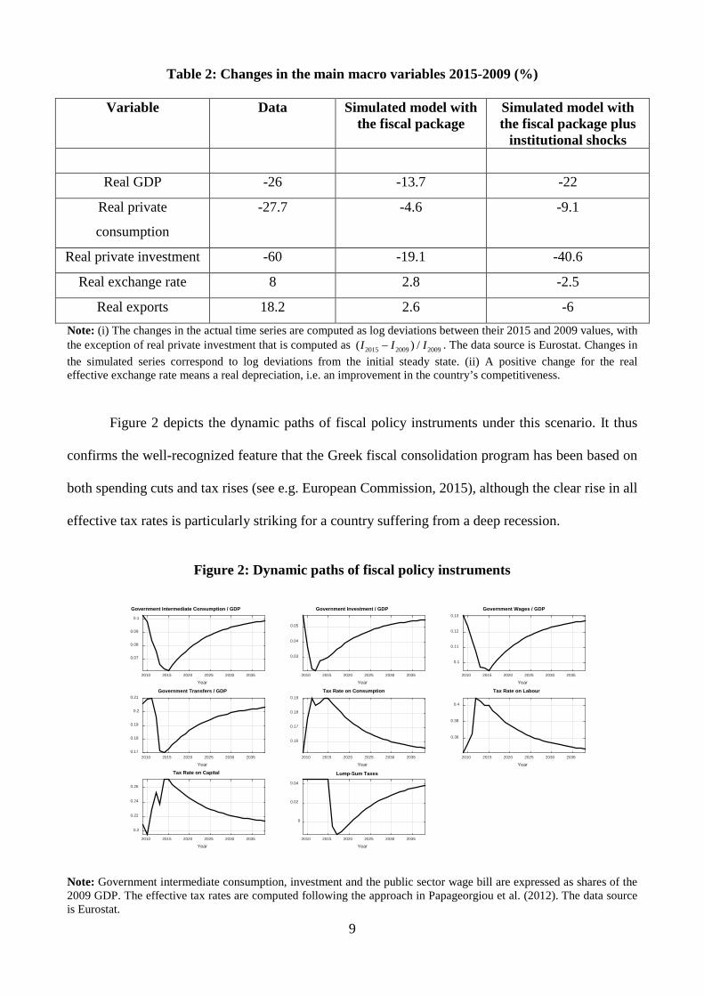
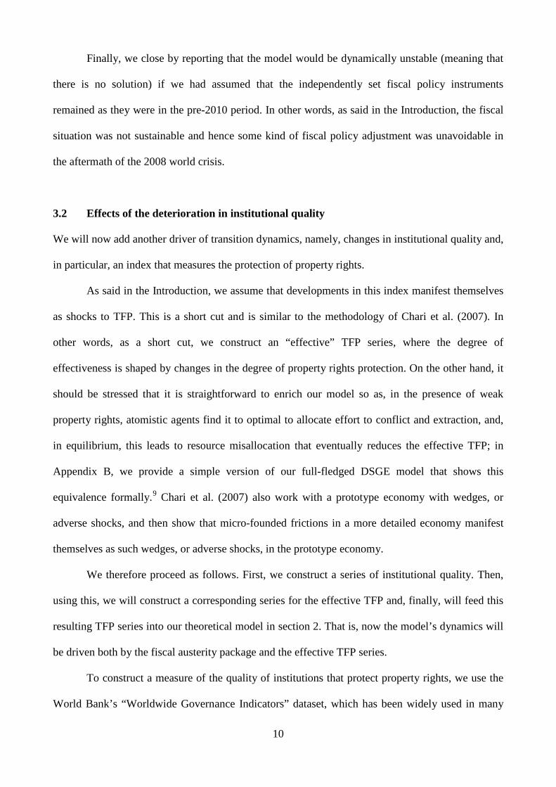
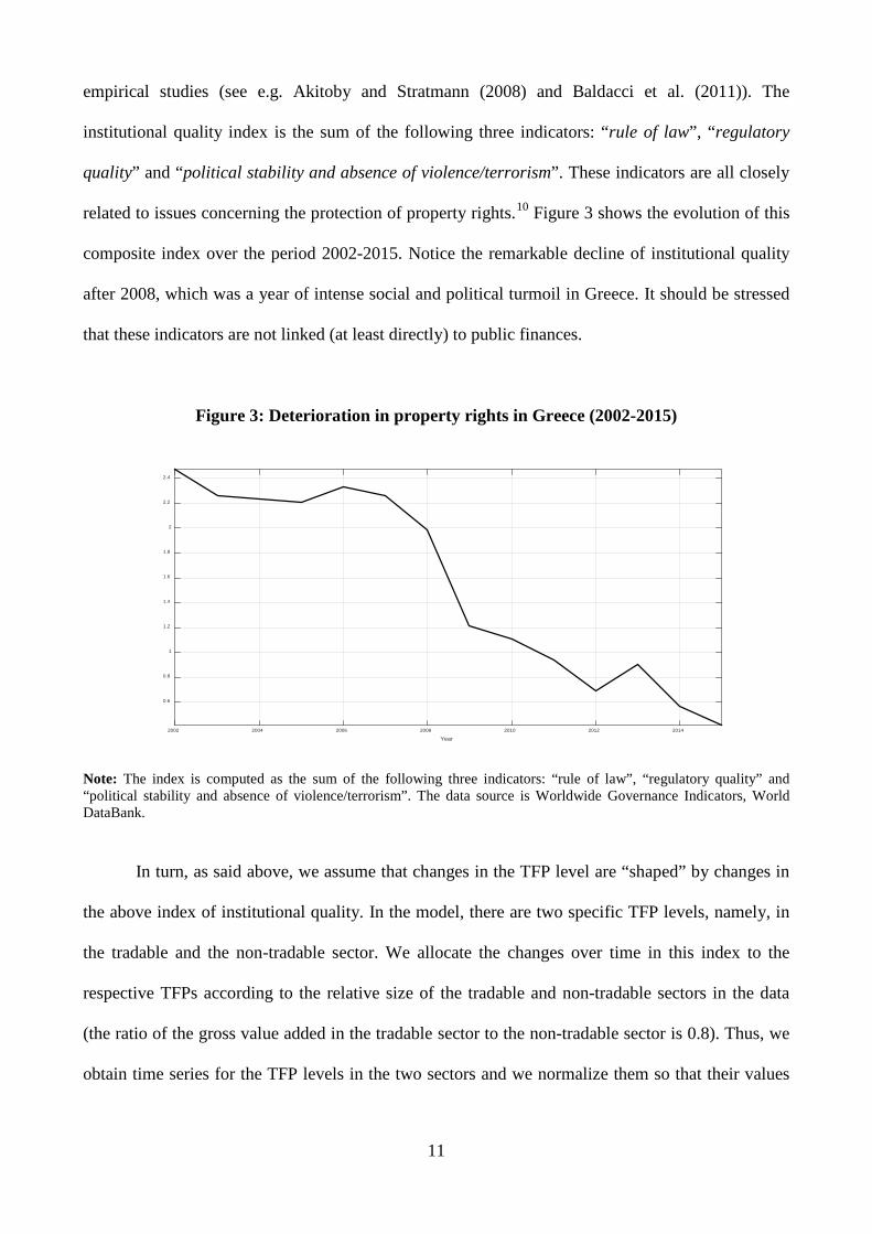
11

empirical studies (see eg Akitoby and Stratmann (2008) and Baldacci et al (2011)) The

institutional quality index is the sum of the following three indicators ldquorule of lawrdquo ldquoregulatory

qualityrdquo and ldquopolitical stability and absence of violenceterrorismrdquo These indicators are all closely

related to issues concerning the protection of property rights10 Figure 3 shows the evolution of this

composite index over the period 2002-2015 Notice the remarkable decline of institutional quality

after 2008 which was a year of intense social and political turmoil in Greece It should be stressed

that these indicators are not linked (at least directly) to public finances

Figure 3 Deterioration in property rights in Greece (2002-2015)

Note The index is computed as the sum of the following three indicators ldquorule of lawrdquo ldquoregulatory qualityrdquo and ldquopolitical stability and absence of violenceterrorismrdquo The data source is Worldwide Governance Indicators World DataBank

In turn as said above we assume that changes in the TFP level are ldquoshapedrdquo by changes in

the above index of institutional quality In the model there are two specific TFP levels namely in

the tradable and the non-tradable sector We allocate the changes over time in this index to the

respective TFPs according to the relative size of the tradable and non-tradable sectors in the data

(the ratio of the gross value added in the tradable sector to the non-tradable sector is 08) Thus we

obtain time series for the TFP levels in the two sectors and we normalize them so that their values

Year2002 2004 2006 2008 2010 2012 2014

06

08

1

12

14

16

18

2

22

24

12

in 2009 to be consistent with the calibrated values of the TFPs (equal to 1 for the non-tradable and

equal to 09241 for the tradable sector) Figure 4 shows the two constructed effective TFP series

Figure 4 TFP in tradable and non-tradable sectors

ldquoshapedrdquo by the deterioration in property rights

Note The path of the TFP levels is ldquoshapedrdquo by the changes in the institutional quality index according to the relative size of the respective sectors in the data Source Authorsrsquo calculations

Finally using all the above we repeat the same experiment as in section 31 by setting the

TFP levels of tradables and non-tradables over 2010-2015 equal to the constructed series The new

impulse response functions are plotted in Figure 5 while the last column in Table 2 which was

presented above summarizes the associated changes in the main macro variables Notice that now

the reduction in GDP in column 3 of Table 2 is 22 as compared to only 14 without the

TFPinstitutional shock in column 2

Year2009 2010 2011 2012 2013 2014 2015

085

09

095

1

105

TFP Tradable Sector

TFP Non-Tradable Sector

13

Figure 5 Impulse response functions driven by the fiscal austerity package and the deterioration in property rights

Note All variables are expressed as percentage deviations from the steady-state with the exception of the CPI inflation the interest rate foreign assets and the public debt-to-GDP ratio that are expressed as percentage point deviations

4 Conclusions discussion and extensions

In this paper we studied the quantitative importance of the fiscal austerity program and the

deterioration of institutional quality both as observed in the recent data for the Greek great

depression since 2010 The main result is that the adopted fiscal policy mix and the deterioration in

property rights are the main explanatory variables of the Greek great depression

We close with acknowledging two caveats First here we did not explain why the specific

fiscal policy mix has been chosen (which proves to be particularly distorting) or why the society has

chosen to have weak and deteriorating property rights (which leads to misallocation of resources

and hence to a relatively low TFP) In general it is well recognized that the policies chosen andor

the way resources are (mis)allocated are an equilibrium outcome of a political process interacting

with institutions and distribution (see eg Acemoglu (2009 chapter 4) and Jones (2011)) In the

case of Greece there is no shortage of conjectures about the root causes of such choices which go

back to the post-world war II history of the country Second our analysis here was only positive

One could search for instance for alternative fiscal policy mixes andor institutional regimes that

could perhaps mitigate the recessionary effects of debt consolidation We leave these extensions for

future research

Year2010 2020 2030 2040

D

evia

tion

-30

-20

-10

0Real Output

Year2010 2020 2030 2040

D

evia

tion

-15

-10

-5

0

5Domestic Tradable Output

Year2010 2020 2030 2040

D

evia

tion

-40

-30

-20

-10

0Non-Tradable Output

Year2010 2020 2030 2040

D

evia

tion

-60

-40

-20

0Consumption

TotalRicardianNon-Ricardian

Year2010 2020 2030 2040

D

evia

tion

-60

-40

-20

0

20Private Investment

Year2010 2020 2030 2040

D

evia

tion

-30

-20

-10

0Real Wages-Private Sector

2010 2020 2030 2040

P

oint

Dev

iatio

n

-2

0

2

4CPI Inflation

Year2010 2012 2014 2016 2018

P

oint

Dev

iatio

n

0

1

2

3Interest Rate

Year2010 2020 2030 2040

D

evia

tion

-10

-5

0

5Real Exchange Rate

Year2010 2020 2030 2040

D

evia

tion

-20

-10

0

10Trade Volumes

Exports

Imports

Year2010 2020 2030 2040

P

oint

Dev

iatio

n

-4

-2

0

2Foreign Assets

Year2010 2020 2030 2040

P

oint

Dev

iatio

n

-40

-20

0

20

40Public Debt GDP

14

References

Acemoglu D (2009) Modern Economic Growth Princeton University Press Princeton Anderson D Hunt B amp Snudden S (2014) Fiscal consolidation in the euro area How much pain can structural reforms ease Journal of Policy Modeling 36 785-799 Ardagna S (2001) Fiscal policy composition public debt and economic activity Public Choice 109 301-325 Akitoby B amp Stratmann T (2008) Fiscal policy and financial markets Economic Journal 118 1971-1985 Angelopoulos K Philippopoulos A amp Vassilatos V (2009) The social cost of rent seeking in Europe European Journal of Political Economy 25 280-299 Baldacci E Petrova I Belhocine N Dobrescu G amp Mazraani S (2011) Assessing fiscal stress IMF Working Papers WP11100 Washigton DC Bergoeing R Kehoe P Kehoe T and Soto R (2002) Policy driven productivity in Chile and Mexico in the 1980s and 1990s American Economic Review 92 16-21 Blanchard O amp Gali J (2007) Real wage rigidities and the new Keynesian model Journal of Money Credit and Banking 39 35-65 Cacciatore M Duval R amp Fiori G (2012) Short-term gain or pain A DSGE model based analysis of the short-term effects of structural reforms in labour and product markets OECD Economics Department Working Papers no 948 OECD Paris Calvo GA (1983) Staggered prices in a utility-maximizing framework Journal of Monetary Economics 12 383-398 Canova F (2007) Methods for Applied Macroeconomic Research Princeton University Press Princeton CESifo (2016) EEAG Report on the European Economy Munich Chari VV Kehoe P amp McGrattan E (2007) Business cycle accounting Econometrica 75 781-836 Christoffel K Coenen G amp Warne A (2008) The new area-wide model of the Euro area ndash A micro-founded open-economy model for forecasting and policy analysis European Central Bank Working Paper Series Number 944 Christoffel K amp Linzert T (2010) The role of real wage rigidities and labor market frictions for unemployment and inflation dynamics Journal of Money Credit and Banking 42 1435-1446 Christiano LJ amp Eichenbaum M (1992) Current real business cycle theories and aggregate labor market fluctuations American Economic Review 82 430-450 Christiano LJ Eichenbaum M amp Evans C (2005) Nominal rigidities and the dynamic effects of a shock to monetary policy Journal of Political Economy 113 1-45

15

Christiano LJ Trabandt M amp Walentin K (2011) DSGE models for monetary policy analysis In Friedman BM Woodford M (Eds) Handbook of Macroeconomics Volume 3 Elsevier North-Holland 285ndash367 Coenen G Mohr M amp Straub R (2008) Fiscal consolidation in the euro area long run benefits and short-run costs Economic Modeling 25 912-932 Coenen G Straub R amp Trabandt M (2013) Gauging the effects of fiscal stimulus packages in the euro area Journal of Economic Dynamics and Control 32 367-386 Corsetti G Kuester K Meier A amp Muller G (2013) Sovereign risk fiscal policy and macroeconomic stability Economic Journal 123 F99-F132 Duval R (2008) Is there a role for macroeconomic policy in fostering structural reforms Panel evidence for OECD countries over the past two decades European Journal of Political Economy 24 491-502 Economides G Park H amp Philippopoulos A (2007) Optimal protection of property rights in a general equilibrium model of growth Scandinavian Journal of Economics 109 153-175 Economides G Kalyvitis S amp Philippopoulos A (2008) Does foreign aid distort incentives and hurt growth Theory and evidence from 75 aid-recipient countries Public Choice 134 463-488 Economides G Papageorgiou D Philippopoulos A amp Vassilatos V (2013) Smaller public sectors in the Euro Area Aggregate and distributional implications CESifo Economic Studies 59 536-558 Eggertsson G Ferrero A amp Raffo A (2014) Can Structural reforms help Europe Journal of Monetary Economics 61 2-22 Erceg JC amp Linde J (2013) Fiscal consolidation in a currency union Spending cuts vs tax hikes Journal of Economic Dynamics and Control 37 422-445 European Commission (2010) The economic adjustment programme for Greece European Economy Occasional Papers Number 61 Brussels European Commission (2014) Public Finances in EMU Brussels European Commission (2015) Public Finances in EMU Brussels Forni L Monteforte L amp Sessa L (2009) The general equilibrium effects of fiscal policy estimates for the euro area Journal of Public Economics 93 559-585 Forni L Gerali A amp Pisani M (2010a) The macroeconomics of fiscal consolidations in euro area countries Journal of Economic Dynamics and Control 34 1791-1812 Forni L Gerali A amp Pisani M (2010b) Macroeconomic effects of greater competition in the service sector The case of Italy Macroeconomic Dynamics 14 677-708 Forni L amp Pissani M (2013) Macroeconomic effects of sovereign restructuring in a Monetary Union A model-based approach IMF Working Paper Number 13269

16

Gali J Lopez-Salido D amp Valles J (2007) Understanding the effects of government spending on consumption Journal of the European Economic Association 5 227-270 Garcia-Cicco J Pancrazi R amp Uribe M (2010) Real Business Cycles in Emerging Countries American Economic Review 100 2510-2531 Gerali A Notarpietro A and Pisani M (2014) Macroeconomic effects of simultaneous implementation of reforms after the crisis Bank of Italy Working Paper Number 997 Gerali A Notarpietro A amp Pisani M (2015) Structural reforms investment and zero lower bound in a monetary union Manchester School 83 120-139 Gogos S Mylonidis N Papageorgiou D amp Vassilatos V (2014) 1979-2001 A Greek great depression through the lens of neoclassical growth theory Economic Modelling 36 316-331 Gomes S Jacquinot P Mohr M amp Pisani M (2013) Structural reforms and macroeconomic performance in the euro area countries A model-based assessment International Finance 16 23- 44 Gourinchas P-O Philippon T amp Vayanos D (2016) The analytics of the Greek crisis Mimeo London School of Economics Hall R (2003) Wage determination and employment fluctuations NBER Working Paper Number 9967 Hall R (2005) Employment fluctuations with equilibrium wage stickiness American Economic Review 95 50-64 Heylen F Hoebeeck A amp Buyse T (2013) Government efficiency institutions and the effects of fiscal consolidation on public debt European Journal of Political Economy 31 40-59 IMF (2015a) Euro area policies 2015 Article IV consultation Country Report Number 15204 International Monetary Fund Washington IMF (2015b) Fiscal monitor - Now is the time Fiscal policies for sustainable growth International Monetary Fund Washington Jones C (2008) Macroeconomics Norton and Company New York Jones C (2011) Misallocation economic growth and input-output economics NBER Working Paper Number 16742 Kaufmann D Kraay A amp Mastruzzi M (2010) The worldwide government indicators Methodology and analytical issues World Bank Policy Research Working Papers Number 5430 Kehoe T amp Prescott E (2002) Great depressions of the 20th century Review of Economic Dynamics 5 1-18 Kliem M amp Uhlig H (2013) Bayesian estimation of a DSGE model with asset prices Deutsche Bundesbank Discussion Paper Number 372013

17

Malley J Philippopoulos A amp Woitek U (2009) To react or not Fiscal policy volatility and welfare in the EU-3 European Economic Review 53 689ndash714 Mendoza E (2010) Sudden stops financial crises and leverage American Economic Review 100 1941-1966 Mertens K amp Ravn M (2011) Understanding the aggregate effects of anticipated and unanticipated policy shocks Review of Economic Dynamics 14 27ndash54 OECD (2013) Economic Policy Reforms Going for Growth Paris OECD (2015) Economic Policy Reforms Going for growth Paris Papageorgiou D Efthimiadis T amp Konstantakopoulou I (2012) Effective tax rates in Greece Centre of Planning and Economic Research (KEPE) Discussion Paper Series Number 124 Papageorgiou D (2012) Fiscal policy reforms in general equilibrium the case of Greece Journal of Macroeconomics 34 504-522 Papageorgiou D (2014) BoGGEM A dynamic stochastic general equilibrium model for policy simulations Bank of Greece Working Paper Number 182 Papageorgiou D amp Vourvachaki E (2016) Macroeconomic effects of structural reforms and fiscal consolidations Trade-offs and complementarities European Journal of Political Economy Available from httpdxdoiorg101016jejpoleco201608010 Petrongolo B amp Pissarides C (2001) Looking into the black box A survey of the matching function Journal of Economic Literature 38 390-431 Philippopoulos A Vassilatos V and Varthalitis P (2016) Fiscal consolidation in an open economy with sovereign premia and without monetary policy independence International Journal of Central Banking forthcoming Prescott E (2002) Prosperity and depression American Economic Review 92 1-15 Roeger W amp in lsquot Veld J (2013) Expected sovereign defaults and fiscal consolidations European Economy Economic Papers no 479 Schmitt-Groheacute S amp Uribe M (2003) Closing small open economies Journal of International Economics 61 163-185 Schuknecht L von Hagen J amp Wolswijk G (2009) Government risk premiums in the bond market EMU and Canada European Journal of Political Economy 25 371-384 Stahler N amp Thomas C (2012) Fimod ndash A DSGE model for fiscal policy simulations Economic Modelling 29 239-261 Uhlig H (2007) Explaining asset prices with external habits and wage rigidities in a DSGE model American Economic Review 97 239-243 Vogel L (2012) Structural reforms fiscal consolidation and external rebalancing in monetary union A model-based analysis Economic Modelling 29 1286-1298

18

Vogel L (2014a) Nontradable sector reform and external rebalancing in monetary union A model-based analysis Economic Modelling 29 1286-1298 Vogel L (2014b) Structural reforms at the zero bound European Economy Economic Papers no 537

19

1 Namely the drop in output is large occurred rapidly and is sustained this is defined as a ldquogreat depressionrdquo See Gogos et al (2014) for an application of this methodology to the Greek economy before the euro period 2 There is a growing literature on the current Greek crisis For instance Bortz (2015) discusses where the financial assistance has gone offering a different view from that of Sinn (2015) Arellano and Bai (2016) study the Greek default Papageorgiou and Vourvachaki (2016) study the implications of structural reforms in light of the crisis Gourinchas et al (2016) search for shocks that can account for the Greek crisis See below for further details 3 See eg Philippopoulos et al (2016) for the different implications of different fiscal policy mixes used for debt consolidation in Italy 4 Alternatively we could for instance use a VAR approach which requires a limited amount of theory to structure the data (see eg Canova 2007 for methodology) We prefer to follow the DSGE approach so as to have well-defined micro-foundations that allow us to understand the behavioral channels through which exogenous changes affect macroeconomic outcomes 5 There is a large literature that shows how weak institutions affect the efficiency with which factor inputs are used and in particular how weak property rights lead to distortive individual incentives resource misallocation and eventually a lower level of total factor productivity See eg Jones (2008 chapter 4 and 2011) and Acemoglu (2009 chapter 4) for reviews of the literature while see below for further details and references Here working as in Chari et al (2007) we will take a short cut by assuming that changes in property rights directly show up as shocks to TFP nevertheless as argued in subsection 32 below this is equivalent to a richer model where the adverse effect of weak property rights on TFP works via the distortion of individual incentives 6 See eg Chari et al (2007) for a methodology paper on business cycle accounting 7 We focus on the period during which Greece is part of the euro area but before the debt crisis erupted in early 2010 8 In particular we assume that ( ) 1G H

t t tR mR m R= + minus where we set the value of m equal to 05

9 In the same spirit Economides et al (2007 2008) and Angelopoulos et al (2009 2012) also provide micro-founded dynamic general equilibrium models where the presence of weak property rights distorts private incentives and in equilibrium this leads to resource misallocation which in turn maps into reductions in the effective TFP All this belongs to a rich and still growing literature that endogenizes the TFP and hence endogenizes long-term growth 10 The rule of law indicator captures perceptions of the extent to which agents have confidence in and abide by the rules of society and in particular the quality of contract enforcement property rights the police and the courts as well as the likelihood of crime and violence The regulatory quality index captures perceptions of the ability of the government to formulate and implement sound policies and regulations and the credibility of governmentrsquos commitment to such policies The political stability and absence of violenceterrorism indicator captures perceptions of the likelihood that the government will be destabilized or overthrown by unconstitutional or violence means including politically-motivate violence and terrorism For further details see Kaufman et al (2010) We report that each one of these three sub-indexes is highly correlated with key macroeconomic variables such as real GDP and real investment in the Greek data

20

Appendix A A DSGE model and calibration

This appendix presents the model used It is similar to that in Papageorgiou (2014)

1 Households

The economy is populated by a continuum of households of mass one indexed by [ ]01hisin of

which a fraction indexed by [01 ]i λisin minus are referred as ldquoRicardianrdquo or ldquooptimizing householdsrdquo

and a fraction indexed by (1 1]j λisin minus are referred as ldquonon-Ricardianrdquo or ldquoliquidity constrained

householdsrdquo Optimizing households have access to capital and financial markets where they can

invest in the form of physical capital government bonds and internationally traded assets Liquidity

constrained households on the other hand are not able to lend or borrow so that they consume

their disposable labor income in each time period Both households supply differentiated labor

services and act as wage-setters in monopolistically competitive markets

11 Ricardian households

Ricardian households indexed by i have preferences over consumption and leisure The inter-

temporal utility function of each i is

( )10 0

Rt cti i t i t

tU E u C C Hβ ξ

infin

minus

=

= minussum (1)

where (01)β isin is the discount factor i tC is i rsquos effective consumption (defined below) at t i tH is

i rsquos total work hours at t [01)cξ isin is a parameter that measures the degree of external habit

formation in consumption and 1RtC minus denotes average (per household i ) lagged-once effective

consumption Effective consumption is in turn defined to be a linear combination of private

consumption p

i tC and public goods and services (education health etc) provided by the state

sector gtY 1

p g

i t i t tC C Yϑ= + (2)

where [ 11]ϑisin minus is the degree of substitutability between private and public consumption

The instantaneous utility function is assumed to be of the form

( ) ( )1

1 1 log

1

R R i tc ct ti t i t i t

Hu C C H C C

g

ξ ξ κg

+

minus minusminus = minus minus+

(3)

1 See eg Christiano and Eichenbaum (1992) Forni et al (2010a) and Economides et al (2013)

21

where g is the inverse of Frisch labour supply elasticity and 0κ gt is a preference parameter

related to work effort Each household i supplies work hours in the private sector p

i tH and the

public sector gi tH As in eg Ardagna (2001) and Forni et al (2009) hours of work can be moved

across the two sectors and are perfect substitutes in terms of (dis)utility so that p g

i t i t i tH H H= + in

each period t

The Ricardian household can save in the form of physical capital p

i tI domestic government

bonds i tB and foreign assets p

i tF It receives labour income from working in the private sector

p p

i t i tw H and the public sector g gi t i tw H where

pi tw and

gi tw are the real wage rates in the private and

public sector respectively The household rents out capital to firms and receives capital income

k p

t i t i tr u K where ktr is the real return to the effective amount of private capital

pi tK is the physical

private capital stock and 0i tu gt is the utilization rate of capital The household also earns interest

income from domestic government bonds and internationally traded assets that pay a gross nominal

interest 1tR ge and 1HtR ge at 1t + respectively In addition households own all domestic firms so

that they receive their profits as dividends i tDiv Finally each Ricardian household receives a

lump-sum government transfer tri tG The household pays taxes on consumption 0 1c

ttlt lt on

labour income 0 1lttlt lt on capital earnings and dividends 0 1k

ttlt lt and lump-sum taxes tT

Hence the budget constraint of each Ricardian household i is

( )

( )( ) ( )( )

1 1

1

1

1 1

pIi t t i tc p pt

t i t i tC C Ct t t

l p p g g k k pt i t i t i t i t t t i t i t i t

t

B S FPC IP P P

w H w H r u K Div

R

t

t t

+ +

minus

+ + + + =

= minus + + minus + +

+ 1

pi t t i tH tr h

t i t t i tC Ct t

B S FR G T

P Pminus+ + minus minusG

(4)

where CtP and I

tP are the prices of a unit of the private consumption final good and the investment

final good respectively and tS is the nominal exchange rate (expressed in terms of domestic

currency per unit of foreign currency) The household faces costs when it adjusts its private foreign

asset holdings hi tG whenever the private foreign assets-to-GDP ratio GDP

tY

t

ptit

YPFS 1 + deviates from its

long-run target level f In particular

( )2

1 1

2

pY GDPft i th p Y GDP C t t

i t t i t t t t C Y GDPt t t

S FP YS F P Y P fP P Y

ξ ++

G = minus

(5)

22

where GDPtY is the economyrsquos real GDP Y

tP is the GDP deflator and 0gefξ is an adjustment cost

parameter2

The private capital stock evolves over time according to the following law of motion

( )( ) 1

1

1 1p

i tp p p I pi t i t i t i tp

i t

IK u K I

Iδ+

minus

= minus + minusΨ

(6)

where IΨ is a convex adjustment cost function for investment as in eg Christiano et al (2005)

2

1 1

12

p pki t i tIp p

i t i t

I II I

ξ

minus minus

Ψ = minus

(7)

where (1) (1) 0I IΨ = Ψ = and 0kξ ge is an adjustment cost parameter We assume that the

depreciation rate of private capital depends on the rate of capacity utilization and is a convex

function that satisfies 0pδ prime gt 0pδ primeprime gt so that ( ) p p

i t i tu uϕδ δ= where (01)pδ isin and 0ϕ gt are

respectively the average rate of depreciation of private capital and the elasticity of marginal

depreciation cost

The first-order conditions of this problem are written below when we present the final

equilibrium system

12 Non-Ricardian households

Liquidity constrained households indexed by j have the same preferences as Ricardian

households They receive labour income from working in the private and public sectors but have no

access to capital or financial markets so that in each period their consumption spending equals

their after-tax wage income plus lump-sum government transfers The period-by-period budget

constraint of each household j is

( ) ( )( ) 1 1c l p p g g trt j t t j t j t j t j t j tC w H w H Gt t+ = minus + + (8)

where pj tH and

gj tH are respectively hours worked in the private and public sector by household j

and trj tG is a lump-sum government transfer to each j Thus as in eg Coenen et al (2013) we

allow for a potentially uneven distribution of government transfers across Ricardian and non-

Ricardian households

The first-order conditions of this problem are written below when we present the final

equilibrium system

2 This specification ensures that foreign private assets are stationary see eg Schmitt-Grohe and Uribe (2003)

23

2 Wage setting and the evolution of wages in the private sector

We assume that wages in the private sector are set by monopolistic unions as in eg Forni et al

(2009) and Gali et al (2007) More specifically households supply differentiated labour varieties to

a continuum of unions [ ]01hisin each of which represents a specific labour variety Every variety is

uniformly distributed across households so that each union ultimately represents 1 λminus fraction of

Ricardian households and λ of non-Ricardian households In every period each union sets the

wage rate for its own workers by trading off the utility derived from private sector labour income

and the disutility of total work effort by taking into account the demand for the differentiated labour

variety h At the same time private and public sector firms allocate their labour demand uniformly

across the h labour varieties independently of the type of households which implies that hours

worked by each type of household are equal

h p h p pj t i t h tH H H= equiv and

h g h g gj t i t h tH H H= equiv 3

Therefore in each period a typical union h chooses the wage rate ph tw to maximize

( ) ( ) ( )1

1 1 1

1h tNR l p p R l p p

w h t h t h t h t h t h t

HL w H w H

g

λ t λ t κg

+

= L minus + minus L minus minus + (9a)

subject to

1

Wt

Wt

ph tp p

h t tpt

wH H

w

micromicro

minusminus

=

(9b)

p g

h t h t h tH H H= + (9c)

where Eq (9b) is the demand for the differentiated labour input h ptH is total labour demand in the

private sector ptw is the aggregate wage rate in the private sector and

NRh tL

Rh tL are the marginal

utilities of consumption of non-Ricardian and Ricardian households of labour variety h

respectively used as weights Finally ( ) 1 1W Wt tmicro micro minus gt is the elasticity of substitution across the

differentiated labour services where 1Wtmicro gt is the wage markup in the private labour market

Focusing on a symmetric equilibrium in which all unions choose the same wage rate ex

post the first-order condition of the above problem is

1p Wt tNR R

t t

wMRS MRS

λ λ micro minus

+ =

(10)

3 Total public sector labour demand for the differentiated labour input ℎ is exogenous and is defined as 1

0

g gt h tH H dh= int

24

where ptw is the optimal wage rate chosen by unions and NR

tMRS and RtMRS are the marginal

rates of substitution between consumption and leisure of non-Ricardian and Ricardian households

respectively4

Following eg Hall (2005) and Blanchard and Gali (2007) we introduce further rigidities in

the labour market by assuming that real wages respond sluggishly to labour market conditions In

particular the real wage rate in the private sector is modeled as a weighted average of the lagged-

once real wage rate and the optimal real wage rate chosen by unions

( ) ( )11

n np p pt t tw w w

minus

minus= (11)

where 0 1nle le denotes the degree of real wage rigidities and ptw is given by (10)5 This

formulation aims to capture the rigidities found in the Greek labour market (see eg the discussion

in European Commission 2010)6

3 Production in the private sector

There are two types of domestic firms The first type consists of monopolistically competitive firms

that produce intermediate goods tradable and non-tradable The continuum of firms producing

differentiated varieties of tradables indexed by [ ]01Tf isin sell their output domestically or abroad

(the latter are recorded as exports) The continuum of firms producing differentiated varieties of

non-tradables indexed by [ ]01Nf isin sell their output domestically only There is also a continuum

of monopolistically competitive firms importing intermediate goods indexed by [ ]01Mf isin The

second type of firms consists of four perfectly competitive firms that produce final goods These

firms combine purchases of intermediate goods to produce four non-tradable goods a private

consumption good a private investment good a public consumption good and a public investment

good Finally there is a foreign final goods firm that combines purchases of the exported domestic

intermediate goods

4 Note that when 0λ = ie when all households are Ricardian W

tmicro reduces to a markup of the optimally chosen real

wage rate over the marginal rate of substitution between consumption and leisure of Ricardian households 5 See also eg Uhlig (2007) Malley et al (2009) and Kliem and Uhlig (2013) for a similar specification Microfoundations for Eq (11) can be found in eg Hall (2003) Petrongolo and Pissarides (2001) and Christoffel and Linzert (2010) 6 Papageorgiou (2014) finds that this specification can capture rather well the aggregate dynamics of work hours and real wages in Greece

25

31 Final goods firms

As said above there are four representative final goods firms that combine purchases of tradable

intermediate goods with non-tradable goods to produce a private consumption good ptC a private

investment good ItI a public consumption good gc

tG and a public investment good gitG

Private consumption goods producer

The representative producer of the private final consumption good combines a bundle of tradable

consumption intermediate goods TtC with a bundle of non-tradable intermediate goods N

tC

according to a constant elasticity of substitution (CES) production function

( ) ( )1 11 1 1

(1 )

C

C C CC CC C

p T Nt C t C tC C C

εε ε ε

ε εε εω ωminus minus minus

= + minus

(12)

where [ ]01Cω isin measures the weight of tradable goods in the production of the final private

consumption good and 0Cε gt is the elasticity of substitution between tradable and non-tradable

consumption goods

In turn the tradable intermediate consumption good bundle is a CES function of the

domestically produced bundle of tradable intermediate consumption goods DtC and the bundle of

imported intermediate consumption goods MtC

( ) ( )1 11 1 1

(1 )

TC

TC TC TCTC TCTC TC

T D Mt TC t TC tC C C

εε ε ε

ε εε εω ωminus minus minus

= + minus

(13)

where [ ]10isinTCω measures the home bias in the production of the tradable intermediate

consumption good and 0TCε gt is the elasticity of substitution between domestic and imported

intermediate consumption goods

The intermediate consumption good bundles that are used as inputs combine differentiated

varieties supplied by intermediate good firms Specifically the varieties supplied by each tradable

intermediate goods firm Tf T

Df t

C each non-tradable intermediate-goods firm Nf N

Nf t

C and each

importing firm Mf M

Mf t

C are respectively combined using a CES technology into

( )1

1

0

Tt

Tt

TD D Tt f t

C C dfmicro

micro

= int (14a)

26

( )1

1

0

Nt

Nt

NN N Nt f t

C C dfmicro

micro

= int (14b)

( )1

1

0

Mt

Mt

MM M Mt f t

C C dfmicro

micro

= int (14c)

where 1T N Mt t tmicro micro micro gt are the intra-temporal elasticities of substitution between different varieties

within each type of intermediate consumption good As we show below T N Mt t tmicro micro micro represent

markups in the markets of domestic and imported intermediate goods

Given the above technology the producer of the final private consumption good solves a

three stage problem In the first stage it takes as given the prices of domestic tradable N

Df t

P non-

tradable T

Nf t

P and imported intermediate goods M

Mf t

P and chooses the amounts of the

differentiated goods T

Df t

C N

Nf t

C M

Mf t

C in order to minimize total expenditures for the bundles of

the differentiated goods 1

0

T TD D Tf t f t

P C dfint 1

0

N NN N Nf t f t

P C dfint 1

0

M MM M Mf t f t

P C dfint subject to the aggregation

constraints in (14a)-(14c) The solution of the cost minimization problem gives the demand

functions for these intermediate goods Tf Nf and Mf respectively

1

Dt

DtT

T

Df tD D

tDf tt

PC C

P

micromicro

minusminus

=

(15a)

1

Nt

NtN

N

Nf tN N

tNf tt

PC C

P

micromicro

minusminus

=

(15b)

1

Mt

MtM

T

Mf tM M

tMf tt

PC C

P

micromicro

minusminus

=

(15c)

where D N Mt t tP P P are the aggregate price indices of domestic tradable non-tradable and imported

intermediate consumption goods respectively

In the second stage the firm chooses the bundles DtC and M

tC in order to maximize its

profits 1C TC T D D M Mt t t t t t tP C P C P CP = minus minus subject to the technology constraint (13) and by taking as

given the price indexes of domestic tradables TCtP non-tradables D

tP and imported intermediate

consumption goods MtP Thus it solves

27

max

D Mt t

TC T D D M Mt t t t t t

C CP C P C P Cminus minus

subject to

( ) ( )1 11 1 1

(1 )

TC

TC TC TCTC TCTC TC

T D Mt TC t TC tC C C

εε ε ε

ε εε εω ωminus minus minus

= + minus

In the third stage the firm chooses the demand for TtC and N

tC to maximize profits

2C C C TC T N Nt t t t t t tP C P C P CP = minus minus subject to the technology constraint (12) and by taking the input

prices CtP TC

tP and NtP as given Thus it solves

max

T Nt t

C C TC T N Nt t t t t t

C CP C P C P Cminus minus

subject to

( ) ( )1 11 1 1

(1 )

C

C C CC CC C

p T Nt C t C tC C C

εε ε ε

ε εε εω ωminus minus minus

= + minus

The demand functions for domestic tradable and imported consumption goods as well as for

tradable and non-tradable intermediate consumption goods resulting from the optimization problem

of the final consumption good firm are

TCD Dt t

TCT TCt t

C PC P

ε

ωminus

=

(16a)

( )1TCM M

t tTCT TC

t t

C PC P

ε

ωminus

= minus

(16b)

CT TCt t

CC Ct t

C PC P

ε

ωminus

=

(16c)

( )1CN N

t tCC C

t t

C PC P

ε

ωminus

= minus

(16d)

From the zero profit condition we get the price index for tradable consumption goods

( ) ( )( )1

1 1 11TC TC TCTC D M

t TC t TC tP P Pε ε εω ω

minus minus minus = + minus and the price index of a unit of the final consumption

good (ie the Consumption Price Index) ( ) ( ) ( )1

1 1 11C C CC TC N

t C t C tP P Pε ε εω ω

minus minus minus = + minus where

D N Mt t tP P P are the prices of domestic tradable intermediates non-tradable intermediates and

imported intermediate goods respectively

28

Private investment goods producer

Optimal decisions regarding the production of the final private investment good are derived in an

analogous manner as above The representative producer of the private investment good combines a

composite bundle of tradable intermediate goods TtI with a bundle of non-tradable intermediate

goods NtI to generate a composite final private investment good I

tI by using a constant elasticity

of substitution (CES) production function

( ) ( )1 11 1 1

(1 )

I

I I II II I

I T Nt I t I tI I I

εε ε ε

ε εε εω ωminus minus minus

= + minus

where [ ]01Iω isin measures the weight of tradable goods in the production of the final private

investment good and 0Iε gt is the elasticity of substitution between tradable and non-tradable

investment goods

In turn the composite bundle of the tradable intermediate investment good that is used in the

production of final investment goods is a CES function of domestically produced tradable

intermediate investment goods DtI and imported intermediate investment goods M

tI

( ) ( )1 1 11 1

(1 )

TI

TITI TITI TITI TI

T D Mt TI t TI tI I I

εεε ε

ε εε εω ωminusminus minus

= + minus

where [ ]01TIω isin measures the home bias in the production of the tradable intermediate

consumption good and 0TIε gt is the elasticity of substitution between domestic and imported

investment goods

The demand functions for domestic tradable and imported investment goods as well as for

tradable and non-tradable investment goods are

TID Dt t

TIT TIt t

I PI P

ε

ωminus

=

( )1TIM M

t tTIT TI

t t

I PI P

ε

ωminus

= minus

IT TIt t

II It t

I PI P

ε

ωminus

=

( )1IN N

t tIT I

t t

I PI P

ε

ωminus

= minus

29

where ( ) ( )( )1

1 1 11TI TI TITI D M

t TI t TI tP P Pε ε εω ω

minus minus minus = + minus and ( ) ( )( )

11 1 11

I I II TI Nt I t I tP P P

ε ε εω ωminus minus minus = + minus

are respectively the price indices for tradable intermediate investment goods and final investment

goods

Public consumption and investment goods production

Regarding the final public consumption and investment goods gctG and gi

tG we assume they are

produced using only non-tradable intermediate goods Hence gc Nt tG GC= and gi N

t tG GI= where

( )1

1

0

Nt

Nt

NN N Nt f t

GC GC dfmicro

micro

= int and ( )

11

0

Nt

Nt

NN N Nt f t

GI GI dfmicro

micro

= int

The optimal demand functions are

1

Nt

NtN

N

Nf tN N

tNf tt

PGC GC

P

micromicro

minusminus

=

and 1

Nt

NtN

N

Nf tN N

tNf tt

PGI GI

P

micromicro

minusminus

=

Aggregating across final good producing firms we get the respective aggregate domestic demand

functions for non-tradable domestic tradable and imported intermediate goods Tf Nf and mf

1

Nt

NtN

N N N N N

Nf tNT N N N N NT

tNf t f t f t f t f tt

PY C I GC GI Y

P

micromicro

minusminus

= + + + =

1

Tt

TtT

T T T

Df tD D D D

tDf t f t f tt

PY C I Y

P

micromicro

minusminus

= + =

1

Mt

MtM

M M M

mf tM M M M

tmf t f t f tt

PY C I Y

P

micromicro

minusminus

= + =

where NT N N N Nt t t t tY C I GC GI= + + + D D D

t t tY C I= + and M M Mt t tY C I= + are respectively the total

demand for non-tradable goods total domestic demand for domestically produced tradable goods

and total demand for imports

32 Intermediate goods firms

Each tradable and non-tradable intermediate good Tf t

Y and Nf t

Y is produced by a continuum of

monopolistically competitive intermediate goods firms indexed by [ ]01Tf isin and [ ]01Nf isin

respectively according to the production technologies

30

( ) ( ) ( )1

T T G

T T T

a a aT gt t Tf t f t f t

Y A K H Kminus

= minusΦ (17a)

( ) ( ) ( )1

N N G

N N N

a a aN gt t Nf t f t f t

Y A K H Kminus

= minusΦ (17b)

where Tf t

K is private capital Tf t

H is work hours in the private sector gtK is public capital

0T Na a gt are the output elasticities of capital services in the tradable and non-tradable sectors

respectively and 0Ga gt is the output elasticity of public capital7 Finally 0T NΦ Φ ge are fixed

costs of production and TtA N

tA are sector-specific total factor productivity levels

Tradable sector

In what follows we present the problem of intermediate goods firms in the tradable sector

Domestic intermediate goods firms in the tradable sector solve a two-stage problem In the first

stage each firm takes as given factor prices ktr and p

tw and chooses capital and labour inputs

Tf tK and

Tf tH in order to minimize total real input cost We also introduce a working capital

channel in the form of a ldquocash-in-advancerdquo constraint in the spirit of eg Mendoza (2010) In

particular at the beginning of each period each firm borrows from international lenders in order to

cover a fraction (01)tv isin of their total labour costs in advance of revenuesrsquo receipt The working

capital loan is repaid by the end of the period at the domestic country gross interest rate HtR Thus

the intratemporal problem of each firm involves the minimization of their costs inclusive of the

costs of serving their intra-period working capital loan In other words

( )

min 1T T TT Tf t f t

k p H pt t t t tf t f t f tK H

r K w H R v w H+ + minus (18)

subject to (17a)

The first-order conditions are

( )( ) ( )

1 1 1T

T

T

Tf tH pt t t T f t

f t

YR w a mc

Hν

+Φ+ minus = minus (19)

T

T

T

Tf tkt T f t

f t

Yr a mc

H

+Φ= (20)

where Tf t

mc is the Lagrange multiplier associated with the technology constraint that is the real

marginal cost in terms of the consumer prices CtP Because firms borrow to cover part of their

7 These production functions have increasing returns to scale with respect to all inputs and constant returns to scale with respect to private inputs (see also eg Baxter and King (1993) and Leeper et al (2010))

31

labour costs the marginal cost of labour is higher than the wage rate in the private sector As a

result increases in either the share of labour costs that are financed through working capital loans

or in the domestic interest rate directly increase the cost of labour and thereby reduce labour

demand

The labour input Tf t

H is a composite aggregate of household-specific varieties T

hf t

H

( )1

1

0

Wt

Wt

T Th

f t f tH H

micro

micro

= int Optimal demand is

1

Wt

T T

ph thpf t f t

t

wH H

w

micro =

where ( 1) 1W Wt tmicro micro minus gt is the

elasticity of substitution across differentiated labour services and ptw is the aggregate real wage

index in the private sector that is given by ( )11

1 10

Wt

Wtp p

t h tw wmicro

micro

minus

minus

= int

In the second stage intermediate good firms in the tradable sector choose the price that

maximizes discounted real profits As in Christoffel et al (2008) firms charge different prices at

home and abroad setting prices in producer currency In both domestic and foreign markets we

assume that prices are sticky aacute la Calvo (1983) In particular each period t the firm Tf optimally

resets prices with a constant probability 1 Dpθminus when it sells its differentiated product in the

domestic market and with probability 1 Xpθminus when it sells its product abroad The firms that cannot

optimize partially index their prices to aggregate past inflation according to the price indexation

schemes ( )1 1

D

T T

xD D Dtf t f t

P P minusminus= P and ( )1 1

X

T T

xX X Xtf t f t

P P minusminus= P where

TDf t

P denote the domestic price of

good Tf T

Xf t

P its foreign price and 1D D Dt t tP PminusP = 1X X X

t t tP PminusP = where D Xt tP P are the

aggregate domestic and export price indices (defined below) respectively The indexation

parameters [ ] 01D Xx x isin determine the weights given to past inflation

Each firm Tf which can optimally reset its price in period t knows with probability Dpθ

that this price will continue to be in effect t periods ahead and so chooses the optimal price

TD

f tP

to maximize the discounted sum of expected real profits (in terms of consumer prices CtP ) by

taking aggregate domestic demand DtY and the aggregate price index in the domestic market D

tP

as given Thus each firm Tf maximizes

( ) ( )

1

0 1

maxTD

TDTf t

DR Dx f tD D D Dt tt p t s tR D Df tP st t t

P PE mc YP P

t tt t

t tt t t

βθinfin

+ ++ minus + +

= = + +

L P minus L sum prod (21)

32

subject to

( )1

1

1

Tt

TtTD

T

Dx f tD D D

t s tDf ts t

PY Y

P

t

t

micromicrot

tt

+

+

minusminus

+ minus += +

= P prod (22)

where D C T Dt t t tmc P mc P= is the real marginal cost in terms of the domestic price index and

R Rt tt+L L is the ratio of the marginal utilities of consumption of Ricardian households - that are the

owners of the firms - according to which firms value future profits8 Notice that since all firms face

the same marginal cost and take aggregate variables as given any firm that optimizes will set the

same price

TD D

tf tP P=

Thus the first-order condition of the above problem is

( ) ( ) ( )1

1 1

1 1

0

Tt

TD Dtx xD DR D D D

t s t sD D T Dt t t tt p t t tR D D D D D

s st t s t t t s t

P P PE Y mcP P P

t

t

micromicro

t tt t tt t t

t

βθ micro

+

+

minusminus

+ minus + minus+ ++ + +

= =+ + +

P PL minus = L P P

prod prod (23)

According to the above expression firms set nominal prices so as to equate the average future

expected marginal revenues to average future expected marginal costs9 The aggregate domestic

index evolves according to ( )( ) ( )( )111

1 11 11

Tt

TDT ttxD D D D D D

t p t p t tP P Pmicro

micromicroθ θ

minus

minusminusminus minus

= minus + P

Similarly the associated first-order condition of each firm Tf that chooses its price in the

foreign market in period t is

( ) ( ) ( )1

1 1

1 1

0

Xt

XX Xtx xX XR X X X

t s t sX X X Xt t t tt p t t tR X X C X X

s st t s t t t s t

P P PE Y mcP P P

t

t

micromicro

t tt t tt t t

t

βθ micro

+

+

minusminus

+ minus + minus+ ++ + +

= =+ + +

P PL minus = L P P

prod prod (24)

where X C T Xt t t tmc P mc P= is the real marginal cost in terms of the aggregate export price index and

the aggregate export price index is ( )( ) ( )( )111

1 11 11

Xt

XXx ttxX X X X X X

t p t p t tP P Pmicro

micromicroθ θ

minus

minusminusminus minus

= minus + P

8 In equilibrium the marginal utility of consumption is common across Ricardian households

Ri t tL = L

9 In the case of fully flexible prices 0Dpθ = the above condition reduces to the static relation D T C T

t t t tP P mct tmicro + +=

which states that the price is equal to a markup over the nominal marginal cost

33

Non-tradable sector

The optimal demand by each firm Nf for labour of type h is

1

Wt

Wt

N N

ph thpf t f t

t

wH H

w

micromicro

minusminus

=

and the

aggregate demand for labour of type h is

11

0

Wt

Wt

N

ph tN h N

h t tpf tt

wH H df H

w

micromicro

minusminus

= =

int where NtH is total

labour demand in the non-tradable intermediate good sector As in the case of the tradable good

firms non-tradable intermediate good firms take short-term loans from international lenders at the

home countryrsquos gross interest rate HtR in order to finance a fraction tv of their total labour costs

To minimize costs each firm takes as given the factor prices ktr and p

tw and chooses N Nf t f t

K H

in order to minimize total real input cost ( ) 1N N N

k p H pt t t t tf t f t f t

r K w H R v w H+ + minus subject to the

production function The first-order conditions are

( )( ) ( )

1 1 1N

N

N

Nf tH pt t t N f t

f t

Yv R w a mc

H

+Φ+ minus = minus

N

N

N

Tf tkt N f t

f t

Yr a mc

K+Φ

=

where due to symmetry N

Ntf t

mc mc=

Non-tradable intermediate good firms face price stickiness aacute la Calvo with 1 Npθminus being the

probability that a firm Nf can optimally reset its price in any given period 0t ge The optimal

pricing is characterized by the following conditions

( ) ( ) ( )1

1 1

1 1

0

Nt

Nd Ntx xN NR N N N

t s t sN N N Nt t t tt p t t tR N N C N N

s st t s t t t s t

P P PE Y mcP P P

t

t

micromicro

t tt t tt t t

t

βθ micro

+

+

minusminus

+ minus + minus+ ++ + +

= =+ + +

P PL minus = L P P

prod prod

and the aggregate domestic index evolves according to

( )( ) ( )( )111

1 11 11

Nt

NNN ttxN N N N N N

t p t p t tP P Pmicro

micromicroθ θ

minus

minusminusminus minus

= minus + P

Importing firms

There is a continuum of importing firms [ ]01Mf isin each of which imports a single differentiated

intermediate good M

Mf t

Y These firms operate under monopolistic competition so that they have

34

pricing power This creates a wedge between the price at which the importing firms buy the foreign

differentiated goods in the world markets Yt tS P and the price at which they sell these goods to

domestic households M

Mf t

P Importing firms face price stickiness aacute la Calvo with 1 Mpθminus being the

probability that a firm Mf can optimally reset its price in the domestic market in any given period

0t ge so that optimal pricing follows

( ) ( ) ( )1

1 1

1 1

0

Mt

Mm mtx xM MR M M M

t s t sm M M Mt t t tt p t t tR M M C M M

s st t s t t t s t

P P PE Y mcP P P

t

t

micromicro

t tt t tt t t

t

βθ micro

+

+

minusminus

+ minus + minus+ ++ + +

= =+ + +

P PL minus = L P P

prod prod

and the aggregate import price index evolves according to

( )( ) ( )( )111

1 11 11

Mt

MmM ttxM m M m M M

t p t p t tP P Pmicro

micromicroθ θ

minus

minusminusminus minus

= minus + P

33 Demand from foreign final goods firms

We now model the demand coming from foreign firms or equivalently specify the domestic

countryrsquos exports Recall that the domestic economy produces intermediate tradable goods that are

also exported and so we need to model a final goods firm that transforms them into final goods

There is a representative foreign final good firm that purchases the differentiated exported goods

X

f tY produced by the domestic tradable intermediate good firms Tf and transforms them into a

homogeneous final good XtY via the CES technology

( )1

11

0

XtX

tT

X X Tt f t

Y Y dfmicro

micro

= int (25)

where 1Xtmicro gt is related to the intratemporal elasticity of substitution between the differentiated

outputs supplied by domestic intermediate good firms ( ) 1 1X Xt tmicro micro minus gt

The foreign firm takes the prices of exported differentiated goods

TX

tf tP S (expressed in

terms of the foreign currency) as given and chooses the optimal amounts of differentiated inputs to

minimize total input costs ( )1

0T T

X X Ttf t f t

P S Y dfint subject to (25) so that the optimal demand function

for each input T

Xf t

Y is 1

Xt

XtT

T

Xf tX X

tXf tt

PY Y

P

micromicro

minusminus

=

where ( )11

11

0

Xt

Xt

TX X T

t f tP P df

micro

micro

minus

minus

= int is the aggregate

price index of exported domestic intermediate goods and XtY is total foreign demand for domestic

35

intermediate goods The latter is

XX

X t tt tX

t

P SY YP

εminus

=

where X

tP is the price of foreign

competitors in the export markets tY is foreign economy output and 0Xε gt is the price elasticity

of export demand

4 The public sector

We now model the public sector

41 Government budget constraint and fiscal policy instruments

The government levies taxes on consumption labour income capital earnings and dividends We

also assume lump-sum taxestransfers The government also sells one-period government bonds to

the domestic bond market 1gtB + and the international market 1

gtF + Total tax revenues plus the issue

of new government bonds are used to finance government consumption ctG investment i

tG

transfers trtG and the wage bill of public sector employees g g

t tw H Moreover the interest rates

that the government pays on inherited domestic public debt and on foreign public debt are tR and

GtR respectively We assume that G

tR is a weighted average of the market interest rate that the

country faces when it borrows from abroad and the risk-free world interest rate (see below for

details) Thus the within-period government budget constraint in per-capita terms is

( ) ( )1 1

1 1

g gc p l p p g g k k pt t tt t t t t t t t t t t t tc C

t tN N g g

c i tr g g Gt t t t tt t t t t t tC C C C

t t t t

B S F C w H w H r u K Div TP P

P P B S FG G G w H R RP P P P

t t t+ +

minus minus

+ + + + + + + =

= + + + + +

(26)

Therefore the government has eleven policy instruments 1 1 c l k g g c i tr g gt t t t t t t t t t t tX T w H G G G B Ft t t + +isin

out of which ten can be exogenously set

To ensure dynamic stability we need to assume that one of the exogenously set fiscal policy

instruments follows a state-contingent rule reacting systematically to deviations of the public debt-

to-GDP ratio from a target level and the rate of change of debt

( ) ( )1 1 2 1d y d y y

t t t t tX X D d D Dφ φminus minus= + minus + minus (27)

where 1 1

y tt y GDP

t t

DDP Yminus minus

equiv denotes the debt-to-GDP ratio in the beginning of period t d is a target value

of the public debt-to-GDP ratio (see below for details) and 1 2 0d dφ φ gt are feedback policy reaction

coefficients (as in a Taylor rule for the nominal interest rate)

36

For notational convenience we will define the share of total public debt held by domestic

agents at the end of period t as 1

1

gt

tt

BD

ζ +

+

equiv where 0 1tζle le so that 1 1(1 )gt t t tS F Dζ+ += minus and

1 1 1g g

t t t tD B S F+ + += +

42 Production of public goodsservices

On the production side following eg Forni et al (2010a) and Economides et al (2013 2016) we

assume that the government combines public spending on goods and services ctG and public

employment gtH to produce public goodsservices g

tY according to the production function

( ) ( )1g c gt t t tY A G H

c cminus= (28)

where 0 1cle le is a technology parameter

The law of motion of public capital in per-capita terms is

( )1 1g g g it t tK K Gδ+ = minus + (29)

where ( )01gδ isin is the depreciation rate of public capital stock and 0 0gK gt is given

Regarding the inputs used in the above production function ctG is produced by final good

firms that use only non-tradable intermediate goods as inputs (see above) while gtH is total public

sector demand for the differentiated labour variety h that is exogenous (see above)

5 World capital markets and sovereign spreads

Following most of the literature on small open economies we assume that when domestic

households and the government participate in the world capital market they face an interest rate

that is public debt elastic (see eg Schmitt-Grohe and Uribe 2003)

In particular the nominal interest rate at which the country borrows from the international

market HtR bears a risk-premium term 0tψ ge that introduces a wedge between the interest rate

that the home country faces and the risk-free world nominal interest rate tR

max Ht t t tR R Rψ= + (30)

where as in eg Christiano et al (2011) Garcia-Cicco et al (2010) and Philippopoulos et al

(2016) the risk-premium is assumed to be an increasing function of public debt imbalances

( )( )1exp 1d yt tD dψ ψ += minus minus (31)

where 0dψ ge is a risk parameter and 0d gt is an exogenous threshold above which premia

emerge Thus when the public debt-to-GDP ratio is above a threshold level an interest rate spread

37

arises which is consistent with empirical evidence (see eg Ardagna et al 2008 Roeger and inrsquot

Veld 2013 Schuknecht et al 2009 Corsetti et al 2013) Conceptually the risk premium

component on the right hand side of (31) reflects the risk of sovereign or country default and thus

provides a channel through which such a risk affects directly the real economy

6 Monetary-exchange rate policy regime

We model the domestic economy as a member of a currency union in the sense that the nominal

exchange rate tS is exogenously set and at the same time there is no monetary policy

independence The latter means that the domestic nominal interest rate on government bonds tR is

determined endogenously (see eg Philippopoulos et al (2016) for details)

7 Aggregation and market-clearing conditions

71 Aggregation

The aggregate quantity expressed in per-capita terms of any household specific variable h tX is

given by ( )1

01t h t i t j tX X dh X Xλ λ= = minus +int Thus per capita private consumption is given by

( ) 1p p pt i t j tC C Cλ λ= minus + Since only optimizing households have access to the capital bond

dividend and international markets the per capita quantities for private capital private investment

domestic government bonds foreign private assets and profits are respectively ( ) 1p pt i tK Kλ= minus

( ) 1t i tI Iλ= minus ( ) 1t i tB Bλ= minus ( ) 1p pt i tF Fλ= minus and ( ) 1t i tDiv Divλ= minus Per capita government

transfers are ( ) 1tr tr trt i t j tG G Gλ λ= minus + where total transfers are allocated between optimizing and

liquidity constraint households according to the following rules

NR tr tr trt j t tG G Gλ λ= = and

( ) ( )1 1R tr tr tr

t i t tG G Gλ λ= minus = minus with 0 1λle le

72 Market-clearing conditions

In the labor market total labor supply needs to equal the amount of labor employed by the private

and the public sectors

11 1 1 1 0 0 0 0

Wt

Wt

ph tp g p g p g

t h t h t h t t t t tpt

wH H dh H dh H dh H dh H H H

w

micromicro

minusminus

= = + = + = +

int int int int (32)

38

where tH is total labour supply p N Tt t tH H H= + is total private sector demand and

1 11 1

0 0

W Wt t

W Wt t

T N

p pT h t T N h t Nt tp pf t f t

t t

w wH H df H H df

w w

micro micromicro micro

minus minusminus minus

= = int int 10

In the market for capital services the supply of utilized private capital stock from

households satisfies the demand for private capital services by intermediate good firms

1

0T

T Tt f t

K K df= int (33)

1

0N

N Nt f t

K K df= int (34)

1

0

p p T Nt t h t t t t tK u K dh u K K Kequiv = = +int (35)

In the final goods markets we have

C pt tC C= (36)

I pt tI I= (37)

gc N Ct t tG GC Gequiv = (38)

gi N It t tG GI Gequiv = (39)

In the tradable sector the supply of each differentiated good Tf needs to meet domestic and

foreign demand

T T TD X

f t f t f tY Y Y= + (40)

Aggregating over the continuum of intermediate good firms we get

1 11 1 1 1 1

0 0 0 0 0

D Xt t

D Xt tT T

T T T

D Xf t f tT D X D T X T

t t tD Xf t f t f tt t

P PY Y df Y df Y df Y df Y df

P P

micro micromicro micro

minus minusminus minus

= = + = +

int int int int int

or

T d D x Xt t t t tY u Y u Y= + (41)

where D D Dt t tY C I= + and

11

0

Dt

DtT

Df td T

t Dt

Pu df

P

micromicro

minusminus

= int and

11

0

Xt

XtT

Xf tx

t Xt

Pu df

P

micromicro

minusminus

= int measure the degree

of price dispersion across the differentiated goods that are sold in the domestic and foreign markets

respectively The two measures of price dispersion evolve according to

10 We have used the fact that in a symmetric equilibrium 1p p

h t tw w =

39

( )( ) ( ) 11 1

11

Dt

DDD ttDt

xDtd D D D d

t p t p tDt

u u

micromicromicro

microθ θ

minusminus

minus minusminus

minus

P = minus P + P

(42)

( )( ) ( ) 11 1

11

Xt

XXX ttXt

xXtx X X X x

t p t p tXt

u u

micromicromicro

microθ θ

minusminus

minus minusminus

minus

P = minus P + P

(43)

where D D Dt t tP PP = X X X

t t tP PP = 1D D Dt t tP PminusP = and 1X X X

t t tP PminusP =

Also by making use of the market clearing conditions in the labor and capital markets the

production function written in per capita terms is

( ) ( ) ( )1T T Ga a aT T T T gt t t t t TY A K H K

minus= minusΦ (44)

Market clearing implies that the supply of each differentiated non-tradable good Nf needs

to meet domestic demand

N N N N NN N N N

f t f t f t f t f tY C I GC GI= + + + (45)

Aggregating over the continuum of intermediate good firms we get

11

0

Nt

NtN

Nf tN NT N N NT

t t t tNt

PY Y df u Y

P

micromicro

minusminus

= =

int (46)

where NT N N C It t t t tY C I G G= + + + and

1

1

0

Nt

NtN

Nf tN N

t Nt

Pu df

P

micromicro

minusminus

=

int measures the degree of price

dispersion across the differentiated non-tradable goods that evolves according to

( ) ( ) ( )

1 1 1

11

Nt

NTN ttNt

xNtN N N N N

t p t p tNt

u u

micromicromicro

microθ θ

minusminus

minus minusminusminus

P = minus P +

P

(47)

where N N Nt t tP PP = and 1N N N

t t tP PminusP =

Also by making use of the market clearing conditions in the labor and capital markets the

production function written in per capita terms is

( ) ( ) ( )1N N Ga a aN N N N gt t t t t NY A K H K

minus= minusΦ (48)

In the market of imported intermediate goods the supply of each differentiated importing

good mf needs to meet domestic demand

40

11 1

0 0

Mt

Mtm

M

Mf tM M M M m M

t t t tMf tt

PM Y df Y df u Y

P

micromicro

minusminus

= = =

int int (49)

where M M Mt t tY C I= + and

11

0

Mt

MtM

Mf tm M

t Mt

Pu df

P

micromicro

minusminus

= int measures the degree of price dispersion across

the differentiated imported goods mf that are sold in the domestic market that evolves according

to

( )( ) ( ) 11 1

11

Mt

MMM ttMt

xMtm M M M m

t p t p tMt

u u

micromicromicro

microθ θ

minusminus

minus minusminus

minus

P = minus P + P

(50)

where M M Mt t tP PP = and 1M M M

t t tP PminusP =

In the dividend market real profits T

Tf t

Div of the intermediate good Tf expressed in

terms of the price of the final consumption good CtP can be written as

( 1)T T T T T T T T

D Xf t f tT D X D X p k H p

t t t tC Xf t f t f t f t f t f t f t f tt t

P PDiv Div Div Y Y w H r K R w H

P P= + = + minus minus minus minus (51)

Aggregating over the continuum of intermediate tradable good firms and using the

corresponding demand functions for the intermediate good f and the market clearing conditions in

the labour market we get the per capita real profits of the intermediate goods sector

( )1

0( 1)T

D XT T T D X T T H p Tt tt t t t t T t t tC Cf t

t t

P PDiv Div df Y Y mc Y R w HP P

= = + minus +Φ minus minusint (52)

Profits in the non-tradable sector are defined in an analogous manner

( )1

0( 1)N

NN N N N N N H p Ntt t t t N t t tcf t

t

PDiv Div df Y mc Y R w HP

= = minus +Φ minus minusint (53)

Profits of the importing firm mf (in terms of the price of the final consumption good CtP )

are written as

M M M

M MM Y M Yf t f tM M Mt t t t t t

f t f tC M C c M Mf t f t f tt t t t t t

P PP q P P q PDiv Y Y Y YP P P P P P

= minus = minus

(54)

41

where

1

Y Yt t t t

t tY Yt t

S P sq qP minus

P= =

P is the real effective exchange rate

1Y Y Yt t tP PminusP = 1Y Y Y

t t tP PminusP =

1

tt

t

SsS minus

= is the gross growth rate of the nominal exchange rate and YtP is the implicit price deflator

in the foreign country

Aggregating over the continuum of importing firms we obtain the real per capita profits of

importing firms

1

0m

M YM M M M m Mt t tt t t tC Mf t

t t

P q PDiv Div df Y u YP P

= = minus

int (55)

Therefore real aggregate profits in period t are f T N Mt t t tDiv Div Div Div= + + and market

clearing in the dividends market requires that all profits are paid out as dividends ft tDiv Div=

Regarding the aggregate resource constraint and the evolution of net foreign assets this is

derived by the optimizing householdsrsquo budget constraint after imposing the budget constraint of the

liquidity constraint households the government budget constraint the definition of profits of

intermediate good and importing firms and by making use of the zero profit conditions of the final

good firms

1 11 1

p g p g X Yp p H G X m M H p pt t t t t t t t t t

t t t t t t t t t t t t tC C C C C Ct t t t t t

S F S F S F S F P Pv w H R R Y q u Y R v w HP P P P P P

+ +minus minusminus minus = minus + minus minus (56)

Note that the net interest payments on the firmsrsquo working capital intra-period loans enter the

economyrsquos aggregate financial flows as a liability of the home country and thereby implicitly

constitute a transfer of domestic production units to the international lenders

73 Definition of Gross Domestic Product

Combining the market clearing conditions in the intermediate goods and the final goods sectors we

obtain the following expression for the nominal private sector GDP PtY that determines the

implicit price index of domestic output (ie the GDP deflator) YtP

Y P C D I i N c N i X X Yt t t t t t t t t t t t t t tP Y P C P I P G P G P Y q P M= + + + + minus

where Y P D D X X N Nt t t t t t t tP Y P Y P Y P Yequiv + + and Y GDP Y P g g

t t t t t tP Y P Y w Hequiv + where GDPtY is defined as the

aggregate GDP in a consistent way with National Accounts definitions

42

74 Definition of real variables

The real net private foreign assets the total real public debt the foreign real public debt and the

domestic real public debt at the end of period t are defined as 11

pp t t

t ct

S FfP

++ = 1

1t

t ct

DdP

++ =

11

gg t t

t ct

S FfP

++ = and 1

1

gg tt c

t

BbP+

+ = respectively In addition we divide all price indices by the price index

of the consumption good CtP For instance the relative price of non-tradable consumption goods is

defined as N N Ct t tp P P= The price of foreign competitors in the export markets

XtP is also

divided by the foreign GDP deflator YtP

8 Final equilibrium system

We can now collect all the above to present the final stationary system that is put in the computer

Ricardian households

( )

1

1

1

R c Rt tR

t ct

C Cξ

t

minus

minus minus L =+

(A1)

11

R R tt t t c

t

REβ ++

L = L P

(A2)

11 1

1

1p H

R f Rt tt t t tY GDP c

t t t

f Rf E sp Y

ξ β++ +

+

L + minus = L P

(A3)

( ) 11 k k pt t t tr q uφt φδ minusminus = (A4)

2 2

1 1 11

1 1 1

1 1 1 12

k p p p R p pI k kt t t t t tt t t tp p p R p p

t t t t t t

I I I I Ip q E qI I I I I

ξ ξ β ξ+ + ++

minus minus minus

L= minus minus minus minus + minus L

(A5)

( ) ( )11 1 1 1 11 1

Rk kt

t t t t t t tRt

q E r u q ur φβ t δ++ + + + +

L = minus + minus L (A6)

( )2

11

1 1 12

k pp p pt

t t t tpt

IK u K II

r φ ξδ+minus

= minus + minus minus

(A7)

R p R gt t tC C Yϑ= + (A8)

43

Non-Ricardian households

( ) ( )( )1 1c p NR l p p g g trt t t t t t t tC w H w H Gt t λ+ = minus + + (A9)

( )

1

1

1

NR c NRt tNR

t ct

C Cξ

t

minus

minus minus L =+

(A10)

NR p NR gt t tC C Yϑ= + (A11)

Aggregate private consumption

( ) 1p p NR p Rt t tC C Cλ λ= + minus (A12)

Optimal labour supply

( ) ( )1

1l

p NR R Wt t t t

t

wH g

tλ λ micro

κminus

L + minus L = (A13)

Real wage rate in the private sector

( ) ( )11

n np p pt t tw w w

minus

minus= (A14)

Intermediate good firms ndash domestic tradable

( ) ( ) ( )1T T Ga a aT T T T gt t t t t TY A K H K

minus= minusΦ (A15)

( )( ) ( )1 1 1T

H p T t Tt t t t T T

t

Yv R w mc aH+Φ

+ minus = minus (A16)

Tk T t T

t t T Tt

Yr mc aK+Φ

= (A17)

( ) ( )1 1

1

11

Dt

DD txD

tD DD D D R D Dt t t t t t p t tD

t

g mc Y p E g

micromicro

micro βθ

minusminus

++

P = L +

P

(A18)

( ) ( )2 2

1 1

1

1 1

Dt

DD txD D

tD DD D R D D tt t t t t p t tD D

t t

g Y p E g

micromicro

βθ

minusminus

++ +

P P = P L +P P

(A19)

1 2D Dt tg g= (A20)

44

( )( ) ( )1

111 11 1

DD tDt

xDtD D D

p t p Dt

micro

microθ θminus

minusminus

P = minus P +

P

(A21)

D T Dt t tmc mc p= (A22)

( ) ( )1 1

1

11

Xt

XX txX

tx XX X X R X Xt t t t t t p t tX

t

g mc Y p E g

micromicro

micro βθ

minusminus

++

P = L +

P

(A23)

( ) ( )2 2

1 1

1

1 1

Xt

XX txX X

tX XX X R X X tt t t t t p t tX X

t t

g Y p E g

micromicro

βθ

minusminus

++ +

P P = P L +P P

(A24)

1 2X Xt tg g= (A25)

( )( ) ( )1

111 11 1

XX tXt

xXtX X X

p t p Xt

micro

microθ θminus

minusminus

P = minus P +

P

(A26)

T X Xt t tmc mc p= (A27)

Intermediate good firms ndash domestic non-tradable

( ) ( ) ( )1N N Ga a aN N N N gt t t t t NY A K H K

minus= minusΦ (A28)

( )( ) ( )1 1 1N

H p N t Nt t t t N N

t

Yv R w mc aH+Φ

+ minus = minus (A29)

Nk N t N

t t N Nt

Yr mc aK+Φ

= (A30)

( ) ( )1 1

1

11

Nt

NN txN

tN Nn N N R N Nt t t t t t p t tN

t

g mc Y p E g

micromicro

micro βθ

minusminus

++

P = L +

P

(A31)

( ) ( )2 2

1 1

1

1 1

Nt

NN txN N

tN NN N R N N tt t t t t p t tN N

t t

g Y p E g

micromicro

βθ

minusminus

++ +

P P = P L +P P

(A32)

1 2N Nt tg g= (A33)

( ) ( ) ( )1

111 11 1

NN tNt

xNtN N N

p t p Nt

micro

microθ θminus

minusminus

P = minus P +

P

(A34)

45

n N Nt t tmc mc p= (A35)

( ) ( )1 1

1

11

Mt

MM txM

tM MM M M R M Mt t t t t t p t tM

t

g mc Y p E g

micromicro

micro βθ

minusminus

++

P = L +

P

(A36)

( ) ( )2 2

1 1

1

1 1

Mt

MM txM M

tM MM M R M M tt t t t t p t tM M

t t

g Y p E g

micromicro

βθ

minusminus

++ +

P P = P L +P P

(A37)

1 2M Mt tg g= (A38)

( )( ) ( )1

111 11 1

MM tMt

xMtM M M

p t p Mt

micro

microθ θminus

minusminus

P = minus P +

P

(A39)

M ex Y Mt t t tmc q p p= (A40)

Domestic consumption final good firms

( ) ( )1 11 1 1

(1 )

C

C C CC CC C

p T Nt C t C tC C C

εε ε ε

ε εε εω ωminus minus minus

= + minus

(A41)

( ) ( )1 11 1 1

(1 )

TC

TC TC TCTC TCTC TC

T D Mt TC t TC tC C C

εε ε ε

ε εε εω ωminus minus minus

= + minus

(A42)

TCD Dt t

TCT TCt t

C pC p

ε

ωminus

=

(A43)

( )1CN N

t tCC C

t t

C pC p

ε

ωminus

= minus

(A44)

( ) ( ) ( )1

1 1 11TC TC TCTC D M

t TC t TC tp p pε ε εω ω

minus minus minus = + minus (A45)

( ) ( ) ( )1

1 1 11 1C C CTC N

C t C tp pε ε εω ω

minus minus minus = + minus (A46)

Domestic investment final good firms

( ) ( )1 1 11 1

(1 )

I

II II II I

p T Nt I t I tI I I

εεε ε

ε εε εω ωminusminus minus

= + minus

(A47)

46

( ) ( )1 1 11 1

(1 )

TI

TITI TITI TITI TI

T D Mt TI t TI tI I I

εεε ε

ε εε εω ωminusminus minus

= + minus

(A48)

TID Dt t

TIT TIt t

I pI p

ε

ωminus

=

(A49)

( )1IN N

t tIC I

t t

I pI p

ε

ωminus

= minus

(A50)

( ) ( ) ( )1

1 1 11TI TI TITI D M

t TI t TI tp p pε ε εω ω

minus minus minus = + minus (A51)

( ) ( ) ( )1

1 1 11I I II TI N

t C t I tp p pε ε εω ω

minus minus minus = + minus (A52)

Real exports

XX Y

x t tt tex X

t t

p pY Yq p

εminus

=

(A53)

Real imports M M

t t tM u Y= (A54)

m m mt t tY C I= + (A55)

Government

( ) ( )( )

1

1 1

1

c p l p p g g k kt t t t t t t t t t t t t

t t tN c N i tr g g Gt tt t t t t t t t tC C

t t

d C w H w H r K div

s ddp G p G G w H R R

t t t t

ζζ

+

minus minus

+ + + + + + =

minus= + + + + +

P P

(A56)

( ) ( )1 1 2 1d y d y y

t t t t td d d dt t φ φminus minus= + minus + minus (A57)

1 1

y tt Y GDP

t t

ddp Yminus minus

= (A58)

( ) ( )1g c gt t tY G H

c cminus= (A59)

( )1 1g g g it t tK K Gδ+ = minus + (A60)

( ) 1G Ht t tR mR m R= + minus (A61)

47

World capital markets

max Ht t t tR R Rψ= + (A62)

1exp 1d tt Y GDP

t t

d dp Y

ψ ψ +

= minus minus (A63)

Market-clearing conditions p g

t t tH H H= + (A64)

pt t tK u K= (A65)

p T Nt t tK K K= + (A66)

T D D X Xt t t t tY u Y u Y= + (A67)

D D Dt t tY C I= + (A68)

( )N N N N c it t t t t tY u C I G G= + + + (A69)

P T Nt t tY Y Y= + (A70)

N T Mt t t tdiv div div div= + + (A71)

( )N N N N Nt t t t t Ndiv p Y mc Y= minus +Φ (A72)

( )T D D X X T Tt t t t t t t Tdiv p Y p Y mc Y= + minus +Φ (A73)

M M M ex Yt t t t t tdiv p Y q p M= minus (A74)

GDP deflator Y P D D X X N Nt t t t t t t tp Y p Y p Y p Y= + + (A75)

Real GDP

( ) 1GDP P Y g gt t t t tY Y p W H

minus= + (A76)

Evolution of net foreign assets

( ) ( )1 1 1 1

11

pt t tp p p H G X X ex Y m M H p pt t

t t t t t t t t t t t t t t t t t tc ct t

s ds ff d v w H R R p Y q p u Y R v w Hζ

ζ+ + minus minus

minusminus minus minus = minus + minus minus

P P (A77)

48

Trade balance-to-GDP ratio

The trade balance is defined as the value of exports minus the value of imports We express the

trade balance as a share of GDP

X X ex Y M Mt t t t t t

t Y GDPt t

p Y q p u Ytbyp Yminus

= (A78)

Current account balance-to-GDP ratio

The current account balance is defined as the change in net total foreign assets We express the

current account as share of GDP

( ) ( )1 1 1H pt t t tt t

t t Y GDP c ct t t t

R s ds fcay tbyp y

ζminus minus minus= + minus

P P (A79)

Real effective exchange rate

1

Yex ex t tt t Y

t

sq q minusP

=P

(A80)

Terms of trade Mt

t Xt

ptotp

= (A81)

Price dispersion

( )( ) ( )

1 1 1

11

Dt

DDD ttDt

xDtd d d d d

t p t p tDt

u u

micromicromicro

microθ θ

minusminus

minus minusminusminus

P = minus P +

P

(A82)

( ) ( ) ( )

1 1 1

11

Xt

XXX ttXt

xXtx X X x x

t p t p tXt

u u

micromicromicro

microθ θ

minusminus

minus minusminusminus

P = minus P +

P

(A83)

( )( ) ( )

1 1 1

11

Mt

MMM ttMt

xMtm M M m m

t p t p tMt

u u

micromicromicro

microθ θ

minusminus

minus minusminusminus

P = minus P +

P

(A84)

49

Inflation rates

1

DD Ctt tD

t

pp minus

P = P (A85)

1

XX Ctt tX

t

pp minus

P = P (A86)

1

MM Ctt tM

t

pp minus

P = P (A87)

1

YY Ctt tY

t

pp minus

P = P (A88)

1

II Ctt tI

t

pp minus

P = P (A89)

Therefore the final equilibrium system consists of 89 equations in 89 endogenous variables This is

given the exogenous policy instruments initial conditions for the state variables and the TFP in the

two sectors The model is solved using a Newton-type non-linear method as implemented in

DYNARE

9 Calibration to the Greek economy

The above model is calibrated to the Greek economy at an annual frequency The data source is

Eurostat unless otherwise stated The data cover the period 2000-2015 although the period used for

calibration purposes is up to and including 2009 (see the discussion in the main text)11 Table A1

reports the calibrated parameter values and the average values of the fiscal policy variables in the

data

Regarding fiscal policy variables as said we use pre-crisis data for calibration We set the

share of total public debt held by domestic agents equal to 048 which is the average value in the

data over the 2003-2009 period The threshold level of the public debt-to-GDP ratio above which

premia emerge d is set equal to 126 that corresponds to the value of the public debt-to-GDP

ratio in 2009 The feedback parameters on the public debt-to-GDP ratio gap are chosen so as the

debt ratio to converge to its steady state value after around forty years following a shock

Regarding parameter values most of them are as in Papageorgiou (2014) and Papageorgiou

and Vourvachaki (2016) who provide a detailed discussion of the calibration step We can therefore

omit details here and just discuss some main points

11 For calibration we focus on the period during which Greece is part of the euro but before the debt crisis in 2010

50

We define as tradable sector the sum of agricultural industry (excluding construction) and

tourism related (transportation hotels and restaurants) activities Non-tradable sector includes the

remaining business sector activities12 We calibrate the price markups for the tradable and non-

tradable sector to match the respective sector-specific net profit margins which are calculated using

national accounts at industry level13 The resulting values are 135Ttmicro = for tradables and

146Ntmicro = for non-tradables These values are within the range typically used by the related

literature on other euro-area countries see eg Forni et al (2010b) We assume that the markup for

importing activities is the same as the markup for the domestic tradable sector The markup of the

private sector wages and the export sector are set as in Papageorgiou (2014) equal to 115Wtmicro =

and 111Xtmicro = respectively We normalize the level of long-run aggregate productivity in the non-

tradable sector NtA equal to one and calibrate the long-run aggregate productivity in the tradable

sector TtA so as to be consistent with the different mark-ups across the two sectors We assume

symmetry across the tradable and non-tradable sectors regarding labour shares the Calvo

parameters and the inflation indexation parameters The Calvo parameters Dpθ N

pθ Mpθ are set equal

to 05 and the Calvo parameter Xpθ is set equal to 035 As shown in Christoffel et al 2008 these

values are in the range of estimates for the euro area countries The economy-wide labour share is

calibrated in a consistent way with our definition of tradables and non-tradables and following the

methodology described in Papageorgiou (2012) by assuming that the self-employed earn an

imputed labour income The share of labour costs in the private sector financed by working capital

loans tν is set equal to the fraction of working capital loans in all new loans of non-financial

firms14 Finally we set the fixed costs in either sector to ensure that dividends would be non-

negative and close to zero across the policy experiments As concerns the parameters of the CES

consumption and investment technologies C Iω ω that measure the weight of tradable goods in the

production of the final good we calibrate them to match the share of tradables (domestic tradables

and imports) in aggregate consumption and investment respectively The home bias parameters

TC TIω ω are respectively calibrated to match the share of imported consumption goods in total

12 We exclude real estate activities from business activities as they include imputed owner rents Also we exclude public administration and defense and compulsory social security contributions as these categories refer to the public sector 13 Specifically the net profit margin (NPM) is defined as the share of the net operating surplus in gross value added The net operating surplus excludes depreciation costs and is adjusted to exclude the imputed labour income of the self-employed in each sector The imputed labour income of the self-employed for each sector tradable or non-tradable is proxied by assuming that each self-employed person earns a wage rate equal to the average compensation per employee The gross markup is then computed as 1 (1 )NPMminus 14

This information is taken from the European Commissionrsquos Survey on Access to Finance of Enterprises

51

private consumption and the share of imported investment goods in total private investment The

elasticities of substitution between tradable and non-tradable consumption and investment goods

C Iε ε are both set equal to 0515 Given the value of the discount factor β which is calibrated by

1 Rβ = and by assuming a foreign nominal interest rate equal to 415 annually it follows that

the value of the private net foreign asset position is pinned down by the parameter f As is

common in similar studies the parameter f is set equal to zero which implies a zero net foreign

asset position for the private sector Finally we normalize to one the values of the utilization rate of

capital the prices of imported intermediate goods and the inflation rates for all types of

intermediates Also we set the adjustment cost parameter for foreign asset holdings fξ to the

lowest possible value so as to ensure that the equilibrium solution for foreign assets is stationary

Table A1 Parameterization

Parameter or Variable Description Value

g Inverse of the Frisch elasticity of labour supply 1

ϑ Substitutabilitycomplementarity between private and public goods 005

cξ Habit persistence 060

β Time discount factor 09602

κ Preference parameter 1776

λ Fraction of liquidity constrained households 035

1 1T Na aminus minus Labour elasticity in production - Tradables Non-Tradables 058

T Na a Gross capital elasticity in production 042

Ga Public capital elasticity in production 00538

NA Long-run aggregate productivity - Non-Tradables 1

TA Long-run aggregate productivity - Tradables 09241

pδ Private capital quarterly depreciation rate 00688

gδ Public capital quarterly depreciation rate 00428

ϕ Elasticity of marginal depreciation costs 16032

Wtmicro Markup on private sector wages 115

Dtmicro Markup - domestic Tradables 1352

Ntmicro Markup - domestic Non-Tradables 1463

Xtmicro Markup - foreign markets 11

15 Gomes et al (2013) use the same value Also the average value added share of tradable activities is around 40

52

Mtmicro Markup - importing firms 1352

n Degree of real wage rigidity 06491

Dpθ N

pθ Mpθ Calvo parameters 05

Xpθ Calvo parameter - foreign markets 035

Dx Nx Xx Mx Indexation parameters 026

ν Share of wages financed by working capital loans 04

c Productivity of public spending on goods and services 03045

Cω Bias towards tradables in the production of consumption goods 066

Iω Bias towards tradables in the production of investment goods 044

TCω Home bias in the production of tradable consumption goods 0328

TIω Home bias in the production of tradable investment goods 02

Cε Elasticity of substitution between tradable and non-tradable consumption goods

05

Iε Elasticity of substitution between tradable and non-tradable investment goods

05

TCε Elasticity of substitution between imported and domestic tradable consumption goods

3351

TIε Elasticity of substitution between imported and domestic tradable investment goods

6352

Xε Elasticity of exports 14

TΦ Fixed cost parameter ndash Tradables 00115

NΦ Fixed cost parameter - Non-Tradables 00458

N c Y GDPP G P Y Government purchases of goods and services-to-GDP ratio 01025

N i Y GDPP G P Y Government investment-to-GDP ratio 0057

C tr Y GDPP G P Y Government transfers-to-GDP ratio 02062

ct Tax rate on consumption 015

lt Tax rate on labor income 034

kt Tax rate on capital income 021

gH Hours worked in the public sector 0048

kξ Private capital adjustment cost parameter 09

fξ Adjustment costs for net private foreign assets-to-GDP ratio 005

tζ Share of domestic public debt 048

dψ Risk-premium coefficient on total public debt-to-output ratio 004

d Target level of total public debt-to-GDP ratio 126

f Target level of net private foreign assets-to-GDP ratio 0

λ Share of total government transfers allocated to liquidity constrained households

035

53

Appendix B Weak property rights and effective TFP

In this appendix we present a simple and static general equilibrium model to show the implications

of weak property rights for resource (mis)allocation and how the latter shapes the ldquoeffectiverdquo TFP

Although the simple model presented here is only a stylized version of the DSGE model used in the

paper its qualitative results carry through to the full model

Households

Say that there are 1 2i N= agentshouseholds Each agenthousehold has one unit of effort time

and can allocate it between productive work 0 1iult le and violence or extraction or conflict

0 1 1iule minus lt Each agent i maximizes

( ) lni iu c c= (1)

subject to the budget constraint

(1 )( ) (1 ) ( )

(1 )

i Ni i i j j

Nj j i

j i

uc wu wuu

g π g πne

ne

minus= + + minus +

minussum

sum (2)

where 0 1glt le is the degree of property rights in the aggregate economy and ( )N

j j

j iwu π

ne

+sum is the

income of ldquothe othersrdquo or the contestable pie from i rsquos point of view

The first-order condition for 0 1iult le is

(1 )( )

(1 )

Nj j

Nj j i

j i

w wuu

gg πne

ne

minus= +

minussum

sum (3)

Firms

Firms maximize

f f ft t t ty w uπ = minus (4)

subject to

( )f ft ty A u α= (5)

The standard first-order condition is

ft

t ft

ywu

α= (6)

54

Equilibrium (symmetric) with resource misallocation

In a symmetric equilibrium we have

0 11

u αgg αg

lt = ltminus +

(7)

and thus

( )1t ty A u A A

αα αg

g αg

= = lt minus + (8)

so that we get an effective TFP which is less than A (where A would be the case without resource

misallocation) The effective TFP 1

Aα

αgg αg

minus +

increases with g (when 1g = all effort goes to

productive work 1u = and thus the TFP equals A )

Notice that we get the above solution - even if we remain in the prototype economy without

frictions in the form of weak property rights and thus without effort time allocated to extraction

(that is even if 1u = ) ndash if we use the effective TFP defined as 1

Aα

αgg αg

minus +

instead of the

nominal TFP A In other words a detailed economy in which the technology is constant but

property rights frictions vary over time affecting agentsrsquo decisions is equivalent to the prototype

economy with effective time-varying productivity shocks This is like in Chari et al (2007) who

show that an economy with various types of frictions that distort the decisions of agents is

equivalent to a prototype economy with various types of time-varying shocks or what they label

wedges Thus frictions which lead to misallocation of resources map into simple TFP distortions

in the prototype economy

• kefalifinal2
• fiscal austerity in GR_12 Feb 2017_for_wp_economics_opa
• • fiscal austerity in GR_12 Feb 2017_for_wp_economics_opa
  • appendix to fiscal austerity_12 Feb 2017_for_wp_economics_opa
  • • 5 World capital markets and sovereign spreads
    • Households

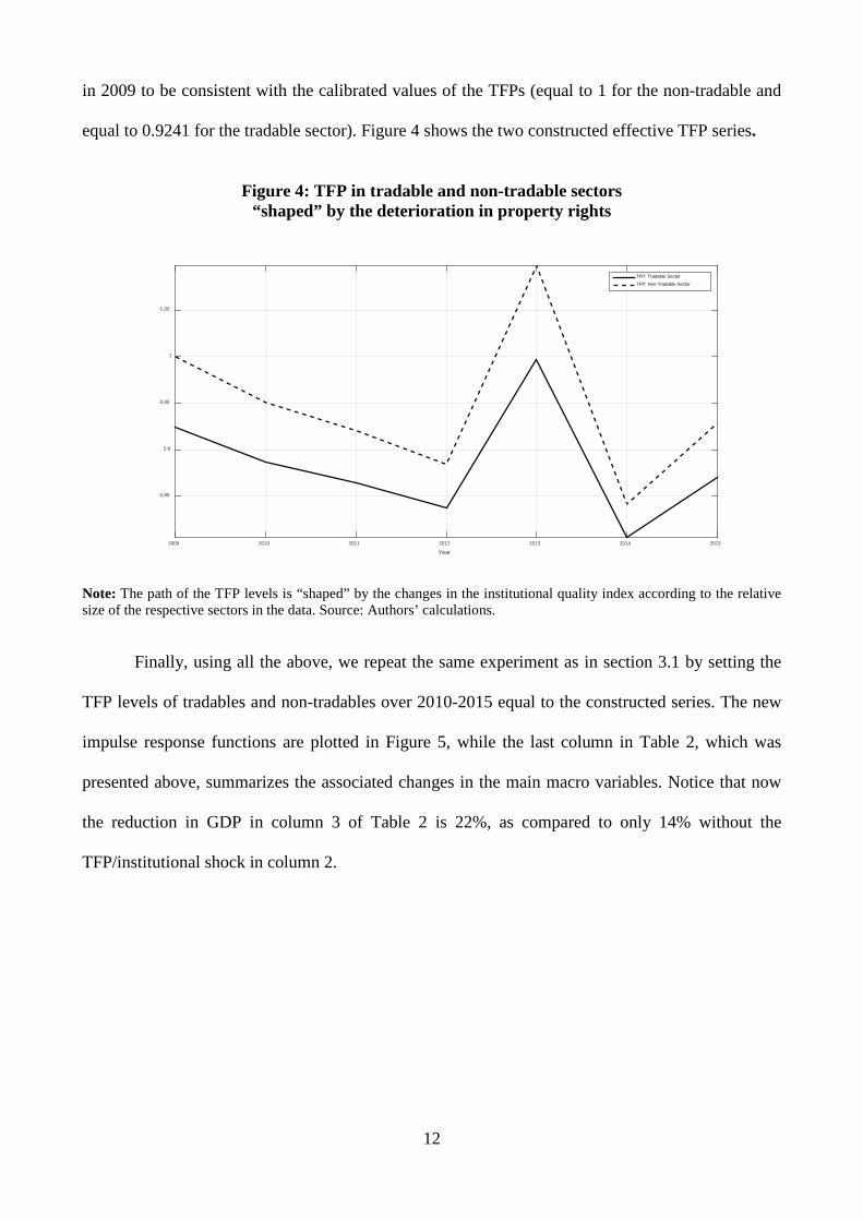
12

in 2009 to be consistent with the calibrated values of the TFPs (equal to 1 for the non-tradable and

equal to 09241 for the tradable sector) Figure 4 shows the two constructed effective TFP series

Figure 4 TFP in tradable and non-tradable sectors

ldquoshapedrdquo by the deterioration in property rights

Note The path of the TFP levels is ldquoshapedrdquo by the changes in the institutional quality index according to the relative size of the respective sectors in the data Source Authorsrsquo calculations

Finally using all the above we repeat the same experiment as in section 31 by setting the

TFP levels of tradables and non-tradables over 2010-2015 equal to the constructed series The new

impulse response functions are plotted in Figure 5 while the last column in Table 2 which was

presented above summarizes the associated changes in the main macro variables Notice that now

the reduction in GDP in column 3 of Table 2 is 22 as compared to only 14 without the

TFPinstitutional shock in column 2

Year2009 2010 2011 2012 2013 2014 2015

085

09

095

1

105

TFP Tradable Sector

TFP Non-Tradable Sector

13

Figure 5 Impulse response functions driven by the fiscal austerity package and the deterioration in property rights

Note All variables are expressed as percentage deviations from the steady-state with the exception of the CPI inflation the interest rate foreign assets and the public debt-to-GDP ratio that are expressed as percentage point deviations

4 Conclusions discussion and extensions

In this paper we studied the quantitative importance of the fiscal austerity program and the

deterioration of institutional quality both as observed in the recent data for the Greek great

depression since 2010 The main result is that the adopted fiscal policy mix and the deterioration in

property rights are the main explanatory variables of the Greek great depression

We close with acknowledging two caveats First here we did not explain why the specific

fiscal policy mix has been chosen (which proves to be particularly distorting) or why the society has

chosen to have weak and deteriorating property rights (which leads to misallocation of resources

and hence to a relatively low TFP) In general it is well recognized that the policies chosen andor

the way resources are (mis)allocated are an equilibrium outcome of a political process interacting

with institutions and distribution (see eg Acemoglu (2009 chapter 4) and Jones (2011)) In the

case of Greece there is no shortage of conjectures about the root causes of such choices which go

back to the post-world war II history of the country Second our analysis here was only positive

One could search for instance for alternative fiscal policy mixes andor institutional regimes that

could perhaps mitigate the recessionary effects of debt consolidation We leave these extensions for

future research

Year2010 2020 2030 2040

D

evia

tion

-30

-20

-10

0Real Output

Year2010 2020 2030 2040

D

evia

tion

-15

-10

-5

0

5Domestic Tradable Output

Year2010 2020 2030 2040

D

evia

tion

-40

-30

-20

-10

0Non-Tradable Output

Year2010 2020 2030 2040

D

evia

tion

-60

-40

-20

0Consumption

TotalRicardianNon-Ricardian

Year2010 2020 2030 2040

D

evia

tion

-60

-40

-20

0

20Private Investment

Year2010 2020 2030 2040

D

evia

tion

-30

-20

-10

0Real Wages-Private Sector

2010 2020 2030 2040

P

oint

Dev

iatio

n

-2

0

2

4CPI Inflation

Year2010 2012 2014 2016 2018

P

oint

Dev

iatio

n

0

1

2

3Interest Rate

Year2010 2020 2030 2040

D

evia

tion

-10

-5

0

5Real Exchange Rate

Year2010 2020 2030 2040

D

evia

tion

-20

-10

0

10Trade Volumes

Exports

Imports

Year2010 2020 2030 2040

P

oint

Dev

iatio

n

-4

-2

0

2Foreign Assets

Year2010 2020 2030 2040

P

oint

Dev

iatio

n

-40

-20

0

20

40Public Debt GDP

14

References

Acemoglu D (2009) Modern Economic Growth Princeton University Press Princeton Anderson D Hunt B amp Snudden S (2014) Fiscal consolidation in the euro area How much pain can structural reforms ease Journal of Policy Modeling 36 785-799 Ardagna S (2001) Fiscal policy composition public debt and economic activity Public Choice 109 301-325 Akitoby B amp Stratmann T (2008) Fiscal policy and financial markets Economic Journal 118 1971-1985 Angelopoulos K Philippopoulos A amp Vassilatos V (2009) The social cost of rent seeking in Europe European Journal of Political Economy 25 280-299 Baldacci E Petrova I Belhocine N Dobrescu G amp Mazraani S (2011) Assessing fiscal stress IMF Working Papers WP11100 Washigton DC Bergoeing R Kehoe P Kehoe T and Soto R (2002) Policy driven productivity in Chile and Mexico in the 1980s and 1990s American Economic Review 92 16-21 Blanchard O amp Gali J (2007) Real wage rigidities and the new Keynesian model Journal of Money Credit and Banking 39 35-65 Cacciatore M Duval R amp Fiori G (2012) Short-term gain or pain A DSGE model based analysis of the short-term effects of structural reforms in labour and product markets OECD Economics Department Working Papers no 948 OECD Paris Calvo GA (1983) Staggered prices in a utility-maximizing framework Journal of Monetary Economics 12 383-398 Canova F (2007) Methods for Applied Macroeconomic Research Princeton University Press Princeton CESifo (2016) EEAG Report on the European Economy Munich Chari VV Kehoe P amp McGrattan E (2007) Business cycle accounting Econometrica 75 781-836 Christoffel K Coenen G amp Warne A (2008) The new area-wide model of the Euro area ndash A micro-founded open-economy model for forecasting and policy analysis European Central Bank Working Paper Series Number 944 Christoffel K amp Linzert T (2010) The role of real wage rigidities and labor market frictions for unemployment and inflation dynamics Journal of Money Credit and Banking 42 1435-1446 Christiano LJ amp Eichenbaum M (1992) Current real business cycle theories and aggregate labor market fluctuations American Economic Review 82 430-450 Christiano LJ Eichenbaum M amp Evans C (2005) Nominal rigidities and the dynamic effects of a shock to monetary policy Journal of Political Economy 113 1-45

15

Christiano LJ Trabandt M amp Walentin K (2011) DSGE models for monetary policy analysis In Friedman BM Woodford M (Eds) Handbook of Macroeconomics Volume 3 Elsevier North-Holland 285ndash367 Coenen G Mohr M amp Straub R (2008) Fiscal consolidation in the euro area long run benefits and short-run costs Economic Modeling 25 912-932 Coenen G Straub R amp Trabandt M (2013) Gauging the effects of fiscal stimulus packages in the euro area Journal of Economic Dynamics and Control 32 367-386 Corsetti G Kuester K Meier A amp Muller G (2013) Sovereign risk fiscal policy and macroeconomic stability Economic Journal 123 F99-F132 Duval R (2008) Is there a role for macroeconomic policy in fostering structural reforms Panel evidence for OECD countries over the past two decades European Journal of Political Economy 24 491-502 Economides G Park H amp Philippopoulos A (2007) Optimal protection of property rights in a general equilibrium model of growth Scandinavian Journal of Economics 109 153-175 Economides G Kalyvitis S amp Philippopoulos A (2008) Does foreign aid distort incentives and hurt growth Theory and evidence from 75 aid-recipient countries Public Choice 134 463-488 Economides G Papageorgiou D Philippopoulos A amp Vassilatos V (2013) Smaller public sectors in the Euro Area Aggregate and distributional implications CESifo Economic Studies 59 536-558 Eggertsson G Ferrero A amp Raffo A (2014) Can Structural reforms help Europe Journal of Monetary Economics 61 2-22 Erceg JC amp Linde J (2013) Fiscal consolidation in a currency union Spending cuts vs tax hikes Journal of Economic Dynamics and Control 37 422-445 European Commission (2010) The economic adjustment programme for Greece European Economy Occasional Papers Number 61 Brussels European Commission (2014) Public Finances in EMU Brussels European Commission (2015) Public Finances in EMU Brussels Forni L Monteforte L amp Sessa L (2009) The general equilibrium effects of fiscal policy estimates for the euro area Journal of Public Economics 93 559-585 Forni L Gerali A amp Pisani M (2010a) The macroeconomics of fiscal consolidations in euro area countries Journal of Economic Dynamics and Control 34 1791-1812 Forni L Gerali A amp Pisani M (2010b) Macroeconomic effects of greater competition in the service sector The case of Italy Macroeconomic Dynamics 14 677-708 Forni L amp Pissani M (2013) Macroeconomic effects of sovereign restructuring in a Monetary Union A model-based approach IMF Working Paper Number 13269

16

Gali J Lopez-Salido D amp Valles J (2007) Understanding the effects of government spending on consumption Journal of the European Economic Association 5 227-270 Garcia-Cicco J Pancrazi R amp Uribe M (2010) Real Business Cycles in Emerging Countries American Economic Review 100 2510-2531 Gerali A Notarpietro A and Pisani M (2014) Macroeconomic effects of simultaneous implementation of reforms after the crisis Bank of Italy Working Paper Number 997 Gerali A Notarpietro A amp Pisani M (2015) Structural reforms investment and zero lower bound in a monetary union Manchester School 83 120-139 Gogos S Mylonidis N Papageorgiou D amp Vassilatos V (2014) 1979-2001 A Greek great depression through the lens of neoclassical growth theory Economic Modelling 36 316-331 Gomes S Jacquinot P Mohr M amp Pisani M (2013) Structural reforms and macroeconomic performance in the euro area countries A model-based assessment International Finance 16 23- 44 Gourinchas P-O Philippon T amp Vayanos D (2016) The analytics of the Greek crisis Mimeo London School of Economics Hall R (2003) Wage determination and employment fluctuations NBER Working Paper Number 9967 Hall R (2005) Employment fluctuations with equilibrium wage stickiness American Economic Review 95 50-64 Heylen F Hoebeeck A amp Buyse T (2013) Government efficiency institutions and the effects of fiscal consolidation on public debt European Journal of Political Economy 31 40-59 IMF (2015a) Euro area policies 2015 Article IV consultation Country Report Number 15204 International Monetary Fund Washington IMF (2015b) Fiscal monitor - Now is the time Fiscal policies for sustainable growth International Monetary Fund Washington Jones C (2008) Macroeconomics Norton and Company New York Jones C (2011) Misallocation economic growth and input-output economics NBER Working Paper Number 16742 Kaufmann D Kraay A amp Mastruzzi M (2010) The worldwide government indicators Methodology and analytical issues World Bank Policy Research Working Papers Number 5430 Kehoe T amp Prescott E (2002) Great depressions of the 20th century Review of Economic Dynamics 5 1-18 Kliem M amp Uhlig H (2013) Bayesian estimation of a DSGE model with asset prices Deutsche Bundesbank Discussion Paper Number 372013

17

Malley J Philippopoulos A amp Woitek U (2009) To react or not Fiscal policy volatility and welfare in the EU-3 European Economic Review 53 689ndash714 Mendoza E (2010) Sudden stops financial crises and leverage American Economic Review 100 1941-1966 Mertens K amp Ravn M (2011) Understanding the aggregate effects of anticipated and unanticipated policy shocks Review of Economic Dynamics 14 27ndash54 OECD (2013) Economic Policy Reforms Going for Growth Paris OECD (2015) Economic Policy Reforms Going for growth Paris Papageorgiou D Efthimiadis T amp Konstantakopoulou I (2012) Effective tax rates in Greece Centre of Planning and Economic Research (KEPE) Discussion Paper Series Number 124 Papageorgiou D (2012) Fiscal policy reforms in general equilibrium the case of Greece Journal of Macroeconomics 34 504-522 Papageorgiou D (2014) BoGGEM A dynamic stochastic general equilibrium model for policy simulations Bank of Greece Working Paper Number 182 Papageorgiou D amp Vourvachaki E (2016) Macroeconomic effects of structural reforms and fiscal consolidations Trade-offs and complementarities European Journal of Political Economy Available from httpdxdoiorg101016jejpoleco201608010 Petrongolo B amp Pissarides C (2001) Looking into the black box A survey of the matching function Journal of Economic Literature 38 390-431 Philippopoulos A Vassilatos V and Varthalitis P (2016) Fiscal consolidation in an open economy with sovereign premia and without monetary policy independence International Journal of Central Banking forthcoming Prescott E (2002) Prosperity and depression American Economic Review 92 1-15 Roeger W amp in lsquot Veld J (2013) Expected sovereign defaults and fiscal consolidations European Economy Economic Papers no 479 Schmitt-Groheacute S amp Uribe M (2003) Closing small open economies Journal of International Economics 61 163-185 Schuknecht L von Hagen J amp Wolswijk G (2009) Government risk premiums in the bond market EMU and Canada European Journal of Political Economy 25 371-384 Stahler N amp Thomas C (2012) Fimod ndash A DSGE model for fiscal policy simulations Economic Modelling 29 239-261 Uhlig H (2007) Explaining asset prices with external habits and wage rigidities in a DSGE model American Economic Review 97 239-243 Vogel L (2012) Structural reforms fiscal consolidation and external rebalancing in monetary union A model-based analysis Economic Modelling 29 1286-1298

18

Vogel L (2014a) Nontradable sector reform and external rebalancing in monetary union A model-based analysis Economic Modelling 29 1286-1298 Vogel L (2014b) Structural reforms at the zero bound European Economy Economic Papers no 537

19

1 Namely the drop in output is large occurred rapidly and is sustained this is defined as a ldquogreat depressionrdquo See Gogos et al (2014) for an application of this methodology to the Greek economy before the euro period 2 There is a growing literature on the current Greek crisis For instance Bortz (2015) discusses where the financial assistance has gone offering a different view from that of Sinn (2015) Arellano and Bai (2016) study the Greek default Papageorgiou and Vourvachaki (2016) study the implications of structural reforms in light of the crisis Gourinchas et al (2016) search for shocks that can account for the Greek crisis See below for further details 3 See eg Philippopoulos et al (2016) for the different implications of different fiscal policy mixes used for debt consolidation in Italy 4 Alternatively we could for instance use a VAR approach which requires a limited amount of theory to structure the data (see eg Canova 2007 for methodology) We prefer to follow the DSGE approach so as to have well-defined micro-foundations that allow us to understand the behavioral channels through which exogenous changes affect macroeconomic outcomes 5 There is a large literature that shows how weak institutions affect the efficiency with which factor inputs are used and in particular how weak property rights lead to distortive individual incentives resource misallocation and eventually a lower level of total factor productivity See eg Jones (2008 chapter 4 and 2011) and Acemoglu (2009 chapter 4) for reviews of the literature while see below for further details and references Here working as in Chari et al (2007) we will take a short cut by assuming that changes in property rights directly show up as shocks to TFP nevertheless as argued in subsection 32 below this is equivalent to a richer model where the adverse effect of weak property rights on TFP works via the distortion of individual incentives 6 See eg Chari et al (2007) for a methodology paper on business cycle accounting 7 We focus on the period during which Greece is part of the euro area but before the debt crisis erupted in early 2010 8 In particular we assume that ( ) 1G H

t t tR mR m R= + minus where we set the value of m equal to 05

9 In the same spirit Economides et al (2007 2008) and Angelopoulos et al (2009 2012) also provide micro-founded dynamic general equilibrium models where the presence of weak property rights distorts private incentives and in equilibrium this leads to resource misallocation which in turn maps into reductions in the effective TFP All this belongs to a rich and still growing literature that endogenizes the TFP and hence endogenizes long-term growth 10 The rule of law indicator captures perceptions of the extent to which agents have confidence in and abide by the rules of society and in particular the quality of contract enforcement property rights the police and the courts as well as the likelihood of crime and violence The regulatory quality index captures perceptions of the ability of the government to formulate and implement sound policies and regulations and the credibility of governmentrsquos commitment to such policies The political stability and absence of violenceterrorism indicator captures perceptions of the likelihood that the government will be destabilized or overthrown by unconstitutional or violence means including politically-motivate violence and terrorism For further details see Kaufman et al (2010) We report that each one of these three sub-indexes is highly correlated with key macroeconomic variables such as real GDP and real investment in the Greek data

20

Appendix A A DSGE model and calibration

This appendix presents the model used It is similar to that in Papageorgiou (2014)

1 Households

The economy is populated by a continuum of households of mass one indexed by [ ]01hisin of

which a fraction indexed by [01 ]i λisin minus are referred as ldquoRicardianrdquo or ldquooptimizing householdsrdquo

and a fraction indexed by (1 1]j λisin minus are referred as ldquonon-Ricardianrdquo or ldquoliquidity constrained

householdsrdquo Optimizing households have access to capital and financial markets where they can

invest in the form of physical capital government bonds and internationally traded assets Liquidity

constrained households on the other hand are not able to lend or borrow so that they consume

their disposable labor income in each time period Both households supply differentiated labor

services and act as wage-setters in monopolistically competitive markets

11 Ricardian households

Ricardian households indexed by i have preferences over consumption and leisure The inter-

temporal utility function of each i is

( )10 0

Rt cti i t i t

tU E u C C Hβ ξ

infin

minus

=

= minussum (1)

where (01)β isin is the discount factor i tC is i rsquos effective consumption (defined below) at t i tH is

i rsquos total work hours at t [01)cξ isin is a parameter that measures the degree of external habit

formation in consumption and 1RtC minus denotes average (per household i ) lagged-once effective

consumption Effective consumption is in turn defined to be a linear combination of private

consumption p

i tC and public goods and services (education health etc) provided by the state

sector gtY 1

p g

i t i t tC C Yϑ= + (2)

where [ 11]ϑisin minus is the degree of substitutability between private and public consumption

The instantaneous utility function is assumed to be of the form

( ) ( )1

1 1 log

1

R R i tc ct ti t i t i t

Hu C C H C C

g

ξ ξ κg

+

minus minusminus = minus minus+

(3)

1 See eg Christiano and Eichenbaum (1992) Forni et al (2010a) and Economides et al (2013)

21

where g is the inverse of Frisch labour supply elasticity and 0κ gt is a preference parameter

related to work effort Each household i supplies work hours in the private sector p

i tH and the

public sector gi tH As in eg Ardagna (2001) and Forni et al (2009) hours of work can be moved

across the two sectors and are perfect substitutes in terms of (dis)utility so that p g

i t i t i tH H H= + in

each period t

The Ricardian household can save in the form of physical capital p

i tI domestic government

bonds i tB and foreign assets p

i tF It receives labour income from working in the private sector

p p

i t i tw H and the public sector g gi t i tw H where

pi tw and

gi tw are the real wage rates in the private and

public sector respectively The household rents out capital to firms and receives capital income

k p

t i t i tr u K where ktr is the real return to the effective amount of private capital

pi tK is the physical

private capital stock and 0i tu gt is the utilization rate of capital The household also earns interest

income from domestic government bonds and internationally traded assets that pay a gross nominal

interest 1tR ge and 1HtR ge at 1t + respectively In addition households own all domestic firms so

that they receive their profits as dividends i tDiv Finally each Ricardian household receives a

lump-sum government transfer tri tG The household pays taxes on consumption 0 1c

ttlt lt on

labour income 0 1lttlt lt on capital earnings and dividends 0 1k

ttlt lt and lump-sum taxes tT

Hence the budget constraint of each Ricardian household i is

( )

( )( ) ( )( )

1 1

1

1

1 1

pIi t t i tc p pt

t i t i tC C Ct t t

l p p g g k k pt i t i t i t i t t t i t i t i t

t

B S FPC IP P P

w H w H r u K Div

R

t

t t

+ +

minus

+ + + + =

= minus + + minus + +

+ 1

pi t t i tH tr h

t i t t i tC Ct t

B S FR G T

P Pminus+ + minus minusG

(4)

where CtP and I

tP are the prices of a unit of the private consumption final good and the investment

final good respectively and tS is the nominal exchange rate (expressed in terms of domestic

currency per unit of foreign currency) The household faces costs when it adjusts its private foreign

asset holdings hi tG whenever the private foreign assets-to-GDP ratio GDP

tY

t

ptit

YPFS 1 + deviates from its

long-run target level f In particular

( )2

1 1

2

pY GDPft i th p Y GDP C t t

i t t i t t t t C Y GDPt t t

S FP YS F P Y P fP P Y

ξ ++

G = minus

(5)

22

where GDPtY is the economyrsquos real GDP Y

tP is the GDP deflator and 0gefξ is an adjustment cost

parameter2

The private capital stock evolves over time according to the following law of motion

( )( ) 1

1

1 1p

i tp p p I pi t i t i t i tp

i t

IK u K I

Iδ+

minus

= minus + minusΨ

(6)

where IΨ is a convex adjustment cost function for investment as in eg Christiano et al (2005)

2

1 1

12

p pki t i tIp p

i t i t

I II I

ξ

minus minus

Ψ = minus

(7)

where (1) (1) 0I IΨ = Ψ = and 0kξ ge is an adjustment cost parameter We assume that the

depreciation rate of private capital depends on the rate of capacity utilization and is a convex

function that satisfies 0pδ prime gt 0pδ primeprime gt so that ( ) p p

i t i tu uϕδ δ= where (01)pδ isin and 0ϕ gt are

respectively the average rate of depreciation of private capital and the elasticity of marginal

depreciation cost

The first-order conditions of this problem are written below when we present the final

equilibrium system

12 Non-Ricardian households

Liquidity constrained households indexed by j have the same preferences as Ricardian

households They receive labour income from working in the private and public sectors but have no

access to capital or financial markets so that in each period their consumption spending equals

their after-tax wage income plus lump-sum government transfers The period-by-period budget

constraint of each household j is

( ) ( )( ) 1 1c l p p g g trt j t t j t j t j t j t j tC w H w H Gt t+ = minus + + (8)

where pj tH and

gj tH are respectively hours worked in the private and public sector by household j

and trj tG is a lump-sum government transfer to each j Thus as in eg Coenen et al (2013) we

allow for a potentially uneven distribution of government transfers across Ricardian and non-

Ricardian households

The first-order conditions of this problem are written below when we present the final

equilibrium system

2 This specification ensures that foreign private assets are stationary see eg Schmitt-Grohe and Uribe (2003)

23

2 Wage setting and the evolution of wages in the private sector

We assume that wages in the private sector are set by monopolistic unions as in eg Forni et al

(2009) and Gali et al (2007) More specifically households supply differentiated labour varieties to

a continuum of unions [ ]01hisin each of which represents a specific labour variety Every variety is

uniformly distributed across households so that each union ultimately represents 1 λminus fraction of

Ricardian households and λ of non-Ricardian households In every period each union sets the

wage rate for its own workers by trading off the utility derived from private sector labour income

and the disutility of total work effort by taking into account the demand for the differentiated labour

variety h At the same time private and public sector firms allocate their labour demand uniformly

across the h labour varieties independently of the type of households which implies that hours

worked by each type of household are equal

h p h p pj t i t h tH H H= equiv and

h g h g gj t i t h tH H H= equiv 3

Therefore in each period a typical union h chooses the wage rate ph tw to maximize

( ) ( ) ( )1

1 1 1

1h tNR l p p R l p p

w h t h t h t h t h t h t

HL w H w H

g

λ t λ t κg

+

= L minus + minus L minus minus + (9a)

subject to

1

Wt

Wt

ph tp p

h t tpt

wH H

w

micromicro

minusminus

=

(9b)

p g

h t h t h tH H H= + (9c)

where Eq (9b) is the demand for the differentiated labour input h ptH is total labour demand in the

private sector ptw is the aggregate wage rate in the private sector and

NRh tL

Rh tL are the marginal

utilities of consumption of non-Ricardian and Ricardian households of labour variety h

respectively used as weights Finally ( ) 1 1W Wt tmicro micro minus gt is the elasticity of substitution across the

differentiated labour services where 1Wtmicro gt is the wage markup in the private labour market

Focusing on a symmetric equilibrium in which all unions choose the same wage rate ex

post the first-order condition of the above problem is

1p Wt tNR R

t t

wMRS MRS

λ λ micro minus

+ =

(10)

3 Total public sector labour demand for the differentiated labour input ℎ is exogenous and is defined as 1

0

g gt h tH H dh= int

24

where ptw is the optimal wage rate chosen by unions and NR

tMRS and RtMRS are the marginal

rates of substitution between consumption and leisure of non-Ricardian and Ricardian households

respectively4

Following eg Hall (2005) and Blanchard and Gali (2007) we introduce further rigidities in

the labour market by assuming that real wages respond sluggishly to labour market conditions In

particular the real wage rate in the private sector is modeled as a weighted average of the lagged-

once real wage rate and the optimal real wage rate chosen by unions

( ) ( )11

n np p pt t tw w w

minus

minus= (11)

where 0 1nle le denotes the degree of real wage rigidities and ptw is given by (10)5 This

formulation aims to capture the rigidities found in the Greek labour market (see eg the discussion

in European Commission 2010)6

3 Production in the private sector

There are two types of domestic firms The first type consists of monopolistically competitive firms

that produce intermediate goods tradable and non-tradable The continuum of firms producing

differentiated varieties of tradables indexed by [ ]01Tf isin sell their output domestically or abroad

(the latter are recorded as exports) The continuum of firms producing differentiated varieties of

non-tradables indexed by [ ]01Nf isin sell their output domestically only There is also a continuum

of monopolistically competitive firms importing intermediate goods indexed by [ ]01Mf isin The

second type of firms consists of four perfectly competitive firms that produce final goods These

firms combine purchases of intermediate goods to produce four non-tradable goods a private

consumption good a private investment good a public consumption good and a public investment

good Finally there is a foreign final goods firm that combines purchases of the exported domestic

intermediate goods

4 Note that when 0λ = ie when all households are Ricardian W

tmicro reduces to a markup of the optimally chosen real

wage rate over the marginal rate of substitution between consumption and leisure of Ricardian households 5 See also eg Uhlig (2007) Malley et al (2009) and Kliem and Uhlig (2013) for a similar specification Microfoundations for Eq (11) can be found in eg Hall (2003) Petrongolo and Pissarides (2001) and Christoffel and Linzert (2010) 6 Papageorgiou (2014) finds that this specification can capture rather well the aggregate dynamics of work hours and real wages in Greece

25

31 Final goods firms

As said above there are four representative final goods firms that combine purchases of tradable

intermediate goods with non-tradable goods to produce a private consumption good ptC a private

investment good ItI a public consumption good gc

tG and a public investment good gitG

Private consumption goods producer

The representative producer of the private final consumption good combines a bundle of tradable

consumption intermediate goods TtC with a bundle of non-tradable intermediate goods N

tC

according to a constant elasticity of substitution (CES) production function

( ) ( )1 11 1 1

(1 )

C

C C CC CC C

p T Nt C t C tC C C

εε ε ε

ε εε εω ωminus minus minus

= + minus

(12)

where [ ]01Cω isin measures the weight of tradable goods in the production of the final private

consumption good and 0Cε gt is the elasticity of substitution between tradable and non-tradable

consumption goods

In turn the tradable intermediate consumption good bundle is a CES function of the

domestically produced bundle of tradable intermediate consumption goods DtC and the bundle of

imported intermediate consumption goods MtC

( ) ( )1 11 1 1

(1 )

TC

TC TC TCTC TCTC TC

T D Mt TC t TC tC C C

εε ε ε

ε εε εω ωminus minus minus

= + minus

(13)

where [ ]10isinTCω measures the home bias in the production of the tradable intermediate

consumption good and 0TCε gt is the elasticity of substitution between domestic and imported

intermediate consumption goods

The intermediate consumption good bundles that are used as inputs combine differentiated

varieties supplied by intermediate good firms Specifically the varieties supplied by each tradable

intermediate goods firm Tf T

Df t

C each non-tradable intermediate-goods firm Nf N

Nf t

C and each

importing firm Mf M

Mf t

C are respectively combined using a CES technology into

( )1

1

0

Tt

Tt

TD D Tt f t

C C dfmicro

micro

= int (14a)

26

( )1

1

0

Nt

Nt

NN N Nt f t

C C dfmicro

micro

= int (14b)

( )1

1

0

Mt

Mt

MM M Mt f t

C C dfmicro

micro

= int (14c)

where 1T N Mt t tmicro micro micro gt are the intra-temporal elasticities of substitution between different varieties

within each type of intermediate consumption good As we show below T N Mt t tmicro micro micro represent

markups in the markets of domestic and imported intermediate goods

Given the above technology the producer of the final private consumption good solves a

three stage problem In the first stage it takes as given the prices of domestic tradable N

Df t

P non-

tradable T

Nf t

P and imported intermediate goods M

Mf t

P and chooses the amounts of the

differentiated goods T

Df t

C N

Nf t

C M

Mf t

C in order to minimize total expenditures for the bundles of

the differentiated goods 1

0

T TD D Tf t f t

P C dfint 1

0

N NN N Nf t f t

P C dfint 1

0

M MM M Mf t f t

P C dfint subject to the aggregation

constraints in (14a)-(14c) The solution of the cost minimization problem gives the demand

functions for these intermediate goods Tf Nf and Mf respectively

1

Dt

DtT

T

Df tD D

tDf tt

PC C

P

micromicro

minusminus

=

(15a)

1

Nt

NtN

N

Nf tN N

tNf tt

PC C

P

micromicro

minusminus

=

(15b)

1

Mt

MtM

T

Mf tM M

tMf tt

PC C

P

micromicro

minusminus

=

(15c)

where D N Mt t tP P P are the aggregate price indices of domestic tradable non-tradable and imported

intermediate consumption goods respectively

In the second stage the firm chooses the bundles DtC and M

tC in order to maximize its

profits 1C TC T D D M Mt t t t t t tP C P C P CP = minus minus subject to the technology constraint (13) and by taking as

given the price indexes of domestic tradables TCtP non-tradables D

tP and imported intermediate

consumption goods MtP Thus it solves

27

max

D Mt t

TC T D D M Mt t t t t t

C CP C P C P Cminus minus

subject to

( ) ( )1 11 1 1

(1 )

TC

TC TC TCTC TCTC TC

T D Mt TC t TC tC C C

εε ε ε

ε εε εω ωminus minus minus

= + minus

In the third stage the firm chooses the demand for TtC and N

tC to maximize profits

2C C C TC T N Nt t t t t t tP C P C P CP = minus minus subject to the technology constraint (12) and by taking the input

prices CtP TC

tP and NtP as given Thus it solves

max

T Nt t

C C TC T N Nt t t t t t

C CP C P C P Cminus minus

subject to

( ) ( )1 11 1 1

(1 )

C

C C CC CC C

p T Nt C t C tC C C

εε ε ε

ε εε εω ωminus minus minus

= + minus

The demand functions for domestic tradable and imported consumption goods as well as for

tradable and non-tradable intermediate consumption goods resulting from the optimization problem

of the final consumption good firm are

TCD Dt t

TCT TCt t

C PC P

ε

ωminus

=

(16a)

( )1TCM M

t tTCT TC

t t

C PC P

ε

ωminus

= minus

(16b)

CT TCt t

CC Ct t

C PC P

ε

ωminus

=

(16c)

( )1CN N

t tCC C

t t

C PC P

ε

ωminus

= minus

(16d)

From the zero profit condition we get the price index for tradable consumption goods

( ) ( )( )1

1 1 11TC TC TCTC D M

t TC t TC tP P Pε ε εω ω

minus minus minus = + minus and the price index of a unit of the final consumption

good (ie the Consumption Price Index) ( ) ( ) ( )1

1 1 11C C CC TC N

t C t C tP P Pε ε εω ω

minus minus minus = + minus where

D N Mt t tP P P are the prices of domestic tradable intermediates non-tradable intermediates and

imported intermediate goods respectively

28

Private investment goods producer

Optimal decisions regarding the production of the final private investment good are derived in an

analogous manner as above The representative producer of the private investment good combines a

composite bundle of tradable intermediate goods TtI with a bundle of non-tradable intermediate

goods NtI to generate a composite final private investment good I

tI by using a constant elasticity

of substitution (CES) production function

( ) ( )1 11 1 1

(1 )

I

I I II II I

I T Nt I t I tI I I

εε ε ε

ε εε εω ωminus minus minus

= + minus

where [ ]01Iω isin measures the weight of tradable goods in the production of the final private

investment good and 0Iε gt is the elasticity of substitution between tradable and non-tradable

investment goods

In turn the composite bundle of the tradable intermediate investment good that is used in the

production of final investment goods is a CES function of domestically produced tradable

intermediate investment goods DtI and imported intermediate investment goods M

tI

( ) ( )1 1 11 1

(1 )

TI

TITI TITI TITI TI

T D Mt TI t TI tI I I

εεε ε

ε εε εω ωminusminus minus

= + minus

where [ ]01TIω isin measures the home bias in the production of the tradable intermediate

consumption good and 0TIε gt is the elasticity of substitution between domestic and imported

investment goods

The demand functions for domestic tradable and imported investment goods as well as for

tradable and non-tradable investment goods are

TID Dt t

TIT TIt t

I PI P

ε

ωminus

=

( )1TIM M

t tTIT TI

t t

I PI P

ε

ωminus

= minus

IT TIt t

II It t

I PI P

ε

ωminus

=

( )1IN N

t tIT I

t t

I PI P

ε

ωminus

= minus

29

where ( ) ( )( )1

1 1 11TI TI TITI D M

t TI t TI tP P Pε ε εω ω

minus minus minus = + minus and ( ) ( )( )

11 1 11

I I II TI Nt I t I tP P P

ε ε εω ωminus minus minus = + minus

are respectively the price indices for tradable intermediate investment goods and final investment

goods

Public consumption and investment goods production

Regarding the final public consumption and investment goods gctG and gi

tG we assume they are

produced using only non-tradable intermediate goods Hence gc Nt tG GC= and gi N

t tG GI= where

( )1

1

0

Nt

Nt

NN N Nt f t

GC GC dfmicro

micro

= int and ( )

11

0

Nt

Nt

NN N Nt f t

GI GI dfmicro

micro

= int

The optimal demand functions are

1

Nt

NtN

N

Nf tN N

tNf tt

PGC GC

P

micromicro

minusminus

=

and 1

Nt

NtN

N

Nf tN N

tNf tt

PGI GI

P

micromicro

minusminus

=

Aggregating across final good producing firms we get the respective aggregate domestic demand

functions for non-tradable domestic tradable and imported intermediate goods Tf Nf and mf

1

Nt

NtN

N N N N N

Nf tNT N N N N NT

tNf t f t f t f t f tt

PY C I GC GI Y

P

micromicro

minusminus

= + + + =

1

Tt

TtT

T T T

Df tD D D D

tDf t f t f tt

PY C I Y

P

micromicro

minusminus

= + =

1

Mt

MtM

M M M

mf tM M M M

tmf t f t f tt

PY C I Y

P

micromicro

minusminus

= + =

where NT N N N Nt t t t tY C I GC GI= + + + D D D

t t tY C I= + and M M Mt t tY C I= + are respectively the total

demand for non-tradable goods total domestic demand for domestically produced tradable goods

and total demand for imports

32 Intermediate goods firms

Each tradable and non-tradable intermediate good Tf t

Y and Nf t

Y is produced by a continuum of

monopolistically competitive intermediate goods firms indexed by [ ]01Tf isin and [ ]01Nf isin

respectively according to the production technologies

30

( ) ( ) ( )1

T T G

T T T

a a aT gt t Tf t f t f t

Y A K H Kminus

= minusΦ (17a)

( ) ( ) ( )1

N N G

N N N

a a aN gt t Nf t f t f t

Y A K H Kminus

= minusΦ (17b)

where Tf t

K is private capital Tf t

H is work hours in the private sector gtK is public capital

0T Na a gt are the output elasticities of capital services in the tradable and non-tradable sectors

respectively and 0Ga gt is the output elasticity of public capital7 Finally 0T NΦ Φ ge are fixed

costs of production and TtA N

tA are sector-specific total factor productivity levels

Tradable sector

In what follows we present the problem of intermediate goods firms in the tradable sector

Domestic intermediate goods firms in the tradable sector solve a two-stage problem In the first

stage each firm takes as given factor prices ktr and p

tw and chooses capital and labour inputs

Tf tK and

Tf tH in order to minimize total real input cost We also introduce a working capital

channel in the form of a ldquocash-in-advancerdquo constraint in the spirit of eg Mendoza (2010) In

particular at the beginning of each period each firm borrows from international lenders in order to

cover a fraction (01)tv isin of their total labour costs in advance of revenuesrsquo receipt The working

capital loan is repaid by the end of the period at the domestic country gross interest rate HtR Thus

the intratemporal problem of each firm involves the minimization of their costs inclusive of the

costs of serving their intra-period working capital loan In other words

( )

min 1T T TT Tf t f t

k p H pt t t t tf t f t f tK H

r K w H R v w H+ + minus (18)

subject to (17a)

The first-order conditions are

( )( ) ( )

1 1 1T

T

T

Tf tH pt t t T f t

f t

YR w a mc

Hν

+Φ+ minus = minus (19)

T

T

T

Tf tkt T f t

f t

Yr a mc

H

+Φ= (20)

where Tf t

mc is the Lagrange multiplier associated with the technology constraint that is the real

marginal cost in terms of the consumer prices CtP Because firms borrow to cover part of their

7 These production functions have increasing returns to scale with respect to all inputs and constant returns to scale with respect to private inputs (see also eg Baxter and King (1993) and Leeper et al (2010))

31

labour costs the marginal cost of labour is higher than the wage rate in the private sector As a

result increases in either the share of labour costs that are financed through working capital loans

or in the domestic interest rate directly increase the cost of labour and thereby reduce labour

demand

The labour input Tf t

H is a composite aggregate of household-specific varieties T

hf t

H

( )1

1

0

Wt

Wt

T Th

f t f tH H

micro

micro

= int Optimal demand is

1

Wt

T T

ph thpf t f t

t

wH H

w

micro =

where ( 1) 1W Wt tmicro micro minus gt is the

elasticity of substitution across differentiated labour services and ptw is the aggregate real wage

index in the private sector that is given by ( )11

1 10

Wt

Wtp p

t h tw wmicro

micro

minus

minus

= int

In the second stage intermediate good firms in the tradable sector choose the price that

maximizes discounted real profits As in Christoffel et al (2008) firms charge different prices at

home and abroad setting prices in producer currency In both domestic and foreign markets we

assume that prices are sticky aacute la Calvo (1983) In particular each period t the firm Tf optimally

resets prices with a constant probability 1 Dpθminus when it sells its differentiated product in the

domestic market and with probability 1 Xpθminus when it sells its product abroad The firms that cannot

optimize partially index their prices to aggregate past inflation according to the price indexation

schemes ( )1 1

D

T T

xD D Dtf t f t

P P minusminus= P and ( )1 1

X

T T

xX X Xtf t f t

P P minusminus= P where

TDf t

P denote the domestic price of

good Tf T

Xf t

P its foreign price and 1D D Dt t tP PminusP = 1X X X

t t tP PminusP = where D Xt tP P are the

aggregate domestic and export price indices (defined below) respectively The indexation

parameters [ ] 01D Xx x isin determine the weights given to past inflation

Each firm Tf which can optimally reset its price in period t knows with probability Dpθ

that this price will continue to be in effect t periods ahead and so chooses the optimal price

TD

f tP

to maximize the discounted sum of expected real profits (in terms of consumer prices CtP ) by

taking aggregate domestic demand DtY and the aggregate price index in the domestic market D

tP

as given Thus each firm Tf maximizes

( ) ( )

1

0 1

maxTD

TDTf t

DR Dx f tD D D Dt tt p t s tR D Df tP st t t

P PE mc YP P

t tt t

t tt t t

βθinfin

+ ++ minus + +

= = + +

L P minus L sum prod (21)

32

subject to

( )1

1

1

Tt

TtTD

T

Dx f tD D D

t s tDf ts t

PY Y

P

t

t

micromicrot

tt

+

+

minusminus

+ minus += +

= P prod (22)

where D C T Dt t t tmc P mc P= is the real marginal cost in terms of the domestic price index and

R Rt tt+L L is the ratio of the marginal utilities of consumption of Ricardian households - that are the

owners of the firms - according to which firms value future profits8 Notice that since all firms face

the same marginal cost and take aggregate variables as given any firm that optimizes will set the

same price

TD D

tf tP P=

Thus the first-order condition of the above problem is

( ) ( ) ( )1

1 1

1 1

0

Tt

TD Dtx xD DR D D D

t s t sD D T Dt t t tt p t t tR D D D D D

s st t s t t t s t

P P PE Y mcP P P

t

t

micromicro

t tt t tt t t

t

βθ micro

+

+

minusminus

+ minus + minus+ ++ + +

= =+ + +

P PL minus = L P P

prod prod (23)

According to the above expression firms set nominal prices so as to equate the average future

expected marginal revenues to average future expected marginal costs9 The aggregate domestic

index evolves according to ( )( ) ( )( )111

1 11 11

Tt

TDT ttxD D D D D D

t p t p t tP P Pmicro

micromicroθ θ

minus

minusminusminus minus

= minus + P

Similarly the associated first-order condition of each firm Tf that chooses its price in the

foreign market in period t is

( ) ( ) ( )1

1 1

1 1

0

Xt

XX Xtx xX XR X X X

t s t sX X X Xt t t tt p t t tR X X C X X

s st t s t t t s t

P P PE Y mcP P P

t

t

micromicro

t tt t tt t t

t

βθ micro

+

+

minusminus

+ minus + minus+ ++ + +

= =+ + +

P PL minus = L P P

prod prod (24)

where X C T Xt t t tmc P mc P= is the real marginal cost in terms of the aggregate export price index and

the aggregate export price index is ( )( ) ( )( )111

1 11 11

Xt

XXx ttxX X X X X X

t p t p t tP P Pmicro

micromicroθ θ

minus

minusminusminus minus

= minus + P

8 In equilibrium the marginal utility of consumption is common across Ricardian households

Ri t tL = L

9 In the case of fully flexible prices 0Dpθ = the above condition reduces to the static relation D T C T

t t t tP P mct tmicro + +=

which states that the price is equal to a markup over the nominal marginal cost

33

Non-tradable sector

The optimal demand by each firm Nf for labour of type h is

1

Wt

Wt

N N

ph thpf t f t

t

wH H

w

micromicro

minusminus

=

and the

aggregate demand for labour of type h is

11

0

Wt

Wt

N

ph tN h N

h t tpf tt

wH H df H

w

micromicro

minusminus

= =

int where NtH is total

labour demand in the non-tradable intermediate good sector As in the case of the tradable good

firms non-tradable intermediate good firms take short-term loans from international lenders at the

home countryrsquos gross interest rate HtR in order to finance a fraction tv of their total labour costs

To minimize costs each firm takes as given the factor prices ktr and p

tw and chooses N Nf t f t

K H

in order to minimize total real input cost ( ) 1N N N

k p H pt t t t tf t f t f t

r K w H R v w H+ + minus subject to the

production function The first-order conditions are

( )( ) ( )

1 1 1N

N

N

Nf tH pt t t N f t

f t

Yv R w a mc

H

+Φ+ minus = minus

N

N

N

Tf tkt N f t

f t

Yr a mc

K+Φ

=

where due to symmetry N

Ntf t

mc mc=

Non-tradable intermediate good firms face price stickiness aacute la Calvo with 1 Npθminus being the

probability that a firm Nf can optimally reset its price in any given period 0t ge The optimal

pricing is characterized by the following conditions

( ) ( ) ( )1

1 1

1 1

0

Nt

Nd Ntx xN NR N N N

t s t sN N N Nt t t tt p t t tR N N C N N

s st t s t t t s t

P P PE Y mcP P P

t

t

micromicro

t tt t tt t t

t

βθ micro

+

+

minusminus

+ minus + minus+ ++ + +

= =+ + +

P PL minus = L P P

prod prod

and the aggregate domestic index evolves according to

( )( ) ( )( )111

1 11 11

Nt

NNN ttxN N N N N N

t p t p t tP P Pmicro

micromicroθ θ

minus

minusminusminus minus

= minus + P

Importing firms

There is a continuum of importing firms [ ]01Mf isin each of which imports a single differentiated

intermediate good M

Mf t

Y These firms operate under monopolistic competition so that they have

34

pricing power This creates a wedge between the price at which the importing firms buy the foreign

differentiated goods in the world markets Yt tS P and the price at which they sell these goods to

domestic households M

Mf t

P Importing firms face price stickiness aacute la Calvo with 1 Mpθminus being the

probability that a firm Mf can optimally reset its price in the domestic market in any given period

0t ge so that optimal pricing follows

( ) ( ) ( )1

1 1

1 1

0

Mt

Mm mtx xM MR M M M

t s t sm M M Mt t t tt p t t tR M M C M M

s st t s t t t s t

P P PE Y mcP P P

t

t

micromicro

t tt t tt t t

t

βθ micro

+

+

minusminus

+ minus + minus+ ++ + +

= =+ + +

P PL minus = L P P

prod prod

and the aggregate import price index evolves according to

( )( ) ( )( )111

1 11 11

Mt

MmM ttxM m M m M M

t p t p t tP P Pmicro

micromicroθ θ

minus

minusminusminus minus

= minus + P

33 Demand from foreign final goods firms

We now model the demand coming from foreign firms or equivalently specify the domestic

countryrsquos exports Recall that the domestic economy produces intermediate tradable goods that are

also exported and so we need to model a final goods firm that transforms them into final goods

There is a representative foreign final good firm that purchases the differentiated exported goods

X

f tY produced by the domestic tradable intermediate good firms Tf and transforms them into a

homogeneous final good XtY via the CES technology

( )1

11

0

XtX

tT

X X Tt f t

Y Y dfmicro

micro

= int (25)

where 1Xtmicro gt is related to the intratemporal elasticity of substitution between the differentiated

outputs supplied by domestic intermediate good firms ( ) 1 1X Xt tmicro micro minus gt

The foreign firm takes the prices of exported differentiated goods

TX

tf tP S (expressed in

terms of the foreign currency) as given and chooses the optimal amounts of differentiated inputs to

minimize total input costs ( )1

0T T

X X Ttf t f t

P S Y dfint subject to (25) so that the optimal demand function

for each input T

Xf t

Y is 1

Xt

XtT

T

Xf tX X

tXf tt

PY Y

P

micromicro

minusminus

=

where ( )11

11

0

Xt

Xt

TX X T

t f tP P df

micro

micro

minus

minus

= int is the aggregate

price index of exported domestic intermediate goods and XtY is total foreign demand for domestic

35

intermediate goods The latter is

XX

X t tt tX

t

P SY YP

εminus

=

where X

tP is the price of foreign

competitors in the export markets tY is foreign economy output and 0Xε gt is the price elasticity

of export demand

4 The public sector

We now model the public sector

41 Government budget constraint and fiscal policy instruments

The government levies taxes on consumption labour income capital earnings and dividends We

also assume lump-sum taxestransfers The government also sells one-period government bonds to

the domestic bond market 1gtB + and the international market 1

gtF + Total tax revenues plus the issue

of new government bonds are used to finance government consumption ctG investment i

tG

transfers trtG and the wage bill of public sector employees g g

t tw H Moreover the interest rates

that the government pays on inherited domestic public debt and on foreign public debt are tR and

GtR respectively We assume that G

tR is a weighted average of the market interest rate that the

country faces when it borrows from abroad and the risk-free world interest rate (see below for

details) Thus the within-period government budget constraint in per-capita terms is

( ) ( )1 1

1 1

g gc p l p p g g k k pt t tt t t t t t t t t t t t tc C

t tN N g g

c i tr g g Gt t t t tt t t t t t tC C C C

t t t t

B S F C w H w H r u K Div TP P

P P B S FG G G w H R RP P P P

t t t+ +

minus minus

+ + + + + + + =

= + + + + +

(26)

Therefore the government has eleven policy instruments 1 1 c l k g g c i tr g gt t t t t t t t t t t tX T w H G G G B Ft t t + +isin

out of which ten can be exogenously set

To ensure dynamic stability we need to assume that one of the exogenously set fiscal policy

instruments follows a state-contingent rule reacting systematically to deviations of the public debt-

to-GDP ratio from a target level and the rate of change of debt

( ) ( )1 1 2 1d y d y y

t t t t tX X D d D Dφ φminus minus= + minus + minus (27)

where 1 1

y tt y GDP

t t

DDP Yminus minus

equiv denotes the debt-to-GDP ratio in the beginning of period t d is a target value

of the public debt-to-GDP ratio (see below for details) and 1 2 0d dφ φ gt are feedback policy reaction

coefficients (as in a Taylor rule for the nominal interest rate)

36

For notational convenience we will define the share of total public debt held by domestic

agents at the end of period t as 1

1

gt

tt

BD

ζ +

+

equiv where 0 1tζle le so that 1 1(1 )gt t t tS F Dζ+ += minus and

1 1 1g g

t t t tD B S F+ + += +

42 Production of public goodsservices

On the production side following eg Forni et al (2010a) and Economides et al (2013 2016) we

assume that the government combines public spending on goods and services ctG and public

employment gtH to produce public goodsservices g

tY according to the production function

( ) ( )1g c gt t t tY A G H

c cminus= (28)

where 0 1cle le is a technology parameter

The law of motion of public capital in per-capita terms is

( )1 1g g g it t tK K Gδ+ = minus + (29)

where ( )01gδ isin is the depreciation rate of public capital stock and 0 0gK gt is given

Regarding the inputs used in the above production function ctG is produced by final good

firms that use only non-tradable intermediate goods as inputs (see above) while gtH is total public

sector demand for the differentiated labour variety h that is exogenous (see above)

5 World capital markets and sovereign spreads

Following most of the literature on small open economies we assume that when domestic

households and the government participate in the world capital market they face an interest rate

that is public debt elastic (see eg Schmitt-Grohe and Uribe 2003)

In particular the nominal interest rate at which the country borrows from the international

market HtR bears a risk-premium term 0tψ ge that introduces a wedge between the interest rate

that the home country faces and the risk-free world nominal interest rate tR

max Ht t t tR R Rψ= + (30)

where as in eg Christiano et al (2011) Garcia-Cicco et al (2010) and Philippopoulos et al

(2016) the risk-premium is assumed to be an increasing function of public debt imbalances

( )( )1exp 1d yt tD dψ ψ += minus minus (31)

where 0dψ ge is a risk parameter and 0d gt is an exogenous threshold above which premia

emerge Thus when the public debt-to-GDP ratio is above a threshold level an interest rate spread

37

arises which is consistent with empirical evidence (see eg Ardagna et al 2008 Roeger and inrsquot

Veld 2013 Schuknecht et al 2009 Corsetti et al 2013) Conceptually the risk premium

component on the right hand side of (31) reflects the risk of sovereign or country default and thus

provides a channel through which such a risk affects directly the real economy

6 Monetary-exchange rate policy regime

We model the domestic economy as a member of a currency union in the sense that the nominal

exchange rate tS is exogenously set and at the same time there is no monetary policy

independence The latter means that the domestic nominal interest rate on government bonds tR is

determined endogenously (see eg Philippopoulos et al (2016) for details)

7 Aggregation and market-clearing conditions

71 Aggregation

The aggregate quantity expressed in per-capita terms of any household specific variable h tX is

given by ( )1

01t h t i t j tX X dh X Xλ λ= = minus +int Thus per capita private consumption is given by

( ) 1p p pt i t j tC C Cλ λ= minus + Since only optimizing households have access to the capital bond

dividend and international markets the per capita quantities for private capital private investment

domestic government bonds foreign private assets and profits are respectively ( ) 1p pt i tK Kλ= minus

( ) 1t i tI Iλ= minus ( ) 1t i tB Bλ= minus ( ) 1p pt i tF Fλ= minus and ( ) 1t i tDiv Divλ= minus Per capita government

transfers are ( ) 1tr tr trt i t j tG G Gλ λ= minus + where total transfers are allocated between optimizing and

liquidity constraint households according to the following rules

NR tr tr trt j t tG G Gλ λ= = and

( ) ( )1 1R tr tr tr

t i t tG G Gλ λ= minus = minus with 0 1λle le

72 Market-clearing conditions

In the labor market total labor supply needs to equal the amount of labor employed by the private

and the public sectors

11 1 1 1 0 0 0 0

Wt

Wt

ph tp g p g p g

t h t h t h t t t t tpt

wH H dh H dh H dh H dh H H H

w

micromicro

minusminus

= = + = + = +

int int int int (32)

38

where tH is total labour supply p N Tt t tH H H= + is total private sector demand and

1 11 1

0 0

W Wt t

W Wt t

T N

p pT h t T N h t Nt tp pf t f t

t t

w wH H df H H df

w w

micro micromicro micro

minus minusminus minus

= = int int 10

In the market for capital services the supply of utilized private capital stock from

households satisfies the demand for private capital services by intermediate good firms

1

0T

T Tt f t

K K df= int (33)

1

0N

N Nt f t

K K df= int (34)

1

0

p p T Nt t h t t t t tK u K dh u K K Kequiv = = +int (35)

In the final goods markets we have

C pt tC C= (36)

I pt tI I= (37)

gc N Ct t tG GC Gequiv = (38)

gi N It t tG GI Gequiv = (39)

In the tradable sector the supply of each differentiated good Tf needs to meet domestic and

foreign demand

T T TD X

f t f t f tY Y Y= + (40)

Aggregating over the continuum of intermediate good firms we get

1 11 1 1 1 1

0 0 0 0 0

D Xt t

D Xt tT T

T T T

D Xf t f tT D X D T X T

t t tD Xf t f t f tt t

P PY Y df Y df Y df Y df Y df

P P

micro micromicro micro

minus minusminus minus

= = + = +

int int int int int

or

T d D x Xt t t t tY u Y u Y= + (41)

where D D Dt t tY C I= + and

11

0

Dt

DtT

Df td T

t Dt

Pu df

P

micromicro

minusminus

= int and

11

0

Xt

XtT

Xf tx

t Xt

Pu df

P

micromicro

minusminus

= int measure the degree

of price dispersion across the differentiated goods that are sold in the domestic and foreign markets

respectively The two measures of price dispersion evolve according to

10 We have used the fact that in a symmetric equilibrium 1p p

h t tw w =

39

( )( ) ( ) 11 1

11

Dt

DDD ttDt

xDtd D D D d

t p t p tDt

u u

micromicromicro

microθ θ

minusminus

minus minusminus

minus

P = minus P + P

(42)

( )( ) ( ) 11 1

11

Xt

XXX ttXt

xXtx X X X x

t p t p tXt

u u

micromicromicro

microθ θ

minusminus

minus minusminus

minus

P = minus P + P

(43)

where D D Dt t tP PP = X X X

t t tP PP = 1D D Dt t tP PminusP = and 1X X X

t t tP PminusP =

Also by making use of the market clearing conditions in the labor and capital markets the

production function written in per capita terms is

( ) ( ) ( )1T T Ga a aT T T T gt t t t t TY A K H K

minus= minusΦ (44)

Market clearing implies that the supply of each differentiated non-tradable good Nf needs

to meet domestic demand

N N N N NN N N N

f t f t f t f t f tY C I GC GI= + + + (45)

Aggregating over the continuum of intermediate good firms we get

11

0

Nt

NtN

Nf tN NT N N NT

t t t tNt

PY Y df u Y

P

micromicro

minusminus

= =

int (46)

where NT N N C It t t t tY C I G G= + + + and

1

1

0

Nt

NtN

Nf tN N

t Nt

Pu df

P

micromicro

minusminus

=

int measures the degree of price

dispersion across the differentiated non-tradable goods that evolves according to

( ) ( ) ( )

1 1 1

11

Nt

NTN ttNt

xNtN N N N N

t p t p tNt

u u

micromicromicro

microθ θ

minusminus

minus minusminusminus

P = minus P +

P

(47)

where N N Nt t tP PP = and 1N N N

t t tP PminusP =

Also by making use of the market clearing conditions in the labor and capital markets the

production function written in per capita terms is

( ) ( ) ( )1N N Ga a aN N N N gt t t t t NY A K H K

minus= minusΦ (48)

In the market of imported intermediate goods the supply of each differentiated importing

good mf needs to meet domestic demand

40

11 1

0 0

Mt

Mtm

M

Mf tM M M M m M

t t t tMf tt

PM Y df Y df u Y

P

micromicro

minusminus

= = =

int int (49)

where M M Mt t tY C I= + and

11

0

Mt

MtM

Mf tm M

t Mt

Pu df

P

micromicro

minusminus

= int measures the degree of price dispersion across

the differentiated imported goods mf that are sold in the domestic market that evolves according

to

( )( ) ( ) 11 1

11

Mt

MMM ttMt

xMtm M M M m

t p t p tMt

u u

micromicromicro

microθ θ

minusminus

minus minusminus

minus

P = minus P + P

(50)

where M M Mt t tP PP = and 1M M M

t t tP PminusP =

In the dividend market real profits T

Tf t

Div of the intermediate good Tf expressed in

terms of the price of the final consumption good CtP can be written as

( 1)T T T T T T T T

D Xf t f tT D X D X p k H p

t t t tC Xf t f t f t f t f t f t f t f tt t

P PDiv Div Div Y Y w H r K R w H

P P= + = + minus minus minus minus (51)

Aggregating over the continuum of intermediate tradable good firms and using the

corresponding demand functions for the intermediate good f and the market clearing conditions in

the labour market we get the per capita real profits of the intermediate goods sector

( )1

0( 1)T

D XT T T D X T T H p Tt tt t t t t T t t tC Cf t

t t

P PDiv Div df Y Y mc Y R w HP P

= = + minus +Φ minus minusint (52)

Profits in the non-tradable sector are defined in an analogous manner

( )1

0( 1)N

NN N N N N N H p Ntt t t t N t t tcf t

t

PDiv Div df Y mc Y R w HP

= = minus +Φ minus minusint (53)

Profits of the importing firm mf (in terms of the price of the final consumption good CtP )

are written as

M M M

M MM Y M Yf t f tM M Mt t t t t t

f t f tC M C c M Mf t f t f tt t t t t t

P PP q P P q PDiv Y Y Y YP P P P P P

= minus = minus

(54)

41

where

1

Y Yt t t t

t tY Yt t

S P sq qP minus

P= =

P is the real effective exchange rate

1Y Y Yt t tP PminusP = 1Y Y Y

t t tP PminusP =

1

tt

t

SsS minus

= is the gross growth rate of the nominal exchange rate and YtP is the implicit price deflator

in the foreign country

Aggregating over the continuum of importing firms we obtain the real per capita profits of

importing firms

1

0m

M YM M M M m Mt t tt t t tC Mf t

t t

P q PDiv Div df Y u YP P

= = minus

int (55)

Therefore real aggregate profits in period t are f T N Mt t t tDiv Div Div Div= + + and market

clearing in the dividends market requires that all profits are paid out as dividends ft tDiv Div=

Regarding the aggregate resource constraint and the evolution of net foreign assets this is

derived by the optimizing householdsrsquo budget constraint after imposing the budget constraint of the

liquidity constraint households the government budget constraint the definition of profits of

intermediate good and importing firms and by making use of the zero profit conditions of the final

good firms

1 11 1

p g p g X Yp p H G X m M H p pt t t t t t t t t t

t t t t t t t t t t t t tC C C C C Ct t t t t t

S F S F S F S F P Pv w H R R Y q u Y R v w HP P P P P P

+ +minus minusminus minus = minus + minus minus (56)

Note that the net interest payments on the firmsrsquo working capital intra-period loans enter the

economyrsquos aggregate financial flows as a liability of the home country and thereby implicitly

constitute a transfer of domestic production units to the international lenders

73 Definition of Gross Domestic Product

Combining the market clearing conditions in the intermediate goods and the final goods sectors we

obtain the following expression for the nominal private sector GDP PtY that determines the

implicit price index of domestic output (ie the GDP deflator) YtP

Y P C D I i N c N i X X Yt t t t t t t t t t t t t t tP Y P C P I P G P G P Y q P M= + + + + minus

where Y P D D X X N Nt t t t t t t tP Y P Y P Y P Yequiv + + and Y GDP Y P g g

t t t t t tP Y P Y w Hequiv + where GDPtY is defined as the

aggregate GDP in a consistent way with National Accounts definitions

42

74 Definition of real variables

The real net private foreign assets the total real public debt the foreign real public debt and the

domestic real public debt at the end of period t are defined as 11

pp t t

t ct

S FfP

++ = 1

1t

t ct

DdP

++ =

11

gg t t

t ct

S FfP

++ = and 1

1

gg tt c

t

BbP+

+ = respectively In addition we divide all price indices by the price index

of the consumption good CtP For instance the relative price of non-tradable consumption goods is

defined as N N Ct t tp P P= The price of foreign competitors in the export markets

XtP is also

divided by the foreign GDP deflator YtP

8 Final equilibrium system

We can now collect all the above to present the final stationary system that is put in the computer

Ricardian households

( )

1

1

1

R c Rt tR

t ct

C Cξ

t

minus

minus minus L =+

(A1)

11

R R tt t t c

t

REβ ++

L = L P

(A2)

11 1

1

1p H

R f Rt tt t t tY GDP c

t t t

f Rf E sp Y

ξ β++ +

+

L + minus = L P

(A3)

( ) 11 k k pt t t tr q uφt φδ minusminus = (A4)

2 2

1 1 11

1 1 1

1 1 1 12

k p p p R p pI k kt t t t t tt t t tp p p R p p

t t t t t t

I I I I Ip q E qI I I I I

ξ ξ β ξ+ + ++

minus minus minus

L= minus minus minus minus + minus L

(A5)

( ) ( )11 1 1 1 11 1

Rk kt

t t t t t t tRt

q E r u q ur φβ t δ++ + + + +

L = minus + minus L (A6)

( )2

11

1 1 12

k pp p pt

t t t tpt

IK u K II

r φ ξδ+minus

= minus + minus minus

(A7)

R p R gt t tC C Yϑ= + (A8)

43

Non-Ricardian households

( ) ( )( )1 1c p NR l p p g g trt t t t t t t tC w H w H Gt t λ+ = minus + + (A9)

( )

1

1

1

NR c NRt tNR

t ct

C Cξ

t

minus

minus minus L =+

(A10)

NR p NR gt t tC C Yϑ= + (A11)

Aggregate private consumption

( ) 1p p NR p Rt t tC C Cλ λ= + minus (A12)

Optimal labour supply

( ) ( )1

1l

p NR R Wt t t t

t

wH g

tλ λ micro

κminus

L + minus L = (A13)

Real wage rate in the private sector

( ) ( )11

n np p pt t tw w w

minus

minus= (A14)

Intermediate good firms ndash domestic tradable

( ) ( ) ( )1T T Ga a aT T T T gt t t t t TY A K H K

minus= minusΦ (A15)

( )( ) ( )1 1 1T

H p T t Tt t t t T T

t

Yv R w mc aH+Φ

+ minus = minus (A16)

Tk T t T

t t T Tt

Yr mc aK+Φ

= (A17)

( ) ( )1 1

1

11

Dt

DD txD

tD DD D D R D Dt t t t t t p t tD

t

g mc Y p E g

micromicro

micro βθ

minusminus

++

P = L +

P

(A18)

( ) ( )2 2

1 1

1

1 1

Dt

DD txD D

tD DD D R D D tt t t t t p t tD D

t t

g Y p E g

micromicro

βθ

minusminus

++ +

P P = P L +P P

(A19)

1 2D Dt tg g= (A20)

44

( )( ) ( )1

111 11 1

DD tDt

xDtD D D

p t p Dt

micro

microθ θminus

minusminus

P = minus P +

P

(A21)

D T Dt t tmc mc p= (A22)

( ) ( )1 1

1

11

Xt

XX txX

tx XX X X R X Xt t t t t t p t tX

t

g mc Y p E g

micromicro

micro βθ

minusminus

++

P = L +

P

(A23)

( ) ( )2 2

1 1

1

1 1

Xt

XX txX X

tX XX X R X X tt t t t t p t tX X

t t

g Y p E g

micromicro

βθ

minusminus

++ +

P P = P L +P P

(A24)

1 2X Xt tg g= (A25)

( )( ) ( )1

111 11 1

XX tXt

xXtX X X

p t p Xt

micro

microθ θminus

minusminus

P = minus P +

P

(A26)

T X Xt t tmc mc p= (A27)

Intermediate good firms ndash domestic non-tradable

( ) ( ) ( )1N N Ga a aN N N N gt t t t t NY A K H K

minus= minusΦ (A28)

( )( ) ( )1 1 1N

H p N t Nt t t t N N

t

Yv R w mc aH+Φ

+ minus = minus (A29)

Nk N t N

t t N Nt

Yr mc aK+Φ

= (A30)

( ) ( )1 1

1

11

Nt

NN txN

tN Nn N N R N Nt t t t t t p t tN

t

g mc Y p E g

micromicro

micro βθ

minusminus

++

P = L +

P

(A31)

( ) ( )2 2

1 1

1

1 1

Nt

NN txN N

tN NN N R N N tt t t t t p t tN N

t t

g Y p E g

micromicro

βθ

minusminus

++ +

P P = P L +P P

(A32)

1 2N Nt tg g= (A33)

( ) ( ) ( )1

111 11 1

NN tNt

xNtN N N

p t p Nt

micro

microθ θminus

minusminus

P = minus P +

P

(A34)

45

n N Nt t tmc mc p= (A35)

( ) ( )1 1

1

11

Mt

MM txM

tM MM M M R M Mt t t t t t p t tM

t

g mc Y p E g

micromicro

micro βθ

minusminus

++

P = L +

P

(A36)

( ) ( )2 2

1 1

1

1 1

Mt

MM txM M

tM MM M R M M tt t t t t p t tM M

t t

g Y p E g

micromicro

βθ

minusminus

++ +

P P = P L +P P

(A37)

1 2M Mt tg g= (A38)

( )( ) ( )1

111 11 1

MM tMt

xMtM M M

p t p Mt

micro

microθ θminus

minusminus

P = minus P +

P

(A39)

M ex Y Mt t t tmc q p p= (A40)

Domestic consumption final good firms

( ) ( )1 11 1 1

(1 )

C

C C CC CC C

p T Nt C t C tC C C

εε ε ε

ε εε εω ωminus minus minus

= + minus

(A41)

( ) ( )1 11 1 1

(1 )

TC

TC TC TCTC TCTC TC

T D Mt TC t TC tC C C

εε ε ε

ε εε εω ωminus minus minus

= + minus

(A42)

TCD Dt t

TCT TCt t

C pC p

ε

ωminus

=

(A43)

( )1CN N

t tCC C

t t

C pC p

ε

ωminus

= minus

(A44)

( ) ( ) ( )1

1 1 11TC TC TCTC D M

t TC t TC tp p pε ε εω ω

minus minus minus = + minus (A45)

( ) ( ) ( )1

1 1 11 1C C CTC N

C t C tp pε ε εω ω

minus minus minus = + minus (A46)

Domestic investment final good firms

( ) ( )1 1 11 1

(1 )

I

II II II I

p T Nt I t I tI I I

εεε ε

ε εε εω ωminusminus minus

= + minus

(A47)

46

( ) ( )1 1 11 1

(1 )

TI

TITI TITI TITI TI

T D Mt TI t TI tI I I

εεε ε

ε εε εω ωminusminus minus

= + minus

(A48)

TID Dt t

TIT TIt t

I pI p

ε

ωminus

=

(A49)

( )1IN N

t tIC I

t t

I pI p

ε

ωminus

= minus

(A50)

( ) ( ) ( )1

1 1 11TI TI TITI D M

t TI t TI tp p pε ε εω ω

minus minus minus = + minus (A51)

( ) ( ) ( )1

1 1 11I I II TI N

t C t I tp p pε ε εω ω

minus minus minus = + minus (A52)

Real exports

XX Y

x t tt tex X

t t

p pY Yq p

εminus

=

(A53)

Real imports M M

t t tM u Y= (A54)

m m mt t tY C I= + (A55)

Government

( ) ( )( )

1

1 1

1

c p l p p g g k kt t t t t t t t t t t t t

t t tN c N i tr g g Gt tt t t t t t t t tC C

t t

d C w H w H r K div

s ddp G p G G w H R R

t t t t

ζζ

+

minus minus

+ + + + + + =

minus= + + + + +

P P

(A56)

( ) ( )1 1 2 1d y d y y

t t t t td d d dt t φ φminus minus= + minus + minus (A57)

1 1

y tt Y GDP

t t

ddp Yminus minus

= (A58)

( ) ( )1g c gt t tY G H

c cminus= (A59)

( )1 1g g g it t tK K Gδ+ = minus + (A60)

( ) 1G Ht t tR mR m R= + minus (A61)

47

World capital markets

max Ht t t tR R Rψ= + (A62)

1exp 1d tt Y GDP

t t

d dp Y

ψ ψ +

= minus minus (A63)

Market-clearing conditions p g

t t tH H H= + (A64)

pt t tK u K= (A65)

p T Nt t tK K K= + (A66)

T D D X Xt t t t tY u Y u Y= + (A67)

D D Dt t tY C I= + (A68)

( )N N N N c it t t t t tY u C I G G= + + + (A69)

P T Nt t tY Y Y= + (A70)

N T Mt t t tdiv div div div= + + (A71)

( )N N N N Nt t t t t Ndiv p Y mc Y= minus +Φ (A72)

( )T D D X X T Tt t t t t t t Tdiv p Y p Y mc Y= + minus +Φ (A73)

M M M ex Yt t t t t tdiv p Y q p M= minus (A74)

GDP deflator Y P D D X X N Nt t t t t t t tp Y p Y p Y p Y= + + (A75)

Real GDP

( ) 1GDP P Y g gt t t t tY Y p W H

minus= + (A76)

Evolution of net foreign assets

( ) ( )1 1 1 1

11

pt t tp p p H G X X ex Y m M H p pt t

t t t t t t t t t t t t t t t t t tc ct t

s ds ff d v w H R R p Y q p u Y R v w Hζ

ζ+ + minus minus

minusminus minus minus = minus + minus minus

P P (A77)

48

Trade balance-to-GDP ratio

The trade balance is defined as the value of exports minus the value of imports We express the

trade balance as a share of GDP

X X ex Y M Mt t t t t t

t Y GDPt t

p Y q p u Ytbyp Yminus

= (A78)

Current account balance-to-GDP ratio

The current account balance is defined as the change in net total foreign assets We express the

current account as share of GDP

( ) ( )1 1 1H pt t t tt t

t t Y GDP c ct t t t

R s ds fcay tbyp y

ζminus minus minus= + minus

P P (A79)

Real effective exchange rate

1

Yex ex t tt t Y

t

sq q minusP

=P

(A80)

Terms of trade Mt

t Xt

ptotp

= (A81)

Price dispersion

( )( ) ( )

1 1 1

11

Dt

DDD ttDt

xDtd d d d d

t p t p tDt

u u

micromicromicro

microθ θ

minusminus

minus minusminusminus

P = minus P +

P

(A82)

( ) ( ) ( )

1 1 1

11

Xt

XXX ttXt

xXtx X X x x

t p t p tXt

u u

micromicromicro

microθ θ

minusminus

minus minusminusminus

P = minus P +

P

(A83)

( )( ) ( )

1 1 1

11

Mt

MMM ttMt

xMtm M M m m

t p t p tMt

u u

micromicromicro

microθ θ

minusminus

minus minusminusminus

P = minus P +

P

(A84)

49

Inflation rates

1

DD Ctt tD

t

pp minus

P = P (A85)

1

XX Ctt tX

t

pp minus

P = P (A86)

1

MM Ctt tM

t

pp minus

P = P (A87)

1

YY Ctt tY

t

pp minus

P = P (A88)

1

II Ctt tI

t

pp minus

P = P (A89)

Therefore the final equilibrium system consists of 89 equations in 89 endogenous variables This is

given the exogenous policy instruments initial conditions for the state variables and the TFP in the

two sectors The model is solved using a Newton-type non-linear method as implemented in

DYNARE

9 Calibration to the Greek economy

The above model is calibrated to the Greek economy at an annual frequency The data source is

Eurostat unless otherwise stated The data cover the period 2000-2015 although the period used for

calibration purposes is up to and including 2009 (see the discussion in the main text)11 Table A1

reports the calibrated parameter values and the average values of the fiscal policy variables in the

data

Regarding fiscal policy variables as said we use pre-crisis data for calibration We set the

share of total public debt held by domestic agents equal to 048 which is the average value in the

data over the 2003-2009 period The threshold level of the public debt-to-GDP ratio above which

premia emerge d is set equal to 126 that corresponds to the value of the public debt-to-GDP

ratio in 2009 The feedback parameters on the public debt-to-GDP ratio gap are chosen so as the

debt ratio to converge to its steady state value after around forty years following a shock

Regarding parameter values most of them are as in Papageorgiou (2014) and Papageorgiou

and Vourvachaki (2016) who provide a detailed discussion of the calibration step We can therefore

omit details here and just discuss some main points

11 For calibration we focus on the period during which Greece is part of the euro but before the debt crisis in 2010

50

We define as tradable sector the sum of agricultural industry (excluding construction) and

tourism related (transportation hotels and restaurants) activities Non-tradable sector includes the

remaining business sector activities12 We calibrate the price markups for the tradable and non-

tradable sector to match the respective sector-specific net profit margins which are calculated using

national accounts at industry level13 The resulting values are 135Ttmicro = for tradables and

146Ntmicro = for non-tradables These values are within the range typically used by the related

literature on other euro-area countries see eg Forni et al (2010b) We assume that the markup for

importing activities is the same as the markup for the domestic tradable sector The markup of the

private sector wages and the export sector are set as in Papageorgiou (2014) equal to 115Wtmicro =

and 111Xtmicro = respectively We normalize the level of long-run aggregate productivity in the non-

tradable sector NtA equal to one and calibrate the long-run aggregate productivity in the tradable

sector TtA so as to be consistent with the different mark-ups across the two sectors We assume

symmetry across the tradable and non-tradable sectors regarding labour shares the Calvo

parameters and the inflation indexation parameters The Calvo parameters Dpθ N

pθ Mpθ are set equal

to 05 and the Calvo parameter Xpθ is set equal to 035 As shown in Christoffel et al 2008 these

values are in the range of estimates for the euro area countries The economy-wide labour share is

calibrated in a consistent way with our definition of tradables and non-tradables and following the

methodology described in Papageorgiou (2012) by assuming that the self-employed earn an

imputed labour income The share of labour costs in the private sector financed by working capital

loans tν is set equal to the fraction of working capital loans in all new loans of non-financial

firms14 Finally we set the fixed costs in either sector to ensure that dividends would be non-

negative and close to zero across the policy experiments As concerns the parameters of the CES

consumption and investment technologies C Iω ω that measure the weight of tradable goods in the

production of the final good we calibrate them to match the share of tradables (domestic tradables

and imports) in aggregate consumption and investment respectively The home bias parameters

TC TIω ω are respectively calibrated to match the share of imported consumption goods in total

12 We exclude real estate activities from business activities as they include imputed owner rents Also we exclude public administration and defense and compulsory social security contributions as these categories refer to the public sector 13 Specifically the net profit margin (NPM) is defined as the share of the net operating surplus in gross value added The net operating surplus excludes depreciation costs and is adjusted to exclude the imputed labour income of the self-employed in each sector The imputed labour income of the self-employed for each sector tradable or non-tradable is proxied by assuming that each self-employed person earns a wage rate equal to the average compensation per employee The gross markup is then computed as 1 (1 )NPMminus 14

This information is taken from the European Commissionrsquos Survey on Access to Finance of Enterprises

51

private consumption and the share of imported investment goods in total private investment The

elasticities of substitution between tradable and non-tradable consumption and investment goods

C Iε ε are both set equal to 0515 Given the value of the discount factor β which is calibrated by

1 Rβ = and by assuming a foreign nominal interest rate equal to 415 annually it follows that

the value of the private net foreign asset position is pinned down by the parameter f As is

common in similar studies the parameter f is set equal to zero which implies a zero net foreign

asset position for the private sector Finally we normalize to one the values of the utilization rate of

capital the prices of imported intermediate goods and the inflation rates for all types of

intermediates Also we set the adjustment cost parameter for foreign asset holdings fξ to the

lowest possible value so as to ensure that the equilibrium solution for foreign assets is stationary

Table A1 Parameterization

Parameter or Variable Description Value

g Inverse of the Frisch elasticity of labour supply 1

ϑ Substitutabilitycomplementarity between private and public goods 005

cξ Habit persistence 060

β Time discount factor 09602

κ Preference parameter 1776

λ Fraction of liquidity constrained households 035

1 1T Na aminus minus Labour elasticity in production - Tradables Non-Tradables 058

T Na a Gross capital elasticity in production 042

Ga Public capital elasticity in production 00538

NA Long-run aggregate productivity - Non-Tradables 1

TA Long-run aggregate productivity - Tradables 09241

pδ Private capital quarterly depreciation rate 00688

gδ Public capital quarterly depreciation rate 00428

ϕ Elasticity of marginal depreciation costs 16032

Wtmicro Markup on private sector wages 115

Dtmicro Markup - domestic Tradables 1352

Ntmicro Markup - domestic Non-Tradables 1463

Xtmicro Markup - foreign markets 11

15 Gomes et al (2013) use the same value Also the average value added share of tradable activities is around 40

52

Mtmicro Markup - importing firms 1352

n Degree of real wage rigidity 06491

Dpθ N

pθ Mpθ Calvo parameters 05

Xpθ Calvo parameter - foreign markets 035

Dx Nx Xx Mx Indexation parameters 026

ν Share of wages financed by working capital loans 04

c Productivity of public spending on goods and services 03045

Cω Bias towards tradables in the production of consumption goods 066

Iω Bias towards tradables in the production of investment goods 044

TCω Home bias in the production of tradable consumption goods 0328

TIω Home bias in the production of tradable investment goods 02

Cε Elasticity of substitution between tradable and non-tradable consumption goods

05

Iε Elasticity of substitution between tradable and non-tradable investment goods

05

TCε Elasticity of substitution between imported and domestic tradable consumption goods

3351

TIε Elasticity of substitution between imported and domestic tradable investment goods

6352

Xε Elasticity of exports 14

TΦ Fixed cost parameter ndash Tradables 00115

NΦ Fixed cost parameter - Non-Tradables 00458

N c Y GDPP G P Y Government purchases of goods and services-to-GDP ratio 01025

N i Y GDPP G P Y Government investment-to-GDP ratio 0057

C tr Y GDPP G P Y Government transfers-to-GDP ratio 02062

ct Tax rate on consumption 015

lt Tax rate on labor income 034

kt Tax rate on capital income 021

gH Hours worked in the public sector 0048

kξ Private capital adjustment cost parameter 09

fξ Adjustment costs for net private foreign assets-to-GDP ratio 005

tζ Share of domestic public debt 048

dψ Risk-premium coefficient on total public debt-to-output ratio 004

d Target level of total public debt-to-GDP ratio 126

f Target level of net private foreign assets-to-GDP ratio 0

λ Share of total government transfers allocated to liquidity constrained households

035

53

Appendix B Weak property rights and effective TFP

In this appendix we present a simple and static general equilibrium model to show the implications

of weak property rights for resource (mis)allocation and how the latter shapes the ldquoeffectiverdquo TFP

Although the simple model presented here is only a stylized version of the DSGE model used in the

paper its qualitative results carry through to the full model

Households

Say that there are 1 2i N= agentshouseholds Each agenthousehold has one unit of effort time

and can allocate it between productive work 0 1iult le and violence or extraction or conflict

0 1 1iule minus lt Each agent i maximizes

( ) lni iu c c= (1)

subject to the budget constraint

(1 )( ) (1 ) ( )

(1 )

i Ni i i j j

Nj j i

j i

uc wu wuu

g π g πne

ne

minus= + + minus +

minussum

sum (2)

where 0 1glt le is the degree of property rights in the aggregate economy and ( )N

j j

j iwu π

ne

+sum is the

income of ldquothe othersrdquo or the contestable pie from i rsquos point of view

The first-order condition for 0 1iult le is

(1 )( )

(1 )

Nj j

Nj j i

j i

w wuu

gg πne

ne

minus= +

minussum

sum (3)

Firms

Firms maximize

f f ft t t ty w uπ = minus (4)

subject to

( )f ft ty A u α= (5)

The standard first-order condition is

ft

t ft

ywu

α= (6)

54

Equilibrium (symmetric) with resource misallocation

In a symmetric equilibrium we have

0 11

u αgg αg

lt = ltminus +

(7)

and thus

( )1t ty A u A A

αα αg

g αg

= = lt minus + (8)

so that we get an effective TFP which is less than A (where A would be the case without resource

misallocation) The effective TFP 1

Aα

αgg αg

minus +

increases with g (when 1g = all effort goes to

productive work 1u = and thus the TFP equals A )

Notice that we get the above solution - even if we remain in the prototype economy without

frictions in the form of weak property rights and thus without effort time allocated to extraction

(that is even if 1u = ) ndash if we use the effective TFP defined as 1

Aα

αgg αg

minus +

instead of the

nominal TFP A In other words a detailed economy in which the technology is constant but

property rights frictions vary over time affecting agentsrsquo decisions is equivalent to the prototype

economy with effective time-varying productivity shocks This is like in Chari et al (2007) who

show that an economy with various types of frictions that distort the decisions of agents is

equivalent to a prototype economy with various types of time-varying shocks or what they label

wedges Thus frictions which lead to misallocation of resources map into simple TFP distortions

in the prototype economy

• kefalifinal2
• fiscal austerity in GR_12 Feb 2017_for_wp_economics_opa
• • fiscal austerity in GR_12 Feb 2017_for_wp_economics_opa
  • appendix to fiscal austerity_12 Feb 2017_for_wp_economics_opa
  • • 5 World capital markets and sovereign spreads
    • Households

13

Figure 5 Impulse response functions driven by the fiscal austerity package and the deterioration in property rights

Note All variables are expressed as percentage deviations from the steady-state with the exception of the CPI inflation the interest rate foreign assets and the public debt-to-GDP ratio that are expressed as percentage point deviations

4 Conclusions discussion and extensions

In this paper we studied the quantitative importance of the fiscal austerity program and the

deterioration of institutional quality both as observed in the recent data for the Greek great

depression since 2010 The main result is that the adopted fiscal policy mix and the deterioration in

property rights are the main explanatory variables of the Greek great depression

We close with acknowledging two caveats First here we did not explain why the specific

fiscal policy mix has been chosen (which proves to be particularly distorting) or why the society has

chosen to have weak and deteriorating property rights (which leads to misallocation of resources

and hence to a relatively low TFP) In general it is well recognized that the policies chosen andor

the way resources are (mis)allocated are an equilibrium outcome of a political process interacting

with institutions and distribution (see eg Acemoglu (2009 chapter 4) and Jones (2011)) In the

case of Greece there is no shortage of conjectures about the root causes of such choices which go

back to the post-world war II history of the country Second our analysis here was only positive

One could search for instance for alternative fiscal policy mixes andor institutional regimes that

could perhaps mitigate the recessionary effects of debt consolidation We leave these extensions for

future research

Year2010 2020 2030 2040

D

evia

tion

-30

-20

-10

0Real Output

Year2010 2020 2030 2040

D

evia

tion

-15

-10

-5

0

5Domestic Tradable Output

Year2010 2020 2030 2040

D

evia

tion

-40

-30

-20

-10

0Non-Tradable Output

Year2010 2020 2030 2040

D

evia

tion

-60

-40

-20

0Consumption

TotalRicardianNon-Ricardian

Year2010 2020 2030 2040

D

evia

tion

-60

-40

-20

0

20Private Investment

Year2010 2020 2030 2040

D

evia

tion

-30

-20

-10

0Real Wages-Private Sector

2010 2020 2030 2040

P

oint

Dev

iatio

n

-2

0

2

4CPI Inflation

Year2010 2012 2014 2016 2018

P

oint

Dev

iatio

n

0

1

2

3Interest Rate

Year2010 2020 2030 2040

D

evia

tion

-10

-5

0

5Real Exchange Rate

Year2010 2020 2030 2040

D

evia

tion

-20

-10

0

10Trade Volumes

Exports

Imports

Year2010 2020 2030 2040

P

oint

Dev

iatio

n

-4

-2

0

2Foreign Assets

Year2010 2020 2030 2040

P

oint

Dev

iatio

n

-40

-20

0

20

40Public Debt GDP

14

References

Acemoglu D (2009) Modern Economic Growth Princeton University Press Princeton Anderson D Hunt B amp Snudden S (2014) Fiscal consolidation in the euro area How much pain can structural reforms ease Journal of Policy Modeling 36 785-799 Ardagna S (2001) Fiscal policy composition public debt and economic activity Public Choice 109 301-325 Akitoby B amp Stratmann T (2008) Fiscal policy and financial markets Economic Journal 118 1971-1985 Angelopoulos K Philippopoulos A amp Vassilatos V (2009) The social cost of rent seeking in Europe European Journal of Political Economy 25 280-299 Baldacci E Petrova I Belhocine N Dobrescu G amp Mazraani S (2011) Assessing fiscal stress IMF Working Papers WP11100 Washigton DC Bergoeing R Kehoe P Kehoe T and Soto R (2002) Policy driven productivity in Chile and Mexico in the 1980s and 1990s American Economic Review 92 16-21 Blanchard O amp Gali J (2007) Real wage rigidities and the new Keynesian model Journal of Money Credit and Banking 39 35-65 Cacciatore M Duval R amp Fiori G (2012) Short-term gain or pain A DSGE model based analysis of the short-term effects of structural reforms in labour and product markets OECD Economics Department Working Papers no 948 OECD Paris Calvo GA (1983) Staggered prices in a utility-maximizing framework Journal of Monetary Economics 12 383-398 Canova F (2007) Methods for Applied Macroeconomic Research Princeton University Press Princeton CESifo (2016) EEAG Report on the European Economy Munich Chari VV Kehoe P amp McGrattan E (2007) Business cycle accounting Econometrica 75 781-836 Christoffel K Coenen G amp Warne A (2008) The new area-wide model of the Euro area ndash A micro-founded open-economy model for forecasting and policy analysis European Central Bank Working Paper Series Number 944 Christoffel K amp Linzert T (2010) The role of real wage rigidities and labor market frictions for unemployment and inflation dynamics Journal of Money Credit and Banking 42 1435-1446 Christiano LJ amp Eichenbaum M (1992) Current real business cycle theories and aggregate labor market fluctuations American Economic Review 82 430-450 Christiano LJ Eichenbaum M amp Evans C (2005) Nominal rigidities and the dynamic effects of a shock to monetary policy Journal of Political Economy 113 1-45

15

Christiano LJ Trabandt M amp Walentin K (2011) DSGE models for monetary policy analysis In Friedman BM Woodford M (Eds) Handbook of Macroeconomics Volume 3 Elsevier North-Holland 285ndash367 Coenen G Mohr M amp Straub R (2008) Fiscal consolidation in the euro area long run benefits and short-run costs Economic Modeling 25 912-932 Coenen G Straub R amp Trabandt M (2013) Gauging the effects of fiscal stimulus packages in the euro area Journal of Economic Dynamics and Control 32 367-386 Corsetti G Kuester K Meier A amp Muller G (2013) Sovereign risk fiscal policy and macroeconomic stability Economic Journal 123 F99-F132 Duval R (2008) Is there a role for macroeconomic policy in fostering structural reforms Panel evidence for OECD countries over the past two decades European Journal of Political Economy 24 491-502 Economides G Park H amp Philippopoulos A (2007) Optimal protection of property rights in a general equilibrium model of growth Scandinavian Journal of Economics 109 153-175 Economides G Kalyvitis S amp Philippopoulos A (2008) Does foreign aid distort incentives and hurt growth Theory and evidence from 75 aid-recipient countries Public Choice 134 463-488 Economides G Papageorgiou D Philippopoulos A amp Vassilatos V (2013) Smaller public sectors in the Euro Area Aggregate and distributional implications CESifo Economic Studies 59 536-558 Eggertsson G Ferrero A amp Raffo A (2014) Can Structural reforms help Europe Journal of Monetary Economics 61 2-22 Erceg JC amp Linde J (2013) Fiscal consolidation in a currency union Spending cuts vs tax hikes Journal of Economic Dynamics and Control 37 422-445 European Commission (2010) The economic adjustment programme for Greece European Economy Occasional Papers Number 61 Brussels European Commission (2014) Public Finances in EMU Brussels European Commission (2015) Public Finances in EMU Brussels Forni L Monteforte L amp Sessa L (2009) The general equilibrium effects of fiscal policy estimates for the euro area Journal of Public Economics 93 559-585 Forni L Gerali A amp Pisani M (2010a) The macroeconomics of fiscal consolidations in euro area countries Journal of Economic Dynamics and Control 34 1791-1812 Forni L Gerali A amp Pisani M (2010b) Macroeconomic effects of greater competition in the service sector The case of Italy Macroeconomic Dynamics 14 677-708 Forni L amp Pissani M (2013) Macroeconomic effects of sovereign restructuring in a Monetary Union A model-based approach IMF Working Paper Number 13269

16

Gali J Lopez-Salido D amp Valles J (2007) Understanding the effects of government spending on consumption Journal of the European Economic Association 5 227-270 Garcia-Cicco J Pancrazi R amp Uribe M (2010) Real Business Cycles in Emerging Countries American Economic Review 100 2510-2531 Gerali A Notarpietro A and Pisani M (2014) Macroeconomic effects of simultaneous implementation of reforms after the crisis Bank of Italy Working Paper Number 997 Gerali A Notarpietro A amp Pisani M (2015) Structural reforms investment and zero lower bound in a monetary union Manchester School 83 120-139 Gogos S Mylonidis N Papageorgiou D amp Vassilatos V (2014) 1979-2001 A Greek great depression through the lens of neoclassical growth theory Economic Modelling 36 316-331 Gomes S Jacquinot P Mohr M amp Pisani M (2013) Structural reforms and macroeconomic performance in the euro area countries A model-based assessment International Finance 16 23- 44 Gourinchas P-O Philippon T amp Vayanos D (2016) The analytics of the Greek crisis Mimeo London School of Economics Hall R (2003) Wage determination and employment fluctuations NBER Working Paper Number 9967 Hall R (2005) Employment fluctuations with equilibrium wage stickiness American Economic Review 95 50-64 Heylen F Hoebeeck A amp Buyse T (2013) Government efficiency institutions and the effects of fiscal consolidation on public debt European Journal of Political Economy 31 40-59 IMF (2015a) Euro area policies 2015 Article IV consultation Country Report Number 15204 International Monetary Fund Washington IMF (2015b) Fiscal monitor - Now is the time Fiscal policies for sustainable growth International Monetary Fund Washington Jones C (2008) Macroeconomics Norton and Company New York Jones C (2011) Misallocation economic growth and input-output economics NBER Working Paper Number 16742 Kaufmann D Kraay A amp Mastruzzi M (2010) The worldwide government indicators Methodology and analytical issues World Bank Policy Research Working Papers Number 5430 Kehoe T amp Prescott E (2002) Great depressions of the 20th century Review of Economic Dynamics 5 1-18 Kliem M amp Uhlig H (2013) Bayesian estimation of a DSGE model with asset prices Deutsche Bundesbank Discussion Paper Number 372013

17

Malley J Philippopoulos A amp Woitek U (2009) To react or not Fiscal policy volatility and welfare in the EU-3 European Economic Review 53 689ndash714 Mendoza E (2010) Sudden stops financial crises and leverage American Economic Review 100 1941-1966 Mertens K amp Ravn M (2011) Understanding the aggregate effects of anticipated and unanticipated policy shocks Review of Economic Dynamics 14 27ndash54 OECD (2013) Economic Policy Reforms Going for Growth Paris OECD (2015) Economic Policy Reforms Going for growth Paris Papageorgiou D Efthimiadis T amp Konstantakopoulou I (2012) Effective tax rates in Greece Centre of Planning and Economic Research (KEPE) Discussion Paper Series Number 124 Papageorgiou D (2012) Fiscal policy reforms in general equilibrium the case of Greece Journal of Macroeconomics 34 504-522 Papageorgiou D (2014) BoGGEM A dynamic stochastic general equilibrium model for policy simulations Bank of Greece Working Paper Number 182 Papageorgiou D amp Vourvachaki E (2016) Macroeconomic effects of structural reforms and fiscal consolidations Trade-offs and complementarities European Journal of Political Economy Available from httpdxdoiorg101016jejpoleco201608010 Petrongolo B amp Pissarides C (2001) Looking into the black box A survey of the matching function Journal of Economic Literature 38 390-431 Philippopoulos A Vassilatos V and Varthalitis P (2016) Fiscal consolidation in an open economy with sovereign premia and without monetary policy independence International Journal of Central Banking forthcoming Prescott E (2002) Prosperity and depression American Economic Review 92 1-15 Roeger W amp in lsquot Veld J (2013) Expected sovereign defaults and fiscal consolidations European Economy Economic Papers no 479 Schmitt-Groheacute S amp Uribe M (2003) Closing small open economies Journal of International Economics 61 163-185 Schuknecht L von Hagen J amp Wolswijk G (2009) Government risk premiums in the bond market EMU and Canada European Journal of Political Economy 25 371-384 Stahler N amp Thomas C (2012) Fimod ndash A DSGE model for fiscal policy simulations Economic Modelling 29 239-261 Uhlig H (2007) Explaining asset prices with external habits and wage rigidities in a DSGE model American Economic Review 97 239-243 Vogel L (2012) Structural reforms fiscal consolidation and external rebalancing in monetary union A model-based analysis Economic Modelling 29 1286-1298

18

Vogel L (2014a) Nontradable sector reform and external rebalancing in monetary union A model-based analysis Economic Modelling 29 1286-1298 Vogel L (2014b) Structural reforms at the zero bound European Economy Economic Papers no 537

19

1 Namely the drop in output is large occurred rapidly and is sustained this is defined as a ldquogreat depressionrdquo See Gogos et al (2014) for an application of this methodology to the Greek economy before the euro period 2 There is a growing literature on the current Greek crisis For instance Bortz (2015) discusses where the financial assistance has gone offering a different view from that of Sinn (2015) Arellano and Bai (2016) study the Greek default Papageorgiou and Vourvachaki (2016) study the implications of structural reforms in light of the crisis Gourinchas et al (2016) search for shocks that can account for the Greek crisis See below for further details 3 See eg Philippopoulos et al (2016) for the different implications of different fiscal policy mixes used for debt consolidation in Italy 4 Alternatively we could for instance use a VAR approach which requires a limited amount of theory to structure the data (see eg Canova 2007 for methodology) We prefer to follow the DSGE approach so as to have well-defined micro-foundations that allow us to understand the behavioral channels through which exogenous changes affect macroeconomic outcomes 5 There is a large literature that shows how weak institutions affect the efficiency with which factor inputs are used and in particular how weak property rights lead to distortive individual incentives resource misallocation and eventually a lower level of total factor productivity See eg Jones (2008 chapter 4 and 2011) and Acemoglu (2009 chapter 4) for reviews of the literature while see below for further details and references Here working as in Chari et al (2007) we will take a short cut by assuming that changes in property rights directly show up as shocks to TFP nevertheless as argued in subsection 32 below this is equivalent to a richer model where the adverse effect of weak property rights on TFP works via the distortion of individual incentives 6 See eg Chari et al (2007) for a methodology paper on business cycle accounting 7 We focus on the period during which Greece is part of the euro area but before the debt crisis erupted in early 2010 8 In particular we assume that ( ) 1G H

t t tR mR m R= + minus where we set the value of m equal to 05

9 In the same spirit Economides et al (2007 2008) and Angelopoulos et al (2009 2012) also provide micro-founded dynamic general equilibrium models where the presence of weak property rights distorts private incentives and in equilibrium this leads to resource misallocation which in turn maps into reductions in the effective TFP All this belongs to a rich and still growing literature that endogenizes the TFP and hence endogenizes long-term growth 10 The rule of law indicator captures perceptions of the extent to which agents have confidence in and abide by the rules of society and in particular the quality of contract enforcement property rights the police and the courts as well as the likelihood of crime and violence The regulatory quality index captures perceptions of the ability of the government to formulate and implement sound policies and regulations and the credibility of governmentrsquos commitment to such policies The political stability and absence of violenceterrorism indicator captures perceptions of the likelihood that the government will be destabilized or overthrown by unconstitutional or violence means including politically-motivate violence and terrorism For further details see Kaufman et al (2010) We report that each one of these three sub-indexes is highly correlated with key macroeconomic variables such as real GDP and real investment in the Greek data

20

Appendix A A DSGE model and calibration

This appendix presents the model used It is similar to that in Papageorgiou (2014)

1 Households

The economy is populated by a continuum of households of mass one indexed by [ ]01hisin of

which a fraction indexed by [01 ]i λisin minus are referred as ldquoRicardianrdquo or ldquooptimizing householdsrdquo

and a fraction indexed by (1 1]j λisin minus are referred as ldquonon-Ricardianrdquo or ldquoliquidity constrained

householdsrdquo Optimizing households have access to capital and financial markets where they can

invest in the form of physical capital government bonds and internationally traded assets Liquidity

constrained households on the other hand are not able to lend or borrow so that they consume

their disposable labor income in each time period Both households supply differentiated labor

services and act as wage-setters in monopolistically competitive markets

11 Ricardian households

Ricardian households indexed by i have preferences over consumption and leisure The inter-

temporal utility function of each i is

( )10 0

Rt cti i t i t

tU E u C C Hβ ξ

infin

minus

=

= minussum (1)

where (01)β isin is the discount factor i tC is i rsquos effective consumption (defined below) at t i tH is

i rsquos total work hours at t [01)cξ isin is a parameter that measures the degree of external habit

formation in consumption and 1RtC minus denotes average (per household i ) lagged-once effective

consumption Effective consumption is in turn defined to be a linear combination of private

consumption p

i tC and public goods and services (education health etc) provided by the state

sector gtY 1

p g

i t i t tC C Yϑ= + (2)

where [ 11]ϑisin minus is the degree of substitutability between private and public consumption

The instantaneous utility function is assumed to be of the form

( ) ( )1

1 1 log

1

R R i tc ct ti t i t i t

Hu C C H C C

g

ξ ξ κg

+

minus minusminus = minus minus+

(3)

1 See eg Christiano and Eichenbaum (1992) Forni et al (2010a) and Economides et al (2013)

21

where g is the inverse of Frisch labour supply elasticity and 0κ gt is a preference parameter

related to work effort Each household i supplies work hours in the private sector p

i tH and the

public sector gi tH As in eg Ardagna (2001) and Forni et al (2009) hours of work can be moved

across the two sectors and are perfect substitutes in terms of (dis)utility so that p g

i t i t i tH H H= + in

each period t

The Ricardian household can save in the form of physical capital p

i tI domestic government

bonds i tB and foreign assets p

i tF It receives labour income from working in the private sector

p p

i t i tw H and the public sector g gi t i tw H where

pi tw and

gi tw are the real wage rates in the private and

public sector respectively The household rents out capital to firms and receives capital income

k p

t i t i tr u K where ktr is the real return to the effective amount of private capital

pi tK is the physical

private capital stock and 0i tu gt is the utilization rate of capital The household also earns interest

income from domestic government bonds and internationally traded assets that pay a gross nominal

interest 1tR ge and 1HtR ge at 1t + respectively In addition households own all domestic firms so

that they receive their profits as dividends i tDiv Finally each Ricardian household receives a

lump-sum government transfer tri tG The household pays taxes on consumption 0 1c

ttlt lt on

labour income 0 1lttlt lt on capital earnings and dividends 0 1k

ttlt lt and lump-sum taxes tT

Hence the budget constraint of each Ricardian household i is

( )

( )( ) ( )( )

1 1

1

1

1 1

pIi t t i tc p pt

t i t i tC C Ct t t

l p p g g k k pt i t i t i t i t t t i t i t i t

t

B S FPC IP P P

w H w H r u K Div

R

t

t t

+ +

minus

+ + + + =

= minus + + minus + +

+ 1

pi t t i tH tr h

t i t t i tC Ct t

B S FR G T

P Pminus+ + minus minusG

(4)

where CtP and I

tP are the prices of a unit of the private consumption final good and the investment

final good respectively and tS is the nominal exchange rate (expressed in terms of domestic

currency per unit of foreign currency) The household faces costs when it adjusts its private foreign

asset holdings hi tG whenever the private foreign assets-to-GDP ratio GDP

tY

t

ptit

YPFS 1 + deviates from its

long-run target level f In particular

( )2

1 1

2

pY GDPft i th p Y GDP C t t

i t t i t t t t C Y GDPt t t

S FP YS F P Y P fP P Y

ξ ++

G = minus

(5)

22

where GDPtY is the economyrsquos real GDP Y

tP is the GDP deflator and 0gefξ is an adjustment cost

parameter2

The private capital stock evolves over time according to the following law of motion

( )( ) 1

1

1 1p

i tp p p I pi t i t i t i tp

i t

IK u K I

Iδ+

minus

= minus + minusΨ

(6)

where IΨ is a convex adjustment cost function for investment as in eg Christiano et al (2005)

2

1 1

12

p pki t i tIp p

i t i t

I II I

ξ

minus minus

Ψ = minus

(7)

where (1) (1) 0I IΨ = Ψ = and 0kξ ge is an adjustment cost parameter We assume that the

depreciation rate of private capital depends on the rate of capacity utilization and is a convex

function that satisfies 0pδ prime gt 0pδ primeprime gt so that ( ) p p

i t i tu uϕδ δ= where (01)pδ isin and 0ϕ gt are

respectively the average rate of depreciation of private capital and the elasticity of marginal

depreciation cost

The first-order conditions of this problem are written below when we present the final

equilibrium system

12 Non-Ricardian households

Liquidity constrained households indexed by j have the same preferences as Ricardian

households They receive labour income from working in the private and public sectors but have no

access to capital or financial markets so that in each period their consumption spending equals

their after-tax wage income plus lump-sum government transfers The period-by-period budget

constraint of each household j is

( ) ( )( ) 1 1c l p p g g trt j t t j t j t j t j t j tC w H w H Gt t+ = minus + + (8)

where pj tH and

gj tH are respectively hours worked in the private and public sector by household j

and trj tG is a lump-sum government transfer to each j Thus as in eg Coenen et al (2013) we

allow for a potentially uneven distribution of government transfers across Ricardian and non-

Ricardian households

The first-order conditions of this problem are written below when we present the final

equilibrium system

2 This specification ensures that foreign private assets are stationary see eg Schmitt-Grohe and Uribe (2003)

23

2 Wage setting and the evolution of wages in the private sector

We assume that wages in the private sector are set by monopolistic unions as in eg Forni et al

(2009) and Gali et al (2007) More specifically households supply differentiated labour varieties to

a continuum of unions [ ]01hisin each of which represents a specific labour variety Every variety is

uniformly distributed across households so that each union ultimately represents 1 λminus fraction of

Ricardian households and λ of non-Ricardian households In every period each union sets the

wage rate for its own workers by trading off the utility derived from private sector labour income

and the disutility of total work effort by taking into account the demand for the differentiated labour

variety h At the same time private and public sector firms allocate their labour demand uniformly

across the h labour varieties independently of the type of households which implies that hours

worked by each type of household are equal

h p h p pj t i t h tH H H= equiv and

h g h g gj t i t h tH H H= equiv 3

Therefore in each period a typical union h chooses the wage rate ph tw to maximize

( ) ( ) ( )1

1 1 1

1h tNR l p p R l p p

w h t h t h t h t h t h t

HL w H w H

g

λ t λ t κg

+

= L minus + minus L minus minus + (9a)

subject to

1

Wt

Wt

ph tp p

h t tpt

wH H

w

micromicro

minusminus

=

(9b)

p g

h t h t h tH H H= + (9c)

where Eq (9b) is the demand for the differentiated labour input h ptH is total labour demand in the

private sector ptw is the aggregate wage rate in the private sector and

NRh tL

Rh tL are the marginal

utilities of consumption of non-Ricardian and Ricardian households of labour variety h

respectively used as weights Finally ( ) 1 1W Wt tmicro micro minus gt is the elasticity of substitution across the

differentiated labour services where 1Wtmicro gt is the wage markup in the private labour market

Focusing on a symmetric equilibrium in which all unions choose the same wage rate ex

post the first-order condition of the above problem is

1p Wt tNR R

t t

wMRS MRS

λ λ micro minus

+ =

(10)

3 Total public sector labour demand for the differentiated labour input ℎ is exogenous and is defined as 1

0

g gt h tH H dh= int

24

where ptw is the optimal wage rate chosen by unions and NR

tMRS and RtMRS are the marginal

rates of substitution between consumption and leisure of non-Ricardian and Ricardian households

respectively4

Following eg Hall (2005) and Blanchard and Gali (2007) we introduce further rigidities in

the labour market by assuming that real wages respond sluggishly to labour market conditions In

particular the real wage rate in the private sector is modeled as a weighted average of the lagged-

once real wage rate and the optimal real wage rate chosen by unions

( ) ( )11

n np p pt t tw w w

minus

minus= (11)

where 0 1nle le denotes the degree of real wage rigidities and ptw is given by (10)5 This

formulation aims to capture the rigidities found in the Greek labour market (see eg the discussion

in European Commission 2010)6

3 Production in the private sector

There are two types of domestic firms The first type consists of monopolistically competitive firms

that produce intermediate goods tradable and non-tradable The continuum of firms producing

differentiated varieties of tradables indexed by [ ]01Tf isin sell their output domestically or abroad

(the latter are recorded as exports) The continuum of firms producing differentiated varieties of

non-tradables indexed by [ ]01Nf isin sell their output domestically only There is also a continuum

of monopolistically competitive firms importing intermediate goods indexed by [ ]01Mf isin The

second type of firms consists of four perfectly competitive firms that produce final goods These

firms combine purchases of intermediate goods to produce four non-tradable goods a private

consumption good a private investment good a public consumption good and a public investment

good Finally there is a foreign final goods firm that combines purchases of the exported domestic

intermediate goods

4 Note that when 0λ = ie when all households are Ricardian W

tmicro reduces to a markup of the optimally chosen real

wage rate over the marginal rate of substitution between consumption and leisure of Ricardian households 5 See also eg Uhlig (2007) Malley et al (2009) and Kliem and Uhlig (2013) for a similar specification Microfoundations for Eq (11) can be found in eg Hall (2003) Petrongolo and Pissarides (2001) and Christoffel and Linzert (2010) 6 Papageorgiou (2014) finds that this specification can capture rather well the aggregate dynamics of work hours and real wages in Greece

25

31 Final goods firms

As said above there are four representative final goods firms that combine purchases of tradable

intermediate goods with non-tradable goods to produce a private consumption good ptC a private

investment good ItI a public consumption good gc

tG and a public investment good gitG

Private consumption goods producer

The representative producer of the private final consumption good combines a bundle of tradable

consumption intermediate goods TtC with a bundle of non-tradable intermediate goods N

tC

according to a constant elasticity of substitution (CES) production function

( ) ( )1 11 1 1

(1 )

C

C C CC CC C

p T Nt C t C tC C C

εε ε ε

ε εε εω ωminus minus minus

= + minus

(12)

where [ ]01Cω isin measures the weight of tradable goods in the production of the final private

consumption good and 0Cε gt is the elasticity of substitution between tradable and non-tradable

consumption goods

In turn the tradable intermediate consumption good bundle is a CES function of the

domestically produced bundle of tradable intermediate consumption goods DtC and the bundle of

imported intermediate consumption goods MtC

( ) ( )1 11 1 1

(1 )

TC

TC TC TCTC TCTC TC

T D Mt TC t TC tC C C

εε ε ε

ε εε εω ωminus minus minus

= + minus

(13)

where [ ]10isinTCω measures the home bias in the production of the tradable intermediate

consumption good and 0TCε gt is the elasticity of substitution between domestic and imported

intermediate consumption goods

The intermediate consumption good bundles that are used as inputs combine differentiated

varieties supplied by intermediate good firms Specifically the varieties supplied by each tradable

intermediate goods firm Tf T

Df t

C each non-tradable intermediate-goods firm Nf N

Nf t

C and each

importing firm Mf M

Mf t

C are respectively combined using a CES technology into

( )1

1

0

Tt

Tt

TD D Tt f t

C C dfmicro

micro

= int (14a)

26

( )1

1

0

Nt

Nt

NN N Nt f t

C C dfmicro

micro

= int (14b)

( )1

1

0

Mt

Mt

MM M Mt f t

C C dfmicro

micro

= int (14c)

where 1T N Mt t tmicro micro micro gt are the intra-temporal elasticities of substitution between different varieties

within each type of intermediate consumption good As we show below T N Mt t tmicro micro micro represent

markups in the markets of domestic and imported intermediate goods

Given the above technology the producer of the final private consumption good solves a

three stage problem In the first stage it takes as given the prices of domestic tradable N

Df t

P non-

tradable T

Nf t

P and imported intermediate goods M

Mf t

P and chooses the amounts of the

differentiated goods T

Df t

C N

Nf t

C M

Mf t

C in order to minimize total expenditures for the bundles of

the differentiated goods 1

0

T TD D Tf t f t

P C dfint 1

0

N NN N Nf t f t

P C dfint 1

0

M MM M Mf t f t

P C dfint subject to the aggregation

constraints in (14a)-(14c) The solution of the cost minimization problem gives the demand

functions for these intermediate goods Tf Nf and Mf respectively

1

Dt

DtT

T

Df tD D

tDf tt

PC C

P

micromicro

minusminus

=

(15a)

1

Nt

NtN

N

Nf tN N

tNf tt

PC C

P

micromicro

minusminus

=

(15b)

1

Mt

MtM

T

Mf tM M

tMf tt

PC C

P

micromicro

minusminus

=

(15c)

where D N Mt t tP P P are the aggregate price indices of domestic tradable non-tradable and imported

intermediate consumption goods respectively

In the second stage the firm chooses the bundles DtC and M

tC in order to maximize its

profits 1C TC T D D M Mt t t t t t tP C P C P CP = minus minus subject to the technology constraint (13) and by taking as

given the price indexes of domestic tradables TCtP non-tradables D

tP and imported intermediate

consumption goods MtP Thus it solves

27

max

D Mt t

TC T D D M Mt t t t t t

C CP C P C P Cminus minus

subject to

( ) ( )1 11 1 1

(1 )

TC

TC TC TCTC TCTC TC

T D Mt TC t TC tC C C

εε ε ε

ε εε εω ωminus minus minus

= + minus

In the third stage the firm chooses the demand for TtC and N

tC to maximize profits

2C C C TC T N Nt t t t t t tP C P C P CP = minus minus subject to the technology constraint (12) and by taking the input

prices CtP TC

tP and NtP as given Thus it solves

max

T Nt t

C C TC T N Nt t t t t t

C CP C P C P Cminus minus

subject to

( ) ( )1 11 1 1

(1 )

C

C C CC CC C

p T Nt C t C tC C C

εε ε ε

ε εε εω ωminus minus minus

= + minus

The demand functions for domestic tradable and imported consumption goods as well as for

tradable and non-tradable intermediate consumption goods resulting from the optimization problem

of the final consumption good firm are

TCD Dt t

TCT TCt t

C PC P

ε

ωminus

=

(16a)

( )1TCM M

t tTCT TC

t t

C PC P

ε

ωminus

= minus

(16b)

CT TCt t

CC Ct t

C PC P

ε

ωminus

=

(16c)

( )1CN N

t tCC C

t t

C PC P

ε

ωminus

= minus

(16d)

From the zero profit condition we get the price index for tradable consumption goods

( ) ( )( )1

1 1 11TC TC TCTC D M

t TC t TC tP P Pε ε εω ω

minus minus minus = + minus and the price index of a unit of the final consumption

good (ie the Consumption Price Index) ( ) ( ) ( )1

1 1 11C C CC TC N

t C t C tP P Pε ε εω ω

minus minus minus = + minus where

D N Mt t tP P P are the prices of domestic tradable intermediates non-tradable intermediates and

imported intermediate goods respectively

28

Private investment goods producer

Optimal decisions regarding the production of the final private investment good are derived in an

analogous manner as above The representative producer of the private investment good combines a

composite bundle of tradable intermediate goods TtI with a bundle of non-tradable intermediate

goods NtI to generate a composite final private investment good I

tI by using a constant elasticity

of substitution (CES) production function

( ) ( )1 11 1 1

(1 )

I

I I II II I

I T Nt I t I tI I I

εε ε ε

ε εε εω ωminus minus minus

= + minus

where [ ]01Iω isin measures the weight of tradable goods in the production of the final private

investment good and 0Iε gt is the elasticity of substitution between tradable and non-tradable

investment goods

In turn the composite bundle of the tradable intermediate investment good that is used in the

production of final investment goods is a CES function of domestically produced tradable

intermediate investment goods DtI and imported intermediate investment goods M

tI

( ) ( )1 1 11 1

(1 )

TI

TITI TITI TITI TI

T D Mt TI t TI tI I I

εεε ε

ε εε εω ωminusminus minus

= + minus

where [ ]01TIω isin measures the home bias in the production of the tradable intermediate

consumption good and 0TIε gt is the elasticity of substitution between domestic and imported

investment goods

The demand functions for domestic tradable and imported investment goods as well as for

tradable and non-tradable investment goods are

TID Dt t

TIT TIt t

I PI P

ε

ωminus

=

( )1TIM M

t tTIT TI

t t

I PI P

ε

ωminus

= minus

IT TIt t

II It t

I PI P

ε

ωminus

=

( )1IN N

t tIT I

t t

I PI P

ε

ωminus

= minus

29

where ( ) ( )( )1

1 1 11TI TI TITI D M

t TI t TI tP P Pε ε εω ω

minus minus minus = + minus and ( ) ( )( )

11 1 11

I I II TI Nt I t I tP P P

ε ε εω ωminus minus minus = + minus

are respectively the price indices for tradable intermediate investment goods and final investment

goods

Public consumption and investment goods production

Regarding the final public consumption and investment goods gctG and gi

tG we assume they are

produced using only non-tradable intermediate goods Hence gc Nt tG GC= and gi N

t tG GI= where

( )1

1

0

Nt

Nt

NN N Nt f t

GC GC dfmicro

micro

= int and ( )

11

0

Nt

Nt

NN N Nt f t

GI GI dfmicro

micro

= int

The optimal demand functions are

1

Nt

NtN

N

Nf tN N

tNf tt

PGC GC

P

micromicro

minusminus

=

and 1

Nt

NtN

N

Nf tN N

tNf tt

PGI GI

P

micromicro

minusminus

=

Aggregating across final good producing firms we get the respective aggregate domestic demand

functions for non-tradable domestic tradable and imported intermediate goods Tf Nf and mf

1

Nt

NtN

N N N N N

Nf tNT N N N N NT

tNf t f t f t f t f tt

PY C I GC GI Y

P

micromicro

minusminus

= + + + =

1

Tt

TtT

T T T

Df tD D D D

tDf t f t f tt

PY C I Y

P

micromicro

minusminus

= + =

1

Mt

MtM

M M M

mf tM M M M

tmf t f t f tt

PY C I Y

P

micromicro

minusminus

= + =

where NT N N N Nt t t t tY C I GC GI= + + + D D D

t t tY C I= + and M M Mt t tY C I= + are respectively the total

demand for non-tradable goods total domestic demand for domestically produced tradable goods

and total demand for imports

32 Intermediate goods firms

Each tradable and non-tradable intermediate good Tf t

Y and Nf t

Y is produced by a continuum of

monopolistically competitive intermediate goods firms indexed by [ ]01Tf isin and [ ]01Nf isin

respectively according to the production technologies

30

( ) ( ) ( )1

T T G

T T T

a a aT gt t Tf t f t f t

Y A K H Kminus

= minusΦ (17a)

( ) ( ) ( )1

N N G

N N N

a a aN gt t Nf t f t f t

Y A K H Kminus

= minusΦ (17b)

where Tf t

K is private capital Tf t

H is work hours in the private sector gtK is public capital

0T Na a gt are the output elasticities of capital services in the tradable and non-tradable sectors

respectively and 0Ga gt is the output elasticity of public capital7 Finally 0T NΦ Φ ge are fixed

costs of production and TtA N

tA are sector-specific total factor productivity levels

Tradable sector

In what follows we present the problem of intermediate goods firms in the tradable sector

Domestic intermediate goods firms in the tradable sector solve a two-stage problem In the first

stage each firm takes as given factor prices ktr and p

tw and chooses capital and labour inputs

Tf tK and

Tf tH in order to minimize total real input cost We also introduce a working capital

channel in the form of a ldquocash-in-advancerdquo constraint in the spirit of eg Mendoza (2010) In

particular at the beginning of each period each firm borrows from international lenders in order to

cover a fraction (01)tv isin of their total labour costs in advance of revenuesrsquo receipt The working

capital loan is repaid by the end of the period at the domestic country gross interest rate HtR Thus

the intratemporal problem of each firm involves the minimization of their costs inclusive of the

costs of serving their intra-period working capital loan In other words

( )

min 1T T TT Tf t f t

k p H pt t t t tf t f t f tK H

r K w H R v w H+ + minus (18)

subject to (17a)

The first-order conditions are

( )( ) ( )

1 1 1T

T

T

Tf tH pt t t T f t

f t

YR w a mc

Hν

+Φ+ minus = minus (19)

T

T

T

Tf tkt T f t

f t

Yr a mc

H

+Φ= (20)

where Tf t

mc is the Lagrange multiplier associated with the technology constraint that is the real

marginal cost in terms of the consumer prices CtP Because firms borrow to cover part of their

7 These production functions have increasing returns to scale with respect to all inputs and constant returns to scale with respect to private inputs (see also eg Baxter and King (1993) and Leeper et al (2010))

31

labour costs the marginal cost of labour is higher than the wage rate in the private sector As a

result increases in either the share of labour costs that are financed through working capital loans

or in the domestic interest rate directly increase the cost of labour and thereby reduce labour

demand

The labour input Tf t

H is a composite aggregate of household-specific varieties T

hf t

H

( )1

1

0

Wt

Wt

T Th

f t f tH H

micro

micro

= int Optimal demand is

1

Wt

T T

ph thpf t f t

t

wH H

w

micro =

where ( 1) 1W Wt tmicro micro minus gt is the

elasticity of substitution across differentiated labour services and ptw is the aggregate real wage

index in the private sector that is given by ( )11

1 10

Wt

Wtp p

t h tw wmicro

micro

minus

minus

= int

In the second stage intermediate good firms in the tradable sector choose the price that

maximizes discounted real profits As in Christoffel et al (2008) firms charge different prices at

home and abroad setting prices in producer currency In both domestic and foreign markets we

assume that prices are sticky aacute la Calvo (1983) In particular each period t the firm Tf optimally

resets prices with a constant probability 1 Dpθminus when it sells its differentiated product in the

domestic market and with probability 1 Xpθminus when it sells its product abroad The firms that cannot

optimize partially index their prices to aggregate past inflation according to the price indexation

schemes ( )1 1

D

T T

xD D Dtf t f t

P P minusminus= P and ( )1 1

X

T T

xX X Xtf t f t

P P minusminus= P where

TDf t

P denote the domestic price of

good Tf T

Xf t

P its foreign price and 1D D Dt t tP PminusP = 1X X X

t t tP PminusP = where D Xt tP P are the

aggregate domestic and export price indices (defined below) respectively The indexation

parameters [ ] 01D Xx x isin determine the weights given to past inflation

Each firm Tf which can optimally reset its price in period t knows with probability Dpθ

that this price will continue to be in effect t periods ahead and so chooses the optimal price

TD

f tP

to maximize the discounted sum of expected real profits (in terms of consumer prices CtP ) by

taking aggregate domestic demand DtY and the aggregate price index in the domestic market D

tP

as given Thus each firm Tf maximizes

( ) ( )

1

0 1

maxTD

TDTf t

DR Dx f tD D D Dt tt p t s tR D Df tP st t t

P PE mc YP P

t tt t

t tt t t

βθinfin

+ ++ minus + +

= = + +

L P minus L sum prod (21)

32

subject to

( )1

1

1

Tt

TtTD

T

Dx f tD D D

t s tDf ts t

PY Y

P

t

t

micromicrot

tt

+

+

minusminus

+ minus += +

= P prod (22)

where D C T Dt t t tmc P mc P= is the real marginal cost in terms of the domestic price index and

R Rt tt+L L is the ratio of the marginal utilities of consumption of Ricardian households - that are the

owners of the firms - according to which firms value future profits8 Notice that since all firms face

the same marginal cost and take aggregate variables as given any firm that optimizes will set the

same price

TD D

tf tP P=

Thus the first-order condition of the above problem is

( ) ( ) ( )1

1 1

1 1

0

Tt

TD Dtx xD DR D D D

t s t sD D T Dt t t tt p t t tR D D D D D

s st t s t t t s t

P P PE Y mcP P P

t

t

micromicro

t tt t tt t t

t

βθ micro

+

+

minusminus

+ minus + minus+ ++ + +

= =+ + +

P PL minus = L P P

prod prod (23)

According to the above expression firms set nominal prices so as to equate the average future

expected marginal revenues to average future expected marginal costs9 The aggregate domestic

index evolves according to ( )( ) ( )( )111

1 11 11

Tt

TDT ttxD D D D D D

t p t p t tP P Pmicro

micromicroθ θ

minus

minusminusminus minus

= minus + P

Similarly the associated first-order condition of each firm Tf that chooses its price in the

foreign market in period t is

( ) ( ) ( )1

1 1

1 1

0

Xt

XX Xtx xX XR X X X

t s t sX X X Xt t t tt p t t tR X X C X X

s st t s t t t s t

P P PE Y mcP P P

t

t

micromicro

t tt t tt t t

t

βθ micro

+

+

minusminus

+ minus + minus+ ++ + +

= =+ + +

P PL minus = L P P

prod prod (24)

where X C T Xt t t tmc P mc P= is the real marginal cost in terms of the aggregate export price index and

the aggregate export price index is ( )( ) ( )( )111

1 11 11

Xt

XXx ttxX X X X X X

t p t p t tP P Pmicro

micromicroθ θ

minus

minusminusminus minus

= minus + P

8 In equilibrium the marginal utility of consumption is common across Ricardian households

Ri t tL = L

9 In the case of fully flexible prices 0Dpθ = the above condition reduces to the static relation D T C T

t t t tP P mct tmicro + +=

which states that the price is equal to a markup over the nominal marginal cost

33

Non-tradable sector

The optimal demand by each firm Nf for labour of type h is

1

Wt

Wt

N N

ph thpf t f t

t

wH H

w

micromicro

minusminus

=

and the

aggregate demand for labour of type h is

11

0

Wt

Wt

N

ph tN h N

h t tpf tt

wH H df H

w

micromicro

minusminus

= =

int where NtH is total

labour demand in the non-tradable intermediate good sector As in the case of the tradable good

firms non-tradable intermediate good firms take short-term loans from international lenders at the

home countryrsquos gross interest rate HtR in order to finance a fraction tv of their total labour costs

To minimize costs each firm takes as given the factor prices ktr and p

tw and chooses N Nf t f t

K H

in order to minimize total real input cost ( ) 1N N N

k p H pt t t t tf t f t f t

r K w H R v w H+ + minus subject to the

production function The first-order conditions are

( )( ) ( )

1 1 1N

N

N

Nf tH pt t t N f t

f t

Yv R w a mc

H

+Φ+ minus = minus

N

N

N

Tf tkt N f t

f t

Yr a mc

K+Φ

=

where due to symmetry N

Ntf t

mc mc=

Non-tradable intermediate good firms face price stickiness aacute la Calvo with 1 Npθminus being the

probability that a firm Nf can optimally reset its price in any given period 0t ge The optimal

pricing is characterized by the following conditions

( ) ( ) ( )1

1 1

1 1

0

Nt

Nd Ntx xN NR N N N

t s t sN N N Nt t t tt p t t tR N N C N N

s st t s t t t s t

P P PE Y mcP P P

t

t

micromicro

t tt t tt t t

t

βθ micro

+

+

minusminus

+ minus + minus+ ++ + +

= =+ + +

P PL minus = L P P

prod prod

and the aggregate domestic index evolves according to

( )( ) ( )( )111

1 11 11

Nt

NNN ttxN N N N N N

t p t p t tP P Pmicro

micromicroθ θ

minus

minusminusminus minus

= minus + P

Importing firms

There is a continuum of importing firms [ ]01Mf isin each of which imports a single differentiated

intermediate good M

Mf t

Y These firms operate under monopolistic competition so that they have

34

pricing power This creates a wedge between the price at which the importing firms buy the foreign

differentiated goods in the world markets Yt tS P and the price at which they sell these goods to

domestic households M

Mf t

P Importing firms face price stickiness aacute la Calvo with 1 Mpθminus being the

probability that a firm Mf can optimally reset its price in the domestic market in any given period

0t ge so that optimal pricing follows

( ) ( ) ( )1

1 1

1 1

0

Mt

Mm mtx xM MR M M M

t s t sm M M Mt t t tt p t t tR M M C M M

s st t s t t t s t

P P PE Y mcP P P

t

t

micromicro

t tt t tt t t

t

βθ micro

+

+

minusminus

+ minus + minus+ ++ + +

= =+ + +

P PL minus = L P P

prod prod

and the aggregate import price index evolves according to

( )( ) ( )( )111

1 11 11

Mt

MmM ttxM m M m M M

t p t p t tP P Pmicro

micromicroθ θ

minus

minusminusminus minus

= minus + P

33 Demand from foreign final goods firms

We now model the demand coming from foreign firms or equivalently specify the domestic

countryrsquos exports Recall that the domestic economy produces intermediate tradable goods that are

also exported and so we need to model a final goods firm that transforms them into final goods

There is a representative foreign final good firm that purchases the differentiated exported goods

X

f tY produced by the domestic tradable intermediate good firms Tf and transforms them into a

homogeneous final good XtY via the CES technology

( )1

11

0

XtX

tT

X X Tt f t

Y Y dfmicro

micro

= int (25)

where 1Xtmicro gt is related to the intratemporal elasticity of substitution between the differentiated

outputs supplied by domestic intermediate good firms ( ) 1 1X Xt tmicro micro minus gt

The foreign firm takes the prices of exported differentiated goods

TX

tf tP S (expressed in

terms of the foreign currency) as given and chooses the optimal amounts of differentiated inputs to

minimize total input costs ( )1

0T T

X X Ttf t f t

P S Y dfint subject to (25) so that the optimal demand function

for each input T

Xf t

Y is 1

Xt

XtT

T

Xf tX X

tXf tt

PY Y

P

micromicro

minusminus

=

where ( )11

11

0

Xt

Xt

TX X T

t f tP P df

micro

micro

minus

minus

= int is the aggregate

price index of exported domestic intermediate goods and XtY is total foreign demand for domestic

35

intermediate goods The latter is

XX

X t tt tX

t

P SY YP

εminus

=

where X

tP is the price of foreign

competitors in the export markets tY is foreign economy output and 0Xε gt is the price elasticity

of export demand

4 The public sector

We now model the public sector

41 Government budget constraint and fiscal policy instruments

The government levies taxes on consumption labour income capital earnings and dividends We

also assume lump-sum taxestransfers The government also sells one-period government bonds to

the domestic bond market 1gtB + and the international market 1

gtF + Total tax revenues plus the issue

of new government bonds are used to finance government consumption ctG investment i

tG

transfers trtG and the wage bill of public sector employees g g

t tw H Moreover the interest rates

that the government pays on inherited domestic public debt and on foreign public debt are tR and

GtR respectively We assume that G

tR is a weighted average of the market interest rate that the

country faces when it borrows from abroad and the risk-free world interest rate (see below for

details) Thus the within-period government budget constraint in per-capita terms is

( ) ( )1 1

1 1

g gc p l p p g g k k pt t tt t t t t t t t t t t t tc C

t tN N g g

c i tr g g Gt t t t tt t t t t t tC C C C

t t t t

B S F C w H w H r u K Div TP P

P P B S FG G G w H R RP P P P

t t t+ +

minus minus

+ + + + + + + =

= + + + + +

(26)

Therefore the government has eleven policy instruments 1 1 c l k g g c i tr g gt t t t t t t t t t t tX T w H G G G B Ft t t + +isin

out of which ten can be exogenously set

To ensure dynamic stability we need to assume that one of the exogenously set fiscal policy

instruments follows a state-contingent rule reacting systematically to deviations of the public debt-

to-GDP ratio from a target level and the rate of change of debt

( ) ( )1 1 2 1d y d y y

t t t t tX X D d D Dφ φminus minus= + minus + minus (27)

where 1 1

y tt y GDP

t t

DDP Yminus minus

equiv denotes the debt-to-GDP ratio in the beginning of period t d is a target value

of the public debt-to-GDP ratio (see below for details) and 1 2 0d dφ φ gt are feedback policy reaction

coefficients (as in a Taylor rule for the nominal interest rate)

36

For notational convenience we will define the share of total public debt held by domestic

agents at the end of period t as 1

1

gt

tt

BD

ζ +

+

equiv where 0 1tζle le so that 1 1(1 )gt t t tS F Dζ+ += minus and

1 1 1g g

t t t tD B S F+ + += +

42 Production of public goodsservices

On the production side following eg Forni et al (2010a) and Economides et al (2013 2016) we

assume that the government combines public spending on goods and services ctG and public

employment gtH to produce public goodsservices g

tY according to the production function

( ) ( )1g c gt t t tY A G H

c cminus= (28)

where 0 1cle le is a technology parameter

The law of motion of public capital in per-capita terms is

( )1 1g g g it t tK K Gδ+ = minus + (29)

where ( )01gδ isin is the depreciation rate of public capital stock and 0 0gK gt is given

Regarding the inputs used in the above production function ctG is produced by final good

firms that use only non-tradable intermediate goods as inputs (see above) while gtH is total public

sector demand for the differentiated labour variety h that is exogenous (see above)

5 World capital markets and sovereign spreads

Following most of the literature on small open economies we assume that when domestic

households and the government participate in the world capital market they face an interest rate

that is public debt elastic (see eg Schmitt-Grohe and Uribe 2003)

In particular the nominal interest rate at which the country borrows from the international

market HtR bears a risk-premium term 0tψ ge that introduces a wedge between the interest rate

that the home country faces and the risk-free world nominal interest rate tR

max Ht t t tR R Rψ= + (30)

where as in eg Christiano et al (2011) Garcia-Cicco et al (2010) and Philippopoulos et al

(2016) the risk-premium is assumed to be an increasing function of public debt imbalances

( )( )1exp 1d yt tD dψ ψ += minus minus (31)

where 0dψ ge is a risk parameter and 0d gt is an exogenous threshold above which premia

emerge Thus when the public debt-to-GDP ratio is above a threshold level an interest rate spread

37

arises which is consistent with empirical evidence (see eg Ardagna et al 2008 Roeger and inrsquot

Veld 2013 Schuknecht et al 2009 Corsetti et al 2013) Conceptually the risk premium

component on the right hand side of (31) reflects the risk of sovereign or country default and thus

provides a channel through which such a risk affects directly the real economy

6 Monetary-exchange rate policy regime

We model the domestic economy as a member of a currency union in the sense that the nominal

exchange rate tS is exogenously set and at the same time there is no monetary policy

independence The latter means that the domestic nominal interest rate on government bonds tR is

determined endogenously (see eg Philippopoulos et al (2016) for details)

7 Aggregation and market-clearing conditions

71 Aggregation

The aggregate quantity expressed in per-capita terms of any household specific variable h tX is

given by ( )1

01t h t i t j tX X dh X Xλ λ= = minus +int Thus per capita private consumption is given by

( ) 1p p pt i t j tC C Cλ λ= minus + Since only optimizing households have access to the capital bond

dividend and international markets the per capita quantities for private capital private investment

domestic government bonds foreign private assets and profits are respectively ( ) 1p pt i tK Kλ= minus

( ) 1t i tI Iλ= minus ( ) 1t i tB Bλ= minus ( ) 1p pt i tF Fλ= minus and ( ) 1t i tDiv Divλ= minus Per capita government

transfers are ( ) 1tr tr trt i t j tG G Gλ λ= minus + where total transfers are allocated between optimizing and

liquidity constraint households according to the following rules

NR tr tr trt j t tG G Gλ λ= = and

( ) ( )1 1R tr tr tr

t i t tG G Gλ λ= minus = minus with 0 1λle le

72 Market-clearing conditions

In the labor market total labor supply needs to equal the amount of labor employed by the private

and the public sectors

11 1 1 1 0 0 0 0

Wt

Wt

ph tp g p g p g

t h t h t h t t t t tpt

wH H dh H dh H dh H dh H H H

w

micromicro

minusminus

= = + = + = +

int int int int (32)

38

where tH is total labour supply p N Tt t tH H H= + is total private sector demand and

1 11 1

0 0

W Wt t

W Wt t

T N

p pT h t T N h t Nt tp pf t f t

t t

w wH H df H H df

w w

micro micromicro micro

minus minusminus minus

= = int int 10

In the market for capital services the supply of utilized private capital stock from

households satisfies the demand for private capital services by intermediate good firms

1

0T

T Tt f t

K K df= int (33)

1

0N

N Nt f t

K K df= int (34)

1

0

p p T Nt t h t t t t tK u K dh u K K Kequiv = = +int (35)

In the final goods markets we have

C pt tC C= (36)

I pt tI I= (37)

gc N Ct t tG GC Gequiv = (38)

gi N It t tG GI Gequiv = (39)

In the tradable sector the supply of each differentiated good Tf needs to meet domestic and

foreign demand

T T TD X

f t f t f tY Y Y= + (40)

Aggregating over the continuum of intermediate good firms we get

1 11 1 1 1 1

0 0 0 0 0

D Xt t

D Xt tT T

T T T

D Xf t f tT D X D T X T

t t tD Xf t f t f tt t

P PY Y df Y df Y df Y df Y df

P P

micro micromicro micro

minus minusminus minus

= = + = +

int int int int int

or

T d D x Xt t t t tY u Y u Y= + (41)

where D D Dt t tY C I= + and

11

0

Dt

DtT

Df td T

t Dt

Pu df

P

micromicro

minusminus

= int and

11

0

Xt

XtT

Xf tx

t Xt

Pu df

P

micromicro

minusminus

= int measure the degree

of price dispersion across the differentiated goods that are sold in the domestic and foreign markets

respectively The two measures of price dispersion evolve according to

10 We have used the fact that in a symmetric equilibrium 1p p

h t tw w =

39

( )( ) ( ) 11 1

11

Dt

DDD ttDt

xDtd D D D d

t p t p tDt

u u

micromicromicro

microθ θ

minusminus

minus minusminus

minus

P = minus P + P

(42)

( )( ) ( ) 11 1

11

Xt

XXX ttXt

xXtx X X X x

t p t p tXt

u u

micromicromicro

microθ θ

minusminus

minus minusminus

minus

P = minus P + P

(43)

where D D Dt t tP PP = X X X

t t tP PP = 1D D Dt t tP PminusP = and 1X X X

t t tP PminusP =

Also by making use of the market clearing conditions in the labor and capital markets the

production function written in per capita terms is

( ) ( ) ( )1T T Ga a aT T T T gt t t t t TY A K H K

minus= minusΦ (44)

Market clearing implies that the supply of each differentiated non-tradable good Nf needs

to meet domestic demand

N N N N NN N N N

f t f t f t f t f tY C I GC GI= + + + (45)

Aggregating over the continuum of intermediate good firms we get

11

0

Nt

NtN

Nf tN NT N N NT

t t t tNt

PY Y df u Y

P

micromicro

minusminus

= =

int (46)

where NT N N C It t t t tY C I G G= + + + and

1

1

0

Nt

NtN

Nf tN N

t Nt

Pu df

P

micromicro

minusminus

=

int measures the degree of price

dispersion across the differentiated non-tradable goods that evolves according to

( ) ( ) ( )

1 1 1

11

Nt

NTN ttNt

xNtN N N N N

t p t p tNt

u u

micromicromicro

microθ θ

minusminus

minus minusminusminus

P = minus P +

P

(47)

where N N Nt t tP PP = and 1N N N

t t tP PminusP =

Also by making use of the market clearing conditions in the labor and capital markets the

production function written in per capita terms is

( ) ( ) ( )1N N Ga a aN N N N gt t t t t NY A K H K

minus= minusΦ (48)

In the market of imported intermediate goods the supply of each differentiated importing

good mf needs to meet domestic demand

40

11 1

0 0

Mt

Mtm

M

Mf tM M M M m M

t t t tMf tt

PM Y df Y df u Y

P

micromicro

minusminus

= = =

int int (49)

where M M Mt t tY C I= + and

11

0

Mt

MtM

Mf tm M

t Mt

Pu df

P

micromicro

minusminus

= int measures the degree of price dispersion across

the differentiated imported goods mf that are sold in the domestic market that evolves according

to

( )( ) ( ) 11 1

11

Mt

MMM ttMt

xMtm M M M m

t p t p tMt

u u

micromicromicro

microθ θ

minusminus

minus minusminus

minus

P = minus P + P

(50)

where M M Mt t tP PP = and 1M M M

t t tP PminusP =

In the dividend market real profits T

Tf t

Div of the intermediate good Tf expressed in

terms of the price of the final consumption good CtP can be written as

( 1)T T T T T T T T

D Xf t f tT D X D X p k H p

t t t tC Xf t f t f t f t f t f t f t f tt t

P PDiv Div Div Y Y w H r K R w H

P P= + = + minus minus minus minus (51)

Aggregating over the continuum of intermediate tradable good firms and using the

corresponding demand functions for the intermediate good f and the market clearing conditions in

the labour market we get the per capita real profits of the intermediate goods sector

( )1

0( 1)T

D XT T T D X T T H p Tt tt t t t t T t t tC Cf t

t t

P PDiv Div df Y Y mc Y R w HP P

= = + minus +Φ minus minusint (52)

Profits in the non-tradable sector are defined in an analogous manner

( )1

0( 1)N

NN N N N N N H p Ntt t t t N t t tcf t

t

PDiv Div df Y mc Y R w HP

= = minus +Φ minus minusint (53)

Profits of the importing firm mf (in terms of the price of the final consumption good CtP )

are written as

M M M

M MM Y M Yf t f tM M Mt t t t t t

f t f tC M C c M Mf t f t f tt t t t t t

P PP q P P q PDiv Y Y Y YP P P P P P

= minus = minus

(54)

41

where

1

Y Yt t t t

t tY Yt t

S P sq qP minus

P= =

P is the real effective exchange rate

1Y Y Yt t tP PminusP = 1Y Y Y

t t tP PminusP =

1

tt

t

SsS minus

= is the gross growth rate of the nominal exchange rate and YtP is the implicit price deflator

in the foreign country

Aggregating over the continuum of importing firms we obtain the real per capita profits of

importing firms

1

0m

M YM M M M m Mt t tt t t tC Mf t

t t

P q PDiv Div df Y u YP P

= = minus

int (55)

Therefore real aggregate profits in period t are f T N Mt t t tDiv Div Div Div= + + and market

clearing in the dividends market requires that all profits are paid out as dividends ft tDiv Div=

Regarding the aggregate resource constraint and the evolution of net foreign assets this is

derived by the optimizing householdsrsquo budget constraint after imposing the budget constraint of the

liquidity constraint households the government budget constraint the definition of profits of

intermediate good and importing firms and by making use of the zero profit conditions of the final

good firms

1 11 1

p g p g X Yp p H G X m M H p pt t t t t t t t t t

t t t t t t t t t t t t tC C C C C Ct t t t t t

S F S F S F S F P Pv w H R R Y q u Y R v w HP P P P P P

+ +minus minusminus minus = minus + minus minus (56)

Note that the net interest payments on the firmsrsquo working capital intra-period loans enter the

economyrsquos aggregate financial flows as a liability of the home country and thereby implicitly

constitute a transfer of domestic production units to the international lenders

73 Definition of Gross Domestic Product

Combining the market clearing conditions in the intermediate goods and the final goods sectors we

obtain the following expression for the nominal private sector GDP PtY that determines the

implicit price index of domestic output (ie the GDP deflator) YtP

Y P C D I i N c N i X X Yt t t t t t t t t t t t t t tP Y P C P I P G P G P Y q P M= + + + + minus

where Y P D D X X N Nt t t t t t t tP Y P Y P Y P Yequiv + + and Y GDP Y P g g

t t t t t tP Y P Y w Hequiv + where GDPtY is defined as the

aggregate GDP in a consistent way with National Accounts definitions

42

74 Definition of real variables

The real net private foreign assets the total real public debt the foreign real public debt and the

domestic real public debt at the end of period t are defined as 11

pp t t

t ct

S FfP

++ = 1

1t

t ct

DdP

++ =

11

gg t t

t ct

S FfP

++ = and 1

1

gg tt c

t

BbP+

+ = respectively In addition we divide all price indices by the price index

of the consumption good CtP For instance the relative price of non-tradable consumption goods is

defined as N N Ct t tp P P= The price of foreign competitors in the export markets

XtP is also

divided by the foreign GDP deflator YtP

8 Final equilibrium system

We can now collect all the above to present the final stationary system that is put in the computer

Ricardian households

( )

1

1

1

R c Rt tR

t ct

C Cξ

t

minus

minus minus L =+

(A1)

11

R R tt t t c

t

REβ ++

L = L P

(A2)

11 1

1

1p H

R f Rt tt t t tY GDP c

t t t

f Rf E sp Y

ξ β++ +

+

L + minus = L P

(A3)

( ) 11 k k pt t t tr q uφt φδ minusminus = (A4)

2 2

1 1 11

1 1 1

1 1 1 12

k p p p R p pI k kt t t t t tt t t tp p p R p p

t t t t t t

I I I I Ip q E qI I I I I

ξ ξ β ξ+ + ++

minus minus minus

L= minus minus minus minus + minus L

(A5)

( ) ( )11 1 1 1 11 1

Rk kt

t t t t t t tRt

q E r u q ur φβ t δ++ + + + +

L = minus + minus L (A6)

( )2

11

1 1 12

k pp p pt

t t t tpt

IK u K II

r φ ξδ+minus

= minus + minus minus

(A7)

R p R gt t tC C Yϑ= + (A8)

43

Non-Ricardian households

( ) ( )( )1 1c p NR l p p g g trt t t t t t t tC w H w H Gt t λ+ = minus + + (A9)

( )

1

1

1

NR c NRt tNR

t ct

C Cξ

t

minus

minus minus L =+

(A10)

NR p NR gt t tC C Yϑ= + (A11)

Aggregate private consumption

( ) 1p p NR p Rt t tC C Cλ λ= + minus (A12)

Optimal labour supply

( ) ( )1

1l

p NR R Wt t t t

t

wH g

tλ λ micro

κminus

L + minus L = (A13)

Real wage rate in the private sector

( ) ( )11

n np p pt t tw w w

minus

minus= (A14)

Intermediate good firms ndash domestic tradable

( ) ( ) ( )1T T Ga a aT T T T gt t t t t TY A K H K

minus= minusΦ (A15)

( )( ) ( )1 1 1T

H p T t Tt t t t T T

t

Yv R w mc aH+Φ

+ minus = minus (A16)

Tk T t T

t t T Tt

Yr mc aK+Φ

= (A17)

( ) ( )1 1

1

11

Dt

DD txD

tD DD D D R D Dt t t t t t p t tD

t

g mc Y p E g

micromicro

micro βθ

minusminus

++

P = L +

P

(A18)

( ) ( )2 2

1 1

1

1 1

Dt

DD txD D

tD DD D R D D tt t t t t p t tD D

t t

g Y p E g

micromicro

βθ

minusminus

++ +

P P = P L +P P

(A19)

1 2D Dt tg g= (A20)

44

( )( ) ( )1

111 11 1

DD tDt

xDtD D D

p t p Dt

micro

microθ θminus

minusminus

P = minus P +

P

(A21)

D T Dt t tmc mc p= (A22)

( ) ( )1 1

1

11

Xt

XX txX

tx XX X X R X Xt t t t t t p t tX

t

g mc Y p E g

micromicro

micro βθ

minusminus

++

P = L +

P

(A23)

( ) ( )2 2

1 1

1

1 1

Xt

XX txX X

tX XX X R X X tt t t t t p t tX X

t t

g Y p E g

micromicro

βθ

minusminus

++ +

P P = P L +P P

(A24)

1 2X Xt tg g= (A25)

( )( ) ( )1

111 11 1

XX tXt

xXtX X X

p t p Xt

micro

microθ θminus

minusminus

P = minus P +

P

(A26)

T X Xt t tmc mc p= (A27)

Intermediate good firms ndash domestic non-tradable

( ) ( ) ( )1N N Ga a aN N N N gt t t t t NY A K H K

minus= minusΦ (A28)

( )( ) ( )1 1 1N

H p N t Nt t t t N N

t

Yv R w mc aH+Φ

+ minus = minus (A29)

Nk N t N

t t N Nt

Yr mc aK+Φ

= (A30)

( ) ( )1 1

1

11

Nt

NN txN

tN Nn N N R N Nt t t t t t p t tN

t

g mc Y p E g

micromicro

micro βθ

minusminus

++

P = L +

P

(A31)

( ) ( )2 2

1 1

1

1 1

Nt

NN txN N

tN NN N R N N tt t t t t p t tN N

t t

g Y p E g

micromicro

βθ

minusminus

++ +

P P = P L +P P

(A32)

1 2N Nt tg g= (A33)

( ) ( ) ( )1

111 11 1

NN tNt

xNtN N N

p t p Nt

micro

microθ θminus

minusminus

P = minus P +

P

(A34)

45

n N Nt t tmc mc p= (A35)

( ) ( )1 1

1

11

Mt

MM txM

tM MM M M R M Mt t t t t t p t tM

t

g mc Y p E g

micromicro

micro βθ

minusminus

++

P = L +

P

(A36)

( ) ( )2 2

1 1

1

1 1

Mt

MM txM M

tM MM M R M M tt t t t t p t tM M

t t

g Y p E g

micromicro

βθ

minusminus

++ +

P P = P L +P P

(A37)

1 2M Mt tg g= (A38)

( )( ) ( )1

111 11 1

MM tMt

xMtM M M

p t p Mt

micro

microθ θminus

minusminus

P = minus P +

P

(A39)

M ex Y Mt t t tmc q p p= (A40)

Domestic consumption final good firms

( ) ( )1 11 1 1

(1 )

C

C C CC CC C

p T Nt C t C tC C C

εε ε ε

ε εε εω ωminus minus minus

= + minus

(A41)

( ) ( )1 11 1 1

(1 )

TC

TC TC TCTC TCTC TC

T D Mt TC t TC tC C C

εε ε ε

ε εε εω ωminus minus minus

= + minus

(A42)

TCD Dt t

TCT TCt t

C pC p

ε

ωminus

=

(A43)

( )1CN N

t tCC C

t t

C pC p

ε

ωminus

= minus

(A44)

( ) ( ) ( )1

1 1 11TC TC TCTC D M

t TC t TC tp p pε ε εω ω

minus minus minus = + minus (A45)

( ) ( ) ( )1

1 1 11 1C C CTC N

C t C tp pε ε εω ω

minus minus minus = + minus (A46)

Domestic investment final good firms

( ) ( )1 1 11 1

(1 )

I

II II II I

p T Nt I t I tI I I

εεε ε

ε εε εω ωminusminus minus

= + minus

(A47)

46

( ) ( )1 1 11 1

(1 )

TI

TITI TITI TITI TI

T D Mt TI t TI tI I I

εεε ε

ε εε εω ωminusminus minus

= + minus

(A48)

TID Dt t

TIT TIt t

I pI p

ε

ωminus

=

(A49)

( )1IN N

t tIC I

t t

I pI p

ε

ωminus

= minus

(A50)

( ) ( ) ( )1

1 1 11TI TI TITI D M

t TI t TI tp p pε ε εω ω

minus minus minus = + minus (A51)

( ) ( ) ( )1

1 1 11I I II TI N

t C t I tp p pε ε εω ω

minus minus minus = + minus (A52)

Real exports

XX Y

x t tt tex X

t t

p pY Yq p

εminus

=

(A53)

Real imports M M

t t tM u Y= (A54)

m m mt t tY C I= + (A55)

Government

( ) ( )( )

1

1 1

1

c p l p p g g k kt t t t t t t t t t t t t

t t tN c N i tr g g Gt tt t t t t t t t tC C

t t

d C w H w H r K div

s ddp G p G G w H R R

t t t t

ζζ

+

minus minus

+ + + + + + =

minus= + + + + +

P P

(A56)

( ) ( )1 1 2 1d y d y y

t t t t td d d dt t φ φminus minus= + minus + minus (A57)

1 1

y tt Y GDP

t t

ddp Yminus minus

= (A58)

( ) ( )1g c gt t tY G H

c cminus= (A59)

( )1 1g g g it t tK K Gδ+ = minus + (A60)

( ) 1G Ht t tR mR m R= + minus (A61)

47

World capital markets

max Ht t t tR R Rψ= + (A62)

1exp 1d tt Y GDP

t t

d dp Y

ψ ψ +

= minus minus (A63)

Market-clearing conditions p g

t t tH H H= + (A64)

pt t tK u K= (A65)

p T Nt t tK K K= + (A66)

T D D X Xt t t t tY u Y u Y= + (A67)

D D Dt t tY C I= + (A68)

( )N N N N c it t t t t tY u C I G G= + + + (A69)

P T Nt t tY Y Y= + (A70)

N T Mt t t tdiv div div div= + + (A71)

( )N N N N Nt t t t t Ndiv p Y mc Y= minus +Φ (A72)

( )T D D X X T Tt t t t t t t Tdiv p Y p Y mc Y= + minus +Φ (A73)

M M M ex Yt t t t t tdiv p Y q p M= minus (A74)

GDP deflator Y P D D X X N Nt t t t t t t tp Y p Y p Y p Y= + + (A75)

Real GDP

( ) 1GDP P Y g gt t t t tY Y p W H

minus= + (A76)

Evolution of net foreign assets

( ) ( )1 1 1 1

11

pt t tp p p H G X X ex Y m M H p pt t

t t t t t t t t t t t t t t t t t tc ct t

s ds ff d v w H R R p Y q p u Y R v w Hζ

ζ+ + minus minus

minusminus minus minus = minus + minus minus

P P (A77)

48

Trade balance-to-GDP ratio

The trade balance is defined as the value of exports minus the value of imports We express the

trade balance as a share of GDP

X X ex Y M Mt t t t t t

t Y GDPt t

p Y q p u Ytbyp Yminus

= (A78)

Current account balance-to-GDP ratio

The current account balance is defined as the change in net total foreign assets We express the

current account as share of GDP

( ) ( )1 1 1H pt t t tt t

t t Y GDP c ct t t t

R s ds fcay tbyp y

ζminus minus minus= + minus

P P (A79)

Real effective exchange rate

1

Yex ex t tt t Y

t

sq q minusP

=P

(A80)

Terms of trade Mt

t Xt

ptotp

= (A81)

Price dispersion

( )( ) ( )

1 1 1

11

Dt

DDD ttDt

xDtd d d d d

t p t p tDt

u u

micromicromicro

microθ θ

minusminus

minus minusminusminus

P = minus P +

P

(A82)

( ) ( ) ( )

1 1 1

11

Xt

XXX ttXt

xXtx X X x x

t p t p tXt

u u

micromicromicro

microθ θ

minusminus

minus minusminusminus

P = minus P +

P

(A83)

( )( ) ( )

1 1 1

11

Mt

MMM ttMt

xMtm M M m m

t p t p tMt

u u

micromicromicro

microθ θ

minusminus

minus minusminusminus

P = minus P +

P

(A84)

49

Inflation rates

1

DD Ctt tD

t

pp minus

P = P (A85)

1

XX Ctt tX

t

pp minus

P = P (A86)

1

MM Ctt tM

t

pp minus

P = P (A87)

1

YY Ctt tY

t

pp minus

P = P (A88)

1

II Ctt tI

t

pp minus

P = P (A89)

Therefore the final equilibrium system consists of 89 equations in 89 endogenous variables This is

given the exogenous policy instruments initial conditions for the state variables and the TFP in the

two sectors The model is solved using a Newton-type non-linear method as implemented in

DYNARE

9 Calibration to the Greek economy

The above model is calibrated to the Greek economy at an annual frequency The data source is

Eurostat unless otherwise stated The data cover the period 2000-2015 although the period used for

calibration purposes is up to and including 2009 (see the discussion in the main text)11 Table A1

reports the calibrated parameter values and the average values of the fiscal policy variables in the

data

Regarding fiscal policy variables as said we use pre-crisis data for calibration We set the

share of total public debt held by domestic agents equal to 048 which is the average value in the

data over the 2003-2009 period The threshold level of the public debt-to-GDP ratio above which

premia emerge d is set equal to 126 that corresponds to the value of the public debt-to-GDP

ratio in 2009 The feedback parameters on the public debt-to-GDP ratio gap are chosen so as the

debt ratio to converge to its steady state value after around forty years following a shock

Regarding parameter values most of them are as in Papageorgiou (2014) and Papageorgiou

and Vourvachaki (2016) who provide a detailed discussion of the calibration step We can therefore

omit details here and just discuss some main points

11 For calibration we focus on the period during which Greece is part of the euro but before the debt crisis in 2010

50

We define as tradable sector the sum of agricultural industry (excluding construction) and

tourism related (transportation hotels and restaurants) activities Non-tradable sector includes the

remaining business sector activities12 We calibrate the price markups for the tradable and non-

tradable sector to match the respective sector-specific net profit margins which are calculated using

national accounts at industry level13 The resulting values are 135Ttmicro = for tradables and

146Ntmicro = for non-tradables These values are within the range typically used by the related

literature on other euro-area countries see eg Forni et al (2010b) We assume that the markup for

importing activities is the same as the markup for the domestic tradable sector The markup of the

private sector wages and the export sector are set as in Papageorgiou (2014) equal to 115Wtmicro =

and 111Xtmicro = respectively We normalize the level of long-run aggregate productivity in the non-

tradable sector NtA equal to one and calibrate the long-run aggregate productivity in the tradable

sector TtA so as to be consistent with the different mark-ups across the two sectors We assume

symmetry across the tradable and non-tradable sectors regarding labour shares the Calvo

parameters and the inflation indexation parameters The Calvo parameters Dpθ N

pθ Mpθ are set equal

to 05 and the Calvo parameter Xpθ is set equal to 035 As shown in Christoffel et al 2008 these

values are in the range of estimates for the euro area countries The economy-wide labour share is

calibrated in a consistent way with our definition of tradables and non-tradables and following the

methodology described in Papageorgiou (2012) by assuming that the self-employed earn an

imputed labour income The share of labour costs in the private sector financed by working capital

loans tν is set equal to the fraction of working capital loans in all new loans of non-financial

firms14 Finally we set the fixed costs in either sector to ensure that dividends would be non-

negative and close to zero across the policy experiments As concerns the parameters of the CES

consumption and investment technologies C Iω ω that measure the weight of tradable goods in the

production of the final good we calibrate them to match the share of tradables (domestic tradables

and imports) in aggregate consumption and investment respectively The home bias parameters

TC TIω ω are respectively calibrated to match the share of imported consumption goods in total

12 We exclude real estate activities from business activities as they include imputed owner rents Also we exclude public administration and defense and compulsory social security contributions as these categories refer to the public sector 13 Specifically the net profit margin (NPM) is defined as the share of the net operating surplus in gross value added The net operating surplus excludes depreciation costs and is adjusted to exclude the imputed labour income of the self-employed in each sector The imputed labour income of the self-employed for each sector tradable or non-tradable is proxied by assuming that each self-employed person earns a wage rate equal to the average compensation per employee The gross markup is then computed as 1 (1 )NPMminus 14

This information is taken from the European Commissionrsquos Survey on Access to Finance of Enterprises

51

private consumption and the share of imported investment goods in total private investment The

elasticities of substitution between tradable and non-tradable consumption and investment goods

C Iε ε are both set equal to 0515 Given the value of the discount factor β which is calibrated by

1 Rβ = and by assuming a foreign nominal interest rate equal to 415 annually it follows that

the value of the private net foreign asset position is pinned down by the parameter f As is

common in similar studies the parameter f is set equal to zero which implies a zero net foreign

asset position for the private sector Finally we normalize to one the values of the utilization rate of

capital the prices of imported intermediate goods and the inflation rates for all types of

intermediates Also we set the adjustment cost parameter for foreign asset holdings fξ to the

lowest possible value so as to ensure that the equilibrium solution for foreign assets is stationary

Table A1 Parameterization

Parameter or Variable Description Value

g Inverse of the Frisch elasticity of labour supply 1

ϑ Substitutabilitycomplementarity between private and public goods 005

cξ Habit persistence 060

β Time discount factor 09602

κ Preference parameter 1776

λ Fraction of liquidity constrained households 035

1 1T Na aminus minus Labour elasticity in production - Tradables Non-Tradables 058

T Na a Gross capital elasticity in production 042

Ga Public capital elasticity in production 00538

NA Long-run aggregate productivity - Non-Tradables 1

TA Long-run aggregate productivity - Tradables 09241

pδ Private capital quarterly depreciation rate 00688

gδ Public capital quarterly depreciation rate 00428

ϕ Elasticity of marginal depreciation costs 16032

Wtmicro Markup on private sector wages 115

Dtmicro Markup - domestic Tradables 1352

Ntmicro Markup - domestic Non-Tradables 1463

Xtmicro Markup - foreign markets 11

15 Gomes et al (2013) use the same value Also the average value added share of tradable activities is around 40

52

Mtmicro Markup - importing firms 1352

n Degree of real wage rigidity 06491

Dpθ N

pθ Mpθ Calvo parameters 05

Xpθ Calvo parameter - foreign markets 035

Dx Nx Xx Mx Indexation parameters 026

ν Share of wages financed by working capital loans 04

c Productivity of public spending on goods and services 03045

Cω Bias towards tradables in the production of consumption goods 066

Iω Bias towards tradables in the production of investment goods 044

TCω Home bias in the production of tradable consumption goods 0328

TIω Home bias in the production of tradable investment goods 02

Cε Elasticity of substitution between tradable and non-tradable consumption goods

05

Iε Elasticity of substitution between tradable and non-tradable investment goods

05

TCε Elasticity of substitution between imported and domestic tradable consumption goods

3351

TIε Elasticity of substitution between imported and domestic tradable investment goods

6352

Xε Elasticity of exports 14

TΦ Fixed cost parameter ndash Tradables 00115

NΦ Fixed cost parameter - Non-Tradables 00458

N c Y GDPP G P Y Government purchases of goods and services-to-GDP ratio 01025

N i Y GDPP G P Y Government investment-to-GDP ratio 0057

C tr Y GDPP G P Y Government transfers-to-GDP ratio 02062

ct Tax rate on consumption 015

lt Tax rate on labor income 034

kt Tax rate on capital income 021

gH Hours worked in the public sector 0048

kξ Private capital adjustment cost parameter 09

fξ Adjustment costs for net private foreign assets-to-GDP ratio 005

tζ Share of domestic public debt 048

dψ Risk-premium coefficient on total public debt-to-output ratio 004

d Target level of total public debt-to-GDP ratio 126

f Target level of net private foreign assets-to-GDP ratio 0

λ Share of total government transfers allocated to liquidity constrained households

035

53

Appendix B Weak property rights and effective TFP

In this appendix we present a simple and static general equilibrium model to show the implications

of weak property rights for resource (mis)allocation and how the latter shapes the ldquoeffectiverdquo TFP

Although the simple model presented here is only a stylized version of the DSGE model used in the

paper its qualitative results carry through to the full model

Households

Say that there are 1 2i N= agentshouseholds Each agenthousehold has one unit of effort time

and can allocate it between productive work 0 1iult le and violence or extraction or conflict

0 1 1iule minus lt Each agent i maximizes

( ) lni iu c c= (1)

subject to the budget constraint

(1 )( ) (1 ) ( )

(1 )

i Ni i i j j

Nj j i

j i

uc wu wuu

g π g πne

ne

minus= + + minus +

minussum

sum (2)

where 0 1glt le is the degree of property rights in the aggregate economy and ( )N

j j

j iwu π

ne

+sum is the

income of ldquothe othersrdquo or the contestable pie from i rsquos point of view

The first-order condition for 0 1iult le is

(1 )( )

(1 )

Nj j

Nj j i

j i

w wuu

gg πne

ne

minus= +

minussum

sum (3)

Firms

Firms maximize

f f ft t t ty w uπ = minus (4)

subject to

( )f ft ty A u α= (5)

The standard first-order condition is

ft

t ft

ywu

α= (6)

54

Equilibrium (symmetric) with resource misallocation

In a symmetric equilibrium we have

0 11

u αgg αg

lt = ltminus +

(7)

and thus

( )1t ty A u A A

αα αg

g αg

= = lt minus + (8)

so that we get an effective TFP which is less than A (where A would be the case without resource

misallocation) The effective TFP 1

Aα

αgg αg

minus +

increases with g (when 1g = all effort goes to

productive work 1u = and thus the TFP equals A )

Notice that we get the above solution - even if we remain in the prototype economy without

frictions in the form of weak property rights and thus without effort time allocated to extraction

(that is even if 1u = ) ndash if we use the effective TFP defined as 1

Aα

αgg αg

minus +

instead of the

nominal TFP A In other words a detailed economy in which the technology is constant but

property rights frictions vary over time affecting agentsrsquo decisions is equivalent to the prototype

economy with effective time-varying productivity shocks This is like in Chari et al (2007) who

show that an economy with various types of frictions that distort the decisions of agents is

equivalent to a prototype economy with various types of time-varying shocks or what they label

wedges Thus frictions which lead to misallocation of resources map into simple TFP distortions

in the prototype economy

• kefalifinal2
• fiscal austerity in GR_12 Feb 2017_for_wp_economics_opa
• • fiscal austerity in GR_12 Feb 2017_for_wp_economics_opa
  • appendix to fiscal austerity_12 Feb 2017_for_wp_economics_opa
  • • 5 World capital markets and sovereign spreads
    • Households

14

References

Acemoglu D (2009) Modern Economic Growth Princeton University Press Princeton Anderson D Hunt B amp Snudden S (2014) Fiscal consolidation in the euro area How much pain can structural reforms ease Journal of Policy Modeling 36 785-799 Ardagna S (2001) Fiscal policy composition public debt and economic activity Public Choice 109 301-325 Akitoby B amp Stratmann T (2008) Fiscal policy and financial markets Economic Journal 118 1971-1985 Angelopoulos K Philippopoulos A amp Vassilatos V (2009) The social cost of rent seeking in Europe European Journal of Political Economy 25 280-299 Baldacci E Petrova I Belhocine N Dobrescu G amp Mazraani S (2011) Assessing fiscal stress IMF Working Papers WP11100 Washigton DC Bergoeing R Kehoe P Kehoe T and Soto R (2002) Policy driven productivity in Chile and Mexico in the 1980s and 1990s American Economic Review 92 16-21 Blanchard O amp Gali J (2007) Real wage rigidities and the new Keynesian model Journal of Money Credit and Banking 39 35-65 Cacciatore M Duval R amp Fiori G (2012) Short-term gain or pain A DSGE model based analysis of the short-term effects of structural reforms in labour and product markets OECD Economics Department Working Papers no 948 OECD Paris Calvo GA (1983) Staggered prices in a utility-maximizing framework Journal of Monetary Economics 12 383-398 Canova F (2007) Methods for Applied Macroeconomic Research Princeton University Press Princeton CESifo (2016) EEAG Report on the European Economy Munich Chari VV Kehoe P amp McGrattan E (2007) Business cycle accounting Econometrica 75 781-836 Christoffel K Coenen G amp Warne A (2008) The new area-wide model of the Euro area ndash A micro-founded open-economy model for forecasting and policy analysis European Central Bank Working Paper Series Number 944 Christoffel K amp Linzert T (2010) The role of real wage rigidities and labor market frictions for unemployment and inflation dynamics Journal of Money Credit and Banking 42 1435-1446 Christiano LJ amp Eichenbaum M (1992) Current real business cycle theories and aggregate labor market fluctuations American Economic Review 82 430-450 Christiano LJ Eichenbaum M amp Evans C (2005) Nominal rigidities and the dynamic effects of a shock to monetary policy Journal of Political Economy 113 1-45

15

Christiano LJ Trabandt M amp Walentin K (2011) DSGE models for monetary policy analysis In Friedman BM Woodford M (Eds) Handbook of Macroeconomics Volume 3 Elsevier North-Holland 285ndash367 Coenen G Mohr M amp Straub R (2008) Fiscal consolidation in the euro area long run benefits and short-run costs Economic Modeling 25 912-932 Coenen G Straub R amp Trabandt M (2013) Gauging the effects of fiscal stimulus packages in the euro area Journal of Economic Dynamics and Control 32 367-386 Corsetti G Kuester K Meier A amp Muller G (2013) Sovereign risk fiscal policy and macroeconomic stability Economic Journal 123 F99-F132 Duval R (2008) Is there a role for macroeconomic policy in fostering structural reforms Panel evidence for OECD countries over the past two decades European Journal of Political Economy 24 491-502 Economides G Park H amp Philippopoulos A (2007) Optimal protection of property rights in a general equilibrium model of growth Scandinavian Journal of Economics 109 153-175 Economides G Kalyvitis S amp Philippopoulos A (2008) Does foreign aid distort incentives and hurt growth Theory and evidence from 75 aid-recipient countries Public Choice 134 463-488 Economides G Papageorgiou D Philippopoulos A amp Vassilatos V (2013) Smaller public sectors in the Euro Area Aggregate and distributional implications CESifo Economic Studies 59 536-558 Eggertsson G Ferrero A amp Raffo A (2014) Can Structural reforms help Europe Journal of Monetary Economics 61 2-22 Erceg JC amp Linde J (2013) Fiscal consolidation in a currency union Spending cuts vs tax hikes Journal of Economic Dynamics and Control 37 422-445 European Commission (2010) The economic adjustment programme for Greece European Economy Occasional Papers Number 61 Brussels European Commission (2014) Public Finances in EMU Brussels European Commission (2015) Public Finances in EMU Brussels Forni L Monteforte L amp Sessa L (2009) The general equilibrium effects of fiscal policy estimates for the euro area Journal of Public Economics 93 559-585 Forni L Gerali A amp Pisani M (2010a) The macroeconomics of fiscal consolidations in euro area countries Journal of Economic Dynamics and Control 34 1791-1812 Forni L Gerali A amp Pisani M (2010b) Macroeconomic effects of greater competition in the service sector The case of Italy Macroeconomic Dynamics 14 677-708 Forni L amp Pissani M (2013) Macroeconomic effects of sovereign restructuring in a Monetary Union A model-based approach IMF Working Paper Number 13269

16

Gali J Lopez-Salido D amp Valles J (2007) Understanding the effects of government spending on consumption Journal of the European Economic Association 5 227-270 Garcia-Cicco J Pancrazi R amp Uribe M (2010) Real Business Cycles in Emerging Countries American Economic Review 100 2510-2531 Gerali A Notarpietro A and Pisani M (2014) Macroeconomic effects of simultaneous implementation of reforms after the crisis Bank of Italy Working Paper Number 997 Gerali A Notarpietro A amp Pisani M (2015) Structural reforms investment and zero lower bound in a monetary union Manchester School 83 120-139 Gogos S Mylonidis N Papageorgiou D amp Vassilatos V (2014) 1979-2001 A Greek great depression through the lens of neoclassical growth theory Economic Modelling 36 316-331 Gomes S Jacquinot P Mohr M amp Pisani M (2013) Structural reforms and macroeconomic performance in the euro area countries A model-based assessment International Finance 16 23- 44 Gourinchas P-O Philippon T amp Vayanos D (2016) The analytics of the Greek crisis Mimeo London School of Economics Hall R (2003) Wage determination and employment fluctuations NBER Working Paper Number 9967 Hall R (2005) Employment fluctuations with equilibrium wage stickiness American Economic Review 95 50-64 Heylen F Hoebeeck A amp Buyse T (2013) Government efficiency institutions and the effects of fiscal consolidation on public debt European Journal of Political Economy 31 40-59 IMF (2015a) Euro area policies 2015 Article IV consultation Country Report Number 15204 International Monetary Fund Washington IMF (2015b) Fiscal monitor - Now is the time Fiscal policies for sustainable growth International Monetary Fund Washington Jones C (2008) Macroeconomics Norton and Company New York Jones C (2011) Misallocation economic growth and input-output economics NBER Working Paper Number 16742 Kaufmann D Kraay A amp Mastruzzi M (2010) The worldwide government indicators Methodology and analytical issues World Bank Policy Research Working Papers Number 5430 Kehoe T amp Prescott E (2002) Great depressions of the 20th century Review of Economic Dynamics 5 1-18 Kliem M amp Uhlig H (2013) Bayesian estimation of a DSGE model with asset prices Deutsche Bundesbank Discussion Paper Number 372013

17

Malley J Philippopoulos A amp Woitek U (2009) To react or not Fiscal policy volatility and welfare in the EU-3 European Economic Review 53 689ndash714 Mendoza E (2010) Sudden stops financial crises and leverage American Economic Review 100 1941-1966 Mertens K amp Ravn M (2011) Understanding the aggregate effects of anticipated and unanticipated policy shocks Review of Economic Dynamics 14 27ndash54 OECD (2013) Economic Policy Reforms Going for Growth Paris OECD (2015) Economic Policy Reforms Going for growth Paris Papageorgiou D Efthimiadis T amp Konstantakopoulou I (2012) Effective tax rates in Greece Centre of Planning and Economic Research (KEPE) Discussion Paper Series Number 124 Papageorgiou D (2012) Fiscal policy reforms in general equilibrium the case of Greece Journal of Macroeconomics 34 504-522 Papageorgiou D (2014) BoGGEM A dynamic stochastic general equilibrium model for policy simulations Bank of Greece Working Paper Number 182 Papageorgiou D amp Vourvachaki E (2016) Macroeconomic effects of structural reforms and fiscal consolidations Trade-offs and complementarities European Journal of Political Economy Available from httpdxdoiorg101016jejpoleco201608010 Petrongolo B amp Pissarides C (2001) Looking into the black box A survey of the matching function Journal of Economic Literature 38 390-431 Philippopoulos A Vassilatos V and Varthalitis P (2016) Fiscal consolidation in an open economy with sovereign premia and without monetary policy independence International Journal of Central Banking forthcoming Prescott E (2002) Prosperity and depression American Economic Review 92 1-15 Roeger W amp in lsquot Veld J (2013) Expected sovereign defaults and fiscal consolidations European Economy Economic Papers no 479 Schmitt-Groheacute S amp Uribe M (2003) Closing small open economies Journal of International Economics 61 163-185 Schuknecht L von Hagen J amp Wolswijk G (2009) Government risk premiums in the bond market EMU and Canada European Journal of Political Economy 25 371-384 Stahler N amp Thomas C (2012) Fimod ndash A DSGE model for fiscal policy simulations Economic Modelling 29 239-261 Uhlig H (2007) Explaining asset prices with external habits and wage rigidities in a DSGE model American Economic Review 97 239-243 Vogel L (2012) Structural reforms fiscal consolidation and external rebalancing in monetary union A model-based analysis Economic Modelling 29 1286-1298

18

Vogel L (2014a) Nontradable sector reform and external rebalancing in monetary union A model-based analysis Economic Modelling 29 1286-1298 Vogel L (2014b) Structural reforms at the zero bound European Economy Economic Papers no 537

19

1 Namely the drop in output is large occurred rapidly and is sustained this is defined as a ldquogreat depressionrdquo See Gogos et al (2014) for an application of this methodology to the Greek economy before the euro period 2 There is a growing literature on the current Greek crisis For instance Bortz (2015) discusses where the financial assistance has gone offering a different view from that of Sinn (2015) Arellano and Bai (2016) study the Greek default Papageorgiou and Vourvachaki (2016) study the implications of structural reforms in light of the crisis Gourinchas et al (2016) search for shocks that can account for the Greek crisis See below for further details 3 See eg Philippopoulos et al (2016) for the different implications of different fiscal policy mixes used for debt consolidation in Italy 4 Alternatively we could for instance use a VAR approach which requires a limited amount of theory to structure the data (see eg Canova 2007 for methodology) We prefer to follow the DSGE approach so as to have well-defined micro-foundations that allow us to understand the behavioral channels through which exogenous changes affect macroeconomic outcomes 5 There is a large literature that shows how weak institutions affect the efficiency with which factor inputs are used and in particular how weak property rights lead to distortive individual incentives resource misallocation and eventually a lower level of total factor productivity See eg Jones (2008 chapter 4 and 2011) and Acemoglu (2009 chapter 4) for reviews of the literature while see below for further details and references Here working as in Chari et al (2007) we will take a short cut by assuming that changes in property rights directly show up as shocks to TFP nevertheless as argued in subsection 32 below this is equivalent to a richer model where the adverse effect of weak property rights on TFP works via the distortion of individual incentives 6 See eg Chari et al (2007) for a methodology paper on business cycle accounting 7 We focus on the period during which Greece is part of the euro area but before the debt crisis erupted in early 2010 8 In particular we assume that ( ) 1G H

t t tR mR m R= + minus where we set the value of m equal to 05

9 In the same spirit Economides et al (2007 2008) and Angelopoulos et al (2009 2012) also provide micro-founded dynamic general equilibrium models where the presence of weak property rights distorts private incentives and in equilibrium this leads to resource misallocation which in turn maps into reductions in the effective TFP All this belongs to a rich and still growing literature that endogenizes the TFP and hence endogenizes long-term growth 10 The rule of law indicator captures perceptions of the extent to which agents have confidence in and abide by the rules of society and in particular the quality of contract enforcement property rights the police and the courts as well as the likelihood of crime and violence The regulatory quality index captures perceptions of the ability of the government to formulate and implement sound policies and regulations and the credibility of governmentrsquos commitment to such policies The political stability and absence of violenceterrorism indicator captures perceptions of the likelihood that the government will be destabilized or overthrown by unconstitutional or violence means including politically-motivate violence and terrorism For further details see Kaufman et al (2010) We report that each one of these three sub-indexes is highly correlated with key macroeconomic variables such as real GDP and real investment in the Greek data

20

Appendix A A DSGE model and calibration

This appendix presents the model used It is similar to that in Papageorgiou (2014)

1 Households

The economy is populated by a continuum of households of mass one indexed by [ ]01hisin of

which a fraction indexed by [01 ]i λisin minus are referred as ldquoRicardianrdquo or ldquooptimizing householdsrdquo

and a fraction indexed by (1 1]j λisin minus are referred as ldquonon-Ricardianrdquo or ldquoliquidity constrained

householdsrdquo Optimizing households have access to capital and financial markets where they can

invest in the form of physical capital government bonds and internationally traded assets Liquidity

constrained households on the other hand are not able to lend or borrow so that they consume

their disposable labor income in each time period Both households supply differentiated labor

services and act as wage-setters in monopolistically competitive markets

11 Ricardian households

Ricardian households indexed by i have preferences over consumption and leisure The inter-

temporal utility function of each i is

( )10 0

Rt cti i t i t

tU E u C C Hβ ξ

infin

minus

=

= minussum (1)

where (01)β isin is the discount factor i tC is i rsquos effective consumption (defined below) at t i tH is

i rsquos total work hours at t [01)cξ isin is a parameter that measures the degree of external habit

formation in consumption and 1RtC minus denotes average (per household i ) lagged-once effective

consumption Effective consumption is in turn defined to be a linear combination of private

consumption p

i tC and public goods and services (education health etc) provided by the state

sector gtY 1

p g

i t i t tC C Yϑ= + (2)

where [ 11]ϑisin minus is the degree of substitutability between private and public consumption

The instantaneous utility function is assumed to be of the form

( ) ( )1

1 1 log

1

R R i tc ct ti t i t i t

Hu C C H C C

g

ξ ξ κg

+

minus minusminus = minus minus+

(3)

1 See eg Christiano and Eichenbaum (1992) Forni et al (2010a) and Economides et al (2013)

21

where g is the inverse of Frisch labour supply elasticity and 0κ gt is a preference parameter

related to work effort Each household i supplies work hours in the private sector p

i tH and the

public sector gi tH As in eg Ardagna (2001) and Forni et al (2009) hours of work can be moved

across the two sectors and are perfect substitutes in terms of (dis)utility so that p g

i t i t i tH H H= + in

each period t

The Ricardian household can save in the form of physical capital p

i tI domestic government

bonds i tB and foreign assets p

i tF It receives labour income from working in the private sector

p p

i t i tw H and the public sector g gi t i tw H where

pi tw and

gi tw are the real wage rates in the private and

public sector respectively The household rents out capital to firms and receives capital income

k p

t i t i tr u K where ktr is the real return to the effective amount of private capital

pi tK is the physical

private capital stock and 0i tu gt is the utilization rate of capital The household also earns interest

income from domestic government bonds and internationally traded assets that pay a gross nominal

interest 1tR ge and 1HtR ge at 1t + respectively In addition households own all domestic firms so

that they receive their profits as dividends i tDiv Finally each Ricardian household receives a

lump-sum government transfer tri tG The household pays taxes on consumption 0 1c

ttlt lt on

labour income 0 1lttlt lt on capital earnings and dividends 0 1k

ttlt lt and lump-sum taxes tT

Hence the budget constraint of each Ricardian household i is

( )

( )( ) ( )( )

1 1

1

1

1 1

pIi t t i tc p pt

t i t i tC C Ct t t

l p p g g k k pt i t i t i t i t t t i t i t i t

t

B S FPC IP P P

w H w H r u K Div

R

t

t t

+ +

minus

+ + + + =

= minus + + minus + +

+ 1

pi t t i tH tr h

t i t t i tC Ct t

B S FR G T

P Pminus+ + minus minusG

(4)

where CtP and I

tP are the prices of a unit of the private consumption final good and the investment

final good respectively and tS is the nominal exchange rate (expressed in terms of domestic

currency per unit of foreign currency) The household faces costs when it adjusts its private foreign

asset holdings hi tG whenever the private foreign assets-to-GDP ratio GDP

tY

t

ptit

YPFS 1 + deviates from its

long-run target level f In particular

( )2

1 1

2

pY GDPft i th p Y GDP C t t

i t t i t t t t C Y GDPt t t

S FP YS F P Y P fP P Y

ξ ++

G = minus

(5)

22

where GDPtY is the economyrsquos real GDP Y

tP is the GDP deflator and 0gefξ is an adjustment cost

parameter2

The private capital stock evolves over time according to the following law of motion

( )( ) 1

1

1 1p

i tp p p I pi t i t i t i tp

i t

IK u K I

Iδ+

minus

= minus + minusΨ

(6)

where IΨ is a convex adjustment cost function for investment as in eg Christiano et al (2005)

2

1 1

12

p pki t i tIp p

i t i t

I II I

ξ

minus minus

Ψ = minus

(7)

where (1) (1) 0I IΨ = Ψ = and 0kξ ge is an adjustment cost parameter We assume that the

depreciation rate of private capital depends on the rate of capacity utilization and is a convex

function that satisfies 0pδ prime gt 0pδ primeprime gt so that ( ) p p

i t i tu uϕδ δ= where (01)pδ isin and 0ϕ gt are

respectively the average rate of depreciation of private capital and the elasticity of marginal

depreciation cost

The first-order conditions of this problem are written below when we present the final

equilibrium system

12 Non-Ricardian households

Liquidity constrained households indexed by j have the same preferences as Ricardian

households They receive labour income from working in the private and public sectors but have no

access to capital or financial markets so that in each period their consumption spending equals

their after-tax wage income plus lump-sum government transfers The period-by-period budget

constraint of each household j is

( ) ( )( ) 1 1c l p p g g trt j t t j t j t j t j t j tC w H w H Gt t+ = minus + + (8)

where pj tH and

gj tH are respectively hours worked in the private and public sector by household j

and trj tG is a lump-sum government transfer to each j Thus as in eg Coenen et al (2013) we

allow for a potentially uneven distribution of government transfers across Ricardian and non-

Ricardian households

The first-order conditions of this problem are written below when we present the final

equilibrium system

2 This specification ensures that foreign private assets are stationary see eg Schmitt-Grohe and Uribe (2003)

23

2 Wage setting and the evolution of wages in the private sector

We assume that wages in the private sector are set by monopolistic unions as in eg Forni et al

(2009) and Gali et al (2007) More specifically households supply differentiated labour varieties to

a continuum of unions [ ]01hisin each of which represents a specific labour variety Every variety is

uniformly distributed across households so that each union ultimately represents 1 λminus fraction of

Ricardian households and λ of non-Ricardian households In every period each union sets the

wage rate for its own workers by trading off the utility derived from private sector labour income

and the disutility of total work effort by taking into account the demand for the differentiated labour

variety h At the same time private and public sector firms allocate their labour demand uniformly

across the h labour varieties independently of the type of households which implies that hours

worked by each type of household are equal

h p h p pj t i t h tH H H= equiv and

h g h g gj t i t h tH H H= equiv 3

Therefore in each period a typical union h chooses the wage rate ph tw to maximize

( ) ( ) ( )1

1 1 1

1h tNR l p p R l p p

w h t h t h t h t h t h t

HL w H w H

g

λ t λ t κg

+

= L minus + minus L minus minus + (9a)

subject to

1

Wt

Wt

ph tp p

h t tpt

wH H

w

micromicro

minusminus

=

(9b)

p g

h t h t h tH H H= + (9c)

where Eq (9b) is the demand for the differentiated labour input h ptH is total labour demand in the

private sector ptw is the aggregate wage rate in the private sector and

NRh tL

Rh tL are the marginal

utilities of consumption of non-Ricardian and Ricardian households of labour variety h

respectively used as weights Finally ( ) 1 1W Wt tmicro micro minus gt is the elasticity of substitution across the

differentiated labour services where 1Wtmicro gt is the wage markup in the private labour market

Focusing on a symmetric equilibrium in which all unions choose the same wage rate ex

post the first-order condition of the above problem is

1p Wt tNR R

t t

wMRS MRS

λ λ micro minus

+ =

(10)

3 Total public sector labour demand for the differentiated labour input ℎ is exogenous and is defined as 1

0

g gt h tH H dh= int

24

where ptw is the optimal wage rate chosen by unions and NR

tMRS and RtMRS are the marginal

rates of substitution between consumption and leisure of non-Ricardian and Ricardian households

respectively4

Following eg Hall (2005) and Blanchard and Gali (2007) we introduce further rigidities in

the labour market by assuming that real wages respond sluggishly to labour market conditions In

particular the real wage rate in the private sector is modeled as a weighted average of the lagged-

once real wage rate and the optimal real wage rate chosen by unions

( ) ( )11

n np p pt t tw w w

minus

minus= (11)

where 0 1nle le denotes the degree of real wage rigidities and ptw is given by (10)5 This

formulation aims to capture the rigidities found in the Greek labour market (see eg the discussion

in European Commission 2010)6

3 Production in the private sector

There are two types of domestic firms The first type consists of monopolistically competitive firms

that produce intermediate goods tradable and non-tradable The continuum of firms producing

differentiated varieties of tradables indexed by [ ]01Tf isin sell their output domestically or abroad

(the latter are recorded as exports) The continuum of firms producing differentiated varieties of

non-tradables indexed by [ ]01Nf isin sell their output domestically only There is also a continuum

of monopolistically competitive firms importing intermediate goods indexed by [ ]01Mf isin The

second type of firms consists of four perfectly competitive firms that produce final goods These

firms combine purchases of intermediate goods to produce four non-tradable goods a private

consumption good a private investment good a public consumption good and a public investment

good Finally there is a foreign final goods firm that combines purchases of the exported domestic

intermediate goods

4 Note that when 0λ = ie when all households are Ricardian W

tmicro reduces to a markup of the optimally chosen real

wage rate over the marginal rate of substitution between consumption and leisure of Ricardian households 5 See also eg Uhlig (2007) Malley et al (2009) and Kliem and Uhlig (2013) for a similar specification Microfoundations for Eq (11) can be found in eg Hall (2003) Petrongolo and Pissarides (2001) and Christoffel and Linzert (2010) 6 Papageorgiou (2014) finds that this specification can capture rather well the aggregate dynamics of work hours and real wages in Greece

25

31 Final goods firms

As said above there are four representative final goods firms that combine purchases of tradable

intermediate goods with non-tradable goods to produce a private consumption good ptC a private

investment good ItI a public consumption good gc

tG and a public investment good gitG

Private consumption goods producer

The representative producer of the private final consumption good combines a bundle of tradable

consumption intermediate goods TtC with a bundle of non-tradable intermediate goods N

tC

according to a constant elasticity of substitution (CES) production function

( ) ( )1 11 1 1

(1 )

C

C C CC CC C

p T Nt C t C tC C C

εε ε ε

ε εε εω ωminus minus minus

= + minus

(12)

where [ ]01Cω isin measures the weight of tradable goods in the production of the final private

consumption good and 0Cε gt is the elasticity of substitution between tradable and non-tradable

consumption goods

In turn the tradable intermediate consumption good bundle is a CES function of the

domestically produced bundle of tradable intermediate consumption goods DtC and the bundle of

imported intermediate consumption goods MtC

( ) ( )1 11 1 1

(1 )

TC

TC TC TCTC TCTC TC

T D Mt TC t TC tC C C

εε ε ε

ε εε εω ωminus minus minus

= + minus

(13)

where [ ]10isinTCω measures the home bias in the production of the tradable intermediate

consumption good and 0TCε gt is the elasticity of substitution between domestic and imported

intermediate consumption goods

The intermediate consumption good bundles that are used as inputs combine differentiated

varieties supplied by intermediate good firms Specifically the varieties supplied by each tradable

intermediate goods firm Tf T

Df t

C each non-tradable intermediate-goods firm Nf N

Nf t

C and each

importing firm Mf M

Mf t

C are respectively combined using a CES technology into

( )1

1

0

Tt

Tt

TD D Tt f t

C C dfmicro

micro

= int (14a)

26

( )1

1

0

Nt

Nt

NN N Nt f t

C C dfmicro

micro

= int (14b)

( )1

1

0

Mt

Mt

MM M Mt f t

C C dfmicro

micro

= int (14c)

where 1T N Mt t tmicro micro micro gt are the intra-temporal elasticities of substitution between different varieties

within each type of intermediate consumption good As we show below T N Mt t tmicro micro micro represent

markups in the markets of domestic and imported intermediate goods

Given the above technology the producer of the final private consumption good solves a

three stage problem In the first stage it takes as given the prices of domestic tradable N

Df t

P non-

tradable T

Nf t

P and imported intermediate goods M

Mf t

P and chooses the amounts of the

differentiated goods T

Df t

C N

Nf t

C M

Mf t

C in order to minimize total expenditures for the bundles of

the differentiated goods 1

0

T TD D Tf t f t

P C dfint 1

0

N NN N Nf t f t

P C dfint 1

0

M MM M Mf t f t

P C dfint subject to the aggregation

constraints in (14a)-(14c) The solution of the cost minimization problem gives the demand

functions for these intermediate goods Tf Nf and Mf respectively

1

Dt

DtT

T

Df tD D

tDf tt

PC C

P

micromicro

minusminus

=

(15a)

1

Nt

NtN

N

Nf tN N

tNf tt

PC C

P

micromicro

minusminus

=

(15b)

1

Mt

MtM

T

Mf tM M

tMf tt

PC C

P

micromicro

minusminus

=

(15c)

where D N Mt t tP P P are the aggregate price indices of domestic tradable non-tradable and imported

intermediate consumption goods respectively

In the second stage the firm chooses the bundles DtC and M

tC in order to maximize its

profits 1C TC T D D M Mt t t t t t tP C P C P CP = minus minus subject to the technology constraint (13) and by taking as

given the price indexes of domestic tradables TCtP non-tradables D

tP and imported intermediate

consumption goods MtP Thus it solves

27

max

D Mt t

TC T D D M Mt t t t t t

C CP C P C P Cminus minus

subject to

( ) ( )1 11 1 1

(1 )

TC

TC TC TCTC TCTC TC

T D Mt TC t TC tC C C

εε ε ε

ε εε εω ωminus minus minus

= + minus

In the third stage the firm chooses the demand for TtC and N

tC to maximize profits

2C C C TC T N Nt t t t t t tP C P C P CP = minus minus subject to the technology constraint (12) and by taking the input

prices CtP TC

tP and NtP as given Thus it solves

max

T Nt t

C C TC T N Nt t t t t t

C CP C P C P Cminus minus

subject to

( ) ( )1 11 1 1

(1 )

C

C C CC CC C

p T Nt C t C tC C C

εε ε ε

ε εε εω ωminus minus minus

= + minus

The demand functions for domestic tradable and imported consumption goods as well as for

tradable and non-tradable intermediate consumption goods resulting from the optimization problem

of the final consumption good firm are

TCD Dt t

TCT TCt t

C PC P

ε

ωminus

=

(16a)

( )1TCM M

t tTCT TC

t t

C PC P

ε

ωminus

= minus

(16b)

CT TCt t

CC Ct t

C PC P

ε

ωminus

=

(16c)

( )1CN N

t tCC C

t t

C PC P

ε

ωminus

= minus

(16d)

From the zero profit condition we get the price index for tradable consumption goods

( ) ( )( )1

1 1 11TC TC TCTC D M

t TC t TC tP P Pε ε εω ω

minus minus minus = + minus and the price index of a unit of the final consumption

good (ie the Consumption Price Index) ( ) ( ) ( )1

1 1 11C C CC TC N

t C t C tP P Pε ε εω ω

minus minus minus = + minus where

D N Mt t tP P P are the prices of domestic tradable intermediates non-tradable intermediates and

imported intermediate goods respectively

28

Private investment goods producer

Optimal decisions regarding the production of the final private investment good are derived in an

analogous manner as above The representative producer of the private investment good combines a

composite bundle of tradable intermediate goods TtI with a bundle of non-tradable intermediate

goods NtI to generate a composite final private investment good I

tI by using a constant elasticity

of substitution (CES) production function

( ) ( )1 11 1 1

(1 )

I

I I II II I

I T Nt I t I tI I I

εε ε ε

ε εε εω ωminus minus minus

= + minus

where [ ]01Iω isin measures the weight of tradable goods in the production of the final private

investment good and 0Iε gt is the elasticity of substitution between tradable and non-tradable

investment goods

In turn the composite bundle of the tradable intermediate investment good that is used in the

production of final investment goods is a CES function of domestically produced tradable

intermediate investment goods DtI and imported intermediate investment goods M

tI

( ) ( )1 1 11 1

(1 )

TI

TITI TITI TITI TI

T D Mt TI t TI tI I I

εεε ε

ε εε εω ωminusminus minus

= + minus

where [ ]01TIω isin measures the home bias in the production of the tradable intermediate

consumption good and 0TIε gt is the elasticity of substitution between domestic and imported

investment goods

The demand functions for domestic tradable and imported investment goods as well as for

tradable and non-tradable investment goods are

TID Dt t

TIT TIt t

I PI P

ε

ωminus

=

( )1TIM M

t tTIT TI

t t

I PI P

ε

ωminus

= minus

IT TIt t

II It t

I PI P

ε

ωminus

=

( )1IN N

t tIT I

t t

I PI P

ε

ωminus

= minus

29

where ( ) ( )( )1

1 1 11TI TI TITI D M

t TI t TI tP P Pε ε εω ω

minus minus minus = + minus and ( ) ( )( )

11 1 11

I I II TI Nt I t I tP P P

ε ε εω ωminus minus minus = + minus

are respectively the price indices for tradable intermediate investment goods and final investment

goods

Public consumption and investment goods production

Regarding the final public consumption and investment goods gctG and gi

tG we assume they are

produced using only non-tradable intermediate goods Hence gc Nt tG GC= and gi N

t tG GI= where

( )1

1

0

Nt

Nt

NN N Nt f t

GC GC dfmicro

micro

= int and ( )

11

0

Nt

Nt

NN N Nt f t

GI GI dfmicro

micro

= int

The optimal demand functions are

1

Nt

NtN

N

Nf tN N

tNf tt

PGC GC

P

micromicro

minusminus

=

and 1

Nt

NtN

N

Nf tN N

tNf tt

PGI GI

P

micromicro

minusminus

=

Aggregating across final good producing firms we get the respective aggregate domestic demand

functions for non-tradable domestic tradable and imported intermediate goods Tf Nf and mf

1

Nt

NtN

N N N N N

Nf tNT N N N N NT

tNf t f t f t f t f tt

PY C I GC GI Y

P

micromicro

minusminus

= + + + =

1

Tt

TtT

T T T

Df tD D D D

tDf t f t f tt

PY C I Y

P

micromicro

minusminus

= + =

1

Mt

MtM

M M M

mf tM M M M

tmf t f t f tt

PY C I Y

P

micromicro

minusminus

= + =

where NT N N N Nt t t t tY C I GC GI= + + + D D D

t t tY C I= + and M M Mt t tY C I= + are respectively the total

demand for non-tradable goods total domestic demand for domestically produced tradable goods

and total demand for imports

32 Intermediate goods firms

Each tradable and non-tradable intermediate good Tf t

Y and Nf t

Y is produced by a continuum of

monopolistically competitive intermediate goods firms indexed by [ ]01Tf isin and [ ]01Nf isin

respectively according to the production technologies

30

( ) ( ) ( )1

T T G

T T T

a a aT gt t Tf t f t f t

Y A K H Kminus

= minusΦ (17a)

( ) ( ) ( )1

N N G

N N N

a a aN gt t Nf t f t f t

Y A K H Kminus

= minusΦ (17b)

where Tf t

K is private capital Tf t

H is work hours in the private sector gtK is public capital

0T Na a gt are the output elasticities of capital services in the tradable and non-tradable sectors

respectively and 0Ga gt is the output elasticity of public capital7 Finally 0T NΦ Φ ge are fixed

costs of production and TtA N

tA are sector-specific total factor productivity levels

Tradable sector

In what follows we present the problem of intermediate goods firms in the tradable sector

Domestic intermediate goods firms in the tradable sector solve a two-stage problem In the first

stage each firm takes as given factor prices ktr and p

tw and chooses capital and labour inputs

Tf tK and

Tf tH in order to minimize total real input cost We also introduce a working capital

channel in the form of a ldquocash-in-advancerdquo constraint in the spirit of eg Mendoza (2010) In

particular at the beginning of each period each firm borrows from international lenders in order to

cover a fraction (01)tv isin of their total labour costs in advance of revenuesrsquo receipt The working

capital loan is repaid by the end of the period at the domestic country gross interest rate HtR Thus

the intratemporal problem of each firm involves the minimization of their costs inclusive of the

costs of serving their intra-period working capital loan In other words

( )

min 1T T TT Tf t f t

k p H pt t t t tf t f t f tK H

r K w H R v w H+ + minus (18)

subject to (17a)

The first-order conditions are

( )( ) ( )

1 1 1T

T

T

Tf tH pt t t T f t

f t

YR w a mc

Hν

+Φ+ minus = minus (19)

T

T

T

Tf tkt T f t

f t

Yr a mc

H

+Φ= (20)

where Tf t

mc is the Lagrange multiplier associated with the technology constraint that is the real

marginal cost in terms of the consumer prices CtP Because firms borrow to cover part of their

7 These production functions have increasing returns to scale with respect to all inputs and constant returns to scale with respect to private inputs (see also eg Baxter and King (1993) and Leeper et al (2010))

31

labour costs the marginal cost of labour is higher than the wage rate in the private sector As a

result increases in either the share of labour costs that are financed through working capital loans

or in the domestic interest rate directly increase the cost of labour and thereby reduce labour

demand

The labour input Tf t

H is a composite aggregate of household-specific varieties T

hf t

H

( )1

1

0

Wt

Wt

T Th

f t f tH H

micro

micro

= int Optimal demand is

1

Wt

T T

ph thpf t f t

t

wH H

w

micro =

where ( 1) 1W Wt tmicro micro minus gt is the

elasticity of substitution across differentiated labour services and ptw is the aggregate real wage

index in the private sector that is given by ( )11

1 10

Wt

Wtp p

t h tw wmicro

micro

minus

minus

= int

In the second stage intermediate good firms in the tradable sector choose the price that

maximizes discounted real profits As in Christoffel et al (2008) firms charge different prices at

home and abroad setting prices in producer currency In both domestic and foreign markets we

assume that prices are sticky aacute la Calvo (1983) In particular each period t the firm Tf optimally

resets prices with a constant probability 1 Dpθminus when it sells its differentiated product in the

domestic market and with probability 1 Xpθminus when it sells its product abroad The firms that cannot

optimize partially index their prices to aggregate past inflation according to the price indexation

schemes ( )1 1

D

T T

xD D Dtf t f t

P P minusminus= P and ( )1 1

X

T T

xX X Xtf t f t

P P minusminus= P where

TDf t

P denote the domestic price of

good Tf T

Xf t

P its foreign price and 1D D Dt t tP PminusP = 1X X X

t t tP PminusP = where D Xt tP P are the

aggregate domestic and export price indices (defined below) respectively The indexation

parameters [ ] 01D Xx x isin determine the weights given to past inflation

Each firm Tf which can optimally reset its price in period t knows with probability Dpθ

that this price will continue to be in effect t periods ahead and so chooses the optimal price

TD

f tP

to maximize the discounted sum of expected real profits (in terms of consumer prices CtP ) by

taking aggregate domestic demand DtY and the aggregate price index in the domestic market D

tP

as given Thus each firm Tf maximizes

( ) ( )

1

0 1

maxTD

TDTf t

DR Dx f tD D D Dt tt p t s tR D Df tP st t t

P PE mc YP P

t tt t

t tt t t

βθinfin

+ ++ minus + +

= = + +

L P minus L sum prod (21)

32

subject to

( )1

1

1

Tt

TtTD

T

Dx f tD D D

t s tDf ts t

PY Y

P

t

t

micromicrot

tt

+

+

minusminus

+ minus += +

= P prod (22)

where D C T Dt t t tmc P mc P= is the real marginal cost in terms of the domestic price index and

R Rt tt+L L is the ratio of the marginal utilities of consumption of Ricardian households - that are the

owners of the firms - according to which firms value future profits8 Notice that since all firms face

the same marginal cost and take aggregate variables as given any firm that optimizes will set the

same price

TD D

tf tP P=

Thus the first-order condition of the above problem is

( ) ( ) ( )1

1 1

1 1

0

Tt

TD Dtx xD DR D D D

t s t sD D T Dt t t tt p t t tR D D D D D

s st t s t t t s t

P P PE Y mcP P P

t

t

micromicro

t tt t tt t t

t

βθ micro

+

+

minusminus

+ minus + minus+ ++ + +

= =+ + +

P PL minus = L P P

prod prod (23)

According to the above expression firms set nominal prices so as to equate the average future

expected marginal revenues to average future expected marginal costs9 The aggregate domestic

index evolves according to ( )( ) ( )( )111

1 11 11

Tt

TDT ttxD D D D D D

t p t p t tP P Pmicro

micromicroθ θ

minus

minusminusminus minus

= minus + P

Similarly the associated first-order condition of each firm Tf that chooses its price in the

foreign market in period t is

( ) ( ) ( )1

1 1

1 1

0

Xt

XX Xtx xX XR X X X

t s t sX X X Xt t t tt p t t tR X X C X X

s st t s t t t s t

P P PE Y mcP P P

t

t

micromicro

t tt t tt t t

t

βθ micro

+

+

minusminus

+ minus + minus+ ++ + +

= =+ + +

P PL minus = L P P

prod prod (24)

where X C T Xt t t tmc P mc P= is the real marginal cost in terms of the aggregate export price index and

the aggregate export price index is ( )( ) ( )( )111

1 11 11

Xt

XXx ttxX X X X X X

t p t p t tP P Pmicro

micromicroθ θ

minus

minusminusminus minus

= minus + P

8 In equilibrium the marginal utility of consumption is common across Ricardian households

Ri t tL = L

9 In the case of fully flexible prices 0Dpθ = the above condition reduces to the static relation D T C T

t t t tP P mct tmicro + +=

which states that the price is equal to a markup over the nominal marginal cost

33

Non-tradable sector

The optimal demand by each firm Nf for labour of type h is

1

Wt

Wt

N N

ph thpf t f t

t

wH H

w

micromicro

minusminus

=

and the

aggregate demand for labour of type h is

11

0

Wt

Wt

N

ph tN h N

h t tpf tt

wH H df H

w

micromicro

minusminus

= =

int where NtH is total

labour demand in the non-tradable intermediate good sector As in the case of the tradable good

firms non-tradable intermediate good firms take short-term loans from international lenders at the

home countryrsquos gross interest rate HtR in order to finance a fraction tv of their total labour costs

To minimize costs each firm takes as given the factor prices ktr and p

tw and chooses N Nf t f t

K H

in order to minimize total real input cost ( ) 1N N N

k p H pt t t t tf t f t f t

r K w H R v w H+ + minus subject to the

production function The first-order conditions are

( )( ) ( )

1 1 1N

N

N

Nf tH pt t t N f t

f t

Yv R w a mc

H

+Φ+ minus = minus

N

N

N

Tf tkt N f t

f t

Yr a mc

K+Φ

=

where due to symmetry N

Ntf t

mc mc=

Non-tradable intermediate good firms face price stickiness aacute la Calvo with 1 Npθminus being the

probability that a firm Nf can optimally reset its price in any given period 0t ge The optimal

pricing is characterized by the following conditions

( ) ( ) ( )1

1 1

1 1

0

Nt

Nd Ntx xN NR N N N

t s t sN N N Nt t t tt p t t tR N N C N N

s st t s t t t s t

P P PE Y mcP P P

t

t

micromicro

t tt t tt t t

t

βθ micro

+

+

minusminus

+ minus + minus+ ++ + +

= =+ + +

P PL minus = L P P

prod prod

and the aggregate domestic index evolves according to

( )( ) ( )( )111

1 11 11

Nt

NNN ttxN N N N N N

t p t p t tP P Pmicro

micromicroθ θ

minus

minusminusminus minus

= minus + P

Importing firms

There is a continuum of importing firms [ ]01Mf isin each of which imports a single differentiated

intermediate good M

Mf t

Y These firms operate under monopolistic competition so that they have

34

pricing power This creates a wedge between the price at which the importing firms buy the foreign

differentiated goods in the world markets Yt tS P and the price at which they sell these goods to

domestic households M

Mf t

P Importing firms face price stickiness aacute la Calvo with 1 Mpθminus being the

probability that a firm Mf can optimally reset its price in the domestic market in any given period

0t ge so that optimal pricing follows

( ) ( ) ( )1

1 1

1 1

0

Mt

Mm mtx xM MR M M M

t s t sm M M Mt t t tt p t t tR M M C M M

s st t s t t t s t

P P PE Y mcP P P

t

t

micromicro

t tt t tt t t

t

βθ micro

+

+

minusminus

+ minus + minus+ ++ + +

= =+ + +

P PL minus = L P P

prod prod

and the aggregate import price index evolves according to

( )( ) ( )( )111

1 11 11

Mt

MmM ttxM m M m M M

t p t p t tP P Pmicro

micromicroθ θ

minus

minusminusminus minus

= minus + P

33 Demand from foreign final goods firms

We now model the demand coming from foreign firms or equivalently specify the domestic

countryrsquos exports Recall that the domestic economy produces intermediate tradable goods that are

also exported and so we need to model a final goods firm that transforms them into final goods

There is a representative foreign final good firm that purchases the differentiated exported goods

X

f tY produced by the domestic tradable intermediate good firms Tf and transforms them into a

homogeneous final good XtY via the CES technology

( )1

11

0

XtX

tT

X X Tt f t

Y Y dfmicro

micro

= int (25)

where 1Xtmicro gt is related to the intratemporal elasticity of substitution between the differentiated

outputs supplied by domestic intermediate good firms ( ) 1 1X Xt tmicro micro minus gt

The foreign firm takes the prices of exported differentiated goods

TX

tf tP S (expressed in

terms of the foreign currency) as given and chooses the optimal amounts of differentiated inputs to

minimize total input costs ( )1

0T T

X X Ttf t f t

P S Y dfint subject to (25) so that the optimal demand function

for each input T

Xf t

Y is 1

Xt

XtT

T

Xf tX X

tXf tt

PY Y

P

micromicro

minusminus

=

where ( )11

11

0

Xt

Xt

TX X T

t f tP P df

micro

micro

minus

minus

= int is the aggregate

price index of exported domestic intermediate goods and XtY is total foreign demand for domestic

35

intermediate goods The latter is

XX

X t tt tX

t

P SY YP

εminus

=

where X

tP is the price of foreign

competitors in the export markets tY is foreign economy output and 0Xε gt is the price elasticity

of export demand

4 The public sector

We now model the public sector

41 Government budget constraint and fiscal policy instruments

The government levies taxes on consumption labour income capital earnings and dividends We

also assume lump-sum taxestransfers The government also sells one-period government bonds to

the domestic bond market 1gtB + and the international market 1

gtF + Total tax revenues plus the issue

of new government bonds are used to finance government consumption ctG investment i

tG

transfers trtG and the wage bill of public sector employees g g

t tw H Moreover the interest rates

that the government pays on inherited domestic public debt and on foreign public debt are tR and

GtR respectively We assume that G

tR is a weighted average of the market interest rate that the

country faces when it borrows from abroad and the risk-free world interest rate (see below for

details) Thus the within-period government budget constraint in per-capita terms is

( ) ( )1 1

1 1

g gc p l p p g g k k pt t tt t t t t t t t t t t t tc C

t tN N g g

c i tr g g Gt t t t tt t t t t t tC C C C

t t t t

B S F C w H w H r u K Div TP P

P P B S FG G G w H R RP P P P

t t t+ +

minus minus

+ + + + + + + =

= + + + + +

(26)

Therefore the government has eleven policy instruments 1 1 c l k g g c i tr g gt t t t t t t t t t t tX T w H G G G B Ft t t + +isin

out of which ten can be exogenously set

To ensure dynamic stability we need to assume that one of the exogenously set fiscal policy

instruments follows a state-contingent rule reacting systematically to deviations of the public debt-

to-GDP ratio from a target level and the rate of change of debt

( ) ( )1 1 2 1d y d y y

t t t t tX X D d D Dφ φminus minus= + minus + minus (27)

where 1 1

y tt y GDP

t t

DDP Yminus minus

equiv denotes the debt-to-GDP ratio in the beginning of period t d is a target value

of the public debt-to-GDP ratio (see below for details) and 1 2 0d dφ φ gt are feedback policy reaction

coefficients (as in a Taylor rule for the nominal interest rate)

36

For notational convenience we will define the share of total public debt held by domestic

agents at the end of period t as 1

1

gt

tt

BD

ζ +

+

equiv where 0 1tζle le so that 1 1(1 )gt t t tS F Dζ+ += minus and

1 1 1g g

t t t tD B S F+ + += +

42 Production of public goodsservices

On the production side following eg Forni et al (2010a) and Economides et al (2013 2016) we

assume that the government combines public spending on goods and services ctG and public

employment gtH to produce public goodsservices g

tY according to the production function

( ) ( )1g c gt t t tY A G H

c cminus= (28)

where 0 1cle le is a technology parameter

The law of motion of public capital in per-capita terms is

( )1 1g g g it t tK K Gδ+ = minus + (29)

where ( )01gδ isin is the depreciation rate of public capital stock and 0 0gK gt is given

Regarding the inputs used in the above production function ctG is produced by final good

firms that use only non-tradable intermediate goods as inputs (see above) while gtH is total public

sector demand for the differentiated labour variety h that is exogenous (see above)

5 World capital markets and sovereign spreads

Following most of the literature on small open economies we assume that when domestic

households and the government participate in the world capital market they face an interest rate

that is public debt elastic (see eg Schmitt-Grohe and Uribe 2003)

In particular the nominal interest rate at which the country borrows from the international

market HtR bears a risk-premium term 0tψ ge that introduces a wedge between the interest rate

that the home country faces and the risk-free world nominal interest rate tR

max Ht t t tR R Rψ= + (30)

where as in eg Christiano et al (2011) Garcia-Cicco et al (2010) and Philippopoulos et al

(2016) the risk-premium is assumed to be an increasing function of public debt imbalances

( )( )1exp 1d yt tD dψ ψ += minus minus (31)

where 0dψ ge is a risk parameter and 0d gt is an exogenous threshold above which premia

emerge Thus when the public debt-to-GDP ratio is above a threshold level an interest rate spread

37

arises which is consistent with empirical evidence (see eg Ardagna et al 2008 Roeger and inrsquot

Veld 2013 Schuknecht et al 2009 Corsetti et al 2013) Conceptually the risk premium

component on the right hand side of (31) reflects the risk of sovereign or country default and thus

provides a channel through which such a risk affects directly the real economy

6 Monetary-exchange rate policy regime

We model the domestic economy as a member of a currency union in the sense that the nominal

exchange rate tS is exogenously set and at the same time there is no monetary policy

independence The latter means that the domestic nominal interest rate on government bonds tR is

determined endogenously (see eg Philippopoulos et al (2016) for details)

7 Aggregation and market-clearing conditions

71 Aggregation

The aggregate quantity expressed in per-capita terms of any household specific variable h tX is

given by ( )1

01t h t i t j tX X dh X Xλ λ= = minus +int Thus per capita private consumption is given by

( ) 1p p pt i t j tC C Cλ λ= minus + Since only optimizing households have access to the capital bond

dividend and international markets the per capita quantities for private capital private investment

domestic government bonds foreign private assets and profits are respectively ( ) 1p pt i tK Kλ= minus

( ) 1t i tI Iλ= minus ( ) 1t i tB Bλ= minus ( ) 1p pt i tF Fλ= minus and ( ) 1t i tDiv Divλ= minus Per capita government

transfers are ( ) 1tr tr trt i t j tG G Gλ λ= minus + where total transfers are allocated between optimizing and

liquidity constraint households according to the following rules

NR tr tr trt j t tG G Gλ λ= = and

( ) ( )1 1R tr tr tr

t i t tG G Gλ λ= minus = minus with 0 1λle le

72 Market-clearing conditions

In the labor market total labor supply needs to equal the amount of labor employed by the private

and the public sectors

11 1 1 1 0 0 0 0

Wt

Wt

ph tp g p g p g

t h t h t h t t t t tpt

wH H dh H dh H dh H dh H H H

w

micromicro

minusminus

= = + = + = +

int int int int (32)

38

where tH is total labour supply p N Tt t tH H H= + is total private sector demand and

1 11 1

0 0

W Wt t

W Wt t

T N

p pT h t T N h t Nt tp pf t f t

t t

w wH H df H H df

w w

micro micromicro micro

minus minusminus minus

= = int int 10

In the market for capital services the supply of utilized private capital stock from

households satisfies the demand for private capital services by intermediate good firms

1

0T

T Tt f t

K K df= int (33)

1

0N

N Nt f t

K K df= int (34)

1

0

p p T Nt t h t t t t tK u K dh u K K Kequiv = = +int (35)

In the final goods markets we have

C pt tC C= (36)

I pt tI I= (37)

gc N Ct t tG GC Gequiv = (38)

gi N It t tG GI Gequiv = (39)

In the tradable sector the supply of each differentiated good Tf needs to meet domestic and

foreign demand

T T TD X

f t f t f tY Y Y= + (40)

Aggregating over the continuum of intermediate good firms we get

1 11 1 1 1 1

0 0 0 0 0

D Xt t

D Xt tT T

T T T

D Xf t f tT D X D T X T

t t tD Xf t f t f tt t

P PY Y df Y df Y df Y df Y df

P P

micro micromicro micro

minus minusminus minus

= = + = +

int int int int int

or

T d D x Xt t t t tY u Y u Y= + (41)

where D D Dt t tY C I= + and

11

0

Dt

DtT

Df td T

t Dt

Pu df

P

micromicro

minusminus

= int and

11

0

Xt

XtT

Xf tx

t Xt

Pu df

P

micromicro

minusminus

= int measure the degree

of price dispersion across the differentiated goods that are sold in the domestic and foreign markets

respectively The two measures of price dispersion evolve according to

10 We have used the fact that in a symmetric equilibrium 1p p

h t tw w =

39

( )( ) ( ) 11 1

11

Dt

DDD ttDt

xDtd D D D d

t p t p tDt

u u

micromicromicro

microθ θ

minusminus

minus minusminus

minus

P = minus P + P

(42)

( )( ) ( ) 11 1

11

Xt

XXX ttXt

xXtx X X X x

t p t p tXt

u u

micromicromicro

microθ θ

minusminus

minus minusminus

minus

P = minus P + P

(43)

where D D Dt t tP PP = X X X

t t tP PP = 1D D Dt t tP PminusP = and 1X X X

t t tP PminusP =

Also by making use of the market clearing conditions in the labor and capital markets the

production function written in per capita terms is

( ) ( ) ( )1T T Ga a aT T T T gt t t t t TY A K H K

minus= minusΦ (44)

Market clearing implies that the supply of each differentiated non-tradable good Nf needs

to meet domestic demand

N N N N NN N N N

f t f t f t f t f tY C I GC GI= + + + (45)

Aggregating over the continuum of intermediate good firms we get

11

0

Nt

NtN

Nf tN NT N N NT

t t t tNt

PY Y df u Y

P

micromicro

minusminus

= =

int (46)

where NT N N C It t t t tY C I G G= + + + and

1

1

0

Nt

NtN

Nf tN N

t Nt

Pu df

P

micromicro

minusminus

=

int measures the degree of price

dispersion across the differentiated non-tradable goods that evolves according to

( ) ( ) ( )

1 1 1

11

Nt

NTN ttNt

xNtN N N N N

t p t p tNt

u u

micromicromicro

microθ θ

minusminus

minus minusminusminus

P = minus P +

P

(47)

where N N Nt t tP PP = and 1N N N

t t tP PminusP =

Also by making use of the market clearing conditions in the labor and capital markets the

production function written in per capita terms is

( ) ( ) ( )1N N Ga a aN N N N gt t t t t NY A K H K

minus= minusΦ (48)

In the market of imported intermediate goods the supply of each differentiated importing

good mf needs to meet domestic demand

40

11 1

0 0

Mt

Mtm

M

Mf tM M M M m M

t t t tMf tt

PM Y df Y df u Y

P

micromicro

minusminus

= = =

int int (49)

where M M Mt t tY C I= + and

11

0

Mt

MtM

Mf tm M

t Mt

Pu df

P

micromicro

minusminus

= int measures the degree of price dispersion across

the differentiated imported goods mf that are sold in the domestic market that evolves according

to

( )( ) ( ) 11 1

11

Mt

MMM ttMt

xMtm M M M m

t p t p tMt

u u

micromicromicro

microθ θ

minusminus

minus minusminus

minus

P = minus P + P

(50)

where M M Mt t tP PP = and 1M M M

t t tP PminusP =

In the dividend market real profits T

Tf t

Div of the intermediate good Tf expressed in

terms of the price of the final consumption good CtP can be written as

( 1)T T T T T T T T

D Xf t f tT D X D X p k H p

t t t tC Xf t f t f t f t f t f t f t f tt t

P PDiv Div Div Y Y w H r K R w H

P P= + = + minus minus minus minus (51)

Aggregating over the continuum of intermediate tradable good firms and using the

corresponding demand functions for the intermediate good f and the market clearing conditions in

the labour market we get the per capita real profits of the intermediate goods sector

( )1

0( 1)T

D XT T T D X T T H p Tt tt t t t t T t t tC Cf t

t t

P PDiv Div df Y Y mc Y R w HP P

= = + minus +Φ minus minusint (52)

Profits in the non-tradable sector are defined in an analogous manner

( )1

0( 1)N

NN N N N N N H p Ntt t t t N t t tcf t

t

PDiv Div df Y mc Y R w HP

= = minus +Φ minus minusint (53)

Profits of the importing firm mf (in terms of the price of the final consumption good CtP )

are written as

M M M

M MM Y M Yf t f tM M Mt t t t t t

f t f tC M C c M Mf t f t f tt t t t t t

P PP q P P q PDiv Y Y Y YP P P P P P

= minus = minus

(54)

41

where

1

Y Yt t t t

t tY Yt t

S P sq qP minus

P= =

P is the real effective exchange rate

1Y Y Yt t tP PminusP = 1Y Y Y

t t tP PminusP =

1

tt

t

SsS minus

= is the gross growth rate of the nominal exchange rate and YtP is the implicit price deflator

in the foreign country

Aggregating over the continuum of importing firms we obtain the real per capita profits of

importing firms

1

0m

M YM M M M m Mt t tt t t tC Mf t

t t

P q PDiv Div df Y u YP P

= = minus

int (55)

Therefore real aggregate profits in period t are f T N Mt t t tDiv Div Div Div= + + and market

clearing in the dividends market requires that all profits are paid out as dividends ft tDiv Div=

Regarding the aggregate resource constraint and the evolution of net foreign assets this is

derived by the optimizing householdsrsquo budget constraint after imposing the budget constraint of the

liquidity constraint households the government budget constraint the definition of profits of

intermediate good and importing firms and by making use of the zero profit conditions of the final

good firms

1 11 1

p g p g X Yp p H G X m M H p pt t t t t t t t t t

t t t t t t t t t t t t tC C C C C Ct t t t t t

S F S F S F S F P Pv w H R R Y q u Y R v w HP P P P P P

+ +minus minusminus minus = minus + minus minus (56)

Note that the net interest payments on the firmsrsquo working capital intra-period loans enter the

economyrsquos aggregate financial flows as a liability of the home country and thereby implicitly

constitute a transfer of domestic production units to the international lenders

73 Definition of Gross Domestic Product

Combining the market clearing conditions in the intermediate goods and the final goods sectors we

obtain the following expression for the nominal private sector GDP PtY that determines the

implicit price index of domestic output (ie the GDP deflator) YtP

Y P C D I i N c N i X X Yt t t t t t t t t t t t t t tP Y P C P I P G P G P Y q P M= + + + + minus

where Y P D D X X N Nt t t t t t t tP Y P Y P Y P Yequiv + + and Y GDP Y P g g

t t t t t tP Y P Y w Hequiv + where GDPtY is defined as the

aggregate GDP in a consistent way with National Accounts definitions

42

74 Definition of real variables

The real net private foreign assets the total real public debt the foreign real public debt and the

domestic real public debt at the end of period t are defined as 11

pp t t

t ct

S FfP

++ = 1

1t

t ct

DdP

++ =

11

gg t t

t ct

S FfP

++ = and 1

1

gg tt c

t

BbP+

+ = respectively In addition we divide all price indices by the price index

of the consumption good CtP For instance the relative price of non-tradable consumption goods is

defined as N N Ct t tp P P= The price of foreign competitors in the export markets

XtP is also

divided by the foreign GDP deflator YtP

8 Final equilibrium system

We can now collect all the above to present the final stationary system that is put in the computer

Ricardian households

( )

1

1

1

R c Rt tR

t ct

C Cξ

t

minus

minus minus L =+

(A1)

11

R R tt t t c

t

REβ ++

L = L P

(A2)

11 1

1

1p H

R f Rt tt t t tY GDP c

t t t

f Rf E sp Y

ξ β++ +

+

L + minus = L P

(A3)

( ) 11 k k pt t t tr q uφt φδ minusminus = (A4)

2 2

1 1 11

1 1 1

1 1 1 12

k p p p R p pI k kt t t t t tt t t tp p p R p p

t t t t t t

I I I I Ip q E qI I I I I

ξ ξ β ξ+ + ++

minus minus minus

L= minus minus minus minus + minus L

(A5)

( ) ( )11 1 1 1 11 1

Rk kt

t t t t t t tRt

q E r u q ur φβ t δ++ + + + +

L = minus + minus L (A6)

( )2

11

1 1 12

k pp p pt

t t t tpt

IK u K II

r φ ξδ+minus

= minus + minus minus

(A7)

R p R gt t tC C Yϑ= + (A8)

43

Non-Ricardian households

( ) ( )( )1 1c p NR l p p g g trt t t t t t t tC w H w H Gt t λ+ = minus + + (A9)

( )

1

1

1

NR c NRt tNR

t ct

C Cξ

t

minus

minus minus L =+

(A10)

NR p NR gt t tC C Yϑ= + (A11)

Aggregate private consumption

( ) 1p p NR p Rt t tC C Cλ λ= + minus (A12)

Optimal labour supply

( ) ( )1

1l

p NR R Wt t t t

t

wH g

tλ λ micro

κminus

L + minus L = (A13)

Real wage rate in the private sector

( ) ( )11

n np p pt t tw w w

minus

minus= (A14)

Intermediate good firms ndash domestic tradable

( ) ( ) ( )1T T Ga a aT T T T gt t t t t TY A K H K

minus= minusΦ (A15)

( )( ) ( )1 1 1T

H p T t Tt t t t T T

t

Yv R w mc aH+Φ

+ minus = minus (A16)

Tk T t T

t t T Tt

Yr mc aK+Φ

= (A17)

( ) ( )1 1

1

11

Dt

DD txD

tD DD D D R D Dt t t t t t p t tD

t

g mc Y p E g

micromicro

micro βθ

minusminus

++

P = L +

P

(A18)

( ) ( )2 2

1 1

1

1 1

Dt

DD txD D

tD DD D R D D tt t t t t p t tD D

t t

g Y p E g

micromicro

βθ

minusminus

++ +

P P = P L +P P

(A19)

1 2D Dt tg g= (A20)

44

( )( ) ( )1

111 11 1

DD tDt

xDtD D D

p t p Dt

micro

microθ θminus

minusminus

P = minus P +

P

(A21)

D T Dt t tmc mc p= (A22)

( ) ( )1 1

1

11

Xt

XX txX

tx XX X X R X Xt t t t t t p t tX

t

g mc Y p E g

micromicro

micro βθ

minusminus

++

P = L +

P

(A23)

( ) ( )2 2

1 1

1

1 1

Xt

XX txX X

tX XX X R X X tt t t t t p t tX X

t t

g Y p E g

micromicro

βθ

minusminus

++ +

P P = P L +P P

(A24)

1 2X Xt tg g= (A25)

( )( ) ( )1

111 11 1

XX tXt

xXtX X X

p t p Xt

micro

microθ θminus

minusminus

P = minus P +

P

(A26)

T X Xt t tmc mc p= (A27)

Intermediate good firms ndash domestic non-tradable

( ) ( ) ( )1N N Ga a aN N N N gt t t t t NY A K H K

minus= minusΦ (A28)

( )( ) ( )1 1 1N

H p N t Nt t t t N N

t

Yv R w mc aH+Φ

+ minus = minus (A29)

Nk N t N

t t N Nt

Yr mc aK+Φ

= (A30)

( ) ( )1 1

1

11

Nt

NN txN

tN Nn N N R N Nt t t t t t p t tN

t

g mc Y p E g

micromicro

micro βθ

minusminus

++

P = L +

P

(A31)

( ) ( )2 2

1 1

1

1 1

Nt

NN txN N

tN NN N R N N tt t t t t p t tN N

t t

g Y p E g

micromicro

βθ

minusminus

++ +

P P = P L +P P

(A32)

1 2N Nt tg g= (A33)

( ) ( ) ( )1

111 11 1

NN tNt

xNtN N N

p t p Nt

micro

microθ θminus

minusminus

P = minus P +

P

(A34)

45

n N Nt t tmc mc p= (A35)

( ) ( )1 1

1

11

Mt

MM txM

tM MM M M R M Mt t t t t t p t tM

t

g mc Y p E g

micromicro

micro βθ

minusminus

++

P = L +

P

(A36)

( ) ( )2 2

1 1

1

1 1

Mt

MM txM M

tM MM M R M M tt t t t t p t tM M

t t

g Y p E g

micromicro

βθ

minusminus

++ +

P P = P L +P P

(A37)

1 2M Mt tg g= (A38)

( )( ) ( )1

111 11 1

MM tMt

xMtM M M

p t p Mt

micro

microθ θminus

minusminus

P = minus P +

P

(A39)

M ex Y Mt t t tmc q p p= (A40)

Domestic consumption final good firms

( ) ( )1 11 1 1

(1 )

C

C C CC CC C

p T Nt C t C tC C C

εε ε ε

ε εε εω ωminus minus minus

= + minus

(A41)

( ) ( )1 11 1 1

(1 )

TC

TC TC TCTC TCTC TC

T D Mt TC t TC tC C C

εε ε ε

ε εε εω ωminus minus minus

= + minus

(A42)

TCD Dt t

TCT TCt t

C pC p

ε

ωminus

=

(A43)

( )1CN N

t tCC C

t t

C pC p

ε

ωminus

= minus

(A44)

( ) ( ) ( )1

1 1 11TC TC TCTC D M

t TC t TC tp p pε ε εω ω

minus minus minus = + minus (A45)

( ) ( ) ( )1

1 1 11 1C C CTC N

C t C tp pε ε εω ω

minus minus minus = + minus (A46)

Domestic investment final good firms

( ) ( )1 1 11 1

(1 )

I

II II II I

p T Nt I t I tI I I

εεε ε

ε εε εω ωminusminus minus

= + minus

(A47)

46

( ) ( )1 1 11 1

(1 )

TI

TITI TITI TITI TI

T D Mt TI t TI tI I I

εεε ε

ε εε εω ωminusminus minus

= + minus

(A48)

TID Dt t

TIT TIt t

I pI p

ε

ωminus

=

(A49)

( )1IN N

t tIC I

t t

I pI p

ε

ωminus

= minus

(A50)

( ) ( ) ( )1

1 1 11TI TI TITI D M

t TI t TI tp p pε ε εω ω

minus minus minus = + minus (A51)

( ) ( ) ( )1

1 1 11I I II TI N

t C t I tp p pε ε εω ω

minus minus minus = + minus (A52)

Real exports

XX Y

x t tt tex X

t t

p pY Yq p

εminus

=

(A53)

Real imports M M

t t tM u Y= (A54)

m m mt t tY C I= + (A55)

Government

( ) ( )( )

1

1 1

1

c p l p p g g k kt t t t t t t t t t t t t

t t tN c N i tr g g Gt tt t t t t t t t tC C

t t

d C w H w H r K div

s ddp G p G G w H R R

t t t t

ζζ

+

minus minus

+ + + + + + =

minus= + + + + +

P P

(A56)

( ) ( )1 1 2 1d y d y y

t t t t td d d dt t φ φminus minus= + minus + minus (A57)

1 1

y tt Y GDP

t t

ddp Yminus minus

= (A58)

( ) ( )1g c gt t tY G H

c cminus= (A59)

( )1 1g g g it t tK K Gδ+ = minus + (A60)

( ) 1G Ht t tR mR m R= + minus (A61)

47

World capital markets

max Ht t t tR R Rψ= + (A62)

1exp 1d tt Y GDP

t t

d dp Y

ψ ψ +

= minus minus (A63)

Market-clearing conditions p g

t t tH H H= + (A64)

pt t tK u K= (A65)

p T Nt t tK K K= + (A66)

T D D X Xt t t t tY u Y u Y= + (A67)

D D Dt t tY C I= + (A68)

( )N N N N c it t t t t tY u C I G G= + + + (A69)

P T Nt t tY Y Y= + (A70)

N T Mt t t tdiv div div div= + + (A71)

( )N N N N Nt t t t t Ndiv p Y mc Y= minus +Φ (A72)

( )T D D X X T Tt t t t t t t Tdiv p Y p Y mc Y= + minus +Φ (A73)

M M M ex Yt t t t t tdiv p Y q p M= minus (A74)

GDP deflator Y P D D X X N Nt t t t t t t tp Y p Y p Y p Y= + + (A75)

Real GDP

( ) 1GDP P Y g gt t t t tY Y p W H

minus= + (A76)

Evolution of net foreign assets

( ) ( )1 1 1 1

11

pt t tp p p H G X X ex Y m M H p pt t

t t t t t t t t t t t t t t t t t tc ct t

s ds ff d v w H R R p Y q p u Y R v w Hζ

ζ+ + minus minus

minusminus minus minus = minus + minus minus

P P (A77)

48

Trade balance-to-GDP ratio

The trade balance is defined as the value of exports minus the value of imports We express the

trade balance as a share of GDP

X X ex Y M Mt t t t t t

t Y GDPt t

p Y q p u Ytbyp Yminus

= (A78)

Current account balance-to-GDP ratio

The current account balance is defined as the change in net total foreign assets We express the

current account as share of GDP

( ) ( )1 1 1H pt t t tt t

t t Y GDP c ct t t t

R s ds fcay tbyp y

ζminus minus minus= + minus

P P (A79)

Real effective exchange rate

1

Yex ex t tt t Y

t

sq q minusP

=P

(A80)

Terms of trade Mt

t Xt

ptotp

= (A81)

Price dispersion

( )( ) ( )

1 1 1

11

Dt

DDD ttDt

xDtd d d d d

t p t p tDt

u u

micromicromicro

microθ θ

minusminus

minus minusminusminus

P = minus P +

P

(A82)

( ) ( ) ( )

1 1 1

11

Xt

XXX ttXt

xXtx X X x x

t p t p tXt

u u

micromicromicro

microθ θ

minusminus

minus minusminusminus

P = minus P +

P

(A83)

( )( ) ( )

1 1 1

11

Mt

MMM ttMt

xMtm M M m m

t p t p tMt

u u

micromicromicro

microθ θ

minusminus

minus minusminusminus

P = minus P +

P

(A84)

49

Inflation rates

1

DD Ctt tD

t

pp minus

P = P (A85)

1

XX Ctt tX

t

pp minus

P = P (A86)

1

MM Ctt tM

t

pp minus

P = P (A87)

1

YY Ctt tY

t

pp minus

P = P (A88)

1

II Ctt tI

t

pp minus

P = P (A89)

Therefore the final equilibrium system consists of 89 equations in 89 endogenous variables This is

given the exogenous policy instruments initial conditions for the state variables and the TFP in the

two sectors The model is solved using a Newton-type non-linear method as implemented in

DYNARE

9 Calibration to the Greek economy

The above model is calibrated to the Greek economy at an annual frequency The data source is

Eurostat unless otherwise stated The data cover the period 2000-2015 although the period used for

calibration purposes is up to and including 2009 (see the discussion in the main text)11 Table A1

reports the calibrated parameter values and the average values of the fiscal policy variables in the

data

Regarding fiscal policy variables as said we use pre-crisis data for calibration We set the

share of total public debt held by domestic agents equal to 048 which is the average value in the

data over the 2003-2009 period The threshold level of the public debt-to-GDP ratio above which

premia emerge d is set equal to 126 that corresponds to the value of the public debt-to-GDP

ratio in 2009 The feedback parameters on the public debt-to-GDP ratio gap are chosen so as the

debt ratio to converge to its steady state value after around forty years following a shock

Regarding parameter values most of them are as in Papageorgiou (2014) and Papageorgiou

and Vourvachaki (2016) who provide a detailed discussion of the calibration step We can therefore

omit details here and just discuss some main points

11 For calibration we focus on the period during which Greece is part of the euro but before the debt crisis in 2010

50

We define as tradable sector the sum of agricultural industry (excluding construction) and

tourism related (transportation hotels and restaurants) activities Non-tradable sector includes the

remaining business sector activities12 We calibrate the price markups for the tradable and non-

tradable sector to match the respective sector-specific net profit margins which are calculated using

national accounts at industry level13 The resulting values are 135Ttmicro = for tradables and

146Ntmicro = for non-tradables These values are within the range typically used by the related

literature on other euro-area countries see eg Forni et al (2010b) We assume that the markup for

importing activities is the same as the markup for the domestic tradable sector The markup of the

private sector wages and the export sector are set as in Papageorgiou (2014) equal to 115Wtmicro =

and 111Xtmicro = respectively We normalize the level of long-run aggregate productivity in the non-

tradable sector NtA equal to one and calibrate the long-run aggregate productivity in the tradable

sector TtA so as to be consistent with the different mark-ups across the two sectors We assume

symmetry across the tradable and non-tradable sectors regarding labour shares the Calvo

parameters and the inflation indexation parameters The Calvo parameters Dpθ N

pθ Mpθ are set equal

to 05 and the Calvo parameter Xpθ is set equal to 035 As shown in Christoffel et al 2008 these

values are in the range of estimates for the euro area countries The economy-wide labour share is

calibrated in a consistent way with our definition of tradables and non-tradables and following the

methodology described in Papageorgiou (2012) by assuming that the self-employed earn an

imputed labour income The share of labour costs in the private sector financed by working capital

loans tν is set equal to the fraction of working capital loans in all new loans of non-financial

firms14 Finally we set the fixed costs in either sector to ensure that dividends would be non-

negative and close to zero across the policy experiments As concerns the parameters of the CES

consumption and investment technologies C Iω ω that measure the weight of tradable goods in the

production of the final good we calibrate them to match the share of tradables (domestic tradables

and imports) in aggregate consumption and investment respectively The home bias parameters

TC TIω ω are respectively calibrated to match the share of imported consumption goods in total

12 We exclude real estate activities from business activities as they include imputed owner rents Also we exclude public administration and defense and compulsory social security contributions as these categories refer to the public sector 13 Specifically the net profit margin (NPM) is defined as the share of the net operating surplus in gross value added The net operating surplus excludes depreciation costs and is adjusted to exclude the imputed labour income of the self-employed in each sector The imputed labour income of the self-employed for each sector tradable or non-tradable is proxied by assuming that each self-employed person earns a wage rate equal to the average compensation per employee The gross markup is then computed as 1 (1 )NPMminus 14

This information is taken from the European Commissionrsquos Survey on Access to Finance of Enterprises

51

private consumption and the share of imported investment goods in total private investment The

elasticities of substitution between tradable and non-tradable consumption and investment goods

C Iε ε are both set equal to 0515 Given the value of the discount factor β which is calibrated by

1 Rβ = and by assuming a foreign nominal interest rate equal to 415 annually it follows that

the value of the private net foreign asset position is pinned down by the parameter f As is

common in similar studies the parameter f is set equal to zero which implies a zero net foreign

asset position for the private sector Finally we normalize to one the values of the utilization rate of

capital the prices of imported intermediate goods and the inflation rates for all types of

intermediates Also we set the adjustment cost parameter for foreign asset holdings fξ to the

lowest possible value so as to ensure that the equilibrium solution for foreign assets is stationary

Table A1 Parameterization

Parameter or Variable Description Value

g Inverse of the Frisch elasticity of labour supply 1

ϑ Substitutabilitycomplementarity between private and public goods 005

cξ Habit persistence 060

β Time discount factor 09602

κ Preference parameter 1776

λ Fraction of liquidity constrained households 035

1 1T Na aminus minus Labour elasticity in production - Tradables Non-Tradables 058

T Na a Gross capital elasticity in production 042

Ga Public capital elasticity in production 00538

NA Long-run aggregate productivity - Non-Tradables 1

TA Long-run aggregate productivity - Tradables 09241

pδ Private capital quarterly depreciation rate 00688

gδ Public capital quarterly depreciation rate 00428

ϕ Elasticity of marginal depreciation costs 16032

Wtmicro Markup on private sector wages 115

Dtmicro Markup - domestic Tradables 1352

Ntmicro Markup - domestic Non-Tradables 1463

Xtmicro Markup - foreign markets 11

15 Gomes et al (2013) use the same value Also the average value added share of tradable activities is around 40

52

Mtmicro Markup - importing firms 1352

n Degree of real wage rigidity 06491

Dpθ N

pθ Mpθ Calvo parameters 05

Xpθ Calvo parameter - foreign markets 035

Dx Nx Xx Mx Indexation parameters 026

ν Share of wages financed by working capital loans 04

c Productivity of public spending on goods and services 03045

Cω Bias towards tradables in the production of consumption goods 066

Iω Bias towards tradables in the production of investment goods 044

TCω Home bias in the production of tradable consumption goods 0328

TIω Home bias in the production of tradable investment goods 02

Cε Elasticity of substitution between tradable and non-tradable consumption goods

05

Iε Elasticity of substitution between tradable and non-tradable investment goods

05

TCε Elasticity of substitution between imported and domestic tradable consumption goods

3351

TIε Elasticity of substitution between imported and domestic tradable investment goods

6352

Xε Elasticity of exports 14

TΦ Fixed cost parameter ndash Tradables 00115

NΦ Fixed cost parameter - Non-Tradables 00458

N c Y GDPP G P Y Government purchases of goods and services-to-GDP ratio 01025

N i Y GDPP G P Y Government investment-to-GDP ratio 0057

C tr Y GDPP G P Y Government transfers-to-GDP ratio 02062

ct Tax rate on consumption 015

lt Tax rate on labor income 034

kt Tax rate on capital income 021

gH Hours worked in the public sector 0048

kξ Private capital adjustment cost parameter 09

fξ Adjustment costs for net private foreign assets-to-GDP ratio 005

tζ Share of domestic public debt 048

dψ Risk-premium coefficient on total public debt-to-output ratio 004

d Target level of total public debt-to-GDP ratio 126

f Target level of net private foreign assets-to-GDP ratio 0

λ Share of total government transfers allocated to liquidity constrained households

035

53

Appendix B Weak property rights and effective TFP

In this appendix we present a simple and static general equilibrium model to show the implications

of weak property rights for resource (mis)allocation and how the latter shapes the ldquoeffectiverdquo TFP

Although the simple model presented here is only a stylized version of the DSGE model used in the

paper its qualitative results carry through to the full model

Households

Say that there are 1 2i N= agentshouseholds Each agenthousehold has one unit of effort time

and can allocate it between productive work 0 1iult le and violence or extraction or conflict

0 1 1iule minus lt Each agent i maximizes

( ) lni iu c c= (1)

subject to the budget constraint

(1 )( ) (1 ) ( )

(1 )

i Ni i i j j

Nj j i

j i

uc wu wuu

g π g πne

ne

minus= + + minus +

minussum

sum (2)

where 0 1glt le is the degree of property rights in the aggregate economy and ( )N

j j

j iwu π

ne

+sum is the

income of ldquothe othersrdquo or the contestable pie from i rsquos point of view

The first-order condition for 0 1iult le is

(1 )( )

(1 )

Nj j

Nj j i

j i

w wuu

gg πne

ne

minus= +

minussum

sum (3)

Firms

Firms maximize

f f ft t t ty w uπ = minus (4)

subject to

( )f ft ty A u α= (5)

The standard first-order condition is

ft

t ft

ywu

α= (6)

54

Equilibrium (symmetric) with resource misallocation

In a symmetric equilibrium we have

0 11

u αgg αg

lt = ltminus +

(7)

and thus

( )1t ty A u A A

αα αg

g αg

= = lt minus + (8)

so that we get an effective TFP which is less than A (where A would be the case without resource

misallocation) The effective TFP 1

Aα

αgg αg

minus +

increases with g (when 1g = all effort goes to

productive work 1u = and thus the TFP equals A )

Notice that we get the above solution - even if we remain in the prototype economy without

frictions in the form of weak property rights and thus without effort time allocated to extraction

(that is even if 1u = ) ndash if we use the effective TFP defined as 1

Aα

αgg αg

minus +

instead of the

nominal TFP A In other words a detailed economy in which the technology is constant but

property rights frictions vary over time affecting agentsrsquo decisions is equivalent to the prototype

economy with effective time-varying productivity shocks This is like in Chari et al (2007) who

show that an economy with various types of frictions that distort the decisions of agents is

equivalent to a prototype economy with various types of time-varying shocks or what they label

wedges Thus frictions which lead to misallocation of resources map into simple TFP distortions

in the prototype economy

• kefalifinal2
• fiscal austerity in GR_12 Feb 2017_for_wp_economics_opa
• • fiscal austerity in GR_12 Feb 2017_for_wp_economics_opa
  • appendix to fiscal austerity_12 Feb 2017_for_wp_economics_opa
  • • 5 World capital markets and sovereign spreads
    • Households

15

Christiano LJ Trabandt M amp Walentin K (2011) DSGE models for monetary policy analysis In Friedman BM Woodford M (Eds) Handbook of Macroeconomics Volume 3 Elsevier North-Holland 285ndash367 Coenen G Mohr M amp Straub R (2008) Fiscal consolidation in the euro area long run benefits and short-run costs Economic Modeling 25 912-932 Coenen G Straub R amp Trabandt M (2013) Gauging the effects of fiscal stimulus packages in the euro area Journal of Economic Dynamics and Control 32 367-386 Corsetti G Kuester K Meier A amp Muller G (2013) Sovereign risk fiscal policy and macroeconomic stability Economic Journal 123 F99-F132 Duval R (2008) Is there a role for macroeconomic policy in fostering structural reforms Panel evidence for OECD countries over the past two decades European Journal of Political Economy 24 491-502 Economides G Park H amp Philippopoulos A (2007) Optimal protection of property rights in a general equilibrium model of growth Scandinavian Journal of Economics 109 153-175 Economides G Kalyvitis S amp Philippopoulos A (2008) Does foreign aid distort incentives and hurt growth Theory and evidence from 75 aid-recipient countries Public Choice 134 463-488 Economides G Papageorgiou D Philippopoulos A amp Vassilatos V (2013) Smaller public sectors in the Euro Area Aggregate and distributional implications CESifo Economic Studies 59 536-558 Eggertsson G Ferrero A amp Raffo A (2014) Can Structural reforms help Europe Journal of Monetary Economics 61 2-22 Erceg JC amp Linde J (2013) Fiscal consolidation in a currency union Spending cuts vs tax hikes Journal of Economic Dynamics and Control 37 422-445 European Commission (2010) The economic adjustment programme for Greece European Economy Occasional Papers Number 61 Brussels European Commission (2014) Public Finances in EMU Brussels European Commission (2015) Public Finances in EMU Brussels Forni L Monteforte L amp Sessa L (2009) The general equilibrium effects of fiscal policy estimates for the euro area Journal of Public Economics 93 559-585 Forni L Gerali A amp Pisani M (2010a) The macroeconomics of fiscal consolidations in euro area countries Journal of Economic Dynamics and Control 34 1791-1812 Forni L Gerali A amp Pisani M (2010b) Macroeconomic effects of greater competition in the service sector The case of Italy Macroeconomic Dynamics 14 677-708 Forni L amp Pissani M (2013) Macroeconomic effects of sovereign restructuring in a Monetary Union A model-based approach IMF Working Paper Number 13269

16

Gali J Lopez-Salido D amp Valles J (2007) Understanding the effects of government spending on consumption Journal of the European Economic Association 5 227-270 Garcia-Cicco J Pancrazi R amp Uribe M (2010) Real Business Cycles in Emerging Countries American Economic Review 100 2510-2531 Gerali A Notarpietro A and Pisani M (2014) Macroeconomic effects of simultaneous implementation of reforms after the crisis Bank of Italy Working Paper Number 997 Gerali A Notarpietro A amp Pisani M (2015) Structural reforms investment and zero lower bound in a monetary union Manchester School 83 120-139 Gogos S Mylonidis N Papageorgiou D amp Vassilatos V (2014) 1979-2001 A Greek great depression through the lens of neoclassical growth theory Economic Modelling 36 316-331 Gomes S Jacquinot P Mohr M amp Pisani M (2013) Structural reforms and macroeconomic performance in the euro area countries A model-based assessment International Finance 16 23- 44 Gourinchas P-O Philippon T amp Vayanos D (2016) The analytics of the Greek crisis Mimeo London School of Economics Hall R (2003) Wage determination and employment fluctuations NBER Working Paper Number 9967 Hall R (2005) Employment fluctuations with equilibrium wage stickiness American Economic Review 95 50-64 Heylen F Hoebeeck A amp Buyse T (2013) Government efficiency institutions and the effects of fiscal consolidation on public debt European Journal of Political Economy 31 40-59 IMF (2015a) Euro area policies 2015 Article IV consultation Country Report Number 15204 International Monetary Fund Washington IMF (2015b) Fiscal monitor - Now is the time Fiscal policies for sustainable growth International Monetary Fund Washington Jones C (2008) Macroeconomics Norton and Company New York Jones C (2011) Misallocation economic growth and input-output economics NBER Working Paper Number 16742 Kaufmann D Kraay A amp Mastruzzi M (2010) The worldwide government indicators Methodology and analytical issues World Bank Policy Research Working Papers Number 5430 Kehoe T amp Prescott E (2002) Great depressions of the 20th century Review of Economic Dynamics 5 1-18 Kliem M amp Uhlig H (2013) Bayesian estimation of a DSGE model with asset prices Deutsche Bundesbank Discussion Paper Number 372013

17

Malley J Philippopoulos A amp Woitek U (2009) To react or not Fiscal policy volatility and welfare in the EU-3 European Economic Review 53 689ndash714 Mendoza E (2010) Sudden stops financial crises and leverage American Economic Review 100 1941-1966 Mertens K amp Ravn M (2011) Understanding the aggregate effects of anticipated and unanticipated policy shocks Review of Economic Dynamics 14 27ndash54 OECD (2013) Economic Policy Reforms Going for Growth Paris OECD (2015) Economic Policy Reforms Going for growth Paris Papageorgiou D Efthimiadis T amp Konstantakopoulou I (2012) Effective tax rates in Greece Centre of Planning and Economic Research (KEPE) Discussion Paper Series Number 124 Papageorgiou D (2012) Fiscal policy reforms in general equilibrium the case of Greece Journal of Macroeconomics 34 504-522 Papageorgiou D (2014) BoGGEM A dynamic stochastic general equilibrium model for policy simulations Bank of Greece Working Paper Number 182 Papageorgiou D amp Vourvachaki E (2016) Macroeconomic effects of structural reforms and fiscal consolidations Trade-offs and complementarities European Journal of Political Economy Available from httpdxdoiorg101016jejpoleco201608010 Petrongolo B amp Pissarides C (2001) Looking into the black box A survey of the matching function Journal of Economic Literature 38 390-431 Philippopoulos A Vassilatos V and Varthalitis P (2016) Fiscal consolidation in an open economy with sovereign premia and without monetary policy independence International Journal of Central Banking forthcoming Prescott E (2002) Prosperity and depression American Economic Review 92 1-15 Roeger W amp in lsquot Veld J (2013) Expected sovereign defaults and fiscal consolidations European Economy Economic Papers no 479 Schmitt-Groheacute S amp Uribe M (2003) Closing small open economies Journal of International Economics 61 163-185 Schuknecht L von Hagen J amp Wolswijk G (2009) Government risk premiums in the bond market EMU and Canada European Journal of Political Economy 25 371-384 Stahler N amp Thomas C (2012) Fimod ndash A DSGE model for fiscal policy simulations Economic Modelling 29 239-261 Uhlig H (2007) Explaining asset prices with external habits and wage rigidities in a DSGE model American Economic Review 97 239-243 Vogel L (2012) Structural reforms fiscal consolidation and external rebalancing in monetary union A model-based analysis Economic Modelling 29 1286-1298

18

Vogel L (2014a) Nontradable sector reform and external rebalancing in monetary union A model-based analysis Economic Modelling 29 1286-1298 Vogel L (2014b) Structural reforms at the zero bound European Economy Economic Papers no 537

19

1 Namely the drop in output is large occurred rapidly and is sustained this is defined as a ldquogreat depressionrdquo See Gogos et al (2014) for an application of this methodology to the Greek economy before the euro period 2 There is a growing literature on the current Greek crisis For instance Bortz (2015) discusses where the financial assistance has gone offering a different view from that of Sinn (2015) Arellano and Bai (2016) study the Greek default Papageorgiou and Vourvachaki (2016) study the implications of structural reforms in light of the crisis Gourinchas et al (2016) search for shocks that can account for the Greek crisis See below for further details 3 See eg Philippopoulos et al (2016) for the different implications of different fiscal policy mixes used for debt consolidation in Italy 4 Alternatively we could for instance use a VAR approach which requires a limited amount of theory to structure the data (see eg Canova 2007 for methodology) We prefer to follow the DSGE approach so as to have well-defined micro-foundations that allow us to understand the behavioral channels through which exogenous changes affect macroeconomic outcomes 5 There is a large literature that shows how weak institutions affect the efficiency with which factor inputs are used and in particular how weak property rights lead to distortive individual incentives resource misallocation and eventually a lower level of total factor productivity See eg Jones (2008 chapter 4 and 2011) and Acemoglu (2009 chapter 4) for reviews of the literature while see below for further details and references Here working as in Chari et al (2007) we will take a short cut by assuming that changes in property rights directly show up as shocks to TFP nevertheless as argued in subsection 32 below this is equivalent to a richer model where the adverse effect of weak property rights on TFP works via the distortion of individual incentives 6 See eg Chari et al (2007) for a methodology paper on business cycle accounting 7 We focus on the period during which Greece is part of the euro area but before the debt crisis erupted in early 2010 8 In particular we assume that ( ) 1G H

t t tR mR m R= + minus where we set the value of m equal to 05

9 In the same spirit Economides et al (2007 2008) and Angelopoulos et al (2009 2012) also provide micro-founded dynamic general equilibrium models where the presence of weak property rights distorts private incentives and in equilibrium this leads to resource misallocation which in turn maps into reductions in the effective TFP All this belongs to a rich and still growing literature that endogenizes the TFP and hence endogenizes long-term growth 10 The rule of law indicator captures perceptions of the extent to which agents have confidence in and abide by the rules of society and in particular the quality of contract enforcement property rights the police and the courts as well as the likelihood of crime and violence The regulatory quality index captures perceptions of the ability of the government to formulate and implement sound policies and regulations and the credibility of governmentrsquos commitment to such policies The political stability and absence of violenceterrorism indicator captures perceptions of the likelihood that the government will be destabilized or overthrown by unconstitutional or violence means including politically-motivate violence and terrorism For further details see Kaufman et al (2010) We report that each one of these three sub-indexes is highly correlated with key macroeconomic variables such as real GDP and real investment in the Greek data

20

Appendix A A DSGE model and calibration

This appendix presents the model used It is similar to that in Papageorgiou (2014)

1 Households

The economy is populated by a continuum of households of mass one indexed by [ ]01hisin of

which a fraction indexed by [01 ]i λisin minus are referred as ldquoRicardianrdquo or ldquooptimizing householdsrdquo

and a fraction indexed by (1 1]j λisin minus are referred as ldquonon-Ricardianrdquo or ldquoliquidity constrained

householdsrdquo Optimizing households have access to capital and financial markets where they can

invest in the form of physical capital government bonds and internationally traded assets Liquidity

constrained households on the other hand are not able to lend or borrow so that they consume

their disposable labor income in each time period Both households supply differentiated labor

services and act as wage-setters in monopolistically competitive markets

11 Ricardian households

Ricardian households indexed by i have preferences over consumption and leisure The inter-

temporal utility function of each i is

( )10 0

Rt cti i t i t

tU E u C C Hβ ξ

infin

minus

=

= minussum (1)

where (01)β isin is the discount factor i tC is i rsquos effective consumption (defined below) at t i tH is

i rsquos total work hours at t [01)cξ isin is a parameter that measures the degree of external habit

formation in consumption and 1RtC minus denotes average (per household i ) lagged-once effective

consumption Effective consumption is in turn defined to be a linear combination of private

consumption p

i tC and public goods and services (education health etc) provided by the state

sector gtY 1

p g

i t i t tC C Yϑ= + (2)

where [ 11]ϑisin minus is the degree of substitutability between private and public consumption

The instantaneous utility function is assumed to be of the form

( ) ( )1

1 1 log

1

R R i tc ct ti t i t i t

Hu C C H C C

g

ξ ξ κg

+

minus minusminus = minus minus+

(3)

1 See eg Christiano and Eichenbaum (1992) Forni et al (2010a) and Economides et al (2013)

21

where g is the inverse of Frisch labour supply elasticity and 0κ gt is a preference parameter

related to work effort Each household i supplies work hours in the private sector p

i tH and the

public sector gi tH As in eg Ardagna (2001) and Forni et al (2009) hours of work can be moved

across the two sectors and are perfect substitutes in terms of (dis)utility so that p g

i t i t i tH H H= + in

each period t

The Ricardian household can save in the form of physical capital p

i tI domestic government

bonds i tB and foreign assets p

i tF It receives labour income from working in the private sector

p p

i t i tw H and the public sector g gi t i tw H where

pi tw and

gi tw are the real wage rates in the private and

public sector respectively The household rents out capital to firms and receives capital income

k p

t i t i tr u K where ktr is the real return to the effective amount of private capital

pi tK is the physical

private capital stock and 0i tu gt is the utilization rate of capital The household also earns interest

income from domestic government bonds and internationally traded assets that pay a gross nominal

interest 1tR ge and 1HtR ge at 1t + respectively In addition households own all domestic firms so

that they receive their profits as dividends i tDiv Finally each Ricardian household receives a

lump-sum government transfer tri tG The household pays taxes on consumption 0 1c

ttlt lt on

labour income 0 1lttlt lt on capital earnings and dividends 0 1k

ttlt lt and lump-sum taxes tT

Hence the budget constraint of each Ricardian household i is

( )

( )( ) ( )( )

1 1

1

1

1 1

pIi t t i tc p pt

t i t i tC C Ct t t

l p p g g k k pt i t i t i t i t t t i t i t i t

t

B S FPC IP P P

w H w H r u K Div

R

t

t t

+ +

minus

+ + + + =

= minus + + minus + +

+ 1

pi t t i tH tr h

t i t t i tC Ct t

B S FR G T

P Pminus+ + minus minusG

(4)

where CtP and I

tP are the prices of a unit of the private consumption final good and the investment

final good respectively and tS is the nominal exchange rate (expressed in terms of domestic

currency per unit of foreign currency) The household faces costs when it adjusts its private foreign

asset holdings hi tG whenever the private foreign assets-to-GDP ratio GDP

tY

t

ptit

YPFS 1 + deviates from its

long-run target level f In particular

( )2

1 1

2

pY GDPft i th p Y GDP C t t

i t t i t t t t C Y GDPt t t

S FP YS F P Y P fP P Y

ξ ++

G = minus

(5)

22

where GDPtY is the economyrsquos real GDP Y

tP is the GDP deflator and 0gefξ is an adjustment cost

parameter2

The private capital stock evolves over time according to the following law of motion

( )( ) 1

1

1 1p

i tp p p I pi t i t i t i tp

i t

IK u K I

Iδ+

minus

= minus + minusΨ

(6)

where IΨ is a convex adjustment cost function for investment as in eg Christiano et al (2005)

2

1 1

12

p pki t i tIp p

i t i t

I II I

ξ

minus minus

Ψ = minus

(7)

where (1) (1) 0I IΨ = Ψ = and 0kξ ge is an adjustment cost parameter We assume that the

depreciation rate of private capital depends on the rate of capacity utilization and is a convex

function that satisfies 0pδ prime gt 0pδ primeprime gt so that ( ) p p

i t i tu uϕδ δ= where (01)pδ isin and 0ϕ gt are

respectively the average rate of depreciation of private capital and the elasticity of marginal

depreciation cost

The first-order conditions of this problem are written below when we present the final

equilibrium system

12 Non-Ricardian households

Liquidity constrained households indexed by j have the same preferences as Ricardian

households They receive labour income from working in the private and public sectors but have no

access to capital or financial markets so that in each period their consumption spending equals

their after-tax wage income plus lump-sum government transfers The period-by-period budget

constraint of each household j is

( ) ( )( ) 1 1c l p p g g trt j t t j t j t j t j t j tC w H w H Gt t+ = minus + + (8)

where pj tH and

gj tH are respectively hours worked in the private and public sector by household j

and trj tG is a lump-sum government transfer to each j Thus as in eg Coenen et al (2013) we

allow for a potentially uneven distribution of government transfers across Ricardian and non-

Ricardian households

The first-order conditions of this problem are written below when we present the final

equilibrium system

2 This specification ensures that foreign private assets are stationary see eg Schmitt-Grohe and Uribe (2003)

23

2 Wage setting and the evolution of wages in the private sector

We assume that wages in the private sector are set by monopolistic unions as in eg Forni et al

(2009) and Gali et al (2007) More specifically households supply differentiated labour varieties to

a continuum of unions [ ]01hisin each of which represents a specific labour variety Every variety is

uniformly distributed across households so that each union ultimately represents 1 λminus fraction of

Ricardian households and λ of non-Ricardian households In every period each union sets the

wage rate for its own workers by trading off the utility derived from private sector labour income

and the disutility of total work effort by taking into account the demand for the differentiated labour

variety h At the same time private and public sector firms allocate their labour demand uniformly

across the h labour varieties independently of the type of households which implies that hours

worked by each type of household are equal

h p h p pj t i t h tH H H= equiv and

h g h g gj t i t h tH H H= equiv 3

Therefore in each period a typical union h chooses the wage rate ph tw to maximize

( ) ( ) ( )1

1 1 1

1h tNR l p p R l p p

w h t h t h t h t h t h t

HL w H w H

g

λ t λ t κg

+

= L minus + minus L minus minus + (9a)

subject to

1

Wt

Wt

ph tp p

h t tpt

wH H

w

micromicro

minusminus

=

(9b)

p g

h t h t h tH H H= + (9c)

where Eq (9b) is the demand for the differentiated labour input h ptH is total labour demand in the

private sector ptw is the aggregate wage rate in the private sector and

NRh tL

Rh tL are the marginal

utilities of consumption of non-Ricardian and Ricardian households of labour variety h

respectively used as weights Finally ( ) 1 1W Wt tmicro micro minus gt is the elasticity of substitution across the

differentiated labour services where 1Wtmicro gt is the wage markup in the private labour market

Focusing on a symmetric equilibrium in which all unions choose the same wage rate ex

post the first-order condition of the above problem is

1p Wt tNR R

t t

wMRS MRS

λ λ micro minus

+ =

(10)

3 Total public sector labour demand for the differentiated labour input ℎ is exogenous and is defined as 1

0

g gt h tH H dh= int

24

where ptw is the optimal wage rate chosen by unions and NR

tMRS and RtMRS are the marginal

rates of substitution between consumption and leisure of non-Ricardian and Ricardian households

respectively4

Following eg Hall (2005) and Blanchard and Gali (2007) we introduce further rigidities in

the labour market by assuming that real wages respond sluggishly to labour market conditions In

particular the real wage rate in the private sector is modeled as a weighted average of the lagged-

once real wage rate and the optimal real wage rate chosen by unions

( ) ( )11

n np p pt t tw w w

minus

minus= (11)

where 0 1nle le denotes the degree of real wage rigidities and ptw is given by (10)5 This

formulation aims to capture the rigidities found in the Greek labour market (see eg the discussion

in European Commission 2010)6

3 Production in the private sector

There are two types of domestic firms The first type consists of monopolistically competitive firms

that produce intermediate goods tradable and non-tradable The continuum of firms producing

differentiated varieties of tradables indexed by [ ]01Tf isin sell their output domestically or abroad

(the latter are recorded as exports) The continuum of firms producing differentiated varieties of

non-tradables indexed by [ ]01Nf isin sell their output domestically only There is also a continuum

of monopolistically competitive firms importing intermediate goods indexed by [ ]01Mf isin The

second type of firms consists of four perfectly competitive firms that produce final goods These

firms combine purchases of intermediate goods to produce four non-tradable goods a private

consumption good a private investment good a public consumption good and a public investment

good Finally there is a foreign final goods firm that combines purchases of the exported domestic

intermediate goods

4 Note that when 0λ = ie when all households are Ricardian W

tmicro reduces to a markup of the optimally chosen real

wage rate over the marginal rate of substitution between consumption and leisure of Ricardian households 5 See also eg Uhlig (2007) Malley et al (2009) and Kliem and Uhlig (2013) for a similar specification Microfoundations for Eq (11) can be found in eg Hall (2003) Petrongolo and Pissarides (2001) and Christoffel and Linzert (2010) 6 Papageorgiou (2014) finds that this specification can capture rather well the aggregate dynamics of work hours and real wages in Greece

25

31 Final goods firms

As said above there are four representative final goods firms that combine purchases of tradable

intermediate goods with non-tradable goods to produce a private consumption good ptC a private

investment good ItI a public consumption good gc

tG and a public investment good gitG

Private consumption goods producer

The representative producer of the private final consumption good combines a bundle of tradable

consumption intermediate goods TtC with a bundle of non-tradable intermediate goods N

tC

according to a constant elasticity of substitution (CES) production function

( ) ( )1 11 1 1

(1 )

C

C C CC CC C

p T Nt C t C tC C C

εε ε ε

ε εε εω ωminus minus minus

= + minus

(12)

where [ ]01Cω isin measures the weight of tradable goods in the production of the final private

consumption good and 0Cε gt is the elasticity of substitution between tradable and non-tradable

consumption goods

In turn the tradable intermediate consumption good bundle is a CES function of the

domestically produced bundle of tradable intermediate consumption goods DtC and the bundle of

imported intermediate consumption goods MtC

( ) ( )1 11 1 1

(1 )

TC

TC TC TCTC TCTC TC

T D Mt TC t TC tC C C

εε ε ε

ε εε εω ωminus minus minus

= + minus

(13)

where [ ]10isinTCω measures the home bias in the production of the tradable intermediate

consumption good and 0TCε gt is the elasticity of substitution between domestic and imported

intermediate consumption goods

The intermediate consumption good bundles that are used as inputs combine differentiated

varieties supplied by intermediate good firms Specifically the varieties supplied by each tradable

intermediate goods firm Tf T

Df t

C each non-tradable intermediate-goods firm Nf N

Nf t

C and each

importing firm Mf M

Mf t

C are respectively combined using a CES technology into

( )1

1

0

Tt

Tt

TD D Tt f t

C C dfmicro

micro

= int (14a)

26

( )1

1

0

Nt

Nt

NN N Nt f t

C C dfmicro

micro

= int (14b)

( )1

1

0

Mt

Mt

MM M Mt f t

C C dfmicro

micro

= int (14c)

where 1T N Mt t tmicro micro micro gt are the intra-temporal elasticities of substitution between different varieties

within each type of intermediate consumption good As we show below T N Mt t tmicro micro micro represent

markups in the markets of domestic and imported intermediate goods

Given the above technology the producer of the final private consumption good solves a

three stage problem In the first stage it takes as given the prices of domestic tradable N

Df t

P non-

tradable T

Nf t

P and imported intermediate goods M

Mf t

P and chooses the amounts of the

differentiated goods T

Df t

C N

Nf t

C M

Mf t

C in order to minimize total expenditures for the bundles of

the differentiated goods 1

0

T TD D Tf t f t

P C dfint 1

0

N NN N Nf t f t

P C dfint 1

0

M MM M Mf t f t

P C dfint subject to the aggregation

constraints in (14a)-(14c) The solution of the cost minimization problem gives the demand

functions for these intermediate goods Tf Nf and Mf respectively

1

Dt

DtT

T

Df tD D

tDf tt

PC C

P

micromicro

minusminus

=

(15a)

1

Nt

NtN

N

Nf tN N

tNf tt

PC C

P

micromicro

minusminus

=

(15b)

1

Mt

MtM

T

Mf tM M

tMf tt

PC C

P

micromicro

minusminus

=

(15c)

where D N Mt t tP P P are the aggregate price indices of domestic tradable non-tradable and imported

intermediate consumption goods respectively

In the second stage the firm chooses the bundles DtC and M

tC in order to maximize its

profits 1C TC T D D M Mt t t t t t tP C P C P CP = minus minus subject to the technology constraint (13) and by taking as

given the price indexes of domestic tradables TCtP non-tradables D

tP and imported intermediate

consumption goods MtP Thus it solves

27

max

D Mt t

TC T D D M Mt t t t t t

C CP C P C P Cminus minus

subject to

( ) ( )1 11 1 1

(1 )

TC

TC TC TCTC TCTC TC

T D Mt TC t TC tC C C

εε ε ε

ε εε εω ωminus minus minus

= + minus

In the third stage the firm chooses the demand for TtC and N

tC to maximize profits

2C C C TC T N Nt t t t t t tP C P C P CP = minus minus subject to the technology constraint (12) and by taking the input

prices CtP TC

tP and NtP as given Thus it solves

max

T Nt t

C C TC T N Nt t t t t t

C CP C P C P Cminus minus

subject to

( ) ( )1 11 1 1

(1 )

C

C C CC CC C

p T Nt C t C tC C C

εε ε ε

ε εε εω ωminus minus minus

= + minus

The demand functions for domestic tradable and imported consumption goods as well as for

tradable and non-tradable intermediate consumption goods resulting from the optimization problem

of the final consumption good firm are

TCD Dt t

TCT TCt t

C PC P

ε

ωminus

=

(16a)

( )1TCM M

t tTCT TC

t t

C PC P

ε

ωminus

= minus

(16b)

CT TCt t

CC Ct t

C PC P

ε

ωminus

=

(16c)

( )1CN N

t tCC C

t t

C PC P

ε

ωminus

= minus

(16d)

From the zero profit condition we get the price index for tradable consumption goods

( ) ( )( )1

1 1 11TC TC TCTC D M

t TC t TC tP P Pε ε εω ω

minus minus minus = + minus and the price index of a unit of the final consumption

good (ie the Consumption Price Index) ( ) ( ) ( )1

1 1 11C C CC TC N

t C t C tP P Pε ε εω ω

minus minus minus = + minus where

D N Mt t tP P P are the prices of domestic tradable intermediates non-tradable intermediates and

imported intermediate goods respectively

28

Private investment goods producer

Optimal decisions regarding the production of the final private investment good are derived in an

analogous manner as above The representative producer of the private investment good combines a

composite bundle of tradable intermediate goods TtI with a bundle of non-tradable intermediate

goods NtI to generate a composite final private investment good I

tI by using a constant elasticity

of substitution (CES) production function

( ) ( )1 11 1 1

(1 )

I

I I II II I

I T Nt I t I tI I I

εε ε ε

ε εε εω ωminus minus minus

= + minus

where [ ]01Iω isin measures the weight of tradable goods in the production of the final private

investment good and 0Iε gt is the elasticity of substitution between tradable and non-tradable

investment goods

In turn the composite bundle of the tradable intermediate investment good that is used in the

production of final investment goods is a CES function of domestically produced tradable

intermediate investment goods DtI and imported intermediate investment goods M

tI

( ) ( )1 1 11 1

(1 )

TI

TITI TITI TITI TI

T D Mt TI t TI tI I I

εεε ε

ε εε εω ωminusminus minus

= + minus

where [ ]01TIω isin measures the home bias in the production of the tradable intermediate

consumption good and 0TIε gt is the elasticity of substitution between domestic and imported

investment goods

The demand functions for domestic tradable and imported investment goods as well as for

tradable and non-tradable investment goods are

TID Dt t

TIT TIt t

I PI P

ε

ωminus

=

( )1TIM M

t tTIT TI

t t

I PI P

ε

ωminus

= minus

IT TIt t

II It t

I PI P

ε

ωminus

=

( )1IN N

t tIT I

t t

I PI P

ε

ωminus

= minus

29

where ( ) ( )( )1

1 1 11TI TI TITI D M

t TI t TI tP P Pε ε εω ω

minus minus minus = + minus and ( ) ( )( )

11 1 11

I I II TI Nt I t I tP P P

ε ε εω ωminus minus minus = + minus

are respectively the price indices for tradable intermediate investment goods and final investment

goods

Public consumption and investment goods production

Regarding the final public consumption and investment goods gctG and gi

tG we assume they are

produced using only non-tradable intermediate goods Hence gc Nt tG GC= and gi N

t tG GI= where

( )1

1

0

Nt

Nt

NN N Nt f t

GC GC dfmicro

micro

= int and ( )

11

0

Nt

Nt

NN N Nt f t

GI GI dfmicro

micro

= int

The optimal demand functions are

1

Nt

NtN

N

Nf tN N

tNf tt

PGC GC

P

micromicro

minusminus

=

and 1

Nt

NtN

N

Nf tN N

tNf tt

PGI GI

P

micromicro

minusminus

=

Aggregating across final good producing firms we get the respective aggregate domestic demand

functions for non-tradable domestic tradable and imported intermediate goods Tf Nf and mf

1

Nt

NtN

N N N N N

Nf tNT N N N N NT

tNf t f t f t f t f tt

PY C I GC GI Y

P

micromicro

minusminus

= + + + =

1

Tt

TtT

T T T

Df tD D D D

tDf t f t f tt

PY C I Y

P

micromicro

minusminus

= + =

1

Mt

MtM

M M M

mf tM M M M

tmf t f t f tt

PY C I Y

P

micromicro

minusminus

= + =

where NT N N N Nt t t t tY C I GC GI= + + + D D D

t t tY C I= + and M M Mt t tY C I= + are respectively the total

demand for non-tradable goods total domestic demand for domestically produced tradable goods

and total demand for imports

32 Intermediate goods firms

Each tradable and non-tradable intermediate good Tf t

Y and Nf t

Y is produced by a continuum of

monopolistically competitive intermediate goods firms indexed by [ ]01Tf isin and [ ]01Nf isin

respectively according to the production technologies

30

( ) ( ) ( )1

T T G

T T T

a a aT gt t Tf t f t f t

Y A K H Kminus

= minusΦ (17a)

( ) ( ) ( )1

N N G

N N N

a a aN gt t Nf t f t f t

Y A K H Kminus

= minusΦ (17b)

where Tf t

K is private capital Tf t

H is work hours in the private sector gtK is public capital

0T Na a gt are the output elasticities of capital services in the tradable and non-tradable sectors

respectively and 0Ga gt is the output elasticity of public capital7 Finally 0T NΦ Φ ge are fixed

costs of production and TtA N

tA are sector-specific total factor productivity levels

Tradable sector

In what follows we present the problem of intermediate goods firms in the tradable sector

Domestic intermediate goods firms in the tradable sector solve a two-stage problem In the first

stage each firm takes as given factor prices ktr and p

tw and chooses capital and labour inputs

Tf tK and

Tf tH in order to minimize total real input cost We also introduce a working capital

channel in the form of a ldquocash-in-advancerdquo constraint in the spirit of eg Mendoza (2010) In

particular at the beginning of each period each firm borrows from international lenders in order to

cover a fraction (01)tv isin of their total labour costs in advance of revenuesrsquo receipt The working

capital loan is repaid by the end of the period at the domestic country gross interest rate HtR Thus

the intratemporal problem of each firm involves the minimization of their costs inclusive of the

costs of serving their intra-period working capital loan In other words

( )

min 1T T TT Tf t f t

k p H pt t t t tf t f t f tK H

r K w H R v w H+ + minus (18)

subject to (17a)

The first-order conditions are

( )( ) ( )

1 1 1T

T

T

Tf tH pt t t T f t

f t

YR w a mc

Hν

+Φ+ minus = minus (19)

T

T

T

Tf tkt T f t

f t

Yr a mc

H

+Φ= (20)

where Tf t

mc is the Lagrange multiplier associated with the technology constraint that is the real

marginal cost in terms of the consumer prices CtP Because firms borrow to cover part of their

7 These production functions have increasing returns to scale with respect to all inputs and constant returns to scale with respect to private inputs (see also eg Baxter and King (1993) and Leeper et al (2010))

31

labour costs the marginal cost of labour is higher than the wage rate in the private sector As a

result increases in either the share of labour costs that are financed through working capital loans

or in the domestic interest rate directly increase the cost of labour and thereby reduce labour

demand

The labour input Tf t

H is a composite aggregate of household-specific varieties T

hf t

H

( )1

1

0

Wt

Wt

T Th

f t f tH H

micro

micro

= int Optimal demand is

1

Wt

T T

ph thpf t f t

t

wH H

w

micro =

where ( 1) 1W Wt tmicro micro minus gt is the

elasticity of substitution across differentiated labour services and ptw is the aggregate real wage

index in the private sector that is given by ( )11

1 10

Wt

Wtp p

t h tw wmicro

micro

minus

minus

= int

In the second stage intermediate good firms in the tradable sector choose the price that

maximizes discounted real profits As in Christoffel et al (2008) firms charge different prices at

home and abroad setting prices in producer currency In both domestic and foreign markets we

assume that prices are sticky aacute la Calvo (1983) In particular each period t the firm Tf optimally

resets prices with a constant probability 1 Dpθminus when it sells its differentiated product in the

domestic market and with probability 1 Xpθminus when it sells its product abroad The firms that cannot

optimize partially index their prices to aggregate past inflation according to the price indexation

schemes ( )1 1

D

T T

xD D Dtf t f t

P P minusminus= P and ( )1 1

X

T T

xX X Xtf t f t

P P minusminus= P where

TDf t

P denote the domestic price of

good Tf T

Xf t

P its foreign price and 1D D Dt t tP PminusP = 1X X X

t t tP PminusP = where D Xt tP P are the

aggregate domestic and export price indices (defined below) respectively The indexation

parameters [ ] 01D Xx x isin determine the weights given to past inflation

Each firm Tf which can optimally reset its price in period t knows with probability Dpθ

that this price will continue to be in effect t periods ahead and so chooses the optimal price

TD

f tP

to maximize the discounted sum of expected real profits (in terms of consumer prices CtP ) by

taking aggregate domestic demand DtY and the aggregate price index in the domestic market D

tP

as given Thus each firm Tf maximizes

( ) ( )

1

0 1

maxTD

TDTf t

DR Dx f tD D D Dt tt p t s tR D Df tP st t t

P PE mc YP P

t tt t

t tt t t

βθinfin

+ ++ minus + +

= = + +

L P minus L sum prod (21)

32

subject to

( )1

1

1

Tt

TtTD

T

Dx f tD D D

t s tDf ts t

PY Y

P

t

t

micromicrot

tt

+

+

minusminus

+ minus += +

= P prod (22)

where D C T Dt t t tmc P mc P= is the real marginal cost in terms of the domestic price index and

R Rt tt+L L is the ratio of the marginal utilities of consumption of Ricardian households - that are the

owners of the firms - according to which firms value future profits8 Notice that since all firms face

the same marginal cost and take aggregate variables as given any firm that optimizes will set the

same price

TD D

tf tP P=

Thus the first-order condition of the above problem is

( ) ( ) ( )1

1 1

1 1

0

Tt

TD Dtx xD DR D D D

t s t sD D T Dt t t tt p t t tR D D D D D

s st t s t t t s t

P P PE Y mcP P P

t

t

micromicro

t tt t tt t t

t

βθ micro

+

+

minusminus

+ minus + minus+ ++ + +

= =+ + +

P PL minus = L P P

prod prod (23)

According to the above expression firms set nominal prices so as to equate the average future

expected marginal revenues to average future expected marginal costs9 The aggregate domestic

index evolves according to ( )( ) ( )( )111

1 11 11

Tt

TDT ttxD D D D D D

t p t p t tP P Pmicro

micromicroθ θ

minus

minusminusminus minus

= minus + P

Similarly the associated first-order condition of each firm Tf that chooses its price in the

foreign market in period t is

( ) ( ) ( )1

1 1

1 1

0

Xt

XX Xtx xX XR X X X

t s t sX X X Xt t t tt p t t tR X X C X X

s st t s t t t s t

P P PE Y mcP P P

t

t

micromicro

t tt t tt t t

t

βθ micro

+

+

minusminus

+ minus + minus+ ++ + +

= =+ + +

P PL minus = L P P

prod prod (24)

where X C T Xt t t tmc P mc P= is the real marginal cost in terms of the aggregate export price index and

the aggregate export price index is ( )( ) ( )( )111

1 11 11

Xt

XXx ttxX X X X X X

t p t p t tP P Pmicro

micromicroθ θ

minus

minusminusminus minus

= minus + P

8 In equilibrium the marginal utility of consumption is common across Ricardian households

Ri t tL = L

9 In the case of fully flexible prices 0Dpθ = the above condition reduces to the static relation D T C T

t t t tP P mct tmicro + +=

which states that the price is equal to a markup over the nominal marginal cost

33

Non-tradable sector

The optimal demand by each firm Nf for labour of type h is

1

Wt

Wt

N N

ph thpf t f t

t

wH H

w

micromicro

minusminus

=

and the

aggregate demand for labour of type h is

11

0

Wt

Wt

N

ph tN h N

h t tpf tt

wH H df H

w

micromicro

minusminus

= =

int where NtH is total

labour demand in the non-tradable intermediate good sector As in the case of the tradable good

firms non-tradable intermediate good firms take short-term loans from international lenders at the

home countryrsquos gross interest rate HtR in order to finance a fraction tv of their total labour costs

To minimize costs each firm takes as given the factor prices ktr and p

tw and chooses N Nf t f t

K H

in order to minimize total real input cost ( ) 1N N N

k p H pt t t t tf t f t f t

r K w H R v w H+ + minus subject to the

production function The first-order conditions are

( )( ) ( )

1 1 1N

N

N

Nf tH pt t t N f t

f t

Yv R w a mc

H

+Φ+ minus = minus

N

N

N

Tf tkt N f t

f t

Yr a mc

K+Φ

=

where due to symmetry N

Ntf t

mc mc=

Non-tradable intermediate good firms face price stickiness aacute la Calvo with 1 Npθminus being the

probability that a firm Nf can optimally reset its price in any given period 0t ge The optimal

pricing is characterized by the following conditions

( ) ( ) ( )1

1 1

1 1

0

Nt

Nd Ntx xN NR N N N

t s t sN N N Nt t t tt p t t tR N N C N N

s st t s t t t s t

P P PE Y mcP P P

t

t

micromicro

t tt t tt t t

t

βθ micro

+

+

minusminus

+ minus + minus+ ++ + +

= =+ + +

P PL minus = L P P

prod prod

and the aggregate domestic index evolves according to

( )( ) ( )( )111

1 11 11

Nt

NNN ttxN N N N N N

t p t p t tP P Pmicro

micromicroθ θ

minus

minusminusminus minus

= minus + P

Importing firms

There is a continuum of importing firms [ ]01Mf isin each of which imports a single differentiated

intermediate good M

Mf t

Y These firms operate under monopolistic competition so that they have

34

pricing power This creates a wedge between the price at which the importing firms buy the foreign

differentiated goods in the world markets Yt tS P and the price at which they sell these goods to

domestic households M

Mf t

P Importing firms face price stickiness aacute la Calvo with 1 Mpθminus being the

probability that a firm Mf can optimally reset its price in the domestic market in any given period

0t ge so that optimal pricing follows

( ) ( ) ( )1

1 1

1 1

0

Mt

Mm mtx xM MR M M M

t s t sm M M Mt t t tt p t t tR M M C M M

s st t s t t t s t

P P PE Y mcP P P

t

t

micromicro

t tt t tt t t

t

βθ micro

+

+

minusminus

+ minus + minus+ ++ + +

= =+ + +

P PL minus = L P P

prod prod

and the aggregate import price index evolves according to

( )( ) ( )( )111

1 11 11

Mt

MmM ttxM m M m M M

t p t p t tP P Pmicro

micromicroθ θ

minus

minusminusminus minus

= minus + P

33 Demand from foreign final goods firms

We now model the demand coming from foreign firms or equivalently specify the domestic

countryrsquos exports Recall that the domestic economy produces intermediate tradable goods that are

also exported and so we need to model a final goods firm that transforms them into final goods

There is a representative foreign final good firm that purchases the differentiated exported goods

X

f tY produced by the domestic tradable intermediate good firms Tf and transforms them into a

homogeneous final good XtY via the CES technology

( )1

11

0

XtX

tT

X X Tt f t

Y Y dfmicro

micro

= int (25)

where 1Xtmicro gt is related to the intratemporal elasticity of substitution between the differentiated

outputs supplied by domestic intermediate good firms ( ) 1 1X Xt tmicro micro minus gt

The foreign firm takes the prices of exported differentiated goods

TX

tf tP S (expressed in

terms of the foreign currency) as given and chooses the optimal amounts of differentiated inputs to

minimize total input costs ( )1

0T T

X X Ttf t f t

P S Y dfint subject to (25) so that the optimal demand function

for each input T

Xf t

Y is 1

Xt

XtT

T

Xf tX X

tXf tt

PY Y

P

micromicro

minusminus

=

where ( )11

11

0

Xt

Xt

TX X T

t f tP P df

micro

micro

minus

minus

= int is the aggregate

price index of exported domestic intermediate goods and XtY is total foreign demand for domestic

35

intermediate goods The latter is

XX

X t tt tX

t

P SY YP

εminus

=

where X

tP is the price of foreign

competitors in the export markets tY is foreign economy output and 0Xε gt is the price elasticity

of export demand

4 The public sector

We now model the public sector

41 Government budget constraint and fiscal policy instruments

The government levies taxes on consumption labour income capital earnings and dividends We

also assume lump-sum taxestransfers The government also sells one-period government bonds to

the domestic bond market 1gtB + and the international market 1

gtF + Total tax revenues plus the issue

of new government bonds are used to finance government consumption ctG investment i

tG

transfers trtG and the wage bill of public sector employees g g

t tw H Moreover the interest rates

that the government pays on inherited domestic public debt and on foreign public debt are tR and

GtR respectively We assume that G

tR is a weighted average of the market interest rate that the

country faces when it borrows from abroad and the risk-free world interest rate (see below for

details) Thus the within-period government budget constraint in per-capita terms is

( ) ( )1 1

1 1

g gc p l p p g g k k pt t tt t t t t t t t t t t t tc C

t tN N g g

c i tr g g Gt t t t tt t t t t t tC C C C

t t t t

B S F C w H w H r u K Div TP P

P P B S FG G G w H R RP P P P

t t t+ +

minus minus

+ + + + + + + =

= + + + + +

(26)

Therefore the government has eleven policy instruments 1 1 c l k g g c i tr g gt t t t t t t t t t t tX T w H G G G B Ft t t + +isin

out of which ten can be exogenously set

To ensure dynamic stability we need to assume that one of the exogenously set fiscal policy

instruments follows a state-contingent rule reacting systematically to deviations of the public debt-

to-GDP ratio from a target level and the rate of change of debt

( ) ( )1 1 2 1d y d y y

t t t t tX X D d D Dφ φminus minus= + minus + minus (27)

where 1 1

y tt y GDP

t t

DDP Yminus minus

equiv denotes the debt-to-GDP ratio in the beginning of period t d is a target value

of the public debt-to-GDP ratio (see below for details) and 1 2 0d dφ φ gt are feedback policy reaction

coefficients (as in a Taylor rule for the nominal interest rate)

36

For notational convenience we will define the share of total public debt held by domestic

agents at the end of period t as 1

1

gt

tt

BD

ζ +

+

equiv where 0 1tζle le so that 1 1(1 )gt t t tS F Dζ+ += minus and

1 1 1g g

t t t tD B S F+ + += +

42 Production of public goodsservices

On the production side following eg Forni et al (2010a) and Economides et al (2013 2016) we

assume that the government combines public spending on goods and services ctG and public

employment gtH to produce public goodsservices g

tY according to the production function

( ) ( )1g c gt t t tY A G H

c cminus= (28)

where 0 1cle le is a technology parameter

The law of motion of public capital in per-capita terms is

( )1 1g g g it t tK K Gδ+ = minus + (29)

where ( )01gδ isin is the depreciation rate of public capital stock and 0 0gK gt is given

Regarding the inputs used in the above production function ctG is produced by final good

firms that use only non-tradable intermediate goods as inputs (see above) while gtH is total public

sector demand for the differentiated labour variety h that is exogenous (see above)

5 World capital markets and sovereign spreads

Following most of the literature on small open economies we assume that when domestic

households and the government participate in the world capital market they face an interest rate

that is public debt elastic (see eg Schmitt-Grohe and Uribe 2003)

In particular the nominal interest rate at which the country borrows from the international

market HtR bears a risk-premium term 0tψ ge that introduces a wedge between the interest rate

that the home country faces and the risk-free world nominal interest rate tR

max Ht t t tR R Rψ= + (30)

where as in eg Christiano et al (2011) Garcia-Cicco et al (2010) and Philippopoulos et al

(2016) the risk-premium is assumed to be an increasing function of public debt imbalances

( )( )1exp 1d yt tD dψ ψ += minus minus (31)

where 0dψ ge is a risk parameter and 0d gt is an exogenous threshold above which premia

emerge Thus when the public debt-to-GDP ratio is above a threshold level an interest rate spread

37

arises which is consistent with empirical evidence (see eg Ardagna et al 2008 Roeger and inrsquot

Veld 2013 Schuknecht et al 2009 Corsetti et al 2013) Conceptually the risk premium

component on the right hand side of (31) reflects the risk of sovereign or country default and thus

provides a channel through which such a risk affects directly the real economy

6 Monetary-exchange rate policy regime

We model the domestic economy as a member of a currency union in the sense that the nominal

exchange rate tS is exogenously set and at the same time there is no monetary policy

independence The latter means that the domestic nominal interest rate on government bonds tR is

determined endogenously (see eg Philippopoulos et al (2016) for details)

7 Aggregation and market-clearing conditions

71 Aggregation

The aggregate quantity expressed in per-capita terms of any household specific variable h tX is

given by ( )1

01t h t i t j tX X dh X Xλ λ= = minus +int Thus per capita private consumption is given by

( ) 1p p pt i t j tC C Cλ λ= minus + Since only optimizing households have access to the capital bond

dividend and international markets the per capita quantities for private capital private investment

domestic government bonds foreign private assets and profits are respectively ( ) 1p pt i tK Kλ= minus

( ) 1t i tI Iλ= minus ( ) 1t i tB Bλ= minus ( ) 1p pt i tF Fλ= minus and ( ) 1t i tDiv Divλ= minus Per capita government

transfers are ( ) 1tr tr trt i t j tG G Gλ λ= minus + where total transfers are allocated between optimizing and

liquidity constraint households according to the following rules

NR tr tr trt j t tG G Gλ λ= = and

( ) ( )1 1R tr tr tr

t i t tG G Gλ λ= minus = minus with 0 1λle le

72 Market-clearing conditions

In the labor market total labor supply needs to equal the amount of labor employed by the private

and the public sectors

11 1 1 1 0 0 0 0

Wt

Wt

ph tp g p g p g

t h t h t h t t t t tpt

wH H dh H dh H dh H dh H H H

w

micromicro

minusminus

= = + = + = +

int int int int (32)

38

where tH is total labour supply p N Tt t tH H H= + is total private sector demand and

1 11 1

0 0

W Wt t

W Wt t

T N

p pT h t T N h t Nt tp pf t f t

t t

w wH H df H H df

w w

micro micromicro micro

minus minusminus minus

= = int int 10

In the market for capital services the supply of utilized private capital stock from

households satisfies the demand for private capital services by intermediate good firms

1

0T

T Tt f t

K K df= int (33)

1

0N

N Nt f t

K K df= int (34)

1

0

p p T Nt t h t t t t tK u K dh u K K Kequiv = = +int (35)

In the final goods markets we have

C pt tC C= (36)

I pt tI I= (37)

gc N Ct t tG GC Gequiv = (38)

gi N It t tG GI Gequiv = (39)

In the tradable sector the supply of each differentiated good Tf needs to meet domestic and

foreign demand

T T TD X

f t f t f tY Y Y= + (40)

Aggregating over the continuum of intermediate good firms we get

1 11 1 1 1 1

0 0 0 0 0

D Xt t

D Xt tT T

T T T

D Xf t f tT D X D T X T

t t tD Xf t f t f tt t

P PY Y df Y df Y df Y df Y df

P P

micro micromicro micro

minus minusminus minus

= = + = +

int int int int int

or

T d D x Xt t t t tY u Y u Y= + (41)

where D D Dt t tY C I= + and

11

0

Dt

DtT

Df td T

t Dt

Pu df

P

micromicro

minusminus

= int and

11

0

Xt

XtT

Xf tx

t Xt

Pu df

P

micromicro

minusminus

= int measure the degree

of price dispersion across the differentiated goods that are sold in the domestic and foreign markets

respectively The two measures of price dispersion evolve according to

10 We have used the fact that in a symmetric equilibrium 1p p

h t tw w =

39

( )( ) ( ) 11 1

11

Dt

DDD ttDt

xDtd D D D d

t p t p tDt

u u

micromicromicro

microθ θ

minusminus

minus minusminus

minus

P = minus P + P

(42)

( )( ) ( ) 11 1

11

Xt

XXX ttXt

xXtx X X X x

t p t p tXt

u u

micromicromicro

microθ θ

minusminus

minus minusminus

minus

P = minus P + P

(43)

where D D Dt t tP PP = X X X

t t tP PP = 1D D Dt t tP PminusP = and 1X X X

t t tP PminusP =

Also by making use of the market clearing conditions in the labor and capital markets the

production function written in per capita terms is

( ) ( ) ( )1T T Ga a aT T T T gt t t t t TY A K H K

minus= minusΦ (44)

Market clearing implies that the supply of each differentiated non-tradable good Nf needs

to meet domestic demand

N N N N NN N N N

f t f t f t f t f tY C I GC GI= + + + (45)

Aggregating over the continuum of intermediate good firms we get

11

0

Nt

NtN

Nf tN NT N N NT

t t t tNt

PY Y df u Y

P

micromicro

minusminus

= =

int (46)

where NT N N C It t t t tY C I G G= + + + and

1

1

0

Nt

NtN

Nf tN N

t Nt

Pu df

P

micromicro

minusminus

=

int measures the degree of price

dispersion across the differentiated non-tradable goods that evolves according to

( ) ( ) ( )

1 1 1

11

Nt

NTN ttNt

xNtN N N N N

t p t p tNt

u u

micromicromicro

microθ θ

minusminus

minus minusminusminus

P = minus P +

P

(47)

where N N Nt t tP PP = and 1N N N

t t tP PminusP =

Also by making use of the market clearing conditions in the labor and capital markets the

production function written in per capita terms is

( ) ( ) ( )1N N Ga a aN N N N gt t t t t NY A K H K

minus= minusΦ (48)

In the market of imported intermediate goods the supply of each differentiated importing

good mf needs to meet domestic demand

40

11 1

0 0

Mt

Mtm

M

Mf tM M M M m M

t t t tMf tt

PM Y df Y df u Y

P

micromicro

minusminus

= = =

int int (49)

where M M Mt t tY C I= + and

11

0

Mt

MtM

Mf tm M

t Mt

Pu df

P

micromicro

minusminus

= int measures the degree of price dispersion across

the differentiated imported goods mf that are sold in the domestic market that evolves according

to

( )( ) ( ) 11 1

11

Mt

MMM ttMt

xMtm M M M m

t p t p tMt

u u

micromicromicro

microθ θ

minusminus

minus minusminus

minus

P = minus P + P

(50)

where M M Mt t tP PP = and 1M M M

t t tP PminusP =

In the dividend market real profits T

Tf t

Div of the intermediate good Tf expressed in

terms of the price of the final consumption good CtP can be written as

( 1)T T T T T T T T

D Xf t f tT D X D X p k H p

t t t tC Xf t f t f t f t f t f t f t f tt t

P PDiv Div Div Y Y w H r K R w H

P P= + = + minus minus minus minus (51)

Aggregating over the continuum of intermediate tradable good firms and using the

corresponding demand functions for the intermediate good f and the market clearing conditions in

the labour market we get the per capita real profits of the intermediate goods sector

( )1

0( 1)T

D XT T T D X T T H p Tt tt t t t t T t t tC Cf t

t t

P PDiv Div df Y Y mc Y R w HP P

= = + minus +Φ minus minusint (52)

Profits in the non-tradable sector are defined in an analogous manner

( )1

0( 1)N

NN N N N N N H p Ntt t t t N t t tcf t

t

PDiv Div df Y mc Y R w HP

= = minus +Φ minus minusint (53)

Profits of the importing firm mf (in terms of the price of the final consumption good CtP )

are written as

M M M

M MM Y M Yf t f tM M Mt t t t t t

f t f tC M C c M Mf t f t f tt t t t t t

P PP q P P q PDiv Y Y Y YP P P P P P

= minus = minus

(54)

41

where

1

Y Yt t t t

t tY Yt t

S P sq qP minus

P= =

P is the real effective exchange rate

1Y Y Yt t tP PminusP = 1Y Y Y

t t tP PminusP =

1

tt

t

SsS minus

= is the gross growth rate of the nominal exchange rate and YtP is the implicit price deflator

in the foreign country

Aggregating over the continuum of importing firms we obtain the real per capita profits of

importing firms

1

0m

M YM M M M m Mt t tt t t tC Mf t

t t

P q PDiv Div df Y u YP P

= = minus

int (55)

Therefore real aggregate profits in period t are f T N Mt t t tDiv Div Div Div= + + and market

clearing in the dividends market requires that all profits are paid out as dividends ft tDiv Div=

Regarding the aggregate resource constraint and the evolution of net foreign assets this is

derived by the optimizing householdsrsquo budget constraint after imposing the budget constraint of the

liquidity constraint households the government budget constraint the definition of profits of

intermediate good and importing firms and by making use of the zero profit conditions of the final

good firms

1 11 1

p g p g X Yp p H G X m M H p pt t t t t t t t t t

t t t t t t t t t t t t tC C C C C Ct t t t t t

S F S F S F S F P Pv w H R R Y q u Y R v w HP P P P P P

+ +minus minusminus minus = minus + minus minus (56)

Note that the net interest payments on the firmsrsquo working capital intra-period loans enter the

economyrsquos aggregate financial flows as a liability of the home country and thereby implicitly

constitute a transfer of domestic production units to the international lenders

73 Definition of Gross Domestic Product

Combining the market clearing conditions in the intermediate goods and the final goods sectors we

obtain the following expression for the nominal private sector GDP PtY that determines the

implicit price index of domestic output (ie the GDP deflator) YtP

Y P C D I i N c N i X X Yt t t t t t t t t t t t t t tP Y P C P I P G P G P Y q P M= + + + + minus

where Y P D D X X N Nt t t t t t t tP Y P Y P Y P Yequiv + + and Y GDP Y P g g

t t t t t tP Y P Y w Hequiv + where GDPtY is defined as the

aggregate GDP in a consistent way with National Accounts definitions

42

74 Definition of real variables

The real net private foreign assets the total real public debt the foreign real public debt and the

domestic real public debt at the end of period t are defined as 11

pp t t

t ct

S FfP

++ = 1

1t

t ct

DdP

++ =

11

gg t t

t ct

S FfP

++ = and 1

1

gg tt c

t

BbP+

+ = respectively In addition we divide all price indices by the price index

of the consumption good CtP For instance the relative price of non-tradable consumption goods is

defined as N N Ct t tp P P= The price of foreign competitors in the export markets

XtP is also

divided by the foreign GDP deflator YtP

8 Final equilibrium system

We can now collect all the above to present the final stationary system that is put in the computer

Ricardian households

( )

1

1

1

R c Rt tR

t ct

C Cξ

t

minus

minus minus L =+

(A1)

11

R R tt t t c

t

REβ ++

L = L P

(A2)

11 1

1

1p H

R f Rt tt t t tY GDP c

t t t

f Rf E sp Y

ξ β++ +

+

L + minus = L P

(A3)

( ) 11 k k pt t t tr q uφt φδ minusminus = (A4)

2 2

1 1 11

1 1 1

1 1 1 12

k p p p R p pI k kt t t t t tt t t tp p p R p p

t t t t t t

I I I I Ip q E qI I I I I

ξ ξ β ξ+ + ++

minus minus minus

L= minus minus minus minus + minus L

(A5)

( ) ( )11 1 1 1 11 1

Rk kt

t t t t t t tRt

q E r u q ur φβ t δ++ + + + +

L = minus + minus L (A6)

( )2

11

1 1 12

k pp p pt

t t t tpt

IK u K II

r φ ξδ+minus

= minus + minus minus

(A7)

R p R gt t tC C Yϑ= + (A8)

43

Non-Ricardian households

( ) ( )( )1 1c p NR l p p g g trt t t t t t t tC w H w H Gt t λ+ = minus + + (A9)

( )

1

1

1

NR c NRt tNR

t ct

C Cξ

t

minus

minus minus L =+

(A10)

NR p NR gt t tC C Yϑ= + (A11)

Aggregate private consumption

( ) 1p p NR p Rt t tC C Cλ λ= + minus (A12)

Optimal labour supply

( ) ( )1

1l

p NR R Wt t t t

t

wH g

tλ λ micro

κminus

L + minus L = (A13)

Real wage rate in the private sector

( ) ( )11

n np p pt t tw w w

minus

minus= (A14)

Intermediate good firms ndash domestic tradable

( ) ( ) ( )1T T Ga a aT T T T gt t t t t TY A K H K

minus= minusΦ (A15)

( )( ) ( )1 1 1T

H p T t Tt t t t T T

t

Yv R w mc aH+Φ

+ minus = minus (A16)

Tk T t T

t t T Tt

Yr mc aK+Φ

= (A17)

( ) ( )1 1

1

11

Dt

DD txD

tD DD D D R D Dt t t t t t p t tD

t

g mc Y p E g

micromicro

micro βθ

minusminus

++

P = L +

P

(A18)

( ) ( )2 2

1 1

1

1 1

Dt

DD txD D

tD DD D R D D tt t t t t p t tD D

t t

g Y p E g

micromicro

βθ

minusminus

++ +

P P = P L +P P

(A19)

1 2D Dt tg g= (A20)

44

( )( ) ( )1

111 11 1

DD tDt

xDtD D D

p t p Dt

micro

microθ θminus

minusminus

P = minus P +

P

(A21)

D T Dt t tmc mc p= (A22)

( ) ( )1 1

1

11

Xt

XX txX

tx XX X X R X Xt t t t t t p t tX

t

g mc Y p E g

micromicro

micro βθ

minusminus

++

P = L +

P

(A23)

( ) ( )2 2

1 1

1

1 1

Xt

XX txX X

tX XX X R X X tt t t t t p t tX X

t t

g Y p E g

micromicro

βθ

minusminus

++ +

P P = P L +P P

(A24)

1 2X Xt tg g= (A25)

( )( ) ( )1

111 11 1

XX tXt

xXtX X X

p t p Xt

micro

microθ θminus

minusminus

P = minus P +

P

(A26)

T X Xt t tmc mc p= (A27)

Intermediate good firms ndash domestic non-tradable

( ) ( ) ( )1N N Ga a aN N N N gt t t t t NY A K H K

minus= minusΦ (A28)

( )( ) ( )1 1 1N

H p N t Nt t t t N N

t

Yv R w mc aH+Φ

+ minus = minus (A29)

Nk N t N

t t N Nt

Yr mc aK+Φ

= (A30)

( ) ( )1 1

1

11

Nt

NN txN

tN Nn N N R N Nt t t t t t p t tN

t

g mc Y p E g

micromicro

micro βθ

minusminus

++

P = L +

P

(A31)

( ) ( )2 2

1 1

1

1 1

Nt

NN txN N

tN NN N R N N tt t t t t p t tN N

t t

g Y p E g

micromicro

βθ

minusminus

++ +

P P = P L +P P

(A32)

1 2N Nt tg g= (A33)

( ) ( ) ( )1

111 11 1

NN tNt

xNtN N N

p t p Nt

micro

microθ θminus

minusminus

P = minus P +

P

(A34)

45

n N Nt t tmc mc p= (A35)

( ) ( )1 1

1

11

Mt

MM txM

tM MM M M R M Mt t t t t t p t tM

t

g mc Y p E g

micromicro

micro βθ

minusminus

++

P = L +

P

(A36)

( ) ( )2 2

1 1

1

1 1

Mt

MM txM M

tM MM M R M M tt t t t t p t tM M

t t

g Y p E g

micromicro

βθ

minusminus

++ +

P P = P L +P P

(A37)

1 2M Mt tg g= (A38)

( )( ) ( )1

111 11 1

MM tMt

xMtM M M

p t p Mt

micro

microθ θminus

minusminus

P = minus P +

P

(A39)

M ex Y Mt t t tmc q p p= (A40)

Domestic consumption final good firms

( ) ( )1 11 1 1

(1 )

C

C C CC CC C

p T Nt C t C tC C C

εε ε ε

ε εε εω ωminus minus minus

= + minus

(A41)

( ) ( )1 11 1 1

(1 )

TC

TC TC TCTC TCTC TC

T D Mt TC t TC tC C C

εε ε ε

ε εε εω ωminus minus minus

= + minus

(A42)

TCD Dt t

TCT TCt t

C pC p

ε

ωminus

=

(A43)

( )1CN N

t tCC C

t t

C pC p

ε

ωminus

= minus

(A44)

( ) ( ) ( )1

1 1 11TC TC TCTC D M

t TC t TC tp p pε ε εω ω

minus minus minus = + minus (A45)

( ) ( ) ( )1

1 1 11 1C C CTC N

C t C tp pε ε εω ω

minus minus minus = + minus (A46)

Domestic investment final good firms

( ) ( )1 1 11 1

(1 )

I

II II II I

p T Nt I t I tI I I

εεε ε

ε εε εω ωminusminus minus

= + minus

(A47)

46

( ) ( )1 1 11 1

(1 )

TI

TITI TITI TITI TI

T D Mt TI t TI tI I I

εεε ε

ε εε εω ωminusminus minus

= + minus

(A48)

TID Dt t

TIT TIt t

I pI p

ε

ωminus

=

(A49)

( )1IN N

t tIC I

t t

I pI p

ε

ωminus

= minus

(A50)

( ) ( ) ( )1

1 1 11TI TI TITI D M

t TI t TI tp p pε ε εω ω

minus minus minus = + minus (A51)

( ) ( ) ( )1

1 1 11I I II TI N

t C t I tp p pε ε εω ω

minus minus minus = + minus (A52)

Real exports

XX Y

x t tt tex X

t t

p pY Yq p

εminus

=

(A53)

Real imports M M

t t tM u Y= (A54)

m m mt t tY C I= + (A55)

Government

( ) ( )( )

1

1 1

1

c p l p p g g k kt t t t t t t t t t t t t

t t tN c N i tr g g Gt tt t t t t t t t tC C

t t

d C w H w H r K div

s ddp G p G G w H R R

t t t t

ζζ

+

minus minus

+ + + + + + =

minus= + + + + +

P P

(A56)

( ) ( )1 1 2 1d y d y y

t t t t td d d dt t φ φminus minus= + minus + minus (A57)

1 1

y tt Y GDP

t t

ddp Yminus minus

= (A58)

( ) ( )1g c gt t tY G H

c cminus= (A59)

( )1 1g g g it t tK K Gδ+ = minus + (A60)

( ) 1G Ht t tR mR m R= + minus (A61)

47

World capital markets

max Ht t t tR R Rψ= + (A62)

1exp 1d tt Y GDP

t t

d dp Y

ψ ψ +

= minus minus (A63)

Market-clearing conditions p g

t t tH H H= + (A64)

pt t tK u K= (A65)

p T Nt t tK K K= + (A66)

T D D X Xt t t t tY u Y u Y= + (A67)

D D Dt t tY C I= + (A68)

( )N N N N c it t t t t tY u C I G G= + + + (A69)

P T Nt t tY Y Y= + (A70)

N T Mt t t tdiv div div div= + + (A71)

( )N N N N Nt t t t t Ndiv p Y mc Y= minus +Φ (A72)

( )T D D X X T Tt t t t t t t Tdiv p Y p Y mc Y= + minus +Φ (A73)

M M M ex Yt t t t t tdiv p Y q p M= minus (A74)

GDP deflator Y P D D X X N Nt t t t t t t tp Y p Y p Y p Y= + + (A75)

Real GDP

( ) 1GDP P Y g gt t t t tY Y p W H

minus= + (A76)

Evolution of net foreign assets

( ) ( )1 1 1 1

11

pt t tp p p H G X X ex Y m M H p pt t

t t t t t t t t t t t t t t t t t tc ct t

s ds ff d v w H R R p Y q p u Y R v w Hζ

ζ+ + minus minus

minusminus minus minus = minus + minus minus

P P (A77)

48

Trade balance-to-GDP ratio

The trade balance is defined as the value of exports minus the value of imports We express the

trade balance as a share of GDP

X X ex Y M Mt t t t t t

t Y GDPt t

p Y q p u Ytbyp Yminus

= (A78)

Current account balance-to-GDP ratio

The current account balance is defined as the change in net total foreign assets We express the

current account as share of GDP

( ) ( )1 1 1H pt t t tt t

t t Y GDP c ct t t t

R s ds fcay tbyp y

ζminus minus minus= + minus

P P (A79)

Real effective exchange rate

1

Yex ex t tt t Y

t

sq q minusP

=P

(A80)

Terms of trade Mt

t Xt

ptotp

= (A81)

Price dispersion

( )( ) ( )

1 1 1

11

Dt

DDD ttDt

xDtd d d d d

t p t p tDt

u u

micromicromicro

microθ θ

minusminus

minus minusminusminus

P = minus P +

P

(A82)

( ) ( ) ( )

1 1 1

11

Xt

XXX ttXt

xXtx X X x x

t p t p tXt

u u

micromicromicro

microθ θ

minusminus

minus minusminusminus

P = minus P +

P

(A83)

( )( ) ( )

1 1 1

11

Mt

MMM ttMt

xMtm M M m m

t p t p tMt

u u

micromicromicro

microθ θ

minusminus

minus minusminusminus

P = minus P +

P

(A84)

49

Inflation rates

1

DD Ctt tD

t

pp minus

P = P (A85)

1

XX Ctt tX

t

pp minus

P = P (A86)

1

MM Ctt tM

t

pp minus

P = P (A87)

1

YY Ctt tY

t

pp minus

P = P (A88)

1

II Ctt tI

t

pp minus

P = P (A89)

Therefore the final equilibrium system consists of 89 equations in 89 endogenous variables This is

given the exogenous policy instruments initial conditions for the state variables and the TFP in the

two sectors The model is solved using a Newton-type non-linear method as implemented in

DYNARE

9 Calibration to the Greek economy

The above model is calibrated to the Greek economy at an annual frequency The data source is

Eurostat unless otherwise stated The data cover the period 2000-2015 although the period used for

calibration purposes is up to and including 2009 (see the discussion in the main text)11 Table A1

reports the calibrated parameter values and the average values of the fiscal policy variables in the

data

Regarding fiscal policy variables as said we use pre-crisis data for calibration We set the

share of total public debt held by domestic agents equal to 048 which is the average value in the

data over the 2003-2009 period The threshold level of the public debt-to-GDP ratio above which

premia emerge d is set equal to 126 that corresponds to the value of the public debt-to-GDP

ratio in 2009 The feedback parameters on the public debt-to-GDP ratio gap are chosen so as the

debt ratio to converge to its steady state value after around forty years following a shock

Regarding parameter values most of them are as in Papageorgiou (2014) and Papageorgiou

and Vourvachaki (2016) who provide a detailed discussion of the calibration step We can therefore

omit details here and just discuss some main points

11 For calibration we focus on the period during which Greece is part of the euro but before the debt crisis in 2010

50

We define as tradable sector the sum of agricultural industry (excluding construction) and

tourism related (transportation hotels and restaurants) activities Non-tradable sector includes the

remaining business sector activities12 We calibrate the price markups for the tradable and non-

tradable sector to match the respective sector-specific net profit margins which are calculated using

national accounts at industry level13 The resulting values are 135Ttmicro = for tradables and

146Ntmicro = for non-tradables These values are within the range typically used by the related

literature on other euro-area countries see eg Forni et al (2010b) We assume that the markup for

importing activities is the same as the markup for the domestic tradable sector The markup of the

private sector wages and the export sector are set as in Papageorgiou (2014) equal to 115Wtmicro =

and 111Xtmicro = respectively We normalize the level of long-run aggregate productivity in the non-

tradable sector NtA equal to one and calibrate the long-run aggregate productivity in the tradable

sector TtA so as to be consistent with the different mark-ups across the two sectors We assume

symmetry across the tradable and non-tradable sectors regarding labour shares the Calvo

parameters and the inflation indexation parameters The Calvo parameters Dpθ N

pθ Mpθ are set equal

to 05 and the Calvo parameter Xpθ is set equal to 035 As shown in Christoffel et al 2008 these

values are in the range of estimates for the euro area countries The economy-wide labour share is

calibrated in a consistent way with our definition of tradables and non-tradables and following the

methodology described in Papageorgiou (2012) by assuming that the self-employed earn an

imputed labour income The share of labour costs in the private sector financed by working capital

loans tν is set equal to the fraction of working capital loans in all new loans of non-financial

firms14 Finally we set the fixed costs in either sector to ensure that dividends would be non-

negative and close to zero across the policy experiments As concerns the parameters of the CES

consumption and investment technologies C Iω ω that measure the weight of tradable goods in the

production of the final good we calibrate them to match the share of tradables (domestic tradables

and imports) in aggregate consumption and investment respectively The home bias parameters

TC TIω ω are respectively calibrated to match the share of imported consumption goods in total

12 We exclude real estate activities from business activities as they include imputed owner rents Also we exclude public administration and defense and compulsory social security contributions as these categories refer to the public sector 13 Specifically the net profit margin (NPM) is defined as the share of the net operating surplus in gross value added The net operating surplus excludes depreciation costs and is adjusted to exclude the imputed labour income of the self-employed in each sector The imputed labour income of the self-employed for each sector tradable or non-tradable is proxied by assuming that each self-employed person earns a wage rate equal to the average compensation per employee The gross markup is then computed as 1 (1 )NPMminus 14

This information is taken from the European Commissionrsquos Survey on Access to Finance of Enterprises

51

private consumption and the share of imported investment goods in total private investment The

elasticities of substitution between tradable and non-tradable consumption and investment goods

C Iε ε are both set equal to 0515 Given the value of the discount factor β which is calibrated by

1 Rβ = and by assuming a foreign nominal interest rate equal to 415 annually it follows that

the value of the private net foreign asset position is pinned down by the parameter f As is

common in similar studies the parameter f is set equal to zero which implies a zero net foreign

asset position for the private sector Finally we normalize to one the values of the utilization rate of

capital the prices of imported intermediate goods and the inflation rates for all types of

intermediates Also we set the adjustment cost parameter for foreign asset holdings fξ to the

lowest possible value so as to ensure that the equilibrium solution for foreign assets is stationary

Table A1 Parameterization

Parameter or Variable Description Value

g Inverse of the Frisch elasticity of labour supply 1

ϑ Substitutabilitycomplementarity between private and public goods 005

cξ Habit persistence 060

β Time discount factor 09602

κ Preference parameter 1776

λ Fraction of liquidity constrained households 035

1 1T Na aminus minus Labour elasticity in production - Tradables Non-Tradables 058

T Na a Gross capital elasticity in production 042

Ga Public capital elasticity in production 00538

NA Long-run aggregate productivity - Non-Tradables 1

TA Long-run aggregate productivity - Tradables 09241

pδ Private capital quarterly depreciation rate 00688

gδ Public capital quarterly depreciation rate 00428

ϕ Elasticity of marginal depreciation costs 16032

Wtmicro Markup on private sector wages 115

Dtmicro Markup - domestic Tradables 1352

Ntmicro Markup - domestic Non-Tradables 1463

Xtmicro Markup - foreign markets 11

15 Gomes et al (2013) use the same value Also the average value added share of tradable activities is around 40

52

Mtmicro Markup - importing firms 1352

n Degree of real wage rigidity 06491

Dpθ N

pθ Mpθ Calvo parameters 05

Xpθ Calvo parameter - foreign markets 035

Dx Nx Xx Mx Indexation parameters 026

ν Share of wages financed by working capital loans 04

c Productivity of public spending on goods and services 03045

Cω Bias towards tradables in the production of consumption goods 066

Iω Bias towards tradables in the production of investment goods 044

TCω Home bias in the production of tradable consumption goods 0328

TIω Home bias in the production of tradable investment goods 02

Cε Elasticity of substitution between tradable and non-tradable consumption goods

05

Iε Elasticity of substitution between tradable and non-tradable investment goods

05

TCε Elasticity of substitution between imported and domestic tradable consumption goods

3351

TIε Elasticity of substitution between imported and domestic tradable investment goods

6352

Xε Elasticity of exports 14

TΦ Fixed cost parameter ndash Tradables 00115

NΦ Fixed cost parameter - Non-Tradables 00458

N c Y GDPP G P Y Government purchases of goods and services-to-GDP ratio 01025

N i Y GDPP G P Y Government investment-to-GDP ratio 0057

C tr Y GDPP G P Y Government transfers-to-GDP ratio 02062

ct Tax rate on consumption 015

lt Tax rate on labor income 034

kt Tax rate on capital income 021

gH Hours worked in the public sector 0048

kξ Private capital adjustment cost parameter 09

fξ Adjustment costs for net private foreign assets-to-GDP ratio 005

tζ Share of domestic public debt 048

dψ Risk-premium coefficient on total public debt-to-output ratio 004

d Target level of total public debt-to-GDP ratio 126

f Target level of net private foreign assets-to-GDP ratio 0

λ Share of total government transfers allocated to liquidity constrained households

035

53

Appendix B Weak property rights and effective TFP

In this appendix we present a simple and static general equilibrium model to show the implications

of weak property rights for resource (mis)allocation and how the latter shapes the ldquoeffectiverdquo TFP

Although the simple model presented here is only a stylized version of the DSGE model used in the

paper its qualitative results carry through to the full model

Households

Say that there are 1 2i N= agentshouseholds Each agenthousehold has one unit of effort time

and can allocate it between productive work 0 1iult le and violence or extraction or conflict

0 1 1iule minus lt Each agent i maximizes

( ) lni iu c c= (1)

subject to the budget constraint

(1 )( ) (1 ) ( )

(1 )

i Ni i i j j

Nj j i

j i

uc wu wuu

g π g πne

ne

minus= + + minus +

minussum

sum (2)

where 0 1glt le is the degree of property rights in the aggregate economy and ( )N

j j

j iwu π

ne

+sum is the

income of ldquothe othersrdquo or the contestable pie from i rsquos point of view

The first-order condition for 0 1iult le is

(1 )( )

(1 )

Nj j

Nj j i

j i

w wuu

gg πne

ne

minus= +

minussum

sum (3)

Firms

Firms maximize

f f ft t t ty w uπ = minus (4)

subject to

( )f ft ty A u α= (5)

The standard first-order condition is

ft

t ft

ywu

α= (6)

54

Equilibrium (symmetric) with resource misallocation

In a symmetric equilibrium we have

0 11

u αgg αg

lt = ltminus +

(7)

and thus

( )1t ty A u A A

αα αg

g αg

= = lt minus + (8)

so that we get an effective TFP which is less than A (where A would be the case without resource

misallocation) The effective TFP 1

Aα

αgg αg

minus +

increases with g (when 1g = all effort goes to

productive work 1u = and thus the TFP equals A )

Notice that we get the above solution - even if we remain in the prototype economy without

frictions in the form of weak property rights and thus without effort time allocated to extraction

(that is even if 1u = ) ndash if we use the effective TFP defined as 1

Aα

αgg αg

minus +

instead of the

nominal TFP A In other words a detailed economy in which the technology is constant but

property rights frictions vary over time affecting agentsrsquo decisions is equivalent to the prototype

economy with effective time-varying productivity shocks This is like in Chari et al (2007) who

show that an economy with various types of frictions that distort the decisions of agents is

equivalent to a prototype economy with various types of time-varying shocks or what they label

wedges Thus frictions which lead to misallocation of resources map into simple TFP distortions

in the prototype economy

• kefalifinal2
• fiscal austerity in GR_12 Feb 2017_for_wp_economics_opa
• • fiscal austerity in GR_12 Feb 2017_for_wp_economics_opa
  • appendix to fiscal austerity_12 Feb 2017_for_wp_economics_opa
  • • 5 World capital markets and sovereign spreads
    • Households

16

Gali J Lopez-Salido D amp Valles J (2007) Understanding the effects of government spending on consumption Journal of the European Economic Association 5 227-270 Garcia-Cicco J Pancrazi R amp Uribe M (2010) Real Business Cycles in Emerging Countries American Economic Review 100 2510-2531 Gerali A Notarpietro A and Pisani M (2014) Macroeconomic effects of simultaneous implementation of reforms after the crisis Bank of Italy Working Paper Number 997 Gerali A Notarpietro A amp Pisani M (2015) Structural reforms investment and zero lower bound in a monetary union Manchester School 83 120-139 Gogos S Mylonidis N Papageorgiou D amp Vassilatos V (2014) 1979-2001 A Greek great depression through the lens of neoclassical growth theory Economic Modelling 36 316-331 Gomes S Jacquinot P Mohr M amp Pisani M (2013) Structural reforms and macroeconomic performance in the euro area countries A model-based assessment International Finance 16 23- 44 Gourinchas P-O Philippon T amp Vayanos D (2016) The analytics of the Greek crisis Mimeo London School of Economics Hall R (2003) Wage determination and employment fluctuations NBER Working Paper Number 9967 Hall R (2005) Employment fluctuations with equilibrium wage stickiness American Economic Review 95 50-64 Heylen F Hoebeeck A amp Buyse T (2013) Government efficiency institutions and the effects of fiscal consolidation on public debt European Journal of Political Economy 31 40-59 IMF (2015a) Euro area policies 2015 Article IV consultation Country Report Number 15204 International Monetary Fund Washington IMF (2015b) Fiscal monitor - Now is the time Fiscal policies for sustainable growth International Monetary Fund Washington Jones C (2008) Macroeconomics Norton and Company New York Jones C (2011) Misallocation economic growth and input-output economics NBER Working Paper Number 16742 Kaufmann D Kraay A amp Mastruzzi M (2010) The worldwide government indicators Methodology and analytical issues World Bank Policy Research Working Papers Number 5430 Kehoe T amp Prescott E (2002) Great depressions of the 20th century Review of Economic Dynamics 5 1-18 Kliem M amp Uhlig H (2013) Bayesian estimation of a DSGE model with asset prices Deutsche Bundesbank Discussion Paper Number 372013

17

Malley J Philippopoulos A amp Woitek U (2009) To react or not Fiscal policy volatility and welfare in the EU-3 European Economic Review 53 689ndash714 Mendoza E (2010) Sudden stops financial crises and leverage American Economic Review 100 1941-1966 Mertens K amp Ravn M (2011) Understanding the aggregate effects of anticipated and unanticipated policy shocks Review of Economic Dynamics 14 27ndash54 OECD (2013) Economic Policy Reforms Going for Growth Paris OECD (2015) Economic Policy Reforms Going for growth Paris Papageorgiou D Efthimiadis T amp Konstantakopoulou I (2012) Effective tax rates in Greece Centre of Planning and Economic Research (KEPE) Discussion Paper Series Number 124 Papageorgiou D (2012) Fiscal policy reforms in general equilibrium the case of Greece Journal of Macroeconomics 34 504-522 Papageorgiou D (2014) BoGGEM A dynamic stochastic general equilibrium model for policy simulations Bank of Greece Working Paper Number 182 Papageorgiou D amp Vourvachaki E (2016) Macroeconomic effects of structural reforms and fiscal consolidations Trade-offs and complementarities European Journal of Political Economy Available from httpdxdoiorg101016jejpoleco201608010 Petrongolo B amp Pissarides C (2001) Looking into the black box A survey of the matching function Journal of Economic Literature 38 390-431 Philippopoulos A Vassilatos V and Varthalitis P (2016) Fiscal consolidation in an open economy with sovereign premia and without monetary policy independence International Journal of Central Banking forthcoming Prescott E (2002) Prosperity and depression American Economic Review 92 1-15 Roeger W amp in lsquot Veld J (2013) Expected sovereign defaults and fiscal consolidations European Economy Economic Papers no 479 Schmitt-Groheacute S amp Uribe M (2003) Closing small open economies Journal of International Economics 61 163-185 Schuknecht L von Hagen J amp Wolswijk G (2009) Government risk premiums in the bond market EMU and Canada European Journal of Political Economy 25 371-384 Stahler N amp Thomas C (2012) Fimod ndash A DSGE model for fiscal policy simulations Economic Modelling 29 239-261 Uhlig H (2007) Explaining asset prices with external habits and wage rigidities in a DSGE model American Economic Review 97 239-243 Vogel L (2012) Structural reforms fiscal consolidation and external rebalancing in monetary union A model-based analysis Economic Modelling 29 1286-1298

18

Vogel L (2014a) Nontradable sector reform and external rebalancing in monetary union A model-based analysis Economic Modelling 29 1286-1298 Vogel L (2014b) Structural reforms at the zero bound European Economy Economic Papers no 537

19

1 Namely the drop in output is large occurred rapidly and is sustained this is defined as a ldquogreat depressionrdquo See Gogos et al (2014) for an application of this methodology to the Greek economy before the euro period 2 There is a growing literature on the current Greek crisis For instance Bortz (2015) discusses where the financial assistance has gone offering a different view from that of Sinn (2015) Arellano and Bai (2016) study the Greek default Papageorgiou and Vourvachaki (2016) study the implications of structural reforms in light of the crisis Gourinchas et al (2016) search for shocks that can account for the Greek crisis See below for further details 3 See eg Philippopoulos et al (2016) for the different implications of different fiscal policy mixes used for debt consolidation in Italy 4 Alternatively we could for instance use a VAR approach which requires a limited amount of theory to structure the data (see eg Canova 2007 for methodology) We prefer to follow the DSGE approach so as to have well-defined micro-foundations that allow us to understand the behavioral channels through which exogenous changes affect macroeconomic outcomes 5 There is a large literature that shows how weak institutions affect the efficiency with which factor inputs are used and in particular how weak property rights lead to distortive individual incentives resource misallocation and eventually a lower level of total factor productivity See eg Jones (2008 chapter 4 and 2011) and Acemoglu (2009 chapter 4) for reviews of the literature while see below for further details and references Here working as in Chari et al (2007) we will take a short cut by assuming that changes in property rights directly show up as shocks to TFP nevertheless as argued in subsection 32 below this is equivalent to a richer model where the adverse effect of weak property rights on TFP works via the distortion of individual incentives 6 See eg Chari et al (2007) for a methodology paper on business cycle accounting 7 We focus on the period during which Greece is part of the euro area but before the debt crisis erupted in early 2010 8 In particular we assume that ( ) 1G H

t t tR mR m R= + minus where we set the value of m equal to 05

9 In the same spirit Economides et al (2007 2008) and Angelopoulos et al (2009 2012) also provide micro-founded dynamic general equilibrium models where the presence of weak property rights distorts private incentives and in equilibrium this leads to resource misallocation which in turn maps into reductions in the effective TFP All this belongs to a rich and still growing literature that endogenizes the TFP and hence endogenizes long-term growth 10 The rule of law indicator captures perceptions of the extent to which agents have confidence in and abide by the rules of society and in particular the quality of contract enforcement property rights the police and the courts as well as the likelihood of crime and violence The regulatory quality index captures perceptions of the ability of the government to formulate and implement sound policies and regulations and the credibility of governmentrsquos commitment to such policies The political stability and absence of violenceterrorism indicator captures perceptions of the likelihood that the government will be destabilized or overthrown by unconstitutional or violence means including politically-motivate violence and terrorism For further details see Kaufman et al (2010) We report that each one of these three sub-indexes is highly correlated with key macroeconomic variables such as real GDP and real investment in the Greek data

20

Appendix A A DSGE model and calibration

This appendix presents the model used It is similar to that in Papageorgiou (2014)

1 Households

The economy is populated by a continuum of households of mass one indexed by [ ]01hisin of

which a fraction indexed by [01 ]i λisin minus are referred as ldquoRicardianrdquo or ldquooptimizing householdsrdquo

and a fraction indexed by (1 1]j λisin minus are referred as ldquonon-Ricardianrdquo or ldquoliquidity constrained

householdsrdquo Optimizing households have access to capital and financial markets where they can

invest in the form of physical capital government bonds and internationally traded assets Liquidity

constrained households on the other hand are not able to lend or borrow so that they consume

their disposable labor income in each time period Both households supply differentiated labor

services and act as wage-setters in monopolistically competitive markets

11 Ricardian households

Ricardian households indexed by i have preferences over consumption and leisure The inter-

temporal utility function of each i is

( )10 0

Rt cti i t i t

tU E u C C Hβ ξ

infin

minus

=

= minussum (1)

where (01)β isin is the discount factor i tC is i rsquos effective consumption (defined below) at t i tH is

i rsquos total work hours at t [01)cξ isin is a parameter that measures the degree of external habit

formation in consumption and 1RtC minus denotes average (per household i ) lagged-once effective

consumption Effective consumption is in turn defined to be a linear combination of private

consumption p

i tC and public goods and services (education health etc) provided by the state

sector gtY 1

p g

i t i t tC C Yϑ= + (2)

where [ 11]ϑisin minus is the degree of substitutability between private and public consumption

The instantaneous utility function is assumed to be of the form

( ) ( )1

1 1 log

1

R R i tc ct ti t i t i t

Hu C C H C C

g

ξ ξ κg

+

minus minusminus = minus minus+

(3)

1 See eg Christiano and Eichenbaum (1992) Forni et al (2010a) and Economides et al (2013)

21

where g is the inverse of Frisch labour supply elasticity and 0κ gt is a preference parameter

related to work effort Each household i supplies work hours in the private sector p

i tH and the

public sector gi tH As in eg Ardagna (2001) and Forni et al (2009) hours of work can be moved

across the two sectors and are perfect substitutes in terms of (dis)utility so that p g

i t i t i tH H H= + in

each period t

The Ricardian household can save in the form of physical capital p

i tI domestic government

bonds i tB and foreign assets p

i tF It receives labour income from working in the private sector

p p

i t i tw H and the public sector g gi t i tw H where

pi tw and

gi tw are the real wage rates in the private and

public sector respectively The household rents out capital to firms and receives capital income

k p

t i t i tr u K where ktr is the real return to the effective amount of private capital

pi tK is the physical

private capital stock and 0i tu gt is the utilization rate of capital The household also earns interest

income from domestic government bonds and internationally traded assets that pay a gross nominal

interest 1tR ge and 1HtR ge at 1t + respectively In addition households own all domestic firms so

that they receive their profits as dividends i tDiv Finally each Ricardian household receives a

lump-sum government transfer tri tG The household pays taxes on consumption 0 1c

ttlt lt on

labour income 0 1lttlt lt on capital earnings and dividends 0 1k

ttlt lt and lump-sum taxes tT

Hence the budget constraint of each Ricardian household i is

( )

( )( ) ( )( )

1 1

1

1

1 1

pIi t t i tc p pt

t i t i tC C Ct t t

l p p g g k k pt i t i t i t i t t t i t i t i t

t

B S FPC IP P P

w H w H r u K Div

R

t

t t

+ +

minus

+ + + + =

= minus + + minus + +

+ 1

pi t t i tH tr h

t i t t i tC Ct t

B S FR G T

P Pminus+ + minus minusG

(4)

where CtP and I

tP are the prices of a unit of the private consumption final good and the investment

final good respectively and tS is the nominal exchange rate (expressed in terms of domestic

currency per unit of foreign currency) The household faces costs when it adjusts its private foreign

asset holdings hi tG whenever the private foreign assets-to-GDP ratio GDP

tY

t

ptit

YPFS 1 + deviates from its

long-run target level f In particular

( )2

1 1

2

pY GDPft i th p Y GDP C t t

i t t i t t t t C Y GDPt t t

S FP YS F P Y P fP P Y

ξ ++

G = minus

(5)

22

where GDPtY is the economyrsquos real GDP Y

tP is the GDP deflator and 0gefξ is an adjustment cost

parameter2

The private capital stock evolves over time according to the following law of motion

( )( ) 1

1

1 1p

i tp p p I pi t i t i t i tp

i t

IK u K I

Iδ+

minus

= minus + minusΨ

(6)

where IΨ is a convex adjustment cost function for investment as in eg Christiano et al (2005)

2

1 1

12

p pki t i tIp p

i t i t

I II I

ξ

minus minus

Ψ = minus

(7)

where (1) (1) 0I IΨ = Ψ = and 0kξ ge is an adjustment cost parameter We assume that the

depreciation rate of private capital depends on the rate of capacity utilization and is a convex

function that satisfies 0pδ prime gt 0pδ primeprime gt so that ( ) p p

i t i tu uϕδ δ= where (01)pδ isin and 0ϕ gt are

respectively the average rate of depreciation of private capital and the elasticity of marginal

depreciation cost

The first-order conditions of this problem are written below when we present the final

equilibrium system

12 Non-Ricardian households

Liquidity constrained households indexed by j have the same preferences as Ricardian

households They receive labour income from working in the private and public sectors but have no

access to capital or financial markets so that in each period their consumption spending equals

their after-tax wage income plus lump-sum government transfers The period-by-period budget

constraint of each household j is

( ) ( )( ) 1 1c l p p g g trt j t t j t j t j t j t j tC w H w H Gt t+ = minus + + (8)

where pj tH and

gj tH are respectively hours worked in the private and public sector by household j

and trj tG is a lump-sum government transfer to each j Thus as in eg Coenen et al (2013) we

allow for a potentially uneven distribution of government transfers across Ricardian and non-

Ricardian households

The first-order conditions of this problem are written below when we present the final

equilibrium system

2 This specification ensures that foreign private assets are stationary see eg Schmitt-Grohe and Uribe (2003)

23

2 Wage setting and the evolution of wages in the private sector

We assume that wages in the private sector are set by monopolistic unions as in eg Forni et al

(2009) and Gali et al (2007) More specifically households supply differentiated labour varieties to

a continuum of unions [ ]01hisin each of which represents a specific labour variety Every variety is

uniformly distributed across households so that each union ultimately represents 1 λminus fraction of

Ricardian households and λ of non-Ricardian households In every period each union sets the

wage rate for its own workers by trading off the utility derived from private sector labour income

and the disutility of total work effort by taking into account the demand for the differentiated labour

variety h At the same time private and public sector firms allocate their labour demand uniformly

across the h labour varieties independently of the type of households which implies that hours

worked by each type of household are equal

h p h p pj t i t h tH H H= equiv and

h g h g gj t i t h tH H H= equiv 3

Therefore in each period a typical union h chooses the wage rate ph tw to maximize

( ) ( ) ( )1

1 1 1

1h tNR l p p R l p p

w h t h t h t h t h t h t

HL w H w H

g

λ t λ t κg

+

= L minus + minus L minus minus + (9a)

subject to

1

Wt

Wt

ph tp p

h t tpt

wH H

w

micromicro

minusminus

=

(9b)

p g

h t h t h tH H H= + (9c)

where Eq (9b) is the demand for the differentiated labour input h ptH is total labour demand in the

private sector ptw is the aggregate wage rate in the private sector and

NRh tL

Rh tL are the marginal

utilities of consumption of non-Ricardian and Ricardian households of labour variety h

respectively used as weights Finally ( ) 1 1W Wt tmicro micro minus gt is the elasticity of substitution across the

differentiated labour services where 1Wtmicro gt is the wage markup in the private labour market

Focusing on a symmetric equilibrium in which all unions choose the same wage rate ex

post the first-order condition of the above problem is

1p Wt tNR R

t t

wMRS MRS

λ λ micro minus

+ =

(10)

3 Total public sector labour demand for the differentiated labour input ℎ is exogenous and is defined as 1

0

g gt h tH H dh= int

24

where ptw is the optimal wage rate chosen by unions and NR

tMRS and RtMRS are the marginal

rates of substitution between consumption and leisure of non-Ricardian and Ricardian households

respectively4

Following eg Hall (2005) and Blanchard and Gali (2007) we introduce further rigidities in

the labour market by assuming that real wages respond sluggishly to labour market conditions In

particular the real wage rate in the private sector is modeled as a weighted average of the lagged-

once real wage rate and the optimal real wage rate chosen by unions

( ) ( )11

n np p pt t tw w w

minus

minus= (11)

where 0 1nle le denotes the degree of real wage rigidities and ptw is given by (10)5 This

formulation aims to capture the rigidities found in the Greek labour market (see eg the discussion

in European Commission 2010)6

3 Production in the private sector

There are two types of domestic firms The first type consists of monopolistically competitive firms

that produce intermediate goods tradable and non-tradable The continuum of firms producing

differentiated varieties of tradables indexed by [ ]01Tf isin sell their output domestically or abroad

(the latter are recorded as exports) The continuum of firms producing differentiated varieties of

non-tradables indexed by [ ]01Nf isin sell their output domestically only There is also a continuum

of monopolistically competitive firms importing intermediate goods indexed by [ ]01Mf isin The

second type of firms consists of four perfectly competitive firms that produce final goods These

firms combine purchases of intermediate goods to produce four non-tradable goods a private

consumption good a private investment good a public consumption good and a public investment

good Finally there is a foreign final goods firm that combines purchases of the exported domestic

intermediate goods

4 Note that when 0λ = ie when all households are Ricardian W

tmicro reduces to a markup of the optimally chosen real

wage rate over the marginal rate of substitution between consumption and leisure of Ricardian households 5 See also eg Uhlig (2007) Malley et al (2009) and Kliem and Uhlig (2013) for a similar specification Microfoundations for Eq (11) can be found in eg Hall (2003) Petrongolo and Pissarides (2001) and Christoffel and Linzert (2010) 6 Papageorgiou (2014) finds that this specification can capture rather well the aggregate dynamics of work hours and real wages in Greece

25

31 Final goods firms

As said above there are four representative final goods firms that combine purchases of tradable

intermediate goods with non-tradable goods to produce a private consumption good ptC a private

investment good ItI a public consumption good gc

tG and a public investment good gitG

Private consumption goods producer

The representative producer of the private final consumption good combines a bundle of tradable

consumption intermediate goods TtC with a bundle of non-tradable intermediate goods N

tC

according to a constant elasticity of substitution (CES) production function

( ) ( )1 11 1 1

(1 )

C

C C CC CC C

p T Nt C t C tC C C

εε ε ε

ε εε εω ωminus minus minus

= + minus

(12)

where [ ]01Cω isin measures the weight of tradable goods in the production of the final private

consumption good and 0Cε gt is the elasticity of substitution between tradable and non-tradable

consumption goods

In turn the tradable intermediate consumption good bundle is a CES function of the

domestically produced bundle of tradable intermediate consumption goods DtC and the bundle of

imported intermediate consumption goods MtC

( ) ( )1 11 1 1

(1 )

TC

TC TC TCTC TCTC TC

T D Mt TC t TC tC C C

εε ε ε

ε εε εω ωminus minus minus

= + minus

(13)

where [ ]10isinTCω measures the home bias in the production of the tradable intermediate

consumption good and 0TCε gt is the elasticity of substitution between domestic and imported

intermediate consumption goods

The intermediate consumption good bundles that are used as inputs combine differentiated

varieties supplied by intermediate good firms Specifically the varieties supplied by each tradable

intermediate goods firm Tf T

Df t

C each non-tradable intermediate-goods firm Nf N

Nf t

C and each

importing firm Mf M

Mf t

C are respectively combined using a CES technology into

( )1

1

0

Tt

Tt

TD D Tt f t

C C dfmicro

micro

= int (14a)

26

( )1

1

0

Nt

Nt

NN N Nt f t

C C dfmicro

micro

= int (14b)

( )1

1

0

Mt

Mt

MM M Mt f t

C C dfmicro

micro

= int (14c)

where 1T N Mt t tmicro micro micro gt are the intra-temporal elasticities of substitution between different varieties

within each type of intermediate consumption good As we show below T N Mt t tmicro micro micro represent

markups in the markets of domestic and imported intermediate goods

Given the above technology the producer of the final private consumption good solves a

three stage problem In the first stage it takes as given the prices of domestic tradable N

Df t

P non-

tradable T

Nf t

P and imported intermediate goods M

Mf t

P and chooses the amounts of the

differentiated goods T

Df t

C N

Nf t

C M

Mf t

C in order to minimize total expenditures for the bundles of

the differentiated goods 1

0

T TD D Tf t f t

P C dfint 1

0

N NN N Nf t f t

P C dfint 1

0

M MM M Mf t f t

P C dfint subject to the aggregation

constraints in (14a)-(14c) The solution of the cost minimization problem gives the demand

functions for these intermediate goods Tf Nf and Mf respectively

1

Dt

DtT

T

Df tD D

tDf tt

PC C

P

micromicro

minusminus

=

(15a)

1

Nt

NtN

N

Nf tN N

tNf tt

PC C

P

micromicro

minusminus

=

(15b)

1

Mt

MtM

T

Mf tM M

tMf tt

PC C

P

micromicro

minusminus

=

(15c)

where D N Mt t tP P P are the aggregate price indices of domestic tradable non-tradable and imported

intermediate consumption goods respectively

In the second stage the firm chooses the bundles DtC and M

tC in order to maximize its

profits 1C TC T D D M Mt t t t t t tP C P C P CP = minus minus subject to the technology constraint (13) and by taking as

given the price indexes of domestic tradables TCtP non-tradables D

tP and imported intermediate

consumption goods MtP Thus it solves

27

max

D Mt t

TC T D D M Mt t t t t t

C CP C P C P Cminus minus

subject to

( ) ( )1 11 1 1

(1 )

TC

TC TC TCTC TCTC TC

T D Mt TC t TC tC C C

εε ε ε

ε εε εω ωminus minus minus

= + minus

In the third stage the firm chooses the demand for TtC and N

tC to maximize profits

2C C C TC T N Nt t t t t t tP C P C P CP = minus minus subject to the technology constraint (12) and by taking the input

prices CtP TC

tP and NtP as given Thus it solves

max

T Nt t

C C TC T N Nt t t t t t

C CP C P C P Cminus minus

subject to

( ) ( )1 11 1 1

(1 )

C

C C CC CC C

p T Nt C t C tC C C

εε ε ε

ε εε εω ωminus minus minus

= + minus

The demand functions for domestic tradable and imported consumption goods as well as for

tradable and non-tradable intermediate consumption goods resulting from the optimization problem

of the final consumption good firm are

TCD Dt t

TCT TCt t

C PC P

ε

ωminus

=

(16a)

( )1TCM M

t tTCT TC

t t

C PC P

ε

ωminus

= minus

(16b)

CT TCt t

CC Ct t

C PC P

ε

ωminus

=

(16c)

( )1CN N

t tCC C

t t

C PC P

ε

ωminus

= minus

(16d)

From the zero profit condition we get the price index for tradable consumption goods

( ) ( )( )1

1 1 11TC TC TCTC D M

t TC t TC tP P Pε ε εω ω

minus minus minus = + minus and the price index of a unit of the final consumption

good (ie the Consumption Price Index) ( ) ( ) ( )1

1 1 11C C CC TC N

t C t C tP P Pε ε εω ω

minus minus minus = + minus where

D N Mt t tP P P are the prices of domestic tradable intermediates non-tradable intermediates and

imported intermediate goods respectively

28

Private investment goods producer

Optimal decisions regarding the production of the final private investment good are derived in an

analogous manner as above The representative producer of the private investment good combines a

composite bundle of tradable intermediate goods TtI with a bundle of non-tradable intermediate

goods NtI to generate a composite final private investment good I

tI by using a constant elasticity

of substitution (CES) production function

( ) ( )1 11 1 1

(1 )

I

I I II II I

I T Nt I t I tI I I

εε ε ε

ε εε εω ωminus minus minus

= + minus

where [ ]01Iω isin measures the weight of tradable goods in the production of the final private

investment good and 0Iε gt is the elasticity of substitution between tradable and non-tradable

investment goods

In turn the composite bundle of the tradable intermediate investment good that is used in the

production of final investment goods is a CES function of domestically produced tradable

intermediate investment goods DtI and imported intermediate investment goods M

tI

( ) ( )1 1 11 1

(1 )

TI

TITI TITI TITI TI

T D Mt TI t TI tI I I

εεε ε

ε εε εω ωminusminus minus

= + minus

where [ ]01TIω isin measures the home bias in the production of the tradable intermediate

consumption good and 0TIε gt is the elasticity of substitution between domestic and imported

investment goods

The demand functions for domestic tradable and imported investment goods as well as for

tradable and non-tradable investment goods are

TID Dt t

TIT TIt t

I PI P

ε

ωminus

=

( )1TIM M

t tTIT TI

t t

I PI P

ε

ωminus

= minus

IT TIt t

II It t

I PI P

ε

ωminus

=

( )1IN N

t tIT I

t t

I PI P

ε

ωminus

= minus

29

where ( ) ( )( )1

1 1 11TI TI TITI D M

t TI t TI tP P Pε ε εω ω

minus minus minus = + minus and ( ) ( )( )

11 1 11

I I II TI Nt I t I tP P P

ε ε εω ωminus minus minus = + minus

are respectively the price indices for tradable intermediate investment goods and final investment

goods

Public consumption and investment goods production

Regarding the final public consumption and investment goods gctG and gi

tG we assume they are

produced using only non-tradable intermediate goods Hence gc Nt tG GC= and gi N

t tG GI= where

( )1

1

0

Nt

Nt

NN N Nt f t

GC GC dfmicro

micro

= int and ( )

11

0

Nt

Nt

NN N Nt f t

GI GI dfmicro

micro

= int

The optimal demand functions are

1

Nt

NtN

N

Nf tN N

tNf tt

PGC GC

P

micromicro

minusminus

=

and 1

Nt

NtN

N

Nf tN N

tNf tt

PGI GI

P

micromicro

minusminus

=

Aggregating across final good producing firms we get the respective aggregate domestic demand

functions for non-tradable domestic tradable and imported intermediate goods Tf Nf and mf

1

Nt

NtN

N N N N N

Nf tNT N N N N NT

tNf t f t f t f t f tt

PY C I GC GI Y

P

micromicro

minusminus

= + + + =

1

Tt

TtT

T T T

Df tD D D D

tDf t f t f tt

PY C I Y

P

micromicro

minusminus

= + =

1

Mt

MtM

M M M

mf tM M M M

tmf t f t f tt

PY C I Y

P

micromicro

minusminus

= + =

where NT N N N Nt t t t tY C I GC GI= + + + D D D

t t tY C I= + and M M Mt t tY C I= + are respectively the total

demand for non-tradable goods total domestic demand for domestically produced tradable goods

and total demand for imports

32 Intermediate goods firms

Each tradable and non-tradable intermediate good Tf t

Y and Nf t

Y is produced by a continuum of

monopolistically competitive intermediate goods firms indexed by [ ]01Tf isin and [ ]01Nf isin

respectively according to the production technologies

30

( ) ( ) ( )1

T T G

T T T

a a aT gt t Tf t f t f t

Y A K H Kminus

= minusΦ (17a)

( ) ( ) ( )1

N N G

N N N

a a aN gt t Nf t f t f t

Y A K H Kminus

= minusΦ (17b)

where Tf t

K is private capital Tf t

H is work hours in the private sector gtK is public capital

0T Na a gt are the output elasticities of capital services in the tradable and non-tradable sectors

respectively and 0Ga gt is the output elasticity of public capital7 Finally 0T NΦ Φ ge are fixed

costs of production and TtA N

tA are sector-specific total factor productivity levels

Tradable sector

In what follows we present the problem of intermediate goods firms in the tradable sector

Domestic intermediate goods firms in the tradable sector solve a two-stage problem In the first

stage each firm takes as given factor prices ktr and p

tw and chooses capital and labour inputs

Tf tK and

Tf tH in order to minimize total real input cost We also introduce a working capital

channel in the form of a ldquocash-in-advancerdquo constraint in the spirit of eg Mendoza (2010) In

particular at the beginning of each period each firm borrows from international lenders in order to

cover a fraction (01)tv isin of their total labour costs in advance of revenuesrsquo receipt The working

capital loan is repaid by the end of the period at the domestic country gross interest rate HtR Thus

the intratemporal problem of each firm involves the minimization of their costs inclusive of the

costs of serving their intra-period working capital loan In other words

( )

min 1T T TT Tf t f t

k p H pt t t t tf t f t f tK H

r K w H R v w H+ + minus (18)

subject to (17a)

The first-order conditions are

( )( ) ( )

1 1 1T

T

T

Tf tH pt t t T f t

f t

YR w a mc

Hν

+Φ+ minus = minus (19)

T

T

T

Tf tkt T f t

f t

Yr a mc

H

+Φ= (20)

where Tf t

mc is the Lagrange multiplier associated with the technology constraint that is the real

marginal cost in terms of the consumer prices CtP Because firms borrow to cover part of their

7 These production functions have increasing returns to scale with respect to all inputs and constant returns to scale with respect to private inputs (see also eg Baxter and King (1993) and Leeper et al (2010))

31

labour costs the marginal cost of labour is higher than the wage rate in the private sector As a

result increases in either the share of labour costs that are financed through working capital loans

or in the domestic interest rate directly increase the cost of labour and thereby reduce labour

demand

The labour input Tf t

H is a composite aggregate of household-specific varieties T

hf t

H

( )1

1

0

Wt

Wt

T Th

f t f tH H

micro

micro

= int Optimal demand is

1

Wt

T T

ph thpf t f t

t

wH H

w

micro =

where ( 1) 1W Wt tmicro micro minus gt is the

elasticity of substitution across differentiated labour services and ptw is the aggregate real wage

index in the private sector that is given by ( )11

1 10

Wt

Wtp p

t h tw wmicro

micro

minus

minus

= int

In the second stage intermediate good firms in the tradable sector choose the price that

maximizes discounted real profits As in Christoffel et al (2008) firms charge different prices at

home and abroad setting prices in producer currency In both domestic and foreign markets we

assume that prices are sticky aacute la Calvo (1983) In particular each period t the firm Tf optimally

resets prices with a constant probability 1 Dpθminus when it sells its differentiated product in the

domestic market and with probability 1 Xpθminus when it sells its product abroad The firms that cannot

optimize partially index their prices to aggregate past inflation according to the price indexation

schemes ( )1 1

D

T T

xD D Dtf t f t

P P minusminus= P and ( )1 1

X

T T

xX X Xtf t f t

P P minusminus= P where

TDf t

P denote the domestic price of

good Tf T

Xf t

P its foreign price and 1D D Dt t tP PminusP = 1X X X

t t tP PminusP = where D Xt tP P are the

aggregate domestic and export price indices (defined below) respectively The indexation

parameters [ ] 01D Xx x isin determine the weights given to past inflation

Each firm Tf which can optimally reset its price in period t knows with probability Dpθ

that this price will continue to be in effect t periods ahead and so chooses the optimal price

TD

f tP

to maximize the discounted sum of expected real profits (in terms of consumer prices CtP ) by

taking aggregate domestic demand DtY and the aggregate price index in the domestic market D

tP

as given Thus each firm Tf maximizes

( ) ( )

1

0 1

maxTD

TDTf t

DR Dx f tD D D Dt tt p t s tR D Df tP st t t

P PE mc YP P

t tt t

t tt t t

βθinfin

+ ++ minus + +

= = + +

L P minus L sum prod (21)

32

subject to

( )1

1

1

Tt

TtTD

T

Dx f tD D D

t s tDf ts t

PY Y

P

t

t

micromicrot

tt

+

+

minusminus

+ minus += +

= P prod (22)

where D C T Dt t t tmc P mc P= is the real marginal cost in terms of the domestic price index and

R Rt tt+L L is the ratio of the marginal utilities of consumption of Ricardian households - that are the

owners of the firms - according to which firms value future profits8 Notice that since all firms face

the same marginal cost and take aggregate variables as given any firm that optimizes will set the

same price

TD D

tf tP P=

Thus the first-order condition of the above problem is

( ) ( ) ( )1

1 1

1 1

0

Tt

TD Dtx xD DR D D D

t s t sD D T Dt t t tt p t t tR D D D D D

s st t s t t t s t

P P PE Y mcP P P

t

t

micromicro

t tt t tt t t

t

βθ micro

+

+

minusminus

+ minus + minus+ ++ + +

= =+ + +

P PL minus = L P P

prod prod (23)

According to the above expression firms set nominal prices so as to equate the average future

expected marginal revenues to average future expected marginal costs9 The aggregate domestic

index evolves according to ( )( ) ( )( )111

1 11 11

Tt

TDT ttxD D D D D D

t p t p t tP P Pmicro

micromicroθ θ

minus

minusminusminus minus

= minus + P

Similarly the associated first-order condition of each firm Tf that chooses its price in the

foreign market in period t is

( ) ( ) ( )1

1 1

1 1

0

Xt

XX Xtx xX XR X X X

t s t sX X X Xt t t tt p t t tR X X C X X

s st t s t t t s t

P P PE Y mcP P P

t

t

micromicro

t tt t tt t t

t

βθ micro

+

+

minusminus

+ minus + minus+ ++ + +

= =+ + +

P PL minus = L P P

prod prod (24)

where X C T Xt t t tmc P mc P= is the real marginal cost in terms of the aggregate export price index and

the aggregate export price index is ( )( ) ( )( )111

1 11 11

Xt

XXx ttxX X X X X X

t p t p t tP P Pmicro

micromicroθ θ

minus

minusminusminus minus

= minus + P

8 In equilibrium the marginal utility of consumption is common across Ricardian households

Ri t tL = L

9 In the case of fully flexible prices 0Dpθ = the above condition reduces to the static relation D T C T

t t t tP P mct tmicro + +=

which states that the price is equal to a markup over the nominal marginal cost

33

Non-tradable sector

The optimal demand by each firm Nf for labour of type h is

1

Wt

Wt

N N

ph thpf t f t

t

wH H

w

micromicro

minusminus

=

and the

aggregate demand for labour of type h is

11

0

Wt

Wt

N

ph tN h N

h t tpf tt

wH H df H

w

micromicro

minusminus

= =

int where NtH is total

labour demand in the non-tradable intermediate good sector As in the case of the tradable good

firms non-tradable intermediate good firms take short-term loans from international lenders at the

home countryrsquos gross interest rate HtR in order to finance a fraction tv of their total labour costs

To minimize costs each firm takes as given the factor prices ktr and p

tw and chooses N Nf t f t

K H

in order to minimize total real input cost ( ) 1N N N

k p H pt t t t tf t f t f t

r K w H R v w H+ + minus subject to the

production function The first-order conditions are

( )( ) ( )

1 1 1N

N

N

Nf tH pt t t N f t

f t

Yv R w a mc

H

+Φ+ minus = minus

N

N

N

Tf tkt N f t

f t

Yr a mc

K+Φ

=

where due to symmetry N

Ntf t

mc mc=

Non-tradable intermediate good firms face price stickiness aacute la Calvo with 1 Npθminus being the

probability that a firm Nf can optimally reset its price in any given period 0t ge The optimal

pricing is characterized by the following conditions

( ) ( ) ( )1

1 1

1 1

0

Nt

Nd Ntx xN NR N N N

t s t sN N N Nt t t tt p t t tR N N C N N

s st t s t t t s t

P P PE Y mcP P P

t

t

micromicro

t tt t tt t t

t

βθ micro

+

+

minusminus

+ minus + minus+ ++ + +

= =+ + +

P PL minus = L P P

prod prod

and the aggregate domestic index evolves according to

( )( ) ( )( )111

1 11 11

Nt

NNN ttxN N N N N N

t p t p t tP P Pmicro

micromicroθ θ

minus

minusminusminus minus

= minus + P

Importing firms

There is a continuum of importing firms [ ]01Mf isin each of which imports a single differentiated

intermediate good M

Mf t

Y These firms operate under monopolistic competition so that they have

34

pricing power This creates a wedge between the price at which the importing firms buy the foreign

differentiated goods in the world markets Yt tS P and the price at which they sell these goods to

domestic households M

Mf t

P Importing firms face price stickiness aacute la Calvo with 1 Mpθminus being the

probability that a firm Mf can optimally reset its price in the domestic market in any given period

0t ge so that optimal pricing follows

( ) ( ) ( )1

1 1

1 1

0

Mt

Mm mtx xM MR M M M

t s t sm M M Mt t t tt p t t tR M M C M M

s st t s t t t s t

P P PE Y mcP P P

t

t

micromicro

t tt t tt t t

t

βθ micro

+

+

minusminus

+ minus + minus+ ++ + +

= =+ + +

P PL minus = L P P

prod prod

and the aggregate import price index evolves according to

( )( ) ( )( )111

1 11 11

Mt

MmM ttxM m M m M M

t p t p t tP P Pmicro

micromicroθ θ

minus

minusminusminus minus

= minus + P

33 Demand from foreign final goods firms

We now model the demand coming from foreign firms or equivalently specify the domestic

countryrsquos exports Recall that the domestic economy produces intermediate tradable goods that are

also exported and so we need to model a final goods firm that transforms them into final goods

There is a representative foreign final good firm that purchases the differentiated exported goods

X

f tY produced by the domestic tradable intermediate good firms Tf and transforms them into a

homogeneous final good XtY via the CES technology

( )1

11

0

XtX

tT

X X Tt f t

Y Y dfmicro

micro

= int (25)

where 1Xtmicro gt is related to the intratemporal elasticity of substitution between the differentiated

outputs supplied by domestic intermediate good firms ( ) 1 1X Xt tmicro micro minus gt

The foreign firm takes the prices of exported differentiated goods

TX

tf tP S (expressed in

terms of the foreign currency) as given and chooses the optimal amounts of differentiated inputs to

minimize total input costs ( )1

0T T

X X Ttf t f t

P S Y dfint subject to (25) so that the optimal demand function

for each input T

Xf t

Y is 1

Xt

XtT

T

Xf tX X

tXf tt

PY Y

P

micromicro

minusminus

=

where ( )11

11

0

Xt

Xt

TX X T

t f tP P df

micro

micro

minus

minus

= int is the aggregate

price index of exported domestic intermediate goods and XtY is total foreign demand for domestic

35

intermediate goods The latter is

XX

X t tt tX

t

P SY YP

εminus

=

where X

tP is the price of foreign

competitors in the export markets tY is foreign economy output and 0Xε gt is the price elasticity

of export demand

4 The public sector

We now model the public sector

41 Government budget constraint and fiscal policy instruments

The government levies taxes on consumption labour income capital earnings and dividends We

also assume lump-sum taxestransfers The government also sells one-period government bonds to

the domestic bond market 1gtB + and the international market 1

gtF + Total tax revenues plus the issue

of new government bonds are used to finance government consumption ctG investment i

tG

transfers trtG and the wage bill of public sector employees g g

t tw H Moreover the interest rates

that the government pays on inherited domestic public debt and on foreign public debt are tR and

GtR respectively We assume that G

tR is a weighted average of the market interest rate that the

country faces when it borrows from abroad and the risk-free world interest rate (see below for

details) Thus the within-period government budget constraint in per-capita terms is

( ) ( )1 1

1 1

g gc p l p p g g k k pt t tt t t t t t t t t t t t tc C

t tN N g g

c i tr g g Gt t t t tt t t t t t tC C C C

t t t t

B S F C w H w H r u K Div TP P

P P B S FG G G w H R RP P P P

t t t+ +

minus minus

+ + + + + + + =

= + + + + +

(26)

Therefore the government has eleven policy instruments 1 1 c l k g g c i tr g gt t t t t t t t t t t tX T w H G G G B Ft t t + +isin

out of which ten can be exogenously set

To ensure dynamic stability we need to assume that one of the exogenously set fiscal policy

instruments follows a state-contingent rule reacting systematically to deviations of the public debt-

to-GDP ratio from a target level and the rate of change of debt

( ) ( )1 1 2 1d y d y y

t t t t tX X D d D Dφ φminus minus= + minus + minus (27)

where 1 1

y tt y GDP

t t

DDP Yminus minus

equiv denotes the debt-to-GDP ratio in the beginning of period t d is a target value

of the public debt-to-GDP ratio (see below for details) and 1 2 0d dφ φ gt are feedback policy reaction

coefficients (as in a Taylor rule for the nominal interest rate)

36

For notational convenience we will define the share of total public debt held by domestic

agents at the end of period t as 1

1

gt

tt

BD

ζ +

+

equiv where 0 1tζle le so that 1 1(1 )gt t t tS F Dζ+ += minus and

1 1 1g g

t t t tD B S F+ + += +

42 Production of public goodsservices

On the production side following eg Forni et al (2010a) and Economides et al (2013 2016) we

assume that the government combines public spending on goods and services ctG and public

employment gtH to produce public goodsservices g

tY according to the production function

( ) ( )1g c gt t t tY A G H

c cminus= (28)

where 0 1cle le is a technology parameter

The law of motion of public capital in per-capita terms is

( )1 1g g g it t tK K Gδ+ = minus + (29)

where ( )01gδ isin is the depreciation rate of public capital stock and 0 0gK gt is given

Regarding the inputs used in the above production function ctG is produced by final good

firms that use only non-tradable intermediate goods as inputs (see above) while gtH is total public

sector demand for the differentiated labour variety h that is exogenous (see above)

5 World capital markets and sovereign spreads

Following most of the literature on small open economies we assume that when domestic

households and the government participate in the world capital market they face an interest rate

that is public debt elastic (see eg Schmitt-Grohe and Uribe 2003)

In particular the nominal interest rate at which the country borrows from the international

market HtR bears a risk-premium term 0tψ ge that introduces a wedge between the interest rate

that the home country faces and the risk-free world nominal interest rate tR

max Ht t t tR R Rψ= + (30)

where as in eg Christiano et al (2011) Garcia-Cicco et al (2010) and Philippopoulos et al

(2016) the risk-premium is assumed to be an increasing function of public debt imbalances

( )( )1exp 1d yt tD dψ ψ += minus minus (31)

where 0dψ ge is a risk parameter and 0d gt is an exogenous threshold above which premia

emerge Thus when the public debt-to-GDP ratio is above a threshold level an interest rate spread

37

arises which is consistent with empirical evidence (see eg Ardagna et al 2008 Roeger and inrsquot

Veld 2013 Schuknecht et al 2009 Corsetti et al 2013) Conceptually the risk premium

component on the right hand side of (31) reflects the risk of sovereign or country default and thus

provides a channel through which such a risk affects directly the real economy

6 Monetary-exchange rate policy regime

We model the domestic economy as a member of a currency union in the sense that the nominal

exchange rate tS is exogenously set and at the same time there is no monetary policy

independence The latter means that the domestic nominal interest rate on government bonds tR is

determined endogenously (see eg Philippopoulos et al (2016) for details)

7 Aggregation and market-clearing conditions

71 Aggregation

The aggregate quantity expressed in per-capita terms of any household specific variable h tX is

given by ( )1

01t h t i t j tX X dh X Xλ λ= = minus +int Thus per capita private consumption is given by

( ) 1p p pt i t j tC C Cλ λ= minus + Since only optimizing households have access to the capital bond

dividend and international markets the per capita quantities for private capital private investment

domestic government bonds foreign private assets and profits are respectively ( ) 1p pt i tK Kλ= minus

( ) 1t i tI Iλ= minus ( ) 1t i tB Bλ= minus ( ) 1p pt i tF Fλ= minus and ( ) 1t i tDiv Divλ= minus Per capita government

transfers are ( ) 1tr tr trt i t j tG G Gλ λ= minus + where total transfers are allocated between optimizing and

liquidity constraint households according to the following rules

NR tr tr trt j t tG G Gλ λ= = and

( ) ( )1 1R tr tr tr

t i t tG G Gλ λ= minus = minus with 0 1λle le

72 Market-clearing conditions

In the labor market total labor supply needs to equal the amount of labor employed by the private

and the public sectors

11 1 1 1 0 0 0 0

Wt

Wt

ph tp g p g p g

t h t h t h t t t t tpt

wH H dh H dh H dh H dh H H H

w

micromicro

minusminus

= = + = + = +

int int int int (32)

38

where tH is total labour supply p N Tt t tH H H= + is total private sector demand and

1 11 1

0 0

W Wt t

W Wt t

T N

p pT h t T N h t Nt tp pf t f t

t t

w wH H df H H df

w w

micro micromicro micro

minus minusminus minus

= = int int 10

In the market for capital services the supply of utilized private capital stock from

households satisfies the demand for private capital services by intermediate good firms

1

0T

T Tt f t

K K df= int (33)

1

0N

N Nt f t

K K df= int (34)

1

0

p p T Nt t h t t t t tK u K dh u K K Kequiv = = +int (35)

In the final goods markets we have

C pt tC C= (36)

I pt tI I= (37)

gc N Ct t tG GC Gequiv = (38)

gi N It t tG GI Gequiv = (39)

In the tradable sector the supply of each differentiated good Tf needs to meet domestic and

foreign demand

T T TD X

f t f t f tY Y Y= + (40)

Aggregating over the continuum of intermediate good firms we get

1 11 1 1 1 1

0 0 0 0 0

D Xt t

D Xt tT T

T T T

D Xf t f tT D X D T X T

t t tD Xf t f t f tt t

P PY Y df Y df Y df Y df Y df

P P

micro micromicro micro

minus minusminus minus

= = + = +

int int int int int

or

T d D x Xt t t t tY u Y u Y= + (41)

where D D Dt t tY C I= + and

11

0

Dt

DtT

Df td T

t Dt

Pu df

P

micromicro

minusminus

= int and

11

0

Xt

XtT

Xf tx

t Xt

Pu df

P

micromicro

minusminus

= int measure the degree

of price dispersion across the differentiated goods that are sold in the domestic and foreign markets

respectively The two measures of price dispersion evolve according to

10 We have used the fact that in a symmetric equilibrium 1p p

h t tw w =

39

( )( ) ( ) 11 1

11

Dt

DDD ttDt

xDtd D D D d

t p t p tDt

u u

micromicromicro

microθ θ

minusminus

minus minusminus

minus

P = minus P + P

(42)

( )( ) ( ) 11 1

11

Xt

XXX ttXt

xXtx X X X x

t p t p tXt

u u

micromicromicro

microθ θ

minusminus

minus minusminus

minus

P = minus P + P

(43)

where D D Dt t tP PP = X X X

t t tP PP = 1D D Dt t tP PminusP = and 1X X X

t t tP PminusP =

Also by making use of the market clearing conditions in the labor and capital markets the

production function written in per capita terms is

( ) ( ) ( )1T T Ga a aT T T T gt t t t t TY A K H K

minus= minusΦ (44)

Market clearing implies that the supply of each differentiated non-tradable good Nf needs

to meet domestic demand

N N N N NN N N N

f t f t f t f t f tY C I GC GI= + + + (45)

Aggregating over the continuum of intermediate good firms we get

11

0

Nt

NtN

Nf tN NT N N NT

t t t tNt

PY Y df u Y

P

micromicro

minusminus

= =

int (46)

where NT N N C It t t t tY C I G G= + + + and

1

1

0

Nt

NtN

Nf tN N

t Nt

Pu df

P

micromicro

minusminus

=

int measures the degree of price

dispersion across the differentiated non-tradable goods that evolves according to

( ) ( ) ( )

1 1 1

11

Nt

NTN ttNt

xNtN N N N N

t p t p tNt

u u

micromicromicro

microθ θ

minusminus

minus minusminusminus

P = minus P +

P

(47)

where N N Nt t tP PP = and 1N N N

t t tP PminusP =

Also by making use of the market clearing conditions in the labor and capital markets the

production function written in per capita terms is

( ) ( ) ( )1N N Ga a aN N N N gt t t t t NY A K H K

minus= minusΦ (48)

In the market of imported intermediate goods the supply of each differentiated importing

good mf needs to meet domestic demand

40

11 1

0 0

Mt

Mtm

M

Mf tM M M M m M

t t t tMf tt

PM Y df Y df u Y

P

micromicro

minusminus

= = =

int int (49)

where M M Mt t tY C I= + and

11

0

Mt

MtM

Mf tm M

t Mt

Pu df

P

micromicro

minusminus

= int measures the degree of price dispersion across

the differentiated imported goods mf that are sold in the domestic market that evolves according

to

( )( ) ( ) 11 1

11

Mt

MMM ttMt

xMtm M M M m

t p t p tMt

u u

micromicromicro

microθ θ

minusminus

minus minusminus

minus

P = minus P + P

(50)

where M M Mt t tP PP = and 1M M M

t t tP PminusP =

In the dividend market real profits T

Tf t

Div of the intermediate good Tf expressed in

terms of the price of the final consumption good CtP can be written as

( 1)T T T T T T T T

D Xf t f tT D X D X p k H p

t t t tC Xf t f t f t f t f t f t f t f tt t

P PDiv Div Div Y Y w H r K R w H

P P= + = + minus minus minus minus (51)

Aggregating over the continuum of intermediate tradable good firms and using the

corresponding demand functions for the intermediate good f and the market clearing conditions in

the labour market we get the per capita real profits of the intermediate goods sector

( )1

0( 1)T

D XT T T D X T T H p Tt tt t t t t T t t tC Cf t

t t

P PDiv Div df Y Y mc Y R w HP P

= = + minus +Φ minus minusint (52)

Profits in the non-tradable sector are defined in an analogous manner

( )1

0( 1)N

NN N N N N N H p Ntt t t t N t t tcf t

t

PDiv Div df Y mc Y R w HP

= = minus +Φ minus minusint (53)

Profits of the importing firm mf (in terms of the price of the final consumption good CtP )

are written as

M M M

M MM Y M Yf t f tM M Mt t t t t t

f t f tC M C c M Mf t f t f tt t t t t t

P PP q P P q PDiv Y Y Y YP P P P P P

= minus = minus

(54)

41

where

1

Y Yt t t t

t tY Yt t

S P sq qP minus

P= =

P is the real effective exchange rate

1Y Y Yt t tP PminusP = 1Y Y Y

t t tP PminusP =

1

tt

t

SsS minus

= is the gross growth rate of the nominal exchange rate and YtP is the implicit price deflator

in the foreign country

Aggregating over the continuum of importing firms we obtain the real per capita profits of

importing firms

1

0m

M YM M M M m Mt t tt t t tC Mf t

t t

P q PDiv Div df Y u YP P

= = minus

int (55)

Therefore real aggregate profits in period t are f T N Mt t t tDiv Div Div Div= + + and market

clearing in the dividends market requires that all profits are paid out as dividends ft tDiv Div=

Regarding the aggregate resource constraint and the evolution of net foreign assets this is

derived by the optimizing householdsrsquo budget constraint after imposing the budget constraint of the

liquidity constraint households the government budget constraint the definition of profits of

intermediate good and importing firms and by making use of the zero profit conditions of the final

good firms

1 11 1

p g p g X Yp p H G X m M H p pt t t t t t t t t t

t t t t t t t t t t t t tC C C C C Ct t t t t t

S F S F S F S F P Pv w H R R Y q u Y R v w HP P P P P P

+ +minus minusminus minus = minus + minus minus (56)

Note that the net interest payments on the firmsrsquo working capital intra-period loans enter the

economyrsquos aggregate financial flows as a liability of the home country and thereby implicitly

constitute a transfer of domestic production units to the international lenders

73 Definition of Gross Domestic Product

Combining the market clearing conditions in the intermediate goods and the final goods sectors we

obtain the following expression for the nominal private sector GDP PtY that determines the

implicit price index of domestic output (ie the GDP deflator) YtP

Y P C D I i N c N i X X Yt t t t t t t t t t t t t t tP Y P C P I P G P G P Y q P M= + + + + minus

where Y P D D X X N Nt t t t t t t tP Y P Y P Y P Yequiv + + and Y GDP Y P g g

t t t t t tP Y P Y w Hequiv + where GDPtY is defined as the

aggregate GDP in a consistent way with National Accounts definitions

42

74 Definition of real variables

The real net private foreign assets the total real public debt the foreign real public debt and the

domestic real public debt at the end of period t are defined as 11

pp t t

t ct

S FfP

++ = 1

1t

t ct

DdP

++ =

11

gg t t

t ct

S FfP

++ = and 1

1

gg tt c

t

BbP+

+ = respectively In addition we divide all price indices by the price index

of the consumption good CtP For instance the relative price of non-tradable consumption goods is

defined as N N Ct t tp P P= The price of foreign competitors in the export markets

XtP is also

divided by the foreign GDP deflator YtP

8 Final equilibrium system

We can now collect all the above to present the final stationary system that is put in the computer

Ricardian households

( )

1

1

1

R c Rt tR

t ct

C Cξ

t

minus

minus minus L =+

(A1)

11

R R tt t t c

t

REβ ++

L = L P

(A2)

11 1

1

1p H

R f Rt tt t t tY GDP c

t t t

f Rf E sp Y

ξ β++ +

+

L + minus = L P

(A3)

( ) 11 k k pt t t tr q uφt φδ minusminus = (A4)

2 2

1 1 11

1 1 1

1 1 1 12

k p p p R p pI k kt t t t t tt t t tp p p R p p

t t t t t t

I I I I Ip q E qI I I I I

ξ ξ β ξ+ + ++

minus minus minus

L= minus minus minus minus + minus L

(A5)

( ) ( )11 1 1 1 11 1

Rk kt

t t t t t t tRt

q E r u q ur φβ t δ++ + + + +

L = minus + minus L (A6)

( )2

11

1 1 12

k pp p pt

t t t tpt

IK u K II

r φ ξδ+minus

= minus + minus minus

(A7)

R p R gt t tC C Yϑ= + (A8)

43

Non-Ricardian households

( ) ( )( )1 1c p NR l p p g g trt t t t t t t tC w H w H Gt t λ+ = minus + + (A9)

( )

1

1

1

NR c NRt tNR

t ct

C Cξ

t

minus

minus minus L =+

(A10)

NR p NR gt t tC C Yϑ= + (A11)

Aggregate private consumption

( ) 1p p NR p Rt t tC C Cλ λ= + minus (A12)

Optimal labour supply

( ) ( )1

1l

p NR R Wt t t t

t

wH g

tλ λ micro

κminus

L + minus L = (A13)

Real wage rate in the private sector

( ) ( )11

n np p pt t tw w w

minus

minus= (A14)

Intermediate good firms ndash domestic tradable

( ) ( ) ( )1T T Ga a aT T T T gt t t t t TY A K H K

minus= minusΦ (A15)

( )( ) ( )1 1 1T

H p T t Tt t t t T T

t

Yv R w mc aH+Φ

+ minus = minus (A16)

Tk T t T

t t T Tt

Yr mc aK+Φ

= (A17)

( ) ( )1 1

1

11

Dt

DD txD

tD DD D D R D Dt t t t t t p t tD

t

g mc Y p E g

micromicro

micro βθ

minusminus

++

P = L +

P

(A18)

( ) ( )2 2

1 1

1

1 1

Dt

DD txD D

tD DD D R D D tt t t t t p t tD D

t t

g Y p E g

micromicro

βθ

minusminus

++ +

P P = P L +P P

(A19)

1 2D Dt tg g= (A20)

44

( )( ) ( )1

111 11 1

DD tDt

xDtD D D

p t p Dt

micro

microθ θminus

minusminus

P = minus P +

P

(A21)

D T Dt t tmc mc p= (A22)

( ) ( )1 1

1

11

Xt

XX txX

tx XX X X R X Xt t t t t t p t tX

t

g mc Y p E g

micromicro

micro βθ

minusminus

++

P = L +

P

(A23)

( ) ( )2 2

1 1

1

1 1

Xt

XX txX X

tX XX X R X X tt t t t t p t tX X

t t

g Y p E g

micromicro

βθ

minusminus

++ +

P P = P L +P P

(A24)

1 2X Xt tg g= (A25)

( )( ) ( )1

111 11 1

XX tXt

xXtX X X

p t p Xt

micro

microθ θminus

minusminus

P = minus P +

P

(A26)

T X Xt t tmc mc p= (A27)

Intermediate good firms ndash domestic non-tradable

( ) ( ) ( )1N N Ga a aN N N N gt t t t t NY A K H K

minus= minusΦ (A28)

( )( ) ( )1 1 1N

H p N t Nt t t t N N

t

Yv R w mc aH+Φ

+ minus = minus (A29)

Nk N t N

t t N Nt

Yr mc aK+Φ

= (A30)

( ) ( )1 1

1

11

Nt

NN txN

tN Nn N N R N Nt t t t t t p t tN

t

g mc Y p E g

micromicro

micro βθ

minusminus

++

P = L +

P

(A31)

( ) ( )2 2

1 1

1

1 1

Nt

NN txN N

tN NN N R N N tt t t t t p t tN N

t t

g Y p E g

micromicro

βθ

minusminus

++ +

P P = P L +P P

(A32)

1 2N Nt tg g= (A33)

( ) ( ) ( )1

111 11 1

NN tNt

xNtN N N

p t p Nt

micro

microθ θminus

minusminus

P = minus P +

P

(A34)

45

n N Nt t tmc mc p= (A35)

( ) ( )1 1

1

11

Mt

MM txM

tM MM M M R M Mt t t t t t p t tM

t

g mc Y p E g

micromicro

micro βθ

minusminus

++

P = L +

P

(A36)

( ) ( )2 2

1 1

1

1 1

Mt

MM txM M

tM MM M R M M tt t t t t p t tM M

t t

g Y p E g

micromicro

βθ

minusminus

++ +

P P = P L +P P

(A37)

1 2M Mt tg g= (A38)

( )( ) ( )1

111 11 1

MM tMt

xMtM M M

p t p Mt

micro

microθ θminus

minusminus

P = minus P +

P

(A39)

M ex Y Mt t t tmc q p p= (A40)

Domestic consumption final good firms

( ) ( )1 11 1 1

(1 )

C

C C CC CC C

p T Nt C t C tC C C

εε ε ε

ε εε εω ωminus minus minus

= + minus

(A41)

( ) ( )1 11 1 1

(1 )

TC

TC TC TCTC TCTC TC

T D Mt TC t TC tC C C

εε ε ε

ε εε εω ωminus minus minus

= + minus

(A42)

TCD Dt t

TCT TCt t

C pC p

ε

ωminus

=

(A43)

( )1CN N

t tCC C

t t

C pC p

ε

ωminus

= minus

(A44)

( ) ( ) ( )1

1 1 11TC TC TCTC D M

t TC t TC tp p pε ε εω ω

minus minus minus = + minus (A45)

( ) ( ) ( )1

1 1 11 1C C CTC N

C t C tp pε ε εω ω

minus minus minus = + minus (A46)

Domestic investment final good firms

( ) ( )1 1 11 1

(1 )

I

II II II I

p T Nt I t I tI I I

εεε ε

ε εε εω ωminusminus minus

= + minus

(A47)

46

( ) ( )1 1 11 1

(1 )

TI

TITI TITI TITI TI

T D Mt TI t TI tI I I

εεε ε

ε εε εω ωminusminus minus

= + minus

(A48)

TID Dt t

TIT TIt t

I pI p

ε

ωminus

=

(A49)

( )1IN N

t tIC I

t t

I pI p

ε

ωminus

= minus

(A50)

( ) ( ) ( )1

1 1 11TI TI TITI D M

t TI t TI tp p pε ε εω ω

minus minus minus = + minus (A51)

( ) ( ) ( )1

1 1 11I I II TI N

t C t I tp p pε ε εω ω

minus minus minus = + minus (A52)

Real exports

XX Y

x t tt tex X

t t

p pY Yq p

εminus

=

(A53)

Real imports M M

t t tM u Y= (A54)

m m mt t tY C I= + (A55)

Government

( ) ( )( )

1

1 1

1

c p l p p g g k kt t t t t t t t t t t t t

t t tN c N i tr g g Gt tt t t t t t t t tC C

t t

d C w H w H r K div

s ddp G p G G w H R R

t t t t

ζζ

+

minus minus

+ + + + + + =

minus= + + + + +

P P

(A56)

( ) ( )1 1 2 1d y d y y

t t t t td d d dt t φ φminus minus= + minus + minus (A57)

1 1

y tt Y GDP

t t

ddp Yminus minus

= (A58)

( ) ( )1g c gt t tY G H

c cminus= (A59)

( )1 1g g g it t tK K Gδ+ = minus + (A60)

( ) 1G Ht t tR mR m R= + minus (A61)

47

World capital markets

max Ht t t tR R Rψ= + (A62)

1exp 1d tt Y GDP

t t

d dp Y

ψ ψ +

= minus minus (A63)

Market-clearing conditions p g

t t tH H H= + (A64)

pt t tK u K= (A65)

p T Nt t tK K K= + (A66)

T D D X Xt t t t tY u Y u Y= + (A67)

D D Dt t tY C I= + (A68)

( )N N N N c it t t t t tY u C I G G= + + + (A69)

P T Nt t tY Y Y= + (A70)

N T Mt t t tdiv div div div= + + (A71)

( )N N N N Nt t t t t Ndiv p Y mc Y= minus +Φ (A72)

( )T D D X X T Tt t t t t t t Tdiv p Y p Y mc Y= + minus +Φ (A73)

M M M ex Yt t t t t tdiv p Y q p M= minus (A74)

GDP deflator Y P D D X X N Nt t t t t t t tp Y p Y p Y p Y= + + (A75)

Real GDP

( ) 1GDP P Y g gt t t t tY Y p W H

minus= + (A76)

Evolution of net foreign assets

( ) ( )1 1 1 1

11

pt t tp p p H G X X ex Y m M H p pt t

t t t t t t t t t t t t t t t t t tc ct t

s ds ff d v w H R R p Y q p u Y R v w Hζ

ζ+ + minus minus

minusminus minus minus = minus + minus minus

P P (A77)

48

Trade balance-to-GDP ratio

The trade balance is defined as the value of exports minus the value of imports We express the

trade balance as a share of GDP

X X ex Y M Mt t t t t t

t Y GDPt t

p Y q p u Ytbyp Yminus

= (A78)

Current account balance-to-GDP ratio

The current account balance is defined as the change in net total foreign assets We express the

current account as share of GDP

( ) ( )1 1 1H pt t t tt t

t t Y GDP c ct t t t

R s ds fcay tbyp y

ζminus minus minus= + minus

P P (A79)

Real effective exchange rate

1

Yex ex t tt t Y

t

sq q minusP

=P

(A80)

Terms of trade Mt

t Xt

ptotp

= (A81)

Price dispersion

( )( ) ( )

1 1 1

11

Dt

DDD ttDt

xDtd d d d d

t p t p tDt

u u

micromicromicro

microθ θ

minusminus

minus minusminusminus

P = minus P +

P

(A82)

( ) ( ) ( )

1 1 1

11

Xt

XXX ttXt

xXtx X X x x

t p t p tXt

u u

micromicromicro

microθ θ

minusminus

minus minusminusminus

P = minus P +

P

(A83)

( )( ) ( )

1 1 1

11

Mt

MMM ttMt

xMtm M M m m

t p t p tMt

u u

micromicromicro

microθ θ

minusminus

minus minusminusminus

P = minus P +

P

(A84)

49

Inflation rates

1

DD Ctt tD

t

pp minus

P = P (A85)

1

XX Ctt tX

t

pp minus

P = P (A86)

1

MM Ctt tM

t

pp minus

P = P (A87)

1

YY Ctt tY

t

pp minus

P = P (A88)

1

II Ctt tI

t

pp minus

P = P (A89)

Therefore the final equilibrium system consists of 89 equations in 89 endogenous variables This is

given the exogenous policy instruments initial conditions for the state variables and the TFP in the

two sectors The model is solved using a Newton-type non-linear method as implemented in

DYNARE

9 Calibration to the Greek economy

The above model is calibrated to the Greek economy at an annual frequency The data source is

Eurostat unless otherwise stated The data cover the period 2000-2015 although the period used for

calibration purposes is up to and including 2009 (see the discussion in the main text)11 Table A1

reports the calibrated parameter values and the average values of the fiscal policy variables in the

data

Regarding fiscal policy variables as said we use pre-crisis data for calibration We set the

share of total public debt held by domestic agents equal to 048 which is the average value in the

data over the 2003-2009 period The threshold level of the public debt-to-GDP ratio above which

premia emerge d is set equal to 126 that corresponds to the value of the public debt-to-GDP

ratio in 2009 The feedback parameters on the public debt-to-GDP ratio gap are chosen so as the

debt ratio to converge to its steady state value after around forty years following a shock

Regarding parameter values most of them are as in Papageorgiou (2014) and Papageorgiou

and Vourvachaki (2016) who provide a detailed discussion of the calibration step We can therefore

omit details here and just discuss some main points

11 For calibration we focus on the period during which Greece is part of the euro but before the debt crisis in 2010

50

We define as tradable sector the sum of agricultural industry (excluding construction) and

tourism related (transportation hotels and restaurants) activities Non-tradable sector includes the

remaining business sector activities12 We calibrate the price markups for the tradable and non-

tradable sector to match the respective sector-specific net profit margins which are calculated using

national accounts at industry level13 The resulting values are 135Ttmicro = for tradables and

146Ntmicro = for non-tradables These values are within the range typically used by the related

literature on other euro-area countries see eg Forni et al (2010b) We assume that the markup for

importing activities is the same as the markup for the domestic tradable sector The markup of the

private sector wages and the export sector are set as in Papageorgiou (2014) equal to 115Wtmicro =

and 111Xtmicro = respectively We normalize the level of long-run aggregate productivity in the non-

tradable sector NtA equal to one and calibrate the long-run aggregate productivity in the tradable

sector TtA so as to be consistent with the different mark-ups across the two sectors We assume

symmetry across the tradable and non-tradable sectors regarding labour shares the Calvo

parameters and the inflation indexation parameters The Calvo parameters Dpθ N

pθ Mpθ are set equal

to 05 and the Calvo parameter Xpθ is set equal to 035 As shown in Christoffel et al 2008 these

values are in the range of estimates for the euro area countries The economy-wide labour share is

calibrated in a consistent way with our definition of tradables and non-tradables and following the

methodology described in Papageorgiou (2012) by assuming that the self-employed earn an

imputed labour income The share of labour costs in the private sector financed by working capital

loans tν is set equal to the fraction of working capital loans in all new loans of non-financial

firms14 Finally we set the fixed costs in either sector to ensure that dividends would be non-

negative and close to zero across the policy experiments As concerns the parameters of the CES

consumption and investment technologies C Iω ω that measure the weight of tradable goods in the

production of the final good we calibrate them to match the share of tradables (domestic tradables

and imports) in aggregate consumption and investment respectively The home bias parameters

TC TIω ω are respectively calibrated to match the share of imported consumption goods in total

12 We exclude real estate activities from business activities as they include imputed owner rents Also we exclude public administration and defense and compulsory social security contributions as these categories refer to the public sector 13 Specifically the net profit margin (NPM) is defined as the share of the net operating surplus in gross value added The net operating surplus excludes depreciation costs and is adjusted to exclude the imputed labour income of the self-employed in each sector The imputed labour income of the self-employed for each sector tradable or non-tradable is proxied by assuming that each self-employed person earns a wage rate equal to the average compensation per employee The gross markup is then computed as 1 (1 )NPMminus 14

This information is taken from the European Commissionrsquos Survey on Access to Finance of Enterprises

51

private consumption and the share of imported investment goods in total private investment The

elasticities of substitution between tradable and non-tradable consumption and investment goods

C Iε ε are both set equal to 0515 Given the value of the discount factor β which is calibrated by

1 Rβ = and by assuming a foreign nominal interest rate equal to 415 annually it follows that

the value of the private net foreign asset position is pinned down by the parameter f As is

common in similar studies the parameter f is set equal to zero which implies a zero net foreign

asset position for the private sector Finally we normalize to one the values of the utilization rate of

capital the prices of imported intermediate goods and the inflation rates for all types of

intermediates Also we set the adjustment cost parameter for foreign asset holdings fξ to the

lowest possible value so as to ensure that the equilibrium solution for foreign assets is stationary

Table A1 Parameterization

Parameter or Variable Description Value

g Inverse of the Frisch elasticity of labour supply 1

ϑ Substitutabilitycomplementarity between private and public goods 005

cξ Habit persistence 060

β Time discount factor 09602

κ Preference parameter 1776

λ Fraction of liquidity constrained households 035

1 1T Na aminus minus Labour elasticity in production - Tradables Non-Tradables 058

T Na a Gross capital elasticity in production 042

Ga Public capital elasticity in production 00538

NA Long-run aggregate productivity - Non-Tradables 1

TA Long-run aggregate productivity - Tradables 09241

pδ Private capital quarterly depreciation rate 00688

gδ Public capital quarterly depreciation rate 00428

ϕ Elasticity of marginal depreciation costs 16032

Wtmicro Markup on private sector wages 115

Dtmicro Markup - domestic Tradables 1352

Ntmicro Markup - domestic Non-Tradables 1463

Xtmicro Markup - foreign markets 11

15 Gomes et al (2013) use the same value Also the average value added share of tradable activities is around 40

52

Mtmicro Markup - importing firms 1352

n Degree of real wage rigidity 06491

Dpθ N

pθ Mpθ Calvo parameters 05

Xpθ Calvo parameter - foreign markets 035

Dx Nx Xx Mx Indexation parameters 026

ν Share of wages financed by working capital loans 04

c Productivity of public spending on goods and services 03045

Cω Bias towards tradables in the production of consumption goods 066

Iω Bias towards tradables in the production of investment goods 044

TCω Home bias in the production of tradable consumption goods 0328

TIω Home bias in the production of tradable investment goods 02

Cε Elasticity of substitution between tradable and non-tradable consumption goods

05

Iε Elasticity of substitution between tradable and non-tradable investment goods

05

TCε Elasticity of substitution between imported and domestic tradable consumption goods

3351

TIε Elasticity of substitution between imported and domestic tradable investment goods

6352

Xε Elasticity of exports 14

TΦ Fixed cost parameter ndash Tradables 00115

NΦ Fixed cost parameter - Non-Tradables 00458

N c Y GDPP G P Y Government purchases of goods and services-to-GDP ratio 01025

N i Y GDPP G P Y Government investment-to-GDP ratio 0057

C tr Y GDPP G P Y Government transfers-to-GDP ratio 02062

ct Tax rate on consumption 015

lt Tax rate on labor income 034

kt Tax rate on capital income 021

gH Hours worked in the public sector 0048

kξ Private capital adjustment cost parameter 09

fξ Adjustment costs for net private foreign assets-to-GDP ratio 005

tζ Share of domestic public debt 048

dψ Risk-premium coefficient on total public debt-to-output ratio 004

d Target level of total public debt-to-GDP ratio 126

f Target level of net private foreign assets-to-GDP ratio 0

λ Share of total government transfers allocated to liquidity constrained households

035

53

Appendix B Weak property rights and effective TFP

In this appendix we present a simple and static general equilibrium model to show the implications

of weak property rights for resource (mis)allocation and how the latter shapes the ldquoeffectiverdquo TFP

Although the simple model presented here is only a stylized version of the DSGE model used in the

paper its qualitative results carry through to the full model

Households

Say that there are 1 2i N= agentshouseholds Each agenthousehold has one unit of effort time

and can allocate it between productive work 0 1iult le and violence or extraction or conflict

0 1 1iule minus lt Each agent i maximizes

( ) lni iu c c= (1)

subject to the budget constraint

(1 )( ) (1 ) ( )

(1 )

i Ni i i j j

Nj j i

j i

uc wu wuu

g π g πne

ne

minus= + + minus +

minussum

sum (2)

where 0 1glt le is the degree of property rights in the aggregate economy and ( )N

j j

j iwu π

ne

+sum is the

income of ldquothe othersrdquo or the contestable pie from i rsquos point of view

The first-order condition for 0 1iult le is

(1 )( )

(1 )

Nj j

Nj j i

j i

w wuu

gg πne

ne

minus= +

minussum

sum (3)

Firms

Firms maximize

f f ft t t ty w uπ = minus (4)

subject to

( )f ft ty A u α= (5)

The standard first-order condition is

ft

t ft

ywu

α= (6)

54

Equilibrium (symmetric) with resource misallocation

In a symmetric equilibrium we have

0 11

u αgg αg

lt = ltminus +

(7)

and thus

( )1t ty A u A A

αα αg

g αg

= = lt minus + (8)

so that we get an effective TFP which is less than A (where A would be the case without resource

misallocation) The effective TFP 1

Aα

αgg αg

minus +

increases with g (when 1g = all effort goes to

productive work 1u = and thus the TFP equals A )

Notice that we get the above solution - even if we remain in the prototype economy without

frictions in the form of weak property rights and thus without effort time allocated to extraction

(that is even if 1u = ) ndash if we use the effective TFP defined as 1

Aα

αgg αg

minus +

instead of the

nominal TFP A In other words a detailed economy in which the technology is constant but

property rights frictions vary over time affecting agentsrsquo decisions is equivalent to the prototype

economy with effective time-varying productivity shocks This is like in Chari et al (2007) who

show that an economy with various types of frictions that distort the decisions of agents is

equivalent to a prototype economy with various types of time-varying shocks or what they label

wedges Thus frictions which lead to misallocation of resources map into simple TFP distortions

in the prototype economy

• kefalifinal2
• fiscal austerity in GR_12 Feb 2017_for_wp_economics_opa
• • fiscal austerity in GR_12 Feb 2017_for_wp_economics_opa
  • appendix to fiscal austerity_12 Feb 2017_for_wp_economics_opa
  • • 5 World capital markets and sovereign spreads
    • Households

17

Malley J Philippopoulos A amp Woitek U (2009) To react or not Fiscal policy volatility and welfare in the EU-3 European Economic Review 53 689ndash714 Mendoza E (2010) Sudden stops financial crises and leverage American Economic Review 100 1941-1966 Mertens K amp Ravn M (2011) Understanding the aggregate effects of anticipated and unanticipated policy shocks Review of Economic Dynamics 14 27ndash54 OECD (2013) Economic Policy Reforms Going for Growth Paris OECD (2015) Economic Policy Reforms Going for growth Paris Papageorgiou D Efthimiadis T amp Konstantakopoulou I (2012) Effective tax rates in Greece Centre of Planning and Economic Research (KEPE) Discussion Paper Series Number 124 Papageorgiou D (2012) Fiscal policy reforms in general equilibrium the case of Greece Journal of Macroeconomics 34 504-522 Papageorgiou D (2014) BoGGEM A dynamic stochastic general equilibrium model for policy simulations Bank of Greece Working Paper Number 182 Papageorgiou D amp Vourvachaki E (2016) Macroeconomic effects of structural reforms and fiscal consolidations Trade-offs and complementarities European Journal of Political Economy Available from httpdxdoiorg101016jejpoleco201608010 Petrongolo B amp Pissarides C (2001) Looking into the black box A survey of the matching function Journal of Economic Literature 38 390-431 Philippopoulos A Vassilatos V and Varthalitis P (2016) Fiscal consolidation in an open economy with sovereign premia and without monetary policy independence International Journal of Central Banking forthcoming Prescott E (2002) Prosperity and depression American Economic Review 92 1-15 Roeger W amp in lsquot Veld J (2013) Expected sovereign defaults and fiscal consolidations European Economy Economic Papers no 479 Schmitt-Groheacute S amp Uribe M (2003) Closing small open economies Journal of International Economics 61 163-185 Schuknecht L von Hagen J amp Wolswijk G (2009) Government risk premiums in the bond market EMU and Canada European Journal of Political Economy 25 371-384 Stahler N amp Thomas C (2012) Fimod ndash A DSGE model for fiscal policy simulations Economic Modelling 29 239-261 Uhlig H (2007) Explaining asset prices with external habits and wage rigidities in a DSGE model American Economic Review 97 239-243 Vogel L (2012) Structural reforms fiscal consolidation and external rebalancing in monetary union A model-based analysis Economic Modelling 29 1286-1298

18

Vogel L (2014a) Nontradable sector reform and external rebalancing in monetary union A model-based analysis Economic Modelling 29 1286-1298 Vogel L (2014b) Structural reforms at the zero bound European Economy Economic Papers no 537

19

1 Namely the drop in output is large occurred rapidly and is sustained this is defined as a ldquogreat depressionrdquo See Gogos et al (2014) for an application of this methodology to the Greek economy before the euro period 2 There is a growing literature on the current Greek crisis For instance Bortz (2015) discusses where the financial assistance has gone offering a different view from that of Sinn (2015) Arellano and Bai (2016) study the Greek default Papageorgiou and Vourvachaki (2016) study the implications of structural reforms in light of the crisis Gourinchas et al (2016) search for shocks that can account for the Greek crisis See below for further details 3 See eg Philippopoulos et al (2016) for the different implications of different fiscal policy mixes used for debt consolidation in Italy 4 Alternatively we could for instance use a VAR approach which requires a limited amount of theory to structure the data (see eg Canova 2007 for methodology) We prefer to follow the DSGE approach so as to have well-defined micro-foundations that allow us to understand the behavioral channels through which exogenous changes affect macroeconomic outcomes 5 There is a large literature that shows how weak institutions affect the efficiency with which factor inputs are used and in particular how weak property rights lead to distortive individual incentives resource misallocation and eventually a lower level of total factor productivity See eg Jones (2008 chapter 4 and 2011) and Acemoglu (2009 chapter 4) for reviews of the literature while see below for further details and references Here working as in Chari et al (2007) we will take a short cut by assuming that changes in property rights directly show up as shocks to TFP nevertheless as argued in subsection 32 below this is equivalent to a richer model where the adverse effect of weak property rights on TFP works via the distortion of individual incentives 6 See eg Chari et al (2007) for a methodology paper on business cycle accounting 7 We focus on the period during which Greece is part of the euro area but before the debt crisis erupted in early 2010 8 In particular we assume that ( ) 1G H

t t tR mR m R= + minus where we set the value of m equal to 05

9 In the same spirit Economides et al (2007 2008) and Angelopoulos et al (2009 2012) also provide micro-founded dynamic general equilibrium models where the presence of weak property rights distorts private incentives and in equilibrium this leads to resource misallocation which in turn maps into reductions in the effective TFP All this belongs to a rich and still growing literature that endogenizes the TFP and hence endogenizes long-term growth 10 The rule of law indicator captures perceptions of the extent to which agents have confidence in and abide by the rules of society and in particular the quality of contract enforcement property rights the police and the courts as well as the likelihood of crime and violence The regulatory quality index captures perceptions of the ability of the government to formulate and implement sound policies and regulations and the credibility of governmentrsquos commitment to such policies The political stability and absence of violenceterrorism indicator captures perceptions of the likelihood that the government will be destabilized or overthrown by unconstitutional or violence means including politically-motivate violence and terrorism For further details see Kaufman et al (2010) We report that each one of these three sub-indexes is highly correlated with key macroeconomic variables such as real GDP and real investment in the Greek data

20

Appendix A A DSGE model and calibration

This appendix presents the model used It is similar to that in Papageorgiou (2014)

1 Households

The economy is populated by a continuum of households of mass one indexed by [ ]01hisin of

which a fraction indexed by [01 ]i λisin minus are referred as ldquoRicardianrdquo or ldquooptimizing householdsrdquo

and a fraction indexed by (1 1]j λisin minus are referred as ldquonon-Ricardianrdquo or ldquoliquidity constrained

householdsrdquo Optimizing households have access to capital and financial markets where they can

invest in the form of physical capital government bonds and internationally traded assets Liquidity

constrained households on the other hand are not able to lend or borrow so that they consume

their disposable labor income in each time period Both households supply differentiated labor

services and act as wage-setters in monopolistically competitive markets

11 Ricardian households

Ricardian households indexed by i have preferences over consumption and leisure The inter-

temporal utility function of each i is

( )10 0

Rt cti i t i t

tU E u C C Hβ ξ

infin

minus

=

= minussum (1)

where (01)β isin is the discount factor i tC is i rsquos effective consumption (defined below) at t i tH is

i rsquos total work hours at t [01)cξ isin is a parameter that measures the degree of external habit

formation in consumption and 1RtC minus denotes average (per household i ) lagged-once effective

consumption Effective consumption is in turn defined to be a linear combination of private

consumption p

i tC and public goods and services (education health etc) provided by the state

sector gtY 1

p g

i t i t tC C Yϑ= + (2)

where [ 11]ϑisin minus is the degree of substitutability between private and public consumption

The instantaneous utility function is assumed to be of the form

( ) ( )1

1 1 log

1

R R i tc ct ti t i t i t

Hu C C H C C

g

ξ ξ κg

+

minus minusminus = minus minus+

(3)

1 See eg Christiano and Eichenbaum (1992) Forni et al (2010a) and Economides et al (2013)

21

where g is the inverse of Frisch labour supply elasticity and 0κ gt is a preference parameter

related to work effort Each household i supplies work hours in the private sector p

i tH and the

public sector gi tH As in eg Ardagna (2001) and Forni et al (2009) hours of work can be moved

across the two sectors and are perfect substitutes in terms of (dis)utility so that p g

i t i t i tH H H= + in

each period t

The Ricardian household can save in the form of physical capital p

i tI domestic government

bonds i tB and foreign assets p

i tF It receives labour income from working in the private sector

p p

i t i tw H and the public sector g gi t i tw H where

pi tw and

gi tw are the real wage rates in the private and

public sector respectively The household rents out capital to firms and receives capital income

k p

t i t i tr u K where ktr is the real return to the effective amount of private capital

pi tK is the physical

private capital stock and 0i tu gt is the utilization rate of capital The household also earns interest

income from domestic government bonds and internationally traded assets that pay a gross nominal

interest 1tR ge and 1HtR ge at 1t + respectively In addition households own all domestic firms so

that they receive their profits as dividends i tDiv Finally each Ricardian household receives a

lump-sum government transfer tri tG The household pays taxes on consumption 0 1c

ttlt lt on

labour income 0 1lttlt lt on capital earnings and dividends 0 1k

ttlt lt and lump-sum taxes tT

Hence the budget constraint of each Ricardian household i is

( )

( )( ) ( )( )

1 1

1

1

1 1

pIi t t i tc p pt

t i t i tC C Ct t t

l p p g g k k pt i t i t i t i t t t i t i t i t

t

B S FPC IP P P

w H w H r u K Div

R

t

t t

+ +

minus

+ + + + =

= minus + + minus + +

+ 1

pi t t i tH tr h

t i t t i tC Ct t

B S FR G T

P Pminus+ + minus minusG

(4)

where CtP and I

tP are the prices of a unit of the private consumption final good and the investment

final good respectively and tS is the nominal exchange rate (expressed in terms of domestic

currency per unit of foreign currency) The household faces costs when it adjusts its private foreign

asset holdings hi tG whenever the private foreign assets-to-GDP ratio GDP

tY

t

ptit

YPFS 1 + deviates from its

long-run target level f In particular

( )2

1 1

2

pY GDPft i th p Y GDP C t t

i t t i t t t t C Y GDPt t t

S FP YS F P Y P fP P Y

ξ ++

G = minus

(5)

22

where GDPtY is the economyrsquos real GDP Y

tP is the GDP deflator and 0gefξ is an adjustment cost

parameter2

The private capital stock evolves over time according to the following law of motion

( )( ) 1

1

1 1p

i tp p p I pi t i t i t i tp

i t

IK u K I

Iδ+

minus

= minus + minusΨ

(6)

where IΨ is a convex adjustment cost function for investment as in eg Christiano et al (2005)

2

1 1

12

p pki t i tIp p

i t i t

I II I

ξ

minus minus

Ψ = minus

(7)

where (1) (1) 0I IΨ = Ψ = and 0kξ ge is an adjustment cost parameter We assume that the

depreciation rate of private capital depends on the rate of capacity utilization and is a convex

function that satisfies 0pδ prime gt 0pδ primeprime gt so that ( ) p p

i t i tu uϕδ δ= where (01)pδ isin and 0ϕ gt are

respectively the average rate of depreciation of private capital and the elasticity of marginal

depreciation cost

The first-order conditions of this problem are written below when we present the final

equilibrium system

12 Non-Ricardian households

Liquidity constrained households indexed by j have the same preferences as Ricardian

households They receive labour income from working in the private and public sectors but have no

access to capital or financial markets so that in each period their consumption spending equals

their after-tax wage income plus lump-sum government transfers The period-by-period budget

constraint of each household j is

( ) ( )( ) 1 1c l p p g g trt j t t j t j t j t j t j tC w H w H Gt t+ = minus + + (8)

where pj tH and

gj tH are respectively hours worked in the private and public sector by household j

and trj tG is a lump-sum government transfer to each j Thus as in eg Coenen et al (2013) we

allow for a potentially uneven distribution of government transfers across Ricardian and non-

Ricardian households

The first-order conditions of this problem are written below when we present the final

equilibrium system

2 This specification ensures that foreign private assets are stationary see eg Schmitt-Grohe and Uribe (2003)

23

2 Wage setting and the evolution of wages in the private sector

We assume that wages in the private sector are set by monopolistic unions as in eg Forni et al

(2009) and Gali et al (2007) More specifically households supply differentiated labour varieties to

a continuum of unions [ ]01hisin each of which represents a specific labour variety Every variety is

uniformly distributed across households so that each union ultimately represents 1 λminus fraction of

Ricardian households and λ of non-Ricardian households In every period each union sets the

wage rate for its own workers by trading off the utility derived from private sector labour income

and the disutility of total work effort by taking into account the demand for the differentiated labour

variety h At the same time private and public sector firms allocate their labour demand uniformly

across the h labour varieties independently of the type of households which implies that hours

worked by each type of household are equal

h p h p pj t i t h tH H H= equiv and

h g h g gj t i t h tH H H= equiv 3

Therefore in each period a typical union h chooses the wage rate ph tw to maximize

( ) ( ) ( )1

1 1 1

1h tNR l p p R l p p

w h t h t h t h t h t h t

HL w H w H

g

λ t λ t κg

+

= L minus + minus L minus minus + (9a)

subject to

1

Wt

Wt

ph tp p

h t tpt

wH H

w

micromicro

minusminus

=

(9b)

p g

h t h t h tH H H= + (9c)

where Eq (9b) is the demand for the differentiated labour input h ptH is total labour demand in the

private sector ptw is the aggregate wage rate in the private sector and

NRh tL

Rh tL are the marginal

utilities of consumption of non-Ricardian and Ricardian households of labour variety h

respectively used as weights Finally ( ) 1 1W Wt tmicro micro minus gt is the elasticity of substitution across the

differentiated labour services where 1Wtmicro gt is the wage markup in the private labour market

Focusing on a symmetric equilibrium in which all unions choose the same wage rate ex

post the first-order condition of the above problem is

1p Wt tNR R

t t

wMRS MRS

λ λ micro minus

+ =

(10)

3 Total public sector labour demand for the differentiated labour input ℎ is exogenous and is defined as 1

0

g gt h tH H dh= int

24

where ptw is the optimal wage rate chosen by unions and NR

tMRS and RtMRS are the marginal

rates of substitution between consumption and leisure of non-Ricardian and Ricardian households

respectively4

Following eg Hall (2005) and Blanchard and Gali (2007) we introduce further rigidities in

the labour market by assuming that real wages respond sluggishly to labour market conditions In

particular the real wage rate in the private sector is modeled as a weighted average of the lagged-

once real wage rate and the optimal real wage rate chosen by unions

( ) ( )11

n np p pt t tw w w

minus

minus= (11)

where 0 1nle le denotes the degree of real wage rigidities and ptw is given by (10)5 This

formulation aims to capture the rigidities found in the Greek labour market (see eg the discussion

in European Commission 2010)6

3 Production in the private sector

There are two types of domestic firms The first type consists of monopolistically competitive firms

that produce intermediate goods tradable and non-tradable The continuum of firms producing

differentiated varieties of tradables indexed by [ ]01Tf isin sell their output domestically or abroad

(the latter are recorded as exports) The continuum of firms producing differentiated varieties of

non-tradables indexed by [ ]01Nf isin sell their output domestically only There is also a continuum

of monopolistically competitive firms importing intermediate goods indexed by [ ]01Mf isin The

second type of firms consists of four perfectly competitive firms that produce final goods These

firms combine purchases of intermediate goods to produce four non-tradable goods a private

consumption good a private investment good a public consumption good and a public investment

good Finally there is a foreign final goods firm that combines purchases of the exported domestic

intermediate goods

4 Note that when 0λ = ie when all households are Ricardian W

tmicro reduces to a markup of the optimally chosen real

wage rate over the marginal rate of substitution between consumption and leisure of Ricardian households 5 See also eg Uhlig (2007) Malley et al (2009) and Kliem and Uhlig (2013) for a similar specification Microfoundations for Eq (11) can be found in eg Hall (2003) Petrongolo and Pissarides (2001) and Christoffel and Linzert (2010) 6 Papageorgiou (2014) finds that this specification can capture rather well the aggregate dynamics of work hours and real wages in Greece

25

31 Final goods firms

As said above there are four representative final goods firms that combine purchases of tradable

intermediate goods with non-tradable goods to produce a private consumption good ptC a private

investment good ItI a public consumption good gc

tG and a public investment good gitG

Private consumption goods producer

The representative producer of the private final consumption good combines a bundle of tradable

consumption intermediate goods TtC with a bundle of non-tradable intermediate goods N

tC

according to a constant elasticity of substitution (CES) production function

( ) ( )1 11 1 1

(1 )

C

C C CC CC C

p T Nt C t C tC C C

εε ε ε

ε εε εω ωminus minus minus

= + minus

(12)

where [ ]01Cω isin measures the weight of tradable goods in the production of the final private

consumption good and 0Cε gt is the elasticity of substitution between tradable and non-tradable

consumption goods

In turn the tradable intermediate consumption good bundle is a CES function of the

domestically produced bundle of tradable intermediate consumption goods DtC and the bundle of

imported intermediate consumption goods MtC

( ) ( )1 11 1 1

(1 )

TC

TC TC TCTC TCTC TC

T D Mt TC t TC tC C C

εε ε ε

ε εε εω ωminus minus minus

= + minus

(13)

where [ ]10isinTCω measures the home bias in the production of the tradable intermediate

consumption good and 0TCε gt is the elasticity of substitution between domestic and imported

intermediate consumption goods

The intermediate consumption good bundles that are used as inputs combine differentiated

varieties supplied by intermediate good firms Specifically the varieties supplied by each tradable

intermediate goods firm Tf T

Df t

C each non-tradable intermediate-goods firm Nf N

Nf t

C and each

importing firm Mf M

Mf t

C are respectively combined using a CES technology into

( )1

1

0

Tt

Tt

TD D Tt f t

C C dfmicro

micro

= int (14a)

26

( )1

1

0

Nt

Nt

NN N Nt f t

C C dfmicro

micro

= int (14b)

( )1

1

0

Mt

Mt

MM M Mt f t

C C dfmicro

micro

= int (14c)

where 1T N Mt t tmicro micro micro gt are the intra-temporal elasticities of substitution between different varieties

within each type of intermediate consumption good As we show below T N Mt t tmicro micro micro represent

markups in the markets of domestic and imported intermediate goods

Given the above technology the producer of the final private consumption good solves a

three stage problem In the first stage it takes as given the prices of domestic tradable N

Df t

P non-

tradable T

Nf t

P and imported intermediate goods M

Mf t

P and chooses the amounts of the

differentiated goods T

Df t

C N

Nf t

C M

Mf t

C in order to minimize total expenditures for the bundles of

the differentiated goods 1

0

T TD D Tf t f t

P C dfint 1

0

N NN N Nf t f t

P C dfint 1

0

M MM M Mf t f t

P C dfint subject to the aggregation

constraints in (14a)-(14c) The solution of the cost minimization problem gives the demand

functions for these intermediate goods Tf Nf and Mf respectively

1

Dt

DtT

T

Df tD D

tDf tt

PC C

P

micromicro

minusminus

=

(15a)

1

Nt

NtN

N

Nf tN N

tNf tt

PC C

P

micromicro

minusminus

=

(15b)

1

Mt

MtM

T

Mf tM M

tMf tt

PC C

P

micromicro

minusminus

=

(15c)

where D N Mt t tP P P are the aggregate price indices of domestic tradable non-tradable and imported

intermediate consumption goods respectively

In the second stage the firm chooses the bundles DtC and M

tC in order to maximize its

profits 1C TC T D D M Mt t t t t t tP C P C P CP = minus minus subject to the technology constraint (13) and by taking as

given the price indexes of domestic tradables TCtP non-tradables D

tP and imported intermediate

consumption goods MtP Thus it solves

27

max

D Mt t

TC T D D M Mt t t t t t

C CP C P C P Cminus minus

subject to

( ) ( )1 11 1 1

(1 )

TC

TC TC TCTC TCTC TC

T D Mt TC t TC tC C C

εε ε ε

ε εε εω ωminus minus minus

= + minus

In the third stage the firm chooses the demand for TtC and N

tC to maximize profits

2C C C TC T N Nt t t t t t tP C P C P CP = minus minus subject to the technology constraint (12) and by taking the input

prices CtP TC

tP and NtP as given Thus it solves

max

T Nt t

C C TC T N Nt t t t t t

C CP C P C P Cminus minus

subject to

( ) ( )1 11 1 1

(1 )

C

C C CC CC C

p T Nt C t C tC C C

εε ε ε

ε εε εω ωminus minus minus

= + minus

The demand functions for domestic tradable and imported consumption goods as well as for

tradable and non-tradable intermediate consumption goods resulting from the optimization problem

of the final consumption good firm are

TCD Dt t

TCT TCt t

C PC P

ε

ωminus

=

(16a)

( )1TCM M

t tTCT TC

t t

C PC P

ε

ωminus

= minus

(16b)

CT TCt t

CC Ct t

C PC P

ε

ωminus

=

(16c)

( )1CN N

t tCC C

t t

C PC P

ε

ωminus

= minus

(16d)

From the zero profit condition we get the price index for tradable consumption goods

( ) ( )( )1

1 1 11TC TC TCTC D M

t TC t TC tP P Pε ε εω ω

minus minus minus = + minus and the price index of a unit of the final consumption

good (ie the Consumption Price Index) ( ) ( ) ( )1

1 1 11C C CC TC N

t C t C tP P Pε ε εω ω

minus minus minus = + minus where

D N Mt t tP P P are the prices of domestic tradable intermediates non-tradable intermediates and

imported intermediate goods respectively

28

Private investment goods producer

Optimal decisions regarding the production of the final private investment good are derived in an

analogous manner as above The representative producer of the private investment good combines a

composite bundle of tradable intermediate goods TtI with a bundle of non-tradable intermediate

goods NtI to generate a composite final private investment good I

tI by using a constant elasticity

of substitution (CES) production function

( ) ( )1 11 1 1

(1 )

I

I I II II I

I T Nt I t I tI I I

εε ε ε

ε εε εω ωminus minus minus

= + minus

where [ ]01Iω isin measures the weight of tradable goods in the production of the final private

investment good and 0Iε gt is the elasticity of substitution between tradable and non-tradable

investment goods

In turn the composite bundle of the tradable intermediate investment good that is used in the

production of final investment goods is a CES function of domestically produced tradable

intermediate investment goods DtI and imported intermediate investment goods M

tI

( ) ( )1 1 11 1

(1 )

TI

TITI TITI TITI TI

T D Mt TI t TI tI I I

εεε ε

ε εε εω ωminusminus minus

= + minus

where [ ]01TIω isin measures the home bias in the production of the tradable intermediate

consumption good and 0TIε gt is the elasticity of substitution between domestic and imported

investment goods

The demand functions for domestic tradable and imported investment goods as well as for

tradable and non-tradable investment goods are

TID Dt t

TIT TIt t

I PI P

ε

ωminus

=

( )1TIM M

t tTIT TI

t t

I PI P

ε

ωminus

= minus

IT TIt t

II It t

I PI P

ε

ωminus

=

( )1IN N

t tIT I

t t

I PI P

ε

ωminus

= minus

29

where ( ) ( )( )1

1 1 11TI TI TITI D M

t TI t TI tP P Pε ε εω ω

minus minus minus = + minus and ( ) ( )( )

11 1 11

I I II TI Nt I t I tP P P

ε ε εω ωminus minus minus = + minus

are respectively the price indices for tradable intermediate investment goods and final investment

goods

Public consumption and investment goods production

Regarding the final public consumption and investment goods gctG and gi

tG we assume they are

produced using only non-tradable intermediate goods Hence gc Nt tG GC= and gi N

t tG GI= where

( )1

1

0

Nt

Nt

NN N Nt f t

GC GC dfmicro

micro

= int and ( )

11

0

Nt

Nt

NN N Nt f t

GI GI dfmicro

micro

= int

The optimal demand functions are

1

Nt

NtN

N

Nf tN N

tNf tt

PGC GC

P

micromicro

minusminus

=

and 1

Nt

NtN

N

Nf tN N

tNf tt

PGI GI

P

micromicro

minusminus

=

Aggregating across final good producing firms we get the respective aggregate domestic demand

functions for non-tradable domestic tradable and imported intermediate goods Tf Nf and mf

1

Nt

NtN

N N N N N

Nf tNT N N N N NT

tNf t f t f t f t f tt

PY C I GC GI Y

P

micromicro

minusminus

= + + + =

1

Tt

TtT

T T T

Df tD D D D

tDf t f t f tt

PY C I Y

P

micromicro

minusminus

= + =

1

Mt

MtM

M M M

mf tM M M M

tmf t f t f tt

PY C I Y

P

micromicro

minusminus

= + =

where NT N N N Nt t t t tY C I GC GI= + + + D D D

t t tY C I= + and M M Mt t tY C I= + are respectively the total

demand for non-tradable goods total domestic demand for domestically produced tradable goods

and total demand for imports

32 Intermediate goods firms

Each tradable and non-tradable intermediate good Tf t

Y and Nf t

Y is produced by a continuum of

monopolistically competitive intermediate goods firms indexed by [ ]01Tf isin and [ ]01Nf isin

respectively according to the production technologies

30

( ) ( ) ( )1

T T G

T T T

a a aT gt t Tf t f t f t

Y A K H Kminus

= minusΦ (17a)

( ) ( ) ( )1

N N G

N N N

a a aN gt t Nf t f t f t

Y A K H Kminus

= minusΦ (17b)

where Tf t

K is private capital Tf t

H is work hours in the private sector gtK is public capital

0T Na a gt are the output elasticities of capital services in the tradable and non-tradable sectors

respectively and 0Ga gt is the output elasticity of public capital7 Finally 0T NΦ Φ ge are fixed

costs of production and TtA N

tA are sector-specific total factor productivity levels

Tradable sector

In what follows we present the problem of intermediate goods firms in the tradable sector

Domestic intermediate goods firms in the tradable sector solve a two-stage problem In the first

stage each firm takes as given factor prices ktr and p

tw and chooses capital and labour inputs

Tf tK and

Tf tH in order to minimize total real input cost We also introduce a working capital

channel in the form of a ldquocash-in-advancerdquo constraint in the spirit of eg Mendoza (2010) In

particular at the beginning of each period each firm borrows from international lenders in order to

cover a fraction (01)tv isin of their total labour costs in advance of revenuesrsquo receipt The working

capital loan is repaid by the end of the period at the domestic country gross interest rate HtR Thus

the intratemporal problem of each firm involves the minimization of their costs inclusive of the

costs of serving their intra-period working capital loan In other words

( )

min 1T T TT Tf t f t

k p H pt t t t tf t f t f tK H

r K w H R v w H+ + minus (18)

subject to (17a)

The first-order conditions are

( )( ) ( )

1 1 1T

T

T

Tf tH pt t t T f t

f t

YR w a mc

Hν

+Φ+ minus = minus (19)

T

T

T

Tf tkt T f t

f t

Yr a mc

H

+Φ= (20)

where Tf t

mc is the Lagrange multiplier associated with the technology constraint that is the real

marginal cost in terms of the consumer prices CtP Because firms borrow to cover part of their

7 These production functions have increasing returns to scale with respect to all inputs and constant returns to scale with respect to private inputs (see also eg Baxter and King (1993) and Leeper et al (2010))

31

labour costs the marginal cost of labour is higher than the wage rate in the private sector As a

result increases in either the share of labour costs that are financed through working capital loans

or in the domestic interest rate directly increase the cost of labour and thereby reduce labour

demand

The labour input Tf t

H is a composite aggregate of household-specific varieties T

hf t

H

( )1

1

0

Wt

Wt

T Th

f t f tH H

micro

micro

= int Optimal demand is

1

Wt

T T

ph thpf t f t

t

wH H

w

micro =

where ( 1) 1W Wt tmicro micro minus gt is the

elasticity of substitution across differentiated labour services and ptw is the aggregate real wage

index in the private sector that is given by ( )11

1 10

Wt

Wtp p

t h tw wmicro

micro

minus

minus

= int

In the second stage intermediate good firms in the tradable sector choose the price that

maximizes discounted real profits As in Christoffel et al (2008) firms charge different prices at

home and abroad setting prices in producer currency In both domestic and foreign markets we

assume that prices are sticky aacute la Calvo (1983) In particular each period t the firm Tf optimally

resets prices with a constant probability 1 Dpθminus when it sells its differentiated product in the

domestic market and with probability 1 Xpθminus when it sells its product abroad The firms that cannot

optimize partially index their prices to aggregate past inflation according to the price indexation

schemes ( )1 1

D

T T

xD D Dtf t f t

P P minusminus= P and ( )1 1

X

T T

xX X Xtf t f t

P P minusminus= P where

TDf t

P denote the domestic price of

good Tf T

Xf t

P its foreign price and 1D D Dt t tP PminusP = 1X X X

t t tP PminusP = where D Xt tP P are the

aggregate domestic and export price indices (defined below) respectively The indexation

parameters [ ] 01D Xx x isin determine the weights given to past inflation

Each firm Tf which can optimally reset its price in period t knows with probability Dpθ

that this price will continue to be in effect t periods ahead and so chooses the optimal price

TD

f tP

to maximize the discounted sum of expected real profits (in terms of consumer prices CtP ) by

taking aggregate domestic demand DtY and the aggregate price index in the domestic market D

tP

as given Thus each firm Tf maximizes

( ) ( )

1

0 1

maxTD

TDTf t

DR Dx f tD D D Dt tt p t s tR D Df tP st t t

P PE mc YP P

t tt t

t tt t t

βθinfin

+ ++ minus + +

= = + +

L P minus L sum prod (21)

32

subject to

( )1

1

1

Tt

TtTD

T

Dx f tD D D

t s tDf ts t

PY Y

P

t

t

micromicrot

tt

+

+

minusminus

+ minus += +

= P prod (22)

where D C T Dt t t tmc P mc P= is the real marginal cost in terms of the domestic price index and

R Rt tt+L L is the ratio of the marginal utilities of consumption of Ricardian households - that are the

owners of the firms - according to which firms value future profits8 Notice that since all firms face

the same marginal cost and take aggregate variables as given any firm that optimizes will set the

same price

TD D

tf tP P=

Thus the first-order condition of the above problem is

( ) ( ) ( )1

1 1

1 1

0

Tt

TD Dtx xD DR D D D

t s t sD D T Dt t t tt p t t tR D D D D D

s st t s t t t s t

P P PE Y mcP P P

t

t

micromicro

t tt t tt t t

t

βθ micro

+

+

minusminus

+ minus + minus+ ++ + +

= =+ + +

P PL minus = L P P

prod prod (23)

According to the above expression firms set nominal prices so as to equate the average future

expected marginal revenues to average future expected marginal costs9 The aggregate domestic

index evolves according to ( )( ) ( )( )111

1 11 11

Tt

TDT ttxD D D D D D

t p t p t tP P Pmicro

micromicroθ θ

minus

minusminusminus minus

= minus + P

Similarly the associated first-order condition of each firm Tf that chooses its price in the

foreign market in period t is

( ) ( ) ( )1

1 1

1 1

0

Xt

XX Xtx xX XR X X X

t s t sX X X Xt t t tt p t t tR X X C X X

s st t s t t t s t

P P PE Y mcP P P

t

t

micromicro

t tt t tt t t

t

βθ micro

+

+

minusminus

+ minus + minus+ ++ + +

= =+ + +

P PL minus = L P P

prod prod (24)

where X C T Xt t t tmc P mc P= is the real marginal cost in terms of the aggregate export price index and

the aggregate export price index is ( )( ) ( )( )111

1 11 11

Xt

XXx ttxX X X X X X

t p t p t tP P Pmicro

micromicroθ θ

minus

minusminusminus minus

= minus + P

8 In equilibrium the marginal utility of consumption is common across Ricardian households

Ri t tL = L

9 In the case of fully flexible prices 0Dpθ = the above condition reduces to the static relation D T C T

t t t tP P mct tmicro + +=

which states that the price is equal to a markup over the nominal marginal cost

33

Non-tradable sector

The optimal demand by each firm Nf for labour of type h is

1

Wt

Wt

N N

ph thpf t f t

t

wH H

w

micromicro

minusminus

=

and the

aggregate demand for labour of type h is

11

0

Wt

Wt

N

ph tN h N

h t tpf tt

wH H df H

w

micromicro

minusminus

= =

int where NtH is total

labour demand in the non-tradable intermediate good sector As in the case of the tradable good

firms non-tradable intermediate good firms take short-term loans from international lenders at the

home countryrsquos gross interest rate HtR in order to finance a fraction tv of their total labour costs

To minimize costs each firm takes as given the factor prices ktr and p

tw and chooses N Nf t f t

K H

in order to minimize total real input cost ( ) 1N N N

k p H pt t t t tf t f t f t

r K w H R v w H+ + minus subject to the

production function The first-order conditions are

( )( ) ( )

1 1 1N

N

N

Nf tH pt t t N f t

f t

Yv R w a mc

H

+Φ+ minus = minus

N

N

N

Tf tkt N f t

f t

Yr a mc

K+Φ

=

where due to symmetry N

Ntf t

mc mc=

Non-tradable intermediate good firms face price stickiness aacute la Calvo with 1 Npθminus being the

probability that a firm Nf can optimally reset its price in any given period 0t ge The optimal

pricing is characterized by the following conditions

( ) ( ) ( )1

1 1

1 1

0

Nt

Nd Ntx xN NR N N N

t s t sN N N Nt t t tt p t t tR N N C N N

s st t s t t t s t

P P PE Y mcP P P

t

t

micromicro

t tt t tt t t

t

βθ micro

+

+

minusminus

+ minus + minus+ ++ + +

= =+ + +

P PL minus = L P P

prod prod

and the aggregate domestic index evolves according to

( )( ) ( )( )111

1 11 11

Nt

NNN ttxN N N N N N

t p t p t tP P Pmicro

micromicroθ θ

minus

minusminusminus minus

= minus + P

Importing firms

There is a continuum of importing firms [ ]01Mf isin each of which imports a single differentiated

intermediate good M

Mf t

Y These firms operate under monopolistic competition so that they have

34

pricing power This creates a wedge between the price at which the importing firms buy the foreign

differentiated goods in the world markets Yt tS P and the price at which they sell these goods to

domestic households M

Mf t

P Importing firms face price stickiness aacute la Calvo with 1 Mpθminus being the

probability that a firm Mf can optimally reset its price in the domestic market in any given period

0t ge so that optimal pricing follows

( ) ( ) ( )1

1 1

1 1

0

Mt

Mm mtx xM MR M M M

t s t sm M M Mt t t tt p t t tR M M C M M

s st t s t t t s t

P P PE Y mcP P P

t

t

micromicro

t tt t tt t t

t

βθ micro

+

+

minusminus

+ minus + minus+ ++ + +

= =+ + +

P PL minus = L P P

prod prod

and the aggregate import price index evolves according to

( )( ) ( )( )111

1 11 11

Mt

MmM ttxM m M m M M

t p t p t tP P Pmicro

micromicroθ θ

minus

minusminusminus minus

= minus + P

33 Demand from foreign final goods firms

We now model the demand coming from foreign firms or equivalently specify the domestic

countryrsquos exports Recall that the domestic economy produces intermediate tradable goods that are

also exported and so we need to model a final goods firm that transforms them into final goods

There is a representative foreign final good firm that purchases the differentiated exported goods

X

f tY produced by the domestic tradable intermediate good firms Tf and transforms them into a

homogeneous final good XtY via the CES technology

( )1

11

0

XtX

tT

X X Tt f t

Y Y dfmicro

micro

= int (25)

where 1Xtmicro gt is related to the intratemporal elasticity of substitution between the differentiated

outputs supplied by domestic intermediate good firms ( ) 1 1X Xt tmicro micro minus gt

The foreign firm takes the prices of exported differentiated goods

TX

tf tP S (expressed in

terms of the foreign currency) as given and chooses the optimal amounts of differentiated inputs to

minimize total input costs ( )1

0T T

X X Ttf t f t

P S Y dfint subject to (25) so that the optimal demand function

for each input T

Xf t

Y is 1

Xt

XtT

T

Xf tX X

tXf tt

PY Y

P

micromicro

minusminus

=

where ( )11

11

0

Xt

Xt

TX X T

t f tP P df

micro

micro

minus

minus

= int is the aggregate

price index of exported domestic intermediate goods and XtY is total foreign demand for domestic

35

intermediate goods The latter is

XX

X t tt tX

t

P SY YP

εminus

=

where X

tP is the price of foreign

competitors in the export markets tY is foreign economy output and 0Xε gt is the price elasticity

of export demand

4 The public sector

We now model the public sector

41 Government budget constraint and fiscal policy instruments

The government levies taxes on consumption labour income capital earnings and dividends We

also assume lump-sum taxestransfers The government also sells one-period government bonds to

the domestic bond market 1gtB + and the international market 1

gtF + Total tax revenues plus the issue

of new government bonds are used to finance government consumption ctG investment i

tG

transfers trtG and the wage bill of public sector employees g g

t tw H Moreover the interest rates

that the government pays on inherited domestic public debt and on foreign public debt are tR and

GtR respectively We assume that G

tR is a weighted average of the market interest rate that the

country faces when it borrows from abroad and the risk-free world interest rate (see below for

details) Thus the within-period government budget constraint in per-capita terms is

( ) ( )1 1

1 1

g gc p l p p g g k k pt t tt t t t t t t t t t t t tc C

t tN N g g

c i tr g g Gt t t t tt t t t t t tC C C C

t t t t

B S F C w H w H r u K Div TP P

P P B S FG G G w H R RP P P P

t t t+ +

minus minus

+ + + + + + + =

= + + + + +

(26)

Therefore the government has eleven policy instruments 1 1 c l k g g c i tr g gt t t t t t t t t t t tX T w H G G G B Ft t t + +isin

out of which ten can be exogenously set

To ensure dynamic stability we need to assume that one of the exogenously set fiscal policy

instruments follows a state-contingent rule reacting systematically to deviations of the public debt-

to-GDP ratio from a target level and the rate of change of debt

( ) ( )1 1 2 1d y d y y

t t t t tX X D d D Dφ φminus minus= + minus + minus (27)

where 1 1

y tt y GDP

t t

DDP Yminus minus

equiv denotes the debt-to-GDP ratio in the beginning of period t d is a target value

of the public debt-to-GDP ratio (see below for details) and 1 2 0d dφ φ gt are feedback policy reaction

coefficients (as in a Taylor rule for the nominal interest rate)

36

For notational convenience we will define the share of total public debt held by domestic

agents at the end of period t as 1

1

gt

tt

BD

ζ +

+

equiv where 0 1tζle le so that 1 1(1 )gt t t tS F Dζ+ += minus and

1 1 1g g

t t t tD B S F+ + += +

42 Production of public goodsservices

On the production side following eg Forni et al (2010a) and Economides et al (2013 2016) we

assume that the government combines public spending on goods and services ctG and public

employment gtH to produce public goodsservices g

tY according to the production function

( ) ( )1g c gt t t tY A G H

c cminus= (28)

where 0 1cle le is a technology parameter

The law of motion of public capital in per-capita terms is

( )1 1g g g it t tK K Gδ+ = minus + (29)

where ( )01gδ isin is the depreciation rate of public capital stock and 0 0gK gt is given

Regarding the inputs used in the above production function ctG is produced by final good

firms that use only non-tradable intermediate goods as inputs (see above) while gtH is total public

sector demand for the differentiated labour variety h that is exogenous (see above)

5 World capital markets and sovereign spreads

Following most of the literature on small open economies we assume that when domestic

households and the government participate in the world capital market they face an interest rate

that is public debt elastic (see eg Schmitt-Grohe and Uribe 2003)

In particular the nominal interest rate at which the country borrows from the international

market HtR bears a risk-premium term 0tψ ge that introduces a wedge between the interest rate

that the home country faces and the risk-free world nominal interest rate tR

max Ht t t tR R Rψ= + (30)

where as in eg Christiano et al (2011) Garcia-Cicco et al (2010) and Philippopoulos et al

(2016) the risk-premium is assumed to be an increasing function of public debt imbalances

( )( )1exp 1d yt tD dψ ψ += minus minus (31)

where 0dψ ge is a risk parameter and 0d gt is an exogenous threshold above which premia

emerge Thus when the public debt-to-GDP ratio is above a threshold level an interest rate spread

37

arises which is consistent with empirical evidence (see eg Ardagna et al 2008 Roeger and inrsquot

Veld 2013 Schuknecht et al 2009 Corsetti et al 2013) Conceptually the risk premium

component on the right hand side of (31) reflects the risk of sovereign or country default and thus

provides a channel through which such a risk affects directly the real economy

6 Monetary-exchange rate policy regime

We model the domestic economy as a member of a currency union in the sense that the nominal

exchange rate tS is exogenously set and at the same time there is no monetary policy

independence The latter means that the domestic nominal interest rate on government bonds tR is

determined endogenously (see eg Philippopoulos et al (2016) for details)

7 Aggregation and market-clearing conditions

71 Aggregation

The aggregate quantity expressed in per-capita terms of any household specific variable h tX is

given by ( )1

01t h t i t j tX X dh X Xλ λ= = minus +int Thus per capita private consumption is given by

( ) 1p p pt i t j tC C Cλ λ= minus + Since only optimizing households have access to the capital bond

dividend and international markets the per capita quantities for private capital private investment

domestic government bonds foreign private assets and profits are respectively ( ) 1p pt i tK Kλ= minus

( ) 1t i tI Iλ= minus ( ) 1t i tB Bλ= minus ( ) 1p pt i tF Fλ= minus and ( ) 1t i tDiv Divλ= minus Per capita government

transfers are ( ) 1tr tr trt i t j tG G Gλ λ= minus + where total transfers are allocated between optimizing and

liquidity constraint households according to the following rules

NR tr tr trt j t tG G Gλ λ= = and

( ) ( )1 1R tr tr tr

t i t tG G Gλ λ= minus = minus with 0 1λle le

72 Market-clearing conditions

In the labor market total labor supply needs to equal the amount of labor employed by the private

and the public sectors

11 1 1 1 0 0 0 0

Wt

Wt

ph tp g p g p g

t h t h t h t t t t tpt

wH H dh H dh H dh H dh H H H

w

micromicro

minusminus

= = + = + = +

int int int int (32)

38

where tH is total labour supply p N Tt t tH H H= + is total private sector demand and

1 11 1

0 0

W Wt t

W Wt t

T N

p pT h t T N h t Nt tp pf t f t

t t

w wH H df H H df

w w

micro micromicro micro

minus minusminus minus

= = int int 10

In the market for capital services the supply of utilized private capital stock from

households satisfies the demand for private capital services by intermediate good firms

1

0T

T Tt f t

K K df= int (33)

1

0N

N Nt f t

K K df= int (34)

1

0

p p T Nt t h t t t t tK u K dh u K K Kequiv = = +int (35)

In the final goods markets we have

C pt tC C= (36)

I pt tI I= (37)

gc N Ct t tG GC Gequiv = (38)

gi N It t tG GI Gequiv = (39)

In the tradable sector the supply of each differentiated good Tf needs to meet domestic and

foreign demand

T T TD X

f t f t f tY Y Y= + (40)

Aggregating over the continuum of intermediate good firms we get

1 11 1 1 1 1

0 0 0 0 0

D Xt t

D Xt tT T

T T T

D Xf t f tT D X D T X T

t t tD Xf t f t f tt t

P PY Y df Y df Y df Y df Y df

P P

micro micromicro micro

minus minusminus minus

= = + = +

int int int int int

or

T d D x Xt t t t tY u Y u Y= + (41)

where D D Dt t tY C I= + and

11

0

Dt

DtT

Df td T

t Dt

Pu df

P

micromicro

minusminus

= int and

11

0

Xt

XtT

Xf tx

t Xt

Pu df

P

micromicro

minusminus

= int measure the degree

of price dispersion across the differentiated goods that are sold in the domestic and foreign markets

respectively The two measures of price dispersion evolve according to

10 We have used the fact that in a symmetric equilibrium 1p p

h t tw w =

39

( )( ) ( ) 11 1

11

Dt

DDD ttDt

xDtd D D D d

t p t p tDt

u u

micromicromicro

microθ θ

minusminus

minus minusminus

minus

P = minus P + P

(42)

( )( ) ( ) 11 1

11

Xt

XXX ttXt

xXtx X X X x

t p t p tXt

u u

micromicromicro

microθ θ

minusminus

minus minusminus

minus

P = minus P + P

(43)

where D D Dt t tP PP = X X X

t t tP PP = 1D D Dt t tP PminusP = and 1X X X

t t tP PminusP =

Also by making use of the market clearing conditions in the labor and capital markets the

production function written in per capita terms is

( ) ( ) ( )1T T Ga a aT T T T gt t t t t TY A K H K

minus= minusΦ (44)

Market clearing implies that the supply of each differentiated non-tradable good Nf needs

to meet domestic demand

N N N N NN N N N

f t f t f t f t f tY C I GC GI= + + + (45)

Aggregating over the continuum of intermediate good firms we get

11

0

Nt

NtN

Nf tN NT N N NT

t t t tNt

PY Y df u Y

P

micromicro

minusminus

= =

int (46)

where NT N N C It t t t tY C I G G= + + + and

1

1

0

Nt

NtN

Nf tN N

t Nt

Pu df

P

micromicro

minusminus

=

int measures the degree of price

dispersion across the differentiated non-tradable goods that evolves according to

( ) ( ) ( )

1 1 1

11

Nt

NTN ttNt

xNtN N N N N

t p t p tNt

u u

micromicromicro

microθ θ

minusminus

minus minusminusminus

P = minus P +

P

(47)

where N N Nt t tP PP = and 1N N N

t t tP PminusP =

Also by making use of the market clearing conditions in the labor and capital markets the

production function written in per capita terms is

( ) ( ) ( )1N N Ga a aN N N N gt t t t t NY A K H K

minus= minusΦ (48)

In the market of imported intermediate goods the supply of each differentiated importing

good mf needs to meet domestic demand

40

11 1

0 0

Mt

Mtm

M

Mf tM M M M m M

t t t tMf tt

PM Y df Y df u Y

P

micromicro

minusminus

= = =

int int (49)

where M M Mt t tY C I= + and

11

0

Mt

MtM

Mf tm M

t Mt

Pu df

P

micromicro

minusminus

= int measures the degree of price dispersion across

the differentiated imported goods mf that are sold in the domestic market that evolves according

to

( )( ) ( ) 11 1

11

Mt

MMM ttMt

xMtm M M M m

t p t p tMt

u u

micromicromicro

microθ θ

minusminus

minus minusminus

minus

P = minus P + P

(50)

where M M Mt t tP PP = and 1M M M

t t tP PminusP =

In the dividend market real profits T

Tf t

Div of the intermediate good Tf expressed in

terms of the price of the final consumption good CtP can be written as

( 1)T T T T T T T T

D Xf t f tT D X D X p k H p

t t t tC Xf t f t f t f t f t f t f t f tt t

P PDiv Div Div Y Y w H r K R w H

P P= + = + minus minus minus minus (51)

Aggregating over the continuum of intermediate tradable good firms and using the

corresponding demand functions for the intermediate good f and the market clearing conditions in

the labour market we get the per capita real profits of the intermediate goods sector

( )1

0( 1)T

D XT T T D X T T H p Tt tt t t t t T t t tC Cf t

t t

P PDiv Div df Y Y mc Y R w HP P

= = + minus +Φ minus minusint (52)

Profits in the non-tradable sector are defined in an analogous manner

( )1

0( 1)N

NN N N N N N H p Ntt t t t N t t tcf t

t

PDiv Div df Y mc Y R w HP

= = minus +Φ minus minusint (53)

Profits of the importing firm mf (in terms of the price of the final consumption good CtP )

are written as

M M M

M MM Y M Yf t f tM M Mt t t t t t

f t f tC M C c M Mf t f t f tt t t t t t

P PP q P P q PDiv Y Y Y YP P P P P P

= minus = minus

(54)

41

where

1

Y Yt t t t

t tY Yt t

S P sq qP minus

P= =

P is the real effective exchange rate

1Y Y Yt t tP PminusP = 1Y Y Y

t t tP PminusP =

1

tt

t

SsS minus

= is the gross growth rate of the nominal exchange rate and YtP is the implicit price deflator

in the foreign country

Aggregating over the continuum of importing firms we obtain the real per capita profits of

importing firms

1

0m

M YM M M M m Mt t tt t t tC Mf t

t t

P q PDiv Div df Y u YP P

= = minus

int (55)

Therefore real aggregate profits in period t are f T N Mt t t tDiv Div Div Div= + + and market

clearing in the dividends market requires that all profits are paid out as dividends ft tDiv Div=

Regarding the aggregate resource constraint and the evolution of net foreign assets this is

derived by the optimizing householdsrsquo budget constraint after imposing the budget constraint of the

liquidity constraint households the government budget constraint the definition of profits of

intermediate good and importing firms and by making use of the zero profit conditions of the final

good firms

1 11 1

p g p g X Yp p H G X m M H p pt t t t t t t t t t

t t t t t t t t t t t t tC C C C C Ct t t t t t

S F S F S F S F P Pv w H R R Y q u Y R v w HP P P P P P

+ +minus minusminus minus = minus + minus minus (56)

Note that the net interest payments on the firmsrsquo working capital intra-period loans enter the

economyrsquos aggregate financial flows as a liability of the home country and thereby implicitly

constitute a transfer of domestic production units to the international lenders

73 Definition of Gross Domestic Product

Combining the market clearing conditions in the intermediate goods and the final goods sectors we

obtain the following expression for the nominal private sector GDP PtY that determines the

implicit price index of domestic output (ie the GDP deflator) YtP

Y P C D I i N c N i X X Yt t t t t t t t t t t t t t tP Y P C P I P G P G P Y q P M= + + + + minus

where Y P D D X X N Nt t t t t t t tP Y P Y P Y P Yequiv + + and Y GDP Y P g g

t t t t t tP Y P Y w Hequiv + where GDPtY is defined as the

aggregate GDP in a consistent way with National Accounts definitions

42

74 Definition of real variables

The real net private foreign assets the total real public debt the foreign real public debt and the

domestic real public debt at the end of period t are defined as 11

pp t t

t ct

S FfP

++ = 1

1t

t ct

DdP

++ =

11

gg t t

t ct

S FfP

++ = and 1

1

gg tt c

t

BbP+

+ = respectively In addition we divide all price indices by the price index

of the consumption good CtP For instance the relative price of non-tradable consumption goods is

defined as N N Ct t tp P P= The price of foreign competitors in the export markets

XtP is also

divided by the foreign GDP deflator YtP

8 Final equilibrium system

We can now collect all the above to present the final stationary system that is put in the computer

Ricardian households

( )

1

1

1

R c Rt tR

t ct

C Cξ

t

minus

minus minus L =+

(A1)

11

R R tt t t c

t

REβ ++

L = L P

(A2)

11 1

1

1p H

R f Rt tt t t tY GDP c

t t t

f Rf E sp Y

ξ β++ +

+

L + minus = L P

(A3)

( ) 11 k k pt t t tr q uφt φδ minusminus = (A4)

2 2

1 1 11

1 1 1

1 1 1 12

k p p p R p pI k kt t t t t tt t t tp p p R p p

t t t t t t

I I I I Ip q E qI I I I I

ξ ξ β ξ+ + ++

minus minus minus

L= minus minus minus minus + minus L

(A5)

( ) ( )11 1 1 1 11 1

Rk kt

t t t t t t tRt

q E r u q ur φβ t δ++ + + + +

L = minus + minus L (A6)

( )2

11

1 1 12

k pp p pt

t t t tpt

IK u K II

r φ ξδ+minus

= minus + minus minus

(A7)

R p R gt t tC C Yϑ= + (A8)

43

Non-Ricardian households

( ) ( )( )1 1c p NR l p p g g trt t t t t t t tC w H w H Gt t λ+ = minus + + (A9)

( )

1

1

1

NR c NRt tNR

t ct

C Cξ

t

minus

minus minus L =+

(A10)

NR p NR gt t tC C Yϑ= + (A11)

Aggregate private consumption

( ) 1p p NR p Rt t tC C Cλ λ= + minus (A12)

Optimal labour supply

( ) ( )1

1l

p NR R Wt t t t

t

wH g

tλ λ micro

κminus

L + minus L = (A13)

Real wage rate in the private sector

( ) ( )11

n np p pt t tw w w

minus

minus= (A14)

Intermediate good firms ndash domestic tradable

( ) ( ) ( )1T T Ga a aT T T T gt t t t t TY A K H K

minus= minusΦ (A15)

( )( ) ( )1 1 1T

H p T t Tt t t t T T

t

Yv R w mc aH+Φ

+ minus = minus (A16)

Tk T t T

t t T Tt

Yr mc aK+Φ

= (A17)

( ) ( )1 1

1

11

Dt

DD txD

tD DD D D R D Dt t t t t t p t tD

t

g mc Y p E g

micromicro

micro βθ

minusminus

++

P = L +

P

(A18)

( ) ( )2 2

1 1

1

1 1

Dt

DD txD D

tD DD D R D D tt t t t t p t tD D

t t

g Y p E g

micromicro

βθ

minusminus

++ +

P P = P L +P P

(A19)

1 2D Dt tg g= (A20)

44

( )( ) ( )1

111 11 1

DD tDt

xDtD D D

p t p Dt

micro

microθ θminus

minusminus

P = minus P +

P

(A21)

D T Dt t tmc mc p= (A22)

( ) ( )1 1

1

11

Xt

XX txX

tx XX X X R X Xt t t t t t p t tX

t

g mc Y p E g

micromicro

micro βθ

minusminus

++

P = L +

P

(A23)

( ) ( )2 2

1 1

1

1 1

Xt

XX txX X

tX XX X R X X tt t t t t p t tX X

t t

g Y p E g

micromicro

βθ

minusminus

++ +

P P = P L +P P

(A24)

1 2X Xt tg g= (A25)

( )( ) ( )1

111 11 1

XX tXt

xXtX X X

p t p Xt

micro

microθ θminus

minusminus

P = minus P +

P

(A26)

T X Xt t tmc mc p= (A27)

Intermediate good firms ndash domestic non-tradable

( ) ( ) ( )1N N Ga a aN N N N gt t t t t NY A K H K

minus= minusΦ (A28)

( )( ) ( )1 1 1N

H p N t Nt t t t N N

t

Yv R w mc aH+Φ

+ minus = minus (A29)

Nk N t N

t t N Nt

Yr mc aK+Φ

= (A30)

( ) ( )1 1

1

11

Nt

NN txN

tN Nn N N R N Nt t t t t t p t tN

t

g mc Y p E g

micromicro

micro βθ

minusminus

++

P = L +

P

(A31)

( ) ( )2 2

1 1

1

1 1

Nt

NN txN N

tN NN N R N N tt t t t t p t tN N

t t

g Y p E g

micromicro

βθ

minusminus

++ +

P P = P L +P P

(A32)

1 2N Nt tg g= (A33)

( ) ( ) ( )1

111 11 1

NN tNt

xNtN N N

p t p Nt

micro

microθ θminus

minusminus

P = minus P +

P

(A34)

45

n N Nt t tmc mc p= (A35)

( ) ( )1 1

1

11

Mt

MM txM

tM MM M M R M Mt t t t t t p t tM

t

g mc Y p E g

micromicro

micro βθ

minusminus

++

P = L +

P

(A36)

( ) ( )2 2

1 1

1

1 1

Mt

MM txM M

tM MM M R M M tt t t t t p t tM M

t t

g Y p E g

micromicro

βθ

minusminus

++ +

P P = P L +P P

(A37)

1 2M Mt tg g= (A38)

( )( ) ( )1

111 11 1

MM tMt

xMtM M M

p t p Mt

micro

microθ θminus

minusminus

P = minus P +

P

(A39)

M ex Y Mt t t tmc q p p= (A40)

Domestic consumption final good firms

( ) ( )1 11 1 1

(1 )

C

C C CC CC C

p T Nt C t C tC C C

εε ε ε

ε εε εω ωminus minus minus

= + minus

(A41)

( ) ( )1 11 1 1

(1 )

TC

TC TC TCTC TCTC TC

T D Mt TC t TC tC C C

εε ε ε

ε εε εω ωminus minus minus

= + minus

(A42)

TCD Dt t

TCT TCt t

C pC p

ε

ωminus

=

(A43)

( )1CN N

t tCC C

t t

C pC p

ε

ωminus

= minus

(A44)

( ) ( ) ( )1

1 1 11TC TC TCTC D M

t TC t TC tp p pε ε εω ω

minus minus minus = + minus (A45)

( ) ( ) ( )1

1 1 11 1C C CTC N

C t C tp pε ε εω ω

minus minus minus = + minus (A46)

Domestic investment final good firms

( ) ( )1 1 11 1

(1 )

I

II II II I

p T Nt I t I tI I I

εεε ε

ε εε εω ωminusminus minus

= + minus

(A47)

46

( ) ( )1 1 11 1

(1 )

TI

TITI TITI TITI TI

T D Mt TI t TI tI I I

εεε ε

ε εε εω ωminusminus minus

= + minus

(A48)

TID Dt t

TIT TIt t

I pI p

ε

ωminus

=

(A49)

( )1IN N

t tIC I

t t

I pI p

ε

ωminus

= minus

(A50)

( ) ( ) ( )1

1 1 11TI TI TITI D M

t TI t TI tp p pε ε εω ω

minus minus minus = + minus (A51)

( ) ( ) ( )1

1 1 11I I II TI N

t C t I tp p pε ε εω ω

minus minus minus = + minus (A52)

Real exports

XX Y

x t tt tex X

t t

p pY Yq p

εminus

=

(A53)

Real imports M M

t t tM u Y= (A54)

m m mt t tY C I= + (A55)

Government

( ) ( )( )

1

1 1

1

c p l p p g g k kt t t t t t t t t t t t t

t t tN c N i tr g g Gt tt t t t t t t t tC C

t t

d C w H w H r K div

s ddp G p G G w H R R

t t t t

ζζ

+

minus minus

+ + + + + + =

minus= + + + + +

P P

(A56)

( ) ( )1 1 2 1d y d y y

t t t t td d d dt t φ φminus minus= + minus + minus (A57)

1 1

y tt Y GDP

t t

ddp Yminus minus

= (A58)

( ) ( )1g c gt t tY G H

c cminus= (A59)

( )1 1g g g it t tK K Gδ+ = minus + (A60)

( ) 1G Ht t tR mR m R= + minus (A61)

47

World capital markets

max Ht t t tR R Rψ= + (A62)

1exp 1d tt Y GDP

t t

d dp Y

ψ ψ +

= minus minus (A63)

Market-clearing conditions p g

t t tH H H= + (A64)

pt t tK u K= (A65)

p T Nt t tK K K= + (A66)

T D D X Xt t t t tY u Y u Y= + (A67)

D D Dt t tY C I= + (A68)

( )N N N N c it t t t t tY u C I G G= + + + (A69)

P T Nt t tY Y Y= + (A70)

N T Mt t t tdiv div div div= + + (A71)

( )N N N N Nt t t t t Ndiv p Y mc Y= minus +Φ (A72)

( )T D D X X T Tt t t t t t t Tdiv p Y p Y mc Y= + minus +Φ (A73)

M M M ex Yt t t t t tdiv p Y q p M= minus (A74)

GDP deflator Y P D D X X N Nt t t t t t t tp Y p Y p Y p Y= + + (A75)

Real GDP

( ) 1GDP P Y g gt t t t tY Y p W H

minus= + (A76)

Evolution of net foreign assets

( ) ( )1 1 1 1

11

pt t tp p p H G X X ex Y m M H p pt t

t t t t t t t t t t t t t t t t t tc ct t

s ds ff d v w H R R p Y q p u Y R v w Hζ

ζ+ + minus minus

minusminus minus minus = minus + minus minus

P P (A77)

48

Trade balance-to-GDP ratio

The trade balance is defined as the value of exports minus the value of imports We express the

trade balance as a share of GDP

X X ex Y M Mt t t t t t

t Y GDPt t

p Y q p u Ytbyp Yminus

= (A78)

Current account balance-to-GDP ratio

The current account balance is defined as the change in net total foreign assets We express the

current account as share of GDP

( ) ( )1 1 1H pt t t tt t

t t Y GDP c ct t t t

R s ds fcay tbyp y

ζminus minus minus= + minus

P P (A79)

Real effective exchange rate

1

Yex ex t tt t Y

t

sq q minusP

=P

(A80)

Terms of trade Mt

t Xt

ptotp

= (A81)

Price dispersion

( )( ) ( )

1 1 1

11

Dt

DDD ttDt

xDtd d d d d

t p t p tDt

u u

micromicromicro

microθ θ

minusminus

minus minusminusminus

P = minus P +

P

(A82)

( ) ( ) ( )

1 1 1

11

Xt

XXX ttXt

xXtx X X x x

t p t p tXt

u u

micromicromicro

microθ θ

minusminus

minus minusminusminus

P = minus P +

P

(A83)

( )( ) ( )

1 1 1

11

Mt

MMM ttMt

xMtm M M m m

t p t p tMt

u u

micromicromicro

microθ θ

minusminus

minus minusminusminus

P = minus P +

P

(A84)

49

Inflation rates

1

DD Ctt tD

t

pp minus

P = P (A85)

1

XX Ctt tX

t

pp minus

P = P (A86)

1

MM Ctt tM

t

pp minus

P = P (A87)

1

YY Ctt tY

t

pp minus

P = P (A88)

1

II Ctt tI

t

pp minus

P = P (A89)

Therefore the final equilibrium system consists of 89 equations in 89 endogenous variables This is

given the exogenous policy instruments initial conditions for the state variables and the TFP in the

two sectors The model is solved using a Newton-type non-linear method as implemented in

DYNARE

9 Calibration to the Greek economy

The above model is calibrated to the Greek economy at an annual frequency The data source is

Eurostat unless otherwise stated The data cover the period 2000-2015 although the period used for

calibration purposes is up to and including 2009 (see the discussion in the main text)11 Table A1

reports the calibrated parameter values and the average values of the fiscal policy variables in the

data

Regarding fiscal policy variables as said we use pre-crisis data for calibration We set the

share of total public debt held by domestic agents equal to 048 which is the average value in the

data over the 2003-2009 period The threshold level of the public debt-to-GDP ratio above which

premia emerge d is set equal to 126 that corresponds to the value of the public debt-to-GDP

ratio in 2009 The feedback parameters on the public debt-to-GDP ratio gap are chosen so as the

debt ratio to converge to its steady state value after around forty years following a shock

Regarding parameter values most of them are as in Papageorgiou (2014) and Papageorgiou

and Vourvachaki (2016) who provide a detailed discussion of the calibration step We can therefore

omit details here and just discuss some main points

11 For calibration we focus on the period during which Greece is part of the euro but before the debt crisis in 2010

50

We define as tradable sector the sum of agricultural industry (excluding construction) and

tourism related (transportation hotels and restaurants) activities Non-tradable sector includes the

remaining business sector activities12 We calibrate the price markups for the tradable and non-

tradable sector to match the respective sector-specific net profit margins which are calculated using

national accounts at industry level13 The resulting values are 135Ttmicro = for tradables and

146Ntmicro = for non-tradables These values are within the range typically used by the related

literature on other euro-area countries see eg Forni et al (2010b) We assume that the markup for

importing activities is the same as the markup for the domestic tradable sector The markup of the

private sector wages and the export sector are set as in Papageorgiou (2014) equal to 115Wtmicro =

and 111Xtmicro = respectively We normalize the level of long-run aggregate productivity in the non-

tradable sector NtA equal to one and calibrate the long-run aggregate productivity in the tradable

sector TtA so as to be consistent with the different mark-ups across the two sectors We assume

symmetry across the tradable and non-tradable sectors regarding labour shares the Calvo

parameters and the inflation indexation parameters The Calvo parameters Dpθ N

pθ Mpθ are set equal

to 05 and the Calvo parameter Xpθ is set equal to 035 As shown in Christoffel et al 2008 these

values are in the range of estimates for the euro area countries The economy-wide labour share is

calibrated in a consistent way with our definition of tradables and non-tradables and following the

methodology described in Papageorgiou (2012) by assuming that the self-employed earn an

imputed labour income The share of labour costs in the private sector financed by working capital

loans tν is set equal to the fraction of working capital loans in all new loans of non-financial

firms14 Finally we set the fixed costs in either sector to ensure that dividends would be non-

negative and close to zero across the policy experiments As concerns the parameters of the CES

consumption and investment technologies C Iω ω that measure the weight of tradable goods in the

production of the final good we calibrate them to match the share of tradables (domestic tradables

and imports) in aggregate consumption and investment respectively The home bias parameters

TC TIω ω are respectively calibrated to match the share of imported consumption goods in total

12 We exclude real estate activities from business activities as they include imputed owner rents Also we exclude public administration and defense and compulsory social security contributions as these categories refer to the public sector 13 Specifically the net profit margin (NPM) is defined as the share of the net operating surplus in gross value added The net operating surplus excludes depreciation costs and is adjusted to exclude the imputed labour income of the self-employed in each sector The imputed labour income of the self-employed for each sector tradable or non-tradable is proxied by assuming that each self-employed person earns a wage rate equal to the average compensation per employee The gross markup is then computed as 1 (1 )NPMminus 14

This information is taken from the European Commissionrsquos Survey on Access to Finance of Enterprises

51

private consumption and the share of imported investment goods in total private investment The

elasticities of substitution between tradable and non-tradable consumption and investment goods

C Iε ε are both set equal to 0515 Given the value of the discount factor β which is calibrated by

1 Rβ = and by assuming a foreign nominal interest rate equal to 415 annually it follows that

the value of the private net foreign asset position is pinned down by the parameter f As is

common in similar studies the parameter f is set equal to zero which implies a zero net foreign

asset position for the private sector Finally we normalize to one the values of the utilization rate of

capital the prices of imported intermediate goods and the inflation rates for all types of

intermediates Also we set the adjustment cost parameter for foreign asset holdings fξ to the

lowest possible value so as to ensure that the equilibrium solution for foreign assets is stationary

Table A1 Parameterization

Parameter or Variable Description Value

g Inverse of the Frisch elasticity of labour supply 1

ϑ Substitutabilitycomplementarity between private and public goods 005

cξ Habit persistence 060

β Time discount factor 09602

κ Preference parameter 1776

λ Fraction of liquidity constrained households 035

1 1T Na aminus minus Labour elasticity in production - Tradables Non-Tradables 058

T Na a Gross capital elasticity in production 042

Ga Public capital elasticity in production 00538

NA Long-run aggregate productivity - Non-Tradables 1

TA Long-run aggregate productivity - Tradables 09241

pδ Private capital quarterly depreciation rate 00688

gδ Public capital quarterly depreciation rate 00428

ϕ Elasticity of marginal depreciation costs 16032

Wtmicro Markup on private sector wages 115

Dtmicro Markup - domestic Tradables 1352

Ntmicro Markup - domestic Non-Tradables 1463

Xtmicro Markup - foreign markets 11

15 Gomes et al (2013) use the same value Also the average value added share of tradable activities is around 40

52

Mtmicro Markup - importing firms 1352

n Degree of real wage rigidity 06491

Dpθ N

pθ Mpθ Calvo parameters 05

Xpθ Calvo parameter - foreign markets 035

Dx Nx Xx Mx Indexation parameters 026

ν Share of wages financed by working capital loans 04

c Productivity of public spending on goods and services 03045

Cω Bias towards tradables in the production of consumption goods 066

Iω Bias towards tradables in the production of investment goods 044

TCω Home bias in the production of tradable consumption goods 0328

TIω Home bias in the production of tradable investment goods 02

Cε Elasticity of substitution between tradable and non-tradable consumption goods

05

Iε Elasticity of substitution between tradable and non-tradable investment goods

05

TCε Elasticity of substitution between imported and domestic tradable consumption goods

3351

TIε Elasticity of substitution between imported and domestic tradable investment goods

6352

Xε Elasticity of exports 14

TΦ Fixed cost parameter ndash Tradables 00115

NΦ Fixed cost parameter - Non-Tradables 00458

N c Y GDPP G P Y Government purchases of goods and services-to-GDP ratio 01025

N i Y GDPP G P Y Government investment-to-GDP ratio 0057

C tr Y GDPP G P Y Government transfers-to-GDP ratio 02062

ct Tax rate on consumption 015

lt Tax rate on labor income 034

kt Tax rate on capital income 021

gH Hours worked in the public sector 0048

kξ Private capital adjustment cost parameter 09

fξ Adjustment costs for net private foreign assets-to-GDP ratio 005

tζ Share of domestic public debt 048

dψ Risk-premium coefficient on total public debt-to-output ratio 004

d Target level of total public debt-to-GDP ratio 126

f Target level of net private foreign assets-to-GDP ratio 0

λ Share of total government transfers allocated to liquidity constrained households

035

53

Appendix B Weak property rights and effective TFP

In this appendix we present a simple and static general equilibrium model to show the implications

of weak property rights for resource (mis)allocation and how the latter shapes the ldquoeffectiverdquo TFP

Although the simple model presented here is only a stylized version of the DSGE model used in the

paper its qualitative results carry through to the full model

Households

Say that there are 1 2i N= agentshouseholds Each agenthousehold has one unit of effort time

and can allocate it between productive work 0 1iult le and violence or extraction or conflict

0 1 1iule minus lt Each agent i maximizes

( ) lni iu c c= (1)

subject to the budget constraint

(1 )( ) (1 ) ( )

(1 )

i Ni i i j j

Nj j i

j i

uc wu wuu

g π g πne

ne

minus= + + minus +

minussum

sum (2)

where 0 1glt le is the degree of property rights in the aggregate economy and ( )N

j j

j iwu π

ne

+sum is the

income of ldquothe othersrdquo or the contestable pie from i rsquos point of view

The first-order condition for 0 1iult le is

(1 )( )

(1 )

Nj j

Nj j i

j i

w wuu

gg πne

ne

minus= +

minussum

sum (3)

Firms

Firms maximize

f f ft t t ty w uπ = minus (4)

subject to

( )f ft ty A u α= (5)

The standard first-order condition is

ft

t ft

ywu

α= (6)

54

Equilibrium (symmetric) with resource misallocation

In a symmetric equilibrium we have

0 11

u αgg αg

lt = ltminus +

(7)

and thus

( )1t ty A u A A

αα αg

g αg

= = lt minus + (8)

so that we get an effective TFP which is less than A (where A would be the case without resource

misallocation) The effective TFP 1

Aα

αgg αg

minus +

increases with g (when 1g = all effort goes to

productive work 1u = and thus the TFP equals A )

Notice that we get the above solution - even if we remain in the prototype economy without

frictions in the form of weak property rights and thus without effort time allocated to extraction

(that is even if 1u = ) ndash if we use the effective TFP defined as 1

Aα

αgg αg

minus +

instead of the

nominal TFP A In other words a detailed economy in which the technology is constant but

property rights frictions vary over time affecting agentsrsquo decisions is equivalent to the prototype

economy with effective time-varying productivity shocks This is like in Chari et al (2007) who

show that an economy with various types of frictions that distort the decisions of agents is

equivalent to a prototype economy with various types of time-varying shocks or what they label

wedges Thus frictions which lead to misallocation of resources map into simple TFP distortions

in the prototype economy

• kefalifinal2
• fiscal austerity in GR_12 Feb 2017_for_wp_economics_opa
• • fiscal austerity in GR_12 Feb 2017_for_wp_economics_opa
  • appendix to fiscal austerity_12 Feb 2017_for_wp_economics_opa
  • • 5 World capital markets and sovereign spreads
    • Households

18

Vogel L (2014a) Nontradable sector reform and external rebalancing in monetary union A model-based analysis Economic Modelling 29 1286-1298 Vogel L (2014b) Structural reforms at the zero bound European Economy Economic Papers no 537

19

1 Namely the drop in output is large occurred rapidly and is sustained this is defined as a ldquogreat depressionrdquo See Gogos et al (2014) for an application of this methodology to the Greek economy before the euro period 2 There is a growing literature on the current Greek crisis For instance Bortz (2015) discusses where the financial assistance has gone offering a different view from that of Sinn (2015) Arellano and Bai (2016) study the Greek default Papageorgiou and Vourvachaki (2016) study the implications of structural reforms in light of the crisis Gourinchas et al (2016) search for shocks that can account for the Greek crisis See below for further details 3 See eg Philippopoulos et al (2016) for the different implications of different fiscal policy mixes used for debt consolidation in Italy 4 Alternatively we could for instance use a VAR approach which requires a limited amount of theory to structure the data (see eg Canova 2007 for methodology) We prefer to follow the DSGE approach so as to have well-defined micro-foundations that allow us to understand the behavioral channels through which exogenous changes affect macroeconomic outcomes 5 There is a large literature that shows how weak institutions affect the efficiency with which factor inputs are used and in particular how weak property rights lead to distortive individual incentives resource misallocation and eventually a lower level of total factor productivity See eg Jones (2008 chapter 4 and 2011) and Acemoglu (2009 chapter 4) for reviews of the literature while see below for further details and references Here working as in Chari et al (2007) we will take a short cut by assuming that changes in property rights directly show up as shocks to TFP nevertheless as argued in subsection 32 below this is equivalent to a richer model where the adverse effect of weak property rights on TFP works via the distortion of individual incentives 6 See eg Chari et al (2007) for a methodology paper on business cycle accounting 7 We focus on the period during which Greece is part of the euro area but before the debt crisis erupted in early 2010 8 In particular we assume that ( ) 1G H

t t tR mR m R= + minus where we set the value of m equal to 05

9 In the same spirit Economides et al (2007 2008) and Angelopoulos et al (2009 2012) also provide micro-founded dynamic general equilibrium models where the presence of weak property rights distorts private incentives and in equilibrium this leads to resource misallocation which in turn maps into reductions in the effective TFP All this belongs to a rich and still growing literature that endogenizes the TFP and hence endogenizes long-term growth 10 The rule of law indicator captures perceptions of the extent to which agents have confidence in and abide by the rules of society and in particular the quality of contract enforcement property rights the police and the courts as well as the likelihood of crime and violence The regulatory quality index captures perceptions of the ability of the government to formulate and implement sound policies and regulations and the credibility of governmentrsquos commitment to such policies The political stability and absence of violenceterrorism indicator captures perceptions of the likelihood that the government will be destabilized or overthrown by unconstitutional or violence means including politically-motivate violence and terrorism For further details see Kaufman et al (2010) We report that each one of these three sub-indexes is highly correlated with key macroeconomic variables such as real GDP and real investment in the Greek data

20

Appendix A A DSGE model and calibration

This appendix presents the model used It is similar to that in Papageorgiou (2014)

1 Households

The economy is populated by a continuum of households of mass one indexed by [ ]01hisin of

which a fraction indexed by [01 ]i λisin minus are referred as ldquoRicardianrdquo or ldquooptimizing householdsrdquo

and a fraction indexed by (1 1]j λisin minus are referred as ldquonon-Ricardianrdquo or ldquoliquidity constrained

householdsrdquo Optimizing households have access to capital and financial markets where they can

invest in the form of physical capital government bonds and internationally traded assets Liquidity

constrained households on the other hand are not able to lend or borrow so that they consume

their disposable labor income in each time period Both households supply differentiated labor

services and act as wage-setters in monopolistically competitive markets

11 Ricardian households

Ricardian households indexed by i have preferences over consumption and leisure The inter-

temporal utility function of each i is

( )10 0

Rt cti i t i t

tU E u C C Hβ ξ

infin

minus

=

= minussum (1)

where (01)β isin is the discount factor i tC is i rsquos effective consumption (defined below) at t i tH is

i rsquos total work hours at t [01)cξ isin is a parameter that measures the degree of external habit

formation in consumption and 1RtC minus denotes average (per household i ) lagged-once effective

consumption Effective consumption is in turn defined to be a linear combination of private

consumption p

i tC and public goods and services (education health etc) provided by the state

sector gtY 1

p g

i t i t tC C Yϑ= + (2)

where [ 11]ϑisin minus is the degree of substitutability between private and public consumption

The instantaneous utility function is assumed to be of the form

( ) ( )1

1 1 log

1

R R i tc ct ti t i t i t

Hu C C H C C

g

ξ ξ κg

+

minus minusminus = minus minus+

(3)

1 See eg Christiano and Eichenbaum (1992) Forni et al (2010a) and Economides et al (2013)

21

where g is the inverse of Frisch labour supply elasticity and 0κ gt is a preference parameter

related to work effort Each household i supplies work hours in the private sector p

i tH and the

public sector gi tH As in eg Ardagna (2001) and Forni et al (2009) hours of work can be moved

across the two sectors and are perfect substitutes in terms of (dis)utility so that p g

i t i t i tH H H= + in

each period t

The Ricardian household can save in the form of physical capital p

i tI domestic government

bonds i tB and foreign assets p

i tF It receives labour income from working in the private sector

p p

i t i tw H and the public sector g gi t i tw H where

pi tw and

gi tw are the real wage rates in the private and

public sector respectively The household rents out capital to firms and receives capital income

k p

t i t i tr u K where ktr is the real return to the effective amount of private capital

pi tK is the physical

private capital stock and 0i tu gt is the utilization rate of capital The household also earns interest

income from domestic government bonds and internationally traded assets that pay a gross nominal

interest 1tR ge and 1HtR ge at 1t + respectively In addition households own all domestic firms so

that they receive their profits as dividends i tDiv Finally each Ricardian household receives a

lump-sum government transfer tri tG The household pays taxes on consumption 0 1c

ttlt lt on

labour income 0 1lttlt lt on capital earnings and dividends 0 1k

ttlt lt and lump-sum taxes tT

Hence the budget constraint of each Ricardian household i is

( )

( )( ) ( )( )

1 1

1

1

1 1

pIi t t i tc p pt

t i t i tC C Ct t t

l p p g g k k pt i t i t i t i t t t i t i t i t

t

B S FPC IP P P

w H w H r u K Div

R

t

t t

+ +

minus

+ + + + =

= minus + + minus + +

+ 1

pi t t i tH tr h

t i t t i tC Ct t

B S FR G T

P Pminus+ + minus minusG

(4)

where CtP and I

tP are the prices of a unit of the private consumption final good and the investment

final good respectively and tS is the nominal exchange rate (expressed in terms of domestic

currency per unit of foreign currency) The household faces costs when it adjusts its private foreign

asset holdings hi tG whenever the private foreign assets-to-GDP ratio GDP

tY

t

ptit

YPFS 1 + deviates from its

long-run target level f In particular

( )2

1 1

2

pY GDPft i th p Y GDP C t t

i t t i t t t t C Y GDPt t t

S FP YS F P Y P fP P Y

ξ ++

G = minus

(5)

22

where GDPtY is the economyrsquos real GDP Y

tP is the GDP deflator and 0gefξ is an adjustment cost

parameter2

The private capital stock evolves over time according to the following law of motion

( )( ) 1

1

1 1p

i tp p p I pi t i t i t i tp

i t

IK u K I

Iδ+

minus

= minus + minusΨ

(6)

where IΨ is a convex adjustment cost function for investment as in eg Christiano et al (2005)

2

1 1

12

p pki t i tIp p

i t i t

I II I

ξ

minus minus

Ψ = minus

(7)

where (1) (1) 0I IΨ = Ψ = and 0kξ ge is an adjustment cost parameter We assume that the

depreciation rate of private capital depends on the rate of capacity utilization and is a convex

function that satisfies 0pδ prime gt 0pδ primeprime gt so that ( ) p p

i t i tu uϕδ δ= where (01)pδ isin and 0ϕ gt are

respectively the average rate of depreciation of private capital and the elasticity of marginal

depreciation cost

The first-order conditions of this problem are written below when we present the final

equilibrium system

12 Non-Ricardian households

Liquidity constrained households indexed by j have the same preferences as Ricardian

households They receive labour income from working in the private and public sectors but have no

access to capital or financial markets so that in each period their consumption spending equals

their after-tax wage income plus lump-sum government transfers The period-by-period budget

constraint of each household j is

( ) ( )( ) 1 1c l p p g g trt j t t j t j t j t j t j tC w H w H Gt t+ = minus + + (8)

where pj tH and

gj tH are respectively hours worked in the private and public sector by household j

and trj tG is a lump-sum government transfer to each j Thus as in eg Coenen et al (2013) we

allow for a potentially uneven distribution of government transfers across Ricardian and non-

Ricardian households

The first-order conditions of this problem are written below when we present the final

equilibrium system

2 This specification ensures that foreign private assets are stationary see eg Schmitt-Grohe and Uribe (2003)

23

2 Wage setting and the evolution of wages in the private sector

We assume that wages in the private sector are set by monopolistic unions as in eg Forni et al

(2009) and Gali et al (2007) More specifically households supply differentiated labour varieties to

a continuum of unions [ ]01hisin each of which represents a specific labour variety Every variety is

uniformly distributed across households so that each union ultimately represents 1 λminus fraction of

Ricardian households and λ of non-Ricardian households In every period each union sets the

wage rate for its own workers by trading off the utility derived from private sector labour income

and the disutility of total work effort by taking into account the demand for the differentiated labour

variety h At the same time private and public sector firms allocate their labour demand uniformly

across the h labour varieties independently of the type of households which implies that hours

worked by each type of household are equal

h p h p pj t i t h tH H H= equiv and

h g h g gj t i t h tH H H= equiv 3

Therefore in each period a typical union h chooses the wage rate ph tw to maximize

( ) ( ) ( )1

1 1 1

1h tNR l p p R l p p

w h t h t h t h t h t h t

HL w H w H

g

λ t λ t κg

+

= L minus + minus L minus minus + (9a)

subject to

1

Wt

Wt

ph tp p

h t tpt

wH H

w

micromicro

minusminus

=

(9b)

p g

h t h t h tH H H= + (9c)

where Eq (9b) is the demand for the differentiated labour input h ptH is total labour demand in the

private sector ptw is the aggregate wage rate in the private sector and

NRh tL

Rh tL are the marginal

utilities of consumption of non-Ricardian and Ricardian households of labour variety h

respectively used as weights Finally ( ) 1 1W Wt tmicro micro minus gt is the elasticity of substitution across the

differentiated labour services where 1Wtmicro gt is the wage markup in the private labour market

Focusing on a symmetric equilibrium in which all unions choose the same wage rate ex

post the first-order condition of the above problem is

1p Wt tNR R

t t

wMRS MRS

λ λ micro minus

+ =

(10)

3 Total public sector labour demand for the differentiated labour input ℎ is exogenous and is defined as 1

0

g gt h tH H dh= int

24

where ptw is the optimal wage rate chosen by unions and NR

tMRS and RtMRS are the marginal

rates of substitution between consumption and leisure of non-Ricardian and Ricardian households

respectively4

Following eg Hall (2005) and Blanchard and Gali (2007) we introduce further rigidities in

the labour market by assuming that real wages respond sluggishly to labour market conditions In

particular the real wage rate in the private sector is modeled as a weighted average of the lagged-

once real wage rate and the optimal real wage rate chosen by unions

( ) ( )11

n np p pt t tw w w

minus

minus= (11)

where 0 1nle le denotes the degree of real wage rigidities and ptw is given by (10)5 This

formulation aims to capture the rigidities found in the Greek labour market (see eg the discussion

in European Commission 2010)6

3 Production in the private sector

There are two types of domestic firms The first type consists of monopolistically competitive firms

that produce intermediate goods tradable and non-tradable The continuum of firms producing

differentiated varieties of tradables indexed by [ ]01Tf isin sell their output domestically or abroad

(the latter are recorded as exports) The continuum of firms producing differentiated varieties of

non-tradables indexed by [ ]01Nf isin sell their output domestically only There is also a continuum

of monopolistically competitive firms importing intermediate goods indexed by [ ]01Mf isin The

second type of firms consists of four perfectly competitive firms that produce final goods These

firms combine purchases of intermediate goods to produce four non-tradable goods a private

consumption good a private investment good a public consumption good and a public investment

good Finally there is a foreign final goods firm that combines purchases of the exported domestic

intermediate goods

4 Note that when 0λ = ie when all households are Ricardian W

tmicro reduces to a markup of the optimally chosen real

wage rate over the marginal rate of substitution between consumption and leisure of Ricardian households 5 See also eg Uhlig (2007) Malley et al (2009) and Kliem and Uhlig (2013) for a similar specification Microfoundations for Eq (11) can be found in eg Hall (2003) Petrongolo and Pissarides (2001) and Christoffel and Linzert (2010) 6 Papageorgiou (2014) finds that this specification can capture rather well the aggregate dynamics of work hours and real wages in Greece

25

31 Final goods firms

As said above there are four representative final goods firms that combine purchases of tradable

intermediate goods with non-tradable goods to produce a private consumption good ptC a private

investment good ItI a public consumption good gc

tG and a public investment good gitG

Private consumption goods producer

The representative producer of the private final consumption good combines a bundle of tradable

consumption intermediate goods TtC with a bundle of non-tradable intermediate goods N

tC

according to a constant elasticity of substitution (CES) production function

( ) ( )1 11 1 1

(1 )

C

C C CC CC C

p T Nt C t C tC C C

εε ε ε

ε εε εω ωminus minus minus

= + minus

(12)

where [ ]01Cω isin measures the weight of tradable goods in the production of the final private

consumption good and 0Cε gt is the elasticity of substitution between tradable and non-tradable

consumption goods

In turn the tradable intermediate consumption good bundle is a CES function of the

domestically produced bundle of tradable intermediate consumption goods DtC and the bundle of

imported intermediate consumption goods MtC

( ) ( )1 11 1 1

(1 )

TC

TC TC TCTC TCTC TC

T D Mt TC t TC tC C C

εε ε ε

ε εε εω ωminus minus minus

= + minus

(13)

where [ ]10isinTCω measures the home bias in the production of the tradable intermediate

consumption good and 0TCε gt is the elasticity of substitution between domestic and imported

intermediate consumption goods

The intermediate consumption good bundles that are used as inputs combine differentiated

varieties supplied by intermediate good firms Specifically the varieties supplied by each tradable

intermediate goods firm Tf T

Df t

C each non-tradable intermediate-goods firm Nf N

Nf t

C and each

importing firm Mf M

Mf t

C are respectively combined using a CES technology into

( )1

1

0

Tt

Tt

TD D Tt f t

C C dfmicro

micro

= int (14a)

26

( )1

1

0

Nt

Nt

NN N Nt f t

C C dfmicro

micro

= int (14b)

( )1

1

0

Mt

Mt

MM M Mt f t

C C dfmicro

micro

= int (14c)

where 1T N Mt t tmicro micro micro gt are the intra-temporal elasticities of substitution between different varieties

within each type of intermediate consumption good As we show below T N Mt t tmicro micro micro represent

markups in the markets of domestic and imported intermediate goods

Given the above technology the producer of the final private consumption good solves a

three stage problem In the first stage it takes as given the prices of domestic tradable N

Df t

P non-

tradable T

Nf t

P and imported intermediate goods M

Mf t

P and chooses the amounts of the

differentiated goods T

Df t

C N

Nf t

C M

Mf t

C in order to minimize total expenditures for the bundles of

the differentiated goods 1

0

T TD D Tf t f t

P C dfint 1

0

N NN N Nf t f t

P C dfint 1

0

M MM M Mf t f t

P C dfint subject to the aggregation

constraints in (14a)-(14c) The solution of the cost minimization problem gives the demand

functions for these intermediate goods Tf Nf and Mf respectively

1

Dt

DtT

T

Df tD D

tDf tt

PC C

P

micromicro

minusminus

=

(15a)

1

Nt

NtN

N

Nf tN N

tNf tt

PC C

P

micromicro

minusminus

=

(15b)

1

Mt

MtM

T

Mf tM M

tMf tt

PC C

P

micromicro

minusminus

=

(15c)

where D N Mt t tP P P are the aggregate price indices of domestic tradable non-tradable and imported

intermediate consumption goods respectively

In the second stage the firm chooses the bundles DtC and M

tC in order to maximize its

profits 1C TC T D D M Mt t t t t t tP C P C P CP = minus minus subject to the technology constraint (13) and by taking as

given the price indexes of domestic tradables TCtP non-tradables D

tP and imported intermediate

consumption goods MtP Thus it solves

27

max

D Mt t

TC T D D M Mt t t t t t

C CP C P C P Cminus minus

subject to

( ) ( )1 11 1 1

(1 )

TC

TC TC TCTC TCTC TC

T D Mt TC t TC tC C C

εε ε ε

ε εε εω ωminus minus minus

= + minus

In the third stage the firm chooses the demand for TtC and N

tC to maximize profits

2C C C TC T N Nt t t t t t tP C P C P CP = minus minus subject to the technology constraint (12) and by taking the input

prices CtP TC

tP and NtP as given Thus it solves

max

T Nt t

C C TC T N Nt t t t t t

C CP C P C P Cminus minus

subject to

( ) ( )1 11 1 1

(1 )

C

C C CC CC C

p T Nt C t C tC C C

εε ε ε

ε εε εω ωminus minus minus

= + minus

The demand functions for domestic tradable and imported consumption goods as well as for

tradable and non-tradable intermediate consumption goods resulting from the optimization problem

of the final consumption good firm are

TCD Dt t

TCT TCt t

C PC P

ε

ωminus

=

(16a)

( )1TCM M

t tTCT TC

t t

C PC P

ε

ωminus

= minus

(16b)

CT TCt t

CC Ct t

C PC P

ε

ωminus

=

(16c)

( )1CN N

t tCC C

t t

C PC P

ε

ωminus

= minus

(16d)

From the zero profit condition we get the price index for tradable consumption goods

( ) ( )( )1

1 1 11TC TC TCTC D M

t TC t TC tP P Pε ε εω ω

minus minus minus = + minus and the price index of a unit of the final consumption

good (ie the Consumption Price Index) ( ) ( ) ( )1

1 1 11C C CC TC N

t C t C tP P Pε ε εω ω

minus minus minus = + minus where

D N Mt t tP P P are the prices of domestic tradable intermediates non-tradable intermediates and

imported intermediate goods respectively

28

Private investment goods producer

Optimal decisions regarding the production of the final private investment good are derived in an

analogous manner as above The representative producer of the private investment good combines a

composite bundle of tradable intermediate goods TtI with a bundle of non-tradable intermediate

goods NtI to generate a composite final private investment good I

tI by using a constant elasticity

of substitution (CES) production function

( ) ( )1 11 1 1

(1 )

I

I I II II I

I T Nt I t I tI I I

εε ε ε

ε εε εω ωminus minus minus

= + minus

where [ ]01Iω isin measures the weight of tradable goods in the production of the final private

investment good and 0Iε gt is the elasticity of substitution between tradable and non-tradable

investment goods

In turn the composite bundle of the tradable intermediate investment good that is used in the

production of final investment goods is a CES function of domestically produced tradable

intermediate investment goods DtI and imported intermediate investment goods M

tI

( ) ( )1 1 11 1

(1 )

TI

TITI TITI TITI TI

T D Mt TI t TI tI I I

εεε ε

ε εε εω ωminusminus minus

= + minus

where [ ]01TIω isin measures the home bias in the production of the tradable intermediate

consumption good and 0TIε gt is the elasticity of substitution between domestic and imported

investment goods

The demand functions for domestic tradable and imported investment goods as well as for

tradable and non-tradable investment goods are

TID Dt t

TIT TIt t

I PI P

ε

ωminus

=

( )1TIM M

t tTIT TI

t t

I PI P

ε

ωminus

= minus

IT TIt t

II It t

I PI P

ε

ωminus

=

( )1IN N

t tIT I

t t

I PI P

ε

ωminus

= minus

29

where ( ) ( )( )1

1 1 11TI TI TITI D M

t TI t TI tP P Pε ε εω ω

minus minus minus = + minus and ( ) ( )( )

11 1 11

I I II TI Nt I t I tP P P

ε ε εω ωminus minus minus = + minus

are respectively the price indices for tradable intermediate investment goods and final investment

goods

Public consumption and investment goods production

Regarding the final public consumption and investment goods gctG and gi

tG we assume they are

produced using only non-tradable intermediate goods Hence gc Nt tG GC= and gi N

t tG GI= where

( )1

1

0

Nt

Nt

NN N Nt f t

GC GC dfmicro

micro

= int and ( )

11

0

Nt

Nt

NN N Nt f t

GI GI dfmicro

micro

= int

The optimal demand functions are

1

Nt

NtN

N

Nf tN N

tNf tt

PGC GC

P

micromicro

minusminus

=

and 1

Nt

NtN

N

Nf tN N

tNf tt

PGI GI

P

micromicro

minusminus

=

Aggregating across final good producing firms we get the respective aggregate domestic demand

functions for non-tradable domestic tradable and imported intermediate goods Tf Nf and mf

1

Nt

NtN

N N N N N

Nf tNT N N N N NT

tNf t f t f t f t f tt

PY C I GC GI Y

P

micromicro

minusminus

= + + + =

1

Tt

TtT

T T T

Df tD D D D

tDf t f t f tt

PY C I Y

P

micromicro

minusminus

= + =

1

Mt

MtM

M M M

mf tM M M M

tmf t f t f tt

PY C I Y

P

micromicro

minusminus

= + =

where NT N N N Nt t t t tY C I GC GI= + + + D D D

t t tY C I= + and M M Mt t tY C I= + are respectively the total

demand for non-tradable goods total domestic demand for domestically produced tradable goods

and total demand for imports

32 Intermediate goods firms

Each tradable and non-tradable intermediate good Tf t

Y and Nf t

Y is produced by a continuum of

monopolistically competitive intermediate goods firms indexed by [ ]01Tf isin and [ ]01Nf isin

respectively according to the production technologies

30

( ) ( ) ( )1

T T G

T T T

a a aT gt t Tf t f t f t

Y A K H Kminus

= minusΦ (17a)

( ) ( ) ( )1

N N G

N N N

a a aN gt t Nf t f t f t

Y A K H Kminus

= minusΦ (17b)

where Tf t

K is private capital Tf t

H is work hours in the private sector gtK is public capital

0T Na a gt are the output elasticities of capital services in the tradable and non-tradable sectors

respectively and 0Ga gt is the output elasticity of public capital7 Finally 0T NΦ Φ ge are fixed

costs of production and TtA N

tA are sector-specific total factor productivity levels

Tradable sector

In what follows we present the problem of intermediate goods firms in the tradable sector

Domestic intermediate goods firms in the tradable sector solve a two-stage problem In the first

stage each firm takes as given factor prices ktr and p

tw and chooses capital and labour inputs

Tf tK and

Tf tH in order to minimize total real input cost We also introduce a working capital

channel in the form of a ldquocash-in-advancerdquo constraint in the spirit of eg Mendoza (2010) In

particular at the beginning of each period each firm borrows from international lenders in order to

cover a fraction (01)tv isin of their total labour costs in advance of revenuesrsquo receipt The working

capital loan is repaid by the end of the period at the domestic country gross interest rate HtR Thus

the intratemporal problem of each firm involves the minimization of their costs inclusive of the

costs of serving their intra-period working capital loan In other words

( )

min 1T T TT Tf t f t

k p H pt t t t tf t f t f tK H

r K w H R v w H+ + minus (18)

subject to (17a)

The first-order conditions are

( )( ) ( )

1 1 1T

T

T

Tf tH pt t t T f t

f t

YR w a mc

Hν

+Φ+ minus = minus (19)

T

T

T

Tf tkt T f t

f t

Yr a mc

H

+Φ= (20)

where Tf t

mc is the Lagrange multiplier associated with the technology constraint that is the real

marginal cost in terms of the consumer prices CtP Because firms borrow to cover part of their

7 These production functions have increasing returns to scale with respect to all inputs and constant returns to scale with respect to private inputs (see also eg Baxter and King (1993) and Leeper et al (2010))

31

labour costs the marginal cost of labour is higher than the wage rate in the private sector As a

result increases in either the share of labour costs that are financed through working capital loans

or in the domestic interest rate directly increase the cost of labour and thereby reduce labour

demand

The labour input Tf t

H is a composite aggregate of household-specific varieties T

hf t

H

( )1

1

0

Wt

Wt

T Th

f t f tH H

micro

micro

= int Optimal demand is

1

Wt

T T

ph thpf t f t

t

wH H

w

micro =

where ( 1) 1W Wt tmicro micro minus gt is the

elasticity of substitution across differentiated labour services and ptw is the aggregate real wage

index in the private sector that is given by ( )11

1 10

Wt

Wtp p

t h tw wmicro

micro

minus

minus

= int

In the second stage intermediate good firms in the tradable sector choose the price that

maximizes discounted real profits As in Christoffel et al (2008) firms charge different prices at

home and abroad setting prices in producer currency In both domestic and foreign markets we

assume that prices are sticky aacute la Calvo (1983) In particular each period t the firm Tf optimally

resets prices with a constant probability 1 Dpθminus when it sells its differentiated product in the

domestic market and with probability 1 Xpθminus when it sells its product abroad The firms that cannot

optimize partially index their prices to aggregate past inflation according to the price indexation

schemes ( )1 1

D

T T

xD D Dtf t f t

P P minusminus= P and ( )1 1

X

T T

xX X Xtf t f t

P P minusminus= P where

TDf t

P denote the domestic price of

good Tf T

Xf t

P its foreign price and 1D D Dt t tP PminusP = 1X X X

t t tP PminusP = where D Xt tP P are the

aggregate domestic and export price indices (defined below) respectively The indexation

parameters [ ] 01D Xx x isin determine the weights given to past inflation

Each firm Tf which can optimally reset its price in period t knows with probability Dpθ

that this price will continue to be in effect t periods ahead and so chooses the optimal price

TD

f tP

to maximize the discounted sum of expected real profits (in terms of consumer prices CtP ) by

taking aggregate domestic demand DtY and the aggregate price index in the domestic market D

tP

as given Thus each firm Tf maximizes

( ) ( )

1

0 1

maxTD

TDTf t

DR Dx f tD D D Dt tt p t s tR D Df tP st t t

P PE mc YP P

t tt t

t tt t t

βθinfin

+ ++ minus + +

= = + +

L P minus L sum prod (21)

32

subject to

( )1

1

1

Tt

TtTD

T

Dx f tD D D

t s tDf ts t

PY Y

P

t

t

micromicrot

tt

+

+

minusminus

+ minus += +

= P prod (22)

where D C T Dt t t tmc P mc P= is the real marginal cost in terms of the domestic price index and

R Rt tt+L L is the ratio of the marginal utilities of consumption of Ricardian households - that are the

owners of the firms - according to which firms value future profits8 Notice that since all firms face

the same marginal cost and take aggregate variables as given any firm that optimizes will set the

same price

TD D

tf tP P=

Thus the first-order condition of the above problem is

( ) ( ) ( )1

1 1

1 1

0

Tt

TD Dtx xD DR D D D

t s t sD D T Dt t t tt p t t tR D D D D D

s st t s t t t s t

P P PE Y mcP P P

t

t

micromicro

t tt t tt t t

t

βθ micro

+

+

minusminus

+ minus + minus+ ++ + +

= =+ + +

P PL minus = L P P

prod prod (23)

According to the above expression firms set nominal prices so as to equate the average future

expected marginal revenues to average future expected marginal costs9 The aggregate domestic

index evolves according to ( )( ) ( )( )111

1 11 11

Tt

TDT ttxD D D D D D

t p t p t tP P Pmicro

micromicroθ θ

minus

minusminusminus minus

= minus + P

Similarly the associated first-order condition of each firm Tf that chooses its price in the

foreign market in period t is

( ) ( ) ( )1

1 1

1 1

0

Xt

XX Xtx xX XR X X X

t s t sX X X Xt t t tt p t t tR X X C X X

s st t s t t t s t

P P PE Y mcP P P

t

t

micromicro

t tt t tt t t

t

βθ micro

+

+

minusminus

+ minus + minus+ ++ + +

= =+ + +

P PL minus = L P P

prod prod (24)

where X C T Xt t t tmc P mc P= is the real marginal cost in terms of the aggregate export price index and

the aggregate export price index is ( )( ) ( )( )111

1 11 11

Xt

XXx ttxX X X X X X

t p t p t tP P Pmicro

micromicroθ θ

minus

minusminusminus minus

= minus + P

8 In equilibrium the marginal utility of consumption is common across Ricardian households

Ri t tL = L

9 In the case of fully flexible prices 0Dpθ = the above condition reduces to the static relation D T C T

t t t tP P mct tmicro + +=

which states that the price is equal to a markup over the nominal marginal cost

33

Non-tradable sector

The optimal demand by each firm Nf for labour of type h is

1

Wt

Wt

N N

ph thpf t f t

t

wH H

w

micromicro

minusminus

=

and the

aggregate demand for labour of type h is

11

0

Wt

Wt

N

ph tN h N

h t tpf tt

wH H df H

w

micromicro

minusminus

= =

int where NtH is total

labour demand in the non-tradable intermediate good sector As in the case of the tradable good

firms non-tradable intermediate good firms take short-term loans from international lenders at the

home countryrsquos gross interest rate HtR in order to finance a fraction tv of their total labour costs

To minimize costs each firm takes as given the factor prices ktr and p

tw and chooses N Nf t f t

K H

in order to minimize total real input cost ( ) 1N N N

k p H pt t t t tf t f t f t

r K w H R v w H+ + minus subject to the

production function The first-order conditions are

( )( ) ( )

1 1 1N

N

N

Nf tH pt t t N f t

f t

Yv R w a mc

H

+Φ+ minus = minus

N

N

N

Tf tkt N f t

f t

Yr a mc

K+Φ

=

where due to symmetry N

Ntf t

mc mc=

Non-tradable intermediate good firms face price stickiness aacute la Calvo with 1 Npθminus being the

probability that a firm Nf can optimally reset its price in any given period 0t ge The optimal

pricing is characterized by the following conditions

( ) ( ) ( )1

1 1

1 1

0

Nt

Nd Ntx xN NR N N N

t s t sN N N Nt t t tt p t t tR N N C N N

s st t s t t t s t

P P PE Y mcP P P

t

t

micromicro

t tt t tt t t

t

βθ micro

+

+

minusminus

+ minus + minus+ ++ + +

= =+ + +

P PL minus = L P P

prod prod

and the aggregate domestic index evolves according to

( )( ) ( )( )111

1 11 11

Nt

NNN ttxN N N N N N

t p t p t tP P Pmicro

micromicroθ θ

minus

minusminusminus minus

= minus + P

Importing firms

There is a continuum of importing firms [ ]01Mf isin each of which imports a single differentiated

intermediate good M

Mf t

Y These firms operate under monopolistic competition so that they have

34

pricing power This creates a wedge between the price at which the importing firms buy the foreign

differentiated goods in the world markets Yt tS P and the price at which they sell these goods to

domestic households M

Mf t

P Importing firms face price stickiness aacute la Calvo with 1 Mpθminus being the

probability that a firm Mf can optimally reset its price in the domestic market in any given period

0t ge so that optimal pricing follows

( ) ( ) ( )1

1 1

1 1

0

Mt

Mm mtx xM MR M M M

t s t sm M M Mt t t tt p t t tR M M C M M

s st t s t t t s t

P P PE Y mcP P P

t

t

micromicro

t tt t tt t t

t

βθ micro

+

+

minusminus

+ minus + minus+ ++ + +

= =+ + +

P PL minus = L P P

prod prod

and the aggregate import price index evolves according to

( )( ) ( )( )111

1 11 11

Mt

MmM ttxM m M m M M

t p t p t tP P Pmicro

micromicroθ θ

minus

minusminusminus minus

= minus + P

33 Demand from foreign final goods firms

We now model the demand coming from foreign firms or equivalently specify the domestic

countryrsquos exports Recall that the domestic economy produces intermediate tradable goods that are

also exported and so we need to model a final goods firm that transforms them into final goods

There is a representative foreign final good firm that purchases the differentiated exported goods

X

f tY produced by the domestic tradable intermediate good firms Tf and transforms them into a

homogeneous final good XtY via the CES technology

( )1

11

0

XtX

tT

X X Tt f t

Y Y dfmicro

micro

= int (25)

where 1Xtmicro gt is related to the intratemporal elasticity of substitution between the differentiated

outputs supplied by domestic intermediate good firms ( ) 1 1X Xt tmicro micro minus gt

The foreign firm takes the prices of exported differentiated goods

TX

tf tP S (expressed in

terms of the foreign currency) as given and chooses the optimal amounts of differentiated inputs to

minimize total input costs ( )1

0T T

X X Ttf t f t

P S Y dfint subject to (25) so that the optimal demand function

for each input T

Xf t

Y is 1

Xt

XtT

T

Xf tX X

tXf tt

PY Y

P

micromicro

minusminus

=

where ( )11

11

0

Xt

Xt

TX X T

t f tP P df

micro

micro

minus

minus

= int is the aggregate

price index of exported domestic intermediate goods and XtY is total foreign demand for domestic

35

intermediate goods The latter is

XX

X t tt tX

t

P SY YP

εminus

=

where X

tP is the price of foreign

competitors in the export markets tY is foreign economy output and 0Xε gt is the price elasticity

of export demand

4 The public sector

We now model the public sector

41 Government budget constraint and fiscal policy instruments

The government levies taxes on consumption labour income capital earnings and dividends We

also assume lump-sum taxestransfers The government also sells one-period government bonds to

the domestic bond market 1gtB + and the international market 1

gtF + Total tax revenues plus the issue

of new government bonds are used to finance government consumption ctG investment i

tG

transfers trtG and the wage bill of public sector employees g g

t tw H Moreover the interest rates

that the government pays on inherited domestic public debt and on foreign public debt are tR and

GtR respectively We assume that G

tR is a weighted average of the market interest rate that the

country faces when it borrows from abroad and the risk-free world interest rate (see below for

details) Thus the within-period government budget constraint in per-capita terms is

( ) ( )1 1

1 1

g gc p l p p g g k k pt t tt t t t t t t t t t t t tc C

t tN N g g

c i tr g g Gt t t t tt t t t t t tC C C C

t t t t

B S F C w H w H r u K Div TP P

P P B S FG G G w H R RP P P P

t t t+ +

minus minus

+ + + + + + + =

= + + + + +

(26)

Therefore the government has eleven policy instruments 1 1 c l k g g c i tr g gt t t t t t t t t t t tX T w H G G G B Ft t t + +isin

out of which ten can be exogenously set

To ensure dynamic stability we need to assume that one of the exogenously set fiscal policy

instruments follows a state-contingent rule reacting systematically to deviations of the public debt-

to-GDP ratio from a target level and the rate of change of debt

( ) ( )1 1 2 1d y d y y

t t t t tX X D d D Dφ φminus minus= + minus + minus (27)

where 1 1

y tt y GDP

t t

DDP Yminus minus

equiv denotes the debt-to-GDP ratio in the beginning of period t d is a target value

of the public debt-to-GDP ratio (see below for details) and 1 2 0d dφ φ gt are feedback policy reaction

coefficients (as in a Taylor rule for the nominal interest rate)

36

For notational convenience we will define the share of total public debt held by domestic

agents at the end of period t as 1

1

gt

tt

BD

ζ +

+

equiv where 0 1tζle le so that 1 1(1 )gt t t tS F Dζ+ += minus and

1 1 1g g

t t t tD B S F+ + += +

42 Production of public goodsservices

On the production side following eg Forni et al (2010a) and Economides et al (2013 2016) we

assume that the government combines public spending on goods and services ctG and public

employment gtH to produce public goodsservices g

tY according to the production function

( ) ( )1g c gt t t tY A G H

c cminus= (28)

where 0 1cle le is a technology parameter

The law of motion of public capital in per-capita terms is

( )1 1g g g it t tK K Gδ+ = minus + (29)

where ( )01gδ isin is the depreciation rate of public capital stock and 0 0gK gt is given

Regarding the inputs used in the above production function ctG is produced by final good

firms that use only non-tradable intermediate goods as inputs (see above) while gtH is total public

sector demand for the differentiated labour variety h that is exogenous (see above)

5 World capital markets and sovereign spreads

Following most of the literature on small open economies we assume that when domestic

households and the government participate in the world capital market they face an interest rate

that is public debt elastic (see eg Schmitt-Grohe and Uribe 2003)

In particular the nominal interest rate at which the country borrows from the international

market HtR bears a risk-premium term 0tψ ge that introduces a wedge between the interest rate

that the home country faces and the risk-free world nominal interest rate tR

max Ht t t tR R Rψ= + (30)

where as in eg Christiano et al (2011) Garcia-Cicco et al (2010) and Philippopoulos et al

(2016) the risk-premium is assumed to be an increasing function of public debt imbalances

( )( )1exp 1d yt tD dψ ψ += minus minus (31)

where 0dψ ge is a risk parameter and 0d gt is an exogenous threshold above which premia

emerge Thus when the public debt-to-GDP ratio is above a threshold level an interest rate spread

37

arises which is consistent with empirical evidence (see eg Ardagna et al 2008 Roeger and inrsquot

Veld 2013 Schuknecht et al 2009 Corsetti et al 2013) Conceptually the risk premium

component on the right hand side of (31) reflects the risk of sovereign or country default and thus

provides a channel through which such a risk affects directly the real economy

6 Monetary-exchange rate policy regime

We model the domestic economy as a member of a currency union in the sense that the nominal

exchange rate tS is exogenously set and at the same time there is no monetary policy

independence The latter means that the domestic nominal interest rate on government bonds tR is

determined endogenously (see eg Philippopoulos et al (2016) for details)

7 Aggregation and market-clearing conditions

71 Aggregation

The aggregate quantity expressed in per-capita terms of any household specific variable h tX is

given by ( )1

01t h t i t j tX X dh X Xλ λ= = minus +int Thus per capita private consumption is given by

( ) 1p p pt i t j tC C Cλ λ= minus + Since only optimizing households have access to the capital bond

dividend and international markets the per capita quantities for private capital private investment

domestic government bonds foreign private assets and profits are respectively ( ) 1p pt i tK Kλ= minus

( ) 1t i tI Iλ= minus ( ) 1t i tB Bλ= minus ( ) 1p pt i tF Fλ= minus and ( ) 1t i tDiv Divλ= minus Per capita government

transfers are ( ) 1tr tr trt i t j tG G Gλ λ= minus + where total transfers are allocated between optimizing and

liquidity constraint households according to the following rules

NR tr tr trt j t tG G Gλ λ= = and

( ) ( )1 1R tr tr tr

t i t tG G Gλ λ= minus = minus with 0 1λle le

72 Market-clearing conditions

In the labor market total labor supply needs to equal the amount of labor employed by the private

and the public sectors

11 1 1 1 0 0 0 0

Wt

Wt

ph tp g p g p g

t h t h t h t t t t tpt

wH H dh H dh H dh H dh H H H

w

micromicro

minusminus

= = + = + = +

int int int int (32)

38

where tH is total labour supply p N Tt t tH H H= + is total private sector demand and

1 11 1

0 0

W Wt t

W Wt t

T N

p pT h t T N h t Nt tp pf t f t

t t

w wH H df H H df

w w

micro micromicro micro

minus minusminus minus

= = int int 10

In the market for capital services the supply of utilized private capital stock from

households satisfies the demand for private capital services by intermediate good firms

1

0T

T Tt f t

K K df= int (33)

1

0N

N Nt f t

K K df= int (34)

1

0

p p T Nt t h t t t t tK u K dh u K K Kequiv = = +int (35)

In the final goods markets we have

C pt tC C= (36)

I pt tI I= (37)

gc N Ct t tG GC Gequiv = (38)

gi N It t tG GI Gequiv = (39)

In the tradable sector the supply of each differentiated good Tf needs to meet domestic and

foreign demand

T T TD X

f t f t f tY Y Y= + (40)

Aggregating over the continuum of intermediate good firms we get

1 11 1 1 1 1

0 0 0 0 0

D Xt t

D Xt tT T

T T T

D Xf t f tT D X D T X T

t t tD Xf t f t f tt t

P PY Y df Y df Y df Y df Y df

P P

micro micromicro micro

minus minusminus minus

= = + = +

int int int int int

or

T d D x Xt t t t tY u Y u Y= + (41)

where D D Dt t tY C I= + and

11

0

Dt

DtT

Df td T

t Dt

Pu df

P

micromicro

minusminus

= int and

11

0

Xt

XtT

Xf tx

t Xt

Pu df

P

micromicro

minusminus

= int measure the degree

of price dispersion across the differentiated goods that are sold in the domestic and foreign markets

respectively The two measures of price dispersion evolve according to

10 We have used the fact that in a symmetric equilibrium 1p p

h t tw w =

39

( )( ) ( ) 11 1

11

Dt

DDD ttDt

xDtd D D D d

t p t p tDt

u u

micromicromicro

microθ θ

minusminus

minus minusminus

minus

P = minus P + P

(42)

( )( ) ( ) 11 1

11

Xt

XXX ttXt

xXtx X X X x

t p t p tXt

u u

micromicromicro

microθ θ

minusminus

minus minusminus

minus

P = minus P + P

(43)

where D D Dt t tP PP = X X X

t t tP PP = 1D D Dt t tP PminusP = and 1X X X

t t tP PminusP =

Also by making use of the market clearing conditions in the labor and capital markets the

production function written in per capita terms is

( ) ( ) ( )1T T Ga a aT T T T gt t t t t TY A K H K

minus= minusΦ (44)

Market clearing implies that the supply of each differentiated non-tradable good Nf needs

to meet domestic demand

N N N N NN N N N

f t f t f t f t f tY C I GC GI= + + + (45)

Aggregating over the continuum of intermediate good firms we get

11

0

Nt

NtN

Nf tN NT N N NT

t t t tNt

PY Y df u Y

P

micromicro

minusminus

= =

int (46)

where NT N N C It t t t tY C I G G= + + + and

1

1

0

Nt

NtN

Nf tN N

t Nt

Pu df

P

micromicro

minusminus

=

int measures the degree of price

dispersion across the differentiated non-tradable goods that evolves according to

( ) ( ) ( )

1 1 1

11

Nt

NTN ttNt

xNtN N N N N

t p t p tNt

u u

micromicromicro

microθ θ

minusminus

minus minusminusminus

P = minus P +

P

(47)

where N N Nt t tP PP = and 1N N N

t t tP PminusP =

Also by making use of the market clearing conditions in the labor and capital markets the

production function written in per capita terms is

( ) ( ) ( )1N N Ga a aN N N N gt t t t t NY A K H K

minus= minusΦ (48)

In the market of imported intermediate goods the supply of each differentiated importing

good mf needs to meet domestic demand

40

11 1

0 0

Mt

Mtm

M

Mf tM M M M m M

t t t tMf tt

PM Y df Y df u Y

P

micromicro

minusminus

= = =

int int (49)

where M M Mt t tY C I= + and

11

0

Mt

MtM

Mf tm M

t Mt

Pu df

P

micromicro

minusminus

= int measures the degree of price dispersion across

the differentiated imported goods mf that are sold in the domestic market that evolves according

to

( )( ) ( ) 11 1

11

Mt

MMM ttMt

xMtm M M M m

t p t p tMt

u u

micromicromicro

microθ θ

minusminus

minus minusminus

minus

P = minus P + P

(50)

where M M Mt t tP PP = and 1M M M

t t tP PminusP =

In the dividend market real profits T

Tf t

Div of the intermediate good Tf expressed in

terms of the price of the final consumption good CtP can be written as

( 1)T T T T T T T T

D Xf t f tT D X D X p k H p

t t t tC Xf t f t f t f t f t f t f t f tt t

P PDiv Div Div Y Y w H r K R w H

P P= + = + minus minus minus minus (51)

Aggregating over the continuum of intermediate tradable good firms and using the

corresponding demand functions for the intermediate good f and the market clearing conditions in

the labour market we get the per capita real profits of the intermediate goods sector

( )1

0( 1)T

D XT T T D X T T H p Tt tt t t t t T t t tC Cf t

t t

P PDiv Div df Y Y mc Y R w HP P

= = + minus +Φ minus minusint (52)

Profits in the non-tradable sector are defined in an analogous manner

( )1

0( 1)N

NN N N N N N H p Ntt t t t N t t tcf t

t

PDiv Div df Y mc Y R w HP

= = minus +Φ minus minusint (53)

Profits of the importing firm mf (in terms of the price of the final consumption good CtP )

are written as

M M M

M MM Y M Yf t f tM M Mt t t t t t

f t f tC M C c M Mf t f t f tt t t t t t

P PP q P P q PDiv Y Y Y YP P P P P P

= minus = minus

(54)

41

where

1

Y Yt t t t

t tY Yt t

S P sq qP minus

P= =

P is the real effective exchange rate

1Y Y Yt t tP PminusP = 1Y Y Y

t t tP PminusP =

1

tt

t

SsS minus

= is the gross growth rate of the nominal exchange rate and YtP is the implicit price deflator

in the foreign country

Aggregating over the continuum of importing firms we obtain the real per capita profits of

importing firms

1

0m

M YM M M M m Mt t tt t t tC Mf t

t t

P q PDiv Div df Y u YP P

= = minus

int (55)

Therefore real aggregate profits in period t are f T N Mt t t tDiv Div Div Div= + + and market

clearing in the dividends market requires that all profits are paid out as dividends ft tDiv Div=

Regarding the aggregate resource constraint and the evolution of net foreign assets this is

derived by the optimizing householdsrsquo budget constraint after imposing the budget constraint of the

liquidity constraint households the government budget constraint the definition of profits of

intermediate good and importing firms and by making use of the zero profit conditions of the final

good firms

1 11 1

p g p g X Yp p H G X m M H p pt t t t t t t t t t

t t t t t t t t t t t t tC C C C C Ct t t t t t

S F S F S F S F P Pv w H R R Y q u Y R v w HP P P P P P

+ +minus minusminus minus = minus + minus minus (56)

Note that the net interest payments on the firmsrsquo working capital intra-period loans enter the

economyrsquos aggregate financial flows as a liability of the home country and thereby implicitly

constitute a transfer of domestic production units to the international lenders

73 Definition of Gross Domestic Product

Combining the market clearing conditions in the intermediate goods and the final goods sectors we

obtain the following expression for the nominal private sector GDP PtY that determines the

implicit price index of domestic output (ie the GDP deflator) YtP

Y P C D I i N c N i X X Yt t t t t t t t t t t t t t tP Y P C P I P G P G P Y q P M= + + + + minus

where Y P D D X X N Nt t t t t t t tP Y P Y P Y P Yequiv + + and Y GDP Y P g g

t t t t t tP Y P Y w Hequiv + where GDPtY is defined as the

aggregate GDP in a consistent way with National Accounts definitions

42

74 Definition of real variables

The real net private foreign assets the total real public debt the foreign real public debt and the

domestic real public debt at the end of period t are defined as 11

pp t t

t ct

S FfP

++ = 1

1t

t ct

DdP

++ =

11

gg t t

t ct

S FfP

++ = and 1

1

gg tt c

t

BbP+

+ = respectively In addition we divide all price indices by the price index

of the consumption good CtP For instance the relative price of non-tradable consumption goods is

defined as N N Ct t tp P P= The price of foreign competitors in the export markets

XtP is also

divided by the foreign GDP deflator YtP

8 Final equilibrium system

We can now collect all the above to present the final stationary system that is put in the computer

Ricardian households

( )

1

1

1

R c Rt tR

t ct

C Cξ

t

minus

minus minus L =+

(A1)

11

R R tt t t c

t

REβ ++

L = L P

(A2)

11 1

1

1p H

R f Rt tt t t tY GDP c

t t t

f Rf E sp Y

ξ β++ +

+

L + minus = L P

(A3)

( ) 11 k k pt t t tr q uφt φδ minusminus = (A4)

2 2

1 1 11

1 1 1

1 1 1 12

k p p p R p pI k kt t t t t tt t t tp p p R p p

t t t t t t

I I I I Ip q E qI I I I I

ξ ξ β ξ+ + ++

minus minus minus

L= minus minus minus minus + minus L

(A5)

( ) ( )11 1 1 1 11 1

Rk kt

t t t t t t tRt

q E r u q ur φβ t δ++ + + + +

L = minus + minus L (A6)

( )2

11

1 1 12

k pp p pt

t t t tpt

IK u K II

r φ ξδ+minus

= minus + minus minus

(A7)

R p R gt t tC C Yϑ= + (A8)

43

Non-Ricardian households

( ) ( )( )1 1c p NR l p p g g trt t t t t t t tC w H w H Gt t λ+ = minus + + (A9)

( )

1

1

1

NR c NRt tNR

t ct

C Cξ

t

minus

minus minus L =+

(A10)

NR p NR gt t tC C Yϑ= + (A11)

Aggregate private consumption

( ) 1p p NR p Rt t tC C Cλ λ= + minus (A12)

Optimal labour supply

( ) ( )1

1l

p NR R Wt t t t

t

wH g

tλ λ micro

κminus

L + minus L = (A13)

Real wage rate in the private sector

( ) ( )11

n np p pt t tw w w

minus

minus= (A14)

Intermediate good firms ndash domestic tradable

( ) ( ) ( )1T T Ga a aT T T T gt t t t t TY A K H K

minus= minusΦ (A15)

( )( ) ( )1 1 1T

H p T t Tt t t t T T

t

Yv R w mc aH+Φ

+ minus = minus (A16)

Tk T t T

t t T Tt

Yr mc aK+Φ

= (A17)

( ) ( )1 1

1

11

Dt

DD txD

tD DD D D R D Dt t t t t t p t tD

t

g mc Y p E g

micromicro

micro βθ

minusminus

++

P = L +

P

(A18)

( ) ( )2 2

1 1

1

1 1

Dt

DD txD D

tD DD D R D D tt t t t t p t tD D

t t

g Y p E g

micromicro

βθ

minusminus

++ +

P P = P L +P P

(A19)

1 2D Dt tg g= (A20)

44

( )( ) ( )1

111 11 1

DD tDt

xDtD D D

p t p Dt

micro

microθ θminus

minusminus

P = minus P +

P

(A21)

D T Dt t tmc mc p= (A22)

( ) ( )1 1

1

11

Xt

XX txX

tx XX X X R X Xt t t t t t p t tX

t

g mc Y p E g

micromicro

micro βθ

minusminus

++

P = L +

P

(A23)

( ) ( )2 2

1 1

1

1 1

Xt

XX txX X

tX XX X R X X tt t t t t p t tX X

t t

g Y p E g

micromicro

βθ

minusminus

++ +

P P = P L +P P

(A24)

1 2X Xt tg g= (A25)

( )( ) ( )1

111 11 1

XX tXt

xXtX X X

p t p Xt

micro

microθ θminus

minusminus

P = minus P +

P

(A26)

T X Xt t tmc mc p= (A27)

Intermediate good firms ndash domestic non-tradable

( ) ( ) ( )1N N Ga a aN N N N gt t t t t NY A K H K

minus= minusΦ (A28)

( )( ) ( )1 1 1N

H p N t Nt t t t N N

t

Yv R w mc aH+Φ

+ minus = minus (A29)

Nk N t N

t t N Nt

Yr mc aK+Φ

= (A30)

( ) ( )1 1

1

11

Nt

NN txN

tN Nn N N R N Nt t t t t t p t tN

t

g mc Y p E g

micromicro

micro βθ

minusminus

++

P = L +

P

(A31)

( ) ( )2 2

1 1

1

1 1

Nt

NN txN N

tN NN N R N N tt t t t t p t tN N

t t

g Y p E g

micromicro

βθ

minusminus

++ +

P P = P L +P P

(A32)

1 2N Nt tg g= (A33)

( ) ( ) ( )1

111 11 1

NN tNt

xNtN N N

p t p Nt

micro

microθ θminus

minusminus

P = minus P +

P

(A34)

45

n N Nt t tmc mc p= (A35)

( ) ( )1 1

1

11

Mt

MM txM

tM MM M M R M Mt t t t t t p t tM

t

g mc Y p E g

micromicro

micro βθ

minusminus

++

P = L +

P

(A36)

( ) ( )2 2

1 1

1

1 1

Mt

MM txM M

tM MM M R M M tt t t t t p t tM M

t t

g Y p E g

micromicro

βθ

minusminus

++ +

P P = P L +P P

(A37)

1 2M Mt tg g= (A38)

( )( ) ( )1

111 11 1

MM tMt

xMtM M M

p t p Mt

micro

microθ θminus

minusminus

P = minus P +

P

(A39)

M ex Y Mt t t tmc q p p= (A40)

Domestic consumption final good firms

( ) ( )1 11 1 1

(1 )

C

C C CC CC C

p T Nt C t C tC C C

εε ε ε

ε εε εω ωminus minus minus

= + minus

(A41)

( ) ( )1 11 1 1

(1 )

TC

TC TC TCTC TCTC TC

T D Mt TC t TC tC C C

εε ε ε

ε εε εω ωminus minus minus

= + minus

(A42)

TCD Dt t

TCT TCt t

C pC p

ε

ωminus

=

(A43)

( )1CN N

t tCC C

t t

C pC p

ε

ωminus

= minus

(A44)

( ) ( ) ( )1

1 1 11TC TC TCTC D M

t TC t TC tp p pε ε εω ω

minus minus minus = + minus (A45)

( ) ( ) ( )1

1 1 11 1C C CTC N

C t C tp pε ε εω ω

minus minus minus = + minus (A46)

Domestic investment final good firms

( ) ( )1 1 11 1

(1 )

I

II II II I

p T Nt I t I tI I I

εεε ε

ε εε εω ωminusminus minus

= + minus

(A47)

46

( ) ( )1 1 11 1

(1 )

TI

TITI TITI TITI TI

T D Mt TI t TI tI I I

εεε ε

ε εε εω ωminusminus minus

= + minus

(A48)

TID Dt t

TIT TIt t

I pI p

ε

ωminus

=

(A49)

( )1IN N

t tIC I

t t

I pI p

ε

ωminus

= minus

(A50)

( ) ( ) ( )1

1 1 11TI TI TITI D M

t TI t TI tp p pε ε εω ω

minus minus minus = + minus (A51)

( ) ( ) ( )1

1 1 11I I II TI N

t C t I tp p pε ε εω ω

minus minus minus = + minus (A52)

Real exports

XX Y

x t tt tex X

t t

p pY Yq p

εminus

=

(A53)

Real imports M M

t t tM u Y= (A54)

m m mt t tY C I= + (A55)

Government

( ) ( )( )

1

1 1

1

c p l p p g g k kt t t t t t t t t t t t t

t t tN c N i tr g g Gt tt t t t t t t t tC C

t t

d C w H w H r K div

s ddp G p G G w H R R

t t t t

ζζ

+

minus minus

+ + + + + + =

minus= + + + + +

P P

(A56)

( ) ( )1 1 2 1d y d y y

t t t t td d d dt t φ φminus minus= + minus + minus (A57)

1 1

y tt Y GDP

t t

ddp Yminus minus

= (A58)

( ) ( )1g c gt t tY G H

c cminus= (A59)

( )1 1g g g it t tK K Gδ+ = minus + (A60)

( ) 1G Ht t tR mR m R= + minus (A61)

47

World capital markets

max Ht t t tR R Rψ= + (A62)

1exp 1d tt Y GDP

t t

d dp Y

ψ ψ +

= minus minus (A63)

Market-clearing conditions p g

t t tH H H= + (A64)

pt t tK u K= (A65)

p T Nt t tK K K= + (A66)

T D D X Xt t t t tY u Y u Y= + (A67)

D D Dt t tY C I= + (A68)

( )N N N N c it t t t t tY u C I G G= + + + (A69)

P T Nt t tY Y Y= + (A70)

N T Mt t t tdiv div div div= + + (A71)

( )N N N N Nt t t t t Ndiv p Y mc Y= minus +Φ (A72)

( )T D D X X T Tt t t t t t t Tdiv p Y p Y mc Y= + minus +Φ (A73)

M M M ex Yt t t t t tdiv p Y q p M= minus (A74)

GDP deflator Y P D D X X N Nt t t t t t t tp Y p Y p Y p Y= + + (A75)

Real GDP

( ) 1GDP P Y g gt t t t tY Y p W H

minus= + (A76)

Evolution of net foreign assets

( ) ( )1 1 1 1

11

pt t tp p p H G X X ex Y m M H p pt t

t t t t t t t t t t t t t t t t t tc ct t

s ds ff d v w H R R p Y q p u Y R v w Hζ

ζ+ + minus minus

minusminus minus minus = minus + minus minus

P P (A77)

48

Trade balance-to-GDP ratio

The trade balance is defined as the value of exports minus the value of imports We express the

trade balance as a share of GDP

X X ex Y M Mt t t t t t

t Y GDPt t

p Y q p u Ytbyp Yminus

= (A78)

Current account balance-to-GDP ratio

The current account balance is defined as the change in net total foreign assets We express the

current account as share of GDP

( ) ( )1 1 1H pt t t tt t

t t Y GDP c ct t t t

R s ds fcay tbyp y

ζminus minus minus= + minus

P P (A79)

Real effective exchange rate

1

Yex ex t tt t Y

t

sq q minusP

=P

(A80)

Terms of trade Mt

t Xt

ptotp

= (A81)

Price dispersion

( )( ) ( )

1 1 1

11

Dt

DDD ttDt

xDtd d d d d

t p t p tDt

u u

micromicromicro

microθ θ

minusminus

minus minusminusminus

P = minus P +

P

(A82)

( ) ( ) ( )

1 1 1

11

Xt

XXX ttXt

xXtx X X x x

t p t p tXt

u u

micromicromicro

microθ θ

minusminus

minus minusminusminus

P = minus P +

P

(A83)

( )( ) ( )

1 1 1

11

Mt

MMM ttMt

xMtm M M m m

t p t p tMt

u u

micromicromicro

microθ θ

minusminus

minus minusminusminus

P = minus P +

P

(A84)

49

Inflation rates

1

DD Ctt tD

t

pp minus

P = P (A85)

1

XX Ctt tX

t

pp minus

P = P (A86)

1

MM Ctt tM

t

pp minus

P = P (A87)

1

YY Ctt tY

t

pp minus

P = P (A88)

1

II Ctt tI

t

pp minus

P = P (A89)

Therefore the final equilibrium system consists of 89 equations in 89 endogenous variables This is

given the exogenous policy instruments initial conditions for the state variables and the TFP in the

two sectors The model is solved using a Newton-type non-linear method as implemented in

DYNARE

9 Calibration to the Greek economy

The above model is calibrated to the Greek economy at an annual frequency The data source is

Eurostat unless otherwise stated The data cover the period 2000-2015 although the period used for

calibration purposes is up to and including 2009 (see the discussion in the main text)11 Table A1

reports the calibrated parameter values and the average values of the fiscal policy variables in the

data

Regarding fiscal policy variables as said we use pre-crisis data for calibration We set the

share of total public debt held by domestic agents equal to 048 which is the average value in the

data over the 2003-2009 period The threshold level of the public debt-to-GDP ratio above which

premia emerge d is set equal to 126 that corresponds to the value of the public debt-to-GDP

ratio in 2009 The feedback parameters on the public debt-to-GDP ratio gap are chosen so as the

debt ratio to converge to its steady state value after around forty years following a shock

Regarding parameter values most of them are as in Papageorgiou (2014) and Papageorgiou

and Vourvachaki (2016) who provide a detailed discussion of the calibration step We can therefore

omit details here and just discuss some main points

11 For calibration we focus on the period during which Greece is part of the euro but before the debt crisis in 2010

50

We define as tradable sector the sum of agricultural industry (excluding construction) and

tourism related (transportation hotels and restaurants) activities Non-tradable sector includes the

remaining business sector activities12 We calibrate the price markups for the tradable and non-

tradable sector to match the respective sector-specific net profit margins which are calculated using

national accounts at industry level13 The resulting values are 135Ttmicro = for tradables and

146Ntmicro = for non-tradables These values are within the range typically used by the related

literature on other euro-area countries see eg Forni et al (2010b) We assume that the markup for

importing activities is the same as the markup for the domestic tradable sector The markup of the

private sector wages and the export sector are set as in Papageorgiou (2014) equal to 115Wtmicro =

and 111Xtmicro = respectively We normalize the level of long-run aggregate productivity in the non-

tradable sector NtA equal to one and calibrate the long-run aggregate productivity in the tradable

sector TtA so as to be consistent with the different mark-ups across the two sectors We assume

symmetry across the tradable and non-tradable sectors regarding labour shares the Calvo

parameters and the inflation indexation parameters The Calvo parameters Dpθ N

pθ Mpθ are set equal

to 05 and the Calvo parameter Xpθ is set equal to 035 As shown in Christoffel et al 2008 these

values are in the range of estimates for the euro area countries The economy-wide labour share is

calibrated in a consistent way with our definition of tradables and non-tradables and following the

methodology described in Papageorgiou (2012) by assuming that the self-employed earn an

imputed labour income The share of labour costs in the private sector financed by working capital

loans tν is set equal to the fraction of working capital loans in all new loans of non-financial

firms14 Finally we set the fixed costs in either sector to ensure that dividends would be non-

negative and close to zero across the policy experiments As concerns the parameters of the CES

consumption and investment technologies C Iω ω that measure the weight of tradable goods in the

production of the final good we calibrate them to match the share of tradables (domestic tradables

and imports) in aggregate consumption and investment respectively The home bias parameters

TC TIω ω are respectively calibrated to match the share of imported consumption goods in total

12 We exclude real estate activities from business activities as they include imputed owner rents Also we exclude public administration and defense and compulsory social security contributions as these categories refer to the public sector 13 Specifically the net profit margin (NPM) is defined as the share of the net operating surplus in gross value added The net operating surplus excludes depreciation costs and is adjusted to exclude the imputed labour income of the self-employed in each sector The imputed labour income of the self-employed for each sector tradable or non-tradable is proxied by assuming that each self-employed person earns a wage rate equal to the average compensation per employee The gross markup is then computed as 1 (1 )NPMminus 14

This information is taken from the European Commissionrsquos Survey on Access to Finance of Enterprises

51

private consumption and the share of imported investment goods in total private investment The

elasticities of substitution between tradable and non-tradable consumption and investment goods

C Iε ε are both set equal to 0515 Given the value of the discount factor β which is calibrated by

1 Rβ = and by assuming a foreign nominal interest rate equal to 415 annually it follows that

the value of the private net foreign asset position is pinned down by the parameter f As is

common in similar studies the parameter f is set equal to zero which implies a zero net foreign

asset position for the private sector Finally we normalize to one the values of the utilization rate of

capital the prices of imported intermediate goods and the inflation rates for all types of

intermediates Also we set the adjustment cost parameter for foreign asset holdings fξ to the

lowest possible value so as to ensure that the equilibrium solution for foreign assets is stationary

Table A1 Parameterization

Parameter or Variable Description Value

g Inverse of the Frisch elasticity of labour supply 1

ϑ Substitutabilitycomplementarity between private and public goods 005

cξ Habit persistence 060

β Time discount factor 09602

κ Preference parameter 1776

λ Fraction of liquidity constrained households 035

1 1T Na aminus minus Labour elasticity in production - Tradables Non-Tradables 058

T Na a Gross capital elasticity in production 042

Ga Public capital elasticity in production 00538

NA Long-run aggregate productivity - Non-Tradables 1

TA Long-run aggregate productivity - Tradables 09241

pδ Private capital quarterly depreciation rate 00688

gδ Public capital quarterly depreciation rate 00428

ϕ Elasticity of marginal depreciation costs 16032

Wtmicro Markup on private sector wages 115

Dtmicro Markup - domestic Tradables 1352

Ntmicro Markup - domestic Non-Tradables 1463

Xtmicro Markup - foreign markets 11

15 Gomes et al (2013) use the same value Also the average value added share of tradable activities is around 40

52

Mtmicro Markup - importing firms 1352

n Degree of real wage rigidity 06491

Dpθ N

pθ Mpθ Calvo parameters 05

Xpθ Calvo parameter - foreign markets 035

Dx Nx Xx Mx Indexation parameters 026

ν Share of wages financed by working capital loans 04

c Productivity of public spending on goods and services 03045

Cω Bias towards tradables in the production of consumption goods 066

Iω Bias towards tradables in the production of investment goods 044

TCω Home bias in the production of tradable consumption goods 0328

TIω Home bias in the production of tradable investment goods 02

Cε Elasticity of substitution between tradable and non-tradable consumption goods

05

Iε Elasticity of substitution between tradable and non-tradable investment goods

05

TCε Elasticity of substitution between imported and domestic tradable consumption goods

3351

TIε Elasticity of substitution between imported and domestic tradable investment goods

6352

Xε Elasticity of exports 14

TΦ Fixed cost parameter ndash Tradables 00115

NΦ Fixed cost parameter - Non-Tradables 00458

N c Y GDPP G P Y Government purchases of goods and services-to-GDP ratio 01025

N i Y GDPP G P Y Government investment-to-GDP ratio 0057

C tr Y GDPP G P Y Government transfers-to-GDP ratio 02062

ct Tax rate on consumption 015

lt Tax rate on labor income 034

kt Tax rate on capital income 021

gH Hours worked in the public sector 0048

kξ Private capital adjustment cost parameter 09

fξ Adjustment costs for net private foreign assets-to-GDP ratio 005

tζ Share of domestic public debt 048

dψ Risk-premium coefficient on total public debt-to-output ratio 004

d Target level of total public debt-to-GDP ratio 126

f Target level of net private foreign assets-to-GDP ratio 0

λ Share of total government transfers allocated to liquidity constrained households

035

53

Appendix B Weak property rights and effective TFP

In this appendix we present a simple and static general equilibrium model to show the implications

of weak property rights for resource (mis)allocation and how the latter shapes the ldquoeffectiverdquo TFP

Although the simple model presented here is only a stylized version of the DSGE model used in the

paper its qualitative results carry through to the full model

Households

Say that there are 1 2i N= agentshouseholds Each agenthousehold has one unit of effort time

and can allocate it between productive work 0 1iult le and violence or extraction or conflict

0 1 1iule minus lt Each agent i maximizes

( ) lni iu c c= (1)

subject to the budget constraint

(1 )( ) (1 ) ( )

(1 )

i Ni i i j j

Nj j i

j i

uc wu wuu

g π g πne

ne

minus= + + minus +

minussum

sum (2)

where 0 1glt le is the degree of property rights in the aggregate economy and ( )N

j j

j iwu π

ne

+sum is the

income of ldquothe othersrdquo or the contestable pie from i rsquos point of view

The first-order condition for 0 1iult le is

(1 )( )

(1 )

Nj j

Nj j i

j i

w wuu

gg πne

ne

minus= +

minussum

sum (3)

Firms

Firms maximize

f f ft t t ty w uπ = minus (4)

subject to

( )f ft ty A u α= (5)

The standard first-order condition is

ft

t ft

ywu

α= (6)

54

Equilibrium (symmetric) with resource misallocation

In a symmetric equilibrium we have

0 11

u αgg αg

lt = ltminus +

(7)

and thus

( )1t ty A u A A

αα αg

g αg

= = lt minus + (8)

so that we get an effective TFP which is less than A (where A would be the case without resource

misallocation) The effective TFP 1

Aα

αgg αg

minus +

increases with g (when 1g = all effort goes to

productive work 1u = and thus the TFP equals A )

Notice that we get the above solution - even if we remain in the prototype economy without

frictions in the form of weak property rights and thus without effort time allocated to extraction

(that is even if 1u = ) ndash if we use the effective TFP defined as 1

Aα

αgg αg

minus +

instead of the

nominal TFP A In other words a detailed economy in which the technology is constant but

property rights frictions vary over time affecting agentsrsquo decisions is equivalent to the prototype

economy with effective time-varying productivity shocks This is like in Chari et al (2007) who

show that an economy with various types of frictions that distort the decisions of agents is

equivalent to a prototype economy with various types of time-varying shocks or what they label

wedges Thus frictions which lead to misallocation of resources map into simple TFP distortions

in the prototype economy

• kefalifinal2
• fiscal austerity in GR_12 Feb 2017_for_wp_economics_opa
• • fiscal austerity in GR_12 Feb 2017_for_wp_economics_opa
  • appendix to fiscal austerity_12 Feb 2017_for_wp_economics_opa
  • • 5 World capital markets and sovereign spreads
    • Households

19

1 Namely the drop in output is large occurred rapidly and is sustained this is defined as a ldquogreat depressionrdquo See Gogos et al (2014) for an application of this methodology to the Greek economy before the euro period 2 There is a growing literature on the current Greek crisis For instance Bortz (2015) discusses where the financial assistance has gone offering a different view from that of Sinn (2015) Arellano and Bai (2016) study the Greek default Papageorgiou and Vourvachaki (2016) study the implications of structural reforms in light of the crisis Gourinchas et al (2016) search for shocks that can account for the Greek crisis See below for further details 3 See eg Philippopoulos et al (2016) for the different implications of different fiscal policy mixes used for debt consolidation in Italy 4 Alternatively we could for instance use a VAR approach which requires a limited amount of theory to structure the data (see eg Canova 2007 for methodology) We prefer to follow the DSGE approach so as to have well-defined micro-foundations that allow us to understand the behavioral channels through which exogenous changes affect macroeconomic outcomes 5 There is a large literature that shows how weak institutions affect the efficiency with which factor inputs are used and in particular how weak property rights lead to distortive individual incentives resource misallocation and eventually a lower level of total factor productivity See eg Jones (2008 chapter 4 and 2011) and Acemoglu (2009 chapter 4) for reviews of the literature while see below for further details and references Here working as in Chari et al (2007) we will take a short cut by assuming that changes in property rights directly show up as shocks to TFP nevertheless as argued in subsection 32 below this is equivalent to a richer model where the adverse effect of weak property rights on TFP works via the distortion of individual incentives 6 See eg Chari et al (2007) for a methodology paper on business cycle accounting 7 We focus on the period during which Greece is part of the euro area but before the debt crisis erupted in early 2010 8 In particular we assume that ( ) 1G H

t t tR mR m R= + minus where we set the value of m equal to 05

9 In the same spirit Economides et al (2007 2008) and Angelopoulos et al (2009 2012) also provide micro-founded dynamic general equilibrium models where the presence of weak property rights distorts private incentives and in equilibrium this leads to resource misallocation which in turn maps into reductions in the effective TFP All this belongs to a rich and still growing literature that endogenizes the TFP and hence endogenizes long-term growth 10 The rule of law indicator captures perceptions of the extent to which agents have confidence in and abide by the rules of society and in particular the quality of contract enforcement property rights the police and the courts as well as the likelihood of crime and violence The regulatory quality index captures perceptions of the ability of the government to formulate and implement sound policies and regulations and the credibility of governmentrsquos commitment to such policies The political stability and absence of violenceterrorism indicator captures perceptions of the likelihood that the government will be destabilized or overthrown by unconstitutional or violence means including politically-motivate violence and terrorism For further details see Kaufman et al (2010) We report that each one of these three sub-indexes is highly correlated with key macroeconomic variables such as real GDP and real investment in the Greek data

20

Appendix A A DSGE model and calibration

This appendix presents the model used It is similar to that in Papageorgiou (2014)

1 Households

The economy is populated by a continuum of households of mass one indexed by [ ]01hisin of

which a fraction indexed by [01 ]i λisin minus are referred as ldquoRicardianrdquo or ldquooptimizing householdsrdquo

and a fraction indexed by (1 1]j λisin minus are referred as ldquonon-Ricardianrdquo or ldquoliquidity constrained

householdsrdquo Optimizing households have access to capital and financial markets where they can

invest in the form of physical capital government bonds and internationally traded assets Liquidity

constrained households on the other hand are not able to lend or borrow so that they consume

their disposable labor income in each time period Both households supply differentiated labor

services and act as wage-setters in monopolistically competitive markets

11 Ricardian households

Ricardian households indexed by i have preferences over consumption and leisure The inter-

temporal utility function of each i is

( )10 0

Rt cti i t i t

tU E u C C Hβ ξ

infin

minus

=

= minussum (1)

where (01)β isin is the discount factor i tC is i rsquos effective consumption (defined below) at t i tH is

i rsquos total work hours at t [01)cξ isin is a parameter that measures the degree of external habit

formation in consumption and 1RtC minus denotes average (per household i ) lagged-once effective

consumption Effective consumption is in turn defined to be a linear combination of private

consumption p

i tC and public goods and services (education health etc) provided by the state

sector gtY 1

p g

i t i t tC C Yϑ= + (2)

where [ 11]ϑisin minus is the degree of substitutability between private and public consumption

The instantaneous utility function is assumed to be of the form

( ) ( )1

1 1 log

1

R R i tc ct ti t i t i t

Hu C C H C C

g

ξ ξ κg

+

minus minusminus = minus minus+

(3)

1 See eg Christiano and Eichenbaum (1992) Forni et al (2010a) and Economides et al (2013)

21

where g is the inverse of Frisch labour supply elasticity and 0κ gt is a preference parameter

related to work effort Each household i supplies work hours in the private sector p

i tH and the

public sector gi tH As in eg Ardagna (2001) and Forni et al (2009) hours of work can be moved

across the two sectors and are perfect substitutes in terms of (dis)utility so that p g

i t i t i tH H H= + in

each period t

The Ricardian household can save in the form of physical capital p

i tI domestic government

bonds i tB and foreign assets p

i tF It receives labour income from working in the private sector

p p

i t i tw H and the public sector g gi t i tw H where

pi tw and

gi tw are the real wage rates in the private and

public sector respectively The household rents out capital to firms and receives capital income

k p

t i t i tr u K where ktr is the real return to the effective amount of private capital

pi tK is the physical

private capital stock and 0i tu gt is the utilization rate of capital The household also earns interest

income from domestic government bonds and internationally traded assets that pay a gross nominal

interest 1tR ge and 1HtR ge at 1t + respectively In addition households own all domestic firms so

that they receive their profits as dividends i tDiv Finally each Ricardian household receives a

lump-sum government transfer tri tG The household pays taxes on consumption 0 1c

ttlt lt on

labour income 0 1lttlt lt on capital earnings and dividends 0 1k

ttlt lt and lump-sum taxes tT

Hence the budget constraint of each Ricardian household i is

( )

( )( ) ( )( )

1 1

1

1

1 1

pIi t t i tc p pt

t i t i tC C Ct t t

l p p g g k k pt i t i t i t i t t t i t i t i t

t

B S FPC IP P P

w H w H r u K Div

R

t

t t

+ +

minus

+ + + + =

= minus + + minus + +

+ 1

pi t t i tH tr h

t i t t i tC Ct t

B S FR G T

P Pminus+ + minus minusG

(4)

where CtP and I

tP are the prices of a unit of the private consumption final good and the investment

final good respectively and tS is the nominal exchange rate (expressed in terms of domestic

currency per unit of foreign currency) The household faces costs when it adjusts its private foreign

asset holdings hi tG whenever the private foreign assets-to-GDP ratio GDP

tY

t

ptit

YPFS 1 + deviates from its

long-run target level f In particular

( )2

1 1

2

pY GDPft i th p Y GDP C t t

i t t i t t t t C Y GDPt t t

S FP YS F P Y P fP P Y

ξ ++

G = minus

(5)

22

where GDPtY is the economyrsquos real GDP Y

tP is the GDP deflator and 0gefξ is an adjustment cost

parameter2

The private capital stock evolves over time according to the following law of motion

( )( ) 1

1

1 1p

i tp p p I pi t i t i t i tp

i t

IK u K I

Iδ+

minus

= minus + minusΨ

(6)

where IΨ is a convex adjustment cost function for investment as in eg Christiano et al (2005)

2

1 1

12

p pki t i tIp p

i t i t

I II I

ξ

minus minus

Ψ = minus

(7)

where (1) (1) 0I IΨ = Ψ = and 0kξ ge is an adjustment cost parameter We assume that the

depreciation rate of private capital depends on the rate of capacity utilization and is a convex

function that satisfies 0pδ prime gt 0pδ primeprime gt so that ( ) p p

i t i tu uϕδ δ= where (01)pδ isin and 0ϕ gt are

respectively the average rate of depreciation of private capital and the elasticity of marginal

depreciation cost

The first-order conditions of this problem are written below when we present the final

equilibrium system

12 Non-Ricardian households

Liquidity constrained households indexed by j have the same preferences as Ricardian

households They receive labour income from working in the private and public sectors but have no

access to capital or financial markets so that in each period their consumption spending equals

their after-tax wage income plus lump-sum government transfers The period-by-period budget

constraint of each household j is

( ) ( )( ) 1 1c l p p g g trt j t t j t j t j t j t j tC w H w H Gt t+ = minus + + (8)

where pj tH and

gj tH are respectively hours worked in the private and public sector by household j

and trj tG is a lump-sum government transfer to each j Thus as in eg Coenen et al (2013) we

allow for a potentially uneven distribution of government transfers across Ricardian and non-

Ricardian households

The first-order conditions of this problem are written below when we present the final

equilibrium system

2 This specification ensures that foreign private assets are stationary see eg Schmitt-Grohe and Uribe (2003)

23

2 Wage setting and the evolution of wages in the private sector

We assume that wages in the private sector are set by monopolistic unions as in eg Forni et al

(2009) and Gali et al (2007) More specifically households supply differentiated labour varieties to

a continuum of unions [ ]01hisin each of which represents a specific labour variety Every variety is

uniformly distributed across households so that each union ultimately represents 1 λminus fraction of

Ricardian households and λ of non-Ricardian households In every period each union sets the

wage rate for its own workers by trading off the utility derived from private sector labour income

and the disutility of total work effort by taking into account the demand for the differentiated labour

variety h At the same time private and public sector firms allocate their labour demand uniformly

across the h labour varieties independently of the type of households which implies that hours

worked by each type of household are equal

h p h p pj t i t h tH H H= equiv and

h g h g gj t i t h tH H H= equiv 3

Therefore in each period a typical union h chooses the wage rate ph tw to maximize

( ) ( ) ( )1

1 1 1

1h tNR l p p R l p p

w h t h t h t h t h t h t

HL w H w H

g

λ t λ t κg

+

= L minus + minus L minus minus + (9a)

subject to

1

Wt

Wt

ph tp p

h t tpt

wH H

w

micromicro

minusminus

=

(9b)

p g

h t h t h tH H H= + (9c)

where Eq (9b) is the demand for the differentiated labour input h ptH is total labour demand in the

private sector ptw is the aggregate wage rate in the private sector and

NRh tL

Rh tL are the marginal

utilities of consumption of non-Ricardian and Ricardian households of labour variety h

respectively used as weights Finally ( ) 1 1W Wt tmicro micro minus gt is the elasticity of substitution across the

differentiated labour services where 1Wtmicro gt is the wage markup in the private labour market

Focusing on a symmetric equilibrium in which all unions choose the same wage rate ex

post the first-order condition of the above problem is

1p Wt tNR R

t t

wMRS MRS

λ λ micro minus

+ =

(10)

3 Total public sector labour demand for the differentiated labour input ℎ is exogenous and is defined as 1

0

g gt h tH H dh= int

24

where ptw is the optimal wage rate chosen by unions and NR

tMRS and RtMRS are the marginal

rates of substitution between consumption and leisure of non-Ricardian and Ricardian households

respectively4

Following eg Hall (2005) and Blanchard and Gali (2007) we introduce further rigidities in

the labour market by assuming that real wages respond sluggishly to labour market conditions In

particular the real wage rate in the private sector is modeled as a weighted average of the lagged-

once real wage rate and the optimal real wage rate chosen by unions

( ) ( )11

n np p pt t tw w w

minus

minus= (11)

where 0 1nle le denotes the degree of real wage rigidities and ptw is given by (10)5 This

formulation aims to capture the rigidities found in the Greek labour market (see eg the discussion

in European Commission 2010)6

3 Production in the private sector

There are two types of domestic firms The first type consists of monopolistically competitive firms

that produce intermediate goods tradable and non-tradable The continuum of firms producing

differentiated varieties of tradables indexed by [ ]01Tf isin sell their output domestically or abroad

(the latter are recorded as exports) The continuum of firms producing differentiated varieties of

non-tradables indexed by [ ]01Nf isin sell their output domestically only There is also a continuum

of monopolistically competitive firms importing intermediate goods indexed by [ ]01Mf isin The

second type of firms consists of four perfectly competitive firms that produce final goods These

firms combine purchases of intermediate goods to produce four non-tradable goods a private

consumption good a private investment good a public consumption good and a public investment

good Finally there is a foreign final goods firm that combines purchases of the exported domestic

intermediate goods

4 Note that when 0λ = ie when all households are Ricardian W

tmicro reduces to a markup of the optimally chosen real

wage rate over the marginal rate of substitution between consumption and leisure of Ricardian households 5 See also eg Uhlig (2007) Malley et al (2009) and Kliem and Uhlig (2013) for a similar specification Microfoundations for Eq (11) can be found in eg Hall (2003) Petrongolo and Pissarides (2001) and Christoffel and Linzert (2010) 6 Papageorgiou (2014) finds that this specification can capture rather well the aggregate dynamics of work hours and real wages in Greece

25

31 Final goods firms

As said above there are four representative final goods firms that combine purchases of tradable

intermediate goods with non-tradable goods to produce a private consumption good ptC a private

investment good ItI a public consumption good gc

tG and a public investment good gitG

Private consumption goods producer

The representative producer of the private final consumption good combines a bundle of tradable

consumption intermediate goods TtC with a bundle of non-tradable intermediate goods N

tC

according to a constant elasticity of substitution (CES) production function

( ) ( )1 11 1 1

(1 )

C

C C CC CC C

p T Nt C t C tC C C

εε ε ε

ε εε εω ωminus minus minus

= + minus

(12)

where [ ]01Cω isin measures the weight of tradable goods in the production of the final private

consumption good and 0Cε gt is the elasticity of substitution between tradable and non-tradable

consumption goods

In turn the tradable intermediate consumption good bundle is a CES function of the

domestically produced bundle of tradable intermediate consumption goods DtC and the bundle of

imported intermediate consumption goods MtC

( ) ( )1 11 1 1

(1 )

TC

TC TC TCTC TCTC TC

T D Mt TC t TC tC C C

εε ε ε

ε εε εω ωminus minus minus

= + minus

(13)

where [ ]10isinTCω measures the home bias in the production of the tradable intermediate

consumption good and 0TCε gt is the elasticity of substitution between domestic and imported

intermediate consumption goods

The intermediate consumption good bundles that are used as inputs combine differentiated

varieties supplied by intermediate good firms Specifically the varieties supplied by each tradable

intermediate goods firm Tf T

Df t

C each non-tradable intermediate-goods firm Nf N

Nf t

C and each

importing firm Mf M

Mf t

C are respectively combined using a CES technology into

( )1

1

0

Tt

Tt

TD D Tt f t

C C dfmicro

micro

= int (14a)

26

( )1

1

0

Nt

Nt

NN N Nt f t

C C dfmicro

micro

= int (14b)

( )1

1

0

Mt

Mt

MM M Mt f t

C C dfmicro

micro

= int (14c)

where 1T N Mt t tmicro micro micro gt are the intra-temporal elasticities of substitution between different varieties

within each type of intermediate consumption good As we show below T N Mt t tmicro micro micro represent

markups in the markets of domestic and imported intermediate goods

Given the above technology the producer of the final private consumption good solves a

three stage problem In the first stage it takes as given the prices of domestic tradable N

Df t

P non-

tradable T

Nf t

P and imported intermediate goods M

Mf t

P and chooses the amounts of the

differentiated goods T

Df t

C N

Nf t

C M

Mf t

C in order to minimize total expenditures for the bundles of

the differentiated goods 1

0

T TD D Tf t f t

P C dfint 1

0

N NN N Nf t f t

P C dfint 1

0

M MM M Mf t f t

P C dfint subject to the aggregation

constraints in (14a)-(14c) The solution of the cost minimization problem gives the demand

functions for these intermediate goods Tf Nf and Mf respectively

1

Dt

DtT

T

Df tD D

tDf tt

PC C

P

micromicro

minusminus

=

(15a)

1

Nt

NtN

N

Nf tN N

tNf tt

PC C

P

micromicro

minusminus

=

(15b)

1

Mt

MtM

T

Mf tM M

tMf tt

PC C

P

micromicro

minusminus

=

(15c)

where D N Mt t tP P P are the aggregate price indices of domestic tradable non-tradable and imported

intermediate consumption goods respectively

In the second stage the firm chooses the bundles DtC and M

tC in order to maximize its

profits 1C TC T D D M Mt t t t t t tP C P C P CP = minus minus subject to the technology constraint (13) and by taking as

given the price indexes of domestic tradables TCtP non-tradables D

tP and imported intermediate

consumption goods MtP Thus it solves

27

max

D Mt t

TC T D D M Mt t t t t t

C CP C P C P Cminus minus

subject to

( ) ( )1 11 1 1

(1 )

TC

TC TC TCTC TCTC TC

T D Mt TC t TC tC C C

εε ε ε

ε εε εω ωminus minus minus

= + minus

In the third stage the firm chooses the demand for TtC and N

tC to maximize profits

2C C C TC T N Nt t t t t t tP C P C P CP = minus minus subject to the technology constraint (12) and by taking the input

prices CtP TC

tP and NtP as given Thus it solves

max

T Nt t

C C TC T N Nt t t t t t

C CP C P C P Cminus minus

subject to

( ) ( )1 11 1 1

(1 )

C

C C CC CC C

p T Nt C t C tC C C

εε ε ε

ε εε εω ωminus minus minus

= + minus

The demand functions for domestic tradable and imported consumption goods as well as for

tradable and non-tradable intermediate consumption goods resulting from the optimization problem

of the final consumption good firm are

TCD Dt t

TCT TCt t

C PC P

ε

ωminus

=

(16a)

( )1TCM M

t tTCT TC

t t

C PC P

ε

ωminus

= minus

(16b)

CT TCt t

CC Ct t

C PC P

ε

ωminus

=

(16c)

( )1CN N

t tCC C

t t

C PC P

ε

ωminus

= minus

(16d)

From the zero profit condition we get the price index for tradable consumption goods

( ) ( )( )1

1 1 11TC TC TCTC D M

t TC t TC tP P Pε ε εω ω

minus minus minus = + minus and the price index of a unit of the final consumption

good (ie the Consumption Price Index) ( ) ( ) ( )1

1 1 11C C CC TC N

t C t C tP P Pε ε εω ω

minus minus minus = + minus where

D N Mt t tP P P are the prices of domestic tradable intermediates non-tradable intermediates and

imported intermediate goods respectively

28

Private investment goods producer

Optimal decisions regarding the production of the final private investment good are derived in an

analogous manner as above The representative producer of the private investment good combines a

composite bundle of tradable intermediate goods TtI with a bundle of non-tradable intermediate

goods NtI to generate a composite final private investment good I

tI by using a constant elasticity

of substitution (CES) production function

( ) ( )1 11 1 1

(1 )

I

I I II II I

I T Nt I t I tI I I

εε ε ε

ε εε εω ωminus minus minus

= + minus

where [ ]01Iω isin measures the weight of tradable goods in the production of the final private

investment good and 0Iε gt is the elasticity of substitution between tradable and non-tradable

investment goods

In turn the composite bundle of the tradable intermediate investment good that is used in the

production of final investment goods is a CES function of domestically produced tradable

intermediate investment goods DtI and imported intermediate investment goods M

tI

( ) ( )1 1 11 1

(1 )

TI

TITI TITI TITI TI

T D Mt TI t TI tI I I

εεε ε

ε εε εω ωminusminus minus

= + minus

where [ ]01TIω isin measures the home bias in the production of the tradable intermediate

consumption good and 0TIε gt is the elasticity of substitution between domestic and imported

investment goods

The demand functions for domestic tradable and imported investment goods as well as for

tradable and non-tradable investment goods are

TID Dt t

TIT TIt t

I PI P

ε

ωminus

=

( )1TIM M

t tTIT TI

t t

I PI P

ε

ωminus

= minus

IT TIt t

II It t

I PI P

ε

ωminus

=

( )1IN N

t tIT I

t t

I PI P

ε

ωminus

= minus

29

where ( ) ( )( )1

1 1 11TI TI TITI D M

t TI t TI tP P Pε ε εω ω

minus minus minus = + minus and ( ) ( )( )

11 1 11

I I II TI Nt I t I tP P P

ε ε εω ωminus minus minus = + minus

are respectively the price indices for tradable intermediate investment goods and final investment

goods

Public consumption and investment goods production

Regarding the final public consumption and investment goods gctG and gi

tG we assume they are

produced using only non-tradable intermediate goods Hence gc Nt tG GC= and gi N

t tG GI= where

( )1

1

0

Nt

Nt

NN N Nt f t

GC GC dfmicro

micro

= int and ( )

11

0

Nt

Nt

NN N Nt f t

GI GI dfmicro

micro

= int

The optimal demand functions are

1

Nt

NtN

N

Nf tN N

tNf tt

PGC GC

P

micromicro

minusminus

=

and 1

Nt

NtN

N

Nf tN N

tNf tt

PGI GI

P

micromicro

minusminus

=

Aggregating across final good producing firms we get the respective aggregate domestic demand

functions for non-tradable domestic tradable and imported intermediate goods Tf Nf and mf

1

Nt

NtN

N N N N N

Nf tNT N N N N NT

tNf t f t f t f t f tt

PY C I GC GI Y

P

micromicro

minusminus

= + + + =

1

Tt

TtT

T T T

Df tD D D D

tDf t f t f tt

PY C I Y

P

micromicro

minusminus

= + =

1

Mt

MtM

M M M

mf tM M M M

tmf t f t f tt

PY C I Y

P

micromicro

minusminus

= + =

where NT N N N Nt t t t tY C I GC GI= + + + D D D

t t tY C I= + and M M Mt t tY C I= + are respectively the total

demand for non-tradable goods total domestic demand for domestically produced tradable goods

and total demand for imports

32 Intermediate goods firms

Each tradable and non-tradable intermediate good Tf t

Y and Nf t

Y is produced by a continuum of

monopolistically competitive intermediate goods firms indexed by [ ]01Tf isin and [ ]01Nf isin

respectively according to the production technologies

30

( ) ( ) ( )1

T T G

T T T

a a aT gt t Tf t f t f t

Y A K H Kminus

= minusΦ (17a)

( ) ( ) ( )1

N N G

N N N

a a aN gt t Nf t f t f t

Y A K H Kminus

= minusΦ (17b)

where Tf t

K is private capital Tf t

H is work hours in the private sector gtK is public capital

0T Na a gt are the output elasticities of capital services in the tradable and non-tradable sectors

respectively and 0Ga gt is the output elasticity of public capital7 Finally 0T NΦ Φ ge are fixed

costs of production and TtA N

tA are sector-specific total factor productivity levels

Tradable sector

In what follows we present the problem of intermediate goods firms in the tradable sector

Domestic intermediate goods firms in the tradable sector solve a two-stage problem In the first

stage each firm takes as given factor prices ktr and p

tw and chooses capital and labour inputs

Tf tK and

Tf tH in order to minimize total real input cost We also introduce a working capital

channel in the form of a ldquocash-in-advancerdquo constraint in the spirit of eg Mendoza (2010) In

particular at the beginning of each period each firm borrows from international lenders in order to

cover a fraction (01)tv isin of their total labour costs in advance of revenuesrsquo receipt The working

capital loan is repaid by the end of the period at the domestic country gross interest rate HtR Thus

the intratemporal problem of each firm involves the minimization of their costs inclusive of the

costs of serving their intra-period working capital loan In other words

( )

min 1T T TT Tf t f t

k p H pt t t t tf t f t f tK H

r K w H R v w H+ + minus (18)

subject to (17a)

The first-order conditions are

( )( ) ( )

1 1 1T

T

T

Tf tH pt t t T f t

f t

YR w a mc

Hν

+Φ+ minus = minus (19)

T

T

T

Tf tkt T f t

f t

Yr a mc

H

+Φ= (20)

where Tf t

mc is the Lagrange multiplier associated with the technology constraint that is the real

marginal cost in terms of the consumer prices CtP Because firms borrow to cover part of their

7 These production functions have increasing returns to scale with respect to all inputs and constant returns to scale with respect to private inputs (see also eg Baxter and King (1993) and Leeper et al (2010))

31

labour costs the marginal cost of labour is higher than the wage rate in the private sector As a

result increases in either the share of labour costs that are financed through working capital loans

or in the domestic interest rate directly increase the cost of labour and thereby reduce labour

demand

The labour input Tf t

H is a composite aggregate of household-specific varieties T

hf t

H

( )1

1

0

Wt

Wt

T Th

f t f tH H

micro

micro

= int Optimal demand is

1

Wt

T T

ph thpf t f t

t

wH H

w

micro =

where ( 1) 1W Wt tmicro micro minus gt is the

elasticity of substitution across differentiated labour services and ptw is the aggregate real wage

index in the private sector that is given by ( )11

1 10

Wt

Wtp p

t h tw wmicro

micro

minus

minus

= int

In the second stage intermediate good firms in the tradable sector choose the price that

maximizes discounted real profits As in Christoffel et al (2008) firms charge different prices at

home and abroad setting prices in producer currency In both domestic and foreign markets we

assume that prices are sticky aacute la Calvo (1983) In particular each period t the firm Tf optimally

resets prices with a constant probability 1 Dpθminus when it sells its differentiated product in the

domestic market and with probability 1 Xpθminus when it sells its product abroad The firms that cannot

optimize partially index their prices to aggregate past inflation according to the price indexation

schemes ( )1 1

D

T T

xD D Dtf t f t

P P minusminus= P and ( )1 1

X

T T

xX X Xtf t f t

P P minusminus= P where

TDf t

P denote the domestic price of

good Tf T

Xf t

P its foreign price and 1D D Dt t tP PminusP = 1X X X

t t tP PminusP = where D Xt tP P are the

aggregate domestic and export price indices (defined below) respectively The indexation

parameters [ ] 01D Xx x isin determine the weights given to past inflation

Each firm Tf which can optimally reset its price in period t knows with probability Dpθ

that this price will continue to be in effect t periods ahead and so chooses the optimal price

TD

f tP

to maximize the discounted sum of expected real profits (in terms of consumer prices CtP ) by

taking aggregate domestic demand DtY and the aggregate price index in the domestic market D

tP

as given Thus each firm Tf maximizes

( ) ( )

1

0 1

maxTD

TDTf t

DR Dx f tD D D Dt tt p t s tR D Df tP st t t

P PE mc YP P

t tt t

t tt t t

βθinfin

+ ++ minus + +

= = + +

L P minus L sum prod (21)

32

subject to

( )1

1

1

Tt

TtTD

T

Dx f tD D D

t s tDf ts t

PY Y

P

t

t

micromicrot

tt

+

+

minusminus

+ minus += +

= P prod (22)

where D C T Dt t t tmc P mc P= is the real marginal cost in terms of the domestic price index and

R Rt tt+L L is the ratio of the marginal utilities of consumption of Ricardian households - that are the

owners of the firms - according to which firms value future profits8 Notice that since all firms face

the same marginal cost and take aggregate variables as given any firm that optimizes will set the

same price

TD D

tf tP P=

Thus the first-order condition of the above problem is

( ) ( ) ( )1

1 1

1 1

0

Tt

TD Dtx xD DR D D D

t s t sD D T Dt t t tt p t t tR D D D D D

s st t s t t t s t

P P PE Y mcP P P

t

t

micromicro

t tt t tt t t

t

βθ micro

+

+

minusminus

+ minus + minus+ ++ + +

= =+ + +

P PL minus = L P P

prod prod (23)

According to the above expression firms set nominal prices so as to equate the average future

expected marginal revenues to average future expected marginal costs9 The aggregate domestic

index evolves according to ( )( ) ( )( )111

1 11 11

Tt

TDT ttxD D D D D D

t p t p t tP P Pmicro

micromicroθ θ

minus

minusminusminus minus

= minus + P

Similarly the associated first-order condition of each firm Tf that chooses its price in the

foreign market in period t is

( ) ( ) ( )1

1 1

1 1

0

Xt

XX Xtx xX XR X X X

t s t sX X X Xt t t tt p t t tR X X C X X

s st t s t t t s t

P P PE Y mcP P P

t

t

micromicro

t tt t tt t t

t

βθ micro

+

+

minusminus

+ minus + minus+ ++ + +

= =+ + +

P PL minus = L P P

prod prod (24)

where X C T Xt t t tmc P mc P= is the real marginal cost in terms of the aggregate export price index and

the aggregate export price index is ( )( ) ( )( )111

1 11 11

Xt

XXx ttxX X X X X X

t p t p t tP P Pmicro

micromicroθ θ

minus

minusminusminus minus

= minus + P

8 In equilibrium the marginal utility of consumption is common across Ricardian households

Ri t tL = L

9 In the case of fully flexible prices 0Dpθ = the above condition reduces to the static relation D T C T

t t t tP P mct tmicro + +=

which states that the price is equal to a markup over the nominal marginal cost

33

Non-tradable sector

The optimal demand by each firm Nf for labour of type h is

1

Wt

Wt

N N

ph thpf t f t

t

wH H

w

micromicro

minusminus

=

and the

aggregate demand for labour of type h is

11

0

Wt

Wt

N

ph tN h N

h t tpf tt

wH H df H

w

micromicro

minusminus

= =

int where NtH is total

labour demand in the non-tradable intermediate good sector As in the case of the tradable good

firms non-tradable intermediate good firms take short-term loans from international lenders at the

home countryrsquos gross interest rate HtR in order to finance a fraction tv of their total labour costs

To minimize costs each firm takes as given the factor prices ktr and p

tw and chooses N Nf t f t

K H

in order to minimize total real input cost ( ) 1N N N

k p H pt t t t tf t f t f t

r K w H R v w H+ + minus subject to the

production function The first-order conditions are

( )( ) ( )

1 1 1N

N

N

Nf tH pt t t N f t

f t

Yv R w a mc

H

+Φ+ minus = minus

N

N

N

Tf tkt N f t

f t

Yr a mc

K+Φ

=

where due to symmetry N

Ntf t

mc mc=

Non-tradable intermediate good firms face price stickiness aacute la Calvo with 1 Npθminus being the

probability that a firm Nf can optimally reset its price in any given period 0t ge The optimal

pricing is characterized by the following conditions

( ) ( ) ( )1

1 1

1 1

0

Nt

Nd Ntx xN NR N N N

t s t sN N N Nt t t tt p t t tR N N C N N

s st t s t t t s t

P P PE Y mcP P P

t

t

micromicro

t tt t tt t t

t

βθ micro

+

+

minusminus

+ minus + minus+ ++ + +

= =+ + +

P PL minus = L P P

prod prod

and the aggregate domestic index evolves according to

( )( ) ( )( )111

1 11 11

Nt

NNN ttxN N N N N N

t p t p t tP P Pmicro

micromicroθ θ

minus

minusminusminus minus

= minus + P

Importing firms

There is a continuum of importing firms [ ]01Mf isin each of which imports a single differentiated

intermediate good M

Mf t

Y These firms operate under monopolistic competition so that they have

34

pricing power This creates a wedge between the price at which the importing firms buy the foreign

differentiated goods in the world markets Yt tS P and the price at which they sell these goods to

domestic households M

Mf t

P Importing firms face price stickiness aacute la Calvo with 1 Mpθminus being the

probability that a firm Mf can optimally reset its price in the domestic market in any given period

0t ge so that optimal pricing follows

( ) ( ) ( )1

1 1

1 1

0

Mt

Mm mtx xM MR M M M

t s t sm M M Mt t t tt p t t tR M M C M M

s st t s t t t s t

P P PE Y mcP P P

t

t

micromicro

t tt t tt t t

t

βθ micro

+

+

minusminus

+ minus + minus+ ++ + +

= =+ + +

P PL minus = L P P

prod prod

and the aggregate import price index evolves according to

( )( ) ( )( )111

1 11 11

Mt

MmM ttxM m M m M M

t p t p t tP P Pmicro

micromicroθ θ

minus

minusminusminus minus

= minus + P

33 Demand from foreign final goods firms

We now model the demand coming from foreign firms or equivalently specify the domestic

countryrsquos exports Recall that the domestic economy produces intermediate tradable goods that are

also exported and so we need to model a final goods firm that transforms them into final goods

There is a representative foreign final good firm that purchases the differentiated exported goods

X

f tY produced by the domestic tradable intermediate good firms Tf and transforms them into a

homogeneous final good XtY via the CES technology

( )1

11

0

XtX

tT

X X Tt f t

Y Y dfmicro

micro

= int (25)

where 1Xtmicro gt is related to the intratemporal elasticity of substitution between the differentiated

outputs supplied by domestic intermediate good firms ( ) 1 1X Xt tmicro micro minus gt

The foreign firm takes the prices of exported differentiated goods

TX

tf tP S (expressed in

terms of the foreign currency) as given and chooses the optimal amounts of differentiated inputs to

minimize total input costs ( )1

0T T

X X Ttf t f t

P S Y dfint subject to (25) so that the optimal demand function

for each input T

Xf t

Y is 1

Xt

XtT

T

Xf tX X

tXf tt

PY Y

P

micromicro

minusminus

=

where ( )11

11

0

Xt

Xt

TX X T

t f tP P df

micro

micro

minus

minus

= int is the aggregate

price index of exported domestic intermediate goods and XtY is total foreign demand for domestic

35

intermediate goods The latter is

XX

X t tt tX

t

P SY YP

εminus

=

where X

tP is the price of foreign

competitors in the export markets tY is foreign economy output and 0Xε gt is the price elasticity

of export demand

4 The public sector

We now model the public sector

41 Government budget constraint and fiscal policy instruments

The government levies taxes on consumption labour income capital earnings and dividends We

also assume lump-sum taxestransfers The government also sells one-period government bonds to

the domestic bond market 1gtB + and the international market 1

gtF + Total tax revenues plus the issue

of new government bonds are used to finance government consumption ctG investment i

tG

transfers trtG and the wage bill of public sector employees g g

t tw H Moreover the interest rates

that the government pays on inherited domestic public debt and on foreign public debt are tR and

GtR respectively We assume that G

tR is a weighted average of the market interest rate that the

country faces when it borrows from abroad and the risk-free world interest rate (see below for

details) Thus the within-period government budget constraint in per-capita terms is

( ) ( )1 1

1 1

g gc p l p p g g k k pt t tt t t t t t t t t t t t tc C

t tN N g g

c i tr g g Gt t t t tt t t t t t tC C C C

t t t t

B S F C w H w H r u K Div TP P

P P B S FG G G w H R RP P P P

t t t+ +

minus minus

+ + + + + + + =

= + + + + +

(26)

Therefore the government has eleven policy instruments 1 1 c l k g g c i tr g gt t t t t t t t t t t tX T w H G G G B Ft t t + +isin

out of which ten can be exogenously set

To ensure dynamic stability we need to assume that one of the exogenously set fiscal policy

instruments follows a state-contingent rule reacting systematically to deviations of the public debt-

to-GDP ratio from a target level and the rate of change of debt

( ) ( )1 1 2 1d y d y y

t t t t tX X D d D Dφ φminus minus= + minus + minus (27)

where 1 1

y tt y GDP

t t

DDP Yminus minus

equiv denotes the debt-to-GDP ratio in the beginning of period t d is a target value

of the public debt-to-GDP ratio (see below for details) and 1 2 0d dφ φ gt are feedback policy reaction

coefficients (as in a Taylor rule for the nominal interest rate)

36

For notational convenience we will define the share of total public debt held by domestic

agents at the end of period t as 1

1

gt

tt

BD

ζ +

+

equiv where 0 1tζle le so that 1 1(1 )gt t t tS F Dζ+ += minus and

1 1 1g g

t t t tD B S F+ + += +

42 Production of public goodsservices

On the production side following eg Forni et al (2010a) and Economides et al (2013 2016) we

assume that the government combines public spending on goods and services ctG and public

employment gtH to produce public goodsservices g

tY according to the production function

( ) ( )1g c gt t t tY A G H

c cminus= (28)

where 0 1cle le is a technology parameter

The law of motion of public capital in per-capita terms is

( )1 1g g g it t tK K Gδ+ = minus + (29)

where ( )01gδ isin is the depreciation rate of public capital stock and 0 0gK gt is given

Regarding the inputs used in the above production function ctG is produced by final good

firms that use only non-tradable intermediate goods as inputs (see above) while gtH is total public

sector demand for the differentiated labour variety h that is exogenous (see above)

5 World capital markets and sovereign spreads

Following most of the literature on small open economies we assume that when domestic

households and the government participate in the world capital market they face an interest rate

that is public debt elastic (see eg Schmitt-Grohe and Uribe 2003)

In particular the nominal interest rate at which the country borrows from the international

market HtR bears a risk-premium term 0tψ ge that introduces a wedge between the interest rate

that the home country faces and the risk-free world nominal interest rate tR

max Ht t t tR R Rψ= + (30)

where as in eg Christiano et al (2011) Garcia-Cicco et al (2010) and Philippopoulos et al

(2016) the risk-premium is assumed to be an increasing function of public debt imbalances

( )( )1exp 1d yt tD dψ ψ += minus minus (31)

where 0dψ ge is a risk parameter and 0d gt is an exogenous threshold above which premia

emerge Thus when the public debt-to-GDP ratio is above a threshold level an interest rate spread

37

arises which is consistent with empirical evidence (see eg Ardagna et al 2008 Roeger and inrsquot

Veld 2013 Schuknecht et al 2009 Corsetti et al 2013) Conceptually the risk premium

component on the right hand side of (31) reflects the risk of sovereign or country default and thus

provides a channel through which such a risk affects directly the real economy

6 Monetary-exchange rate policy regime

We model the domestic economy as a member of a currency union in the sense that the nominal

exchange rate tS is exogenously set and at the same time there is no monetary policy

independence The latter means that the domestic nominal interest rate on government bonds tR is

determined endogenously (see eg Philippopoulos et al (2016) for details)

7 Aggregation and market-clearing conditions

71 Aggregation

The aggregate quantity expressed in per-capita terms of any household specific variable h tX is

given by ( )1

01t h t i t j tX X dh X Xλ λ= = minus +int Thus per capita private consumption is given by

( ) 1p p pt i t j tC C Cλ λ= minus + Since only optimizing households have access to the capital bond

dividend and international markets the per capita quantities for private capital private investment

domestic government bonds foreign private assets and profits are respectively ( ) 1p pt i tK Kλ= minus

( ) 1t i tI Iλ= minus ( ) 1t i tB Bλ= minus ( ) 1p pt i tF Fλ= minus and ( ) 1t i tDiv Divλ= minus Per capita government

transfers are ( ) 1tr tr trt i t j tG G Gλ λ= minus + where total transfers are allocated between optimizing and

liquidity constraint households according to the following rules

NR tr tr trt j t tG G Gλ λ= = and

( ) ( )1 1R tr tr tr

t i t tG G Gλ λ= minus = minus with 0 1λle le

72 Market-clearing conditions

In the labor market total labor supply needs to equal the amount of labor employed by the private

and the public sectors

11 1 1 1 0 0 0 0

Wt

Wt

ph tp g p g p g

t h t h t h t t t t tpt

wH H dh H dh H dh H dh H H H

w

micromicro

minusminus

= = + = + = +

int int int int (32)

38

where tH is total labour supply p N Tt t tH H H= + is total private sector demand and

1 11 1

0 0

W Wt t

W Wt t

T N

p pT h t T N h t Nt tp pf t f t

t t

w wH H df H H df

w w

micro micromicro micro

minus minusminus minus

= = int int 10

In the market for capital services the supply of utilized private capital stock from

households satisfies the demand for private capital services by intermediate good firms

1

0T

T Tt f t

K K df= int (33)

1

0N

N Nt f t

K K df= int (34)

1

0

p p T Nt t h t t t t tK u K dh u K K Kequiv = = +int (35)

In the final goods markets we have

C pt tC C= (36)

I pt tI I= (37)

gc N Ct t tG GC Gequiv = (38)

gi N It t tG GI Gequiv = (39)

In the tradable sector the supply of each differentiated good Tf needs to meet domestic and

foreign demand

T T TD X

f t f t f tY Y Y= + (40)

Aggregating over the continuum of intermediate good firms we get

1 11 1 1 1 1

0 0 0 0 0

D Xt t

D Xt tT T

T T T

D Xf t f tT D X D T X T

t t tD Xf t f t f tt t

P PY Y df Y df Y df Y df Y df

P P

micro micromicro micro

minus minusminus minus

= = + = +

int int int int int

or

T d D x Xt t t t tY u Y u Y= + (41)

where D D Dt t tY C I= + and

11

0

Dt

DtT

Df td T

t Dt

Pu df

P

micromicro

minusminus

= int and

11

0

Xt

XtT

Xf tx

t Xt

Pu df

P

micromicro

minusminus

= int measure the degree

of price dispersion across the differentiated goods that are sold in the domestic and foreign markets

respectively The two measures of price dispersion evolve according to

10 We have used the fact that in a symmetric equilibrium 1p p

h t tw w =

39

( )( ) ( ) 11 1

11

Dt

DDD ttDt

xDtd D D D d

t p t p tDt

u u

micromicromicro

microθ θ

minusminus

minus minusminus

minus

P = minus P + P

(42)

( )( ) ( ) 11 1

11

Xt

XXX ttXt

xXtx X X X x

t p t p tXt

u u

micromicromicro

microθ θ

minusminus

minus minusminus

minus

P = minus P + P

(43)

where D D Dt t tP PP = X X X

t t tP PP = 1D D Dt t tP PminusP = and 1X X X

t t tP PminusP =

Also by making use of the market clearing conditions in the labor and capital markets the

production function written in per capita terms is

( ) ( ) ( )1T T Ga a aT T T T gt t t t t TY A K H K

minus= minusΦ (44)

Market clearing implies that the supply of each differentiated non-tradable good Nf needs

to meet domestic demand

N N N N NN N N N

f t f t f t f t f tY C I GC GI= + + + (45)

Aggregating over the continuum of intermediate good firms we get

11

0

Nt

NtN

Nf tN NT N N NT

t t t tNt

PY Y df u Y

P

micromicro

minusminus

= =

int (46)

where NT N N C It t t t tY C I G G= + + + and

1

1

0

Nt

NtN

Nf tN N

t Nt

Pu df

P

micromicro

minusminus

=

int measures the degree of price

dispersion across the differentiated non-tradable goods that evolves according to

( ) ( ) ( )

1 1 1

11

Nt

NTN ttNt

xNtN N N N N

t p t p tNt

u u

micromicromicro

microθ θ

minusminus

minus minusminusminus

P = minus P +

P

(47)

where N N Nt t tP PP = and 1N N N

t t tP PminusP =

Also by making use of the market clearing conditions in the labor and capital markets the

production function written in per capita terms is

( ) ( ) ( )1N N Ga a aN N N N gt t t t t NY A K H K

minus= minusΦ (48)

In the market of imported intermediate goods the supply of each differentiated importing

good mf needs to meet domestic demand

40

11 1

0 0

Mt

Mtm

M

Mf tM M M M m M

t t t tMf tt

PM Y df Y df u Y

P

micromicro

minusminus

= = =

int int (49)

where M M Mt t tY C I= + and

11

0

Mt

MtM

Mf tm M

t Mt

Pu df

P

micromicro

minusminus

= int measures the degree of price dispersion across

the differentiated imported goods mf that are sold in the domestic market that evolves according

to

( )( ) ( ) 11 1

11

Mt

MMM ttMt

xMtm M M M m

t p t p tMt

u u

micromicromicro

microθ θ

minusminus

minus minusminus

minus

P = minus P + P

(50)

where M M Mt t tP PP = and 1M M M

t t tP PminusP =

In the dividend market real profits T

Tf t

Div of the intermediate good Tf expressed in

terms of the price of the final consumption good CtP can be written as

( 1)T T T T T T T T

D Xf t f tT D X D X p k H p

t t t tC Xf t f t f t f t f t f t f t f tt t

P PDiv Div Div Y Y w H r K R w H

P P= + = + minus minus minus minus (51)

Aggregating over the continuum of intermediate tradable good firms and using the

corresponding demand functions for the intermediate good f and the market clearing conditions in

the labour market we get the per capita real profits of the intermediate goods sector

( )1

0( 1)T

D XT T T D X T T H p Tt tt t t t t T t t tC Cf t

t t

P PDiv Div df Y Y mc Y R w HP P

= = + minus +Φ minus minusint (52)

Profits in the non-tradable sector are defined in an analogous manner

( )1

0( 1)N

NN N N N N N H p Ntt t t t N t t tcf t

t

PDiv Div df Y mc Y R w HP

= = minus +Φ minus minusint (53)

Profits of the importing firm mf (in terms of the price of the final consumption good CtP )

are written as

M M M

M MM Y M Yf t f tM M Mt t t t t t

f t f tC M C c M Mf t f t f tt t t t t t

P PP q P P q PDiv Y Y Y YP P P P P P

= minus = minus

(54)

41

where

1

Y Yt t t t

t tY Yt t

S P sq qP minus

P= =

P is the real effective exchange rate

1Y Y Yt t tP PminusP = 1Y Y Y

t t tP PminusP =

1

tt

t

SsS minus

= is the gross growth rate of the nominal exchange rate and YtP is the implicit price deflator

in the foreign country

Aggregating over the continuum of importing firms we obtain the real per capita profits of

importing firms

1

0m

M YM M M M m Mt t tt t t tC Mf t

t t

P q PDiv Div df Y u YP P

= = minus

int (55)

Therefore real aggregate profits in period t are f T N Mt t t tDiv Div Div Div= + + and market

clearing in the dividends market requires that all profits are paid out as dividends ft tDiv Div=

Regarding the aggregate resource constraint and the evolution of net foreign assets this is

derived by the optimizing householdsrsquo budget constraint after imposing the budget constraint of the

liquidity constraint households the government budget constraint the definition of profits of

intermediate good and importing firms and by making use of the zero profit conditions of the final

good firms

1 11 1

p g p g X Yp p H G X m M H p pt t t t t t t t t t

t t t t t t t t t t t t tC C C C C Ct t t t t t

S F S F S F S F P Pv w H R R Y q u Y R v w HP P P P P P

+ +minus minusminus minus = minus + minus minus (56)

Note that the net interest payments on the firmsrsquo working capital intra-period loans enter the

economyrsquos aggregate financial flows as a liability of the home country and thereby implicitly

constitute a transfer of domestic production units to the international lenders

73 Definition of Gross Domestic Product

Combining the market clearing conditions in the intermediate goods and the final goods sectors we

obtain the following expression for the nominal private sector GDP PtY that determines the

implicit price index of domestic output (ie the GDP deflator) YtP

Y P C D I i N c N i X X Yt t t t t t t t t t t t t t tP Y P C P I P G P G P Y q P M= + + + + minus

where Y P D D X X N Nt t t t t t t tP Y P Y P Y P Yequiv + + and Y GDP Y P g g

t t t t t tP Y P Y w Hequiv + where GDPtY is defined as the

aggregate GDP in a consistent way with National Accounts definitions

42

74 Definition of real variables

The real net private foreign assets the total real public debt the foreign real public debt and the

domestic real public debt at the end of period t are defined as 11

pp t t

t ct

S FfP

++ = 1

1t

t ct

DdP

++ =

11

gg t t

t ct

S FfP

++ = and 1

1

gg tt c

t

BbP+

+ = respectively In addition we divide all price indices by the price index

of the consumption good CtP For instance the relative price of non-tradable consumption goods is

defined as N N Ct t tp P P= The price of foreign competitors in the export markets

XtP is also

divided by the foreign GDP deflator YtP

8 Final equilibrium system

We can now collect all the above to present the final stationary system that is put in the computer

Ricardian households

( )

1

1

1

R c Rt tR

t ct

C Cξ

t

minus

minus minus L =+

(A1)

11

R R tt t t c

t

REβ ++

L = L P

(A2)

11 1

1

1p H

R f Rt tt t t tY GDP c

t t t

f Rf E sp Y

ξ β++ +

+

L + minus = L P

(A3)

( ) 11 k k pt t t tr q uφt φδ minusminus = (A4)

2 2

1 1 11

1 1 1

1 1 1 12

k p p p R p pI k kt t t t t tt t t tp p p R p p

t t t t t t

I I I I Ip q E qI I I I I

ξ ξ β ξ+ + ++

minus minus minus

L= minus minus minus minus + minus L

(A5)

( ) ( )11 1 1 1 11 1

Rk kt

t t t t t t tRt

q E r u q ur φβ t δ++ + + + +

L = minus + minus L (A6)

( )2

11

1 1 12

k pp p pt

t t t tpt

IK u K II

r φ ξδ+minus

= minus + minus minus

(A7)

R p R gt t tC C Yϑ= + (A8)

43

Non-Ricardian households

( ) ( )( )1 1c p NR l p p g g trt t t t t t t tC w H w H Gt t λ+ = minus + + (A9)

( )

1

1

1

NR c NRt tNR

t ct

C Cξ

t

minus

minus minus L =+

(A10)

NR p NR gt t tC C Yϑ= + (A11)

Aggregate private consumption

( ) 1p p NR p Rt t tC C Cλ λ= + minus (A12)

Optimal labour supply

( ) ( )1

1l

p NR R Wt t t t

t

wH g

tλ λ micro

κminus

L + minus L = (A13)

Real wage rate in the private sector

( ) ( )11

n np p pt t tw w w

minus

minus= (A14)

Intermediate good firms ndash domestic tradable

( ) ( ) ( )1T T Ga a aT T T T gt t t t t TY A K H K

minus= minusΦ (A15)

( )( ) ( )1 1 1T

H p T t Tt t t t T T

t

Yv R w mc aH+Φ

+ minus = minus (A16)

Tk T t T

t t T Tt

Yr mc aK+Φ

= (A17)

( ) ( )1 1

1

11

Dt

DD txD

tD DD D D R D Dt t t t t t p t tD

t

g mc Y p E g

micromicro

micro βθ

minusminus

++

P = L +

P

(A18)

( ) ( )2 2

1 1

1

1 1

Dt

DD txD D

tD DD D R D D tt t t t t p t tD D

t t

g Y p E g

micromicro

βθ

minusminus

++ +

P P = P L +P P

(A19)

1 2D Dt tg g= (A20)

44

( )( ) ( )1

111 11 1

DD tDt

xDtD D D

p t p Dt

micro

microθ θminus

minusminus

P = minus P +

P

(A21)

D T Dt t tmc mc p= (A22)

( ) ( )1 1

1

11

Xt

XX txX

tx XX X X R X Xt t t t t t p t tX

t

g mc Y p E g

micromicro

micro βθ

minusminus

++

P = L +

P

(A23)

( ) ( )2 2

1 1

1

1 1

Xt

XX txX X

tX XX X R X X tt t t t t p t tX X

t t

g Y p E g

micromicro

βθ

minusminus

++ +

P P = P L +P P

(A24)

1 2X Xt tg g= (A25)

( )( ) ( )1

111 11 1

XX tXt

xXtX X X

p t p Xt

micro

microθ θminus

minusminus

P = minus P +

P

(A26)

T X Xt t tmc mc p= (A27)

Intermediate good firms ndash domestic non-tradable

( ) ( ) ( )1N N Ga a aN N N N gt t t t t NY A K H K

minus= minusΦ (A28)

( )( ) ( )1 1 1N

H p N t Nt t t t N N

t

Yv R w mc aH+Φ

+ minus = minus (A29)

Nk N t N

t t N Nt

Yr mc aK+Φ

= (A30)

( ) ( )1 1

1

11

Nt

NN txN

tN Nn N N R N Nt t t t t t p t tN

t

g mc Y p E g

micromicro

micro βθ

minusminus

++

P = L +

P

(A31)

( ) ( )2 2

1 1

1

1 1

Nt

NN txN N

tN NN N R N N tt t t t t p t tN N

t t

g Y p E g

micromicro

βθ

minusminus

++ +

P P = P L +P P

(A32)

1 2N Nt tg g= (A33)

( ) ( ) ( )1

111 11 1

NN tNt

xNtN N N

p t p Nt

micro

microθ θminus

minusminus

P = minus P +

P

(A34)

45

n N Nt t tmc mc p= (A35)

( ) ( )1 1

1

11

Mt

MM txM

tM MM M M R M Mt t t t t t p t tM

t

g mc Y p E g

micromicro

micro βθ

minusminus

++

P = L +

P

(A36)

( ) ( )2 2

1 1

1

1 1

Mt

MM txM M

tM MM M R M M tt t t t t p t tM M

t t

g Y p E g

micromicro

βθ

minusminus

++ +

P P = P L +P P

(A37)

1 2M Mt tg g= (A38)

( )( ) ( )1

111 11 1

MM tMt

xMtM M M

p t p Mt

micro

microθ θminus

minusminus

P = minus P +

P

(A39)

M ex Y Mt t t tmc q p p= (A40)

Domestic consumption final good firms

( ) ( )1 11 1 1

(1 )

C

C C CC CC C

p T Nt C t C tC C C

εε ε ε

ε εε εω ωminus minus minus

= + minus

(A41)

( ) ( )1 11 1 1

(1 )

TC

TC TC TCTC TCTC TC

T D Mt TC t TC tC C C

εε ε ε

ε εε εω ωminus minus minus

= + minus

(A42)

TCD Dt t

TCT TCt t

C pC p

ε

ωminus

=

(A43)

( )1CN N

t tCC C

t t

C pC p

ε

ωminus

= minus

(A44)

( ) ( ) ( )1

1 1 11TC TC TCTC D M

t TC t TC tp p pε ε εω ω

minus minus minus = + minus (A45)

( ) ( ) ( )1

1 1 11 1C C CTC N

C t C tp pε ε εω ω

minus minus minus = + minus (A46)

Domestic investment final good firms

( ) ( )1 1 11 1

(1 )

I

II II II I

p T Nt I t I tI I I

εεε ε

ε εε εω ωminusminus minus

= + minus

(A47)

46

( ) ( )1 1 11 1

(1 )

TI

TITI TITI TITI TI

T D Mt TI t TI tI I I

εεε ε

ε εε εω ωminusminus minus

= + minus

(A48)

TID Dt t

TIT TIt t

I pI p

ε

ωminus

=

(A49)

( )1IN N

t tIC I

t t

I pI p

ε

ωminus

= minus

(A50)

( ) ( ) ( )1

1 1 11TI TI TITI D M

t TI t TI tp p pε ε εω ω

minus minus minus = + minus (A51)

( ) ( ) ( )1

1 1 11I I II TI N

t C t I tp p pε ε εω ω

minus minus minus = + minus (A52)

Real exports

XX Y

x t tt tex X

t t

p pY Yq p

εminus

=

(A53)

Real imports M M

t t tM u Y= (A54)

m m mt t tY C I= + (A55)

Government

( ) ( )( )

1

1 1

1

c p l p p g g k kt t t t t t t t t t t t t

t t tN c N i tr g g Gt tt t t t t t t t tC C

t t

d C w H w H r K div

s ddp G p G G w H R R

t t t t

ζζ

+

minus minus

+ + + + + + =

minus= + + + + +

P P

(A56)

( ) ( )1 1 2 1d y d y y

t t t t td d d dt t φ φminus minus= + minus + minus (A57)

1 1

y tt Y GDP

t t

ddp Yminus minus

= (A58)

( ) ( )1g c gt t tY G H

c cminus= (A59)

( )1 1g g g it t tK K Gδ+ = minus + (A60)

( ) 1G Ht t tR mR m R= + minus (A61)

47

World capital markets

max Ht t t tR R Rψ= + (A62)

1exp 1d tt Y GDP

t t

d dp Y

ψ ψ +

= minus minus (A63)

Market-clearing conditions p g

t t tH H H= + (A64)

pt t tK u K= (A65)

p T Nt t tK K K= + (A66)

T D D X Xt t t t tY u Y u Y= + (A67)

D D Dt t tY C I= + (A68)

( )N N N N c it t t t t tY u C I G G= + + + (A69)

P T Nt t tY Y Y= + (A70)

N T Mt t t tdiv div div div= + + (A71)

( )N N N N Nt t t t t Ndiv p Y mc Y= minus +Φ (A72)

( )T D D X X T Tt t t t t t t Tdiv p Y p Y mc Y= + minus +Φ (A73)

M M M ex Yt t t t t tdiv p Y q p M= minus (A74)

GDP deflator Y P D D X X N Nt t t t t t t tp Y p Y p Y p Y= + + (A75)

Real GDP

( ) 1GDP P Y g gt t t t tY Y p W H

minus= + (A76)

Evolution of net foreign assets

( ) ( )1 1 1 1

11

pt t tp p p H G X X ex Y m M H p pt t

t t t t t t t t t t t t t t t t t tc ct t

s ds ff d v w H R R p Y q p u Y R v w Hζ

ζ+ + minus minus

minusminus minus minus = minus + minus minus

P P (A77)

48

Trade balance-to-GDP ratio

The trade balance is defined as the value of exports minus the value of imports We express the

trade balance as a share of GDP

X X ex Y M Mt t t t t t

t Y GDPt t

p Y q p u Ytbyp Yminus

= (A78)

Current account balance-to-GDP ratio

The current account balance is defined as the change in net total foreign assets We express the

current account as share of GDP

( ) ( )1 1 1H pt t t tt t

t t Y GDP c ct t t t

R s ds fcay tbyp y

ζminus minus minus= + minus

P P (A79)

Real effective exchange rate

1

Yex ex t tt t Y

t

sq q minusP

=P

(A80)

Terms of trade Mt

t Xt

ptotp

= (A81)

Price dispersion

( )( ) ( )

1 1 1

11

Dt

DDD ttDt

xDtd d d d d

t p t p tDt

u u

micromicromicro

microθ θ

minusminus

minus minusminusminus

P = minus P +

P

(A82)

( ) ( ) ( )

1 1 1

11

Xt

XXX ttXt

xXtx X X x x

t p t p tXt

u u

micromicromicro

microθ θ

minusminus

minus minusminusminus

P = minus P +

P

(A83)

( )( ) ( )

1 1 1

11

Mt

MMM ttMt

xMtm M M m m

t p t p tMt

u u

micromicromicro

microθ θ

minusminus

minus minusminusminus

P = minus P +

P

(A84)

49

Inflation rates

1

DD Ctt tD

t

pp minus

P = P (A85)

1

XX Ctt tX

t

pp minus

P = P (A86)

1

MM Ctt tM

t

pp minus

P = P (A87)

1

YY Ctt tY

t

pp minus

P = P (A88)

1

II Ctt tI

t

pp minus

P = P (A89)

Therefore the final equilibrium system consists of 89 equations in 89 endogenous variables This is

given the exogenous policy instruments initial conditions for the state variables and the TFP in the

two sectors The model is solved using a Newton-type non-linear method as implemented in

DYNARE

9 Calibration to the Greek economy

The above model is calibrated to the Greek economy at an annual frequency The data source is

Eurostat unless otherwise stated The data cover the period 2000-2015 although the period used for

calibration purposes is up to and including 2009 (see the discussion in the main text)11 Table A1

reports the calibrated parameter values and the average values of the fiscal policy variables in the

data

Regarding fiscal policy variables as said we use pre-crisis data for calibration We set the

share of total public debt held by domestic agents equal to 048 which is the average value in the

data over the 2003-2009 period The threshold level of the public debt-to-GDP ratio above which

premia emerge d is set equal to 126 that corresponds to the value of the public debt-to-GDP

ratio in 2009 The feedback parameters on the public debt-to-GDP ratio gap are chosen so as the

debt ratio to converge to its steady state value after around forty years following a shock

Regarding parameter values most of them are as in Papageorgiou (2014) and Papageorgiou

and Vourvachaki (2016) who provide a detailed discussion of the calibration step We can therefore

omit details here and just discuss some main points

11 For calibration we focus on the period during which Greece is part of the euro but before the debt crisis in 2010

50

We define as tradable sector the sum of agricultural industry (excluding construction) and

tourism related (transportation hotels and restaurants) activities Non-tradable sector includes the

remaining business sector activities12 We calibrate the price markups for the tradable and non-

tradable sector to match the respective sector-specific net profit margins which are calculated using

national accounts at industry level13 The resulting values are 135Ttmicro = for tradables and

146Ntmicro = for non-tradables These values are within the range typically used by the related

literature on other euro-area countries see eg Forni et al (2010b) We assume that the markup for

importing activities is the same as the markup for the domestic tradable sector The markup of the

private sector wages and the export sector are set as in Papageorgiou (2014) equal to 115Wtmicro =

and 111Xtmicro = respectively We normalize the level of long-run aggregate productivity in the non-

tradable sector NtA equal to one and calibrate the long-run aggregate productivity in the tradable

sector TtA so as to be consistent with the different mark-ups across the two sectors We assume

symmetry across the tradable and non-tradable sectors regarding labour shares the Calvo

parameters and the inflation indexation parameters The Calvo parameters Dpθ N

pθ Mpθ are set equal

to 05 and the Calvo parameter Xpθ is set equal to 035 As shown in Christoffel et al 2008 these

values are in the range of estimates for the euro area countries The economy-wide labour share is

calibrated in a consistent way with our definition of tradables and non-tradables and following the

methodology described in Papageorgiou (2012) by assuming that the self-employed earn an

imputed labour income The share of labour costs in the private sector financed by working capital

loans tν is set equal to the fraction of working capital loans in all new loans of non-financial

firms14 Finally we set the fixed costs in either sector to ensure that dividends would be non-

negative and close to zero across the policy experiments As concerns the parameters of the CES

consumption and investment technologies C Iω ω that measure the weight of tradable goods in the

production of the final good we calibrate them to match the share of tradables (domestic tradables

and imports) in aggregate consumption and investment respectively The home bias parameters

TC TIω ω are respectively calibrated to match the share of imported consumption goods in total

12 We exclude real estate activities from business activities as they include imputed owner rents Also we exclude public administration and defense and compulsory social security contributions as these categories refer to the public sector 13 Specifically the net profit margin (NPM) is defined as the share of the net operating surplus in gross value added The net operating surplus excludes depreciation costs and is adjusted to exclude the imputed labour income of the self-employed in each sector The imputed labour income of the self-employed for each sector tradable or non-tradable is proxied by assuming that each self-employed person earns a wage rate equal to the average compensation per employee The gross markup is then computed as 1 (1 )NPMminus 14

This information is taken from the European Commissionrsquos Survey on Access to Finance of Enterprises

51

private consumption and the share of imported investment goods in total private investment The

elasticities of substitution between tradable and non-tradable consumption and investment goods

C Iε ε are both set equal to 0515 Given the value of the discount factor β which is calibrated by

1 Rβ = and by assuming a foreign nominal interest rate equal to 415 annually it follows that

the value of the private net foreign asset position is pinned down by the parameter f As is

common in similar studies the parameter f is set equal to zero which implies a zero net foreign

asset position for the private sector Finally we normalize to one the values of the utilization rate of

capital the prices of imported intermediate goods and the inflation rates for all types of

intermediates Also we set the adjustment cost parameter for foreign asset holdings fξ to the

lowest possible value so as to ensure that the equilibrium solution for foreign assets is stationary

Table A1 Parameterization

Parameter or Variable Description Value

g Inverse of the Frisch elasticity of labour supply 1

ϑ Substitutabilitycomplementarity between private and public goods 005

cξ Habit persistence 060

β Time discount factor 09602

κ Preference parameter 1776

λ Fraction of liquidity constrained households 035

1 1T Na aminus minus Labour elasticity in production - Tradables Non-Tradables 058

T Na a Gross capital elasticity in production 042

Ga Public capital elasticity in production 00538

NA Long-run aggregate productivity - Non-Tradables 1

TA Long-run aggregate productivity - Tradables 09241

pδ Private capital quarterly depreciation rate 00688

gδ Public capital quarterly depreciation rate 00428

ϕ Elasticity of marginal depreciation costs 16032

Wtmicro Markup on private sector wages 115

Dtmicro Markup - domestic Tradables 1352

Ntmicro Markup - domestic Non-Tradables 1463

Xtmicro Markup - foreign markets 11

15 Gomes et al (2013) use the same value Also the average value added share of tradable activities is around 40

52

Mtmicro Markup - importing firms 1352

n Degree of real wage rigidity 06491

Dpθ N

pθ Mpθ Calvo parameters 05

Xpθ Calvo parameter - foreign markets 035

Dx Nx Xx Mx Indexation parameters 026

ν Share of wages financed by working capital loans 04

c Productivity of public spending on goods and services 03045

Cω Bias towards tradables in the production of consumption goods 066

Iω Bias towards tradables in the production of investment goods 044

TCω Home bias in the production of tradable consumption goods 0328

TIω Home bias in the production of tradable investment goods 02

Cε Elasticity of substitution between tradable and non-tradable consumption goods

05

Iε Elasticity of substitution between tradable and non-tradable investment goods

05

TCε Elasticity of substitution between imported and domestic tradable consumption goods

3351

TIε Elasticity of substitution between imported and domestic tradable investment goods

6352

Xε Elasticity of exports 14

TΦ Fixed cost parameter ndash Tradables 00115

NΦ Fixed cost parameter - Non-Tradables 00458

N c Y GDPP G P Y Government purchases of goods and services-to-GDP ratio 01025

N i Y GDPP G P Y Government investment-to-GDP ratio 0057

C tr Y GDPP G P Y Government transfers-to-GDP ratio 02062

ct Tax rate on consumption 015

lt Tax rate on labor income 034

kt Tax rate on capital income 021

gH Hours worked in the public sector 0048

kξ Private capital adjustment cost parameter 09

fξ Adjustment costs for net private foreign assets-to-GDP ratio 005

tζ Share of domestic public debt 048

dψ Risk-premium coefficient on total public debt-to-output ratio 004

d Target level of total public debt-to-GDP ratio 126

f Target level of net private foreign assets-to-GDP ratio 0

λ Share of total government transfers allocated to liquidity constrained households

035

53

Appendix B Weak property rights and effective TFP

In this appendix we present a simple and static general equilibrium model to show the implications

of weak property rights for resource (mis)allocation and how the latter shapes the ldquoeffectiverdquo TFP

Although the simple model presented here is only a stylized version of the DSGE model used in the

paper its qualitative results carry through to the full model

Households

Say that there are 1 2i N= agentshouseholds Each agenthousehold has one unit of effort time

and can allocate it between productive work 0 1iult le and violence or extraction or conflict

0 1 1iule minus lt Each agent i maximizes

( ) lni iu c c= (1)

subject to the budget constraint

(1 )( ) (1 ) ( )

(1 )

i Ni i i j j

Nj j i

j i

uc wu wuu

g π g πne

ne

minus= + + minus +

minussum

sum (2)

where 0 1glt le is the degree of property rights in the aggregate economy and ( )N

j j

j iwu π

ne

+sum is the

income of ldquothe othersrdquo or the contestable pie from i rsquos point of view

The first-order condition for 0 1iult le is

(1 )( )

(1 )

Nj j

Nj j i

j i

w wuu

gg πne

ne

minus= +

minussum

sum (3)

Firms

Firms maximize

f f ft t t ty w uπ = minus (4)

subject to

( )f ft ty A u α= (5)

The standard first-order condition is

ft

t ft

ywu

α= (6)

54

Equilibrium (symmetric) with resource misallocation

In a symmetric equilibrium we have

0 11

u αgg αg

lt = ltminus +

(7)

and thus

( )1t ty A u A A

αα αg

g αg

= = lt minus + (8)

so that we get an effective TFP which is less than A (where A would be the case without resource

misallocation) The effective TFP 1

Aα

αgg αg

minus +

increases with g (when 1g = all effort goes to

productive work 1u = and thus the TFP equals A )

Notice that we get the above solution - even if we remain in the prototype economy without

frictions in the form of weak property rights and thus without effort time allocated to extraction

(that is even if 1u = ) ndash if we use the effective TFP defined as 1

Aα

αgg αg

minus +

instead of the

nominal TFP A In other words a detailed economy in which the technology is constant but

property rights frictions vary over time affecting agentsrsquo decisions is equivalent to the prototype

economy with effective time-varying productivity shocks This is like in Chari et al (2007) who

show that an economy with various types of frictions that distort the decisions of agents is

equivalent to a prototype economy with various types of time-varying shocks or what they label

wedges Thus frictions which lead to misallocation of resources map into simple TFP distortions

in the prototype economy

• kefalifinal2
• fiscal austerity in GR_12 Feb 2017_for_wp_economics_opa
• • fiscal austerity in GR_12 Feb 2017_for_wp_economics_opa
  • appendix to fiscal austerity_12 Feb 2017_for_wp_economics_opa
  • • 5 World capital markets and sovereign spreads
    • Households

20

Appendix A A DSGE model and calibration

This appendix presents the model used It is similar to that in Papageorgiou (2014)

1 Households

The economy is populated by a continuum of households of mass one indexed by [ ]01hisin of

which a fraction indexed by [01 ]i λisin minus are referred as ldquoRicardianrdquo or ldquooptimizing householdsrdquo

and a fraction indexed by (1 1]j λisin minus are referred as ldquonon-Ricardianrdquo or ldquoliquidity constrained

householdsrdquo Optimizing households have access to capital and financial markets where they can

invest in the form of physical capital government bonds and internationally traded assets Liquidity

constrained households on the other hand are not able to lend or borrow so that they consume

their disposable labor income in each time period Both households supply differentiated labor

services and act as wage-setters in monopolistically competitive markets

11 Ricardian households

Ricardian households indexed by i have preferences over consumption and leisure The inter-

temporal utility function of each i is

( )10 0

Rt cti i t i t

tU E u C C Hβ ξ

infin

minus

=

= minussum (1)

where (01)β isin is the discount factor i tC is i rsquos effective consumption (defined below) at t i tH is

i rsquos total work hours at t [01)cξ isin is a parameter that measures the degree of external habit

formation in consumption and 1RtC minus denotes average (per household i ) lagged-once effective

consumption Effective consumption is in turn defined to be a linear combination of private

consumption p

i tC and public goods and services (education health etc) provided by the state

sector gtY 1

p g

i t i t tC C Yϑ= + (2)

where [ 11]ϑisin minus is the degree of substitutability between private and public consumption

The instantaneous utility function is assumed to be of the form

( ) ( )1

1 1 log

1

R R i tc ct ti t i t i t

Hu C C H C C

g

ξ ξ κg

+

minus minusminus = minus minus+

(3)

1 See eg Christiano and Eichenbaum (1992) Forni et al (2010a) and Economides et al (2013)

21

where g is the inverse of Frisch labour supply elasticity and 0κ gt is a preference parameter

related to work effort Each household i supplies work hours in the private sector p

i tH and the

public sector gi tH As in eg Ardagna (2001) and Forni et al (2009) hours of work can be moved

across the two sectors and are perfect substitutes in terms of (dis)utility so that p g

i t i t i tH H H= + in

each period t

The Ricardian household can save in the form of physical capital p

i tI domestic government

bonds i tB and foreign assets p

i tF It receives labour income from working in the private sector

p p

i t i tw H and the public sector g gi t i tw H where

pi tw and

gi tw are the real wage rates in the private and

public sector respectively The household rents out capital to firms and receives capital income

k p

t i t i tr u K where ktr is the real return to the effective amount of private capital

pi tK is the physical

private capital stock and 0i tu gt is the utilization rate of capital The household also earns interest

income from domestic government bonds and internationally traded assets that pay a gross nominal

interest 1tR ge and 1HtR ge at 1t + respectively In addition households own all domestic firms so

that they receive their profits as dividends i tDiv Finally each Ricardian household receives a

lump-sum government transfer tri tG The household pays taxes on consumption 0 1c

ttlt lt on

labour income 0 1lttlt lt on capital earnings and dividends 0 1k

ttlt lt and lump-sum taxes tT

Hence the budget constraint of each Ricardian household i is

( )

( )( ) ( )( )

1 1

1

1

1 1

pIi t t i tc p pt

t i t i tC C Ct t t

l p p g g k k pt i t i t i t i t t t i t i t i t

t

B S FPC IP P P

w H w H r u K Div

R

t

t t

+ +

minus

+ + + + =

= minus + + minus + +

+ 1

pi t t i tH tr h

t i t t i tC Ct t

B S FR G T

P Pminus+ + minus minusG

(4)

where CtP and I

tP are the prices of a unit of the private consumption final good and the investment

final good respectively and tS is the nominal exchange rate (expressed in terms of domestic

currency per unit of foreign currency) The household faces costs when it adjusts its private foreign

asset holdings hi tG whenever the private foreign assets-to-GDP ratio GDP

tY

t

ptit

YPFS 1 + deviates from its

long-run target level f In particular

( )2

1 1

2

pY GDPft i th p Y GDP C t t

i t t i t t t t C Y GDPt t t

S FP YS F P Y P fP P Y

ξ ++

G = minus

(5)

22

where GDPtY is the economyrsquos real GDP Y

tP is the GDP deflator and 0gefξ is an adjustment cost

parameter2

The private capital stock evolves over time according to the following law of motion

( )( ) 1

1

1 1p

i tp p p I pi t i t i t i tp

i t

IK u K I

Iδ+

minus

= minus + minusΨ

(6)

where IΨ is a convex adjustment cost function for investment as in eg Christiano et al (2005)

2

1 1

12

p pki t i tIp p

i t i t

I II I

ξ

minus minus

Ψ = minus

(7)

where (1) (1) 0I IΨ = Ψ = and 0kξ ge is an adjustment cost parameter We assume that the

depreciation rate of private capital depends on the rate of capacity utilization and is a convex

function that satisfies 0pδ prime gt 0pδ primeprime gt so that ( ) p p

i t i tu uϕδ δ= where (01)pδ isin and 0ϕ gt are

respectively the average rate of depreciation of private capital and the elasticity of marginal

depreciation cost

The first-order conditions of this problem are written below when we present the final

equilibrium system

12 Non-Ricardian households

Liquidity constrained households indexed by j have the same preferences as Ricardian

households They receive labour income from working in the private and public sectors but have no

access to capital or financial markets so that in each period their consumption spending equals

their after-tax wage income plus lump-sum government transfers The period-by-period budget

constraint of each household j is

( ) ( )( ) 1 1c l p p g g trt j t t j t j t j t j t j tC w H w H Gt t+ = minus + + (8)

where pj tH and

gj tH are respectively hours worked in the private and public sector by household j

and trj tG is a lump-sum government transfer to each j Thus as in eg Coenen et al (2013) we

allow for a potentially uneven distribution of government transfers across Ricardian and non-

Ricardian households

The first-order conditions of this problem are written below when we present the final

equilibrium system

2 This specification ensures that foreign private assets are stationary see eg Schmitt-Grohe and Uribe (2003)

23

2 Wage setting and the evolution of wages in the private sector

We assume that wages in the private sector are set by monopolistic unions as in eg Forni et al

(2009) and Gali et al (2007) More specifically households supply differentiated labour varieties to

a continuum of unions [ ]01hisin each of which represents a specific labour variety Every variety is

uniformly distributed across households so that each union ultimately represents 1 λminus fraction of

Ricardian households and λ of non-Ricardian households In every period each union sets the

wage rate for its own workers by trading off the utility derived from private sector labour income

and the disutility of total work effort by taking into account the demand for the differentiated labour

variety h At the same time private and public sector firms allocate their labour demand uniformly

across the h labour varieties independently of the type of households which implies that hours

worked by each type of household are equal

h p h p pj t i t h tH H H= equiv and

h g h g gj t i t h tH H H= equiv 3

Therefore in each period a typical union h chooses the wage rate ph tw to maximize

( ) ( ) ( )1

1 1 1

1h tNR l p p R l p p

w h t h t h t h t h t h t

HL w H w H

g

λ t λ t κg

+

= L minus + minus L minus minus + (9a)

subject to

1

Wt

Wt

ph tp p

h t tpt

wH H

w

micromicro

minusminus

=

(9b)

p g

h t h t h tH H H= + (9c)

where Eq (9b) is the demand for the differentiated labour input h ptH is total labour demand in the

private sector ptw is the aggregate wage rate in the private sector and

NRh tL

Rh tL are the marginal

utilities of consumption of non-Ricardian and Ricardian households of labour variety h

respectively used as weights Finally ( ) 1 1W Wt tmicro micro minus gt is the elasticity of substitution across the

differentiated labour services where 1Wtmicro gt is the wage markup in the private labour market

Focusing on a symmetric equilibrium in which all unions choose the same wage rate ex

post the first-order condition of the above problem is

1p Wt tNR R

t t

wMRS MRS

λ λ micro minus

+ =

(10)

3 Total public sector labour demand for the differentiated labour input ℎ is exogenous and is defined as 1

0

g gt h tH H dh= int

24

where ptw is the optimal wage rate chosen by unions and NR

tMRS and RtMRS are the marginal

rates of substitution between consumption and leisure of non-Ricardian and Ricardian households

respectively4

Following eg Hall (2005) and Blanchard and Gali (2007) we introduce further rigidities in

the labour market by assuming that real wages respond sluggishly to labour market conditions In

particular the real wage rate in the private sector is modeled as a weighted average of the lagged-

once real wage rate and the optimal real wage rate chosen by unions

( ) ( )11

n np p pt t tw w w

minus

minus= (11)

where 0 1nle le denotes the degree of real wage rigidities and ptw is given by (10)5 This

formulation aims to capture the rigidities found in the Greek labour market (see eg the discussion

in European Commission 2010)6

3 Production in the private sector

There are two types of domestic firms The first type consists of monopolistically competitive firms

that produce intermediate goods tradable and non-tradable The continuum of firms producing

differentiated varieties of tradables indexed by [ ]01Tf isin sell their output domestically or abroad

(the latter are recorded as exports) The continuum of firms producing differentiated varieties of

non-tradables indexed by [ ]01Nf isin sell their output domestically only There is also a continuum

of monopolistically competitive firms importing intermediate goods indexed by [ ]01Mf isin The

second type of firms consists of four perfectly competitive firms that produce final goods These

firms combine purchases of intermediate goods to produce four non-tradable goods a private

consumption good a private investment good a public consumption good and a public investment

good Finally there is a foreign final goods firm that combines purchases of the exported domestic

intermediate goods

4 Note that when 0λ = ie when all households are Ricardian W

tmicro reduces to a markup of the optimally chosen real

wage rate over the marginal rate of substitution between consumption and leisure of Ricardian households 5 See also eg Uhlig (2007) Malley et al (2009) and Kliem and Uhlig (2013) for a similar specification Microfoundations for Eq (11) can be found in eg Hall (2003) Petrongolo and Pissarides (2001) and Christoffel and Linzert (2010) 6 Papageorgiou (2014) finds that this specification can capture rather well the aggregate dynamics of work hours and real wages in Greece

25

31 Final goods firms

As said above there are four representative final goods firms that combine purchases of tradable

intermediate goods with non-tradable goods to produce a private consumption good ptC a private

investment good ItI a public consumption good gc

tG and a public investment good gitG

Private consumption goods producer

The representative producer of the private final consumption good combines a bundle of tradable

consumption intermediate goods TtC with a bundle of non-tradable intermediate goods N

tC

according to a constant elasticity of substitution (CES) production function

( ) ( )1 11 1 1

(1 )

C

C C CC CC C

p T Nt C t C tC C C

εε ε ε

ε εε εω ωminus minus minus

= + minus

(12)

where [ ]01Cω isin measures the weight of tradable goods in the production of the final private

consumption good and 0Cε gt is the elasticity of substitution between tradable and non-tradable

consumption goods

In turn the tradable intermediate consumption good bundle is a CES function of the

domestically produced bundle of tradable intermediate consumption goods DtC and the bundle of

imported intermediate consumption goods MtC

( ) ( )1 11 1 1

(1 )

TC

TC TC TCTC TCTC TC

T D Mt TC t TC tC C C

εε ε ε

ε εε εω ωminus minus minus

= + minus

(13)

where [ ]10isinTCω measures the home bias in the production of the tradable intermediate

consumption good and 0TCε gt is the elasticity of substitution between domestic and imported

intermediate consumption goods

The intermediate consumption good bundles that are used as inputs combine differentiated

varieties supplied by intermediate good firms Specifically the varieties supplied by each tradable

intermediate goods firm Tf T

Df t

C each non-tradable intermediate-goods firm Nf N

Nf t

C and each

importing firm Mf M

Mf t

C are respectively combined using a CES technology into

( )1

1

0

Tt

Tt

TD D Tt f t

C C dfmicro

micro

= int (14a)

26

( )1

1

0

Nt

Nt

NN N Nt f t

C C dfmicro

micro

= int (14b)

( )1

1

0

Mt

Mt

MM M Mt f t

C C dfmicro

micro

= int (14c)

where 1T N Mt t tmicro micro micro gt are the intra-temporal elasticities of substitution between different varieties

within each type of intermediate consumption good As we show below T N Mt t tmicro micro micro represent

markups in the markets of domestic and imported intermediate goods

Given the above technology the producer of the final private consumption good solves a

three stage problem In the first stage it takes as given the prices of domestic tradable N

Df t

P non-

tradable T

Nf t

P and imported intermediate goods M

Mf t

P and chooses the amounts of the

differentiated goods T

Df t

C N

Nf t

C M

Mf t

C in order to minimize total expenditures for the bundles of

the differentiated goods 1

0

T TD D Tf t f t

P C dfint 1

0

N NN N Nf t f t

P C dfint 1

0

M MM M Mf t f t

P C dfint subject to the aggregation

constraints in (14a)-(14c) The solution of the cost minimization problem gives the demand

functions for these intermediate goods Tf Nf and Mf respectively

1

Dt

DtT

T

Df tD D

tDf tt

PC C

P

micromicro

minusminus

=

(15a)

1

Nt

NtN

N

Nf tN N

tNf tt

PC C

P

micromicro

minusminus

=

(15b)

1

Mt

MtM

T

Mf tM M

tMf tt

PC C

P

micromicro

minusminus

=

(15c)

where D N Mt t tP P P are the aggregate price indices of domestic tradable non-tradable and imported

intermediate consumption goods respectively

In the second stage the firm chooses the bundles DtC and M

tC in order to maximize its

profits 1C TC T D D M Mt t t t t t tP C P C P CP = minus minus subject to the technology constraint (13) and by taking as

given the price indexes of domestic tradables TCtP non-tradables D

tP and imported intermediate

consumption goods MtP Thus it solves

27

max

D Mt t

TC T D D M Mt t t t t t

C CP C P C P Cminus minus

subject to

( ) ( )1 11 1 1

(1 )

TC

TC TC TCTC TCTC TC

T D Mt TC t TC tC C C

εε ε ε

ε εε εω ωminus minus minus

= + minus

In the third stage the firm chooses the demand for TtC and N

tC to maximize profits

2C C C TC T N Nt t t t t t tP C P C P CP = minus minus subject to the technology constraint (12) and by taking the input

prices CtP TC

tP and NtP as given Thus it solves

max

T Nt t

C C TC T N Nt t t t t t

C CP C P C P Cminus minus

subject to

( ) ( )1 11 1 1

(1 )

C

C C CC CC C

p T Nt C t C tC C C

εε ε ε

ε εε εω ωminus minus minus

= + minus

The demand functions for domestic tradable and imported consumption goods as well as for

tradable and non-tradable intermediate consumption goods resulting from the optimization problem

of the final consumption good firm are

TCD Dt t

TCT TCt t

C PC P

ε

ωminus

=

(16a)

( )1TCM M

t tTCT TC

t t

C PC P

ε

ωminus

= minus

(16b)

CT TCt t

CC Ct t

C PC P

ε

ωminus

=

(16c)

( )1CN N

t tCC C

t t

C PC P

ε

ωminus

= minus

(16d)

From the zero profit condition we get the price index for tradable consumption goods

( ) ( )( )1

1 1 11TC TC TCTC D M

t TC t TC tP P Pε ε εω ω

minus minus minus = + minus and the price index of a unit of the final consumption

good (ie the Consumption Price Index) ( ) ( ) ( )1

1 1 11C C CC TC N

t C t C tP P Pε ε εω ω

minus minus minus = + minus where

D N Mt t tP P P are the prices of domestic tradable intermediates non-tradable intermediates and

imported intermediate goods respectively

28

Private investment goods producer

Optimal decisions regarding the production of the final private investment good are derived in an

analogous manner as above The representative producer of the private investment good combines a

composite bundle of tradable intermediate goods TtI with a bundle of non-tradable intermediate

goods NtI to generate a composite final private investment good I

tI by using a constant elasticity

of substitution (CES) production function

( ) ( )1 11 1 1

(1 )

I

I I II II I

I T Nt I t I tI I I

εε ε ε

ε εε εω ωminus minus minus

= + minus

where [ ]01Iω isin measures the weight of tradable goods in the production of the final private

investment good and 0Iε gt is the elasticity of substitution between tradable and non-tradable

investment goods

In turn the composite bundle of the tradable intermediate investment good that is used in the

production of final investment goods is a CES function of domestically produced tradable

intermediate investment goods DtI and imported intermediate investment goods M

tI

( ) ( )1 1 11 1

(1 )

TI

TITI TITI TITI TI

T D Mt TI t TI tI I I

εεε ε

ε εε εω ωminusminus minus

= + minus

where [ ]01TIω isin measures the home bias in the production of the tradable intermediate

consumption good and 0TIε gt is the elasticity of substitution between domestic and imported

investment goods

The demand functions for domestic tradable and imported investment goods as well as for

tradable and non-tradable investment goods are

TID Dt t

TIT TIt t

I PI P

ε

ωminus

=

( )1TIM M

t tTIT TI

t t

I PI P

ε

ωminus

= minus

IT TIt t

II It t

I PI P

ε

ωminus

=

( )1IN N

t tIT I

t t

I PI P

ε

ωminus

= minus

29

where ( ) ( )( )1

1 1 11TI TI TITI D M

t TI t TI tP P Pε ε εω ω

minus minus minus = + minus and ( ) ( )( )

11 1 11

I I II TI Nt I t I tP P P

ε ε εω ωminus minus minus = + minus

are respectively the price indices for tradable intermediate investment goods and final investment

goods

Public consumption and investment goods production

Regarding the final public consumption and investment goods gctG and gi

tG we assume they are

produced using only non-tradable intermediate goods Hence gc Nt tG GC= and gi N

t tG GI= where

( )1

1

0

Nt

Nt

NN N Nt f t

GC GC dfmicro

micro

= int and ( )

11

0

Nt

Nt

NN N Nt f t

GI GI dfmicro

micro

= int

The optimal demand functions are

1

Nt

NtN

N

Nf tN N

tNf tt

PGC GC

P

micromicro

minusminus

=

and 1

Nt

NtN

N

Nf tN N

tNf tt

PGI GI

P

micromicro

minusminus

=

Aggregating across final good producing firms we get the respective aggregate domestic demand

functions for non-tradable domestic tradable and imported intermediate goods Tf Nf and mf

1

Nt

NtN

N N N N N

Nf tNT N N N N NT

tNf t f t f t f t f tt

PY C I GC GI Y

P

micromicro

minusminus

= + + + =

1

Tt

TtT

T T T

Df tD D D D

tDf t f t f tt

PY C I Y

P

micromicro

minusminus

= + =

1

Mt

MtM

M M M

mf tM M M M

tmf t f t f tt

PY C I Y

P

micromicro

minusminus

= + =

where NT N N N Nt t t t tY C I GC GI= + + + D D D

t t tY C I= + and M M Mt t tY C I= + are respectively the total

demand for non-tradable goods total domestic demand for domestically produced tradable goods

and total demand for imports

32 Intermediate goods firms

Each tradable and non-tradable intermediate good Tf t

Y and Nf t

Y is produced by a continuum of

monopolistically competitive intermediate goods firms indexed by [ ]01Tf isin and [ ]01Nf isin

respectively according to the production technologies

30

( ) ( ) ( )1

T T G

T T T

a a aT gt t Tf t f t f t

Y A K H Kminus

= minusΦ (17a)

( ) ( ) ( )1

N N G

N N N

a a aN gt t Nf t f t f t

Y A K H Kminus

= minusΦ (17b)

where Tf t

K is private capital Tf t

H is work hours in the private sector gtK is public capital

0T Na a gt are the output elasticities of capital services in the tradable and non-tradable sectors

respectively and 0Ga gt is the output elasticity of public capital7 Finally 0T NΦ Φ ge are fixed

costs of production and TtA N

tA are sector-specific total factor productivity levels

Tradable sector

In what follows we present the problem of intermediate goods firms in the tradable sector

Domestic intermediate goods firms in the tradable sector solve a two-stage problem In the first

stage each firm takes as given factor prices ktr and p

tw and chooses capital and labour inputs

Tf tK and

Tf tH in order to minimize total real input cost We also introduce a working capital

channel in the form of a ldquocash-in-advancerdquo constraint in the spirit of eg Mendoza (2010) In

particular at the beginning of each period each firm borrows from international lenders in order to

cover a fraction (01)tv isin of their total labour costs in advance of revenuesrsquo receipt The working

capital loan is repaid by the end of the period at the domestic country gross interest rate HtR Thus

the intratemporal problem of each firm involves the minimization of their costs inclusive of the

costs of serving their intra-period working capital loan In other words

( )

min 1T T TT Tf t f t

k p H pt t t t tf t f t f tK H

r K w H R v w H+ + minus (18)

subject to (17a)

The first-order conditions are

( )( ) ( )

1 1 1T

T

T

Tf tH pt t t T f t

f t

YR w a mc

Hν

+Φ+ minus = minus (19)

T

T

T

Tf tkt T f t

f t

Yr a mc

H

+Φ= (20)

where Tf t

mc is the Lagrange multiplier associated with the technology constraint that is the real

marginal cost in terms of the consumer prices CtP Because firms borrow to cover part of their

7 These production functions have increasing returns to scale with respect to all inputs and constant returns to scale with respect to private inputs (see also eg Baxter and King (1993) and Leeper et al (2010))

31

labour costs the marginal cost of labour is higher than the wage rate in the private sector As a

result increases in either the share of labour costs that are financed through working capital loans

or in the domestic interest rate directly increase the cost of labour and thereby reduce labour

demand

The labour input Tf t

H is a composite aggregate of household-specific varieties T

hf t

H

( )1

1

0

Wt

Wt

T Th

f t f tH H

micro

micro

= int Optimal demand is

1

Wt

T T

ph thpf t f t

t

wH H

w

micro =

where ( 1) 1W Wt tmicro micro minus gt is the

elasticity of substitution across differentiated labour services and ptw is the aggregate real wage

index in the private sector that is given by ( )11

1 10

Wt

Wtp p

t h tw wmicro

micro

minus

minus

= int

In the second stage intermediate good firms in the tradable sector choose the price that

maximizes discounted real profits As in Christoffel et al (2008) firms charge different prices at

home and abroad setting prices in producer currency In both domestic and foreign markets we

assume that prices are sticky aacute la Calvo (1983) In particular each period t the firm Tf optimally

resets prices with a constant probability 1 Dpθminus when it sells its differentiated product in the

domestic market and with probability 1 Xpθminus when it sells its product abroad The firms that cannot

optimize partially index their prices to aggregate past inflation according to the price indexation

schemes ( )1 1

D

T T

xD D Dtf t f t

P P minusminus= P and ( )1 1

X

T T

xX X Xtf t f t

P P minusminus= P where

TDf t

P denote the domestic price of

good Tf T

Xf t

P its foreign price and 1D D Dt t tP PminusP = 1X X X

t t tP PminusP = where D Xt tP P are the

aggregate domestic and export price indices (defined below) respectively The indexation

parameters [ ] 01D Xx x isin determine the weights given to past inflation

Each firm Tf which can optimally reset its price in period t knows with probability Dpθ

that this price will continue to be in effect t periods ahead and so chooses the optimal price

TD

f tP

to maximize the discounted sum of expected real profits (in terms of consumer prices CtP ) by

taking aggregate domestic demand DtY and the aggregate price index in the domestic market D

tP

as given Thus each firm Tf maximizes

( ) ( )

1

0 1

maxTD

TDTf t

DR Dx f tD D D Dt tt p t s tR D Df tP st t t

P PE mc YP P

t tt t

t tt t t

βθinfin

+ ++ minus + +

= = + +

L P minus L sum prod (21)

32

subject to

( )1

1

1

Tt

TtTD

T

Dx f tD D D

t s tDf ts t

PY Y

P

t

t

micromicrot

tt

+

+

minusminus

+ minus += +

= P prod (22)

where D C T Dt t t tmc P mc P= is the real marginal cost in terms of the domestic price index and

R Rt tt+L L is the ratio of the marginal utilities of consumption of Ricardian households - that are the

owners of the firms - according to which firms value future profits8 Notice that since all firms face

the same marginal cost and take aggregate variables as given any firm that optimizes will set the

same price

TD D

tf tP P=

Thus the first-order condition of the above problem is

( ) ( ) ( )1

1 1

1 1

0

Tt

TD Dtx xD DR D D D

t s t sD D T Dt t t tt p t t tR D D D D D

s st t s t t t s t

P P PE Y mcP P P

t

t

micromicro

t tt t tt t t

t

βθ micro

+

+

minusminus

+ minus + minus+ ++ + +

= =+ + +

P PL minus = L P P

prod prod (23)

According to the above expression firms set nominal prices so as to equate the average future

expected marginal revenues to average future expected marginal costs9 The aggregate domestic

index evolves according to ( )( ) ( )( )111

1 11 11

Tt

TDT ttxD D D D D D

t p t p t tP P Pmicro

micromicroθ θ

minus

minusminusminus minus

= minus + P

Similarly the associated first-order condition of each firm Tf that chooses its price in the

foreign market in period t is

( ) ( ) ( )1

1 1

1 1

0

Xt

XX Xtx xX XR X X X

t s t sX X X Xt t t tt p t t tR X X C X X

s st t s t t t s t

P P PE Y mcP P P

t

t

micromicro

t tt t tt t t

t

βθ micro

+

+

minusminus

+ minus + minus+ ++ + +

= =+ + +

P PL minus = L P P

prod prod (24)

where X C T Xt t t tmc P mc P= is the real marginal cost in terms of the aggregate export price index and

the aggregate export price index is ( )( ) ( )( )111

1 11 11

Xt

XXx ttxX X X X X X

t p t p t tP P Pmicro

micromicroθ θ

minus

minusminusminus minus

= minus + P

8 In equilibrium the marginal utility of consumption is common across Ricardian households

Ri t tL = L

9 In the case of fully flexible prices 0Dpθ = the above condition reduces to the static relation D T C T

t t t tP P mct tmicro + +=

which states that the price is equal to a markup over the nominal marginal cost

33

Non-tradable sector

The optimal demand by each firm Nf for labour of type h is

1

Wt

Wt

N N

ph thpf t f t

t

wH H

w

micromicro

minusminus

=

and the

aggregate demand for labour of type h is

11

0

Wt

Wt

N

ph tN h N

h t tpf tt

wH H df H

w

micromicro

minusminus

= =

int where NtH is total

labour demand in the non-tradable intermediate good sector As in the case of the tradable good

firms non-tradable intermediate good firms take short-term loans from international lenders at the

home countryrsquos gross interest rate HtR in order to finance a fraction tv of their total labour costs

To minimize costs each firm takes as given the factor prices ktr and p

tw and chooses N Nf t f t

K H

in order to minimize total real input cost ( ) 1N N N

k p H pt t t t tf t f t f t

r K w H R v w H+ + minus subject to the

production function The first-order conditions are

( )( ) ( )

1 1 1N

N

N

Nf tH pt t t N f t

f t

Yv R w a mc

H

+Φ+ minus = minus

N

N

N

Tf tkt N f t

f t

Yr a mc

K+Φ

=

where due to symmetry N

Ntf t

mc mc=

Non-tradable intermediate good firms face price stickiness aacute la Calvo with 1 Npθminus being the

probability that a firm Nf can optimally reset its price in any given period 0t ge The optimal

pricing is characterized by the following conditions

( ) ( ) ( )1

1 1

1 1

0

Nt

Nd Ntx xN NR N N N

t s t sN N N Nt t t tt p t t tR N N C N N

s st t s t t t s t

P P PE Y mcP P P

t

t

micromicro

t tt t tt t t

t

βθ micro

+

+

minusminus

+ minus + minus+ ++ + +

= =+ + +

P PL minus = L P P

prod prod

and the aggregate domestic index evolves according to

( )( ) ( )( )111

1 11 11

Nt

NNN ttxN N N N N N

t p t p t tP P Pmicro

micromicroθ θ

minus

minusminusminus minus

= minus + P

Importing firms

There is a continuum of importing firms [ ]01Mf isin each of which imports a single differentiated

intermediate good M

Mf t

Y These firms operate under monopolistic competition so that they have

34

pricing power This creates a wedge between the price at which the importing firms buy the foreign

differentiated goods in the world markets Yt tS P and the price at which they sell these goods to

domestic households M

Mf t

P Importing firms face price stickiness aacute la Calvo with 1 Mpθminus being the

probability that a firm Mf can optimally reset its price in the domestic market in any given period

0t ge so that optimal pricing follows

( ) ( ) ( )1

1 1

1 1

0

Mt

Mm mtx xM MR M M M

t s t sm M M Mt t t tt p t t tR M M C M M

s st t s t t t s t

P P PE Y mcP P P

t

t

micromicro

t tt t tt t t

t

βθ micro

+

+

minusminus

+ minus + minus+ ++ + +

= =+ + +

P PL minus = L P P

prod prod

and the aggregate import price index evolves according to

( )( ) ( )( )111

1 11 11

Mt

MmM ttxM m M m M M

t p t p t tP P Pmicro

micromicroθ θ

minus

minusminusminus minus

= minus + P

33 Demand from foreign final goods firms

We now model the demand coming from foreign firms or equivalently specify the domestic

countryrsquos exports Recall that the domestic economy produces intermediate tradable goods that are

also exported and so we need to model a final goods firm that transforms them into final goods

There is a representative foreign final good firm that purchases the differentiated exported goods

X

f tY produced by the domestic tradable intermediate good firms Tf and transforms them into a

homogeneous final good XtY via the CES technology

( )1

11

0

XtX

tT

X X Tt f t

Y Y dfmicro

micro

= int (25)

where 1Xtmicro gt is related to the intratemporal elasticity of substitution between the differentiated

outputs supplied by domestic intermediate good firms ( ) 1 1X Xt tmicro micro minus gt

The foreign firm takes the prices of exported differentiated goods

TX

tf tP S (expressed in

terms of the foreign currency) as given and chooses the optimal amounts of differentiated inputs to

minimize total input costs ( )1

0T T

X X Ttf t f t

P S Y dfint subject to (25) so that the optimal demand function

for each input T

Xf t

Y is 1

Xt

XtT

T

Xf tX X

tXf tt

PY Y

P

micromicro

minusminus

=

where ( )11

11

0

Xt

Xt

TX X T

t f tP P df

micro

micro

minus

minus

= int is the aggregate

price index of exported domestic intermediate goods and XtY is total foreign demand for domestic

35

intermediate goods The latter is

XX

X t tt tX

t

P SY YP

εminus

=

where X

tP is the price of foreign

competitors in the export markets tY is foreign economy output and 0Xε gt is the price elasticity

of export demand

4 The public sector

We now model the public sector

41 Government budget constraint and fiscal policy instruments

The government levies taxes on consumption labour income capital earnings and dividends We

also assume lump-sum taxestransfers The government also sells one-period government bonds to

the domestic bond market 1gtB + and the international market 1

gtF + Total tax revenues plus the issue

of new government bonds are used to finance government consumption ctG investment i

tG

transfers trtG and the wage bill of public sector employees g g

t tw H Moreover the interest rates

that the government pays on inherited domestic public debt and on foreign public debt are tR and

GtR respectively We assume that G

tR is a weighted average of the market interest rate that the

country faces when it borrows from abroad and the risk-free world interest rate (see below for

details) Thus the within-period government budget constraint in per-capita terms is

( ) ( )1 1

1 1

g gc p l p p g g k k pt t tt t t t t t t t t t t t tc C

t tN N g g

c i tr g g Gt t t t tt t t t t t tC C C C

t t t t

B S F C w H w H r u K Div TP P

P P B S FG G G w H R RP P P P

t t t+ +

minus minus

+ + + + + + + =

= + + + + +

(26)

Therefore the government has eleven policy instruments 1 1 c l k g g c i tr g gt t t t t t t t t t t tX T w H G G G B Ft t t + +isin

out of which ten can be exogenously set

To ensure dynamic stability we need to assume that one of the exogenously set fiscal policy

instruments follows a state-contingent rule reacting systematically to deviations of the public debt-

to-GDP ratio from a target level and the rate of change of debt

( ) ( )1 1 2 1d y d y y

t t t t tX X D d D Dφ φminus minus= + minus + minus (27)

where 1 1

y tt y GDP

t t

DDP Yminus minus

equiv denotes the debt-to-GDP ratio in the beginning of period t d is a target value

of the public debt-to-GDP ratio (see below for details) and 1 2 0d dφ φ gt are feedback policy reaction

coefficients (as in a Taylor rule for the nominal interest rate)

36

For notational convenience we will define the share of total public debt held by domestic

agents at the end of period t as 1

1

gt

tt

BD

ζ +

+

equiv where 0 1tζle le so that 1 1(1 )gt t t tS F Dζ+ += minus and

1 1 1g g

t t t tD B S F+ + += +

42 Production of public goodsservices

On the production side following eg Forni et al (2010a) and Economides et al (2013 2016) we

assume that the government combines public spending on goods and services ctG and public

employment gtH to produce public goodsservices g

tY according to the production function

( ) ( )1g c gt t t tY A G H

c cminus= (28)

where 0 1cle le is a technology parameter

The law of motion of public capital in per-capita terms is

( )1 1g g g it t tK K Gδ+ = minus + (29)

where ( )01gδ isin is the depreciation rate of public capital stock and 0 0gK gt is given

Regarding the inputs used in the above production function ctG is produced by final good

firms that use only non-tradable intermediate goods as inputs (see above) while gtH is total public

sector demand for the differentiated labour variety h that is exogenous (see above)

5 World capital markets and sovereign spreads

Following most of the literature on small open economies we assume that when domestic

households and the government participate in the world capital market they face an interest rate

that is public debt elastic (see eg Schmitt-Grohe and Uribe 2003)

In particular the nominal interest rate at which the country borrows from the international

market HtR bears a risk-premium term 0tψ ge that introduces a wedge between the interest rate

that the home country faces and the risk-free world nominal interest rate tR

max Ht t t tR R Rψ= + (30)

where as in eg Christiano et al (2011) Garcia-Cicco et al (2010) and Philippopoulos et al

(2016) the risk-premium is assumed to be an increasing function of public debt imbalances

( )( )1exp 1d yt tD dψ ψ += minus minus (31)

where 0dψ ge is a risk parameter and 0d gt is an exogenous threshold above which premia

emerge Thus when the public debt-to-GDP ratio is above a threshold level an interest rate spread

37

arises which is consistent with empirical evidence (see eg Ardagna et al 2008 Roeger and inrsquot

Veld 2013 Schuknecht et al 2009 Corsetti et al 2013) Conceptually the risk premium

component on the right hand side of (31) reflects the risk of sovereign or country default and thus

provides a channel through which such a risk affects directly the real economy

6 Monetary-exchange rate policy regime

We model the domestic economy as a member of a currency union in the sense that the nominal

exchange rate tS is exogenously set and at the same time there is no monetary policy

independence The latter means that the domestic nominal interest rate on government bonds tR is

determined endogenously (see eg Philippopoulos et al (2016) for details)

7 Aggregation and market-clearing conditions

71 Aggregation

The aggregate quantity expressed in per-capita terms of any household specific variable h tX is

given by ( )1

01t h t i t j tX X dh X Xλ λ= = minus +int Thus per capita private consumption is given by

( ) 1p p pt i t j tC C Cλ λ= minus + Since only optimizing households have access to the capital bond

dividend and international markets the per capita quantities for private capital private investment

domestic government bonds foreign private assets and profits are respectively ( ) 1p pt i tK Kλ= minus

( ) 1t i tI Iλ= minus ( ) 1t i tB Bλ= minus ( ) 1p pt i tF Fλ= minus and ( ) 1t i tDiv Divλ= minus Per capita government

transfers are ( ) 1tr tr trt i t j tG G Gλ λ= minus + where total transfers are allocated between optimizing and

liquidity constraint households according to the following rules

NR tr tr trt j t tG G Gλ λ= = and

( ) ( )1 1R tr tr tr

t i t tG G Gλ λ= minus = minus with 0 1λle le

72 Market-clearing conditions

In the labor market total labor supply needs to equal the amount of labor employed by the private

and the public sectors

11 1 1 1 0 0 0 0

Wt

Wt

ph tp g p g p g

t h t h t h t t t t tpt

wH H dh H dh H dh H dh H H H

w

micromicro

minusminus

= = + = + = +

int int int int (32)

38

where tH is total labour supply p N Tt t tH H H= + is total private sector demand and

1 11 1

0 0

W Wt t

W Wt t

T N

p pT h t T N h t Nt tp pf t f t

t t

w wH H df H H df

w w

micro micromicro micro

minus minusminus minus

= = int int 10

In the market for capital services the supply of utilized private capital stock from

households satisfies the demand for private capital services by intermediate good firms

1

0T

T Tt f t

K K df= int (33)

1

0N

N Nt f t

K K df= int (34)

1

0

p p T Nt t h t t t t tK u K dh u K K Kequiv = = +int (35)

In the final goods markets we have

C pt tC C= (36)

I pt tI I= (37)

gc N Ct t tG GC Gequiv = (38)

gi N It t tG GI Gequiv = (39)

In the tradable sector the supply of each differentiated good Tf needs to meet domestic and

foreign demand

T T TD X

f t f t f tY Y Y= + (40)

Aggregating over the continuum of intermediate good firms we get

1 11 1 1 1 1

0 0 0 0 0

D Xt t

D Xt tT T

T T T

D Xf t f tT D X D T X T

t t tD Xf t f t f tt t

P PY Y df Y df Y df Y df Y df

P P

micro micromicro micro

minus minusminus minus

= = + = +

int int int int int

or

T d D x Xt t t t tY u Y u Y= + (41)

where D D Dt t tY C I= + and

11

0

Dt

DtT

Df td T

t Dt

Pu df

P

micromicro

minusminus

= int and

11

0

Xt

XtT

Xf tx

t Xt

Pu df

P

micromicro

minusminus

= int measure the degree

of price dispersion across the differentiated goods that are sold in the domestic and foreign markets

respectively The two measures of price dispersion evolve according to

10 We have used the fact that in a symmetric equilibrium 1p p

h t tw w =

39

( )( ) ( ) 11 1

11

Dt

DDD ttDt

xDtd D D D d

t p t p tDt

u u

micromicromicro

microθ θ

minusminus

minus minusminus

minus

P = minus P + P

(42)

( )( ) ( ) 11 1

11

Xt

XXX ttXt

xXtx X X X x

t p t p tXt

u u

micromicromicro

microθ θ

minusminus

minus minusminus

minus

P = minus P + P

(43)

where D D Dt t tP PP = X X X

t t tP PP = 1D D Dt t tP PminusP = and 1X X X

t t tP PminusP =

Also by making use of the market clearing conditions in the labor and capital markets the

production function written in per capita terms is

( ) ( ) ( )1T T Ga a aT T T T gt t t t t TY A K H K

minus= minusΦ (44)

Market clearing implies that the supply of each differentiated non-tradable good Nf needs

to meet domestic demand

N N N N NN N N N

f t f t f t f t f tY C I GC GI= + + + (45)

Aggregating over the continuum of intermediate good firms we get

11

0

Nt

NtN

Nf tN NT N N NT

t t t tNt

PY Y df u Y

P

micromicro

minusminus

= =

int (46)

where NT N N C It t t t tY C I G G= + + + and

1

1

0

Nt

NtN

Nf tN N

t Nt

Pu df

P

micromicro

minusminus

=

int measures the degree of price

dispersion across the differentiated non-tradable goods that evolves according to

( ) ( ) ( )

1 1 1

11

Nt

NTN ttNt

xNtN N N N N

t p t p tNt

u u

micromicromicro

microθ θ

minusminus

minus minusminusminus

P = minus P +

P

(47)

where N N Nt t tP PP = and 1N N N

t t tP PminusP =

Also by making use of the market clearing conditions in the labor and capital markets the

production function written in per capita terms is

( ) ( ) ( )1N N Ga a aN N N N gt t t t t NY A K H K

minus= minusΦ (48)

In the market of imported intermediate goods the supply of each differentiated importing

good mf needs to meet domestic demand

40

11 1

0 0

Mt

Mtm

M

Mf tM M M M m M

t t t tMf tt

PM Y df Y df u Y

P

micromicro

minusminus

= = =

int int (49)

where M M Mt t tY C I= + and

11

0

Mt

MtM

Mf tm M

t Mt

Pu df

P

micromicro

minusminus

= int measures the degree of price dispersion across

the differentiated imported goods mf that are sold in the domestic market that evolves according

to

( )( ) ( ) 11 1

11

Mt

MMM ttMt

xMtm M M M m

t p t p tMt

u u

micromicromicro

microθ θ

minusminus

minus minusminus

minus

P = minus P + P

(50)

where M M Mt t tP PP = and 1M M M

t t tP PminusP =

In the dividend market real profits T

Tf t

Div of the intermediate good Tf expressed in

terms of the price of the final consumption good CtP can be written as

( 1)T T T T T T T T

D Xf t f tT D X D X p k H p

t t t tC Xf t f t f t f t f t f t f t f tt t

P PDiv Div Div Y Y w H r K R w H

P P= + = + minus minus minus minus (51)

Aggregating over the continuum of intermediate tradable good firms and using the

corresponding demand functions for the intermediate good f and the market clearing conditions in

the labour market we get the per capita real profits of the intermediate goods sector

( )1

0( 1)T

D XT T T D X T T H p Tt tt t t t t T t t tC Cf t

t t

P PDiv Div df Y Y mc Y R w HP P

= = + minus +Φ minus minusint (52)

Profits in the non-tradable sector are defined in an analogous manner

( )1

0( 1)N

NN N N N N N H p Ntt t t t N t t tcf t

t

PDiv Div df Y mc Y R w HP

= = minus +Φ minus minusint (53)

Profits of the importing firm mf (in terms of the price of the final consumption good CtP )

are written as

M M M

M MM Y M Yf t f tM M Mt t t t t t

f t f tC M C c M Mf t f t f tt t t t t t

P PP q P P q PDiv Y Y Y YP P P P P P

= minus = minus

(54)

41

where

1

Y Yt t t t

t tY Yt t

S P sq qP minus

P= =

P is the real effective exchange rate

1Y Y Yt t tP PminusP = 1Y Y Y

t t tP PminusP =

1

tt

t

SsS minus

= is the gross growth rate of the nominal exchange rate and YtP is the implicit price deflator

in the foreign country

Aggregating over the continuum of importing firms we obtain the real per capita profits of

importing firms

1

0m

M YM M M M m Mt t tt t t tC Mf t

t t

P q PDiv Div df Y u YP P

= = minus

int (55)

Therefore real aggregate profits in period t are f T N Mt t t tDiv Div Div Div= + + and market

clearing in the dividends market requires that all profits are paid out as dividends ft tDiv Div=

Regarding the aggregate resource constraint and the evolution of net foreign assets this is

derived by the optimizing householdsrsquo budget constraint after imposing the budget constraint of the

liquidity constraint households the government budget constraint the definition of profits of

intermediate good and importing firms and by making use of the zero profit conditions of the final

good firms

1 11 1

p g p g X Yp p H G X m M H p pt t t t t t t t t t

t t t t t t t t t t t t tC C C C C Ct t t t t t

S F S F S F S F P Pv w H R R Y q u Y R v w HP P P P P P

+ +minus minusminus minus = minus + minus minus (56)

Note that the net interest payments on the firmsrsquo working capital intra-period loans enter the

economyrsquos aggregate financial flows as a liability of the home country and thereby implicitly

constitute a transfer of domestic production units to the international lenders

73 Definition of Gross Domestic Product

Combining the market clearing conditions in the intermediate goods and the final goods sectors we

obtain the following expression for the nominal private sector GDP PtY that determines the

implicit price index of domestic output (ie the GDP deflator) YtP

Y P C D I i N c N i X X Yt t t t t t t t t t t t t t tP Y P C P I P G P G P Y q P M= + + + + minus

where Y P D D X X N Nt t t t t t t tP Y P Y P Y P Yequiv + + and Y GDP Y P g g

t t t t t tP Y P Y w Hequiv + where GDPtY is defined as the

aggregate GDP in a consistent way with National Accounts definitions

42

74 Definition of real variables

The real net private foreign assets the total real public debt the foreign real public debt and the

domestic real public debt at the end of period t are defined as 11

pp t t

t ct

S FfP

++ = 1

1t

t ct

DdP

++ =

11

gg t t

t ct

S FfP

++ = and 1

1

gg tt c

t

BbP+

+ = respectively In addition we divide all price indices by the price index

of the consumption good CtP For instance the relative price of non-tradable consumption goods is

defined as N N Ct t tp P P= The price of foreign competitors in the export markets

XtP is also

divided by the foreign GDP deflator YtP

8 Final equilibrium system

We can now collect all the above to present the final stationary system that is put in the computer

Ricardian households

( )

1

1

1

R c Rt tR

t ct

C Cξ

t

minus

minus minus L =+

(A1)

11

R R tt t t c

t

REβ ++

L = L P

(A2)

11 1

1

1p H

R f Rt tt t t tY GDP c

t t t

f Rf E sp Y

ξ β++ +

+

L + minus = L P

(A3)

( ) 11 k k pt t t tr q uφt φδ minusminus = (A4)

2 2

1 1 11

1 1 1

1 1 1 12

k p p p R p pI k kt t t t t tt t t tp p p R p p

t t t t t t

I I I I Ip q E qI I I I I

ξ ξ β ξ+ + ++

minus minus minus

L= minus minus minus minus + minus L

(A5)

( ) ( )11 1 1 1 11 1

Rk kt

t t t t t t tRt

q E r u q ur φβ t δ++ + + + +

L = minus + minus L (A6)

( )2

11

1 1 12

k pp p pt

t t t tpt

IK u K II

r φ ξδ+minus

= minus + minus minus

(A7)

R p R gt t tC C Yϑ= + (A8)

43

Non-Ricardian households

( ) ( )( )1 1c p NR l p p g g trt t t t t t t tC w H w H Gt t λ+ = minus + + (A9)

( )

1

1

1

NR c NRt tNR

t ct

C Cξ

t

minus

minus minus L =+

(A10)

NR p NR gt t tC C Yϑ= + (A11)

Aggregate private consumption

( ) 1p p NR p Rt t tC C Cλ λ= + minus (A12)

Optimal labour supply

( ) ( )1

1l

p NR R Wt t t t

t

wH g

tλ λ micro

κminus

L + minus L = (A13)

Real wage rate in the private sector

( ) ( )11

n np p pt t tw w w

minus

minus= (A14)

Intermediate good firms ndash domestic tradable

( ) ( ) ( )1T T Ga a aT T T T gt t t t t TY A K H K

minus= minusΦ (A15)

( )( ) ( )1 1 1T

H p T t Tt t t t T T

t

Yv R w mc aH+Φ

+ minus = minus (A16)

Tk T t T

t t T Tt

Yr mc aK+Φ

= (A17)

( ) ( )1 1

1

11

Dt

DD txD

tD DD D D R D Dt t t t t t p t tD

t

g mc Y p E g

micromicro

micro βθ

minusminus

++

P = L +

P

(A18)

( ) ( )2 2

1 1

1

1 1

Dt

DD txD D

tD DD D R D D tt t t t t p t tD D

t t

g Y p E g

micromicro

βθ

minusminus

++ +

P P = P L +P P

(A19)

1 2D Dt tg g= (A20)

44

( )( ) ( )1

111 11 1

DD tDt

xDtD D D

p t p Dt

micro

microθ θminus

minusminus

P = minus P +

P

(A21)

D T Dt t tmc mc p= (A22)

( ) ( )1 1

1

11

Xt

XX txX

tx XX X X R X Xt t t t t t p t tX

t

g mc Y p E g

micromicro

micro βθ

minusminus

++

P = L +

P

(A23)

( ) ( )2 2

1 1

1

1 1

Xt

XX txX X

tX XX X R X X tt t t t t p t tX X

t t

g Y p E g

micromicro

βθ

minusminus

++ +

P P = P L +P P

(A24)

1 2X Xt tg g= (A25)

( )( ) ( )1

111 11 1

XX tXt

xXtX X X

p t p Xt

micro

microθ θminus

minusminus

P = minus P +

P

(A26)

T X Xt t tmc mc p= (A27)

Intermediate good firms ndash domestic non-tradable

( ) ( ) ( )1N N Ga a aN N N N gt t t t t NY A K H K

minus= minusΦ (A28)

( )( ) ( )1 1 1N

H p N t Nt t t t N N

t

Yv R w mc aH+Φ

+ minus = minus (A29)

Nk N t N

t t N Nt

Yr mc aK+Φ

= (A30)

( ) ( )1 1

1

11

Nt

NN txN

tN Nn N N R N Nt t t t t t p t tN

t

g mc Y p E g

micromicro

micro βθ

minusminus

++

P = L +

P

(A31)

( ) ( )2 2

1 1

1

1 1

Nt

NN txN N

tN NN N R N N tt t t t t p t tN N

t t

g Y p E g

micromicro

βθ

minusminus

++ +

P P = P L +P P

(A32)

1 2N Nt tg g= (A33)

( ) ( ) ( )1

111 11 1

NN tNt

xNtN N N

p t p Nt

micro

microθ θminus

minusminus

P = minus P +

P

(A34)

45

n N Nt t tmc mc p= (A35)

( ) ( )1 1

1

11

Mt

MM txM

tM MM M M R M Mt t t t t t p t tM

t

g mc Y p E g

micromicro

micro βθ

minusminus

++

P = L +

P

(A36)

( ) ( )2 2

1 1

1

1 1

Mt

MM txM M

tM MM M R M M tt t t t t p t tM M

t t

g Y p E g

micromicro

βθ

minusminus

++ +

P P = P L +P P

(A37)

1 2M Mt tg g= (A38)

( )( ) ( )1

111 11 1

MM tMt

xMtM M M

p t p Mt

micro

microθ θminus

minusminus

P = minus P +

P

(A39)

M ex Y Mt t t tmc q p p= (A40)

Domestic consumption final good firms

( ) ( )1 11 1 1

(1 )

C

C C CC CC C

p T Nt C t C tC C C

εε ε ε

ε εε εω ωminus minus minus

= + minus

(A41)

( ) ( )1 11 1 1

(1 )

TC

TC TC TCTC TCTC TC

T D Mt TC t TC tC C C

εε ε ε

ε εε εω ωminus minus minus

= + minus

(A42)

TCD Dt t

TCT TCt t

C pC p

ε

ωminus

=

(A43)

( )1CN N

t tCC C

t t

C pC p

ε

ωminus

= minus

(A44)

( ) ( ) ( )1

1 1 11TC TC TCTC D M

t TC t TC tp p pε ε εω ω

minus minus minus = + minus (A45)

( ) ( ) ( )1

1 1 11 1C C CTC N

C t C tp pε ε εω ω

minus minus minus = + minus (A46)

Domestic investment final good firms

( ) ( )1 1 11 1

(1 )

I

II II II I

p T Nt I t I tI I I

εεε ε

ε εε εω ωminusminus minus

= + minus

(A47)

46

( ) ( )1 1 11 1

(1 )

TI

TITI TITI TITI TI

T D Mt TI t TI tI I I

εεε ε

ε εε εω ωminusminus minus

= + minus

(A48)

TID Dt t

TIT TIt t

I pI p

ε

ωminus

=

(A49)

( )1IN N

t tIC I

t t

I pI p

ε

ωminus

= minus

(A50)

( ) ( ) ( )1

1 1 11TI TI TITI D M

t TI t TI tp p pε ε εω ω

minus minus minus = + minus (A51)

( ) ( ) ( )1

1 1 11I I II TI N

t C t I tp p pε ε εω ω

minus minus minus = + minus (A52)

Real exports

XX Y

x t tt tex X

t t

p pY Yq p

εminus

=

(A53)

Real imports M M

t t tM u Y= (A54)

m m mt t tY C I= + (A55)

Government

( ) ( )( )

1

1 1

1

c p l p p g g k kt t t t t t t t t t t t t

t t tN c N i tr g g Gt tt t t t t t t t tC C

t t

d C w H w H r K div

s ddp G p G G w H R R

t t t t

ζζ

+

minus minus

+ + + + + + =

minus= + + + + +

P P

(A56)

( ) ( )1 1 2 1d y d y y

t t t t td d d dt t φ φminus minus= + minus + minus (A57)

1 1

y tt Y GDP

t t

ddp Yminus minus

= (A58)

( ) ( )1g c gt t tY G H

c cminus= (A59)

( )1 1g g g it t tK K Gδ+ = minus + (A60)

( ) 1G Ht t tR mR m R= + minus (A61)

47

World capital markets

max Ht t t tR R Rψ= + (A62)

1exp 1d tt Y GDP

t t

d dp Y

ψ ψ +

= minus minus (A63)

Market-clearing conditions p g

t t tH H H= + (A64)

pt t tK u K= (A65)

p T Nt t tK K K= + (A66)

T D D X Xt t t t tY u Y u Y= + (A67)

D D Dt t tY C I= + (A68)

( )N N N N c it t t t t tY u C I G G= + + + (A69)

P T Nt t tY Y Y= + (A70)

N T Mt t t tdiv div div div= + + (A71)

( )N N N N Nt t t t t Ndiv p Y mc Y= minus +Φ (A72)

( )T D D X X T Tt t t t t t t Tdiv p Y p Y mc Y= + minus +Φ (A73)

M M M ex Yt t t t t tdiv p Y q p M= minus (A74)

GDP deflator Y P D D X X N Nt t t t t t t tp Y p Y p Y p Y= + + (A75)

Real GDP

( ) 1GDP P Y g gt t t t tY Y p W H

minus= + (A76)

Evolution of net foreign assets

( ) ( )1 1 1 1

11

pt t tp p p H G X X ex Y m M H p pt t

t t t t t t t t t t t t t t t t t tc ct t

s ds ff d v w H R R p Y q p u Y R v w Hζ

ζ+ + minus minus

minusminus minus minus = minus + minus minus

P P (A77)

48

Trade balance-to-GDP ratio

The trade balance is defined as the value of exports minus the value of imports We express the

trade balance as a share of GDP

X X ex Y M Mt t t t t t

t Y GDPt t

p Y q p u Ytbyp Yminus

= (A78)

Current account balance-to-GDP ratio

The current account balance is defined as the change in net total foreign assets We express the

current account as share of GDP

( ) ( )1 1 1H pt t t tt t

t t Y GDP c ct t t t

R s ds fcay tbyp y

ζminus minus minus= + minus

P P (A79)

Real effective exchange rate

1

Yex ex t tt t Y

t

sq q minusP

=P

(A80)

Terms of trade Mt

t Xt

ptotp

= (A81)

Price dispersion

( )( ) ( )

1 1 1

11

Dt

DDD ttDt

xDtd d d d d

t p t p tDt

u u

micromicromicro

microθ θ

minusminus

minus minusminusminus

P = minus P +

P

(A82)

( ) ( ) ( )

1 1 1

11

Xt

XXX ttXt

xXtx X X x x

t p t p tXt

u u

micromicromicro

microθ θ

minusminus

minus minusminusminus

P = minus P +

P

(A83)

( )( ) ( )

1 1 1

11

Mt

MMM ttMt

xMtm M M m m

t p t p tMt

u u

micromicromicro

microθ θ

minusminus

minus minusminusminus

P = minus P +

P

(A84)

49

Inflation rates

1

DD Ctt tD

t

pp minus

P = P (A85)

1

XX Ctt tX

t

pp minus

P = P (A86)

1

MM Ctt tM

t

pp minus

P = P (A87)

1

YY Ctt tY

t

pp minus

P = P (A88)

1

II Ctt tI

t

pp minus

P = P (A89)

Therefore the final equilibrium system consists of 89 equations in 89 endogenous variables This is

given the exogenous policy instruments initial conditions for the state variables and the TFP in the

two sectors The model is solved using a Newton-type non-linear method as implemented in

DYNARE

9 Calibration to the Greek economy

The above model is calibrated to the Greek economy at an annual frequency The data source is

Eurostat unless otherwise stated The data cover the period 2000-2015 although the period used for

calibration purposes is up to and including 2009 (see the discussion in the main text)11 Table A1

reports the calibrated parameter values and the average values of the fiscal policy variables in the

data

Regarding fiscal policy variables as said we use pre-crisis data for calibration We set the

share of total public debt held by domestic agents equal to 048 which is the average value in the

data over the 2003-2009 period The threshold level of the public debt-to-GDP ratio above which

premia emerge d is set equal to 126 that corresponds to the value of the public debt-to-GDP

ratio in 2009 The feedback parameters on the public debt-to-GDP ratio gap are chosen so as the

debt ratio to converge to its steady state value after around forty years following a shock

Regarding parameter values most of them are as in Papageorgiou (2014) and Papageorgiou

and Vourvachaki (2016) who provide a detailed discussion of the calibration step We can therefore

omit details here and just discuss some main points

11 For calibration we focus on the period during which Greece is part of the euro but before the debt crisis in 2010

50

We define as tradable sector the sum of agricultural industry (excluding construction) and

tourism related (transportation hotels and restaurants) activities Non-tradable sector includes the

remaining business sector activities12 We calibrate the price markups for the tradable and non-

tradable sector to match the respective sector-specific net profit margins which are calculated using

national accounts at industry level13 The resulting values are 135Ttmicro = for tradables and

146Ntmicro = for non-tradables These values are within the range typically used by the related

literature on other euro-area countries see eg Forni et al (2010b) We assume that the markup for

importing activities is the same as the markup for the domestic tradable sector The markup of the

private sector wages and the export sector are set as in Papageorgiou (2014) equal to 115Wtmicro =

and 111Xtmicro = respectively We normalize the level of long-run aggregate productivity in the non-

tradable sector NtA equal to one and calibrate the long-run aggregate productivity in the tradable

sector TtA so as to be consistent with the different mark-ups across the two sectors We assume

symmetry across the tradable and non-tradable sectors regarding labour shares the Calvo

parameters and the inflation indexation parameters The Calvo parameters Dpθ N

pθ Mpθ are set equal

to 05 and the Calvo parameter Xpθ is set equal to 035 As shown in Christoffel et al 2008 these

values are in the range of estimates for the euro area countries The economy-wide labour share is

calibrated in a consistent way with our definition of tradables and non-tradables and following the

methodology described in Papageorgiou (2012) by assuming that the self-employed earn an

imputed labour income The share of labour costs in the private sector financed by working capital

loans tν is set equal to the fraction of working capital loans in all new loans of non-financial

firms14 Finally we set the fixed costs in either sector to ensure that dividends would be non-

negative and close to zero across the policy experiments As concerns the parameters of the CES

consumption and investment technologies C Iω ω that measure the weight of tradable goods in the

production of the final good we calibrate them to match the share of tradables (domestic tradables

and imports) in aggregate consumption and investment respectively The home bias parameters

TC TIω ω are respectively calibrated to match the share of imported consumption goods in total

12 We exclude real estate activities from business activities as they include imputed owner rents Also we exclude public administration and defense and compulsory social security contributions as these categories refer to the public sector 13 Specifically the net profit margin (NPM) is defined as the share of the net operating surplus in gross value added The net operating surplus excludes depreciation costs and is adjusted to exclude the imputed labour income of the self-employed in each sector The imputed labour income of the self-employed for each sector tradable or non-tradable is proxied by assuming that each self-employed person earns a wage rate equal to the average compensation per employee The gross markup is then computed as 1 (1 )NPMminus 14

This information is taken from the European Commissionrsquos Survey on Access to Finance of Enterprises

51

private consumption and the share of imported investment goods in total private investment The

elasticities of substitution between tradable and non-tradable consumption and investment goods

C Iε ε are both set equal to 0515 Given the value of the discount factor β which is calibrated by

1 Rβ = and by assuming a foreign nominal interest rate equal to 415 annually it follows that

the value of the private net foreign asset position is pinned down by the parameter f As is

common in similar studies the parameter f is set equal to zero which implies a zero net foreign

asset position for the private sector Finally we normalize to one the values of the utilization rate of

capital the prices of imported intermediate goods and the inflation rates for all types of

intermediates Also we set the adjustment cost parameter for foreign asset holdings fξ to the

lowest possible value so as to ensure that the equilibrium solution for foreign assets is stationary

Table A1 Parameterization

Parameter or Variable Description Value

g Inverse of the Frisch elasticity of labour supply 1

ϑ Substitutabilitycomplementarity between private and public goods 005

cξ Habit persistence 060

β Time discount factor 09602

κ Preference parameter 1776

λ Fraction of liquidity constrained households 035

1 1T Na aminus minus Labour elasticity in production - Tradables Non-Tradables 058

T Na a Gross capital elasticity in production 042

Ga Public capital elasticity in production 00538

NA Long-run aggregate productivity - Non-Tradables 1

TA Long-run aggregate productivity - Tradables 09241

pδ Private capital quarterly depreciation rate 00688

gδ Public capital quarterly depreciation rate 00428

ϕ Elasticity of marginal depreciation costs 16032

Wtmicro Markup on private sector wages 115

Dtmicro Markup - domestic Tradables 1352

Ntmicro Markup - domestic Non-Tradables 1463

Xtmicro Markup - foreign markets 11

15 Gomes et al (2013) use the same value Also the average value added share of tradable activities is around 40

52

Mtmicro Markup - importing firms 1352

n Degree of real wage rigidity 06491

Dpθ N

pθ Mpθ Calvo parameters 05

Xpθ Calvo parameter - foreign markets 035

Dx Nx Xx Mx Indexation parameters 026

ν Share of wages financed by working capital loans 04

c Productivity of public spending on goods and services 03045

Cω Bias towards tradables in the production of consumption goods 066

Iω Bias towards tradables in the production of investment goods 044

TCω Home bias in the production of tradable consumption goods 0328

TIω Home bias in the production of tradable investment goods 02

Cε Elasticity of substitution between tradable and non-tradable consumption goods

05

Iε Elasticity of substitution between tradable and non-tradable investment goods

05

TCε Elasticity of substitution between imported and domestic tradable consumption goods

3351

TIε Elasticity of substitution between imported and domestic tradable investment goods

6352

Xε Elasticity of exports 14

TΦ Fixed cost parameter ndash Tradables 00115

NΦ Fixed cost parameter - Non-Tradables 00458

N c Y GDPP G P Y Government purchases of goods and services-to-GDP ratio 01025

N i Y GDPP G P Y Government investment-to-GDP ratio 0057

C tr Y GDPP G P Y Government transfers-to-GDP ratio 02062

ct Tax rate on consumption 015

lt Tax rate on labor income 034

kt Tax rate on capital income 021

gH Hours worked in the public sector 0048

kξ Private capital adjustment cost parameter 09

fξ Adjustment costs for net private foreign assets-to-GDP ratio 005

tζ Share of domestic public debt 048

dψ Risk-premium coefficient on total public debt-to-output ratio 004

d Target level of total public debt-to-GDP ratio 126

f Target level of net private foreign assets-to-GDP ratio 0

λ Share of total government transfers allocated to liquidity constrained households

035

53

Appendix B Weak property rights and effective TFP

In this appendix we present a simple and static general equilibrium model to show the implications

of weak property rights for resource (mis)allocation and how the latter shapes the ldquoeffectiverdquo TFP

Although the simple model presented here is only a stylized version of the DSGE model used in the

paper its qualitative results carry through to the full model

Households

Say that there are 1 2i N= agentshouseholds Each agenthousehold has one unit of effort time

and can allocate it between productive work 0 1iult le and violence or extraction or conflict

0 1 1iule minus lt Each agent i maximizes

( ) lni iu c c= (1)

subject to the budget constraint

(1 )( ) (1 ) ( )

(1 )

i Ni i i j j

Nj j i

j i

uc wu wuu

g π g πne

ne

minus= + + minus +

minussum

sum (2)

where 0 1glt le is the degree of property rights in the aggregate economy and ( )N

j j

j iwu π

ne

+sum is the

income of ldquothe othersrdquo or the contestable pie from i rsquos point of view

The first-order condition for 0 1iult le is

(1 )( )

(1 )

Nj j

Nj j i

j i

w wuu

gg πne

ne

minus= +

minussum

sum (3)

Firms

Firms maximize

f f ft t t ty w uπ = minus (4)

subject to

( )f ft ty A u α= (5)

The standard first-order condition is

ft

t ft

ywu

α= (6)

54

Equilibrium (symmetric) with resource misallocation

In a symmetric equilibrium we have

0 11

u αgg αg

lt = ltminus +

(7)

and thus

( )1t ty A u A A

αα αg

g αg

= = lt minus + (8)

so that we get an effective TFP which is less than A (where A would be the case without resource

misallocation) The effective TFP 1

Aα

αgg αg

minus +

increases with g (when 1g = all effort goes to

productive work 1u = and thus the TFP equals A )

Notice that we get the above solution - even if we remain in the prototype economy without

frictions in the form of weak property rights and thus without effort time allocated to extraction

(that is even if 1u = ) ndash if we use the effective TFP defined as 1

Aα

αgg αg

minus +

instead of the

nominal TFP A In other words a detailed economy in which the technology is constant but

property rights frictions vary over time affecting agentsrsquo decisions is equivalent to the prototype

economy with effective time-varying productivity shocks This is like in Chari et al (2007) who

show that an economy with various types of frictions that distort the decisions of agents is

equivalent to a prototype economy with various types of time-varying shocks or what they label

wedges Thus frictions which lead to misallocation of resources map into simple TFP distortions

in the prototype economy

• kefalifinal2
• fiscal austerity in GR_12 Feb 2017_for_wp_economics_opa
• • fiscal austerity in GR_12 Feb 2017_for_wp_economics_opa
  • appendix to fiscal austerity_12 Feb 2017_for_wp_economics_opa
  • • 5 World capital markets and sovereign spreads
    • Households

21

where g is the inverse of Frisch labour supply elasticity and 0κ gt is a preference parameter

related to work effort Each household i supplies work hours in the private sector p

i tH and the

public sector gi tH As in eg Ardagna (2001) and Forni et al (2009) hours of work can be moved

across the two sectors and are perfect substitutes in terms of (dis)utility so that p g

i t i t i tH H H= + in

each period t

The Ricardian household can save in the form of physical capital p

i tI domestic government

bonds i tB and foreign assets p

i tF It receives labour income from working in the private sector

p p

i t i tw H and the public sector g gi t i tw H where

pi tw and

gi tw are the real wage rates in the private and

public sector respectively The household rents out capital to firms and receives capital income

k p

t i t i tr u K where ktr is the real return to the effective amount of private capital

pi tK is the physical

private capital stock and 0i tu gt is the utilization rate of capital The household also earns interest

income from domestic government bonds and internationally traded assets that pay a gross nominal

interest 1tR ge and 1HtR ge at 1t + respectively In addition households own all domestic firms so

that they receive their profits as dividends i tDiv Finally each Ricardian household receives a

lump-sum government transfer tri tG The household pays taxes on consumption 0 1c

ttlt lt on

labour income 0 1lttlt lt on capital earnings and dividends 0 1k

ttlt lt and lump-sum taxes tT

Hence the budget constraint of each Ricardian household i is

( )

( )( ) ( )( )

1 1

1

1

1 1

pIi t t i tc p pt

t i t i tC C Ct t t

l p p g g k k pt i t i t i t i t t t i t i t i t

t

B S FPC IP P P

w H w H r u K Div

R

t

t t

+ +

minus

+ + + + =

= minus + + minus + +

+ 1

pi t t i tH tr h

t i t t i tC Ct t

B S FR G T

P Pminus+ + minus minusG

(4)

where CtP and I

tP are the prices of a unit of the private consumption final good and the investment

final good respectively and tS is the nominal exchange rate (expressed in terms of domestic

currency per unit of foreign currency) The household faces costs when it adjusts its private foreign

asset holdings hi tG whenever the private foreign assets-to-GDP ratio GDP

tY

t

ptit

YPFS 1 + deviates from its

long-run target level f In particular

( )2

1 1

2

pY GDPft i th p Y GDP C t t

i t t i t t t t C Y GDPt t t

S FP YS F P Y P fP P Y

ξ ++

G = minus

(5)

22

where GDPtY is the economyrsquos real GDP Y

tP is the GDP deflator and 0gefξ is an adjustment cost

parameter2

The private capital stock evolves over time according to the following law of motion

( )( ) 1

1

1 1p

i tp p p I pi t i t i t i tp

i t

IK u K I

Iδ+

minus

= minus + minusΨ

(6)

where IΨ is a convex adjustment cost function for investment as in eg Christiano et al (2005)

2

1 1

12

p pki t i tIp p

i t i t

I II I

ξ

minus minus

Ψ = minus

(7)

where (1) (1) 0I IΨ = Ψ = and 0kξ ge is an adjustment cost parameter We assume that the

depreciation rate of private capital depends on the rate of capacity utilization and is a convex

function that satisfies 0pδ prime gt 0pδ primeprime gt so that ( ) p p

i t i tu uϕδ δ= where (01)pδ isin and 0ϕ gt are

respectively the average rate of depreciation of private capital and the elasticity of marginal

depreciation cost

The first-order conditions of this problem are written below when we present the final

equilibrium system

12 Non-Ricardian households

Liquidity constrained households indexed by j have the same preferences as Ricardian

households They receive labour income from working in the private and public sectors but have no

access to capital or financial markets so that in each period their consumption spending equals

their after-tax wage income plus lump-sum government transfers The period-by-period budget

constraint of each household j is

( ) ( )( ) 1 1c l p p g g trt j t t j t j t j t j t j tC w H w H Gt t+ = minus + + (8)

where pj tH and

gj tH are respectively hours worked in the private and public sector by household j

and trj tG is a lump-sum government transfer to each j Thus as in eg Coenen et al (2013) we

allow for a potentially uneven distribution of government transfers across Ricardian and non-

Ricardian households

The first-order conditions of this problem are written below when we present the final

equilibrium system

2 This specification ensures that foreign private assets are stationary see eg Schmitt-Grohe and Uribe (2003)

23

2 Wage setting and the evolution of wages in the private sector

We assume that wages in the private sector are set by monopolistic unions as in eg Forni et al

(2009) and Gali et al (2007) More specifically households supply differentiated labour varieties to

a continuum of unions [ ]01hisin each of which represents a specific labour variety Every variety is

uniformly distributed across households so that each union ultimately represents 1 λminus fraction of

Ricardian households and λ of non-Ricardian households In every period each union sets the

wage rate for its own workers by trading off the utility derived from private sector labour income

and the disutility of total work effort by taking into account the demand for the differentiated labour

variety h At the same time private and public sector firms allocate their labour demand uniformly

across the h labour varieties independently of the type of households which implies that hours

worked by each type of household are equal

h p h p pj t i t h tH H H= equiv and

h g h g gj t i t h tH H H= equiv 3

Therefore in each period a typical union h chooses the wage rate ph tw to maximize

( ) ( ) ( )1

1 1 1

1h tNR l p p R l p p

w h t h t h t h t h t h t

HL w H w H

g

λ t λ t κg

+

= L minus + minus L minus minus + (9a)

subject to

1

Wt

Wt

ph tp p

h t tpt

wH H

w

micromicro

minusminus

=

(9b)

p g

h t h t h tH H H= + (9c)

where Eq (9b) is the demand for the differentiated labour input h ptH is total labour demand in the

private sector ptw is the aggregate wage rate in the private sector and

NRh tL

Rh tL are the marginal

utilities of consumption of non-Ricardian and Ricardian households of labour variety h

respectively used as weights Finally ( ) 1 1W Wt tmicro micro minus gt is the elasticity of substitution across the

differentiated labour services where 1Wtmicro gt is the wage markup in the private labour market

Focusing on a symmetric equilibrium in which all unions choose the same wage rate ex

post the first-order condition of the above problem is

1p Wt tNR R

t t

wMRS MRS

λ λ micro minus

+ =

(10)

3 Total public sector labour demand for the differentiated labour input ℎ is exogenous and is defined as 1

0

g gt h tH H dh= int

24

where ptw is the optimal wage rate chosen by unions and NR

tMRS and RtMRS are the marginal

rates of substitution between consumption and leisure of non-Ricardian and Ricardian households

respectively4

Following eg Hall (2005) and Blanchard and Gali (2007) we introduce further rigidities in

the labour market by assuming that real wages respond sluggishly to labour market conditions In

particular the real wage rate in the private sector is modeled as a weighted average of the lagged-

once real wage rate and the optimal real wage rate chosen by unions

( ) ( )11

n np p pt t tw w w

minus

minus= (11)

where 0 1nle le denotes the degree of real wage rigidities and ptw is given by (10)5 This

formulation aims to capture the rigidities found in the Greek labour market (see eg the discussion

in European Commission 2010)6

3 Production in the private sector

There are two types of domestic firms The first type consists of monopolistically competitive firms

that produce intermediate goods tradable and non-tradable The continuum of firms producing

differentiated varieties of tradables indexed by [ ]01Tf isin sell their output domestically or abroad

(the latter are recorded as exports) The continuum of firms producing differentiated varieties of

non-tradables indexed by [ ]01Nf isin sell their output domestically only There is also a continuum

of monopolistically competitive firms importing intermediate goods indexed by [ ]01Mf isin The

second type of firms consists of four perfectly competitive firms that produce final goods These

firms combine purchases of intermediate goods to produce four non-tradable goods a private

consumption good a private investment good a public consumption good and a public investment

good Finally there is a foreign final goods firm that combines purchases of the exported domestic

intermediate goods

4 Note that when 0λ = ie when all households are Ricardian W

tmicro reduces to a markup of the optimally chosen real

wage rate over the marginal rate of substitution between consumption and leisure of Ricardian households 5 See also eg Uhlig (2007) Malley et al (2009) and Kliem and Uhlig (2013) for a similar specification Microfoundations for Eq (11) can be found in eg Hall (2003) Petrongolo and Pissarides (2001) and Christoffel and Linzert (2010) 6 Papageorgiou (2014) finds that this specification can capture rather well the aggregate dynamics of work hours and real wages in Greece

25

31 Final goods firms

As said above there are four representative final goods firms that combine purchases of tradable

intermediate goods with non-tradable goods to produce a private consumption good ptC a private

investment good ItI a public consumption good gc

tG and a public investment good gitG

Private consumption goods producer

The representative producer of the private final consumption good combines a bundle of tradable

consumption intermediate goods TtC with a bundle of non-tradable intermediate goods N

tC

according to a constant elasticity of substitution (CES) production function

( ) ( )1 11 1 1

(1 )

C

C C CC CC C

p T Nt C t C tC C C

εε ε ε

ε εε εω ωminus minus minus

= + minus

(12)

where [ ]01Cω isin measures the weight of tradable goods in the production of the final private

consumption good and 0Cε gt is the elasticity of substitution between tradable and non-tradable

consumption goods

In turn the tradable intermediate consumption good bundle is a CES function of the

domestically produced bundle of tradable intermediate consumption goods DtC and the bundle of

imported intermediate consumption goods MtC

( ) ( )1 11 1 1

(1 )

TC

TC TC TCTC TCTC TC

T D Mt TC t TC tC C C

εε ε ε

ε εε εω ωminus minus minus

= + minus

(13)

where [ ]10isinTCω measures the home bias in the production of the tradable intermediate

consumption good and 0TCε gt is the elasticity of substitution between domestic and imported

intermediate consumption goods

The intermediate consumption good bundles that are used as inputs combine differentiated

varieties supplied by intermediate good firms Specifically the varieties supplied by each tradable

intermediate goods firm Tf T

Df t

C each non-tradable intermediate-goods firm Nf N

Nf t

C and each

importing firm Mf M

Mf t

C are respectively combined using a CES technology into

( )1

1

0

Tt

Tt

TD D Tt f t

C C dfmicro

micro

= int (14a)

26

( )1

1

0

Nt

Nt

NN N Nt f t

C C dfmicro

micro

= int (14b)

( )1

1

0

Mt

Mt

MM M Mt f t

C C dfmicro

micro

= int (14c)

where 1T N Mt t tmicro micro micro gt are the intra-temporal elasticities of substitution between different varieties

within each type of intermediate consumption good As we show below T N Mt t tmicro micro micro represent

markups in the markets of domestic and imported intermediate goods

Given the above technology the producer of the final private consumption good solves a

three stage problem In the first stage it takes as given the prices of domestic tradable N

Df t

P non-

tradable T

Nf t

P and imported intermediate goods M

Mf t

P and chooses the amounts of the

differentiated goods T

Df t

C N

Nf t

C M

Mf t

C in order to minimize total expenditures for the bundles of

the differentiated goods 1

0

T TD D Tf t f t

P C dfint 1

0

N NN N Nf t f t

P C dfint 1

0

M MM M Mf t f t

P C dfint subject to the aggregation

constraints in (14a)-(14c) The solution of the cost minimization problem gives the demand

functions for these intermediate goods Tf Nf and Mf respectively

1

Dt

DtT

T

Df tD D

tDf tt

PC C

P

micromicro

minusminus

=

(15a)

1

Nt

NtN

N

Nf tN N

tNf tt

PC C

P

micromicro

minusminus

=

(15b)

1

Mt

MtM

T

Mf tM M

tMf tt

PC C

P

micromicro

minusminus

=

(15c)

where D N Mt t tP P P are the aggregate price indices of domestic tradable non-tradable and imported

intermediate consumption goods respectively

In the second stage the firm chooses the bundles DtC and M

tC in order to maximize its

profits 1C TC T D D M Mt t t t t t tP C P C P CP = minus minus subject to the technology constraint (13) and by taking as

given the price indexes of domestic tradables TCtP non-tradables D

tP and imported intermediate

consumption goods MtP Thus it solves

27

max

D Mt t

TC T D D M Mt t t t t t

C CP C P C P Cminus minus

subject to

( ) ( )1 11 1 1

(1 )

TC

TC TC TCTC TCTC TC

T D Mt TC t TC tC C C

εε ε ε

ε εε εω ωminus minus minus

= + minus

In the third stage the firm chooses the demand for TtC and N

tC to maximize profits

2C C C TC T N Nt t t t t t tP C P C P CP = minus minus subject to the technology constraint (12) and by taking the input

prices CtP TC

tP and NtP as given Thus it solves

max

T Nt t

C C TC T N Nt t t t t t

C CP C P C P Cminus minus

subject to

( ) ( )1 11 1 1

(1 )

C

C C CC CC C

p T Nt C t C tC C C

εε ε ε

ε εε εω ωminus minus minus

= + minus

The demand functions for domestic tradable and imported consumption goods as well as for

tradable and non-tradable intermediate consumption goods resulting from the optimization problem

of the final consumption good firm are

TCD Dt t

TCT TCt t

C PC P

ε

ωminus

=

(16a)

( )1TCM M

t tTCT TC

t t

C PC P

ε

ωminus

= minus

(16b)

CT TCt t

CC Ct t

C PC P

ε

ωminus

=

(16c)

( )1CN N

t tCC C

t t

C PC P

ε

ωminus

= minus

(16d)

From the zero profit condition we get the price index for tradable consumption goods

( ) ( )( )1

1 1 11TC TC TCTC D M

t TC t TC tP P Pε ε εω ω

minus minus minus = + minus and the price index of a unit of the final consumption

good (ie the Consumption Price Index) ( ) ( ) ( )1

1 1 11C C CC TC N

t C t C tP P Pε ε εω ω

minus minus minus = + minus where

D N Mt t tP P P are the prices of domestic tradable intermediates non-tradable intermediates and

imported intermediate goods respectively

28

Private investment goods producer

Optimal decisions regarding the production of the final private investment good are derived in an

analogous manner as above The representative producer of the private investment good combines a

composite bundle of tradable intermediate goods TtI with a bundle of non-tradable intermediate

goods NtI to generate a composite final private investment good I

tI by using a constant elasticity

of substitution (CES) production function

( ) ( )1 11 1 1

(1 )

I

I I II II I

I T Nt I t I tI I I

εε ε ε

ε εε εω ωminus minus minus

= + minus

where [ ]01Iω isin measures the weight of tradable goods in the production of the final private

investment good and 0Iε gt is the elasticity of substitution between tradable and non-tradable

investment goods

In turn the composite bundle of the tradable intermediate investment good that is used in the

production of final investment goods is a CES function of domestically produced tradable

intermediate investment goods DtI and imported intermediate investment goods M

tI

( ) ( )1 1 11 1

(1 )

TI

TITI TITI TITI TI

T D Mt TI t TI tI I I

εεε ε

ε εε εω ωminusminus minus

= + minus

where [ ]01TIω isin measures the home bias in the production of the tradable intermediate

consumption good and 0TIε gt is the elasticity of substitution between domestic and imported

investment goods

The demand functions for domestic tradable and imported investment goods as well as for

tradable and non-tradable investment goods are

TID Dt t

TIT TIt t

I PI P

ε

ωminus

=

( )1TIM M

t tTIT TI

t t

I PI P

ε

ωminus

= minus

IT TIt t

II It t

I PI P

ε

ωminus

=

( )1IN N

t tIT I

t t

I PI P

ε

ωminus

= minus

29

where ( ) ( )( )1

1 1 11TI TI TITI D M

t TI t TI tP P Pε ε εω ω

minus minus minus = + minus and ( ) ( )( )

11 1 11

I I II TI Nt I t I tP P P

ε ε εω ωminus minus minus = + minus

are respectively the price indices for tradable intermediate investment goods and final investment

goods

Public consumption and investment goods production

Regarding the final public consumption and investment goods gctG and gi

tG we assume they are

produced using only non-tradable intermediate goods Hence gc Nt tG GC= and gi N

t tG GI= where

( )1

1

0

Nt

Nt

NN N Nt f t

GC GC dfmicro

micro

= int and ( )

11

0

Nt

Nt

NN N Nt f t

GI GI dfmicro

micro

= int

The optimal demand functions are

1

Nt

NtN

N

Nf tN N

tNf tt

PGC GC

P

micromicro

minusminus

=

and 1

Nt

NtN

N

Nf tN N

tNf tt

PGI GI

P

micromicro

minusminus

=

Aggregating across final good producing firms we get the respective aggregate domestic demand

functions for non-tradable domestic tradable and imported intermediate goods Tf Nf and mf

1

Nt

NtN

N N N N N

Nf tNT N N N N NT

tNf t f t f t f t f tt

PY C I GC GI Y

P

micromicro

minusminus

= + + + =

1

Tt

TtT

T T T

Df tD D D D

tDf t f t f tt

PY C I Y

P

micromicro

minusminus

= + =

1

Mt

MtM

M M M

mf tM M M M

tmf t f t f tt

PY C I Y

P

micromicro

minusminus

= + =

where NT N N N Nt t t t tY C I GC GI= + + + D D D

t t tY C I= + and M M Mt t tY C I= + are respectively the total

demand for non-tradable goods total domestic demand for domestically produced tradable goods

and total demand for imports

32 Intermediate goods firms

Each tradable and non-tradable intermediate good Tf t

Y and Nf t

Y is produced by a continuum of

monopolistically competitive intermediate goods firms indexed by [ ]01Tf isin and [ ]01Nf isin

respectively according to the production technologies

30

( ) ( ) ( )1

T T G

T T T

a a aT gt t Tf t f t f t

Y A K H Kminus

= minusΦ (17a)

( ) ( ) ( )1

N N G

N N N

a a aN gt t Nf t f t f t

Y A K H Kminus

= minusΦ (17b)

where Tf t

K is private capital Tf t

H is work hours in the private sector gtK is public capital

0T Na a gt are the output elasticities of capital services in the tradable and non-tradable sectors

respectively and 0Ga gt is the output elasticity of public capital7 Finally 0T NΦ Φ ge are fixed

costs of production and TtA N

tA are sector-specific total factor productivity levels

Tradable sector

In what follows we present the problem of intermediate goods firms in the tradable sector

Domestic intermediate goods firms in the tradable sector solve a two-stage problem In the first

stage each firm takes as given factor prices ktr and p

tw and chooses capital and labour inputs

Tf tK and

Tf tH in order to minimize total real input cost We also introduce a working capital

channel in the form of a ldquocash-in-advancerdquo constraint in the spirit of eg Mendoza (2010) In

particular at the beginning of each period each firm borrows from international lenders in order to

cover a fraction (01)tv isin of their total labour costs in advance of revenuesrsquo receipt The working

capital loan is repaid by the end of the period at the domestic country gross interest rate HtR Thus

the intratemporal problem of each firm involves the minimization of their costs inclusive of the

costs of serving their intra-period working capital loan In other words

( )

min 1T T TT Tf t f t

k p H pt t t t tf t f t f tK H

r K w H R v w H+ + minus (18)

subject to (17a)

The first-order conditions are

( )( ) ( )

1 1 1T

T

T

Tf tH pt t t T f t

f t

YR w a mc

Hν

+Φ+ minus = minus (19)

T

T

T

Tf tkt T f t

f t

Yr a mc

H

+Φ= (20)

where Tf t

mc is the Lagrange multiplier associated with the technology constraint that is the real

marginal cost in terms of the consumer prices CtP Because firms borrow to cover part of their

7 These production functions have increasing returns to scale with respect to all inputs and constant returns to scale with respect to private inputs (see also eg Baxter and King (1993) and Leeper et al (2010))

31

labour costs the marginal cost of labour is higher than the wage rate in the private sector As a

result increases in either the share of labour costs that are financed through working capital loans

or in the domestic interest rate directly increase the cost of labour and thereby reduce labour

demand

The labour input Tf t

H is a composite aggregate of household-specific varieties T

hf t

H

( )1

1

0

Wt

Wt

T Th

f t f tH H

micro

micro

= int Optimal demand is

1

Wt

T T

ph thpf t f t

t

wH H

w

micro =

where ( 1) 1W Wt tmicro micro minus gt is the

elasticity of substitution across differentiated labour services and ptw is the aggregate real wage

index in the private sector that is given by ( )11

1 10

Wt

Wtp p

t h tw wmicro

micro

minus

minus

= int

In the second stage intermediate good firms in the tradable sector choose the price that

maximizes discounted real profits As in Christoffel et al (2008) firms charge different prices at

home and abroad setting prices in producer currency In both domestic and foreign markets we

assume that prices are sticky aacute la Calvo (1983) In particular each period t the firm Tf optimally

resets prices with a constant probability 1 Dpθminus when it sells its differentiated product in the

domestic market and with probability 1 Xpθminus when it sells its product abroad The firms that cannot

optimize partially index their prices to aggregate past inflation according to the price indexation

schemes ( )1 1

D

T T

xD D Dtf t f t

P P minusminus= P and ( )1 1

X

T T

xX X Xtf t f t

P P minusminus= P where

TDf t

P denote the domestic price of

good Tf T

Xf t

P its foreign price and 1D D Dt t tP PminusP = 1X X X

t t tP PminusP = where D Xt tP P are the

aggregate domestic and export price indices (defined below) respectively The indexation

parameters [ ] 01D Xx x isin determine the weights given to past inflation

Each firm Tf which can optimally reset its price in period t knows with probability Dpθ

that this price will continue to be in effect t periods ahead and so chooses the optimal price

TD

f tP

to maximize the discounted sum of expected real profits (in terms of consumer prices CtP ) by

taking aggregate domestic demand DtY and the aggregate price index in the domestic market D

tP

as given Thus each firm Tf maximizes

( ) ( )

1

0 1

maxTD

TDTf t

DR Dx f tD D D Dt tt p t s tR D Df tP st t t

P PE mc YP P

t tt t

t tt t t

βθinfin

+ ++ minus + +

= = + +

L P minus L sum prod (21)

32

subject to

( )1

1

1

Tt

TtTD

T

Dx f tD D D

t s tDf ts t

PY Y

P

t

t

micromicrot

tt

+

+

minusminus

+ minus += +

= P prod (22)

where D C T Dt t t tmc P mc P= is the real marginal cost in terms of the domestic price index and

R Rt tt+L L is the ratio of the marginal utilities of consumption of Ricardian households - that are the

owners of the firms - according to which firms value future profits8 Notice that since all firms face

the same marginal cost and take aggregate variables as given any firm that optimizes will set the

same price

TD D

tf tP P=

Thus the first-order condition of the above problem is

( ) ( ) ( )1

1 1

1 1

0

Tt

TD Dtx xD DR D D D

t s t sD D T Dt t t tt p t t tR D D D D D

s st t s t t t s t

P P PE Y mcP P P

t

t

micromicro

t tt t tt t t

t

βθ micro

+

+

minusminus

+ minus + minus+ ++ + +

= =+ + +

P PL minus = L P P

prod prod (23)

According to the above expression firms set nominal prices so as to equate the average future

expected marginal revenues to average future expected marginal costs9 The aggregate domestic

index evolves according to ( )( ) ( )( )111

1 11 11

Tt

TDT ttxD D D D D D

t p t p t tP P Pmicro

micromicroθ θ

minus

minusminusminus minus

= minus + P

Similarly the associated first-order condition of each firm Tf that chooses its price in the

foreign market in period t is

( ) ( ) ( )1

1 1

1 1

0

Xt

XX Xtx xX XR X X X

t s t sX X X Xt t t tt p t t tR X X C X X

s st t s t t t s t

P P PE Y mcP P P

t

t

micromicro

t tt t tt t t

t

βθ micro

+

+

minusminus

+ minus + minus+ ++ + +

= =+ + +

P PL minus = L P P

prod prod (24)

where X C T Xt t t tmc P mc P= is the real marginal cost in terms of the aggregate export price index and

the aggregate export price index is ( )( ) ( )( )111

1 11 11

Xt

XXx ttxX X X X X X

t p t p t tP P Pmicro

micromicroθ θ

minus

minusminusminus minus

= minus + P

8 In equilibrium the marginal utility of consumption is common across Ricardian households

Ri t tL = L

9 In the case of fully flexible prices 0Dpθ = the above condition reduces to the static relation D T C T

t t t tP P mct tmicro + +=

which states that the price is equal to a markup over the nominal marginal cost

33

Non-tradable sector

The optimal demand by each firm Nf for labour of type h is

1

Wt

Wt

N N

ph thpf t f t

t

wH H

w

micromicro

minusminus

=

and the

aggregate demand for labour of type h is

11

0

Wt

Wt

N

ph tN h N

h t tpf tt

wH H df H

w

micromicro

minusminus

= =

int where NtH is total

labour demand in the non-tradable intermediate good sector As in the case of the tradable good

firms non-tradable intermediate good firms take short-term loans from international lenders at the

home countryrsquos gross interest rate HtR in order to finance a fraction tv of their total labour costs

To minimize costs each firm takes as given the factor prices ktr and p

tw and chooses N Nf t f t

K H

in order to minimize total real input cost ( ) 1N N N

k p H pt t t t tf t f t f t

r K w H R v w H+ + minus subject to the

production function The first-order conditions are

( )( ) ( )

1 1 1N

N

N

Nf tH pt t t N f t

f t

Yv R w a mc

H

+Φ+ minus = minus

N

N

N

Tf tkt N f t

f t

Yr a mc

K+Φ

=

where due to symmetry N

Ntf t

mc mc=

Non-tradable intermediate good firms face price stickiness aacute la Calvo with 1 Npθminus being the

probability that a firm Nf can optimally reset its price in any given period 0t ge The optimal

pricing is characterized by the following conditions

( ) ( ) ( )1

1 1

1 1

0

Nt

Nd Ntx xN NR N N N

t s t sN N N Nt t t tt p t t tR N N C N N

s st t s t t t s t

P P PE Y mcP P P

t

t

micromicro

t tt t tt t t

t

βθ micro

+

+

minusminus

+ minus + minus+ ++ + +

= =+ + +

P PL minus = L P P

prod prod

and the aggregate domestic index evolves according to

( )( ) ( )( )111

1 11 11

Nt

NNN ttxN N N N N N

t p t p t tP P Pmicro

micromicroθ θ

minus

minusminusminus minus

= minus + P

Importing firms

There is a continuum of importing firms [ ]01Mf isin each of which imports a single differentiated

intermediate good M

Mf t

Y These firms operate under monopolistic competition so that they have

34

pricing power This creates a wedge between the price at which the importing firms buy the foreign

differentiated goods in the world markets Yt tS P and the price at which they sell these goods to

domestic households M

Mf t

P Importing firms face price stickiness aacute la Calvo with 1 Mpθminus being the

probability that a firm Mf can optimally reset its price in the domestic market in any given period

0t ge so that optimal pricing follows

( ) ( ) ( )1

1 1

1 1

0

Mt

Mm mtx xM MR M M M

t s t sm M M Mt t t tt p t t tR M M C M M

s st t s t t t s t

P P PE Y mcP P P

t

t

micromicro

t tt t tt t t

t

βθ micro

+

+

minusminus

+ minus + minus+ ++ + +

= =+ + +

P PL minus = L P P

prod prod

and the aggregate import price index evolves according to

( )( ) ( )( )111

1 11 11

Mt

MmM ttxM m M m M M

t p t p t tP P Pmicro

micromicroθ θ

minus

minusminusminus minus

= minus + P

33 Demand from foreign final goods firms

We now model the demand coming from foreign firms or equivalently specify the domestic

countryrsquos exports Recall that the domestic economy produces intermediate tradable goods that are

also exported and so we need to model a final goods firm that transforms them into final goods

There is a representative foreign final good firm that purchases the differentiated exported goods

X

f tY produced by the domestic tradable intermediate good firms Tf and transforms them into a

homogeneous final good XtY via the CES technology

( )1

11

0

XtX

tT

X X Tt f t

Y Y dfmicro

micro

= int (25)

where 1Xtmicro gt is related to the intratemporal elasticity of substitution between the differentiated

outputs supplied by domestic intermediate good firms ( ) 1 1X Xt tmicro micro minus gt

The foreign firm takes the prices of exported differentiated goods

TX

tf tP S (expressed in

terms of the foreign currency) as given and chooses the optimal amounts of differentiated inputs to

minimize total input costs ( )1

0T T

X X Ttf t f t

P S Y dfint subject to (25) so that the optimal demand function

for each input T

Xf t

Y is 1

Xt

XtT

T

Xf tX X

tXf tt

PY Y

P

micromicro

minusminus

=

where ( )11

11

0

Xt

Xt

TX X T

t f tP P df

micro

micro

minus

minus

= int is the aggregate

price index of exported domestic intermediate goods and XtY is total foreign demand for domestic

35

intermediate goods The latter is

XX

X t tt tX

t

P SY YP

εminus

=

where X

tP is the price of foreign

competitors in the export markets tY is foreign economy output and 0Xε gt is the price elasticity

of export demand

4 The public sector

We now model the public sector

41 Government budget constraint and fiscal policy instruments

The government levies taxes on consumption labour income capital earnings and dividends We

also assume lump-sum taxestransfers The government also sells one-period government bonds to

the domestic bond market 1gtB + and the international market 1

gtF + Total tax revenues plus the issue

of new government bonds are used to finance government consumption ctG investment i

tG

transfers trtG and the wage bill of public sector employees g g

t tw H Moreover the interest rates

that the government pays on inherited domestic public debt and on foreign public debt are tR and

GtR respectively We assume that G

tR is a weighted average of the market interest rate that the

country faces when it borrows from abroad and the risk-free world interest rate (see below for

details) Thus the within-period government budget constraint in per-capita terms is

( ) ( )1 1

1 1

g gc p l p p g g k k pt t tt t t t t t t t t t t t tc C

t tN N g g

c i tr g g Gt t t t tt t t t t t tC C C C

t t t t

B S F C w H w H r u K Div TP P

P P B S FG G G w H R RP P P P

t t t+ +

minus minus

+ + + + + + + =

= + + + + +

(26)

Therefore the government has eleven policy instruments 1 1 c l k g g c i tr g gt t t t t t t t t t t tX T w H G G G B Ft t t + +isin

out of which ten can be exogenously set

To ensure dynamic stability we need to assume that one of the exogenously set fiscal policy

instruments follows a state-contingent rule reacting systematically to deviations of the public debt-

to-GDP ratio from a target level and the rate of change of debt

( ) ( )1 1 2 1d y d y y

t t t t tX X D d D Dφ φminus minus= + minus + minus (27)

where 1 1

y tt y GDP

t t

DDP Yminus minus

equiv denotes the debt-to-GDP ratio in the beginning of period t d is a target value

of the public debt-to-GDP ratio (see below for details) and 1 2 0d dφ φ gt are feedback policy reaction

coefficients (as in a Taylor rule for the nominal interest rate)

36

For notational convenience we will define the share of total public debt held by domestic

agents at the end of period t as 1

1

gt

tt

BD

ζ +

+

equiv where 0 1tζle le so that 1 1(1 )gt t t tS F Dζ+ += minus and

1 1 1g g

t t t tD B S F+ + += +

42 Production of public goodsservices

On the production side following eg Forni et al (2010a) and Economides et al (2013 2016) we

assume that the government combines public spending on goods and services ctG and public

employment gtH to produce public goodsservices g

tY according to the production function

( ) ( )1g c gt t t tY A G H

c cminus= (28)

where 0 1cle le is a technology parameter

The law of motion of public capital in per-capita terms is

( )1 1g g g it t tK K Gδ+ = minus + (29)

where ( )01gδ isin is the depreciation rate of public capital stock and 0 0gK gt is given

Regarding the inputs used in the above production function ctG is produced by final good

firms that use only non-tradable intermediate goods as inputs (see above) while gtH is total public

sector demand for the differentiated labour variety h that is exogenous (see above)

5 World capital markets and sovereign spreads

Following most of the literature on small open economies we assume that when domestic

households and the government participate in the world capital market they face an interest rate

that is public debt elastic (see eg Schmitt-Grohe and Uribe 2003)

In particular the nominal interest rate at which the country borrows from the international

market HtR bears a risk-premium term 0tψ ge that introduces a wedge between the interest rate

that the home country faces and the risk-free world nominal interest rate tR

max Ht t t tR R Rψ= + (30)

where as in eg Christiano et al (2011) Garcia-Cicco et al (2010) and Philippopoulos et al

(2016) the risk-premium is assumed to be an increasing function of public debt imbalances

( )( )1exp 1d yt tD dψ ψ += minus minus (31)

where 0dψ ge is a risk parameter and 0d gt is an exogenous threshold above which premia

emerge Thus when the public debt-to-GDP ratio is above a threshold level an interest rate spread

37

arises which is consistent with empirical evidence (see eg Ardagna et al 2008 Roeger and inrsquot

Veld 2013 Schuknecht et al 2009 Corsetti et al 2013) Conceptually the risk premium

component on the right hand side of (31) reflects the risk of sovereign or country default and thus

provides a channel through which such a risk affects directly the real economy

6 Monetary-exchange rate policy regime

We model the domestic economy as a member of a currency union in the sense that the nominal

exchange rate tS is exogenously set and at the same time there is no monetary policy

independence The latter means that the domestic nominal interest rate on government bonds tR is

determined endogenously (see eg Philippopoulos et al (2016) for details)

7 Aggregation and market-clearing conditions

71 Aggregation

The aggregate quantity expressed in per-capita terms of any household specific variable h tX is

given by ( )1

01t h t i t j tX X dh X Xλ λ= = minus +int Thus per capita private consumption is given by

( ) 1p p pt i t j tC C Cλ λ= minus + Since only optimizing households have access to the capital bond

dividend and international markets the per capita quantities for private capital private investment

domestic government bonds foreign private assets and profits are respectively ( ) 1p pt i tK Kλ= minus

( ) 1t i tI Iλ= minus ( ) 1t i tB Bλ= minus ( ) 1p pt i tF Fλ= minus and ( ) 1t i tDiv Divλ= minus Per capita government

transfers are ( ) 1tr tr trt i t j tG G Gλ λ= minus + where total transfers are allocated between optimizing and

liquidity constraint households according to the following rules

NR tr tr trt j t tG G Gλ λ= = and

( ) ( )1 1R tr tr tr

t i t tG G Gλ λ= minus = minus with 0 1λle le

72 Market-clearing conditions

In the labor market total labor supply needs to equal the amount of labor employed by the private

and the public sectors

11 1 1 1 0 0 0 0

Wt

Wt

ph tp g p g p g

t h t h t h t t t t tpt

wH H dh H dh H dh H dh H H H

w

micromicro

minusminus

= = + = + = +

int int int int (32)

38

where tH is total labour supply p N Tt t tH H H= + is total private sector demand and

1 11 1

0 0

W Wt t

W Wt t

T N

p pT h t T N h t Nt tp pf t f t

t t

w wH H df H H df

w w

micro micromicro micro

minus minusminus minus

= = int int 10

In the market for capital services the supply of utilized private capital stock from

households satisfies the demand for private capital services by intermediate good firms

1

0T

T Tt f t

K K df= int (33)

1

0N

N Nt f t

K K df= int (34)

1

0

p p T Nt t h t t t t tK u K dh u K K Kequiv = = +int (35)

In the final goods markets we have

C pt tC C= (36)

I pt tI I= (37)

gc N Ct t tG GC Gequiv = (38)

gi N It t tG GI Gequiv = (39)

In the tradable sector the supply of each differentiated good Tf needs to meet domestic and

foreign demand

T T TD X

f t f t f tY Y Y= + (40)

Aggregating over the continuum of intermediate good firms we get

1 11 1 1 1 1

0 0 0 0 0

D Xt t

D Xt tT T

T T T

D Xf t f tT D X D T X T

t t tD Xf t f t f tt t

P PY Y df Y df Y df Y df Y df

P P

micro micromicro micro

minus minusminus minus

= = + = +

int int int int int

or

T d D x Xt t t t tY u Y u Y= + (41)

where D D Dt t tY C I= + and

11

0

Dt

DtT

Df td T

t Dt

Pu df

P

micromicro

minusminus

= int and

11

0

Xt

XtT

Xf tx

t Xt

Pu df

P

micromicro

minusminus

= int measure the degree

of price dispersion across the differentiated goods that are sold in the domestic and foreign markets

respectively The two measures of price dispersion evolve according to

10 We have used the fact that in a symmetric equilibrium 1p p

h t tw w =

39

( )( ) ( ) 11 1

11

Dt

DDD ttDt

xDtd D D D d

t p t p tDt

u u

micromicromicro

microθ θ

minusminus

minus minusminus

minus

P = minus P + P

(42)

( )( ) ( ) 11 1

11

Xt

XXX ttXt

xXtx X X X x

t p t p tXt

u u

micromicromicro

microθ θ

minusminus

minus minusminus

minus

P = minus P + P

(43)

where D D Dt t tP PP = X X X

t t tP PP = 1D D Dt t tP PminusP = and 1X X X

t t tP PminusP =

Also by making use of the market clearing conditions in the labor and capital markets the

production function written in per capita terms is

( ) ( ) ( )1T T Ga a aT T T T gt t t t t TY A K H K

minus= minusΦ (44)

Market clearing implies that the supply of each differentiated non-tradable good Nf needs

to meet domestic demand

N N N N NN N N N

f t f t f t f t f tY C I GC GI= + + + (45)

Aggregating over the continuum of intermediate good firms we get

11

0

Nt

NtN

Nf tN NT N N NT

t t t tNt

PY Y df u Y

P

micromicro

minusminus

= =

int (46)

where NT N N C It t t t tY C I G G= + + + and

1

1

0

Nt

NtN

Nf tN N

t Nt

Pu df

P

micromicro

minusminus

=

int measures the degree of price

dispersion across the differentiated non-tradable goods that evolves according to

( ) ( ) ( )

1 1 1

11

Nt

NTN ttNt

xNtN N N N N

t p t p tNt

u u

micromicromicro

microθ θ

minusminus

minus minusminusminus

P = minus P +

P

(47)

where N N Nt t tP PP = and 1N N N

t t tP PminusP =

Also by making use of the market clearing conditions in the labor and capital markets the

production function written in per capita terms is

( ) ( ) ( )1N N Ga a aN N N N gt t t t t NY A K H K

minus= minusΦ (48)

In the market of imported intermediate goods the supply of each differentiated importing

good mf needs to meet domestic demand

40

11 1

0 0

Mt

Mtm

M

Mf tM M M M m M

t t t tMf tt

PM Y df Y df u Y

P

micromicro

minusminus

= = =

int int (49)

where M M Mt t tY C I= + and

11

0

Mt

MtM

Mf tm M

t Mt

Pu df

P

micromicro

minusminus

= int measures the degree of price dispersion across

the differentiated imported goods mf that are sold in the domestic market that evolves according

to

( )( ) ( ) 11 1

11

Mt

MMM ttMt

xMtm M M M m

t p t p tMt

u u

micromicromicro

microθ θ

minusminus

minus minusminus

minus

P = minus P + P

(50)

where M M Mt t tP PP = and 1M M M

t t tP PminusP =

In the dividend market real profits T

Tf t

Div of the intermediate good Tf expressed in

terms of the price of the final consumption good CtP can be written as

( 1)T T T T T T T T

D Xf t f tT D X D X p k H p

t t t tC Xf t f t f t f t f t f t f t f tt t

P PDiv Div Div Y Y w H r K R w H

P P= + = + minus minus minus minus (51)

Aggregating over the continuum of intermediate tradable good firms and using the

corresponding demand functions for the intermediate good f and the market clearing conditions in

the labour market we get the per capita real profits of the intermediate goods sector

( )1

0( 1)T

D XT T T D X T T H p Tt tt t t t t T t t tC Cf t

t t

P PDiv Div df Y Y mc Y R w HP P

= = + minus +Φ minus minusint (52)

Profits in the non-tradable sector are defined in an analogous manner

( )1

0( 1)N

NN N N N N N H p Ntt t t t N t t tcf t

t

PDiv Div df Y mc Y R w HP

= = minus +Φ minus minusint (53)

Profits of the importing firm mf (in terms of the price of the final consumption good CtP )

are written as

M M M

M MM Y M Yf t f tM M Mt t t t t t

f t f tC M C c M Mf t f t f tt t t t t t

P PP q P P q PDiv Y Y Y YP P P P P P

= minus = minus

(54)

41

where

1

Y Yt t t t

t tY Yt t

S P sq qP minus

P= =

P is the real effective exchange rate

1Y Y Yt t tP PminusP = 1Y Y Y

t t tP PminusP =

1

tt

t

SsS minus

= is the gross growth rate of the nominal exchange rate and YtP is the implicit price deflator

in the foreign country

Aggregating over the continuum of importing firms we obtain the real per capita profits of

importing firms

1

0m

M YM M M M m Mt t tt t t tC Mf t

t t

P q PDiv Div df Y u YP P

= = minus

int (55)

Therefore real aggregate profits in period t are f T N Mt t t tDiv Div Div Div= + + and market

clearing in the dividends market requires that all profits are paid out as dividends ft tDiv Div=

Regarding the aggregate resource constraint and the evolution of net foreign assets this is

derived by the optimizing householdsrsquo budget constraint after imposing the budget constraint of the

liquidity constraint households the government budget constraint the definition of profits of

intermediate good and importing firms and by making use of the zero profit conditions of the final

good firms

1 11 1

p g p g X Yp p H G X m M H p pt t t t t t t t t t

t t t t t t t t t t t t tC C C C C Ct t t t t t

S F S F S F S F P Pv w H R R Y q u Y R v w HP P P P P P

+ +minus minusminus minus = minus + minus minus (56)

Note that the net interest payments on the firmsrsquo working capital intra-period loans enter the

economyrsquos aggregate financial flows as a liability of the home country and thereby implicitly

constitute a transfer of domestic production units to the international lenders

73 Definition of Gross Domestic Product

Combining the market clearing conditions in the intermediate goods and the final goods sectors we

obtain the following expression for the nominal private sector GDP PtY that determines the

implicit price index of domestic output (ie the GDP deflator) YtP

Y P C D I i N c N i X X Yt t t t t t t t t t t t t t tP Y P C P I P G P G P Y q P M= + + + + minus

where Y P D D X X N Nt t t t t t t tP Y P Y P Y P Yequiv + + and Y GDP Y P g g

t t t t t tP Y P Y w Hequiv + where GDPtY is defined as the

aggregate GDP in a consistent way with National Accounts definitions

42

74 Definition of real variables

The real net private foreign assets the total real public debt the foreign real public debt and the

domestic real public debt at the end of period t are defined as 11

pp t t

t ct

S FfP

++ = 1

1t

t ct

DdP

++ =

11

gg t t

t ct

S FfP

++ = and 1

1

gg tt c

t

BbP+

+ = respectively In addition we divide all price indices by the price index

of the consumption good CtP For instance the relative price of non-tradable consumption goods is

defined as N N Ct t tp P P= The price of foreign competitors in the export markets

XtP is also

divided by the foreign GDP deflator YtP

8 Final equilibrium system

We can now collect all the above to present the final stationary system that is put in the computer

Ricardian households

( )

1

1

1

R c Rt tR

t ct

C Cξ

t

minus

minus minus L =+

(A1)

11

R R tt t t c

t

REβ ++

L = L P

(A2)

11 1

1

1p H

R f Rt tt t t tY GDP c

t t t

f Rf E sp Y

ξ β++ +

+

L + minus = L P

(A3)

( ) 11 k k pt t t tr q uφt φδ minusminus = (A4)

2 2

1 1 11

1 1 1

1 1 1 12

k p p p R p pI k kt t t t t tt t t tp p p R p p

t t t t t t

I I I I Ip q E qI I I I I

ξ ξ β ξ+ + ++

minus minus minus

L= minus minus minus minus + minus L

(A5)

( ) ( )11 1 1 1 11 1

Rk kt

t t t t t t tRt

q E r u q ur φβ t δ++ + + + +

L = minus + minus L (A6)

( )2

11

1 1 12

k pp p pt

t t t tpt

IK u K II

r φ ξδ+minus

= minus + minus minus

(A7)

R p R gt t tC C Yϑ= + (A8)

43

Non-Ricardian households

( ) ( )( )1 1c p NR l p p g g trt t t t t t t tC w H w H Gt t λ+ = minus + + (A9)

( )

1

1

1

NR c NRt tNR

t ct

C Cξ

t

minus

minus minus L =+

(A10)

NR p NR gt t tC C Yϑ= + (A11)

Aggregate private consumption

( ) 1p p NR p Rt t tC C Cλ λ= + minus (A12)

Optimal labour supply

( ) ( )1

1l

p NR R Wt t t t

t

wH g

tλ λ micro

κminus

L + minus L = (A13)

Real wage rate in the private sector

( ) ( )11

n np p pt t tw w w

minus

minus= (A14)

Intermediate good firms ndash domestic tradable

( ) ( ) ( )1T T Ga a aT T T T gt t t t t TY A K H K

minus= minusΦ (A15)

( )( ) ( )1 1 1T

H p T t Tt t t t T T

t

Yv R w mc aH+Φ

+ minus = minus (A16)

Tk T t T

t t T Tt

Yr mc aK+Φ

= (A17)

( ) ( )1 1

1

11

Dt

DD txD

tD DD D D R D Dt t t t t t p t tD

t

g mc Y p E g

micromicro

micro βθ

minusminus

++

P = L +

P

(A18)

( ) ( )2 2

1 1

1

1 1

Dt

DD txD D

tD DD D R D D tt t t t t p t tD D

t t

g Y p E g

micromicro

βθ

minusminus

++ +

P P = P L +P P

(A19)

1 2D Dt tg g= (A20)

44

( )( ) ( )1

111 11 1

DD tDt

xDtD D D

p t p Dt

micro

microθ θminus

minusminus

P = minus P +

P

(A21)

D T Dt t tmc mc p= (A22)

( ) ( )1 1

1

11

Xt

XX txX

tx XX X X R X Xt t t t t t p t tX

t

g mc Y p E g

micromicro

micro βθ

minusminus

++

P = L +

P

(A23)

( ) ( )2 2

1 1

1

1 1

Xt

XX txX X

tX XX X R X X tt t t t t p t tX X

t t

g Y p E g

micromicro

βθ

minusminus

++ +

P P = P L +P P

(A24)

1 2X Xt tg g= (A25)

( )( ) ( )1

111 11 1

XX tXt

xXtX X X

p t p Xt

micro

microθ θminus

minusminus

P = minus P +

P

(A26)

T X Xt t tmc mc p= (A27)

Intermediate good firms ndash domestic non-tradable

( ) ( ) ( )1N N Ga a aN N N N gt t t t t NY A K H K

minus= minusΦ (A28)

( )( ) ( )1 1 1N

H p N t Nt t t t N N

t

Yv R w mc aH+Φ

+ minus = minus (A29)

Nk N t N

t t N Nt

Yr mc aK+Φ

= (A30)

( ) ( )1 1

1

11

Nt

NN txN

tN Nn N N R N Nt t t t t t p t tN

t

g mc Y p E g

micromicro

micro βθ

minusminus

++

P = L +

P

(A31)

( ) ( )2 2

1 1

1

1 1

Nt

NN txN N

tN NN N R N N tt t t t t p t tN N

t t

g Y p E g

micromicro

βθ

minusminus

++ +

P P = P L +P P

(A32)

1 2N Nt tg g= (A33)

( ) ( ) ( )1

111 11 1

NN tNt

xNtN N N

p t p Nt

micro

microθ θminus

minusminus

P = minus P +

P

(A34)

45

n N Nt t tmc mc p= (A35)

( ) ( )1 1

1

11

Mt

MM txM

tM MM M M R M Mt t t t t t p t tM

t

g mc Y p E g

micromicro

micro βθ

minusminus

++

P = L +

P

(A36)

( ) ( )2 2

1 1

1

1 1

Mt

MM txM M

tM MM M R M M tt t t t t p t tM M

t t

g Y p E g

micromicro

βθ

minusminus

++ +

P P = P L +P P

(A37)

1 2M Mt tg g= (A38)

( )( ) ( )1

111 11 1

MM tMt

xMtM M M

p t p Mt

micro

microθ θminus

minusminus

P = minus P +

P

(A39)

M ex Y Mt t t tmc q p p= (A40)

Domestic consumption final good firms

( ) ( )1 11 1 1

(1 )

C

C C CC CC C

p T Nt C t C tC C C

εε ε ε

ε εε εω ωminus minus minus

= + minus

(A41)

( ) ( )1 11 1 1

(1 )

TC

TC TC TCTC TCTC TC

T D Mt TC t TC tC C C

εε ε ε

ε εε εω ωminus minus minus

= + minus

(A42)

TCD Dt t

TCT TCt t

C pC p

ε

ωminus

=

(A43)

( )1CN N

t tCC C

t t

C pC p

ε

ωminus

= minus

(A44)

( ) ( ) ( )1

1 1 11TC TC TCTC D M

t TC t TC tp p pε ε εω ω

minus minus minus = + minus (A45)

( ) ( ) ( )1

1 1 11 1C C CTC N

C t C tp pε ε εω ω

minus minus minus = + minus (A46)

Domestic investment final good firms

( ) ( )1 1 11 1

(1 )

I

II II II I

p T Nt I t I tI I I

εεε ε

ε εε εω ωminusminus minus

= + minus

(A47)

46

( ) ( )1 1 11 1

(1 )

TI

TITI TITI TITI TI

T D Mt TI t TI tI I I

εεε ε

ε εε εω ωminusminus minus

= + minus

(A48)

TID Dt t

TIT TIt t

I pI p

ε

ωminus

=

(A49)

( )1IN N

t tIC I

t t

I pI p

ε

ωminus

= minus

(A50)

( ) ( ) ( )1

1 1 11TI TI TITI D M

t TI t TI tp p pε ε εω ω

minus minus minus = + minus (A51)

( ) ( ) ( )1

1 1 11I I II TI N

t C t I tp p pε ε εω ω

minus minus minus = + minus (A52)

Real exports

XX Y

x t tt tex X

t t

p pY Yq p

εminus

=

(A53)

Real imports M M

t t tM u Y= (A54)

m m mt t tY C I= + (A55)

Government

( ) ( )( )

1

1 1

1

c p l p p g g k kt t t t t t t t t t t t t

t t tN c N i tr g g Gt tt t t t t t t t tC C

t t

d C w H w H r K div

s ddp G p G G w H R R

t t t t

ζζ

+

minus minus

+ + + + + + =

minus= + + + + +

P P

(A56)

( ) ( )1 1 2 1d y d y y

t t t t td d d dt t φ φminus minus= + minus + minus (A57)

1 1

y tt Y GDP

t t

ddp Yminus minus

= (A58)

( ) ( )1g c gt t tY G H

c cminus= (A59)

( )1 1g g g it t tK K Gδ+ = minus + (A60)

( ) 1G Ht t tR mR m R= + minus (A61)

47

World capital markets

max Ht t t tR R Rψ= + (A62)

1exp 1d tt Y GDP

t t

d dp Y

ψ ψ +

= minus minus (A63)

Market-clearing conditions p g

t t tH H H= + (A64)

pt t tK u K= (A65)

p T Nt t tK K K= + (A66)

T D D X Xt t t t tY u Y u Y= + (A67)

D D Dt t tY C I= + (A68)

( )N N N N c it t t t t tY u C I G G= + + + (A69)

P T Nt t tY Y Y= + (A70)

N T Mt t t tdiv div div div= + + (A71)

( )N N N N Nt t t t t Ndiv p Y mc Y= minus +Φ (A72)

( )T D D X X T Tt t t t t t t Tdiv p Y p Y mc Y= + minus +Φ (A73)

M M M ex Yt t t t t tdiv p Y q p M= minus (A74)

GDP deflator Y P D D X X N Nt t t t t t t tp Y p Y p Y p Y= + + (A75)

Real GDP

( ) 1GDP P Y g gt t t t tY Y p W H

minus= + (A76)

Evolution of net foreign assets

( ) ( )1 1 1 1

11

pt t tp p p H G X X ex Y m M H p pt t

t t t t t t t t t t t t t t t t t tc ct t

s ds ff d v w H R R p Y q p u Y R v w Hζ

ζ+ + minus minus

minusminus minus minus = minus + minus minus

P P (A77)

48

Trade balance-to-GDP ratio

The trade balance is defined as the value of exports minus the value of imports We express the

trade balance as a share of GDP

X X ex Y M Mt t t t t t

t Y GDPt t

p Y q p u Ytbyp Yminus

= (A78)

Current account balance-to-GDP ratio

The current account balance is defined as the change in net total foreign assets We express the

current account as share of GDP

( ) ( )1 1 1H pt t t tt t

t t Y GDP c ct t t t

R s ds fcay tbyp y

ζminus minus minus= + minus

P P (A79)

Real effective exchange rate

1

Yex ex t tt t Y

t

sq q minusP

=P

(A80)

Terms of trade Mt

t Xt

ptotp

= (A81)

Price dispersion

( )( ) ( )

1 1 1

11

Dt

DDD ttDt

xDtd d d d d

t p t p tDt

u u

micromicromicro

microθ θ

minusminus

minus minusminusminus

P = minus P +

P

(A82)

( ) ( ) ( )

1 1 1

11

Xt

XXX ttXt

xXtx X X x x

t p t p tXt

u u

micromicromicro

microθ θ

minusminus

minus minusminusminus

P = minus P +

P

(A83)

( )( ) ( )

1 1 1

11

Mt

MMM ttMt

xMtm M M m m

t p t p tMt

u u

micromicromicro

microθ θ

minusminus

minus minusminusminus

P = minus P +

P

(A84)

49

Inflation rates

1

DD Ctt tD

t

pp minus

P = P (A85)

1

XX Ctt tX

t

pp minus

P = P (A86)

1

MM Ctt tM

t

pp minus

P = P (A87)

1

YY Ctt tY

t

pp minus

P = P (A88)

1

II Ctt tI

t

pp minus

P = P (A89)

Therefore the final equilibrium system consists of 89 equations in 89 endogenous variables This is

given the exogenous policy instruments initial conditions for the state variables and the TFP in the

two sectors The model is solved using a Newton-type non-linear method as implemented in

DYNARE

9 Calibration to the Greek economy

The above model is calibrated to the Greek economy at an annual frequency The data source is

Eurostat unless otherwise stated The data cover the period 2000-2015 although the period used for

calibration purposes is up to and including 2009 (see the discussion in the main text)11 Table A1

reports the calibrated parameter values and the average values of the fiscal policy variables in the

data

Regarding fiscal policy variables as said we use pre-crisis data for calibration We set the

share of total public debt held by domestic agents equal to 048 which is the average value in the

data over the 2003-2009 period The threshold level of the public debt-to-GDP ratio above which

premia emerge d is set equal to 126 that corresponds to the value of the public debt-to-GDP

ratio in 2009 The feedback parameters on the public debt-to-GDP ratio gap are chosen so as the

debt ratio to converge to its steady state value after around forty years following a shock

Regarding parameter values most of them are as in Papageorgiou (2014) and Papageorgiou

and Vourvachaki (2016) who provide a detailed discussion of the calibration step We can therefore

omit details here and just discuss some main points

11 For calibration we focus on the period during which Greece is part of the euro but before the debt crisis in 2010

50

We define as tradable sector the sum of agricultural industry (excluding construction) and

tourism related (transportation hotels and restaurants) activities Non-tradable sector includes the

remaining business sector activities12 We calibrate the price markups for the tradable and non-

tradable sector to match the respective sector-specific net profit margins which are calculated using

national accounts at industry level13 The resulting values are 135Ttmicro = for tradables and

146Ntmicro = for non-tradables These values are within the range typically used by the related

literature on other euro-area countries see eg Forni et al (2010b) We assume that the markup for

importing activities is the same as the markup for the domestic tradable sector The markup of the

private sector wages and the export sector are set as in Papageorgiou (2014) equal to 115Wtmicro =

and 111Xtmicro = respectively We normalize the level of long-run aggregate productivity in the non-

tradable sector NtA equal to one and calibrate the long-run aggregate productivity in the tradable

sector TtA so as to be consistent with the different mark-ups across the two sectors We assume

symmetry across the tradable and non-tradable sectors regarding labour shares the Calvo

parameters and the inflation indexation parameters The Calvo parameters Dpθ N

pθ Mpθ are set equal

to 05 and the Calvo parameter Xpθ is set equal to 035 As shown in Christoffel et al 2008 these

values are in the range of estimates for the euro area countries The economy-wide labour share is

calibrated in a consistent way with our definition of tradables and non-tradables and following the

methodology described in Papageorgiou (2012) by assuming that the self-employed earn an

imputed labour income The share of labour costs in the private sector financed by working capital

loans tν is set equal to the fraction of working capital loans in all new loans of non-financial

firms14 Finally we set the fixed costs in either sector to ensure that dividends would be non-

negative and close to zero across the policy experiments As concerns the parameters of the CES

consumption and investment technologies C Iω ω that measure the weight of tradable goods in the

production of the final good we calibrate them to match the share of tradables (domestic tradables

and imports) in aggregate consumption and investment respectively The home bias parameters

TC TIω ω are respectively calibrated to match the share of imported consumption goods in total

12 We exclude real estate activities from business activities as they include imputed owner rents Also we exclude public administration and defense and compulsory social security contributions as these categories refer to the public sector 13 Specifically the net profit margin (NPM) is defined as the share of the net operating surplus in gross value added The net operating surplus excludes depreciation costs and is adjusted to exclude the imputed labour income of the self-employed in each sector The imputed labour income of the self-employed for each sector tradable or non-tradable is proxied by assuming that each self-employed person earns a wage rate equal to the average compensation per employee The gross markup is then computed as 1 (1 )NPMminus 14

This information is taken from the European Commissionrsquos Survey on Access to Finance of Enterprises

51

private consumption and the share of imported investment goods in total private investment The

elasticities of substitution between tradable and non-tradable consumption and investment goods

C Iε ε are both set equal to 0515 Given the value of the discount factor β which is calibrated by

1 Rβ = and by assuming a foreign nominal interest rate equal to 415 annually it follows that

the value of the private net foreign asset position is pinned down by the parameter f As is

common in similar studies the parameter f is set equal to zero which implies a zero net foreign

asset position for the private sector Finally we normalize to one the values of the utilization rate of

capital the prices of imported intermediate goods and the inflation rates for all types of

intermediates Also we set the adjustment cost parameter for foreign asset holdings fξ to the

lowest possible value so as to ensure that the equilibrium solution for foreign assets is stationary

Table A1 Parameterization

Parameter or Variable Description Value

g Inverse of the Frisch elasticity of labour supply 1

ϑ Substitutabilitycomplementarity between private and public goods 005

cξ Habit persistence 060

β Time discount factor 09602

κ Preference parameter 1776

λ Fraction of liquidity constrained households 035

1 1T Na aminus minus Labour elasticity in production - Tradables Non-Tradables 058

T Na a Gross capital elasticity in production 042

Ga Public capital elasticity in production 00538

NA Long-run aggregate productivity - Non-Tradables 1

TA Long-run aggregate productivity - Tradables 09241

pδ Private capital quarterly depreciation rate 00688

gδ Public capital quarterly depreciation rate 00428

ϕ Elasticity of marginal depreciation costs 16032

Wtmicro Markup on private sector wages 115

Dtmicro Markup - domestic Tradables 1352

Ntmicro Markup - domestic Non-Tradables 1463

Xtmicro Markup - foreign markets 11

15 Gomes et al (2013) use the same value Also the average value added share of tradable activities is around 40

52

Mtmicro Markup - importing firms 1352

n Degree of real wage rigidity 06491

Dpθ N

pθ Mpθ Calvo parameters 05

Xpθ Calvo parameter - foreign markets 035

Dx Nx Xx Mx Indexation parameters 026

ν Share of wages financed by working capital loans 04

c Productivity of public spending on goods and services 03045

Cω Bias towards tradables in the production of consumption goods 066

Iω Bias towards tradables in the production of investment goods 044

TCω Home bias in the production of tradable consumption goods 0328

TIω Home bias in the production of tradable investment goods 02

Cε Elasticity of substitution between tradable and non-tradable consumption goods

05

Iε Elasticity of substitution between tradable and non-tradable investment goods

05

TCε Elasticity of substitution between imported and domestic tradable consumption goods

3351

TIε Elasticity of substitution between imported and domestic tradable investment goods

6352

Xε Elasticity of exports 14

TΦ Fixed cost parameter ndash Tradables 00115

NΦ Fixed cost parameter - Non-Tradables 00458

N c Y GDPP G P Y Government purchases of goods and services-to-GDP ratio 01025

N i Y GDPP G P Y Government investment-to-GDP ratio 0057

C tr Y GDPP G P Y Government transfers-to-GDP ratio 02062

ct Tax rate on consumption 015

lt Tax rate on labor income 034

kt Tax rate on capital income 021

gH Hours worked in the public sector 0048

kξ Private capital adjustment cost parameter 09

fξ Adjustment costs for net private foreign assets-to-GDP ratio 005

tζ Share of domestic public debt 048

dψ Risk-premium coefficient on total public debt-to-output ratio 004

d Target level of total public debt-to-GDP ratio 126

f Target level of net private foreign assets-to-GDP ratio 0

λ Share of total government transfers allocated to liquidity constrained households

035

53

Appendix B Weak property rights and effective TFP

In this appendix we present a simple and static general equilibrium model to show the implications

of weak property rights for resource (mis)allocation and how the latter shapes the ldquoeffectiverdquo TFP

Although the simple model presented here is only a stylized version of the DSGE model used in the

paper its qualitative results carry through to the full model

Households

Say that there are 1 2i N= agentshouseholds Each agenthousehold has one unit of effort time

and can allocate it between productive work 0 1iult le and violence or extraction or conflict

0 1 1iule minus lt Each agent i maximizes

( ) lni iu c c= (1)

subject to the budget constraint

(1 )( ) (1 ) ( )

(1 )

i Ni i i j j

Nj j i

j i

uc wu wuu

g π g πne

ne

minus= + + minus +

minussum

sum (2)

where 0 1glt le is the degree of property rights in the aggregate economy and ( )N

j j

j iwu π

ne

+sum is the

income of ldquothe othersrdquo or the contestable pie from i rsquos point of view

The first-order condition for 0 1iult le is

(1 )( )

(1 )

Nj j

Nj j i

j i

w wuu

gg πne

ne

minus= +

minussum

sum (3)

Firms

Firms maximize

f f ft t t ty w uπ = minus (4)

subject to

( )f ft ty A u α= (5)

The standard first-order condition is

ft

t ft

ywu

α= (6)

54

Equilibrium (symmetric) with resource misallocation

In a symmetric equilibrium we have

0 11

u αgg αg

lt = ltminus +

(7)

and thus

( )1t ty A u A A

αα αg

g αg

= = lt minus + (8)

so that we get an effective TFP which is less than A (where A would be the case without resource

misallocation) The effective TFP 1

Aα

αgg αg

minus +

increases with g (when 1g = all effort goes to

productive work 1u = and thus the TFP equals A )

Notice that we get the above solution - even if we remain in the prototype economy without

frictions in the form of weak property rights and thus without effort time allocated to extraction

(that is even if 1u = ) ndash if we use the effective TFP defined as 1

Aα

αgg αg

minus +

instead of the

nominal TFP A In other words a detailed economy in which the technology is constant but

property rights frictions vary over time affecting agentsrsquo decisions is equivalent to the prototype

economy with effective time-varying productivity shocks This is like in Chari et al (2007) who

show that an economy with various types of frictions that distort the decisions of agents is

equivalent to a prototype economy with various types of time-varying shocks or what they label

wedges Thus frictions which lead to misallocation of resources map into simple TFP distortions

in the prototype economy

• kefalifinal2
• fiscal austerity in GR_12 Feb 2017_for_wp_economics_opa
• • fiscal austerity in GR_12 Feb 2017_for_wp_economics_opa
  • appendix to fiscal austerity_12 Feb 2017_for_wp_economics_opa
  • • 5 World capital markets and sovereign spreads
    • Households

22

where GDPtY is the economyrsquos real GDP Y

tP is the GDP deflator and 0gefξ is an adjustment cost

parameter2

The private capital stock evolves over time according to the following law of motion

( )( ) 1

1

1 1p

i tp p p I pi t i t i t i tp

i t

IK u K I

Iδ+

minus

= minus + minusΨ

(6)

where IΨ is a convex adjustment cost function for investment as in eg Christiano et al (2005)

2

1 1

12

p pki t i tIp p

i t i t

I II I

ξ

minus minus

Ψ = minus

(7)

where (1) (1) 0I IΨ = Ψ = and 0kξ ge is an adjustment cost parameter We assume that the

depreciation rate of private capital depends on the rate of capacity utilization and is a convex

function that satisfies 0pδ prime gt 0pδ primeprime gt so that ( ) p p

i t i tu uϕδ δ= where (01)pδ isin and 0ϕ gt are

respectively the average rate of depreciation of private capital and the elasticity of marginal

depreciation cost

The first-order conditions of this problem are written below when we present the final

equilibrium system

12 Non-Ricardian households

Liquidity constrained households indexed by j have the same preferences as Ricardian

households They receive labour income from working in the private and public sectors but have no

access to capital or financial markets so that in each period their consumption spending equals

their after-tax wage income plus lump-sum government transfers The period-by-period budget

constraint of each household j is

( ) ( )( ) 1 1c l p p g g trt j t t j t j t j t j t j tC w H w H Gt t+ = minus + + (8)

where pj tH and

gj tH are respectively hours worked in the private and public sector by household j

and trj tG is a lump-sum government transfer to each j Thus as in eg Coenen et al (2013) we

allow for a potentially uneven distribution of government transfers across Ricardian and non-

Ricardian households

The first-order conditions of this problem are written below when we present the final

equilibrium system

2 This specification ensures that foreign private assets are stationary see eg Schmitt-Grohe and Uribe (2003)

23

2 Wage setting and the evolution of wages in the private sector

We assume that wages in the private sector are set by monopolistic unions as in eg Forni et al

(2009) and Gali et al (2007) More specifically households supply differentiated labour varieties to

a continuum of unions [ ]01hisin each of which represents a specific labour variety Every variety is

uniformly distributed across households so that each union ultimately represents 1 λminus fraction of

Ricardian households and λ of non-Ricardian households In every period each union sets the

wage rate for its own workers by trading off the utility derived from private sector labour income

and the disutility of total work effort by taking into account the demand for the differentiated labour

variety h At the same time private and public sector firms allocate their labour demand uniformly

across the h labour varieties independently of the type of households which implies that hours

worked by each type of household are equal

h p h p pj t i t h tH H H= equiv and

h g h g gj t i t h tH H H= equiv 3

Therefore in each period a typical union h chooses the wage rate ph tw to maximize

( ) ( ) ( )1

1 1 1

1h tNR l p p R l p p

w h t h t h t h t h t h t

HL w H w H

g

λ t λ t κg

+

= L minus + minus L minus minus + (9a)

subject to

1

Wt

Wt

ph tp p

h t tpt

wH H

w

micromicro

minusminus

=

(9b)

p g

h t h t h tH H H= + (9c)

where Eq (9b) is the demand for the differentiated labour input h ptH is total labour demand in the

private sector ptw is the aggregate wage rate in the private sector and

NRh tL

Rh tL are the marginal

utilities of consumption of non-Ricardian and Ricardian households of labour variety h

respectively used as weights Finally ( ) 1 1W Wt tmicro micro minus gt is the elasticity of substitution across the

differentiated labour services where 1Wtmicro gt is the wage markup in the private labour market

Focusing on a symmetric equilibrium in which all unions choose the same wage rate ex

post the first-order condition of the above problem is

1p Wt tNR R

t t

wMRS MRS

λ λ micro minus

+ =

(10)

3 Total public sector labour demand for the differentiated labour input ℎ is exogenous and is defined as 1

0

g gt h tH H dh= int

24

where ptw is the optimal wage rate chosen by unions and NR

tMRS and RtMRS are the marginal

rates of substitution between consumption and leisure of non-Ricardian and Ricardian households

respectively4

Following eg Hall (2005) and Blanchard and Gali (2007) we introduce further rigidities in

the labour market by assuming that real wages respond sluggishly to labour market conditions In

particular the real wage rate in the private sector is modeled as a weighted average of the lagged-

once real wage rate and the optimal real wage rate chosen by unions

( ) ( )11

n np p pt t tw w w

minus

minus= (11)

where 0 1nle le denotes the degree of real wage rigidities and ptw is given by (10)5 This

formulation aims to capture the rigidities found in the Greek labour market (see eg the discussion

in European Commission 2010)6

3 Production in the private sector

There are two types of domestic firms The first type consists of monopolistically competitive firms

that produce intermediate goods tradable and non-tradable The continuum of firms producing

differentiated varieties of tradables indexed by [ ]01Tf isin sell their output domestically or abroad

(the latter are recorded as exports) The continuum of firms producing differentiated varieties of

non-tradables indexed by [ ]01Nf isin sell their output domestically only There is also a continuum

of monopolistically competitive firms importing intermediate goods indexed by [ ]01Mf isin The

second type of firms consists of four perfectly competitive firms that produce final goods These

firms combine purchases of intermediate goods to produce four non-tradable goods a private

consumption good a private investment good a public consumption good and a public investment

good Finally there is a foreign final goods firm that combines purchases of the exported domestic

intermediate goods

4 Note that when 0λ = ie when all households are Ricardian W

tmicro reduces to a markup of the optimally chosen real

wage rate over the marginal rate of substitution between consumption and leisure of Ricardian households 5 See also eg Uhlig (2007) Malley et al (2009) and Kliem and Uhlig (2013) for a similar specification Microfoundations for Eq (11) can be found in eg Hall (2003) Petrongolo and Pissarides (2001) and Christoffel and Linzert (2010) 6 Papageorgiou (2014) finds that this specification can capture rather well the aggregate dynamics of work hours and real wages in Greece

25

31 Final goods firms

As said above there are four representative final goods firms that combine purchases of tradable

intermediate goods with non-tradable goods to produce a private consumption good ptC a private

investment good ItI a public consumption good gc

tG and a public investment good gitG

Private consumption goods producer

The representative producer of the private final consumption good combines a bundle of tradable

consumption intermediate goods TtC with a bundle of non-tradable intermediate goods N

tC

according to a constant elasticity of substitution (CES) production function

( ) ( )1 11 1 1

(1 )

C

C C CC CC C

p T Nt C t C tC C C

εε ε ε

ε εε εω ωminus minus minus

= + minus

(12)

where [ ]01Cω isin measures the weight of tradable goods in the production of the final private

consumption good and 0Cε gt is the elasticity of substitution between tradable and non-tradable

consumption goods

In turn the tradable intermediate consumption good bundle is a CES function of the

domestically produced bundle of tradable intermediate consumption goods DtC and the bundle of

imported intermediate consumption goods MtC

( ) ( )1 11 1 1

(1 )

TC

TC TC TCTC TCTC TC

T D Mt TC t TC tC C C

εε ε ε

ε εε εω ωminus minus minus

= + minus

(13)

where [ ]10isinTCω measures the home bias in the production of the tradable intermediate

consumption good and 0TCε gt is the elasticity of substitution between domestic and imported

intermediate consumption goods

The intermediate consumption good bundles that are used as inputs combine differentiated

varieties supplied by intermediate good firms Specifically the varieties supplied by each tradable

intermediate goods firm Tf T

Df t

C each non-tradable intermediate-goods firm Nf N

Nf t

C and each

importing firm Mf M

Mf t

C are respectively combined using a CES technology into

( )1

1

0

Tt

Tt

TD D Tt f t

C C dfmicro

micro

= int (14a)

26

( )1

1

0

Nt

Nt

NN N Nt f t

C C dfmicro

micro

= int (14b)

( )1

1

0

Mt

Mt

MM M Mt f t

C C dfmicro

micro

= int (14c)

where 1T N Mt t tmicro micro micro gt are the intra-temporal elasticities of substitution between different varieties

within each type of intermediate consumption good As we show below T N Mt t tmicro micro micro represent

markups in the markets of domestic and imported intermediate goods

Given the above technology the producer of the final private consumption good solves a

three stage problem In the first stage it takes as given the prices of domestic tradable N

Df t

P non-

tradable T

Nf t

P and imported intermediate goods M

Mf t

P and chooses the amounts of the

differentiated goods T

Df t

C N

Nf t

C M

Mf t

C in order to minimize total expenditures for the bundles of

the differentiated goods 1

0

T TD D Tf t f t

P C dfint 1

0

N NN N Nf t f t

P C dfint 1

0

M MM M Mf t f t

P C dfint subject to the aggregation

constraints in (14a)-(14c) The solution of the cost minimization problem gives the demand

functions for these intermediate goods Tf Nf and Mf respectively

1

Dt

DtT

T

Df tD D

tDf tt

PC C

P

micromicro

minusminus

=

(15a)

1

Nt

NtN

N

Nf tN N

tNf tt

PC C

P

micromicro

minusminus

=

(15b)

1

Mt

MtM

T

Mf tM M

tMf tt

PC C

P

micromicro

minusminus

=

(15c)

where D N Mt t tP P P are the aggregate price indices of domestic tradable non-tradable and imported

intermediate consumption goods respectively

In the second stage the firm chooses the bundles DtC and M

tC in order to maximize its

profits 1C TC T D D M Mt t t t t t tP C P C P CP = minus minus subject to the technology constraint (13) and by taking as

given the price indexes of domestic tradables TCtP non-tradables D

tP and imported intermediate

consumption goods MtP Thus it solves

27

max

D Mt t

TC T D D M Mt t t t t t

C CP C P C P Cminus minus

subject to

( ) ( )1 11 1 1

(1 )

TC

TC TC TCTC TCTC TC

T D Mt TC t TC tC C C

εε ε ε

ε εε εω ωminus minus minus

= + minus

In the third stage the firm chooses the demand for TtC and N

tC to maximize profits

2C C C TC T N Nt t t t t t tP C P C P CP = minus minus subject to the technology constraint (12) and by taking the input

prices CtP TC

tP and NtP as given Thus it solves

max

T Nt t

C C TC T N Nt t t t t t

C CP C P C P Cminus minus

subject to

( ) ( )1 11 1 1

(1 )

C

C C CC CC C

p T Nt C t C tC C C

εε ε ε

ε εε εω ωminus minus minus

= + minus

The demand functions for domestic tradable and imported consumption goods as well as for

tradable and non-tradable intermediate consumption goods resulting from the optimization problem

of the final consumption good firm are

TCD Dt t

TCT TCt t

C PC P

ε

ωminus

=

(16a)

( )1TCM M

t tTCT TC

t t

C PC P

ε

ωminus

= minus

(16b)

CT TCt t

CC Ct t

C PC P

ε

ωminus

=

(16c)

( )1CN N

t tCC C

t t

C PC P

ε

ωminus

= minus

(16d)

From the zero profit condition we get the price index for tradable consumption goods

( ) ( )( )1

1 1 11TC TC TCTC D M

t TC t TC tP P Pε ε εω ω

minus minus minus = + minus and the price index of a unit of the final consumption

good (ie the Consumption Price Index) ( ) ( ) ( )1

1 1 11C C CC TC N

t C t C tP P Pε ε εω ω

minus minus minus = + minus where

D N Mt t tP P P are the prices of domestic tradable intermediates non-tradable intermediates and

imported intermediate goods respectively

28

Private investment goods producer

Optimal decisions regarding the production of the final private investment good are derived in an

analogous manner as above The representative producer of the private investment good combines a

composite bundle of tradable intermediate goods TtI with a bundle of non-tradable intermediate

goods NtI to generate a composite final private investment good I

tI by using a constant elasticity

of substitution (CES) production function

( ) ( )1 11 1 1

(1 )

I

I I II II I

I T Nt I t I tI I I

εε ε ε

ε εε εω ωminus minus minus

= + minus

where [ ]01Iω isin measures the weight of tradable goods in the production of the final private

investment good and 0Iε gt is the elasticity of substitution between tradable and non-tradable

investment goods

In turn the composite bundle of the tradable intermediate investment good that is used in the

production of final investment goods is a CES function of domestically produced tradable

intermediate investment goods DtI and imported intermediate investment goods M

tI

( ) ( )1 1 11 1

(1 )

TI

TITI TITI TITI TI

T D Mt TI t TI tI I I

εεε ε

ε εε εω ωminusminus minus

= + minus

where [ ]01TIω isin measures the home bias in the production of the tradable intermediate

consumption good and 0TIε gt is the elasticity of substitution between domestic and imported

investment goods

The demand functions for domestic tradable and imported investment goods as well as for

tradable and non-tradable investment goods are

TID Dt t

TIT TIt t

I PI P

ε

ωminus

=

( )1TIM M

t tTIT TI

t t

I PI P

ε

ωminus

= minus

IT TIt t

II It t

I PI P

ε

ωminus

=

( )1IN N

t tIT I

t t

I PI P

ε

ωminus

= minus

29

where ( ) ( )( )1

1 1 11TI TI TITI D M

t TI t TI tP P Pε ε εω ω

minus minus minus = + minus and ( ) ( )( )

11 1 11

I I II TI Nt I t I tP P P

ε ε εω ωminus minus minus = + minus

are respectively the price indices for tradable intermediate investment goods and final investment

goods

Public consumption and investment goods production

Regarding the final public consumption and investment goods gctG and gi

tG we assume they are

produced using only non-tradable intermediate goods Hence gc Nt tG GC= and gi N

t tG GI= where

( )1

1

0

Nt

Nt

NN N Nt f t

GC GC dfmicro

micro

= int and ( )

11

0

Nt

Nt

NN N Nt f t

GI GI dfmicro

micro

= int

The optimal demand functions are

1

Nt

NtN

N

Nf tN N

tNf tt

PGC GC

P

micromicro

minusminus

=

and 1

Nt

NtN

N

Nf tN N

tNf tt

PGI GI

P

micromicro

minusminus

=

Aggregating across final good producing firms we get the respective aggregate domestic demand

functions for non-tradable domestic tradable and imported intermediate goods Tf Nf and mf

1

Nt

NtN

N N N N N

Nf tNT N N N N NT

tNf t f t f t f t f tt

PY C I GC GI Y

P

micromicro

minusminus

= + + + =

1

Tt

TtT

T T T

Df tD D D D

tDf t f t f tt

PY C I Y

P

micromicro

minusminus

= + =

1

Mt

MtM

M M M

mf tM M M M

tmf t f t f tt

PY C I Y

P

micromicro

minusminus

= + =

where NT N N N Nt t t t tY C I GC GI= + + + D D D

t t tY C I= + and M M Mt t tY C I= + are respectively the total

demand for non-tradable goods total domestic demand for domestically produced tradable goods

and total demand for imports

32 Intermediate goods firms

Each tradable and non-tradable intermediate good Tf t

Y and Nf t

Y is produced by a continuum of

monopolistically competitive intermediate goods firms indexed by [ ]01Tf isin and [ ]01Nf isin

respectively according to the production technologies

30

( ) ( ) ( )1

T T G

T T T

a a aT gt t Tf t f t f t

Y A K H Kminus

= minusΦ (17a)

( ) ( ) ( )1

N N G

N N N

a a aN gt t Nf t f t f t

Y A K H Kminus

= minusΦ (17b)

where Tf t

K is private capital Tf t

H is work hours in the private sector gtK is public capital

0T Na a gt are the output elasticities of capital services in the tradable and non-tradable sectors

respectively and 0Ga gt is the output elasticity of public capital7 Finally 0T NΦ Φ ge are fixed

costs of production and TtA N

tA are sector-specific total factor productivity levels

Tradable sector

In what follows we present the problem of intermediate goods firms in the tradable sector

Domestic intermediate goods firms in the tradable sector solve a two-stage problem In the first

stage each firm takes as given factor prices ktr and p

tw and chooses capital and labour inputs

Tf tK and

Tf tH in order to minimize total real input cost We also introduce a working capital

channel in the form of a ldquocash-in-advancerdquo constraint in the spirit of eg Mendoza (2010) In

particular at the beginning of each period each firm borrows from international lenders in order to

cover a fraction (01)tv isin of their total labour costs in advance of revenuesrsquo receipt The working

capital loan is repaid by the end of the period at the domestic country gross interest rate HtR Thus

the intratemporal problem of each firm involves the minimization of their costs inclusive of the

costs of serving their intra-period working capital loan In other words

( )

min 1T T TT Tf t f t

k p H pt t t t tf t f t f tK H

r K w H R v w H+ + minus (18)

subject to (17a)

The first-order conditions are

( )( ) ( )

1 1 1T

T

T

Tf tH pt t t T f t

f t

YR w a mc

Hν

+Φ+ minus = minus (19)

T

T

T

Tf tkt T f t

f t

Yr a mc

H

+Φ= (20)

where Tf t

mc is the Lagrange multiplier associated with the technology constraint that is the real

marginal cost in terms of the consumer prices CtP Because firms borrow to cover part of their

7 These production functions have increasing returns to scale with respect to all inputs and constant returns to scale with respect to private inputs (see also eg Baxter and King (1993) and Leeper et al (2010))

31

labour costs the marginal cost of labour is higher than the wage rate in the private sector As a

result increases in either the share of labour costs that are financed through working capital loans

or in the domestic interest rate directly increase the cost of labour and thereby reduce labour

demand

The labour input Tf t

H is a composite aggregate of household-specific varieties T

hf t

H

( )1

1

0

Wt

Wt

T Th

f t f tH H

micro

micro

= int Optimal demand is

1

Wt

T T

ph thpf t f t

t

wH H

w

micro =

where ( 1) 1W Wt tmicro micro minus gt is the

elasticity of substitution across differentiated labour services and ptw is the aggregate real wage

index in the private sector that is given by ( )11

1 10

Wt

Wtp p

t h tw wmicro

micro

minus

minus

= int

In the second stage intermediate good firms in the tradable sector choose the price that

maximizes discounted real profits As in Christoffel et al (2008) firms charge different prices at

home and abroad setting prices in producer currency In both domestic and foreign markets we

assume that prices are sticky aacute la Calvo (1983) In particular each period t the firm Tf optimally

resets prices with a constant probability 1 Dpθminus when it sells its differentiated product in the

domestic market and with probability 1 Xpθminus when it sells its product abroad The firms that cannot

optimize partially index their prices to aggregate past inflation according to the price indexation

schemes ( )1 1

D

T T

xD D Dtf t f t

P P minusminus= P and ( )1 1

X

T T

xX X Xtf t f t

P P minusminus= P where

TDf t

P denote the domestic price of

good Tf T

Xf t

P its foreign price and 1D D Dt t tP PminusP = 1X X X

t t tP PminusP = where D Xt tP P are the

aggregate domestic and export price indices (defined below) respectively The indexation

parameters [ ] 01D Xx x isin determine the weights given to past inflation

Each firm Tf which can optimally reset its price in period t knows with probability Dpθ

that this price will continue to be in effect t periods ahead and so chooses the optimal price

TD

f tP

to maximize the discounted sum of expected real profits (in terms of consumer prices CtP ) by

taking aggregate domestic demand DtY and the aggregate price index in the domestic market D

tP

as given Thus each firm Tf maximizes

( ) ( )

1

0 1

maxTD

TDTf t

DR Dx f tD D D Dt tt p t s tR D Df tP st t t

P PE mc YP P

t tt t

t tt t t

βθinfin

+ ++ minus + +

= = + +

L P minus L sum prod (21)

32

subject to

( )1

1

1

Tt

TtTD

T

Dx f tD D D

t s tDf ts t

PY Y

P

t

t

micromicrot

tt

+

+

minusminus

+ minus += +

= P prod (22)

where D C T Dt t t tmc P mc P= is the real marginal cost in terms of the domestic price index and

R Rt tt+L L is the ratio of the marginal utilities of consumption of Ricardian households - that are the

owners of the firms - according to which firms value future profits8 Notice that since all firms face

the same marginal cost and take aggregate variables as given any firm that optimizes will set the

same price

TD D

tf tP P=

Thus the first-order condition of the above problem is

( ) ( ) ( )1

1 1

1 1

0

Tt

TD Dtx xD DR D D D

t s t sD D T Dt t t tt p t t tR D D D D D

s st t s t t t s t

P P PE Y mcP P P

t

t

micromicro

t tt t tt t t

t

βθ micro

+

+

minusminus

+ minus + minus+ ++ + +

= =+ + +

P PL minus = L P P

prod prod (23)

According to the above expression firms set nominal prices so as to equate the average future

expected marginal revenues to average future expected marginal costs9 The aggregate domestic

index evolves according to ( )( ) ( )( )111

1 11 11

Tt

TDT ttxD D D D D D

t p t p t tP P Pmicro

micromicroθ θ

minus

minusminusminus minus

= minus + P

Similarly the associated first-order condition of each firm Tf that chooses its price in the

foreign market in period t is

( ) ( ) ( )1

1 1

1 1

0

Xt

XX Xtx xX XR X X X

t s t sX X X Xt t t tt p t t tR X X C X X

s st t s t t t s t

P P PE Y mcP P P

t

t

micromicro

t tt t tt t t

t

βθ micro

+

+

minusminus

+ minus + minus+ ++ + +

= =+ + +

P PL minus = L P P

prod prod (24)

where X C T Xt t t tmc P mc P= is the real marginal cost in terms of the aggregate export price index and

the aggregate export price index is ( )( ) ( )( )111

1 11 11

Xt

XXx ttxX X X X X X

t p t p t tP P Pmicro

micromicroθ θ

minus

minusminusminus minus

= minus + P

8 In equilibrium the marginal utility of consumption is common across Ricardian households

Ri t tL = L

9 In the case of fully flexible prices 0Dpθ = the above condition reduces to the static relation D T C T

t t t tP P mct tmicro + +=

which states that the price is equal to a markup over the nominal marginal cost

33

Non-tradable sector

The optimal demand by each firm Nf for labour of type h is

1

Wt

Wt

N N

ph thpf t f t

t

wH H

w

micromicro

minusminus

=

and the

aggregate demand for labour of type h is

11

0

Wt

Wt

N

ph tN h N

h t tpf tt

wH H df H

w

micromicro

minusminus

= =

int where NtH is total

labour demand in the non-tradable intermediate good sector As in the case of the tradable good

firms non-tradable intermediate good firms take short-term loans from international lenders at the

home countryrsquos gross interest rate HtR in order to finance a fraction tv of their total labour costs

To minimize costs each firm takes as given the factor prices ktr and p

tw and chooses N Nf t f t

K H

in order to minimize total real input cost ( ) 1N N N

k p H pt t t t tf t f t f t

r K w H R v w H+ + minus subject to the

production function The first-order conditions are

( )( ) ( )

1 1 1N

N

N

Nf tH pt t t N f t

f t

Yv R w a mc

H

+Φ+ minus = minus

N

N

N

Tf tkt N f t

f t

Yr a mc

K+Φ

=

where due to symmetry N

Ntf t

mc mc=

Non-tradable intermediate good firms face price stickiness aacute la Calvo with 1 Npθminus being the

probability that a firm Nf can optimally reset its price in any given period 0t ge The optimal

pricing is characterized by the following conditions

( ) ( ) ( )1

1 1

1 1

0

Nt

Nd Ntx xN NR N N N

t s t sN N N Nt t t tt p t t tR N N C N N

s st t s t t t s t

P P PE Y mcP P P

t

t

micromicro

t tt t tt t t

t

βθ micro

+

+

minusminus

+ minus + minus+ ++ + +

= =+ + +

P PL minus = L P P

prod prod

and the aggregate domestic index evolves according to

( )( ) ( )( )111

1 11 11

Nt

NNN ttxN N N N N N

t p t p t tP P Pmicro

micromicroθ θ

minus

minusminusminus minus

= minus + P

Importing firms

There is a continuum of importing firms [ ]01Mf isin each of which imports a single differentiated

intermediate good M

Mf t

Y These firms operate under monopolistic competition so that they have

34

pricing power This creates a wedge between the price at which the importing firms buy the foreign

differentiated goods in the world markets Yt tS P and the price at which they sell these goods to

domestic households M

Mf t

P Importing firms face price stickiness aacute la Calvo with 1 Mpθminus being the

probability that a firm Mf can optimally reset its price in the domestic market in any given period

0t ge so that optimal pricing follows

( ) ( ) ( )1

1 1

1 1

0

Mt

Mm mtx xM MR M M M

t s t sm M M Mt t t tt p t t tR M M C M M

s st t s t t t s t

P P PE Y mcP P P

t

t

micromicro

t tt t tt t t

t

βθ micro

+

+

minusminus

+ minus + minus+ ++ + +

= =+ + +

P PL minus = L P P

prod prod

and the aggregate import price index evolves according to

( )( ) ( )( )111

1 11 11

Mt

MmM ttxM m M m M M

t p t p t tP P Pmicro

micromicroθ θ

minus

minusminusminus minus

= minus + P

33 Demand from foreign final goods firms

We now model the demand coming from foreign firms or equivalently specify the domestic

countryrsquos exports Recall that the domestic economy produces intermediate tradable goods that are

also exported and so we need to model a final goods firm that transforms them into final goods

There is a representative foreign final good firm that purchases the differentiated exported goods

X

f tY produced by the domestic tradable intermediate good firms Tf and transforms them into a

homogeneous final good XtY via the CES technology

( )1

11

0

XtX

tT

X X Tt f t

Y Y dfmicro

micro

= int (25)

where 1Xtmicro gt is related to the intratemporal elasticity of substitution between the differentiated

outputs supplied by domestic intermediate good firms ( ) 1 1X Xt tmicro micro minus gt

The foreign firm takes the prices of exported differentiated goods

TX

tf tP S (expressed in

terms of the foreign currency) as given and chooses the optimal amounts of differentiated inputs to

minimize total input costs ( )1

0T T

X X Ttf t f t

P S Y dfint subject to (25) so that the optimal demand function

for each input T

Xf t

Y is 1

Xt

XtT

T

Xf tX X

tXf tt

PY Y

P

micromicro

minusminus

=

where ( )11

11

0

Xt

Xt

TX X T

t f tP P df

micro

micro

minus

minus

= int is the aggregate

price index of exported domestic intermediate goods and XtY is total foreign demand for domestic

35

intermediate goods The latter is

XX

X t tt tX

t

P SY YP

εminus

=

where X

tP is the price of foreign

competitors in the export markets tY is foreign economy output and 0Xε gt is the price elasticity

of export demand

4 The public sector

We now model the public sector

41 Government budget constraint and fiscal policy instruments

The government levies taxes on consumption labour income capital earnings and dividends We

also assume lump-sum taxestransfers The government also sells one-period government bonds to

the domestic bond market 1gtB + and the international market 1

gtF + Total tax revenues plus the issue

of new government bonds are used to finance government consumption ctG investment i

tG

transfers trtG and the wage bill of public sector employees g g

t tw H Moreover the interest rates

that the government pays on inherited domestic public debt and on foreign public debt are tR and

GtR respectively We assume that G

tR is a weighted average of the market interest rate that the

country faces when it borrows from abroad and the risk-free world interest rate (see below for

details) Thus the within-period government budget constraint in per-capita terms is

( ) ( )1 1

1 1

g gc p l p p g g k k pt t tt t t t t t t t t t t t tc C

t tN N g g

c i tr g g Gt t t t tt t t t t t tC C C C

t t t t

B S F C w H w H r u K Div TP P

P P B S FG G G w H R RP P P P

t t t+ +

minus minus

+ + + + + + + =

= + + + + +

(26)

Therefore the government has eleven policy instruments 1 1 c l k g g c i tr g gt t t t t t t t t t t tX T w H G G G B Ft t t + +isin

out of which ten can be exogenously set

To ensure dynamic stability we need to assume that one of the exogenously set fiscal policy

instruments follows a state-contingent rule reacting systematically to deviations of the public debt-

to-GDP ratio from a target level and the rate of change of debt

( ) ( )1 1 2 1d y d y y

t t t t tX X D d D Dφ φminus minus= + minus + minus (27)

where 1 1

y tt y GDP

t t

DDP Yminus minus

equiv denotes the debt-to-GDP ratio in the beginning of period t d is a target value

of the public debt-to-GDP ratio (see below for details) and 1 2 0d dφ φ gt are feedback policy reaction

coefficients (as in a Taylor rule for the nominal interest rate)

36

For notational convenience we will define the share of total public debt held by domestic

agents at the end of period t as 1

1

gt

tt

BD

ζ +

+

equiv where 0 1tζle le so that 1 1(1 )gt t t tS F Dζ+ += minus and

1 1 1g g

t t t tD B S F+ + += +

42 Production of public goodsservices

On the production side following eg Forni et al (2010a) and Economides et al (2013 2016) we

assume that the government combines public spending on goods and services ctG and public

employment gtH to produce public goodsservices g

tY according to the production function

( ) ( )1g c gt t t tY A G H

c cminus= (28)

where 0 1cle le is a technology parameter

The law of motion of public capital in per-capita terms is

( )1 1g g g it t tK K Gδ+ = minus + (29)

where ( )01gδ isin is the depreciation rate of public capital stock and 0 0gK gt is given

Regarding the inputs used in the above production function ctG is produced by final good

firms that use only non-tradable intermediate goods as inputs (see above) while gtH is total public

sector demand for the differentiated labour variety h that is exogenous (see above)

5 World capital markets and sovereign spreads

Following most of the literature on small open economies we assume that when domestic

households and the government participate in the world capital market they face an interest rate

that is public debt elastic (see eg Schmitt-Grohe and Uribe 2003)

In particular the nominal interest rate at which the country borrows from the international

market HtR bears a risk-premium term 0tψ ge that introduces a wedge between the interest rate

that the home country faces and the risk-free world nominal interest rate tR

max Ht t t tR R Rψ= + (30)

where as in eg Christiano et al (2011) Garcia-Cicco et al (2010) and Philippopoulos et al

(2016) the risk-premium is assumed to be an increasing function of public debt imbalances

( )( )1exp 1d yt tD dψ ψ += minus minus (31)

where 0dψ ge is a risk parameter and 0d gt is an exogenous threshold above which premia

emerge Thus when the public debt-to-GDP ratio is above a threshold level an interest rate spread

37

arises which is consistent with empirical evidence (see eg Ardagna et al 2008 Roeger and inrsquot

Veld 2013 Schuknecht et al 2009 Corsetti et al 2013) Conceptually the risk premium

component on the right hand side of (31) reflects the risk of sovereign or country default and thus

provides a channel through which such a risk affects directly the real economy

6 Monetary-exchange rate policy regime

We model the domestic economy as a member of a currency union in the sense that the nominal

exchange rate tS is exogenously set and at the same time there is no monetary policy

independence The latter means that the domestic nominal interest rate on government bonds tR is

determined endogenously (see eg Philippopoulos et al (2016) for details)

7 Aggregation and market-clearing conditions

71 Aggregation

The aggregate quantity expressed in per-capita terms of any household specific variable h tX is

given by ( )1

01t h t i t j tX X dh X Xλ λ= = minus +int Thus per capita private consumption is given by

( ) 1p p pt i t j tC C Cλ λ= minus + Since only optimizing households have access to the capital bond

dividend and international markets the per capita quantities for private capital private investment

domestic government bonds foreign private assets and profits are respectively ( ) 1p pt i tK Kλ= minus

( ) 1t i tI Iλ= minus ( ) 1t i tB Bλ= minus ( ) 1p pt i tF Fλ= minus and ( ) 1t i tDiv Divλ= minus Per capita government

transfers are ( ) 1tr tr trt i t j tG G Gλ λ= minus + where total transfers are allocated between optimizing and

liquidity constraint households according to the following rules

NR tr tr trt j t tG G Gλ λ= = and

( ) ( )1 1R tr tr tr

t i t tG G Gλ λ= minus = minus with 0 1λle le

72 Market-clearing conditions

In the labor market total labor supply needs to equal the amount of labor employed by the private

and the public sectors

11 1 1 1 0 0 0 0

Wt

Wt

ph tp g p g p g

t h t h t h t t t t tpt

wH H dh H dh H dh H dh H H H

w

micromicro

minusminus

= = + = + = +

int int int int (32)

38

where tH is total labour supply p N Tt t tH H H= + is total private sector demand and

1 11 1

0 0

W Wt t

W Wt t

T N

p pT h t T N h t Nt tp pf t f t

t t

w wH H df H H df

w w

micro micromicro micro

minus minusminus minus

= = int int 10

In the market for capital services the supply of utilized private capital stock from

households satisfies the demand for private capital services by intermediate good firms

1

0T

T Tt f t

K K df= int (33)

1

0N

N Nt f t

K K df= int (34)

1

0

p p T Nt t h t t t t tK u K dh u K K Kequiv = = +int (35)

In the final goods markets we have

C pt tC C= (36)

I pt tI I= (37)

gc N Ct t tG GC Gequiv = (38)

gi N It t tG GI Gequiv = (39)

In the tradable sector the supply of each differentiated good Tf needs to meet domestic and

foreign demand

T T TD X

f t f t f tY Y Y= + (40)

Aggregating over the continuum of intermediate good firms we get

1 11 1 1 1 1

0 0 0 0 0

D Xt t

D Xt tT T

T T T

D Xf t f tT D X D T X T

t t tD Xf t f t f tt t

P PY Y df Y df Y df Y df Y df

P P

micro micromicro micro

minus minusminus minus

= = + = +

int int int int int

or

T d D x Xt t t t tY u Y u Y= + (41)

where D D Dt t tY C I= + and

11

0

Dt

DtT

Df td T

t Dt

Pu df

P

micromicro

minusminus

= int and

11

0

Xt

XtT

Xf tx

t Xt

Pu df

P

micromicro

minusminus

= int measure the degree

of price dispersion across the differentiated goods that are sold in the domestic and foreign markets

respectively The two measures of price dispersion evolve according to

10 We have used the fact that in a symmetric equilibrium 1p p

h t tw w =

39

( )( ) ( ) 11 1

11

Dt

DDD ttDt

xDtd D D D d

t p t p tDt

u u

micromicromicro

microθ θ

minusminus

minus minusminus

minus

P = minus P + P

(42)

( )( ) ( ) 11 1

11

Xt

XXX ttXt

xXtx X X X x

t p t p tXt

u u

micromicromicro

microθ θ

minusminus

minus minusminus

minus

P = minus P + P

(43)

where D D Dt t tP PP = X X X

t t tP PP = 1D D Dt t tP PminusP = and 1X X X

t t tP PminusP =

Also by making use of the market clearing conditions in the labor and capital markets the

production function written in per capita terms is

( ) ( ) ( )1T T Ga a aT T T T gt t t t t TY A K H K

minus= minusΦ (44)

Market clearing implies that the supply of each differentiated non-tradable good Nf needs

to meet domestic demand

N N N N NN N N N

f t f t f t f t f tY C I GC GI= + + + (45)

Aggregating over the continuum of intermediate good firms we get

11

0

Nt

NtN

Nf tN NT N N NT

t t t tNt

PY Y df u Y

P

micromicro

minusminus

= =

int (46)

where NT N N C It t t t tY C I G G= + + + and

1

1

0

Nt

NtN

Nf tN N

t Nt

Pu df

P

micromicro

minusminus

=

int measures the degree of price

dispersion across the differentiated non-tradable goods that evolves according to

( ) ( ) ( )

1 1 1

11

Nt

NTN ttNt

xNtN N N N N

t p t p tNt

u u

micromicromicro

microθ θ

minusminus

minus minusminusminus

P = minus P +

P

(47)

where N N Nt t tP PP = and 1N N N

t t tP PminusP =

Also by making use of the market clearing conditions in the labor and capital markets the

production function written in per capita terms is

( ) ( ) ( )1N N Ga a aN N N N gt t t t t NY A K H K

minus= minusΦ (48)

In the market of imported intermediate goods the supply of each differentiated importing

good mf needs to meet domestic demand

40

11 1

0 0

Mt

Mtm

M

Mf tM M M M m M

t t t tMf tt

PM Y df Y df u Y

P

micromicro

minusminus

= = =

int int (49)

where M M Mt t tY C I= + and

11

0

Mt

MtM

Mf tm M

t Mt

Pu df

P

micromicro

minusminus

= int measures the degree of price dispersion across

the differentiated imported goods mf that are sold in the domestic market that evolves according

to

( )( ) ( ) 11 1

11

Mt

MMM ttMt

xMtm M M M m

t p t p tMt

u u

micromicromicro

microθ θ

minusminus

minus minusminus

minus

P = minus P + P

(50)

where M M Mt t tP PP = and 1M M M

t t tP PminusP =

In the dividend market real profits T

Tf t

Div of the intermediate good Tf expressed in

terms of the price of the final consumption good CtP can be written as

( 1)T T T T T T T T

D Xf t f tT D X D X p k H p

t t t tC Xf t f t f t f t f t f t f t f tt t

P PDiv Div Div Y Y w H r K R w H

P P= + = + minus minus minus minus (51)

Aggregating over the continuum of intermediate tradable good firms and using the

corresponding demand functions for the intermediate good f and the market clearing conditions in

the labour market we get the per capita real profits of the intermediate goods sector

( )1

0( 1)T

D XT T T D X T T H p Tt tt t t t t T t t tC Cf t

t t

P PDiv Div df Y Y mc Y R w HP P

= = + minus +Φ minus minusint (52)

Profits in the non-tradable sector are defined in an analogous manner

( )1

0( 1)N

NN N N N N N H p Ntt t t t N t t tcf t

t

PDiv Div df Y mc Y R w HP

= = minus +Φ minus minusint (53)

Profits of the importing firm mf (in terms of the price of the final consumption good CtP )

are written as

M M M

M MM Y M Yf t f tM M Mt t t t t t

f t f tC M C c M Mf t f t f tt t t t t t

P PP q P P q PDiv Y Y Y YP P P P P P

= minus = minus

(54)

41

where

1

Y Yt t t t

t tY Yt t

S P sq qP minus

P= =

P is the real effective exchange rate

1Y Y Yt t tP PminusP = 1Y Y Y

t t tP PminusP =

1

tt

t

SsS minus

= is the gross growth rate of the nominal exchange rate and YtP is the implicit price deflator

in the foreign country

Aggregating over the continuum of importing firms we obtain the real per capita profits of

importing firms

1

0m

M YM M M M m Mt t tt t t tC Mf t

t t

P q PDiv Div df Y u YP P

= = minus

int (55)

Therefore real aggregate profits in period t are f T N Mt t t tDiv Div Div Div= + + and market

clearing in the dividends market requires that all profits are paid out as dividends ft tDiv Div=

Regarding the aggregate resource constraint and the evolution of net foreign assets this is

derived by the optimizing householdsrsquo budget constraint after imposing the budget constraint of the

liquidity constraint households the government budget constraint the definition of profits of

intermediate good and importing firms and by making use of the zero profit conditions of the final

good firms

1 11 1

p g p g X Yp p H G X m M H p pt t t t t t t t t t

t t t t t t t t t t t t tC C C C C Ct t t t t t

S F S F S F S F P Pv w H R R Y q u Y R v w HP P P P P P

+ +minus minusminus minus = minus + minus minus (56)

Note that the net interest payments on the firmsrsquo working capital intra-period loans enter the

economyrsquos aggregate financial flows as a liability of the home country and thereby implicitly

constitute a transfer of domestic production units to the international lenders

73 Definition of Gross Domestic Product

Combining the market clearing conditions in the intermediate goods and the final goods sectors we

obtain the following expression for the nominal private sector GDP PtY that determines the

implicit price index of domestic output (ie the GDP deflator) YtP

Y P C D I i N c N i X X Yt t t t t t t t t t t t t t tP Y P C P I P G P G P Y q P M= + + + + minus

where Y P D D X X N Nt t t t t t t tP Y P Y P Y P Yequiv + + and Y GDP Y P g g

t t t t t tP Y P Y w Hequiv + where GDPtY is defined as the

aggregate GDP in a consistent way with National Accounts definitions

42

74 Definition of real variables

The real net private foreign assets the total real public debt the foreign real public debt and the

domestic real public debt at the end of period t are defined as 11

pp t t

t ct

S FfP

++ = 1

1t

t ct

DdP

++ =

11

gg t t

t ct

S FfP

++ = and 1

1

gg tt c

t

BbP+

+ = respectively In addition we divide all price indices by the price index

of the consumption good CtP For instance the relative price of non-tradable consumption goods is

defined as N N Ct t tp P P= The price of foreign competitors in the export markets

XtP is also

divided by the foreign GDP deflator YtP

8 Final equilibrium system

We can now collect all the above to present the final stationary system that is put in the computer

Ricardian households

( )

1

1

1

R c Rt tR

t ct

C Cξ

t

minus

minus minus L =+

(A1)

11

R R tt t t c

t

REβ ++

L = L P

(A2)

11 1

1

1p H

R f Rt tt t t tY GDP c

t t t

f Rf E sp Y

ξ β++ +

+

L + minus = L P

(A3)

( ) 11 k k pt t t tr q uφt φδ minusminus = (A4)

2 2

1 1 11

1 1 1

1 1 1 12

k p p p R p pI k kt t t t t tt t t tp p p R p p

t t t t t t

I I I I Ip q E qI I I I I

ξ ξ β ξ+ + ++

minus minus minus

L= minus minus minus minus + minus L

(A5)

( ) ( )11 1 1 1 11 1

Rk kt

t t t t t t tRt

q E r u q ur φβ t δ++ + + + +

L = minus + minus L (A6)

( )2

11

1 1 12

k pp p pt

t t t tpt

IK u K II

r φ ξδ+minus

= minus + minus minus

(A7)

R p R gt t tC C Yϑ= + (A8)

43

Non-Ricardian households

( ) ( )( )1 1c p NR l p p g g trt t t t t t t tC w H w H Gt t λ+ = minus + + (A9)

( )

1

1

1

NR c NRt tNR

t ct

C Cξ

t

minus

minus minus L =+

(A10)

NR p NR gt t tC C Yϑ= + (A11)

Aggregate private consumption

( ) 1p p NR p Rt t tC C Cλ λ= + minus (A12)

Optimal labour supply

( ) ( )1

1l

p NR R Wt t t t

t

wH g

tλ λ micro

κminus

L + minus L = (A13)

Real wage rate in the private sector

( ) ( )11

n np p pt t tw w w

minus

minus= (A14)

Intermediate good firms ndash domestic tradable

( ) ( ) ( )1T T Ga a aT T T T gt t t t t TY A K H K

minus= minusΦ (A15)

( )( ) ( )1 1 1T

H p T t Tt t t t T T

t

Yv R w mc aH+Φ

+ minus = minus (A16)

Tk T t T

t t T Tt

Yr mc aK+Φ

= (A17)

( ) ( )1 1

1

11

Dt

DD txD

tD DD D D R D Dt t t t t t p t tD

t

g mc Y p E g

micromicro

micro βθ

minusminus

++

P = L +

P

(A18)

( ) ( )2 2

1 1

1

1 1

Dt

DD txD D

tD DD D R D D tt t t t t p t tD D

t t

g Y p E g

micromicro

βθ

minusminus

++ +

P P = P L +P P

(A19)

1 2D Dt tg g= (A20)

44

( )( ) ( )1

111 11 1

DD tDt

xDtD D D

p t p Dt

micro

microθ θminus

minusminus

P = minus P +

P

(A21)

D T Dt t tmc mc p= (A22)

( ) ( )1 1

1

11

Xt

XX txX

tx XX X X R X Xt t t t t t p t tX

t

g mc Y p E g

micromicro

micro βθ

minusminus

++

P = L +

P

(A23)

( ) ( )2 2

1 1

1

1 1

Xt

XX txX X

tX XX X R X X tt t t t t p t tX X

t t

g Y p E g

micromicro

βθ

minusminus

++ +

P P = P L +P P

(A24)

1 2X Xt tg g= (A25)

( )( ) ( )1

111 11 1

XX tXt

xXtX X X

p t p Xt

micro

microθ θminus

minusminus

P = minus P +

P

(A26)

T X Xt t tmc mc p= (A27)

Intermediate good firms ndash domestic non-tradable

( ) ( ) ( )1N N Ga a aN N N N gt t t t t NY A K H K

minus= minusΦ (A28)

( )( ) ( )1 1 1N

H p N t Nt t t t N N

t

Yv R w mc aH+Φ

+ minus = minus (A29)

Nk N t N

t t N Nt

Yr mc aK+Φ

= (A30)

( ) ( )1 1

1

11

Nt

NN txN

tN Nn N N R N Nt t t t t t p t tN

t

g mc Y p E g

micromicro

micro βθ

minusminus

++

P = L +

P

(A31)

( ) ( )2 2

1 1

1

1 1

Nt

NN txN N

tN NN N R N N tt t t t t p t tN N

t t

g Y p E g

micromicro

βθ

minusminus

++ +

P P = P L +P P

(A32)

1 2N Nt tg g= (A33)

( ) ( ) ( )1

111 11 1

NN tNt

xNtN N N

p t p Nt

micro

microθ θminus

minusminus

P = minus P +

P

(A34)

45

n N Nt t tmc mc p= (A35)

( ) ( )1 1

1

11

Mt

MM txM

tM MM M M R M Mt t t t t t p t tM

t

g mc Y p E g

micromicro

micro βθ

minusminus

++

P = L +

P

(A36)

( ) ( )2 2

1 1

1

1 1

Mt

MM txM M

tM MM M R M M tt t t t t p t tM M

t t

g Y p E g

micromicro

βθ

minusminus

++ +

P P = P L +P P

(A37)

1 2M Mt tg g= (A38)

( )( ) ( )1

111 11 1

MM tMt

xMtM M M

p t p Mt

micro

microθ θminus

minusminus

P = minus P +

P

(A39)

M ex Y Mt t t tmc q p p= (A40)

Domestic consumption final good firms

( ) ( )1 11 1 1

(1 )

C

C C CC CC C

p T Nt C t C tC C C

εε ε ε

ε εε εω ωminus minus minus

= + minus

(A41)

( ) ( )1 11 1 1

(1 )

TC

TC TC TCTC TCTC TC

T D Mt TC t TC tC C C

εε ε ε

ε εε εω ωminus minus minus

= + minus

(A42)

TCD Dt t

TCT TCt t

C pC p

ε

ωminus

=

(A43)

( )1CN N

t tCC C

t t

C pC p

ε

ωminus

= minus

(A44)

( ) ( ) ( )1

1 1 11TC TC TCTC D M

t TC t TC tp p pε ε εω ω

minus minus minus = + minus (A45)

( ) ( ) ( )1

1 1 11 1C C CTC N

C t C tp pε ε εω ω

minus minus minus = + minus (A46)

Domestic investment final good firms

( ) ( )1 1 11 1

(1 )

I

II II II I

p T Nt I t I tI I I

εεε ε

ε εε εω ωminusminus minus

= + minus

(A47)

46

( ) ( )1 1 11 1

(1 )

TI

TITI TITI TITI TI

T D Mt TI t TI tI I I

εεε ε

ε εε εω ωminusminus minus

= + minus

(A48)

TID Dt t

TIT TIt t

I pI p

ε

ωminus

=

(A49)

( )1IN N

t tIC I

t t

I pI p

ε

ωminus

= minus

(A50)

( ) ( ) ( )1

1 1 11TI TI TITI D M

t TI t TI tp p pε ε εω ω

minus minus minus = + minus (A51)

( ) ( ) ( )1

1 1 11I I II TI N

t C t I tp p pε ε εω ω

minus minus minus = + minus (A52)

Real exports

XX Y

x t tt tex X

t t

p pY Yq p

εminus

=

(A53)

Real imports M M

t t tM u Y= (A54)

m m mt t tY C I= + (A55)

Government

( ) ( )( )

1

1 1

1

c p l p p g g k kt t t t t t t t t t t t t

t t tN c N i tr g g Gt tt t t t t t t t tC C

t t

d C w H w H r K div

s ddp G p G G w H R R

t t t t

ζζ

+

minus minus

+ + + + + + =

minus= + + + + +

P P

(A56)

( ) ( )1 1 2 1d y d y y

t t t t td d d dt t φ φminus minus= + minus + minus (A57)

1 1

y tt Y GDP

t t

ddp Yminus minus

= (A58)

( ) ( )1g c gt t tY G H

c cminus= (A59)

( )1 1g g g it t tK K Gδ+ = minus + (A60)

( ) 1G Ht t tR mR m R= + minus (A61)

47

World capital markets

max Ht t t tR R Rψ= + (A62)

1exp 1d tt Y GDP

t t

d dp Y

ψ ψ +

= minus minus (A63)

Market-clearing conditions p g

t t tH H H= + (A64)

pt t tK u K= (A65)

p T Nt t tK K K= + (A66)

T D D X Xt t t t tY u Y u Y= + (A67)

D D Dt t tY C I= + (A68)

( )N N N N c it t t t t tY u C I G G= + + + (A69)

P T Nt t tY Y Y= + (A70)

N T Mt t t tdiv div div div= + + (A71)

( )N N N N Nt t t t t Ndiv p Y mc Y= minus +Φ (A72)

( )T D D X X T Tt t t t t t t Tdiv p Y p Y mc Y= + minus +Φ (A73)

M M M ex Yt t t t t tdiv p Y q p M= minus (A74)

GDP deflator Y P D D X X N Nt t t t t t t tp Y p Y p Y p Y= + + (A75)

Real GDP

( ) 1GDP P Y g gt t t t tY Y p W H

minus= + (A76)

Evolution of net foreign assets

( ) ( )1 1 1 1

11

pt t tp p p H G X X ex Y m M H p pt t

t t t t t t t t t t t t t t t t t tc ct t

s ds ff d v w H R R p Y q p u Y R v w Hζ

ζ+ + minus minus

minusminus minus minus = minus + minus minus

P P (A77)

48

Trade balance-to-GDP ratio

The trade balance is defined as the value of exports minus the value of imports We express the

trade balance as a share of GDP

X X ex Y M Mt t t t t t

t Y GDPt t

p Y q p u Ytbyp Yminus

= (A78)

Current account balance-to-GDP ratio

The current account balance is defined as the change in net total foreign assets We express the

current account as share of GDP

( ) ( )1 1 1H pt t t tt t

t t Y GDP c ct t t t

R s ds fcay tbyp y

ζminus minus minus= + minus

P P (A79)

Real effective exchange rate

1

Yex ex t tt t Y

t

sq q minusP

=P

(A80)

Terms of trade Mt

t Xt

ptotp

= (A81)

Price dispersion

( )( ) ( )

1 1 1

11

Dt

DDD ttDt

xDtd d d d d

t p t p tDt

u u

micromicromicro

microθ θ

minusminus

minus minusminusminus

P = minus P +

P

(A82)

( ) ( ) ( )

1 1 1

11

Xt

XXX ttXt

xXtx X X x x

t p t p tXt

u u

micromicromicro

microθ θ

minusminus

minus minusminusminus

P = minus P +

P

(A83)

( )( ) ( )

1 1 1

11

Mt

MMM ttMt

xMtm M M m m

t p t p tMt

u u

micromicromicro

microθ θ

minusminus

minus minusminusminus

P = minus P +

P

(A84)

49

Inflation rates

1

DD Ctt tD

t

pp minus

P = P (A85)

1

XX Ctt tX

t

pp minus

P = P (A86)

1

MM Ctt tM

t

pp minus

P = P (A87)

1

YY Ctt tY

t

pp minus

P = P (A88)

1

II Ctt tI

t

pp minus

P = P (A89)

Therefore the final equilibrium system consists of 89 equations in 89 endogenous variables This is

given the exogenous policy instruments initial conditions for the state variables and the TFP in the

two sectors The model is solved using a Newton-type non-linear method as implemented in

DYNARE

9 Calibration to the Greek economy

The above model is calibrated to the Greek economy at an annual frequency The data source is

Eurostat unless otherwise stated The data cover the period 2000-2015 although the period used for

calibration purposes is up to and including 2009 (see the discussion in the main text)11 Table A1

reports the calibrated parameter values and the average values of the fiscal policy variables in the

data

Regarding fiscal policy variables as said we use pre-crisis data for calibration We set the

share of total public debt held by domestic agents equal to 048 which is the average value in the

data over the 2003-2009 period The threshold level of the public debt-to-GDP ratio above which

premia emerge d is set equal to 126 that corresponds to the value of the public debt-to-GDP

ratio in 2009 The feedback parameters on the public debt-to-GDP ratio gap are chosen so as the

debt ratio to converge to its steady state value after around forty years following a shock

Regarding parameter values most of them are as in Papageorgiou (2014) and Papageorgiou

and Vourvachaki (2016) who provide a detailed discussion of the calibration step We can therefore

omit details here and just discuss some main points

11 For calibration we focus on the period during which Greece is part of the euro but before the debt crisis in 2010

50

We define as tradable sector the sum of agricultural industry (excluding construction) and

tourism related (transportation hotels and restaurants) activities Non-tradable sector includes the

remaining business sector activities12 We calibrate the price markups for the tradable and non-

tradable sector to match the respective sector-specific net profit margins which are calculated using

national accounts at industry level13 The resulting values are 135Ttmicro = for tradables and

146Ntmicro = for non-tradables These values are within the range typically used by the related

literature on other euro-area countries see eg Forni et al (2010b) We assume that the markup for

importing activities is the same as the markup for the domestic tradable sector The markup of the

private sector wages and the export sector are set as in Papageorgiou (2014) equal to 115Wtmicro =

and 111Xtmicro = respectively We normalize the level of long-run aggregate productivity in the non-

tradable sector NtA equal to one and calibrate the long-run aggregate productivity in the tradable

sector TtA so as to be consistent with the different mark-ups across the two sectors We assume

symmetry across the tradable and non-tradable sectors regarding labour shares the Calvo

parameters and the inflation indexation parameters The Calvo parameters Dpθ N

pθ Mpθ are set equal

to 05 and the Calvo parameter Xpθ is set equal to 035 As shown in Christoffel et al 2008 these

values are in the range of estimates for the euro area countries The economy-wide labour share is

calibrated in a consistent way with our definition of tradables and non-tradables and following the

methodology described in Papageorgiou (2012) by assuming that the self-employed earn an

imputed labour income The share of labour costs in the private sector financed by working capital

loans tν is set equal to the fraction of working capital loans in all new loans of non-financial

firms14 Finally we set the fixed costs in either sector to ensure that dividends would be non-

negative and close to zero across the policy experiments As concerns the parameters of the CES

consumption and investment technologies C Iω ω that measure the weight of tradable goods in the

production of the final good we calibrate them to match the share of tradables (domestic tradables

and imports) in aggregate consumption and investment respectively The home bias parameters

TC TIω ω are respectively calibrated to match the share of imported consumption goods in total

12 We exclude real estate activities from business activities as they include imputed owner rents Also we exclude public administration and defense and compulsory social security contributions as these categories refer to the public sector 13 Specifically the net profit margin (NPM) is defined as the share of the net operating surplus in gross value added The net operating surplus excludes depreciation costs and is adjusted to exclude the imputed labour income of the self-employed in each sector The imputed labour income of the self-employed for each sector tradable or non-tradable is proxied by assuming that each self-employed person earns a wage rate equal to the average compensation per employee The gross markup is then computed as 1 (1 )NPMminus 14

This information is taken from the European Commissionrsquos Survey on Access to Finance of Enterprises

51

private consumption and the share of imported investment goods in total private investment The

elasticities of substitution between tradable and non-tradable consumption and investment goods

C Iε ε are both set equal to 0515 Given the value of the discount factor β which is calibrated by

1 Rβ = and by assuming a foreign nominal interest rate equal to 415 annually it follows that

the value of the private net foreign asset position is pinned down by the parameter f As is

common in similar studies the parameter f is set equal to zero which implies a zero net foreign

asset position for the private sector Finally we normalize to one the values of the utilization rate of

capital the prices of imported intermediate goods and the inflation rates for all types of

intermediates Also we set the adjustment cost parameter for foreign asset holdings fξ to the

lowest possible value so as to ensure that the equilibrium solution for foreign assets is stationary

Table A1 Parameterization

Parameter or Variable Description Value

g Inverse of the Frisch elasticity of labour supply 1

ϑ Substitutabilitycomplementarity between private and public goods 005

cξ Habit persistence 060

β Time discount factor 09602

κ Preference parameter 1776

λ Fraction of liquidity constrained households 035

1 1T Na aminus minus Labour elasticity in production - Tradables Non-Tradables 058

T Na a Gross capital elasticity in production 042

Ga Public capital elasticity in production 00538

NA Long-run aggregate productivity - Non-Tradables 1

TA Long-run aggregate productivity - Tradables 09241

pδ Private capital quarterly depreciation rate 00688

gδ Public capital quarterly depreciation rate 00428

ϕ Elasticity of marginal depreciation costs 16032

Wtmicro Markup on private sector wages 115

Dtmicro Markup - domestic Tradables 1352

Ntmicro Markup - domestic Non-Tradables 1463

Xtmicro Markup - foreign markets 11

15 Gomes et al (2013) use the same value Also the average value added share of tradable activities is around 40

52

Mtmicro Markup - importing firms 1352

n Degree of real wage rigidity 06491

Dpθ N

pθ Mpθ Calvo parameters 05

Xpθ Calvo parameter - foreign markets 035

Dx Nx Xx Mx Indexation parameters 026

ν Share of wages financed by working capital loans 04

c Productivity of public spending on goods and services 03045

Cω Bias towards tradables in the production of consumption goods 066

Iω Bias towards tradables in the production of investment goods 044

TCω Home bias in the production of tradable consumption goods 0328

TIω Home bias in the production of tradable investment goods 02

Cε Elasticity of substitution between tradable and non-tradable consumption goods

05

Iε Elasticity of substitution between tradable and non-tradable investment goods

05

TCε Elasticity of substitution between imported and domestic tradable consumption goods

3351

TIε Elasticity of substitution between imported and domestic tradable investment goods

6352

Xε Elasticity of exports 14

TΦ Fixed cost parameter ndash Tradables 00115

NΦ Fixed cost parameter - Non-Tradables 00458

N c Y GDPP G P Y Government purchases of goods and services-to-GDP ratio 01025

N i Y GDPP G P Y Government investment-to-GDP ratio 0057

C tr Y GDPP G P Y Government transfers-to-GDP ratio 02062

ct Tax rate on consumption 015

lt Tax rate on labor income 034

kt Tax rate on capital income 021

gH Hours worked in the public sector 0048

kξ Private capital adjustment cost parameter 09

fξ Adjustment costs for net private foreign assets-to-GDP ratio 005

tζ Share of domestic public debt 048

dψ Risk-premium coefficient on total public debt-to-output ratio 004

d Target level of total public debt-to-GDP ratio 126

f Target level of net private foreign assets-to-GDP ratio 0

λ Share of total government transfers allocated to liquidity constrained households

035

53

Appendix B Weak property rights and effective TFP

In this appendix we present a simple and static general equilibrium model to show the implications

of weak property rights for resource (mis)allocation and how the latter shapes the ldquoeffectiverdquo TFP

Although the simple model presented here is only a stylized version of the DSGE model used in the

paper its qualitative results carry through to the full model

Households

Say that there are 1 2i N= agentshouseholds Each agenthousehold has one unit of effort time

and can allocate it between productive work 0 1iult le and violence or extraction or conflict

0 1 1iule minus lt Each agent i maximizes

( ) lni iu c c= (1)

subject to the budget constraint

(1 )( ) (1 ) ( )

(1 )

i Ni i i j j

Nj j i

j i

uc wu wuu

g π g πne

ne

minus= + + minus +

minussum

sum (2)

where 0 1glt le is the degree of property rights in the aggregate economy and ( )N

j j

j iwu π

ne

+sum is the

income of ldquothe othersrdquo or the contestable pie from i rsquos point of view

The first-order condition for 0 1iult le is

(1 )( )

(1 )

Nj j

Nj j i

j i

w wuu

gg πne

ne

minus= +

minussum

sum (3)

Firms

Firms maximize

f f ft t t ty w uπ = minus (4)

subject to

( )f ft ty A u α= (5)

The standard first-order condition is

ft

t ft

ywu

α= (6)

54

Equilibrium (symmetric) with resource misallocation

In a symmetric equilibrium we have

0 11

u αgg αg

lt = ltminus +

(7)

and thus

( )1t ty A u A A

αα αg

g αg

= = lt minus + (8)

so that we get an effective TFP which is less than A (where A would be the case without resource

misallocation) The effective TFP 1

Aα

αgg αg

minus +

increases with g (when 1g = all effort goes to

productive work 1u = and thus the TFP equals A )

Notice that we get the above solution - even if we remain in the prototype economy without

frictions in the form of weak property rights and thus without effort time allocated to extraction

(that is even if 1u = ) ndash if we use the effective TFP defined as 1

Aα

αgg αg

minus +

instead of the

nominal TFP A In other words a detailed economy in which the technology is constant but

property rights frictions vary over time affecting agentsrsquo decisions is equivalent to the prototype

economy with effective time-varying productivity shocks This is like in Chari et al (2007) who

show that an economy with various types of frictions that distort the decisions of agents is

equivalent to a prototype economy with various types of time-varying shocks or what they label

wedges Thus frictions which lead to misallocation of resources map into simple TFP distortions

in the prototype economy

• kefalifinal2
• fiscal austerity in GR_12 Feb 2017_for_wp_economics_opa
• • fiscal austerity in GR_12 Feb 2017_for_wp_economics_opa
  • appendix to fiscal austerity_12 Feb 2017_for_wp_economics_opa
  • • 5 World capital markets and sovereign spreads
    • Households

23

2 Wage setting and the evolution of wages in the private sector

We assume that wages in the private sector are set by monopolistic unions as in eg Forni et al

(2009) and Gali et al (2007) More specifically households supply differentiated labour varieties to

a continuum of unions [ ]01hisin each of which represents a specific labour variety Every variety is

uniformly distributed across households so that each union ultimately represents 1 λminus fraction of

Ricardian households and λ of non-Ricardian households In every period each union sets the

wage rate for its own workers by trading off the utility derived from private sector labour income

and the disutility of total work effort by taking into account the demand for the differentiated labour

variety h At the same time private and public sector firms allocate their labour demand uniformly

across the h labour varieties independently of the type of households which implies that hours

worked by each type of household are equal

h p h p pj t i t h tH H H= equiv and

h g h g gj t i t h tH H H= equiv 3

Therefore in each period a typical union h chooses the wage rate ph tw to maximize

( ) ( ) ( )1

1 1 1

1h tNR l p p R l p p

w h t h t h t h t h t h t

HL w H w H

g

λ t λ t κg

+

= L minus + minus L minus minus + (9a)

subject to

1

Wt

Wt

ph tp p

h t tpt

wH H

w

micromicro

minusminus

=

(9b)

p g

h t h t h tH H H= + (9c)

where Eq (9b) is the demand for the differentiated labour input h ptH is total labour demand in the

private sector ptw is the aggregate wage rate in the private sector and

NRh tL

Rh tL are the marginal

utilities of consumption of non-Ricardian and Ricardian households of labour variety h

respectively used as weights Finally ( ) 1 1W Wt tmicro micro minus gt is the elasticity of substitution across the

differentiated labour services where 1Wtmicro gt is the wage markup in the private labour market

Focusing on a symmetric equilibrium in which all unions choose the same wage rate ex

post the first-order condition of the above problem is

1p Wt tNR R

t t

wMRS MRS

λ λ micro minus

+ =

(10)

3 Total public sector labour demand for the differentiated labour input ℎ is exogenous and is defined as 1

0

g gt h tH H dh= int

24

where ptw is the optimal wage rate chosen by unions and NR

tMRS and RtMRS are the marginal

rates of substitution between consumption and leisure of non-Ricardian and Ricardian households

respectively4

Following eg Hall (2005) and Blanchard and Gali (2007) we introduce further rigidities in

the labour market by assuming that real wages respond sluggishly to labour market conditions In

particular the real wage rate in the private sector is modeled as a weighted average of the lagged-

once real wage rate and the optimal real wage rate chosen by unions

( ) ( )11

n np p pt t tw w w

minus

minus= (11)

where 0 1nle le denotes the degree of real wage rigidities and ptw is given by (10)5 This

formulation aims to capture the rigidities found in the Greek labour market (see eg the discussion

in European Commission 2010)6

3 Production in the private sector

There are two types of domestic firms The first type consists of monopolistically competitive firms

that produce intermediate goods tradable and non-tradable The continuum of firms producing

differentiated varieties of tradables indexed by [ ]01Tf isin sell their output domestically or abroad

(the latter are recorded as exports) The continuum of firms producing differentiated varieties of

non-tradables indexed by [ ]01Nf isin sell their output domestically only There is also a continuum

of monopolistically competitive firms importing intermediate goods indexed by [ ]01Mf isin The

second type of firms consists of four perfectly competitive firms that produce final goods These

firms combine purchases of intermediate goods to produce four non-tradable goods a private

consumption good a private investment good a public consumption good and a public investment

good Finally there is a foreign final goods firm that combines purchases of the exported domestic

intermediate goods

4 Note that when 0λ = ie when all households are Ricardian W

tmicro reduces to a markup of the optimally chosen real

wage rate over the marginal rate of substitution between consumption and leisure of Ricardian households 5 See also eg Uhlig (2007) Malley et al (2009) and Kliem and Uhlig (2013) for a similar specification Microfoundations for Eq (11) can be found in eg Hall (2003) Petrongolo and Pissarides (2001) and Christoffel and Linzert (2010) 6 Papageorgiou (2014) finds that this specification can capture rather well the aggregate dynamics of work hours and real wages in Greece

25

31 Final goods firms

As said above there are four representative final goods firms that combine purchases of tradable

intermediate goods with non-tradable goods to produce a private consumption good ptC a private

investment good ItI a public consumption good gc

tG and a public investment good gitG

Private consumption goods producer

The representative producer of the private final consumption good combines a bundle of tradable

consumption intermediate goods TtC with a bundle of non-tradable intermediate goods N

tC

according to a constant elasticity of substitution (CES) production function

( ) ( )1 11 1 1

(1 )

C

C C CC CC C

p T Nt C t C tC C C

εε ε ε

ε εε εω ωminus minus minus

= + minus

(12)

where [ ]01Cω isin measures the weight of tradable goods in the production of the final private

consumption good and 0Cε gt is the elasticity of substitution between tradable and non-tradable

consumption goods

In turn the tradable intermediate consumption good bundle is a CES function of the

domestically produced bundle of tradable intermediate consumption goods DtC and the bundle of

imported intermediate consumption goods MtC

( ) ( )1 11 1 1

(1 )

TC

TC TC TCTC TCTC TC

T D Mt TC t TC tC C C

εε ε ε

ε εε εω ωminus minus minus

= + minus

(13)

where [ ]10isinTCω measures the home bias in the production of the tradable intermediate

consumption good and 0TCε gt is the elasticity of substitution between domestic and imported

intermediate consumption goods

The intermediate consumption good bundles that are used as inputs combine differentiated

varieties supplied by intermediate good firms Specifically the varieties supplied by each tradable

intermediate goods firm Tf T

Df t

C each non-tradable intermediate-goods firm Nf N

Nf t

C and each

importing firm Mf M

Mf t

C are respectively combined using a CES technology into

( )1

1

0

Tt

Tt

TD D Tt f t

C C dfmicro

micro

= int (14a)

26

( )1

1

0

Nt

Nt

NN N Nt f t

C C dfmicro

micro

= int (14b)

( )1

1

0

Mt

Mt

MM M Mt f t

C C dfmicro

micro

= int (14c)

where 1T N Mt t tmicro micro micro gt are the intra-temporal elasticities of substitution between different varieties

within each type of intermediate consumption good As we show below T N Mt t tmicro micro micro represent

markups in the markets of domestic and imported intermediate goods

Given the above technology the producer of the final private consumption good solves a

three stage problem In the first stage it takes as given the prices of domestic tradable N

Df t

P non-

tradable T

Nf t

P and imported intermediate goods M

Mf t

P and chooses the amounts of the

differentiated goods T

Df t

C N

Nf t

C M

Mf t

C in order to minimize total expenditures for the bundles of

the differentiated goods 1

0

T TD D Tf t f t

P C dfint 1

0

N NN N Nf t f t

P C dfint 1

0

M MM M Mf t f t

P C dfint subject to the aggregation

constraints in (14a)-(14c) The solution of the cost minimization problem gives the demand

functions for these intermediate goods Tf Nf and Mf respectively

1

Dt

DtT

T

Df tD D

tDf tt

PC C

P

micromicro

minusminus

=

(15a)

1

Nt

NtN

N

Nf tN N

tNf tt

PC C

P

micromicro

minusminus

=

(15b)

1

Mt

MtM

T

Mf tM M

tMf tt

PC C

P

micromicro

minusminus

=

(15c)

where D N Mt t tP P P are the aggregate price indices of domestic tradable non-tradable and imported

intermediate consumption goods respectively

In the second stage the firm chooses the bundles DtC and M

tC in order to maximize its

profits 1C TC T D D M Mt t t t t t tP C P C P CP = minus minus subject to the technology constraint (13) and by taking as

given the price indexes of domestic tradables TCtP non-tradables D

tP and imported intermediate

consumption goods MtP Thus it solves

27

max

D Mt t

TC T D D M Mt t t t t t

C CP C P C P Cminus minus

subject to

( ) ( )1 11 1 1

(1 )

TC

TC TC TCTC TCTC TC

T D Mt TC t TC tC C C

εε ε ε

ε εε εω ωminus minus minus

= + minus

In the third stage the firm chooses the demand for TtC and N

tC to maximize profits

2C C C TC T N Nt t t t t t tP C P C P CP = minus minus subject to the technology constraint (12) and by taking the input

prices CtP TC

tP and NtP as given Thus it solves

max

T Nt t

C C TC T N Nt t t t t t

C CP C P C P Cminus minus

subject to

( ) ( )1 11 1 1

(1 )

C

C C CC CC C

p T Nt C t C tC C C

εε ε ε

ε εε εω ωminus minus minus

= + minus

The demand functions for domestic tradable and imported consumption goods as well as for

tradable and non-tradable intermediate consumption goods resulting from the optimization problem

of the final consumption good firm are

TCD Dt t

TCT TCt t

C PC P

ε

ωminus

=

(16a)

( )1TCM M

t tTCT TC

t t

C PC P

ε

ωminus

= minus

(16b)

CT TCt t

CC Ct t

C PC P

ε

ωminus

=

(16c)

( )1CN N

t tCC C

t t

C PC P

ε

ωminus

= minus

(16d)

From the zero profit condition we get the price index for tradable consumption goods

( ) ( )( )1

1 1 11TC TC TCTC D M

t TC t TC tP P Pε ε εω ω

minus minus minus = + minus and the price index of a unit of the final consumption

good (ie the Consumption Price Index) ( ) ( ) ( )1

1 1 11C C CC TC N

t C t C tP P Pε ε εω ω

minus minus minus = + minus where

D N Mt t tP P P are the prices of domestic tradable intermediates non-tradable intermediates and

imported intermediate goods respectively

28

Private investment goods producer

Optimal decisions regarding the production of the final private investment good are derived in an

analogous manner as above The representative producer of the private investment good combines a

composite bundle of tradable intermediate goods TtI with a bundle of non-tradable intermediate

goods NtI to generate a composite final private investment good I

tI by using a constant elasticity

of substitution (CES) production function

( ) ( )1 11 1 1

(1 )

I

I I II II I

I T Nt I t I tI I I

εε ε ε

ε εε εω ωminus minus minus

= + minus

where [ ]01Iω isin measures the weight of tradable goods in the production of the final private

investment good and 0Iε gt is the elasticity of substitution between tradable and non-tradable

investment goods

In turn the composite bundle of the tradable intermediate investment good that is used in the

production of final investment goods is a CES function of domestically produced tradable

intermediate investment goods DtI and imported intermediate investment goods M

tI

( ) ( )1 1 11 1

(1 )

TI

TITI TITI TITI TI

T D Mt TI t TI tI I I

εεε ε

ε εε εω ωminusminus minus

= + minus

where [ ]01TIω isin measures the home bias in the production of the tradable intermediate

consumption good and 0TIε gt is the elasticity of substitution between domestic and imported

investment goods

The demand functions for domestic tradable and imported investment goods as well as for

tradable and non-tradable investment goods are

TID Dt t

TIT TIt t

I PI P

ε

ωminus

=

( )1TIM M

t tTIT TI

t t

I PI P

ε

ωminus

= minus

IT TIt t

II It t

I PI P

ε

ωminus

=

( )1IN N

t tIT I

t t

I PI P

ε

ωminus

= minus

29

where ( ) ( )( )1

1 1 11TI TI TITI D M

t TI t TI tP P Pε ε εω ω

minus minus minus = + minus and ( ) ( )( )

11 1 11

I I II TI Nt I t I tP P P

ε ε εω ωminus minus minus = + minus

are respectively the price indices for tradable intermediate investment goods and final investment

goods

Public consumption and investment goods production

Regarding the final public consumption and investment goods gctG and gi

tG we assume they are

produced using only non-tradable intermediate goods Hence gc Nt tG GC= and gi N

t tG GI= where

( )1

1

0

Nt

Nt

NN N Nt f t

GC GC dfmicro

micro

= int and ( )

11

0

Nt

Nt

NN N Nt f t

GI GI dfmicro

micro

= int

The optimal demand functions are

1

Nt

NtN

N

Nf tN N

tNf tt

PGC GC

P

micromicro

minusminus

=

and 1

Nt

NtN

N

Nf tN N

tNf tt

PGI GI

P

micromicro

minusminus

=

Aggregating across final good producing firms we get the respective aggregate domestic demand

functions for non-tradable domestic tradable and imported intermediate goods Tf Nf and mf

1

Nt

NtN

N N N N N

Nf tNT N N N N NT

tNf t f t f t f t f tt

PY C I GC GI Y

P

micromicro

minusminus

= + + + =

1

Tt

TtT

T T T

Df tD D D D

tDf t f t f tt

PY C I Y

P

micromicro

minusminus

= + =

1

Mt

MtM

M M M

mf tM M M M

tmf t f t f tt

PY C I Y

P

micromicro

minusminus

= + =

where NT N N N Nt t t t tY C I GC GI= + + + D D D

t t tY C I= + and M M Mt t tY C I= + are respectively the total

demand for non-tradable goods total domestic demand for domestically produced tradable goods

and total demand for imports

32 Intermediate goods firms

Each tradable and non-tradable intermediate good Tf t

Y and Nf t

Y is produced by a continuum of

monopolistically competitive intermediate goods firms indexed by [ ]01Tf isin and [ ]01Nf isin

respectively according to the production technologies

30

( ) ( ) ( )1

T T G

T T T

a a aT gt t Tf t f t f t

Y A K H Kminus

= minusΦ (17a)

( ) ( ) ( )1

N N G

N N N

a a aN gt t Nf t f t f t

Y A K H Kminus

= minusΦ (17b)

where Tf t

K is private capital Tf t

H is work hours in the private sector gtK is public capital

0T Na a gt are the output elasticities of capital services in the tradable and non-tradable sectors

respectively and 0Ga gt is the output elasticity of public capital7 Finally 0T NΦ Φ ge are fixed

costs of production and TtA N

tA are sector-specific total factor productivity levels

Tradable sector

In what follows we present the problem of intermediate goods firms in the tradable sector

Domestic intermediate goods firms in the tradable sector solve a two-stage problem In the first

stage each firm takes as given factor prices ktr and p

tw and chooses capital and labour inputs

Tf tK and

Tf tH in order to minimize total real input cost We also introduce a working capital

channel in the form of a ldquocash-in-advancerdquo constraint in the spirit of eg Mendoza (2010) In

particular at the beginning of each period each firm borrows from international lenders in order to

cover a fraction (01)tv isin of their total labour costs in advance of revenuesrsquo receipt The working

capital loan is repaid by the end of the period at the domestic country gross interest rate HtR Thus

the intratemporal problem of each firm involves the minimization of their costs inclusive of the

costs of serving their intra-period working capital loan In other words

( )

min 1T T TT Tf t f t

k p H pt t t t tf t f t f tK H

r K w H R v w H+ + minus (18)

subject to (17a)

The first-order conditions are

( )( ) ( )

1 1 1T

T

T

Tf tH pt t t T f t

f t

YR w a mc

Hν

+Φ+ minus = minus (19)

T

T

T

Tf tkt T f t

f t

Yr a mc

H

+Φ= (20)

where Tf t

mc is the Lagrange multiplier associated with the technology constraint that is the real

marginal cost in terms of the consumer prices CtP Because firms borrow to cover part of their

7 These production functions have increasing returns to scale with respect to all inputs and constant returns to scale with respect to private inputs (see also eg Baxter and King (1993) and Leeper et al (2010))

31

labour costs the marginal cost of labour is higher than the wage rate in the private sector As a

result increases in either the share of labour costs that are financed through working capital loans

or in the domestic interest rate directly increase the cost of labour and thereby reduce labour

demand

The labour input Tf t

H is a composite aggregate of household-specific varieties T

hf t

H

( )1

1

0

Wt

Wt

T Th

f t f tH H

micro

micro

= int Optimal demand is

1

Wt

T T

ph thpf t f t

t

wH H

w

micro =

where ( 1) 1W Wt tmicro micro minus gt is the

elasticity of substitution across differentiated labour services and ptw is the aggregate real wage

index in the private sector that is given by ( )11

1 10

Wt

Wtp p

t h tw wmicro

micro

minus

minus

= int

In the second stage intermediate good firms in the tradable sector choose the price that

maximizes discounted real profits As in Christoffel et al (2008) firms charge different prices at

home and abroad setting prices in producer currency In both domestic and foreign markets we

assume that prices are sticky aacute la Calvo (1983) In particular each period t the firm Tf optimally

resets prices with a constant probability 1 Dpθminus when it sells its differentiated product in the

domestic market and with probability 1 Xpθminus when it sells its product abroad The firms that cannot

optimize partially index their prices to aggregate past inflation according to the price indexation

schemes ( )1 1

D

T T

xD D Dtf t f t

P P minusminus= P and ( )1 1

X

T T

xX X Xtf t f t

P P minusminus= P where

TDf t

P denote the domestic price of

good Tf T

Xf t

P its foreign price and 1D D Dt t tP PminusP = 1X X X

t t tP PminusP = where D Xt tP P are the

aggregate domestic and export price indices (defined below) respectively The indexation

parameters [ ] 01D Xx x isin determine the weights given to past inflation

Each firm Tf which can optimally reset its price in period t knows with probability Dpθ

that this price will continue to be in effect t periods ahead and so chooses the optimal price

TD

f tP

to maximize the discounted sum of expected real profits (in terms of consumer prices CtP ) by

taking aggregate domestic demand DtY and the aggregate price index in the domestic market D

tP

as given Thus each firm Tf maximizes

( ) ( )

1

0 1

maxTD

TDTf t

DR Dx f tD D D Dt tt p t s tR D Df tP st t t

P PE mc YP P

t tt t

t tt t t

βθinfin

+ ++ minus + +

= = + +

L P minus L sum prod (21)

32

subject to

( )1

1

1

Tt

TtTD

T

Dx f tD D D

t s tDf ts t

PY Y

P

t

t

micromicrot

tt

+

+

minusminus

+ minus += +

= P prod (22)

where D C T Dt t t tmc P mc P= is the real marginal cost in terms of the domestic price index and

R Rt tt+L L is the ratio of the marginal utilities of consumption of Ricardian households - that are the

owners of the firms - according to which firms value future profits8 Notice that since all firms face

the same marginal cost and take aggregate variables as given any firm that optimizes will set the

same price

TD D

tf tP P=

Thus the first-order condition of the above problem is

( ) ( ) ( )1

1 1

1 1

0

Tt

TD Dtx xD DR D D D

t s t sD D T Dt t t tt p t t tR D D D D D

s st t s t t t s t

P P PE Y mcP P P

t

t

micromicro

t tt t tt t t

t

βθ micro

+

+

minusminus

+ minus + minus+ ++ + +

= =+ + +

P PL minus = L P P

prod prod (23)

According to the above expression firms set nominal prices so as to equate the average future

expected marginal revenues to average future expected marginal costs9 The aggregate domestic

index evolves according to ( )( ) ( )( )111

1 11 11

Tt

TDT ttxD D D D D D

t p t p t tP P Pmicro

micromicroθ θ

minus

minusminusminus minus

= minus + P

Similarly the associated first-order condition of each firm Tf that chooses its price in the

foreign market in period t is

( ) ( ) ( )1

1 1

1 1

0

Xt

XX Xtx xX XR X X X

t s t sX X X Xt t t tt p t t tR X X C X X

s st t s t t t s t

P P PE Y mcP P P

t

t

micromicro

t tt t tt t t

t

βθ micro

+

+

minusminus

+ minus + minus+ ++ + +

= =+ + +

P PL minus = L P P

prod prod (24)

where X C T Xt t t tmc P mc P= is the real marginal cost in terms of the aggregate export price index and

the aggregate export price index is ( )( ) ( )( )111

1 11 11

Xt

XXx ttxX X X X X X

t p t p t tP P Pmicro

micromicroθ θ

minus

minusminusminus minus

= minus + P

8 In equilibrium the marginal utility of consumption is common across Ricardian households

Ri t tL = L

9 In the case of fully flexible prices 0Dpθ = the above condition reduces to the static relation D T C T

t t t tP P mct tmicro + +=

which states that the price is equal to a markup over the nominal marginal cost

33

Non-tradable sector

The optimal demand by each firm Nf for labour of type h is

1

Wt

Wt

N N

ph thpf t f t

t

wH H

w

micromicro

minusminus

=

and the

aggregate demand for labour of type h is

11

0

Wt

Wt

N

ph tN h N

h t tpf tt

wH H df H

w

micromicro

minusminus

= =

int where NtH is total

labour demand in the non-tradable intermediate good sector As in the case of the tradable good

firms non-tradable intermediate good firms take short-term loans from international lenders at the

home countryrsquos gross interest rate HtR in order to finance a fraction tv of their total labour costs

To minimize costs each firm takes as given the factor prices ktr and p

tw and chooses N Nf t f t

K H

in order to minimize total real input cost ( ) 1N N N

k p H pt t t t tf t f t f t

r K w H R v w H+ + minus subject to the

production function The first-order conditions are

( )( ) ( )

1 1 1N

N

N

Nf tH pt t t N f t

f t

Yv R w a mc

H

+Φ+ minus = minus

N

N

N

Tf tkt N f t

f t

Yr a mc

K+Φ

=

where due to symmetry N

Ntf t

mc mc=

Non-tradable intermediate good firms face price stickiness aacute la Calvo with 1 Npθminus being the

probability that a firm Nf can optimally reset its price in any given period 0t ge The optimal

pricing is characterized by the following conditions

( ) ( ) ( )1

1 1

1 1

0

Nt

Nd Ntx xN NR N N N

t s t sN N N Nt t t tt p t t tR N N C N N

s st t s t t t s t

P P PE Y mcP P P

t

t

micromicro

t tt t tt t t

t

βθ micro

+

+

minusminus

+ minus + minus+ ++ + +

= =+ + +

P PL minus = L P P

prod prod

and the aggregate domestic index evolves according to

( )( ) ( )( )111

1 11 11

Nt

NNN ttxN N N N N N

t p t p t tP P Pmicro

micromicroθ θ

minus

minusminusminus minus

= minus + P

Importing firms

There is a continuum of importing firms [ ]01Mf isin each of which imports a single differentiated

intermediate good M

Mf t

Y These firms operate under monopolistic competition so that they have

34

pricing power This creates a wedge between the price at which the importing firms buy the foreign

differentiated goods in the world markets Yt tS P and the price at which they sell these goods to

domestic households M

Mf t

P Importing firms face price stickiness aacute la Calvo with 1 Mpθminus being the

probability that a firm Mf can optimally reset its price in the domestic market in any given period

0t ge so that optimal pricing follows

( ) ( ) ( )1

1 1

1 1

0

Mt

Mm mtx xM MR M M M

t s t sm M M Mt t t tt p t t tR M M C M M

s st t s t t t s t

P P PE Y mcP P P

t

t

micromicro

t tt t tt t t

t

βθ micro

+

+

minusminus

+ minus + minus+ ++ + +

= =+ + +

P PL minus = L P P

prod prod

and the aggregate import price index evolves according to

( )( ) ( )( )111

1 11 11

Mt

MmM ttxM m M m M M

t p t p t tP P Pmicro

micromicroθ θ

minus

minusminusminus minus

= minus + P

33 Demand from foreign final goods firms

We now model the demand coming from foreign firms or equivalently specify the domestic

countryrsquos exports Recall that the domestic economy produces intermediate tradable goods that are

also exported and so we need to model a final goods firm that transforms them into final goods

There is a representative foreign final good firm that purchases the differentiated exported goods

X

f tY produced by the domestic tradable intermediate good firms Tf and transforms them into a

homogeneous final good XtY via the CES technology

( )1

11

0

XtX

tT

X X Tt f t

Y Y dfmicro

micro

= int (25)

where 1Xtmicro gt is related to the intratemporal elasticity of substitution between the differentiated

outputs supplied by domestic intermediate good firms ( ) 1 1X Xt tmicro micro minus gt

The foreign firm takes the prices of exported differentiated goods

TX

tf tP S (expressed in

terms of the foreign currency) as given and chooses the optimal amounts of differentiated inputs to

minimize total input costs ( )1

0T T

X X Ttf t f t

P S Y dfint subject to (25) so that the optimal demand function

for each input T

Xf t

Y is 1

Xt

XtT

T

Xf tX X

tXf tt

PY Y

P

micromicro

minusminus

=

where ( )11

11

0

Xt

Xt

TX X T

t f tP P df

micro

micro

minus

minus

= int is the aggregate

price index of exported domestic intermediate goods and XtY is total foreign demand for domestic

35

intermediate goods The latter is

XX

X t tt tX

t

P SY YP

εminus

=

where X

tP is the price of foreign

competitors in the export markets tY is foreign economy output and 0Xε gt is the price elasticity

of export demand

4 The public sector

We now model the public sector

41 Government budget constraint and fiscal policy instruments

The government levies taxes on consumption labour income capital earnings and dividends We

also assume lump-sum taxestransfers The government also sells one-period government bonds to

the domestic bond market 1gtB + and the international market 1

gtF + Total tax revenues plus the issue

of new government bonds are used to finance government consumption ctG investment i

tG

transfers trtG and the wage bill of public sector employees g g

t tw H Moreover the interest rates

that the government pays on inherited domestic public debt and on foreign public debt are tR and

GtR respectively We assume that G

tR is a weighted average of the market interest rate that the

country faces when it borrows from abroad and the risk-free world interest rate (see below for

details) Thus the within-period government budget constraint in per-capita terms is

( ) ( )1 1

1 1

g gc p l p p g g k k pt t tt t t t t t t t t t t t tc C

t tN N g g

c i tr g g Gt t t t tt t t t t t tC C C C

t t t t

B S F C w H w H r u K Div TP P

P P B S FG G G w H R RP P P P

t t t+ +

minus minus

+ + + + + + + =

= + + + + +

(26)

Therefore the government has eleven policy instruments 1 1 c l k g g c i tr g gt t t t t t t t t t t tX T w H G G G B Ft t t + +isin

out of which ten can be exogenously set

To ensure dynamic stability we need to assume that one of the exogenously set fiscal policy

instruments follows a state-contingent rule reacting systematically to deviations of the public debt-

to-GDP ratio from a target level and the rate of change of debt

( ) ( )1 1 2 1d y d y y

t t t t tX X D d D Dφ φminus minus= + minus + minus (27)

where 1 1

y tt y GDP

t t

DDP Yminus minus

equiv denotes the debt-to-GDP ratio in the beginning of period t d is a target value

of the public debt-to-GDP ratio (see below for details) and 1 2 0d dφ φ gt are feedback policy reaction

coefficients (as in a Taylor rule for the nominal interest rate)

36

For notational convenience we will define the share of total public debt held by domestic

agents at the end of period t as 1

1

gt

tt

BD

ζ +

+

equiv where 0 1tζle le so that 1 1(1 )gt t t tS F Dζ+ += minus and

1 1 1g g

t t t tD B S F+ + += +

42 Production of public goodsservices

On the production side following eg Forni et al (2010a) and Economides et al (2013 2016) we

assume that the government combines public spending on goods and services ctG and public

employment gtH to produce public goodsservices g

tY according to the production function

( ) ( )1g c gt t t tY A G H

c cminus= (28)

where 0 1cle le is a technology parameter

The law of motion of public capital in per-capita terms is

( )1 1g g g it t tK K Gδ+ = minus + (29)

where ( )01gδ isin is the depreciation rate of public capital stock and 0 0gK gt is given

Regarding the inputs used in the above production function ctG is produced by final good

firms that use only non-tradable intermediate goods as inputs (see above) while gtH is total public

sector demand for the differentiated labour variety h that is exogenous (see above)

5 World capital markets and sovereign spreads

Following most of the literature on small open economies we assume that when domestic

households and the government participate in the world capital market they face an interest rate

that is public debt elastic (see eg Schmitt-Grohe and Uribe 2003)

In particular the nominal interest rate at which the country borrows from the international

market HtR bears a risk-premium term 0tψ ge that introduces a wedge between the interest rate

that the home country faces and the risk-free world nominal interest rate tR

max Ht t t tR R Rψ= + (30)

where as in eg Christiano et al (2011) Garcia-Cicco et al (2010) and Philippopoulos et al

(2016) the risk-premium is assumed to be an increasing function of public debt imbalances

( )( )1exp 1d yt tD dψ ψ += minus minus (31)

where 0dψ ge is a risk parameter and 0d gt is an exogenous threshold above which premia

emerge Thus when the public debt-to-GDP ratio is above a threshold level an interest rate spread

37

arises which is consistent with empirical evidence (see eg Ardagna et al 2008 Roeger and inrsquot

Veld 2013 Schuknecht et al 2009 Corsetti et al 2013) Conceptually the risk premium

component on the right hand side of (31) reflects the risk of sovereign or country default and thus

provides a channel through which such a risk affects directly the real economy

6 Monetary-exchange rate policy regime

We model the domestic economy as a member of a currency union in the sense that the nominal

exchange rate tS is exogenously set and at the same time there is no monetary policy

independence The latter means that the domestic nominal interest rate on government bonds tR is

determined endogenously (see eg Philippopoulos et al (2016) for details)

7 Aggregation and market-clearing conditions

71 Aggregation

The aggregate quantity expressed in per-capita terms of any household specific variable h tX is

given by ( )1

01t h t i t j tX X dh X Xλ λ= = minus +int Thus per capita private consumption is given by

( ) 1p p pt i t j tC C Cλ λ= minus + Since only optimizing households have access to the capital bond

dividend and international markets the per capita quantities for private capital private investment

domestic government bonds foreign private assets and profits are respectively ( ) 1p pt i tK Kλ= minus

( ) 1t i tI Iλ= minus ( ) 1t i tB Bλ= minus ( ) 1p pt i tF Fλ= minus and ( ) 1t i tDiv Divλ= minus Per capita government

transfers are ( ) 1tr tr trt i t j tG G Gλ λ= minus + where total transfers are allocated between optimizing and

liquidity constraint households according to the following rules

NR tr tr trt j t tG G Gλ λ= = and

( ) ( )1 1R tr tr tr

t i t tG G Gλ λ= minus = minus with 0 1λle le

72 Market-clearing conditions

In the labor market total labor supply needs to equal the amount of labor employed by the private

and the public sectors

11 1 1 1 0 0 0 0

Wt

Wt

ph tp g p g p g

t h t h t h t t t t tpt

wH H dh H dh H dh H dh H H H

w

micromicro

minusminus

= = + = + = +

int int int int (32)

38

where tH is total labour supply p N Tt t tH H H= + is total private sector demand and

1 11 1

0 0

W Wt t

W Wt t

T N

p pT h t T N h t Nt tp pf t f t

t t

w wH H df H H df

w w

micro micromicro micro

minus minusminus minus

= = int int 10

In the market for capital services the supply of utilized private capital stock from

households satisfies the demand for private capital services by intermediate good firms

1

0T

T Tt f t

K K df= int (33)

1

0N

N Nt f t

K K df= int (34)

1

0

p p T Nt t h t t t t tK u K dh u K K Kequiv = = +int (35)

In the final goods markets we have

C pt tC C= (36)

I pt tI I= (37)

gc N Ct t tG GC Gequiv = (38)

gi N It t tG GI Gequiv = (39)

In the tradable sector the supply of each differentiated good Tf needs to meet domestic and

foreign demand

T T TD X

f t f t f tY Y Y= + (40)

Aggregating over the continuum of intermediate good firms we get

1 11 1 1 1 1

0 0 0 0 0

D Xt t

D Xt tT T

T T T

D Xf t f tT D X D T X T

t t tD Xf t f t f tt t

P PY Y df Y df Y df Y df Y df

P P

micro micromicro micro

minus minusminus minus

= = + = +

int int int int int

or

T d D x Xt t t t tY u Y u Y= + (41)

where D D Dt t tY C I= + and

11

0

Dt

DtT

Df td T

t Dt

Pu df

P

micromicro

minusminus

= int and

11

0

Xt

XtT

Xf tx

t Xt

Pu df

P

micromicro

minusminus

= int measure the degree

of price dispersion across the differentiated goods that are sold in the domestic and foreign markets

respectively The two measures of price dispersion evolve according to

10 We have used the fact that in a symmetric equilibrium 1p p

h t tw w =

39

( )( ) ( ) 11 1

11

Dt

DDD ttDt

xDtd D D D d

t p t p tDt

u u

micromicromicro

microθ θ

minusminus

minus minusminus

minus

P = minus P + P

(42)

( )( ) ( ) 11 1

11

Xt

XXX ttXt

xXtx X X X x

t p t p tXt

u u

micromicromicro

microθ θ

minusminus

minus minusminus

minus

P = minus P + P

(43)

where D D Dt t tP PP = X X X

t t tP PP = 1D D Dt t tP PminusP = and 1X X X

t t tP PminusP =

Also by making use of the market clearing conditions in the labor and capital markets the

production function written in per capita terms is

( ) ( ) ( )1T T Ga a aT T T T gt t t t t TY A K H K

minus= minusΦ (44)

Market clearing implies that the supply of each differentiated non-tradable good Nf needs

to meet domestic demand

N N N N NN N N N

f t f t f t f t f tY C I GC GI= + + + (45)

Aggregating over the continuum of intermediate good firms we get

11

0

Nt

NtN

Nf tN NT N N NT

t t t tNt

PY Y df u Y

P

micromicro

minusminus

= =

int (46)

where NT N N C It t t t tY C I G G= + + + and

1

1

0

Nt

NtN

Nf tN N

t Nt

Pu df

P

micromicro

minusminus

=

int measures the degree of price

dispersion across the differentiated non-tradable goods that evolves according to

( ) ( ) ( )

1 1 1

11

Nt

NTN ttNt

xNtN N N N N

t p t p tNt

u u

micromicromicro

microθ θ

minusminus

minus minusminusminus

P = minus P +

P

(47)

where N N Nt t tP PP = and 1N N N

t t tP PminusP =

Also by making use of the market clearing conditions in the labor and capital markets the

production function written in per capita terms is

( ) ( ) ( )1N N Ga a aN N N N gt t t t t NY A K H K

minus= minusΦ (48)

In the market of imported intermediate goods the supply of each differentiated importing

good mf needs to meet domestic demand

40

11 1

0 0

Mt

Mtm

M

Mf tM M M M m M

t t t tMf tt

PM Y df Y df u Y

P

micromicro

minusminus

= = =

int int (49)

where M M Mt t tY C I= + and

11

0

Mt

MtM

Mf tm M

t Mt

Pu df

P

micromicro

minusminus

= int measures the degree of price dispersion across

the differentiated imported goods mf that are sold in the domestic market that evolves according

to

( )( ) ( ) 11 1

11

Mt

MMM ttMt

xMtm M M M m

t p t p tMt

u u

micromicromicro

microθ θ

minusminus

minus minusminus

minus

P = minus P + P

(50)

where M M Mt t tP PP = and 1M M M

t t tP PminusP =

In the dividend market real profits T

Tf t

Div of the intermediate good Tf expressed in

terms of the price of the final consumption good CtP can be written as

( 1)T T T T T T T T

D Xf t f tT D X D X p k H p

t t t tC Xf t f t f t f t f t f t f t f tt t

P PDiv Div Div Y Y w H r K R w H

P P= + = + minus minus minus minus (51)

Aggregating over the continuum of intermediate tradable good firms and using the

corresponding demand functions for the intermediate good f and the market clearing conditions in

the labour market we get the per capita real profits of the intermediate goods sector

( )1

0( 1)T

D XT T T D X T T H p Tt tt t t t t T t t tC Cf t

t t

P PDiv Div df Y Y mc Y R w HP P

= = + minus +Φ minus minusint (52)

Profits in the non-tradable sector are defined in an analogous manner

( )1

0( 1)N

NN N N N N N H p Ntt t t t N t t tcf t

t

PDiv Div df Y mc Y R w HP

= = minus +Φ minus minusint (53)

Profits of the importing firm mf (in terms of the price of the final consumption good CtP )

are written as

M M M

M MM Y M Yf t f tM M Mt t t t t t

f t f tC M C c M Mf t f t f tt t t t t t

P PP q P P q PDiv Y Y Y YP P P P P P

= minus = minus

(54)

41

where

1

Y Yt t t t

t tY Yt t

S P sq qP minus

P= =

P is the real effective exchange rate

1Y Y Yt t tP PminusP = 1Y Y Y

t t tP PminusP =

1

tt

t

SsS minus

= is the gross growth rate of the nominal exchange rate and YtP is the implicit price deflator

in the foreign country

Aggregating over the continuum of importing firms we obtain the real per capita profits of

importing firms

1

0m

M YM M M M m Mt t tt t t tC Mf t

t t

P q PDiv Div df Y u YP P

= = minus

int (55)

Therefore real aggregate profits in period t are f T N Mt t t tDiv Div Div Div= + + and market

clearing in the dividends market requires that all profits are paid out as dividends ft tDiv Div=

Regarding the aggregate resource constraint and the evolution of net foreign assets this is

derived by the optimizing householdsrsquo budget constraint after imposing the budget constraint of the

liquidity constraint households the government budget constraint the definition of profits of

intermediate good and importing firms and by making use of the zero profit conditions of the final

good firms

1 11 1

p g p g X Yp p H G X m M H p pt t t t t t t t t t

t t t t t t t t t t t t tC C C C C Ct t t t t t

S F S F S F S F P Pv w H R R Y q u Y R v w HP P P P P P

+ +minus minusminus minus = minus + minus minus (56)

Note that the net interest payments on the firmsrsquo working capital intra-period loans enter the

economyrsquos aggregate financial flows as a liability of the home country and thereby implicitly

constitute a transfer of domestic production units to the international lenders

73 Definition of Gross Domestic Product

Combining the market clearing conditions in the intermediate goods and the final goods sectors we

obtain the following expression for the nominal private sector GDP PtY that determines the

implicit price index of domestic output (ie the GDP deflator) YtP

Y P C D I i N c N i X X Yt t t t t t t t t t t t t t tP Y P C P I P G P G P Y q P M= + + + + minus

where Y P D D X X N Nt t t t t t t tP Y P Y P Y P Yequiv + + and Y GDP Y P g g

t t t t t tP Y P Y w Hequiv + where GDPtY is defined as the

aggregate GDP in a consistent way with National Accounts definitions

42

74 Definition of real variables

The real net private foreign assets the total real public debt the foreign real public debt and the

domestic real public debt at the end of period t are defined as 11

pp t t

t ct

S FfP

++ = 1

1t

t ct

DdP

++ =

11

gg t t

t ct

S FfP

++ = and 1

1

gg tt c

t

BbP+

+ = respectively In addition we divide all price indices by the price index

of the consumption good CtP For instance the relative price of non-tradable consumption goods is

defined as N N Ct t tp P P= The price of foreign competitors in the export markets

XtP is also

divided by the foreign GDP deflator YtP

8 Final equilibrium system

We can now collect all the above to present the final stationary system that is put in the computer

Ricardian households

( )

1

1

1

R c Rt tR

t ct

C Cξ

t

minus

minus minus L =+

(A1)

11

R R tt t t c

t

REβ ++

L = L P

(A2)

11 1

1

1p H

R f Rt tt t t tY GDP c

t t t

f Rf E sp Y

ξ β++ +

+

L + minus = L P

(A3)

( ) 11 k k pt t t tr q uφt φδ minusminus = (A4)

2 2

1 1 11

1 1 1

1 1 1 12

k p p p R p pI k kt t t t t tt t t tp p p R p p

t t t t t t

I I I I Ip q E qI I I I I

ξ ξ β ξ+ + ++

minus minus minus

L= minus minus minus minus + minus L

(A5)

( ) ( )11 1 1 1 11 1

Rk kt

t t t t t t tRt

q E r u q ur φβ t δ++ + + + +

L = minus + minus L (A6)

( )2

11

1 1 12

k pp p pt

t t t tpt

IK u K II

r φ ξδ+minus

= minus + minus minus

(A7)

R p R gt t tC C Yϑ= + (A8)

43

Non-Ricardian households

( ) ( )( )1 1c p NR l p p g g trt t t t t t t tC w H w H Gt t λ+ = minus + + (A9)

( )

1

1

1

NR c NRt tNR

t ct

C Cξ

t

minus

minus minus L =+

(A10)

NR p NR gt t tC C Yϑ= + (A11)

Aggregate private consumption

( ) 1p p NR p Rt t tC C Cλ λ= + minus (A12)

Optimal labour supply

( ) ( )1

1l

p NR R Wt t t t

t

wH g

tλ λ micro

κminus

L + minus L = (A13)

Real wage rate in the private sector

( ) ( )11

n np p pt t tw w w

minus

minus= (A14)

Intermediate good firms ndash domestic tradable

( ) ( ) ( )1T T Ga a aT T T T gt t t t t TY A K H K

minus= minusΦ (A15)

( )( ) ( )1 1 1T

H p T t Tt t t t T T

t

Yv R w mc aH+Φ

+ minus = minus (A16)

Tk T t T

t t T Tt

Yr mc aK+Φ

= (A17)

( ) ( )1 1

1

11

Dt

DD txD

tD DD D D R D Dt t t t t t p t tD

t

g mc Y p E g

micromicro

micro βθ

minusminus

++

P = L +

P

(A18)

( ) ( )2 2

1 1

1

1 1

Dt

DD txD D

tD DD D R D D tt t t t t p t tD D

t t

g Y p E g

micromicro

βθ

minusminus

++ +

P P = P L +P P

(A19)

1 2D Dt tg g= (A20)

44

( )( ) ( )1

111 11 1

DD tDt

xDtD D D

p t p Dt

micro

microθ θminus

minusminus

P = minus P +

P

(A21)

D T Dt t tmc mc p= (A22)

( ) ( )1 1

1

11

Xt

XX txX

tx XX X X R X Xt t t t t t p t tX

t

g mc Y p E g

micromicro

micro βθ

minusminus

++

P = L +

P

(A23)

( ) ( )2 2

1 1

1

1 1

Xt

XX txX X

tX XX X R X X tt t t t t p t tX X

t t

g Y p E g

micromicro

βθ

minusminus

++ +

P P = P L +P P

(A24)

1 2X Xt tg g= (A25)

( )( ) ( )1

111 11 1

XX tXt

xXtX X X

p t p Xt

micro

microθ θminus

minusminus

P = minus P +

P

(A26)

T X Xt t tmc mc p= (A27)

Intermediate good firms ndash domestic non-tradable

( ) ( ) ( )1N N Ga a aN N N N gt t t t t NY A K H K

minus= minusΦ (A28)

( )( ) ( )1 1 1N

H p N t Nt t t t N N

t

Yv R w mc aH+Φ

+ minus = minus (A29)

Nk N t N

t t N Nt

Yr mc aK+Φ

= (A30)

( ) ( )1 1

1

11

Nt

NN txN

tN Nn N N R N Nt t t t t t p t tN

t

g mc Y p E g

micromicro

micro βθ

minusminus

++

P = L +

P

(A31)

( ) ( )2 2

1 1

1

1 1

Nt

NN txN N

tN NN N R N N tt t t t t p t tN N

t t

g Y p E g

micromicro

βθ

minusminus

++ +

P P = P L +P P

(A32)

1 2N Nt tg g= (A33)

( ) ( ) ( )1

111 11 1

NN tNt

xNtN N N

p t p Nt

micro

microθ θminus

minusminus

P = minus P +

P

(A34)

45

n N Nt t tmc mc p= (A35)

( ) ( )1 1

1

11

Mt

MM txM

tM MM M M R M Mt t t t t t p t tM

t

g mc Y p E g

micromicro

micro βθ

minusminus

++

P = L +

P

(A36)

( ) ( )2 2

1 1

1

1 1

Mt

MM txM M

tM MM M R M M tt t t t t p t tM M

t t

g Y p E g

micromicro

βθ

minusminus

++ +

P P = P L +P P

(A37)

1 2M Mt tg g= (A38)

( )( ) ( )1

111 11 1

MM tMt

xMtM M M

p t p Mt

micro

microθ θminus

minusminus

P = minus P +

P

(A39)

M ex Y Mt t t tmc q p p= (A40)

Domestic consumption final good firms

( ) ( )1 11 1 1

(1 )

C

C C CC CC C

p T Nt C t C tC C C

εε ε ε

ε εε εω ωminus minus minus

= + minus

(A41)

( ) ( )1 11 1 1

(1 )

TC

TC TC TCTC TCTC TC

T D Mt TC t TC tC C C

εε ε ε

ε εε εω ωminus minus minus

= + minus

(A42)

TCD Dt t

TCT TCt t

C pC p

ε

ωminus

=

(A43)

( )1CN N

t tCC C

t t

C pC p

ε

ωminus

= minus

(A44)

( ) ( ) ( )1

1 1 11TC TC TCTC D M

t TC t TC tp p pε ε εω ω

minus minus minus = + minus (A45)

( ) ( ) ( )1

1 1 11 1C C CTC N

C t C tp pε ε εω ω

minus minus minus = + minus (A46)

Domestic investment final good firms

( ) ( )1 1 11 1

(1 )

I

II II II I

p T Nt I t I tI I I

εεε ε

ε εε εω ωminusminus minus

= + minus

(A47)

46

( ) ( )1 1 11 1

(1 )

TI

TITI TITI TITI TI

T D Mt TI t TI tI I I

εεε ε

ε εε εω ωminusminus minus

= + minus

(A48)

TID Dt t

TIT TIt t

I pI p

ε

ωminus

=

(A49)

( )1IN N

t tIC I

t t

I pI p

ε

ωminus

= minus

(A50)

( ) ( ) ( )1

1 1 11TI TI TITI D M

t TI t TI tp p pε ε εω ω

minus minus minus = + minus (A51)

( ) ( ) ( )1

1 1 11I I II TI N

t C t I tp p pε ε εω ω

minus minus minus = + minus (A52)

Real exports

XX Y

x t tt tex X

t t

p pY Yq p

εminus

=

(A53)

Real imports M M

t t tM u Y= (A54)

m m mt t tY C I= + (A55)

Government

( ) ( )( )

1

1 1

1

c p l p p g g k kt t t t t t t t t t t t t

t t tN c N i tr g g Gt tt t t t t t t t tC C

t t

d C w H w H r K div

s ddp G p G G w H R R

t t t t

ζζ

+

minus minus

+ + + + + + =

minus= + + + + +

P P

(A56)

( ) ( )1 1 2 1d y d y y

t t t t td d d dt t φ φminus minus= + minus + minus (A57)

1 1

y tt Y GDP

t t

ddp Yminus minus

= (A58)

( ) ( )1g c gt t tY G H

c cminus= (A59)

( )1 1g g g it t tK K Gδ+ = minus + (A60)

( ) 1G Ht t tR mR m R= + minus (A61)

47

World capital markets

max Ht t t tR R Rψ= + (A62)

1exp 1d tt Y GDP

t t

d dp Y

ψ ψ +

= minus minus (A63)

Market-clearing conditions p g

t t tH H H= + (A64)

pt t tK u K= (A65)

p T Nt t tK K K= + (A66)

T D D X Xt t t t tY u Y u Y= + (A67)

D D Dt t tY C I= + (A68)

( )N N N N c it t t t t tY u C I G G= + + + (A69)

P T Nt t tY Y Y= + (A70)

N T Mt t t tdiv div div div= + + (A71)

( )N N N N Nt t t t t Ndiv p Y mc Y= minus +Φ (A72)

( )T D D X X T Tt t t t t t t Tdiv p Y p Y mc Y= + minus +Φ (A73)

M M M ex Yt t t t t tdiv p Y q p M= minus (A74)

GDP deflator Y P D D X X N Nt t t t t t t tp Y p Y p Y p Y= + + (A75)

Real GDP

( ) 1GDP P Y g gt t t t tY Y p W H

minus= + (A76)

Evolution of net foreign assets

( ) ( )1 1 1 1

11

pt t tp p p H G X X ex Y m M H p pt t

t t t t t t t t t t t t t t t t t tc ct t

s ds ff d v w H R R p Y q p u Y R v w Hζ

ζ+ + minus minus

minusminus minus minus = minus + minus minus

P P (A77)

48

Trade balance-to-GDP ratio

The trade balance is defined as the value of exports minus the value of imports We express the

trade balance as a share of GDP

X X ex Y M Mt t t t t t

t Y GDPt t

p Y q p u Ytbyp Yminus

= (A78)

Current account balance-to-GDP ratio

The current account balance is defined as the change in net total foreign assets We express the

current account as share of GDP

( ) ( )1 1 1H pt t t tt t

t t Y GDP c ct t t t

R s ds fcay tbyp y

ζminus minus minus= + minus

P P (A79)

Real effective exchange rate

1

Yex ex t tt t Y

t

sq q minusP

=P

(A80)

Terms of trade Mt

t Xt

ptotp

= (A81)

Price dispersion

( )( ) ( )

1 1 1

11

Dt

DDD ttDt

xDtd d d d d

t p t p tDt

u u

micromicromicro

microθ θ

minusminus

minus minusminusminus

P = minus P +

P

(A82)

( ) ( ) ( )

1 1 1

11

Xt

XXX ttXt

xXtx X X x x

t p t p tXt

u u

micromicromicro

microθ θ

minusminus

minus minusminusminus

P = minus P +

P

(A83)

( )( ) ( )

1 1 1

11

Mt

MMM ttMt

xMtm M M m m

t p t p tMt

u u

micromicromicro

microθ θ

minusminus

minus minusminusminus

P = minus P +

P

(A84)

49

Inflation rates

1

DD Ctt tD

t

pp minus

P = P (A85)

1

XX Ctt tX

t

pp minus

P = P (A86)

1

MM Ctt tM

t

pp minus

P = P (A87)

1

YY Ctt tY

t

pp minus

P = P (A88)

1

II Ctt tI

t

pp minus

P = P (A89)

Therefore the final equilibrium system consists of 89 equations in 89 endogenous variables This is

given the exogenous policy instruments initial conditions for the state variables and the TFP in the

two sectors The model is solved using a Newton-type non-linear method as implemented in

DYNARE

9 Calibration to the Greek economy

The above model is calibrated to the Greek economy at an annual frequency The data source is

Eurostat unless otherwise stated The data cover the period 2000-2015 although the period used for

calibration purposes is up to and including 2009 (see the discussion in the main text)11 Table A1

reports the calibrated parameter values and the average values of the fiscal policy variables in the

data

Regarding fiscal policy variables as said we use pre-crisis data for calibration We set the

share of total public debt held by domestic agents equal to 048 which is the average value in the

data over the 2003-2009 period The threshold level of the public debt-to-GDP ratio above which

premia emerge d is set equal to 126 that corresponds to the value of the public debt-to-GDP

ratio in 2009 The feedback parameters on the public debt-to-GDP ratio gap are chosen so as the

debt ratio to converge to its steady state value after around forty years following a shock

Regarding parameter values most of them are as in Papageorgiou (2014) and Papageorgiou

and Vourvachaki (2016) who provide a detailed discussion of the calibration step We can therefore

omit details here and just discuss some main points

11 For calibration we focus on the period during which Greece is part of the euro but before the debt crisis in 2010

50

We define as tradable sector the sum of agricultural industry (excluding construction) and

tourism related (transportation hotels and restaurants) activities Non-tradable sector includes the

remaining business sector activities12 We calibrate the price markups for the tradable and non-

tradable sector to match the respective sector-specific net profit margins which are calculated using

national accounts at industry level13 The resulting values are 135Ttmicro = for tradables and

146Ntmicro = for non-tradables These values are within the range typically used by the related

literature on other euro-area countries see eg Forni et al (2010b) We assume that the markup for

importing activities is the same as the markup for the domestic tradable sector The markup of the

private sector wages and the export sector are set as in Papageorgiou (2014) equal to 115Wtmicro =

and 111Xtmicro = respectively We normalize the level of long-run aggregate productivity in the non-

tradable sector NtA equal to one and calibrate the long-run aggregate productivity in the tradable

sector TtA so as to be consistent with the different mark-ups across the two sectors We assume

symmetry across the tradable and non-tradable sectors regarding labour shares the Calvo

parameters and the inflation indexation parameters The Calvo parameters Dpθ N

pθ Mpθ are set equal

to 05 and the Calvo parameter Xpθ is set equal to 035 As shown in Christoffel et al 2008 these

values are in the range of estimates for the euro area countries The economy-wide labour share is

calibrated in a consistent way with our definition of tradables and non-tradables and following the

methodology described in Papageorgiou (2012) by assuming that the self-employed earn an

imputed labour income The share of labour costs in the private sector financed by working capital

loans tν is set equal to the fraction of working capital loans in all new loans of non-financial

firms14 Finally we set the fixed costs in either sector to ensure that dividends would be non-

negative and close to zero across the policy experiments As concerns the parameters of the CES

consumption and investment technologies C Iω ω that measure the weight of tradable goods in the

production of the final good we calibrate them to match the share of tradables (domestic tradables

and imports) in aggregate consumption and investment respectively The home bias parameters

TC TIω ω are respectively calibrated to match the share of imported consumption goods in total

12 We exclude real estate activities from business activities as they include imputed owner rents Also we exclude public administration and defense and compulsory social security contributions as these categories refer to the public sector 13 Specifically the net profit margin (NPM) is defined as the share of the net operating surplus in gross value added The net operating surplus excludes depreciation costs and is adjusted to exclude the imputed labour income of the self-employed in each sector The imputed labour income of the self-employed for each sector tradable or non-tradable is proxied by assuming that each self-employed person earns a wage rate equal to the average compensation per employee The gross markup is then computed as 1 (1 )NPMminus 14

This information is taken from the European Commissionrsquos Survey on Access to Finance of Enterprises

51

private consumption and the share of imported investment goods in total private investment The

elasticities of substitution between tradable and non-tradable consumption and investment goods

C Iε ε are both set equal to 0515 Given the value of the discount factor β which is calibrated by

1 Rβ = and by assuming a foreign nominal interest rate equal to 415 annually it follows that

the value of the private net foreign asset position is pinned down by the parameter f As is

common in similar studies the parameter f is set equal to zero which implies a zero net foreign

asset position for the private sector Finally we normalize to one the values of the utilization rate of

capital the prices of imported intermediate goods and the inflation rates for all types of

intermediates Also we set the adjustment cost parameter for foreign asset holdings fξ to the

lowest possible value so as to ensure that the equilibrium solution for foreign assets is stationary

Table A1 Parameterization

Parameter or Variable Description Value

g Inverse of the Frisch elasticity of labour supply 1

ϑ Substitutabilitycomplementarity between private and public goods 005

cξ Habit persistence 060

β Time discount factor 09602

κ Preference parameter 1776

λ Fraction of liquidity constrained households 035

1 1T Na aminus minus Labour elasticity in production - Tradables Non-Tradables 058

T Na a Gross capital elasticity in production 042

Ga Public capital elasticity in production 00538

NA Long-run aggregate productivity - Non-Tradables 1

TA Long-run aggregate productivity - Tradables 09241

pδ Private capital quarterly depreciation rate 00688

gδ Public capital quarterly depreciation rate 00428

ϕ Elasticity of marginal depreciation costs 16032

Wtmicro Markup on private sector wages 115

Dtmicro Markup - domestic Tradables 1352

Ntmicro Markup - domestic Non-Tradables 1463

Xtmicro Markup - foreign markets 11

15 Gomes et al (2013) use the same value Also the average value added share of tradable activities is around 40

52

Mtmicro Markup - importing firms 1352

n Degree of real wage rigidity 06491

Dpθ N

pθ Mpθ Calvo parameters 05

Xpθ Calvo parameter - foreign markets 035

Dx Nx Xx Mx Indexation parameters 026

ν Share of wages financed by working capital loans 04

c Productivity of public spending on goods and services 03045

Cω Bias towards tradables in the production of consumption goods 066

Iω Bias towards tradables in the production of investment goods 044

TCω Home bias in the production of tradable consumption goods 0328

TIω Home bias in the production of tradable investment goods 02

Cε Elasticity of substitution between tradable and non-tradable consumption goods

05

Iε Elasticity of substitution between tradable and non-tradable investment goods

05

TCε Elasticity of substitution between imported and domestic tradable consumption goods

3351

TIε Elasticity of substitution between imported and domestic tradable investment goods

6352

Xε Elasticity of exports 14

TΦ Fixed cost parameter ndash Tradables 00115

NΦ Fixed cost parameter - Non-Tradables 00458

N c Y GDPP G P Y Government purchases of goods and services-to-GDP ratio 01025

N i Y GDPP G P Y Government investment-to-GDP ratio 0057

C tr Y GDPP G P Y Government transfers-to-GDP ratio 02062

ct Tax rate on consumption 015

lt Tax rate on labor income 034

kt Tax rate on capital income 021

gH Hours worked in the public sector 0048

kξ Private capital adjustment cost parameter 09

fξ Adjustment costs for net private foreign assets-to-GDP ratio 005

tζ Share of domestic public debt 048

dψ Risk-premium coefficient on total public debt-to-output ratio 004

d Target level of total public debt-to-GDP ratio 126

f Target level of net private foreign assets-to-GDP ratio 0

λ Share of total government transfers allocated to liquidity constrained households

035

53

Appendix B Weak property rights and effective TFP

In this appendix we present a simple and static general equilibrium model to show the implications

of weak property rights for resource (mis)allocation and how the latter shapes the ldquoeffectiverdquo TFP

Although the simple model presented here is only a stylized version of the DSGE model used in the

paper its qualitative results carry through to the full model

Households

Say that there are 1 2i N= agentshouseholds Each agenthousehold has one unit of effort time

and can allocate it between productive work 0 1iult le and violence or extraction or conflict

0 1 1iule minus lt Each agent i maximizes

( ) lni iu c c= (1)

subject to the budget constraint

(1 )( ) (1 ) ( )

(1 )

i Ni i i j j

Nj j i

j i

uc wu wuu

g π g πne

ne

minus= + + minus +

minussum

sum (2)

where 0 1glt le is the degree of property rights in the aggregate economy and ( )N

j j

j iwu π

ne

+sum is the

income of ldquothe othersrdquo or the contestable pie from i rsquos point of view

The first-order condition for 0 1iult le is

(1 )( )

(1 )

Nj j

Nj j i

j i

w wuu

gg πne

ne

minus= +

minussum

sum (3)

Firms

Firms maximize

f f ft t t ty w uπ = minus (4)

subject to

( )f ft ty A u α= (5)

The standard first-order condition is

ft

t ft

ywu

α= (6)

54

Equilibrium (symmetric) with resource misallocation

In a symmetric equilibrium we have

0 11

u αgg αg

lt = ltminus +

(7)

and thus

( )1t ty A u A A

αα αg

g αg

= = lt minus + (8)

so that we get an effective TFP which is less than A (where A would be the case without resource

misallocation) The effective TFP 1

Aα

αgg αg

minus +

increases with g (when 1g = all effort goes to

productive work 1u = and thus the TFP equals A )

Notice that we get the above solution - even if we remain in the prototype economy without

frictions in the form of weak property rights and thus without effort time allocated to extraction

(that is even if 1u = ) ndash if we use the effective TFP defined as 1

Aα

αgg αg

minus +

instead of the

nominal TFP A In other words a detailed economy in which the technology is constant but

property rights frictions vary over time affecting agentsrsquo decisions is equivalent to the prototype

economy with effective time-varying productivity shocks This is like in Chari et al (2007) who

show that an economy with various types of frictions that distort the decisions of agents is

equivalent to a prototype economy with various types of time-varying shocks or what they label

wedges Thus frictions which lead to misallocation of resources map into simple TFP distortions

in the prototype economy

• kefalifinal2
• fiscal austerity in GR_12 Feb 2017_for_wp_economics_opa
• • fiscal austerity in GR_12 Feb 2017_for_wp_economics_opa
  • appendix to fiscal austerity_12 Feb 2017_for_wp_economics_opa
  • • 5 World capital markets and sovereign spreads
    • Households

24

where ptw is the optimal wage rate chosen by unions and NR

tMRS and RtMRS are the marginal

rates of substitution between consumption and leisure of non-Ricardian and Ricardian households

respectively4

Following eg Hall (2005) and Blanchard and Gali (2007) we introduce further rigidities in

the labour market by assuming that real wages respond sluggishly to labour market conditions In

particular the real wage rate in the private sector is modeled as a weighted average of the lagged-

once real wage rate and the optimal real wage rate chosen by unions

( ) ( )11

n np p pt t tw w w

minus

minus= (11)

where 0 1nle le denotes the degree of real wage rigidities and ptw is given by (10)5 This

formulation aims to capture the rigidities found in the Greek labour market (see eg the discussion

in European Commission 2010)6

3 Production in the private sector

There are two types of domestic firms The first type consists of monopolistically competitive firms

that produce intermediate goods tradable and non-tradable The continuum of firms producing

differentiated varieties of tradables indexed by [ ]01Tf isin sell their output domestically or abroad

(the latter are recorded as exports) The continuum of firms producing differentiated varieties of

non-tradables indexed by [ ]01Nf isin sell their output domestically only There is also a continuum

of monopolistically competitive firms importing intermediate goods indexed by [ ]01Mf isin The

second type of firms consists of four perfectly competitive firms that produce final goods These

firms combine purchases of intermediate goods to produce four non-tradable goods a private

consumption good a private investment good a public consumption good and a public investment

good Finally there is a foreign final goods firm that combines purchases of the exported domestic

intermediate goods

4 Note that when 0λ = ie when all households are Ricardian W

tmicro reduces to a markup of the optimally chosen real

wage rate over the marginal rate of substitution between consumption and leisure of Ricardian households 5 See also eg Uhlig (2007) Malley et al (2009) and Kliem and Uhlig (2013) for a similar specification Microfoundations for Eq (11) can be found in eg Hall (2003) Petrongolo and Pissarides (2001) and Christoffel and Linzert (2010) 6 Papageorgiou (2014) finds that this specification can capture rather well the aggregate dynamics of work hours and real wages in Greece

25

31 Final goods firms

As said above there are four representative final goods firms that combine purchases of tradable

intermediate goods with non-tradable goods to produce a private consumption good ptC a private

investment good ItI a public consumption good gc

tG and a public investment good gitG

Private consumption goods producer

The representative producer of the private final consumption good combines a bundle of tradable

consumption intermediate goods TtC with a bundle of non-tradable intermediate goods N

tC

according to a constant elasticity of substitution (CES) production function

( ) ( )1 11 1 1

(1 )

C

C C CC CC C

p T Nt C t C tC C C

εε ε ε

ε εε εω ωminus minus minus

= + minus

(12)

where [ ]01Cω isin measures the weight of tradable goods in the production of the final private

consumption good and 0Cε gt is the elasticity of substitution between tradable and non-tradable

consumption goods

In turn the tradable intermediate consumption good bundle is a CES function of the

domestically produced bundle of tradable intermediate consumption goods DtC and the bundle of

imported intermediate consumption goods MtC

( ) ( )1 11 1 1

(1 )

TC

TC TC TCTC TCTC TC

T D Mt TC t TC tC C C

εε ε ε

ε εε εω ωminus minus minus

= + minus

(13)

where [ ]10isinTCω measures the home bias in the production of the tradable intermediate

consumption good and 0TCε gt is the elasticity of substitution between domestic and imported

intermediate consumption goods

The intermediate consumption good bundles that are used as inputs combine differentiated

varieties supplied by intermediate good firms Specifically the varieties supplied by each tradable

intermediate goods firm Tf T

Df t

C each non-tradable intermediate-goods firm Nf N

Nf t

C and each

importing firm Mf M

Mf t

C are respectively combined using a CES technology into

( )1

1

0

Tt

Tt

TD D Tt f t

C C dfmicro

micro

= int (14a)

26

( )1

1

0

Nt

Nt

NN N Nt f t

C C dfmicro

micro

= int (14b)

( )1

1

0

Mt

Mt

MM M Mt f t

C C dfmicro

micro

= int (14c)

where 1T N Mt t tmicro micro micro gt are the intra-temporal elasticities of substitution between different varieties

within each type of intermediate consumption good As we show below T N Mt t tmicro micro micro represent

markups in the markets of domestic and imported intermediate goods

Given the above technology the producer of the final private consumption good solves a

three stage problem In the first stage it takes as given the prices of domestic tradable N

Df t

P non-

tradable T

Nf t

P and imported intermediate goods M

Mf t

P and chooses the amounts of the

differentiated goods T

Df t

C N

Nf t

C M

Mf t

C in order to minimize total expenditures for the bundles of

the differentiated goods 1

0

T TD D Tf t f t

P C dfint 1

0

N NN N Nf t f t

P C dfint 1

0

M MM M Mf t f t

P C dfint subject to the aggregation

constraints in (14a)-(14c) The solution of the cost minimization problem gives the demand

functions for these intermediate goods Tf Nf and Mf respectively

1

Dt

DtT

T

Df tD D

tDf tt

PC C

P

micromicro

minusminus

=

(15a)

1

Nt

NtN

N

Nf tN N

tNf tt

PC C

P

micromicro

minusminus

=

(15b)

1

Mt

MtM

T

Mf tM M

tMf tt

PC C

P

micromicro

minusminus

=

(15c)

where D N Mt t tP P P are the aggregate price indices of domestic tradable non-tradable and imported

intermediate consumption goods respectively

In the second stage the firm chooses the bundles DtC and M

tC in order to maximize its

profits 1C TC T D D M Mt t t t t t tP C P C P CP = minus minus subject to the technology constraint (13) and by taking as

given the price indexes of domestic tradables TCtP non-tradables D

tP and imported intermediate

consumption goods MtP Thus it solves

27

max

D Mt t

TC T D D M Mt t t t t t

C CP C P C P Cminus minus

subject to

( ) ( )1 11 1 1

(1 )

TC

TC TC TCTC TCTC TC

T D Mt TC t TC tC C C

εε ε ε

ε εε εω ωminus minus minus

= + minus

In the third stage the firm chooses the demand for TtC and N

tC to maximize profits

2C C C TC T N Nt t t t t t tP C P C P CP = minus minus subject to the technology constraint (12) and by taking the input

prices CtP TC

tP and NtP as given Thus it solves

max

T Nt t

C C TC T N Nt t t t t t

C CP C P C P Cminus minus

subject to

( ) ( )1 11 1 1

(1 )

C

C C CC CC C

p T Nt C t C tC C C

εε ε ε

ε εε εω ωminus minus minus

= + minus

The demand functions for domestic tradable and imported consumption goods as well as for

tradable and non-tradable intermediate consumption goods resulting from the optimization problem

of the final consumption good firm are

TCD Dt t

TCT TCt t

C PC P

ε

ωminus

=

(16a)

( )1TCM M

t tTCT TC

t t

C PC P

ε

ωminus

= minus

(16b)

CT TCt t

CC Ct t

C PC P

ε

ωminus

=

(16c)

( )1CN N

t tCC C

t t

C PC P

ε

ωminus

= minus

(16d)

From the zero profit condition we get the price index for tradable consumption goods

( ) ( )( )1

1 1 11TC TC TCTC D M

t TC t TC tP P Pε ε εω ω

minus minus minus = + minus and the price index of a unit of the final consumption

good (ie the Consumption Price Index) ( ) ( ) ( )1

1 1 11C C CC TC N

t C t C tP P Pε ε εω ω

minus minus minus = + minus where

D N Mt t tP P P are the prices of domestic tradable intermediates non-tradable intermediates and

imported intermediate goods respectively

28

Private investment goods producer

Optimal decisions regarding the production of the final private investment good are derived in an

analogous manner as above The representative producer of the private investment good combines a

composite bundle of tradable intermediate goods TtI with a bundle of non-tradable intermediate

goods NtI to generate a composite final private investment good I

tI by using a constant elasticity

of substitution (CES) production function

( ) ( )1 11 1 1

(1 )

I

I I II II I

I T Nt I t I tI I I

εε ε ε

ε εε εω ωminus minus minus

= + minus

where [ ]01Iω isin measures the weight of tradable goods in the production of the final private

investment good and 0Iε gt is the elasticity of substitution between tradable and non-tradable

investment goods

In turn the composite bundle of the tradable intermediate investment good that is used in the

production of final investment goods is a CES function of domestically produced tradable

intermediate investment goods DtI and imported intermediate investment goods M

tI

( ) ( )1 1 11 1

(1 )

TI

TITI TITI TITI TI

T D Mt TI t TI tI I I

εεε ε

ε εε εω ωminusminus minus

= + minus

where [ ]01TIω isin measures the home bias in the production of the tradable intermediate

consumption good and 0TIε gt is the elasticity of substitution between domestic and imported

investment goods

The demand functions for domestic tradable and imported investment goods as well as for

tradable and non-tradable investment goods are

TID Dt t

TIT TIt t

I PI P

ε

ωminus

=

( )1TIM M

t tTIT TI

t t

I PI P

ε

ωminus

= minus

IT TIt t

II It t

I PI P

ε

ωminus

=

( )1IN N

t tIT I

t t

I PI P

ε

ωminus

= minus

29

where ( ) ( )( )1

1 1 11TI TI TITI D M

t TI t TI tP P Pε ε εω ω

minus minus minus = + minus and ( ) ( )( )

11 1 11

I I II TI Nt I t I tP P P

ε ε εω ωminus minus minus = + minus

are respectively the price indices for tradable intermediate investment goods and final investment

goods

Public consumption and investment goods production

Regarding the final public consumption and investment goods gctG and gi

tG we assume they are

produced using only non-tradable intermediate goods Hence gc Nt tG GC= and gi N

t tG GI= where

( )1

1

0

Nt

Nt

NN N Nt f t

GC GC dfmicro

micro

= int and ( )

11

0

Nt

Nt

NN N Nt f t

GI GI dfmicro

micro

= int

The optimal demand functions are

1

Nt

NtN

N

Nf tN N

tNf tt

PGC GC

P

micromicro

minusminus

=

and 1

Nt

NtN

N

Nf tN N

tNf tt

PGI GI

P

micromicro

minusminus

=

Aggregating across final good producing firms we get the respective aggregate domestic demand

functions for non-tradable domestic tradable and imported intermediate goods Tf Nf and mf

1

Nt

NtN

N N N N N

Nf tNT N N N N NT

tNf t f t f t f t f tt

PY C I GC GI Y

P

micromicro

minusminus

= + + + =

1

Tt

TtT

T T T

Df tD D D D

tDf t f t f tt

PY C I Y

P

micromicro

minusminus

= + =

1

Mt

MtM

M M M

mf tM M M M

tmf t f t f tt

PY C I Y

P

micromicro

minusminus

= + =

where NT N N N Nt t t t tY C I GC GI= + + + D D D

t t tY C I= + and M M Mt t tY C I= + are respectively the total

demand for non-tradable goods total domestic demand for domestically produced tradable goods

and total demand for imports

32 Intermediate goods firms

Each tradable and non-tradable intermediate good Tf t

Y and Nf t

Y is produced by a continuum of

monopolistically competitive intermediate goods firms indexed by [ ]01Tf isin and [ ]01Nf isin

respectively according to the production technologies

30

( ) ( ) ( )1

T T G

T T T

a a aT gt t Tf t f t f t

Y A K H Kminus

= minusΦ (17a)

( ) ( ) ( )1

N N G

N N N

a a aN gt t Nf t f t f t

Y A K H Kminus

= minusΦ (17b)

where Tf t

K is private capital Tf t

H is work hours in the private sector gtK is public capital

0T Na a gt are the output elasticities of capital services in the tradable and non-tradable sectors

respectively and 0Ga gt is the output elasticity of public capital7 Finally 0T NΦ Φ ge are fixed

costs of production and TtA N

tA are sector-specific total factor productivity levels

Tradable sector

In what follows we present the problem of intermediate goods firms in the tradable sector

Domestic intermediate goods firms in the tradable sector solve a two-stage problem In the first

stage each firm takes as given factor prices ktr and p

tw and chooses capital and labour inputs

Tf tK and

Tf tH in order to minimize total real input cost We also introduce a working capital

channel in the form of a ldquocash-in-advancerdquo constraint in the spirit of eg Mendoza (2010) In

particular at the beginning of each period each firm borrows from international lenders in order to

cover a fraction (01)tv isin of their total labour costs in advance of revenuesrsquo receipt The working

capital loan is repaid by the end of the period at the domestic country gross interest rate HtR Thus

the intratemporal problem of each firm involves the minimization of their costs inclusive of the

costs of serving their intra-period working capital loan In other words

( )

min 1T T TT Tf t f t

k p H pt t t t tf t f t f tK H

r K w H R v w H+ + minus (18)

subject to (17a)

The first-order conditions are

( )( ) ( )

1 1 1T

T

T

Tf tH pt t t T f t

f t

YR w a mc

Hν

+Φ+ minus = minus (19)

T

T

T

Tf tkt T f t

f t

Yr a mc

H

+Φ= (20)

where Tf t

mc is the Lagrange multiplier associated with the technology constraint that is the real

marginal cost in terms of the consumer prices CtP Because firms borrow to cover part of their

7 These production functions have increasing returns to scale with respect to all inputs and constant returns to scale with respect to private inputs (see also eg Baxter and King (1993) and Leeper et al (2010))

31

labour costs the marginal cost of labour is higher than the wage rate in the private sector As a

result increases in either the share of labour costs that are financed through working capital loans

or in the domestic interest rate directly increase the cost of labour and thereby reduce labour

demand

The labour input Tf t

H is a composite aggregate of household-specific varieties T

hf t

H

( )1

1

0

Wt

Wt

T Th

f t f tH H

micro

micro

= int Optimal demand is

1

Wt

T T

ph thpf t f t

t

wH H

w

micro =

where ( 1) 1W Wt tmicro micro minus gt is the

elasticity of substitution across differentiated labour services and ptw is the aggregate real wage

index in the private sector that is given by ( )11

1 10

Wt

Wtp p

t h tw wmicro

micro

minus

minus

= int

In the second stage intermediate good firms in the tradable sector choose the price that

maximizes discounted real profits As in Christoffel et al (2008) firms charge different prices at

home and abroad setting prices in producer currency In both domestic and foreign markets we

assume that prices are sticky aacute la Calvo (1983) In particular each period t the firm Tf optimally

resets prices with a constant probability 1 Dpθminus when it sells its differentiated product in the

domestic market and with probability 1 Xpθminus when it sells its product abroad The firms that cannot

optimize partially index their prices to aggregate past inflation according to the price indexation

schemes ( )1 1

D

T T

xD D Dtf t f t

P P minusminus= P and ( )1 1

X

T T

xX X Xtf t f t

P P minusminus= P where

TDf t

P denote the domestic price of

good Tf T

Xf t

P its foreign price and 1D D Dt t tP PminusP = 1X X X

t t tP PminusP = where D Xt tP P are the

aggregate domestic and export price indices (defined below) respectively The indexation

parameters [ ] 01D Xx x isin determine the weights given to past inflation

Each firm Tf which can optimally reset its price in period t knows with probability Dpθ

that this price will continue to be in effect t periods ahead and so chooses the optimal price

TD

f tP

to maximize the discounted sum of expected real profits (in terms of consumer prices CtP ) by

taking aggregate domestic demand DtY and the aggregate price index in the domestic market D

tP

as given Thus each firm Tf maximizes

( ) ( )

1

0 1

maxTD

TDTf t

DR Dx f tD D D Dt tt p t s tR D Df tP st t t

P PE mc YP P

t tt t

t tt t t

βθinfin

+ ++ minus + +

= = + +

L P minus L sum prod (21)

32

subject to

( )1

1

1

Tt

TtTD

T

Dx f tD D D

t s tDf ts t

PY Y

P

t

t

micromicrot

tt

+

+

minusminus

+ minus += +

= P prod (22)

where D C T Dt t t tmc P mc P= is the real marginal cost in terms of the domestic price index and

R Rt tt+L L is the ratio of the marginal utilities of consumption of Ricardian households - that are the

owners of the firms - according to which firms value future profits8 Notice that since all firms face

the same marginal cost and take aggregate variables as given any firm that optimizes will set the

same price

TD D

tf tP P=

Thus the first-order condition of the above problem is

( ) ( ) ( )1

1 1

1 1

0

Tt

TD Dtx xD DR D D D

t s t sD D T Dt t t tt p t t tR D D D D D

s st t s t t t s t

P P PE Y mcP P P

t

t

micromicro

t tt t tt t t

t

βθ micro

+

+

minusminus

+ minus + minus+ ++ + +

= =+ + +

P PL minus = L P P

prod prod (23)

According to the above expression firms set nominal prices so as to equate the average future

expected marginal revenues to average future expected marginal costs9 The aggregate domestic

index evolves according to ( )( ) ( )( )111

1 11 11

Tt

TDT ttxD D D D D D

t p t p t tP P Pmicro

micromicroθ θ

minus

minusminusminus minus

= minus + P

Similarly the associated first-order condition of each firm Tf that chooses its price in the

foreign market in period t is

( ) ( ) ( )1

1 1

1 1

0

Xt

XX Xtx xX XR X X X

t s t sX X X Xt t t tt p t t tR X X C X X

s st t s t t t s t

P P PE Y mcP P P

t

t

micromicro

t tt t tt t t

t

βθ micro

+

+

minusminus

+ minus + minus+ ++ + +

= =+ + +

P PL minus = L P P

prod prod (24)

where X C T Xt t t tmc P mc P= is the real marginal cost in terms of the aggregate export price index and

the aggregate export price index is ( )( ) ( )( )111

1 11 11

Xt

XXx ttxX X X X X X

t p t p t tP P Pmicro

micromicroθ θ

minus

minusminusminus minus

= minus + P

8 In equilibrium the marginal utility of consumption is common across Ricardian households

Ri t tL = L

9 In the case of fully flexible prices 0Dpθ = the above condition reduces to the static relation D T C T

t t t tP P mct tmicro + +=

which states that the price is equal to a markup over the nominal marginal cost

33

Non-tradable sector

The optimal demand by each firm Nf for labour of type h is

1

Wt

Wt

N N

ph thpf t f t

t

wH H

w

micromicro

minusminus

=

and the

aggregate demand for labour of type h is

11

0

Wt

Wt

N

ph tN h N

h t tpf tt

wH H df H

w

micromicro

minusminus

= =

int where NtH is total

labour demand in the non-tradable intermediate good sector As in the case of the tradable good

firms non-tradable intermediate good firms take short-term loans from international lenders at the

home countryrsquos gross interest rate HtR in order to finance a fraction tv of their total labour costs

To minimize costs each firm takes as given the factor prices ktr and p

tw and chooses N Nf t f t

K H

in order to minimize total real input cost ( ) 1N N N

k p H pt t t t tf t f t f t

r K w H R v w H+ + minus subject to the

production function The first-order conditions are

( )( ) ( )

1 1 1N

N

N

Nf tH pt t t N f t

f t

Yv R w a mc

H

+Φ+ minus = minus

N

N

N

Tf tkt N f t

f t

Yr a mc

K+Φ

=

where due to symmetry N

Ntf t

mc mc=

Non-tradable intermediate good firms face price stickiness aacute la Calvo with 1 Npθminus being the

probability that a firm Nf can optimally reset its price in any given period 0t ge The optimal

pricing is characterized by the following conditions

( ) ( ) ( )1

1 1

1 1

0

Nt

Nd Ntx xN NR N N N

t s t sN N N Nt t t tt p t t tR N N C N N

s st t s t t t s t

P P PE Y mcP P P

t

t

micromicro

t tt t tt t t

t

βθ micro

+

+

minusminus

+ minus + minus+ ++ + +

= =+ + +

P PL minus = L P P

prod prod

and the aggregate domestic index evolves according to

( )( ) ( )( )111

1 11 11

Nt

NNN ttxN N N N N N

t p t p t tP P Pmicro

micromicroθ θ

minus

minusminusminus minus

= minus + P

Importing firms

There is a continuum of importing firms [ ]01Mf isin each of which imports a single differentiated

intermediate good M

Mf t

Y These firms operate under monopolistic competition so that they have

34

pricing power This creates a wedge between the price at which the importing firms buy the foreign

differentiated goods in the world markets Yt tS P and the price at which they sell these goods to

domestic households M

Mf t

P Importing firms face price stickiness aacute la Calvo with 1 Mpθminus being the

probability that a firm Mf can optimally reset its price in the domestic market in any given period

0t ge so that optimal pricing follows

( ) ( ) ( )1

1 1

1 1

0

Mt

Mm mtx xM MR M M M

t s t sm M M Mt t t tt p t t tR M M C M M

s st t s t t t s t

P P PE Y mcP P P

t

t

micromicro

t tt t tt t t

t

βθ micro

+

+

minusminus

+ minus + minus+ ++ + +

= =+ + +

P PL minus = L P P

prod prod

and the aggregate import price index evolves according to

( )( ) ( )( )111

1 11 11

Mt

MmM ttxM m M m M M

t p t p t tP P Pmicro

micromicroθ θ

minus

minusminusminus minus

= minus + P

33 Demand from foreign final goods firms

We now model the demand coming from foreign firms or equivalently specify the domestic

countryrsquos exports Recall that the domestic economy produces intermediate tradable goods that are

also exported and so we need to model a final goods firm that transforms them into final goods

There is a representative foreign final good firm that purchases the differentiated exported goods

X

f tY produced by the domestic tradable intermediate good firms Tf and transforms them into a

homogeneous final good XtY via the CES technology

( )1

11

0

XtX

tT

X X Tt f t

Y Y dfmicro

micro

= int (25)

where 1Xtmicro gt is related to the intratemporal elasticity of substitution between the differentiated

outputs supplied by domestic intermediate good firms ( ) 1 1X Xt tmicro micro minus gt

The foreign firm takes the prices of exported differentiated goods

TX

tf tP S (expressed in

terms of the foreign currency) as given and chooses the optimal amounts of differentiated inputs to

minimize total input costs ( )1

0T T

X X Ttf t f t

P S Y dfint subject to (25) so that the optimal demand function

for each input T

Xf t

Y is 1

Xt

XtT

T

Xf tX X

tXf tt

PY Y

P

micromicro

minusminus

=

where ( )11

11

0

Xt

Xt

TX X T

t f tP P df

micro

micro

minus

minus

= int is the aggregate

price index of exported domestic intermediate goods and XtY is total foreign demand for domestic

35

intermediate goods The latter is

XX

X t tt tX

t

P SY YP

εminus

=

where X

tP is the price of foreign

competitors in the export markets tY is foreign economy output and 0Xε gt is the price elasticity

of export demand

4 The public sector

We now model the public sector

41 Government budget constraint and fiscal policy instruments

The government levies taxes on consumption labour income capital earnings and dividends We

also assume lump-sum taxestransfers The government also sells one-period government bonds to

the domestic bond market 1gtB + and the international market 1

gtF + Total tax revenues plus the issue

of new government bonds are used to finance government consumption ctG investment i

tG

transfers trtG and the wage bill of public sector employees g g

t tw H Moreover the interest rates

that the government pays on inherited domestic public debt and on foreign public debt are tR and

GtR respectively We assume that G

tR is a weighted average of the market interest rate that the

country faces when it borrows from abroad and the risk-free world interest rate (see below for

details) Thus the within-period government budget constraint in per-capita terms is

( ) ( )1 1

1 1

g gc p l p p g g k k pt t tt t t t t t t t t t t t tc C

t tN N g g

c i tr g g Gt t t t tt t t t t t tC C C C

t t t t

B S F C w H w H r u K Div TP P

P P B S FG G G w H R RP P P P

t t t+ +

minus minus

+ + + + + + + =

= + + + + +

(26)

Therefore the government has eleven policy instruments 1 1 c l k g g c i tr g gt t t t t t t t t t t tX T w H G G G B Ft t t + +isin

out of which ten can be exogenously set

To ensure dynamic stability we need to assume that one of the exogenously set fiscal policy

instruments follows a state-contingent rule reacting systematically to deviations of the public debt-

to-GDP ratio from a target level and the rate of change of debt

( ) ( )1 1 2 1d y d y y

t t t t tX X D d D Dφ φminus minus= + minus + minus (27)

where 1 1

y tt y GDP

t t

DDP Yminus minus

equiv denotes the debt-to-GDP ratio in the beginning of period t d is a target value

of the public debt-to-GDP ratio (see below for details) and 1 2 0d dφ φ gt are feedback policy reaction

coefficients (as in a Taylor rule for the nominal interest rate)

36

For notational convenience we will define the share of total public debt held by domestic

agents at the end of period t as 1

1

gt

tt

BD

ζ +

+

equiv where 0 1tζle le so that 1 1(1 )gt t t tS F Dζ+ += minus and

1 1 1g g

t t t tD B S F+ + += +

42 Production of public goodsservices

On the production side following eg Forni et al (2010a) and Economides et al (2013 2016) we

assume that the government combines public spending on goods and services ctG and public

employment gtH to produce public goodsservices g

tY according to the production function

( ) ( )1g c gt t t tY A G H

c cminus= (28)

where 0 1cle le is a technology parameter

The law of motion of public capital in per-capita terms is

( )1 1g g g it t tK K Gδ+ = minus + (29)

where ( )01gδ isin is the depreciation rate of public capital stock and 0 0gK gt is given

Regarding the inputs used in the above production function ctG is produced by final good

firms that use only non-tradable intermediate goods as inputs (see above) while gtH is total public

sector demand for the differentiated labour variety h that is exogenous (see above)

5 World capital markets and sovereign spreads

Following most of the literature on small open economies we assume that when domestic

households and the government participate in the world capital market they face an interest rate

that is public debt elastic (see eg Schmitt-Grohe and Uribe 2003)

In particular the nominal interest rate at which the country borrows from the international

market HtR bears a risk-premium term 0tψ ge that introduces a wedge between the interest rate

that the home country faces and the risk-free world nominal interest rate tR

max Ht t t tR R Rψ= + (30)

where as in eg Christiano et al (2011) Garcia-Cicco et al (2010) and Philippopoulos et al

(2016) the risk-premium is assumed to be an increasing function of public debt imbalances

( )( )1exp 1d yt tD dψ ψ += minus minus (31)

where 0dψ ge is a risk parameter and 0d gt is an exogenous threshold above which premia

emerge Thus when the public debt-to-GDP ratio is above a threshold level an interest rate spread

37

arises which is consistent with empirical evidence (see eg Ardagna et al 2008 Roeger and inrsquot

Veld 2013 Schuknecht et al 2009 Corsetti et al 2013) Conceptually the risk premium

component on the right hand side of (31) reflects the risk of sovereign or country default and thus

provides a channel through which such a risk affects directly the real economy

6 Monetary-exchange rate policy regime

We model the domestic economy as a member of a currency union in the sense that the nominal

exchange rate tS is exogenously set and at the same time there is no monetary policy

independence The latter means that the domestic nominal interest rate on government bonds tR is

determined endogenously (see eg Philippopoulos et al (2016) for details)

7 Aggregation and market-clearing conditions

71 Aggregation

The aggregate quantity expressed in per-capita terms of any household specific variable h tX is

given by ( )1

01t h t i t j tX X dh X Xλ λ= = minus +int Thus per capita private consumption is given by

( ) 1p p pt i t j tC C Cλ λ= minus + Since only optimizing households have access to the capital bond

dividend and international markets the per capita quantities for private capital private investment

domestic government bonds foreign private assets and profits are respectively ( ) 1p pt i tK Kλ= minus

( ) 1t i tI Iλ= minus ( ) 1t i tB Bλ= minus ( ) 1p pt i tF Fλ= minus and ( ) 1t i tDiv Divλ= minus Per capita government

transfers are ( ) 1tr tr trt i t j tG G Gλ λ= minus + where total transfers are allocated between optimizing and

liquidity constraint households according to the following rules

NR tr tr trt j t tG G Gλ λ= = and

( ) ( )1 1R tr tr tr

t i t tG G Gλ λ= minus = minus with 0 1λle le

72 Market-clearing conditions

In the labor market total labor supply needs to equal the amount of labor employed by the private

and the public sectors

11 1 1 1 0 0 0 0

Wt

Wt

ph tp g p g p g

t h t h t h t t t t tpt

wH H dh H dh H dh H dh H H H

w

micromicro

minusminus

= = + = + = +

int int int int (32)

38

where tH is total labour supply p N Tt t tH H H= + is total private sector demand and

1 11 1

0 0

W Wt t

W Wt t

T N

p pT h t T N h t Nt tp pf t f t

t t

w wH H df H H df

w w

micro micromicro micro

minus minusminus minus

= = int int 10

In the market for capital services the supply of utilized private capital stock from

households satisfies the demand for private capital services by intermediate good firms

1

0T

T Tt f t

K K df= int (33)

1

0N

N Nt f t

K K df= int (34)

1

0

p p T Nt t h t t t t tK u K dh u K K Kequiv = = +int (35)

In the final goods markets we have

C pt tC C= (36)

I pt tI I= (37)

gc N Ct t tG GC Gequiv = (38)

gi N It t tG GI Gequiv = (39)

In the tradable sector the supply of each differentiated good Tf needs to meet domestic and

foreign demand

T T TD X

f t f t f tY Y Y= + (40)

Aggregating over the continuum of intermediate good firms we get

1 11 1 1 1 1

0 0 0 0 0

D Xt t

D Xt tT T

T T T

D Xf t f tT D X D T X T

t t tD Xf t f t f tt t

P PY Y df Y df Y df Y df Y df

P P

micro micromicro micro

minus minusminus minus

= = + = +

int int int int int

or

T d D x Xt t t t tY u Y u Y= + (41)

where D D Dt t tY C I= + and

11

0

Dt

DtT

Df td T

t Dt

Pu df

P

micromicro

minusminus

= int and

11

0

Xt

XtT

Xf tx

t Xt

Pu df

P

micromicro

minusminus

= int measure the degree

of price dispersion across the differentiated goods that are sold in the domestic and foreign markets

respectively The two measures of price dispersion evolve according to

10 We have used the fact that in a symmetric equilibrium 1p p

h t tw w =

39

( )( ) ( ) 11 1

11

Dt

DDD ttDt

xDtd D D D d

t p t p tDt

u u

micromicromicro

microθ θ

minusminus

minus minusminus

minus

P = minus P + P

(42)

( )( ) ( ) 11 1

11

Xt

XXX ttXt

xXtx X X X x

t p t p tXt

u u

micromicromicro

microθ θ

minusminus

minus minusminus

minus

P = minus P + P

(43)

where D D Dt t tP PP = X X X

t t tP PP = 1D D Dt t tP PminusP = and 1X X X

t t tP PminusP =

Also by making use of the market clearing conditions in the labor and capital markets the

production function written in per capita terms is

( ) ( ) ( )1T T Ga a aT T T T gt t t t t TY A K H K

minus= minusΦ (44)

Market clearing implies that the supply of each differentiated non-tradable good Nf needs

to meet domestic demand

N N N N NN N N N

f t f t f t f t f tY C I GC GI= + + + (45)

Aggregating over the continuum of intermediate good firms we get

11

0

Nt

NtN

Nf tN NT N N NT

t t t tNt

PY Y df u Y

P

micromicro

minusminus

= =

int (46)

where NT N N C It t t t tY C I G G= + + + and

1

1

0

Nt

NtN

Nf tN N

t Nt

Pu df

P

micromicro

minusminus

=

int measures the degree of price

dispersion across the differentiated non-tradable goods that evolves according to

( ) ( ) ( )

1 1 1

11

Nt

NTN ttNt

xNtN N N N N

t p t p tNt

u u

micromicromicro

microθ θ

minusminus

minus minusminusminus

P = minus P +

P

(47)

where N N Nt t tP PP = and 1N N N

t t tP PminusP =

Also by making use of the market clearing conditions in the labor and capital markets the

production function written in per capita terms is

( ) ( ) ( )1N N Ga a aN N N N gt t t t t NY A K H K

minus= minusΦ (48)

In the market of imported intermediate goods the supply of each differentiated importing

good mf needs to meet domestic demand

40

11 1

0 0

Mt

Mtm

M

Mf tM M M M m M

t t t tMf tt

PM Y df Y df u Y

P

micromicro

minusminus

= = =

int int (49)

where M M Mt t tY C I= + and

11

0

Mt

MtM

Mf tm M

t Mt

Pu df

P

micromicro

minusminus

= int measures the degree of price dispersion across

the differentiated imported goods mf that are sold in the domestic market that evolves according

to

( )( ) ( ) 11 1

11

Mt

MMM ttMt

xMtm M M M m

t p t p tMt

u u

micromicromicro

microθ θ

minusminus

minus minusminus

minus

P = minus P + P

(50)

where M M Mt t tP PP = and 1M M M

t t tP PminusP =

In the dividend market real profits T

Tf t

Div of the intermediate good Tf expressed in

terms of the price of the final consumption good CtP can be written as

( 1)T T T T T T T T

D Xf t f tT D X D X p k H p

t t t tC Xf t f t f t f t f t f t f t f tt t

P PDiv Div Div Y Y w H r K R w H

P P= + = + minus minus minus minus (51)

Aggregating over the continuum of intermediate tradable good firms and using the

corresponding demand functions for the intermediate good f and the market clearing conditions in

the labour market we get the per capita real profits of the intermediate goods sector

( )1

0( 1)T

D XT T T D X T T H p Tt tt t t t t T t t tC Cf t

t t

P PDiv Div df Y Y mc Y R w HP P

= = + minus +Φ minus minusint (52)

Profits in the non-tradable sector are defined in an analogous manner

( )1

0( 1)N

NN N N N N N H p Ntt t t t N t t tcf t

t

PDiv Div df Y mc Y R w HP

= = minus +Φ minus minusint (53)

Profits of the importing firm mf (in terms of the price of the final consumption good CtP )

are written as

M M M

M MM Y M Yf t f tM M Mt t t t t t

f t f tC M C c M Mf t f t f tt t t t t t

P PP q P P q PDiv Y Y Y YP P P P P P

= minus = minus

(54)

41

where

1

Y Yt t t t

t tY Yt t

S P sq qP minus

P= =

P is the real effective exchange rate

1Y Y Yt t tP PminusP = 1Y Y Y

t t tP PminusP =

1

tt

t

SsS minus

= is the gross growth rate of the nominal exchange rate and YtP is the implicit price deflator

in the foreign country

Aggregating over the continuum of importing firms we obtain the real per capita profits of

importing firms

1

0m

M YM M M M m Mt t tt t t tC Mf t

t t

P q PDiv Div df Y u YP P

= = minus

int (55)

Therefore real aggregate profits in period t are f T N Mt t t tDiv Div Div Div= + + and market

clearing in the dividends market requires that all profits are paid out as dividends ft tDiv Div=

Regarding the aggregate resource constraint and the evolution of net foreign assets this is

derived by the optimizing householdsrsquo budget constraint after imposing the budget constraint of the

liquidity constraint households the government budget constraint the definition of profits of

intermediate good and importing firms and by making use of the zero profit conditions of the final

good firms

1 11 1

p g p g X Yp p H G X m M H p pt t t t t t t t t t

t t t t t t t t t t t t tC C C C C Ct t t t t t

S F S F S F S F P Pv w H R R Y q u Y R v w HP P P P P P

+ +minus minusminus minus = minus + minus minus (56)

Note that the net interest payments on the firmsrsquo working capital intra-period loans enter the

economyrsquos aggregate financial flows as a liability of the home country and thereby implicitly

constitute a transfer of domestic production units to the international lenders

73 Definition of Gross Domestic Product

Combining the market clearing conditions in the intermediate goods and the final goods sectors we

obtain the following expression for the nominal private sector GDP PtY that determines the

implicit price index of domestic output (ie the GDP deflator) YtP

Y P C D I i N c N i X X Yt t t t t t t t t t t t t t tP Y P C P I P G P G P Y q P M= + + + + minus

where Y P D D X X N Nt t t t t t t tP Y P Y P Y P Yequiv + + and Y GDP Y P g g

t t t t t tP Y P Y w Hequiv + where GDPtY is defined as the

aggregate GDP in a consistent way with National Accounts definitions

42

74 Definition of real variables

The real net private foreign assets the total real public debt the foreign real public debt and the

domestic real public debt at the end of period t are defined as 11

pp t t

t ct

S FfP

++ = 1

1t

t ct

DdP

++ =

11

gg t t

t ct

S FfP

++ = and 1

1

gg tt c

t

BbP+

+ = respectively In addition we divide all price indices by the price index

of the consumption good CtP For instance the relative price of non-tradable consumption goods is

defined as N N Ct t tp P P= The price of foreign competitors in the export markets

XtP is also

divided by the foreign GDP deflator YtP

8 Final equilibrium system

We can now collect all the above to present the final stationary system that is put in the computer

Ricardian households

( )

1

1

1

R c Rt tR

t ct

C Cξ

t

minus

minus minus L =+

(A1)

11

R R tt t t c

t

REβ ++

L = L P

(A2)

11 1

1

1p H

R f Rt tt t t tY GDP c

t t t

f Rf E sp Y

ξ β++ +

+

L + minus = L P

(A3)

( ) 11 k k pt t t tr q uφt φδ minusminus = (A4)

2 2

1 1 11

1 1 1

1 1 1 12

k p p p R p pI k kt t t t t tt t t tp p p R p p

t t t t t t

I I I I Ip q E qI I I I I

ξ ξ β ξ+ + ++

minus minus minus

L= minus minus minus minus + minus L

(A5)

( ) ( )11 1 1 1 11 1

Rk kt

t t t t t t tRt

q E r u q ur φβ t δ++ + + + +

L = minus + minus L (A6)

( )2

11

1 1 12

k pp p pt

t t t tpt

IK u K II

r φ ξδ+minus

= minus + minus minus

(A7)

R p R gt t tC C Yϑ= + (A8)

43

Non-Ricardian households

( ) ( )( )1 1c p NR l p p g g trt t t t t t t tC w H w H Gt t λ+ = minus + + (A9)

( )

1

1

1

NR c NRt tNR

t ct

C Cξ

t

minus

minus minus L =+

(A10)

NR p NR gt t tC C Yϑ= + (A11)

Aggregate private consumption

( ) 1p p NR p Rt t tC C Cλ λ= + minus (A12)

Optimal labour supply

( ) ( )1

1l

p NR R Wt t t t

t

wH g

tλ λ micro

κminus

L + minus L = (A13)

Real wage rate in the private sector

( ) ( )11

n np p pt t tw w w

minus

minus= (A14)

Intermediate good firms ndash domestic tradable

( ) ( ) ( )1T T Ga a aT T T T gt t t t t TY A K H K

minus= minusΦ (A15)

( )( ) ( )1 1 1T

H p T t Tt t t t T T

t

Yv R w mc aH+Φ

+ minus = minus (A16)

Tk T t T

t t T Tt

Yr mc aK+Φ

= (A17)

( ) ( )1 1

1

11

Dt

DD txD

tD DD D D R D Dt t t t t t p t tD

t

g mc Y p E g

micromicro

micro βθ

minusminus

++

P = L +

P

(A18)

( ) ( )2 2

1 1

1

1 1

Dt

DD txD D

tD DD D R D D tt t t t t p t tD D

t t

g Y p E g

micromicro

βθ

minusminus

++ +

P P = P L +P P

(A19)

1 2D Dt tg g= (A20)

44

( )( ) ( )1

111 11 1

DD tDt

xDtD D D

p t p Dt

micro

microθ θminus

minusminus

P = minus P +

P

(A21)

D T Dt t tmc mc p= (A22)

( ) ( )1 1

1

11

Xt

XX txX

tx XX X X R X Xt t t t t t p t tX

t

g mc Y p E g

micromicro

micro βθ

minusminus

++

P = L +

P

(A23)

( ) ( )2 2

1 1

1

1 1

Xt

XX txX X

tX XX X R X X tt t t t t p t tX X

t t

g Y p E g

micromicro

βθ

minusminus

++ +

P P = P L +P P

(A24)

1 2X Xt tg g= (A25)

( )( ) ( )1

111 11 1

XX tXt

xXtX X X

p t p Xt

micro

microθ θminus

minusminus

P = minus P +

P

(A26)

T X Xt t tmc mc p= (A27)

Intermediate good firms ndash domestic non-tradable

( ) ( ) ( )1N N Ga a aN N N N gt t t t t NY A K H K

minus= minusΦ (A28)

( )( ) ( )1 1 1N

H p N t Nt t t t N N

t

Yv R w mc aH+Φ

+ minus = minus (A29)

Nk N t N

t t N Nt

Yr mc aK+Φ

= (A30)

( ) ( )1 1

1

11

Nt

NN txN

tN Nn N N R N Nt t t t t t p t tN

t

g mc Y p E g

micromicro

micro βθ

minusminus

++

P = L +

P

(A31)

( ) ( )2 2

1 1

1

1 1

Nt

NN txN N

tN NN N R N N tt t t t t p t tN N

t t

g Y p E g

micromicro

βθ

minusminus

++ +

P P = P L +P P

(A32)

1 2N Nt tg g= (A33)

( ) ( ) ( )1

111 11 1

NN tNt

xNtN N N

p t p Nt

micro

microθ θminus

minusminus

P = minus P +

P

(A34)

45

n N Nt t tmc mc p= (A35)

( ) ( )1 1

1

11

Mt

MM txM

tM MM M M R M Mt t t t t t p t tM

t

g mc Y p E g

micromicro

micro βθ

minusminus

++

P = L +

P

(A36)

( ) ( )2 2

1 1

1

1 1

Mt

MM txM M

tM MM M R M M tt t t t t p t tM M

t t

g Y p E g

micromicro

βθ

minusminus

++ +

P P = P L +P P

(A37)

1 2M Mt tg g= (A38)

( )( ) ( )1

111 11 1

MM tMt

xMtM M M

p t p Mt

micro

microθ θminus

minusminus

P = minus P +

P

(A39)

M ex Y Mt t t tmc q p p= (A40)

Domestic consumption final good firms

( ) ( )1 11 1 1

(1 )

C

C C CC CC C

p T Nt C t C tC C C

εε ε ε

ε εε εω ωminus minus minus

= + minus

(A41)

( ) ( )1 11 1 1

(1 )

TC

TC TC TCTC TCTC TC

T D Mt TC t TC tC C C

εε ε ε

ε εε εω ωminus minus minus

= + minus

(A42)

TCD Dt t

TCT TCt t

C pC p

ε

ωminus

=

(A43)

( )1CN N

t tCC C

t t

C pC p

ε

ωminus

= minus

(A44)

( ) ( ) ( )1

1 1 11TC TC TCTC D M

t TC t TC tp p pε ε εω ω

minus minus minus = + minus (A45)

( ) ( ) ( )1

1 1 11 1C C CTC N

C t C tp pε ε εω ω

minus minus minus = + minus (A46)

Domestic investment final good firms

( ) ( )1 1 11 1

(1 )

I

II II II I

p T Nt I t I tI I I

εεε ε

ε εε εω ωminusminus minus

= + minus

(A47)

46

( ) ( )1 1 11 1

(1 )

TI

TITI TITI TITI TI

T D Mt TI t TI tI I I

εεε ε

ε εε εω ωminusminus minus

= + minus

(A48)

TID Dt t

TIT TIt t

I pI p

ε

ωminus

=

(A49)

( )1IN N

t tIC I

t t

I pI p

ε

ωminus

= minus

(A50)

( ) ( ) ( )1

1 1 11TI TI TITI D M

t TI t TI tp p pε ε εω ω

minus minus minus = + minus (A51)

( ) ( ) ( )1

1 1 11I I II TI N

t C t I tp p pε ε εω ω

minus minus minus = + minus (A52)

Real exports

XX Y

x t tt tex X

t t

p pY Yq p

εminus

=

(A53)

Real imports M M

t t tM u Y= (A54)

m m mt t tY C I= + (A55)

Government

( ) ( )( )

1

1 1

1

c p l p p g g k kt t t t t t t t t t t t t

t t tN c N i tr g g Gt tt t t t t t t t tC C

t t

d C w H w H r K div

s ddp G p G G w H R R

t t t t

ζζ

+

minus minus

+ + + + + + =

minus= + + + + +

P P

(A56)

( ) ( )1 1 2 1d y d y y

t t t t td d d dt t φ φminus minus= + minus + minus (A57)

1 1

y tt Y GDP

t t

ddp Yminus minus

= (A58)

( ) ( )1g c gt t tY G H

c cminus= (A59)

( )1 1g g g it t tK K Gδ+ = minus + (A60)

( ) 1G Ht t tR mR m R= + minus (A61)

47

World capital markets

max Ht t t tR R Rψ= + (A62)

1exp 1d tt Y GDP

t t

d dp Y

ψ ψ +

= minus minus (A63)

Market-clearing conditions p g

t t tH H H= + (A64)

pt t tK u K= (A65)

p T Nt t tK K K= + (A66)

T D D X Xt t t t tY u Y u Y= + (A67)

D D Dt t tY C I= + (A68)

( )N N N N c it t t t t tY u C I G G= + + + (A69)

P T Nt t tY Y Y= + (A70)

N T Mt t t tdiv div div div= + + (A71)

( )N N N N Nt t t t t Ndiv p Y mc Y= minus +Φ (A72)

( )T D D X X T Tt t t t t t t Tdiv p Y p Y mc Y= + minus +Φ (A73)

M M M ex Yt t t t t tdiv p Y q p M= minus (A74)

GDP deflator Y P D D X X N Nt t t t t t t tp Y p Y p Y p Y= + + (A75)

Real GDP

( ) 1GDP P Y g gt t t t tY Y p W H

minus= + (A76)

Evolution of net foreign assets

( ) ( )1 1 1 1

11

pt t tp p p H G X X ex Y m M H p pt t

t t t t t t t t t t t t t t t t t tc ct t

s ds ff d v w H R R p Y q p u Y R v w Hζ

ζ+ + minus minus

minusminus minus minus = minus + minus minus

P P (A77)

48

Trade balance-to-GDP ratio

The trade balance is defined as the value of exports minus the value of imports We express the

trade balance as a share of GDP

X X ex Y M Mt t t t t t

t Y GDPt t

p Y q p u Ytbyp Yminus

= (A78)

Current account balance-to-GDP ratio

The current account balance is defined as the change in net total foreign assets We express the

current account as share of GDP

( ) ( )1 1 1H pt t t tt t

t t Y GDP c ct t t t

R s ds fcay tbyp y

ζminus minus minus= + minus

P P (A79)

Real effective exchange rate

1

Yex ex t tt t Y

t

sq q minusP

=P

(A80)

Terms of trade Mt

t Xt

ptotp

= (A81)

Price dispersion

( )( ) ( )

1 1 1

11

Dt

DDD ttDt

xDtd d d d d

t p t p tDt

u u

micromicromicro

microθ θ

minusminus

minus minusminusminus

P = minus P +

P

(A82)

( ) ( ) ( )

1 1 1

11

Xt

XXX ttXt

xXtx X X x x

t p t p tXt

u u

micromicromicro

microθ θ

minusminus

minus minusminusminus

P = minus P +

P

(A83)

( )( ) ( )

1 1 1

11

Mt

MMM ttMt

xMtm M M m m

t p t p tMt

u u

micromicromicro

microθ θ

minusminus

minus minusminusminus

P = minus P +

P

(A84)

49

Inflation rates

1

DD Ctt tD

t

pp minus

P = P (A85)

1

XX Ctt tX

t

pp minus

P = P (A86)

1

MM Ctt tM

t

pp minus

P = P (A87)

1

YY Ctt tY

t

pp minus

P = P (A88)

1

II Ctt tI

t

pp minus

P = P (A89)

Therefore the final equilibrium system consists of 89 equations in 89 endogenous variables This is

given the exogenous policy instruments initial conditions for the state variables and the TFP in the

two sectors The model is solved using a Newton-type non-linear method as implemented in

DYNARE

9 Calibration to the Greek economy

The above model is calibrated to the Greek economy at an annual frequency The data source is

Eurostat unless otherwise stated The data cover the period 2000-2015 although the period used for

calibration purposes is up to and including 2009 (see the discussion in the main text)11 Table A1

reports the calibrated parameter values and the average values of the fiscal policy variables in the

data

Regarding fiscal policy variables as said we use pre-crisis data for calibration We set the

share of total public debt held by domestic agents equal to 048 which is the average value in the

data over the 2003-2009 period The threshold level of the public debt-to-GDP ratio above which

premia emerge d is set equal to 126 that corresponds to the value of the public debt-to-GDP

ratio in 2009 The feedback parameters on the public debt-to-GDP ratio gap are chosen so as the

debt ratio to converge to its steady state value after around forty years following a shock

Regarding parameter values most of them are as in Papageorgiou (2014) and Papageorgiou

and Vourvachaki (2016) who provide a detailed discussion of the calibration step We can therefore

omit details here and just discuss some main points

11 For calibration we focus on the period during which Greece is part of the euro but before the debt crisis in 2010

50

We define as tradable sector the sum of agricultural industry (excluding construction) and

tourism related (transportation hotels and restaurants) activities Non-tradable sector includes the

remaining business sector activities12 We calibrate the price markups for the tradable and non-

tradable sector to match the respective sector-specific net profit margins which are calculated using

national accounts at industry level13 The resulting values are 135Ttmicro = for tradables and

146Ntmicro = for non-tradables These values are within the range typically used by the related

literature on other euro-area countries see eg Forni et al (2010b) We assume that the markup for

importing activities is the same as the markup for the domestic tradable sector The markup of the

private sector wages and the export sector are set as in Papageorgiou (2014) equal to 115Wtmicro =

and 111Xtmicro = respectively We normalize the level of long-run aggregate productivity in the non-

tradable sector NtA equal to one and calibrate the long-run aggregate productivity in the tradable

sector TtA so as to be consistent with the different mark-ups across the two sectors We assume

symmetry across the tradable and non-tradable sectors regarding labour shares the Calvo

parameters and the inflation indexation parameters The Calvo parameters Dpθ N

pθ Mpθ are set equal

to 05 and the Calvo parameter Xpθ is set equal to 035 As shown in Christoffel et al 2008 these

values are in the range of estimates for the euro area countries The economy-wide labour share is

calibrated in a consistent way with our definition of tradables and non-tradables and following the

methodology described in Papageorgiou (2012) by assuming that the self-employed earn an

imputed labour income The share of labour costs in the private sector financed by working capital

loans tν is set equal to the fraction of working capital loans in all new loans of non-financial

firms14 Finally we set the fixed costs in either sector to ensure that dividends would be non-

negative and close to zero across the policy experiments As concerns the parameters of the CES

consumption and investment technologies C Iω ω that measure the weight of tradable goods in the

production of the final good we calibrate them to match the share of tradables (domestic tradables

and imports) in aggregate consumption and investment respectively The home bias parameters

TC TIω ω are respectively calibrated to match the share of imported consumption goods in total

12 We exclude real estate activities from business activities as they include imputed owner rents Also we exclude public administration and defense and compulsory social security contributions as these categories refer to the public sector 13 Specifically the net profit margin (NPM) is defined as the share of the net operating surplus in gross value added The net operating surplus excludes depreciation costs and is adjusted to exclude the imputed labour income of the self-employed in each sector The imputed labour income of the self-employed for each sector tradable or non-tradable is proxied by assuming that each self-employed person earns a wage rate equal to the average compensation per employee The gross markup is then computed as 1 (1 )NPMminus 14

This information is taken from the European Commissionrsquos Survey on Access to Finance of Enterprises

51

private consumption and the share of imported investment goods in total private investment The

elasticities of substitution between tradable and non-tradable consumption and investment goods

C Iε ε are both set equal to 0515 Given the value of the discount factor β which is calibrated by

1 Rβ = and by assuming a foreign nominal interest rate equal to 415 annually it follows that

the value of the private net foreign asset position is pinned down by the parameter f As is

common in similar studies the parameter f is set equal to zero which implies a zero net foreign

asset position for the private sector Finally we normalize to one the values of the utilization rate of

capital the prices of imported intermediate goods and the inflation rates for all types of

intermediates Also we set the adjustment cost parameter for foreign asset holdings fξ to the

lowest possible value so as to ensure that the equilibrium solution for foreign assets is stationary

Table A1 Parameterization

Parameter or Variable Description Value

g Inverse of the Frisch elasticity of labour supply 1

ϑ Substitutabilitycomplementarity between private and public goods 005

cξ Habit persistence 060

β Time discount factor 09602

κ Preference parameter 1776

λ Fraction of liquidity constrained households 035

1 1T Na aminus minus Labour elasticity in production - Tradables Non-Tradables 058

T Na a Gross capital elasticity in production 042

Ga Public capital elasticity in production 00538

NA Long-run aggregate productivity - Non-Tradables 1

TA Long-run aggregate productivity - Tradables 09241

pδ Private capital quarterly depreciation rate 00688

gδ Public capital quarterly depreciation rate 00428

ϕ Elasticity of marginal depreciation costs 16032

Wtmicro Markup on private sector wages 115

Dtmicro Markup - domestic Tradables 1352

Ntmicro Markup - domestic Non-Tradables 1463

Xtmicro Markup - foreign markets 11

15 Gomes et al (2013) use the same value Also the average value added share of tradable activities is around 40

52

Mtmicro Markup - importing firms 1352

n Degree of real wage rigidity 06491

Dpθ N

pθ Mpθ Calvo parameters 05

Xpθ Calvo parameter - foreign markets 035

Dx Nx Xx Mx Indexation parameters 026

ν Share of wages financed by working capital loans 04

c Productivity of public spending on goods and services 03045

Cω Bias towards tradables in the production of consumption goods 066

Iω Bias towards tradables in the production of investment goods 044

TCω Home bias in the production of tradable consumption goods 0328

TIω Home bias in the production of tradable investment goods 02

Cε Elasticity of substitution between tradable and non-tradable consumption goods

05

Iε Elasticity of substitution between tradable and non-tradable investment goods

05

TCε Elasticity of substitution between imported and domestic tradable consumption goods

3351

TIε Elasticity of substitution between imported and domestic tradable investment goods

6352

Xε Elasticity of exports 14

TΦ Fixed cost parameter ndash Tradables 00115

NΦ Fixed cost parameter - Non-Tradables 00458

N c Y GDPP G P Y Government purchases of goods and services-to-GDP ratio 01025

N i Y GDPP G P Y Government investment-to-GDP ratio 0057

C tr Y GDPP G P Y Government transfers-to-GDP ratio 02062

ct Tax rate on consumption 015

lt Tax rate on labor income 034

kt Tax rate on capital income 021

gH Hours worked in the public sector 0048

kξ Private capital adjustment cost parameter 09

fξ Adjustment costs for net private foreign assets-to-GDP ratio 005

tζ Share of domestic public debt 048

dψ Risk-premium coefficient on total public debt-to-output ratio 004

d Target level of total public debt-to-GDP ratio 126

f Target level of net private foreign assets-to-GDP ratio 0

λ Share of total government transfers allocated to liquidity constrained households

035

53

Appendix B Weak property rights and effective TFP

In this appendix we present a simple and static general equilibrium model to show the implications

of weak property rights for resource (mis)allocation and how the latter shapes the ldquoeffectiverdquo TFP

Although the simple model presented here is only a stylized version of the DSGE model used in the

paper its qualitative results carry through to the full model

Households

Say that there are 1 2i N= agentshouseholds Each agenthousehold has one unit of effort time

and can allocate it between productive work 0 1iult le and violence or extraction or conflict

0 1 1iule minus lt Each agent i maximizes

( ) lni iu c c= (1)

subject to the budget constraint

(1 )( ) (1 ) ( )

(1 )

i Ni i i j j

Nj j i

j i

uc wu wuu

g π g πne

ne

minus= + + minus +

minussum

sum (2)

where 0 1glt le is the degree of property rights in the aggregate economy and ( )N

j j

j iwu π

ne

+sum is the

income of ldquothe othersrdquo or the contestable pie from i rsquos point of view

The first-order condition for 0 1iult le is

(1 )( )

(1 )

Nj j

Nj j i

j i

w wuu

gg πne

ne

minus= +

minussum

sum (3)

Firms

Firms maximize

f f ft t t ty w uπ = minus (4)

subject to

( )f ft ty A u α= (5)

The standard first-order condition is

ft

t ft

ywu

α= (6)

54

Equilibrium (symmetric) with resource misallocation

In a symmetric equilibrium we have

0 11

u αgg αg

lt = ltminus +

(7)

and thus

( )1t ty A u A A

αα αg

g αg

= = lt minus + (8)

so that we get an effective TFP which is less than A (where A would be the case without resource

misallocation) The effective TFP 1

Aα

αgg αg

minus +

increases with g (when 1g = all effort goes to

productive work 1u = and thus the TFP equals A )

Notice that we get the above solution - even if we remain in the prototype economy without

frictions in the form of weak property rights and thus without effort time allocated to extraction

(that is even if 1u = ) ndash if we use the effective TFP defined as 1

Aα

αgg αg

minus +

instead of the

nominal TFP A In other words a detailed economy in which the technology is constant but

property rights frictions vary over time affecting agentsrsquo decisions is equivalent to the prototype

economy with effective time-varying productivity shocks This is like in Chari et al (2007) who

show that an economy with various types of frictions that distort the decisions of agents is

equivalent to a prototype economy with various types of time-varying shocks or what they label

wedges Thus frictions which lead to misallocation of resources map into simple TFP distortions

in the prototype economy

• kefalifinal2
• fiscal austerity in GR_12 Feb 2017_for_wp_economics_opa
• • fiscal austerity in GR_12 Feb 2017_for_wp_economics_opa
  • appendix to fiscal austerity_12 Feb 2017_for_wp_economics_opa
  • • 5 World capital markets and sovereign spreads
    • Households

25

31 Final goods firms

As said above there are four representative final goods firms that combine purchases of tradable

intermediate goods with non-tradable goods to produce a private consumption good ptC a private

investment good ItI a public consumption good gc

tG and a public investment good gitG

Private consumption goods producer

The representative producer of the private final consumption good combines a bundle of tradable

consumption intermediate goods TtC with a bundle of non-tradable intermediate goods N

tC

according to a constant elasticity of substitution (CES) production function

( ) ( )1 11 1 1

(1 )

C

C C CC CC C

p T Nt C t C tC C C

εε ε ε

ε εε εω ωminus minus minus

= + minus

(12)

where [ ]01Cω isin measures the weight of tradable goods in the production of the final private

consumption good and 0Cε gt is the elasticity of substitution between tradable and non-tradable

consumption goods

In turn the tradable intermediate consumption good bundle is a CES function of the

domestically produced bundle of tradable intermediate consumption goods DtC and the bundle of

imported intermediate consumption goods MtC

( ) ( )1 11 1 1

(1 )

TC

TC TC TCTC TCTC TC

T D Mt TC t TC tC C C

εε ε ε

ε εε εω ωminus minus minus

= + minus

(13)

where [ ]10isinTCω measures the home bias in the production of the tradable intermediate

consumption good and 0TCε gt is the elasticity of substitution between domestic and imported

intermediate consumption goods

The intermediate consumption good bundles that are used as inputs combine differentiated

varieties supplied by intermediate good firms Specifically the varieties supplied by each tradable

intermediate goods firm Tf T

Df t

C each non-tradable intermediate-goods firm Nf N

Nf t

C and each

importing firm Mf M

Mf t

C are respectively combined using a CES technology into

( )1

1

0

Tt

Tt

TD D Tt f t

C C dfmicro

micro

= int (14a)

26

( )1

1

0

Nt

Nt

NN N Nt f t

C C dfmicro

micro

= int (14b)

( )1

1

0

Mt

Mt

MM M Mt f t

C C dfmicro

micro

= int (14c)

where 1T N Mt t tmicro micro micro gt are the intra-temporal elasticities of substitution between different varieties

within each type of intermediate consumption good As we show below T N Mt t tmicro micro micro represent

markups in the markets of domestic and imported intermediate goods

Given the above technology the producer of the final private consumption good solves a

three stage problem In the first stage it takes as given the prices of domestic tradable N

Df t

P non-

tradable T

Nf t

P and imported intermediate goods M

Mf t

P and chooses the amounts of the

differentiated goods T

Df t

C N

Nf t

C M

Mf t

C in order to minimize total expenditures for the bundles of

the differentiated goods 1

0

T TD D Tf t f t

P C dfint 1

0

N NN N Nf t f t

P C dfint 1

0

M MM M Mf t f t

P C dfint subject to the aggregation

constraints in (14a)-(14c) The solution of the cost minimization problem gives the demand

functions for these intermediate goods Tf Nf and Mf respectively

1

Dt

DtT

T

Df tD D

tDf tt

PC C

P

micromicro

minusminus

=

(15a)

1

Nt

NtN

N

Nf tN N

tNf tt

PC C

P

micromicro

minusminus

=

(15b)

1

Mt

MtM

T

Mf tM M

tMf tt

PC C

P

micromicro

minusminus

=

(15c)

where D N Mt t tP P P are the aggregate price indices of domestic tradable non-tradable and imported

intermediate consumption goods respectively

In the second stage the firm chooses the bundles DtC and M

tC in order to maximize its

profits 1C TC T D D M Mt t t t t t tP C P C P CP = minus minus subject to the technology constraint (13) and by taking as

given the price indexes of domestic tradables TCtP non-tradables D

tP and imported intermediate

consumption goods MtP Thus it solves

27

max

D Mt t

TC T D D M Mt t t t t t

C CP C P C P Cminus minus

subject to

( ) ( )1 11 1 1

(1 )

TC

TC TC TCTC TCTC TC

T D Mt TC t TC tC C C

εε ε ε

ε εε εω ωminus minus minus

= + minus

In the third stage the firm chooses the demand for TtC and N

tC to maximize profits

2C C C TC T N Nt t t t t t tP C P C P CP = minus minus subject to the technology constraint (12) and by taking the input

prices CtP TC

tP and NtP as given Thus it solves

max

T Nt t

C C TC T N Nt t t t t t

C CP C P C P Cminus minus

subject to

( ) ( )1 11 1 1

(1 )

C

C C CC CC C

p T Nt C t C tC C C

εε ε ε

ε εε εω ωminus minus minus

= + minus

The demand functions for domestic tradable and imported consumption goods as well as for

tradable and non-tradable intermediate consumption goods resulting from the optimization problem

of the final consumption good firm are

TCD Dt t

TCT TCt t

C PC P

ε

ωminus

=

(16a)

( )1TCM M

t tTCT TC

t t

C PC P

ε

ωminus

= minus

(16b)

CT TCt t

CC Ct t

C PC P

ε

ωminus

=

(16c)

( )1CN N

t tCC C

t t

C PC P

ε

ωminus

= minus

(16d)

From the zero profit condition we get the price index for tradable consumption goods

( ) ( )( )1

1 1 11TC TC TCTC D M

t TC t TC tP P Pε ε εω ω

minus minus minus = + minus and the price index of a unit of the final consumption

good (ie the Consumption Price Index) ( ) ( ) ( )1

1 1 11C C CC TC N

t C t C tP P Pε ε εω ω

minus minus minus = + minus where

D N Mt t tP P P are the prices of domestic tradable intermediates non-tradable intermediates and

imported intermediate goods respectively

28

Private investment goods producer

Optimal decisions regarding the production of the final private investment good are derived in an

analogous manner as above The representative producer of the private investment good combines a

composite bundle of tradable intermediate goods TtI with a bundle of non-tradable intermediate

goods NtI to generate a composite final private investment good I

tI by using a constant elasticity

of substitution (CES) production function

( ) ( )1 11 1 1

(1 )

I

I I II II I

I T Nt I t I tI I I

εε ε ε

ε εε εω ωminus minus minus

= + minus

where [ ]01Iω isin measures the weight of tradable goods in the production of the final private

investment good and 0Iε gt is the elasticity of substitution between tradable and non-tradable

investment goods

In turn the composite bundle of the tradable intermediate investment good that is used in the

production of final investment goods is a CES function of domestically produced tradable

intermediate investment goods DtI and imported intermediate investment goods M

tI

( ) ( )1 1 11 1

(1 )

TI

TITI TITI TITI TI

T D Mt TI t TI tI I I

εεε ε

ε εε εω ωminusminus minus

= + minus

where [ ]01TIω isin measures the home bias in the production of the tradable intermediate

consumption good and 0TIε gt is the elasticity of substitution between domestic and imported

investment goods

The demand functions for domestic tradable and imported investment goods as well as for

tradable and non-tradable investment goods are

TID Dt t

TIT TIt t

I PI P

ε

ωminus

=

( )1TIM M

t tTIT TI

t t

I PI P

ε

ωminus

= minus

IT TIt t

II It t

I PI P

ε

ωminus

=

( )1IN N

t tIT I

t t

I PI P

ε

ωminus

= minus

29

where ( ) ( )( )1

1 1 11TI TI TITI D M

t TI t TI tP P Pε ε εω ω

minus minus minus = + minus and ( ) ( )( )

11 1 11

I I II TI Nt I t I tP P P

ε ε εω ωminus minus minus = + minus

are respectively the price indices for tradable intermediate investment goods and final investment

goods

Public consumption and investment goods production

Regarding the final public consumption and investment goods gctG and gi

tG we assume they are

produced using only non-tradable intermediate goods Hence gc Nt tG GC= and gi N

t tG GI= where

( )1

1

0

Nt

Nt

NN N Nt f t

GC GC dfmicro

micro

= int and ( )

11

0

Nt

Nt

NN N Nt f t

GI GI dfmicro

micro

= int

The optimal demand functions are

1

Nt

NtN

N

Nf tN N

tNf tt

PGC GC

P

micromicro

minusminus

=

and 1

Nt

NtN

N

Nf tN N

tNf tt

PGI GI

P

micromicro

minusminus

=

Aggregating across final good producing firms we get the respective aggregate domestic demand

functions for non-tradable domestic tradable and imported intermediate goods Tf Nf and mf

1

Nt

NtN

N N N N N

Nf tNT N N N N NT

tNf t f t f t f t f tt

PY C I GC GI Y

P

micromicro

minusminus

= + + + =

1

Tt

TtT

T T T

Df tD D D D

tDf t f t f tt

PY C I Y

P

micromicro

minusminus

= + =

1

Mt

MtM

M M M

mf tM M M M

tmf t f t f tt

PY C I Y

P

micromicro

minusminus

= + =

where NT N N N Nt t t t tY C I GC GI= + + + D D D

t t tY C I= + and M M Mt t tY C I= + are respectively the total

demand for non-tradable goods total domestic demand for domestically produced tradable goods

and total demand for imports

32 Intermediate goods firms

Each tradable and non-tradable intermediate good Tf t

Y and Nf t

Y is produced by a continuum of

monopolistically competitive intermediate goods firms indexed by [ ]01Tf isin and [ ]01Nf isin

respectively according to the production technologies

30

( ) ( ) ( )1

T T G

T T T

a a aT gt t Tf t f t f t

Y A K H Kminus

= minusΦ (17a)

( ) ( ) ( )1

N N G

N N N

a a aN gt t Nf t f t f t

Y A K H Kminus

= minusΦ (17b)

where Tf t

K is private capital Tf t

H is work hours in the private sector gtK is public capital

0T Na a gt are the output elasticities of capital services in the tradable and non-tradable sectors

respectively and 0Ga gt is the output elasticity of public capital7 Finally 0T NΦ Φ ge are fixed

costs of production and TtA N

tA are sector-specific total factor productivity levels

Tradable sector

In what follows we present the problem of intermediate goods firms in the tradable sector

Domestic intermediate goods firms in the tradable sector solve a two-stage problem In the first

stage each firm takes as given factor prices ktr and p

tw and chooses capital and labour inputs

Tf tK and

Tf tH in order to minimize total real input cost We also introduce a working capital

channel in the form of a ldquocash-in-advancerdquo constraint in the spirit of eg Mendoza (2010) In

particular at the beginning of each period each firm borrows from international lenders in order to

cover a fraction (01)tv isin of their total labour costs in advance of revenuesrsquo receipt The working

capital loan is repaid by the end of the period at the domestic country gross interest rate HtR Thus

the intratemporal problem of each firm involves the minimization of their costs inclusive of the

costs of serving their intra-period working capital loan In other words

( )

min 1T T TT Tf t f t

k p H pt t t t tf t f t f tK H

r K w H R v w H+ + minus (18)

subject to (17a)

The first-order conditions are

( )( ) ( )

1 1 1T

T

T

Tf tH pt t t T f t

f t

YR w a mc

Hν

+Φ+ minus = minus (19)

T

T

T

Tf tkt T f t

f t

Yr a mc

H

+Φ= (20)

where Tf t

mc is the Lagrange multiplier associated with the technology constraint that is the real

marginal cost in terms of the consumer prices CtP Because firms borrow to cover part of their

7 These production functions have increasing returns to scale with respect to all inputs and constant returns to scale with respect to private inputs (see also eg Baxter and King (1993) and Leeper et al (2010))

31

labour costs the marginal cost of labour is higher than the wage rate in the private sector As a

result increases in either the share of labour costs that are financed through working capital loans

or in the domestic interest rate directly increase the cost of labour and thereby reduce labour

demand

The labour input Tf t

H is a composite aggregate of household-specific varieties T

hf t

H

( )1

1

0

Wt

Wt

T Th

f t f tH H

micro

micro

= int Optimal demand is

1

Wt

T T

ph thpf t f t

t

wH H

w

micro =

where ( 1) 1W Wt tmicro micro minus gt is the

elasticity of substitution across differentiated labour services and ptw is the aggregate real wage

index in the private sector that is given by ( )11

1 10

Wt

Wtp p

t h tw wmicro

micro

minus

minus

= int

In the second stage intermediate good firms in the tradable sector choose the price that

maximizes discounted real profits As in Christoffel et al (2008) firms charge different prices at

home and abroad setting prices in producer currency In both domestic and foreign markets we

assume that prices are sticky aacute la Calvo (1983) In particular each period t the firm Tf optimally

resets prices with a constant probability 1 Dpθminus when it sells its differentiated product in the

domestic market and with probability 1 Xpθminus when it sells its product abroad The firms that cannot

optimize partially index their prices to aggregate past inflation according to the price indexation

schemes ( )1 1

D

T T

xD D Dtf t f t

P P minusminus= P and ( )1 1

X

T T

xX X Xtf t f t

P P minusminus= P where

TDf t

P denote the domestic price of

good Tf T

Xf t

P its foreign price and 1D D Dt t tP PminusP = 1X X X

t t tP PminusP = where D Xt tP P are the

aggregate domestic and export price indices (defined below) respectively The indexation

parameters [ ] 01D Xx x isin determine the weights given to past inflation

Each firm Tf which can optimally reset its price in period t knows with probability Dpθ

that this price will continue to be in effect t periods ahead and so chooses the optimal price

TD

f tP

to maximize the discounted sum of expected real profits (in terms of consumer prices CtP ) by

taking aggregate domestic demand DtY and the aggregate price index in the domestic market D

tP

as given Thus each firm Tf maximizes

( ) ( )

1

0 1

maxTD

TDTf t

DR Dx f tD D D Dt tt p t s tR D Df tP st t t

P PE mc YP P

t tt t

t tt t t

βθinfin

+ ++ minus + +

= = + +

L P minus L sum prod (21)

32

subject to

( )1

1

1

Tt

TtTD

T

Dx f tD D D

t s tDf ts t

PY Y

P

t

t

micromicrot

tt

+

+

minusminus

+ minus += +

= P prod (22)

where D C T Dt t t tmc P mc P= is the real marginal cost in terms of the domestic price index and

R Rt tt+L L is the ratio of the marginal utilities of consumption of Ricardian households - that are the

owners of the firms - according to which firms value future profits8 Notice that since all firms face

the same marginal cost and take aggregate variables as given any firm that optimizes will set the

same price

TD D

tf tP P=

Thus the first-order condition of the above problem is

( ) ( ) ( )1

1 1

1 1

0

Tt

TD Dtx xD DR D D D

t s t sD D T Dt t t tt p t t tR D D D D D

s st t s t t t s t

P P PE Y mcP P P

t

t

micromicro

t tt t tt t t

t

βθ micro

+

+

minusminus

+ minus + minus+ ++ + +

= =+ + +

P PL minus = L P P

prod prod (23)

According to the above expression firms set nominal prices so as to equate the average future

expected marginal revenues to average future expected marginal costs9 The aggregate domestic

index evolves according to ( )( ) ( )( )111

1 11 11

Tt

TDT ttxD D D D D D

t p t p t tP P Pmicro

micromicroθ θ

minus

minusminusminus minus

= minus + P

Similarly the associated first-order condition of each firm Tf that chooses its price in the

foreign market in period t is

( ) ( ) ( )1

1 1

1 1

0

Xt

XX Xtx xX XR X X X

t s t sX X X Xt t t tt p t t tR X X C X X

s st t s t t t s t

P P PE Y mcP P P

t

t

micromicro

t tt t tt t t

t

βθ micro

+

+

minusminus

+ minus + minus+ ++ + +

= =+ + +

P PL minus = L P P

prod prod (24)

where X C T Xt t t tmc P mc P= is the real marginal cost in terms of the aggregate export price index and

the aggregate export price index is ( )( ) ( )( )111

1 11 11

Xt

XXx ttxX X X X X X

t p t p t tP P Pmicro

micromicroθ θ

minus

minusminusminus minus

= minus + P

8 In equilibrium the marginal utility of consumption is common across Ricardian households

Ri t tL = L

9 In the case of fully flexible prices 0Dpθ = the above condition reduces to the static relation D T C T

t t t tP P mct tmicro + +=

which states that the price is equal to a markup over the nominal marginal cost

33

Non-tradable sector

The optimal demand by each firm Nf for labour of type h is

1

Wt

Wt

N N

ph thpf t f t

t

wH H

w

micromicro

minusminus

=

and the

aggregate demand for labour of type h is

11

0

Wt

Wt

N

ph tN h N

h t tpf tt

wH H df H

w

micromicro

minusminus

= =

int where NtH is total

labour demand in the non-tradable intermediate good sector As in the case of the tradable good

firms non-tradable intermediate good firms take short-term loans from international lenders at the

home countryrsquos gross interest rate HtR in order to finance a fraction tv of their total labour costs

To minimize costs each firm takes as given the factor prices ktr and p

tw and chooses N Nf t f t

K H

in order to minimize total real input cost ( ) 1N N N

k p H pt t t t tf t f t f t

r K w H R v w H+ + minus subject to the

production function The first-order conditions are

( )( ) ( )

1 1 1N

N

N

Nf tH pt t t N f t

f t

Yv R w a mc

H

+Φ+ minus = minus

N

N

N

Tf tkt N f t

f t

Yr a mc

K+Φ

=

where due to symmetry N

Ntf t

mc mc=

Non-tradable intermediate good firms face price stickiness aacute la Calvo with 1 Npθminus being the

probability that a firm Nf can optimally reset its price in any given period 0t ge The optimal

pricing is characterized by the following conditions

( ) ( ) ( )1

1 1

1 1

0

Nt

Nd Ntx xN NR N N N

t s t sN N N Nt t t tt p t t tR N N C N N

s st t s t t t s t

P P PE Y mcP P P

t

t

micromicro

t tt t tt t t

t

βθ micro

+

+

minusminus

+ minus + minus+ ++ + +

= =+ + +

P PL minus = L P P

prod prod

and the aggregate domestic index evolves according to

( )( ) ( )( )111

1 11 11

Nt

NNN ttxN N N N N N

t p t p t tP P Pmicro

micromicroθ θ

minus

minusminusminus minus

= minus + P

Importing firms

There is a continuum of importing firms [ ]01Mf isin each of which imports a single differentiated

intermediate good M

Mf t

Y These firms operate under monopolistic competition so that they have

34

pricing power This creates a wedge between the price at which the importing firms buy the foreign

differentiated goods in the world markets Yt tS P and the price at which they sell these goods to

domestic households M

Mf t

P Importing firms face price stickiness aacute la Calvo with 1 Mpθminus being the

probability that a firm Mf can optimally reset its price in the domestic market in any given period

0t ge so that optimal pricing follows

( ) ( ) ( )1

1 1

1 1

0

Mt

Mm mtx xM MR M M M

t s t sm M M Mt t t tt p t t tR M M C M M

s st t s t t t s t

P P PE Y mcP P P

t

t

micromicro

t tt t tt t t

t

βθ micro

+

+

minusminus

+ minus + minus+ ++ + +

= =+ + +

P PL minus = L P P

prod prod

and the aggregate import price index evolves according to

( )( ) ( )( )111

1 11 11

Mt

MmM ttxM m M m M M

t p t p t tP P Pmicro

micromicroθ θ

minus

minusminusminus minus

= minus + P

33 Demand from foreign final goods firms

We now model the demand coming from foreign firms or equivalently specify the domestic

countryrsquos exports Recall that the domestic economy produces intermediate tradable goods that are

also exported and so we need to model a final goods firm that transforms them into final goods

There is a representative foreign final good firm that purchases the differentiated exported goods

X

f tY produced by the domestic tradable intermediate good firms Tf and transforms them into a

homogeneous final good XtY via the CES technology

( )1

11

0

XtX

tT

X X Tt f t

Y Y dfmicro

micro

= int (25)

where 1Xtmicro gt is related to the intratemporal elasticity of substitution between the differentiated

outputs supplied by domestic intermediate good firms ( ) 1 1X Xt tmicro micro minus gt

The foreign firm takes the prices of exported differentiated goods

TX

tf tP S (expressed in

terms of the foreign currency) as given and chooses the optimal amounts of differentiated inputs to

minimize total input costs ( )1

0T T

X X Ttf t f t

P S Y dfint subject to (25) so that the optimal demand function

for each input T

Xf t

Y is 1

Xt

XtT

T

Xf tX X

tXf tt

PY Y

P

micromicro

minusminus

=

where ( )11

11

0

Xt

Xt

TX X T

t f tP P df

micro

micro

minus

minus

= int is the aggregate

price index of exported domestic intermediate goods and XtY is total foreign demand for domestic

35

intermediate goods The latter is

XX

X t tt tX

t

P SY YP

εminus

=

where X

tP is the price of foreign

competitors in the export markets tY is foreign economy output and 0Xε gt is the price elasticity

of export demand

4 The public sector

We now model the public sector

41 Government budget constraint and fiscal policy instruments

The government levies taxes on consumption labour income capital earnings and dividends We

also assume lump-sum taxestransfers The government also sells one-period government bonds to

the domestic bond market 1gtB + and the international market 1

gtF + Total tax revenues plus the issue

of new government bonds are used to finance government consumption ctG investment i

tG

transfers trtG and the wage bill of public sector employees g g

t tw H Moreover the interest rates

that the government pays on inherited domestic public debt and on foreign public debt are tR and

GtR respectively We assume that G

tR is a weighted average of the market interest rate that the

country faces when it borrows from abroad and the risk-free world interest rate (see below for

details) Thus the within-period government budget constraint in per-capita terms is

( ) ( )1 1

1 1

g gc p l p p g g k k pt t tt t t t t t t t t t t t tc C

t tN N g g

c i tr g g Gt t t t tt t t t t t tC C C C

t t t t

B S F C w H w H r u K Div TP P

P P B S FG G G w H R RP P P P

t t t+ +

minus minus

+ + + + + + + =

= + + + + +

(26)

Therefore the government has eleven policy instruments 1 1 c l k g g c i tr g gt t t t t t t t t t t tX T w H G G G B Ft t t + +isin

out of which ten can be exogenously set

To ensure dynamic stability we need to assume that one of the exogenously set fiscal policy

instruments follows a state-contingent rule reacting systematically to deviations of the public debt-

to-GDP ratio from a target level and the rate of change of debt

( ) ( )1 1 2 1d y d y y

t t t t tX X D d D Dφ φminus minus= + minus + minus (27)

where 1 1

y tt y GDP

t t

DDP Yminus minus

equiv denotes the debt-to-GDP ratio in the beginning of period t d is a target value

of the public debt-to-GDP ratio (see below for details) and 1 2 0d dφ φ gt are feedback policy reaction

coefficients (as in a Taylor rule for the nominal interest rate)

36

For notational convenience we will define the share of total public debt held by domestic

agents at the end of period t as 1

1

gt

tt

BD

ζ +

+

equiv where 0 1tζle le so that 1 1(1 )gt t t tS F Dζ+ += minus and

1 1 1g g

t t t tD B S F+ + += +

42 Production of public goodsservices

On the production side following eg Forni et al (2010a) and Economides et al (2013 2016) we

assume that the government combines public spending on goods and services ctG and public

employment gtH to produce public goodsservices g

tY according to the production function

( ) ( )1g c gt t t tY A G H

c cminus= (28)

where 0 1cle le is a technology parameter

The law of motion of public capital in per-capita terms is

( )1 1g g g it t tK K Gδ+ = minus + (29)

where ( )01gδ isin is the depreciation rate of public capital stock and 0 0gK gt is given

Regarding the inputs used in the above production function ctG is produced by final good

firms that use only non-tradable intermediate goods as inputs (see above) while gtH is total public

sector demand for the differentiated labour variety h that is exogenous (see above)

5 World capital markets and sovereign spreads

Following most of the literature on small open economies we assume that when domestic

households and the government participate in the world capital market they face an interest rate

that is public debt elastic (see eg Schmitt-Grohe and Uribe 2003)

In particular the nominal interest rate at which the country borrows from the international

market HtR bears a risk-premium term 0tψ ge that introduces a wedge between the interest rate

that the home country faces and the risk-free world nominal interest rate tR

max Ht t t tR R Rψ= + (30)

where as in eg Christiano et al (2011) Garcia-Cicco et al (2010) and Philippopoulos et al

(2016) the risk-premium is assumed to be an increasing function of public debt imbalances

( )( )1exp 1d yt tD dψ ψ += minus minus (31)

where 0dψ ge is a risk parameter and 0d gt is an exogenous threshold above which premia

emerge Thus when the public debt-to-GDP ratio is above a threshold level an interest rate spread

37

arises which is consistent with empirical evidence (see eg Ardagna et al 2008 Roeger and inrsquot

Veld 2013 Schuknecht et al 2009 Corsetti et al 2013) Conceptually the risk premium

component on the right hand side of (31) reflects the risk of sovereign or country default and thus

provides a channel through which such a risk affects directly the real economy

6 Monetary-exchange rate policy regime

We model the domestic economy as a member of a currency union in the sense that the nominal

exchange rate tS is exogenously set and at the same time there is no monetary policy

independence The latter means that the domestic nominal interest rate on government bonds tR is

determined endogenously (see eg Philippopoulos et al (2016) for details)

7 Aggregation and market-clearing conditions

71 Aggregation

The aggregate quantity expressed in per-capita terms of any household specific variable h tX is

given by ( )1

01t h t i t j tX X dh X Xλ λ= = minus +int Thus per capita private consumption is given by

( ) 1p p pt i t j tC C Cλ λ= minus + Since only optimizing households have access to the capital bond

dividend and international markets the per capita quantities for private capital private investment

domestic government bonds foreign private assets and profits are respectively ( ) 1p pt i tK Kλ= minus

( ) 1t i tI Iλ= minus ( ) 1t i tB Bλ= minus ( ) 1p pt i tF Fλ= minus and ( ) 1t i tDiv Divλ= minus Per capita government

transfers are ( ) 1tr tr trt i t j tG G Gλ λ= minus + where total transfers are allocated between optimizing and

liquidity constraint households according to the following rules

NR tr tr trt j t tG G Gλ λ= = and

( ) ( )1 1R tr tr tr

t i t tG G Gλ λ= minus = minus with 0 1λle le

72 Market-clearing conditions

In the labor market total labor supply needs to equal the amount of labor employed by the private

and the public sectors

11 1 1 1 0 0 0 0

Wt

Wt

ph tp g p g p g

t h t h t h t t t t tpt

wH H dh H dh H dh H dh H H H

w

micromicro

minusminus

= = + = + = +

int int int int (32)

38

where tH is total labour supply p N Tt t tH H H= + is total private sector demand and

1 11 1

0 0

W Wt t

W Wt t

T N

p pT h t T N h t Nt tp pf t f t

t t

w wH H df H H df

w w

micro micromicro micro

minus minusminus minus

= = int int 10

In the market for capital services the supply of utilized private capital stock from

households satisfies the demand for private capital services by intermediate good firms

1

0T

T Tt f t

K K df= int (33)

1

0N

N Nt f t

K K df= int (34)

1

0

p p T Nt t h t t t t tK u K dh u K K Kequiv = = +int (35)

In the final goods markets we have

C pt tC C= (36)

I pt tI I= (37)

gc N Ct t tG GC Gequiv = (38)

gi N It t tG GI Gequiv = (39)

In the tradable sector the supply of each differentiated good Tf needs to meet domestic and

foreign demand

T T TD X

f t f t f tY Y Y= + (40)

Aggregating over the continuum of intermediate good firms we get

1 11 1 1 1 1

0 0 0 0 0

D Xt t

D Xt tT T

T T T

D Xf t f tT D X D T X T

t t tD Xf t f t f tt t

P PY Y df Y df Y df Y df Y df

P P

micro micromicro micro

minus minusminus minus

= = + = +

int int int int int

or

T d D x Xt t t t tY u Y u Y= + (41)

where D D Dt t tY C I= + and

11

0

Dt

DtT

Df td T

t Dt

Pu df

P

micromicro

minusminus

= int and

11

0

Xt

XtT

Xf tx

t Xt

Pu df

P

micromicro

minusminus

= int measure the degree

of price dispersion across the differentiated goods that are sold in the domestic and foreign markets

respectively The two measures of price dispersion evolve according to

10 We have used the fact that in a symmetric equilibrium 1p p

h t tw w =

39

( )( ) ( ) 11 1

11

Dt

DDD ttDt

xDtd D D D d

t p t p tDt

u u

micromicromicro

microθ θ

minusminus

minus minusminus

minus

P = minus P + P

(42)

( )( ) ( ) 11 1

11

Xt

XXX ttXt

xXtx X X X x

t p t p tXt

u u

micromicromicro

microθ θ

minusminus

minus minusminus

minus

P = minus P + P

(43)

where D D Dt t tP PP = X X X

t t tP PP = 1D D Dt t tP PminusP = and 1X X X

t t tP PminusP =

Also by making use of the market clearing conditions in the labor and capital markets the

production function written in per capita terms is

( ) ( ) ( )1T T Ga a aT T T T gt t t t t TY A K H K

minus= minusΦ (44)

Market clearing implies that the supply of each differentiated non-tradable good Nf needs

to meet domestic demand

N N N N NN N N N

f t f t f t f t f tY C I GC GI= + + + (45)

Aggregating over the continuum of intermediate good firms we get

11

0

Nt

NtN

Nf tN NT N N NT

t t t tNt

PY Y df u Y

P

micromicro

minusminus

= =

int (46)

where NT N N C It t t t tY C I G G= + + + and

1

1

0

Nt

NtN

Nf tN N

t Nt

Pu df

P

micromicro

minusminus

=

int measures the degree of price

dispersion across the differentiated non-tradable goods that evolves according to

( ) ( ) ( )

1 1 1

11

Nt

NTN ttNt

xNtN N N N N

t p t p tNt

u u

micromicromicro

microθ θ

minusminus

minus minusminusminus

P = minus P +

P

(47)

where N N Nt t tP PP = and 1N N N

t t tP PminusP =

Also by making use of the market clearing conditions in the labor and capital markets the

production function written in per capita terms is

( ) ( ) ( )1N N Ga a aN N N N gt t t t t NY A K H K

minus= minusΦ (48)

In the market of imported intermediate goods the supply of each differentiated importing

good mf needs to meet domestic demand

40

11 1

0 0

Mt

Mtm

M

Mf tM M M M m M

t t t tMf tt

PM Y df Y df u Y

P

micromicro

minusminus

= = =

int int (49)

where M M Mt t tY C I= + and

11

0

Mt

MtM

Mf tm M

t Mt

Pu df

P

micromicro

minusminus

= int measures the degree of price dispersion across

the differentiated imported goods mf that are sold in the domestic market that evolves according

to

( )( ) ( ) 11 1

11

Mt

MMM ttMt

xMtm M M M m

t p t p tMt

u u

micromicromicro

microθ θ

minusminus

minus minusminus

minus

P = minus P + P

(50)

where M M Mt t tP PP = and 1M M M

t t tP PminusP =

In the dividend market real profits T

Tf t

Div of the intermediate good Tf expressed in

terms of the price of the final consumption good CtP can be written as

( 1)T T T T T T T T

D Xf t f tT D X D X p k H p

t t t tC Xf t f t f t f t f t f t f t f tt t

P PDiv Div Div Y Y w H r K R w H

P P= + = + minus minus minus minus (51)

Aggregating over the continuum of intermediate tradable good firms and using the

corresponding demand functions for the intermediate good f and the market clearing conditions in

the labour market we get the per capita real profits of the intermediate goods sector

( )1

0( 1)T

D XT T T D X T T H p Tt tt t t t t T t t tC Cf t

t t

P PDiv Div df Y Y mc Y R w HP P

= = + minus +Φ minus minusint (52)

Profits in the non-tradable sector are defined in an analogous manner

( )1

0( 1)N

NN N N N N N H p Ntt t t t N t t tcf t

t

PDiv Div df Y mc Y R w HP

= = minus +Φ minus minusint (53)

Profits of the importing firm mf (in terms of the price of the final consumption good CtP )

are written as

M M M

M MM Y M Yf t f tM M Mt t t t t t

f t f tC M C c M Mf t f t f tt t t t t t

P PP q P P q PDiv Y Y Y YP P P P P P

= minus = minus

(54)

41

where

1

Y Yt t t t

t tY Yt t

S P sq qP minus

P= =

P is the real effective exchange rate

1Y Y Yt t tP PminusP = 1Y Y Y

t t tP PminusP =

1

tt

t

SsS minus

= is the gross growth rate of the nominal exchange rate and YtP is the implicit price deflator

in the foreign country

Aggregating over the continuum of importing firms we obtain the real per capita profits of

importing firms

1

0m

M YM M M M m Mt t tt t t tC Mf t

t t

P q PDiv Div df Y u YP P

= = minus

int (55)

Therefore real aggregate profits in period t are f T N Mt t t tDiv Div Div Div= + + and market

clearing in the dividends market requires that all profits are paid out as dividends ft tDiv Div=

Regarding the aggregate resource constraint and the evolution of net foreign assets this is

derived by the optimizing householdsrsquo budget constraint after imposing the budget constraint of the

liquidity constraint households the government budget constraint the definition of profits of

intermediate good and importing firms and by making use of the zero profit conditions of the final

good firms

1 11 1

p g p g X Yp p H G X m M H p pt t t t t t t t t t

t t t t t t t t t t t t tC C C C C Ct t t t t t

S F S F S F S F P Pv w H R R Y q u Y R v w HP P P P P P

+ +minus minusminus minus = minus + minus minus (56)

Note that the net interest payments on the firmsrsquo working capital intra-period loans enter the

economyrsquos aggregate financial flows as a liability of the home country and thereby implicitly

constitute a transfer of domestic production units to the international lenders

73 Definition of Gross Domestic Product

Combining the market clearing conditions in the intermediate goods and the final goods sectors we

obtain the following expression for the nominal private sector GDP PtY that determines the

implicit price index of domestic output (ie the GDP deflator) YtP

Y P C D I i N c N i X X Yt t t t t t t t t t t t t t tP Y P C P I P G P G P Y q P M= + + + + minus

where Y P D D X X N Nt t t t t t t tP Y P Y P Y P Yequiv + + and Y GDP Y P g g

t t t t t tP Y P Y w Hequiv + where GDPtY is defined as the

aggregate GDP in a consistent way with National Accounts definitions

42

74 Definition of real variables

The real net private foreign assets the total real public debt the foreign real public debt and the

domestic real public debt at the end of period t are defined as 11

pp t t

t ct

S FfP

++ = 1

1t

t ct

DdP

++ =

11

gg t t

t ct

S FfP

++ = and 1

1

gg tt c

t

BbP+

+ = respectively In addition we divide all price indices by the price index

of the consumption good CtP For instance the relative price of non-tradable consumption goods is

defined as N N Ct t tp P P= The price of foreign competitors in the export markets

XtP is also

divided by the foreign GDP deflator YtP

8 Final equilibrium system

We can now collect all the above to present the final stationary system that is put in the computer

Ricardian households

( )

1

1

1

R c Rt tR

t ct

C Cξ

t

minus

minus minus L =+

(A1)

11

R R tt t t c

t

REβ ++

L = L P

(A2)

11 1

1

1p H

R f Rt tt t t tY GDP c

t t t

f Rf E sp Y

ξ β++ +

+

L + minus = L P

(A3)

( ) 11 k k pt t t tr q uφt φδ minusminus = (A4)

2 2

1 1 11

1 1 1

1 1 1 12

k p p p R p pI k kt t t t t tt t t tp p p R p p

t t t t t t

I I I I Ip q E qI I I I I

ξ ξ β ξ+ + ++

minus minus minus

L= minus minus minus minus + minus L

(A5)

( ) ( )11 1 1 1 11 1

Rk kt

t t t t t t tRt

q E r u q ur φβ t δ++ + + + +

L = minus + minus L (A6)

( )2

11

1 1 12

k pp p pt

t t t tpt

IK u K II

r φ ξδ+minus

= minus + minus minus

(A7)

R p R gt t tC C Yϑ= + (A8)

43

Non-Ricardian households

( ) ( )( )1 1c p NR l p p g g trt t t t t t t tC w H w H Gt t λ+ = minus + + (A9)

( )

1

1

1

NR c NRt tNR

t ct

C Cξ

t

minus

minus minus L =+

(A10)

NR p NR gt t tC C Yϑ= + (A11)

Aggregate private consumption

( ) 1p p NR p Rt t tC C Cλ λ= + minus (A12)

Optimal labour supply

( ) ( )1

1l

p NR R Wt t t t

t

wH g

tλ λ micro

κminus

L + minus L = (A13)

Real wage rate in the private sector

( ) ( )11

n np p pt t tw w w

minus

minus= (A14)

Intermediate good firms ndash domestic tradable

( ) ( ) ( )1T T Ga a aT T T T gt t t t t TY A K H K

minus= minusΦ (A15)

( )( ) ( )1 1 1T

H p T t Tt t t t T T

t

Yv R w mc aH+Φ

+ minus = minus (A16)

Tk T t T

t t T Tt

Yr mc aK+Φ

= (A17)

( ) ( )1 1

1

11

Dt

DD txD

tD DD D D R D Dt t t t t t p t tD

t

g mc Y p E g

micromicro

micro βθ

minusminus

++

P = L +

P

(A18)

( ) ( )2 2

1 1

1

1 1

Dt

DD txD D

tD DD D R D D tt t t t t p t tD D

t t

g Y p E g

micromicro

βθ

minusminus

++ +

P P = P L +P P

(A19)

1 2D Dt tg g= (A20)

44

( )( ) ( )1

111 11 1

DD tDt

xDtD D D

p t p Dt

micro

microθ θminus

minusminus

P = minus P +

P

(A21)

D T Dt t tmc mc p= (A22)

( ) ( )1 1

1

11

Xt

XX txX

tx XX X X R X Xt t t t t t p t tX

t

g mc Y p E g

micromicro

micro βθ

minusminus

++

P = L +

P

(A23)

( ) ( )2 2

1 1

1

1 1

Xt

XX txX X

tX XX X R X X tt t t t t p t tX X

t t

g Y p E g

micromicro

βθ

minusminus

++ +

P P = P L +P P

(A24)

1 2X Xt tg g= (A25)

( )( ) ( )1

111 11 1

XX tXt

xXtX X X

p t p Xt

micro

microθ θminus

minusminus

P = minus P +

P

(A26)

T X Xt t tmc mc p= (A27)

Intermediate good firms ndash domestic non-tradable

( ) ( ) ( )1N N Ga a aN N N N gt t t t t NY A K H K

minus= minusΦ (A28)

( )( ) ( )1 1 1N

H p N t Nt t t t N N

t

Yv R w mc aH+Φ

+ minus = minus (A29)

Nk N t N

t t N Nt

Yr mc aK+Φ

= (A30)

( ) ( )1 1

1

11

Nt

NN txN

tN Nn N N R N Nt t t t t t p t tN

t

g mc Y p E g

micromicro

micro βθ

minusminus

++

P = L +

P

(A31)

( ) ( )2 2

1 1

1

1 1

Nt

NN txN N

tN NN N R N N tt t t t t p t tN N

t t

g Y p E g

micromicro

βθ

minusminus

++ +

P P = P L +P P

(A32)

1 2N Nt tg g= (A33)

( ) ( ) ( )1

111 11 1

NN tNt

xNtN N N

p t p Nt

micro

microθ θminus

minusminus

P = minus P +

P

(A34)

45

n N Nt t tmc mc p= (A35)

( ) ( )1 1

1

11

Mt

MM txM

tM MM M M R M Mt t t t t t p t tM

t

g mc Y p E g

micromicro

micro βθ

minusminus

++

P = L +

P

(A36)

( ) ( )2 2

1 1

1

1 1

Mt

MM txM M

tM MM M R M M tt t t t t p t tM M

t t

g Y p E g

micromicro

βθ

minusminus

++ +

P P = P L +P P

(A37)

1 2M Mt tg g= (A38)

( )( ) ( )1

111 11 1

MM tMt

xMtM M M

p t p Mt

micro

microθ θminus

minusminus

P = minus P +

P

(A39)

M ex Y Mt t t tmc q p p= (A40)

Domestic consumption final good firms

( ) ( )1 11 1 1

(1 )

C

C C CC CC C

p T Nt C t C tC C C

εε ε ε

ε εε εω ωminus minus minus

= + minus

(A41)

( ) ( )1 11 1 1

(1 )

TC

TC TC TCTC TCTC TC

T D Mt TC t TC tC C C

εε ε ε

ε εε εω ωminus minus minus

= + minus

(A42)

TCD Dt t

TCT TCt t

C pC p

ε

ωminus

=

(A43)

( )1CN N

t tCC C

t t

C pC p

ε

ωminus

= minus

(A44)

( ) ( ) ( )1

1 1 11TC TC TCTC D M

t TC t TC tp p pε ε εω ω

minus minus minus = + minus (A45)

( ) ( ) ( )1

1 1 11 1C C CTC N

C t C tp pε ε εω ω

minus minus minus = + minus (A46)

Domestic investment final good firms

( ) ( )1 1 11 1

(1 )

I

II II II I

p T Nt I t I tI I I

εεε ε

ε εε εω ωminusminus minus

= + minus

(A47)

46

( ) ( )1 1 11 1

(1 )

TI

TITI TITI TITI TI

T D Mt TI t TI tI I I

εεε ε

ε εε εω ωminusminus minus

= + minus

(A48)

TID Dt t

TIT TIt t

I pI p

ε

ωminus

=

(A49)

( )1IN N

t tIC I

t t

I pI p

ε

ωminus

= minus

(A50)

( ) ( ) ( )1

1 1 11TI TI TITI D M

t TI t TI tp p pε ε εω ω

minus minus minus = + minus (A51)

( ) ( ) ( )1

1 1 11I I II TI N

t C t I tp p pε ε εω ω

minus minus minus = + minus (A52)

Real exports

XX Y

x t tt tex X

t t

p pY Yq p

εminus

=

(A53)

Real imports M M

t t tM u Y= (A54)

m m mt t tY C I= + (A55)

Government

( ) ( )( )

1

1 1

1

c p l p p g g k kt t t t t t t t t t t t t

t t tN c N i tr g g Gt tt t t t t t t t tC C

t t

d C w H w H r K div

s ddp G p G G w H R R

t t t t

ζζ

+

minus minus

+ + + + + + =

minus= + + + + +

P P

(A56)

( ) ( )1 1 2 1d y d y y

t t t t td d d dt t φ φminus minus= + minus + minus (A57)

1 1

y tt Y GDP

t t

ddp Yminus minus

= (A58)

( ) ( )1g c gt t tY G H

c cminus= (A59)

( )1 1g g g it t tK K Gδ+ = minus + (A60)

( ) 1G Ht t tR mR m R= + minus (A61)

47

World capital markets

max Ht t t tR R Rψ= + (A62)

1exp 1d tt Y GDP

t t

d dp Y

ψ ψ +

= minus minus (A63)

Market-clearing conditions p g

t t tH H H= + (A64)

pt t tK u K= (A65)

p T Nt t tK K K= + (A66)

T D D X Xt t t t tY u Y u Y= + (A67)

D D Dt t tY C I= + (A68)

( )N N N N c it t t t t tY u C I G G= + + + (A69)

P T Nt t tY Y Y= + (A70)

N T Mt t t tdiv div div div= + + (A71)

( )N N N N Nt t t t t Ndiv p Y mc Y= minus +Φ (A72)

( )T D D X X T Tt t t t t t t Tdiv p Y p Y mc Y= + minus +Φ (A73)

M M M ex Yt t t t t tdiv p Y q p M= minus (A74)

GDP deflator Y P D D X X N Nt t t t t t t tp Y p Y p Y p Y= + + (A75)

Real GDP

( ) 1GDP P Y g gt t t t tY Y p W H

minus= + (A76)

Evolution of net foreign assets

( ) ( )1 1 1 1

11

pt t tp p p H G X X ex Y m M H p pt t

t t t t t t t t t t t t t t t t t tc ct t

s ds ff d v w H R R p Y q p u Y R v w Hζ

ζ+ + minus minus

minusminus minus minus = minus + minus minus

P P (A77)

48

Trade balance-to-GDP ratio

The trade balance is defined as the value of exports minus the value of imports We express the

trade balance as a share of GDP

X X ex Y M Mt t t t t t

t Y GDPt t

p Y q p u Ytbyp Yminus

= (A78)

Current account balance-to-GDP ratio

The current account balance is defined as the change in net total foreign assets We express the

current account as share of GDP

( ) ( )1 1 1H pt t t tt t

t t Y GDP c ct t t t

R s ds fcay tbyp y

ζminus minus minus= + minus

P P (A79)

Real effective exchange rate

1

Yex ex t tt t Y

t

sq q minusP

=P

(A80)

Terms of trade Mt

t Xt

ptotp

= (A81)

Price dispersion

( )( ) ( )

1 1 1

11

Dt

DDD ttDt

xDtd d d d d

t p t p tDt

u u

micromicromicro

microθ θ

minusminus

minus minusminusminus

P = minus P +

P

(A82)

( ) ( ) ( )

1 1 1

11

Xt

XXX ttXt

xXtx X X x x

t p t p tXt

u u

micromicromicro

microθ θ

minusminus

minus minusminusminus

P = minus P +

P

(A83)

( )( ) ( )

1 1 1

11

Mt

MMM ttMt

xMtm M M m m

t p t p tMt

u u

micromicromicro

microθ θ

minusminus

minus minusminusminus

P = minus P +

P

(A84)

49

Inflation rates

1

DD Ctt tD

t

pp minus

P = P (A85)

1

XX Ctt tX

t

pp minus

P = P (A86)

1

MM Ctt tM

t

pp minus

P = P (A87)

1

YY Ctt tY

t

pp minus

P = P (A88)

1

II Ctt tI

t

pp minus

P = P (A89)

Therefore the final equilibrium system consists of 89 equations in 89 endogenous variables This is

given the exogenous policy instruments initial conditions for the state variables and the TFP in the

two sectors The model is solved using a Newton-type non-linear method as implemented in

DYNARE

9 Calibration to the Greek economy

The above model is calibrated to the Greek economy at an annual frequency The data source is

Eurostat unless otherwise stated The data cover the period 2000-2015 although the period used for

calibration purposes is up to and including 2009 (see the discussion in the main text)11 Table A1

reports the calibrated parameter values and the average values of the fiscal policy variables in the

data

Regarding fiscal policy variables as said we use pre-crisis data for calibration We set the

share of total public debt held by domestic agents equal to 048 which is the average value in the

data over the 2003-2009 period The threshold level of the public debt-to-GDP ratio above which

premia emerge d is set equal to 126 that corresponds to the value of the public debt-to-GDP

ratio in 2009 The feedback parameters on the public debt-to-GDP ratio gap are chosen so as the

debt ratio to converge to its steady state value after around forty years following a shock

Regarding parameter values most of them are as in Papageorgiou (2014) and Papageorgiou

and Vourvachaki (2016) who provide a detailed discussion of the calibration step We can therefore

omit details here and just discuss some main points

11 For calibration we focus on the period during which Greece is part of the euro but before the debt crisis in 2010

50

We define as tradable sector the sum of agricultural industry (excluding construction) and

tourism related (transportation hotels and restaurants) activities Non-tradable sector includes the

remaining business sector activities12 We calibrate the price markups for the tradable and non-

tradable sector to match the respective sector-specific net profit margins which are calculated using

national accounts at industry level13 The resulting values are 135Ttmicro = for tradables and

146Ntmicro = for non-tradables These values are within the range typically used by the related

literature on other euro-area countries see eg Forni et al (2010b) We assume that the markup for

importing activities is the same as the markup for the domestic tradable sector The markup of the

private sector wages and the export sector are set as in Papageorgiou (2014) equal to 115Wtmicro =

and 111Xtmicro = respectively We normalize the level of long-run aggregate productivity in the non-

tradable sector NtA equal to one and calibrate the long-run aggregate productivity in the tradable

sector TtA so as to be consistent with the different mark-ups across the two sectors We assume

symmetry across the tradable and non-tradable sectors regarding labour shares the Calvo

parameters and the inflation indexation parameters The Calvo parameters Dpθ N

pθ Mpθ are set equal

to 05 and the Calvo parameter Xpθ is set equal to 035 As shown in Christoffel et al 2008 these

values are in the range of estimates for the euro area countries The economy-wide labour share is

calibrated in a consistent way with our definition of tradables and non-tradables and following the

methodology described in Papageorgiou (2012) by assuming that the self-employed earn an

imputed labour income The share of labour costs in the private sector financed by working capital

loans tν is set equal to the fraction of working capital loans in all new loans of non-financial

firms14 Finally we set the fixed costs in either sector to ensure that dividends would be non-

negative and close to zero across the policy experiments As concerns the parameters of the CES

consumption and investment technologies C Iω ω that measure the weight of tradable goods in the

production of the final good we calibrate them to match the share of tradables (domestic tradables

and imports) in aggregate consumption and investment respectively The home bias parameters

TC TIω ω are respectively calibrated to match the share of imported consumption goods in total

12 We exclude real estate activities from business activities as they include imputed owner rents Also we exclude public administration and defense and compulsory social security contributions as these categories refer to the public sector 13 Specifically the net profit margin (NPM) is defined as the share of the net operating surplus in gross value added The net operating surplus excludes depreciation costs and is adjusted to exclude the imputed labour income of the self-employed in each sector The imputed labour income of the self-employed for each sector tradable or non-tradable is proxied by assuming that each self-employed person earns a wage rate equal to the average compensation per employee The gross markup is then computed as 1 (1 )NPMminus 14

This information is taken from the European Commissionrsquos Survey on Access to Finance of Enterprises

51

private consumption and the share of imported investment goods in total private investment The

elasticities of substitution between tradable and non-tradable consumption and investment goods

C Iε ε are both set equal to 0515 Given the value of the discount factor β which is calibrated by

1 Rβ = and by assuming a foreign nominal interest rate equal to 415 annually it follows that

the value of the private net foreign asset position is pinned down by the parameter f As is

common in similar studies the parameter f is set equal to zero which implies a zero net foreign

asset position for the private sector Finally we normalize to one the values of the utilization rate of

capital the prices of imported intermediate goods and the inflation rates for all types of

intermediates Also we set the adjustment cost parameter for foreign asset holdings fξ to the

lowest possible value so as to ensure that the equilibrium solution for foreign assets is stationary

Table A1 Parameterization

Parameter or Variable Description Value

g Inverse of the Frisch elasticity of labour supply 1

ϑ Substitutabilitycomplementarity between private and public goods 005

cξ Habit persistence 060

β Time discount factor 09602

κ Preference parameter 1776

λ Fraction of liquidity constrained households 035

1 1T Na aminus minus Labour elasticity in production - Tradables Non-Tradables 058

T Na a Gross capital elasticity in production 042

Ga Public capital elasticity in production 00538

NA Long-run aggregate productivity - Non-Tradables 1

TA Long-run aggregate productivity - Tradables 09241

pδ Private capital quarterly depreciation rate 00688

gδ Public capital quarterly depreciation rate 00428

ϕ Elasticity of marginal depreciation costs 16032

Wtmicro Markup on private sector wages 115

Dtmicro Markup - domestic Tradables 1352

Ntmicro Markup - domestic Non-Tradables 1463

Xtmicro Markup - foreign markets 11

15 Gomes et al (2013) use the same value Also the average value added share of tradable activities is around 40

52

Mtmicro Markup - importing firms 1352

n Degree of real wage rigidity 06491

Dpθ N

pθ Mpθ Calvo parameters 05

Xpθ Calvo parameter - foreign markets 035

Dx Nx Xx Mx Indexation parameters 026

ν Share of wages financed by working capital loans 04

c Productivity of public spending on goods and services 03045

Cω Bias towards tradables in the production of consumption goods 066

Iω Bias towards tradables in the production of investment goods 044

TCω Home bias in the production of tradable consumption goods 0328

TIω Home bias in the production of tradable investment goods 02

Cε Elasticity of substitution between tradable and non-tradable consumption goods

05

Iε Elasticity of substitution between tradable and non-tradable investment goods

05

TCε Elasticity of substitution between imported and domestic tradable consumption goods

3351

TIε Elasticity of substitution between imported and domestic tradable investment goods

6352

Xε Elasticity of exports 14

TΦ Fixed cost parameter ndash Tradables 00115

NΦ Fixed cost parameter - Non-Tradables 00458

N c Y GDPP G P Y Government purchases of goods and services-to-GDP ratio 01025

N i Y GDPP G P Y Government investment-to-GDP ratio 0057

C tr Y GDPP G P Y Government transfers-to-GDP ratio 02062

ct Tax rate on consumption 015

lt Tax rate on labor income 034

kt Tax rate on capital income 021

gH Hours worked in the public sector 0048

kξ Private capital adjustment cost parameter 09

fξ Adjustment costs for net private foreign assets-to-GDP ratio 005

tζ Share of domestic public debt 048

dψ Risk-premium coefficient on total public debt-to-output ratio 004

d Target level of total public debt-to-GDP ratio 126

f Target level of net private foreign assets-to-GDP ratio 0

λ Share of total government transfers allocated to liquidity constrained households

035

53

Appendix B Weak property rights and effective TFP

In this appendix we present a simple and static general equilibrium model to show the implications

of weak property rights for resource (mis)allocation and how the latter shapes the ldquoeffectiverdquo TFP

Although the simple model presented here is only a stylized version of the DSGE model used in the

paper its qualitative results carry through to the full model

Households

Say that there are 1 2i N= agentshouseholds Each agenthousehold has one unit of effort time

and can allocate it between productive work 0 1iult le and violence or extraction or conflict

0 1 1iule minus lt Each agent i maximizes

( ) lni iu c c= (1)

subject to the budget constraint

(1 )( ) (1 ) ( )

(1 )

i Ni i i j j

Nj j i

j i

uc wu wuu

g π g πne

ne

minus= + + minus +

minussum

sum (2)

where 0 1glt le is the degree of property rights in the aggregate economy and ( )N

j j

j iwu π

ne

+sum is the

income of ldquothe othersrdquo or the contestable pie from i rsquos point of view

The first-order condition for 0 1iult le is

(1 )( )

(1 )

Nj j

Nj j i

j i

w wuu

gg πne

ne

minus= +

minussum

sum (3)

Firms

Firms maximize

f f ft t t ty w uπ = minus (4)

subject to

( )f ft ty A u α= (5)

The standard first-order condition is

ft

t ft

ywu

α= (6)

54

Equilibrium (symmetric) with resource misallocation

In a symmetric equilibrium we have

0 11

u αgg αg

lt = ltminus +

(7)

and thus

( )1t ty A u A A

αα αg

g αg

= = lt minus + (8)

so that we get an effective TFP which is less than A (where A would be the case without resource

misallocation) The effective TFP 1

Aα

αgg αg

minus +

increases with g (when 1g = all effort goes to

productive work 1u = and thus the TFP equals A )

Notice that we get the above solution - even if we remain in the prototype economy without

frictions in the form of weak property rights and thus without effort time allocated to extraction

(that is even if 1u = ) ndash if we use the effective TFP defined as 1

Aα

αgg αg

minus +

instead of the

nominal TFP A In other words a detailed economy in which the technology is constant but

property rights frictions vary over time affecting agentsrsquo decisions is equivalent to the prototype

economy with effective time-varying productivity shocks This is like in Chari et al (2007) who

show that an economy with various types of frictions that distort the decisions of agents is

equivalent to a prototype economy with various types of time-varying shocks or what they label

wedges Thus frictions which lead to misallocation of resources map into simple TFP distortions

in the prototype economy

• kefalifinal2
• fiscal austerity in GR_12 Feb 2017_for_wp_economics_opa
• • fiscal austerity in GR_12 Feb 2017_for_wp_economics_opa
  • appendix to fiscal austerity_12 Feb 2017_for_wp_economics_opa
  • • 5 World capital markets and sovereign spreads
    • Households

26

( )1

1

0

Nt

Nt

NN N Nt f t

C C dfmicro

micro

= int (14b)

( )1

1

0

Mt

Mt

MM M Mt f t

C C dfmicro

micro

= int (14c)

where 1T N Mt t tmicro micro micro gt are the intra-temporal elasticities of substitution between different varieties

within each type of intermediate consumption good As we show below T N Mt t tmicro micro micro represent

markups in the markets of domestic and imported intermediate goods

Given the above technology the producer of the final private consumption good solves a

three stage problem In the first stage it takes as given the prices of domestic tradable N

Df t

P non-

tradable T

Nf t

P and imported intermediate goods M

Mf t

P and chooses the amounts of the

differentiated goods T

Df t

C N

Nf t

C M

Mf t

C in order to minimize total expenditures for the bundles of

the differentiated goods 1

0

T TD D Tf t f t

P C dfint 1

0

N NN N Nf t f t

P C dfint 1

0

M MM M Mf t f t

P C dfint subject to the aggregation

constraints in (14a)-(14c) The solution of the cost minimization problem gives the demand

functions for these intermediate goods Tf Nf and Mf respectively

1

Dt

DtT

T

Df tD D

tDf tt

PC C

P

micromicro

minusminus

=

(15a)

1

Nt

NtN

N

Nf tN N

tNf tt

PC C

P

micromicro

minusminus

=

(15b)

1

Mt

MtM

T

Mf tM M

tMf tt

PC C

P

micromicro

minusminus

=

(15c)

where D N Mt t tP P P are the aggregate price indices of domestic tradable non-tradable and imported

intermediate consumption goods respectively

In the second stage the firm chooses the bundles DtC and M

tC in order to maximize its

profits 1C TC T D D M Mt t t t t t tP C P C P CP = minus minus subject to the technology constraint (13) and by taking as

given the price indexes of domestic tradables TCtP non-tradables D

tP and imported intermediate

consumption goods MtP Thus it solves

27

max

D Mt t

TC T D D M Mt t t t t t

C CP C P C P Cminus minus

subject to

( ) ( )1 11 1 1

(1 )

TC

TC TC TCTC TCTC TC

T D Mt TC t TC tC C C

εε ε ε

ε εε εω ωminus minus minus

= + minus

In the third stage the firm chooses the demand for TtC and N

tC to maximize profits

2C C C TC T N Nt t t t t t tP C P C P CP = minus minus subject to the technology constraint (12) and by taking the input

prices CtP TC

tP and NtP as given Thus it solves

max

T Nt t

C C TC T N Nt t t t t t

C CP C P C P Cminus minus

subject to

( ) ( )1 11 1 1

(1 )

C

C C CC CC C

p T Nt C t C tC C C

εε ε ε

ε εε εω ωminus minus minus

= + minus

The demand functions for domestic tradable and imported consumption goods as well as for

tradable and non-tradable intermediate consumption goods resulting from the optimization problem

of the final consumption good firm are

TCD Dt t

TCT TCt t

C PC P

ε

ωminus

=

(16a)

( )1TCM M

t tTCT TC

t t

C PC P

ε

ωminus

= minus

(16b)

CT TCt t

CC Ct t

C PC P

ε

ωminus

=

(16c)

( )1CN N

t tCC C

t t

C PC P

ε

ωminus

= minus

(16d)

From the zero profit condition we get the price index for tradable consumption goods

( ) ( )( )1

1 1 11TC TC TCTC D M

t TC t TC tP P Pε ε εω ω

minus minus minus = + minus and the price index of a unit of the final consumption

good (ie the Consumption Price Index) ( ) ( ) ( )1

1 1 11C C CC TC N

t C t C tP P Pε ε εω ω

minus minus minus = + minus where

D N Mt t tP P P are the prices of domestic tradable intermediates non-tradable intermediates and

imported intermediate goods respectively

28

Private investment goods producer

Optimal decisions regarding the production of the final private investment good are derived in an

analogous manner as above The representative producer of the private investment good combines a

composite bundle of tradable intermediate goods TtI with a bundle of non-tradable intermediate

goods NtI to generate a composite final private investment good I

tI by using a constant elasticity

of substitution (CES) production function

( ) ( )1 11 1 1

(1 )

I

I I II II I

I T Nt I t I tI I I

εε ε ε

ε εε εω ωminus minus minus

= + minus

where [ ]01Iω isin measures the weight of tradable goods in the production of the final private

investment good and 0Iε gt is the elasticity of substitution between tradable and non-tradable

investment goods

In turn the composite bundle of the tradable intermediate investment good that is used in the

production of final investment goods is a CES function of domestically produced tradable

intermediate investment goods DtI and imported intermediate investment goods M

tI

( ) ( )1 1 11 1

(1 )

TI

TITI TITI TITI TI

T D Mt TI t TI tI I I

εεε ε

ε εε εω ωminusminus minus

= + minus

where [ ]01TIω isin measures the home bias in the production of the tradable intermediate

consumption good and 0TIε gt is the elasticity of substitution between domestic and imported

investment goods

The demand functions for domestic tradable and imported investment goods as well as for

tradable and non-tradable investment goods are

TID Dt t

TIT TIt t

I PI P

ε

ωminus

=

( )1TIM M

t tTIT TI

t t

I PI P

ε

ωminus

= minus

IT TIt t

II It t

I PI P

ε

ωminus

=

( )1IN N

t tIT I

t t

I PI P

ε

ωminus

= minus

29

where ( ) ( )( )1

1 1 11TI TI TITI D M

t TI t TI tP P Pε ε εω ω

minus minus minus = + minus and ( ) ( )( )

11 1 11

I I II TI Nt I t I tP P P

ε ε εω ωminus minus minus = + minus

are respectively the price indices for tradable intermediate investment goods and final investment

goods

Public consumption and investment goods production

Regarding the final public consumption and investment goods gctG and gi

tG we assume they are

produced using only non-tradable intermediate goods Hence gc Nt tG GC= and gi N

t tG GI= where

( )1

1

0

Nt

Nt

NN N Nt f t

GC GC dfmicro

micro

= int and ( )

11

0

Nt

Nt

NN N Nt f t

GI GI dfmicro

micro

= int

The optimal demand functions are

1

Nt

NtN

N

Nf tN N

tNf tt

PGC GC

P

micromicro

minusminus

=

and 1

Nt

NtN

N

Nf tN N

tNf tt

PGI GI

P

micromicro

minusminus

=

Aggregating across final good producing firms we get the respective aggregate domestic demand

functions for non-tradable domestic tradable and imported intermediate goods Tf Nf and mf

1

Nt

NtN

N N N N N

Nf tNT N N N N NT

tNf t f t f t f t f tt

PY C I GC GI Y

P

micromicro

minusminus

= + + + =

1

Tt

TtT

T T T

Df tD D D D

tDf t f t f tt

PY C I Y

P

micromicro

minusminus

= + =

1

Mt

MtM

M M M

mf tM M M M

tmf t f t f tt

PY C I Y

P

micromicro

minusminus

= + =

where NT N N N Nt t t t tY C I GC GI= + + + D D D

t t tY C I= + and M M Mt t tY C I= + are respectively the total

demand for non-tradable goods total domestic demand for domestically produced tradable goods

and total demand for imports

32 Intermediate goods firms

Each tradable and non-tradable intermediate good Tf t

Y and Nf t

Y is produced by a continuum of

monopolistically competitive intermediate goods firms indexed by [ ]01Tf isin and [ ]01Nf isin

respectively according to the production technologies

30

( ) ( ) ( )1

T T G

T T T

a a aT gt t Tf t f t f t

Y A K H Kminus

= minusΦ (17a)

( ) ( ) ( )1

N N G

N N N

a a aN gt t Nf t f t f t

Y A K H Kminus

= minusΦ (17b)

where Tf t

K is private capital Tf t

H is work hours in the private sector gtK is public capital

0T Na a gt are the output elasticities of capital services in the tradable and non-tradable sectors

respectively and 0Ga gt is the output elasticity of public capital7 Finally 0T NΦ Φ ge are fixed

costs of production and TtA N

tA are sector-specific total factor productivity levels

Tradable sector

In what follows we present the problem of intermediate goods firms in the tradable sector

Domestic intermediate goods firms in the tradable sector solve a two-stage problem In the first

stage each firm takes as given factor prices ktr and p

tw and chooses capital and labour inputs

Tf tK and

Tf tH in order to minimize total real input cost We also introduce a working capital

channel in the form of a ldquocash-in-advancerdquo constraint in the spirit of eg Mendoza (2010) In

particular at the beginning of each period each firm borrows from international lenders in order to

cover a fraction (01)tv isin of their total labour costs in advance of revenuesrsquo receipt The working

capital loan is repaid by the end of the period at the domestic country gross interest rate HtR Thus

the intratemporal problem of each firm involves the minimization of their costs inclusive of the

costs of serving their intra-period working capital loan In other words

( )

min 1T T TT Tf t f t

k p H pt t t t tf t f t f tK H

r K w H R v w H+ + minus (18)

subject to (17a)

The first-order conditions are

( )( ) ( )

1 1 1T

T

T

Tf tH pt t t T f t

f t

YR w a mc

Hν

+Φ+ minus = minus (19)

T

T

T

Tf tkt T f t

f t

Yr a mc

H

+Φ= (20)

where Tf t

mc is the Lagrange multiplier associated with the technology constraint that is the real

marginal cost in terms of the consumer prices CtP Because firms borrow to cover part of their

7 These production functions have increasing returns to scale with respect to all inputs and constant returns to scale with respect to private inputs (see also eg Baxter and King (1993) and Leeper et al (2010))

31

labour costs the marginal cost of labour is higher than the wage rate in the private sector As a

result increases in either the share of labour costs that are financed through working capital loans

or in the domestic interest rate directly increase the cost of labour and thereby reduce labour

demand

The labour input Tf t

H is a composite aggregate of household-specific varieties T

hf t

H

( )1

1

0

Wt

Wt

T Th

f t f tH H

micro

micro

= int Optimal demand is

1

Wt

T T

ph thpf t f t

t

wH H

w

micro =

where ( 1) 1W Wt tmicro micro minus gt is the

elasticity of substitution across differentiated labour services and ptw is the aggregate real wage

index in the private sector that is given by ( )11

1 10

Wt

Wtp p

t h tw wmicro

micro

minus

minus

= int

In the second stage intermediate good firms in the tradable sector choose the price that

maximizes discounted real profits As in Christoffel et al (2008) firms charge different prices at

home and abroad setting prices in producer currency In both domestic and foreign markets we

assume that prices are sticky aacute la Calvo (1983) In particular each period t the firm Tf optimally

resets prices with a constant probability 1 Dpθminus when it sells its differentiated product in the

domestic market and with probability 1 Xpθminus when it sells its product abroad The firms that cannot

optimize partially index their prices to aggregate past inflation according to the price indexation

schemes ( )1 1

D

T T

xD D Dtf t f t

P P minusminus= P and ( )1 1

X

T T

xX X Xtf t f t

P P minusminus= P where

TDf t

P denote the domestic price of

good Tf T

Xf t

P its foreign price and 1D D Dt t tP PminusP = 1X X X

t t tP PminusP = where D Xt tP P are the

aggregate domestic and export price indices (defined below) respectively The indexation

parameters [ ] 01D Xx x isin determine the weights given to past inflation

Each firm Tf which can optimally reset its price in period t knows with probability Dpθ

that this price will continue to be in effect t periods ahead and so chooses the optimal price

TD

f tP

to maximize the discounted sum of expected real profits (in terms of consumer prices CtP ) by

taking aggregate domestic demand DtY and the aggregate price index in the domestic market D

tP

as given Thus each firm Tf maximizes

( ) ( )

1

0 1

maxTD

TDTf t

DR Dx f tD D D Dt tt p t s tR D Df tP st t t

P PE mc YP P

t tt t

t tt t t

βθinfin

+ ++ minus + +

= = + +

L P minus L sum prod (21)

32

subject to

( )1

1

1

Tt

TtTD

T

Dx f tD D D

t s tDf ts t

PY Y

P

t

t

micromicrot

tt

+

+

minusminus

+ minus += +

= P prod (22)

where D C T Dt t t tmc P mc P= is the real marginal cost in terms of the domestic price index and

R Rt tt+L L is the ratio of the marginal utilities of consumption of Ricardian households - that are the

owners of the firms - according to which firms value future profits8 Notice that since all firms face

the same marginal cost and take aggregate variables as given any firm that optimizes will set the

same price

TD D

tf tP P=

Thus the first-order condition of the above problem is

( ) ( ) ( )1

1 1

1 1

0

Tt

TD Dtx xD DR D D D

t s t sD D T Dt t t tt p t t tR D D D D D

s st t s t t t s t

P P PE Y mcP P P

t

t

micromicro

t tt t tt t t

t

βθ micro

+

+

minusminus

+ minus + minus+ ++ + +

= =+ + +

P PL minus = L P P

prod prod (23)

According to the above expression firms set nominal prices so as to equate the average future

expected marginal revenues to average future expected marginal costs9 The aggregate domestic

index evolves according to ( )( ) ( )( )111

1 11 11

Tt

TDT ttxD D D D D D

t p t p t tP P Pmicro

micromicroθ θ

minus

minusminusminus minus

= minus + P

Similarly the associated first-order condition of each firm Tf that chooses its price in the

foreign market in period t is

( ) ( ) ( )1

1 1

1 1

0

Xt

XX Xtx xX XR X X X

t s t sX X X Xt t t tt p t t tR X X C X X

s st t s t t t s t

P P PE Y mcP P P

t

t

micromicro

t tt t tt t t

t

βθ micro

+

+

minusminus

+ minus + minus+ ++ + +

= =+ + +

P PL minus = L P P

prod prod (24)

where X C T Xt t t tmc P mc P= is the real marginal cost in terms of the aggregate export price index and

the aggregate export price index is ( )( ) ( )( )111

1 11 11

Xt

XXx ttxX X X X X X

t p t p t tP P Pmicro

micromicroθ θ

minus

minusminusminus minus

= minus + P

8 In equilibrium the marginal utility of consumption is common across Ricardian households

Ri t tL = L

9 In the case of fully flexible prices 0Dpθ = the above condition reduces to the static relation D T C T

t t t tP P mct tmicro + +=

which states that the price is equal to a markup over the nominal marginal cost

33

Non-tradable sector

The optimal demand by each firm Nf for labour of type h is

1

Wt

Wt

N N

ph thpf t f t

t

wH H

w

micromicro

minusminus

=

and the

aggregate demand for labour of type h is

11

0

Wt

Wt

N

ph tN h N

h t tpf tt

wH H df H

w

micromicro

minusminus

= =

int where NtH is total

labour demand in the non-tradable intermediate good sector As in the case of the tradable good

firms non-tradable intermediate good firms take short-term loans from international lenders at the

home countryrsquos gross interest rate HtR in order to finance a fraction tv of their total labour costs

To minimize costs each firm takes as given the factor prices ktr and p

tw and chooses N Nf t f t

K H

in order to minimize total real input cost ( ) 1N N N

k p H pt t t t tf t f t f t

r K w H R v w H+ + minus subject to the

production function The first-order conditions are

( )( ) ( )

1 1 1N

N

N

Nf tH pt t t N f t

f t

Yv R w a mc

H

+Φ+ minus = minus

N

N

N

Tf tkt N f t

f t

Yr a mc

K+Φ

=

where due to symmetry N

Ntf t

mc mc=

Non-tradable intermediate good firms face price stickiness aacute la Calvo with 1 Npθminus being the

probability that a firm Nf can optimally reset its price in any given period 0t ge The optimal

pricing is characterized by the following conditions

( ) ( ) ( )1

1 1

1 1

0

Nt

Nd Ntx xN NR N N N

t s t sN N N Nt t t tt p t t tR N N C N N

s st t s t t t s t

P P PE Y mcP P P

t

t

micromicro

t tt t tt t t

t

βθ micro

+

+

minusminus

+ minus + minus+ ++ + +

= =+ + +

P PL minus = L P P

prod prod

and the aggregate domestic index evolves according to

( )( ) ( )( )111

1 11 11

Nt

NNN ttxN N N N N N

t p t p t tP P Pmicro

micromicroθ θ

minus

minusminusminus minus

= minus + P

Importing firms

There is a continuum of importing firms [ ]01Mf isin each of which imports a single differentiated

intermediate good M

Mf t

Y These firms operate under monopolistic competition so that they have

34

pricing power This creates a wedge between the price at which the importing firms buy the foreign

differentiated goods in the world markets Yt tS P and the price at which they sell these goods to

domestic households M

Mf t

P Importing firms face price stickiness aacute la Calvo with 1 Mpθminus being the

probability that a firm Mf can optimally reset its price in the domestic market in any given period

0t ge so that optimal pricing follows

( ) ( ) ( )1

1 1

1 1

0

Mt

Mm mtx xM MR M M M

t s t sm M M Mt t t tt p t t tR M M C M M

s st t s t t t s t

P P PE Y mcP P P

t

t

micromicro

t tt t tt t t

t

βθ micro

+

+

minusminus

+ minus + minus+ ++ + +

= =+ + +

P PL minus = L P P

prod prod

and the aggregate import price index evolves according to

( )( ) ( )( )111

1 11 11

Mt

MmM ttxM m M m M M

t p t p t tP P Pmicro

micromicroθ θ

minus

minusminusminus minus

= minus + P

33 Demand from foreign final goods firms

We now model the demand coming from foreign firms or equivalently specify the domestic

countryrsquos exports Recall that the domestic economy produces intermediate tradable goods that are

also exported and so we need to model a final goods firm that transforms them into final goods

There is a representative foreign final good firm that purchases the differentiated exported goods

X

f tY produced by the domestic tradable intermediate good firms Tf and transforms them into a

homogeneous final good XtY via the CES technology

( )1

11

0

XtX

tT

X X Tt f t

Y Y dfmicro

micro

= int (25)

where 1Xtmicro gt is related to the intratemporal elasticity of substitution between the differentiated

outputs supplied by domestic intermediate good firms ( ) 1 1X Xt tmicro micro minus gt

The foreign firm takes the prices of exported differentiated goods

TX

tf tP S (expressed in

terms of the foreign currency) as given and chooses the optimal amounts of differentiated inputs to

minimize total input costs ( )1

0T T

X X Ttf t f t

P S Y dfint subject to (25) so that the optimal demand function

for each input T

Xf t

Y is 1

Xt

XtT

T

Xf tX X

tXf tt

PY Y

P

micromicro

minusminus

=

where ( )11

11

0

Xt

Xt

TX X T

t f tP P df

micro

micro

minus

minus

= int is the aggregate

price index of exported domestic intermediate goods and XtY is total foreign demand for domestic

35

intermediate goods The latter is

XX

X t tt tX

t

P SY YP

εminus

=

where X

tP is the price of foreign

competitors in the export markets tY is foreign economy output and 0Xε gt is the price elasticity

of export demand

4 The public sector

We now model the public sector

41 Government budget constraint and fiscal policy instruments

The government levies taxes on consumption labour income capital earnings and dividends We

also assume lump-sum taxestransfers The government also sells one-period government bonds to

the domestic bond market 1gtB + and the international market 1

gtF + Total tax revenues plus the issue

of new government bonds are used to finance government consumption ctG investment i

tG

transfers trtG and the wage bill of public sector employees g g

t tw H Moreover the interest rates

that the government pays on inherited domestic public debt and on foreign public debt are tR and

GtR respectively We assume that G

tR is a weighted average of the market interest rate that the

country faces when it borrows from abroad and the risk-free world interest rate (see below for

details) Thus the within-period government budget constraint in per-capita terms is

( ) ( )1 1

1 1

g gc p l p p g g k k pt t tt t t t t t t t t t t t tc C

t tN N g g

c i tr g g Gt t t t tt t t t t t tC C C C

t t t t

B S F C w H w H r u K Div TP P

P P B S FG G G w H R RP P P P

t t t+ +

minus minus

+ + + + + + + =

= + + + + +

(26)

Therefore the government has eleven policy instruments 1 1 c l k g g c i tr g gt t t t t t t t t t t tX T w H G G G B Ft t t + +isin

out of which ten can be exogenously set

To ensure dynamic stability we need to assume that one of the exogenously set fiscal policy

instruments follows a state-contingent rule reacting systematically to deviations of the public debt-

to-GDP ratio from a target level and the rate of change of debt

( ) ( )1 1 2 1d y d y y

t t t t tX X D d D Dφ φminus minus= + minus + minus (27)

where 1 1

y tt y GDP

t t

DDP Yminus minus

equiv denotes the debt-to-GDP ratio in the beginning of period t d is a target value

of the public debt-to-GDP ratio (see below for details) and 1 2 0d dφ φ gt are feedback policy reaction

coefficients (as in a Taylor rule for the nominal interest rate)

36

For notational convenience we will define the share of total public debt held by domestic

agents at the end of period t as 1

1

gt

tt

BD

ζ +

+

equiv where 0 1tζle le so that 1 1(1 )gt t t tS F Dζ+ += minus and

1 1 1g g

t t t tD B S F+ + += +

42 Production of public goodsservices

On the production side following eg Forni et al (2010a) and Economides et al (2013 2016) we

assume that the government combines public spending on goods and services ctG and public

employment gtH to produce public goodsservices g

tY according to the production function

( ) ( )1g c gt t t tY A G H

c cminus= (28)

where 0 1cle le is a technology parameter

The law of motion of public capital in per-capita terms is

( )1 1g g g it t tK K Gδ+ = minus + (29)

where ( )01gδ isin is the depreciation rate of public capital stock and 0 0gK gt is given

Regarding the inputs used in the above production function ctG is produced by final good

firms that use only non-tradable intermediate goods as inputs (see above) while gtH is total public

sector demand for the differentiated labour variety h that is exogenous (see above)

5 World capital markets and sovereign spreads

Following most of the literature on small open economies we assume that when domestic

households and the government participate in the world capital market they face an interest rate

that is public debt elastic (see eg Schmitt-Grohe and Uribe 2003)

In particular the nominal interest rate at which the country borrows from the international

market HtR bears a risk-premium term 0tψ ge that introduces a wedge between the interest rate

that the home country faces and the risk-free world nominal interest rate tR

max Ht t t tR R Rψ= + (30)

where as in eg Christiano et al (2011) Garcia-Cicco et al (2010) and Philippopoulos et al

(2016) the risk-premium is assumed to be an increasing function of public debt imbalances

( )( )1exp 1d yt tD dψ ψ += minus minus (31)

where 0dψ ge is a risk parameter and 0d gt is an exogenous threshold above which premia

emerge Thus when the public debt-to-GDP ratio is above a threshold level an interest rate spread

37

arises which is consistent with empirical evidence (see eg Ardagna et al 2008 Roeger and inrsquot

Veld 2013 Schuknecht et al 2009 Corsetti et al 2013) Conceptually the risk premium

component on the right hand side of (31) reflects the risk of sovereign or country default and thus

provides a channel through which such a risk affects directly the real economy

6 Monetary-exchange rate policy regime

We model the domestic economy as a member of a currency union in the sense that the nominal

exchange rate tS is exogenously set and at the same time there is no monetary policy

independence The latter means that the domestic nominal interest rate on government bonds tR is

determined endogenously (see eg Philippopoulos et al (2016) for details)

7 Aggregation and market-clearing conditions

71 Aggregation

The aggregate quantity expressed in per-capita terms of any household specific variable h tX is

given by ( )1

01t h t i t j tX X dh X Xλ λ= = minus +int Thus per capita private consumption is given by

( ) 1p p pt i t j tC C Cλ λ= minus + Since only optimizing households have access to the capital bond

dividend and international markets the per capita quantities for private capital private investment

domestic government bonds foreign private assets and profits are respectively ( ) 1p pt i tK Kλ= minus

( ) 1t i tI Iλ= minus ( ) 1t i tB Bλ= minus ( ) 1p pt i tF Fλ= minus and ( ) 1t i tDiv Divλ= minus Per capita government

transfers are ( ) 1tr tr trt i t j tG G Gλ λ= minus + where total transfers are allocated between optimizing and

liquidity constraint households according to the following rules

NR tr tr trt j t tG G Gλ λ= = and

( ) ( )1 1R tr tr tr

t i t tG G Gλ λ= minus = minus with 0 1λle le

72 Market-clearing conditions

In the labor market total labor supply needs to equal the amount of labor employed by the private

and the public sectors

11 1 1 1 0 0 0 0

Wt

Wt

ph tp g p g p g

t h t h t h t t t t tpt

wH H dh H dh H dh H dh H H H

w

micromicro

minusminus

= = + = + = +

int int int int (32)

38

where tH is total labour supply p N Tt t tH H H= + is total private sector demand and

1 11 1

0 0

W Wt t

W Wt t

T N

p pT h t T N h t Nt tp pf t f t

t t

w wH H df H H df

w w

micro micromicro micro

minus minusminus minus

= = int int 10

In the market for capital services the supply of utilized private capital stock from

households satisfies the demand for private capital services by intermediate good firms

1

0T

T Tt f t

K K df= int (33)

1

0N

N Nt f t

K K df= int (34)

1

0

p p T Nt t h t t t t tK u K dh u K K Kequiv = = +int (35)

In the final goods markets we have

C pt tC C= (36)

I pt tI I= (37)

gc N Ct t tG GC Gequiv = (38)

gi N It t tG GI Gequiv = (39)

In the tradable sector the supply of each differentiated good Tf needs to meet domestic and

foreign demand

T T TD X

f t f t f tY Y Y= + (40)

Aggregating over the continuum of intermediate good firms we get

1 11 1 1 1 1

0 0 0 0 0

D Xt t

D Xt tT T

T T T

D Xf t f tT D X D T X T

t t tD Xf t f t f tt t

P PY Y df Y df Y df Y df Y df

P P

micro micromicro micro

minus minusminus minus

= = + = +

int int int int int

or

T d D x Xt t t t tY u Y u Y= + (41)

where D D Dt t tY C I= + and

11

0

Dt

DtT

Df td T

t Dt

Pu df

P

micromicro

minusminus

= int and

11

0

Xt

XtT

Xf tx

t Xt

Pu df

P

micromicro

minusminus

= int measure the degree

of price dispersion across the differentiated goods that are sold in the domestic and foreign markets

respectively The two measures of price dispersion evolve according to

10 We have used the fact that in a symmetric equilibrium 1p p

h t tw w =

39

( )( ) ( ) 11 1

11

Dt

DDD ttDt

xDtd D D D d

t p t p tDt

u u

micromicromicro

microθ θ

minusminus

minus minusminus

minus

P = minus P + P

(42)

( )( ) ( ) 11 1

11

Xt

XXX ttXt

xXtx X X X x

t p t p tXt

u u

micromicromicro

microθ θ

minusminus

minus minusminus

minus

P = minus P + P

(43)

where D D Dt t tP PP = X X X

t t tP PP = 1D D Dt t tP PminusP = and 1X X X

t t tP PminusP =

Also by making use of the market clearing conditions in the labor and capital markets the

production function written in per capita terms is

( ) ( ) ( )1T T Ga a aT T T T gt t t t t TY A K H K

minus= minusΦ (44)

Market clearing implies that the supply of each differentiated non-tradable good Nf needs

to meet domestic demand

N N N N NN N N N

f t f t f t f t f tY C I GC GI= + + + (45)

Aggregating over the continuum of intermediate good firms we get

11

0

Nt

NtN

Nf tN NT N N NT

t t t tNt

PY Y df u Y

P

micromicro

minusminus

= =

int (46)

where NT N N C It t t t tY C I G G= + + + and

1

1

0

Nt

NtN

Nf tN N

t Nt

Pu df

P

micromicro

minusminus

=

int measures the degree of price

dispersion across the differentiated non-tradable goods that evolves according to

( ) ( ) ( )

1 1 1

11

Nt

NTN ttNt

xNtN N N N N

t p t p tNt

u u

micromicromicro

microθ θ

minusminus

minus minusminusminus

P = minus P +

P

(47)

where N N Nt t tP PP = and 1N N N

t t tP PminusP =

Also by making use of the market clearing conditions in the labor and capital markets the

production function written in per capita terms is

( ) ( ) ( )1N N Ga a aN N N N gt t t t t NY A K H K

minus= minusΦ (48)

In the market of imported intermediate goods the supply of each differentiated importing

good mf needs to meet domestic demand

40

11 1

0 0

Mt

Mtm

M

Mf tM M M M m M

t t t tMf tt

PM Y df Y df u Y

P

micromicro

minusminus

= = =

int int (49)

where M M Mt t tY C I= + and

11

0

Mt

MtM

Mf tm M

t Mt

Pu df

P

micromicro

minusminus

= int measures the degree of price dispersion across

the differentiated imported goods mf that are sold in the domestic market that evolves according

to

( )( ) ( ) 11 1

11

Mt

MMM ttMt

xMtm M M M m

t p t p tMt

u u

micromicromicro

microθ θ

minusminus

minus minusminus

minus

P = minus P + P

(50)

where M M Mt t tP PP = and 1M M M

t t tP PminusP =

In the dividend market real profits T

Tf t

Div of the intermediate good Tf expressed in

terms of the price of the final consumption good CtP can be written as

( 1)T T T T T T T T

D Xf t f tT D X D X p k H p

t t t tC Xf t f t f t f t f t f t f t f tt t

P PDiv Div Div Y Y w H r K R w H

P P= + = + minus minus minus minus (51)

Aggregating over the continuum of intermediate tradable good firms and using the

corresponding demand functions for the intermediate good f and the market clearing conditions in

the labour market we get the per capita real profits of the intermediate goods sector

( )1

0( 1)T

D XT T T D X T T H p Tt tt t t t t T t t tC Cf t

t t

P PDiv Div df Y Y mc Y R w HP P

= = + minus +Φ minus minusint (52)

Profits in the non-tradable sector are defined in an analogous manner

( )1

0( 1)N

NN N N N N N H p Ntt t t t N t t tcf t

t

PDiv Div df Y mc Y R w HP

= = minus +Φ minus minusint (53)

Profits of the importing firm mf (in terms of the price of the final consumption good CtP )

are written as

M M M

M MM Y M Yf t f tM M Mt t t t t t

f t f tC M C c M Mf t f t f tt t t t t t

P PP q P P q PDiv Y Y Y YP P P P P P

= minus = minus

(54)

41

where

1

Y Yt t t t

t tY Yt t

S P sq qP minus

P= =

P is the real effective exchange rate

1Y Y Yt t tP PminusP = 1Y Y Y

t t tP PminusP =

1

tt

t

SsS minus

= is the gross growth rate of the nominal exchange rate and YtP is the implicit price deflator

in the foreign country

Aggregating over the continuum of importing firms we obtain the real per capita profits of

importing firms

1

0m

M YM M M M m Mt t tt t t tC Mf t

t t

P q PDiv Div df Y u YP P

= = minus

int (55)

Therefore real aggregate profits in period t are f T N Mt t t tDiv Div Div Div= + + and market

clearing in the dividends market requires that all profits are paid out as dividends ft tDiv Div=

Regarding the aggregate resource constraint and the evolution of net foreign assets this is

derived by the optimizing householdsrsquo budget constraint after imposing the budget constraint of the

liquidity constraint households the government budget constraint the definition of profits of

intermediate good and importing firms and by making use of the zero profit conditions of the final

good firms

1 11 1

p g p g X Yp p H G X m M H p pt t t t t t t t t t

t t t t t t t t t t t t tC C C C C Ct t t t t t

S F S F S F S F P Pv w H R R Y q u Y R v w HP P P P P P

+ +minus minusminus minus = minus + minus minus (56)

Note that the net interest payments on the firmsrsquo working capital intra-period loans enter the

economyrsquos aggregate financial flows as a liability of the home country and thereby implicitly

constitute a transfer of domestic production units to the international lenders

73 Definition of Gross Domestic Product

Combining the market clearing conditions in the intermediate goods and the final goods sectors we

obtain the following expression for the nominal private sector GDP PtY that determines the

implicit price index of domestic output (ie the GDP deflator) YtP

Y P C D I i N c N i X X Yt t t t t t t t t t t t t t tP Y P C P I P G P G P Y q P M= + + + + minus

where Y P D D X X N Nt t t t t t t tP Y P Y P Y P Yequiv + + and Y GDP Y P g g

t t t t t tP Y P Y w Hequiv + where GDPtY is defined as the

aggregate GDP in a consistent way with National Accounts definitions

42

74 Definition of real variables

The real net private foreign assets the total real public debt the foreign real public debt and the

domestic real public debt at the end of period t are defined as 11

pp t t

t ct

S FfP

++ = 1

1t

t ct

DdP

++ =

11

gg t t

t ct

S FfP

++ = and 1

1

gg tt c

t

BbP+

+ = respectively In addition we divide all price indices by the price index

of the consumption good CtP For instance the relative price of non-tradable consumption goods is

defined as N N Ct t tp P P= The price of foreign competitors in the export markets

XtP is also

divided by the foreign GDP deflator YtP

8 Final equilibrium system

We can now collect all the above to present the final stationary system that is put in the computer

Ricardian households

( )

1

1

1

R c Rt tR

t ct

C Cξ

t

minus

minus minus L =+

(A1)

11

R R tt t t c

t

REβ ++

L = L P

(A2)

11 1

1

1p H

R f Rt tt t t tY GDP c

t t t

f Rf E sp Y

ξ β++ +

+

L + minus = L P

(A3)

( ) 11 k k pt t t tr q uφt φδ minusminus = (A4)

2 2

1 1 11

1 1 1

1 1 1 12

k p p p R p pI k kt t t t t tt t t tp p p R p p

t t t t t t

I I I I Ip q E qI I I I I

ξ ξ β ξ+ + ++

minus minus minus

L= minus minus minus minus + minus L

(A5)

( ) ( )11 1 1 1 11 1

Rk kt

t t t t t t tRt

q E r u q ur φβ t δ++ + + + +

L = minus + minus L (A6)

( )2

11

1 1 12

k pp p pt

t t t tpt

IK u K II

r φ ξδ+minus

= minus + minus minus

(A7)

R p R gt t tC C Yϑ= + (A8)

43

Non-Ricardian households

( ) ( )( )1 1c p NR l p p g g trt t t t t t t tC w H w H Gt t λ+ = minus + + (A9)

( )

1

1

1

NR c NRt tNR

t ct

C Cξ

t

minus

minus minus L =+

(A10)

NR p NR gt t tC C Yϑ= + (A11)

Aggregate private consumption

( ) 1p p NR p Rt t tC C Cλ λ= + minus (A12)

Optimal labour supply

( ) ( )1

1l

p NR R Wt t t t

t

wH g

tλ λ micro

κminus

L + minus L = (A13)

Real wage rate in the private sector

( ) ( )11

n np p pt t tw w w

minus

minus= (A14)

Intermediate good firms ndash domestic tradable

( ) ( ) ( )1T T Ga a aT T T T gt t t t t TY A K H K

minus= minusΦ (A15)

( )( ) ( )1 1 1T

H p T t Tt t t t T T

t

Yv R w mc aH+Φ

+ minus = minus (A16)

Tk T t T

t t T Tt

Yr mc aK+Φ

= (A17)

( ) ( )1 1

1

11

Dt

DD txD

tD DD D D R D Dt t t t t t p t tD

t

g mc Y p E g

micromicro

micro βθ

minusminus

++

P = L +

P

(A18)

( ) ( )2 2

1 1

1

1 1

Dt

DD txD D

tD DD D R D D tt t t t t p t tD D

t t

g Y p E g

micromicro

βθ

minusminus

++ +

P P = P L +P P

(A19)

1 2D Dt tg g= (A20)

44

( )( ) ( )1

111 11 1

DD tDt

xDtD D D

p t p Dt

micro

microθ θminus

minusminus

P = minus P +

P

(A21)

D T Dt t tmc mc p= (A22)

( ) ( )1 1

1

11

Xt

XX txX

tx XX X X R X Xt t t t t t p t tX

t

g mc Y p E g

micromicro

micro βθ

minusminus

++

P = L +

P

(A23)

( ) ( )2 2

1 1

1

1 1

Xt

XX txX X

tX XX X R X X tt t t t t p t tX X

t t

g Y p E g

micromicro

βθ

minusminus

++ +

P P = P L +P P

(A24)

1 2X Xt tg g= (A25)

( )( ) ( )1

111 11 1

XX tXt

xXtX X X

p t p Xt

micro

microθ θminus

minusminus

P = minus P +

P

(A26)

T X Xt t tmc mc p= (A27)

Intermediate good firms ndash domestic non-tradable

( ) ( ) ( )1N N Ga a aN N N N gt t t t t NY A K H K

minus= minusΦ (A28)

( )( ) ( )1 1 1N

H p N t Nt t t t N N

t

Yv R w mc aH+Φ

+ minus = minus (A29)

Nk N t N

t t N Nt

Yr mc aK+Φ

= (A30)

( ) ( )1 1

1

11

Nt

NN txN

tN Nn N N R N Nt t t t t t p t tN

t

g mc Y p E g

micromicro

micro βθ

minusminus

++

P = L +

P

(A31)

( ) ( )2 2

1 1

1

1 1

Nt

NN txN N

tN NN N R N N tt t t t t p t tN N

t t

g Y p E g

micromicro

βθ

minusminus

++ +

P P = P L +P P

(A32)

1 2N Nt tg g= (A33)

( ) ( ) ( )1

111 11 1

NN tNt

xNtN N N

p t p Nt

micro

microθ θminus

minusminus

P = minus P +

P

(A34)

45

n N Nt t tmc mc p= (A35)

( ) ( )1 1

1

11

Mt

MM txM

tM MM M M R M Mt t t t t t p t tM

t

g mc Y p E g

micromicro

micro βθ

minusminus

++

P = L +

P

(A36)

( ) ( )2 2

1 1

1

1 1

Mt

MM txM M

tM MM M R M M tt t t t t p t tM M

t t

g Y p E g

micromicro

βθ

minusminus

++ +

P P = P L +P P

(A37)

1 2M Mt tg g= (A38)

( )( ) ( )1

111 11 1

MM tMt

xMtM M M

p t p Mt

micro

microθ θminus

minusminus

P = minus P +

P

(A39)

M ex Y Mt t t tmc q p p= (A40)

Domestic consumption final good firms

( ) ( )1 11 1 1

(1 )

C

C C CC CC C

p T Nt C t C tC C C

εε ε ε

ε εε εω ωminus minus minus

= + minus

(A41)

( ) ( )1 11 1 1

(1 )

TC

TC TC TCTC TCTC TC

T D Mt TC t TC tC C C

εε ε ε

ε εε εω ωminus minus minus

= + minus

(A42)

TCD Dt t

TCT TCt t

C pC p

ε

ωminus

=

(A43)

( )1CN N

t tCC C

t t

C pC p

ε

ωminus

= minus

(A44)

( ) ( ) ( )1

1 1 11TC TC TCTC D M

t TC t TC tp p pε ε εω ω

minus minus minus = + minus (A45)

( ) ( ) ( )1

1 1 11 1C C CTC N

C t C tp pε ε εω ω

minus minus minus = + minus (A46)

Domestic investment final good firms

( ) ( )1 1 11 1

(1 )

I

II II II I

p T Nt I t I tI I I

εεε ε

ε εε εω ωminusminus minus

= + minus

(A47)

46

( ) ( )1 1 11 1

(1 )

TI

TITI TITI TITI TI

T D Mt TI t TI tI I I

εεε ε

ε εε εω ωminusminus minus

= + minus

(A48)

TID Dt t

TIT TIt t

I pI p

ε

ωminus

=

(A49)

( )1IN N

t tIC I

t t

I pI p

ε

ωminus

= minus

(A50)

( ) ( ) ( )1

1 1 11TI TI TITI D M

t TI t TI tp p pε ε εω ω

minus minus minus = + minus (A51)

( ) ( ) ( )1

1 1 11I I II TI N

t C t I tp p pε ε εω ω

minus minus minus = + minus (A52)

Real exports

XX Y

x t tt tex X

t t

p pY Yq p

εminus

=

(A53)

Real imports M M

t t tM u Y= (A54)

m m mt t tY C I= + (A55)

Government

( ) ( )( )

1

1 1

1

c p l p p g g k kt t t t t t t t t t t t t

t t tN c N i tr g g Gt tt t t t t t t t tC C

t t

d C w H w H r K div

s ddp G p G G w H R R

t t t t

ζζ

+

minus minus

+ + + + + + =

minus= + + + + +

P P

(A56)

( ) ( )1 1 2 1d y d y y

t t t t td d d dt t φ φminus minus= + minus + minus (A57)

1 1

y tt Y GDP

t t

ddp Yminus minus

= (A58)

( ) ( )1g c gt t tY G H

c cminus= (A59)

( )1 1g g g it t tK K Gδ+ = minus + (A60)

( ) 1G Ht t tR mR m R= + minus (A61)

47

World capital markets

max Ht t t tR R Rψ= + (A62)

1exp 1d tt Y GDP

t t

d dp Y

ψ ψ +

= minus minus (A63)

Market-clearing conditions p g

t t tH H H= + (A64)

pt t tK u K= (A65)

p T Nt t tK K K= + (A66)

T D D X Xt t t t tY u Y u Y= + (A67)

D D Dt t tY C I= + (A68)

( )N N N N c it t t t t tY u C I G G= + + + (A69)

P T Nt t tY Y Y= + (A70)

N T Mt t t tdiv div div div= + + (A71)

( )N N N N Nt t t t t Ndiv p Y mc Y= minus +Φ (A72)

( )T D D X X T Tt t t t t t t Tdiv p Y p Y mc Y= + minus +Φ (A73)

M M M ex Yt t t t t tdiv p Y q p M= minus (A74)

GDP deflator Y P D D X X N Nt t t t t t t tp Y p Y p Y p Y= + + (A75)

Real GDP

( ) 1GDP P Y g gt t t t tY Y p W H

minus= + (A76)

Evolution of net foreign assets

( ) ( )1 1 1 1

11

pt t tp p p H G X X ex Y m M H p pt t

t t t t t t t t t t t t t t t t t tc ct t

s ds ff d v w H R R p Y q p u Y R v w Hζ

ζ+ + minus minus

minusminus minus minus = minus + minus minus

P P (A77)

48

Trade balance-to-GDP ratio

The trade balance is defined as the value of exports minus the value of imports We express the

trade balance as a share of GDP

X X ex Y M Mt t t t t t

t Y GDPt t

p Y q p u Ytbyp Yminus

= (A78)

Current account balance-to-GDP ratio

The current account balance is defined as the change in net total foreign assets We express the

current account as share of GDP

( ) ( )1 1 1H pt t t tt t

t t Y GDP c ct t t t

R s ds fcay tbyp y

ζminus minus minus= + minus

P P (A79)

Real effective exchange rate

1

Yex ex t tt t Y

t

sq q minusP

=P

(A80)

Terms of trade Mt

t Xt

ptotp

= (A81)

Price dispersion

( )( ) ( )

1 1 1

11

Dt

DDD ttDt

xDtd d d d d

t p t p tDt

u u

micromicromicro

microθ θ

minusminus

minus minusminusminus

P = minus P +

P

(A82)

( ) ( ) ( )

1 1 1

11

Xt

XXX ttXt

xXtx X X x x

t p t p tXt

u u

micromicromicro

microθ θ

minusminus

minus minusminusminus

P = minus P +

P

(A83)

( )( ) ( )

1 1 1

11

Mt

MMM ttMt

xMtm M M m m

t p t p tMt

u u

micromicromicro

microθ θ

minusminus

minus minusminusminus

P = minus P +

P

(A84)

49

Inflation rates

1

DD Ctt tD

t

pp minus

P = P (A85)

1

XX Ctt tX

t

pp minus

P = P (A86)

1

MM Ctt tM

t

pp minus

P = P (A87)

1

YY Ctt tY

t

pp minus

P = P (A88)

1

II Ctt tI

t

pp minus

P = P (A89)

Therefore the final equilibrium system consists of 89 equations in 89 endogenous variables This is

given the exogenous policy instruments initial conditions for the state variables and the TFP in the

two sectors The model is solved using a Newton-type non-linear method as implemented in

DYNARE

9 Calibration to the Greek economy

The above model is calibrated to the Greek economy at an annual frequency The data source is

Eurostat unless otherwise stated The data cover the period 2000-2015 although the period used for

calibration purposes is up to and including 2009 (see the discussion in the main text)11 Table A1

reports the calibrated parameter values and the average values of the fiscal policy variables in the

data

Regarding fiscal policy variables as said we use pre-crisis data for calibration We set the

share of total public debt held by domestic agents equal to 048 which is the average value in the

data over the 2003-2009 period The threshold level of the public debt-to-GDP ratio above which

premia emerge d is set equal to 126 that corresponds to the value of the public debt-to-GDP

ratio in 2009 The feedback parameters on the public debt-to-GDP ratio gap are chosen so as the

debt ratio to converge to its steady state value after around forty years following a shock

Regarding parameter values most of them are as in Papageorgiou (2014) and Papageorgiou

and Vourvachaki (2016) who provide a detailed discussion of the calibration step We can therefore

omit details here and just discuss some main points

11 For calibration we focus on the period during which Greece is part of the euro but before the debt crisis in 2010

50

We define as tradable sector the sum of agricultural industry (excluding construction) and

tourism related (transportation hotels and restaurants) activities Non-tradable sector includes the

remaining business sector activities12 We calibrate the price markups for the tradable and non-

tradable sector to match the respective sector-specific net profit margins which are calculated using

national accounts at industry level13 The resulting values are 135Ttmicro = for tradables and

146Ntmicro = for non-tradables These values are within the range typically used by the related

literature on other euro-area countries see eg Forni et al (2010b) We assume that the markup for

importing activities is the same as the markup for the domestic tradable sector The markup of the

private sector wages and the export sector are set as in Papageorgiou (2014) equal to 115Wtmicro =

and 111Xtmicro = respectively We normalize the level of long-run aggregate productivity in the non-

tradable sector NtA equal to one and calibrate the long-run aggregate productivity in the tradable

sector TtA so as to be consistent with the different mark-ups across the two sectors We assume

symmetry across the tradable and non-tradable sectors regarding labour shares the Calvo

parameters and the inflation indexation parameters The Calvo parameters Dpθ N

pθ Mpθ are set equal

to 05 and the Calvo parameter Xpθ is set equal to 035 As shown in Christoffel et al 2008 these

values are in the range of estimates for the euro area countries The economy-wide labour share is

calibrated in a consistent way with our definition of tradables and non-tradables and following the

methodology described in Papageorgiou (2012) by assuming that the self-employed earn an

imputed labour income The share of labour costs in the private sector financed by working capital

loans tν is set equal to the fraction of working capital loans in all new loans of non-financial

firms14 Finally we set the fixed costs in either sector to ensure that dividends would be non-

negative and close to zero across the policy experiments As concerns the parameters of the CES

consumption and investment technologies C Iω ω that measure the weight of tradable goods in the

production of the final good we calibrate them to match the share of tradables (domestic tradables

and imports) in aggregate consumption and investment respectively The home bias parameters

TC TIω ω are respectively calibrated to match the share of imported consumption goods in total

12 We exclude real estate activities from business activities as they include imputed owner rents Also we exclude public administration and defense and compulsory social security contributions as these categories refer to the public sector 13 Specifically the net profit margin (NPM) is defined as the share of the net operating surplus in gross value added The net operating surplus excludes depreciation costs and is adjusted to exclude the imputed labour income of the self-employed in each sector The imputed labour income of the self-employed for each sector tradable or non-tradable is proxied by assuming that each self-employed person earns a wage rate equal to the average compensation per employee The gross markup is then computed as 1 (1 )NPMminus 14

This information is taken from the European Commissionrsquos Survey on Access to Finance of Enterprises

51

private consumption and the share of imported investment goods in total private investment The

elasticities of substitution between tradable and non-tradable consumption and investment goods

C Iε ε are both set equal to 0515 Given the value of the discount factor β which is calibrated by

1 Rβ = and by assuming a foreign nominal interest rate equal to 415 annually it follows that

the value of the private net foreign asset position is pinned down by the parameter f As is

common in similar studies the parameter f is set equal to zero which implies a zero net foreign

asset position for the private sector Finally we normalize to one the values of the utilization rate of

capital the prices of imported intermediate goods and the inflation rates for all types of

intermediates Also we set the adjustment cost parameter for foreign asset holdings fξ to the

lowest possible value so as to ensure that the equilibrium solution for foreign assets is stationary

Table A1 Parameterization

Parameter or Variable Description Value

g Inverse of the Frisch elasticity of labour supply 1

ϑ Substitutabilitycomplementarity between private and public goods 005

cξ Habit persistence 060

β Time discount factor 09602

κ Preference parameter 1776

λ Fraction of liquidity constrained households 035

1 1T Na aminus minus Labour elasticity in production - Tradables Non-Tradables 058

T Na a Gross capital elasticity in production 042

Ga Public capital elasticity in production 00538

NA Long-run aggregate productivity - Non-Tradables 1

TA Long-run aggregate productivity - Tradables 09241

pδ Private capital quarterly depreciation rate 00688

gδ Public capital quarterly depreciation rate 00428

ϕ Elasticity of marginal depreciation costs 16032

Wtmicro Markup on private sector wages 115

Dtmicro Markup - domestic Tradables 1352

Ntmicro Markup - domestic Non-Tradables 1463

Xtmicro Markup - foreign markets 11

15 Gomes et al (2013) use the same value Also the average value added share of tradable activities is around 40

52

Mtmicro Markup - importing firms 1352

n Degree of real wage rigidity 06491

Dpθ N

pθ Mpθ Calvo parameters 05

Xpθ Calvo parameter - foreign markets 035

Dx Nx Xx Mx Indexation parameters 026

ν Share of wages financed by working capital loans 04

c Productivity of public spending on goods and services 03045

Cω Bias towards tradables in the production of consumption goods 066

Iω Bias towards tradables in the production of investment goods 044

TCω Home bias in the production of tradable consumption goods 0328

TIω Home bias in the production of tradable investment goods 02

Cε Elasticity of substitution between tradable and non-tradable consumption goods

05

Iε Elasticity of substitution between tradable and non-tradable investment goods

05

TCε Elasticity of substitution between imported and domestic tradable consumption goods

3351

TIε Elasticity of substitution between imported and domestic tradable investment goods

6352

Xε Elasticity of exports 14

TΦ Fixed cost parameter ndash Tradables 00115

NΦ Fixed cost parameter - Non-Tradables 00458

N c Y GDPP G P Y Government purchases of goods and services-to-GDP ratio 01025

N i Y GDPP G P Y Government investment-to-GDP ratio 0057

C tr Y GDPP G P Y Government transfers-to-GDP ratio 02062

ct Tax rate on consumption 015

lt Tax rate on labor income 034

kt Tax rate on capital income 021

gH Hours worked in the public sector 0048

kξ Private capital adjustment cost parameter 09

fξ Adjustment costs for net private foreign assets-to-GDP ratio 005

tζ Share of domestic public debt 048

dψ Risk-premium coefficient on total public debt-to-output ratio 004

d Target level of total public debt-to-GDP ratio 126

f Target level of net private foreign assets-to-GDP ratio 0

λ Share of total government transfers allocated to liquidity constrained households

035

53

Appendix B Weak property rights and effective TFP

In this appendix we present a simple and static general equilibrium model to show the implications

of weak property rights for resource (mis)allocation and how the latter shapes the ldquoeffectiverdquo TFP

Although the simple model presented here is only a stylized version of the DSGE model used in the

paper its qualitative results carry through to the full model

Households

Say that there are 1 2i N= agentshouseholds Each agenthousehold has one unit of effort time

and can allocate it between productive work 0 1iult le and violence or extraction or conflict

0 1 1iule minus lt Each agent i maximizes

( ) lni iu c c= (1)

subject to the budget constraint

(1 )( ) (1 ) ( )

(1 )

i Ni i i j j

Nj j i

j i

uc wu wuu

g π g πne

ne

minus= + + minus +

minussum

sum (2)

where 0 1glt le is the degree of property rights in the aggregate economy and ( )N

j j

j iwu π

ne

+sum is the

income of ldquothe othersrdquo or the contestable pie from i rsquos point of view

The first-order condition for 0 1iult le is

(1 )( )

(1 )

Nj j

Nj j i

j i

w wuu

gg πne

ne

minus= +

minussum

sum (3)

Firms

Firms maximize

f f ft t t ty w uπ = minus (4)

subject to

( )f ft ty A u α= (5)

The standard first-order condition is

ft

t ft

ywu

α= (6)

54

Equilibrium (symmetric) with resource misallocation

In a symmetric equilibrium we have

0 11

u αgg αg

lt = ltminus +

(7)

and thus

( )1t ty A u A A

αα αg

g αg

= = lt minus + (8)

so that we get an effective TFP which is less than A (where A would be the case without resource

misallocation) The effective TFP 1

Aα

αgg αg

minus +

increases with g (when 1g = all effort goes to

productive work 1u = and thus the TFP equals A )

Notice that we get the above solution - even if we remain in the prototype economy without

frictions in the form of weak property rights and thus without effort time allocated to extraction

(that is even if 1u = ) ndash if we use the effective TFP defined as 1

Aα

αgg αg

minus +

instead of the

nominal TFP A In other words a detailed economy in which the technology is constant but

property rights frictions vary over time affecting agentsrsquo decisions is equivalent to the prototype

economy with effective time-varying productivity shocks This is like in Chari et al (2007) who

show that an economy with various types of frictions that distort the decisions of agents is

equivalent to a prototype economy with various types of time-varying shocks or what they label

wedges Thus frictions which lead to misallocation of resources map into simple TFP distortions

in the prototype economy

• kefalifinal2
• fiscal austerity in GR_12 Feb 2017_for_wp_economics_opa
• • fiscal austerity in GR_12 Feb 2017_for_wp_economics_opa
  • appendix to fiscal austerity_12 Feb 2017_for_wp_economics_opa
  • • 5 World capital markets and sovereign spreads
    • Households

27

max

D Mt t

TC T D D M Mt t t t t t

C CP C P C P Cminus minus

subject to

( ) ( )1 11 1 1

(1 )

TC

TC TC TCTC TCTC TC

T D Mt TC t TC tC C C

εε ε ε

ε εε εω ωminus minus minus

= + minus

In the third stage the firm chooses the demand for TtC and N

tC to maximize profits

2C C C TC T N Nt t t t t t tP C P C P CP = minus minus subject to the technology constraint (12) and by taking the input

prices CtP TC

tP and NtP as given Thus it solves

max

T Nt t

C C TC T N Nt t t t t t

C CP C P C P Cminus minus

subject to

( ) ( )1 11 1 1

(1 )

C

C C CC CC C

p T Nt C t C tC C C

εε ε ε

ε εε εω ωminus minus minus

= + minus

The demand functions for domestic tradable and imported consumption goods as well as for

tradable and non-tradable intermediate consumption goods resulting from the optimization problem

of the final consumption good firm are

TCD Dt t

TCT TCt t

C PC P

ε

ωminus

=

(16a)

( )1TCM M

t tTCT TC

t t

C PC P

ε

ωminus

= minus

(16b)

CT TCt t

CC Ct t

C PC P

ε

ωminus

=

(16c)

( )1CN N

t tCC C

t t

C PC P

ε

ωminus

= minus

(16d)

From the zero profit condition we get the price index for tradable consumption goods

( ) ( )( )1

1 1 11TC TC TCTC D M

t TC t TC tP P Pε ε εω ω

minus minus minus = + minus and the price index of a unit of the final consumption

good (ie the Consumption Price Index) ( ) ( ) ( )1

1 1 11C C CC TC N

t C t C tP P Pε ε εω ω

minus minus minus = + minus where

D N Mt t tP P P are the prices of domestic tradable intermediates non-tradable intermediates and

imported intermediate goods respectively

28

Private investment goods producer

Optimal decisions regarding the production of the final private investment good are derived in an

analogous manner as above The representative producer of the private investment good combines a

composite bundle of tradable intermediate goods TtI with a bundle of non-tradable intermediate

goods NtI to generate a composite final private investment good I

tI by using a constant elasticity

of substitution (CES) production function

( ) ( )1 11 1 1

(1 )

I

I I II II I

I T Nt I t I tI I I

εε ε ε

ε εε εω ωminus minus minus

= + minus

where [ ]01Iω isin measures the weight of tradable goods in the production of the final private

investment good and 0Iε gt is the elasticity of substitution between tradable and non-tradable

investment goods

In turn the composite bundle of the tradable intermediate investment good that is used in the

production of final investment goods is a CES function of domestically produced tradable

intermediate investment goods DtI and imported intermediate investment goods M

tI

( ) ( )1 1 11 1

(1 )

TI

TITI TITI TITI TI

T D Mt TI t TI tI I I

εεε ε

ε εε εω ωminusminus minus

= + minus

where [ ]01TIω isin measures the home bias in the production of the tradable intermediate

consumption good and 0TIε gt is the elasticity of substitution between domestic and imported

investment goods

The demand functions for domestic tradable and imported investment goods as well as for

tradable and non-tradable investment goods are

TID Dt t

TIT TIt t

I PI P

ε

ωminus

=

( )1TIM M

t tTIT TI

t t

I PI P

ε

ωminus

= minus

IT TIt t

II It t

I PI P

ε

ωminus

=

( )1IN N

t tIT I

t t

I PI P

ε

ωminus

= minus

29

where ( ) ( )( )1

1 1 11TI TI TITI D M

t TI t TI tP P Pε ε εω ω

minus minus minus = + minus and ( ) ( )( )

11 1 11

I I II TI Nt I t I tP P P

ε ε εω ωminus minus minus = + minus

are respectively the price indices for tradable intermediate investment goods and final investment

goods

Public consumption and investment goods production

Regarding the final public consumption and investment goods gctG and gi

tG we assume they are

produced using only non-tradable intermediate goods Hence gc Nt tG GC= and gi N

t tG GI= where

( )1

1

0

Nt

Nt

NN N Nt f t

GC GC dfmicro

micro

= int and ( )

11

0

Nt

Nt

NN N Nt f t

GI GI dfmicro

micro

= int

The optimal demand functions are

1

Nt

NtN

N

Nf tN N

tNf tt

PGC GC

P

micromicro

minusminus

=

and 1

Nt

NtN

N

Nf tN N

tNf tt

PGI GI

P

micromicro

minusminus

=

Aggregating across final good producing firms we get the respective aggregate domestic demand

functions for non-tradable domestic tradable and imported intermediate goods Tf Nf and mf

1

Nt

NtN

N N N N N

Nf tNT N N N N NT

tNf t f t f t f t f tt

PY C I GC GI Y

P

micromicro

minusminus

= + + + =

1

Tt

TtT

T T T

Df tD D D D

tDf t f t f tt

PY C I Y

P

micromicro

minusminus

= + =

1

Mt

MtM

M M M

mf tM M M M

tmf t f t f tt

PY C I Y

P

micromicro

minusminus

= + =

where NT N N N Nt t t t tY C I GC GI= + + + D D D

t t tY C I= + and M M Mt t tY C I= + are respectively the total

demand for non-tradable goods total domestic demand for domestically produced tradable goods

and total demand for imports

32 Intermediate goods firms

Each tradable and non-tradable intermediate good Tf t

Y and Nf t

Y is produced by a continuum of

monopolistically competitive intermediate goods firms indexed by [ ]01Tf isin and [ ]01Nf isin

respectively according to the production technologies

30

( ) ( ) ( )1

T T G

T T T

a a aT gt t Tf t f t f t

Y A K H Kminus

= minusΦ (17a)

( ) ( ) ( )1

N N G

N N N

a a aN gt t Nf t f t f t

Y A K H Kminus

= minusΦ (17b)

where Tf t

K is private capital Tf t

H is work hours in the private sector gtK is public capital

0T Na a gt are the output elasticities of capital services in the tradable and non-tradable sectors

respectively and 0Ga gt is the output elasticity of public capital7 Finally 0T NΦ Φ ge are fixed

costs of production and TtA N

tA are sector-specific total factor productivity levels

Tradable sector

In what follows we present the problem of intermediate goods firms in the tradable sector

Domestic intermediate goods firms in the tradable sector solve a two-stage problem In the first

stage each firm takes as given factor prices ktr and p

tw and chooses capital and labour inputs

Tf tK and

Tf tH in order to minimize total real input cost We also introduce a working capital

channel in the form of a ldquocash-in-advancerdquo constraint in the spirit of eg Mendoza (2010) In

particular at the beginning of each period each firm borrows from international lenders in order to

cover a fraction (01)tv isin of their total labour costs in advance of revenuesrsquo receipt The working

capital loan is repaid by the end of the period at the domestic country gross interest rate HtR Thus

the intratemporal problem of each firm involves the minimization of their costs inclusive of the

costs of serving their intra-period working capital loan In other words

( )

min 1T T TT Tf t f t

k p H pt t t t tf t f t f tK H

r K w H R v w H+ + minus (18)

subject to (17a)

The first-order conditions are

( )( ) ( )

1 1 1T

T

T

Tf tH pt t t T f t

f t

YR w a mc

Hν

+Φ+ minus = minus (19)

T

T

T

Tf tkt T f t

f t

Yr a mc

H

+Φ= (20)

where Tf t

mc is the Lagrange multiplier associated with the technology constraint that is the real

marginal cost in terms of the consumer prices CtP Because firms borrow to cover part of their

7 These production functions have increasing returns to scale with respect to all inputs and constant returns to scale with respect to private inputs (see also eg Baxter and King (1993) and Leeper et al (2010))

31

labour costs the marginal cost of labour is higher than the wage rate in the private sector As a

result increases in either the share of labour costs that are financed through working capital loans

or in the domestic interest rate directly increase the cost of labour and thereby reduce labour

demand

The labour input Tf t

H is a composite aggregate of household-specific varieties T

hf t

H

( )1

1

0

Wt

Wt

T Th

f t f tH H

micro

micro

= int Optimal demand is

1

Wt

T T

ph thpf t f t

t

wH H

w

micro =

where ( 1) 1W Wt tmicro micro minus gt is the

elasticity of substitution across differentiated labour services and ptw is the aggregate real wage

index in the private sector that is given by ( )11

1 10

Wt

Wtp p

t h tw wmicro

micro

minus

minus

= int

In the second stage intermediate good firms in the tradable sector choose the price that

maximizes discounted real profits As in Christoffel et al (2008) firms charge different prices at

home and abroad setting prices in producer currency In both domestic and foreign markets we

assume that prices are sticky aacute la Calvo (1983) In particular each period t the firm Tf optimally

resets prices with a constant probability 1 Dpθminus when it sells its differentiated product in the

domestic market and with probability 1 Xpθminus when it sells its product abroad The firms that cannot

optimize partially index their prices to aggregate past inflation according to the price indexation

schemes ( )1 1

D

T T

xD D Dtf t f t

P P minusminus= P and ( )1 1

X

T T

xX X Xtf t f t

P P minusminus= P where

TDf t

P denote the domestic price of

good Tf T

Xf t

P its foreign price and 1D D Dt t tP PminusP = 1X X X

t t tP PminusP = where D Xt tP P are the

aggregate domestic and export price indices (defined below) respectively The indexation

parameters [ ] 01D Xx x isin determine the weights given to past inflation

Each firm Tf which can optimally reset its price in period t knows with probability Dpθ

that this price will continue to be in effect t periods ahead and so chooses the optimal price

TD

f tP

to maximize the discounted sum of expected real profits (in terms of consumer prices CtP ) by

taking aggregate domestic demand DtY and the aggregate price index in the domestic market D

tP

as given Thus each firm Tf maximizes

( ) ( )

1

0 1

maxTD

TDTf t

DR Dx f tD D D Dt tt p t s tR D Df tP st t t

P PE mc YP P

t tt t

t tt t t

βθinfin

+ ++ minus + +

= = + +

L P minus L sum prod (21)

32

subject to

( )1

1

1

Tt

TtTD

T

Dx f tD D D

t s tDf ts t

PY Y

P

t

t

micromicrot

tt

+

+

minusminus

+ minus += +

= P prod (22)

where D C T Dt t t tmc P mc P= is the real marginal cost in terms of the domestic price index and

R Rt tt+L L is the ratio of the marginal utilities of consumption of Ricardian households - that are the

owners of the firms - according to which firms value future profits8 Notice that since all firms face

the same marginal cost and take aggregate variables as given any firm that optimizes will set the

same price

TD D

tf tP P=

Thus the first-order condition of the above problem is

( ) ( ) ( )1

1 1

1 1

0

Tt

TD Dtx xD DR D D D

t s t sD D T Dt t t tt p t t tR D D D D D

s st t s t t t s t

P P PE Y mcP P P

t

t

micromicro

t tt t tt t t

t

βθ micro

+

+

minusminus

+ minus + minus+ ++ + +

= =+ + +

P PL minus = L P P

prod prod (23)

According to the above expression firms set nominal prices so as to equate the average future

expected marginal revenues to average future expected marginal costs9 The aggregate domestic

index evolves according to ( )( ) ( )( )111

1 11 11

Tt

TDT ttxD D D D D D

t p t p t tP P Pmicro

micromicroθ θ

minus

minusminusminus minus

= minus + P

Similarly the associated first-order condition of each firm Tf that chooses its price in the

foreign market in period t is

( ) ( ) ( )1

1 1

1 1

0

Xt

XX Xtx xX XR X X X

t s t sX X X Xt t t tt p t t tR X X C X X

s st t s t t t s t

P P PE Y mcP P P

t

t

micromicro

t tt t tt t t

t

βθ micro

+

+

minusminus

+ minus + minus+ ++ + +

= =+ + +

P PL minus = L P P

prod prod (24)

where X C T Xt t t tmc P mc P= is the real marginal cost in terms of the aggregate export price index and

the aggregate export price index is ( )( ) ( )( )111

1 11 11

Xt

XXx ttxX X X X X X

t p t p t tP P Pmicro

micromicroθ θ

minus

minusminusminus minus

= minus + P

8 In equilibrium the marginal utility of consumption is common across Ricardian households

Ri t tL = L

9 In the case of fully flexible prices 0Dpθ = the above condition reduces to the static relation D T C T

t t t tP P mct tmicro + +=

which states that the price is equal to a markup over the nominal marginal cost

33

Non-tradable sector

The optimal demand by each firm Nf for labour of type h is

1

Wt

Wt

N N

ph thpf t f t

t

wH H

w

micromicro

minusminus

=

and the

aggregate demand for labour of type h is

11

0

Wt

Wt

N

ph tN h N

h t tpf tt

wH H df H

w

micromicro

minusminus

= =

int where NtH is total

labour demand in the non-tradable intermediate good sector As in the case of the tradable good

firms non-tradable intermediate good firms take short-term loans from international lenders at the

home countryrsquos gross interest rate HtR in order to finance a fraction tv of their total labour costs

To minimize costs each firm takes as given the factor prices ktr and p

tw and chooses N Nf t f t

K H

in order to minimize total real input cost ( ) 1N N N

k p H pt t t t tf t f t f t

r K w H R v w H+ + minus subject to the

production function The first-order conditions are

( )( ) ( )

1 1 1N

N

N

Nf tH pt t t N f t

f t

Yv R w a mc

H

+Φ+ minus = minus

N

N

N

Tf tkt N f t

f t

Yr a mc

K+Φ

=

where due to symmetry N

Ntf t

mc mc=

Non-tradable intermediate good firms face price stickiness aacute la Calvo with 1 Npθminus being the

probability that a firm Nf can optimally reset its price in any given period 0t ge The optimal

pricing is characterized by the following conditions

( ) ( ) ( )1

1 1

1 1

0

Nt

Nd Ntx xN NR N N N

t s t sN N N Nt t t tt p t t tR N N C N N

s st t s t t t s t

P P PE Y mcP P P

t

t

micromicro

t tt t tt t t

t

βθ micro

+

+

minusminus

+ minus + minus+ ++ + +

= =+ + +

P PL minus = L P P

prod prod

and the aggregate domestic index evolves according to

( )( ) ( )( )111

1 11 11

Nt

NNN ttxN N N N N N

t p t p t tP P Pmicro

micromicroθ θ

minus

minusminusminus minus

= minus + P

Importing firms

There is a continuum of importing firms [ ]01Mf isin each of which imports a single differentiated

intermediate good M

Mf t

Y These firms operate under monopolistic competition so that they have

34

pricing power This creates a wedge between the price at which the importing firms buy the foreign

differentiated goods in the world markets Yt tS P and the price at which they sell these goods to

domestic households M

Mf t

P Importing firms face price stickiness aacute la Calvo with 1 Mpθminus being the

probability that a firm Mf can optimally reset its price in the domestic market in any given period

0t ge so that optimal pricing follows

( ) ( ) ( )1

1 1

1 1

0

Mt

Mm mtx xM MR M M M

t s t sm M M Mt t t tt p t t tR M M C M M

s st t s t t t s t

P P PE Y mcP P P

t

t

micromicro

t tt t tt t t

t

βθ micro

+

+

minusminus

+ minus + minus+ ++ + +

= =+ + +

P PL minus = L P P

prod prod

and the aggregate import price index evolves according to

( )( ) ( )( )111

1 11 11

Mt

MmM ttxM m M m M M

t p t p t tP P Pmicro

micromicroθ θ

minus

minusminusminus minus

= minus + P

33 Demand from foreign final goods firms

We now model the demand coming from foreign firms or equivalently specify the domestic

countryrsquos exports Recall that the domestic economy produces intermediate tradable goods that are

also exported and so we need to model a final goods firm that transforms them into final goods

There is a representative foreign final good firm that purchases the differentiated exported goods

X

f tY produced by the domestic tradable intermediate good firms Tf and transforms them into a

homogeneous final good XtY via the CES technology

( )1

11

0

XtX

tT

X X Tt f t

Y Y dfmicro

micro

= int (25)

where 1Xtmicro gt is related to the intratemporal elasticity of substitution between the differentiated

outputs supplied by domestic intermediate good firms ( ) 1 1X Xt tmicro micro minus gt

The foreign firm takes the prices of exported differentiated goods

TX

tf tP S (expressed in

terms of the foreign currency) as given and chooses the optimal amounts of differentiated inputs to

minimize total input costs ( )1

0T T

X X Ttf t f t

P S Y dfint subject to (25) so that the optimal demand function

for each input T

Xf t

Y is 1

Xt

XtT

T

Xf tX X

tXf tt

PY Y

P

micromicro

minusminus

=

where ( )11

11

0

Xt

Xt

TX X T

t f tP P df

micro

micro

minus

minus

= int is the aggregate

price index of exported domestic intermediate goods and XtY is total foreign demand for domestic

35

intermediate goods The latter is

XX

X t tt tX

t

P SY YP

εminus

=

where X

tP is the price of foreign

competitors in the export markets tY is foreign economy output and 0Xε gt is the price elasticity

of export demand

4 The public sector

We now model the public sector

41 Government budget constraint and fiscal policy instruments

The government levies taxes on consumption labour income capital earnings and dividends We

also assume lump-sum taxestransfers The government also sells one-period government bonds to

the domestic bond market 1gtB + and the international market 1

gtF + Total tax revenues plus the issue

of new government bonds are used to finance government consumption ctG investment i

tG

transfers trtG and the wage bill of public sector employees g g

t tw H Moreover the interest rates

that the government pays on inherited domestic public debt and on foreign public debt are tR and

GtR respectively We assume that G

tR is a weighted average of the market interest rate that the

country faces when it borrows from abroad and the risk-free world interest rate (see below for

details) Thus the within-period government budget constraint in per-capita terms is

( ) ( )1 1

1 1

g gc p l p p g g k k pt t tt t t t t t t t t t t t tc C

t tN N g g

c i tr g g Gt t t t tt t t t t t tC C C C

t t t t

B S F C w H w H r u K Div TP P

P P B S FG G G w H R RP P P P

t t t+ +

minus minus

+ + + + + + + =

= + + + + +

(26)

Therefore the government has eleven policy instruments 1 1 c l k g g c i tr g gt t t t t t t t t t t tX T w H G G G B Ft t t + +isin

out of which ten can be exogenously set

To ensure dynamic stability we need to assume that one of the exogenously set fiscal policy

instruments follows a state-contingent rule reacting systematically to deviations of the public debt-

to-GDP ratio from a target level and the rate of change of debt

( ) ( )1 1 2 1d y d y y

t t t t tX X D d D Dφ φminus minus= + minus + minus (27)

where 1 1

y tt y GDP

t t

DDP Yminus minus

equiv denotes the debt-to-GDP ratio in the beginning of period t d is a target value

of the public debt-to-GDP ratio (see below for details) and 1 2 0d dφ φ gt are feedback policy reaction

coefficients (as in a Taylor rule for the nominal interest rate)

36

For notational convenience we will define the share of total public debt held by domestic

agents at the end of period t as 1

1

gt

tt

BD

ζ +

+

equiv where 0 1tζle le so that 1 1(1 )gt t t tS F Dζ+ += minus and

1 1 1g g

t t t tD B S F+ + += +

42 Production of public goodsservices

On the production side following eg Forni et al (2010a) and Economides et al (2013 2016) we

assume that the government combines public spending on goods and services ctG and public

employment gtH to produce public goodsservices g

tY according to the production function

( ) ( )1g c gt t t tY A G H

c cminus= (28)

where 0 1cle le is a technology parameter

The law of motion of public capital in per-capita terms is

( )1 1g g g it t tK K Gδ+ = minus + (29)

where ( )01gδ isin is the depreciation rate of public capital stock and 0 0gK gt is given

Regarding the inputs used in the above production function ctG is produced by final good

firms that use only non-tradable intermediate goods as inputs (see above) while gtH is total public

sector demand for the differentiated labour variety h that is exogenous (see above)

5 World capital markets and sovereign spreads

Following most of the literature on small open economies we assume that when domestic

households and the government participate in the world capital market they face an interest rate

that is public debt elastic (see eg Schmitt-Grohe and Uribe 2003)

In particular the nominal interest rate at which the country borrows from the international

market HtR bears a risk-premium term 0tψ ge that introduces a wedge between the interest rate

that the home country faces and the risk-free world nominal interest rate tR

max Ht t t tR R Rψ= + (30)

where as in eg Christiano et al (2011) Garcia-Cicco et al (2010) and Philippopoulos et al

(2016) the risk-premium is assumed to be an increasing function of public debt imbalances

( )( )1exp 1d yt tD dψ ψ += minus minus (31)

where 0dψ ge is a risk parameter and 0d gt is an exogenous threshold above which premia

emerge Thus when the public debt-to-GDP ratio is above a threshold level an interest rate spread

37

arises which is consistent with empirical evidence (see eg Ardagna et al 2008 Roeger and inrsquot

Veld 2013 Schuknecht et al 2009 Corsetti et al 2013) Conceptually the risk premium

component on the right hand side of (31) reflects the risk of sovereign or country default and thus

provides a channel through which such a risk affects directly the real economy

6 Monetary-exchange rate policy regime

We model the domestic economy as a member of a currency union in the sense that the nominal

exchange rate tS is exogenously set and at the same time there is no monetary policy

independence The latter means that the domestic nominal interest rate on government bonds tR is

determined endogenously (see eg Philippopoulos et al (2016) for details)

7 Aggregation and market-clearing conditions

71 Aggregation

The aggregate quantity expressed in per-capita terms of any household specific variable h tX is

given by ( )1

01t h t i t j tX X dh X Xλ λ= = minus +int Thus per capita private consumption is given by

( ) 1p p pt i t j tC C Cλ λ= minus + Since only optimizing households have access to the capital bond

dividend and international markets the per capita quantities for private capital private investment

domestic government bonds foreign private assets and profits are respectively ( ) 1p pt i tK Kλ= minus

( ) 1t i tI Iλ= minus ( ) 1t i tB Bλ= minus ( ) 1p pt i tF Fλ= minus and ( ) 1t i tDiv Divλ= minus Per capita government

transfers are ( ) 1tr tr trt i t j tG G Gλ λ= minus + where total transfers are allocated between optimizing and

liquidity constraint households according to the following rules

NR tr tr trt j t tG G Gλ λ= = and

( ) ( )1 1R tr tr tr

t i t tG G Gλ λ= minus = minus with 0 1λle le

72 Market-clearing conditions

In the labor market total labor supply needs to equal the amount of labor employed by the private

and the public sectors

11 1 1 1 0 0 0 0

Wt

Wt

ph tp g p g p g

t h t h t h t t t t tpt

wH H dh H dh H dh H dh H H H

w

micromicro

minusminus

= = + = + = +

int int int int (32)

38

where tH is total labour supply p N Tt t tH H H= + is total private sector demand and

1 11 1

0 0

W Wt t

W Wt t

T N

p pT h t T N h t Nt tp pf t f t

t t

w wH H df H H df

w w

micro micromicro micro

minus minusminus minus

= = int int 10

In the market for capital services the supply of utilized private capital stock from

households satisfies the demand for private capital services by intermediate good firms

1

0T

T Tt f t

K K df= int (33)

1

0N

N Nt f t

K K df= int (34)

1

0

p p T Nt t h t t t t tK u K dh u K K Kequiv = = +int (35)

In the final goods markets we have

C pt tC C= (36)

I pt tI I= (37)

gc N Ct t tG GC Gequiv = (38)

gi N It t tG GI Gequiv = (39)

In the tradable sector the supply of each differentiated good Tf needs to meet domestic and

foreign demand

T T TD X

f t f t f tY Y Y= + (40)

Aggregating over the continuum of intermediate good firms we get

1 11 1 1 1 1

0 0 0 0 0

D Xt t

D Xt tT T

T T T

D Xf t f tT D X D T X T

t t tD Xf t f t f tt t

P PY Y df Y df Y df Y df Y df

P P

micro micromicro micro

minus minusminus minus

= = + = +

int int int int int

or

T d D x Xt t t t tY u Y u Y= + (41)

where D D Dt t tY C I= + and

11

0

Dt

DtT

Df td T

t Dt

Pu df

P

micromicro

minusminus

= int and

11

0

Xt

XtT

Xf tx

t Xt

Pu df

P

micromicro

minusminus

= int measure the degree

of price dispersion across the differentiated goods that are sold in the domestic and foreign markets

respectively The two measures of price dispersion evolve according to

10 We have used the fact that in a symmetric equilibrium 1p p

h t tw w =

39

( )( ) ( ) 11 1

11

Dt

DDD ttDt

xDtd D D D d

t p t p tDt

u u

micromicromicro

microθ θ

minusminus

minus minusminus

minus

P = minus P + P

(42)

( )( ) ( ) 11 1

11

Xt

XXX ttXt

xXtx X X X x

t p t p tXt

u u

micromicromicro

microθ θ

minusminus

minus minusminus

minus

P = minus P + P

(43)

where D D Dt t tP PP = X X X

t t tP PP = 1D D Dt t tP PminusP = and 1X X X

t t tP PminusP =

Also by making use of the market clearing conditions in the labor and capital markets the

production function written in per capita terms is

( ) ( ) ( )1T T Ga a aT T T T gt t t t t TY A K H K

minus= minusΦ (44)

Market clearing implies that the supply of each differentiated non-tradable good Nf needs

to meet domestic demand

N N N N NN N N N

f t f t f t f t f tY C I GC GI= + + + (45)

Aggregating over the continuum of intermediate good firms we get

11

0

Nt

NtN

Nf tN NT N N NT

t t t tNt

PY Y df u Y

P

micromicro

minusminus

= =

int (46)

where NT N N C It t t t tY C I G G= + + + and

1

1

0

Nt

NtN

Nf tN N

t Nt

Pu df

P

micromicro

minusminus

=

int measures the degree of price

dispersion across the differentiated non-tradable goods that evolves according to

( ) ( ) ( )

1 1 1

11

Nt

NTN ttNt

xNtN N N N N

t p t p tNt

u u

micromicromicro

microθ θ

minusminus

minus minusminusminus

P = minus P +

P

(47)

where N N Nt t tP PP = and 1N N N

t t tP PminusP =

Also by making use of the market clearing conditions in the labor and capital markets the

production function written in per capita terms is

( ) ( ) ( )1N N Ga a aN N N N gt t t t t NY A K H K

minus= minusΦ (48)

In the market of imported intermediate goods the supply of each differentiated importing

good mf needs to meet domestic demand

40

11 1

0 0

Mt

Mtm

M

Mf tM M M M m M

t t t tMf tt

PM Y df Y df u Y

P

micromicro

minusminus

= = =

int int (49)

where M M Mt t tY C I= + and

11

0

Mt

MtM

Mf tm M

t Mt

Pu df

P

micromicro

minusminus

= int measures the degree of price dispersion across

the differentiated imported goods mf that are sold in the domestic market that evolves according

to

( )( ) ( ) 11 1

11

Mt

MMM ttMt

xMtm M M M m

t p t p tMt

u u

micromicromicro

microθ θ

minusminus

minus minusminus

minus

P = minus P + P

(50)

where M M Mt t tP PP = and 1M M M

t t tP PminusP =

In the dividend market real profits T

Tf t

Div of the intermediate good Tf expressed in

terms of the price of the final consumption good CtP can be written as

( 1)T T T T T T T T

D Xf t f tT D X D X p k H p

t t t tC Xf t f t f t f t f t f t f t f tt t

P PDiv Div Div Y Y w H r K R w H

P P= + = + minus minus minus minus (51)

Aggregating over the continuum of intermediate tradable good firms and using the

corresponding demand functions for the intermediate good f and the market clearing conditions in

the labour market we get the per capita real profits of the intermediate goods sector

( )1

0( 1)T

D XT T T D X T T H p Tt tt t t t t T t t tC Cf t

t t

P PDiv Div df Y Y mc Y R w HP P

= = + minus +Φ minus minusint (52)

Profits in the non-tradable sector are defined in an analogous manner

( )1

0( 1)N

NN N N N N N H p Ntt t t t N t t tcf t

t

PDiv Div df Y mc Y R w HP

= = minus +Φ minus minusint (53)

Profits of the importing firm mf (in terms of the price of the final consumption good CtP )

are written as

M M M

M MM Y M Yf t f tM M Mt t t t t t

f t f tC M C c M Mf t f t f tt t t t t t

P PP q P P q PDiv Y Y Y YP P P P P P

= minus = minus

(54)

41

where

1

Y Yt t t t

t tY Yt t

S P sq qP minus

P= =

P is the real effective exchange rate

1Y Y Yt t tP PminusP = 1Y Y Y

t t tP PminusP =

1

tt

t

SsS minus

= is the gross growth rate of the nominal exchange rate and YtP is the implicit price deflator

in the foreign country

Aggregating over the continuum of importing firms we obtain the real per capita profits of

importing firms

1

0m

M YM M M M m Mt t tt t t tC Mf t

t t

P q PDiv Div df Y u YP P

= = minus

int (55)

Therefore real aggregate profits in period t are f T N Mt t t tDiv Div Div Div= + + and market

clearing in the dividends market requires that all profits are paid out as dividends ft tDiv Div=

Regarding the aggregate resource constraint and the evolution of net foreign assets this is

derived by the optimizing householdsrsquo budget constraint after imposing the budget constraint of the

liquidity constraint households the government budget constraint the definition of profits of

intermediate good and importing firms and by making use of the zero profit conditions of the final

good firms

1 11 1

p g p g X Yp p H G X m M H p pt t t t t t t t t t

t t t t t t t t t t t t tC C C C C Ct t t t t t

S F S F S F S F P Pv w H R R Y q u Y R v w HP P P P P P

+ +minus minusminus minus = minus + minus minus (56)

Note that the net interest payments on the firmsrsquo working capital intra-period loans enter the

economyrsquos aggregate financial flows as a liability of the home country and thereby implicitly

constitute a transfer of domestic production units to the international lenders

73 Definition of Gross Domestic Product

Combining the market clearing conditions in the intermediate goods and the final goods sectors we

obtain the following expression for the nominal private sector GDP PtY that determines the

implicit price index of domestic output (ie the GDP deflator) YtP

Y P C D I i N c N i X X Yt t t t t t t t t t t t t t tP Y P C P I P G P G P Y q P M= + + + + minus

where Y P D D X X N Nt t t t t t t tP Y P Y P Y P Yequiv + + and Y GDP Y P g g

t t t t t tP Y P Y w Hequiv + where GDPtY is defined as the

aggregate GDP in a consistent way with National Accounts definitions

42

74 Definition of real variables

The real net private foreign assets the total real public debt the foreign real public debt and the

domestic real public debt at the end of period t are defined as 11

pp t t

t ct

S FfP

++ = 1

1t

t ct

DdP

++ =

11

gg t t

t ct

S FfP

++ = and 1

1

gg tt c

t

BbP+

+ = respectively In addition we divide all price indices by the price index

of the consumption good CtP For instance the relative price of non-tradable consumption goods is

defined as N N Ct t tp P P= The price of foreign competitors in the export markets

XtP is also

divided by the foreign GDP deflator YtP

8 Final equilibrium system

We can now collect all the above to present the final stationary system that is put in the computer

Ricardian households

( )

1

1

1

R c Rt tR

t ct

C Cξ

t

minus

minus minus L =+

(A1)

11

R R tt t t c

t

REβ ++

L = L P

(A2)

11 1

1

1p H

R f Rt tt t t tY GDP c

t t t

f Rf E sp Y

ξ β++ +

+

L + minus = L P

(A3)

( ) 11 k k pt t t tr q uφt φδ minusminus = (A4)

2 2

1 1 11

1 1 1

1 1 1 12

k p p p R p pI k kt t t t t tt t t tp p p R p p

t t t t t t

I I I I Ip q E qI I I I I

ξ ξ β ξ+ + ++

minus minus minus

L= minus minus minus minus + minus L

(A5)

( ) ( )11 1 1 1 11 1

Rk kt

t t t t t t tRt

q E r u q ur φβ t δ++ + + + +

L = minus + minus L (A6)

( )2

11

1 1 12

k pp p pt

t t t tpt

IK u K II

r φ ξδ+minus

= minus + minus minus

(A7)

R p R gt t tC C Yϑ= + (A8)

43

Non-Ricardian households

( ) ( )( )1 1c p NR l p p g g trt t t t t t t tC w H w H Gt t λ+ = minus + + (A9)

( )

1

1

1

NR c NRt tNR

t ct

C Cξ

t

minus

minus minus L =+

(A10)

NR p NR gt t tC C Yϑ= + (A11)

Aggregate private consumption

( ) 1p p NR p Rt t tC C Cλ λ= + minus (A12)

Optimal labour supply

( ) ( )1

1l

p NR R Wt t t t

t

wH g

tλ λ micro

κminus

L + minus L = (A13)

Real wage rate in the private sector

( ) ( )11

n np p pt t tw w w

minus

minus= (A14)

Intermediate good firms ndash domestic tradable

( ) ( ) ( )1T T Ga a aT T T T gt t t t t TY A K H K

minus= minusΦ (A15)

( )( ) ( )1 1 1T

H p T t Tt t t t T T

t

Yv R w mc aH+Φ

+ minus = minus (A16)

Tk T t T

t t T Tt

Yr mc aK+Φ

= (A17)

( ) ( )1 1

1

11

Dt

DD txD

tD DD D D R D Dt t t t t t p t tD

t

g mc Y p E g

micromicro

micro βθ

minusminus

++

P = L +

P

(A18)

( ) ( )2 2

1 1

1

1 1

Dt

DD txD D

tD DD D R D D tt t t t t p t tD D

t t

g Y p E g

micromicro

βθ

minusminus

++ +

P P = P L +P P

(A19)

1 2D Dt tg g= (A20)

44

( )( ) ( )1

111 11 1

DD tDt

xDtD D D

p t p Dt

micro

microθ θminus

minusminus

P = minus P +

P

(A21)

D T Dt t tmc mc p= (A22)

( ) ( )1 1

1

11

Xt

XX txX

tx XX X X R X Xt t t t t t p t tX

t

g mc Y p E g

micromicro

micro βθ

minusminus

++

P = L +

P

(A23)

( ) ( )2 2

1 1

1

1 1

Xt

XX txX X

tX XX X R X X tt t t t t p t tX X

t t

g Y p E g

micromicro

βθ

minusminus

++ +

P P = P L +P P

(A24)

1 2X Xt tg g= (A25)

( )( ) ( )1

111 11 1

XX tXt

xXtX X X

p t p Xt

micro

microθ θminus

minusminus

P = minus P +

P

(A26)

T X Xt t tmc mc p= (A27)

Intermediate good firms ndash domestic non-tradable

( ) ( ) ( )1N N Ga a aN N N N gt t t t t NY A K H K

minus= minusΦ (A28)

( )( ) ( )1 1 1N

H p N t Nt t t t N N

t

Yv R w mc aH+Φ

+ minus = minus (A29)

Nk N t N

t t N Nt

Yr mc aK+Φ

= (A30)

( ) ( )1 1

1

11

Nt

NN txN

tN Nn N N R N Nt t t t t t p t tN

t

g mc Y p E g

micromicro

micro βθ

minusminus

++

P = L +

P

(A31)

( ) ( )2 2

1 1

1

1 1

Nt

NN txN N

tN NN N R N N tt t t t t p t tN N

t t

g Y p E g

micromicro

βθ

minusminus

++ +

P P = P L +P P

(A32)

1 2N Nt tg g= (A33)

( ) ( ) ( )1

111 11 1

NN tNt

xNtN N N

p t p Nt

micro

microθ θminus

minusminus

P = minus P +

P

(A34)

45

n N Nt t tmc mc p= (A35)

( ) ( )1 1

1

11

Mt

MM txM

tM MM M M R M Mt t t t t t p t tM

t

g mc Y p E g

micromicro

micro βθ

minusminus

++

P = L +

P

(A36)

( ) ( )2 2

1 1

1

1 1

Mt

MM txM M

tM MM M R M M tt t t t t p t tM M

t t

g Y p E g

micromicro

βθ

minusminus

++ +

P P = P L +P P

(A37)

1 2M Mt tg g= (A38)

( )( ) ( )1

111 11 1

MM tMt

xMtM M M

p t p Mt

micro

microθ θminus

minusminus

P = minus P +

P

(A39)

M ex Y Mt t t tmc q p p= (A40)

Domestic consumption final good firms

( ) ( )1 11 1 1

(1 )

C

C C CC CC C

p T Nt C t C tC C C

εε ε ε

ε εε εω ωminus minus minus

= + minus

(A41)

( ) ( )1 11 1 1

(1 )

TC

TC TC TCTC TCTC TC

T D Mt TC t TC tC C C

εε ε ε

ε εε εω ωminus minus minus

= + minus

(A42)

TCD Dt t

TCT TCt t

C pC p

ε

ωminus

=

(A43)

( )1CN N

t tCC C

t t

C pC p

ε

ωminus

= minus

(A44)

( ) ( ) ( )1

1 1 11TC TC TCTC D M

t TC t TC tp p pε ε εω ω

minus minus minus = + minus (A45)

( ) ( ) ( )1

1 1 11 1C C CTC N

C t C tp pε ε εω ω

minus minus minus = + minus (A46)

Domestic investment final good firms

( ) ( )1 1 11 1

(1 )

I

II II II I

p T Nt I t I tI I I

εεε ε

ε εε εω ωminusminus minus

= + minus

(A47)

46

( ) ( )1 1 11 1

(1 )

TI

TITI TITI TITI TI

T D Mt TI t TI tI I I

εεε ε

ε εε εω ωminusminus minus

= + minus

(A48)

TID Dt t

TIT TIt t

I pI p

ε

ωminus

=

(A49)

( )1IN N

t tIC I

t t

I pI p

ε

ωminus

= minus

(A50)

( ) ( ) ( )1

1 1 11TI TI TITI D M

t TI t TI tp p pε ε εω ω

minus minus minus = + minus (A51)

( ) ( ) ( )1

1 1 11I I II TI N

t C t I tp p pε ε εω ω

minus minus minus = + minus (A52)

Real exports

XX Y

x t tt tex X

t t

p pY Yq p

εminus

=

(A53)

Real imports M M

t t tM u Y= (A54)

m m mt t tY C I= + (A55)

Government

( ) ( )( )

1

1 1

1

c p l p p g g k kt t t t t t t t t t t t t

t t tN c N i tr g g Gt tt t t t t t t t tC C

t t

d C w H w H r K div

s ddp G p G G w H R R

t t t t

ζζ

+

minus minus

+ + + + + + =

minus= + + + + +

P P

(A56)

( ) ( )1 1 2 1d y d y y

t t t t td d d dt t φ φminus minus= + minus + minus (A57)

1 1

y tt Y GDP

t t

ddp Yminus minus

= (A58)

( ) ( )1g c gt t tY G H

c cminus= (A59)

( )1 1g g g it t tK K Gδ+ = minus + (A60)

( ) 1G Ht t tR mR m R= + minus (A61)

47

World capital markets

max Ht t t tR R Rψ= + (A62)

1exp 1d tt Y GDP

t t

d dp Y

ψ ψ +

= minus minus (A63)

Market-clearing conditions p g

t t tH H H= + (A64)

pt t tK u K= (A65)

p T Nt t tK K K= + (A66)

T D D X Xt t t t tY u Y u Y= + (A67)

D D Dt t tY C I= + (A68)

( )N N N N c it t t t t tY u C I G G= + + + (A69)

P T Nt t tY Y Y= + (A70)

N T Mt t t tdiv div div div= + + (A71)

( )N N N N Nt t t t t Ndiv p Y mc Y= minus +Φ (A72)

( )T D D X X T Tt t t t t t t Tdiv p Y p Y mc Y= + minus +Φ (A73)

M M M ex Yt t t t t tdiv p Y q p M= minus (A74)

GDP deflator Y P D D X X N Nt t t t t t t tp Y p Y p Y p Y= + + (A75)

Real GDP

( ) 1GDP P Y g gt t t t tY Y p W H

minus= + (A76)

Evolution of net foreign assets

( ) ( )1 1 1 1

11

pt t tp p p H G X X ex Y m M H p pt t

t t t t t t t t t t t t t t t t t tc ct t

s ds ff d v w H R R p Y q p u Y R v w Hζ

ζ+ + minus minus

minusminus minus minus = minus + minus minus

P P (A77)

48

Trade balance-to-GDP ratio

The trade balance is defined as the value of exports minus the value of imports We express the

trade balance as a share of GDP

X X ex Y M Mt t t t t t

t Y GDPt t

p Y q p u Ytbyp Yminus

= (A78)

Current account balance-to-GDP ratio

The current account balance is defined as the change in net total foreign assets We express the

current account as share of GDP

( ) ( )1 1 1H pt t t tt t

t t Y GDP c ct t t t

R s ds fcay tbyp y

ζminus minus minus= + minus

P P (A79)

Real effective exchange rate

1

Yex ex t tt t Y

t

sq q minusP

=P

(A80)

Terms of trade Mt

t Xt

ptotp

= (A81)

Price dispersion

( )( ) ( )

1 1 1

11

Dt

DDD ttDt

xDtd d d d d

t p t p tDt

u u

micromicromicro

microθ θ

minusminus

minus minusminusminus

P = minus P +

P

(A82)

( ) ( ) ( )

1 1 1

11

Xt

XXX ttXt

xXtx X X x x

t p t p tXt

u u

micromicromicro

microθ θ

minusminus

minus minusminusminus

P = minus P +

P

(A83)

( )( ) ( )

1 1 1

11

Mt

MMM ttMt

xMtm M M m m

t p t p tMt

u u

micromicromicro

microθ θ

minusminus

minus minusminusminus

P = minus P +

P

(A84)

49

Inflation rates

1

DD Ctt tD

t

pp minus

P = P (A85)

1

XX Ctt tX

t

pp minus

P = P (A86)

1

MM Ctt tM

t

pp minus

P = P (A87)

1

YY Ctt tY

t

pp minus

P = P (A88)

1

II Ctt tI

t

pp minus

P = P (A89)

Therefore the final equilibrium system consists of 89 equations in 89 endogenous variables This is

given the exogenous policy instruments initial conditions for the state variables and the TFP in the

two sectors The model is solved using a Newton-type non-linear method as implemented in

DYNARE

9 Calibration to the Greek economy

The above model is calibrated to the Greek economy at an annual frequency The data source is

Eurostat unless otherwise stated The data cover the period 2000-2015 although the period used for

calibration purposes is up to and including 2009 (see the discussion in the main text)11 Table A1

reports the calibrated parameter values and the average values of the fiscal policy variables in the

data

Regarding fiscal policy variables as said we use pre-crisis data for calibration We set the

share of total public debt held by domestic agents equal to 048 which is the average value in the

data over the 2003-2009 period The threshold level of the public debt-to-GDP ratio above which

premia emerge d is set equal to 126 that corresponds to the value of the public debt-to-GDP

ratio in 2009 The feedback parameters on the public debt-to-GDP ratio gap are chosen so as the

debt ratio to converge to its steady state value after around forty years following a shock

Regarding parameter values most of them are as in Papageorgiou (2014) and Papageorgiou

and Vourvachaki (2016) who provide a detailed discussion of the calibration step We can therefore

omit details here and just discuss some main points

11 For calibration we focus on the period during which Greece is part of the euro but before the debt crisis in 2010

50

We define as tradable sector the sum of agricultural industry (excluding construction) and

tourism related (transportation hotels and restaurants) activities Non-tradable sector includes the

remaining business sector activities12 We calibrate the price markups for the tradable and non-

tradable sector to match the respective sector-specific net profit margins which are calculated using

national accounts at industry level13 The resulting values are 135Ttmicro = for tradables and

146Ntmicro = for non-tradables These values are within the range typically used by the related

literature on other euro-area countries see eg Forni et al (2010b) We assume that the markup for

importing activities is the same as the markup for the domestic tradable sector The markup of the

private sector wages and the export sector are set as in Papageorgiou (2014) equal to 115Wtmicro =

and 111Xtmicro = respectively We normalize the level of long-run aggregate productivity in the non-

tradable sector NtA equal to one and calibrate the long-run aggregate productivity in the tradable

sector TtA so as to be consistent with the different mark-ups across the two sectors We assume

symmetry across the tradable and non-tradable sectors regarding labour shares the Calvo

parameters and the inflation indexation parameters The Calvo parameters Dpθ N

pθ Mpθ are set equal

to 05 and the Calvo parameter Xpθ is set equal to 035 As shown in Christoffel et al 2008 these

values are in the range of estimates for the euro area countries The economy-wide labour share is

calibrated in a consistent way with our definition of tradables and non-tradables and following the

methodology described in Papageorgiou (2012) by assuming that the self-employed earn an

imputed labour income The share of labour costs in the private sector financed by working capital

loans tν is set equal to the fraction of working capital loans in all new loans of non-financial

firms14 Finally we set the fixed costs in either sector to ensure that dividends would be non-

negative and close to zero across the policy experiments As concerns the parameters of the CES

consumption and investment technologies C Iω ω that measure the weight of tradable goods in the

production of the final good we calibrate them to match the share of tradables (domestic tradables

and imports) in aggregate consumption and investment respectively The home bias parameters

TC TIω ω are respectively calibrated to match the share of imported consumption goods in total

12 We exclude real estate activities from business activities as they include imputed owner rents Also we exclude public administration and defense and compulsory social security contributions as these categories refer to the public sector 13 Specifically the net profit margin (NPM) is defined as the share of the net operating surplus in gross value added The net operating surplus excludes depreciation costs and is adjusted to exclude the imputed labour income of the self-employed in each sector The imputed labour income of the self-employed for each sector tradable or non-tradable is proxied by assuming that each self-employed person earns a wage rate equal to the average compensation per employee The gross markup is then computed as 1 (1 )NPMminus 14

This information is taken from the European Commissionrsquos Survey on Access to Finance of Enterprises

51

private consumption and the share of imported investment goods in total private investment The

elasticities of substitution between tradable and non-tradable consumption and investment goods

C Iε ε are both set equal to 0515 Given the value of the discount factor β which is calibrated by

1 Rβ = and by assuming a foreign nominal interest rate equal to 415 annually it follows that

the value of the private net foreign asset position is pinned down by the parameter f As is

common in similar studies the parameter f is set equal to zero which implies a zero net foreign

asset position for the private sector Finally we normalize to one the values of the utilization rate of

capital the prices of imported intermediate goods and the inflation rates for all types of

intermediates Also we set the adjustment cost parameter for foreign asset holdings fξ to the

lowest possible value so as to ensure that the equilibrium solution for foreign assets is stationary

Table A1 Parameterization

Parameter or Variable Description Value

g Inverse of the Frisch elasticity of labour supply 1

ϑ Substitutabilitycomplementarity between private and public goods 005

cξ Habit persistence 060

β Time discount factor 09602

κ Preference parameter 1776

λ Fraction of liquidity constrained households 035

1 1T Na aminus minus Labour elasticity in production - Tradables Non-Tradables 058

T Na a Gross capital elasticity in production 042

Ga Public capital elasticity in production 00538

NA Long-run aggregate productivity - Non-Tradables 1

TA Long-run aggregate productivity - Tradables 09241

pδ Private capital quarterly depreciation rate 00688

gδ Public capital quarterly depreciation rate 00428

ϕ Elasticity of marginal depreciation costs 16032

Wtmicro Markup on private sector wages 115

Dtmicro Markup - domestic Tradables 1352

Ntmicro Markup - domestic Non-Tradables 1463

Xtmicro Markup - foreign markets 11

15 Gomes et al (2013) use the same value Also the average value added share of tradable activities is around 40

52

Mtmicro Markup - importing firms 1352

n Degree of real wage rigidity 06491

Dpθ N

pθ Mpθ Calvo parameters 05

Xpθ Calvo parameter - foreign markets 035

Dx Nx Xx Mx Indexation parameters 026

ν Share of wages financed by working capital loans 04

c Productivity of public spending on goods and services 03045

Cω Bias towards tradables in the production of consumption goods 066

Iω Bias towards tradables in the production of investment goods 044

TCω Home bias in the production of tradable consumption goods 0328

TIω Home bias in the production of tradable investment goods 02

Cε Elasticity of substitution between tradable and non-tradable consumption goods

05

Iε Elasticity of substitution between tradable and non-tradable investment goods

05

TCε Elasticity of substitution between imported and domestic tradable consumption goods

3351

TIε Elasticity of substitution between imported and domestic tradable investment goods

6352

Xε Elasticity of exports 14

TΦ Fixed cost parameter ndash Tradables 00115

NΦ Fixed cost parameter - Non-Tradables 00458

N c Y GDPP G P Y Government purchases of goods and services-to-GDP ratio 01025

N i Y GDPP G P Y Government investment-to-GDP ratio 0057

C tr Y GDPP G P Y Government transfers-to-GDP ratio 02062

ct Tax rate on consumption 015

lt Tax rate on labor income 034

kt Tax rate on capital income 021

gH Hours worked in the public sector 0048

kξ Private capital adjustment cost parameter 09

fξ Adjustment costs for net private foreign assets-to-GDP ratio 005

tζ Share of domestic public debt 048

dψ Risk-premium coefficient on total public debt-to-output ratio 004

d Target level of total public debt-to-GDP ratio 126

f Target level of net private foreign assets-to-GDP ratio 0

λ Share of total government transfers allocated to liquidity constrained households

035

53

Appendix B Weak property rights and effective TFP

In this appendix we present a simple and static general equilibrium model to show the implications

of weak property rights for resource (mis)allocation and how the latter shapes the ldquoeffectiverdquo TFP

Although the simple model presented here is only a stylized version of the DSGE model used in the

paper its qualitative results carry through to the full model

Households

Say that there are 1 2i N= agentshouseholds Each agenthousehold has one unit of effort time

and can allocate it between productive work 0 1iult le and violence or extraction or conflict

0 1 1iule minus lt Each agent i maximizes

( ) lni iu c c= (1)

subject to the budget constraint

(1 )( ) (1 ) ( )

(1 )

i Ni i i j j

Nj j i

j i

uc wu wuu

g π g πne

ne

minus= + + minus +

minussum

sum (2)

where 0 1glt le is the degree of property rights in the aggregate economy and ( )N

j j

j iwu π

ne

+sum is the

income of ldquothe othersrdquo or the contestable pie from i rsquos point of view

The first-order condition for 0 1iult le is

(1 )( )

(1 )

Nj j

Nj j i

j i

w wuu

gg πne

ne

minus= +

minussum

sum (3)

Firms

Firms maximize

f f ft t t ty w uπ = minus (4)

subject to

( )f ft ty A u α= (5)

The standard first-order condition is

ft

t ft

ywu

α= (6)

54

Equilibrium (symmetric) with resource misallocation

In a symmetric equilibrium we have

0 11

u αgg αg

lt = ltminus +

(7)

and thus

( )1t ty A u A A

αα αg

g αg

= = lt minus + (8)

so that we get an effective TFP which is less than A (where A would be the case without resource

misallocation) The effective TFP 1

Aα

αgg αg

minus +

increases with g (when 1g = all effort goes to

productive work 1u = and thus the TFP equals A )

Notice that we get the above solution - even if we remain in the prototype economy without

frictions in the form of weak property rights and thus without effort time allocated to extraction

(that is even if 1u = ) ndash if we use the effective TFP defined as 1

Aα

αgg αg

minus +

instead of the

nominal TFP A In other words a detailed economy in which the technology is constant but

property rights frictions vary over time affecting agentsrsquo decisions is equivalent to the prototype

economy with effective time-varying productivity shocks This is like in Chari et al (2007) who

show that an economy with various types of frictions that distort the decisions of agents is

equivalent to a prototype economy with various types of time-varying shocks or what they label

wedges Thus frictions which lead to misallocation of resources map into simple TFP distortions

in the prototype economy

• kefalifinal2
• fiscal austerity in GR_12 Feb 2017_for_wp_economics_opa
• • fiscal austerity in GR_12 Feb 2017_for_wp_economics_opa
  • appendix to fiscal austerity_12 Feb 2017_for_wp_economics_opa
  • • 5 World capital markets and sovereign spreads
    • Households

28

Private investment goods producer

Optimal decisions regarding the production of the final private investment good are derived in an

analogous manner as above The representative producer of the private investment good combines a

composite bundle of tradable intermediate goods TtI with a bundle of non-tradable intermediate

goods NtI to generate a composite final private investment good I

tI by using a constant elasticity

of substitution (CES) production function

( ) ( )1 11 1 1

(1 )

I

I I II II I

I T Nt I t I tI I I

εε ε ε

ε εε εω ωminus minus minus

= + minus

where [ ]01Iω isin measures the weight of tradable goods in the production of the final private

investment good and 0Iε gt is the elasticity of substitution between tradable and non-tradable

investment goods

In turn the composite bundle of the tradable intermediate investment good that is used in the

production of final investment goods is a CES function of domestically produced tradable

intermediate investment goods DtI and imported intermediate investment goods M

tI

( ) ( )1 1 11 1

(1 )

TI

TITI TITI TITI TI

T D Mt TI t TI tI I I

εεε ε

ε εε εω ωminusminus minus

= + minus

where [ ]01TIω isin measures the home bias in the production of the tradable intermediate

consumption good and 0TIε gt is the elasticity of substitution between domestic and imported

investment goods

The demand functions for domestic tradable and imported investment goods as well as for

tradable and non-tradable investment goods are

TID Dt t

TIT TIt t

I PI P

ε

ωminus

=

( )1TIM M

t tTIT TI

t t

I PI P

ε

ωminus

= minus

IT TIt t

II It t

I PI P

ε

ωminus

=

( )1IN N

t tIT I

t t

I PI P

ε

ωminus

= minus

29

where ( ) ( )( )1

1 1 11TI TI TITI D M

t TI t TI tP P Pε ε εω ω

minus minus minus = + minus and ( ) ( )( )

11 1 11

I I II TI Nt I t I tP P P

ε ε εω ωminus minus minus = + minus

are respectively the price indices for tradable intermediate investment goods and final investment

goods

Public consumption and investment goods production

Regarding the final public consumption and investment goods gctG and gi

tG we assume they are

produced using only non-tradable intermediate goods Hence gc Nt tG GC= and gi N

t tG GI= where

( )1

1

0

Nt

Nt

NN N Nt f t

GC GC dfmicro

micro

= int and ( )

11

0

Nt

Nt

NN N Nt f t

GI GI dfmicro

micro

= int

The optimal demand functions are

1

Nt

NtN

N

Nf tN N

tNf tt

PGC GC

P

micromicro

minusminus

=

and 1

Nt

NtN

N

Nf tN N

tNf tt

PGI GI

P

micromicro

minusminus

=

Aggregating across final good producing firms we get the respective aggregate domestic demand

functions for non-tradable domestic tradable and imported intermediate goods Tf Nf and mf

1

Nt

NtN

N N N N N

Nf tNT N N N N NT

tNf t f t f t f t f tt

PY C I GC GI Y

P

micromicro

minusminus

= + + + =

1

Tt

TtT

T T T

Df tD D D D

tDf t f t f tt

PY C I Y

P

micromicro

minusminus

= + =

1

Mt

MtM

M M M

mf tM M M M

tmf t f t f tt

PY C I Y

P

micromicro

minusminus

= + =

where NT N N N Nt t t t tY C I GC GI= + + + D D D

t t tY C I= + and M M Mt t tY C I= + are respectively the total

demand for non-tradable goods total domestic demand for domestically produced tradable goods

and total demand for imports

32 Intermediate goods firms

Each tradable and non-tradable intermediate good Tf t

Y and Nf t

Y is produced by a continuum of

monopolistically competitive intermediate goods firms indexed by [ ]01Tf isin and [ ]01Nf isin

respectively according to the production technologies

30

( ) ( ) ( )1

T T G

T T T

a a aT gt t Tf t f t f t

Y A K H Kminus

= minusΦ (17a)

( ) ( ) ( )1

N N G

N N N

a a aN gt t Nf t f t f t

Y A K H Kminus

= minusΦ (17b)

where Tf t

K is private capital Tf t

H is work hours in the private sector gtK is public capital

0T Na a gt are the output elasticities of capital services in the tradable and non-tradable sectors

respectively and 0Ga gt is the output elasticity of public capital7 Finally 0T NΦ Φ ge are fixed

costs of production and TtA N

tA are sector-specific total factor productivity levels

Tradable sector

In what follows we present the problem of intermediate goods firms in the tradable sector

Domestic intermediate goods firms in the tradable sector solve a two-stage problem In the first

stage each firm takes as given factor prices ktr and p

tw and chooses capital and labour inputs

Tf tK and

Tf tH in order to minimize total real input cost We also introduce a working capital

channel in the form of a ldquocash-in-advancerdquo constraint in the spirit of eg Mendoza (2010) In

particular at the beginning of each period each firm borrows from international lenders in order to

cover a fraction (01)tv isin of their total labour costs in advance of revenuesrsquo receipt The working

capital loan is repaid by the end of the period at the domestic country gross interest rate HtR Thus

the intratemporal problem of each firm involves the minimization of their costs inclusive of the

costs of serving their intra-period working capital loan In other words

( )

min 1T T TT Tf t f t

k p H pt t t t tf t f t f tK H

r K w H R v w H+ + minus (18)

subject to (17a)

The first-order conditions are

( )( ) ( )

1 1 1T

T

T

Tf tH pt t t T f t

f t

YR w a mc

Hν

+Φ+ minus = minus (19)

T

T

T

Tf tkt T f t

f t

Yr a mc

H

+Φ= (20)

where Tf t

mc is the Lagrange multiplier associated with the technology constraint that is the real

marginal cost in terms of the consumer prices CtP Because firms borrow to cover part of their

7 These production functions have increasing returns to scale with respect to all inputs and constant returns to scale with respect to private inputs (see also eg Baxter and King (1993) and Leeper et al (2010))

31

labour costs the marginal cost of labour is higher than the wage rate in the private sector As a

result increases in either the share of labour costs that are financed through working capital loans

or in the domestic interest rate directly increase the cost of labour and thereby reduce labour

demand

The labour input Tf t

H is a composite aggregate of household-specific varieties T

hf t

H

( )1

1

0

Wt

Wt

T Th

f t f tH H

micro

micro

= int Optimal demand is

1

Wt

T T

ph thpf t f t

t

wH H

w

micro =

where ( 1) 1W Wt tmicro micro minus gt is the

elasticity of substitution across differentiated labour services and ptw is the aggregate real wage

index in the private sector that is given by ( )11

1 10

Wt

Wtp p

t h tw wmicro

micro

minus

minus

= int

In the second stage intermediate good firms in the tradable sector choose the price that

maximizes discounted real profits As in Christoffel et al (2008) firms charge different prices at

home and abroad setting prices in producer currency In both domestic and foreign markets we

assume that prices are sticky aacute la Calvo (1983) In particular each period t the firm Tf optimally

resets prices with a constant probability 1 Dpθminus when it sells its differentiated product in the

domestic market and with probability 1 Xpθminus when it sells its product abroad The firms that cannot

optimize partially index their prices to aggregate past inflation according to the price indexation

schemes ( )1 1

D

T T

xD D Dtf t f t

P P minusminus= P and ( )1 1

X

T T

xX X Xtf t f t

P P minusminus= P where

TDf t

P denote the domestic price of

good Tf T

Xf t

P its foreign price and 1D D Dt t tP PminusP = 1X X X

t t tP PminusP = where D Xt tP P are the

aggregate domestic and export price indices (defined below) respectively The indexation

parameters [ ] 01D Xx x isin determine the weights given to past inflation

Each firm Tf which can optimally reset its price in period t knows with probability Dpθ

that this price will continue to be in effect t periods ahead and so chooses the optimal price

TD

f tP

to maximize the discounted sum of expected real profits (in terms of consumer prices CtP ) by

taking aggregate domestic demand DtY and the aggregate price index in the domestic market D

tP

as given Thus each firm Tf maximizes

( ) ( )

1

0 1

maxTD

TDTf t

DR Dx f tD D D Dt tt p t s tR D Df tP st t t

P PE mc YP P

t tt t

t tt t t

βθinfin

+ ++ minus + +

= = + +

L P minus L sum prod (21)

32

subject to

( )1

1

1

Tt

TtTD

T

Dx f tD D D

t s tDf ts t

PY Y

P

t

t

micromicrot

tt

+

+

minusminus

+ minus += +

= P prod (22)

where D C T Dt t t tmc P mc P= is the real marginal cost in terms of the domestic price index and

R Rt tt+L L is the ratio of the marginal utilities of consumption of Ricardian households - that are the

owners of the firms - according to which firms value future profits8 Notice that since all firms face

the same marginal cost and take aggregate variables as given any firm that optimizes will set the

same price

TD D

tf tP P=

Thus the first-order condition of the above problem is

( ) ( ) ( )1

1 1

1 1

0

Tt

TD Dtx xD DR D D D

t s t sD D T Dt t t tt p t t tR D D D D D

s st t s t t t s t

P P PE Y mcP P P

t

t

micromicro

t tt t tt t t

t

βθ micro

+

+

minusminus

+ minus + minus+ ++ + +

= =+ + +

P PL minus = L P P

prod prod (23)

According to the above expression firms set nominal prices so as to equate the average future

expected marginal revenues to average future expected marginal costs9 The aggregate domestic

index evolves according to ( )( ) ( )( )111

1 11 11

Tt

TDT ttxD D D D D D

t p t p t tP P Pmicro

micromicroθ θ

minus

minusminusminus minus

= minus + P

Similarly the associated first-order condition of each firm Tf that chooses its price in the

foreign market in period t is

( ) ( ) ( )1

1 1

1 1

0

Xt

XX Xtx xX XR X X X

t s t sX X X Xt t t tt p t t tR X X C X X

s st t s t t t s t

P P PE Y mcP P P

t

t

micromicro

t tt t tt t t

t

βθ micro

+

+

minusminus

+ minus + minus+ ++ + +

= =+ + +

P PL minus = L P P

prod prod (24)

where X C T Xt t t tmc P mc P= is the real marginal cost in terms of the aggregate export price index and

the aggregate export price index is ( )( ) ( )( )111

1 11 11

Xt

XXx ttxX X X X X X

t p t p t tP P Pmicro

micromicroθ θ

minus

minusminusminus minus

= minus + P

8 In equilibrium the marginal utility of consumption is common across Ricardian households

Ri t tL = L

9 In the case of fully flexible prices 0Dpθ = the above condition reduces to the static relation D T C T

t t t tP P mct tmicro + +=

which states that the price is equal to a markup over the nominal marginal cost

33

Non-tradable sector

The optimal demand by each firm Nf for labour of type h is

1

Wt

Wt

N N

ph thpf t f t

t

wH H

w

micromicro

minusminus

=

and the

aggregate demand for labour of type h is

11

0

Wt

Wt

N

ph tN h N

h t tpf tt

wH H df H

w

micromicro

minusminus

= =

int where NtH is total

labour demand in the non-tradable intermediate good sector As in the case of the tradable good

firms non-tradable intermediate good firms take short-term loans from international lenders at the

home countryrsquos gross interest rate HtR in order to finance a fraction tv of their total labour costs

To minimize costs each firm takes as given the factor prices ktr and p

tw and chooses N Nf t f t

K H

in order to minimize total real input cost ( ) 1N N N

k p H pt t t t tf t f t f t

r K w H R v w H+ + minus subject to the

production function The first-order conditions are

( )( ) ( )

1 1 1N

N

N

Nf tH pt t t N f t

f t

Yv R w a mc

H

+Φ+ minus = minus

N

N

N

Tf tkt N f t

f t

Yr a mc

K+Φ

=

where due to symmetry N

Ntf t

mc mc=

Non-tradable intermediate good firms face price stickiness aacute la Calvo with 1 Npθminus being the

probability that a firm Nf can optimally reset its price in any given period 0t ge The optimal

pricing is characterized by the following conditions

( ) ( ) ( )1

1 1

1 1

0

Nt

Nd Ntx xN NR N N N

t s t sN N N Nt t t tt p t t tR N N C N N

s st t s t t t s t

P P PE Y mcP P P

t

t

micromicro

t tt t tt t t

t

βθ micro

+

+

minusminus

+ minus + minus+ ++ + +

= =+ + +

P PL minus = L P P

prod prod

and the aggregate domestic index evolves according to

( )( ) ( )( )111

1 11 11

Nt

NNN ttxN N N N N N

t p t p t tP P Pmicro

micromicroθ θ

minus

minusminusminus minus

= minus + P

Importing firms

There is a continuum of importing firms [ ]01Mf isin each of which imports a single differentiated

intermediate good M

Mf t

Y These firms operate under monopolistic competition so that they have

34

pricing power This creates a wedge between the price at which the importing firms buy the foreign

differentiated goods in the world markets Yt tS P and the price at which they sell these goods to

domestic households M

Mf t

P Importing firms face price stickiness aacute la Calvo with 1 Mpθminus being the

probability that a firm Mf can optimally reset its price in the domestic market in any given period

0t ge so that optimal pricing follows

( ) ( ) ( )1

1 1

1 1

0

Mt

Mm mtx xM MR M M M

t s t sm M M Mt t t tt p t t tR M M C M M

s st t s t t t s t

P P PE Y mcP P P

t

t

micromicro

t tt t tt t t

t

βθ micro

+

+

minusminus

+ minus + minus+ ++ + +

= =+ + +

P PL minus = L P P

prod prod

and the aggregate import price index evolves according to

( )( ) ( )( )111

1 11 11

Mt

MmM ttxM m M m M M

t p t p t tP P Pmicro

micromicroθ θ

minus

minusminusminus minus

= minus + P

33 Demand from foreign final goods firms

We now model the demand coming from foreign firms or equivalently specify the domestic

countryrsquos exports Recall that the domestic economy produces intermediate tradable goods that are

also exported and so we need to model a final goods firm that transforms them into final goods

There is a representative foreign final good firm that purchases the differentiated exported goods

X

f tY produced by the domestic tradable intermediate good firms Tf and transforms them into a

homogeneous final good XtY via the CES technology

( )1

11

0

XtX

tT

X X Tt f t

Y Y dfmicro

micro

= int (25)

where 1Xtmicro gt is related to the intratemporal elasticity of substitution between the differentiated

outputs supplied by domestic intermediate good firms ( ) 1 1X Xt tmicro micro minus gt

The foreign firm takes the prices of exported differentiated goods

TX

tf tP S (expressed in

terms of the foreign currency) as given and chooses the optimal amounts of differentiated inputs to

minimize total input costs ( )1

0T T

X X Ttf t f t

P S Y dfint subject to (25) so that the optimal demand function

for each input T

Xf t

Y is 1

Xt

XtT

T

Xf tX X

tXf tt

PY Y

P

micromicro

minusminus

=

where ( )11

11

0

Xt

Xt

TX X T

t f tP P df

micro

micro

minus

minus

= int is the aggregate

price index of exported domestic intermediate goods and XtY is total foreign demand for domestic

35

intermediate goods The latter is

XX

X t tt tX

t

P SY YP

εminus

=

where X

tP is the price of foreign

competitors in the export markets tY is foreign economy output and 0Xε gt is the price elasticity

of export demand

4 The public sector

We now model the public sector

41 Government budget constraint and fiscal policy instruments

The government levies taxes on consumption labour income capital earnings and dividends We

also assume lump-sum taxestransfers The government also sells one-period government bonds to

the domestic bond market 1gtB + and the international market 1

gtF + Total tax revenues plus the issue

of new government bonds are used to finance government consumption ctG investment i

tG

transfers trtG and the wage bill of public sector employees g g

t tw H Moreover the interest rates

that the government pays on inherited domestic public debt and on foreign public debt are tR and

GtR respectively We assume that G

tR is a weighted average of the market interest rate that the

country faces when it borrows from abroad and the risk-free world interest rate (see below for

details) Thus the within-period government budget constraint in per-capita terms is

( ) ( )1 1

1 1

g gc p l p p g g k k pt t tt t t t t t t t t t t t tc C

t tN N g g

c i tr g g Gt t t t tt t t t t t tC C C C

t t t t

B S F C w H w H r u K Div TP P

P P B S FG G G w H R RP P P P

t t t+ +

minus minus

+ + + + + + + =

= + + + + +

(26)

Therefore the government has eleven policy instruments 1 1 c l k g g c i tr g gt t t t t t t t t t t tX T w H G G G B Ft t t + +isin

out of which ten can be exogenously set

To ensure dynamic stability we need to assume that one of the exogenously set fiscal policy

instruments follows a state-contingent rule reacting systematically to deviations of the public debt-

to-GDP ratio from a target level and the rate of change of debt

( ) ( )1 1 2 1d y d y y

t t t t tX X D d D Dφ φminus minus= + minus + minus (27)

where 1 1

y tt y GDP

t t

DDP Yminus minus

equiv denotes the debt-to-GDP ratio in the beginning of period t d is a target value

of the public debt-to-GDP ratio (see below for details) and 1 2 0d dφ φ gt are feedback policy reaction

coefficients (as in a Taylor rule for the nominal interest rate)

36

For notational convenience we will define the share of total public debt held by domestic

agents at the end of period t as 1

1

gt

tt

BD

ζ +

+

equiv where 0 1tζle le so that 1 1(1 )gt t t tS F Dζ+ += minus and

1 1 1g g

t t t tD B S F+ + += +

42 Production of public goodsservices

On the production side following eg Forni et al (2010a) and Economides et al (2013 2016) we

assume that the government combines public spending on goods and services ctG and public

employment gtH to produce public goodsservices g

tY according to the production function

( ) ( )1g c gt t t tY A G H

c cminus= (28)

where 0 1cle le is a technology parameter

The law of motion of public capital in per-capita terms is

( )1 1g g g it t tK K Gδ+ = minus + (29)

where ( )01gδ isin is the depreciation rate of public capital stock and 0 0gK gt is given

Regarding the inputs used in the above production function ctG is produced by final good

firms that use only non-tradable intermediate goods as inputs (see above) while gtH is total public

sector demand for the differentiated labour variety h that is exogenous (see above)

5 World capital markets and sovereign spreads

Following most of the literature on small open economies we assume that when domestic

households and the government participate in the world capital market they face an interest rate

that is public debt elastic (see eg Schmitt-Grohe and Uribe 2003)

In particular the nominal interest rate at which the country borrows from the international

market HtR bears a risk-premium term 0tψ ge that introduces a wedge between the interest rate

that the home country faces and the risk-free world nominal interest rate tR

max Ht t t tR R Rψ= + (30)

where as in eg Christiano et al (2011) Garcia-Cicco et al (2010) and Philippopoulos et al

(2016) the risk-premium is assumed to be an increasing function of public debt imbalances

( )( )1exp 1d yt tD dψ ψ += minus minus (31)

where 0dψ ge is a risk parameter and 0d gt is an exogenous threshold above which premia

emerge Thus when the public debt-to-GDP ratio is above a threshold level an interest rate spread

37

arises which is consistent with empirical evidence (see eg Ardagna et al 2008 Roeger and inrsquot

Veld 2013 Schuknecht et al 2009 Corsetti et al 2013) Conceptually the risk premium

component on the right hand side of (31) reflects the risk of sovereign or country default and thus

provides a channel through which such a risk affects directly the real economy

6 Monetary-exchange rate policy regime

We model the domestic economy as a member of a currency union in the sense that the nominal

exchange rate tS is exogenously set and at the same time there is no monetary policy

independence The latter means that the domestic nominal interest rate on government bonds tR is

determined endogenously (see eg Philippopoulos et al (2016) for details)

7 Aggregation and market-clearing conditions

71 Aggregation

The aggregate quantity expressed in per-capita terms of any household specific variable h tX is

given by ( )1

01t h t i t j tX X dh X Xλ λ= = minus +int Thus per capita private consumption is given by

( ) 1p p pt i t j tC C Cλ λ= minus + Since only optimizing households have access to the capital bond

dividend and international markets the per capita quantities for private capital private investment

domestic government bonds foreign private assets and profits are respectively ( ) 1p pt i tK Kλ= minus

( ) 1t i tI Iλ= minus ( ) 1t i tB Bλ= minus ( ) 1p pt i tF Fλ= minus and ( ) 1t i tDiv Divλ= minus Per capita government

transfers are ( ) 1tr tr trt i t j tG G Gλ λ= minus + where total transfers are allocated between optimizing and

liquidity constraint households according to the following rules

NR tr tr trt j t tG G Gλ λ= = and

( ) ( )1 1R tr tr tr

t i t tG G Gλ λ= minus = minus with 0 1λle le

72 Market-clearing conditions

In the labor market total labor supply needs to equal the amount of labor employed by the private

and the public sectors

11 1 1 1 0 0 0 0

Wt

Wt

ph tp g p g p g

t h t h t h t t t t tpt

wH H dh H dh H dh H dh H H H

w

micromicro

minusminus

= = + = + = +

int int int int (32)

38

where tH is total labour supply p N Tt t tH H H= + is total private sector demand and

1 11 1

0 0

W Wt t

W Wt t

T N

p pT h t T N h t Nt tp pf t f t

t t

w wH H df H H df

w w

micro micromicro micro

minus minusminus minus

= = int int 10

In the market for capital services the supply of utilized private capital stock from

households satisfies the demand for private capital services by intermediate good firms

1

0T

T Tt f t

K K df= int (33)

1

0N

N Nt f t

K K df= int (34)

1

0

p p T Nt t h t t t t tK u K dh u K K Kequiv = = +int (35)

In the final goods markets we have

C pt tC C= (36)

I pt tI I= (37)

gc N Ct t tG GC Gequiv = (38)

gi N It t tG GI Gequiv = (39)

In the tradable sector the supply of each differentiated good Tf needs to meet domestic and

foreign demand

T T TD X

f t f t f tY Y Y= + (40)

Aggregating over the continuum of intermediate good firms we get

1 11 1 1 1 1

0 0 0 0 0

D Xt t

D Xt tT T

T T T

D Xf t f tT D X D T X T

t t tD Xf t f t f tt t

P PY Y df Y df Y df Y df Y df

P P

micro micromicro micro

minus minusminus minus

= = + = +

int int int int int

or

T d D x Xt t t t tY u Y u Y= + (41)

where D D Dt t tY C I= + and

11

0

Dt

DtT

Df td T

t Dt

Pu df

P

micromicro

minusminus

= int and

11

0

Xt

XtT

Xf tx

t Xt

Pu df

P

micromicro

minusminus

= int measure the degree

of price dispersion across the differentiated goods that are sold in the domestic and foreign markets

respectively The two measures of price dispersion evolve according to

10 We have used the fact that in a symmetric equilibrium 1p p

h t tw w =

39

( )( ) ( ) 11 1

11

Dt

DDD ttDt

xDtd D D D d

t p t p tDt

u u

micromicromicro

microθ θ

minusminus

minus minusminus

minus

P = minus P + P

(42)

( )( ) ( ) 11 1

11

Xt

XXX ttXt

xXtx X X X x

t p t p tXt

u u

micromicromicro

microθ θ

minusminus

minus minusminus

minus

P = minus P + P

(43)

where D D Dt t tP PP = X X X

t t tP PP = 1D D Dt t tP PminusP = and 1X X X

t t tP PminusP =

Also by making use of the market clearing conditions in the labor and capital markets the

production function written in per capita terms is

( ) ( ) ( )1T T Ga a aT T T T gt t t t t TY A K H K

minus= minusΦ (44)

Market clearing implies that the supply of each differentiated non-tradable good Nf needs

to meet domestic demand

N N N N NN N N N

f t f t f t f t f tY C I GC GI= + + + (45)

Aggregating over the continuum of intermediate good firms we get

11

0

Nt

NtN

Nf tN NT N N NT

t t t tNt

PY Y df u Y

P

micromicro

minusminus

= =

int (46)

where NT N N C It t t t tY C I G G= + + + and

1

1

0

Nt

NtN

Nf tN N

t Nt

Pu df

P

micromicro

minusminus

=

int measures the degree of price

dispersion across the differentiated non-tradable goods that evolves according to

( ) ( ) ( )

1 1 1

11

Nt

NTN ttNt

xNtN N N N N

t p t p tNt

u u

micromicromicro

microθ θ

minusminus

minus minusminusminus

P = minus P +

P

(47)

where N N Nt t tP PP = and 1N N N

t t tP PminusP =

Also by making use of the market clearing conditions in the labor and capital markets the

production function written in per capita terms is

( ) ( ) ( )1N N Ga a aN N N N gt t t t t NY A K H K

minus= minusΦ (48)

In the market of imported intermediate goods the supply of each differentiated importing

good mf needs to meet domestic demand

40

11 1

0 0

Mt

Mtm

M

Mf tM M M M m M

t t t tMf tt

PM Y df Y df u Y

P

micromicro

minusminus

= = =

int int (49)

where M M Mt t tY C I= + and

11

0

Mt

MtM

Mf tm M

t Mt

Pu df

P

micromicro

minusminus

= int measures the degree of price dispersion across

the differentiated imported goods mf that are sold in the domestic market that evolves according

to

( )( ) ( ) 11 1

11

Mt

MMM ttMt

xMtm M M M m

t p t p tMt

u u

micromicromicro

microθ θ

minusminus

minus minusminus

minus

P = minus P + P

(50)

where M M Mt t tP PP = and 1M M M

t t tP PminusP =

In the dividend market real profits T

Tf t

Div of the intermediate good Tf expressed in

terms of the price of the final consumption good CtP can be written as

( 1)T T T T T T T T

D Xf t f tT D X D X p k H p

t t t tC Xf t f t f t f t f t f t f t f tt t

P PDiv Div Div Y Y w H r K R w H

P P= + = + minus minus minus minus (51)

Aggregating over the continuum of intermediate tradable good firms and using the

corresponding demand functions for the intermediate good f and the market clearing conditions in

the labour market we get the per capita real profits of the intermediate goods sector

( )1

0( 1)T

D XT T T D X T T H p Tt tt t t t t T t t tC Cf t

t t

P PDiv Div df Y Y mc Y R w HP P

= = + minus +Φ minus minusint (52)

Profits in the non-tradable sector are defined in an analogous manner

( )1

0( 1)N

NN N N N N N H p Ntt t t t N t t tcf t

t

PDiv Div df Y mc Y R w HP

= = minus +Φ minus minusint (53)

Profits of the importing firm mf (in terms of the price of the final consumption good CtP )

are written as

M M M

M MM Y M Yf t f tM M Mt t t t t t

f t f tC M C c M Mf t f t f tt t t t t t

P PP q P P q PDiv Y Y Y YP P P P P P

= minus = minus

(54)

41

where

1

Y Yt t t t

t tY Yt t

S P sq qP minus

P= =

P is the real effective exchange rate

1Y Y Yt t tP PminusP = 1Y Y Y

t t tP PminusP =

1

tt

t

SsS minus

= is the gross growth rate of the nominal exchange rate and YtP is the implicit price deflator

in the foreign country

Aggregating over the continuum of importing firms we obtain the real per capita profits of

importing firms

1

0m

M YM M M M m Mt t tt t t tC Mf t

t t

P q PDiv Div df Y u YP P

= = minus

int (55)

Therefore real aggregate profits in period t are f T N Mt t t tDiv Div Div Div= + + and market

clearing in the dividends market requires that all profits are paid out as dividends ft tDiv Div=

Regarding the aggregate resource constraint and the evolution of net foreign assets this is

derived by the optimizing householdsrsquo budget constraint after imposing the budget constraint of the

liquidity constraint households the government budget constraint the definition of profits of

intermediate good and importing firms and by making use of the zero profit conditions of the final

good firms

1 11 1

p g p g X Yp p H G X m M H p pt t t t t t t t t t

t t t t t t t t t t t t tC C C C C Ct t t t t t

S F S F S F S F P Pv w H R R Y q u Y R v w HP P P P P P

+ +minus minusminus minus = minus + minus minus (56)

Note that the net interest payments on the firmsrsquo working capital intra-period loans enter the

economyrsquos aggregate financial flows as a liability of the home country and thereby implicitly

constitute a transfer of domestic production units to the international lenders

73 Definition of Gross Domestic Product

Combining the market clearing conditions in the intermediate goods and the final goods sectors we

obtain the following expression for the nominal private sector GDP PtY that determines the

implicit price index of domestic output (ie the GDP deflator) YtP

Y P C D I i N c N i X X Yt t t t t t t t t t t t t t tP Y P C P I P G P G P Y q P M= + + + + minus

where Y P D D X X N Nt t t t t t t tP Y P Y P Y P Yequiv + + and Y GDP Y P g g

t t t t t tP Y P Y w Hequiv + where GDPtY is defined as the

aggregate GDP in a consistent way with National Accounts definitions

42

74 Definition of real variables

The real net private foreign assets the total real public debt the foreign real public debt and the

domestic real public debt at the end of period t are defined as 11

pp t t

t ct

S FfP

++ = 1

1t

t ct

DdP

++ =

11

gg t t

t ct

S FfP

++ = and 1

1

gg tt c

t

BbP+

+ = respectively In addition we divide all price indices by the price index

of the consumption good CtP For instance the relative price of non-tradable consumption goods is

defined as N N Ct t tp P P= The price of foreign competitors in the export markets

XtP is also

divided by the foreign GDP deflator YtP

8 Final equilibrium system

We can now collect all the above to present the final stationary system that is put in the computer

Ricardian households

( )

1

1

1

R c Rt tR

t ct

C Cξ

t

minus

minus minus L =+

(A1)

11

R R tt t t c

t

REβ ++

L = L P

(A2)

11 1

1

1p H

R f Rt tt t t tY GDP c

t t t

f Rf E sp Y

ξ β++ +

+

L + minus = L P

(A3)

( ) 11 k k pt t t tr q uφt φδ minusminus = (A4)

2 2

1 1 11

1 1 1

1 1 1 12

k p p p R p pI k kt t t t t tt t t tp p p R p p

t t t t t t

I I I I Ip q E qI I I I I

ξ ξ β ξ+ + ++

minus minus minus

L= minus minus minus minus + minus L

(A5)

( ) ( )11 1 1 1 11 1

Rk kt

t t t t t t tRt

q E r u q ur φβ t δ++ + + + +

L = minus + minus L (A6)

( )2

11

1 1 12

k pp p pt

t t t tpt

IK u K II

r φ ξδ+minus

= minus + minus minus

(A7)

R p R gt t tC C Yϑ= + (A8)

43

Non-Ricardian households

( ) ( )( )1 1c p NR l p p g g trt t t t t t t tC w H w H Gt t λ+ = minus + + (A9)

( )

1

1

1

NR c NRt tNR

t ct

C Cξ

t

minus

minus minus L =+

(A10)

NR p NR gt t tC C Yϑ= + (A11)

Aggregate private consumption

( ) 1p p NR p Rt t tC C Cλ λ= + minus (A12)

Optimal labour supply

( ) ( )1

1l

p NR R Wt t t t

t

wH g

tλ λ micro

κminus

L + minus L = (A13)

Real wage rate in the private sector

( ) ( )11

n np p pt t tw w w

minus

minus= (A14)

Intermediate good firms ndash domestic tradable

( ) ( ) ( )1T T Ga a aT T T T gt t t t t TY A K H K

minus= minusΦ (A15)

( )( ) ( )1 1 1T

H p T t Tt t t t T T

t

Yv R w mc aH+Φ

+ minus = minus (A16)

Tk T t T

t t T Tt

Yr mc aK+Φ

= (A17)

( ) ( )1 1

1

11

Dt

DD txD

tD DD D D R D Dt t t t t t p t tD

t

g mc Y p E g

micromicro

micro βθ

minusminus

++

P = L +

P

(A18)

( ) ( )2 2

1 1

1

1 1

Dt

DD txD D

tD DD D R D D tt t t t t p t tD D

t t

g Y p E g

micromicro

βθ

minusminus

++ +

P P = P L +P P

(A19)

1 2D Dt tg g= (A20)

44

( )( ) ( )1

111 11 1

DD tDt

xDtD D D

p t p Dt

micro

microθ θminus

minusminus

P = minus P +

P

(A21)

D T Dt t tmc mc p= (A22)

( ) ( )1 1

1

11

Xt

XX txX

tx XX X X R X Xt t t t t t p t tX

t

g mc Y p E g

micromicro

micro βθ

minusminus

++

P = L +

P

(A23)

( ) ( )2 2

1 1

1

1 1

Xt

XX txX X

tX XX X R X X tt t t t t p t tX X

t t

g Y p E g

micromicro

βθ

minusminus

++ +

P P = P L +P P

(A24)

1 2X Xt tg g= (A25)

( )( ) ( )1

111 11 1

XX tXt

xXtX X X

p t p Xt

micro

microθ θminus

minusminus

P = minus P +

P

(A26)

T X Xt t tmc mc p= (A27)

Intermediate good firms ndash domestic non-tradable

( ) ( ) ( )1N N Ga a aN N N N gt t t t t NY A K H K

minus= minusΦ (A28)

( )( ) ( )1 1 1N

H p N t Nt t t t N N

t

Yv R w mc aH+Φ

+ minus = minus (A29)

Nk N t N

t t N Nt

Yr mc aK+Φ

= (A30)

( ) ( )1 1

1

11

Nt

NN txN

tN Nn N N R N Nt t t t t t p t tN

t

g mc Y p E g

micromicro

micro βθ

minusminus

++

P = L +

P

(A31)

( ) ( )2 2

1 1

1

1 1

Nt

NN txN N

tN NN N R N N tt t t t t p t tN N

t t

g Y p E g

micromicro

βθ

minusminus

++ +

P P = P L +P P

(A32)

1 2N Nt tg g= (A33)

( ) ( ) ( )1

111 11 1

NN tNt

xNtN N N

p t p Nt

micro

microθ θminus

minusminus

P = minus P +

P

(A34)

45

n N Nt t tmc mc p= (A35)

( ) ( )1 1

1

11

Mt

MM txM

tM MM M M R M Mt t t t t t p t tM

t

g mc Y p E g

micromicro

micro βθ

minusminus

++

P = L +

P

(A36)

( ) ( )2 2

1 1

1

1 1

Mt

MM txM M

tM MM M R M M tt t t t t p t tM M

t t

g Y p E g

micromicro

βθ

minusminus

++ +

P P = P L +P P

(A37)

1 2M Mt tg g= (A38)

( )( ) ( )1

111 11 1

MM tMt

xMtM M M

p t p Mt

micro

microθ θminus

minusminus

P = minus P +

P

(A39)

M ex Y Mt t t tmc q p p= (A40)

Domestic consumption final good firms

( ) ( )1 11 1 1

(1 )

C

C C CC CC C

p T Nt C t C tC C C

εε ε ε

ε εε εω ωminus minus minus

= + minus

(A41)

( ) ( )1 11 1 1

(1 )

TC

TC TC TCTC TCTC TC

T D Mt TC t TC tC C C

εε ε ε

ε εε εω ωminus minus minus

= + minus

(A42)

TCD Dt t

TCT TCt t

C pC p

ε

ωminus

=

(A43)

( )1CN N

t tCC C

t t

C pC p

ε

ωminus

= minus

(A44)

( ) ( ) ( )1

1 1 11TC TC TCTC D M

t TC t TC tp p pε ε εω ω

minus minus minus = + minus (A45)

( ) ( ) ( )1

1 1 11 1C C CTC N

C t C tp pε ε εω ω

minus minus minus = + minus (A46)

Domestic investment final good firms

( ) ( )1 1 11 1

(1 )

I

II II II I

p T Nt I t I tI I I

εεε ε

ε εε εω ωminusminus minus

= + minus

(A47)

46

( ) ( )1 1 11 1

(1 )

TI

TITI TITI TITI TI

T D Mt TI t TI tI I I

εεε ε

ε εε εω ωminusminus minus

= + minus

(A48)

TID Dt t

TIT TIt t

I pI p

ε

ωminus

=

(A49)

( )1IN N

t tIC I

t t

I pI p

ε

ωminus

= minus

(A50)

( ) ( ) ( )1

1 1 11TI TI TITI D M

t TI t TI tp p pε ε εω ω

minus minus minus = + minus (A51)

( ) ( ) ( )1

1 1 11I I II TI N

t C t I tp p pε ε εω ω

minus minus minus = + minus (A52)

Real exports

XX Y

x t tt tex X

t t

p pY Yq p

εminus

=

(A53)

Real imports M M

t t tM u Y= (A54)

m m mt t tY C I= + (A55)

Government

( ) ( )( )

1

1 1

1

c p l p p g g k kt t t t t t t t t t t t t

t t tN c N i tr g g Gt tt t t t t t t t tC C

t t

d C w H w H r K div

s ddp G p G G w H R R

t t t t

ζζ

+

minus minus

+ + + + + + =

minus= + + + + +

P P

(A56)

( ) ( )1 1 2 1d y d y y

t t t t td d d dt t φ φminus minus= + minus + minus (A57)

1 1

y tt Y GDP

t t

ddp Yminus minus

= (A58)

( ) ( )1g c gt t tY G H

c cminus= (A59)

( )1 1g g g it t tK K Gδ+ = minus + (A60)

( ) 1G Ht t tR mR m R= + minus (A61)

47

World capital markets

max Ht t t tR R Rψ= + (A62)

1exp 1d tt Y GDP

t t

d dp Y

ψ ψ +

= minus minus (A63)

Market-clearing conditions p g

t t tH H H= + (A64)

pt t tK u K= (A65)

p T Nt t tK K K= + (A66)

T D D X Xt t t t tY u Y u Y= + (A67)

D D Dt t tY C I= + (A68)

( )N N N N c it t t t t tY u C I G G= + + + (A69)

P T Nt t tY Y Y= + (A70)

N T Mt t t tdiv div div div= + + (A71)

( )N N N N Nt t t t t Ndiv p Y mc Y= minus +Φ (A72)

( )T D D X X T Tt t t t t t t Tdiv p Y p Y mc Y= + minus +Φ (A73)

M M M ex Yt t t t t tdiv p Y q p M= minus (A74)

GDP deflator Y P D D X X N Nt t t t t t t tp Y p Y p Y p Y= + + (A75)

Real GDP

( ) 1GDP P Y g gt t t t tY Y p W H

minus= + (A76)

Evolution of net foreign assets

( ) ( )1 1 1 1

11

pt t tp p p H G X X ex Y m M H p pt t

t t t t t t t t t t t t t t t t t tc ct t

s ds ff d v w H R R p Y q p u Y R v w Hζ

ζ+ + minus minus

minusminus minus minus = minus + minus minus

P P (A77)

48

Trade balance-to-GDP ratio

The trade balance is defined as the value of exports minus the value of imports We express the

trade balance as a share of GDP

X X ex Y M Mt t t t t t

t Y GDPt t

p Y q p u Ytbyp Yminus

= (A78)

Current account balance-to-GDP ratio

The current account balance is defined as the change in net total foreign assets We express the

current account as share of GDP

( ) ( )1 1 1H pt t t tt t

t t Y GDP c ct t t t

R s ds fcay tbyp y

ζminus minus minus= + minus

P P (A79)

Real effective exchange rate

1

Yex ex t tt t Y

t

sq q minusP

=P

(A80)

Terms of trade Mt

t Xt

ptotp

= (A81)

Price dispersion

( )( ) ( )

1 1 1

11

Dt

DDD ttDt

xDtd d d d d

t p t p tDt

u u

micromicromicro

microθ θ

minusminus

minus minusminusminus

P = minus P +

P

(A82)

( ) ( ) ( )

1 1 1

11

Xt

XXX ttXt

xXtx X X x x

t p t p tXt

u u

micromicromicro

microθ θ

minusminus

minus minusminusminus

P = minus P +

P

(A83)

( )( ) ( )

1 1 1

11

Mt

MMM ttMt

xMtm M M m m

t p t p tMt

u u

micromicromicro

microθ θ

minusminus

minus minusminusminus

P = minus P +

P

(A84)

49

Inflation rates

1

DD Ctt tD

t

pp minus

P = P (A85)

1

XX Ctt tX

t

pp minus

P = P (A86)

1

MM Ctt tM

t

pp minus

P = P (A87)

1

YY Ctt tY

t

pp minus

P = P (A88)

1

II Ctt tI

t

pp minus

P = P (A89)

Therefore the final equilibrium system consists of 89 equations in 89 endogenous variables This is

given the exogenous policy instruments initial conditions for the state variables and the TFP in the

two sectors The model is solved using a Newton-type non-linear method as implemented in

DYNARE

9 Calibration to the Greek economy

The above model is calibrated to the Greek economy at an annual frequency The data source is

Eurostat unless otherwise stated The data cover the period 2000-2015 although the period used for

calibration purposes is up to and including 2009 (see the discussion in the main text)11 Table A1

reports the calibrated parameter values and the average values of the fiscal policy variables in the

data

Regarding fiscal policy variables as said we use pre-crisis data for calibration We set the

share of total public debt held by domestic agents equal to 048 which is the average value in the

data over the 2003-2009 period The threshold level of the public debt-to-GDP ratio above which

premia emerge d is set equal to 126 that corresponds to the value of the public debt-to-GDP

ratio in 2009 The feedback parameters on the public debt-to-GDP ratio gap are chosen so as the

debt ratio to converge to its steady state value after around forty years following a shock

Regarding parameter values most of them are as in Papageorgiou (2014) and Papageorgiou

and Vourvachaki (2016) who provide a detailed discussion of the calibration step We can therefore

omit details here and just discuss some main points

11 For calibration we focus on the period during which Greece is part of the euro but before the debt crisis in 2010

50

We define as tradable sector the sum of agricultural industry (excluding construction) and

tourism related (transportation hotels and restaurants) activities Non-tradable sector includes the

remaining business sector activities12 We calibrate the price markups for the tradable and non-

tradable sector to match the respective sector-specific net profit margins which are calculated using

national accounts at industry level13 The resulting values are 135Ttmicro = for tradables and

146Ntmicro = for non-tradables These values are within the range typically used by the related

literature on other euro-area countries see eg Forni et al (2010b) We assume that the markup for

importing activities is the same as the markup for the domestic tradable sector The markup of the

private sector wages and the export sector are set as in Papageorgiou (2014) equal to 115Wtmicro =

and 111Xtmicro = respectively We normalize the level of long-run aggregate productivity in the non-

tradable sector NtA equal to one and calibrate the long-run aggregate productivity in the tradable

sector TtA so as to be consistent with the different mark-ups across the two sectors We assume

symmetry across the tradable and non-tradable sectors regarding labour shares the Calvo

parameters and the inflation indexation parameters The Calvo parameters Dpθ N

pθ Mpθ are set equal

to 05 and the Calvo parameter Xpθ is set equal to 035 As shown in Christoffel et al 2008 these

values are in the range of estimates for the euro area countries The economy-wide labour share is

calibrated in a consistent way with our definition of tradables and non-tradables and following the

methodology described in Papageorgiou (2012) by assuming that the self-employed earn an

imputed labour income The share of labour costs in the private sector financed by working capital

loans tν is set equal to the fraction of working capital loans in all new loans of non-financial

firms14 Finally we set the fixed costs in either sector to ensure that dividends would be non-

negative and close to zero across the policy experiments As concerns the parameters of the CES

consumption and investment technologies C Iω ω that measure the weight of tradable goods in the

production of the final good we calibrate them to match the share of tradables (domestic tradables

and imports) in aggregate consumption and investment respectively The home bias parameters

TC TIω ω are respectively calibrated to match the share of imported consumption goods in total

12 We exclude real estate activities from business activities as they include imputed owner rents Also we exclude public administration and defense and compulsory social security contributions as these categories refer to the public sector 13 Specifically the net profit margin (NPM) is defined as the share of the net operating surplus in gross value added The net operating surplus excludes depreciation costs and is adjusted to exclude the imputed labour income of the self-employed in each sector The imputed labour income of the self-employed for each sector tradable or non-tradable is proxied by assuming that each self-employed person earns a wage rate equal to the average compensation per employee The gross markup is then computed as 1 (1 )NPMminus 14

This information is taken from the European Commissionrsquos Survey on Access to Finance of Enterprises

51

private consumption and the share of imported investment goods in total private investment The

elasticities of substitution between tradable and non-tradable consumption and investment goods

C Iε ε are both set equal to 0515 Given the value of the discount factor β which is calibrated by

1 Rβ = and by assuming a foreign nominal interest rate equal to 415 annually it follows that

the value of the private net foreign asset position is pinned down by the parameter f As is

common in similar studies the parameter f is set equal to zero which implies a zero net foreign

asset position for the private sector Finally we normalize to one the values of the utilization rate of

capital the prices of imported intermediate goods and the inflation rates for all types of

intermediates Also we set the adjustment cost parameter for foreign asset holdings fξ to the

lowest possible value so as to ensure that the equilibrium solution for foreign assets is stationary

Table A1 Parameterization

Parameter or Variable Description Value

g Inverse of the Frisch elasticity of labour supply 1

ϑ Substitutabilitycomplementarity between private and public goods 005

cξ Habit persistence 060

β Time discount factor 09602

κ Preference parameter 1776

λ Fraction of liquidity constrained households 035

1 1T Na aminus minus Labour elasticity in production - Tradables Non-Tradables 058

T Na a Gross capital elasticity in production 042

Ga Public capital elasticity in production 00538

NA Long-run aggregate productivity - Non-Tradables 1

TA Long-run aggregate productivity - Tradables 09241

pδ Private capital quarterly depreciation rate 00688

gδ Public capital quarterly depreciation rate 00428

ϕ Elasticity of marginal depreciation costs 16032

Wtmicro Markup on private sector wages 115

Dtmicro Markup - domestic Tradables 1352

Ntmicro Markup - domestic Non-Tradables 1463

Xtmicro Markup - foreign markets 11

15 Gomes et al (2013) use the same value Also the average value added share of tradable activities is around 40

52

Mtmicro Markup - importing firms 1352

n Degree of real wage rigidity 06491

Dpθ N

pθ Mpθ Calvo parameters 05

Xpθ Calvo parameter - foreign markets 035

Dx Nx Xx Mx Indexation parameters 026

ν Share of wages financed by working capital loans 04

c Productivity of public spending on goods and services 03045

Cω Bias towards tradables in the production of consumption goods 066

Iω Bias towards tradables in the production of investment goods 044

TCω Home bias in the production of tradable consumption goods 0328

TIω Home bias in the production of tradable investment goods 02

Cε Elasticity of substitution between tradable and non-tradable consumption goods

05

Iε Elasticity of substitution between tradable and non-tradable investment goods

05

TCε Elasticity of substitution between imported and domestic tradable consumption goods

3351

TIε Elasticity of substitution between imported and domestic tradable investment goods

6352

Xε Elasticity of exports 14

TΦ Fixed cost parameter ndash Tradables 00115

NΦ Fixed cost parameter - Non-Tradables 00458

N c Y GDPP G P Y Government purchases of goods and services-to-GDP ratio 01025

N i Y GDPP G P Y Government investment-to-GDP ratio 0057

C tr Y GDPP G P Y Government transfers-to-GDP ratio 02062

ct Tax rate on consumption 015

lt Tax rate on labor income 034

kt Tax rate on capital income 021

gH Hours worked in the public sector 0048

kξ Private capital adjustment cost parameter 09

fξ Adjustment costs for net private foreign assets-to-GDP ratio 005

tζ Share of domestic public debt 048

dψ Risk-premium coefficient on total public debt-to-output ratio 004

d Target level of total public debt-to-GDP ratio 126

f Target level of net private foreign assets-to-GDP ratio 0

λ Share of total government transfers allocated to liquidity constrained households

035

53

Appendix B Weak property rights and effective TFP

In this appendix we present a simple and static general equilibrium model to show the implications

of weak property rights for resource (mis)allocation and how the latter shapes the ldquoeffectiverdquo TFP

Although the simple model presented here is only a stylized version of the DSGE model used in the

paper its qualitative results carry through to the full model

Households

Say that there are 1 2i N= agentshouseholds Each agenthousehold has one unit of effort time

and can allocate it between productive work 0 1iult le and violence or extraction or conflict

0 1 1iule minus lt Each agent i maximizes

( ) lni iu c c= (1)

subject to the budget constraint

(1 )( ) (1 ) ( )

(1 )

i Ni i i j j

Nj j i

j i

uc wu wuu

g π g πne

ne

minus= + + minus +

minussum

sum (2)

where 0 1glt le is the degree of property rights in the aggregate economy and ( )N

j j

j iwu π

ne

+sum is the

income of ldquothe othersrdquo or the contestable pie from i rsquos point of view

The first-order condition for 0 1iult le is

(1 )( )

(1 )

Nj j

Nj j i

j i

w wuu

gg πne

ne

minus= +

minussum

sum (3)

Firms

Firms maximize

f f ft t t ty w uπ = minus (4)

subject to

( )f ft ty A u α= (5)

The standard first-order condition is

ft

t ft

ywu

α= (6)

54

Equilibrium (symmetric) with resource misallocation

In a symmetric equilibrium we have

0 11

u αgg αg

lt = ltminus +

(7)

and thus

( )1t ty A u A A

αα αg

g αg

= = lt minus + (8)

so that we get an effective TFP which is less than A (where A would be the case without resource

misallocation) The effective TFP 1

Aα

αgg αg

minus +

increases with g (when 1g = all effort goes to

productive work 1u = and thus the TFP equals A )

Notice that we get the above solution - even if we remain in the prototype economy without

frictions in the form of weak property rights and thus without effort time allocated to extraction

(that is even if 1u = ) ndash if we use the effective TFP defined as 1

Aα

αgg αg

minus +

instead of the

nominal TFP A In other words a detailed economy in which the technology is constant but

property rights frictions vary over time affecting agentsrsquo decisions is equivalent to the prototype

economy with effective time-varying productivity shocks This is like in Chari et al (2007) who

show that an economy with various types of frictions that distort the decisions of agents is

equivalent to a prototype economy with various types of time-varying shocks or what they label

wedges Thus frictions which lead to misallocation of resources map into simple TFP distortions

in the prototype economy

• kefalifinal2
• fiscal austerity in GR_12 Feb 2017_for_wp_economics_opa
• • fiscal austerity in GR_12 Feb 2017_for_wp_economics_opa
  • appendix to fiscal austerity_12 Feb 2017_for_wp_economics_opa
  • • 5 World capital markets and sovereign spreads
    • Households

29

where ( ) ( )( )1

1 1 11TI TI TITI D M

t TI t TI tP P Pε ε εω ω

minus minus minus = + minus and ( ) ( )( )

11 1 11

I I II TI Nt I t I tP P P

ε ε εω ωminus minus minus = + minus

are respectively the price indices for tradable intermediate investment goods and final investment

goods

Public consumption and investment goods production

Regarding the final public consumption and investment goods gctG and gi

tG we assume they are

produced using only non-tradable intermediate goods Hence gc Nt tG GC= and gi N

t tG GI= where

( )1

1

0

Nt

Nt

NN N Nt f t

GC GC dfmicro

micro

= int and ( )

11

0

Nt

Nt

NN N Nt f t

GI GI dfmicro

micro

= int

The optimal demand functions are

1

Nt

NtN

N

Nf tN N

tNf tt

PGC GC

P

micromicro

minusminus

=

and 1

Nt

NtN

N

Nf tN N

tNf tt

PGI GI

P

micromicro

minusminus

=

Aggregating across final good producing firms we get the respective aggregate domestic demand

functions for non-tradable domestic tradable and imported intermediate goods Tf Nf and mf

1

Nt

NtN

N N N N N

Nf tNT N N N N NT

tNf t f t f t f t f tt

PY C I GC GI Y

P

micromicro

minusminus

= + + + =

1

Tt

TtT

T T T

Df tD D D D

tDf t f t f tt

PY C I Y

P

micromicro

minusminus

= + =

1

Mt

MtM

M M M

mf tM M M M

tmf t f t f tt

PY C I Y

P

micromicro

minusminus

= + =

where NT N N N Nt t t t tY C I GC GI= + + + D D D

t t tY C I= + and M M Mt t tY C I= + are respectively the total

demand for non-tradable goods total domestic demand for domestically produced tradable goods

and total demand for imports

32 Intermediate goods firms

Each tradable and non-tradable intermediate good Tf t

Y and Nf t

Y is produced by a continuum of

monopolistically competitive intermediate goods firms indexed by [ ]01Tf isin and [ ]01Nf isin

respectively according to the production technologies

30

( ) ( ) ( )1

T T G

T T T

a a aT gt t Tf t f t f t

Y A K H Kminus

= minusΦ (17a)

( ) ( ) ( )1

N N G

N N N

a a aN gt t Nf t f t f t

Y A K H Kminus

= minusΦ (17b)

where Tf t

K is private capital Tf t

H is work hours in the private sector gtK is public capital

0T Na a gt are the output elasticities of capital services in the tradable and non-tradable sectors

respectively and 0Ga gt is the output elasticity of public capital7 Finally 0T NΦ Φ ge are fixed

costs of production and TtA N

tA are sector-specific total factor productivity levels

Tradable sector

In what follows we present the problem of intermediate goods firms in the tradable sector

Domestic intermediate goods firms in the tradable sector solve a two-stage problem In the first

stage each firm takes as given factor prices ktr and p

tw and chooses capital and labour inputs

Tf tK and

Tf tH in order to minimize total real input cost We also introduce a working capital

channel in the form of a ldquocash-in-advancerdquo constraint in the spirit of eg Mendoza (2010) In

particular at the beginning of each period each firm borrows from international lenders in order to

cover a fraction (01)tv isin of their total labour costs in advance of revenuesrsquo receipt The working

capital loan is repaid by the end of the period at the domestic country gross interest rate HtR Thus

the intratemporal problem of each firm involves the minimization of their costs inclusive of the

costs of serving their intra-period working capital loan In other words

( )

min 1T T TT Tf t f t

k p H pt t t t tf t f t f tK H

r K w H R v w H+ + minus (18)

subject to (17a)

The first-order conditions are

( )( ) ( )

1 1 1T

T

T

Tf tH pt t t T f t

f t

YR w a mc

Hν

+Φ+ minus = minus (19)

T

T

T

Tf tkt T f t

f t

Yr a mc

H

+Φ= (20)

where Tf t

mc is the Lagrange multiplier associated with the technology constraint that is the real

marginal cost in terms of the consumer prices CtP Because firms borrow to cover part of their

7 These production functions have increasing returns to scale with respect to all inputs and constant returns to scale with respect to private inputs (see also eg Baxter and King (1993) and Leeper et al (2010))

31

labour costs the marginal cost of labour is higher than the wage rate in the private sector As a

result increases in either the share of labour costs that are financed through working capital loans

or in the domestic interest rate directly increase the cost of labour and thereby reduce labour

demand

The labour input Tf t

H is a composite aggregate of household-specific varieties T

hf t

H

( )1

1

0

Wt

Wt

T Th

f t f tH H

micro

micro

= int Optimal demand is

1

Wt

T T

ph thpf t f t

t

wH H

w

micro =

where ( 1) 1W Wt tmicro micro minus gt is the

elasticity of substitution across differentiated labour services and ptw is the aggregate real wage

index in the private sector that is given by ( )11

1 10

Wt

Wtp p

t h tw wmicro

micro

minus

minus

= int

In the second stage intermediate good firms in the tradable sector choose the price that

maximizes discounted real profits As in Christoffel et al (2008) firms charge different prices at

home and abroad setting prices in producer currency In both domestic and foreign markets we

assume that prices are sticky aacute la Calvo (1983) In particular each period t the firm Tf optimally

resets prices with a constant probability 1 Dpθminus when it sells its differentiated product in the

domestic market and with probability 1 Xpθminus when it sells its product abroad The firms that cannot

optimize partially index their prices to aggregate past inflation according to the price indexation

schemes ( )1 1

D

T T

xD D Dtf t f t

P P minusminus= P and ( )1 1

X

T T

xX X Xtf t f t

P P minusminus= P where

TDf t

P denote the domestic price of

good Tf T

Xf t

P its foreign price and 1D D Dt t tP PminusP = 1X X X

t t tP PminusP = where D Xt tP P are the

aggregate domestic and export price indices (defined below) respectively The indexation

parameters [ ] 01D Xx x isin determine the weights given to past inflation

Each firm Tf which can optimally reset its price in period t knows with probability Dpθ

that this price will continue to be in effect t periods ahead and so chooses the optimal price

TD

f tP

to maximize the discounted sum of expected real profits (in terms of consumer prices CtP ) by

taking aggregate domestic demand DtY and the aggregate price index in the domestic market D

tP

as given Thus each firm Tf maximizes

( ) ( )

1

0 1

maxTD

TDTf t

DR Dx f tD D D Dt tt p t s tR D Df tP st t t

P PE mc YP P

t tt t

t tt t t

βθinfin

+ ++ minus + +

= = + +

L P minus L sum prod (21)

32

subject to

( )1

1

1

Tt

TtTD

T

Dx f tD D D

t s tDf ts t

PY Y

P

t

t

micromicrot

tt

+

+

minusminus

+ minus += +

= P prod (22)

where D C T Dt t t tmc P mc P= is the real marginal cost in terms of the domestic price index and

R Rt tt+L L is the ratio of the marginal utilities of consumption of Ricardian households - that are the

owners of the firms - according to which firms value future profits8 Notice that since all firms face

the same marginal cost and take aggregate variables as given any firm that optimizes will set the

same price

TD D

tf tP P=

Thus the first-order condition of the above problem is

( ) ( ) ( )1

1 1

1 1

0

Tt

TD Dtx xD DR D D D

t s t sD D T Dt t t tt p t t tR D D D D D

s st t s t t t s t

P P PE Y mcP P P

t

t

micromicro

t tt t tt t t

t

βθ micro

+

+

minusminus

+ minus + minus+ ++ + +

= =+ + +

P PL minus = L P P

prod prod (23)

According to the above expression firms set nominal prices so as to equate the average future

expected marginal revenues to average future expected marginal costs9 The aggregate domestic

index evolves according to ( )( ) ( )( )111

1 11 11

Tt

TDT ttxD D D D D D

t p t p t tP P Pmicro

micromicroθ θ

minus

minusminusminus minus

= minus + P

Similarly the associated first-order condition of each firm Tf that chooses its price in the

foreign market in period t is

( ) ( ) ( )1

1 1

1 1

0

Xt

XX Xtx xX XR X X X

t s t sX X X Xt t t tt p t t tR X X C X X

s st t s t t t s t

P P PE Y mcP P P

t

t

micromicro

t tt t tt t t

t

βθ micro

+

+

minusminus

+ minus + minus+ ++ + +

= =+ + +

P PL minus = L P P

prod prod (24)

where X C T Xt t t tmc P mc P= is the real marginal cost in terms of the aggregate export price index and

the aggregate export price index is ( )( ) ( )( )111

1 11 11

Xt

XXx ttxX X X X X X

t p t p t tP P Pmicro

micromicroθ θ

minus

minusminusminus minus

= minus + P

8 In equilibrium the marginal utility of consumption is common across Ricardian households

Ri t tL = L

9 In the case of fully flexible prices 0Dpθ = the above condition reduces to the static relation D T C T

t t t tP P mct tmicro + +=

which states that the price is equal to a markup over the nominal marginal cost

33

Non-tradable sector

The optimal demand by each firm Nf for labour of type h is

1

Wt

Wt

N N

ph thpf t f t

t

wH H

w

micromicro

minusminus

=

and the

aggregate demand for labour of type h is

11

0

Wt

Wt

N

ph tN h N

h t tpf tt

wH H df H

w

micromicro

minusminus

= =

int where NtH is total

labour demand in the non-tradable intermediate good sector As in the case of the tradable good

firms non-tradable intermediate good firms take short-term loans from international lenders at the

home countryrsquos gross interest rate HtR in order to finance a fraction tv of their total labour costs

To minimize costs each firm takes as given the factor prices ktr and p

tw and chooses N Nf t f t

K H

in order to minimize total real input cost ( ) 1N N N

k p H pt t t t tf t f t f t

r K w H R v w H+ + minus subject to the

production function The first-order conditions are

( )( ) ( )

1 1 1N

N

N

Nf tH pt t t N f t

f t

Yv R w a mc

H

+Φ+ minus = minus

N

N

N

Tf tkt N f t

f t

Yr a mc

K+Φ

=

where due to symmetry N

Ntf t

mc mc=

Non-tradable intermediate good firms face price stickiness aacute la Calvo with 1 Npθminus being the

probability that a firm Nf can optimally reset its price in any given period 0t ge The optimal

pricing is characterized by the following conditions

( ) ( ) ( )1

1 1

1 1

0

Nt

Nd Ntx xN NR N N N

t s t sN N N Nt t t tt p t t tR N N C N N

s st t s t t t s t

P P PE Y mcP P P

t

t

micromicro

t tt t tt t t

t

βθ micro

+

+

minusminus

+ minus + minus+ ++ + +

= =+ + +

P PL minus = L P P

prod prod

and the aggregate domestic index evolves according to

( )( ) ( )( )111

1 11 11

Nt

NNN ttxN N N N N N

t p t p t tP P Pmicro

micromicroθ θ

minus

minusminusminus minus

= minus + P

Importing firms

There is a continuum of importing firms [ ]01Mf isin each of which imports a single differentiated

intermediate good M

Mf t

Y These firms operate under monopolistic competition so that they have

34

pricing power This creates a wedge between the price at which the importing firms buy the foreign

differentiated goods in the world markets Yt tS P and the price at which they sell these goods to

domestic households M

Mf t

P Importing firms face price stickiness aacute la Calvo with 1 Mpθminus being the

probability that a firm Mf can optimally reset its price in the domestic market in any given period

0t ge so that optimal pricing follows

( ) ( ) ( )1

1 1

1 1

0

Mt

Mm mtx xM MR M M M

t s t sm M M Mt t t tt p t t tR M M C M M

s st t s t t t s t

P P PE Y mcP P P

t

t

micromicro

t tt t tt t t

t

βθ micro

+

+

minusminus

+ minus + minus+ ++ + +

= =+ + +

P PL minus = L P P

prod prod

and the aggregate import price index evolves according to

( )( ) ( )( )111

1 11 11

Mt

MmM ttxM m M m M M

t p t p t tP P Pmicro

micromicroθ θ

minus

minusminusminus minus

= minus + P

33 Demand from foreign final goods firms

We now model the demand coming from foreign firms or equivalently specify the domestic

countryrsquos exports Recall that the domestic economy produces intermediate tradable goods that are

also exported and so we need to model a final goods firm that transforms them into final goods

There is a representative foreign final good firm that purchases the differentiated exported goods

X

f tY produced by the domestic tradable intermediate good firms Tf and transforms them into a

homogeneous final good XtY via the CES technology

( )1

11

0

XtX

tT

X X Tt f t

Y Y dfmicro

micro

= int (25)

where 1Xtmicro gt is related to the intratemporal elasticity of substitution between the differentiated

outputs supplied by domestic intermediate good firms ( ) 1 1X Xt tmicro micro minus gt

The foreign firm takes the prices of exported differentiated goods

TX

tf tP S (expressed in

terms of the foreign currency) as given and chooses the optimal amounts of differentiated inputs to

minimize total input costs ( )1

0T T

X X Ttf t f t

P S Y dfint subject to (25) so that the optimal demand function

for each input T

Xf t

Y is 1

Xt

XtT

T

Xf tX X

tXf tt

PY Y

P

micromicro

minusminus

=

where ( )11

11

0

Xt

Xt

TX X T

t f tP P df

micro

micro

minus

minus

= int is the aggregate

price index of exported domestic intermediate goods and XtY is total foreign demand for domestic

35

intermediate goods The latter is

XX

X t tt tX

t

P SY YP

εminus

=

where X

tP is the price of foreign

competitors in the export markets tY is foreign economy output and 0Xε gt is the price elasticity

of export demand

4 The public sector

We now model the public sector

41 Government budget constraint and fiscal policy instruments

The government levies taxes on consumption labour income capital earnings and dividends We

also assume lump-sum taxestransfers The government also sells one-period government bonds to

the domestic bond market 1gtB + and the international market 1

gtF + Total tax revenues plus the issue

of new government bonds are used to finance government consumption ctG investment i

tG

transfers trtG and the wage bill of public sector employees g g

t tw H Moreover the interest rates

that the government pays on inherited domestic public debt and on foreign public debt are tR and

GtR respectively We assume that G

tR is a weighted average of the market interest rate that the

country faces when it borrows from abroad and the risk-free world interest rate (see below for

details) Thus the within-period government budget constraint in per-capita terms is

( ) ( )1 1

1 1

g gc p l p p g g k k pt t tt t t t t t t t t t t t tc C

t tN N g g

c i tr g g Gt t t t tt t t t t t tC C C C

t t t t

B S F C w H w H r u K Div TP P

P P B S FG G G w H R RP P P P

t t t+ +

minus minus

+ + + + + + + =

= + + + + +

(26)

Therefore the government has eleven policy instruments 1 1 c l k g g c i tr g gt t t t t t t t t t t tX T w H G G G B Ft t t + +isin

out of which ten can be exogenously set

To ensure dynamic stability we need to assume that one of the exogenously set fiscal policy

instruments follows a state-contingent rule reacting systematically to deviations of the public debt-

to-GDP ratio from a target level and the rate of change of debt

( ) ( )1 1 2 1d y d y y

t t t t tX X D d D Dφ φminus minus= + minus + minus (27)

where 1 1

y tt y GDP

t t

DDP Yminus minus

equiv denotes the debt-to-GDP ratio in the beginning of period t d is a target value

of the public debt-to-GDP ratio (see below for details) and 1 2 0d dφ φ gt are feedback policy reaction

coefficients (as in a Taylor rule for the nominal interest rate)

36

For notational convenience we will define the share of total public debt held by domestic

agents at the end of period t as 1

1

gt

tt

BD

ζ +

+

equiv where 0 1tζle le so that 1 1(1 )gt t t tS F Dζ+ += minus and

1 1 1g g

t t t tD B S F+ + += +

42 Production of public goodsservices

On the production side following eg Forni et al (2010a) and Economides et al (2013 2016) we

assume that the government combines public spending on goods and services ctG and public

employment gtH to produce public goodsservices g

tY according to the production function

( ) ( )1g c gt t t tY A G H

c cminus= (28)

where 0 1cle le is a technology parameter

The law of motion of public capital in per-capita terms is

( )1 1g g g it t tK K Gδ+ = minus + (29)

where ( )01gδ isin is the depreciation rate of public capital stock and 0 0gK gt is given

Regarding the inputs used in the above production function ctG is produced by final good

firms that use only non-tradable intermediate goods as inputs (see above) while gtH is total public

sector demand for the differentiated labour variety h that is exogenous (see above)

5 World capital markets and sovereign spreads

Following most of the literature on small open economies we assume that when domestic

households and the government participate in the world capital market they face an interest rate

that is public debt elastic (see eg Schmitt-Grohe and Uribe 2003)

In particular the nominal interest rate at which the country borrows from the international

market HtR bears a risk-premium term 0tψ ge that introduces a wedge between the interest rate

that the home country faces and the risk-free world nominal interest rate tR

max Ht t t tR R Rψ= + (30)

where as in eg Christiano et al (2011) Garcia-Cicco et al (2010) and Philippopoulos et al

(2016) the risk-premium is assumed to be an increasing function of public debt imbalances

( )( )1exp 1d yt tD dψ ψ += minus minus (31)

where 0dψ ge is a risk parameter and 0d gt is an exogenous threshold above which premia

emerge Thus when the public debt-to-GDP ratio is above a threshold level an interest rate spread

37

arises which is consistent with empirical evidence (see eg Ardagna et al 2008 Roeger and inrsquot

Veld 2013 Schuknecht et al 2009 Corsetti et al 2013) Conceptually the risk premium

component on the right hand side of (31) reflects the risk of sovereign or country default and thus

provides a channel through which such a risk affects directly the real economy

6 Monetary-exchange rate policy regime

We model the domestic economy as a member of a currency union in the sense that the nominal

exchange rate tS is exogenously set and at the same time there is no monetary policy

independence The latter means that the domestic nominal interest rate on government bonds tR is

determined endogenously (see eg Philippopoulos et al (2016) for details)

7 Aggregation and market-clearing conditions

71 Aggregation

The aggregate quantity expressed in per-capita terms of any household specific variable h tX is

given by ( )1

01t h t i t j tX X dh X Xλ λ= = minus +int Thus per capita private consumption is given by

( ) 1p p pt i t j tC C Cλ λ= minus + Since only optimizing households have access to the capital bond

dividend and international markets the per capita quantities for private capital private investment

domestic government bonds foreign private assets and profits are respectively ( ) 1p pt i tK Kλ= minus

( ) 1t i tI Iλ= minus ( ) 1t i tB Bλ= minus ( ) 1p pt i tF Fλ= minus and ( ) 1t i tDiv Divλ= minus Per capita government

transfers are ( ) 1tr tr trt i t j tG G Gλ λ= minus + where total transfers are allocated between optimizing and

liquidity constraint households according to the following rules

NR tr tr trt j t tG G Gλ λ= = and

( ) ( )1 1R tr tr tr

t i t tG G Gλ λ= minus = minus with 0 1λle le

72 Market-clearing conditions

In the labor market total labor supply needs to equal the amount of labor employed by the private

and the public sectors

11 1 1 1 0 0 0 0

Wt

Wt

ph tp g p g p g

t h t h t h t t t t tpt

wH H dh H dh H dh H dh H H H

w

micromicro

minusminus

= = + = + = +

int int int int (32)

38

where tH is total labour supply p N Tt t tH H H= + is total private sector demand and

1 11 1

0 0

W Wt t

W Wt t

T N

p pT h t T N h t Nt tp pf t f t

t t

w wH H df H H df

w w

micro micromicro micro

minus minusminus minus

= = int int 10

In the market for capital services the supply of utilized private capital stock from

households satisfies the demand for private capital services by intermediate good firms

1

0T

T Tt f t

K K df= int (33)

1

0N

N Nt f t

K K df= int (34)

1

0

p p T Nt t h t t t t tK u K dh u K K Kequiv = = +int (35)

In the final goods markets we have

C pt tC C= (36)

I pt tI I= (37)

gc N Ct t tG GC Gequiv = (38)

gi N It t tG GI Gequiv = (39)

In the tradable sector the supply of each differentiated good Tf needs to meet domestic and

foreign demand

T T TD X

f t f t f tY Y Y= + (40)

Aggregating over the continuum of intermediate good firms we get

1 11 1 1 1 1

0 0 0 0 0

D Xt t

D Xt tT T

T T T

D Xf t f tT D X D T X T

t t tD Xf t f t f tt t

P PY Y df Y df Y df Y df Y df

P P

micro micromicro micro

minus minusminus minus

= = + = +

int int int int int

or

T d D x Xt t t t tY u Y u Y= + (41)

where D D Dt t tY C I= + and

11

0

Dt

DtT

Df td T

t Dt

Pu df

P

micromicro

minusminus

= int and

11

0

Xt

XtT

Xf tx

t Xt

Pu df

P

micromicro

minusminus

= int measure the degree

of price dispersion across the differentiated goods that are sold in the domestic and foreign markets

respectively The two measures of price dispersion evolve according to

10 We have used the fact that in a symmetric equilibrium 1p p

h t tw w =

39

( )( ) ( ) 11 1

11

Dt

DDD ttDt

xDtd D D D d

t p t p tDt

u u

micromicromicro

microθ θ

minusminus

minus minusminus

minus

P = minus P + P

(42)

( )( ) ( ) 11 1

11

Xt

XXX ttXt

xXtx X X X x

t p t p tXt

u u

micromicromicro

microθ θ

minusminus

minus minusminus

minus

P = minus P + P

(43)

where D D Dt t tP PP = X X X

t t tP PP = 1D D Dt t tP PminusP = and 1X X X

t t tP PminusP =

Also by making use of the market clearing conditions in the labor and capital markets the

production function written in per capita terms is

( ) ( ) ( )1T T Ga a aT T T T gt t t t t TY A K H K

minus= minusΦ (44)

Market clearing implies that the supply of each differentiated non-tradable good Nf needs

to meet domestic demand

N N N N NN N N N

f t f t f t f t f tY C I GC GI= + + + (45)

Aggregating over the continuum of intermediate good firms we get

11

0

Nt

NtN

Nf tN NT N N NT

t t t tNt

PY Y df u Y

P

micromicro

minusminus

= =

int (46)

where NT N N C It t t t tY C I G G= + + + and

1

1

0

Nt

NtN

Nf tN N

t Nt

Pu df

P

micromicro

minusminus

=

int measures the degree of price

dispersion across the differentiated non-tradable goods that evolves according to

( ) ( ) ( )

1 1 1

11

Nt

NTN ttNt

xNtN N N N N

t p t p tNt

u u

micromicromicro

microθ θ

minusminus

minus minusminusminus

P = minus P +

P

(47)

where N N Nt t tP PP = and 1N N N

t t tP PminusP =

Also by making use of the market clearing conditions in the labor and capital markets the

production function written in per capita terms is

( ) ( ) ( )1N N Ga a aN N N N gt t t t t NY A K H K

minus= minusΦ (48)

In the market of imported intermediate goods the supply of each differentiated importing

good mf needs to meet domestic demand

40

11 1

0 0

Mt

Mtm

M

Mf tM M M M m M

t t t tMf tt

PM Y df Y df u Y

P

micromicro

minusminus

= = =

int int (49)

where M M Mt t tY C I= + and

11

0

Mt

MtM

Mf tm M

t Mt

Pu df

P

micromicro

minusminus

= int measures the degree of price dispersion across

the differentiated imported goods mf that are sold in the domestic market that evolves according

to

( )( ) ( ) 11 1

11

Mt

MMM ttMt

xMtm M M M m

t p t p tMt

u u

micromicromicro

microθ θ

minusminus

minus minusminus

minus

P = minus P + P

(50)

where M M Mt t tP PP = and 1M M M

t t tP PminusP =

In the dividend market real profits T

Tf t

Div of the intermediate good Tf expressed in

terms of the price of the final consumption good CtP can be written as

( 1)T T T T T T T T

D Xf t f tT D X D X p k H p

t t t tC Xf t f t f t f t f t f t f t f tt t

P PDiv Div Div Y Y w H r K R w H

P P= + = + minus minus minus minus (51)

Aggregating over the continuum of intermediate tradable good firms and using the

corresponding demand functions for the intermediate good f and the market clearing conditions in

the labour market we get the per capita real profits of the intermediate goods sector

( )1

0( 1)T

D XT T T D X T T H p Tt tt t t t t T t t tC Cf t

t t

P PDiv Div df Y Y mc Y R w HP P

= = + minus +Φ minus minusint (52)

Profits in the non-tradable sector are defined in an analogous manner

( )1

0( 1)N

NN N N N N N H p Ntt t t t N t t tcf t

t

PDiv Div df Y mc Y R w HP

= = minus +Φ minus minusint (53)

Profits of the importing firm mf (in terms of the price of the final consumption good CtP )

are written as

M M M

M MM Y M Yf t f tM M Mt t t t t t

f t f tC M C c M Mf t f t f tt t t t t t

P PP q P P q PDiv Y Y Y YP P P P P P

= minus = minus

(54)

41

where

1

Y Yt t t t

t tY Yt t

S P sq qP minus

P= =

P is the real effective exchange rate

1Y Y Yt t tP PminusP = 1Y Y Y

t t tP PminusP =

1

tt

t

SsS minus

= is the gross growth rate of the nominal exchange rate and YtP is the implicit price deflator

in the foreign country

Aggregating over the continuum of importing firms we obtain the real per capita profits of

importing firms

1

0m

M YM M M M m Mt t tt t t tC Mf t

t t

P q PDiv Div df Y u YP P

= = minus

int (55)

Therefore real aggregate profits in period t are f T N Mt t t tDiv Div Div Div= + + and market

clearing in the dividends market requires that all profits are paid out as dividends ft tDiv Div=

Regarding the aggregate resource constraint and the evolution of net foreign assets this is

derived by the optimizing householdsrsquo budget constraint after imposing the budget constraint of the

liquidity constraint households the government budget constraint the definition of profits of

intermediate good and importing firms and by making use of the zero profit conditions of the final

good firms

1 11 1

p g p g X Yp p H G X m M H p pt t t t t t t t t t

t t t t t t t t t t t t tC C C C C Ct t t t t t

S F S F S F S F P Pv w H R R Y q u Y R v w HP P P P P P

+ +minus minusminus minus = minus + minus minus (56)

Note that the net interest payments on the firmsrsquo working capital intra-period loans enter the

economyrsquos aggregate financial flows as a liability of the home country and thereby implicitly

constitute a transfer of domestic production units to the international lenders

73 Definition of Gross Domestic Product

Combining the market clearing conditions in the intermediate goods and the final goods sectors we

obtain the following expression for the nominal private sector GDP PtY that determines the

implicit price index of domestic output (ie the GDP deflator) YtP

Y P C D I i N c N i X X Yt t t t t t t t t t t t t t tP Y P C P I P G P G P Y q P M= + + + + minus

where Y P D D X X N Nt t t t t t t tP Y P Y P Y P Yequiv + + and Y GDP Y P g g

t t t t t tP Y P Y w Hequiv + where GDPtY is defined as the

aggregate GDP in a consistent way with National Accounts definitions

42

74 Definition of real variables

The real net private foreign assets the total real public debt the foreign real public debt and the

domestic real public debt at the end of period t are defined as 11

pp t t

t ct

S FfP

++ = 1

1t

t ct

DdP

++ =

11

gg t t

t ct

S FfP

++ = and 1

1

gg tt c

t

BbP+

+ = respectively In addition we divide all price indices by the price index

of the consumption good CtP For instance the relative price of non-tradable consumption goods is

defined as N N Ct t tp P P= The price of foreign competitors in the export markets

XtP is also

divided by the foreign GDP deflator YtP

8 Final equilibrium system

We can now collect all the above to present the final stationary system that is put in the computer

Ricardian households

( )

1

1

1

R c Rt tR

t ct

C Cξ

t

minus

minus minus L =+

(A1)

11

R R tt t t c

t

REβ ++

L = L P

(A2)

11 1

1

1p H

R f Rt tt t t tY GDP c

t t t

f Rf E sp Y

ξ β++ +

+

L + minus = L P

(A3)

( ) 11 k k pt t t tr q uφt φδ minusminus = (A4)

2 2

1 1 11

1 1 1

1 1 1 12

k p p p R p pI k kt t t t t tt t t tp p p R p p

t t t t t t

I I I I Ip q E qI I I I I

ξ ξ β ξ+ + ++

minus minus minus

L= minus minus minus minus + minus L

(A5)

( ) ( )11 1 1 1 11 1

Rk kt

t t t t t t tRt

q E r u q ur φβ t δ++ + + + +

L = minus + minus L (A6)

( )2

11

1 1 12

k pp p pt

t t t tpt

IK u K II

r φ ξδ+minus

= minus + minus minus

(A7)

R p R gt t tC C Yϑ= + (A8)

43

Non-Ricardian households

( ) ( )( )1 1c p NR l p p g g trt t t t t t t tC w H w H Gt t λ+ = minus + + (A9)

( )

1

1

1

NR c NRt tNR

t ct

C Cξ

t

minus

minus minus L =+

(A10)

NR p NR gt t tC C Yϑ= + (A11)

Aggregate private consumption

( ) 1p p NR p Rt t tC C Cλ λ= + minus (A12)

Optimal labour supply

( ) ( )1

1l

p NR R Wt t t t

t

wH g

tλ λ micro

κminus

L + minus L = (A13)

Real wage rate in the private sector

( ) ( )11

n np p pt t tw w w

minus

minus= (A14)

Intermediate good firms ndash domestic tradable

( ) ( ) ( )1T T Ga a aT T T T gt t t t t TY A K H K

minus= minusΦ (A15)

( )( ) ( )1 1 1T

H p T t Tt t t t T T

t

Yv R w mc aH+Φ

+ minus = minus (A16)

Tk T t T

t t T Tt

Yr mc aK+Φ

= (A17)

( ) ( )1 1

1

11

Dt

DD txD

tD DD D D R D Dt t t t t t p t tD

t

g mc Y p E g

micromicro

micro βθ

minusminus

++

P = L +

P

(A18)

( ) ( )2 2

1 1

1

1 1

Dt

DD txD D

tD DD D R D D tt t t t t p t tD D

t t

g Y p E g

micromicro

βθ

minusminus

++ +

P P = P L +P P

(A19)

1 2D Dt tg g= (A20)

44

( )( ) ( )1

111 11 1

DD tDt

xDtD D D

p t p Dt

micro

microθ θminus

minusminus

P = minus P +

P

(A21)

D T Dt t tmc mc p= (A22)

( ) ( )1 1

1

11

Xt

XX txX

tx XX X X R X Xt t t t t t p t tX

t

g mc Y p E g

micromicro

micro βθ

minusminus

++

P = L +

P

(A23)

( ) ( )2 2

1 1

1

1 1

Xt

XX txX X

tX XX X R X X tt t t t t p t tX X

t t

g Y p E g

micromicro

βθ

minusminus

++ +

P P = P L +P P

(A24)

1 2X Xt tg g= (A25)

( )( ) ( )1

111 11 1

XX tXt

xXtX X X

p t p Xt

micro

microθ θminus

minusminus

P = minus P +

P

(A26)

T X Xt t tmc mc p= (A27)

Intermediate good firms ndash domestic non-tradable

( ) ( ) ( )1N N Ga a aN N N N gt t t t t NY A K H K

minus= minusΦ (A28)

( )( ) ( )1 1 1N

H p N t Nt t t t N N

t

Yv R w mc aH+Φ

+ minus = minus (A29)

Nk N t N

t t N Nt

Yr mc aK+Φ

= (A30)

( ) ( )1 1

1

11

Nt

NN txN

tN Nn N N R N Nt t t t t t p t tN

t

g mc Y p E g

micromicro

micro βθ

minusminus

++

P = L +

P

(A31)

( ) ( )2 2

1 1

1

1 1

Nt

NN txN N

tN NN N R N N tt t t t t p t tN N

t t

g Y p E g

micromicro

βθ

minusminus

++ +

P P = P L +P P

(A32)

1 2N Nt tg g= (A33)

( ) ( ) ( )1

111 11 1

NN tNt

xNtN N N

p t p Nt

micro

microθ θminus

minusminus

P = minus P +

P

(A34)

45

n N Nt t tmc mc p= (A35)

( ) ( )1 1

1

11

Mt

MM txM

tM MM M M R M Mt t t t t t p t tM

t

g mc Y p E g

micromicro

micro βθ

minusminus

++

P = L +

P

(A36)

( ) ( )2 2

1 1

1

1 1

Mt

MM txM M

tM MM M R M M tt t t t t p t tM M

t t

g Y p E g

micromicro

βθ

minusminus

++ +

P P = P L +P P

(A37)

1 2M Mt tg g= (A38)

( )( ) ( )1

111 11 1

MM tMt

xMtM M M

p t p Mt

micro

microθ θminus

minusminus

P = minus P +

P

(A39)

M ex Y Mt t t tmc q p p= (A40)

Domestic consumption final good firms

( ) ( )1 11 1 1

(1 )

C

C C CC CC C

p T Nt C t C tC C C

εε ε ε

ε εε εω ωminus minus minus

= + minus

(A41)

( ) ( )1 11 1 1

(1 )

TC

TC TC TCTC TCTC TC

T D Mt TC t TC tC C C

εε ε ε

ε εε εω ωminus minus minus

= + minus

(A42)

TCD Dt t

TCT TCt t

C pC p

ε

ωminus

=

(A43)

( )1CN N

t tCC C

t t

C pC p

ε

ωminus

= minus

(A44)

( ) ( ) ( )1

1 1 11TC TC TCTC D M

t TC t TC tp p pε ε εω ω

minus minus minus = + minus (A45)

( ) ( ) ( )1

1 1 11 1C C CTC N

C t C tp pε ε εω ω

minus minus minus = + minus (A46)

Domestic investment final good firms

( ) ( )1 1 11 1

(1 )

I

II II II I

p T Nt I t I tI I I

εεε ε

ε εε εω ωminusminus minus

= + minus

(A47)

46

( ) ( )1 1 11 1

(1 )

TI

TITI TITI TITI TI

T D Mt TI t TI tI I I

εεε ε

ε εε εω ωminusminus minus

= + minus

(A48)

TID Dt t

TIT TIt t

I pI p

ε

ωminus

=

(A49)

( )1IN N

t tIC I

t t

I pI p

ε

ωminus

= minus

(A50)

( ) ( ) ( )1

1 1 11TI TI TITI D M

t TI t TI tp p pε ε εω ω

minus minus minus = + minus (A51)

( ) ( ) ( )1

1 1 11I I II TI N

t C t I tp p pε ε εω ω

minus minus minus = + minus (A52)

Real exports

XX Y

x t tt tex X

t t

p pY Yq p

εminus

=

(A53)

Real imports M M

t t tM u Y= (A54)

m m mt t tY C I= + (A55)

Government

( ) ( )( )

1

1 1

1

c p l p p g g k kt t t t t t t t t t t t t

t t tN c N i tr g g Gt tt t t t t t t t tC C

t t

d C w H w H r K div

s ddp G p G G w H R R

t t t t

ζζ

+

minus minus

+ + + + + + =

minus= + + + + +

P P

(A56)

( ) ( )1 1 2 1d y d y y

t t t t td d d dt t φ φminus minus= + minus + minus (A57)

1 1

y tt Y GDP

t t

ddp Yminus minus

= (A58)

( ) ( )1g c gt t tY G H

c cminus= (A59)

( )1 1g g g it t tK K Gδ+ = minus + (A60)

( ) 1G Ht t tR mR m R= + minus (A61)

47

World capital markets

max Ht t t tR R Rψ= + (A62)

1exp 1d tt Y GDP

t t

d dp Y

ψ ψ +

= minus minus (A63)

Market-clearing conditions p g

t t tH H H= + (A64)

pt t tK u K= (A65)

p T Nt t tK K K= + (A66)

T D D X Xt t t t tY u Y u Y= + (A67)

D D Dt t tY C I= + (A68)

( )N N N N c it t t t t tY u C I G G= + + + (A69)

P T Nt t tY Y Y= + (A70)

N T Mt t t tdiv div div div= + + (A71)

( )N N N N Nt t t t t Ndiv p Y mc Y= minus +Φ (A72)

( )T D D X X T Tt t t t t t t Tdiv p Y p Y mc Y= + minus +Φ (A73)

M M M ex Yt t t t t tdiv p Y q p M= minus (A74)

GDP deflator Y P D D X X N Nt t t t t t t tp Y p Y p Y p Y= + + (A75)

Real GDP

( ) 1GDP P Y g gt t t t tY Y p W H

minus= + (A76)

Evolution of net foreign assets

( ) ( )1 1 1 1

11

pt t tp p p H G X X ex Y m M H p pt t

t t t t t t t t t t t t t t t t t tc ct t

s ds ff d v w H R R p Y q p u Y R v w Hζ

ζ+ + minus minus

minusminus minus minus = minus + minus minus

P P (A77)

48

Trade balance-to-GDP ratio

The trade balance is defined as the value of exports minus the value of imports We express the

trade balance as a share of GDP

X X ex Y M Mt t t t t t

t Y GDPt t

p Y q p u Ytbyp Yminus

= (A78)

Current account balance-to-GDP ratio

The current account balance is defined as the change in net total foreign assets We express the

current account as share of GDP

( ) ( )1 1 1H pt t t tt t

t t Y GDP c ct t t t

R s ds fcay tbyp y

ζminus minus minus= + minus

P P (A79)

Real effective exchange rate

1

Yex ex t tt t Y

t

sq q minusP

=P

(A80)

Terms of trade Mt

t Xt

ptotp

= (A81)

Price dispersion

( )( ) ( )

1 1 1

11

Dt

DDD ttDt

xDtd d d d d

t p t p tDt

u u

micromicromicro

microθ θ

minusminus

minus minusminusminus

P = minus P +

P

(A82)

( ) ( ) ( )

1 1 1

11

Xt

XXX ttXt

xXtx X X x x

t p t p tXt

u u

micromicromicro

microθ θ

minusminus

minus minusminusminus

P = minus P +

P

(A83)

( )( ) ( )

1 1 1

11

Mt

MMM ttMt

xMtm M M m m

t p t p tMt

u u

micromicromicro

microθ θ

minusminus

minus minusminusminus

P = minus P +

P

(A84)

49

Inflation rates

1

DD Ctt tD

t

pp minus

P = P (A85)

1

XX Ctt tX

t

pp minus

P = P (A86)

1

MM Ctt tM

t

pp minus

P = P (A87)

1

YY Ctt tY

t

pp minus

P = P (A88)

1

II Ctt tI

t

pp minus

P = P (A89)

Therefore the final equilibrium system consists of 89 equations in 89 endogenous variables This is

given the exogenous policy instruments initial conditions for the state variables and the TFP in the

two sectors The model is solved using a Newton-type non-linear method as implemented in

DYNARE

9 Calibration to the Greek economy

The above model is calibrated to the Greek economy at an annual frequency The data source is

Eurostat unless otherwise stated The data cover the period 2000-2015 although the period used for

calibration purposes is up to and including 2009 (see the discussion in the main text)11 Table A1

reports the calibrated parameter values and the average values of the fiscal policy variables in the

data

Regarding fiscal policy variables as said we use pre-crisis data for calibration We set the

share of total public debt held by domestic agents equal to 048 which is the average value in the

data over the 2003-2009 period The threshold level of the public debt-to-GDP ratio above which

premia emerge d is set equal to 126 that corresponds to the value of the public debt-to-GDP

ratio in 2009 The feedback parameters on the public debt-to-GDP ratio gap are chosen so as the

debt ratio to converge to its steady state value after around forty years following a shock

Regarding parameter values most of them are as in Papageorgiou (2014) and Papageorgiou

and Vourvachaki (2016) who provide a detailed discussion of the calibration step We can therefore

omit details here and just discuss some main points

11 For calibration we focus on the period during which Greece is part of the euro but before the debt crisis in 2010

50

We define as tradable sector the sum of agricultural industry (excluding construction) and

tourism related (transportation hotels and restaurants) activities Non-tradable sector includes the

remaining business sector activities12 We calibrate the price markups for the tradable and non-

tradable sector to match the respective sector-specific net profit margins which are calculated using

national accounts at industry level13 The resulting values are 135Ttmicro = for tradables and

146Ntmicro = for non-tradables These values are within the range typically used by the related

literature on other euro-area countries see eg Forni et al (2010b) We assume that the markup for

importing activities is the same as the markup for the domestic tradable sector The markup of the

private sector wages and the export sector are set as in Papageorgiou (2014) equal to 115Wtmicro =

and 111Xtmicro = respectively We normalize the level of long-run aggregate productivity in the non-

tradable sector NtA equal to one and calibrate the long-run aggregate productivity in the tradable

sector TtA so as to be consistent with the different mark-ups across the two sectors We assume

symmetry across the tradable and non-tradable sectors regarding labour shares the Calvo

parameters and the inflation indexation parameters The Calvo parameters Dpθ N

pθ Mpθ are set equal

to 05 and the Calvo parameter Xpθ is set equal to 035 As shown in Christoffel et al 2008 these

values are in the range of estimates for the euro area countries The economy-wide labour share is

calibrated in a consistent way with our definition of tradables and non-tradables and following the

methodology described in Papageorgiou (2012) by assuming that the self-employed earn an

imputed labour income The share of labour costs in the private sector financed by working capital

loans tν is set equal to the fraction of working capital loans in all new loans of non-financial

firms14 Finally we set the fixed costs in either sector to ensure that dividends would be non-

negative and close to zero across the policy experiments As concerns the parameters of the CES

consumption and investment technologies C Iω ω that measure the weight of tradable goods in the

production of the final good we calibrate them to match the share of tradables (domestic tradables

and imports) in aggregate consumption and investment respectively The home bias parameters

TC TIω ω are respectively calibrated to match the share of imported consumption goods in total

12 We exclude real estate activities from business activities as they include imputed owner rents Also we exclude public administration and defense and compulsory social security contributions as these categories refer to the public sector 13 Specifically the net profit margin (NPM) is defined as the share of the net operating surplus in gross value added The net operating surplus excludes depreciation costs and is adjusted to exclude the imputed labour income of the self-employed in each sector The imputed labour income of the self-employed for each sector tradable or non-tradable is proxied by assuming that each self-employed person earns a wage rate equal to the average compensation per employee The gross markup is then computed as 1 (1 )NPMminus 14

This information is taken from the European Commissionrsquos Survey on Access to Finance of Enterprises

51

private consumption and the share of imported investment goods in total private investment The

elasticities of substitution between tradable and non-tradable consumption and investment goods

C Iε ε are both set equal to 0515 Given the value of the discount factor β which is calibrated by

1 Rβ = and by assuming a foreign nominal interest rate equal to 415 annually it follows that

the value of the private net foreign asset position is pinned down by the parameter f As is

common in similar studies the parameter f is set equal to zero which implies a zero net foreign

asset position for the private sector Finally we normalize to one the values of the utilization rate of

capital the prices of imported intermediate goods and the inflation rates for all types of

intermediates Also we set the adjustment cost parameter for foreign asset holdings fξ to the

lowest possible value so as to ensure that the equilibrium solution for foreign assets is stationary

Table A1 Parameterization

Parameter or Variable Description Value

g Inverse of the Frisch elasticity of labour supply 1

ϑ Substitutabilitycomplementarity between private and public goods 005

cξ Habit persistence 060

β Time discount factor 09602

κ Preference parameter 1776

λ Fraction of liquidity constrained households 035

1 1T Na aminus minus Labour elasticity in production - Tradables Non-Tradables 058

T Na a Gross capital elasticity in production 042

Ga Public capital elasticity in production 00538

NA Long-run aggregate productivity - Non-Tradables 1

TA Long-run aggregate productivity - Tradables 09241

pδ Private capital quarterly depreciation rate 00688

gδ Public capital quarterly depreciation rate 00428

ϕ Elasticity of marginal depreciation costs 16032

Wtmicro Markup on private sector wages 115

Dtmicro Markup - domestic Tradables 1352

Ntmicro Markup - domestic Non-Tradables 1463

Xtmicro Markup - foreign markets 11

15 Gomes et al (2013) use the same value Also the average value added share of tradable activities is around 40

52

Mtmicro Markup - importing firms 1352

n Degree of real wage rigidity 06491

Dpθ N

pθ Mpθ Calvo parameters 05

Xpθ Calvo parameter - foreign markets 035

Dx Nx Xx Mx Indexation parameters 026

ν Share of wages financed by working capital loans 04

c Productivity of public spending on goods and services 03045

Cω Bias towards tradables in the production of consumption goods 066

Iω Bias towards tradables in the production of investment goods 044

TCω Home bias in the production of tradable consumption goods 0328

TIω Home bias in the production of tradable investment goods 02

Cε Elasticity of substitution between tradable and non-tradable consumption goods

05

Iε Elasticity of substitution between tradable and non-tradable investment goods

05

TCε Elasticity of substitution between imported and domestic tradable consumption goods

3351

TIε Elasticity of substitution between imported and domestic tradable investment goods

6352

Xε Elasticity of exports 14

TΦ Fixed cost parameter ndash Tradables 00115

NΦ Fixed cost parameter - Non-Tradables 00458

N c Y GDPP G P Y Government purchases of goods and services-to-GDP ratio 01025

N i Y GDPP G P Y Government investment-to-GDP ratio 0057

C tr Y GDPP G P Y Government transfers-to-GDP ratio 02062

ct Tax rate on consumption 015

lt Tax rate on labor income 034

kt Tax rate on capital income 021

gH Hours worked in the public sector 0048

kξ Private capital adjustment cost parameter 09

fξ Adjustment costs for net private foreign assets-to-GDP ratio 005

tζ Share of domestic public debt 048

dψ Risk-premium coefficient on total public debt-to-output ratio 004

d Target level of total public debt-to-GDP ratio 126

f Target level of net private foreign assets-to-GDP ratio 0

λ Share of total government transfers allocated to liquidity constrained households

035

53

Appendix B Weak property rights and effective TFP

In this appendix we present a simple and static general equilibrium model to show the implications

of weak property rights for resource (mis)allocation and how the latter shapes the ldquoeffectiverdquo TFP

Although the simple model presented here is only a stylized version of the DSGE model used in the

paper its qualitative results carry through to the full model

Households

Say that there are 1 2i N= agentshouseholds Each agenthousehold has one unit of effort time

and can allocate it between productive work 0 1iult le and violence or extraction or conflict

0 1 1iule minus lt Each agent i maximizes

( ) lni iu c c= (1)

subject to the budget constraint

(1 )( ) (1 ) ( )

(1 )

i Ni i i j j

Nj j i

j i

uc wu wuu

g π g πne

ne

minus= + + minus +

minussum

sum (2)

where 0 1glt le is the degree of property rights in the aggregate economy and ( )N

j j

j iwu π

ne

+sum is the

income of ldquothe othersrdquo or the contestable pie from i rsquos point of view

The first-order condition for 0 1iult le is

(1 )( )

(1 )

Nj j

Nj j i

j i

w wuu

gg πne

ne

minus= +

minussum

sum (3)

Firms

Firms maximize

f f ft t t ty w uπ = minus (4)

subject to

( )f ft ty A u α= (5)

The standard first-order condition is

ft

t ft

ywu

α= (6)

54

Equilibrium (symmetric) with resource misallocation

In a symmetric equilibrium we have

0 11

u αgg αg

lt = ltminus +

(7)

and thus

( )1t ty A u A A

αα αg

g αg

= = lt minus + (8)

so that we get an effective TFP which is less than A (where A would be the case without resource

misallocation) The effective TFP 1

Aα

αgg αg

minus +

increases with g (when 1g = all effort goes to

productive work 1u = and thus the TFP equals A )

Notice that we get the above solution - even if we remain in the prototype economy without

frictions in the form of weak property rights and thus without effort time allocated to extraction

(that is even if 1u = ) ndash if we use the effective TFP defined as 1

Aα

αgg αg

minus +

instead of the

nominal TFP A In other words a detailed economy in which the technology is constant but

property rights frictions vary over time affecting agentsrsquo decisions is equivalent to the prototype

economy with effective time-varying productivity shocks This is like in Chari et al (2007) who

show that an economy with various types of frictions that distort the decisions of agents is

equivalent to a prototype economy with various types of time-varying shocks or what they label

wedges Thus frictions which lead to misallocation of resources map into simple TFP distortions

in the prototype economy

• kefalifinal2
• fiscal austerity in GR_12 Feb 2017_for_wp_economics_opa
• • fiscal austerity in GR_12 Feb 2017_for_wp_economics_opa
  • appendix to fiscal austerity_12 Feb 2017_for_wp_economics_opa
  • • 5 World capital markets and sovereign spreads
    • Households

30

( ) ( ) ( )1

T T G

T T T

a a aT gt t Tf t f t f t

Y A K H Kminus

= minusΦ (17a)

( ) ( ) ( )1

N N G

N N N

a a aN gt t Nf t f t f t

Y A K H Kminus

= minusΦ (17b)

where Tf t

K is private capital Tf t

H is work hours in the private sector gtK is public capital

0T Na a gt are the output elasticities of capital services in the tradable and non-tradable sectors

respectively and 0Ga gt is the output elasticity of public capital7 Finally 0T NΦ Φ ge are fixed

costs of production and TtA N

tA are sector-specific total factor productivity levels

Tradable sector

In what follows we present the problem of intermediate goods firms in the tradable sector

Domestic intermediate goods firms in the tradable sector solve a two-stage problem In the first

stage each firm takes as given factor prices ktr and p

tw and chooses capital and labour inputs

Tf tK and

Tf tH in order to minimize total real input cost We also introduce a working capital

channel in the form of a ldquocash-in-advancerdquo constraint in the spirit of eg Mendoza (2010) In

particular at the beginning of each period each firm borrows from international lenders in order to

cover a fraction (01)tv isin of their total labour costs in advance of revenuesrsquo receipt The working

capital loan is repaid by the end of the period at the domestic country gross interest rate HtR Thus

the intratemporal problem of each firm involves the minimization of their costs inclusive of the

costs of serving their intra-period working capital loan In other words

( )

min 1T T TT Tf t f t

k p H pt t t t tf t f t f tK H

r K w H R v w H+ + minus (18)

subject to (17a)

The first-order conditions are

( )( ) ( )

1 1 1T

T

T

Tf tH pt t t T f t

f t

YR w a mc

Hν

+Φ+ minus = minus (19)

T

T

T

Tf tkt T f t

f t

Yr a mc

H

+Φ= (20)

where Tf t

mc is the Lagrange multiplier associated with the technology constraint that is the real

marginal cost in terms of the consumer prices CtP Because firms borrow to cover part of their

7 These production functions have increasing returns to scale with respect to all inputs and constant returns to scale with respect to private inputs (see also eg Baxter and King (1993) and Leeper et al (2010))

31

labour costs the marginal cost of labour is higher than the wage rate in the private sector As a

result increases in either the share of labour costs that are financed through working capital loans

or in the domestic interest rate directly increase the cost of labour and thereby reduce labour

demand

The labour input Tf t

H is a composite aggregate of household-specific varieties T

hf t

H

( )1

1

0

Wt

Wt

T Th

f t f tH H

micro

micro

= int Optimal demand is

1

Wt

T T

ph thpf t f t

t

wH H

w

micro =

where ( 1) 1W Wt tmicro micro minus gt is the

elasticity of substitution across differentiated labour services and ptw is the aggregate real wage

index in the private sector that is given by ( )11

1 10

Wt

Wtp p

t h tw wmicro

micro

minus

minus

= int

In the second stage intermediate good firms in the tradable sector choose the price that

maximizes discounted real profits As in Christoffel et al (2008) firms charge different prices at

home and abroad setting prices in producer currency In both domestic and foreign markets we

assume that prices are sticky aacute la Calvo (1983) In particular each period t the firm Tf optimally

resets prices with a constant probability 1 Dpθminus when it sells its differentiated product in the

domestic market and with probability 1 Xpθminus when it sells its product abroad The firms that cannot

optimize partially index their prices to aggregate past inflation according to the price indexation

schemes ( )1 1

D

T T

xD D Dtf t f t

P P minusminus= P and ( )1 1

X

T T

xX X Xtf t f t

P P minusminus= P where

TDf t

P denote the domestic price of

good Tf T

Xf t

P its foreign price and 1D D Dt t tP PminusP = 1X X X

t t tP PminusP = where D Xt tP P are the

aggregate domestic and export price indices (defined below) respectively The indexation

parameters [ ] 01D Xx x isin determine the weights given to past inflation

Each firm Tf which can optimally reset its price in period t knows with probability Dpθ

that this price will continue to be in effect t periods ahead and so chooses the optimal price

TD

f tP

to maximize the discounted sum of expected real profits (in terms of consumer prices CtP ) by

taking aggregate domestic demand DtY and the aggregate price index in the domestic market D

tP

as given Thus each firm Tf maximizes

( ) ( )

1

0 1

maxTD

TDTf t

DR Dx f tD D D Dt tt p t s tR D Df tP st t t

P PE mc YP P

t tt t

t tt t t

βθinfin

+ ++ minus + +

= = + +

L P minus L sum prod (21)

32

subject to

( )1

1

1

Tt

TtTD

T

Dx f tD D D

t s tDf ts t

PY Y

P

t

t

micromicrot

tt

+

+

minusminus

+ minus += +

= P prod (22)

where D C T Dt t t tmc P mc P= is the real marginal cost in terms of the domestic price index and

R Rt tt+L L is the ratio of the marginal utilities of consumption of Ricardian households - that are the

owners of the firms - according to which firms value future profits8 Notice that since all firms face

the same marginal cost and take aggregate variables as given any firm that optimizes will set the

same price

TD D

tf tP P=

Thus the first-order condition of the above problem is

( ) ( ) ( )1

1 1

1 1

0

Tt

TD Dtx xD DR D D D

t s t sD D T Dt t t tt p t t tR D D D D D

s st t s t t t s t

P P PE Y mcP P P

t

t

micromicro

t tt t tt t t

t

βθ micro

+

+

minusminus

+ minus + minus+ ++ + +

= =+ + +

P PL minus = L P P

prod prod (23)

According to the above expression firms set nominal prices so as to equate the average future

expected marginal revenues to average future expected marginal costs9 The aggregate domestic

index evolves according to ( )( ) ( )( )111

1 11 11

Tt

TDT ttxD D D D D D

t p t p t tP P Pmicro

micromicroθ θ

minus

minusminusminus minus

= minus + P

Similarly the associated first-order condition of each firm Tf that chooses its price in the

foreign market in period t is

( ) ( ) ( )1

1 1

1 1

0

Xt

XX Xtx xX XR X X X

t s t sX X X Xt t t tt p t t tR X X C X X

s st t s t t t s t

P P PE Y mcP P P

t

t

micromicro

t tt t tt t t

t

βθ micro

+

+

minusminus

+ minus + minus+ ++ + +

= =+ + +

P PL minus = L P P

prod prod (24)

where X C T Xt t t tmc P mc P= is the real marginal cost in terms of the aggregate export price index and

the aggregate export price index is ( )( ) ( )( )111

1 11 11

Xt

XXx ttxX X X X X X

t p t p t tP P Pmicro

micromicroθ θ

minus

minusminusminus minus

= minus + P

8 In equilibrium the marginal utility of consumption is common across Ricardian households

Ri t tL = L

9 In the case of fully flexible prices 0Dpθ = the above condition reduces to the static relation D T C T

t t t tP P mct tmicro + +=

which states that the price is equal to a markup over the nominal marginal cost

33

Non-tradable sector

The optimal demand by each firm Nf for labour of type h is

1

Wt

Wt

N N

ph thpf t f t

t

wH H

w

micromicro

minusminus

=

and the

aggregate demand for labour of type h is

11

0

Wt

Wt

N

ph tN h N

h t tpf tt

wH H df H

w

micromicro

minusminus

= =

int where NtH is total

labour demand in the non-tradable intermediate good sector As in the case of the tradable good

firms non-tradable intermediate good firms take short-term loans from international lenders at the

home countryrsquos gross interest rate HtR in order to finance a fraction tv of their total labour costs

To minimize costs each firm takes as given the factor prices ktr and p

tw and chooses N Nf t f t

K H

in order to minimize total real input cost ( ) 1N N N

k p H pt t t t tf t f t f t

r K w H R v w H+ + minus subject to the

production function The first-order conditions are

( )( ) ( )

1 1 1N

N

N

Nf tH pt t t N f t

f t

Yv R w a mc

H

+Φ+ minus = minus

N

N

N

Tf tkt N f t

f t

Yr a mc

K+Φ

=

where due to symmetry N

Ntf t

mc mc=

Non-tradable intermediate good firms face price stickiness aacute la Calvo with 1 Npθminus being the

probability that a firm Nf can optimally reset its price in any given period 0t ge The optimal

pricing is characterized by the following conditions

( ) ( ) ( )1

1 1

1 1

0

Nt

Nd Ntx xN NR N N N

t s t sN N N Nt t t tt p t t tR N N C N N

s st t s t t t s t

P P PE Y mcP P P

t

t

micromicro

t tt t tt t t

t

βθ micro

+

+

minusminus

+ minus + minus+ ++ + +

= =+ + +

P PL minus = L P P

prod prod

and the aggregate domestic index evolves according to

( )( ) ( )( )111

1 11 11

Nt

NNN ttxN N N N N N

t p t p t tP P Pmicro

micromicroθ θ

minus

minusminusminus minus

= minus + P

Importing firms

There is a continuum of importing firms [ ]01Mf isin each of which imports a single differentiated

intermediate good M

Mf t

Y These firms operate under monopolistic competition so that they have

34

pricing power This creates a wedge between the price at which the importing firms buy the foreign

differentiated goods in the world markets Yt tS P and the price at which they sell these goods to

domestic households M

Mf t

P Importing firms face price stickiness aacute la Calvo with 1 Mpθminus being the

probability that a firm Mf can optimally reset its price in the domestic market in any given period

0t ge so that optimal pricing follows

( ) ( ) ( )1

1 1

1 1

0

Mt

Mm mtx xM MR M M M

t s t sm M M Mt t t tt p t t tR M M C M M

s st t s t t t s t

P P PE Y mcP P P

t

t

micromicro

t tt t tt t t

t

βθ micro

+

+

minusminus

+ minus + minus+ ++ + +

= =+ + +

P PL minus = L P P

prod prod

and the aggregate import price index evolves according to

( )( ) ( )( )111

1 11 11

Mt

MmM ttxM m M m M M

t p t p t tP P Pmicro

micromicroθ θ

minus

minusminusminus minus

= minus + P

33 Demand from foreign final goods firms

We now model the demand coming from foreign firms or equivalently specify the domestic

countryrsquos exports Recall that the domestic economy produces intermediate tradable goods that are

also exported and so we need to model a final goods firm that transforms them into final goods

There is a representative foreign final good firm that purchases the differentiated exported goods

X

f tY produced by the domestic tradable intermediate good firms Tf and transforms them into a

homogeneous final good XtY via the CES technology

( )1

11

0

XtX

tT

X X Tt f t

Y Y dfmicro

micro

= int (25)

where 1Xtmicro gt is related to the intratemporal elasticity of substitution between the differentiated

outputs supplied by domestic intermediate good firms ( ) 1 1X Xt tmicro micro minus gt

The foreign firm takes the prices of exported differentiated goods

TX

tf tP S (expressed in

terms of the foreign currency) as given and chooses the optimal amounts of differentiated inputs to

minimize total input costs ( )1

0T T

X X Ttf t f t

P S Y dfint subject to (25) so that the optimal demand function

for each input T

Xf t

Y is 1

Xt

XtT

T

Xf tX X

tXf tt

PY Y

P

micromicro

minusminus

=

where ( )11

11

0

Xt

Xt

TX X T

t f tP P df

micro

micro

minus

minus

= int is the aggregate

price index of exported domestic intermediate goods and XtY is total foreign demand for domestic

35

intermediate goods The latter is

XX

X t tt tX

t

P SY YP

εminus

=

where X

tP is the price of foreign

competitors in the export markets tY is foreign economy output and 0Xε gt is the price elasticity

of export demand

4 The public sector

We now model the public sector

41 Government budget constraint and fiscal policy instruments

The government levies taxes on consumption labour income capital earnings and dividends We

also assume lump-sum taxestransfers The government also sells one-period government bonds to

the domestic bond market 1gtB + and the international market 1

gtF + Total tax revenues plus the issue

of new government bonds are used to finance government consumption ctG investment i

tG

transfers trtG and the wage bill of public sector employees g g

t tw H Moreover the interest rates

that the government pays on inherited domestic public debt and on foreign public debt are tR and

GtR respectively We assume that G

tR is a weighted average of the market interest rate that the

country faces when it borrows from abroad and the risk-free world interest rate (see below for

details) Thus the within-period government budget constraint in per-capita terms is

( ) ( )1 1

1 1

g gc p l p p g g k k pt t tt t t t t t t t t t t t tc C

t tN N g g

c i tr g g Gt t t t tt t t t t t tC C C C

t t t t

B S F C w H w H r u K Div TP P

P P B S FG G G w H R RP P P P

t t t+ +

minus minus

+ + + + + + + =

= + + + + +

(26)

Therefore the government has eleven policy instruments 1 1 c l k g g c i tr g gt t t t t t t t t t t tX T w H G G G B Ft t t + +isin

out of which ten can be exogenously set

To ensure dynamic stability we need to assume that one of the exogenously set fiscal policy

instruments follows a state-contingent rule reacting systematically to deviations of the public debt-

to-GDP ratio from a target level and the rate of change of debt

( ) ( )1 1 2 1d y d y y

t t t t tX X D d D Dφ φminus minus= + minus + minus (27)

where 1 1

y tt y GDP

t t

DDP Yminus minus

equiv denotes the debt-to-GDP ratio in the beginning of period t d is a target value

of the public debt-to-GDP ratio (see below for details) and 1 2 0d dφ φ gt are feedback policy reaction

coefficients (as in a Taylor rule for the nominal interest rate)

36

For notational convenience we will define the share of total public debt held by domestic

agents at the end of period t as 1

1

gt

tt

BD

ζ +

+

equiv where 0 1tζle le so that 1 1(1 )gt t t tS F Dζ+ += minus and

1 1 1g g

t t t tD B S F+ + += +

42 Production of public goodsservices

On the production side following eg Forni et al (2010a) and Economides et al (2013 2016) we

assume that the government combines public spending on goods and services ctG and public

employment gtH to produce public goodsservices g

tY according to the production function

( ) ( )1g c gt t t tY A G H

c cminus= (28)

where 0 1cle le is a technology parameter

The law of motion of public capital in per-capita terms is

( )1 1g g g it t tK K Gδ+ = minus + (29)

where ( )01gδ isin is the depreciation rate of public capital stock and 0 0gK gt is given

Regarding the inputs used in the above production function ctG is produced by final good

firms that use only non-tradable intermediate goods as inputs (see above) while gtH is total public

sector demand for the differentiated labour variety h that is exogenous (see above)

5 World capital markets and sovereign spreads

Following most of the literature on small open economies we assume that when domestic

households and the government participate in the world capital market they face an interest rate

that is public debt elastic (see eg Schmitt-Grohe and Uribe 2003)

In particular the nominal interest rate at which the country borrows from the international

market HtR bears a risk-premium term 0tψ ge that introduces a wedge between the interest rate

that the home country faces and the risk-free world nominal interest rate tR

max Ht t t tR R Rψ= + (30)

where as in eg Christiano et al (2011) Garcia-Cicco et al (2010) and Philippopoulos et al

(2016) the risk-premium is assumed to be an increasing function of public debt imbalances

( )( )1exp 1d yt tD dψ ψ += minus minus (31)

where 0dψ ge is a risk parameter and 0d gt is an exogenous threshold above which premia

emerge Thus when the public debt-to-GDP ratio is above a threshold level an interest rate spread

37

arises which is consistent with empirical evidence (see eg Ardagna et al 2008 Roeger and inrsquot

Veld 2013 Schuknecht et al 2009 Corsetti et al 2013) Conceptually the risk premium

component on the right hand side of (31) reflects the risk of sovereign or country default and thus

provides a channel through which such a risk affects directly the real economy

6 Monetary-exchange rate policy regime

We model the domestic economy as a member of a currency union in the sense that the nominal

exchange rate tS is exogenously set and at the same time there is no monetary policy

independence The latter means that the domestic nominal interest rate on government bonds tR is

determined endogenously (see eg Philippopoulos et al (2016) for details)

7 Aggregation and market-clearing conditions

71 Aggregation

The aggregate quantity expressed in per-capita terms of any household specific variable h tX is

given by ( )1

01t h t i t j tX X dh X Xλ λ= = minus +int Thus per capita private consumption is given by

( ) 1p p pt i t j tC C Cλ λ= minus + Since only optimizing households have access to the capital bond

dividend and international markets the per capita quantities for private capital private investment

domestic government bonds foreign private assets and profits are respectively ( ) 1p pt i tK Kλ= minus

( ) 1t i tI Iλ= minus ( ) 1t i tB Bλ= minus ( ) 1p pt i tF Fλ= minus and ( ) 1t i tDiv Divλ= minus Per capita government

transfers are ( ) 1tr tr trt i t j tG G Gλ λ= minus + where total transfers are allocated between optimizing and

liquidity constraint households according to the following rules

NR tr tr trt j t tG G Gλ λ= = and

( ) ( )1 1R tr tr tr

t i t tG G Gλ λ= minus = minus with 0 1λle le

72 Market-clearing conditions

In the labor market total labor supply needs to equal the amount of labor employed by the private

and the public sectors

11 1 1 1 0 0 0 0

Wt

Wt

ph tp g p g p g

t h t h t h t t t t tpt

wH H dh H dh H dh H dh H H H

w

micromicro

minusminus

= = + = + = +

int int int int (32)

38

where tH is total labour supply p N Tt t tH H H= + is total private sector demand and

1 11 1

0 0

W Wt t

W Wt t

T N

p pT h t T N h t Nt tp pf t f t

t t

w wH H df H H df

w w

micro micromicro micro

minus minusminus minus

= = int int 10

In the market for capital services the supply of utilized private capital stock from

households satisfies the demand for private capital services by intermediate good firms

1

0T

T Tt f t

K K df= int (33)

1

0N

N Nt f t

K K df= int (34)

1

0

p p T Nt t h t t t t tK u K dh u K K Kequiv = = +int (35)

In the final goods markets we have

C pt tC C= (36)

I pt tI I= (37)

gc N Ct t tG GC Gequiv = (38)

gi N It t tG GI Gequiv = (39)

In the tradable sector the supply of each differentiated good Tf needs to meet domestic and

foreign demand

T T TD X

f t f t f tY Y Y= + (40)

Aggregating over the continuum of intermediate good firms we get

1 11 1 1 1 1

0 0 0 0 0

D Xt t

D Xt tT T

T T T

D Xf t f tT D X D T X T

t t tD Xf t f t f tt t

P PY Y df Y df Y df Y df Y df

P P

micro micromicro micro

minus minusminus minus

= = + = +

int int int int int

or

T d D x Xt t t t tY u Y u Y= + (41)

where D D Dt t tY C I= + and

11

0

Dt

DtT

Df td T

t Dt

Pu df

P

micromicro

minusminus

= int and

11

0

Xt

XtT

Xf tx

t Xt

Pu df

P

micromicro

minusminus

= int measure the degree

of price dispersion across the differentiated goods that are sold in the domestic and foreign markets

respectively The two measures of price dispersion evolve according to

10 We have used the fact that in a symmetric equilibrium 1p p

h t tw w =

39

( )( ) ( ) 11 1

11

Dt

DDD ttDt

xDtd D D D d

t p t p tDt

u u

micromicromicro

microθ θ

minusminus

minus minusminus

minus

P = minus P + P

(42)

( )( ) ( ) 11 1

11

Xt

XXX ttXt

xXtx X X X x

t p t p tXt

u u

micromicromicro

microθ θ

minusminus

minus minusminus

minus

P = minus P + P

(43)

where D D Dt t tP PP = X X X

t t tP PP = 1D D Dt t tP PminusP = and 1X X X

t t tP PminusP =

Also by making use of the market clearing conditions in the labor and capital markets the

production function written in per capita terms is

( ) ( ) ( )1T T Ga a aT T T T gt t t t t TY A K H K

minus= minusΦ (44)

Market clearing implies that the supply of each differentiated non-tradable good Nf needs

to meet domestic demand

N N N N NN N N N

f t f t f t f t f tY C I GC GI= + + + (45)

Aggregating over the continuum of intermediate good firms we get

11

0

Nt

NtN

Nf tN NT N N NT

t t t tNt

PY Y df u Y

P

micromicro

minusminus

= =

int (46)

where NT N N C It t t t tY C I G G= + + + and

1

1

0

Nt

NtN

Nf tN N

t Nt

Pu df

P

micromicro

minusminus

=

int measures the degree of price

dispersion across the differentiated non-tradable goods that evolves according to

( ) ( ) ( )

1 1 1

11

Nt

NTN ttNt

xNtN N N N N

t p t p tNt

u u

micromicromicro

microθ θ

minusminus

minus minusminusminus

P = minus P +

P

(47)

where N N Nt t tP PP = and 1N N N

t t tP PminusP =

Also by making use of the market clearing conditions in the labor and capital markets the

production function written in per capita terms is

( ) ( ) ( )1N N Ga a aN N N N gt t t t t NY A K H K

minus= minusΦ (48)

In the market of imported intermediate goods the supply of each differentiated importing

good mf needs to meet domestic demand

40

11 1

0 0

Mt

Mtm

M

Mf tM M M M m M

t t t tMf tt

PM Y df Y df u Y

P

micromicro

minusminus

= = =

int int (49)

where M M Mt t tY C I= + and

11

0

Mt

MtM

Mf tm M

t Mt

Pu df

P

micromicro

minusminus

= int measures the degree of price dispersion across

the differentiated imported goods mf that are sold in the domestic market that evolves according

to

( )( ) ( ) 11 1

11

Mt

MMM ttMt

xMtm M M M m

t p t p tMt

u u

micromicromicro

microθ θ

minusminus

minus minusminus

minus

P = minus P + P

(50)

where M M Mt t tP PP = and 1M M M

t t tP PminusP =

In the dividend market real profits T

Tf t

Div of the intermediate good Tf expressed in

terms of the price of the final consumption good CtP can be written as

( 1)T T T T T T T T

D Xf t f tT D X D X p k H p

t t t tC Xf t f t f t f t f t f t f t f tt t

P PDiv Div Div Y Y w H r K R w H

P P= + = + minus minus minus minus (51)

Aggregating over the continuum of intermediate tradable good firms and using the

corresponding demand functions for the intermediate good f and the market clearing conditions in

the labour market we get the per capita real profits of the intermediate goods sector

( )1

0( 1)T

D XT T T D X T T H p Tt tt t t t t T t t tC Cf t

t t

P PDiv Div df Y Y mc Y R w HP P

= = + minus +Φ minus minusint (52)

Profits in the non-tradable sector are defined in an analogous manner

( )1

0( 1)N

NN N N N N N H p Ntt t t t N t t tcf t

t

PDiv Div df Y mc Y R w HP

= = minus +Φ minus minusint (53)

Profits of the importing firm mf (in terms of the price of the final consumption good CtP )

are written as

M M M

M MM Y M Yf t f tM M Mt t t t t t

f t f tC M C c M Mf t f t f tt t t t t t

P PP q P P q PDiv Y Y Y YP P P P P P

= minus = minus

(54)

41

where

1

Y Yt t t t

t tY Yt t

S P sq qP minus

P= =

P is the real effective exchange rate

1Y Y Yt t tP PminusP = 1Y Y Y

t t tP PminusP =

1

tt

t

SsS minus

= is the gross growth rate of the nominal exchange rate and YtP is the implicit price deflator

in the foreign country

Aggregating over the continuum of importing firms we obtain the real per capita profits of

importing firms

1

0m

M YM M M M m Mt t tt t t tC Mf t

t t

P q PDiv Div df Y u YP P

= = minus

int (55)

Therefore real aggregate profits in period t are f T N Mt t t tDiv Div Div Div= + + and market

clearing in the dividends market requires that all profits are paid out as dividends ft tDiv Div=

Regarding the aggregate resource constraint and the evolution of net foreign assets this is

derived by the optimizing householdsrsquo budget constraint after imposing the budget constraint of the

liquidity constraint households the government budget constraint the definition of profits of

intermediate good and importing firms and by making use of the zero profit conditions of the final

good firms

1 11 1

p g p g X Yp p H G X m M H p pt t t t t t t t t t

t t t t t t t t t t t t tC C C C C Ct t t t t t

S F S F S F S F P Pv w H R R Y q u Y R v w HP P P P P P

+ +minus minusminus minus = minus + minus minus (56)

Note that the net interest payments on the firmsrsquo working capital intra-period loans enter the

economyrsquos aggregate financial flows as a liability of the home country and thereby implicitly

constitute a transfer of domestic production units to the international lenders

73 Definition of Gross Domestic Product

Combining the market clearing conditions in the intermediate goods and the final goods sectors we

obtain the following expression for the nominal private sector GDP PtY that determines the

implicit price index of domestic output (ie the GDP deflator) YtP

Y P C D I i N c N i X X Yt t t t t t t t t t t t t t tP Y P C P I P G P G P Y q P M= + + + + minus

where Y P D D X X N Nt t t t t t t tP Y P Y P Y P Yequiv + + and Y GDP Y P g g

t t t t t tP Y P Y w Hequiv + where GDPtY is defined as the

aggregate GDP in a consistent way with National Accounts definitions

42

74 Definition of real variables

The real net private foreign assets the total real public debt the foreign real public debt and the

domestic real public debt at the end of period t are defined as 11

pp t t

t ct

S FfP

++ = 1

1t

t ct

DdP

++ =

11

gg t t

t ct

S FfP

++ = and 1

1

gg tt c

t

BbP+

+ = respectively In addition we divide all price indices by the price index

of the consumption good CtP For instance the relative price of non-tradable consumption goods is

defined as N N Ct t tp P P= The price of foreign competitors in the export markets

XtP is also

divided by the foreign GDP deflator YtP

8 Final equilibrium system

We can now collect all the above to present the final stationary system that is put in the computer

Ricardian households

( )

1

1

1

R c Rt tR

t ct

C Cξ

t

minus

minus minus L =+

(A1)

11

R R tt t t c

t

REβ ++

L = L P

(A2)

11 1

1

1p H

R f Rt tt t t tY GDP c

t t t

f Rf E sp Y

ξ β++ +

+

L + minus = L P

(A3)

( ) 11 k k pt t t tr q uφt φδ minusminus = (A4)

2 2

1 1 11

1 1 1

1 1 1 12

k p p p R p pI k kt t t t t tt t t tp p p R p p

t t t t t t

I I I I Ip q E qI I I I I

ξ ξ β ξ+ + ++

minus minus minus

L= minus minus minus minus + minus L

(A5)

( ) ( )11 1 1 1 11 1

Rk kt

t t t t t t tRt

q E r u q ur φβ t δ++ + + + +

L = minus + minus L (A6)

( )2

11

1 1 12

k pp p pt

t t t tpt

IK u K II

r φ ξδ+minus

= minus + minus minus

(A7)

R p R gt t tC C Yϑ= + (A8)

43

Non-Ricardian households

( ) ( )( )1 1c p NR l p p g g trt t t t t t t tC w H w H Gt t λ+ = minus + + (A9)

( )

1

1

1

NR c NRt tNR

t ct

C Cξ

t

minus

minus minus L =+

(A10)

NR p NR gt t tC C Yϑ= + (A11)

Aggregate private consumption

( ) 1p p NR p Rt t tC C Cλ λ= + minus (A12)

Optimal labour supply

( ) ( )1

1l

p NR R Wt t t t

t

wH g

tλ λ micro

κminus

L + minus L = (A13)

Real wage rate in the private sector

( ) ( )11

n np p pt t tw w w

minus

minus= (A14)

Intermediate good firms ndash domestic tradable

( ) ( ) ( )1T T Ga a aT T T T gt t t t t TY A K H K

minus= minusΦ (A15)

( )( ) ( )1 1 1T

H p T t Tt t t t T T

t

Yv R w mc aH+Φ

+ minus = minus (A16)

Tk T t T

t t T Tt

Yr mc aK+Φ

= (A17)

( ) ( )1 1

1

11

Dt

DD txD

tD DD D D R D Dt t t t t t p t tD

t

g mc Y p E g

micromicro

micro βθ

minusminus

++

P = L +

P

(A18)

( ) ( )2 2

1 1

1

1 1

Dt

DD txD D

tD DD D R D D tt t t t t p t tD D

t t

g Y p E g

micromicro

βθ

minusminus

++ +

P P = P L +P P

(A19)

1 2D Dt tg g= (A20)

44

( )( ) ( )1

111 11 1

DD tDt

xDtD D D

p t p Dt

micro

microθ θminus

minusminus

P = minus P +

P

(A21)

D T Dt t tmc mc p= (A22)

( ) ( )1 1

1

11

Xt

XX txX

tx XX X X R X Xt t t t t t p t tX

t

g mc Y p E g

micromicro

micro βθ

minusminus

++

P = L +

P

(A23)

( ) ( )2 2

1 1

1

1 1

Xt

XX txX X

tX XX X R X X tt t t t t p t tX X

t t

g Y p E g

micromicro

βθ

minusminus

++ +

P P = P L +P P

(A24)

1 2X Xt tg g= (A25)

( )( ) ( )1

111 11 1

XX tXt

xXtX X X

p t p Xt

micro

microθ θminus

minusminus

P = minus P +

P

(A26)

T X Xt t tmc mc p= (A27)

Intermediate good firms ndash domestic non-tradable

( ) ( ) ( )1N N Ga a aN N N N gt t t t t NY A K H K

minus= minusΦ (A28)

( )( ) ( )1 1 1N

H p N t Nt t t t N N

t

Yv R w mc aH+Φ

+ minus = minus (A29)

Nk N t N

t t N Nt

Yr mc aK+Φ

= (A30)

( ) ( )1 1

1

11

Nt

NN txN

tN Nn N N R N Nt t t t t t p t tN

t

g mc Y p E g

micromicro

micro βθ

minusminus

++

P = L +

P

(A31)

( ) ( )2 2

1 1

1

1 1

Nt

NN txN N

tN NN N R N N tt t t t t p t tN N

t t

g Y p E g

micromicro

βθ

minusminus

++ +

P P = P L +P P

(A32)

1 2N Nt tg g= (A33)

( ) ( ) ( )1

111 11 1

NN tNt

xNtN N N

p t p Nt

micro

microθ θminus

minusminus

P = minus P +

P

(A34)

45

n N Nt t tmc mc p= (A35)

( ) ( )1 1

1

11

Mt

MM txM

tM MM M M R M Mt t t t t t p t tM

t

g mc Y p E g

micromicro

micro βθ

minusminus

++

P = L +

P

(A36)

( ) ( )2 2

1 1

1

1 1

Mt

MM txM M

tM MM M R M M tt t t t t p t tM M

t t

g Y p E g

micromicro

βθ

minusminus

++ +

P P = P L +P P

(A37)

1 2M Mt tg g= (A38)

( )( ) ( )1

111 11 1

MM tMt

xMtM M M

p t p Mt

micro

microθ θminus

minusminus

P = minus P +

P

(A39)

M ex Y Mt t t tmc q p p= (A40)

Domestic consumption final good firms

( ) ( )1 11 1 1

(1 )

C

C C CC CC C

p T Nt C t C tC C C

εε ε ε

ε εε εω ωminus minus minus

= + minus

(A41)

( ) ( )1 11 1 1

(1 )

TC

TC TC TCTC TCTC TC

T D Mt TC t TC tC C C

εε ε ε

ε εε εω ωminus minus minus

= + minus

(A42)

TCD Dt t

TCT TCt t

C pC p

ε

ωminus

=

(A43)

( )1CN N

t tCC C

t t

C pC p

ε

ωminus

= minus

(A44)

( ) ( ) ( )1

1 1 11TC TC TCTC D M

t TC t TC tp p pε ε εω ω

minus minus minus = + minus (A45)

( ) ( ) ( )1

1 1 11 1C C CTC N

C t C tp pε ε εω ω

minus minus minus = + minus (A46)

Domestic investment final good firms

( ) ( )1 1 11 1

(1 )

I

II II II I

p T Nt I t I tI I I

εεε ε

ε εε εω ωminusminus minus

= + minus

(A47)

46

( ) ( )1 1 11 1

(1 )

TI

TITI TITI TITI TI

T D Mt TI t TI tI I I

εεε ε

ε εε εω ωminusminus minus

= + minus

(A48)

TID Dt t

TIT TIt t

I pI p

ε

ωminus

=

(A49)

( )1IN N

t tIC I

t t

I pI p

ε

ωminus

= minus

(A50)

( ) ( ) ( )1

1 1 11TI TI TITI D M

t TI t TI tp p pε ε εω ω

minus minus minus = + minus (A51)

( ) ( ) ( )1

1 1 11I I II TI N

t C t I tp p pε ε εω ω

minus minus minus = + minus (A52)

Real exports

XX Y

x t tt tex X

t t

p pY Yq p

εminus

=

(A53)

Real imports M M

t t tM u Y= (A54)

m m mt t tY C I= + (A55)

Government

( ) ( )( )

1

1 1

1

c p l p p g g k kt t t t t t t t t t t t t

t t tN c N i tr g g Gt tt t t t t t t t tC C

t t

d C w H w H r K div

s ddp G p G G w H R R

t t t t

ζζ

+

minus minus

+ + + + + + =

minus= + + + + +

P P

(A56)

( ) ( )1 1 2 1d y d y y

t t t t td d d dt t φ φminus minus= + minus + minus (A57)

1 1

y tt Y GDP

t t

ddp Yminus minus

= (A58)

( ) ( )1g c gt t tY G H

c cminus= (A59)

( )1 1g g g it t tK K Gδ+ = minus + (A60)

( ) 1G Ht t tR mR m R= + minus (A61)

47

World capital markets

max Ht t t tR R Rψ= + (A62)

1exp 1d tt Y GDP

t t

d dp Y

ψ ψ +

= minus minus (A63)

Market-clearing conditions p g

t t tH H H= + (A64)

pt t tK u K= (A65)

p T Nt t tK K K= + (A66)

T D D X Xt t t t tY u Y u Y= + (A67)

D D Dt t tY C I= + (A68)

( )N N N N c it t t t t tY u C I G G= + + + (A69)

P T Nt t tY Y Y= + (A70)

N T Mt t t tdiv div div div= + + (A71)

( )N N N N Nt t t t t Ndiv p Y mc Y= minus +Φ (A72)

( )T D D X X T Tt t t t t t t Tdiv p Y p Y mc Y= + minus +Φ (A73)

M M M ex Yt t t t t tdiv p Y q p M= minus (A74)

GDP deflator Y P D D X X N Nt t t t t t t tp Y p Y p Y p Y= + + (A75)

Real GDP

( ) 1GDP P Y g gt t t t tY Y p W H

minus= + (A76)

Evolution of net foreign assets

( ) ( )1 1 1 1

11

pt t tp p p H G X X ex Y m M H p pt t

t t t t t t t t t t t t t t t t t tc ct t

s ds ff d v w H R R p Y q p u Y R v w Hζ

ζ+ + minus minus

minusminus minus minus = minus + minus minus

P P (A77)

48

Trade balance-to-GDP ratio

The trade balance is defined as the value of exports minus the value of imports We express the

trade balance as a share of GDP

X X ex Y M Mt t t t t t

t Y GDPt t

p Y q p u Ytbyp Yminus

= (A78)

Current account balance-to-GDP ratio

The current account balance is defined as the change in net total foreign assets We express the

current account as share of GDP

( ) ( )1 1 1H pt t t tt t

t t Y GDP c ct t t t

R s ds fcay tbyp y

ζminus minus minus= + minus

P P (A79)

Real effective exchange rate

1

Yex ex t tt t Y

t

sq q minusP

=P

(A80)

Terms of trade Mt

t Xt

ptotp

= (A81)

Price dispersion

( )( ) ( )

1 1 1

11

Dt

DDD ttDt

xDtd d d d d

t p t p tDt

u u

micromicromicro

microθ θ

minusminus

minus minusminusminus

P = minus P +

P

(A82)

( ) ( ) ( )

1 1 1

11

Xt

XXX ttXt

xXtx X X x x

t p t p tXt

u u

micromicromicro

microθ θ

minusminus

minus minusminusminus

P = minus P +

P

(A83)

( )( ) ( )

1 1 1

11

Mt

MMM ttMt

xMtm M M m m

t p t p tMt

u u

micromicromicro

microθ θ

minusminus

minus minusminusminus

P = minus P +

P

(A84)

49

Inflation rates

1

DD Ctt tD

t

pp minus

P = P (A85)

1

XX Ctt tX

t

pp minus

P = P (A86)

1

MM Ctt tM

t

pp minus

P = P (A87)

1

YY Ctt tY

t

pp minus

P = P (A88)

1

II Ctt tI

t

pp minus

P = P (A89)

Therefore the final equilibrium system consists of 89 equations in 89 endogenous variables This is

given the exogenous policy instruments initial conditions for the state variables and the TFP in the

two sectors The model is solved using a Newton-type non-linear method as implemented in

DYNARE

9 Calibration to the Greek economy

The above model is calibrated to the Greek economy at an annual frequency The data source is

Eurostat unless otherwise stated The data cover the period 2000-2015 although the period used for

calibration purposes is up to and including 2009 (see the discussion in the main text)11 Table A1

reports the calibrated parameter values and the average values of the fiscal policy variables in the

data

Regarding fiscal policy variables as said we use pre-crisis data for calibration We set the

share of total public debt held by domestic agents equal to 048 which is the average value in the

data over the 2003-2009 period The threshold level of the public debt-to-GDP ratio above which

premia emerge d is set equal to 126 that corresponds to the value of the public debt-to-GDP

ratio in 2009 The feedback parameters on the public debt-to-GDP ratio gap are chosen so as the

debt ratio to converge to its steady state value after around forty years following a shock

Regarding parameter values most of them are as in Papageorgiou (2014) and Papageorgiou

and Vourvachaki (2016) who provide a detailed discussion of the calibration step We can therefore

omit details here and just discuss some main points

11 For calibration we focus on the period during which Greece is part of the euro but before the debt crisis in 2010

50

We define as tradable sector the sum of agricultural industry (excluding construction) and

tourism related (transportation hotels and restaurants) activities Non-tradable sector includes the

remaining business sector activities12 We calibrate the price markups for the tradable and non-

tradable sector to match the respective sector-specific net profit margins which are calculated using

national accounts at industry level13 The resulting values are 135Ttmicro = for tradables and

146Ntmicro = for non-tradables These values are within the range typically used by the related

literature on other euro-area countries see eg Forni et al (2010b) We assume that the markup for

importing activities is the same as the markup for the domestic tradable sector The markup of the

private sector wages and the export sector are set as in Papageorgiou (2014) equal to 115Wtmicro =

and 111Xtmicro = respectively We normalize the level of long-run aggregate productivity in the non-

tradable sector NtA equal to one and calibrate the long-run aggregate productivity in the tradable

sector TtA so as to be consistent with the different mark-ups across the two sectors We assume

symmetry across the tradable and non-tradable sectors regarding labour shares the Calvo

parameters and the inflation indexation parameters The Calvo parameters Dpθ N

pθ Mpθ are set equal

to 05 and the Calvo parameter Xpθ is set equal to 035 As shown in Christoffel et al 2008 these

values are in the range of estimates for the euro area countries The economy-wide labour share is

calibrated in a consistent way with our definition of tradables and non-tradables and following the

methodology described in Papageorgiou (2012) by assuming that the self-employed earn an

imputed labour income The share of labour costs in the private sector financed by working capital

loans tν is set equal to the fraction of working capital loans in all new loans of non-financial

firms14 Finally we set the fixed costs in either sector to ensure that dividends would be non-

negative and close to zero across the policy experiments As concerns the parameters of the CES

consumption and investment technologies C Iω ω that measure the weight of tradable goods in the

production of the final good we calibrate them to match the share of tradables (domestic tradables

and imports) in aggregate consumption and investment respectively The home bias parameters

TC TIω ω are respectively calibrated to match the share of imported consumption goods in total

12 We exclude real estate activities from business activities as they include imputed owner rents Also we exclude public administration and defense and compulsory social security contributions as these categories refer to the public sector 13 Specifically the net profit margin (NPM) is defined as the share of the net operating surplus in gross value added The net operating surplus excludes depreciation costs and is adjusted to exclude the imputed labour income of the self-employed in each sector The imputed labour income of the self-employed for each sector tradable or non-tradable is proxied by assuming that each self-employed person earns a wage rate equal to the average compensation per employee The gross markup is then computed as 1 (1 )NPMminus 14

This information is taken from the European Commissionrsquos Survey on Access to Finance of Enterprises

51

private consumption and the share of imported investment goods in total private investment The

elasticities of substitution between tradable and non-tradable consumption and investment goods

C Iε ε are both set equal to 0515 Given the value of the discount factor β which is calibrated by

1 Rβ = and by assuming a foreign nominal interest rate equal to 415 annually it follows that

the value of the private net foreign asset position is pinned down by the parameter f As is

common in similar studies the parameter f is set equal to zero which implies a zero net foreign

asset position for the private sector Finally we normalize to one the values of the utilization rate of

capital the prices of imported intermediate goods and the inflation rates for all types of

intermediates Also we set the adjustment cost parameter for foreign asset holdings fξ to the

lowest possible value so as to ensure that the equilibrium solution for foreign assets is stationary

Table A1 Parameterization

Parameter or Variable Description Value

g Inverse of the Frisch elasticity of labour supply 1

ϑ Substitutabilitycomplementarity between private and public goods 005

cξ Habit persistence 060

β Time discount factor 09602

κ Preference parameter 1776

λ Fraction of liquidity constrained households 035

1 1T Na aminus minus Labour elasticity in production - Tradables Non-Tradables 058

T Na a Gross capital elasticity in production 042

Ga Public capital elasticity in production 00538

NA Long-run aggregate productivity - Non-Tradables 1

TA Long-run aggregate productivity - Tradables 09241

pδ Private capital quarterly depreciation rate 00688

gδ Public capital quarterly depreciation rate 00428

ϕ Elasticity of marginal depreciation costs 16032

Wtmicro Markup on private sector wages 115

Dtmicro Markup - domestic Tradables 1352

Ntmicro Markup - domestic Non-Tradables 1463

Xtmicro Markup - foreign markets 11

15 Gomes et al (2013) use the same value Also the average value added share of tradable activities is around 40

52

Mtmicro Markup - importing firms 1352

n Degree of real wage rigidity 06491

Dpθ N

pθ Mpθ Calvo parameters 05

Xpθ Calvo parameter - foreign markets 035

Dx Nx Xx Mx Indexation parameters 026

ν Share of wages financed by working capital loans 04

c Productivity of public spending on goods and services 03045

Cω Bias towards tradables in the production of consumption goods 066

Iω Bias towards tradables in the production of investment goods 044

TCω Home bias in the production of tradable consumption goods 0328

TIω Home bias in the production of tradable investment goods 02

Cε Elasticity of substitution between tradable and non-tradable consumption goods

05

Iε Elasticity of substitution between tradable and non-tradable investment goods

05

TCε Elasticity of substitution between imported and domestic tradable consumption goods

3351

TIε Elasticity of substitution between imported and domestic tradable investment goods

6352

Xε Elasticity of exports 14

TΦ Fixed cost parameter ndash Tradables 00115

NΦ Fixed cost parameter - Non-Tradables 00458

N c Y GDPP G P Y Government purchases of goods and services-to-GDP ratio 01025

N i Y GDPP G P Y Government investment-to-GDP ratio 0057

C tr Y GDPP G P Y Government transfers-to-GDP ratio 02062

ct Tax rate on consumption 015

lt Tax rate on labor income 034

kt Tax rate on capital income 021

gH Hours worked in the public sector 0048

kξ Private capital adjustment cost parameter 09

fξ Adjustment costs for net private foreign assets-to-GDP ratio 005

tζ Share of domestic public debt 048

dψ Risk-premium coefficient on total public debt-to-output ratio 004

d Target level of total public debt-to-GDP ratio 126

f Target level of net private foreign assets-to-GDP ratio 0

λ Share of total government transfers allocated to liquidity constrained households

035

53

Appendix B Weak property rights and effective TFP

In this appendix we present a simple and static general equilibrium model to show the implications

of weak property rights for resource (mis)allocation and how the latter shapes the ldquoeffectiverdquo TFP

Although the simple model presented here is only a stylized version of the DSGE model used in the

paper its qualitative results carry through to the full model

Households

Say that there are 1 2i N= agentshouseholds Each agenthousehold has one unit of effort time

and can allocate it between productive work 0 1iult le and violence or extraction or conflict

0 1 1iule minus lt Each agent i maximizes

( ) lni iu c c= (1)

subject to the budget constraint

(1 )( ) (1 ) ( )

(1 )

i Ni i i j j

Nj j i

j i

uc wu wuu

g π g πne

ne

minus= + + minus +

minussum

sum (2)

where 0 1glt le is the degree of property rights in the aggregate economy and ( )N

j j

j iwu π

ne

+sum is the

income of ldquothe othersrdquo or the contestable pie from i rsquos point of view

The first-order condition for 0 1iult le is

(1 )( )

(1 )

Nj j

Nj j i

j i

w wuu

gg πne

ne

minus= +

minussum

sum (3)

Firms

Firms maximize

f f ft t t ty w uπ = minus (4)

subject to

( )f ft ty A u α= (5)

The standard first-order condition is

ft

t ft

ywu

α= (6)

54

Equilibrium (symmetric) with resource misallocation

In a symmetric equilibrium we have

0 11

u αgg αg

lt = ltminus +

(7)

and thus

( )1t ty A u A A

αα αg

g αg

= = lt minus + (8)

so that we get an effective TFP which is less than A (where A would be the case without resource

misallocation) The effective TFP 1

Aα

αgg αg

minus +

increases with g (when 1g = all effort goes to

productive work 1u = and thus the TFP equals A )

Notice that we get the above solution - even if we remain in the prototype economy without

frictions in the form of weak property rights and thus without effort time allocated to extraction

(that is even if 1u = ) ndash if we use the effective TFP defined as 1

Aα

αgg αg

minus +

instead of the

nominal TFP A In other words a detailed economy in which the technology is constant but

property rights frictions vary over time affecting agentsrsquo decisions is equivalent to the prototype

economy with effective time-varying productivity shocks This is like in Chari et al (2007) who

show that an economy with various types of frictions that distort the decisions of agents is

equivalent to a prototype economy with various types of time-varying shocks or what they label

wedges Thus frictions which lead to misallocation of resources map into simple TFP distortions

in the prototype economy

• kefalifinal2
• fiscal austerity in GR_12 Feb 2017_for_wp_economics_opa
• • fiscal austerity in GR_12 Feb 2017_for_wp_economics_opa
  • appendix to fiscal austerity_12 Feb 2017_for_wp_economics_opa
  • • 5 World capital markets and sovereign spreads
    • Households

31

labour costs the marginal cost of labour is higher than the wage rate in the private sector As a

result increases in either the share of labour costs that are financed through working capital loans

or in the domestic interest rate directly increase the cost of labour and thereby reduce labour

demand

The labour input Tf t

H is a composite aggregate of household-specific varieties T

hf t

H

( )1

1

0

Wt

Wt

T Th

f t f tH H

micro

micro

= int Optimal demand is

1

Wt

T T

ph thpf t f t

t

wH H

w

micro =

where ( 1) 1W Wt tmicro micro minus gt is the

elasticity of substitution across differentiated labour services and ptw is the aggregate real wage

index in the private sector that is given by ( )11

1 10

Wt

Wtp p

t h tw wmicro

micro

minus

minus

= int

In the second stage intermediate good firms in the tradable sector choose the price that

maximizes discounted real profits As in Christoffel et al (2008) firms charge different prices at

home and abroad setting prices in producer currency In both domestic and foreign markets we

assume that prices are sticky aacute la Calvo (1983) In particular each period t the firm Tf optimally

resets prices with a constant probability 1 Dpθminus when it sells its differentiated product in the

domestic market and with probability 1 Xpθminus when it sells its product abroad The firms that cannot

optimize partially index their prices to aggregate past inflation according to the price indexation

schemes ( )1 1

D

T T

xD D Dtf t f t

P P minusminus= P and ( )1 1

X

T T

xX X Xtf t f t

P P minusminus= P where

TDf t

P denote the domestic price of

good Tf T

Xf t

P its foreign price and 1D D Dt t tP PminusP = 1X X X

t t tP PminusP = where D Xt tP P are the

aggregate domestic and export price indices (defined below) respectively The indexation

parameters [ ] 01D Xx x isin determine the weights given to past inflation

Each firm Tf which can optimally reset its price in period t knows with probability Dpθ

that this price will continue to be in effect t periods ahead and so chooses the optimal price

TD

f tP

to maximize the discounted sum of expected real profits (in terms of consumer prices CtP ) by

taking aggregate domestic demand DtY and the aggregate price index in the domestic market D

tP

as given Thus each firm Tf maximizes

( ) ( )

1

0 1

maxTD

TDTf t

DR Dx f tD D D Dt tt p t s tR D Df tP st t t

P PE mc YP P

t tt t

t tt t t

βθinfin

+ ++ minus + +

= = + +

L P minus L sum prod (21)

32

subject to

( )1

1

1

Tt

TtTD

T

Dx f tD D D

t s tDf ts t

PY Y

P

t

t

micromicrot

tt

+

+

minusminus

+ minus += +

= P prod (22)

where D C T Dt t t tmc P mc P= is the real marginal cost in terms of the domestic price index and

R Rt tt+L L is the ratio of the marginal utilities of consumption of Ricardian households - that are the

owners of the firms - according to which firms value future profits8 Notice that since all firms face

the same marginal cost and take aggregate variables as given any firm that optimizes will set the

same price

TD D

tf tP P=

Thus the first-order condition of the above problem is

( ) ( ) ( )1

1 1

1 1

0

Tt

TD Dtx xD DR D D D

t s t sD D T Dt t t tt p t t tR D D D D D

s st t s t t t s t

P P PE Y mcP P P

t

t

micromicro

t tt t tt t t

t

βθ micro

+

+

minusminus

+ minus + minus+ ++ + +

= =+ + +

P PL minus = L P P

prod prod (23)

According to the above expression firms set nominal prices so as to equate the average future

expected marginal revenues to average future expected marginal costs9 The aggregate domestic

index evolves according to ( )( ) ( )( )111

1 11 11

Tt

TDT ttxD D D D D D

t p t p t tP P Pmicro

micromicroθ θ

minus

minusminusminus minus

= minus + P

Similarly the associated first-order condition of each firm Tf that chooses its price in the

foreign market in period t is

( ) ( ) ( )1

1 1

1 1

0

Xt

XX Xtx xX XR X X X

t s t sX X X Xt t t tt p t t tR X X C X X

s st t s t t t s t

P P PE Y mcP P P

t

t

micromicro

t tt t tt t t

t

βθ micro

+

+

minusminus

+ minus + minus+ ++ + +

= =+ + +

P PL minus = L P P

prod prod (24)

where X C T Xt t t tmc P mc P= is the real marginal cost in terms of the aggregate export price index and

the aggregate export price index is ( )( ) ( )( )111

1 11 11

Xt

XXx ttxX X X X X X

t p t p t tP P Pmicro

micromicroθ θ

minus

minusminusminus minus

= minus + P

8 In equilibrium the marginal utility of consumption is common across Ricardian households

Ri t tL = L

9 In the case of fully flexible prices 0Dpθ = the above condition reduces to the static relation D T C T

t t t tP P mct tmicro + +=

which states that the price is equal to a markup over the nominal marginal cost

33

Non-tradable sector

The optimal demand by each firm Nf for labour of type h is

1

Wt

Wt

N N

ph thpf t f t

t

wH H

w

micromicro

minusminus

=

and the

aggregate demand for labour of type h is

11

0

Wt

Wt

N

ph tN h N

h t tpf tt

wH H df H

w

micromicro

minusminus

= =

int where NtH is total

labour demand in the non-tradable intermediate good sector As in the case of the tradable good

firms non-tradable intermediate good firms take short-term loans from international lenders at the

home countryrsquos gross interest rate HtR in order to finance a fraction tv of their total labour costs

To minimize costs each firm takes as given the factor prices ktr and p

tw and chooses N Nf t f t

K H

in order to minimize total real input cost ( ) 1N N N

k p H pt t t t tf t f t f t

r K w H R v w H+ + minus subject to the

production function The first-order conditions are

( )( ) ( )

1 1 1N

N

N

Nf tH pt t t N f t

f t

Yv R w a mc

H

+Φ+ minus = minus

N

N

N

Tf tkt N f t

f t

Yr a mc

K+Φ

=

where due to symmetry N

Ntf t

mc mc=

Non-tradable intermediate good firms face price stickiness aacute la Calvo with 1 Npθminus being the

probability that a firm Nf can optimally reset its price in any given period 0t ge The optimal

pricing is characterized by the following conditions

( ) ( ) ( )1

1 1

1 1

0

Nt

Nd Ntx xN NR N N N

t s t sN N N Nt t t tt p t t tR N N C N N

s st t s t t t s t

P P PE Y mcP P P

t

t

micromicro

t tt t tt t t

t

βθ micro

+

+

minusminus

+ minus + minus+ ++ + +

= =+ + +

P PL minus = L P P

prod prod

and the aggregate domestic index evolves according to

( )( ) ( )( )111

1 11 11

Nt

NNN ttxN N N N N N

t p t p t tP P Pmicro

micromicroθ θ

minus

minusminusminus minus

= minus + P

Importing firms

There is a continuum of importing firms [ ]01Mf isin each of which imports a single differentiated

intermediate good M

Mf t

Y These firms operate under monopolistic competition so that they have

34

pricing power This creates a wedge between the price at which the importing firms buy the foreign

differentiated goods in the world markets Yt tS P and the price at which they sell these goods to

domestic households M

Mf t

P Importing firms face price stickiness aacute la Calvo with 1 Mpθminus being the

probability that a firm Mf can optimally reset its price in the domestic market in any given period

0t ge so that optimal pricing follows

( ) ( ) ( )1

1 1

1 1

0

Mt

Mm mtx xM MR M M M

t s t sm M M Mt t t tt p t t tR M M C M M

s st t s t t t s t

P P PE Y mcP P P

t

t

micromicro

t tt t tt t t

t

βθ micro

+

+

minusminus

+ minus + minus+ ++ + +

= =+ + +

P PL minus = L P P

prod prod

and the aggregate import price index evolves according to

( )( ) ( )( )111

1 11 11

Mt

MmM ttxM m M m M M

t p t p t tP P Pmicro

micromicroθ θ

minus

minusminusminus minus

= minus + P

33 Demand from foreign final goods firms

We now model the demand coming from foreign firms or equivalently specify the domestic

countryrsquos exports Recall that the domestic economy produces intermediate tradable goods that are

also exported and so we need to model a final goods firm that transforms them into final goods

There is a representative foreign final good firm that purchases the differentiated exported goods

X

f tY produced by the domestic tradable intermediate good firms Tf and transforms them into a

homogeneous final good XtY via the CES technology

( )1

11

0

XtX

tT

X X Tt f t

Y Y dfmicro

micro

= int (25)

where 1Xtmicro gt is related to the intratemporal elasticity of substitution between the differentiated

outputs supplied by domestic intermediate good firms ( ) 1 1X Xt tmicro micro minus gt

The foreign firm takes the prices of exported differentiated goods

TX

tf tP S (expressed in

terms of the foreign currency) as given and chooses the optimal amounts of differentiated inputs to

minimize total input costs ( )1

0T T

X X Ttf t f t

P S Y dfint subject to (25) so that the optimal demand function

for each input T

Xf t

Y is 1

Xt

XtT

T

Xf tX X

tXf tt

PY Y

P

micromicro

minusminus

=

where ( )11

11

0

Xt

Xt

TX X T

t f tP P df

micro

micro

minus

minus

= int is the aggregate

price index of exported domestic intermediate goods and XtY is total foreign demand for domestic

35

intermediate goods The latter is

XX

X t tt tX

t

P SY YP

εminus

=

where X

tP is the price of foreign

competitors in the export markets tY is foreign economy output and 0Xε gt is the price elasticity

of export demand

4 The public sector

We now model the public sector

41 Government budget constraint and fiscal policy instruments

The government levies taxes on consumption labour income capital earnings and dividends We

also assume lump-sum taxestransfers The government also sells one-period government bonds to

the domestic bond market 1gtB + and the international market 1

gtF + Total tax revenues plus the issue

of new government bonds are used to finance government consumption ctG investment i

tG

transfers trtG and the wage bill of public sector employees g g

t tw H Moreover the interest rates

that the government pays on inherited domestic public debt and on foreign public debt are tR and

GtR respectively We assume that G

tR is a weighted average of the market interest rate that the

country faces when it borrows from abroad and the risk-free world interest rate (see below for

details) Thus the within-period government budget constraint in per-capita terms is

( ) ( )1 1

1 1

g gc p l p p g g k k pt t tt t t t t t t t t t t t tc C

t tN N g g

c i tr g g Gt t t t tt t t t t t tC C C C

t t t t

B S F C w H w H r u K Div TP P

P P B S FG G G w H R RP P P P

t t t+ +

minus minus

+ + + + + + + =

= + + + + +

(26)

Therefore the government has eleven policy instruments 1 1 c l k g g c i tr g gt t t t t t t t t t t tX T w H G G G B Ft t t + +isin

out of which ten can be exogenously set

To ensure dynamic stability we need to assume that one of the exogenously set fiscal policy

instruments follows a state-contingent rule reacting systematically to deviations of the public debt-

to-GDP ratio from a target level and the rate of change of debt

( ) ( )1 1 2 1d y d y y

t t t t tX X D d D Dφ φminus minus= + minus + minus (27)

where 1 1

y tt y GDP

t t

DDP Yminus minus

equiv denotes the debt-to-GDP ratio in the beginning of period t d is a target value

of the public debt-to-GDP ratio (see below for details) and 1 2 0d dφ φ gt are feedback policy reaction

coefficients (as in a Taylor rule for the nominal interest rate)

36

For notational convenience we will define the share of total public debt held by domestic

agents at the end of period t as 1

1

gt

tt

BD

ζ +

+

equiv where 0 1tζle le so that 1 1(1 )gt t t tS F Dζ+ += minus and

1 1 1g g

t t t tD B S F+ + += +

42 Production of public goodsservices

On the production side following eg Forni et al (2010a) and Economides et al (2013 2016) we

assume that the government combines public spending on goods and services ctG and public

employment gtH to produce public goodsservices g

tY according to the production function

( ) ( )1g c gt t t tY A G H

c cminus= (28)

where 0 1cle le is a technology parameter

The law of motion of public capital in per-capita terms is

( )1 1g g g it t tK K Gδ+ = minus + (29)

where ( )01gδ isin is the depreciation rate of public capital stock and 0 0gK gt is given

Regarding the inputs used in the above production function ctG is produced by final good

firms that use only non-tradable intermediate goods as inputs (see above) while gtH is total public

sector demand for the differentiated labour variety h that is exogenous (see above)

5 World capital markets and sovereign spreads

Following most of the literature on small open economies we assume that when domestic

households and the government participate in the world capital market they face an interest rate

that is public debt elastic (see eg Schmitt-Grohe and Uribe 2003)

In particular the nominal interest rate at which the country borrows from the international

market HtR bears a risk-premium term 0tψ ge that introduces a wedge between the interest rate

that the home country faces and the risk-free world nominal interest rate tR

max Ht t t tR R Rψ= + (30)

where as in eg Christiano et al (2011) Garcia-Cicco et al (2010) and Philippopoulos et al

(2016) the risk-premium is assumed to be an increasing function of public debt imbalances

( )( )1exp 1d yt tD dψ ψ += minus minus (31)

where 0dψ ge is a risk parameter and 0d gt is an exogenous threshold above which premia

emerge Thus when the public debt-to-GDP ratio is above a threshold level an interest rate spread

37

arises which is consistent with empirical evidence (see eg Ardagna et al 2008 Roeger and inrsquot

Veld 2013 Schuknecht et al 2009 Corsetti et al 2013) Conceptually the risk premium

component on the right hand side of (31) reflects the risk of sovereign or country default and thus

provides a channel through which such a risk affects directly the real economy

6 Monetary-exchange rate policy regime

We model the domestic economy as a member of a currency union in the sense that the nominal

exchange rate tS is exogenously set and at the same time there is no monetary policy

independence The latter means that the domestic nominal interest rate on government bonds tR is

determined endogenously (see eg Philippopoulos et al (2016) for details)

7 Aggregation and market-clearing conditions

71 Aggregation

The aggregate quantity expressed in per-capita terms of any household specific variable h tX is

given by ( )1

01t h t i t j tX X dh X Xλ λ= = minus +int Thus per capita private consumption is given by

( ) 1p p pt i t j tC C Cλ λ= minus + Since only optimizing households have access to the capital bond

dividend and international markets the per capita quantities for private capital private investment

domestic government bonds foreign private assets and profits are respectively ( ) 1p pt i tK Kλ= minus

( ) 1t i tI Iλ= minus ( ) 1t i tB Bλ= minus ( ) 1p pt i tF Fλ= minus and ( ) 1t i tDiv Divλ= minus Per capita government

transfers are ( ) 1tr tr trt i t j tG G Gλ λ= minus + where total transfers are allocated between optimizing and

liquidity constraint households according to the following rules

NR tr tr trt j t tG G Gλ λ= = and

( ) ( )1 1R tr tr tr

t i t tG G Gλ λ= minus = minus with 0 1λle le

72 Market-clearing conditions

In the labor market total labor supply needs to equal the amount of labor employed by the private

and the public sectors

11 1 1 1 0 0 0 0

Wt

Wt

ph tp g p g p g

t h t h t h t t t t tpt

wH H dh H dh H dh H dh H H H

w

micromicro

minusminus

= = + = + = +

int int int int (32)

38

where tH is total labour supply p N Tt t tH H H= + is total private sector demand and

1 11 1

0 0

W Wt t

W Wt t

T N

p pT h t T N h t Nt tp pf t f t

t t

w wH H df H H df

w w

micro micromicro micro

minus minusminus minus

= = int int 10

In the market for capital services the supply of utilized private capital stock from

households satisfies the demand for private capital services by intermediate good firms

1

0T

T Tt f t

K K df= int (33)

1

0N

N Nt f t

K K df= int (34)

1

0

p p T Nt t h t t t t tK u K dh u K K Kequiv = = +int (35)

In the final goods markets we have

C pt tC C= (36)

I pt tI I= (37)

gc N Ct t tG GC Gequiv = (38)

gi N It t tG GI Gequiv = (39)

In the tradable sector the supply of each differentiated good Tf needs to meet domestic and

foreign demand

T T TD X

f t f t f tY Y Y= + (40)

Aggregating over the continuum of intermediate good firms we get

1 11 1 1 1 1

0 0 0 0 0

D Xt t

D Xt tT T

T T T

D Xf t f tT D X D T X T

t t tD Xf t f t f tt t

P PY Y df Y df Y df Y df Y df

P P

micro micromicro micro

minus minusminus minus

= = + = +

int int int int int

or

T d D x Xt t t t tY u Y u Y= + (41)

where D D Dt t tY C I= + and

11

0

Dt

DtT

Df td T

t Dt

Pu df

P

micromicro

minusminus

= int and

11

0

Xt

XtT

Xf tx

t Xt

Pu df

P

micromicro

minusminus

= int measure the degree

of price dispersion across the differentiated goods that are sold in the domestic and foreign markets

respectively The two measures of price dispersion evolve according to

10 We have used the fact that in a symmetric equilibrium 1p p

h t tw w =

39

( )( ) ( ) 11 1

11

Dt

DDD ttDt

xDtd D D D d

t p t p tDt

u u

micromicromicro

microθ θ

minusminus

minus minusminus

minus

P = minus P + P

(42)

( )( ) ( ) 11 1

11

Xt

XXX ttXt

xXtx X X X x

t p t p tXt

u u

micromicromicro

microθ θ

minusminus

minus minusminus

minus

P = minus P + P

(43)

where D D Dt t tP PP = X X X

t t tP PP = 1D D Dt t tP PminusP = and 1X X X

t t tP PminusP =

Also by making use of the market clearing conditions in the labor and capital markets the

production function written in per capita terms is

( ) ( ) ( )1T T Ga a aT T T T gt t t t t TY A K H K

minus= minusΦ (44)

Market clearing implies that the supply of each differentiated non-tradable good Nf needs

to meet domestic demand

N N N N NN N N N

f t f t f t f t f tY C I GC GI= + + + (45)

Aggregating over the continuum of intermediate good firms we get

11

0

Nt

NtN

Nf tN NT N N NT

t t t tNt

PY Y df u Y

P

micromicro

minusminus

= =

int (46)

where NT N N C It t t t tY C I G G= + + + and

1

1

0

Nt

NtN

Nf tN N

t Nt

Pu df

P

micromicro

minusminus

=

int measures the degree of price

dispersion across the differentiated non-tradable goods that evolves according to

( ) ( ) ( )

1 1 1

11

Nt

NTN ttNt

xNtN N N N N

t p t p tNt

u u

micromicromicro

microθ θ

minusminus

minus minusminusminus

P = minus P +

P

(47)

where N N Nt t tP PP = and 1N N N

t t tP PminusP =

Also by making use of the market clearing conditions in the labor and capital markets the

production function written in per capita terms is

( ) ( ) ( )1N N Ga a aN N N N gt t t t t NY A K H K

minus= minusΦ (48)

In the market of imported intermediate goods the supply of each differentiated importing

good mf needs to meet domestic demand

40

11 1

0 0

Mt

Mtm

M

Mf tM M M M m M

t t t tMf tt

PM Y df Y df u Y

P

micromicro

minusminus

= = =

int int (49)

where M M Mt t tY C I= + and

11

0

Mt

MtM

Mf tm M

t Mt

Pu df

P

micromicro

minusminus

= int measures the degree of price dispersion across

the differentiated imported goods mf that are sold in the domestic market that evolves according

to

( )( ) ( ) 11 1

11

Mt

MMM ttMt

xMtm M M M m

t p t p tMt

u u

micromicromicro

microθ θ

minusminus

minus minusminus

minus

P = minus P + P

(50)

where M M Mt t tP PP = and 1M M M

t t tP PminusP =

In the dividend market real profits T

Tf t

Div of the intermediate good Tf expressed in

terms of the price of the final consumption good CtP can be written as

( 1)T T T T T T T T

D Xf t f tT D X D X p k H p

t t t tC Xf t f t f t f t f t f t f t f tt t

P PDiv Div Div Y Y w H r K R w H

P P= + = + minus minus minus minus (51)

Aggregating over the continuum of intermediate tradable good firms and using the

corresponding demand functions for the intermediate good f and the market clearing conditions in

the labour market we get the per capita real profits of the intermediate goods sector

( )1

0( 1)T

D XT T T D X T T H p Tt tt t t t t T t t tC Cf t

t t

P PDiv Div df Y Y mc Y R w HP P

= = + minus +Φ minus minusint (52)

Profits in the non-tradable sector are defined in an analogous manner

( )1

0( 1)N

NN N N N N N H p Ntt t t t N t t tcf t

t

PDiv Div df Y mc Y R w HP

= = minus +Φ minus minusint (53)

Profits of the importing firm mf (in terms of the price of the final consumption good CtP )

are written as

M M M

M MM Y M Yf t f tM M Mt t t t t t

f t f tC M C c M Mf t f t f tt t t t t t

P PP q P P q PDiv Y Y Y YP P P P P P

= minus = minus

(54)

41

where

1

Y Yt t t t

t tY Yt t

S P sq qP minus

P= =

P is the real effective exchange rate

1Y Y Yt t tP PminusP = 1Y Y Y

t t tP PminusP =

1

tt

t

SsS minus

= is the gross growth rate of the nominal exchange rate and YtP is the implicit price deflator

in the foreign country

Aggregating over the continuum of importing firms we obtain the real per capita profits of

importing firms

1

0m

M YM M M M m Mt t tt t t tC Mf t

t t

P q PDiv Div df Y u YP P

= = minus

int (55)

Therefore real aggregate profits in period t are f T N Mt t t tDiv Div Div Div= + + and market

clearing in the dividends market requires that all profits are paid out as dividends ft tDiv Div=

Regarding the aggregate resource constraint and the evolution of net foreign assets this is

derived by the optimizing householdsrsquo budget constraint after imposing the budget constraint of the

liquidity constraint households the government budget constraint the definition of profits of

intermediate good and importing firms and by making use of the zero profit conditions of the final

good firms

1 11 1

p g p g X Yp p H G X m M H p pt t t t t t t t t t

t t t t t t t t t t t t tC C C C C Ct t t t t t

S F S F S F S F P Pv w H R R Y q u Y R v w HP P P P P P

+ +minus minusminus minus = minus + minus minus (56)

Note that the net interest payments on the firmsrsquo working capital intra-period loans enter the

economyrsquos aggregate financial flows as a liability of the home country and thereby implicitly

constitute a transfer of domestic production units to the international lenders

73 Definition of Gross Domestic Product

Combining the market clearing conditions in the intermediate goods and the final goods sectors we

obtain the following expression for the nominal private sector GDP PtY that determines the

implicit price index of domestic output (ie the GDP deflator) YtP

Y P C D I i N c N i X X Yt t t t t t t t t t t t t t tP Y P C P I P G P G P Y q P M= + + + + minus

where Y P D D X X N Nt t t t t t t tP Y P Y P Y P Yequiv + + and Y GDP Y P g g

t t t t t tP Y P Y w Hequiv + where GDPtY is defined as the

aggregate GDP in a consistent way with National Accounts definitions

42

74 Definition of real variables

The real net private foreign assets the total real public debt the foreign real public debt and the

domestic real public debt at the end of period t are defined as 11

pp t t

t ct

S FfP

++ = 1

1t

t ct

DdP

++ =

11

gg t t

t ct

S FfP

++ = and 1

1

gg tt c

t

BbP+

+ = respectively In addition we divide all price indices by the price index

of the consumption good CtP For instance the relative price of non-tradable consumption goods is

defined as N N Ct t tp P P= The price of foreign competitors in the export markets

XtP is also

divided by the foreign GDP deflator YtP

8 Final equilibrium system

We can now collect all the above to present the final stationary system that is put in the computer

Ricardian households

( )

1

1

1

R c Rt tR

t ct

C Cξ

t

minus

minus minus L =+

(A1)

11

R R tt t t c

t

REβ ++

L = L P

(A2)

11 1

1

1p H

R f Rt tt t t tY GDP c

t t t

f Rf E sp Y

ξ β++ +

+

L + minus = L P

(A3)

( ) 11 k k pt t t tr q uφt φδ minusminus = (A4)

2 2

1 1 11

1 1 1

1 1 1 12

k p p p R p pI k kt t t t t tt t t tp p p R p p

t t t t t t

I I I I Ip q E qI I I I I

ξ ξ β ξ+ + ++

minus minus minus

L= minus minus minus minus + minus L

(A5)

( ) ( )11 1 1 1 11 1

Rk kt

t t t t t t tRt

q E r u q ur φβ t δ++ + + + +

L = minus + minus L (A6)

( )2

11

1 1 12

k pp p pt

t t t tpt

IK u K II

r φ ξδ+minus

= minus + minus minus

(A7)

R p R gt t tC C Yϑ= + (A8)

43

Non-Ricardian households

( ) ( )( )1 1c p NR l p p g g trt t t t t t t tC w H w H Gt t λ+ = minus + + (A9)

( )

1

1

1

NR c NRt tNR

t ct

C Cξ

t

minus

minus minus L =+

(A10)

NR p NR gt t tC C Yϑ= + (A11)

Aggregate private consumption

( ) 1p p NR p Rt t tC C Cλ λ= + minus (A12)

Optimal labour supply

( ) ( )1

1l

p NR R Wt t t t

t

wH g

tλ λ micro

κminus

L + minus L = (A13)

Real wage rate in the private sector

( ) ( )11

n np p pt t tw w w

minus

minus= (A14)

Intermediate good firms ndash domestic tradable

( ) ( ) ( )1T T Ga a aT T T T gt t t t t TY A K H K

minus= minusΦ (A15)

( )( ) ( )1 1 1T

H p T t Tt t t t T T

t

Yv R w mc aH+Φ

+ minus = minus (A16)

Tk T t T

t t T Tt

Yr mc aK+Φ

= (A17)

( ) ( )1 1

1

11

Dt

DD txD

tD DD D D R D Dt t t t t t p t tD

t

g mc Y p E g

micromicro

micro βθ

minusminus

++

P = L +

P

(A18)

( ) ( )2 2

1 1

1

1 1

Dt

DD txD D

tD DD D R D D tt t t t t p t tD D

t t

g Y p E g

micromicro

βθ

minusminus

++ +

P P = P L +P P

(A19)

1 2D Dt tg g= (A20)

44

( )( ) ( )1

111 11 1

DD tDt

xDtD D D

p t p Dt

micro

microθ θminus

minusminus

P = minus P +

P

(A21)

D T Dt t tmc mc p= (A22)

( ) ( )1 1

1

11

Xt

XX txX

tx XX X X R X Xt t t t t t p t tX

t

g mc Y p E g

micromicro

micro βθ

minusminus

++

P = L +

P

(A23)

( ) ( )2 2

1 1

1

1 1

Xt

XX txX X

tX XX X R X X tt t t t t p t tX X

t t

g Y p E g

micromicro

βθ

minusminus

++ +

P P = P L +P P

(A24)

1 2X Xt tg g= (A25)

( )( ) ( )1

111 11 1

XX tXt

xXtX X X

p t p Xt

micro

microθ θminus

minusminus

P = minus P +

P

(A26)

T X Xt t tmc mc p= (A27)

Intermediate good firms ndash domestic non-tradable

( ) ( ) ( )1N N Ga a aN N N N gt t t t t NY A K H K

minus= minusΦ (A28)

( )( ) ( )1 1 1N

H p N t Nt t t t N N

t

Yv R w mc aH+Φ

+ minus = minus (A29)

Nk N t N

t t N Nt

Yr mc aK+Φ

= (A30)

( ) ( )1 1

1

11

Nt

NN txN

tN Nn N N R N Nt t t t t t p t tN

t

g mc Y p E g

micromicro

micro βθ

minusminus

++

P = L +

P

(A31)

( ) ( )2 2

1 1

1

1 1

Nt

NN txN N

tN NN N R N N tt t t t t p t tN N

t t

g Y p E g

micromicro

βθ

minusminus

++ +

P P = P L +P P

(A32)

1 2N Nt tg g= (A33)

( ) ( ) ( )1

111 11 1

NN tNt

xNtN N N

p t p Nt

micro

microθ θminus

minusminus

P = minus P +

P

(A34)

45

n N Nt t tmc mc p= (A35)

( ) ( )1 1

1

11

Mt

MM txM

tM MM M M R M Mt t t t t t p t tM

t

g mc Y p E g

micromicro

micro βθ

minusminus

++

P = L +

P

(A36)

( ) ( )2 2

1 1

1

1 1

Mt

MM txM M

tM MM M R M M tt t t t t p t tM M

t t

g Y p E g

micromicro

βθ

minusminus

++ +

P P = P L +P P

(A37)

1 2M Mt tg g= (A38)

( )( ) ( )1

111 11 1

MM tMt

xMtM M M

p t p Mt

micro

microθ θminus

minusminus

P = minus P +

P

(A39)

M ex Y Mt t t tmc q p p= (A40)

Domestic consumption final good firms

( ) ( )1 11 1 1

(1 )

C

C C CC CC C

p T Nt C t C tC C C

εε ε ε

ε εε εω ωminus minus minus

= + minus

(A41)

( ) ( )1 11 1 1

(1 )

TC

TC TC TCTC TCTC TC

T D Mt TC t TC tC C C

εε ε ε

ε εε εω ωminus minus minus

= + minus

(A42)

TCD Dt t

TCT TCt t

C pC p

ε

ωminus

=

(A43)

( )1CN N

t tCC C

t t

C pC p

ε

ωminus

= minus

(A44)

( ) ( ) ( )1

1 1 11TC TC TCTC D M

t TC t TC tp p pε ε εω ω

minus minus minus = + minus (A45)

( ) ( ) ( )1

1 1 11 1C C CTC N

C t C tp pε ε εω ω

minus minus minus = + minus (A46)

Domestic investment final good firms

( ) ( )1 1 11 1

(1 )

I

II II II I

p T Nt I t I tI I I

εεε ε

ε εε εω ωminusminus minus

= + minus

(A47)

46

( ) ( )1 1 11 1

(1 )

TI

TITI TITI TITI TI

T D Mt TI t TI tI I I

εεε ε

ε εε εω ωminusminus minus

= + minus

(A48)

TID Dt t

TIT TIt t

I pI p

ε

ωminus

=

(A49)

( )1IN N

t tIC I

t t

I pI p

ε

ωminus

= minus

(A50)

( ) ( ) ( )1

1 1 11TI TI TITI D M

t TI t TI tp p pε ε εω ω

minus minus minus = + minus (A51)

( ) ( ) ( )1

1 1 11I I II TI N

t C t I tp p pε ε εω ω

minus minus minus = + minus (A52)

Real exports

XX Y

x t tt tex X

t t

p pY Yq p

εminus

=

(A53)

Real imports M M

t t tM u Y= (A54)

m m mt t tY C I= + (A55)

Government

( ) ( )( )

1

1 1

1

c p l p p g g k kt t t t t t t t t t t t t

t t tN c N i tr g g Gt tt t t t t t t t tC C

t t

d C w H w H r K div

s ddp G p G G w H R R

t t t t

ζζ

+

minus minus

+ + + + + + =

minus= + + + + +

P P

(A56)

( ) ( )1 1 2 1d y d y y

t t t t td d d dt t φ φminus minus= + minus + minus (A57)

1 1

y tt Y GDP

t t

ddp Yminus minus

= (A58)

( ) ( )1g c gt t tY G H

c cminus= (A59)

( )1 1g g g it t tK K Gδ+ = minus + (A60)

( ) 1G Ht t tR mR m R= + minus (A61)

47

World capital markets

max Ht t t tR R Rψ= + (A62)

1exp 1d tt Y GDP

t t

d dp Y

ψ ψ +

= minus minus (A63)

Market-clearing conditions p g

t t tH H H= + (A64)

pt t tK u K= (A65)

p T Nt t tK K K= + (A66)

T D D X Xt t t t tY u Y u Y= + (A67)

D D Dt t tY C I= + (A68)

( )N N N N c it t t t t tY u C I G G= + + + (A69)

P T Nt t tY Y Y= + (A70)

N T Mt t t tdiv div div div= + + (A71)

( )N N N N Nt t t t t Ndiv p Y mc Y= minus +Φ (A72)

( )T D D X X T Tt t t t t t t Tdiv p Y p Y mc Y= + minus +Φ (A73)

M M M ex Yt t t t t tdiv p Y q p M= minus (A74)

GDP deflator Y P D D X X N Nt t t t t t t tp Y p Y p Y p Y= + + (A75)

Real GDP

( ) 1GDP P Y g gt t t t tY Y p W H

minus= + (A76)

Evolution of net foreign assets

( ) ( )1 1 1 1

11

pt t tp p p H G X X ex Y m M H p pt t

t t t t t t t t t t t t t t t t t tc ct t

s ds ff d v w H R R p Y q p u Y R v w Hζ

ζ+ + minus minus

minusminus minus minus = minus + minus minus

P P (A77)

48

Trade balance-to-GDP ratio

The trade balance is defined as the value of exports minus the value of imports We express the

trade balance as a share of GDP

X X ex Y M Mt t t t t t

t Y GDPt t

p Y q p u Ytbyp Yminus

= (A78)

Current account balance-to-GDP ratio

The current account balance is defined as the change in net total foreign assets We express the

current account as share of GDP

( ) ( )1 1 1H pt t t tt t

t t Y GDP c ct t t t

R s ds fcay tbyp y

ζminus minus minus= + minus

P P (A79)

Real effective exchange rate

1

Yex ex t tt t Y

t

sq q minusP

=P

(A80)

Terms of trade Mt

t Xt

ptotp

= (A81)

Price dispersion

( )( ) ( )

1 1 1

11

Dt

DDD ttDt

xDtd d d d d

t p t p tDt

u u

micromicromicro

microθ θ

minusminus

minus minusminusminus

P = minus P +

P

(A82)

( ) ( ) ( )

1 1 1

11

Xt

XXX ttXt

xXtx X X x x

t p t p tXt

u u

micromicromicro

microθ θ

minusminus

minus minusminusminus

P = minus P +

P

(A83)

( )( ) ( )

1 1 1

11

Mt

MMM ttMt

xMtm M M m m

t p t p tMt

u u

micromicromicro

microθ θ

minusminus

minus minusminusminus

P = minus P +

P

(A84)

49

Inflation rates

1

DD Ctt tD

t

pp minus

P = P (A85)

1

XX Ctt tX

t

pp minus

P = P (A86)

1

MM Ctt tM

t

pp minus

P = P (A87)

1

YY Ctt tY

t

pp minus

P = P (A88)

1

II Ctt tI

t

pp minus

P = P (A89)

Therefore the final equilibrium system consists of 89 equations in 89 endogenous variables This is

given the exogenous policy instruments initial conditions for the state variables and the TFP in the

two sectors The model is solved using a Newton-type non-linear method as implemented in

DYNARE

9 Calibration to the Greek economy

The above model is calibrated to the Greek economy at an annual frequency The data source is

Eurostat unless otherwise stated The data cover the period 2000-2015 although the period used for

calibration purposes is up to and including 2009 (see the discussion in the main text)11 Table A1

reports the calibrated parameter values and the average values of the fiscal policy variables in the

data

Regarding fiscal policy variables as said we use pre-crisis data for calibration We set the

share of total public debt held by domestic agents equal to 048 which is the average value in the

data over the 2003-2009 period The threshold level of the public debt-to-GDP ratio above which

premia emerge d is set equal to 126 that corresponds to the value of the public debt-to-GDP

ratio in 2009 The feedback parameters on the public debt-to-GDP ratio gap are chosen so as the

debt ratio to converge to its steady state value after around forty years following a shock

Regarding parameter values most of them are as in Papageorgiou (2014) and Papageorgiou

and Vourvachaki (2016) who provide a detailed discussion of the calibration step We can therefore

omit details here and just discuss some main points

11 For calibration we focus on the period during which Greece is part of the euro but before the debt crisis in 2010

50

We define as tradable sector the sum of agricultural industry (excluding construction) and

tourism related (transportation hotels and restaurants) activities Non-tradable sector includes the

remaining business sector activities12 We calibrate the price markups for the tradable and non-

tradable sector to match the respective sector-specific net profit margins which are calculated using

national accounts at industry level13 The resulting values are 135Ttmicro = for tradables and

146Ntmicro = for non-tradables These values are within the range typically used by the related

literature on other euro-area countries see eg Forni et al (2010b) We assume that the markup for

importing activities is the same as the markup for the domestic tradable sector The markup of the

private sector wages and the export sector are set as in Papageorgiou (2014) equal to 115Wtmicro =

and 111Xtmicro = respectively We normalize the level of long-run aggregate productivity in the non-

tradable sector NtA equal to one and calibrate the long-run aggregate productivity in the tradable

sector TtA so as to be consistent with the different mark-ups across the two sectors We assume

symmetry across the tradable and non-tradable sectors regarding labour shares the Calvo

parameters and the inflation indexation parameters The Calvo parameters Dpθ N

pθ Mpθ are set equal

to 05 and the Calvo parameter Xpθ is set equal to 035 As shown in Christoffel et al 2008 these

values are in the range of estimates for the euro area countries The economy-wide labour share is

calibrated in a consistent way with our definition of tradables and non-tradables and following the

methodology described in Papageorgiou (2012) by assuming that the self-employed earn an

imputed labour income The share of labour costs in the private sector financed by working capital

loans tν is set equal to the fraction of working capital loans in all new loans of non-financial

firms14 Finally we set the fixed costs in either sector to ensure that dividends would be non-

negative and close to zero across the policy experiments As concerns the parameters of the CES

consumption and investment technologies C Iω ω that measure the weight of tradable goods in the

production of the final good we calibrate them to match the share of tradables (domestic tradables

and imports) in aggregate consumption and investment respectively The home bias parameters

TC TIω ω are respectively calibrated to match the share of imported consumption goods in total

12 We exclude real estate activities from business activities as they include imputed owner rents Also we exclude public administration and defense and compulsory social security contributions as these categories refer to the public sector 13 Specifically the net profit margin (NPM) is defined as the share of the net operating surplus in gross value added The net operating surplus excludes depreciation costs and is adjusted to exclude the imputed labour income of the self-employed in each sector The imputed labour income of the self-employed for each sector tradable or non-tradable is proxied by assuming that each self-employed person earns a wage rate equal to the average compensation per employee The gross markup is then computed as 1 (1 )NPMminus 14

This information is taken from the European Commissionrsquos Survey on Access to Finance of Enterprises

51

private consumption and the share of imported investment goods in total private investment The

elasticities of substitution between tradable and non-tradable consumption and investment goods

C Iε ε are both set equal to 0515 Given the value of the discount factor β which is calibrated by

1 Rβ = and by assuming a foreign nominal interest rate equal to 415 annually it follows that

the value of the private net foreign asset position is pinned down by the parameter f As is

common in similar studies the parameter f is set equal to zero which implies a zero net foreign

asset position for the private sector Finally we normalize to one the values of the utilization rate of

capital the prices of imported intermediate goods and the inflation rates for all types of

intermediates Also we set the adjustment cost parameter for foreign asset holdings fξ to the

lowest possible value so as to ensure that the equilibrium solution for foreign assets is stationary

Table A1 Parameterization

Parameter or Variable Description Value

g Inverse of the Frisch elasticity of labour supply 1

ϑ Substitutabilitycomplementarity between private and public goods 005

cξ Habit persistence 060

β Time discount factor 09602

κ Preference parameter 1776

λ Fraction of liquidity constrained households 035

1 1T Na aminus minus Labour elasticity in production - Tradables Non-Tradables 058

T Na a Gross capital elasticity in production 042

Ga Public capital elasticity in production 00538

NA Long-run aggregate productivity - Non-Tradables 1

TA Long-run aggregate productivity - Tradables 09241

pδ Private capital quarterly depreciation rate 00688

gδ Public capital quarterly depreciation rate 00428

ϕ Elasticity of marginal depreciation costs 16032

Wtmicro Markup on private sector wages 115

Dtmicro Markup - domestic Tradables 1352

Ntmicro Markup - domestic Non-Tradables 1463

Xtmicro Markup - foreign markets 11

15 Gomes et al (2013) use the same value Also the average value added share of tradable activities is around 40

52

Mtmicro Markup - importing firms 1352

n Degree of real wage rigidity 06491

Dpθ N

pθ Mpθ Calvo parameters 05

Xpθ Calvo parameter - foreign markets 035

Dx Nx Xx Mx Indexation parameters 026

ν Share of wages financed by working capital loans 04

c Productivity of public spending on goods and services 03045

Cω Bias towards tradables in the production of consumption goods 066

Iω Bias towards tradables in the production of investment goods 044

TCω Home bias in the production of tradable consumption goods 0328

TIω Home bias in the production of tradable investment goods 02

Cε Elasticity of substitution between tradable and non-tradable consumption goods

05

Iε Elasticity of substitution between tradable and non-tradable investment goods

05

TCε Elasticity of substitution between imported and domestic tradable consumption goods

3351

TIε Elasticity of substitution between imported and domestic tradable investment goods

6352

Xε Elasticity of exports 14

TΦ Fixed cost parameter ndash Tradables 00115

NΦ Fixed cost parameter - Non-Tradables 00458

N c Y GDPP G P Y Government purchases of goods and services-to-GDP ratio 01025

N i Y GDPP G P Y Government investment-to-GDP ratio 0057

C tr Y GDPP G P Y Government transfers-to-GDP ratio 02062

ct Tax rate on consumption 015

lt Tax rate on labor income 034

kt Tax rate on capital income 021

gH Hours worked in the public sector 0048

kξ Private capital adjustment cost parameter 09

fξ Adjustment costs for net private foreign assets-to-GDP ratio 005

tζ Share of domestic public debt 048

dψ Risk-premium coefficient on total public debt-to-output ratio 004

d Target level of total public debt-to-GDP ratio 126

f Target level of net private foreign assets-to-GDP ratio 0

λ Share of total government transfers allocated to liquidity constrained households

035

53

Appendix B Weak property rights and effective TFP

In this appendix we present a simple and static general equilibrium model to show the implications

of weak property rights for resource (mis)allocation and how the latter shapes the ldquoeffectiverdquo TFP

Although the simple model presented here is only a stylized version of the DSGE model used in the

paper its qualitative results carry through to the full model

Households

Say that there are 1 2i N= agentshouseholds Each agenthousehold has one unit of effort time

and can allocate it between productive work 0 1iult le and violence or extraction or conflict

0 1 1iule minus lt Each agent i maximizes

( ) lni iu c c= (1)

subject to the budget constraint

(1 )( ) (1 ) ( )

(1 )

i Ni i i j j

Nj j i

j i

uc wu wuu

g π g πne

ne

minus= + + minus +

minussum

sum (2)

where 0 1glt le is the degree of property rights in the aggregate economy and ( )N

j j

j iwu π

ne

+sum is the

income of ldquothe othersrdquo or the contestable pie from i rsquos point of view

The first-order condition for 0 1iult le is

(1 )( )

(1 )

Nj j

Nj j i

j i

w wuu

gg πne

ne

minus= +

minussum

sum (3)

Firms

Firms maximize

f f ft t t ty w uπ = minus (4)

subject to

( )f ft ty A u α= (5)

The standard first-order condition is

ft

t ft

ywu

α= (6)

54

Equilibrium (symmetric) with resource misallocation

In a symmetric equilibrium we have

0 11

u αgg αg

lt = ltminus +

(7)

and thus

( )1t ty A u A A

αα αg

g αg

= = lt minus + (8)

so that we get an effective TFP which is less than A (where A would be the case without resource

misallocation) The effective TFP 1

Aα

αgg αg

minus +

increases with g (when 1g = all effort goes to

productive work 1u = and thus the TFP equals A )

Notice that we get the above solution - even if we remain in the prototype economy without

frictions in the form of weak property rights and thus without effort time allocated to extraction

(that is even if 1u = ) ndash if we use the effective TFP defined as 1

Aα

αgg αg

minus +

instead of the

nominal TFP A In other words a detailed economy in which the technology is constant but

property rights frictions vary over time affecting agentsrsquo decisions is equivalent to the prototype

economy with effective time-varying productivity shocks This is like in Chari et al (2007) who

show that an economy with various types of frictions that distort the decisions of agents is

equivalent to a prototype economy with various types of time-varying shocks or what they label

wedges Thus frictions which lead to misallocation of resources map into simple TFP distortions

in the prototype economy

• kefalifinal2
• fiscal austerity in GR_12 Feb 2017_for_wp_economics_opa
• • fiscal austerity in GR_12 Feb 2017_for_wp_economics_opa
  • appendix to fiscal austerity_12 Feb 2017_for_wp_economics_opa
  • • 5 World capital markets and sovereign spreads
    • Households

32

subject to

( )1

1

1

Tt

TtTD

T

Dx f tD D D

t s tDf ts t

PY Y

P

t

t

micromicrot

tt

+

+

minusminus

+ minus += +

= P prod (22)

where D C T Dt t t tmc P mc P= is the real marginal cost in terms of the domestic price index and

R Rt tt+L L is the ratio of the marginal utilities of consumption of Ricardian households - that are the

owners of the firms - according to which firms value future profits8 Notice that since all firms face

the same marginal cost and take aggregate variables as given any firm that optimizes will set the

same price

TD D

tf tP P=

Thus the first-order condition of the above problem is

( ) ( ) ( )1

1 1

1 1

0

Tt

TD Dtx xD DR D D D

t s t sD D T Dt t t tt p t t tR D D D D D

s st t s t t t s t

P P PE Y mcP P P

t

t

micromicro

t tt t tt t t

t

βθ micro

+

+

minusminus

+ minus + minus+ ++ + +

= =+ + +

P PL minus = L P P

prod prod (23)

According to the above expression firms set nominal prices so as to equate the average future

expected marginal revenues to average future expected marginal costs9 The aggregate domestic

index evolves according to ( )( ) ( )( )111

1 11 11

Tt

TDT ttxD D D D D D

t p t p t tP P Pmicro

micromicroθ θ

minus

minusminusminus minus

= minus + P

Similarly the associated first-order condition of each firm Tf that chooses its price in the

foreign market in period t is

( ) ( ) ( )1

1 1

1 1

0

Xt

XX Xtx xX XR X X X

t s t sX X X Xt t t tt p t t tR X X C X X

s st t s t t t s t

P P PE Y mcP P P

t

t

micromicro

t tt t tt t t

t

βθ micro

+

+

minusminus

+ minus + minus+ ++ + +

= =+ + +

P PL minus = L P P

prod prod (24)

where X C T Xt t t tmc P mc P= is the real marginal cost in terms of the aggregate export price index and

the aggregate export price index is ( )( ) ( )( )111

1 11 11

Xt

XXx ttxX X X X X X

t p t p t tP P Pmicro

micromicroθ θ

minus

minusminusminus minus

= minus + P

8 In equilibrium the marginal utility of consumption is common across Ricardian households

Ri t tL = L

9 In the case of fully flexible prices 0Dpθ = the above condition reduces to the static relation D T C T

t t t tP P mct tmicro + +=

which states that the price is equal to a markup over the nominal marginal cost

33

Non-tradable sector

The optimal demand by each firm Nf for labour of type h is

1

Wt

Wt

N N

ph thpf t f t

t

wH H

w

micromicro

minusminus

=

and the

aggregate demand for labour of type h is

11

0

Wt

Wt

N

ph tN h N

h t tpf tt

wH H df H

w

micromicro

minusminus

= =

int where NtH is total

labour demand in the non-tradable intermediate good sector As in the case of the tradable good

firms non-tradable intermediate good firms take short-term loans from international lenders at the

home countryrsquos gross interest rate HtR in order to finance a fraction tv of their total labour costs

To minimize costs each firm takes as given the factor prices ktr and p

tw and chooses N Nf t f t

K H

in order to minimize total real input cost ( ) 1N N N

k p H pt t t t tf t f t f t

r K w H R v w H+ + minus subject to the

production function The first-order conditions are

( )( ) ( )

1 1 1N

N

N

Nf tH pt t t N f t

f t

Yv R w a mc

H

+Φ+ minus = minus

N

N

N

Tf tkt N f t

f t

Yr a mc

K+Φ

=

where due to symmetry N

Ntf t

mc mc=

Non-tradable intermediate good firms face price stickiness aacute la Calvo with 1 Npθminus being the

probability that a firm Nf can optimally reset its price in any given period 0t ge The optimal

pricing is characterized by the following conditions

( ) ( ) ( )1

1 1

1 1

0

Nt

Nd Ntx xN NR N N N

t s t sN N N Nt t t tt p t t tR N N C N N

s st t s t t t s t

P P PE Y mcP P P

t

t

micromicro

t tt t tt t t

t

βθ micro

+

+

minusminus

+ minus + minus+ ++ + +

= =+ + +

P PL minus = L P P

prod prod

and the aggregate domestic index evolves according to

( )( ) ( )( )111

1 11 11

Nt

NNN ttxN N N N N N

t p t p t tP P Pmicro

micromicroθ θ

minus

minusminusminus minus

= minus + P

Importing firms

There is a continuum of importing firms [ ]01Mf isin each of which imports a single differentiated

intermediate good M

Mf t

Y These firms operate under monopolistic competition so that they have

34

pricing power This creates a wedge between the price at which the importing firms buy the foreign

differentiated goods in the world markets Yt tS P and the price at which they sell these goods to

domestic households M

Mf t

P Importing firms face price stickiness aacute la Calvo with 1 Mpθminus being the

probability that a firm Mf can optimally reset its price in the domestic market in any given period

0t ge so that optimal pricing follows

( ) ( ) ( )1

1 1

1 1

0

Mt

Mm mtx xM MR M M M

t s t sm M M Mt t t tt p t t tR M M C M M

s st t s t t t s t

P P PE Y mcP P P

t

t

micromicro

t tt t tt t t

t

βθ micro

+

+

minusminus

+ minus + minus+ ++ + +

= =+ + +

P PL minus = L P P

prod prod

and the aggregate import price index evolves according to

( )( ) ( )( )111

1 11 11

Mt

MmM ttxM m M m M M

t p t p t tP P Pmicro

micromicroθ θ

minus

minusminusminus minus

= minus + P

33 Demand from foreign final goods firms

We now model the demand coming from foreign firms or equivalently specify the domestic

countryrsquos exports Recall that the domestic economy produces intermediate tradable goods that are

also exported and so we need to model a final goods firm that transforms them into final goods

There is a representative foreign final good firm that purchases the differentiated exported goods

X

f tY produced by the domestic tradable intermediate good firms Tf and transforms them into a

homogeneous final good XtY via the CES technology

( )1

11

0

XtX

tT

X X Tt f t

Y Y dfmicro

micro

= int (25)

where 1Xtmicro gt is related to the intratemporal elasticity of substitution between the differentiated

outputs supplied by domestic intermediate good firms ( ) 1 1X Xt tmicro micro minus gt

The foreign firm takes the prices of exported differentiated goods

TX

tf tP S (expressed in

terms of the foreign currency) as given and chooses the optimal amounts of differentiated inputs to

minimize total input costs ( )1

0T T

X X Ttf t f t

P S Y dfint subject to (25) so that the optimal demand function

for each input T

Xf t

Y is 1

Xt

XtT

T

Xf tX X

tXf tt

PY Y

P

micromicro

minusminus

=

where ( )11

11

0

Xt

Xt

TX X T

t f tP P df

micro

micro

minus

minus

= int is the aggregate

price index of exported domestic intermediate goods and XtY is total foreign demand for domestic

35

intermediate goods The latter is

XX

X t tt tX

t

P SY YP

εminus

=

where X

tP is the price of foreign

competitors in the export markets tY is foreign economy output and 0Xε gt is the price elasticity

of export demand

4 The public sector

We now model the public sector

41 Government budget constraint and fiscal policy instruments

The government levies taxes on consumption labour income capital earnings and dividends We

also assume lump-sum taxestransfers The government also sells one-period government bonds to

the domestic bond market 1gtB + and the international market 1

gtF + Total tax revenues plus the issue

of new government bonds are used to finance government consumption ctG investment i

tG

transfers trtG and the wage bill of public sector employees g g

t tw H Moreover the interest rates

that the government pays on inherited domestic public debt and on foreign public debt are tR and

GtR respectively We assume that G

tR is a weighted average of the market interest rate that the

country faces when it borrows from abroad and the risk-free world interest rate (see below for

details) Thus the within-period government budget constraint in per-capita terms is

( ) ( )1 1

1 1

g gc p l p p g g k k pt t tt t t t t t t t t t t t tc C

t tN N g g

c i tr g g Gt t t t tt t t t t t tC C C C

t t t t

B S F C w H w H r u K Div TP P

P P B S FG G G w H R RP P P P

t t t+ +

minus minus

+ + + + + + + =

= + + + + +

(26)

Therefore the government has eleven policy instruments 1 1 c l k g g c i tr g gt t t t t t t t t t t tX T w H G G G B Ft t t + +isin

out of which ten can be exogenously set

To ensure dynamic stability we need to assume that one of the exogenously set fiscal policy

instruments follows a state-contingent rule reacting systematically to deviations of the public debt-

to-GDP ratio from a target level and the rate of change of debt

( ) ( )1 1 2 1d y d y y

t t t t tX X D d D Dφ φminus minus= + minus + minus (27)

where 1 1

y tt y GDP

t t

DDP Yminus minus

equiv denotes the debt-to-GDP ratio in the beginning of period t d is a target value

of the public debt-to-GDP ratio (see below for details) and 1 2 0d dφ φ gt are feedback policy reaction

coefficients (as in a Taylor rule for the nominal interest rate)

36

For notational convenience we will define the share of total public debt held by domestic

agents at the end of period t as 1

1

gt

tt

BD

ζ +

+

equiv where 0 1tζle le so that 1 1(1 )gt t t tS F Dζ+ += minus and

1 1 1g g

t t t tD B S F+ + += +

42 Production of public goodsservices

On the production side following eg Forni et al (2010a) and Economides et al (2013 2016) we

assume that the government combines public spending on goods and services ctG and public

employment gtH to produce public goodsservices g

tY according to the production function

( ) ( )1g c gt t t tY A G H

c cminus= (28)

where 0 1cle le is a technology parameter

The law of motion of public capital in per-capita terms is

( )1 1g g g it t tK K Gδ+ = minus + (29)

where ( )01gδ isin is the depreciation rate of public capital stock and 0 0gK gt is given

Regarding the inputs used in the above production function ctG is produced by final good

firms that use only non-tradable intermediate goods as inputs (see above) while gtH is total public

sector demand for the differentiated labour variety h that is exogenous (see above)

5 World capital markets and sovereign spreads

Following most of the literature on small open economies we assume that when domestic

households and the government participate in the world capital market they face an interest rate

that is public debt elastic (see eg Schmitt-Grohe and Uribe 2003)

In particular the nominal interest rate at which the country borrows from the international

market HtR bears a risk-premium term 0tψ ge that introduces a wedge between the interest rate

that the home country faces and the risk-free world nominal interest rate tR

max Ht t t tR R Rψ= + (30)

where as in eg Christiano et al (2011) Garcia-Cicco et al (2010) and Philippopoulos et al

(2016) the risk-premium is assumed to be an increasing function of public debt imbalances

( )( )1exp 1d yt tD dψ ψ += minus minus (31)

where 0dψ ge is a risk parameter and 0d gt is an exogenous threshold above which premia

emerge Thus when the public debt-to-GDP ratio is above a threshold level an interest rate spread

37

arises which is consistent with empirical evidence (see eg Ardagna et al 2008 Roeger and inrsquot

Veld 2013 Schuknecht et al 2009 Corsetti et al 2013) Conceptually the risk premium

component on the right hand side of (31) reflects the risk of sovereign or country default and thus

provides a channel through which such a risk affects directly the real economy

6 Monetary-exchange rate policy regime

We model the domestic economy as a member of a currency union in the sense that the nominal

exchange rate tS is exogenously set and at the same time there is no monetary policy

independence The latter means that the domestic nominal interest rate on government bonds tR is

determined endogenously (see eg Philippopoulos et al (2016) for details)

7 Aggregation and market-clearing conditions

71 Aggregation

The aggregate quantity expressed in per-capita terms of any household specific variable h tX is

given by ( )1

01t h t i t j tX X dh X Xλ λ= = minus +int Thus per capita private consumption is given by

( ) 1p p pt i t j tC C Cλ λ= minus + Since only optimizing households have access to the capital bond

dividend and international markets the per capita quantities for private capital private investment

domestic government bonds foreign private assets and profits are respectively ( ) 1p pt i tK Kλ= minus

( ) 1t i tI Iλ= minus ( ) 1t i tB Bλ= minus ( ) 1p pt i tF Fλ= minus and ( ) 1t i tDiv Divλ= minus Per capita government

transfers are ( ) 1tr tr trt i t j tG G Gλ λ= minus + where total transfers are allocated between optimizing and

liquidity constraint households according to the following rules

NR tr tr trt j t tG G Gλ λ= = and

( ) ( )1 1R tr tr tr

t i t tG G Gλ λ= minus = minus with 0 1λle le

72 Market-clearing conditions

In the labor market total labor supply needs to equal the amount of labor employed by the private

and the public sectors

11 1 1 1 0 0 0 0

Wt

Wt

ph tp g p g p g

t h t h t h t t t t tpt

wH H dh H dh H dh H dh H H H

w

micromicro

minusminus

= = + = + = +

int int int int (32)

38

where tH is total labour supply p N Tt t tH H H= + is total private sector demand and

1 11 1

0 0

W Wt t

W Wt t

T N

p pT h t T N h t Nt tp pf t f t

t t

w wH H df H H df

w w

micro micromicro micro

minus minusminus minus

= = int int 10

In the market for capital services the supply of utilized private capital stock from

households satisfies the demand for private capital services by intermediate good firms

1

0T

T Tt f t

K K df= int (33)

1

0N

N Nt f t

K K df= int (34)

1

0

p p T Nt t h t t t t tK u K dh u K K Kequiv = = +int (35)

In the final goods markets we have

C pt tC C= (36)

I pt tI I= (37)

gc N Ct t tG GC Gequiv = (38)

gi N It t tG GI Gequiv = (39)

In the tradable sector the supply of each differentiated good Tf needs to meet domestic and

foreign demand

T T TD X

f t f t f tY Y Y= + (40)

Aggregating over the continuum of intermediate good firms we get

1 11 1 1 1 1

0 0 0 0 0

D Xt t

D Xt tT T

T T T

D Xf t f tT D X D T X T

t t tD Xf t f t f tt t

P PY Y df Y df Y df Y df Y df

P P

micro micromicro micro

minus minusminus minus

= = + = +

int int int int int

or

T d D x Xt t t t tY u Y u Y= + (41)

where D D Dt t tY C I= + and

11

0

Dt

DtT

Df td T

t Dt

Pu df

P

micromicro

minusminus

= int and

11

0

Xt

XtT

Xf tx

t Xt

Pu df

P

micromicro

minusminus

= int measure the degree

of price dispersion across the differentiated goods that are sold in the domestic and foreign markets

respectively The two measures of price dispersion evolve according to

10 We have used the fact that in a symmetric equilibrium 1p p

h t tw w =

39

( )( ) ( ) 11 1

11

Dt

DDD ttDt

xDtd D D D d

t p t p tDt

u u

micromicromicro

microθ θ

minusminus

minus minusminus

minus

P = minus P + P

(42)

( )( ) ( ) 11 1

11

Xt

XXX ttXt

xXtx X X X x

t p t p tXt

u u

micromicromicro

microθ θ

minusminus

minus minusminus

minus

P = minus P + P

(43)

where D D Dt t tP PP = X X X

t t tP PP = 1D D Dt t tP PminusP = and 1X X X

t t tP PminusP =

Also by making use of the market clearing conditions in the labor and capital markets the

production function written in per capita terms is

( ) ( ) ( )1T T Ga a aT T T T gt t t t t TY A K H K

minus= minusΦ (44)

Market clearing implies that the supply of each differentiated non-tradable good Nf needs

to meet domestic demand

N N N N NN N N N

f t f t f t f t f tY C I GC GI= + + + (45)

Aggregating over the continuum of intermediate good firms we get

11

0

Nt

NtN

Nf tN NT N N NT

t t t tNt

PY Y df u Y

P

micromicro

minusminus

= =

int (46)

where NT N N C It t t t tY C I G G= + + + and

1

1

0

Nt

NtN

Nf tN N

t Nt

Pu df

P

micromicro

minusminus

=

int measures the degree of price

dispersion across the differentiated non-tradable goods that evolves according to

( ) ( ) ( )

1 1 1

11

Nt

NTN ttNt

xNtN N N N N

t p t p tNt

u u

micromicromicro

microθ θ

minusminus

minus minusminusminus

P = minus P +

P

(47)

where N N Nt t tP PP = and 1N N N

t t tP PminusP =

Also by making use of the market clearing conditions in the labor and capital markets the

production function written in per capita terms is

( ) ( ) ( )1N N Ga a aN N N N gt t t t t NY A K H K

minus= minusΦ (48)

In the market of imported intermediate goods the supply of each differentiated importing

good mf needs to meet domestic demand

40

11 1

0 0

Mt

Mtm

M

Mf tM M M M m M

t t t tMf tt

PM Y df Y df u Y

P

micromicro

minusminus

= = =

int int (49)

where M M Mt t tY C I= + and

11

0

Mt

MtM

Mf tm M

t Mt

Pu df

P

micromicro

minusminus

= int measures the degree of price dispersion across

the differentiated imported goods mf that are sold in the domestic market that evolves according

to

( )( ) ( ) 11 1

11

Mt

MMM ttMt

xMtm M M M m

t p t p tMt

u u

micromicromicro

microθ θ

minusminus

minus minusminus

minus

P = minus P + P

(50)

where M M Mt t tP PP = and 1M M M

t t tP PminusP =

In the dividend market real profits T

Tf t

Div of the intermediate good Tf expressed in

terms of the price of the final consumption good CtP can be written as

( 1)T T T T T T T T

D Xf t f tT D X D X p k H p

t t t tC Xf t f t f t f t f t f t f t f tt t

P PDiv Div Div Y Y w H r K R w H

P P= + = + minus minus minus minus (51)

Aggregating over the continuum of intermediate tradable good firms and using the

corresponding demand functions for the intermediate good f and the market clearing conditions in

the labour market we get the per capita real profits of the intermediate goods sector

( )1

0( 1)T

D XT T T D X T T H p Tt tt t t t t T t t tC Cf t

t t

P PDiv Div df Y Y mc Y R w HP P

= = + minus +Φ minus minusint (52)

Profits in the non-tradable sector are defined in an analogous manner

( )1

0( 1)N

NN N N N N N H p Ntt t t t N t t tcf t

t

PDiv Div df Y mc Y R w HP

= = minus +Φ minus minusint (53)

Profits of the importing firm mf (in terms of the price of the final consumption good CtP )

are written as

M M M

M MM Y M Yf t f tM M Mt t t t t t

f t f tC M C c M Mf t f t f tt t t t t t

P PP q P P q PDiv Y Y Y YP P P P P P

= minus = minus

(54)

41

where

1

Y Yt t t t

t tY Yt t

S P sq qP minus

P= =

P is the real effective exchange rate

1Y Y Yt t tP PminusP = 1Y Y Y

t t tP PminusP =

1

tt

t

SsS minus

= is the gross growth rate of the nominal exchange rate and YtP is the implicit price deflator

in the foreign country

Aggregating over the continuum of importing firms we obtain the real per capita profits of

importing firms

1

0m

M YM M M M m Mt t tt t t tC Mf t

t t

P q PDiv Div df Y u YP P

= = minus

int (55)

Therefore real aggregate profits in period t are f T N Mt t t tDiv Div Div Div= + + and market

clearing in the dividends market requires that all profits are paid out as dividends ft tDiv Div=

Regarding the aggregate resource constraint and the evolution of net foreign assets this is

derived by the optimizing householdsrsquo budget constraint after imposing the budget constraint of the

liquidity constraint households the government budget constraint the definition of profits of

intermediate good and importing firms and by making use of the zero profit conditions of the final

good firms

1 11 1

p g p g X Yp p H G X m M H p pt t t t t t t t t t

t t t t t t t t t t t t tC C C C C Ct t t t t t

S F S F S F S F P Pv w H R R Y q u Y R v w HP P P P P P

+ +minus minusminus minus = minus + minus minus (56)

Note that the net interest payments on the firmsrsquo working capital intra-period loans enter the

economyrsquos aggregate financial flows as a liability of the home country and thereby implicitly

constitute a transfer of domestic production units to the international lenders

73 Definition of Gross Domestic Product

Combining the market clearing conditions in the intermediate goods and the final goods sectors we

obtain the following expression for the nominal private sector GDP PtY that determines the

implicit price index of domestic output (ie the GDP deflator) YtP

Y P C D I i N c N i X X Yt t t t t t t t t t t t t t tP Y P C P I P G P G P Y q P M= + + + + minus

where Y P D D X X N Nt t t t t t t tP Y P Y P Y P Yequiv + + and Y GDP Y P g g

t t t t t tP Y P Y w Hequiv + where GDPtY is defined as the

aggregate GDP in a consistent way with National Accounts definitions

42

74 Definition of real variables

The real net private foreign assets the total real public debt the foreign real public debt and the

domestic real public debt at the end of period t are defined as 11

pp t t

t ct

S FfP

++ = 1

1t

t ct

DdP

++ =

11

gg t t

t ct

S FfP

++ = and 1

1

gg tt c

t

BbP+

+ = respectively In addition we divide all price indices by the price index

of the consumption good CtP For instance the relative price of non-tradable consumption goods is

defined as N N Ct t tp P P= The price of foreign competitors in the export markets

XtP is also

divided by the foreign GDP deflator YtP

8 Final equilibrium system

We can now collect all the above to present the final stationary system that is put in the computer

Ricardian households

( )

1

1

1

R c Rt tR

t ct

C Cξ

t

minus

minus minus L =+

(A1)

11

R R tt t t c

t

REβ ++

L = L P

(A2)

11 1

1

1p H

R f Rt tt t t tY GDP c

t t t

f Rf E sp Y

ξ β++ +

+

L + minus = L P

(A3)

( ) 11 k k pt t t tr q uφt φδ minusminus = (A4)

2 2

1 1 11

1 1 1

1 1 1 12

k p p p R p pI k kt t t t t tt t t tp p p R p p

t t t t t t

I I I I Ip q E qI I I I I

ξ ξ β ξ+ + ++

minus minus minus

L= minus minus minus minus + minus L

(A5)

( ) ( )11 1 1 1 11 1

Rk kt

t t t t t t tRt

q E r u q ur φβ t δ++ + + + +

L = minus + minus L (A6)

( )2

11

1 1 12

k pp p pt

t t t tpt

IK u K II

r φ ξδ+minus

= minus + minus minus

(A7)

R p R gt t tC C Yϑ= + (A8)

43

Non-Ricardian households

( ) ( )( )1 1c p NR l p p g g trt t t t t t t tC w H w H Gt t λ+ = minus + + (A9)

( )

1

1

1

NR c NRt tNR

t ct

C Cξ

t

minus

minus minus L =+

(A10)

NR p NR gt t tC C Yϑ= + (A11)

Aggregate private consumption

( ) 1p p NR p Rt t tC C Cλ λ= + minus (A12)

Optimal labour supply

( ) ( )1

1l

p NR R Wt t t t

t

wH g

tλ λ micro

κminus

L + minus L = (A13)

Real wage rate in the private sector

( ) ( )11

n np p pt t tw w w

minus

minus= (A14)

Intermediate good firms ndash domestic tradable

( ) ( ) ( )1T T Ga a aT T T T gt t t t t TY A K H K

minus= minusΦ (A15)

( )( ) ( )1 1 1T

H p T t Tt t t t T T

t

Yv R w mc aH+Φ

+ minus = minus (A16)

Tk T t T

t t T Tt

Yr mc aK+Φ

= (A17)

( ) ( )1 1

1

11

Dt

DD txD

tD DD D D R D Dt t t t t t p t tD

t

g mc Y p E g

micromicro

micro βθ

minusminus

++

P = L +

P

(A18)

( ) ( )2 2

1 1

1

1 1

Dt

DD txD D

tD DD D R D D tt t t t t p t tD D

t t

g Y p E g

micromicro

βθ

minusminus

++ +

P P = P L +P P

(A19)

1 2D Dt tg g= (A20)

44

( )( ) ( )1

111 11 1

DD tDt

xDtD D D

p t p Dt

micro

microθ θminus

minusminus

P = minus P +

P

(A21)

D T Dt t tmc mc p= (A22)

( ) ( )1 1

1

11

Xt

XX txX

tx XX X X R X Xt t t t t t p t tX

t

g mc Y p E g

micromicro

micro βθ

minusminus

++

P = L +

P

(A23)

( ) ( )2 2

1 1

1

1 1

Xt

XX txX X

tX XX X R X X tt t t t t p t tX X

t t

g Y p E g

micromicro

βθ

minusminus

++ +

P P = P L +P P

(A24)

1 2X Xt tg g= (A25)

( )( ) ( )1

111 11 1

XX tXt

xXtX X X

p t p Xt

micro

microθ θminus

minusminus

P = minus P +

P

(A26)

T X Xt t tmc mc p= (A27)

Intermediate good firms ndash domestic non-tradable

( ) ( ) ( )1N N Ga a aN N N N gt t t t t NY A K H K

minus= minusΦ (A28)

( )( ) ( )1 1 1N

H p N t Nt t t t N N

t

Yv R w mc aH+Φ

+ minus = minus (A29)

Nk N t N

t t N Nt

Yr mc aK+Φ

= (A30)

( ) ( )1 1

1

11

Nt

NN txN

tN Nn N N R N Nt t t t t t p t tN

t

g mc Y p E g

micromicro

micro βθ

minusminus

++

P = L +

P

(A31)

( ) ( )2 2

1 1

1

1 1

Nt

NN txN N

tN NN N R N N tt t t t t p t tN N

t t

g Y p E g

micromicro

βθ

minusminus

++ +

P P = P L +P P

(A32)

1 2N Nt tg g= (A33)

( ) ( ) ( )1

111 11 1

NN tNt

xNtN N N

p t p Nt

micro

microθ θminus

minusminus

P = minus P +

P

(A34)

45

n N Nt t tmc mc p= (A35)

( ) ( )1 1

1

11

Mt

MM txM

tM MM M M R M Mt t t t t t p t tM

t

g mc Y p E g

micromicro

micro βθ

minusminus

++

P = L +

P

(A36)

( ) ( )2 2

1 1

1

1 1

Mt

MM txM M

tM MM M R M M tt t t t t p t tM M

t t

g Y p E g

micromicro

βθ

minusminus

++ +

P P = P L +P P

(A37)

1 2M Mt tg g= (A38)

( )( ) ( )1

111 11 1

MM tMt

xMtM M M

p t p Mt

micro

microθ θminus

minusminus

P = minus P +

P

(A39)

M ex Y Mt t t tmc q p p= (A40)

Domestic consumption final good firms

( ) ( )1 11 1 1

(1 )

C

C C CC CC C

p T Nt C t C tC C C

εε ε ε

ε εε εω ωminus minus minus

= + minus

(A41)

( ) ( )1 11 1 1

(1 )

TC

TC TC TCTC TCTC TC

T D Mt TC t TC tC C C

εε ε ε

ε εε εω ωminus minus minus

= + minus

(A42)

TCD Dt t

TCT TCt t

C pC p

ε

ωminus

=

(A43)

( )1CN N

t tCC C

t t

C pC p

ε

ωminus

= minus

(A44)

( ) ( ) ( )1

1 1 11TC TC TCTC D M

t TC t TC tp p pε ε εω ω

minus minus minus = + minus (A45)

( ) ( ) ( )1

1 1 11 1C C CTC N

C t C tp pε ε εω ω

minus minus minus = + minus (A46)

Domestic investment final good firms

( ) ( )1 1 11 1

(1 )

I

II II II I

p T Nt I t I tI I I

εεε ε

ε εε εω ωminusminus minus

= + minus

(A47)

46

( ) ( )1 1 11 1

(1 )

TI

TITI TITI TITI TI

T D Mt TI t TI tI I I

εεε ε

ε εε εω ωminusminus minus

= + minus

(A48)

TID Dt t

TIT TIt t

I pI p

ε

ωminus

=

(A49)

( )1IN N

t tIC I

t t

I pI p

ε

ωminus

= minus

(A50)

( ) ( ) ( )1

1 1 11TI TI TITI D M

t TI t TI tp p pε ε εω ω

minus minus minus = + minus (A51)

( ) ( ) ( )1

1 1 11I I II TI N

t C t I tp p pε ε εω ω

minus minus minus = + minus (A52)

Real exports

XX Y

x t tt tex X

t t

p pY Yq p

εminus

=

(A53)

Real imports M M

t t tM u Y= (A54)

m m mt t tY C I= + (A55)

Government

( ) ( )( )

1

1 1

1

c p l p p g g k kt t t t t t t t t t t t t

t t tN c N i tr g g Gt tt t t t t t t t tC C

t t

d C w H w H r K div

s ddp G p G G w H R R

t t t t

ζζ

+

minus minus

+ + + + + + =

minus= + + + + +

P P

(A56)

( ) ( )1 1 2 1d y d y y

t t t t td d d dt t φ φminus minus= + minus + minus (A57)

1 1

y tt Y GDP

t t

ddp Yminus minus

= (A58)

( ) ( )1g c gt t tY G H

c cminus= (A59)

( )1 1g g g it t tK K Gδ+ = minus + (A60)

( ) 1G Ht t tR mR m R= + minus (A61)

47

World capital markets

max Ht t t tR R Rψ= + (A62)

1exp 1d tt Y GDP

t t

d dp Y

ψ ψ +

= minus minus (A63)

Market-clearing conditions p g

t t tH H H= + (A64)

pt t tK u K= (A65)

p T Nt t tK K K= + (A66)

T D D X Xt t t t tY u Y u Y= + (A67)

D D Dt t tY C I= + (A68)

( )N N N N c it t t t t tY u C I G G= + + + (A69)

P T Nt t tY Y Y= + (A70)

N T Mt t t tdiv div div div= + + (A71)

( )N N N N Nt t t t t Ndiv p Y mc Y= minus +Φ (A72)

( )T D D X X T Tt t t t t t t Tdiv p Y p Y mc Y= + minus +Φ (A73)

M M M ex Yt t t t t tdiv p Y q p M= minus (A74)

GDP deflator Y P D D X X N Nt t t t t t t tp Y p Y p Y p Y= + + (A75)

Real GDP

( ) 1GDP P Y g gt t t t tY Y p W H

minus= + (A76)

Evolution of net foreign assets

( ) ( )1 1 1 1

11

pt t tp p p H G X X ex Y m M H p pt t

t t t t t t t t t t t t t t t t t tc ct t

s ds ff d v w H R R p Y q p u Y R v w Hζ

ζ+ + minus minus

minusminus minus minus = minus + minus minus

P P (A77)

48

Trade balance-to-GDP ratio

The trade balance is defined as the value of exports minus the value of imports We express the

trade balance as a share of GDP

X X ex Y M Mt t t t t t

t Y GDPt t

p Y q p u Ytbyp Yminus

= (A78)

Current account balance-to-GDP ratio

The current account balance is defined as the change in net total foreign assets We express the

current account as share of GDP

( ) ( )1 1 1H pt t t tt t

t t Y GDP c ct t t t

R s ds fcay tbyp y

ζminus minus minus= + minus

P P (A79)

Real effective exchange rate

1

Yex ex t tt t Y

t

sq q minusP

=P

(A80)

Terms of trade Mt

t Xt

ptotp

= (A81)

Price dispersion

( )( ) ( )

1 1 1

11

Dt

DDD ttDt

xDtd d d d d

t p t p tDt

u u

micromicromicro

microθ θ

minusminus

minus minusminusminus

P = minus P +

P

(A82)

( ) ( ) ( )

1 1 1

11

Xt

XXX ttXt

xXtx X X x x

t p t p tXt

u u

micromicromicro

microθ θ

minusminus

minus minusminusminus

P = minus P +

P

(A83)

( )( ) ( )

1 1 1

11

Mt

MMM ttMt

xMtm M M m m

t p t p tMt

u u

micromicromicro

microθ θ

minusminus

minus minusminusminus

P = minus P +

P

(A84)

49

Inflation rates

1

DD Ctt tD

t

pp minus

P = P (A85)

1

XX Ctt tX

t

pp minus

P = P (A86)

1

MM Ctt tM

t

pp minus

P = P (A87)

1

YY Ctt tY

t

pp minus

P = P (A88)

1

II Ctt tI

t

pp minus

P = P (A89)

Therefore the final equilibrium system consists of 89 equations in 89 endogenous variables This is

given the exogenous policy instruments initial conditions for the state variables and the TFP in the

two sectors The model is solved using a Newton-type non-linear method as implemented in

DYNARE

9 Calibration to the Greek economy

The above model is calibrated to the Greek economy at an annual frequency The data source is

Eurostat unless otherwise stated The data cover the period 2000-2015 although the period used for

calibration purposes is up to and including 2009 (see the discussion in the main text)11 Table A1

reports the calibrated parameter values and the average values of the fiscal policy variables in the

data

Regarding fiscal policy variables as said we use pre-crisis data for calibration We set the

share of total public debt held by domestic agents equal to 048 which is the average value in the

data over the 2003-2009 period The threshold level of the public debt-to-GDP ratio above which

premia emerge d is set equal to 126 that corresponds to the value of the public debt-to-GDP

ratio in 2009 The feedback parameters on the public debt-to-GDP ratio gap are chosen so as the

debt ratio to converge to its steady state value after around forty years following a shock

Regarding parameter values most of them are as in Papageorgiou (2014) and Papageorgiou

and Vourvachaki (2016) who provide a detailed discussion of the calibration step We can therefore

omit details here and just discuss some main points

11 For calibration we focus on the period during which Greece is part of the euro but before the debt crisis in 2010

50

We define as tradable sector the sum of agricultural industry (excluding construction) and

tourism related (transportation hotels and restaurants) activities Non-tradable sector includes the

remaining business sector activities12 We calibrate the price markups for the tradable and non-

tradable sector to match the respective sector-specific net profit margins which are calculated using

national accounts at industry level13 The resulting values are 135Ttmicro = for tradables and

146Ntmicro = for non-tradables These values are within the range typically used by the related

literature on other euro-area countries see eg Forni et al (2010b) We assume that the markup for

importing activities is the same as the markup for the domestic tradable sector The markup of the

private sector wages and the export sector are set as in Papageorgiou (2014) equal to 115Wtmicro =

and 111Xtmicro = respectively We normalize the level of long-run aggregate productivity in the non-

tradable sector NtA equal to one and calibrate the long-run aggregate productivity in the tradable

sector TtA so as to be consistent with the different mark-ups across the two sectors We assume

symmetry across the tradable and non-tradable sectors regarding labour shares the Calvo

parameters and the inflation indexation parameters The Calvo parameters Dpθ N

pθ Mpθ are set equal

to 05 and the Calvo parameter Xpθ is set equal to 035 As shown in Christoffel et al 2008 these

values are in the range of estimates for the euro area countries The economy-wide labour share is

calibrated in a consistent way with our definition of tradables and non-tradables and following the

methodology described in Papageorgiou (2012) by assuming that the self-employed earn an

imputed labour income The share of labour costs in the private sector financed by working capital

loans tν is set equal to the fraction of working capital loans in all new loans of non-financial

firms14 Finally we set the fixed costs in either sector to ensure that dividends would be non-

negative and close to zero across the policy experiments As concerns the parameters of the CES

consumption and investment technologies C Iω ω that measure the weight of tradable goods in the

production of the final good we calibrate them to match the share of tradables (domestic tradables

and imports) in aggregate consumption and investment respectively The home bias parameters

TC TIω ω are respectively calibrated to match the share of imported consumption goods in total

12 We exclude real estate activities from business activities as they include imputed owner rents Also we exclude public administration and defense and compulsory social security contributions as these categories refer to the public sector 13 Specifically the net profit margin (NPM) is defined as the share of the net operating surplus in gross value added The net operating surplus excludes depreciation costs and is adjusted to exclude the imputed labour income of the self-employed in each sector The imputed labour income of the self-employed for each sector tradable or non-tradable is proxied by assuming that each self-employed person earns a wage rate equal to the average compensation per employee The gross markup is then computed as 1 (1 )NPMminus 14

This information is taken from the European Commissionrsquos Survey on Access to Finance of Enterprises

51

private consumption and the share of imported investment goods in total private investment The

elasticities of substitution between tradable and non-tradable consumption and investment goods

C Iε ε are both set equal to 0515 Given the value of the discount factor β which is calibrated by

1 Rβ = and by assuming a foreign nominal interest rate equal to 415 annually it follows that

the value of the private net foreign asset position is pinned down by the parameter f As is

common in similar studies the parameter f is set equal to zero which implies a zero net foreign

asset position for the private sector Finally we normalize to one the values of the utilization rate of

capital the prices of imported intermediate goods and the inflation rates for all types of

intermediates Also we set the adjustment cost parameter for foreign asset holdings fξ to the

lowest possible value so as to ensure that the equilibrium solution for foreign assets is stationary

Table A1 Parameterization

Parameter or Variable Description Value

g Inverse of the Frisch elasticity of labour supply 1

ϑ Substitutabilitycomplementarity between private and public goods 005

cξ Habit persistence 060

β Time discount factor 09602

κ Preference parameter 1776

λ Fraction of liquidity constrained households 035

1 1T Na aminus minus Labour elasticity in production - Tradables Non-Tradables 058

T Na a Gross capital elasticity in production 042

Ga Public capital elasticity in production 00538

NA Long-run aggregate productivity - Non-Tradables 1

TA Long-run aggregate productivity - Tradables 09241

pδ Private capital quarterly depreciation rate 00688

gδ Public capital quarterly depreciation rate 00428

ϕ Elasticity of marginal depreciation costs 16032

Wtmicro Markup on private sector wages 115

Dtmicro Markup - domestic Tradables 1352

Ntmicro Markup - domestic Non-Tradables 1463

Xtmicro Markup - foreign markets 11

15 Gomes et al (2013) use the same value Also the average value added share of tradable activities is around 40

52

Mtmicro Markup - importing firms 1352

n Degree of real wage rigidity 06491

Dpθ N

pθ Mpθ Calvo parameters 05

Xpθ Calvo parameter - foreign markets 035

Dx Nx Xx Mx Indexation parameters 026

ν Share of wages financed by working capital loans 04

c Productivity of public spending on goods and services 03045

Cω Bias towards tradables in the production of consumption goods 066

Iω Bias towards tradables in the production of investment goods 044

TCω Home bias in the production of tradable consumption goods 0328

TIω Home bias in the production of tradable investment goods 02

Cε Elasticity of substitution between tradable and non-tradable consumption goods

05

Iε Elasticity of substitution between tradable and non-tradable investment goods

05

TCε Elasticity of substitution between imported and domestic tradable consumption goods

3351

TIε Elasticity of substitution between imported and domestic tradable investment goods

6352

Xε Elasticity of exports 14

TΦ Fixed cost parameter ndash Tradables 00115

NΦ Fixed cost parameter - Non-Tradables 00458

N c Y GDPP G P Y Government purchases of goods and services-to-GDP ratio 01025

N i Y GDPP G P Y Government investment-to-GDP ratio 0057

C tr Y GDPP G P Y Government transfers-to-GDP ratio 02062

ct Tax rate on consumption 015

lt Tax rate on labor income 034

kt Tax rate on capital income 021

gH Hours worked in the public sector 0048

kξ Private capital adjustment cost parameter 09

fξ Adjustment costs for net private foreign assets-to-GDP ratio 005

tζ Share of domestic public debt 048

dψ Risk-premium coefficient on total public debt-to-output ratio 004

d Target level of total public debt-to-GDP ratio 126

f Target level of net private foreign assets-to-GDP ratio 0

λ Share of total government transfers allocated to liquidity constrained households

035

53

Appendix B Weak property rights and effective TFP

In this appendix we present a simple and static general equilibrium model to show the implications

of weak property rights for resource (mis)allocation and how the latter shapes the ldquoeffectiverdquo TFP

Although the simple model presented here is only a stylized version of the DSGE model used in the

paper its qualitative results carry through to the full model

Households

Say that there are 1 2i N= agentshouseholds Each agenthousehold has one unit of effort time

and can allocate it between productive work 0 1iult le and violence or extraction or conflict

0 1 1iule minus lt Each agent i maximizes

( ) lni iu c c= (1)

subject to the budget constraint

(1 )( ) (1 ) ( )

(1 )

i Ni i i j j

Nj j i

j i

uc wu wuu

g π g πne

ne

minus= + + minus +

minussum

sum (2)

where 0 1glt le is the degree of property rights in the aggregate economy and ( )N

j j

j iwu π

ne

+sum is the

income of ldquothe othersrdquo or the contestable pie from i rsquos point of view

The first-order condition for 0 1iult le is

(1 )( )

(1 )

Nj j

Nj j i

j i

w wuu

gg πne

ne

minus= +

minussum

sum (3)

Firms

Firms maximize

f f ft t t ty w uπ = minus (4)

subject to

( )f ft ty A u α= (5)

The standard first-order condition is

ft

t ft

ywu

α= (6)

54

Equilibrium (symmetric) with resource misallocation

In a symmetric equilibrium we have

0 11

u αgg αg

lt = ltminus +

(7)

and thus

( )1t ty A u A A

αα αg

g αg

= = lt minus + (8)

so that we get an effective TFP which is less than A (where A would be the case without resource

misallocation) The effective TFP 1

Aα

αgg αg

minus +

increases with g (when 1g = all effort goes to

productive work 1u = and thus the TFP equals A )

Notice that we get the above solution - even if we remain in the prototype economy without

frictions in the form of weak property rights and thus without effort time allocated to extraction

(that is even if 1u = ) ndash if we use the effective TFP defined as 1

Aα

αgg αg

minus +

instead of the

nominal TFP A In other words a detailed economy in which the technology is constant but

property rights frictions vary over time affecting agentsrsquo decisions is equivalent to the prototype

economy with effective time-varying productivity shocks This is like in Chari et al (2007) who

show that an economy with various types of frictions that distort the decisions of agents is

equivalent to a prototype economy with various types of time-varying shocks or what they label

wedges Thus frictions which lead to misallocation of resources map into simple TFP distortions

in the prototype economy

• kefalifinal2
• fiscal austerity in GR_12 Feb 2017_for_wp_economics_opa
• • fiscal austerity in GR_12 Feb 2017_for_wp_economics_opa
  • appendix to fiscal austerity_12 Feb 2017_for_wp_economics_opa
  • • 5 World capital markets and sovereign spreads
    • Households

33

Non-tradable sector

The optimal demand by each firm Nf for labour of type h is

1

Wt

Wt

N N

ph thpf t f t

t

wH H

w

micromicro

minusminus

=

and the

aggregate demand for labour of type h is

11

0

Wt

Wt

N

ph tN h N

h t tpf tt

wH H df H

w

micromicro

minusminus

= =

int where NtH is total

labour demand in the non-tradable intermediate good sector As in the case of the tradable good

firms non-tradable intermediate good firms take short-term loans from international lenders at the

home countryrsquos gross interest rate HtR in order to finance a fraction tv of their total labour costs

To minimize costs each firm takes as given the factor prices ktr and p

tw and chooses N Nf t f t

K H

in order to minimize total real input cost ( ) 1N N N

k p H pt t t t tf t f t f t

r K w H R v w H+ + minus subject to the

production function The first-order conditions are

( )( ) ( )

1 1 1N

N

N

Nf tH pt t t N f t

f t

Yv R w a mc

H

+Φ+ minus = minus

N

N

N

Tf tkt N f t

f t

Yr a mc

K+Φ

=

where due to symmetry N

Ntf t

mc mc=

Non-tradable intermediate good firms face price stickiness aacute la Calvo with 1 Npθminus being the

probability that a firm Nf can optimally reset its price in any given period 0t ge The optimal

pricing is characterized by the following conditions

( ) ( ) ( )1

1 1

1 1

0

Nt

Nd Ntx xN NR N N N

t s t sN N N Nt t t tt p t t tR N N C N N

s st t s t t t s t

P P PE Y mcP P P

t

t

micromicro

t tt t tt t t

t

βθ micro

+

+

minusminus

+ minus + minus+ ++ + +

= =+ + +

P PL minus = L P P

prod prod

and the aggregate domestic index evolves according to

( )( ) ( )( )111

1 11 11

Nt

NNN ttxN N N N N N

t p t p t tP P Pmicro

micromicroθ θ

minus

minusminusminus minus

= minus + P

Importing firms

There is a continuum of importing firms [ ]01Mf isin each of which imports a single differentiated

intermediate good M

Mf t

Y These firms operate under monopolistic competition so that they have

34

pricing power This creates a wedge between the price at which the importing firms buy the foreign

differentiated goods in the world markets Yt tS P and the price at which they sell these goods to

domestic households M

Mf t

P Importing firms face price stickiness aacute la Calvo with 1 Mpθminus being the

probability that a firm Mf can optimally reset its price in the domestic market in any given period

0t ge so that optimal pricing follows

( ) ( ) ( )1

1 1

1 1

0

Mt

Mm mtx xM MR M M M

t s t sm M M Mt t t tt p t t tR M M C M M

s st t s t t t s t

P P PE Y mcP P P

t

t

micromicro

t tt t tt t t

t

βθ micro

+

+

minusminus

+ minus + minus+ ++ + +

= =+ + +

P PL minus = L P P

prod prod

and the aggregate import price index evolves according to

( )( ) ( )( )111

1 11 11

Mt

MmM ttxM m M m M M

t p t p t tP P Pmicro

micromicroθ θ

minus

minusminusminus minus

= minus + P

33 Demand from foreign final goods firms

We now model the demand coming from foreign firms or equivalently specify the domestic

countryrsquos exports Recall that the domestic economy produces intermediate tradable goods that are

also exported and so we need to model a final goods firm that transforms them into final goods

There is a representative foreign final good firm that purchases the differentiated exported goods

X

f tY produced by the domestic tradable intermediate good firms Tf and transforms them into a

homogeneous final good XtY via the CES technology

( )1

11

0

XtX

tT

X X Tt f t

Y Y dfmicro

micro

= int (25)

where 1Xtmicro gt is related to the intratemporal elasticity of substitution between the differentiated

outputs supplied by domestic intermediate good firms ( ) 1 1X Xt tmicro micro minus gt

The foreign firm takes the prices of exported differentiated goods

TX

tf tP S (expressed in

terms of the foreign currency) as given and chooses the optimal amounts of differentiated inputs to

minimize total input costs ( )1

0T T

X X Ttf t f t

P S Y dfint subject to (25) so that the optimal demand function

for each input T

Xf t

Y is 1

Xt

XtT

T

Xf tX X

tXf tt

PY Y

P

micromicro

minusminus

=

where ( )11

11

0

Xt

Xt

TX X T

t f tP P df

micro

micro

minus

minus

= int is the aggregate

price index of exported domestic intermediate goods and XtY is total foreign demand for domestic

35

intermediate goods The latter is

XX

X t tt tX

t

P SY YP

εminus

=

where X

tP is the price of foreign

competitors in the export markets tY is foreign economy output and 0Xε gt is the price elasticity

of export demand

4 The public sector

We now model the public sector

41 Government budget constraint and fiscal policy instruments

The government levies taxes on consumption labour income capital earnings and dividends We

also assume lump-sum taxestransfers The government also sells one-period government bonds to

the domestic bond market 1gtB + and the international market 1

gtF + Total tax revenues plus the issue

of new government bonds are used to finance government consumption ctG investment i

tG

transfers trtG and the wage bill of public sector employees g g

t tw H Moreover the interest rates

that the government pays on inherited domestic public debt and on foreign public debt are tR and

GtR respectively We assume that G

tR is a weighted average of the market interest rate that the

country faces when it borrows from abroad and the risk-free world interest rate (see below for

details) Thus the within-period government budget constraint in per-capita terms is

( ) ( )1 1

1 1

g gc p l p p g g k k pt t tt t t t t t t t t t t t tc C

t tN N g g

c i tr g g Gt t t t tt t t t t t tC C C C

t t t t

B S F C w H w H r u K Div TP P

P P B S FG G G w H R RP P P P

t t t+ +

minus minus

+ + + + + + + =

= + + + + +

(26)

Therefore the government has eleven policy instruments 1 1 c l k g g c i tr g gt t t t t t t t t t t tX T w H G G G B Ft t t + +isin

out of which ten can be exogenously set

To ensure dynamic stability we need to assume that one of the exogenously set fiscal policy

instruments follows a state-contingent rule reacting systematically to deviations of the public debt-

to-GDP ratio from a target level and the rate of change of debt

( ) ( )1 1 2 1d y d y y

t t t t tX X D d D Dφ φminus minus= + minus + minus (27)

where 1 1

y tt y GDP

t t

DDP Yminus minus

equiv denotes the debt-to-GDP ratio in the beginning of period t d is a target value

of the public debt-to-GDP ratio (see below for details) and 1 2 0d dφ φ gt are feedback policy reaction

coefficients (as in a Taylor rule for the nominal interest rate)

36

For notational convenience we will define the share of total public debt held by domestic

agents at the end of period t as 1

1

gt

tt

BD

ζ +

+

equiv where 0 1tζle le so that 1 1(1 )gt t t tS F Dζ+ += minus and

1 1 1g g

t t t tD B S F+ + += +

42 Production of public goodsservices

On the production side following eg Forni et al (2010a) and Economides et al (2013 2016) we

assume that the government combines public spending on goods and services ctG and public

employment gtH to produce public goodsservices g

tY according to the production function

( ) ( )1g c gt t t tY A G H

c cminus= (28)

where 0 1cle le is a technology parameter

The law of motion of public capital in per-capita terms is

( )1 1g g g it t tK K Gδ+ = minus + (29)

where ( )01gδ isin is the depreciation rate of public capital stock and 0 0gK gt is given

Regarding the inputs used in the above production function ctG is produced by final good

firms that use only non-tradable intermediate goods as inputs (see above) while gtH is total public

sector demand for the differentiated labour variety h that is exogenous (see above)

5 World capital markets and sovereign spreads

Following most of the literature on small open economies we assume that when domestic

households and the government participate in the world capital market they face an interest rate

that is public debt elastic (see eg Schmitt-Grohe and Uribe 2003)

In particular the nominal interest rate at which the country borrows from the international

market HtR bears a risk-premium term 0tψ ge that introduces a wedge between the interest rate

that the home country faces and the risk-free world nominal interest rate tR

max Ht t t tR R Rψ= + (30)

where as in eg Christiano et al (2011) Garcia-Cicco et al (2010) and Philippopoulos et al

(2016) the risk-premium is assumed to be an increasing function of public debt imbalances

( )( )1exp 1d yt tD dψ ψ += minus minus (31)

where 0dψ ge is a risk parameter and 0d gt is an exogenous threshold above which premia

emerge Thus when the public debt-to-GDP ratio is above a threshold level an interest rate spread

37

arises which is consistent with empirical evidence (see eg Ardagna et al 2008 Roeger and inrsquot

Veld 2013 Schuknecht et al 2009 Corsetti et al 2013) Conceptually the risk premium

component on the right hand side of (31) reflects the risk of sovereign or country default and thus

provides a channel through which such a risk affects directly the real economy

6 Monetary-exchange rate policy regime

We model the domestic economy as a member of a currency union in the sense that the nominal

exchange rate tS is exogenously set and at the same time there is no monetary policy

independence The latter means that the domestic nominal interest rate on government bonds tR is

determined endogenously (see eg Philippopoulos et al (2016) for details)

7 Aggregation and market-clearing conditions

71 Aggregation

The aggregate quantity expressed in per-capita terms of any household specific variable h tX is

given by ( )1

01t h t i t j tX X dh X Xλ λ= = minus +int Thus per capita private consumption is given by

( ) 1p p pt i t j tC C Cλ λ= minus + Since only optimizing households have access to the capital bond

dividend and international markets the per capita quantities for private capital private investment

domestic government bonds foreign private assets and profits are respectively ( ) 1p pt i tK Kλ= minus

( ) 1t i tI Iλ= minus ( ) 1t i tB Bλ= minus ( ) 1p pt i tF Fλ= minus and ( ) 1t i tDiv Divλ= minus Per capita government

transfers are ( ) 1tr tr trt i t j tG G Gλ λ= minus + where total transfers are allocated between optimizing and

liquidity constraint households according to the following rules

NR tr tr trt j t tG G Gλ λ= = and

( ) ( )1 1R tr tr tr

t i t tG G Gλ λ= minus = minus with 0 1λle le

72 Market-clearing conditions

In the labor market total labor supply needs to equal the amount of labor employed by the private

and the public sectors

11 1 1 1 0 0 0 0

Wt

Wt

ph tp g p g p g

t h t h t h t t t t tpt

wH H dh H dh H dh H dh H H H

w

micromicro

minusminus

= = + = + = +

int int int int (32)

38

where tH is total labour supply p N Tt t tH H H= + is total private sector demand and

1 11 1

0 0

W Wt t

W Wt t

T N

p pT h t T N h t Nt tp pf t f t

t t

w wH H df H H df

w w

micro micromicro micro

minus minusminus minus

= = int int 10

In the market for capital services the supply of utilized private capital stock from

households satisfies the demand for private capital services by intermediate good firms

1

0T

T Tt f t

K K df= int (33)

1

0N

N Nt f t

K K df= int (34)

1

0

p p T Nt t h t t t t tK u K dh u K K Kequiv = = +int (35)

In the final goods markets we have

C pt tC C= (36)

I pt tI I= (37)

gc N Ct t tG GC Gequiv = (38)

gi N It t tG GI Gequiv = (39)

In the tradable sector the supply of each differentiated good Tf needs to meet domestic and

foreign demand

T T TD X

f t f t f tY Y Y= + (40)

Aggregating over the continuum of intermediate good firms we get

1 11 1 1 1 1

0 0 0 0 0

D Xt t

D Xt tT T

T T T

D Xf t f tT D X D T X T

t t tD Xf t f t f tt t

P PY Y df Y df Y df Y df Y df

P P

micro micromicro micro

minus minusminus minus

= = + = +

int int int int int

or

T d D x Xt t t t tY u Y u Y= + (41)

where D D Dt t tY C I= + and

11

0

Dt

DtT

Df td T

t Dt

Pu df

P

micromicro

minusminus

= int and

11

0

Xt

XtT

Xf tx

t Xt

Pu df

P

micromicro

minusminus

= int measure the degree

of price dispersion across the differentiated goods that are sold in the domestic and foreign markets

respectively The two measures of price dispersion evolve according to

10 We have used the fact that in a symmetric equilibrium 1p p

h t tw w =

39

( )( ) ( ) 11 1

11

Dt

DDD ttDt

xDtd D D D d

t p t p tDt

u u

micromicromicro

microθ θ

minusminus

minus minusminus

minus

P = minus P + P

(42)

( )( ) ( ) 11 1

11

Xt

XXX ttXt

xXtx X X X x

t p t p tXt

u u

micromicromicro

microθ θ

minusminus

minus minusminus

minus

P = minus P + P

(43)

where D D Dt t tP PP = X X X

t t tP PP = 1D D Dt t tP PminusP = and 1X X X

t t tP PminusP =

Also by making use of the market clearing conditions in the labor and capital markets the

production function written in per capita terms is

( ) ( ) ( )1T T Ga a aT T T T gt t t t t TY A K H K

minus= minusΦ (44)

Market clearing implies that the supply of each differentiated non-tradable good Nf needs

to meet domestic demand

N N N N NN N N N

f t f t f t f t f tY C I GC GI= + + + (45)

Aggregating over the continuum of intermediate good firms we get

11

0

Nt

NtN

Nf tN NT N N NT

t t t tNt

PY Y df u Y

P

micromicro

minusminus

= =

int (46)

where NT N N C It t t t tY C I G G= + + + and

1

1

0

Nt

NtN

Nf tN N

t Nt

Pu df

P

micromicro

minusminus

=

int measures the degree of price

dispersion across the differentiated non-tradable goods that evolves according to

( ) ( ) ( )

1 1 1

11

Nt

NTN ttNt

xNtN N N N N

t p t p tNt

u u

micromicromicro

microθ θ

minusminus

minus minusminusminus

P = minus P +

P

(47)

where N N Nt t tP PP = and 1N N N

t t tP PminusP =

Also by making use of the market clearing conditions in the labor and capital markets the

production function written in per capita terms is

( ) ( ) ( )1N N Ga a aN N N N gt t t t t NY A K H K

minus= minusΦ (48)

In the market of imported intermediate goods the supply of each differentiated importing

good mf needs to meet domestic demand

40

11 1

0 0

Mt

Mtm

M

Mf tM M M M m M

t t t tMf tt

PM Y df Y df u Y

P

micromicro

minusminus

= = =

int int (49)

where M M Mt t tY C I= + and

11

0

Mt

MtM

Mf tm M

t Mt

Pu df

P

micromicro

minusminus

= int measures the degree of price dispersion across

the differentiated imported goods mf that are sold in the domestic market that evolves according

to

( )( ) ( ) 11 1

11

Mt

MMM ttMt

xMtm M M M m

t p t p tMt

u u

micromicromicro

microθ θ

minusminus

minus minusminus

minus

P = minus P + P

(50)

where M M Mt t tP PP = and 1M M M

t t tP PminusP =

In the dividend market real profits T

Tf t

Div of the intermediate good Tf expressed in

terms of the price of the final consumption good CtP can be written as

( 1)T T T T T T T T

D Xf t f tT D X D X p k H p

t t t tC Xf t f t f t f t f t f t f t f tt t

P PDiv Div Div Y Y w H r K R w H

P P= + = + minus minus minus minus (51)

Aggregating over the continuum of intermediate tradable good firms and using the

corresponding demand functions for the intermediate good f and the market clearing conditions in

the labour market we get the per capita real profits of the intermediate goods sector

( )1

0( 1)T

D XT T T D X T T H p Tt tt t t t t T t t tC Cf t

t t

P PDiv Div df Y Y mc Y R w HP P

= = + minus +Φ minus minusint (52)

Profits in the non-tradable sector are defined in an analogous manner

( )1

0( 1)N

NN N N N N N H p Ntt t t t N t t tcf t

t

PDiv Div df Y mc Y R w HP

= = minus +Φ minus minusint (53)

Profits of the importing firm mf (in terms of the price of the final consumption good CtP )

are written as

M M M

M MM Y M Yf t f tM M Mt t t t t t

f t f tC M C c M Mf t f t f tt t t t t t

P PP q P P q PDiv Y Y Y YP P P P P P

= minus = minus

(54)

41

where

1

Y Yt t t t

t tY Yt t

S P sq qP minus

P= =

P is the real effective exchange rate

1Y Y Yt t tP PminusP = 1Y Y Y

t t tP PminusP =

1

tt

t

SsS minus

= is the gross growth rate of the nominal exchange rate and YtP is the implicit price deflator

in the foreign country

Aggregating over the continuum of importing firms we obtain the real per capita profits of

importing firms

1

0m

M YM M M M m Mt t tt t t tC Mf t

t t

P q PDiv Div df Y u YP P

= = minus

int (55)

Therefore real aggregate profits in period t are f T N Mt t t tDiv Div Div Div= + + and market

clearing in the dividends market requires that all profits are paid out as dividends ft tDiv Div=

Regarding the aggregate resource constraint and the evolution of net foreign assets this is

derived by the optimizing householdsrsquo budget constraint after imposing the budget constraint of the

liquidity constraint households the government budget constraint the definition of profits of

intermediate good and importing firms and by making use of the zero profit conditions of the final

good firms

1 11 1

p g p g X Yp p H G X m M H p pt t t t t t t t t t

t t t t t t t t t t t t tC C C C C Ct t t t t t

S F S F S F S F P Pv w H R R Y q u Y R v w HP P P P P P

+ +minus minusminus minus = minus + minus minus (56)

Note that the net interest payments on the firmsrsquo working capital intra-period loans enter the

economyrsquos aggregate financial flows as a liability of the home country and thereby implicitly

constitute a transfer of domestic production units to the international lenders

73 Definition of Gross Domestic Product

Combining the market clearing conditions in the intermediate goods and the final goods sectors we

obtain the following expression for the nominal private sector GDP PtY that determines the

implicit price index of domestic output (ie the GDP deflator) YtP

Y P C D I i N c N i X X Yt t t t t t t t t t t t t t tP Y P C P I P G P G P Y q P M= + + + + minus

where Y P D D X X N Nt t t t t t t tP Y P Y P Y P Yequiv + + and Y GDP Y P g g

t t t t t tP Y P Y w Hequiv + where GDPtY is defined as the

aggregate GDP in a consistent way with National Accounts definitions

42

74 Definition of real variables

The real net private foreign assets the total real public debt the foreign real public debt and the

domestic real public debt at the end of period t are defined as 11

pp t t

t ct

S FfP

++ = 1

1t

t ct

DdP

++ =

11

gg t t

t ct

S FfP

++ = and 1

1

gg tt c

t

BbP+

+ = respectively In addition we divide all price indices by the price index

of the consumption good CtP For instance the relative price of non-tradable consumption goods is

defined as N N Ct t tp P P= The price of foreign competitors in the export markets

XtP is also

divided by the foreign GDP deflator YtP

8 Final equilibrium system

We can now collect all the above to present the final stationary system that is put in the computer

Ricardian households

( )

1

1

1

R c Rt tR

t ct

C Cξ

t

minus

minus minus L =+

(A1)

11

R R tt t t c

t

REβ ++

L = L P

(A2)

11 1

1

1p H

R f Rt tt t t tY GDP c

t t t

f Rf E sp Y

ξ β++ +

+

L + minus = L P

(A3)

( ) 11 k k pt t t tr q uφt φδ minusminus = (A4)

2 2

1 1 11

1 1 1

1 1 1 12

k p p p R p pI k kt t t t t tt t t tp p p R p p

t t t t t t

I I I I Ip q E qI I I I I

ξ ξ β ξ+ + ++

minus minus minus

L= minus minus minus minus + minus L

(A5)

( ) ( )11 1 1 1 11 1

Rk kt

t t t t t t tRt

q E r u q ur φβ t δ++ + + + +

L = minus + minus L (A6)

( )2

11

1 1 12

k pp p pt

t t t tpt

IK u K II

r φ ξδ+minus

= minus + minus minus

(A7)

R p R gt t tC C Yϑ= + (A8)

43

Non-Ricardian households

( ) ( )( )1 1c p NR l p p g g trt t t t t t t tC w H w H Gt t λ+ = minus + + (A9)

( )

1

1

1

NR c NRt tNR

t ct

C Cξ

t

minus

minus minus L =+

(A10)

NR p NR gt t tC C Yϑ= + (A11)

Aggregate private consumption

( ) 1p p NR p Rt t tC C Cλ λ= + minus (A12)

Optimal labour supply

( ) ( )1

1l

p NR R Wt t t t

t

wH g

tλ λ micro

κminus

L + minus L = (A13)

Real wage rate in the private sector

( ) ( )11

n np p pt t tw w w

minus

minus= (A14)

Intermediate good firms ndash domestic tradable

( ) ( ) ( )1T T Ga a aT T T T gt t t t t TY A K H K

minus= minusΦ (A15)

( )( ) ( )1 1 1T

H p T t Tt t t t T T

t

Yv R w mc aH+Φ

+ minus = minus (A16)

Tk T t T

t t T Tt

Yr mc aK+Φ

= (A17)

( ) ( )1 1

1

11

Dt

DD txD

tD DD D D R D Dt t t t t t p t tD

t

g mc Y p E g

micromicro

micro βθ

minusminus

++

P = L +

P

(A18)

( ) ( )2 2

1 1

1

1 1

Dt

DD txD D

tD DD D R D D tt t t t t p t tD D

t t

g Y p E g

micromicro

βθ

minusminus

++ +

P P = P L +P P

(A19)

1 2D Dt tg g= (A20)

44

( )( ) ( )1

111 11 1

DD tDt

xDtD D D

p t p Dt

micro

microθ θminus

minusminus

P = minus P +

P

(A21)

D T Dt t tmc mc p= (A22)

( ) ( )1 1

1

11

Xt

XX txX

tx XX X X R X Xt t t t t t p t tX

t

g mc Y p E g

micromicro

micro βθ

minusminus

++

P = L +

P

(A23)

( ) ( )2 2

1 1

1

1 1

Xt

XX txX X

tX XX X R X X tt t t t t p t tX X

t t

g Y p E g

micromicro

βθ

minusminus

++ +

P P = P L +P P

(A24)

1 2X Xt tg g= (A25)

( )( ) ( )1

111 11 1

XX tXt

xXtX X X

p t p Xt

micro

microθ θminus

minusminus

P = minus P +

P

(A26)

T X Xt t tmc mc p= (A27)

Intermediate good firms ndash domestic non-tradable

( ) ( ) ( )1N N Ga a aN N N N gt t t t t NY A K H K

minus= minusΦ (A28)

( )( ) ( )1 1 1N

H p N t Nt t t t N N

t

Yv R w mc aH+Φ

+ minus = minus (A29)

Nk N t N

t t N Nt

Yr mc aK+Φ

= (A30)

( ) ( )1 1

1

11

Nt

NN txN

tN Nn N N R N Nt t t t t t p t tN

t

g mc Y p E g

micromicro

micro βθ

minusminus

++

P = L +

P

(A31)

( ) ( )2 2

1 1

1

1 1

Nt

NN txN N

tN NN N R N N tt t t t t p t tN N

t t

g Y p E g

micromicro

βθ

minusminus

++ +

P P = P L +P P

(A32)

1 2N Nt tg g= (A33)

( ) ( ) ( )1

111 11 1

NN tNt

xNtN N N

p t p Nt

micro

microθ θminus

minusminus

P = minus P +

P

(A34)

45

n N Nt t tmc mc p= (A35)

( ) ( )1 1

1

11

Mt

MM txM

tM MM M M R M Mt t t t t t p t tM

t

g mc Y p E g

micromicro

micro βθ

minusminus

++

P = L +

P

(A36)

( ) ( )2 2

1 1

1

1 1

Mt

MM txM M

tM MM M R M M tt t t t t p t tM M

t t

g Y p E g

micromicro

βθ

minusminus

++ +

P P = P L +P P

(A37)

1 2M Mt tg g= (A38)

( )( ) ( )1

111 11 1

MM tMt

xMtM M M

p t p Mt

micro

microθ θminus

minusminus

P = minus P +

P

(A39)

M ex Y Mt t t tmc q p p= (A40)

Domestic consumption final good firms

( ) ( )1 11 1 1

(1 )

C

C C CC CC C

p T Nt C t C tC C C

εε ε ε

ε εε εω ωminus minus minus

= + minus

(A41)

( ) ( )1 11 1 1

(1 )

TC

TC TC TCTC TCTC TC

T D Mt TC t TC tC C C

εε ε ε

ε εε εω ωminus minus minus

= + minus

(A42)

TCD Dt t

TCT TCt t

C pC p

ε

ωminus

=

(A43)

( )1CN N

t tCC C

t t

C pC p

ε

ωminus

= minus

(A44)

( ) ( ) ( )1

1 1 11TC TC TCTC D M

t TC t TC tp p pε ε εω ω

minus minus minus = + minus (A45)

( ) ( ) ( )1

1 1 11 1C C CTC N

C t C tp pε ε εω ω

minus minus minus = + minus (A46)

Domestic investment final good firms

( ) ( )1 1 11 1

(1 )

I

II II II I

p T Nt I t I tI I I

εεε ε

ε εε εω ωminusminus minus

= + minus

(A47)

46

( ) ( )1 1 11 1

(1 )

TI

TITI TITI TITI TI

T D Mt TI t TI tI I I

εεε ε

ε εε εω ωminusminus minus

= + minus

(A48)

TID Dt t

TIT TIt t

I pI p

ε

ωminus

=

(A49)

( )1IN N

t tIC I

t t

I pI p

ε

ωminus

= minus

(A50)

( ) ( ) ( )1

1 1 11TI TI TITI D M

t TI t TI tp p pε ε εω ω

minus minus minus = + minus (A51)

( ) ( ) ( )1

1 1 11I I II TI N

t C t I tp p pε ε εω ω

minus minus minus = + minus (A52)

Real exports

XX Y

x t tt tex X

t t

p pY Yq p

εminus

=

(A53)

Real imports M M

t t tM u Y= (A54)

m m mt t tY C I= + (A55)

Government

( ) ( )( )

1

1 1

1

c p l p p g g k kt t t t t t t t t t t t t

t t tN c N i tr g g Gt tt t t t t t t t tC C

t t

d C w H w H r K div

s ddp G p G G w H R R

t t t t

ζζ

+

minus minus

+ + + + + + =

minus= + + + + +

P P

(A56)

( ) ( )1 1 2 1d y d y y

t t t t td d d dt t φ φminus minus= + minus + minus (A57)

1 1

y tt Y GDP

t t

ddp Yminus minus

= (A58)

( ) ( )1g c gt t tY G H

c cminus= (A59)

( )1 1g g g it t tK K Gδ+ = minus + (A60)

( ) 1G Ht t tR mR m R= + minus (A61)

47

World capital markets

max Ht t t tR R Rψ= + (A62)

1exp 1d tt Y GDP

t t

d dp Y

ψ ψ +

= minus minus (A63)

Market-clearing conditions p g

t t tH H H= + (A64)

pt t tK u K= (A65)

p T Nt t tK K K= + (A66)

T D D X Xt t t t tY u Y u Y= + (A67)

D D Dt t tY C I= + (A68)

( )N N N N c it t t t t tY u C I G G= + + + (A69)

P T Nt t tY Y Y= + (A70)

N T Mt t t tdiv div div div= + + (A71)

( )N N N N Nt t t t t Ndiv p Y mc Y= minus +Φ (A72)

( )T D D X X T Tt t t t t t t Tdiv p Y p Y mc Y= + minus +Φ (A73)

M M M ex Yt t t t t tdiv p Y q p M= minus (A74)

GDP deflator Y P D D X X N Nt t t t t t t tp Y p Y p Y p Y= + + (A75)

Real GDP

( ) 1GDP P Y g gt t t t tY Y p W H

minus= + (A76)

Evolution of net foreign assets

( ) ( )1 1 1 1

11

pt t tp p p H G X X ex Y m M H p pt t

t t t t t t t t t t t t t t t t t tc ct t

s ds ff d v w H R R p Y q p u Y R v w Hζ

ζ+ + minus minus

minusminus minus minus = minus + minus minus

P P (A77)

48

Trade balance-to-GDP ratio

The trade balance is defined as the value of exports minus the value of imports We express the

trade balance as a share of GDP

X X ex Y M Mt t t t t t

t Y GDPt t

p Y q p u Ytbyp Yminus

= (A78)

Current account balance-to-GDP ratio

The current account balance is defined as the change in net total foreign assets We express the

current account as share of GDP

( ) ( )1 1 1H pt t t tt t

t t Y GDP c ct t t t

R s ds fcay tbyp y

ζminus minus minus= + minus

P P (A79)

Real effective exchange rate

1

Yex ex t tt t Y

t

sq q minusP

=P

(A80)

Terms of trade Mt

t Xt

ptotp

= (A81)

Price dispersion

( )( ) ( )

1 1 1

11

Dt

DDD ttDt

xDtd d d d d

t p t p tDt

u u

micromicromicro

microθ θ

minusminus

minus minusminusminus

P = minus P +

P

(A82)

( ) ( ) ( )

1 1 1

11

Xt

XXX ttXt

xXtx X X x x

t p t p tXt

u u

micromicromicro

microθ θ

minusminus

minus minusminusminus

P = minus P +

P

(A83)

( )( ) ( )

1 1 1

11

Mt

MMM ttMt

xMtm M M m m

t p t p tMt

u u

micromicromicro

microθ θ

minusminus

minus minusminusminus

P = minus P +

P

(A84)

49

Inflation rates

1

DD Ctt tD

t

pp minus

P = P (A85)

1

XX Ctt tX

t

pp minus

P = P (A86)

1

MM Ctt tM

t

pp minus

P = P (A87)

1

YY Ctt tY

t

pp minus

P = P (A88)

1

II Ctt tI

t

pp minus

P = P (A89)

Therefore the final equilibrium system consists of 89 equations in 89 endogenous variables This is

given the exogenous policy instruments initial conditions for the state variables and the TFP in the

two sectors The model is solved using a Newton-type non-linear method as implemented in

DYNARE

9 Calibration to the Greek economy

The above model is calibrated to the Greek economy at an annual frequency The data source is

Eurostat unless otherwise stated The data cover the period 2000-2015 although the period used for

calibration purposes is up to and including 2009 (see the discussion in the main text)11 Table A1

reports the calibrated parameter values and the average values of the fiscal policy variables in the

data

Regarding fiscal policy variables as said we use pre-crisis data for calibration We set the

share of total public debt held by domestic agents equal to 048 which is the average value in the

data over the 2003-2009 period The threshold level of the public debt-to-GDP ratio above which

premia emerge d is set equal to 126 that corresponds to the value of the public debt-to-GDP

ratio in 2009 The feedback parameters on the public debt-to-GDP ratio gap are chosen so as the

debt ratio to converge to its steady state value after around forty years following a shock

Regarding parameter values most of them are as in Papageorgiou (2014) and Papageorgiou

and Vourvachaki (2016) who provide a detailed discussion of the calibration step We can therefore

omit details here and just discuss some main points

11 For calibration we focus on the period during which Greece is part of the euro but before the debt crisis in 2010

50

We define as tradable sector the sum of agricultural industry (excluding construction) and

tourism related (transportation hotels and restaurants) activities Non-tradable sector includes the

remaining business sector activities12 We calibrate the price markups for the tradable and non-

tradable sector to match the respective sector-specific net profit margins which are calculated using

national accounts at industry level13 The resulting values are 135Ttmicro = for tradables and

146Ntmicro = for non-tradables These values are within the range typically used by the related

literature on other euro-area countries see eg Forni et al (2010b) We assume that the markup for

importing activities is the same as the markup for the domestic tradable sector The markup of the

private sector wages and the export sector are set as in Papageorgiou (2014) equal to 115Wtmicro =

and 111Xtmicro = respectively We normalize the level of long-run aggregate productivity in the non-

tradable sector NtA equal to one and calibrate the long-run aggregate productivity in the tradable

sector TtA so as to be consistent with the different mark-ups across the two sectors We assume

symmetry across the tradable and non-tradable sectors regarding labour shares the Calvo

parameters and the inflation indexation parameters The Calvo parameters Dpθ N

pθ Mpθ are set equal

to 05 and the Calvo parameter Xpθ is set equal to 035 As shown in Christoffel et al 2008 these

values are in the range of estimates for the euro area countries The economy-wide labour share is

calibrated in a consistent way with our definition of tradables and non-tradables and following the

methodology described in Papageorgiou (2012) by assuming that the self-employed earn an

imputed labour income The share of labour costs in the private sector financed by working capital

loans tν is set equal to the fraction of working capital loans in all new loans of non-financial

firms14 Finally we set the fixed costs in either sector to ensure that dividends would be non-

negative and close to zero across the policy experiments As concerns the parameters of the CES

consumption and investment technologies C Iω ω that measure the weight of tradable goods in the

production of the final good we calibrate them to match the share of tradables (domestic tradables

and imports) in aggregate consumption and investment respectively The home bias parameters

TC TIω ω are respectively calibrated to match the share of imported consumption goods in total

12 We exclude real estate activities from business activities as they include imputed owner rents Also we exclude public administration and defense and compulsory social security contributions as these categories refer to the public sector 13 Specifically the net profit margin (NPM) is defined as the share of the net operating surplus in gross value added The net operating surplus excludes depreciation costs and is adjusted to exclude the imputed labour income of the self-employed in each sector The imputed labour income of the self-employed for each sector tradable or non-tradable is proxied by assuming that each self-employed person earns a wage rate equal to the average compensation per employee The gross markup is then computed as 1 (1 )NPMminus 14

This information is taken from the European Commissionrsquos Survey on Access to Finance of Enterprises

51

private consumption and the share of imported investment goods in total private investment The

elasticities of substitution between tradable and non-tradable consumption and investment goods

C Iε ε are both set equal to 0515 Given the value of the discount factor β which is calibrated by

1 Rβ = and by assuming a foreign nominal interest rate equal to 415 annually it follows that

the value of the private net foreign asset position is pinned down by the parameter f As is

common in similar studies the parameter f is set equal to zero which implies a zero net foreign

asset position for the private sector Finally we normalize to one the values of the utilization rate of

capital the prices of imported intermediate goods and the inflation rates for all types of

intermediates Also we set the adjustment cost parameter for foreign asset holdings fξ to the

lowest possible value so as to ensure that the equilibrium solution for foreign assets is stationary

Table A1 Parameterization

Parameter or Variable Description Value

g Inverse of the Frisch elasticity of labour supply 1

ϑ Substitutabilitycomplementarity between private and public goods 005

cξ Habit persistence 060

β Time discount factor 09602

κ Preference parameter 1776

λ Fraction of liquidity constrained households 035

1 1T Na aminus minus Labour elasticity in production - Tradables Non-Tradables 058

T Na a Gross capital elasticity in production 042

Ga Public capital elasticity in production 00538

NA Long-run aggregate productivity - Non-Tradables 1

TA Long-run aggregate productivity - Tradables 09241

pδ Private capital quarterly depreciation rate 00688

gδ Public capital quarterly depreciation rate 00428

ϕ Elasticity of marginal depreciation costs 16032

Wtmicro Markup on private sector wages 115

Dtmicro Markup - domestic Tradables 1352

Ntmicro Markup - domestic Non-Tradables 1463

Xtmicro Markup - foreign markets 11

15 Gomes et al (2013) use the same value Also the average value added share of tradable activities is around 40

52

Mtmicro Markup - importing firms 1352

n Degree of real wage rigidity 06491

Dpθ N

pθ Mpθ Calvo parameters 05

Xpθ Calvo parameter - foreign markets 035

Dx Nx Xx Mx Indexation parameters 026

ν Share of wages financed by working capital loans 04

c Productivity of public spending on goods and services 03045

Cω Bias towards tradables in the production of consumption goods 066

Iω Bias towards tradables in the production of investment goods 044

TCω Home bias in the production of tradable consumption goods 0328

TIω Home bias in the production of tradable investment goods 02

Cε Elasticity of substitution between tradable and non-tradable consumption goods

05

Iε Elasticity of substitution between tradable and non-tradable investment goods

05

TCε Elasticity of substitution between imported and domestic tradable consumption goods

3351

TIε Elasticity of substitution between imported and domestic tradable investment goods

6352

Xε Elasticity of exports 14

TΦ Fixed cost parameter ndash Tradables 00115

NΦ Fixed cost parameter - Non-Tradables 00458

N c Y GDPP G P Y Government purchases of goods and services-to-GDP ratio 01025

N i Y GDPP G P Y Government investment-to-GDP ratio 0057

C tr Y GDPP G P Y Government transfers-to-GDP ratio 02062

ct Tax rate on consumption 015

lt Tax rate on labor income 034

kt Tax rate on capital income 021

gH Hours worked in the public sector 0048

kξ Private capital adjustment cost parameter 09

fξ Adjustment costs for net private foreign assets-to-GDP ratio 005

tζ Share of domestic public debt 048

dψ Risk-premium coefficient on total public debt-to-output ratio 004

d Target level of total public debt-to-GDP ratio 126

f Target level of net private foreign assets-to-GDP ratio 0

λ Share of total government transfers allocated to liquidity constrained households

035

53

Appendix B Weak property rights and effective TFP

In this appendix we present a simple and static general equilibrium model to show the implications

of weak property rights for resource (mis)allocation and how the latter shapes the ldquoeffectiverdquo TFP

Although the simple model presented here is only a stylized version of the DSGE model used in the

paper its qualitative results carry through to the full model

Households

Say that there are 1 2i N= agentshouseholds Each agenthousehold has one unit of effort time

and can allocate it between productive work 0 1iult le and violence or extraction or conflict

0 1 1iule minus lt Each agent i maximizes

( ) lni iu c c= (1)

subject to the budget constraint

(1 )( ) (1 ) ( )

(1 )

i Ni i i j j

Nj j i

j i

uc wu wuu

g π g πne

ne

minus= + + minus +

minussum

sum (2)

where 0 1glt le is the degree of property rights in the aggregate economy and ( )N

j j

j iwu π

ne

+sum is the

income of ldquothe othersrdquo or the contestable pie from i rsquos point of view

The first-order condition for 0 1iult le is

(1 )( )

(1 )

Nj j

Nj j i

j i

w wuu

gg πne

ne

minus= +

minussum

sum (3)

Firms

Firms maximize

f f ft t t ty w uπ = minus (4)

subject to

( )f ft ty A u α= (5)

The standard first-order condition is

ft

t ft

ywu

α= (6)

54

Equilibrium (symmetric) with resource misallocation

In a symmetric equilibrium we have

0 11

u αgg αg

lt = ltminus +

(7)

and thus

( )1t ty A u A A

αα αg

g αg

= = lt minus + (8)

so that we get an effective TFP which is less than A (where A would be the case without resource

misallocation) The effective TFP 1

Aα

αgg αg

minus +

increases with g (when 1g = all effort goes to

productive work 1u = and thus the TFP equals A )

Notice that we get the above solution - even if we remain in the prototype economy without

frictions in the form of weak property rights and thus without effort time allocated to extraction

(that is even if 1u = ) ndash if we use the effective TFP defined as 1

Aα

αgg αg

minus +

instead of the

nominal TFP A In other words a detailed economy in which the technology is constant but

property rights frictions vary over time affecting agentsrsquo decisions is equivalent to the prototype

economy with effective time-varying productivity shocks This is like in Chari et al (2007) who

show that an economy with various types of frictions that distort the decisions of agents is

equivalent to a prototype economy with various types of time-varying shocks or what they label

wedges Thus frictions which lead to misallocation of resources map into simple TFP distortions

in the prototype economy

• kefalifinal2
• fiscal austerity in GR_12 Feb 2017_for_wp_economics_opa
• • fiscal austerity in GR_12 Feb 2017_for_wp_economics_opa
  • appendix to fiscal austerity_12 Feb 2017_for_wp_economics_opa
  • • 5 World capital markets and sovereign spreads
    • Households

34

pricing power This creates a wedge between the price at which the importing firms buy the foreign

differentiated goods in the world markets Yt tS P and the price at which they sell these goods to

domestic households M

Mf t

P Importing firms face price stickiness aacute la Calvo with 1 Mpθminus being the

probability that a firm Mf can optimally reset its price in the domestic market in any given period

0t ge so that optimal pricing follows

( ) ( ) ( )1

1 1

1 1

0

Mt

Mm mtx xM MR M M M

t s t sm M M Mt t t tt p t t tR M M C M M

s st t s t t t s t

P P PE Y mcP P P

t

t

micromicro

t tt t tt t t

t

βθ micro

+

+

minusminus

+ minus + minus+ ++ + +

= =+ + +

P PL minus = L P P

prod prod

and the aggregate import price index evolves according to

( )( ) ( )( )111

1 11 11

Mt

MmM ttxM m M m M M

t p t p t tP P Pmicro

micromicroθ θ

minus

minusminusminus minus

= minus + P

33 Demand from foreign final goods firms

We now model the demand coming from foreign firms or equivalently specify the domestic

countryrsquos exports Recall that the domestic economy produces intermediate tradable goods that are

also exported and so we need to model a final goods firm that transforms them into final goods

There is a representative foreign final good firm that purchases the differentiated exported goods

X

f tY produced by the domestic tradable intermediate good firms Tf and transforms them into a

homogeneous final good XtY via the CES technology

( )1

11

0

XtX

tT

X X Tt f t

Y Y dfmicro

micro

= int (25)

where 1Xtmicro gt is related to the intratemporal elasticity of substitution between the differentiated

outputs supplied by domestic intermediate good firms ( ) 1 1X Xt tmicro micro minus gt

The foreign firm takes the prices of exported differentiated goods

TX

tf tP S (expressed in

terms of the foreign currency) as given and chooses the optimal amounts of differentiated inputs to

minimize total input costs ( )1

0T T

X X Ttf t f t

P S Y dfint subject to (25) so that the optimal demand function

for each input T

Xf t

Y is 1

Xt

XtT

T

Xf tX X

tXf tt

PY Y

P

micromicro

minusminus

=

where ( )11

11

0

Xt

Xt

TX X T

t f tP P df

micro

micro

minus

minus

= int is the aggregate

price index of exported domestic intermediate goods and XtY is total foreign demand for domestic

35

intermediate goods The latter is

XX

X t tt tX

t

P SY YP

εminus

=

where X

tP is the price of foreign

competitors in the export markets tY is foreign economy output and 0Xε gt is the price elasticity

of export demand

4 The public sector

We now model the public sector

41 Government budget constraint and fiscal policy instruments

The government levies taxes on consumption labour income capital earnings and dividends We

also assume lump-sum taxestransfers The government also sells one-period government bonds to

the domestic bond market 1gtB + and the international market 1

gtF + Total tax revenues plus the issue

of new government bonds are used to finance government consumption ctG investment i

tG

transfers trtG and the wage bill of public sector employees g g

t tw H Moreover the interest rates

that the government pays on inherited domestic public debt and on foreign public debt are tR and

GtR respectively We assume that G

tR is a weighted average of the market interest rate that the

country faces when it borrows from abroad and the risk-free world interest rate (see below for

details) Thus the within-period government budget constraint in per-capita terms is

( ) ( )1 1

1 1

g gc p l p p g g k k pt t tt t t t t t t t t t t t tc C

t tN N g g

c i tr g g Gt t t t tt t t t t t tC C C C

t t t t

B S F C w H w H r u K Div TP P

P P B S FG G G w H R RP P P P

t t t+ +

minus minus

+ + + + + + + =

= + + + + +

(26)

Therefore the government has eleven policy instruments 1 1 c l k g g c i tr g gt t t t t t t t t t t tX T w H G G G B Ft t t + +isin

out of which ten can be exogenously set

To ensure dynamic stability we need to assume that one of the exogenously set fiscal policy

instruments follows a state-contingent rule reacting systematically to deviations of the public debt-

to-GDP ratio from a target level and the rate of change of debt

( ) ( )1 1 2 1d y d y y

t t t t tX X D d D Dφ φminus minus= + minus + minus (27)

where 1 1

y tt y GDP

t t

DDP Yminus minus

equiv denotes the debt-to-GDP ratio in the beginning of period t d is a target value

of the public debt-to-GDP ratio (see below for details) and 1 2 0d dφ φ gt are feedback policy reaction

coefficients (as in a Taylor rule for the nominal interest rate)

36

For notational convenience we will define the share of total public debt held by domestic

agents at the end of period t as 1

1

gt

tt

BD

ζ +

+

equiv where 0 1tζle le so that 1 1(1 )gt t t tS F Dζ+ += minus and

1 1 1g g

t t t tD B S F+ + += +

42 Production of public goodsservices

On the production side following eg Forni et al (2010a) and Economides et al (2013 2016) we

assume that the government combines public spending on goods and services ctG and public

employment gtH to produce public goodsservices g

tY according to the production function

( ) ( )1g c gt t t tY A G H

c cminus= (28)

where 0 1cle le is a technology parameter

The law of motion of public capital in per-capita terms is

( )1 1g g g it t tK K Gδ+ = minus + (29)

where ( )01gδ isin is the depreciation rate of public capital stock and 0 0gK gt is given

Regarding the inputs used in the above production function ctG is produced by final good

firms that use only non-tradable intermediate goods as inputs (see above) while gtH is total public

sector demand for the differentiated labour variety h that is exogenous (see above)

5 World capital markets and sovereign spreads

Following most of the literature on small open economies we assume that when domestic

households and the government participate in the world capital market they face an interest rate

that is public debt elastic (see eg Schmitt-Grohe and Uribe 2003)

In particular the nominal interest rate at which the country borrows from the international

market HtR bears a risk-premium term 0tψ ge that introduces a wedge between the interest rate

that the home country faces and the risk-free world nominal interest rate tR

max Ht t t tR R Rψ= + (30)

where as in eg Christiano et al (2011) Garcia-Cicco et al (2010) and Philippopoulos et al

(2016) the risk-premium is assumed to be an increasing function of public debt imbalances

( )( )1exp 1d yt tD dψ ψ += minus minus (31)

where 0dψ ge is a risk parameter and 0d gt is an exogenous threshold above which premia

emerge Thus when the public debt-to-GDP ratio is above a threshold level an interest rate spread

37

arises which is consistent with empirical evidence (see eg Ardagna et al 2008 Roeger and inrsquot

Veld 2013 Schuknecht et al 2009 Corsetti et al 2013) Conceptually the risk premium

component on the right hand side of (31) reflects the risk of sovereign or country default and thus

provides a channel through which such a risk affects directly the real economy

6 Monetary-exchange rate policy regime

We model the domestic economy as a member of a currency union in the sense that the nominal

exchange rate tS is exogenously set and at the same time there is no monetary policy

independence The latter means that the domestic nominal interest rate on government bonds tR is

determined endogenously (see eg Philippopoulos et al (2016) for details)

7 Aggregation and market-clearing conditions

71 Aggregation

The aggregate quantity expressed in per-capita terms of any household specific variable h tX is

given by ( )1

01t h t i t j tX X dh X Xλ λ= = minus +int Thus per capita private consumption is given by

( ) 1p p pt i t j tC C Cλ λ= minus + Since only optimizing households have access to the capital bond

dividend and international markets the per capita quantities for private capital private investment

domestic government bonds foreign private assets and profits are respectively ( ) 1p pt i tK Kλ= minus

( ) 1t i tI Iλ= minus ( ) 1t i tB Bλ= minus ( ) 1p pt i tF Fλ= minus and ( ) 1t i tDiv Divλ= minus Per capita government

transfers are ( ) 1tr tr trt i t j tG G Gλ λ= minus + where total transfers are allocated between optimizing and

liquidity constraint households according to the following rules

NR tr tr trt j t tG G Gλ λ= = and

( ) ( )1 1R tr tr tr

t i t tG G Gλ λ= minus = minus with 0 1λle le

72 Market-clearing conditions

In the labor market total labor supply needs to equal the amount of labor employed by the private

and the public sectors

11 1 1 1 0 0 0 0

Wt

Wt

ph tp g p g p g

t h t h t h t t t t tpt

wH H dh H dh H dh H dh H H H

w

micromicro

minusminus

= = + = + = +

int int int int (32)

38

where tH is total labour supply p N Tt t tH H H= + is total private sector demand and

1 11 1

0 0

W Wt t

W Wt t

T N

p pT h t T N h t Nt tp pf t f t

t t

w wH H df H H df

w w

micro micromicro micro

minus minusminus minus

= = int int 10

In the market for capital services the supply of utilized private capital stock from

households satisfies the demand for private capital services by intermediate good firms

1

0T

T Tt f t

K K df= int (33)

1

0N

N Nt f t

K K df= int (34)

1

0

p p T Nt t h t t t t tK u K dh u K K Kequiv = = +int (35)

In the final goods markets we have

C pt tC C= (36)

I pt tI I= (37)

gc N Ct t tG GC Gequiv = (38)

gi N It t tG GI Gequiv = (39)

In the tradable sector the supply of each differentiated good Tf needs to meet domestic and

foreign demand

T T TD X

f t f t f tY Y Y= + (40)

Aggregating over the continuum of intermediate good firms we get

1 11 1 1 1 1

0 0 0 0 0

D Xt t

D Xt tT T

T T T

D Xf t f tT D X D T X T

t t tD Xf t f t f tt t

P PY Y df Y df Y df Y df Y df

P P

micro micromicro micro

minus minusminus minus

= = + = +

int int int int int

or

T d D x Xt t t t tY u Y u Y= + (41)

where D D Dt t tY C I= + and

11

0

Dt

DtT

Df td T

t Dt

Pu df

P

micromicro

minusminus

= int and

11

0

Xt

XtT

Xf tx

t Xt

Pu df

P

micromicro

minusminus

= int measure the degree

of price dispersion across the differentiated goods that are sold in the domestic and foreign markets

respectively The two measures of price dispersion evolve according to

10 We have used the fact that in a symmetric equilibrium 1p p

h t tw w =

39

( )( ) ( ) 11 1

11

Dt

DDD ttDt

xDtd D D D d

t p t p tDt

u u

micromicromicro

microθ θ

minusminus

minus minusminus

minus

P = minus P + P

(42)

( )( ) ( ) 11 1

11

Xt

XXX ttXt

xXtx X X X x

t p t p tXt

u u

micromicromicro

microθ θ

minusminus

minus minusminus

minus

P = minus P + P

(43)

where D D Dt t tP PP = X X X

t t tP PP = 1D D Dt t tP PminusP = and 1X X X

t t tP PminusP =

Also by making use of the market clearing conditions in the labor and capital markets the

production function written in per capita terms is

( ) ( ) ( )1T T Ga a aT T T T gt t t t t TY A K H K

minus= minusΦ (44)

Market clearing implies that the supply of each differentiated non-tradable good Nf needs

to meet domestic demand

N N N N NN N N N

f t f t f t f t f tY C I GC GI= + + + (45)

Aggregating over the continuum of intermediate good firms we get

11

0

Nt

NtN

Nf tN NT N N NT

t t t tNt

PY Y df u Y

P

micromicro

minusminus

= =

int (46)

where NT N N C It t t t tY C I G G= + + + and

1

1

0

Nt

NtN

Nf tN N

t Nt

Pu df

P

micromicro

minusminus

=

int measures the degree of price

dispersion across the differentiated non-tradable goods that evolves according to

( ) ( ) ( )

1 1 1

11

Nt

NTN ttNt

xNtN N N N N

t p t p tNt

u u

micromicromicro

microθ θ

minusminus

minus minusminusminus

P = minus P +

P

(47)

where N N Nt t tP PP = and 1N N N

t t tP PminusP =

Also by making use of the market clearing conditions in the labor and capital markets the

production function written in per capita terms is

( ) ( ) ( )1N N Ga a aN N N N gt t t t t NY A K H K

minus= minusΦ (48)

In the market of imported intermediate goods the supply of each differentiated importing

good mf needs to meet domestic demand

40

11 1

0 0

Mt

Mtm

M

Mf tM M M M m M

t t t tMf tt

PM Y df Y df u Y

P

micromicro

minusminus

= = =

int int (49)

where M M Mt t tY C I= + and

11

0

Mt

MtM

Mf tm M

t Mt

Pu df

P

micromicro

minusminus

= int measures the degree of price dispersion across

the differentiated imported goods mf that are sold in the domestic market that evolves according

to

( )( ) ( ) 11 1

11

Mt

MMM ttMt

xMtm M M M m

t p t p tMt

u u

micromicromicro

microθ θ

minusminus

minus minusminus

minus

P = minus P + P

(50)

where M M Mt t tP PP = and 1M M M

t t tP PminusP =

In the dividend market real profits T

Tf t

Div of the intermediate good Tf expressed in

terms of the price of the final consumption good CtP can be written as

( 1)T T T T T T T T

D Xf t f tT D X D X p k H p

t t t tC Xf t f t f t f t f t f t f t f tt t

P PDiv Div Div Y Y w H r K R w H

P P= + = + minus minus minus minus (51)

Aggregating over the continuum of intermediate tradable good firms and using the

corresponding demand functions for the intermediate good f and the market clearing conditions in

the labour market we get the per capita real profits of the intermediate goods sector

( )1

0( 1)T

D XT T T D X T T H p Tt tt t t t t T t t tC Cf t

t t

P PDiv Div df Y Y mc Y R w HP P

= = + minus +Φ minus minusint (52)

Profits in the non-tradable sector are defined in an analogous manner

( )1

0( 1)N

NN N N N N N H p Ntt t t t N t t tcf t

t

PDiv Div df Y mc Y R w HP

= = minus +Φ minus minusint (53)

Profits of the importing firm mf (in terms of the price of the final consumption good CtP )

are written as

M M M

M MM Y M Yf t f tM M Mt t t t t t

f t f tC M C c M Mf t f t f tt t t t t t

P PP q P P q PDiv Y Y Y YP P P P P P

= minus = minus

(54)

41

where

1

Y Yt t t t

t tY Yt t

S P sq qP minus

P= =

P is the real effective exchange rate

1Y Y Yt t tP PminusP = 1Y Y Y

t t tP PminusP =

1

tt

t

SsS minus

= is the gross growth rate of the nominal exchange rate and YtP is the implicit price deflator

in the foreign country

Aggregating over the continuum of importing firms we obtain the real per capita profits of

importing firms

1

0m

M YM M M M m Mt t tt t t tC Mf t

t t

P q PDiv Div df Y u YP P

= = minus

int (55)

Therefore real aggregate profits in period t are f T N Mt t t tDiv Div Div Div= + + and market

clearing in the dividends market requires that all profits are paid out as dividends ft tDiv Div=

Regarding the aggregate resource constraint and the evolution of net foreign assets this is

derived by the optimizing householdsrsquo budget constraint after imposing the budget constraint of the

liquidity constraint households the government budget constraint the definition of profits of

intermediate good and importing firms and by making use of the zero profit conditions of the final

good firms

1 11 1

p g p g X Yp p H G X m M H p pt t t t t t t t t t

t t t t t t t t t t t t tC C C C C Ct t t t t t

S F S F S F S F P Pv w H R R Y q u Y R v w HP P P P P P

+ +minus minusminus minus = minus + minus minus (56)

Note that the net interest payments on the firmsrsquo working capital intra-period loans enter the

economyrsquos aggregate financial flows as a liability of the home country and thereby implicitly

constitute a transfer of domestic production units to the international lenders

73 Definition of Gross Domestic Product

Combining the market clearing conditions in the intermediate goods and the final goods sectors we

obtain the following expression for the nominal private sector GDP PtY that determines the

implicit price index of domestic output (ie the GDP deflator) YtP

Y P C D I i N c N i X X Yt t t t t t t t t t t t t t tP Y P C P I P G P G P Y q P M= + + + + minus

where Y P D D X X N Nt t t t t t t tP Y P Y P Y P Yequiv + + and Y GDP Y P g g

t t t t t tP Y P Y w Hequiv + where GDPtY is defined as the

aggregate GDP in a consistent way with National Accounts definitions

42

74 Definition of real variables

The real net private foreign assets the total real public debt the foreign real public debt and the

domestic real public debt at the end of period t are defined as 11

pp t t

t ct

S FfP

++ = 1

1t

t ct

DdP

++ =

11

gg t t

t ct

S FfP

++ = and 1

1

gg tt c

t

BbP+

+ = respectively In addition we divide all price indices by the price index

of the consumption good CtP For instance the relative price of non-tradable consumption goods is

defined as N N Ct t tp P P= The price of foreign competitors in the export markets

XtP is also

divided by the foreign GDP deflator YtP

8 Final equilibrium system

We can now collect all the above to present the final stationary system that is put in the computer

Ricardian households

( )

1

1

1

R c Rt tR

t ct

C Cξ

t

minus

minus minus L =+

(A1)

11

R R tt t t c

t

REβ ++

L = L P

(A2)

11 1

1

1p H

R f Rt tt t t tY GDP c

t t t

f Rf E sp Y

ξ β++ +

+

L + minus = L P

(A3)

( ) 11 k k pt t t tr q uφt φδ minusminus = (A4)

2 2

1 1 11

1 1 1

1 1 1 12

k p p p R p pI k kt t t t t tt t t tp p p R p p

t t t t t t

I I I I Ip q E qI I I I I

ξ ξ β ξ+ + ++

minus minus minus

L= minus minus minus minus + minus L

(A5)

( ) ( )11 1 1 1 11 1

Rk kt

t t t t t t tRt

q E r u q ur φβ t δ++ + + + +

L = minus + minus L (A6)

( )2

11

1 1 12

k pp p pt

t t t tpt

IK u K II

r φ ξδ+minus

= minus + minus minus

(A7)

R p R gt t tC C Yϑ= + (A8)

43

Non-Ricardian households

( ) ( )( )1 1c p NR l p p g g trt t t t t t t tC w H w H Gt t λ+ = minus + + (A9)

( )

1

1

1

NR c NRt tNR

t ct

C Cξ

t

minus

minus minus L =+

(A10)

NR p NR gt t tC C Yϑ= + (A11)

Aggregate private consumption

( ) 1p p NR p Rt t tC C Cλ λ= + minus (A12)

Optimal labour supply

( ) ( )1

1l

p NR R Wt t t t

t

wH g

tλ λ micro

κminus

L + minus L = (A13)

Real wage rate in the private sector

( ) ( )11

n np p pt t tw w w

minus

minus= (A14)

Intermediate good firms ndash domestic tradable

( ) ( ) ( )1T T Ga a aT T T T gt t t t t TY A K H K

minus= minusΦ (A15)

( )( ) ( )1 1 1T

H p T t Tt t t t T T

t

Yv R w mc aH+Φ

+ minus = minus (A16)

Tk T t T

t t T Tt

Yr mc aK+Φ

= (A17)

( ) ( )1 1

1

11

Dt

DD txD

tD DD D D R D Dt t t t t t p t tD

t

g mc Y p E g

micromicro

micro βθ

minusminus

++

P = L +

P

(A18)

( ) ( )2 2

1 1

1

1 1

Dt

DD txD D

tD DD D R D D tt t t t t p t tD D

t t

g Y p E g

micromicro

βθ

minusminus

++ +

P P = P L +P P

(A19)

1 2D Dt tg g= (A20)

44

( )( ) ( )1

111 11 1

DD tDt

xDtD D D

p t p Dt

micro

microθ θminus

minusminus

P = minus P +

P

(A21)

D T Dt t tmc mc p= (A22)

( ) ( )1 1

1

11

Xt

XX txX

tx XX X X R X Xt t t t t t p t tX

t

g mc Y p E g

micromicro

micro βθ

minusminus

++

P = L +

P

(A23)

( ) ( )2 2

1 1

1

1 1

Xt

XX txX X

tX XX X R X X tt t t t t p t tX X

t t

g Y p E g

micromicro

βθ

minusminus

++ +

P P = P L +P P

(A24)

1 2X Xt tg g= (A25)

( )( ) ( )1

111 11 1

XX tXt

xXtX X X

p t p Xt

micro

microθ θminus

minusminus

P = minus P +

P

(A26)

T X Xt t tmc mc p= (A27)

Intermediate good firms ndash domestic non-tradable

( ) ( ) ( )1N N Ga a aN N N N gt t t t t NY A K H K

minus= minusΦ (A28)

( )( ) ( )1 1 1N

H p N t Nt t t t N N

t

Yv R w mc aH+Φ

+ minus = minus (A29)

Nk N t N

t t N Nt

Yr mc aK+Φ

= (A30)

( ) ( )1 1

1

11

Nt

NN txN

tN Nn N N R N Nt t t t t t p t tN

t

g mc Y p E g

micromicro

micro βθ

minusminus

++

P = L +

P

(A31)

( ) ( )2 2

1 1

1

1 1

Nt

NN txN N

tN NN N R N N tt t t t t p t tN N

t t

g Y p E g

micromicro

βθ

minusminus

++ +

P P = P L +P P

(A32)

1 2N Nt tg g= (A33)

( ) ( ) ( )1

111 11 1

NN tNt

xNtN N N

p t p Nt

micro

microθ θminus

minusminus

P = minus P +

P

(A34)

45

n N Nt t tmc mc p= (A35)

( ) ( )1 1

1

11

Mt

MM txM

tM MM M M R M Mt t t t t t p t tM

t

g mc Y p E g

micromicro

micro βθ

minusminus

++

P = L +

P

(A36)

( ) ( )2 2

1 1

1

1 1

Mt

MM txM M

tM MM M R M M tt t t t t p t tM M

t t

g Y p E g

micromicro

βθ

minusminus

++ +

P P = P L +P P

(A37)

1 2M Mt tg g= (A38)

( )( ) ( )1

111 11 1

MM tMt

xMtM M M

p t p Mt

micro

microθ θminus

minusminus

P = minus P +

P

(A39)

M ex Y Mt t t tmc q p p= (A40)

Domestic consumption final good firms

( ) ( )1 11 1 1

(1 )

C

C C CC CC C

p T Nt C t C tC C C

εε ε ε

ε εε εω ωminus minus minus

= + minus

(A41)

( ) ( )1 11 1 1

(1 )

TC

TC TC TCTC TCTC TC

T D Mt TC t TC tC C C

εε ε ε

ε εε εω ωminus minus minus

= + minus

(A42)

TCD Dt t

TCT TCt t

C pC p

ε

ωminus

=

(A43)

( )1CN N

t tCC C

t t

C pC p

ε

ωminus

= minus

(A44)

( ) ( ) ( )1

1 1 11TC TC TCTC D M

t TC t TC tp p pε ε εω ω

minus minus minus = + minus (A45)

( ) ( ) ( )1

1 1 11 1C C CTC N

C t C tp pε ε εω ω

minus minus minus = + minus (A46)

Domestic investment final good firms

( ) ( )1 1 11 1

(1 )

I

II II II I

p T Nt I t I tI I I

εεε ε

ε εε εω ωminusminus minus

= + minus

(A47)

46

( ) ( )1 1 11 1

(1 )

TI

TITI TITI TITI TI

T D Mt TI t TI tI I I

εεε ε

ε εε εω ωminusminus minus

= + minus

(A48)

TID Dt t

TIT TIt t

I pI p

ε

ωminus

=

(A49)

( )1IN N

t tIC I

t t

I pI p

ε

ωminus

= minus

(A50)

( ) ( ) ( )1

1 1 11TI TI TITI D M

t TI t TI tp p pε ε εω ω

minus minus minus = + minus (A51)

( ) ( ) ( )1

1 1 11I I II TI N

t C t I tp p pε ε εω ω

minus minus minus = + minus (A52)

Real exports

XX Y

x t tt tex X

t t

p pY Yq p

εminus

=

(A53)

Real imports M M

t t tM u Y= (A54)

m m mt t tY C I= + (A55)

Government

( ) ( )( )

1

1 1

1

c p l p p g g k kt t t t t t t t t t t t t

t t tN c N i tr g g Gt tt t t t t t t t tC C

t t

d C w H w H r K div

s ddp G p G G w H R R

t t t t

ζζ

+

minus minus

+ + + + + + =

minus= + + + + +

P P

(A56)

( ) ( )1 1 2 1d y d y y

t t t t td d d dt t φ φminus minus= + minus + minus (A57)

1 1

y tt Y GDP

t t

ddp Yminus minus

= (A58)

( ) ( )1g c gt t tY G H

c cminus= (A59)

( )1 1g g g it t tK K Gδ+ = minus + (A60)

( ) 1G Ht t tR mR m R= + minus (A61)

47

World capital markets

max Ht t t tR R Rψ= + (A62)

1exp 1d tt Y GDP

t t

d dp Y

ψ ψ +

= minus minus (A63)

Market-clearing conditions p g

t t tH H H= + (A64)

pt t tK u K= (A65)

p T Nt t tK K K= + (A66)

T D D X Xt t t t tY u Y u Y= + (A67)

D D Dt t tY C I= + (A68)

( )N N N N c it t t t t tY u C I G G= + + + (A69)

P T Nt t tY Y Y= + (A70)

N T Mt t t tdiv div div div= + + (A71)

( )N N N N Nt t t t t Ndiv p Y mc Y= minus +Φ (A72)

( )T D D X X T Tt t t t t t t Tdiv p Y p Y mc Y= + minus +Φ (A73)

M M M ex Yt t t t t tdiv p Y q p M= minus (A74)

GDP deflator Y P D D X X N Nt t t t t t t tp Y p Y p Y p Y= + + (A75)

Real GDP

( ) 1GDP P Y g gt t t t tY Y p W H

minus= + (A76)

Evolution of net foreign assets

( ) ( )1 1 1 1

11

pt t tp p p H G X X ex Y m M H p pt t

t t t t t t t t t t t t t t t t t tc ct t

s ds ff d v w H R R p Y q p u Y R v w Hζ

ζ+ + minus minus

minusminus minus minus = minus + minus minus

P P (A77)

48

Trade balance-to-GDP ratio

The trade balance is defined as the value of exports minus the value of imports We express the

trade balance as a share of GDP

X X ex Y M Mt t t t t t

t Y GDPt t

p Y q p u Ytbyp Yminus

= (A78)

Current account balance-to-GDP ratio

The current account balance is defined as the change in net total foreign assets We express the

current account as share of GDP

( ) ( )1 1 1H pt t t tt t

t t Y GDP c ct t t t

R s ds fcay tbyp y

ζminus minus minus= + minus

P P (A79)

Real effective exchange rate

1

Yex ex t tt t Y

t

sq q minusP

=P

(A80)

Terms of trade Mt

t Xt

ptotp

= (A81)

Price dispersion

( )( ) ( )

1 1 1

11

Dt

DDD ttDt

xDtd d d d d

t p t p tDt

u u

micromicromicro

microθ θ

minusminus

minus minusminusminus

P = minus P +

P

(A82)

( ) ( ) ( )

1 1 1

11

Xt

XXX ttXt

xXtx X X x x

t p t p tXt

u u

micromicromicro

microθ θ

minusminus

minus minusminusminus

P = minus P +

P

(A83)

( )( ) ( )

1 1 1

11

Mt

MMM ttMt

xMtm M M m m

t p t p tMt

u u

micromicromicro

microθ θ

minusminus

minus minusminusminus

P = minus P +

P

(A84)

49

Inflation rates

1

DD Ctt tD

t

pp minus

P = P (A85)

1

XX Ctt tX

t

pp minus

P = P (A86)

1

MM Ctt tM

t

pp minus

P = P (A87)

1

YY Ctt tY

t

pp minus

P = P (A88)

1

II Ctt tI

t

pp minus

P = P (A89)

Therefore the final equilibrium system consists of 89 equations in 89 endogenous variables This is

given the exogenous policy instruments initial conditions for the state variables and the TFP in the

two sectors The model is solved using a Newton-type non-linear method as implemented in

DYNARE

9 Calibration to the Greek economy

The above model is calibrated to the Greek economy at an annual frequency The data source is

Eurostat unless otherwise stated The data cover the period 2000-2015 although the period used for

calibration purposes is up to and including 2009 (see the discussion in the main text)11 Table A1

reports the calibrated parameter values and the average values of the fiscal policy variables in the

data

Regarding fiscal policy variables as said we use pre-crisis data for calibration We set the

share of total public debt held by domestic agents equal to 048 which is the average value in the

data over the 2003-2009 period The threshold level of the public debt-to-GDP ratio above which

premia emerge d is set equal to 126 that corresponds to the value of the public debt-to-GDP

ratio in 2009 The feedback parameters on the public debt-to-GDP ratio gap are chosen so as the

debt ratio to converge to its steady state value after around forty years following a shock

Regarding parameter values most of them are as in Papageorgiou (2014) and Papageorgiou

and Vourvachaki (2016) who provide a detailed discussion of the calibration step We can therefore

omit details here and just discuss some main points

11 For calibration we focus on the period during which Greece is part of the euro but before the debt crisis in 2010

50

We define as tradable sector the sum of agricultural industry (excluding construction) and

tourism related (transportation hotels and restaurants) activities Non-tradable sector includes the

remaining business sector activities12 We calibrate the price markups for the tradable and non-

tradable sector to match the respective sector-specific net profit margins which are calculated using

national accounts at industry level13 The resulting values are 135Ttmicro = for tradables and

146Ntmicro = for non-tradables These values are within the range typically used by the related

literature on other euro-area countries see eg Forni et al (2010b) We assume that the markup for

importing activities is the same as the markup for the domestic tradable sector The markup of the

private sector wages and the export sector are set as in Papageorgiou (2014) equal to 115Wtmicro =

and 111Xtmicro = respectively We normalize the level of long-run aggregate productivity in the non-

tradable sector NtA equal to one and calibrate the long-run aggregate productivity in the tradable

sector TtA so as to be consistent with the different mark-ups across the two sectors We assume

symmetry across the tradable and non-tradable sectors regarding labour shares the Calvo

parameters and the inflation indexation parameters The Calvo parameters Dpθ N

pθ Mpθ are set equal

to 05 and the Calvo parameter Xpθ is set equal to 035 As shown in Christoffel et al 2008 these

values are in the range of estimates for the euro area countries The economy-wide labour share is

calibrated in a consistent way with our definition of tradables and non-tradables and following the

methodology described in Papageorgiou (2012) by assuming that the self-employed earn an

imputed labour income The share of labour costs in the private sector financed by working capital

loans tν is set equal to the fraction of working capital loans in all new loans of non-financial

firms14 Finally we set the fixed costs in either sector to ensure that dividends would be non-

negative and close to zero across the policy experiments As concerns the parameters of the CES

consumption and investment technologies C Iω ω that measure the weight of tradable goods in the

production of the final good we calibrate them to match the share of tradables (domestic tradables

and imports) in aggregate consumption and investment respectively The home bias parameters

TC TIω ω are respectively calibrated to match the share of imported consumption goods in total

12 We exclude real estate activities from business activities as they include imputed owner rents Also we exclude public administration and defense and compulsory social security contributions as these categories refer to the public sector 13 Specifically the net profit margin (NPM) is defined as the share of the net operating surplus in gross value added The net operating surplus excludes depreciation costs and is adjusted to exclude the imputed labour income of the self-employed in each sector The imputed labour income of the self-employed for each sector tradable or non-tradable is proxied by assuming that each self-employed person earns a wage rate equal to the average compensation per employee The gross markup is then computed as 1 (1 )NPMminus 14

This information is taken from the European Commissionrsquos Survey on Access to Finance of Enterprises

51

private consumption and the share of imported investment goods in total private investment The

elasticities of substitution between tradable and non-tradable consumption and investment goods

C Iε ε are both set equal to 0515 Given the value of the discount factor β which is calibrated by

1 Rβ = and by assuming a foreign nominal interest rate equal to 415 annually it follows that

the value of the private net foreign asset position is pinned down by the parameter f As is

common in similar studies the parameter f is set equal to zero which implies a zero net foreign

asset position for the private sector Finally we normalize to one the values of the utilization rate of

capital the prices of imported intermediate goods and the inflation rates for all types of

intermediates Also we set the adjustment cost parameter for foreign asset holdings fξ to the

lowest possible value so as to ensure that the equilibrium solution for foreign assets is stationary

Table A1 Parameterization

Parameter or Variable Description Value

g Inverse of the Frisch elasticity of labour supply 1

ϑ Substitutabilitycomplementarity between private and public goods 005

cξ Habit persistence 060

β Time discount factor 09602

κ Preference parameter 1776

λ Fraction of liquidity constrained households 035

1 1T Na aminus minus Labour elasticity in production - Tradables Non-Tradables 058

T Na a Gross capital elasticity in production 042

Ga Public capital elasticity in production 00538

NA Long-run aggregate productivity - Non-Tradables 1

TA Long-run aggregate productivity - Tradables 09241

pδ Private capital quarterly depreciation rate 00688

gδ Public capital quarterly depreciation rate 00428

ϕ Elasticity of marginal depreciation costs 16032

Wtmicro Markup on private sector wages 115

Dtmicro Markup - domestic Tradables 1352

Ntmicro Markup - domestic Non-Tradables 1463

Xtmicro Markup - foreign markets 11

15 Gomes et al (2013) use the same value Also the average value added share of tradable activities is around 40

52

Mtmicro Markup - importing firms 1352

n Degree of real wage rigidity 06491

Dpθ N

pθ Mpθ Calvo parameters 05

Xpθ Calvo parameter - foreign markets 035

Dx Nx Xx Mx Indexation parameters 026

ν Share of wages financed by working capital loans 04

c Productivity of public spending on goods and services 03045

Cω Bias towards tradables in the production of consumption goods 066

Iω Bias towards tradables in the production of investment goods 044

TCω Home bias in the production of tradable consumption goods 0328

TIω Home bias in the production of tradable investment goods 02

Cε Elasticity of substitution between tradable and non-tradable consumption goods

05

Iε Elasticity of substitution between tradable and non-tradable investment goods

05

TCε Elasticity of substitution between imported and domestic tradable consumption goods

3351

TIε Elasticity of substitution between imported and domestic tradable investment goods

6352

Xε Elasticity of exports 14

TΦ Fixed cost parameter ndash Tradables 00115

NΦ Fixed cost parameter - Non-Tradables 00458

N c Y GDPP G P Y Government purchases of goods and services-to-GDP ratio 01025

N i Y GDPP G P Y Government investment-to-GDP ratio 0057

C tr Y GDPP G P Y Government transfers-to-GDP ratio 02062

ct Tax rate on consumption 015

lt Tax rate on labor income 034

kt Tax rate on capital income 021

gH Hours worked in the public sector 0048

kξ Private capital adjustment cost parameter 09

fξ Adjustment costs for net private foreign assets-to-GDP ratio 005

tζ Share of domestic public debt 048

dψ Risk-premium coefficient on total public debt-to-output ratio 004

d Target level of total public debt-to-GDP ratio 126

f Target level of net private foreign assets-to-GDP ratio 0

λ Share of total government transfers allocated to liquidity constrained households

035

53

Appendix B Weak property rights and effective TFP

In this appendix we present a simple and static general equilibrium model to show the implications

of weak property rights for resource (mis)allocation and how the latter shapes the ldquoeffectiverdquo TFP

Although the simple model presented here is only a stylized version of the DSGE model used in the

paper its qualitative results carry through to the full model

Households

Say that there are 1 2i N= agentshouseholds Each agenthousehold has one unit of effort time

and can allocate it between productive work 0 1iult le and violence or extraction or conflict

0 1 1iule minus lt Each agent i maximizes

( ) lni iu c c= (1)

subject to the budget constraint

(1 )( ) (1 ) ( )

(1 )

i Ni i i j j

Nj j i

j i

uc wu wuu

g π g πne

ne

minus= + + minus +

minussum

sum (2)

where 0 1glt le is the degree of property rights in the aggregate economy and ( )N

j j

j iwu π

ne

+sum is the

income of ldquothe othersrdquo or the contestable pie from i rsquos point of view

The first-order condition for 0 1iult le is

(1 )( )

(1 )

Nj j

Nj j i

j i

w wuu

gg πne

ne

minus= +

minussum

sum (3)

Firms

Firms maximize

f f ft t t ty w uπ = minus (4)

subject to

( )f ft ty A u α= (5)

The standard first-order condition is

ft

t ft

ywu

α= (6)

54

Equilibrium (symmetric) with resource misallocation

In a symmetric equilibrium we have

0 11

u αgg αg

lt = ltminus +

(7)

and thus

( )1t ty A u A A

αα αg

g αg

= = lt minus + (8)

so that we get an effective TFP which is less than A (where A would be the case without resource

misallocation) The effective TFP 1

Aα

αgg αg

minus +

increases with g (when 1g = all effort goes to

productive work 1u = and thus the TFP equals A )

Notice that we get the above solution - even if we remain in the prototype economy without

frictions in the form of weak property rights and thus without effort time allocated to extraction

(that is even if 1u = ) ndash if we use the effective TFP defined as 1

Aα

αgg αg

minus +

instead of the

nominal TFP A In other words a detailed economy in which the technology is constant but

property rights frictions vary over time affecting agentsrsquo decisions is equivalent to the prototype

economy with effective time-varying productivity shocks This is like in Chari et al (2007) who

show that an economy with various types of frictions that distort the decisions of agents is

equivalent to a prototype economy with various types of time-varying shocks or what they label

wedges Thus frictions which lead to misallocation of resources map into simple TFP distortions

in the prototype economy

• kefalifinal2
• fiscal austerity in GR_12 Feb 2017_for_wp_economics_opa
• • fiscal austerity in GR_12 Feb 2017_for_wp_economics_opa
  • appendix to fiscal austerity_12 Feb 2017_for_wp_economics_opa
  • • 5 World capital markets and sovereign spreads
    • Households

35

intermediate goods The latter is

XX

X t tt tX

t

P SY YP

εminus

=

where X

tP is the price of foreign

competitors in the export markets tY is foreign economy output and 0Xε gt is the price elasticity

of export demand

4 The public sector

We now model the public sector

41 Government budget constraint and fiscal policy instruments

The government levies taxes on consumption labour income capital earnings and dividends We

also assume lump-sum taxestransfers The government also sells one-period government bonds to

the domestic bond market 1gtB + and the international market 1

gtF + Total tax revenues plus the issue

of new government bonds are used to finance government consumption ctG investment i

tG

transfers trtG and the wage bill of public sector employees g g

t tw H Moreover the interest rates

that the government pays on inherited domestic public debt and on foreign public debt are tR and

GtR respectively We assume that G

tR is a weighted average of the market interest rate that the

country faces when it borrows from abroad and the risk-free world interest rate (see below for

details) Thus the within-period government budget constraint in per-capita terms is

( ) ( )1 1

1 1

g gc p l p p g g k k pt t tt t t t t t t t t t t t tc C

t tN N g g

c i tr g g Gt t t t tt t t t t t tC C C C

t t t t

B S F C w H w H r u K Div TP P

P P B S FG G G w H R RP P P P

t t t+ +

minus minus

+ + + + + + + =

= + + + + +

(26)

Therefore the government has eleven policy instruments 1 1 c l k g g c i tr g gt t t t t t t t t t t tX T w H G G G B Ft t t + +isin

out of which ten can be exogenously set

To ensure dynamic stability we need to assume that one of the exogenously set fiscal policy

instruments follows a state-contingent rule reacting systematically to deviations of the public debt-

to-GDP ratio from a target level and the rate of change of debt

( ) ( )1 1 2 1d y d y y

t t t t tX X D d D Dφ φminus minus= + minus + minus (27)

where 1 1

y tt y GDP

t t

DDP Yminus minus

equiv denotes the debt-to-GDP ratio in the beginning of period t d is a target value

of the public debt-to-GDP ratio (see below for details) and 1 2 0d dφ φ gt are feedback policy reaction

coefficients (as in a Taylor rule for the nominal interest rate)

36

For notational convenience we will define the share of total public debt held by domestic

agents at the end of period t as 1

1

gt

tt

BD

ζ +

+

equiv where 0 1tζle le so that 1 1(1 )gt t t tS F Dζ+ += minus and

1 1 1g g

t t t tD B S F+ + += +

42 Production of public goodsservices

On the production side following eg Forni et al (2010a) and Economides et al (2013 2016) we

assume that the government combines public spending on goods and services ctG and public

employment gtH to produce public goodsservices g

tY according to the production function

( ) ( )1g c gt t t tY A G H

c cminus= (28)

where 0 1cle le is a technology parameter

The law of motion of public capital in per-capita terms is

( )1 1g g g it t tK K Gδ+ = minus + (29)

where ( )01gδ isin is the depreciation rate of public capital stock and 0 0gK gt is given

Regarding the inputs used in the above production function ctG is produced by final good

firms that use only non-tradable intermediate goods as inputs (see above) while gtH is total public

sector demand for the differentiated labour variety h that is exogenous (see above)

5 World capital markets and sovereign spreads

Following most of the literature on small open economies we assume that when domestic

households and the government participate in the world capital market they face an interest rate

that is public debt elastic (see eg Schmitt-Grohe and Uribe 2003)

In particular the nominal interest rate at which the country borrows from the international

market HtR bears a risk-premium term 0tψ ge that introduces a wedge between the interest rate

that the home country faces and the risk-free world nominal interest rate tR

max Ht t t tR R Rψ= + (30)

where as in eg Christiano et al (2011) Garcia-Cicco et al (2010) and Philippopoulos et al

(2016) the risk-premium is assumed to be an increasing function of public debt imbalances

( )( )1exp 1d yt tD dψ ψ += minus minus (31)

where 0dψ ge is a risk parameter and 0d gt is an exogenous threshold above which premia

emerge Thus when the public debt-to-GDP ratio is above a threshold level an interest rate spread

37

arises which is consistent with empirical evidence (see eg Ardagna et al 2008 Roeger and inrsquot

Veld 2013 Schuknecht et al 2009 Corsetti et al 2013) Conceptually the risk premium

component on the right hand side of (31) reflects the risk of sovereign or country default and thus

provides a channel through which such a risk affects directly the real economy

6 Monetary-exchange rate policy regime

We model the domestic economy as a member of a currency union in the sense that the nominal

exchange rate tS is exogenously set and at the same time there is no monetary policy

independence The latter means that the domestic nominal interest rate on government bonds tR is

determined endogenously (see eg Philippopoulos et al (2016) for details)

7 Aggregation and market-clearing conditions

71 Aggregation

The aggregate quantity expressed in per-capita terms of any household specific variable h tX is

given by ( )1

01t h t i t j tX X dh X Xλ λ= = minus +int Thus per capita private consumption is given by

( ) 1p p pt i t j tC C Cλ λ= minus + Since only optimizing households have access to the capital bond

dividend and international markets the per capita quantities for private capital private investment

domestic government bonds foreign private assets and profits are respectively ( ) 1p pt i tK Kλ= minus

( ) 1t i tI Iλ= minus ( ) 1t i tB Bλ= minus ( ) 1p pt i tF Fλ= minus and ( ) 1t i tDiv Divλ= minus Per capita government

transfers are ( ) 1tr tr trt i t j tG G Gλ λ= minus + where total transfers are allocated between optimizing and

liquidity constraint households according to the following rules

NR tr tr trt j t tG G Gλ λ= = and

( ) ( )1 1R tr tr tr

t i t tG G Gλ λ= minus = minus with 0 1λle le

72 Market-clearing conditions

In the labor market total labor supply needs to equal the amount of labor employed by the private

and the public sectors

11 1 1 1 0 0 0 0

Wt

Wt

ph tp g p g p g

t h t h t h t t t t tpt

wH H dh H dh H dh H dh H H H

w

micromicro

minusminus

= = + = + = +

int int int int (32)

38

where tH is total labour supply p N Tt t tH H H= + is total private sector demand and

1 11 1

0 0

W Wt t

W Wt t

T N

p pT h t T N h t Nt tp pf t f t

t t

w wH H df H H df

w w

micro micromicro micro

minus minusminus minus

= = int int 10

In the market for capital services the supply of utilized private capital stock from

households satisfies the demand for private capital services by intermediate good firms

1

0T

T Tt f t

K K df= int (33)

1

0N

N Nt f t

K K df= int (34)

1

0

p p T Nt t h t t t t tK u K dh u K K Kequiv = = +int (35)

In the final goods markets we have

C pt tC C= (36)

I pt tI I= (37)

gc N Ct t tG GC Gequiv = (38)

gi N It t tG GI Gequiv = (39)

In the tradable sector the supply of each differentiated good Tf needs to meet domestic and

foreign demand

T T TD X

f t f t f tY Y Y= + (40)

Aggregating over the continuum of intermediate good firms we get

1 11 1 1 1 1

0 0 0 0 0

D Xt t

D Xt tT T

T T T

D Xf t f tT D X D T X T

t t tD Xf t f t f tt t

P PY Y df Y df Y df Y df Y df

P P

micro micromicro micro

minus minusminus minus

= = + = +

int int int int int

or

T d D x Xt t t t tY u Y u Y= + (41)

where D D Dt t tY C I= + and

11

0

Dt

DtT

Df td T

t Dt

Pu df

P

micromicro

minusminus

= int and

11

0

Xt

XtT

Xf tx

t Xt

Pu df

P

micromicro

minusminus

= int measure the degree

of price dispersion across the differentiated goods that are sold in the domestic and foreign markets

respectively The two measures of price dispersion evolve according to

10 We have used the fact that in a symmetric equilibrium 1p p

h t tw w =

39

( )( ) ( ) 11 1

11

Dt

DDD ttDt

xDtd D D D d

t p t p tDt

u u

micromicromicro

microθ θ

minusminus

minus minusminus

minus

P = minus P + P

(42)

( )( ) ( ) 11 1

11

Xt

XXX ttXt

xXtx X X X x

t p t p tXt

u u

micromicromicro

microθ θ

minusminus

minus minusminus

minus

P = minus P + P

(43)

where D D Dt t tP PP = X X X

t t tP PP = 1D D Dt t tP PminusP = and 1X X X

t t tP PminusP =

Also by making use of the market clearing conditions in the labor and capital markets the

production function written in per capita terms is

( ) ( ) ( )1T T Ga a aT T T T gt t t t t TY A K H K

minus= minusΦ (44)

Market clearing implies that the supply of each differentiated non-tradable good Nf needs

to meet domestic demand

N N N N NN N N N

f t f t f t f t f tY C I GC GI= + + + (45)

Aggregating over the continuum of intermediate good firms we get

11

0

Nt

NtN

Nf tN NT N N NT

t t t tNt

PY Y df u Y

P

micromicro

minusminus

= =

int (46)

where NT N N C It t t t tY C I G G= + + + and

1

1

0

Nt

NtN

Nf tN N

t Nt

Pu df

P

micromicro

minusminus

=

int measures the degree of price

dispersion across the differentiated non-tradable goods that evolves according to

( ) ( ) ( )

1 1 1

11

Nt

NTN ttNt

xNtN N N N N

t p t p tNt

u u

micromicromicro

microθ θ

minusminus

minus minusminusminus

P = minus P +

P

(47)

where N N Nt t tP PP = and 1N N N

t t tP PminusP =

Also by making use of the market clearing conditions in the labor and capital markets the

production function written in per capita terms is

( ) ( ) ( )1N N Ga a aN N N N gt t t t t NY A K H K

minus= minusΦ (48)

In the market of imported intermediate goods the supply of each differentiated importing

good mf needs to meet domestic demand

40

11 1

0 0

Mt

Mtm

M

Mf tM M M M m M

t t t tMf tt

PM Y df Y df u Y

P

micromicro

minusminus

= = =

int int (49)

where M M Mt t tY C I= + and

11

0

Mt

MtM

Mf tm M

t Mt

Pu df

P

micromicro

minusminus

= int measures the degree of price dispersion across

the differentiated imported goods mf that are sold in the domestic market that evolves according

to

( )( ) ( ) 11 1

11

Mt

MMM ttMt

xMtm M M M m

t p t p tMt

u u

micromicromicro

microθ θ

minusminus

minus minusminus

minus

P = minus P + P

(50)

where M M Mt t tP PP = and 1M M M

t t tP PminusP =

In the dividend market real profits T

Tf t

Div of the intermediate good Tf expressed in

terms of the price of the final consumption good CtP can be written as

( 1)T T T T T T T T

D Xf t f tT D X D X p k H p

t t t tC Xf t f t f t f t f t f t f t f tt t

P PDiv Div Div Y Y w H r K R w H

P P= + = + minus minus minus minus (51)

Aggregating over the continuum of intermediate tradable good firms and using the

corresponding demand functions for the intermediate good f and the market clearing conditions in

the labour market we get the per capita real profits of the intermediate goods sector

( )1

0( 1)T

D XT T T D X T T H p Tt tt t t t t T t t tC Cf t

t t

P PDiv Div df Y Y mc Y R w HP P

= = + minus +Φ minus minusint (52)

Profits in the non-tradable sector are defined in an analogous manner

( )1

0( 1)N

NN N N N N N H p Ntt t t t N t t tcf t

t

PDiv Div df Y mc Y R w HP

= = minus +Φ minus minusint (53)

Profits of the importing firm mf (in terms of the price of the final consumption good CtP )

are written as

M M M

M MM Y M Yf t f tM M Mt t t t t t

f t f tC M C c M Mf t f t f tt t t t t t

P PP q P P q PDiv Y Y Y YP P P P P P

= minus = minus

(54)

41

where

1

Y Yt t t t

t tY Yt t

S P sq qP minus

P= =

P is the real effective exchange rate

1Y Y Yt t tP PminusP = 1Y Y Y

t t tP PminusP =

1

tt

t

SsS minus

= is the gross growth rate of the nominal exchange rate and YtP is the implicit price deflator

in the foreign country

Aggregating over the continuum of importing firms we obtain the real per capita profits of

importing firms

1

0m

M YM M M M m Mt t tt t t tC Mf t

t t

P q PDiv Div df Y u YP P

= = minus

int (55)

Therefore real aggregate profits in period t are f T N Mt t t tDiv Div Div Div= + + and market

clearing in the dividends market requires that all profits are paid out as dividends ft tDiv Div=

Regarding the aggregate resource constraint and the evolution of net foreign assets this is

derived by the optimizing householdsrsquo budget constraint after imposing the budget constraint of the

liquidity constraint households the government budget constraint the definition of profits of

intermediate good and importing firms and by making use of the zero profit conditions of the final

good firms

1 11 1

p g p g X Yp p H G X m M H p pt t t t t t t t t t

t t t t t t t t t t t t tC C C C C Ct t t t t t

S F S F S F S F P Pv w H R R Y q u Y R v w HP P P P P P

+ +minus minusminus minus = minus + minus minus (56)

Note that the net interest payments on the firmsrsquo working capital intra-period loans enter the

economyrsquos aggregate financial flows as a liability of the home country and thereby implicitly

constitute a transfer of domestic production units to the international lenders

73 Definition of Gross Domestic Product

Combining the market clearing conditions in the intermediate goods and the final goods sectors we

obtain the following expression for the nominal private sector GDP PtY that determines the

implicit price index of domestic output (ie the GDP deflator) YtP

Y P C D I i N c N i X X Yt t t t t t t t t t t t t t tP Y P C P I P G P G P Y q P M= + + + + minus

where Y P D D X X N Nt t t t t t t tP Y P Y P Y P Yequiv + + and Y GDP Y P g g

t t t t t tP Y P Y w Hequiv + where GDPtY is defined as the

aggregate GDP in a consistent way with National Accounts definitions

42

74 Definition of real variables

The real net private foreign assets the total real public debt the foreign real public debt and the

domestic real public debt at the end of period t are defined as 11

pp t t

t ct

S FfP

++ = 1

1t

t ct

DdP

++ =

11

gg t t

t ct

S FfP

++ = and 1

1

gg tt c

t

BbP+

+ = respectively In addition we divide all price indices by the price index

of the consumption good CtP For instance the relative price of non-tradable consumption goods is

defined as N N Ct t tp P P= The price of foreign competitors in the export markets

XtP is also

divided by the foreign GDP deflator YtP

8 Final equilibrium system

We can now collect all the above to present the final stationary system that is put in the computer

Ricardian households

( )

1

1

1

R c Rt tR

t ct

C Cξ

t

minus

minus minus L =+

(A1)

11

R R tt t t c

t

REβ ++

L = L P

(A2)

11 1

1

1p H

R f Rt tt t t tY GDP c

t t t

f Rf E sp Y

ξ β++ +

+

L + minus = L P

(A3)

( ) 11 k k pt t t tr q uφt φδ minusminus = (A4)

2 2

1 1 11

1 1 1

1 1 1 12

k p p p R p pI k kt t t t t tt t t tp p p R p p

t t t t t t

I I I I Ip q E qI I I I I

ξ ξ β ξ+ + ++

minus minus minus

L= minus minus minus minus + minus L

(A5)

( ) ( )11 1 1 1 11 1

Rk kt

t t t t t t tRt

q E r u q ur φβ t δ++ + + + +

L = minus + minus L (A6)

( )2

11

1 1 12

k pp p pt

t t t tpt

IK u K II

r φ ξδ+minus

= minus + minus minus

(A7)

R p R gt t tC C Yϑ= + (A8)

43

Non-Ricardian households

( ) ( )( )1 1c p NR l p p g g trt t t t t t t tC w H w H Gt t λ+ = minus + + (A9)

( )

1

1

1

NR c NRt tNR

t ct

C Cξ

t

minus

minus minus L =+

(A10)

NR p NR gt t tC C Yϑ= + (A11)

Aggregate private consumption

( ) 1p p NR p Rt t tC C Cλ λ= + minus (A12)

Optimal labour supply

( ) ( )1

1l

p NR R Wt t t t

t

wH g

tλ λ micro

κminus

L + minus L = (A13)

Real wage rate in the private sector

( ) ( )11

n np p pt t tw w w

minus

minus= (A14)

Intermediate good firms ndash domestic tradable

( ) ( ) ( )1T T Ga a aT T T T gt t t t t TY A K H K

minus= minusΦ (A15)

( )( ) ( )1 1 1T

H p T t Tt t t t T T

t

Yv R w mc aH+Φ

+ minus = minus (A16)

Tk T t T

t t T Tt

Yr mc aK+Φ

= (A17)

( ) ( )1 1

1

11

Dt

DD txD

tD DD D D R D Dt t t t t t p t tD

t

g mc Y p E g

micromicro

micro βθ

minusminus

++

P = L +

P

(A18)

( ) ( )2 2

1 1

1

1 1

Dt

DD txD D

tD DD D R D D tt t t t t p t tD D

t t

g Y p E g

micromicro

βθ

minusminus

++ +

P P = P L +P P

(A19)

1 2D Dt tg g= (A20)

44

( )( ) ( )1

111 11 1

DD tDt

xDtD D D

p t p Dt

micro

microθ θminus

minusminus

P = minus P +

P

(A21)

D T Dt t tmc mc p= (A22)

( ) ( )1 1

1

11

Xt

XX txX

tx XX X X R X Xt t t t t t p t tX

t

g mc Y p E g

micromicro

micro βθ

minusminus

++

P = L +

P

(A23)

( ) ( )2 2

1 1

1

1 1

Xt

XX txX X

tX XX X R X X tt t t t t p t tX X

t t

g Y p E g

micromicro

βθ

minusminus

++ +

P P = P L +P P

(A24)

1 2X Xt tg g= (A25)

( )( ) ( )1

111 11 1

XX tXt

xXtX X X

p t p Xt

micro

microθ θminus

minusminus

P = minus P +

P

(A26)

T X Xt t tmc mc p= (A27)

Intermediate good firms ndash domestic non-tradable

( ) ( ) ( )1N N Ga a aN N N N gt t t t t NY A K H K

minus= minusΦ (A28)

( )( ) ( )1 1 1N

H p N t Nt t t t N N

t

Yv R w mc aH+Φ

+ minus = minus (A29)

Nk N t N

t t N Nt

Yr mc aK+Φ

= (A30)

( ) ( )1 1

1

11

Nt

NN txN

tN Nn N N R N Nt t t t t t p t tN

t

g mc Y p E g

micromicro

micro βθ

minusminus

++

P = L +

P

(A31)

( ) ( )2 2

1 1

1

1 1

Nt

NN txN N

tN NN N R N N tt t t t t p t tN N

t t

g Y p E g

micromicro

βθ

minusminus

++ +

P P = P L +P P

(A32)

1 2N Nt tg g= (A33)

( ) ( ) ( )1

111 11 1

NN tNt

xNtN N N

p t p Nt

micro

microθ θminus

minusminus

P = minus P +

P

(A34)

45

n N Nt t tmc mc p= (A35)

( ) ( )1 1

1

11

Mt

MM txM

tM MM M M R M Mt t t t t t p t tM

t

g mc Y p E g

micromicro

micro βθ

minusminus

++

P = L +

P

(A36)

( ) ( )2 2

1 1

1

1 1

Mt

MM txM M

tM MM M R M M tt t t t t p t tM M

t t

g Y p E g

micromicro

βθ

minusminus

++ +

P P = P L +P P

(A37)

1 2M Mt tg g= (A38)

( )( ) ( )1

111 11 1

MM tMt

xMtM M M

p t p Mt

micro

microθ θminus

minusminus

P = minus P +

P

(A39)

M ex Y Mt t t tmc q p p= (A40)

Domestic consumption final good firms

( ) ( )1 11 1 1

(1 )

C

C C CC CC C

p T Nt C t C tC C C

εε ε ε

ε εε εω ωminus minus minus

= + minus

(A41)

( ) ( )1 11 1 1

(1 )

TC

TC TC TCTC TCTC TC

T D Mt TC t TC tC C C

εε ε ε

ε εε εω ωminus minus minus

= + minus

(A42)

TCD Dt t

TCT TCt t

C pC p

ε

ωminus

=

(A43)

( )1CN N

t tCC C

t t

C pC p

ε

ωminus

= minus

(A44)

( ) ( ) ( )1

1 1 11TC TC TCTC D M

t TC t TC tp p pε ε εω ω

minus minus minus = + minus (A45)

( ) ( ) ( )1

1 1 11 1C C CTC N

C t C tp pε ε εω ω

minus minus minus = + minus (A46)

Domestic investment final good firms

( ) ( )1 1 11 1

(1 )

I

II II II I

p T Nt I t I tI I I

εεε ε

ε εε εω ωminusminus minus

= + minus

(A47)

46

( ) ( )1 1 11 1

(1 )

TI

TITI TITI TITI TI

T D Mt TI t TI tI I I

εεε ε

ε εε εω ωminusminus minus

= + minus

(A48)

TID Dt t

TIT TIt t

I pI p

ε

ωminus

=

(A49)

( )1IN N

t tIC I

t t

I pI p

ε

ωminus

= minus

(A50)

( ) ( ) ( )1

1 1 11TI TI TITI D M

t TI t TI tp p pε ε εω ω

minus minus minus = + minus (A51)

( ) ( ) ( )1

1 1 11I I II TI N

t C t I tp p pε ε εω ω

minus minus minus = + minus (A52)

Real exports

XX Y

x t tt tex X

t t

p pY Yq p

εminus

=

(A53)

Real imports M M

t t tM u Y= (A54)

m m mt t tY C I= + (A55)

Government

( ) ( )( )

1

1 1

1

c p l p p g g k kt t t t t t t t t t t t t

t t tN c N i tr g g Gt tt t t t t t t t tC C

t t

d C w H w H r K div

s ddp G p G G w H R R

t t t t

ζζ

+

minus minus

+ + + + + + =

minus= + + + + +

P P

(A56)

( ) ( )1 1 2 1d y d y y

t t t t td d d dt t φ φminus minus= + minus + minus (A57)

1 1

y tt Y GDP

t t

ddp Yminus minus

= (A58)

( ) ( )1g c gt t tY G H

c cminus= (A59)

( )1 1g g g it t tK K Gδ+ = minus + (A60)

( ) 1G Ht t tR mR m R= + minus (A61)

47

World capital markets

max Ht t t tR R Rψ= + (A62)

1exp 1d tt Y GDP

t t

d dp Y

ψ ψ +

= minus minus (A63)

Market-clearing conditions p g

t t tH H H= + (A64)

pt t tK u K= (A65)

p T Nt t tK K K= + (A66)

T D D X Xt t t t tY u Y u Y= + (A67)

D D Dt t tY C I= + (A68)

( )N N N N c it t t t t tY u C I G G= + + + (A69)

P T Nt t tY Y Y= + (A70)

N T Mt t t tdiv div div div= + + (A71)

( )N N N N Nt t t t t Ndiv p Y mc Y= minus +Φ (A72)

( )T D D X X T Tt t t t t t t Tdiv p Y p Y mc Y= + minus +Φ (A73)

M M M ex Yt t t t t tdiv p Y q p M= minus (A74)

GDP deflator Y P D D X X N Nt t t t t t t tp Y p Y p Y p Y= + + (A75)

Real GDP

( ) 1GDP P Y g gt t t t tY Y p W H

minus= + (A76)

Evolution of net foreign assets

( ) ( )1 1 1 1

11

pt t tp p p H G X X ex Y m M H p pt t

t t t t t t t t t t t t t t t t t tc ct t

s ds ff d v w H R R p Y q p u Y R v w Hζ

ζ+ + minus minus

minusminus minus minus = minus + minus minus

P P (A77)

48

Trade balance-to-GDP ratio

The trade balance is defined as the value of exports minus the value of imports We express the

trade balance as a share of GDP

X X ex Y M Mt t t t t t

t Y GDPt t

p Y q p u Ytbyp Yminus

= (A78)

Current account balance-to-GDP ratio

The current account balance is defined as the change in net total foreign assets We express the

current account as share of GDP

( ) ( )1 1 1H pt t t tt t

t t Y GDP c ct t t t

R s ds fcay tbyp y

ζminus minus minus= + minus

P P (A79)

Real effective exchange rate

1

Yex ex t tt t Y

t

sq q minusP

=P

(A80)

Terms of trade Mt

t Xt

ptotp

= (A81)

Price dispersion

( )( ) ( )

1 1 1

11

Dt

DDD ttDt

xDtd d d d d

t p t p tDt

u u

micromicromicro

microθ θ

minusminus

minus minusminusminus

P = minus P +

P

(A82)

( ) ( ) ( )

1 1 1

11

Xt

XXX ttXt

xXtx X X x x

t p t p tXt

u u

micromicromicro

microθ θ

minusminus

minus minusminusminus

P = minus P +

P

(A83)

( )( ) ( )

1 1 1

11

Mt

MMM ttMt

xMtm M M m m

t p t p tMt

u u

micromicromicro

microθ θ

minusminus

minus minusminusminus

P = minus P +

P

(A84)

49

Inflation rates

1

DD Ctt tD

t

pp minus

P = P (A85)

1

XX Ctt tX

t

pp minus

P = P (A86)

1

MM Ctt tM

t

pp minus

P = P (A87)

1

YY Ctt tY

t

pp minus

P = P (A88)

1

II Ctt tI

t

pp minus

P = P (A89)

Therefore the final equilibrium system consists of 89 equations in 89 endogenous variables This is

given the exogenous policy instruments initial conditions for the state variables and the TFP in the

two sectors The model is solved using a Newton-type non-linear method as implemented in

DYNARE

9 Calibration to the Greek economy

The above model is calibrated to the Greek economy at an annual frequency The data source is

Eurostat unless otherwise stated The data cover the period 2000-2015 although the period used for

calibration purposes is up to and including 2009 (see the discussion in the main text)11 Table A1

reports the calibrated parameter values and the average values of the fiscal policy variables in the

data

Regarding fiscal policy variables as said we use pre-crisis data for calibration We set the

share of total public debt held by domestic agents equal to 048 which is the average value in the

data over the 2003-2009 period The threshold level of the public debt-to-GDP ratio above which

premia emerge d is set equal to 126 that corresponds to the value of the public debt-to-GDP

ratio in 2009 The feedback parameters on the public debt-to-GDP ratio gap are chosen so as the

debt ratio to converge to its steady state value after around forty years following a shock

Regarding parameter values most of them are as in Papageorgiou (2014) and Papageorgiou

and Vourvachaki (2016) who provide a detailed discussion of the calibration step We can therefore

omit details here and just discuss some main points

11 For calibration we focus on the period during which Greece is part of the euro but before the debt crisis in 2010

50

We define as tradable sector the sum of agricultural industry (excluding construction) and

tourism related (transportation hotels and restaurants) activities Non-tradable sector includes the

remaining business sector activities12 We calibrate the price markups for the tradable and non-

tradable sector to match the respective sector-specific net profit margins which are calculated using

national accounts at industry level13 The resulting values are 135Ttmicro = for tradables and

146Ntmicro = for non-tradables These values are within the range typically used by the related

literature on other euro-area countries see eg Forni et al (2010b) We assume that the markup for

importing activities is the same as the markup for the domestic tradable sector The markup of the

private sector wages and the export sector are set as in Papageorgiou (2014) equal to 115Wtmicro =

and 111Xtmicro = respectively We normalize the level of long-run aggregate productivity in the non-

tradable sector NtA equal to one and calibrate the long-run aggregate productivity in the tradable

sector TtA so as to be consistent with the different mark-ups across the two sectors We assume

symmetry across the tradable and non-tradable sectors regarding labour shares the Calvo

parameters and the inflation indexation parameters The Calvo parameters Dpθ N

pθ Mpθ are set equal

to 05 and the Calvo parameter Xpθ is set equal to 035 As shown in Christoffel et al 2008 these

values are in the range of estimates for the euro area countries The economy-wide labour share is

calibrated in a consistent way with our definition of tradables and non-tradables and following the

methodology described in Papageorgiou (2012) by assuming that the self-employed earn an

imputed labour income The share of labour costs in the private sector financed by working capital

loans tν is set equal to the fraction of working capital loans in all new loans of non-financial

firms14 Finally we set the fixed costs in either sector to ensure that dividends would be non-

negative and close to zero across the policy experiments As concerns the parameters of the CES

consumption and investment technologies C Iω ω that measure the weight of tradable goods in the

production of the final good we calibrate them to match the share of tradables (domestic tradables

and imports) in aggregate consumption and investment respectively The home bias parameters

TC TIω ω are respectively calibrated to match the share of imported consumption goods in total

12 We exclude real estate activities from business activities as they include imputed owner rents Also we exclude public administration and defense and compulsory social security contributions as these categories refer to the public sector 13 Specifically the net profit margin (NPM) is defined as the share of the net operating surplus in gross value added The net operating surplus excludes depreciation costs and is adjusted to exclude the imputed labour income of the self-employed in each sector The imputed labour income of the self-employed for each sector tradable or non-tradable is proxied by assuming that each self-employed person earns a wage rate equal to the average compensation per employee The gross markup is then computed as 1 (1 )NPMminus 14

This information is taken from the European Commissionrsquos Survey on Access to Finance of Enterprises

51

private consumption and the share of imported investment goods in total private investment The

elasticities of substitution between tradable and non-tradable consumption and investment goods

C Iε ε are both set equal to 0515 Given the value of the discount factor β which is calibrated by

1 Rβ = and by assuming a foreign nominal interest rate equal to 415 annually it follows that

the value of the private net foreign asset position is pinned down by the parameter f As is

common in similar studies the parameter f is set equal to zero which implies a zero net foreign

asset position for the private sector Finally we normalize to one the values of the utilization rate of

capital the prices of imported intermediate goods and the inflation rates for all types of

intermediates Also we set the adjustment cost parameter for foreign asset holdings fξ to the

lowest possible value so as to ensure that the equilibrium solution for foreign assets is stationary

Table A1 Parameterization

Parameter or Variable Description Value

g Inverse of the Frisch elasticity of labour supply 1

ϑ Substitutabilitycomplementarity between private and public goods 005

cξ Habit persistence 060

β Time discount factor 09602

κ Preference parameter 1776

λ Fraction of liquidity constrained households 035

1 1T Na aminus minus Labour elasticity in production - Tradables Non-Tradables 058

T Na a Gross capital elasticity in production 042

Ga Public capital elasticity in production 00538

NA Long-run aggregate productivity - Non-Tradables 1

TA Long-run aggregate productivity - Tradables 09241

pδ Private capital quarterly depreciation rate 00688

gδ Public capital quarterly depreciation rate 00428

ϕ Elasticity of marginal depreciation costs 16032

Wtmicro Markup on private sector wages 115

Dtmicro Markup - domestic Tradables 1352

Ntmicro Markup - domestic Non-Tradables 1463

Xtmicro Markup - foreign markets 11

15 Gomes et al (2013) use the same value Also the average value added share of tradable activities is around 40

52

Mtmicro Markup - importing firms 1352

n Degree of real wage rigidity 06491

Dpθ N

pθ Mpθ Calvo parameters 05

Xpθ Calvo parameter - foreign markets 035

Dx Nx Xx Mx Indexation parameters 026

ν Share of wages financed by working capital loans 04

c Productivity of public spending on goods and services 03045

Cω Bias towards tradables in the production of consumption goods 066

Iω Bias towards tradables in the production of investment goods 044

TCω Home bias in the production of tradable consumption goods 0328

TIω Home bias in the production of tradable investment goods 02

Cε Elasticity of substitution between tradable and non-tradable consumption goods

05

Iε Elasticity of substitution between tradable and non-tradable investment goods

05

TCε Elasticity of substitution between imported and domestic tradable consumption goods

3351

TIε Elasticity of substitution between imported and domestic tradable investment goods

6352

Xε Elasticity of exports 14

TΦ Fixed cost parameter ndash Tradables 00115

NΦ Fixed cost parameter - Non-Tradables 00458

N c Y GDPP G P Y Government purchases of goods and services-to-GDP ratio 01025

N i Y GDPP G P Y Government investment-to-GDP ratio 0057

C tr Y GDPP G P Y Government transfers-to-GDP ratio 02062

ct Tax rate on consumption 015

lt Tax rate on labor income 034

kt Tax rate on capital income 021

gH Hours worked in the public sector 0048

kξ Private capital adjustment cost parameter 09

fξ Adjustment costs for net private foreign assets-to-GDP ratio 005

tζ Share of domestic public debt 048

dψ Risk-premium coefficient on total public debt-to-output ratio 004

d Target level of total public debt-to-GDP ratio 126

f Target level of net private foreign assets-to-GDP ratio 0

λ Share of total government transfers allocated to liquidity constrained households

035

53

Appendix B Weak property rights and effective TFP

In this appendix we present a simple and static general equilibrium model to show the implications

of weak property rights for resource (mis)allocation and how the latter shapes the ldquoeffectiverdquo TFP

Although the simple model presented here is only a stylized version of the DSGE model used in the

paper its qualitative results carry through to the full model

Households

Say that there are 1 2i N= agentshouseholds Each agenthousehold has one unit of effort time

and can allocate it between productive work 0 1iult le and violence or extraction or conflict

0 1 1iule minus lt Each agent i maximizes

( ) lni iu c c= (1)

subject to the budget constraint

(1 )( ) (1 ) ( )

(1 )

i Ni i i j j

Nj j i

j i

uc wu wuu

g π g πne

ne

minus= + + minus +

minussum

sum (2)

where 0 1glt le is the degree of property rights in the aggregate economy and ( )N

j j

j iwu π

ne

+sum is the

income of ldquothe othersrdquo or the contestable pie from i rsquos point of view

The first-order condition for 0 1iult le is

(1 )( )

(1 )

Nj j

Nj j i

j i

w wuu

gg πne

ne

minus= +

minussum

sum (3)

Firms

Firms maximize

f f ft t t ty w uπ = minus (4)

subject to

( )f ft ty A u α= (5)

The standard first-order condition is

ft

t ft

ywu

α= (6)

54

Equilibrium (symmetric) with resource misallocation

In a symmetric equilibrium we have

0 11

u αgg αg

lt = ltminus +

(7)

and thus

( )1t ty A u A A

αα αg

g αg

= = lt minus + (8)

so that we get an effective TFP which is less than A (where A would be the case without resource

misallocation) The effective TFP 1

Aα

αgg αg

minus +

increases with g (when 1g = all effort goes to

productive work 1u = and thus the TFP equals A )

Notice that we get the above solution - even if we remain in the prototype economy without

frictions in the form of weak property rights and thus without effort time allocated to extraction

(that is even if 1u = ) ndash if we use the effective TFP defined as 1

Aα

αgg αg

minus +

instead of the

nominal TFP A In other words a detailed economy in which the technology is constant but

property rights frictions vary over time affecting agentsrsquo decisions is equivalent to the prototype

economy with effective time-varying productivity shocks This is like in Chari et al (2007) who

show that an economy with various types of frictions that distort the decisions of agents is

equivalent to a prototype economy with various types of time-varying shocks or what they label

wedges Thus frictions which lead to misallocation of resources map into simple TFP distortions

in the prototype economy

• kefalifinal2
• fiscal austerity in GR_12 Feb 2017_for_wp_economics_opa
• • fiscal austerity in GR_12 Feb 2017_for_wp_economics_opa
  • appendix to fiscal austerity_12 Feb 2017_for_wp_economics_opa
  • • 5 World capital markets and sovereign spreads
    • Households

36

For notational convenience we will define the share of total public debt held by domestic

agents at the end of period t as 1

1

gt

tt

BD

ζ +

+

equiv where 0 1tζle le so that 1 1(1 )gt t t tS F Dζ+ += minus and

1 1 1g g

t t t tD B S F+ + += +

42 Production of public goodsservices

On the production side following eg Forni et al (2010a) and Economides et al (2013 2016) we

assume that the government combines public spending on goods and services ctG and public

employment gtH to produce public goodsservices g

tY according to the production function

( ) ( )1g c gt t t tY A G H

c cminus= (28)

where 0 1cle le is a technology parameter

The law of motion of public capital in per-capita terms is

( )1 1g g g it t tK K Gδ+ = minus + (29)

where ( )01gδ isin is the depreciation rate of public capital stock and 0 0gK gt is given

Regarding the inputs used in the above production function ctG is produced by final good

firms that use only non-tradable intermediate goods as inputs (see above) while gtH is total public

sector demand for the differentiated labour variety h that is exogenous (see above)

5 World capital markets and sovereign spreads

Following most of the literature on small open economies we assume that when domestic

households and the government participate in the world capital market they face an interest rate

that is public debt elastic (see eg Schmitt-Grohe and Uribe 2003)

In particular the nominal interest rate at which the country borrows from the international

market HtR bears a risk-premium term 0tψ ge that introduces a wedge between the interest rate

that the home country faces and the risk-free world nominal interest rate tR

max Ht t t tR R Rψ= + (30)

where as in eg Christiano et al (2011) Garcia-Cicco et al (2010) and Philippopoulos et al

(2016) the risk-premium is assumed to be an increasing function of public debt imbalances

( )( )1exp 1d yt tD dψ ψ += minus minus (31)

where 0dψ ge is a risk parameter and 0d gt is an exogenous threshold above which premia

emerge Thus when the public debt-to-GDP ratio is above a threshold level an interest rate spread

37

arises which is consistent with empirical evidence (see eg Ardagna et al 2008 Roeger and inrsquot

Veld 2013 Schuknecht et al 2009 Corsetti et al 2013) Conceptually the risk premium

component on the right hand side of (31) reflects the risk of sovereign or country default and thus

provides a channel through which such a risk affects directly the real economy

6 Monetary-exchange rate policy regime

We model the domestic economy as a member of a currency union in the sense that the nominal

exchange rate tS is exogenously set and at the same time there is no monetary policy

independence The latter means that the domestic nominal interest rate on government bonds tR is

determined endogenously (see eg Philippopoulos et al (2016) for details)

7 Aggregation and market-clearing conditions

71 Aggregation

The aggregate quantity expressed in per-capita terms of any household specific variable h tX is

given by ( )1

01t h t i t j tX X dh X Xλ λ= = minus +int Thus per capita private consumption is given by

( ) 1p p pt i t j tC C Cλ λ= minus + Since only optimizing households have access to the capital bond

dividend and international markets the per capita quantities for private capital private investment

domestic government bonds foreign private assets and profits are respectively ( ) 1p pt i tK Kλ= minus

( ) 1t i tI Iλ= minus ( ) 1t i tB Bλ= minus ( ) 1p pt i tF Fλ= minus and ( ) 1t i tDiv Divλ= minus Per capita government

transfers are ( ) 1tr tr trt i t j tG G Gλ λ= minus + where total transfers are allocated between optimizing and

liquidity constraint households according to the following rules

NR tr tr trt j t tG G Gλ λ= = and

( ) ( )1 1R tr tr tr

t i t tG G Gλ λ= minus = minus with 0 1λle le

72 Market-clearing conditions

In the labor market total labor supply needs to equal the amount of labor employed by the private

and the public sectors

11 1 1 1 0 0 0 0

Wt

Wt

ph tp g p g p g

t h t h t h t t t t tpt

wH H dh H dh H dh H dh H H H

w

micromicro

minusminus

= = + = + = +

int int int int (32)

38

where tH is total labour supply p N Tt t tH H H= + is total private sector demand and

1 11 1

0 0

W Wt t

W Wt t

T N

p pT h t T N h t Nt tp pf t f t

t t

w wH H df H H df

w w

micro micromicro micro

minus minusminus minus

= = int int 10

In the market for capital services the supply of utilized private capital stock from

households satisfies the demand for private capital services by intermediate good firms

1

0T

T Tt f t

K K df= int (33)

1

0N

N Nt f t

K K df= int (34)

1

0

p p T Nt t h t t t t tK u K dh u K K Kequiv = = +int (35)

In the final goods markets we have

C pt tC C= (36)

I pt tI I= (37)

gc N Ct t tG GC Gequiv = (38)

gi N It t tG GI Gequiv = (39)

In the tradable sector the supply of each differentiated good Tf needs to meet domestic and

foreign demand

T T TD X

f t f t f tY Y Y= + (40)

Aggregating over the continuum of intermediate good firms we get

1 11 1 1 1 1

0 0 0 0 0

D Xt t

D Xt tT T

T T T

D Xf t f tT D X D T X T

t t tD Xf t f t f tt t

P PY Y df Y df Y df Y df Y df

P P

micro micromicro micro

minus minusminus minus

= = + = +

int int int int int

or

T d D x Xt t t t tY u Y u Y= + (41)

where D D Dt t tY C I= + and

11

0

Dt

DtT

Df td T

t Dt

Pu df

P

micromicro

minusminus

= int and

11

0

Xt

XtT

Xf tx

t Xt

Pu df

P

micromicro

minusminus

= int measure the degree

of price dispersion across the differentiated goods that are sold in the domestic and foreign markets

respectively The two measures of price dispersion evolve according to

10 We have used the fact that in a symmetric equilibrium 1p p

h t tw w =

39

( )( ) ( ) 11 1

11

Dt

DDD ttDt

xDtd D D D d

t p t p tDt

u u

micromicromicro

microθ θ

minusminus

minus minusminus

minus

P = minus P + P

(42)

( )( ) ( ) 11 1

11

Xt

XXX ttXt

xXtx X X X x

t p t p tXt

u u

micromicromicro

microθ θ

minusminus

minus minusminus

minus

P = minus P + P

(43)

where D D Dt t tP PP = X X X

t t tP PP = 1D D Dt t tP PminusP = and 1X X X

t t tP PminusP =

Also by making use of the market clearing conditions in the labor and capital markets the

production function written in per capita terms is

( ) ( ) ( )1T T Ga a aT T T T gt t t t t TY A K H K

minus= minusΦ (44)

Market clearing implies that the supply of each differentiated non-tradable good Nf needs

to meet domestic demand

N N N N NN N N N

f t f t f t f t f tY C I GC GI= + + + (45)

Aggregating over the continuum of intermediate good firms we get

11

0

Nt

NtN

Nf tN NT N N NT

t t t tNt

PY Y df u Y

P

micromicro

minusminus

= =

int (46)

where NT N N C It t t t tY C I G G= + + + and

1

1

0

Nt

NtN

Nf tN N

t Nt

Pu df

P

micromicro

minusminus

=

int measures the degree of price

dispersion across the differentiated non-tradable goods that evolves according to

( ) ( ) ( )

1 1 1

11

Nt

NTN ttNt

xNtN N N N N

t p t p tNt

u u

micromicromicro

microθ θ

minusminus

minus minusminusminus

P = minus P +

P

(47)

where N N Nt t tP PP = and 1N N N

t t tP PminusP =

Also by making use of the market clearing conditions in the labor and capital markets the

production function written in per capita terms is

( ) ( ) ( )1N N Ga a aN N N N gt t t t t NY A K H K

minus= minusΦ (48)

In the market of imported intermediate goods the supply of each differentiated importing

good mf needs to meet domestic demand

40

11 1

0 0

Mt

Mtm

M

Mf tM M M M m M

t t t tMf tt

PM Y df Y df u Y

P

micromicro

minusminus

= = =

int int (49)

where M M Mt t tY C I= + and

11

0

Mt

MtM

Mf tm M

t Mt

Pu df

P

micromicro

minusminus

= int measures the degree of price dispersion across

the differentiated imported goods mf that are sold in the domestic market that evolves according

to

( )( ) ( ) 11 1

11

Mt

MMM ttMt

xMtm M M M m

t p t p tMt

u u

micromicromicro

microθ θ

minusminus

minus minusminus

minus

P = minus P + P

(50)

where M M Mt t tP PP = and 1M M M

t t tP PminusP =

In the dividend market real profits T

Tf t

Div of the intermediate good Tf expressed in

terms of the price of the final consumption good CtP can be written as

( 1)T T T T T T T T

D Xf t f tT D X D X p k H p

t t t tC Xf t f t f t f t f t f t f t f tt t

P PDiv Div Div Y Y w H r K R w H

P P= + = + minus minus minus minus (51)

Aggregating over the continuum of intermediate tradable good firms and using the

corresponding demand functions for the intermediate good f and the market clearing conditions in

the labour market we get the per capita real profits of the intermediate goods sector

( )1

0( 1)T

D XT T T D X T T H p Tt tt t t t t T t t tC Cf t

t t

P PDiv Div df Y Y mc Y R w HP P

= = + minus +Φ minus minusint (52)

Profits in the non-tradable sector are defined in an analogous manner

( )1

0( 1)N

NN N N N N N H p Ntt t t t N t t tcf t

t

PDiv Div df Y mc Y R w HP

= = minus +Φ minus minusint (53)

Profits of the importing firm mf (in terms of the price of the final consumption good CtP )

are written as

M M M

M MM Y M Yf t f tM M Mt t t t t t

f t f tC M C c M Mf t f t f tt t t t t t

P PP q P P q PDiv Y Y Y YP P P P P P

= minus = minus

(54)

41

where

1

Y Yt t t t

t tY Yt t

S P sq qP minus

P= =

P is the real effective exchange rate

1Y Y Yt t tP PminusP = 1Y Y Y

t t tP PminusP =

1

tt

t

SsS minus

= is the gross growth rate of the nominal exchange rate and YtP is the implicit price deflator

in the foreign country

Aggregating over the continuum of importing firms we obtain the real per capita profits of

importing firms

1

0m

M YM M M M m Mt t tt t t tC Mf t

t t

P q PDiv Div df Y u YP P

= = minus

int (55)

Therefore real aggregate profits in period t are f T N Mt t t tDiv Div Div Div= + + and market

clearing in the dividends market requires that all profits are paid out as dividends ft tDiv Div=

Regarding the aggregate resource constraint and the evolution of net foreign assets this is

derived by the optimizing householdsrsquo budget constraint after imposing the budget constraint of the

liquidity constraint households the government budget constraint the definition of profits of

intermediate good and importing firms and by making use of the zero profit conditions of the final

good firms

1 11 1

p g p g X Yp p H G X m M H p pt t t t t t t t t t

t t t t t t t t t t t t tC C C C C Ct t t t t t

S F S F S F S F P Pv w H R R Y q u Y R v w HP P P P P P

+ +minus minusminus minus = minus + minus minus (56)

Note that the net interest payments on the firmsrsquo working capital intra-period loans enter the

economyrsquos aggregate financial flows as a liability of the home country and thereby implicitly

constitute a transfer of domestic production units to the international lenders

73 Definition of Gross Domestic Product

Combining the market clearing conditions in the intermediate goods and the final goods sectors we

obtain the following expression for the nominal private sector GDP PtY that determines the

implicit price index of domestic output (ie the GDP deflator) YtP

Y P C D I i N c N i X X Yt t t t t t t t t t t t t t tP Y P C P I P G P G P Y q P M= + + + + minus

where Y P D D X X N Nt t t t t t t tP Y P Y P Y P Yequiv + + and Y GDP Y P g g

t t t t t tP Y P Y w Hequiv + where GDPtY is defined as the

aggregate GDP in a consistent way with National Accounts definitions

42

74 Definition of real variables

The real net private foreign assets the total real public debt the foreign real public debt and the

domestic real public debt at the end of period t are defined as 11

pp t t

t ct

S FfP

++ = 1

1t

t ct

DdP

++ =

11

gg t t

t ct

S FfP

++ = and 1

1

gg tt c

t

BbP+

+ = respectively In addition we divide all price indices by the price index

of the consumption good CtP For instance the relative price of non-tradable consumption goods is

defined as N N Ct t tp P P= The price of foreign competitors in the export markets

XtP is also

divided by the foreign GDP deflator YtP

8 Final equilibrium system

We can now collect all the above to present the final stationary system that is put in the computer

Ricardian households

( )

1

1

1

R c Rt tR

t ct

C Cξ

t

minus

minus minus L =+

(A1)

11

R R tt t t c

t

REβ ++

L = L P

(A2)

11 1

1

1p H

R f Rt tt t t tY GDP c

t t t

f Rf E sp Y

ξ β++ +

+

L + minus = L P

(A3)

( ) 11 k k pt t t tr q uφt φδ minusminus = (A4)

2 2

1 1 11

1 1 1

1 1 1 12

k p p p R p pI k kt t t t t tt t t tp p p R p p

t t t t t t

I I I I Ip q E qI I I I I

ξ ξ β ξ+ + ++

minus minus minus

L= minus minus minus minus + minus L

(A5)

( ) ( )11 1 1 1 11 1

Rk kt

t t t t t t tRt

q E r u q ur φβ t δ++ + + + +

L = minus + minus L (A6)

( )2

11

1 1 12

k pp p pt

t t t tpt

IK u K II

r φ ξδ+minus

= minus + minus minus

(A7)

R p R gt t tC C Yϑ= + (A8)

43

Non-Ricardian households

( ) ( )( )1 1c p NR l p p g g trt t t t t t t tC w H w H Gt t λ+ = minus + + (A9)

( )

1

1

1

NR c NRt tNR

t ct

C Cξ

t

minus

minus minus L =+

(A10)

NR p NR gt t tC C Yϑ= + (A11)

Aggregate private consumption

( ) 1p p NR p Rt t tC C Cλ λ= + minus (A12)

Optimal labour supply

( ) ( )1

1l

p NR R Wt t t t

t

wH g

tλ λ micro

κminus

L + minus L = (A13)

Real wage rate in the private sector

( ) ( )11

n np p pt t tw w w

minus

minus= (A14)

Intermediate good firms ndash domestic tradable

( ) ( ) ( )1T T Ga a aT T T T gt t t t t TY A K H K

minus= minusΦ (A15)

( )( ) ( )1 1 1T

H p T t Tt t t t T T

t

Yv R w mc aH+Φ

+ minus = minus (A16)

Tk T t T

t t T Tt

Yr mc aK+Φ

= (A17)

( ) ( )1 1

1

11

Dt

DD txD

tD DD D D R D Dt t t t t t p t tD

t

g mc Y p E g

micromicro

micro βθ

minusminus

++

P = L +

P

(A18)

( ) ( )2 2

1 1

1

1 1

Dt

DD txD D

tD DD D R D D tt t t t t p t tD D

t t

g Y p E g

micromicro

βθ

minusminus

++ +

P P = P L +P P

(A19)

1 2D Dt tg g= (A20)

44

( )( ) ( )1

111 11 1

DD tDt

xDtD D D

p t p Dt

micro

microθ θminus

minusminus

P = minus P +

P

(A21)

D T Dt t tmc mc p= (A22)

( ) ( )1 1

1

11

Xt

XX txX

tx XX X X R X Xt t t t t t p t tX

t

g mc Y p E g

micromicro

micro βθ

minusminus

++

P = L +

P

(A23)

( ) ( )2 2

1 1

1

1 1

Xt

XX txX X

tX XX X R X X tt t t t t p t tX X

t t

g Y p E g

micromicro

βθ

minusminus

++ +

P P = P L +P P

(A24)

1 2X Xt tg g= (A25)

( )( ) ( )1

111 11 1

XX tXt

xXtX X X

p t p Xt

micro

microθ θminus

minusminus

P = minus P +

P

(A26)

T X Xt t tmc mc p= (A27)

Intermediate good firms ndash domestic non-tradable

( ) ( ) ( )1N N Ga a aN N N N gt t t t t NY A K H K

minus= minusΦ (A28)

( )( ) ( )1 1 1N

H p N t Nt t t t N N

t

Yv R w mc aH+Φ

+ minus = minus (A29)

Nk N t N

t t N Nt

Yr mc aK+Φ

= (A30)

( ) ( )1 1

1

11

Nt

NN txN

tN Nn N N R N Nt t t t t t p t tN

t

g mc Y p E g

micromicro

micro βθ

minusminus

++

P = L +

P

(A31)

( ) ( )2 2

1 1

1

1 1

Nt

NN txN N

tN NN N R N N tt t t t t p t tN N

t t

g Y p E g

micromicro

βθ

minusminus

++ +

P P = P L +P P

(A32)

1 2N Nt tg g= (A33)

( ) ( ) ( )1

111 11 1

NN tNt

xNtN N N

p t p Nt

micro

microθ θminus

minusminus

P = minus P +

P

(A34)

45

n N Nt t tmc mc p= (A35)

( ) ( )1 1

1

11

Mt

MM txM

tM MM M M R M Mt t t t t t p t tM

t

g mc Y p E g

micromicro

micro βθ

minusminus

++

P = L +

P

(A36)

( ) ( )2 2

1 1

1

1 1

Mt

MM txM M

tM MM M R M M tt t t t t p t tM M

t t

g Y p E g

micromicro

βθ

minusminus

++ +

P P = P L +P P

(A37)

1 2M Mt tg g= (A38)

( )( ) ( )1

111 11 1

MM tMt

xMtM M M

p t p Mt

micro

microθ θminus

minusminus

P = minus P +

P

(A39)

M ex Y Mt t t tmc q p p= (A40)

Domestic consumption final good firms

( ) ( )1 11 1 1

(1 )

C

C C CC CC C

p T Nt C t C tC C C

εε ε ε

ε εε εω ωminus minus minus

= + minus

(A41)

( ) ( )1 11 1 1

(1 )

TC

TC TC TCTC TCTC TC

T D Mt TC t TC tC C C

εε ε ε

ε εε εω ωminus minus minus

= + minus

(A42)

TCD Dt t

TCT TCt t

C pC p

ε

ωminus

=

(A43)

( )1CN N

t tCC C

t t

C pC p

ε

ωminus

= minus

(A44)

( ) ( ) ( )1

1 1 11TC TC TCTC D M

t TC t TC tp p pε ε εω ω

minus minus minus = + minus (A45)

( ) ( ) ( )1

1 1 11 1C C CTC N

C t C tp pε ε εω ω

minus minus minus = + minus (A46)

Domestic investment final good firms

( ) ( )1 1 11 1

(1 )

I

II II II I

p T Nt I t I tI I I

εεε ε

ε εε εω ωminusminus minus

= + minus

(A47)

46

( ) ( )1 1 11 1

(1 )

TI

TITI TITI TITI TI

T D Mt TI t TI tI I I

εεε ε

ε εε εω ωminusminus minus

= + minus

(A48)

TID Dt t

TIT TIt t

I pI p

ε

ωminus

=

(A49)

( )1IN N

t tIC I

t t

I pI p

ε

ωminus

= minus

(A50)

( ) ( ) ( )1

1 1 11TI TI TITI D M

t TI t TI tp p pε ε εω ω

minus minus minus = + minus (A51)

( ) ( ) ( )1

1 1 11I I II TI N

t C t I tp p pε ε εω ω

minus minus minus = + minus (A52)

Real exports

XX Y

x t tt tex X

t t

p pY Yq p

εminus

=

(A53)

Real imports M M

t t tM u Y= (A54)

m m mt t tY C I= + (A55)

Government

( ) ( )( )

1

1 1

1

c p l p p g g k kt t t t t t t t t t t t t

t t tN c N i tr g g Gt tt t t t t t t t tC C

t t

d C w H w H r K div

s ddp G p G G w H R R

t t t t

ζζ

+

minus minus

+ + + + + + =

minus= + + + + +

P P

(A56)

( ) ( )1 1 2 1d y d y y

t t t t td d d dt t φ φminus minus= + minus + minus (A57)

1 1

y tt Y GDP

t t

ddp Yminus minus

= (A58)

( ) ( )1g c gt t tY G H

c cminus= (A59)

( )1 1g g g it t tK K Gδ+ = minus + (A60)

( ) 1G Ht t tR mR m R= + minus (A61)

47

World capital markets

max Ht t t tR R Rψ= + (A62)

1exp 1d tt Y GDP

t t

d dp Y

ψ ψ +

= minus minus (A63)

Market-clearing conditions p g

t t tH H H= + (A64)

pt t tK u K= (A65)

p T Nt t tK K K= + (A66)

T D D X Xt t t t tY u Y u Y= + (A67)

D D Dt t tY C I= + (A68)

( )N N N N c it t t t t tY u C I G G= + + + (A69)

P T Nt t tY Y Y= + (A70)

N T Mt t t tdiv div div div= + + (A71)

( )N N N N Nt t t t t Ndiv p Y mc Y= minus +Φ (A72)

( )T D D X X T Tt t t t t t t Tdiv p Y p Y mc Y= + minus +Φ (A73)

M M M ex Yt t t t t tdiv p Y q p M= minus (A74)

GDP deflator Y P D D X X N Nt t t t t t t tp Y p Y p Y p Y= + + (A75)

Real GDP

( ) 1GDP P Y g gt t t t tY Y p W H

minus= + (A76)

Evolution of net foreign assets

( ) ( )1 1 1 1

11

pt t tp p p H G X X ex Y m M H p pt t

t t t t t t t t t t t t t t t t t tc ct t

s ds ff d v w H R R p Y q p u Y R v w Hζ

ζ+ + minus minus

minusminus minus minus = minus + minus minus

P P (A77)

48

Trade balance-to-GDP ratio

The trade balance is defined as the value of exports minus the value of imports We express the

trade balance as a share of GDP

X X ex Y M Mt t t t t t

t Y GDPt t

p Y q p u Ytbyp Yminus

= (A78)

Current account balance-to-GDP ratio

The current account balance is defined as the change in net total foreign assets We express the

current account as share of GDP

( ) ( )1 1 1H pt t t tt t

t t Y GDP c ct t t t

R s ds fcay tbyp y

ζminus minus minus= + minus

P P (A79)

Real effective exchange rate

1

Yex ex t tt t Y

t

sq q minusP

=P

(A80)

Terms of trade Mt

t Xt

ptotp

= (A81)

Price dispersion

( )( ) ( )

1 1 1

11

Dt

DDD ttDt

xDtd d d d d

t p t p tDt

u u

micromicromicro

microθ θ

minusminus

minus minusminusminus

P = minus P +

P

(A82)

( ) ( ) ( )

1 1 1

11

Xt

XXX ttXt

xXtx X X x x

t p t p tXt

u u

micromicromicro

microθ θ

minusminus

minus minusminusminus

P = minus P +

P

(A83)

( )( ) ( )

1 1 1

11

Mt

MMM ttMt

xMtm M M m m

t p t p tMt

u u

micromicromicro

microθ θ

minusminus

minus minusminusminus

P = minus P +

P

(A84)

49

Inflation rates

1

DD Ctt tD

t

pp minus

P = P (A85)

1

XX Ctt tX

t

pp minus

P = P (A86)

1

MM Ctt tM

t

pp minus

P = P (A87)

1

YY Ctt tY

t

pp minus

P = P (A88)

1

II Ctt tI

t

pp minus

P = P (A89)

Therefore the final equilibrium system consists of 89 equations in 89 endogenous variables This is

given the exogenous policy instruments initial conditions for the state variables and the TFP in the

two sectors The model is solved using a Newton-type non-linear method as implemented in

DYNARE

9 Calibration to the Greek economy

The above model is calibrated to the Greek economy at an annual frequency The data source is

Eurostat unless otherwise stated The data cover the period 2000-2015 although the period used for

calibration purposes is up to and including 2009 (see the discussion in the main text)11 Table A1

reports the calibrated parameter values and the average values of the fiscal policy variables in the

data

Regarding fiscal policy variables as said we use pre-crisis data for calibration We set the

share of total public debt held by domestic agents equal to 048 which is the average value in the

data over the 2003-2009 period The threshold level of the public debt-to-GDP ratio above which

premia emerge d is set equal to 126 that corresponds to the value of the public debt-to-GDP

ratio in 2009 The feedback parameters on the public debt-to-GDP ratio gap are chosen so as the

debt ratio to converge to its steady state value after around forty years following a shock

Regarding parameter values most of them are as in Papageorgiou (2014) and Papageorgiou

and Vourvachaki (2016) who provide a detailed discussion of the calibration step We can therefore

omit details here and just discuss some main points

11 For calibration we focus on the period during which Greece is part of the euro but before the debt crisis in 2010

50

We define as tradable sector the sum of agricultural industry (excluding construction) and

tourism related (transportation hotels and restaurants) activities Non-tradable sector includes the

remaining business sector activities12 We calibrate the price markups for the tradable and non-

tradable sector to match the respective sector-specific net profit margins which are calculated using

national accounts at industry level13 The resulting values are 135Ttmicro = for tradables and

146Ntmicro = for non-tradables These values are within the range typically used by the related

literature on other euro-area countries see eg Forni et al (2010b) We assume that the markup for

importing activities is the same as the markup for the domestic tradable sector The markup of the

private sector wages and the export sector are set as in Papageorgiou (2014) equal to 115Wtmicro =

and 111Xtmicro = respectively We normalize the level of long-run aggregate productivity in the non-

tradable sector NtA equal to one and calibrate the long-run aggregate productivity in the tradable

sector TtA so as to be consistent with the different mark-ups across the two sectors We assume

symmetry across the tradable and non-tradable sectors regarding labour shares the Calvo

parameters and the inflation indexation parameters The Calvo parameters Dpθ N

pθ Mpθ are set equal

to 05 and the Calvo parameter Xpθ is set equal to 035 As shown in Christoffel et al 2008 these

values are in the range of estimates for the euro area countries The economy-wide labour share is

calibrated in a consistent way with our definition of tradables and non-tradables and following the

methodology described in Papageorgiou (2012) by assuming that the self-employed earn an

imputed labour income The share of labour costs in the private sector financed by working capital

loans tν is set equal to the fraction of working capital loans in all new loans of non-financial

firms14 Finally we set the fixed costs in either sector to ensure that dividends would be non-

negative and close to zero across the policy experiments As concerns the parameters of the CES

consumption and investment technologies C Iω ω that measure the weight of tradable goods in the

production of the final good we calibrate them to match the share of tradables (domestic tradables

and imports) in aggregate consumption and investment respectively The home bias parameters

TC TIω ω are respectively calibrated to match the share of imported consumption goods in total

12 We exclude real estate activities from business activities as they include imputed owner rents Also we exclude public administration and defense and compulsory social security contributions as these categories refer to the public sector 13 Specifically the net profit margin (NPM) is defined as the share of the net operating surplus in gross value added The net operating surplus excludes depreciation costs and is adjusted to exclude the imputed labour income of the self-employed in each sector The imputed labour income of the self-employed for each sector tradable or non-tradable is proxied by assuming that each self-employed person earns a wage rate equal to the average compensation per employee The gross markup is then computed as 1 (1 )NPMminus 14

This information is taken from the European Commissionrsquos Survey on Access to Finance of Enterprises

51

private consumption and the share of imported investment goods in total private investment The

elasticities of substitution between tradable and non-tradable consumption and investment goods

C Iε ε are both set equal to 0515 Given the value of the discount factor β which is calibrated by

1 Rβ = and by assuming a foreign nominal interest rate equal to 415 annually it follows that

the value of the private net foreign asset position is pinned down by the parameter f As is

common in similar studies the parameter f is set equal to zero which implies a zero net foreign

asset position for the private sector Finally we normalize to one the values of the utilization rate of

capital the prices of imported intermediate goods and the inflation rates for all types of

intermediates Also we set the adjustment cost parameter for foreign asset holdings fξ to the

lowest possible value so as to ensure that the equilibrium solution for foreign assets is stationary

Table A1 Parameterization

Parameter or Variable Description Value

g Inverse of the Frisch elasticity of labour supply 1

ϑ Substitutabilitycomplementarity between private and public goods 005

cξ Habit persistence 060

β Time discount factor 09602

κ Preference parameter 1776

λ Fraction of liquidity constrained households 035

1 1T Na aminus minus Labour elasticity in production - Tradables Non-Tradables 058

T Na a Gross capital elasticity in production 042

Ga Public capital elasticity in production 00538

NA Long-run aggregate productivity - Non-Tradables 1

TA Long-run aggregate productivity - Tradables 09241

pδ Private capital quarterly depreciation rate 00688

gδ Public capital quarterly depreciation rate 00428

ϕ Elasticity of marginal depreciation costs 16032

Wtmicro Markup on private sector wages 115

Dtmicro Markup - domestic Tradables 1352

Ntmicro Markup - domestic Non-Tradables 1463

Xtmicro Markup - foreign markets 11

15 Gomes et al (2013) use the same value Also the average value added share of tradable activities is around 40

52

Mtmicro Markup - importing firms 1352

n Degree of real wage rigidity 06491

Dpθ N

pθ Mpθ Calvo parameters 05

Xpθ Calvo parameter - foreign markets 035

Dx Nx Xx Mx Indexation parameters 026

ν Share of wages financed by working capital loans 04

c Productivity of public spending on goods and services 03045

Cω Bias towards tradables in the production of consumption goods 066

Iω Bias towards tradables in the production of investment goods 044

TCω Home bias in the production of tradable consumption goods 0328

TIω Home bias in the production of tradable investment goods 02

Cε Elasticity of substitution between tradable and non-tradable consumption goods

05

Iε Elasticity of substitution between tradable and non-tradable investment goods

05

TCε Elasticity of substitution between imported and domestic tradable consumption goods

3351

TIε Elasticity of substitution between imported and domestic tradable investment goods

6352

Xε Elasticity of exports 14

TΦ Fixed cost parameter ndash Tradables 00115

NΦ Fixed cost parameter - Non-Tradables 00458

N c Y GDPP G P Y Government purchases of goods and services-to-GDP ratio 01025

N i Y GDPP G P Y Government investment-to-GDP ratio 0057

C tr Y GDPP G P Y Government transfers-to-GDP ratio 02062

ct Tax rate on consumption 015

lt Tax rate on labor income 034

kt Tax rate on capital income 021

gH Hours worked in the public sector 0048

kξ Private capital adjustment cost parameter 09

fξ Adjustment costs for net private foreign assets-to-GDP ratio 005

tζ Share of domestic public debt 048

dψ Risk-premium coefficient on total public debt-to-output ratio 004

d Target level of total public debt-to-GDP ratio 126

f Target level of net private foreign assets-to-GDP ratio 0

λ Share of total government transfers allocated to liquidity constrained households

035

53

Appendix B Weak property rights and effective TFP

In this appendix we present a simple and static general equilibrium model to show the implications

of weak property rights for resource (mis)allocation and how the latter shapes the ldquoeffectiverdquo TFP

Although the simple model presented here is only a stylized version of the DSGE model used in the

paper its qualitative results carry through to the full model

Households

Say that there are 1 2i N= agentshouseholds Each agenthousehold has one unit of effort time

and can allocate it between productive work 0 1iult le and violence or extraction or conflict

0 1 1iule minus lt Each agent i maximizes

( ) lni iu c c= (1)

subject to the budget constraint

(1 )( ) (1 ) ( )

(1 )

i Ni i i j j

Nj j i

j i

uc wu wuu

g π g πne

ne

minus= + + minus +

minussum

sum (2)

where 0 1glt le is the degree of property rights in the aggregate economy and ( )N

j j

j iwu π

ne

+sum is the

income of ldquothe othersrdquo or the contestable pie from i rsquos point of view

The first-order condition for 0 1iult le is

(1 )( )

(1 )

Nj j

Nj j i

j i

w wuu

gg πne

ne

minus= +

minussum

sum (3)

Firms

Firms maximize

f f ft t t ty w uπ = minus (4)

subject to

( )f ft ty A u α= (5)

The standard first-order condition is

ft

t ft

ywu

α= (6)

54

Equilibrium (symmetric) with resource misallocation

In a symmetric equilibrium we have

0 11

u αgg αg

lt = ltminus +

(7)

and thus

( )1t ty A u A A

αα αg

g αg

= = lt minus + (8)

so that we get an effective TFP which is less than A (where A would be the case without resource

misallocation) The effective TFP 1

Aα

αgg αg

minus +

increases with g (when 1g = all effort goes to

productive work 1u = and thus the TFP equals A )

Notice that we get the above solution - even if we remain in the prototype economy without

frictions in the form of weak property rights and thus without effort time allocated to extraction

(that is even if 1u = ) ndash if we use the effective TFP defined as 1

Aα

αgg αg

minus +

instead of the

nominal TFP A In other words a detailed economy in which the technology is constant but

property rights frictions vary over time affecting agentsrsquo decisions is equivalent to the prototype

economy with effective time-varying productivity shocks This is like in Chari et al (2007) who

show that an economy with various types of frictions that distort the decisions of agents is

equivalent to a prototype economy with various types of time-varying shocks or what they label

wedges Thus frictions which lead to misallocation of resources map into simple TFP distortions

in the prototype economy

• kefalifinal2
• fiscal austerity in GR_12 Feb 2017_for_wp_economics_opa
• • fiscal austerity in GR_12 Feb 2017_for_wp_economics_opa
  • appendix to fiscal austerity_12 Feb 2017_for_wp_economics_opa
  • • 5 World capital markets and sovereign spreads
    • Households

37

arises which is consistent with empirical evidence (see eg Ardagna et al 2008 Roeger and inrsquot

Veld 2013 Schuknecht et al 2009 Corsetti et al 2013) Conceptually the risk premium

component on the right hand side of (31) reflects the risk of sovereign or country default and thus

provides a channel through which such a risk affects directly the real economy

6 Monetary-exchange rate policy regime

We model the domestic economy as a member of a currency union in the sense that the nominal

exchange rate tS is exogenously set and at the same time there is no monetary policy

independence The latter means that the domestic nominal interest rate on government bonds tR is

determined endogenously (see eg Philippopoulos et al (2016) for details)

7 Aggregation and market-clearing conditions

71 Aggregation

The aggregate quantity expressed in per-capita terms of any household specific variable h tX is

given by ( )1

01t h t i t j tX X dh X Xλ λ= = minus +int Thus per capita private consumption is given by

( ) 1p p pt i t j tC C Cλ λ= minus + Since only optimizing households have access to the capital bond

dividend and international markets the per capita quantities for private capital private investment

domestic government bonds foreign private assets and profits are respectively ( ) 1p pt i tK Kλ= minus

( ) 1t i tI Iλ= minus ( ) 1t i tB Bλ= minus ( ) 1p pt i tF Fλ= minus and ( ) 1t i tDiv Divλ= minus Per capita government

transfers are ( ) 1tr tr trt i t j tG G Gλ λ= minus + where total transfers are allocated between optimizing and

liquidity constraint households according to the following rules

NR tr tr trt j t tG G Gλ λ= = and

( ) ( )1 1R tr tr tr

t i t tG G Gλ λ= minus = minus with 0 1λle le

72 Market-clearing conditions

In the labor market total labor supply needs to equal the amount of labor employed by the private

and the public sectors

11 1 1 1 0 0 0 0

Wt

Wt

ph tp g p g p g

t h t h t h t t t t tpt

wH H dh H dh H dh H dh H H H

w

micromicro

minusminus

= = + = + = +

int int int int (32)

38

where tH is total labour supply p N Tt t tH H H= + is total private sector demand and

1 11 1

0 0

W Wt t

W Wt t

T N

p pT h t T N h t Nt tp pf t f t

t t

w wH H df H H df

w w

micro micromicro micro

minus minusminus minus

= = int int 10

In the market for capital services the supply of utilized private capital stock from

households satisfies the demand for private capital services by intermediate good firms

1

0T

T Tt f t

K K df= int (33)

1

0N

N Nt f t

K K df= int (34)

1

0

p p T Nt t h t t t t tK u K dh u K K Kequiv = = +int (35)

In the final goods markets we have

C pt tC C= (36)

I pt tI I= (37)

gc N Ct t tG GC Gequiv = (38)

gi N It t tG GI Gequiv = (39)

In the tradable sector the supply of each differentiated good Tf needs to meet domestic and

foreign demand

T T TD X

f t f t f tY Y Y= + (40)

Aggregating over the continuum of intermediate good firms we get

1 11 1 1 1 1

0 0 0 0 0

D Xt t

D Xt tT T

T T T

D Xf t f tT D X D T X T

t t tD Xf t f t f tt t

P PY Y df Y df Y df Y df Y df

P P

micro micromicro micro

minus minusminus minus

= = + = +

int int int int int

or

T d D x Xt t t t tY u Y u Y= + (41)

where D D Dt t tY C I= + and

11

0

Dt

DtT

Df td T

t Dt

Pu df

P

micromicro

minusminus

= int and

11

0

Xt

XtT

Xf tx

t Xt

Pu df

P

micromicro

minusminus

= int measure the degree

of price dispersion across the differentiated goods that are sold in the domestic and foreign markets

respectively The two measures of price dispersion evolve according to

10 We have used the fact that in a symmetric equilibrium 1p p

h t tw w =

39

( )( ) ( ) 11 1

11

Dt

DDD ttDt

xDtd D D D d

t p t p tDt

u u

micromicromicro

microθ θ

minusminus

minus minusminus

minus

P = minus P + P

(42)

( )( ) ( ) 11 1

11

Xt

XXX ttXt

xXtx X X X x

t p t p tXt

u u

micromicromicro

microθ θ

minusminus

minus minusminus

minus

P = minus P + P

(43)

where D D Dt t tP PP = X X X

t t tP PP = 1D D Dt t tP PminusP = and 1X X X

t t tP PminusP =

Also by making use of the market clearing conditions in the labor and capital markets the

production function written in per capita terms is

( ) ( ) ( )1T T Ga a aT T T T gt t t t t TY A K H K

minus= minusΦ (44)

Market clearing implies that the supply of each differentiated non-tradable good Nf needs

to meet domestic demand

N N N N NN N N N

f t f t f t f t f tY C I GC GI= + + + (45)

Aggregating over the continuum of intermediate good firms we get

11

0

Nt

NtN

Nf tN NT N N NT

t t t tNt

PY Y df u Y

P

micromicro

minusminus

= =

int (46)

where NT N N C It t t t tY C I G G= + + + and

1

1

0

Nt

NtN

Nf tN N

t Nt

Pu df

P

micromicro

minusminus

=

int measures the degree of price

dispersion across the differentiated non-tradable goods that evolves according to

( ) ( ) ( )

1 1 1

11

Nt

NTN ttNt

xNtN N N N N

t p t p tNt

u u

micromicromicro

microθ θ

minusminus

minus minusminusminus

P = minus P +

P

(47)

where N N Nt t tP PP = and 1N N N

t t tP PminusP =

Also by making use of the market clearing conditions in the labor and capital markets the

production function written in per capita terms is

( ) ( ) ( )1N N Ga a aN N N N gt t t t t NY A K H K

minus= minusΦ (48)

In the market of imported intermediate goods the supply of each differentiated importing

good mf needs to meet domestic demand

40

11 1

0 0

Mt

Mtm

M

Mf tM M M M m M

t t t tMf tt

PM Y df Y df u Y

P

micromicro

minusminus

= = =

int int (49)

where M M Mt t tY C I= + and

11

0

Mt

MtM

Mf tm M

t Mt

Pu df

P

micromicro

minusminus

= int measures the degree of price dispersion across

the differentiated imported goods mf that are sold in the domestic market that evolves according

to

( )( ) ( ) 11 1

11

Mt

MMM ttMt

xMtm M M M m

t p t p tMt

u u

micromicromicro

microθ θ

minusminus

minus minusminus

minus

P = minus P + P

(50)

where M M Mt t tP PP = and 1M M M

t t tP PminusP =

In the dividend market real profits T

Tf t

Div of the intermediate good Tf expressed in

terms of the price of the final consumption good CtP can be written as

( 1)T T T T T T T T

D Xf t f tT D X D X p k H p

t t t tC Xf t f t f t f t f t f t f t f tt t

P PDiv Div Div Y Y w H r K R w H

P P= + = + minus minus minus minus (51)

Aggregating over the continuum of intermediate tradable good firms and using the

corresponding demand functions for the intermediate good f and the market clearing conditions in

the labour market we get the per capita real profits of the intermediate goods sector

( )1

0( 1)T

D XT T T D X T T H p Tt tt t t t t T t t tC Cf t

t t

P PDiv Div df Y Y mc Y R w HP P

= = + minus +Φ minus minusint (52)

Profits in the non-tradable sector are defined in an analogous manner

( )1

0( 1)N

NN N N N N N H p Ntt t t t N t t tcf t

t

PDiv Div df Y mc Y R w HP

= = minus +Φ minus minusint (53)

Profits of the importing firm mf (in terms of the price of the final consumption good CtP )

are written as

M M M

M MM Y M Yf t f tM M Mt t t t t t

f t f tC M C c M Mf t f t f tt t t t t t

P PP q P P q PDiv Y Y Y YP P P P P P

= minus = minus

(54)

41

where

1

Y Yt t t t

t tY Yt t

S P sq qP minus

P= =

P is the real effective exchange rate

1Y Y Yt t tP PminusP = 1Y Y Y

t t tP PminusP =

1

tt

t

SsS minus

= is the gross growth rate of the nominal exchange rate and YtP is the implicit price deflator

in the foreign country

Aggregating over the continuum of importing firms we obtain the real per capita profits of

importing firms

1

0m

M YM M M M m Mt t tt t t tC Mf t

t t

P q PDiv Div df Y u YP P

= = minus

int (55)

Therefore real aggregate profits in period t are f T N Mt t t tDiv Div Div Div= + + and market

clearing in the dividends market requires that all profits are paid out as dividends ft tDiv Div=

Regarding the aggregate resource constraint and the evolution of net foreign assets this is

derived by the optimizing householdsrsquo budget constraint after imposing the budget constraint of the

liquidity constraint households the government budget constraint the definition of profits of

intermediate good and importing firms and by making use of the zero profit conditions of the final

good firms

1 11 1

p g p g X Yp p H G X m M H p pt t t t t t t t t t

t t t t t t t t t t t t tC C C C C Ct t t t t t

S F S F S F S F P Pv w H R R Y q u Y R v w HP P P P P P

+ +minus minusminus minus = minus + minus minus (56)

Note that the net interest payments on the firmsrsquo working capital intra-period loans enter the

economyrsquos aggregate financial flows as a liability of the home country and thereby implicitly

constitute a transfer of domestic production units to the international lenders

73 Definition of Gross Domestic Product

Combining the market clearing conditions in the intermediate goods and the final goods sectors we

obtain the following expression for the nominal private sector GDP PtY that determines the

implicit price index of domestic output (ie the GDP deflator) YtP

Y P C D I i N c N i X X Yt t t t t t t t t t t t t t tP Y P C P I P G P G P Y q P M= + + + + minus

where Y P D D X X N Nt t t t t t t tP Y P Y P Y P Yequiv + + and Y GDP Y P g g

t t t t t tP Y P Y w Hequiv + where GDPtY is defined as the

aggregate GDP in a consistent way with National Accounts definitions

42

74 Definition of real variables

The real net private foreign assets the total real public debt the foreign real public debt and the

domestic real public debt at the end of period t are defined as 11

pp t t

t ct

S FfP

++ = 1

1t

t ct

DdP

++ =

11

gg t t

t ct

S FfP

++ = and 1

1

gg tt c

t

BbP+

+ = respectively In addition we divide all price indices by the price index

of the consumption good CtP For instance the relative price of non-tradable consumption goods is

defined as N N Ct t tp P P= The price of foreign competitors in the export markets

XtP is also

divided by the foreign GDP deflator YtP

8 Final equilibrium system

We can now collect all the above to present the final stationary system that is put in the computer

Ricardian households

( )

1

1

1

R c Rt tR

t ct

C Cξ

t

minus

minus minus L =+

(A1)

11

R R tt t t c

t

REβ ++

L = L P

(A2)

11 1

1

1p H

R f Rt tt t t tY GDP c

t t t

f Rf E sp Y

ξ β++ +

+

L + minus = L P

(A3)

( ) 11 k k pt t t tr q uφt φδ minusminus = (A4)

2 2

1 1 11

1 1 1

1 1 1 12

k p p p R p pI k kt t t t t tt t t tp p p R p p

t t t t t t

I I I I Ip q E qI I I I I

ξ ξ β ξ+ + ++

minus minus minus

L= minus minus minus minus + minus L

(A5)

( ) ( )11 1 1 1 11 1

Rk kt

t t t t t t tRt

q E r u q ur φβ t δ++ + + + +

L = minus + minus L (A6)

( )2

11

1 1 12

k pp p pt

t t t tpt

IK u K II

r φ ξδ+minus

= minus + minus minus

(A7)

R p R gt t tC C Yϑ= + (A8)

43

Non-Ricardian households

( ) ( )( )1 1c p NR l p p g g trt t t t t t t tC w H w H Gt t λ+ = minus + + (A9)

( )

1

1

1

NR c NRt tNR

t ct

C Cξ

t

minus

minus minus L =+

(A10)

NR p NR gt t tC C Yϑ= + (A11)

Aggregate private consumption

( ) 1p p NR p Rt t tC C Cλ λ= + minus (A12)

Optimal labour supply

( ) ( )1

1l

p NR R Wt t t t

t

wH g

tλ λ micro

κminus

L + minus L = (A13)

Real wage rate in the private sector

( ) ( )11

n np p pt t tw w w

minus

minus= (A14)

Intermediate good firms ndash domestic tradable

( ) ( ) ( )1T T Ga a aT T T T gt t t t t TY A K H K

minus= minusΦ (A15)

( )( ) ( )1 1 1T

H p T t Tt t t t T T

t

Yv R w mc aH+Φ

+ minus = minus (A16)

Tk T t T

t t T Tt

Yr mc aK+Φ

= (A17)

( ) ( )1 1

1

11

Dt

DD txD

tD DD D D R D Dt t t t t t p t tD

t

g mc Y p E g

micromicro

micro βθ

minusminus

++

P = L +

P

(A18)

( ) ( )2 2

1 1

1

1 1

Dt

DD txD D

tD DD D R D D tt t t t t p t tD D

t t

g Y p E g

micromicro

βθ

minusminus

++ +

P P = P L +P P

(A19)

1 2D Dt tg g= (A20)

44

( )( ) ( )1

111 11 1

DD tDt

xDtD D D

p t p Dt

micro

microθ θminus

minusminus

P = minus P +

P

(A21)

D T Dt t tmc mc p= (A22)

( ) ( )1 1

1

11

Xt

XX txX

tx XX X X R X Xt t t t t t p t tX

t

g mc Y p E g

micromicro

micro βθ

minusminus

++

P = L +

P

(A23)

( ) ( )2 2

1 1

1

1 1

Xt

XX txX X

tX XX X R X X tt t t t t p t tX X

t t

g Y p E g

micromicro

βθ

minusminus

++ +

P P = P L +P P

(A24)

1 2X Xt tg g= (A25)

( )( ) ( )1

111 11 1

XX tXt

xXtX X X

p t p Xt

micro

microθ θminus

minusminus

P = minus P +

P

(A26)

T X Xt t tmc mc p= (A27)

Intermediate good firms ndash domestic non-tradable

( ) ( ) ( )1N N Ga a aN N N N gt t t t t NY A K H K

minus= minusΦ (A28)

( )( ) ( )1 1 1N

H p N t Nt t t t N N

t

Yv R w mc aH+Φ

+ minus = minus (A29)

Nk N t N

t t N Nt

Yr mc aK+Φ

= (A30)

( ) ( )1 1

1

11

Nt

NN txN

tN Nn N N R N Nt t t t t t p t tN

t

g mc Y p E g

micromicro

micro βθ

minusminus

++

P = L +

P

(A31)

( ) ( )2 2

1 1

1

1 1

Nt

NN txN N

tN NN N R N N tt t t t t p t tN N

t t

g Y p E g

micromicro

βθ

minusminus

++ +

P P = P L +P P

(A32)

1 2N Nt tg g= (A33)

( ) ( ) ( )1

111 11 1

NN tNt

xNtN N N

p t p Nt

micro

microθ θminus

minusminus

P = minus P +

P

(A34)

45

n N Nt t tmc mc p= (A35)

( ) ( )1 1

1

11

Mt

MM txM

tM MM M M R M Mt t t t t t p t tM

t

g mc Y p E g

micromicro

micro βθ

minusminus

++

P = L +

P

(A36)

( ) ( )2 2

1 1

1

1 1

Mt

MM txM M

tM MM M R M M tt t t t t p t tM M

t t

g Y p E g

micromicro

βθ

minusminus

++ +

P P = P L +P P

(A37)

1 2M Mt tg g= (A38)

( )( ) ( )1

111 11 1

MM tMt

xMtM M M

p t p Mt

micro

microθ θminus

minusminus

P = minus P +

P

(A39)

M ex Y Mt t t tmc q p p= (A40)

Domestic consumption final good firms

( ) ( )1 11 1 1

(1 )

C

C C CC CC C

p T Nt C t C tC C C

εε ε ε

ε εε εω ωminus minus minus

= + minus

(A41)

( ) ( )1 11 1 1

(1 )

TC

TC TC TCTC TCTC TC

T D Mt TC t TC tC C C

εε ε ε

ε εε εω ωminus minus minus

= + minus

(A42)

TCD Dt t

TCT TCt t

C pC p

ε

ωminus

=

(A43)

( )1CN N

t tCC C

t t

C pC p

ε

ωminus

= minus

(A44)

( ) ( ) ( )1

1 1 11TC TC TCTC D M

t TC t TC tp p pε ε εω ω

minus minus minus = + minus (A45)

( ) ( ) ( )1

1 1 11 1C C CTC N

C t C tp pε ε εω ω

minus minus minus = + minus (A46)

Domestic investment final good firms

( ) ( )1 1 11 1

(1 )

I

II II II I

p T Nt I t I tI I I

εεε ε

ε εε εω ωminusminus minus

= + minus

(A47)

46

( ) ( )1 1 11 1

(1 )

TI

TITI TITI TITI TI

T D Mt TI t TI tI I I

εεε ε

ε εε εω ωminusminus minus

= + minus

(A48)

TID Dt t

TIT TIt t

I pI p

ε

ωminus

=

(A49)

( )1IN N

t tIC I

t t

I pI p

ε

ωminus

= minus

(A50)

( ) ( ) ( )1

1 1 11TI TI TITI D M

t TI t TI tp p pε ε εω ω

minus minus minus = + minus (A51)

( ) ( ) ( )1

1 1 11I I II TI N

t C t I tp p pε ε εω ω

minus minus minus = + minus (A52)

Real exports

XX Y

x t tt tex X

t t

p pY Yq p

εminus

=

(A53)

Real imports M M

t t tM u Y= (A54)

m m mt t tY C I= + (A55)

Government

( ) ( )( )

1

1 1

1

c p l p p g g k kt t t t t t t t t t t t t

t t tN c N i tr g g Gt tt t t t t t t t tC C

t t

d C w H w H r K div

s ddp G p G G w H R R

t t t t

ζζ

+

minus minus

+ + + + + + =

minus= + + + + +

P P

(A56)

( ) ( )1 1 2 1d y d y y

t t t t td d d dt t φ φminus minus= + minus + minus (A57)

1 1

y tt Y GDP

t t

ddp Yminus minus

= (A58)

( ) ( )1g c gt t tY G H

c cminus= (A59)

( )1 1g g g it t tK K Gδ+ = minus + (A60)

( ) 1G Ht t tR mR m R= + minus (A61)

47

World capital markets

max Ht t t tR R Rψ= + (A62)

1exp 1d tt Y GDP

t t

d dp Y

ψ ψ +

= minus minus (A63)

Market-clearing conditions p g

t t tH H H= + (A64)

pt t tK u K= (A65)

p T Nt t tK K K= + (A66)

T D D X Xt t t t tY u Y u Y= + (A67)

D D Dt t tY C I= + (A68)

( )N N N N c it t t t t tY u C I G G= + + + (A69)

P T Nt t tY Y Y= + (A70)

N T Mt t t tdiv div div div= + + (A71)

( )N N N N Nt t t t t Ndiv p Y mc Y= minus +Φ (A72)

( )T D D X X T Tt t t t t t t Tdiv p Y p Y mc Y= + minus +Φ (A73)

M M M ex Yt t t t t tdiv p Y q p M= minus (A74)

GDP deflator Y P D D X X N Nt t t t t t t tp Y p Y p Y p Y= + + (A75)

Real GDP

( ) 1GDP P Y g gt t t t tY Y p W H

minus= + (A76)

Evolution of net foreign assets

( ) ( )1 1 1 1

11

pt t tp p p H G X X ex Y m M H p pt t

t t t t t t t t t t t t t t t t t tc ct t

s ds ff d v w H R R p Y q p u Y R v w Hζ

ζ+ + minus minus

minusminus minus minus = minus + minus minus

P P (A77)

48

Trade balance-to-GDP ratio

The trade balance is defined as the value of exports minus the value of imports We express the

trade balance as a share of GDP

X X ex Y M Mt t t t t t

t Y GDPt t

p Y q p u Ytbyp Yminus

= (A78)

Current account balance-to-GDP ratio

The current account balance is defined as the change in net total foreign assets We express the

current account as share of GDP

( ) ( )1 1 1H pt t t tt t

t t Y GDP c ct t t t

R s ds fcay tbyp y

ζminus minus minus= + minus

P P (A79)

Real effective exchange rate

1

Yex ex t tt t Y

t

sq q minusP

=P

(A80)

Terms of trade Mt

t Xt

ptotp

= (A81)

Price dispersion

( )( ) ( )

1 1 1

11

Dt

DDD ttDt

xDtd d d d d

t p t p tDt

u u

micromicromicro

microθ θ

minusminus

minus minusminusminus

P = minus P +

P

(A82)

( ) ( ) ( )

1 1 1

11

Xt

XXX ttXt

xXtx X X x x

t p t p tXt

u u

micromicromicro

microθ θ

minusminus

minus minusminusminus

P = minus P +

P

(A83)

( )( ) ( )

1 1 1

11

Mt

MMM ttMt

xMtm M M m m

t p t p tMt

u u

micromicromicro

microθ θ

minusminus

minus minusminusminus

P = minus P +

P

(A84)

49

Inflation rates

1

DD Ctt tD

t

pp minus

P = P (A85)

1

XX Ctt tX

t

pp minus

P = P (A86)

1

MM Ctt tM

t

pp minus

P = P (A87)

1

YY Ctt tY

t

pp minus

P = P (A88)

1

II Ctt tI

t

pp minus

P = P (A89)

Therefore the final equilibrium system consists of 89 equations in 89 endogenous variables This is

given the exogenous policy instruments initial conditions for the state variables and the TFP in the

two sectors The model is solved using a Newton-type non-linear method as implemented in

DYNARE

9 Calibration to the Greek economy

The above model is calibrated to the Greek economy at an annual frequency The data source is

Eurostat unless otherwise stated The data cover the period 2000-2015 although the period used for

calibration purposes is up to and including 2009 (see the discussion in the main text)11 Table A1

reports the calibrated parameter values and the average values of the fiscal policy variables in the

data

Regarding fiscal policy variables as said we use pre-crisis data for calibration We set the

share of total public debt held by domestic agents equal to 048 which is the average value in the

data over the 2003-2009 period The threshold level of the public debt-to-GDP ratio above which

premia emerge d is set equal to 126 that corresponds to the value of the public debt-to-GDP

ratio in 2009 The feedback parameters on the public debt-to-GDP ratio gap are chosen so as the

debt ratio to converge to its steady state value after around forty years following a shock

Regarding parameter values most of them are as in Papageorgiou (2014) and Papageorgiou

and Vourvachaki (2016) who provide a detailed discussion of the calibration step We can therefore

omit details here and just discuss some main points

11 For calibration we focus on the period during which Greece is part of the euro but before the debt crisis in 2010

50

We define as tradable sector the sum of agricultural industry (excluding construction) and

tourism related (transportation hotels and restaurants) activities Non-tradable sector includes the

remaining business sector activities12 We calibrate the price markups for the tradable and non-

tradable sector to match the respective sector-specific net profit margins which are calculated using

national accounts at industry level13 The resulting values are 135Ttmicro = for tradables and

146Ntmicro = for non-tradables These values are within the range typically used by the related

literature on other euro-area countries see eg Forni et al (2010b) We assume that the markup for

importing activities is the same as the markup for the domestic tradable sector The markup of the

private sector wages and the export sector are set as in Papageorgiou (2014) equal to 115Wtmicro =

and 111Xtmicro = respectively We normalize the level of long-run aggregate productivity in the non-

tradable sector NtA equal to one and calibrate the long-run aggregate productivity in the tradable

sector TtA so as to be consistent with the different mark-ups across the two sectors We assume

symmetry across the tradable and non-tradable sectors regarding labour shares the Calvo

parameters and the inflation indexation parameters The Calvo parameters Dpθ N

pθ Mpθ are set equal

to 05 and the Calvo parameter Xpθ is set equal to 035 As shown in Christoffel et al 2008 these

values are in the range of estimates for the euro area countries The economy-wide labour share is

calibrated in a consistent way with our definition of tradables and non-tradables and following the

methodology described in Papageorgiou (2012) by assuming that the self-employed earn an

imputed labour income The share of labour costs in the private sector financed by working capital

loans tν is set equal to the fraction of working capital loans in all new loans of non-financial

firms14 Finally we set the fixed costs in either sector to ensure that dividends would be non-

negative and close to zero across the policy experiments As concerns the parameters of the CES

consumption and investment technologies C Iω ω that measure the weight of tradable goods in the

production of the final good we calibrate them to match the share of tradables (domestic tradables

and imports) in aggregate consumption and investment respectively The home bias parameters

TC TIω ω are respectively calibrated to match the share of imported consumption goods in total

12 We exclude real estate activities from business activities as they include imputed owner rents Also we exclude public administration and defense and compulsory social security contributions as these categories refer to the public sector 13 Specifically the net profit margin (NPM) is defined as the share of the net operating surplus in gross value added The net operating surplus excludes depreciation costs and is adjusted to exclude the imputed labour income of the self-employed in each sector The imputed labour income of the self-employed for each sector tradable or non-tradable is proxied by assuming that each self-employed person earns a wage rate equal to the average compensation per employee The gross markup is then computed as 1 (1 )NPMminus 14

This information is taken from the European Commissionrsquos Survey on Access to Finance of Enterprises

51

private consumption and the share of imported investment goods in total private investment The

elasticities of substitution between tradable and non-tradable consumption and investment goods

C Iε ε are both set equal to 0515 Given the value of the discount factor β which is calibrated by

1 Rβ = and by assuming a foreign nominal interest rate equal to 415 annually it follows that

the value of the private net foreign asset position is pinned down by the parameter f As is

common in similar studies the parameter f is set equal to zero which implies a zero net foreign

asset position for the private sector Finally we normalize to one the values of the utilization rate of

capital the prices of imported intermediate goods and the inflation rates for all types of

intermediates Also we set the adjustment cost parameter for foreign asset holdings fξ to the

lowest possible value so as to ensure that the equilibrium solution for foreign assets is stationary

Table A1 Parameterization

Parameter or Variable Description Value

g Inverse of the Frisch elasticity of labour supply 1

ϑ Substitutabilitycomplementarity between private and public goods 005

cξ Habit persistence 060

β Time discount factor 09602

κ Preference parameter 1776

λ Fraction of liquidity constrained households 035

1 1T Na aminus minus Labour elasticity in production - Tradables Non-Tradables 058

T Na a Gross capital elasticity in production 042

Ga Public capital elasticity in production 00538

NA Long-run aggregate productivity - Non-Tradables 1

TA Long-run aggregate productivity - Tradables 09241

pδ Private capital quarterly depreciation rate 00688

gδ Public capital quarterly depreciation rate 00428

ϕ Elasticity of marginal depreciation costs 16032

Wtmicro Markup on private sector wages 115

Dtmicro Markup - domestic Tradables 1352

Ntmicro Markup - domestic Non-Tradables 1463

Xtmicro Markup - foreign markets 11

15 Gomes et al (2013) use the same value Also the average value added share of tradable activities is around 40

52

Mtmicro Markup - importing firms 1352

n Degree of real wage rigidity 06491

Dpθ N

pθ Mpθ Calvo parameters 05

Xpθ Calvo parameter - foreign markets 035

Dx Nx Xx Mx Indexation parameters 026

ν Share of wages financed by working capital loans 04

c Productivity of public spending on goods and services 03045

Cω Bias towards tradables in the production of consumption goods 066

Iω Bias towards tradables in the production of investment goods 044

TCω Home bias in the production of tradable consumption goods 0328

TIω Home bias in the production of tradable investment goods 02

Cε Elasticity of substitution between tradable and non-tradable consumption goods

05

Iε Elasticity of substitution between tradable and non-tradable investment goods

05

TCε Elasticity of substitution between imported and domestic tradable consumption goods

3351

TIε Elasticity of substitution between imported and domestic tradable investment goods

6352

Xε Elasticity of exports 14

TΦ Fixed cost parameter ndash Tradables 00115

NΦ Fixed cost parameter - Non-Tradables 00458

N c Y GDPP G P Y Government purchases of goods and services-to-GDP ratio 01025

N i Y GDPP G P Y Government investment-to-GDP ratio 0057

C tr Y GDPP G P Y Government transfers-to-GDP ratio 02062

ct Tax rate on consumption 015

lt Tax rate on labor income 034

kt Tax rate on capital income 021

gH Hours worked in the public sector 0048

kξ Private capital adjustment cost parameter 09

fξ Adjustment costs for net private foreign assets-to-GDP ratio 005

tζ Share of domestic public debt 048

dψ Risk-premium coefficient on total public debt-to-output ratio 004

d Target level of total public debt-to-GDP ratio 126

f Target level of net private foreign assets-to-GDP ratio 0

λ Share of total government transfers allocated to liquidity constrained households

035

53

Appendix B Weak property rights and effective TFP

In this appendix we present a simple and static general equilibrium model to show the implications

of weak property rights for resource (mis)allocation and how the latter shapes the ldquoeffectiverdquo TFP

Although the simple model presented here is only a stylized version of the DSGE model used in the

paper its qualitative results carry through to the full model

Households

Say that there are 1 2i N= agentshouseholds Each agenthousehold has one unit of effort time

and can allocate it between productive work 0 1iult le and violence or extraction or conflict

0 1 1iule minus lt Each agent i maximizes

( ) lni iu c c= (1)

subject to the budget constraint

(1 )( ) (1 ) ( )

(1 )

i Ni i i j j

Nj j i

j i

uc wu wuu

g π g πne

ne

minus= + + minus +

minussum

sum (2)

where 0 1glt le is the degree of property rights in the aggregate economy and ( )N

j j

j iwu π

ne

+sum is the

income of ldquothe othersrdquo or the contestable pie from i rsquos point of view

The first-order condition for 0 1iult le is

(1 )( )

(1 )

Nj j

Nj j i

j i

w wuu

gg πne

ne

minus= +

minussum

sum (3)

Firms

Firms maximize

f f ft t t ty w uπ = minus (4)

subject to

( )f ft ty A u α= (5)

The standard first-order condition is

ft

t ft

ywu

α= (6)

54

Equilibrium (symmetric) with resource misallocation

In a symmetric equilibrium we have

0 11

u αgg αg

lt = ltminus +

(7)

and thus

( )1t ty A u A A

αα αg

g αg

= = lt minus + (8)

so that we get an effective TFP which is less than A (where A would be the case without resource

misallocation) The effective TFP 1

Aα

αgg αg

minus +

increases with g (when 1g = all effort goes to

productive work 1u = and thus the TFP equals A )

Notice that we get the above solution - even if we remain in the prototype economy without

frictions in the form of weak property rights and thus without effort time allocated to extraction

(that is even if 1u = ) ndash if we use the effective TFP defined as 1

Aα

αgg αg

minus +

instead of the

nominal TFP A In other words a detailed economy in which the technology is constant but

property rights frictions vary over time affecting agentsrsquo decisions is equivalent to the prototype

economy with effective time-varying productivity shocks This is like in Chari et al (2007) who

show that an economy with various types of frictions that distort the decisions of agents is

equivalent to a prototype economy with various types of time-varying shocks or what they label

wedges Thus frictions which lead to misallocation of resources map into simple TFP distortions

in the prototype economy

• kefalifinal2
• fiscal austerity in GR_12 Feb 2017_for_wp_economics_opa
• • fiscal austerity in GR_12 Feb 2017_for_wp_economics_opa
  • appendix to fiscal austerity_12 Feb 2017_for_wp_economics_opa
  • • 5 World capital markets and sovereign spreads
    • Households

38

where tH is total labour supply p N Tt t tH H H= + is total private sector demand and

1 11 1

0 0

W Wt t

W Wt t

T N

p pT h t T N h t Nt tp pf t f t

t t

w wH H df H H df

w w

micro micromicro micro

minus minusminus minus

= = int int 10

In the market for capital services the supply of utilized private capital stock from

households satisfies the demand for private capital services by intermediate good firms

1

0T

T Tt f t

K K df= int (33)

1

0N

N Nt f t

K K df= int (34)

1

0

p p T Nt t h t t t t tK u K dh u K K Kequiv = = +int (35)

In the final goods markets we have

C pt tC C= (36)

I pt tI I= (37)

gc N Ct t tG GC Gequiv = (38)

gi N It t tG GI Gequiv = (39)

In the tradable sector the supply of each differentiated good Tf needs to meet domestic and

foreign demand

T T TD X

f t f t f tY Y Y= + (40)

Aggregating over the continuum of intermediate good firms we get

1 11 1 1 1 1

0 0 0 0 0

D Xt t

D Xt tT T

T T T

D Xf t f tT D X D T X T

t t tD Xf t f t f tt t

P PY Y df Y df Y df Y df Y df

P P

micro micromicro micro

minus minusminus minus

= = + = +

int int int int int

or

T d D x Xt t t t tY u Y u Y= + (41)

where D D Dt t tY C I= + and

11

0

Dt

DtT

Df td T

t Dt

Pu df

P

micromicro

minusminus

= int and

11

0

Xt

XtT

Xf tx

t Xt

Pu df

P

micromicro

minusminus

= int measure the degree

of price dispersion across the differentiated goods that are sold in the domestic and foreign markets

respectively The two measures of price dispersion evolve according to

10 We have used the fact that in a symmetric equilibrium 1p p

h t tw w =

39

( )( ) ( ) 11 1

11

Dt

DDD ttDt

xDtd D D D d

t p t p tDt

u u

micromicromicro

microθ θ

minusminus

minus minusminus

minus

P = minus P + P

(42)

( )( ) ( ) 11 1

11

Xt

XXX ttXt

xXtx X X X x

t p t p tXt

u u

micromicromicro

microθ θ

minusminus

minus minusminus

minus

P = minus P + P

(43)

where D D Dt t tP PP = X X X

t t tP PP = 1D D Dt t tP PminusP = and 1X X X

t t tP PminusP =

Also by making use of the market clearing conditions in the labor and capital markets the

production function written in per capita terms is

( ) ( ) ( )1T T Ga a aT T T T gt t t t t TY A K H K

minus= minusΦ (44)

Market clearing implies that the supply of each differentiated non-tradable good Nf needs

to meet domestic demand

N N N N NN N N N

f t f t f t f t f tY C I GC GI= + + + (45)

Aggregating over the continuum of intermediate good firms we get

11

0

Nt

NtN

Nf tN NT N N NT

t t t tNt

PY Y df u Y

P

micromicro

minusminus

= =

int (46)

where NT N N C It t t t tY C I G G= + + + and

1

1

0

Nt

NtN

Nf tN N

t Nt

Pu df

P

micromicro

minusminus

=

int measures the degree of price

dispersion across the differentiated non-tradable goods that evolves according to

( ) ( ) ( )

1 1 1

11

Nt

NTN ttNt

xNtN N N N N

t p t p tNt

u u

micromicromicro

microθ θ

minusminus

minus minusminusminus

P = minus P +

P

(47)

where N N Nt t tP PP = and 1N N N

t t tP PminusP =

Also by making use of the market clearing conditions in the labor and capital markets the

production function written in per capita terms is

( ) ( ) ( )1N N Ga a aN N N N gt t t t t NY A K H K

minus= minusΦ (48)

In the market of imported intermediate goods the supply of each differentiated importing

good mf needs to meet domestic demand

40

11 1

0 0

Mt

Mtm

M

Mf tM M M M m M

t t t tMf tt

PM Y df Y df u Y

P

micromicro

minusminus

= = =

int int (49)

where M M Mt t tY C I= + and

11

0

Mt

MtM

Mf tm M

t Mt

Pu df

P

micromicro

minusminus

= int measures the degree of price dispersion across

the differentiated imported goods mf that are sold in the domestic market that evolves according

to

( )( ) ( ) 11 1

11

Mt

MMM ttMt

xMtm M M M m

t p t p tMt

u u

micromicromicro

microθ θ

minusminus

minus minusminus

minus

P = minus P + P

(50)

where M M Mt t tP PP = and 1M M M

t t tP PminusP =

In the dividend market real profits T

Tf t

Div of the intermediate good Tf expressed in

terms of the price of the final consumption good CtP can be written as

( 1)T T T T T T T T

D Xf t f tT D X D X p k H p

t t t tC Xf t f t f t f t f t f t f t f tt t

P PDiv Div Div Y Y w H r K R w H

P P= + = + minus minus minus minus (51)

Aggregating over the continuum of intermediate tradable good firms and using the

corresponding demand functions for the intermediate good f and the market clearing conditions in

the labour market we get the per capita real profits of the intermediate goods sector

( )1

0( 1)T

D XT T T D X T T H p Tt tt t t t t T t t tC Cf t

t t

P PDiv Div df Y Y mc Y R w HP P

= = + minus +Φ minus minusint (52)

Profits in the non-tradable sector are defined in an analogous manner

( )1

0( 1)N

NN N N N N N H p Ntt t t t N t t tcf t

t

PDiv Div df Y mc Y R w HP

= = minus +Φ minus minusint (53)

Profits of the importing firm mf (in terms of the price of the final consumption good CtP )

are written as

M M M

M MM Y M Yf t f tM M Mt t t t t t

f t f tC M C c M Mf t f t f tt t t t t t

P PP q P P q PDiv Y Y Y YP P P P P P

= minus = minus

(54)

41

where

1

Y Yt t t t

t tY Yt t

S P sq qP minus

P= =

P is the real effective exchange rate

1Y Y Yt t tP PminusP = 1Y Y Y

t t tP PminusP =

1

tt

t

SsS minus

= is the gross growth rate of the nominal exchange rate and YtP is the implicit price deflator

in the foreign country

Aggregating over the continuum of importing firms we obtain the real per capita profits of

importing firms

1

0m

M YM M M M m Mt t tt t t tC Mf t

t t

P q PDiv Div df Y u YP P

= = minus

int (55)

Therefore real aggregate profits in period t are f T N Mt t t tDiv Div Div Div= + + and market

clearing in the dividends market requires that all profits are paid out as dividends ft tDiv Div=

Regarding the aggregate resource constraint and the evolution of net foreign assets this is

derived by the optimizing householdsrsquo budget constraint after imposing the budget constraint of the

liquidity constraint households the government budget constraint the definition of profits of

intermediate good and importing firms and by making use of the zero profit conditions of the final

good firms

1 11 1

p g p g X Yp p H G X m M H p pt t t t t t t t t t

t t t t t t t t t t t t tC C C C C Ct t t t t t

S F S F S F S F P Pv w H R R Y q u Y R v w HP P P P P P

+ +minus minusminus minus = minus + minus minus (56)

Note that the net interest payments on the firmsrsquo working capital intra-period loans enter the

economyrsquos aggregate financial flows as a liability of the home country and thereby implicitly

constitute a transfer of domestic production units to the international lenders

73 Definition of Gross Domestic Product

Combining the market clearing conditions in the intermediate goods and the final goods sectors we

obtain the following expression for the nominal private sector GDP PtY that determines the

implicit price index of domestic output (ie the GDP deflator) YtP

Y P C D I i N c N i X X Yt t t t t t t t t t t t t t tP Y P C P I P G P G P Y q P M= + + + + minus

where Y P D D X X N Nt t t t t t t tP Y P Y P Y P Yequiv + + and Y GDP Y P g g

t t t t t tP Y P Y w Hequiv + where GDPtY is defined as the

aggregate GDP in a consistent way with National Accounts definitions

42

74 Definition of real variables

The real net private foreign assets the total real public debt the foreign real public debt and the

domestic real public debt at the end of period t are defined as 11

pp t t

t ct

S FfP

++ = 1

1t

t ct

DdP

++ =

11

gg t t

t ct

S FfP

++ = and 1

1

gg tt c

t

BbP+

+ = respectively In addition we divide all price indices by the price index

of the consumption good CtP For instance the relative price of non-tradable consumption goods is

defined as N N Ct t tp P P= The price of foreign competitors in the export markets

XtP is also

divided by the foreign GDP deflator YtP

8 Final equilibrium system

We can now collect all the above to present the final stationary system that is put in the computer

Ricardian households

( )

1

1

1

R c Rt tR

t ct

C Cξ

t

minus

minus minus L =+

(A1)

11

R R tt t t c

t

REβ ++

L = L P

(A2)

11 1

1

1p H

R f Rt tt t t tY GDP c

t t t

f Rf E sp Y

ξ β++ +

+

L + minus = L P

(A3)

( ) 11 k k pt t t tr q uφt φδ minusminus = (A4)

2 2

1 1 11

1 1 1

1 1 1 12

k p p p R p pI k kt t t t t tt t t tp p p R p p

t t t t t t

I I I I Ip q E qI I I I I

ξ ξ β ξ+ + ++

minus minus minus

L= minus minus minus minus + minus L

(A5)

( ) ( )11 1 1 1 11 1

Rk kt

t t t t t t tRt

q E r u q ur φβ t δ++ + + + +

L = minus + minus L (A6)

( )2

11

1 1 12

k pp p pt

t t t tpt

IK u K II

r φ ξδ+minus

= minus + minus minus

(A7)

R p R gt t tC C Yϑ= + (A8)

43

Non-Ricardian households

( ) ( )( )1 1c p NR l p p g g trt t t t t t t tC w H w H Gt t λ+ = minus + + (A9)

( )

1

1

1

NR c NRt tNR

t ct

C Cξ

t

minus

minus minus L =+

(A10)

NR p NR gt t tC C Yϑ= + (A11)

Aggregate private consumption

( ) 1p p NR p Rt t tC C Cλ λ= + minus (A12)

Optimal labour supply

( ) ( )1

1l

p NR R Wt t t t

t

wH g

tλ λ micro

κminus

L + minus L = (A13)

Real wage rate in the private sector

( ) ( )11

n np p pt t tw w w

minus

minus= (A14)

Intermediate good firms ndash domestic tradable

( ) ( ) ( )1T T Ga a aT T T T gt t t t t TY A K H K

minus= minusΦ (A15)

( )( ) ( )1 1 1T

H p T t Tt t t t T T

t

Yv R w mc aH+Φ

+ minus = minus (A16)

Tk T t T

t t T Tt

Yr mc aK+Φ

= (A17)

( ) ( )1 1

1

11

Dt

DD txD

tD DD D D R D Dt t t t t t p t tD

t

g mc Y p E g

micromicro

micro βθ

minusminus

++

P = L +

P

(A18)

( ) ( )2 2

1 1

1

1 1

Dt

DD txD D

tD DD D R D D tt t t t t p t tD D

t t

g Y p E g

micromicro

βθ

minusminus

++ +

P P = P L +P P

(A19)

1 2D Dt tg g= (A20)

44

( )( ) ( )1

111 11 1

DD tDt

xDtD D D

p t p Dt

micro

microθ θminus

minusminus

P = minus P +

P

(A21)

D T Dt t tmc mc p= (A22)

( ) ( )1 1

1

11

Xt

XX txX

tx XX X X R X Xt t t t t t p t tX

t

g mc Y p E g

micromicro

micro βθ

minusminus

++

P = L +

P

(A23)

( ) ( )2 2

1 1

1

1 1

Xt

XX txX X

tX XX X R X X tt t t t t p t tX X

t t

g Y p E g

micromicro

βθ

minusminus

++ +

P P = P L +P P

(A24)

1 2X Xt tg g= (A25)

( )( ) ( )1

111 11 1

XX tXt

xXtX X X

p t p Xt

micro

microθ θminus

minusminus

P = minus P +

P

(A26)

T X Xt t tmc mc p= (A27)

Intermediate good firms ndash domestic non-tradable

( ) ( ) ( )1N N Ga a aN N N N gt t t t t NY A K H K

minus= minusΦ (A28)

( )( ) ( )1 1 1N

H p N t Nt t t t N N

t

Yv R w mc aH+Φ

+ minus = minus (A29)

Nk N t N

t t N Nt

Yr mc aK+Φ

= (A30)

( ) ( )1 1

1

11

Nt

NN txN

tN Nn N N R N Nt t t t t t p t tN

t

g mc Y p E g

micromicro

micro βθ

minusminus

++

P = L +

P

(A31)

( ) ( )2 2

1 1

1

1 1

Nt

NN txN N

tN NN N R N N tt t t t t p t tN N

t t

g Y p E g

micromicro

βθ

minusminus

++ +

P P = P L +P P

(A32)

1 2N Nt tg g= (A33)

( ) ( ) ( )1

111 11 1

NN tNt

xNtN N N

p t p Nt

micro

microθ θminus

minusminus

P = minus P +

P

(A34)

45

n N Nt t tmc mc p= (A35)

( ) ( )1 1

1

11

Mt

MM txM

tM MM M M R M Mt t t t t t p t tM

t

g mc Y p E g

micromicro

micro βθ

minusminus

++

P = L +

P

(A36)

( ) ( )2 2

1 1

1

1 1

Mt

MM txM M

tM MM M R M M tt t t t t p t tM M

t t

g Y p E g

micromicro

βθ

minusminus

++ +

P P = P L +P P

(A37)

1 2M Mt tg g= (A38)

( )( ) ( )1

111 11 1

MM tMt

xMtM M M

p t p Mt

micro

microθ θminus

minusminus

P = minus P +

P

(A39)

M ex Y Mt t t tmc q p p= (A40)

Domestic consumption final good firms

( ) ( )1 11 1 1

(1 )

C

C C CC CC C

p T Nt C t C tC C C

εε ε ε

ε εε εω ωminus minus minus

= + minus

(A41)

( ) ( )1 11 1 1

(1 )

TC

TC TC TCTC TCTC TC

T D Mt TC t TC tC C C

εε ε ε

ε εε εω ωminus minus minus

= + minus

(A42)

TCD Dt t

TCT TCt t

C pC p

ε

ωminus

=

(A43)

( )1CN N

t tCC C

t t

C pC p

ε

ωminus

= minus

(A44)

( ) ( ) ( )1

1 1 11TC TC TCTC D M

t TC t TC tp p pε ε εω ω

minus minus minus = + minus (A45)

( ) ( ) ( )1

1 1 11 1C C CTC N

C t C tp pε ε εω ω

minus minus minus = + minus (A46)

Domestic investment final good firms

( ) ( )1 1 11 1

(1 )

I

II II II I

p T Nt I t I tI I I

εεε ε

ε εε εω ωminusminus minus

= + minus

(A47)

46

( ) ( )1 1 11 1

(1 )

TI

TITI TITI TITI TI

T D Mt TI t TI tI I I

εεε ε

ε εε εω ωminusminus minus

= + minus

(A48)

TID Dt t

TIT TIt t

I pI p

ε

ωminus

=

(A49)

( )1IN N

t tIC I

t t

I pI p

ε

ωminus

= minus

(A50)

( ) ( ) ( )1

1 1 11TI TI TITI D M

t TI t TI tp p pε ε εω ω

minus minus minus = + minus (A51)

( ) ( ) ( )1

1 1 11I I II TI N

t C t I tp p pε ε εω ω

minus minus minus = + minus (A52)

Real exports

XX Y

x t tt tex X

t t

p pY Yq p

εminus

=

(A53)

Real imports M M

t t tM u Y= (A54)

m m mt t tY C I= + (A55)

Government

( ) ( )( )

1

1 1

1

c p l p p g g k kt t t t t t t t t t t t t

t t tN c N i tr g g Gt tt t t t t t t t tC C

t t

d C w H w H r K div

s ddp G p G G w H R R

t t t t

ζζ

+

minus minus

+ + + + + + =

minus= + + + + +

P P

(A56)

( ) ( )1 1 2 1d y d y y

t t t t td d d dt t φ φminus minus= + minus + minus (A57)

1 1

y tt Y GDP

t t

ddp Yminus minus

= (A58)

( ) ( )1g c gt t tY G H

c cminus= (A59)

( )1 1g g g it t tK K Gδ+ = minus + (A60)

( ) 1G Ht t tR mR m R= + minus (A61)

47

World capital markets

max Ht t t tR R Rψ= + (A62)

1exp 1d tt Y GDP

t t

d dp Y

ψ ψ +

= minus minus (A63)

Market-clearing conditions p g

t t tH H H= + (A64)

pt t tK u K= (A65)

p T Nt t tK K K= + (A66)

T D D X Xt t t t tY u Y u Y= + (A67)

D D Dt t tY C I= + (A68)

( )N N N N c it t t t t tY u C I G G= + + + (A69)

P T Nt t tY Y Y= + (A70)

N T Mt t t tdiv div div div= + + (A71)

( )N N N N Nt t t t t Ndiv p Y mc Y= minus +Φ (A72)

( )T D D X X T Tt t t t t t t Tdiv p Y p Y mc Y= + minus +Φ (A73)

M M M ex Yt t t t t tdiv p Y q p M= minus (A74)

GDP deflator Y P D D X X N Nt t t t t t t tp Y p Y p Y p Y= + + (A75)

Real GDP

( ) 1GDP P Y g gt t t t tY Y p W H

minus= + (A76)

Evolution of net foreign assets

( ) ( )1 1 1 1

11

pt t tp p p H G X X ex Y m M H p pt t

t t t t t t t t t t t t t t t t t tc ct t

s ds ff d v w H R R p Y q p u Y R v w Hζ

ζ+ + minus minus

minusminus minus minus = minus + minus minus

P P (A77)

48

Trade balance-to-GDP ratio

The trade balance is defined as the value of exports minus the value of imports We express the

trade balance as a share of GDP

X X ex Y M Mt t t t t t

t Y GDPt t

p Y q p u Ytbyp Yminus

= (A78)

Current account balance-to-GDP ratio

The current account balance is defined as the change in net total foreign assets We express the

current account as share of GDP

( ) ( )1 1 1H pt t t tt t

t t Y GDP c ct t t t

R s ds fcay tbyp y

ζminus minus minus= + minus

P P (A79)

Real effective exchange rate

1

Yex ex t tt t Y

t

sq q minusP

=P

(A80)

Terms of trade Mt

t Xt

ptotp

= (A81)

Price dispersion

( )( ) ( )

1 1 1

11

Dt

DDD ttDt

xDtd d d d d

t p t p tDt

u u

micromicromicro

microθ θ

minusminus

minus minusminusminus

P = minus P +

P

(A82)

( ) ( ) ( )

1 1 1

11

Xt

XXX ttXt

xXtx X X x x

t p t p tXt

u u

micromicromicro

microθ θ

minusminus

minus minusminusminus

P = minus P +

P

(A83)

( )( ) ( )

1 1 1

11

Mt

MMM ttMt

xMtm M M m m

t p t p tMt

u u

micromicromicro

microθ θ

minusminus

minus minusminusminus

P = minus P +

P

(A84)

49

Inflation rates

1

DD Ctt tD

t

pp minus

P = P (A85)

1

XX Ctt tX

t

pp minus

P = P (A86)

1

MM Ctt tM

t

pp minus

P = P (A87)

1

YY Ctt tY

t

pp minus

P = P (A88)

1

II Ctt tI

t

pp minus

P = P (A89)

Therefore the final equilibrium system consists of 89 equations in 89 endogenous variables This is

given the exogenous policy instruments initial conditions for the state variables and the TFP in the

two sectors The model is solved using a Newton-type non-linear method as implemented in

DYNARE

9 Calibration to the Greek economy

The above model is calibrated to the Greek economy at an annual frequency The data source is

Eurostat unless otherwise stated The data cover the period 2000-2015 although the period used for

calibration purposes is up to and including 2009 (see the discussion in the main text)11 Table A1

reports the calibrated parameter values and the average values of the fiscal policy variables in the

data

Regarding fiscal policy variables as said we use pre-crisis data for calibration We set the

share of total public debt held by domestic agents equal to 048 which is the average value in the

data over the 2003-2009 period The threshold level of the public debt-to-GDP ratio above which

premia emerge d is set equal to 126 that corresponds to the value of the public debt-to-GDP

ratio in 2009 The feedback parameters on the public debt-to-GDP ratio gap are chosen so as the

debt ratio to converge to its steady state value after around forty years following a shock

Regarding parameter values most of them are as in Papageorgiou (2014) and Papageorgiou

and Vourvachaki (2016) who provide a detailed discussion of the calibration step We can therefore

omit details here and just discuss some main points

11 For calibration we focus on the period during which Greece is part of the euro but before the debt crisis in 2010

50

We define as tradable sector the sum of agricultural industry (excluding construction) and

tourism related (transportation hotels and restaurants) activities Non-tradable sector includes the

remaining business sector activities12 We calibrate the price markups for the tradable and non-

tradable sector to match the respective sector-specific net profit margins which are calculated using

national accounts at industry level13 The resulting values are 135Ttmicro = for tradables and

146Ntmicro = for non-tradables These values are within the range typically used by the related

literature on other euro-area countries see eg Forni et al (2010b) We assume that the markup for

importing activities is the same as the markup for the domestic tradable sector The markup of the

private sector wages and the export sector are set as in Papageorgiou (2014) equal to 115Wtmicro =

and 111Xtmicro = respectively We normalize the level of long-run aggregate productivity in the non-

tradable sector NtA equal to one and calibrate the long-run aggregate productivity in the tradable

sector TtA so as to be consistent with the different mark-ups across the two sectors We assume

symmetry across the tradable and non-tradable sectors regarding labour shares the Calvo

parameters and the inflation indexation parameters The Calvo parameters Dpθ N

pθ Mpθ are set equal

to 05 and the Calvo parameter Xpθ is set equal to 035 As shown in Christoffel et al 2008 these

values are in the range of estimates for the euro area countries The economy-wide labour share is

calibrated in a consistent way with our definition of tradables and non-tradables and following the

methodology described in Papageorgiou (2012) by assuming that the self-employed earn an

imputed labour income The share of labour costs in the private sector financed by working capital

loans tν is set equal to the fraction of working capital loans in all new loans of non-financial

firms14 Finally we set the fixed costs in either sector to ensure that dividends would be non-

negative and close to zero across the policy experiments As concerns the parameters of the CES

consumption and investment technologies C Iω ω that measure the weight of tradable goods in the

production of the final good we calibrate them to match the share of tradables (domestic tradables

and imports) in aggregate consumption and investment respectively The home bias parameters

TC TIω ω are respectively calibrated to match the share of imported consumption goods in total

12 We exclude real estate activities from business activities as they include imputed owner rents Also we exclude public administration and defense and compulsory social security contributions as these categories refer to the public sector 13 Specifically the net profit margin (NPM) is defined as the share of the net operating surplus in gross value added The net operating surplus excludes depreciation costs and is adjusted to exclude the imputed labour income of the self-employed in each sector The imputed labour income of the self-employed for each sector tradable or non-tradable is proxied by assuming that each self-employed person earns a wage rate equal to the average compensation per employee The gross markup is then computed as 1 (1 )NPMminus 14

This information is taken from the European Commissionrsquos Survey on Access to Finance of Enterprises

51

private consumption and the share of imported investment goods in total private investment The

elasticities of substitution between tradable and non-tradable consumption and investment goods

C Iε ε are both set equal to 0515 Given the value of the discount factor β which is calibrated by

1 Rβ = and by assuming a foreign nominal interest rate equal to 415 annually it follows that

the value of the private net foreign asset position is pinned down by the parameter f As is

common in similar studies the parameter f is set equal to zero which implies a zero net foreign

asset position for the private sector Finally we normalize to one the values of the utilization rate of

capital the prices of imported intermediate goods and the inflation rates for all types of

intermediates Also we set the adjustment cost parameter for foreign asset holdings fξ to the

lowest possible value so as to ensure that the equilibrium solution for foreign assets is stationary

Table A1 Parameterization

Parameter or Variable Description Value

g Inverse of the Frisch elasticity of labour supply 1

ϑ Substitutabilitycomplementarity between private and public goods 005

cξ Habit persistence 060

β Time discount factor 09602

κ Preference parameter 1776

λ Fraction of liquidity constrained households 035

1 1T Na aminus minus Labour elasticity in production - Tradables Non-Tradables 058

T Na a Gross capital elasticity in production 042

Ga Public capital elasticity in production 00538

NA Long-run aggregate productivity - Non-Tradables 1

TA Long-run aggregate productivity - Tradables 09241

pδ Private capital quarterly depreciation rate 00688

gδ Public capital quarterly depreciation rate 00428

ϕ Elasticity of marginal depreciation costs 16032

Wtmicro Markup on private sector wages 115

Dtmicro Markup - domestic Tradables 1352

Ntmicro Markup - domestic Non-Tradables 1463

Xtmicro Markup - foreign markets 11

15 Gomes et al (2013) use the same value Also the average value added share of tradable activities is around 40

52

Mtmicro Markup - importing firms 1352

n Degree of real wage rigidity 06491

Dpθ N

pθ Mpθ Calvo parameters 05

Xpθ Calvo parameter - foreign markets 035

Dx Nx Xx Mx Indexation parameters 026

ν Share of wages financed by working capital loans 04

c Productivity of public spending on goods and services 03045

Cω Bias towards tradables in the production of consumption goods 066

Iω Bias towards tradables in the production of investment goods 044

TCω Home bias in the production of tradable consumption goods 0328

TIω Home bias in the production of tradable investment goods 02

Cε Elasticity of substitution between tradable and non-tradable consumption goods

05

Iε Elasticity of substitution between tradable and non-tradable investment goods

05

TCε Elasticity of substitution between imported and domestic tradable consumption goods

3351

TIε Elasticity of substitution between imported and domestic tradable investment goods

6352

Xε Elasticity of exports 14

TΦ Fixed cost parameter ndash Tradables 00115

NΦ Fixed cost parameter - Non-Tradables 00458

N c Y GDPP G P Y Government purchases of goods and services-to-GDP ratio 01025

N i Y GDPP G P Y Government investment-to-GDP ratio 0057

C tr Y GDPP G P Y Government transfers-to-GDP ratio 02062

ct Tax rate on consumption 015

lt Tax rate on labor income 034

kt Tax rate on capital income 021

gH Hours worked in the public sector 0048

kξ Private capital adjustment cost parameter 09

fξ Adjustment costs for net private foreign assets-to-GDP ratio 005

tζ Share of domestic public debt 048

dψ Risk-premium coefficient on total public debt-to-output ratio 004

d Target level of total public debt-to-GDP ratio 126

f Target level of net private foreign assets-to-GDP ratio 0

λ Share of total government transfers allocated to liquidity constrained households

035

53

Appendix B Weak property rights and effective TFP

In this appendix we present a simple and static general equilibrium model to show the implications

of weak property rights for resource (mis)allocation and how the latter shapes the ldquoeffectiverdquo TFP

Although the simple model presented here is only a stylized version of the DSGE model used in the

paper its qualitative results carry through to the full model

Households

Say that there are 1 2i N= agentshouseholds Each agenthousehold has one unit of effort time

and can allocate it between productive work 0 1iult le and violence or extraction or conflict

0 1 1iule minus lt Each agent i maximizes

( ) lni iu c c= (1)

subject to the budget constraint

(1 )( ) (1 ) ( )

(1 )

i Ni i i j j

Nj j i

j i

uc wu wuu

g π g πne

ne

minus= + + minus +

minussum

sum (2)

where 0 1glt le is the degree of property rights in the aggregate economy and ( )N

j j

j iwu π

ne

+sum is the

income of ldquothe othersrdquo or the contestable pie from i rsquos point of view

The first-order condition for 0 1iult le is

(1 )( )

(1 )

Nj j

Nj j i

j i

w wuu

gg πne

ne

minus= +

minussum

sum (3)

Firms

Firms maximize

f f ft t t ty w uπ = minus (4)

subject to

( )f ft ty A u α= (5)

The standard first-order condition is

ft

t ft

ywu

α= (6)

54

Equilibrium (symmetric) with resource misallocation

In a symmetric equilibrium we have

0 11

u αgg αg

lt = ltminus +

(7)

and thus

( )1t ty A u A A

αα αg

g αg

= = lt minus + (8)

so that we get an effective TFP which is less than A (where A would be the case without resource

misallocation) The effective TFP 1

Aα

αgg αg

minus +

increases with g (when 1g = all effort goes to

productive work 1u = and thus the TFP equals A )

Notice that we get the above solution - even if we remain in the prototype economy without

frictions in the form of weak property rights and thus without effort time allocated to extraction

(that is even if 1u = ) ndash if we use the effective TFP defined as 1

Aα

αgg αg

minus +

instead of the

nominal TFP A In other words a detailed economy in which the technology is constant but

property rights frictions vary over time affecting agentsrsquo decisions is equivalent to the prototype

economy with effective time-varying productivity shocks This is like in Chari et al (2007) who

show that an economy with various types of frictions that distort the decisions of agents is

equivalent to a prototype economy with various types of time-varying shocks or what they label

wedges Thus frictions which lead to misallocation of resources map into simple TFP distortions

in the prototype economy

• kefalifinal2
• fiscal austerity in GR_12 Feb 2017_for_wp_economics_opa
• • fiscal austerity in GR_12 Feb 2017_for_wp_economics_opa
  • appendix to fiscal austerity_12 Feb 2017_for_wp_economics_opa
  • • 5 World capital markets and sovereign spreads
    • Households

39

( )( ) ( ) 11 1

11

Dt

DDD ttDt

xDtd D D D d

t p t p tDt

u u

micromicromicro

microθ θ

minusminus

minus minusminus

minus

P = minus P + P

(42)

( )( ) ( ) 11 1

11

Xt

XXX ttXt

xXtx X X X x

t p t p tXt

u u

micromicromicro

microθ θ

minusminus

minus minusminus

minus

P = minus P + P

(43)

where D D Dt t tP PP = X X X

t t tP PP = 1D D Dt t tP PminusP = and 1X X X

t t tP PminusP =

Also by making use of the market clearing conditions in the labor and capital markets the

production function written in per capita terms is

( ) ( ) ( )1T T Ga a aT T T T gt t t t t TY A K H K

minus= minusΦ (44)

Market clearing implies that the supply of each differentiated non-tradable good Nf needs

to meet domestic demand

N N N N NN N N N

f t f t f t f t f tY C I GC GI= + + + (45)

Aggregating over the continuum of intermediate good firms we get

11

0

Nt

NtN

Nf tN NT N N NT

t t t tNt

PY Y df u Y

P

micromicro

minusminus

= =

int (46)

where NT N N C It t t t tY C I G G= + + + and

1

1

0

Nt

NtN

Nf tN N

t Nt

Pu df

P

micromicro

minusminus

=

int measures the degree of price

dispersion across the differentiated non-tradable goods that evolves according to

( ) ( ) ( )

1 1 1

11

Nt

NTN ttNt

xNtN N N N N

t p t p tNt

u u

micromicromicro

microθ θ

minusminus

minus minusminusminus

P = minus P +

P

(47)

where N N Nt t tP PP = and 1N N N

t t tP PminusP =

Also by making use of the market clearing conditions in the labor and capital markets the

production function written in per capita terms is

( ) ( ) ( )1N N Ga a aN N N N gt t t t t NY A K H K

minus= minusΦ (48)

In the market of imported intermediate goods the supply of each differentiated importing

good mf needs to meet domestic demand

40

11 1

0 0

Mt

Mtm

M

Mf tM M M M m M

t t t tMf tt

PM Y df Y df u Y

P

micromicro

minusminus

= = =

int int (49)

where M M Mt t tY C I= + and

11

0

Mt

MtM

Mf tm M

t Mt

Pu df

P

micromicro

minusminus

= int measures the degree of price dispersion across

the differentiated imported goods mf that are sold in the domestic market that evolves according

to

( )( ) ( ) 11 1

11

Mt

MMM ttMt

xMtm M M M m

t p t p tMt

u u

micromicromicro

microθ θ

minusminus

minus minusminus

minus

P = minus P + P

(50)

where M M Mt t tP PP = and 1M M M

t t tP PminusP =

In the dividend market real profits T

Tf t

Div of the intermediate good Tf expressed in

terms of the price of the final consumption good CtP can be written as

( 1)T T T T T T T T

D Xf t f tT D X D X p k H p

t t t tC Xf t f t f t f t f t f t f t f tt t

P PDiv Div Div Y Y w H r K R w H

P P= + = + minus minus minus minus (51)

Aggregating over the continuum of intermediate tradable good firms and using the

corresponding demand functions for the intermediate good f and the market clearing conditions in

the labour market we get the per capita real profits of the intermediate goods sector

( )1

0( 1)T

D XT T T D X T T H p Tt tt t t t t T t t tC Cf t

t t

P PDiv Div df Y Y mc Y R w HP P

= = + minus +Φ minus minusint (52)

Profits in the non-tradable sector are defined in an analogous manner

( )1

0( 1)N

NN N N N N N H p Ntt t t t N t t tcf t

t

PDiv Div df Y mc Y R w HP

= = minus +Φ minus minusint (53)

Profits of the importing firm mf (in terms of the price of the final consumption good CtP )

are written as

M M M

M MM Y M Yf t f tM M Mt t t t t t

f t f tC M C c M Mf t f t f tt t t t t t

P PP q P P q PDiv Y Y Y YP P P P P P

= minus = minus

(54)

41

where

1

Y Yt t t t

t tY Yt t

S P sq qP minus

P= =

P is the real effective exchange rate

1Y Y Yt t tP PminusP = 1Y Y Y

t t tP PminusP =

1

tt

t

SsS minus

= is the gross growth rate of the nominal exchange rate and YtP is the implicit price deflator

in the foreign country

Aggregating over the continuum of importing firms we obtain the real per capita profits of

importing firms

1

0m

M YM M M M m Mt t tt t t tC Mf t

t t

P q PDiv Div df Y u YP P

= = minus

int (55)

Therefore real aggregate profits in period t are f T N Mt t t tDiv Div Div Div= + + and market

clearing in the dividends market requires that all profits are paid out as dividends ft tDiv Div=

Regarding the aggregate resource constraint and the evolution of net foreign assets this is

derived by the optimizing householdsrsquo budget constraint after imposing the budget constraint of the

liquidity constraint households the government budget constraint the definition of profits of

intermediate good and importing firms and by making use of the zero profit conditions of the final

good firms

1 11 1

p g p g X Yp p H G X m M H p pt t t t t t t t t t

t t t t t t t t t t t t tC C C C C Ct t t t t t

S F S F S F S F P Pv w H R R Y q u Y R v w HP P P P P P

+ +minus minusminus minus = minus + minus minus (56)

Note that the net interest payments on the firmsrsquo working capital intra-period loans enter the

economyrsquos aggregate financial flows as a liability of the home country and thereby implicitly

constitute a transfer of domestic production units to the international lenders

73 Definition of Gross Domestic Product

Combining the market clearing conditions in the intermediate goods and the final goods sectors we

obtain the following expression for the nominal private sector GDP PtY that determines the

implicit price index of domestic output (ie the GDP deflator) YtP

Y P C D I i N c N i X X Yt t t t t t t t t t t t t t tP Y P C P I P G P G P Y q P M= + + + + minus

where Y P D D X X N Nt t t t t t t tP Y P Y P Y P Yequiv + + and Y GDP Y P g g

t t t t t tP Y P Y w Hequiv + where GDPtY is defined as the

aggregate GDP in a consistent way with National Accounts definitions

42

74 Definition of real variables

The real net private foreign assets the total real public debt the foreign real public debt and the

domestic real public debt at the end of period t are defined as 11

pp t t

t ct

S FfP

++ = 1

1t

t ct

DdP

++ =

11

gg t t

t ct

S FfP

++ = and 1

1

gg tt c

t

BbP+

+ = respectively In addition we divide all price indices by the price index

of the consumption good CtP For instance the relative price of non-tradable consumption goods is

defined as N N Ct t tp P P= The price of foreign competitors in the export markets

XtP is also

divided by the foreign GDP deflator YtP

8 Final equilibrium system

We can now collect all the above to present the final stationary system that is put in the computer

Ricardian households

( )

1

1

1

R c Rt tR

t ct

C Cξ

t

minus

minus minus L =+

(A1)

11

R R tt t t c

t

REβ ++

L = L P

(A2)

11 1

1

1p H

R f Rt tt t t tY GDP c

t t t

f Rf E sp Y

ξ β++ +

+

L + minus = L P

(A3)

( ) 11 k k pt t t tr q uφt φδ minusminus = (A4)

2 2

1 1 11

1 1 1

1 1 1 12

k p p p R p pI k kt t t t t tt t t tp p p R p p

t t t t t t

I I I I Ip q E qI I I I I

ξ ξ β ξ+ + ++

minus minus minus

L= minus minus minus minus + minus L

(A5)

( ) ( )11 1 1 1 11 1

Rk kt

t t t t t t tRt

q E r u q ur φβ t δ++ + + + +

L = minus + minus L (A6)

( )2

11

1 1 12

k pp p pt

t t t tpt

IK u K II

r φ ξδ+minus

= minus + minus minus

(A7)

R p R gt t tC C Yϑ= + (A8)

43

Non-Ricardian households

( ) ( )( )1 1c p NR l p p g g trt t t t t t t tC w H w H Gt t λ+ = minus + + (A9)

( )

1

1

1

NR c NRt tNR

t ct

C Cξ

t

minus

minus minus L =+

(A10)

NR p NR gt t tC C Yϑ= + (A11)

Aggregate private consumption

( ) 1p p NR p Rt t tC C Cλ λ= + minus (A12)

Optimal labour supply

( ) ( )1

1l

p NR R Wt t t t

t

wH g

tλ λ micro

κminus

L + minus L = (A13)

Real wage rate in the private sector

( ) ( )11

n np p pt t tw w w

minus

minus= (A14)

Intermediate good firms ndash domestic tradable

( ) ( ) ( )1T T Ga a aT T T T gt t t t t TY A K H K

minus= minusΦ (A15)

( )( ) ( )1 1 1T

H p T t Tt t t t T T

t

Yv R w mc aH+Φ

+ minus = minus (A16)

Tk T t T

t t T Tt

Yr mc aK+Φ

= (A17)

( ) ( )1 1

1

11

Dt

DD txD

tD DD D D R D Dt t t t t t p t tD

t

g mc Y p E g

micromicro

micro βθ

minusminus

++

P = L +

P

(A18)

( ) ( )2 2

1 1

1

1 1

Dt

DD txD D

tD DD D R D D tt t t t t p t tD D

t t

g Y p E g

micromicro

βθ

minusminus

++ +

P P = P L +P P

(A19)

1 2D Dt tg g= (A20)

44

( )( ) ( )1

111 11 1

DD tDt

xDtD D D

p t p Dt

micro

microθ θminus

minusminus

P = minus P +

P

(A21)

D T Dt t tmc mc p= (A22)

( ) ( )1 1

1

11

Xt

XX txX

tx XX X X R X Xt t t t t t p t tX

t

g mc Y p E g

micromicro

micro βθ

minusminus

++

P = L +

P

(A23)

( ) ( )2 2

1 1

1

1 1

Xt

XX txX X

tX XX X R X X tt t t t t p t tX X

t t

g Y p E g

micromicro

βθ

minusminus

++ +

P P = P L +P P

(A24)

1 2X Xt tg g= (A25)

( )( ) ( )1

111 11 1

XX tXt

xXtX X X

p t p Xt

micro

microθ θminus

minusminus

P = minus P +

P

(A26)

T X Xt t tmc mc p= (A27)

Intermediate good firms ndash domestic non-tradable

( ) ( ) ( )1N N Ga a aN N N N gt t t t t NY A K H K

minus= minusΦ (A28)

( )( ) ( )1 1 1N

H p N t Nt t t t N N

t

Yv R w mc aH+Φ

+ minus = minus (A29)

Nk N t N

t t N Nt

Yr mc aK+Φ

= (A30)

( ) ( )1 1

1

11

Nt

NN txN

tN Nn N N R N Nt t t t t t p t tN

t

g mc Y p E g

micromicro

micro βθ

minusminus

++

P = L +

P

(A31)

( ) ( )2 2

1 1

1

1 1

Nt

NN txN N

tN NN N R N N tt t t t t p t tN N

t t

g Y p E g

micromicro

βθ

minusminus

++ +

P P = P L +P P

(A32)

1 2N Nt tg g= (A33)

( ) ( ) ( )1

111 11 1

NN tNt

xNtN N N

p t p Nt

micro

microθ θminus

minusminus

P = minus P +

P

(A34)

45

n N Nt t tmc mc p= (A35)

( ) ( )1 1

1

11

Mt

MM txM

tM MM M M R M Mt t t t t t p t tM

t

g mc Y p E g

micromicro

micro βθ

minusminus

++

P = L +

P

(A36)

( ) ( )2 2

1 1

1

1 1

Mt

MM txM M

tM MM M R M M tt t t t t p t tM M

t t

g Y p E g

micromicro

βθ

minusminus

++ +

P P = P L +P P

(A37)

1 2M Mt tg g= (A38)

( )( ) ( )1

111 11 1

MM tMt

xMtM M M

p t p Mt

micro

microθ θminus

minusminus

P = minus P +

P

(A39)

M ex Y Mt t t tmc q p p= (A40)

Domestic consumption final good firms

( ) ( )1 11 1 1

(1 )

C

C C CC CC C

p T Nt C t C tC C C

εε ε ε

ε εε εω ωminus minus minus

= + minus

(A41)

( ) ( )1 11 1 1

(1 )

TC

TC TC TCTC TCTC TC

T D Mt TC t TC tC C C

εε ε ε

ε εε εω ωminus minus minus

= + minus

(A42)

TCD Dt t

TCT TCt t

C pC p

ε

ωminus

=

(A43)

( )1CN N

t tCC C

t t

C pC p

ε

ωminus

= minus

(A44)

( ) ( ) ( )1

1 1 11TC TC TCTC D M

t TC t TC tp p pε ε εω ω

minus minus minus = + minus (A45)

( ) ( ) ( )1

1 1 11 1C C CTC N

C t C tp pε ε εω ω

minus minus minus = + minus (A46)

Domestic investment final good firms

( ) ( )1 1 11 1

(1 )

I

II II II I

p T Nt I t I tI I I

εεε ε

ε εε εω ωminusminus minus

= + minus

(A47)

46

( ) ( )1 1 11 1

(1 )

TI

TITI TITI TITI TI

T D Mt TI t TI tI I I

εεε ε

ε εε εω ωminusminus minus

= + minus

(A48)

TID Dt t

TIT TIt t

I pI p

ε

ωminus

=

(A49)

( )1IN N

t tIC I

t t

I pI p

ε

ωminus

= minus

(A50)

( ) ( ) ( )1

1 1 11TI TI TITI D M

t TI t TI tp p pε ε εω ω

minus minus minus = + minus (A51)

( ) ( ) ( )1

1 1 11I I II TI N

t C t I tp p pε ε εω ω

minus minus minus = + minus (A52)

Real exports

XX Y

x t tt tex X

t t

p pY Yq p

εminus

=

(A53)

Real imports M M

t t tM u Y= (A54)

m m mt t tY C I= + (A55)

Government

( ) ( )( )

1

1 1

1

c p l p p g g k kt t t t t t t t t t t t t

t t tN c N i tr g g Gt tt t t t t t t t tC C

t t

d C w H w H r K div

s ddp G p G G w H R R

t t t t

ζζ

+

minus minus

+ + + + + + =

minus= + + + + +

P P

(A56)

( ) ( )1 1 2 1d y d y y

t t t t td d d dt t φ φminus minus= + minus + minus (A57)

1 1

y tt Y GDP

t t

ddp Yminus minus

= (A58)

( ) ( )1g c gt t tY G H

c cminus= (A59)

( )1 1g g g it t tK K Gδ+ = minus + (A60)

( ) 1G Ht t tR mR m R= + minus (A61)

47

World capital markets

max Ht t t tR R Rψ= + (A62)

1exp 1d tt Y GDP

t t

d dp Y

ψ ψ +

= minus minus (A63)

Market-clearing conditions p g

t t tH H H= + (A64)

pt t tK u K= (A65)

p T Nt t tK K K= + (A66)

T D D X Xt t t t tY u Y u Y= + (A67)

D D Dt t tY C I= + (A68)

( )N N N N c it t t t t tY u C I G G= + + + (A69)

P T Nt t tY Y Y= + (A70)

N T Mt t t tdiv div div div= + + (A71)

( )N N N N Nt t t t t Ndiv p Y mc Y= minus +Φ (A72)

( )T D D X X T Tt t t t t t t Tdiv p Y p Y mc Y= + minus +Φ (A73)

M M M ex Yt t t t t tdiv p Y q p M= minus (A74)

GDP deflator Y P D D X X N Nt t t t t t t tp Y p Y p Y p Y= + + (A75)

Real GDP

( ) 1GDP P Y g gt t t t tY Y p W H

minus= + (A76)

Evolution of net foreign assets

( ) ( )1 1 1 1

11

pt t tp p p H G X X ex Y m M H p pt t

t t t t t t t t t t t t t t t t t tc ct t

s ds ff d v w H R R p Y q p u Y R v w Hζ

ζ+ + minus minus

minusminus minus minus = minus + minus minus

P P (A77)

48

Trade balance-to-GDP ratio

The trade balance is defined as the value of exports minus the value of imports We express the

trade balance as a share of GDP

X X ex Y M Mt t t t t t

t Y GDPt t

p Y q p u Ytbyp Yminus

= (A78)

Current account balance-to-GDP ratio

The current account balance is defined as the change in net total foreign assets We express the

current account as share of GDP

( ) ( )1 1 1H pt t t tt t

t t Y GDP c ct t t t

R s ds fcay tbyp y

ζminus minus minus= + minus

P P (A79)

Real effective exchange rate

1

Yex ex t tt t Y

t

sq q minusP

=P

(A80)

Terms of trade Mt

t Xt

ptotp

= (A81)

Price dispersion

( )( ) ( )

1 1 1

11

Dt

DDD ttDt

xDtd d d d d

t p t p tDt

u u

micromicromicro

microθ θ

minusminus

minus minusminusminus

P = minus P +

P

(A82)

( ) ( ) ( )

1 1 1

11

Xt

XXX ttXt

xXtx X X x x

t p t p tXt

u u

micromicromicro

microθ θ

minusminus

minus minusminusminus

P = minus P +

P

(A83)

( )( ) ( )

1 1 1

11

Mt

MMM ttMt

xMtm M M m m

t p t p tMt

u u

micromicromicro

microθ θ

minusminus

minus minusminusminus

P = minus P +

P

(A84)

49

Inflation rates

1

DD Ctt tD

t

pp minus

P = P (A85)

1

XX Ctt tX

t

pp minus

P = P (A86)

1

MM Ctt tM

t

pp minus

P = P (A87)

1

YY Ctt tY

t

pp minus

P = P (A88)

1

II Ctt tI

t

pp minus

P = P (A89)

Therefore the final equilibrium system consists of 89 equations in 89 endogenous variables This is

given the exogenous policy instruments initial conditions for the state variables and the TFP in the

two sectors The model is solved using a Newton-type non-linear method as implemented in

DYNARE

9 Calibration to the Greek economy

The above model is calibrated to the Greek economy at an annual frequency The data source is

Eurostat unless otherwise stated The data cover the period 2000-2015 although the period used for

calibration purposes is up to and including 2009 (see the discussion in the main text)11 Table A1

reports the calibrated parameter values and the average values of the fiscal policy variables in the

data

Regarding fiscal policy variables as said we use pre-crisis data for calibration We set the

share of total public debt held by domestic agents equal to 048 which is the average value in the

data over the 2003-2009 period The threshold level of the public debt-to-GDP ratio above which

premia emerge d is set equal to 126 that corresponds to the value of the public debt-to-GDP

ratio in 2009 The feedback parameters on the public debt-to-GDP ratio gap are chosen so as the

debt ratio to converge to its steady state value after around forty years following a shock

Regarding parameter values most of them are as in Papageorgiou (2014) and Papageorgiou

and Vourvachaki (2016) who provide a detailed discussion of the calibration step We can therefore

omit details here and just discuss some main points

11 For calibration we focus on the period during which Greece is part of the euro but before the debt crisis in 2010

50

We define as tradable sector the sum of agricultural industry (excluding construction) and

tourism related (transportation hotels and restaurants) activities Non-tradable sector includes the

remaining business sector activities12 We calibrate the price markups for the tradable and non-

tradable sector to match the respective sector-specific net profit margins which are calculated using

national accounts at industry level13 The resulting values are 135Ttmicro = for tradables and

146Ntmicro = for non-tradables These values are within the range typically used by the related

literature on other euro-area countries see eg Forni et al (2010b) We assume that the markup for

importing activities is the same as the markup for the domestic tradable sector The markup of the

private sector wages and the export sector are set as in Papageorgiou (2014) equal to 115Wtmicro =

and 111Xtmicro = respectively We normalize the level of long-run aggregate productivity in the non-

tradable sector NtA equal to one and calibrate the long-run aggregate productivity in the tradable

sector TtA so as to be consistent with the different mark-ups across the two sectors We assume

symmetry across the tradable and non-tradable sectors regarding labour shares the Calvo

parameters and the inflation indexation parameters The Calvo parameters Dpθ N

pθ Mpθ are set equal

to 05 and the Calvo parameter Xpθ is set equal to 035 As shown in Christoffel et al 2008 these

values are in the range of estimates for the euro area countries The economy-wide labour share is

calibrated in a consistent way with our definition of tradables and non-tradables and following the

methodology described in Papageorgiou (2012) by assuming that the self-employed earn an

imputed labour income The share of labour costs in the private sector financed by working capital

loans tν is set equal to the fraction of working capital loans in all new loans of non-financial

firms14 Finally we set the fixed costs in either sector to ensure that dividends would be non-

negative and close to zero across the policy experiments As concerns the parameters of the CES

consumption and investment technologies C Iω ω that measure the weight of tradable goods in the

production of the final good we calibrate them to match the share of tradables (domestic tradables

and imports) in aggregate consumption and investment respectively The home bias parameters

TC TIω ω are respectively calibrated to match the share of imported consumption goods in total

12 We exclude real estate activities from business activities as they include imputed owner rents Also we exclude public administration and defense and compulsory social security contributions as these categories refer to the public sector 13 Specifically the net profit margin (NPM) is defined as the share of the net operating surplus in gross value added The net operating surplus excludes depreciation costs and is adjusted to exclude the imputed labour income of the self-employed in each sector The imputed labour income of the self-employed for each sector tradable or non-tradable is proxied by assuming that each self-employed person earns a wage rate equal to the average compensation per employee The gross markup is then computed as 1 (1 )NPMminus 14

This information is taken from the European Commissionrsquos Survey on Access to Finance of Enterprises

51

private consumption and the share of imported investment goods in total private investment The

elasticities of substitution between tradable and non-tradable consumption and investment goods

C Iε ε are both set equal to 0515 Given the value of the discount factor β which is calibrated by

1 Rβ = and by assuming a foreign nominal interest rate equal to 415 annually it follows that

the value of the private net foreign asset position is pinned down by the parameter f As is

common in similar studies the parameter f is set equal to zero which implies a zero net foreign

asset position for the private sector Finally we normalize to one the values of the utilization rate of

capital the prices of imported intermediate goods and the inflation rates for all types of

intermediates Also we set the adjustment cost parameter for foreign asset holdings fξ to the

lowest possible value so as to ensure that the equilibrium solution for foreign assets is stationary

Table A1 Parameterization

Parameter or Variable Description Value

g Inverse of the Frisch elasticity of labour supply 1

ϑ Substitutabilitycomplementarity between private and public goods 005

cξ Habit persistence 060

β Time discount factor 09602

κ Preference parameter 1776

λ Fraction of liquidity constrained households 035

1 1T Na aminus minus Labour elasticity in production - Tradables Non-Tradables 058

T Na a Gross capital elasticity in production 042

Ga Public capital elasticity in production 00538

NA Long-run aggregate productivity - Non-Tradables 1

TA Long-run aggregate productivity - Tradables 09241

pδ Private capital quarterly depreciation rate 00688

gδ Public capital quarterly depreciation rate 00428

ϕ Elasticity of marginal depreciation costs 16032

Wtmicro Markup on private sector wages 115

Dtmicro Markup - domestic Tradables 1352

Ntmicro Markup - domestic Non-Tradables 1463

Xtmicro Markup - foreign markets 11

15 Gomes et al (2013) use the same value Also the average value added share of tradable activities is around 40

52

Mtmicro Markup - importing firms 1352

n Degree of real wage rigidity 06491

Dpθ N

pθ Mpθ Calvo parameters 05

Xpθ Calvo parameter - foreign markets 035

Dx Nx Xx Mx Indexation parameters 026

ν Share of wages financed by working capital loans 04

c Productivity of public spending on goods and services 03045

Cω Bias towards tradables in the production of consumption goods 066

Iω Bias towards tradables in the production of investment goods 044

TCω Home bias in the production of tradable consumption goods 0328

TIω Home bias in the production of tradable investment goods 02

Cε Elasticity of substitution between tradable and non-tradable consumption goods

05

Iε Elasticity of substitution between tradable and non-tradable investment goods

05

TCε Elasticity of substitution between imported and domestic tradable consumption goods

3351

TIε Elasticity of substitution between imported and domestic tradable investment goods

6352

Xε Elasticity of exports 14

TΦ Fixed cost parameter ndash Tradables 00115

NΦ Fixed cost parameter - Non-Tradables 00458

N c Y GDPP G P Y Government purchases of goods and services-to-GDP ratio 01025

N i Y GDPP G P Y Government investment-to-GDP ratio 0057

C tr Y GDPP G P Y Government transfers-to-GDP ratio 02062

ct Tax rate on consumption 015

lt Tax rate on labor income 034

kt Tax rate on capital income 021

gH Hours worked in the public sector 0048

kξ Private capital adjustment cost parameter 09

fξ Adjustment costs for net private foreign assets-to-GDP ratio 005

tζ Share of domestic public debt 048

dψ Risk-premium coefficient on total public debt-to-output ratio 004

d Target level of total public debt-to-GDP ratio 126

f Target level of net private foreign assets-to-GDP ratio 0

λ Share of total government transfers allocated to liquidity constrained households

035

53

Appendix B Weak property rights and effective TFP

In this appendix we present a simple and static general equilibrium model to show the implications

of weak property rights for resource (mis)allocation and how the latter shapes the ldquoeffectiverdquo TFP

Although the simple model presented here is only a stylized version of the DSGE model used in the

paper its qualitative results carry through to the full model

Households

Say that there are 1 2i N= agentshouseholds Each agenthousehold has one unit of effort time

and can allocate it between productive work 0 1iult le and violence or extraction or conflict

0 1 1iule minus lt Each agent i maximizes

( ) lni iu c c= (1)

subject to the budget constraint

(1 )( ) (1 ) ( )

(1 )

i Ni i i j j

Nj j i

j i

uc wu wuu

g π g πne

ne

minus= + + minus +

minussum

sum (2)

where 0 1glt le is the degree of property rights in the aggregate economy and ( )N

j j

j iwu π

ne

+sum is the

income of ldquothe othersrdquo or the contestable pie from i rsquos point of view

The first-order condition for 0 1iult le is

(1 )( )

(1 )

Nj j

Nj j i

j i

w wuu

gg πne

ne

minus= +

minussum

sum (3)

Firms

Firms maximize

f f ft t t ty w uπ = minus (4)

subject to

( )f ft ty A u α= (5)

The standard first-order condition is

ft

t ft

ywu

α= (6)

54

Equilibrium (symmetric) with resource misallocation

In a symmetric equilibrium we have

0 11

u αgg αg

lt = ltminus +

(7)

and thus

( )1t ty A u A A

αα αg

g αg

= = lt minus + (8)

so that we get an effective TFP which is less than A (where A would be the case without resource

misallocation) The effective TFP 1

Aα

αgg αg

minus +

increases with g (when 1g = all effort goes to

productive work 1u = and thus the TFP equals A )

Notice that we get the above solution - even if we remain in the prototype economy without

frictions in the form of weak property rights and thus without effort time allocated to extraction

(that is even if 1u = ) ndash if we use the effective TFP defined as 1

Aα

αgg αg

minus +

instead of the

nominal TFP A In other words a detailed economy in which the technology is constant but

property rights frictions vary over time affecting agentsrsquo decisions is equivalent to the prototype

economy with effective time-varying productivity shocks This is like in Chari et al (2007) who

show that an economy with various types of frictions that distort the decisions of agents is

equivalent to a prototype economy with various types of time-varying shocks or what they label

wedges Thus frictions which lead to misallocation of resources map into simple TFP distortions

in the prototype economy

• kefalifinal2
• fiscal austerity in GR_12 Feb 2017_for_wp_economics_opa
• • fiscal austerity in GR_12 Feb 2017_for_wp_economics_opa
  • appendix to fiscal austerity_12 Feb 2017_for_wp_economics_opa
  • • 5 World capital markets and sovereign spreads
    • Households

40

11 1

0 0

Mt

Mtm

M

Mf tM M M M m M

t t t tMf tt

PM Y df Y df u Y

P

micromicro

minusminus

= = =

int int (49)

where M M Mt t tY C I= + and

11

0

Mt

MtM

Mf tm M

t Mt

Pu df

P

micromicro

minusminus

= int measures the degree of price dispersion across

the differentiated imported goods mf that are sold in the domestic market that evolves according

to

( )( ) ( ) 11 1

11

Mt

MMM ttMt

xMtm M M M m

t p t p tMt

u u

micromicromicro

microθ θ

minusminus

minus minusminus

minus

P = minus P + P

(50)

where M M Mt t tP PP = and 1M M M

t t tP PminusP =

In the dividend market real profits T

Tf t

Div of the intermediate good Tf expressed in

terms of the price of the final consumption good CtP can be written as

( 1)T T T T T T T T

D Xf t f tT D X D X p k H p

t t t tC Xf t f t f t f t f t f t f t f tt t

P PDiv Div Div Y Y w H r K R w H

P P= + = + minus minus minus minus (51)

Aggregating over the continuum of intermediate tradable good firms and using the

corresponding demand functions for the intermediate good f and the market clearing conditions in

the labour market we get the per capita real profits of the intermediate goods sector

( )1

0( 1)T

D XT T T D X T T H p Tt tt t t t t T t t tC Cf t

t t

P PDiv Div df Y Y mc Y R w HP P

= = + minus +Φ minus minusint (52)

Profits in the non-tradable sector are defined in an analogous manner

( )1

0( 1)N

NN N N N N N H p Ntt t t t N t t tcf t

t

PDiv Div df Y mc Y R w HP

= = minus +Φ minus minusint (53)

Profits of the importing firm mf (in terms of the price of the final consumption good CtP )

are written as

M M M

M MM Y M Yf t f tM M Mt t t t t t

f t f tC M C c M Mf t f t f tt t t t t t

P PP q P P q PDiv Y Y Y YP P P P P P

= minus = minus

(54)

41

where

1

Y Yt t t t

t tY Yt t

S P sq qP minus

P= =

P is the real effective exchange rate

1Y Y Yt t tP PminusP = 1Y Y Y

t t tP PminusP =

1

tt

t

SsS minus

= is the gross growth rate of the nominal exchange rate and YtP is the implicit price deflator

in the foreign country

Aggregating over the continuum of importing firms we obtain the real per capita profits of

importing firms

1

0m

M YM M M M m Mt t tt t t tC Mf t

t t

P q PDiv Div df Y u YP P

= = minus

int (55)

Therefore real aggregate profits in period t are f T N Mt t t tDiv Div Div Div= + + and market

clearing in the dividends market requires that all profits are paid out as dividends ft tDiv Div=

Regarding the aggregate resource constraint and the evolution of net foreign assets this is

derived by the optimizing householdsrsquo budget constraint after imposing the budget constraint of the

liquidity constraint households the government budget constraint the definition of profits of

intermediate good and importing firms and by making use of the zero profit conditions of the final

good firms

1 11 1

p g p g X Yp p H G X m M H p pt t t t t t t t t t

t t t t t t t t t t t t tC C C C C Ct t t t t t

S F S F S F S F P Pv w H R R Y q u Y R v w HP P P P P P

+ +minus minusminus minus = minus + minus minus (56)

Note that the net interest payments on the firmsrsquo working capital intra-period loans enter the

economyrsquos aggregate financial flows as a liability of the home country and thereby implicitly

constitute a transfer of domestic production units to the international lenders

73 Definition of Gross Domestic Product

Combining the market clearing conditions in the intermediate goods and the final goods sectors we

obtain the following expression for the nominal private sector GDP PtY that determines the

implicit price index of domestic output (ie the GDP deflator) YtP

Y P C D I i N c N i X X Yt t t t t t t t t t t t t t tP Y P C P I P G P G P Y q P M= + + + + minus

where Y P D D X X N Nt t t t t t t tP Y P Y P Y P Yequiv + + and Y GDP Y P g g

t t t t t tP Y P Y w Hequiv + where GDPtY is defined as the

aggregate GDP in a consistent way with National Accounts definitions

42

74 Definition of real variables

The real net private foreign assets the total real public debt the foreign real public debt and the

domestic real public debt at the end of period t are defined as 11

pp t t

t ct

S FfP

++ = 1

1t

t ct

DdP

++ =

11

gg t t

t ct

S FfP

++ = and 1

1

gg tt c

t

BbP+

+ = respectively In addition we divide all price indices by the price index

of the consumption good CtP For instance the relative price of non-tradable consumption goods is

defined as N N Ct t tp P P= The price of foreign competitors in the export markets

XtP is also

divided by the foreign GDP deflator YtP

8 Final equilibrium system

We can now collect all the above to present the final stationary system that is put in the computer

Ricardian households

( )

1

1

1

R c Rt tR

t ct

C Cξ

t

minus

minus minus L =+

(A1)

11

R R tt t t c

t

REβ ++

L = L P

(A2)

11 1

1

1p H

R f Rt tt t t tY GDP c

t t t

f Rf E sp Y

ξ β++ +

+

L + minus = L P

(A3)

( ) 11 k k pt t t tr q uφt φδ minusminus = (A4)

2 2

1 1 11

1 1 1

1 1 1 12

k p p p R p pI k kt t t t t tt t t tp p p R p p

t t t t t t

I I I I Ip q E qI I I I I

ξ ξ β ξ+ + ++

minus minus minus

L= minus minus minus minus + minus L

(A5)

( ) ( )11 1 1 1 11 1

Rk kt

t t t t t t tRt

q E r u q ur φβ t δ++ + + + +

L = minus + minus L (A6)

( )2

11

1 1 12

k pp p pt

t t t tpt

IK u K II

r φ ξδ+minus

= minus + minus minus

(A7)

R p R gt t tC C Yϑ= + (A8)

43

Non-Ricardian households

( ) ( )( )1 1c p NR l p p g g trt t t t t t t tC w H w H Gt t λ+ = minus + + (A9)

( )

1

1

1

NR c NRt tNR

t ct

C Cξ

t

minus

minus minus L =+

(A10)

NR p NR gt t tC C Yϑ= + (A11)

Aggregate private consumption

( ) 1p p NR p Rt t tC C Cλ λ= + minus (A12)

Optimal labour supply

( ) ( )1

1l

p NR R Wt t t t

t

wH g

tλ λ micro

κminus

L + minus L = (A13)

Real wage rate in the private sector

( ) ( )11

n np p pt t tw w w

minus

minus= (A14)

Intermediate good firms ndash domestic tradable

( ) ( ) ( )1T T Ga a aT T T T gt t t t t TY A K H K

minus= minusΦ (A15)

( )( ) ( )1 1 1T

H p T t Tt t t t T T

t

Yv R w mc aH+Φ

+ minus = minus (A16)

Tk T t T

t t T Tt

Yr mc aK+Φ

= (A17)

( ) ( )1 1

1

11

Dt

DD txD

tD DD D D R D Dt t t t t t p t tD

t

g mc Y p E g

micromicro

micro βθ

minusminus

++

P = L +

P

(A18)

( ) ( )2 2

1 1

1

1 1

Dt

DD txD D

tD DD D R D D tt t t t t p t tD D

t t

g Y p E g

micromicro

βθ

minusminus

++ +

P P = P L +P P

(A19)

1 2D Dt tg g= (A20)

44

( )( ) ( )1

111 11 1

DD tDt

xDtD D D

p t p Dt

micro

microθ θminus

minusminus

P = minus P +

P

(A21)

D T Dt t tmc mc p= (A22)

( ) ( )1 1

1

11

Xt

XX txX

tx XX X X R X Xt t t t t t p t tX

t

g mc Y p E g

micromicro

micro βθ

minusminus

++

P = L +

P

(A23)

( ) ( )2 2

1 1

1

1 1

Xt

XX txX X

tX XX X R X X tt t t t t p t tX X

t t

g Y p E g

micromicro

βθ

minusminus

++ +

P P = P L +P P

(A24)

1 2X Xt tg g= (A25)

( )( ) ( )1

111 11 1

XX tXt

xXtX X X

p t p Xt

micro

microθ θminus

minusminus

P = minus P +

P

(A26)

T X Xt t tmc mc p= (A27)

Intermediate good firms ndash domestic non-tradable

( ) ( ) ( )1N N Ga a aN N N N gt t t t t NY A K H K

minus= minusΦ (A28)

( )( ) ( )1 1 1N

H p N t Nt t t t N N

t

Yv R w mc aH+Φ

+ minus = minus (A29)

Nk N t N

t t N Nt

Yr mc aK+Φ

= (A30)

( ) ( )1 1

1

11

Nt

NN txN

tN Nn N N R N Nt t t t t t p t tN

t

g mc Y p E g

micromicro

micro βθ

minusminus

++

P = L +

P

(A31)

( ) ( )2 2

1 1

1

1 1

Nt

NN txN N

tN NN N R N N tt t t t t p t tN N

t t

g Y p E g

micromicro

βθ

minusminus

++ +

P P = P L +P P

(A32)

1 2N Nt tg g= (A33)

( ) ( ) ( )1

111 11 1

NN tNt

xNtN N N

p t p Nt

micro

microθ θminus

minusminus

P = minus P +

P

(A34)

45

n N Nt t tmc mc p= (A35)

( ) ( )1 1

1

11

Mt

MM txM

tM MM M M R M Mt t t t t t p t tM

t

g mc Y p E g

micromicro

micro βθ

minusminus

++

P = L +

P

(A36)

( ) ( )2 2

1 1

1

1 1

Mt

MM txM M

tM MM M R M M tt t t t t p t tM M

t t

g Y p E g

micromicro

βθ

minusminus

++ +

P P = P L +P P

(A37)

1 2M Mt tg g= (A38)

( )( ) ( )1

111 11 1

MM tMt

xMtM M M

p t p Mt

micro

microθ θminus

minusminus

P = minus P +

P

(A39)

M ex Y Mt t t tmc q p p= (A40)

Domestic consumption final good firms

( ) ( )1 11 1 1

(1 )

C

C C CC CC C

p T Nt C t C tC C C

εε ε ε

ε εε εω ωminus minus minus

= + minus

(A41)

( ) ( )1 11 1 1

(1 )

TC

TC TC TCTC TCTC TC

T D Mt TC t TC tC C C

εε ε ε

ε εε εω ωminus minus minus

= + minus

(A42)

TCD Dt t

TCT TCt t

C pC p

ε

ωminus

=

(A43)

( )1CN N

t tCC C

t t

C pC p

ε

ωminus

= minus

(A44)

( ) ( ) ( )1

1 1 11TC TC TCTC D M

t TC t TC tp p pε ε εω ω

minus minus minus = + minus (A45)

( ) ( ) ( )1

1 1 11 1C C CTC N

C t C tp pε ε εω ω

minus minus minus = + minus (A46)

Domestic investment final good firms

( ) ( )1 1 11 1

(1 )

I

II II II I

p T Nt I t I tI I I

εεε ε

ε εε εω ωminusminus minus

= + minus

(A47)

46

( ) ( )1 1 11 1

(1 )

TI

TITI TITI TITI TI

T D Mt TI t TI tI I I

εεε ε

ε εε εω ωminusminus minus

= + minus

(A48)

TID Dt t

TIT TIt t

I pI p

ε

ωminus

=

(A49)

( )1IN N

t tIC I

t t

I pI p

ε

ωminus

= minus

(A50)

( ) ( ) ( )1

1 1 11TI TI TITI D M

t TI t TI tp p pε ε εω ω

minus minus minus = + minus (A51)

( ) ( ) ( )1

1 1 11I I II TI N

t C t I tp p pε ε εω ω

minus minus minus = + minus (A52)

Real exports

XX Y

x t tt tex X

t t

p pY Yq p

εminus

=

(A53)

Real imports M M

t t tM u Y= (A54)

m m mt t tY C I= + (A55)

Government

( ) ( )( )

1

1 1

1

c p l p p g g k kt t t t t t t t t t t t t

t t tN c N i tr g g Gt tt t t t t t t t tC C

t t

d C w H w H r K div

s ddp G p G G w H R R

t t t t

ζζ

+

minus minus

+ + + + + + =

minus= + + + + +

P P

(A56)

( ) ( )1 1 2 1d y d y y

t t t t td d d dt t φ φminus minus= + minus + minus (A57)

1 1

y tt Y GDP

t t

ddp Yminus minus

= (A58)

( ) ( )1g c gt t tY G H

c cminus= (A59)

( )1 1g g g it t tK K Gδ+ = minus + (A60)

( ) 1G Ht t tR mR m R= + minus (A61)

47

World capital markets

max Ht t t tR R Rψ= + (A62)

1exp 1d tt Y GDP

t t

d dp Y

ψ ψ +

= minus minus (A63)

Market-clearing conditions p g

t t tH H H= + (A64)

pt t tK u K= (A65)

p T Nt t tK K K= + (A66)

T D D X Xt t t t tY u Y u Y= + (A67)

D D Dt t tY C I= + (A68)

( )N N N N c it t t t t tY u C I G G= + + + (A69)

P T Nt t tY Y Y= + (A70)

N T Mt t t tdiv div div div= + + (A71)

( )N N N N Nt t t t t Ndiv p Y mc Y= minus +Φ (A72)

( )T D D X X T Tt t t t t t t Tdiv p Y p Y mc Y= + minus +Φ (A73)

M M M ex Yt t t t t tdiv p Y q p M= minus (A74)

GDP deflator Y P D D X X N Nt t t t t t t tp Y p Y p Y p Y= + + (A75)

Real GDP

( ) 1GDP P Y g gt t t t tY Y p W H

minus= + (A76)

Evolution of net foreign assets

( ) ( )1 1 1 1

11

pt t tp p p H G X X ex Y m M H p pt t

t t t t t t t t t t t t t t t t t tc ct t

s ds ff d v w H R R p Y q p u Y R v w Hζ

ζ+ + minus minus

minusminus minus minus = minus + minus minus

P P (A77)

48

Trade balance-to-GDP ratio

The trade balance is defined as the value of exports minus the value of imports We express the

trade balance as a share of GDP

X X ex Y M Mt t t t t t

t Y GDPt t

p Y q p u Ytbyp Yminus

= (A78)

Current account balance-to-GDP ratio

The current account balance is defined as the change in net total foreign assets We express the

current account as share of GDP

( ) ( )1 1 1H pt t t tt t

t t Y GDP c ct t t t

R s ds fcay tbyp y

ζminus minus minus= + minus

P P (A79)

Real effective exchange rate

1

Yex ex t tt t Y

t

sq q minusP

=P

(A80)

Terms of trade Mt

t Xt

ptotp

= (A81)

Price dispersion

( )( ) ( )

1 1 1

11

Dt

DDD ttDt

xDtd d d d d

t p t p tDt

u u

micromicromicro

microθ θ

minusminus

minus minusminusminus

P = minus P +

P

(A82)

( ) ( ) ( )

1 1 1

11

Xt

XXX ttXt

xXtx X X x x

t p t p tXt

u u

micromicromicro

microθ θ

minusminus

minus minusminusminus

P = minus P +

P

(A83)

( )( ) ( )

1 1 1

11

Mt

MMM ttMt

xMtm M M m m

t p t p tMt

u u

micromicromicro

microθ θ

minusminus

minus minusminusminus

P = minus P +

P

(A84)

49

Inflation rates

1

DD Ctt tD

t

pp minus

P = P (A85)

1

XX Ctt tX

t

pp minus

P = P (A86)

1

MM Ctt tM

t

pp minus

P = P (A87)

1

YY Ctt tY

t

pp minus

P = P (A88)

1

II Ctt tI

t

pp minus

P = P (A89)

Therefore the final equilibrium system consists of 89 equations in 89 endogenous variables This is

given the exogenous policy instruments initial conditions for the state variables and the TFP in the

two sectors The model is solved using a Newton-type non-linear method as implemented in

DYNARE

9 Calibration to the Greek economy

The above model is calibrated to the Greek economy at an annual frequency The data source is

Eurostat unless otherwise stated The data cover the period 2000-2015 although the period used for

calibration purposes is up to and including 2009 (see the discussion in the main text)11 Table A1

reports the calibrated parameter values and the average values of the fiscal policy variables in the

data

Regarding fiscal policy variables as said we use pre-crisis data for calibration We set the

share of total public debt held by domestic agents equal to 048 which is the average value in the

data over the 2003-2009 period The threshold level of the public debt-to-GDP ratio above which

premia emerge d is set equal to 126 that corresponds to the value of the public debt-to-GDP

ratio in 2009 The feedback parameters on the public debt-to-GDP ratio gap are chosen so as the

debt ratio to converge to its steady state value after around forty years following a shock

Regarding parameter values most of them are as in Papageorgiou (2014) and Papageorgiou

and Vourvachaki (2016) who provide a detailed discussion of the calibration step We can therefore

omit details here and just discuss some main points

11 For calibration we focus on the period during which Greece is part of the euro but before the debt crisis in 2010

50

We define as tradable sector the sum of agricultural industry (excluding construction) and

tourism related (transportation hotels and restaurants) activities Non-tradable sector includes the

remaining business sector activities12 We calibrate the price markups for the tradable and non-

tradable sector to match the respective sector-specific net profit margins which are calculated using

national accounts at industry level13 The resulting values are 135Ttmicro = for tradables and

146Ntmicro = for non-tradables These values are within the range typically used by the related

literature on other euro-area countries see eg Forni et al (2010b) We assume that the markup for

importing activities is the same as the markup for the domestic tradable sector The markup of the

private sector wages and the export sector are set as in Papageorgiou (2014) equal to 115Wtmicro =

and 111Xtmicro = respectively We normalize the level of long-run aggregate productivity in the non-

tradable sector NtA equal to one and calibrate the long-run aggregate productivity in the tradable

sector TtA so as to be consistent with the different mark-ups across the two sectors We assume

symmetry across the tradable and non-tradable sectors regarding labour shares the Calvo

parameters and the inflation indexation parameters The Calvo parameters Dpθ N

pθ Mpθ are set equal

to 05 and the Calvo parameter Xpθ is set equal to 035 As shown in Christoffel et al 2008 these

values are in the range of estimates for the euro area countries The economy-wide labour share is

calibrated in a consistent way with our definition of tradables and non-tradables and following the

methodology described in Papageorgiou (2012) by assuming that the self-employed earn an

imputed labour income The share of labour costs in the private sector financed by working capital

loans tν is set equal to the fraction of working capital loans in all new loans of non-financial

firms14 Finally we set the fixed costs in either sector to ensure that dividends would be non-

negative and close to zero across the policy experiments As concerns the parameters of the CES

consumption and investment technologies C Iω ω that measure the weight of tradable goods in the

production of the final good we calibrate them to match the share of tradables (domestic tradables

and imports) in aggregate consumption and investment respectively The home bias parameters

TC TIω ω are respectively calibrated to match the share of imported consumption goods in total

12 We exclude real estate activities from business activities as they include imputed owner rents Also we exclude public administration and defense and compulsory social security contributions as these categories refer to the public sector 13 Specifically the net profit margin (NPM) is defined as the share of the net operating surplus in gross value added The net operating surplus excludes depreciation costs and is adjusted to exclude the imputed labour income of the self-employed in each sector The imputed labour income of the self-employed for each sector tradable or non-tradable is proxied by assuming that each self-employed person earns a wage rate equal to the average compensation per employee The gross markup is then computed as 1 (1 )NPMminus 14

This information is taken from the European Commissionrsquos Survey on Access to Finance of Enterprises

51

private consumption and the share of imported investment goods in total private investment The

elasticities of substitution between tradable and non-tradable consumption and investment goods

C Iε ε are both set equal to 0515 Given the value of the discount factor β which is calibrated by

1 Rβ = and by assuming a foreign nominal interest rate equal to 415 annually it follows that

the value of the private net foreign asset position is pinned down by the parameter f As is

common in similar studies the parameter f is set equal to zero which implies a zero net foreign

asset position for the private sector Finally we normalize to one the values of the utilization rate of

capital the prices of imported intermediate goods and the inflation rates for all types of

intermediates Also we set the adjustment cost parameter for foreign asset holdings fξ to the

lowest possible value so as to ensure that the equilibrium solution for foreign assets is stationary

Table A1 Parameterization

Parameter or Variable Description Value

g Inverse of the Frisch elasticity of labour supply 1

ϑ Substitutabilitycomplementarity between private and public goods 005

cξ Habit persistence 060

β Time discount factor 09602

κ Preference parameter 1776

λ Fraction of liquidity constrained households 035

1 1T Na aminus minus Labour elasticity in production - Tradables Non-Tradables 058

T Na a Gross capital elasticity in production 042

Ga Public capital elasticity in production 00538

NA Long-run aggregate productivity - Non-Tradables 1

TA Long-run aggregate productivity - Tradables 09241

pδ Private capital quarterly depreciation rate 00688

gδ Public capital quarterly depreciation rate 00428

ϕ Elasticity of marginal depreciation costs 16032

Wtmicro Markup on private sector wages 115

Dtmicro Markup - domestic Tradables 1352

Ntmicro Markup - domestic Non-Tradables 1463

Xtmicro Markup - foreign markets 11

15 Gomes et al (2013) use the same value Also the average value added share of tradable activities is around 40

52

Mtmicro Markup - importing firms 1352

n Degree of real wage rigidity 06491

Dpθ N

pθ Mpθ Calvo parameters 05

Xpθ Calvo parameter - foreign markets 035

Dx Nx Xx Mx Indexation parameters 026

ν Share of wages financed by working capital loans 04

c Productivity of public spending on goods and services 03045

Cω Bias towards tradables in the production of consumption goods 066

Iω Bias towards tradables in the production of investment goods 044

TCω Home bias in the production of tradable consumption goods 0328

TIω Home bias in the production of tradable investment goods 02

Cε Elasticity of substitution between tradable and non-tradable consumption goods

05

Iε Elasticity of substitution between tradable and non-tradable investment goods

05

TCε Elasticity of substitution between imported and domestic tradable consumption goods

3351

TIε Elasticity of substitution between imported and domestic tradable investment goods

6352

Xε Elasticity of exports 14

TΦ Fixed cost parameter ndash Tradables 00115

NΦ Fixed cost parameter - Non-Tradables 00458

N c Y GDPP G P Y Government purchases of goods and services-to-GDP ratio 01025

N i Y GDPP G P Y Government investment-to-GDP ratio 0057

C tr Y GDPP G P Y Government transfers-to-GDP ratio 02062

ct Tax rate on consumption 015

lt Tax rate on labor income 034

kt Tax rate on capital income 021

gH Hours worked in the public sector 0048

kξ Private capital adjustment cost parameter 09

fξ Adjustment costs for net private foreign assets-to-GDP ratio 005

tζ Share of domestic public debt 048

dψ Risk-premium coefficient on total public debt-to-output ratio 004

d Target level of total public debt-to-GDP ratio 126

f Target level of net private foreign assets-to-GDP ratio 0

λ Share of total government transfers allocated to liquidity constrained households

035

53

Appendix B Weak property rights and effective TFP

In this appendix we present a simple and static general equilibrium model to show the implications

of weak property rights for resource (mis)allocation and how the latter shapes the ldquoeffectiverdquo TFP

Although the simple model presented here is only a stylized version of the DSGE model used in the

paper its qualitative results carry through to the full model

Households

Say that there are 1 2i N= agentshouseholds Each agenthousehold has one unit of effort time

and can allocate it between productive work 0 1iult le and violence or extraction or conflict

0 1 1iule minus lt Each agent i maximizes

( ) lni iu c c= (1)

subject to the budget constraint

(1 )( ) (1 ) ( )

(1 )

i Ni i i j j

Nj j i

j i

uc wu wuu

g π g πne

ne

minus= + + minus +

minussum

sum (2)

where 0 1glt le is the degree of property rights in the aggregate economy and ( )N

j j

j iwu π

ne

+sum is the

income of ldquothe othersrdquo or the contestable pie from i rsquos point of view

The first-order condition for 0 1iult le is

(1 )( )

(1 )

Nj j

Nj j i

j i

w wuu

gg πne

ne

minus= +

minussum

sum (3)

Firms

Firms maximize

f f ft t t ty w uπ = minus (4)

subject to

( )f ft ty A u α= (5)

The standard first-order condition is

ft

t ft

ywu

α= (6)

54

Equilibrium (symmetric) with resource misallocation

In a symmetric equilibrium we have

0 11

u αgg αg

lt = ltminus +

(7)

and thus

( )1t ty A u A A

αα αg

g αg

= = lt minus + (8)

so that we get an effective TFP which is less than A (where A would be the case without resource

misallocation) The effective TFP 1

Aα

αgg αg

minus +

increases with g (when 1g = all effort goes to

productive work 1u = and thus the TFP equals A )

Notice that we get the above solution - even if we remain in the prototype economy without

frictions in the form of weak property rights and thus without effort time allocated to extraction

(that is even if 1u = ) ndash if we use the effective TFP defined as 1

Aα

αgg αg

minus +

instead of the

nominal TFP A In other words a detailed economy in which the technology is constant but

property rights frictions vary over time affecting agentsrsquo decisions is equivalent to the prototype

economy with effective time-varying productivity shocks This is like in Chari et al (2007) who

show that an economy with various types of frictions that distort the decisions of agents is

equivalent to a prototype economy with various types of time-varying shocks or what they label

wedges Thus frictions which lead to misallocation of resources map into simple TFP distortions

in the prototype economy

• kefalifinal2
• fiscal austerity in GR_12 Feb 2017_for_wp_economics_opa
• • fiscal austerity in GR_12 Feb 2017_for_wp_economics_opa
  • appendix to fiscal austerity_12 Feb 2017_for_wp_economics_opa
  • • 5 World capital markets and sovereign spreads
    • Households

41

where

1

Y Yt t t t

t tY Yt t

S P sq qP minus

P= =

P is the real effective exchange rate

1Y Y Yt t tP PminusP = 1Y Y Y

t t tP PminusP =

1

tt

t

SsS minus

= is the gross growth rate of the nominal exchange rate and YtP is the implicit price deflator

in the foreign country

Aggregating over the continuum of importing firms we obtain the real per capita profits of

importing firms

1

0m

M YM M M M m Mt t tt t t tC Mf t

t t

P q PDiv Div df Y u YP P

= = minus

int (55)

Therefore real aggregate profits in period t are f T N Mt t t tDiv Div Div Div= + + and market

clearing in the dividends market requires that all profits are paid out as dividends ft tDiv Div=

Regarding the aggregate resource constraint and the evolution of net foreign assets this is

derived by the optimizing householdsrsquo budget constraint after imposing the budget constraint of the

liquidity constraint households the government budget constraint the definition of profits of

intermediate good and importing firms and by making use of the zero profit conditions of the final

good firms

1 11 1

p g p g X Yp p H G X m M H p pt t t t t t t t t t

t t t t t t t t t t t t tC C C C C Ct t t t t t

S F S F S F S F P Pv w H R R Y q u Y R v w HP P P P P P

+ +minus minusminus minus = minus + minus minus (56)

Note that the net interest payments on the firmsrsquo working capital intra-period loans enter the

economyrsquos aggregate financial flows as a liability of the home country and thereby implicitly

constitute a transfer of domestic production units to the international lenders

73 Definition of Gross Domestic Product

Combining the market clearing conditions in the intermediate goods and the final goods sectors we

obtain the following expression for the nominal private sector GDP PtY that determines the

implicit price index of domestic output (ie the GDP deflator) YtP

Y P C D I i N c N i X X Yt t t t t t t t t t t t t t tP Y P C P I P G P G P Y q P M= + + + + minus

where Y P D D X X N Nt t t t t t t tP Y P Y P Y P Yequiv + + and Y GDP Y P g g

t t t t t tP Y P Y w Hequiv + where GDPtY is defined as the

aggregate GDP in a consistent way with National Accounts definitions

42

74 Definition of real variables

The real net private foreign assets the total real public debt the foreign real public debt and the

domestic real public debt at the end of period t are defined as 11

pp t t

t ct

S FfP

++ = 1

1t

t ct

DdP

++ =

11

gg t t

t ct

S FfP

++ = and 1

1

gg tt c

t

BbP+

+ = respectively In addition we divide all price indices by the price index

of the consumption good CtP For instance the relative price of non-tradable consumption goods is

defined as N N Ct t tp P P= The price of foreign competitors in the export markets

XtP is also

divided by the foreign GDP deflator YtP

8 Final equilibrium system

We can now collect all the above to present the final stationary system that is put in the computer

Ricardian households

( )

1

1

1

R c Rt tR

t ct

C Cξ

t

minus

minus minus L =+

(A1)

11

R R tt t t c

t

REβ ++

L = L P

(A2)

11 1

1

1p H

R f Rt tt t t tY GDP c

t t t

f Rf E sp Y

ξ β++ +

+

L + minus = L P

(A3)

( ) 11 k k pt t t tr q uφt φδ minusminus = (A4)

2 2

1 1 11

1 1 1

1 1 1 12

k p p p R p pI k kt t t t t tt t t tp p p R p p

t t t t t t

I I I I Ip q E qI I I I I

ξ ξ β ξ+ + ++

minus minus minus

L= minus minus minus minus + minus L

(A5)

( ) ( )11 1 1 1 11 1

Rk kt

t t t t t t tRt

q E r u q ur φβ t δ++ + + + +

L = minus + minus L (A6)

( )2

11

1 1 12

k pp p pt

t t t tpt

IK u K II

r φ ξδ+minus

= minus + minus minus

(A7)

R p R gt t tC C Yϑ= + (A8)

43

Non-Ricardian households

( ) ( )( )1 1c p NR l p p g g trt t t t t t t tC w H w H Gt t λ+ = minus + + (A9)

( )

1

1

1

NR c NRt tNR

t ct

C Cξ

t

minus

minus minus L =+

(A10)

NR p NR gt t tC C Yϑ= + (A11)

Aggregate private consumption

( ) 1p p NR p Rt t tC C Cλ λ= + minus (A12)

Optimal labour supply

( ) ( )1

1l

p NR R Wt t t t

t

wH g

tλ λ micro

κminus

L + minus L = (A13)

Real wage rate in the private sector

( ) ( )11

n np p pt t tw w w

minus

minus= (A14)

Intermediate good firms ndash domestic tradable

( ) ( ) ( )1T T Ga a aT T T T gt t t t t TY A K H K

minus= minusΦ (A15)

( )( ) ( )1 1 1T

H p T t Tt t t t T T

t

Yv R w mc aH+Φ

+ minus = minus (A16)

Tk T t T

t t T Tt

Yr mc aK+Φ

= (A17)

( ) ( )1 1

1

11

Dt

DD txD

tD DD D D R D Dt t t t t t p t tD

t

g mc Y p E g

micromicro

micro βθ

minusminus

++

P = L +

P

(A18)

( ) ( )2 2

1 1

1

1 1

Dt

DD txD D

tD DD D R D D tt t t t t p t tD D

t t

g Y p E g

micromicro

βθ

minusminus

++ +

P P = P L +P P

(A19)

1 2D Dt tg g= (A20)

44

( )( ) ( )1

111 11 1

DD tDt

xDtD D D

p t p Dt

micro

microθ θminus

minusminus

P = minus P +

P

(A21)

D T Dt t tmc mc p= (A22)

( ) ( )1 1

1

11

Xt

XX txX

tx XX X X R X Xt t t t t t p t tX

t

g mc Y p E g

micromicro

micro βθ

minusminus

++

P = L +

P

(A23)

( ) ( )2 2

1 1

1

1 1

Xt

XX txX X

tX XX X R X X tt t t t t p t tX X

t t

g Y p E g

micromicro

βθ

minusminus

++ +

P P = P L +P P

(A24)

1 2X Xt tg g= (A25)

( )( ) ( )1

111 11 1

XX tXt

xXtX X X

p t p Xt

micro

microθ θminus

minusminus

P = minus P +

P

(A26)

T X Xt t tmc mc p= (A27)

Intermediate good firms ndash domestic non-tradable

( ) ( ) ( )1N N Ga a aN N N N gt t t t t NY A K H K

minus= minusΦ (A28)

( )( ) ( )1 1 1N

H p N t Nt t t t N N

t

Yv R w mc aH+Φ

+ minus = minus (A29)

Nk N t N

t t N Nt

Yr mc aK+Φ

= (A30)

( ) ( )1 1

1

11

Nt

NN txN

tN Nn N N R N Nt t t t t t p t tN

t

g mc Y p E g

micromicro

micro βθ

minusminus

++

P = L +

P

(A31)

( ) ( )2 2

1 1

1

1 1

Nt

NN txN N

tN NN N R N N tt t t t t p t tN N

t t

g Y p E g

micromicro

βθ

minusminus

++ +

P P = P L +P P

(A32)

1 2N Nt tg g= (A33)

( ) ( ) ( )1

111 11 1

NN tNt

xNtN N N

p t p Nt

micro

microθ θminus

minusminus

P = minus P +

P

(A34)

45

n N Nt t tmc mc p= (A35)

( ) ( )1 1

1

11

Mt

MM txM

tM MM M M R M Mt t t t t t p t tM

t

g mc Y p E g

micromicro

micro βθ

minusminus

++

P = L +

P

(A36)

( ) ( )2 2

1 1

1

1 1

Mt

MM txM M

tM MM M R M M tt t t t t p t tM M

t t

g Y p E g

micromicro

βθ

minusminus

++ +

P P = P L +P P

(A37)

1 2M Mt tg g= (A38)

( )( ) ( )1

111 11 1

MM tMt

xMtM M M

p t p Mt

micro

microθ θminus

minusminus

P = minus P +

P

(A39)

M ex Y Mt t t tmc q p p= (A40)

Domestic consumption final good firms

( ) ( )1 11 1 1

(1 )

C

C C CC CC C

p T Nt C t C tC C C

εε ε ε

ε εε εω ωminus minus minus

= + minus

(A41)

( ) ( )1 11 1 1

(1 )

TC

TC TC TCTC TCTC TC

T D Mt TC t TC tC C C

εε ε ε

ε εε εω ωminus minus minus

= + minus

(A42)

TCD Dt t

TCT TCt t

C pC p

ε

ωminus

=

(A43)

( )1CN N

t tCC C

t t

C pC p

ε

ωminus

= minus

(A44)

( ) ( ) ( )1

1 1 11TC TC TCTC D M

t TC t TC tp p pε ε εω ω

minus minus minus = + minus (A45)

( ) ( ) ( )1

1 1 11 1C C CTC N

C t C tp pε ε εω ω

minus minus minus = + minus (A46)

Domestic investment final good firms

( ) ( )1 1 11 1

(1 )

I

II II II I

p T Nt I t I tI I I

εεε ε

ε εε εω ωminusminus minus

= + minus

(A47)

46

( ) ( )1 1 11 1

(1 )

TI

TITI TITI TITI TI

T D Mt TI t TI tI I I

εεε ε

ε εε εω ωminusminus minus

= + minus

(A48)

TID Dt t

TIT TIt t

I pI p

ε

ωminus

=

(A49)

( )1IN N

t tIC I

t t

I pI p

ε

ωminus

= minus

(A50)

( ) ( ) ( )1

1 1 11TI TI TITI D M

t TI t TI tp p pε ε εω ω

minus minus minus = + minus (A51)

( ) ( ) ( )1

1 1 11I I II TI N

t C t I tp p pε ε εω ω

minus minus minus = + minus (A52)

Real exports

XX Y

x t tt tex X

t t

p pY Yq p

εminus

=

(A53)

Real imports M M

t t tM u Y= (A54)

m m mt t tY C I= + (A55)

Government

( ) ( )( )

1

1 1

1

c p l p p g g k kt t t t t t t t t t t t t

t t tN c N i tr g g Gt tt t t t t t t t tC C

t t

d C w H w H r K div

s ddp G p G G w H R R

t t t t

ζζ

+

minus minus

+ + + + + + =

minus= + + + + +

P P

(A56)

( ) ( )1 1 2 1d y d y y

t t t t td d d dt t φ φminus minus= + minus + minus (A57)

1 1

y tt Y GDP

t t

ddp Yminus minus

= (A58)

( ) ( )1g c gt t tY G H

c cminus= (A59)

( )1 1g g g it t tK K Gδ+ = minus + (A60)

( ) 1G Ht t tR mR m R= + minus (A61)

47

World capital markets

max Ht t t tR R Rψ= + (A62)

1exp 1d tt Y GDP

t t

d dp Y

ψ ψ +

= minus minus (A63)

Market-clearing conditions p g

t t tH H H= + (A64)

pt t tK u K= (A65)

p T Nt t tK K K= + (A66)

T D D X Xt t t t tY u Y u Y= + (A67)

D D Dt t tY C I= + (A68)

( )N N N N c it t t t t tY u C I G G= + + + (A69)

P T Nt t tY Y Y= + (A70)

N T Mt t t tdiv div div div= + + (A71)

( )N N N N Nt t t t t Ndiv p Y mc Y= minus +Φ (A72)

( )T D D X X T Tt t t t t t t Tdiv p Y p Y mc Y= + minus +Φ (A73)

M M M ex Yt t t t t tdiv p Y q p M= minus (A74)

GDP deflator Y P D D X X N Nt t t t t t t tp Y p Y p Y p Y= + + (A75)

Real GDP

( ) 1GDP P Y g gt t t t tY Y p W H

minus= + (A76)

Evolution of net foreign assets

( ) ( )1 1 1 1

11

pt t tp p p H G X X ex Y m M H p pt t

t t t t t t t t t t t t t t t t t tc ct t

s ds ff d v w H R R p Y q p u Y R v w Hζ

ζ+ + minus minus

minusminus minus minus = minus + minus minus

P P (A77)

48

Trade balance-to-GDP ratio

The trade balance is defined as the value of exports minus the value of imports We express the

trade balance as a share of GDP

X X ex Y M Mt t t t t t

t Y GDPt t

p Y q p u Ytbyp Yminus

= (A78)

Current account balance-to-GDP ratio

The current account balance is defined as the change in net total foreign assets We express the

current account as share of GDP

( ) ( )1 1 1H pt t t tt t

t t Y GDP c ct t t t

R s ds fcay tbyp y

ζminus minus minus= + minus

P P (A79)

Real effective exchange rate

1

Yex ex t tt t Y

t

sq q minusP

=P

(A80)

Terms of trade Mt

t Xt

ptotp

= (A81)

Price dispersion

( )( ) ( )

1 1 1

11

Dt

DDD ttDt

xDtd d d d d

t p t p tDt

u u

micromicromicro

microθ θ

minusminus

minus minusminusminus

P = minus P +

P

(A82)

( ) ( ) ( )

1 1 1

11

Xt

XXX ttXt

xXtx X X x x

t p t p tXt

u u

micromicromicro

microθ θ

minusminus

minus minusminusminus

P = minus P +

P

(A83)

( )( ) ( )

1 1 1

11

Mt

MMM ttMt

xMtm M M m m

t p t p tMt

u u

micromicromicro

microθ θ

minusminus

minus minusminusminus

P = minus P +

P

(A84)

49

Inflation rates

1

DD Ctt tD

t

pp minus

P = P (A85)

1

XX Ctt tX

t

pp minus

P = P (A86)

1

MM Ctt tM

t

pp minus

P = P (A87)

1

YY Ctt tY

t

pp minus

P = P (A88)

1

II Ctt tI

t

pp minus

P = P (A89)

Therefore the final equilibrium system consists of 89 equations in 89 endogenous variables This is

given the exogenous policy instruments initial conditions for the state variables and the TFP in the

two sectors The model is solved using a Newton-type non-linear method as implemented in

DYNARE

9 Calibration to the Greek economy

The above model is calibrated to the Greek economy at an annual frequency The data source is

Eurostat unless otherwise stated The data cover the period 2000-2015 although the period used for

calibration purposes is up to and including 2009 (see the discussion in the main text)11 Table A1

reports the calibrated parameter values and the average values of the fiscal policy variables in the

data

Regarding fiscal policy variables as said we use pre-crisis data for calibration We set the

share of total public debt held by domestic agents equal to 048 which is the average value in the

data over the 2003-2009 period The threshold level of the public debt-to-GDP ratio above which

premia emerge d is set equal to 126 that corresponds to the value of the public debt-to-GDP

ratio in 2009 The feedback parameters on the public debt-to-GDP ratio gap are chosen so as the

debt ratio to converge to its steady state value after around forty years following a shock

Regarding parameter values most of them are as in Papageorgiou (2014) and Papageorgiou

and Vourvachaki (2016) who provide a detailed discussion of the calibration step We can therefore

omit details here and just discuss some main points

11 For calibration we focus on the period during which Greece is part of the euro but before the debt crisis in 2010

50

We define as tradable sector the sum of agricultural industry (excluding construction) and

tourism related (transportation hotels and restaurants) activities Non-tradable sector includes the

remaining business sector activities12 We calibrate the price markups for the tradable and non-

tradable sector to match the respective sector-specific net profit margins which are calculated using

national accounts at industry level13 The resulting values are 135Ttmicro = for tradables and

146Ntmicro = for non-tradables These values are within the range typically used by the related

literature on other euro-area countries see eg Forni et al (2010b) We assume that the markup for

importing activities is the same as the markup for the domestic tradable sector The markup of the

private sector wages and the export sector are set as in Papageorgiou (2014) equal to 115Wtmicro =

and 111Xtmicro = respectively We normalize the level of long-run aggregate productivity in the non-

tradable sector NtA equal to one and calibrate the long-run aggregate productivity in the tradable

sector TtA so as to be consistent with the different mark-ups across the two sectors We assume

symmetry across the tradable and non-tradable sectors regarding labour shares the Calvo

parameters and the inflation indexation parameters The Calvo parameters Dpθ N

pθ Mpθ are set equal

to 05 and the Calvo parameter Xpθ is set equal to 035 As shown in Christoffel et al 2008 these

values are in the range of estimates for the euro area countries The economy-wide labour share is

calibrated in a consistent way with our definition of tradables and non-tradables and following the

methodology described in Papageorgiou (2012) by assuming that the self-employed earn an

imputed labour income The share of labour costs in the private sector financed by working capital

loans tν is set equal to the fraction of working capital loans in all new loans of non-financial

firms14 Finally we set the fixed costs in either sector to ensure that dividends would be non-

negative and close to zero across the policy experiments As concerns the parameters of the CES

consumption and investment technologies C Iω ω that measure the weight of tradable goods in the

production of the final good we calibrate them to match the share of tradables (domestic tradables

and imports) in aggregate consumption and investment respectively The home bias parameters

TC TIω ω are respectively calibrated to match the share of imported consumption goods in total

12 We exclude real estate activities from business activities as they include imputed owner rents Also we exclude public administration and defense and compulsory social security contributions as these categories refer to the public sector 13 Specifically the net profit margin (NPM) is defined as the share of the net operating surplus in gross value added The net operating surplus excludes depreciation costs and is adjusted to exclude the imputed labour income of the self-employed in each sector The imputed labour income of the self-employed for each sector tradable or non-tradable is proxied by assuming that each self-employed person earns a wage rate equal to the average compensation per employee The gross markup is then computed as 1 (1 )NPMminus 14

This information is taken from the European Commissionrsquos Survey on Access to Finance of Enterprises

51

private consumption and the share of imported investment goods in total private investment The

elasticities of substitution between tradable and non-tradable consumption and investment goods

C Iε ε are both set equal to 0515 Given the value of the discount factor β which is calibrated by

1 Rβ = and by assuming a foreign nominal interest rate equal to 415 annually it follows that

the value of the private net foreign asset position is pinned down by the parameter f As is

common in similar studies the parameter f is set equal to zero which implies a zero net foreign

asset position for the private sector Finally we normalize to one the values of the utilization rate of

capital the prices of imported intermediate goods and the inflation rates for all types of

intermediates Also we set the adjustment cost parameter for foreign asset holdings fξ to the

lowest possible value so as to ensure that the equilibrium solution for foreign assets is stationary

Table A1 Parameterization

Parameter or Variable Description Value

g Inverse of the Frisch elasticity of labour supply 1

ϑ Substitutabilitycomplementarity between private and public goods 005

cξ Habit persistence 060

β Time discount factor 09602

κ Preference parameter 1776

λ Fraction of liquidity constrained households 035

1 1T Na aminus minus Labour elasticity in production - Tradables Non-Tradables 058

T Na a Gross capital elasticity in production 042

Ga Public capital elasticity in production 00538

NA Long-run aggregate productivity - Non-Tradables 1

TA Long-run aggregate productivity - Tradables 09241

pδ Private capital quarterly depreciation rate 00688

gδ Public capital quarterly depreciation rate 00428

ϕ Elasticity of marginal depreciation costs 16032

Wtmicro Markup on private sector wages 115

Dtmicro Markup - domestic Tradables 1352

Ntmicro Markup - domestic Non-Tradables 1463

Xtmicro Markup - foreign markets 11

15 Gomes et al (2013) use the same value Also the average value added share of tradable activities is around 40

52

Mtmicro Markup - importing firms 1352

n Degree of real wage rigidity 06491

Dpθ N

pθ Mpθ Calvo parameters 05

Xpθ Calvo parameter - foreign markets 035

Dx Nx Xx Mx Indexation parameters 026

ν Share of wages financed by working capital loans 04

c Productivity of public spending on goods and services 03045

Cω Bias towards tradables in the production of consumption goods 066

Iω Bias towards tradables in the production of investment goods 044

TCω Home bias in the production of tradable consumption goods 0328

TIω Home bias in the production of tradable investment goods 02

Cε Elasticity of substitution between tradable and non-tradable consumption goods

05

Iε Elasticity of substitution between tradable and non-tradable investment goods

05

TCε Elasticity of substitution between imported and domestic tradable consumption goods

3351

TIε Elasticity of substitution between imported and domestic tradable investment goods

6352

Xε Elasticity of exports 14

TΦ Fixed cost parameter ndash Tradables 00115

NΦ Fixed cost parameter - Non-Tradables 00458

N c Y GDPP G P Y Government purchases of goods and services-to-GDP ratio 01025

N i Y GDPP G P Y Government investment-to-GDP ratio 0057

C tr Y GDPP G P Y Government transfers-to-GDP ratio 02062

ct Tax rate on consumption 015

lt Tax rate on labor income 034

kt Tax rate on capital income 021

gH Hours worked in the public sector 0048

kξ Private capital adjustment cost parameter 09

fξ Adjustment costs for net private foreign assets-to-GDP ratio 005

tζ Share of domestic public debt 048

dψ Risk-premium coefficient on total public debt-to-output ratio 004

d Target level of total public debt-to-GDP ratio 126

f Target level of net private foreign assets-to-GDP ratio 0

λ Share of total government transfers allocated to liquidity constrained households

035

53

Appendix B Weak property rights and effective TFP

In this appendix we present a simple and static general equilibrium model to show the implications

of weak property rights for resource (mis)allocation and how the latter shapes the ldquoeffectiverdquo TFP

Although the simple model presented here is only a stylized version of the DSGE model used in the

paper its qualitative results carry through to the full model

Households

Say that there are 1 2i N= agentshouseholds Each agenthousehold has one unit of effort time

and can allocate it between productive work 0 1iult le and violence or extraction or conflict

0 1 1iule minus lt Each agent i maximizes

( ) lni iu c c= (1)

subject to the budget constraint

(1 )( ) (1 ) ( )

(1 )

i Ni i i j j

Nj j i

j i

uc wu wuu

g π g πne

ne

minus= + + minus +

minussum

sum (2)

where 0 1glt le is the degree of property rights in the aggregate economy and ( )N

j j

j iwu π

ne

+sum is the

income of ldquothe othersrdquo or the contestable pie from i rsquos point of view

The first-order condition for 0 1iult le is

(1 )( )

(1 )

Nj j

Nj j i

j i

w wuu

gg πne

ne

minus= +

minussum

sum (3)

Firms

Firms maximize

f f ft t t ty w uπ = minus (4)

subject to

( )f ft ty A u α= (5)

The standard first-order condition is

ft

t ft

ywu

α= (6)

54

Equilibrium (symmetric) with resource misallocation

In a symmetric equilibrium we have

0 11

u αgg αg

lt = ltminus +

(7)

and thus

( )1t ty A u A A

αα αg

g αg

= = lt minus + (8)

so that we get an effective TFP which is less than A (where A would be the case without resource

misallocation) The effective TFP 1

Aα

αgg αg

minus +

increases with g (when 1g = all effort goes to

productive work 1u = and thus the TFP equals A )

Notice that we get the above solution - even if we remain in the prototype economy without

frictions in the form of weak property rights and thus without effort time allocated to extraction

(that is even if 1u = ) ndash if we use the effective TFP defined as 1

Aα

αgg αg

minus +

instead of the

nominal TFP A In other words a detailed economy in which the technology is constant but

property rights frictions vary over time affecting agentsrsquo decisions is equivalent to the prototype

economy with effective time-varying productivity shocks This is like in Chari et al (2007) who

show that an economy with various types of frictions that distort the decisions of agents is

equivalent to a prototype economy with various types of time-varying shocks or what they label

wedges Thus frictions which lead to misallocation of resources map into simple TFP distortions

in the prototype economy

• kefalifinal2
• fiscal austerity in GR_12 Feb 2017_for_wp_economics_opa
• • fiscal austerity in GR_12 Feb 2017_for_wp_economics_opa
  • appendix to fiscal austerity_12 Feb 2017_for_wp_economics_opa
  • • 5 World capital markets and sovereign spreads
    • Households

42

74 Definition of real variables

The real net private foreign assets the total real public debt the foreign real public debt and the

domestic real public debt at the end of period t are defined as 11

pp t t

t ct

S FfP

++ = 1

1t

t ct

DdP

++ =

11

gg t t

t ct

S FfP

++ = and 1

1

gg tt c

t

BbP+

+ = respectively In addition we divide all price indices by the price index

of the consumption good CtP For instance the relative price of non-tradable consumption goods is

defined as N N Ct t tp P P= The price of foreign competitors in the export markets

XtP is also

divided by the foreign GDP deflator YtP

8 Final equilibrium system

We can now collect all the above to present the final stationary system that is put in the computer

Ricardian households

( )

1

1

1

R c Rt tR

t ct

C Cξ

t

minus

minus minus L =+

(A1)

11

R R tt t t c

t

REβ ++

L = L P

(A2)

11 1

1

1p H

R f Rt tt t t tY GDP c

t t t

f Rf E sp Y

ξ β++ +

+

L + minus = L P

(A3)

( ) 11 k k pt t t tr q uφt φδ minusminus = (A4)

2 2

1 1 11

1 1 1

1 1 1 12

k p p p R p pI k kt t t t t tt t t tp p p R p p

t t t t t t

I I I I Ip q E qI I I I I

ξ ξ β ξ+ + ++

minus minus minus

L= minus minus minus minus + minus L

(A5)

( ) ( )11 1 1 1 11 1

Rk kt

t t t t t t tRt

q E r u q ur φβ t δ++ + + + +

L = minus + minus L (A6)

( )2

11

1 1 12

k pp p pt

t t t tpt

IK u K II

r φ ξδ+minus

= minus + minus minus

(A7)

R p R gt t tC C Yϑ= + (A8)

43

Non-Ricardian households

( ) ( )( )1 1c p NR l p p g g trt t t t t t t tC w H w H Gt t λ+ = minus + + (A9)

( )

1

1

1

NR c NRt tNR

t ct

C Cξ

t

minus

minus minus L =+

(A10)

NR p NR gt t tC C Yϑ= + (A11)

Aggregate private consumption

( ) 1p p NR p Rt t tC C Cλ λ= + minus (A12)

Optimal labour supply

( ) ( )1

1l

p NR R Wt t t t

t

wH g

tλ λ micro

κminus

L + minus L = (A13)

Real wage rate in the private sector

( ) ( )11

n np p pt t tw w w

minus

minus= (A14)

Intermediate good firms ndash domestic tradable

( ) ( ) ( )1T T Ga a aT T T T gt t t t t TY A K H K

minus= minusΦ (A15)

( )( ) ( )1 1 1T

H p T t Tt t t t T T

t

Yv R w mc aH+Φ

+ minus = minus (A16)

Tk T t T

t t T Tt

Yr mc aK+Φ

= (A17)

( ) ( )1 1

1

11

Dt

DD txD

tD DD D D R D Dt t t t t t p t tD

t

g mc Y p E g

micromicro

micro βθ

minusminus

++

P = L +

P

(A18)

( ) ( )2 2

1 1

1

1 1

Dt

DD txD D

tD DD D R D D tt t t t t p t tD D

t t

g Y p E g

micromicro

βθ

minusminus

++ +

P P = P L +P P

(A19)

1 2D Dt tg g= (A20)

44

( )( ) ( )1

111 11 1

DD tDt

xDtD D D

p t p Dt

micro

microθ θminus

minusminus

P = minus P +

P

(A21)

D T Dt t tmc mc p= (A22)

( ) ( )1 1

1

11

Xt

XX txX

tx XX X X R X Xt t t t t t p t tX

t

g mc Y p E g

micromicro

micro βθ

minusminus

++

P = L +

P

(A23)

( ) ( )2 2

1 1

1

1 1

Xt

XX txX X

tX XX X R X X tt t t t t p t tX X

t t

g Y p E g

micromicro

βθ

minusminus

++ +

P P = P L +P P

(A24)

1 2X Xt tg g= (A25)

( )( ) ( )1

111 11 1

XX tXt

xXtX X X

p t p Xt

micro

microθ θminus

minusminus

P = minus P +

P

(A26)

T X Xt t tmc mc p= (A27)

Intermediate good firms ndash domestic non-tradable

( ) ( ) ( )1N N Ga a aN N N N gt t t t t NY A K H K

minus= minusΦ (A28)

( )( ) ( )1 1 1N

H p N t Nt t t t N N

t

Yv R w mc aH+Φ

+ minus = minus (A29)

Nk N t N

t t N Nt

Yr mc aK+Φ

= (A30)

( ) ( )1 1

1

11

Nt

NN txN

tN Nn N N R N Nt t t t t t p t tN

t

g mc Y p E g

micromicro

micro βθ

minusminus

++

P = L +

P

(A31)

( ) ( )2 2

1 1

1

1 1

Nt

NN txN N

tN NN N R N N tt t t t t p t tN N

t t

g Y p E g

micromicro

βθ

minusminus

++ +

P P = P L +P P

(A32)

1 2N Nt tg g= (A33)

( ) ( ) ( )1

111 11 1

NN tNt

xNtN N N

p t p Nt

micro

microθ θminus

minusminus

P = minus P +

P

(A34)

45

n N Nt t tmc mc p= (A35)

( ) ( )1 1

1

11

Mt

MM txM

tM MM M M R M Mt t t t t t p t tM

t

g mc Y p E g

micromicro

micro βθ

minusminus

++

P = L +

P

(A36)

( ) ( )2 2

1 1

1

1 1

Mt

MM txM M

tM MM M R M M tt t t t t p t tM M

t t

g Y p E g

micromicro

βθ

minusminus

++ +

P P = P L +P P

(A37)

1 2M Mt tg g= (A38)

( )( ) ( )1

111 11 1

MM tMt

xMtM M M

p t p Mt

micro

microθ θminus

minusminus

P = minus P +

P

(A39)

M ex Y Mt t t tmc q p p= (A40)

Domestic consumption final good firms

( ) ( )1 11 1 1

(1 )

C

C C CC CC C

p T Nt C t C tC C C

εε ε ε

ε εε εω ωminus minus minus

= + minus

(A41)

( ) ( )1 11 1 1

(1 )

TC

TC TC TCTC TCTC TC

T D Mt TC t TC tC C C

εε ε ε

ε εε εω ωminus minus minus

= + minus

(A42)

TCD Dt t

TCT TCt t

C pC p

ε

ωminus

=

(A43)

( )1CN N

t tCC C

t t

C pC p

ε

ωminus

= minus

(A44)

( ) ( ) ( )1

1 1 11TC TC TCTC D M

t TC t TC tp p pε ε εω ω

minus minus minus = + minus (A45)

( ) ( ) ( )1

1 1 11 1C C CTC N

C t C tp pε ε εω ω

minus minus minus = + minus (A46)

Domestic investment final good firms

( ) ( )1 1 11 1

(1 )

I

II II II I

p T Nt I t I tI I I

εεε ε

ε εε εω ωminusminus minus

= + minus

(A47)

46

( ) ( )1 1 11 1

(1 )

TI

TITI TITI TITI TI

T D Mt TI t TI tI I I

εεε ε

ε εε εω ωminusminus minus

= + minus

(A48)

TID Dt t

TIT TIt t

I pI p

ε

ωminus

=

(A49)

( )1IN N

t tIC I

t t

I pI p

ε

ωminus

= minus

(A50)

( ) ( ) ( )1

1 1 11TI TI TITI D M

t TI t TI tp p pε ε εω ω

minus minus minus = + minus (A51)

( ) ( ) ( )1

1 1 11I I II TI N

t C t I tp p pε ε εω ω

minus minus minus = + minus (A52)

Real exports

XX Y

x t tt tex X

t t

p pY Yq p

εminus

=

(A53)

Real imports M M

t t tM u Y= (A54)

m m mt t tY C I= + (A55)

Government

( ) ( )( )

1

1 1

1

c p l p p g g k kt t t t t t t t t t t t t

t t tN c N i tr g g Gt tt t t t t t t t tC C

t t

d C w H w H r K div

s ddp G p G G w H R R

t t t t

ζζ

+

minus minus

+ + + + + + =

minus= + + + + +

P P

(A56)

( ) ( )1 1 2 1d y d y y

t t t t td d d dt t φ φminus minus= + minus + minus (A57)

1 1

y tt Y GDP

t t

ddp Yminus minus

= (A58)

( ) ( )1g c gt t tY G H

c cminus= (A59)

( )1 1g g g it t tK K Gδ+ = minus + (A60)

( ) 1G Ht t tR mR m R= + minus (A61)

47

World capital markets

max Ht t t tR R Rψ= + (A62)

1exp 1d tt Y GDP

t t

d dp Y

ψ ψ +

= minus minus (A63)

Market-clearing conditions p g

t t tH H H= + (A64)

pt t tK u K= (A65)

p T Nt t tK K K= + (A66)

T D D X Xt t t t tY u Y u Y= + (A67)

D D Dt t tY C I= + (A68)

( )N N N N c it t t t t tY u C I G G= + + + (A69)

P T Nt t tY Y Y= + (A70)

N T Mt t t tdiv div div div= + + (A71)

( )N N N N Nt t t t t Ndiv p Y mc Y= minus +Φ (A72)

( )T D D X X T Tt t t t t t t Tdiv p Y p Y mc Y= + minus +Φ (A73)

M M M ex Yt t t t t tdiv p Y q p M= minus (A74)

GDP deflator Y P D D X X N Nt t t t t t t tp Y p Y p Y p Y= + + (A75)

Real GDP

( ) 1GDP P Y g gt t t t tY Y p W H

minus= + (A76)

Evolution of net foreign assets

( ) ( )1 1 1 1

11

pt t tp p p H G X X ex Y m M H p pt t

t t t t t t t t t t t t t t t t t tc ct t

s ds ff d v w H R R p Y q p u Y R v w Hζ

ζ+ + minus minus

minusminus minus minus = minus + minus minus

P P (A77)

48

Trade balance-to-GDP ratio

The trade balance is defined as the value of exports minus the value of imports We express the

trade balance as a share of GDP

X X ex Y M Mt t t t t t

t Y GDPt t

p Y q p u Ytbyp Yminus

= (A78)

Current account balance-to-GDP ratio

The current account balance is defined as the change in net total foreign assets We express the

current account as share of GDP

( ) ( )1 1 1H pt t t tt t

t t Y GDP c ct t t t

R s ds fcay tbyp y

ζminus minus minus= + minus

P P (A79)

Real effective exchange rate

1

Yex ex t tt t Y

t

sq q minusP

=P

(A80)

Terms of trade Mt

t Xt

ptotp

= (A81)

Price dispersion

( )( ) ( )

1 1 1

11

Dt

DDD ttDt

xDtd d d d d

t p t p tDt

u u

micromicromicro

microθ θ

minusminus

minus minusminusminus

P = minus P +

P

(A82)

( ) ( ) ( )

1 1 1

11

Xt

XXX ttXt

xXtx X X x x

t p t p tXt

u u

micromicromicro

microθ θ

minusminus

minus minusminusminus

P = minus P +

P

(A83)

( )( ) ( )

1 1 1

11

Mt

MMM ttMt

xMtm M M m m

t p t p tMt

u u

micromicromicro

microθ θ

minusminus

minus minusminusminus

P = minus P +

P

(A84)

49

Inflation rates

1

DD Ctt tD

t

pp minus

P = P (A85)

1

XX Ctt tX

t

pp minus

P = P (A86)

1

MM Ctt tM

t

pp minus

P = P (A87)

1

YY Ctt tY

t

pp minus

P = P (A88)

1

II Ctt tI

t

pp minus

P = P (A89)

Therefore the final equilibrium system consists of 89 equations in 89 endogenous variables This is

given the exogenous policy instruments initial conditions for the state variables and the TFP in the

two sectors The model is solved using a Newton-type non-linear method as implemented in

DYNARE

9 Calibration to the Greek economy

The above model is calibrated to the Greek economy at an annual frequency The data source is

Eurostat unless otherwise stated The data cover the period 2000-2015 although the period used for

calibration purposes is up to and including 2009 (see the discussion in the main text)11 Table A1

reports the calibrated parameter values and the average values of the fiscal policy variables in the

data

Regarding fiscal policy variables as said we use pre-crisis data for calibration We set the

share of total public debt held by domestic agents equal to 048 which is the average value in the

data over the 2003-2009 period The threshold level of the public debt-to-GDP ratio above which

premia emerge d is set equal to 126 that corresponds to the value of the public debt-to-GDP

ratio in 2009 The feedback parameters on the public debt-to-GDP ratio gap are chosen so as the

debt ratio to converge to its steady state value after around forty years following a shock

Regarding parameter values most of them are as in Papageorgiou (2014) and Papageorgiou

and Vourvachaki (2016) who provide a detailed discussion of the calibration step We can therefore

omit details here and just discuss some main points

11 For calibration we focus on the period during which Greece is part of the euro but before the debt crisis in 2010

50

We define as tradable sector the sum of agricultural industry (excluding construction) and

tourism related (transportation hotels and restaurants) activities Non-tradable sector includes the

remaining business sector activities12 We calibrate the price markups for the tradable and non-

tradable sector to match the respective sector-specific net profit margins which are calculated using

national accounts at industry level13 The resulting values are 135Ttmicro = for tradables and

146Ntmicro = for non-tradables These values are within the range typically used by the related

literature on other euro-area countries see eg Forni et al (2010b) We assume that the markup for

importing activities is the same as the markup for the domestic tradable sector The markup of the

private sector wages and the export sector are set as in Papageorgiou (2014) equal to 115Wtmicro =

and 111Xtmicro = respectively We normalize the level of long-run aggregate productivity in the non-

tradable sector NtA equal to one and calibrate the long-run aggregate productivity in the tradable

sector TtA so as to be consistent with the different mark-ups across the two sectors We assume

symmetry across the tradable and non-tradable sectors regarding labour shares the Calvo

parameters and the inflation indexation parameters The Calvo parameters Dpθ N

pθ Mpθ are set equal

to 05 and the Calvo parameter Xpθ is set equal to 035 As shown in Christoffel et al 2008 these

values are in the range of estimates for the euro area countries The economy-wide labour share is

calibrated in a consistent way with our definition of tradables and non-tradables and following the

methodology described in Papageorgiou (2012) by assuming that the self-employed earn an

imputed labour income The share of labour costs in the private sector financed by working capital

loans tν is set equal to the fraction of working capital loans in all new loans of non-financial

firms14 Finally we set the fixed costs in either sector to ensure that dividends would be non-

negative and close to zero across the policy experiments As concerns the parameters of the CES

consumption and investment technologies C Iω ω that measure the weight of tradable goods in the

production of the final good we calibrate them to match the share of tradables (domestic tradables

and imports) in aggregate consumption and investment respectively The home bias parameters

TC TIω ω are respectively calibrated to match the share of imported consumption goods in total

12 We exclude real estate activities from business activities as they include imputed owner rents Also we exclude public administration and defense and compulsory social security contributions as these categories refer to the public sector 13 Specifically the net profit margin (NPM) is defined as the share of the net operating surplus in gross value added The net operating surplus excludes depreciation costs and is adjusted to exclude the imputed labour income of the self-employed in each sector The imputed labour income of the self-employed for each sector tradable or non-tradable is proxied by assuming that each self-employed person earns a wage rate equal to the average compensation per employee The gross markup is then computed as 1 (1 )NPMminus 14

This information is taken from the European Commissionrsquos Survey on Access to Finance of Enterprises

51

private consumption and the share of imported investment goods in total private investment The

elasticities of substitution between tradable and non-tradable consumption and investment goods

C Iε ε are both set equal to 0515 Given the value of the discount factor β which is calibrated by

1 Rβ = and by assuming a foreign nominal interest rate equal to 415 annually it follows that

the value of the private net foreign asset position is pinned down by the parameter f As is

common in similar studies the parameter f is set equal to zero which implies a zero net foreign

asset position for the private sector Finally we normalize to one the values of the utilization rate of

capital the prices of imported intermediate goods and the inflation rates for all types of

intermediates Also we set the adjustment cost parameter for foreign asset holdings fξ to the

lowest possible value so as to ensure that the equilibrium solution for foreign assets is stationary

Table A1 Parameterization

Parameter or Variable Description Value

g Inverse of the Frisch elasticity of labour supply 1

ϑ Substitutabilitycomplementarity between private and public goods 005

cξ Habit persistence 060

β Time discount factor 09602

κ Preference parameter 1776

λ Fraction of liquidity constrained households 035

1 1T Na aminus minus Labour elasticity in production - Tradables Non-Tradables 058

T Na a Gross capital elasticity in production 042

Ga Public capital elasticity in production 00538

NA Long-run aggregate productivity - Non-Tradables 1

TA Long-run aggregate productivity - Tradables 09241

pδ Private capital quarterly depreciation rate 00688

gδ Public capital quarterly depreciation rate 00428

ϕ Elasticity of marginal depreciation costs 16032

Wtmicro Markup on private sector wages 115

Dtmicro Markup - domestic Tradables 1352

Ntmicro Markup - domestic Non-Tradables 1463

Xtmicro Markup - foreign markets 11

15 Gomes et al (2013) use the same value Also the average value added share of tradable activities is around 40

52

Mtmicro Markup - importing firms 1352

n Degree of real wage rigidity 06491

Dpθ N

pθ Mpθ Calvo parameters 05

Xpθ Calvo parameter - foreign markets 035

Dx Nx Xx Mx Indexation parameters 026

ν Share of wages financed by working capital loans 04

c Productivity of public spending on goods and services 03045

Cω Bias towards tradables in the production of consumption goods 066

Iω Bias towards tradables in the production of investment goods 044

TCω Home bias in the production of tradable consumption goods 0328

TIω Home bias in the production of tradable investment goods 02

Cε Elasticity of substitution between tradable and non-tradable consumption goods

05

Iε Elasticity of substitution between tradable and non-tradable investment goods

05

TCε Elasticity of substitution between imported and domestic tradable consumption goods

3351

TIε Elasticity of substitution between imported and domestic tradable investment goods

6352

Xε Elasticity of exports 14

TΦ Fixed cost parameter ndash Tradables 00115

NΦ Fixed cost parameter - Non-Tradables 00458

N c Y GDPP G P Y Government purchases of goods and services-to-GDP ratio 01025

N i Y GDPP G P Y Government investment-to-GDP ratio 0057

C tr Y GDPP G P Y Government transfers-to-GDP ratio 02062

ct Tax rate on consumption 015

lt Tax rate on labor income 034

kt Tax rate on capital income 021

gH Hours worked in the public sector 0048

kξ Private capital adjustment cost parameter 09

fξ Adjustment costs for net private foreign assets-to-GDP ratio 005

tζ Share of domestic public debt 048

dψ Risk-premium coefficient on total public debt-to-output ratio 004

d Target level of total public debt-to-GDP ratio 126

f Target level of net private foreign assets-to-GDP ratio 0

λ Share of total government transfers allocated to liquidity constrained households

035

53

Appendix B Weak property rights and effective TFP

In this appendix we present a simple and static general equilibrium model to show the implications

of weak property rights for resource (mis)allocation and how the latter shapes the ldquoeffectiverdquo TFP

Although the simple model presented here is only a stylized version of the DSGE model used in the

paper its qualitative results carry through to the full model

Households

Say that there are 1 2i N= agentshouseholds Each agenthousehold has one unit of effort time

and can allocate it between productive work 0 1iult le and violence or extraction or conflict

0 1 1iule minus lt Each agent i maximizes

( ) lni iu c c= (1)

subject to the budget constraint

(1 )( ) (1 ) ( )

(1 )

i Ni i i j j

Nj j i

j i

uc wu wuu

g π g πne

ne

minus= + + minus +

minussum

sum (2)

where 0 1glt le is the degree of property rights in the aggregate economy and ( )N

j j

j iwu π

ne

+sum is the

income of ldquothe othersrdquo or the contestable pie from i rsquos point of view

The first-order condition for 0 1iult le is

(1 )( )

(1 )

Nj j

Nj j i

j i

w wuu

gg πne

ne

minus= +

minussum

sum (3)

Firms

Firms maximize

f f ft t t ty w uπ = minus (4)

subject to

( )f ft ty A u α= (5)

The standard first-order condition is

ft

t ft

ywu

α= (6)

54

Equilibrium (symmetric) with resource misallocation

In a symmetric equilibrium we have

0 11

u αgg αg

lt = ltminus +

(7)

and thus

( )1t ty A u A A

αα αg

g αg

= = lt minus + (8)

so that we get an effective TFP which is less than A (where A would be the case without resource

misallocation) The effective TFP 1

Aα

αgg αg

minus +

increases with g (when 1g = all effort goes to

productive work 1u = and thus the TFP equals A )

Notice that we get the above solution - even if we remain in the prototype economy without

frictions in the form of weak property rights and thus without effort time allocated to extraction

(that is even if 1u = ) ndash if we use the effective TFP defined as 1

Aα

αgg αg

minus +

instead of the

nominal TFP A In other words a detailed economy in which the technology is constant but

property rights frictions vary over time affecting agentsrsquo decisions is equivalent to the prototype

economy with effective time-varying productivity shocks This is like in Chari et al (2007) who

show that an economy with various types of frictions that distort the decisions of agents is

equivalent to a prototype economy with various types of time-varying shocks or what they label

wedges Thus frictions which lead to misallocation of resources map into simple TFP distortions

in the prototype economy

• kefalifinal2
• fiscal austerity in GR_12 Feb 2017_for_wp_economics_opa
• • fiscal austerity in GR_12 Feb 2017_for_wp_economics_opa
  • appendix to fiscal austerity_12 Feb 2017_for_wp_economics_opa
  • • 5 World capital markets and sovereign spreads
    • Households

43

Non-Ricardian households

( ) ( )( )1 1c p NR l p p g g trt t t t t t t tC w H w H Gt t λ+ = minus + + (A9)

( )

1

1

1

NR c NRt tNR

t ct

C Cξ

t

minus

minus minus L =+

(A10)

NR p NR gt t tC C Yϑ= + (A11)

Aggregate private consumption

( ) 1p p NR p Rt t tC C Cλ λ= + minus (A12)

Optimal labour supply

( ) ( )1

1l

p NR R Wt t t t

t

wH g

tλ λ micro

κminus

L + minus L = (A13)

Real wage rate in the private sector

( ) ( )11

n np p pt t tw w w

minus

minus= (A14)

Intermediate good firms ndash domestic tradable

( ) ( ) ( )1T T Ga a aT T T T gt t t t t TY A K H K

minus= minusΦ (A15)

( )( ) ( )1 1 1T

H p T t Tt t t t T T

t

Yv R w mc aH+Φ

+ minus = minus (A16)

Tk T t T

t t T Tt

Yr mc aK+Φ

= (A17)

( ) ( )1 1

1

11

Dt

DD txD

tD DD D D R D Dt t t t t t p t tD

t

g mc Y p E g

micromicro

micro βθ

minusminus

++

P = L +

P

(A18)

( ) ( )2 2

1 1

1

1 1

Dt

DD txD D

tD DD D R D D tt t t t t p t tD D

t t

g Y p E g

micromicro

βθ

minusminus

++ +

P P = P L +P P

(A19)

1 2D Dt tg g= (A20)

44

( )( ) ( )1

111 11 1

DD tDt

xDtD D D

p t p Dt

micro

microθ θminus

minusminus

P = minus P +

P

(A21)

D T Dt t tmc mc p= (A22)

( ) ( )1 1

1

11

Xt

XX txX

tx XX X X R X Xt t t t t t p t tX

t

g mc Y p E g

micromicro

micro βθ

minusminus

++

P = L +

P

(A23)

( ) ( )2 2

1 1

1

1 1

Xt

XX txX X

tX XX X R X X tt t t t t p t tX X

t t

g Y p E g

micromicro

βθ

minusminus

++ +

P P = P L +P P

(A24)

1 2X Xt tg g= (A25)

( )( ) ( )1

111 11 1

XX tXt

xXtX X X

p t p Xt

micro

microθ θminus

minusminus

P = minus P +

P

(A26)

T X Xt t tmc mc p= (A27)

Intermediate good firms ndash domestic non-tradable

( ) ( ) ( )1N N Ga a aN N N N gt t t t t NY A K H K

minus= minusΦ (A28)

( )( ) ( )1 1 1N

H p N t Nt t t t N N

t

Yv R w mc aH+Φ

+ minus = minus (A29)

Nk N t N

t t N Nt

Yr mc aK+Φ

= (A30)

( ) ( )1 1

1

11

Nt

NN txN

tN Nn N N R N Nt t t t t t p t tN

t

g mc Y p E g

micromicro

micro βθ

minusminus

++

P = L +

P

(A31)

( ) ( )2 2

1 1

1

1 1

Nt

NN txN N

tN NN N R N N tt t t t t p t tN N

t t

g Y p E g

micromicro

βθ

minusminus

++ +

P P = P L +P P

(A32)

1 2N Nt tg g= (A33)

( ) ( ) ( )1

111 11 1

NN tNt

xNtN N N

p t p Nt

micro

microθ θminus

minusminus

P = minus P +

P

(A34)

45

n N Nt t tmc mc p= (A35)

( ) ( )1 1

1

11

Mt

MM txM

tM MM M M R M Mt t t t t t p t tM

t

g mc Y p E g

micromicro

micro βθ

minusminus

++

P = L +

P

(A36)

( ) ( )2 2

1 1

1

1 1

Mt

MM txM M

tM MM M R M M tt t t t t p t tM M

t t

g Y p E g

micromicro

βθ

minusminus

++ +

P P = P L +P P

(A37)

1 2M Mt tg g= (A38)

( )( ) ( )1

111 11 1

MM tMt

xMtM M M

p t p Mt

micro

microθ θminus

minusminus

P = minus P +

P

(A39)

M ex Y Mt t t tmc q p p= (A40)

Domestic consumption final good firms

( ) ( )1 11 1 1

(1 )

C

C C CC CC C

p T Nt C t C tC C C

εε ε ε

ε εε εω ωminus minus minus

= + minus

(A41)

( ) ( )1 11 1 1

(1 )

TC

TC TC TCTC TCTC TC

T D Mt TC t TC tC C C

εε ε ε

ε εε εω ωminus minus minus

= + minus

(A42)

TCD Dt t

TCT TCt t

C pC p

ε

ωminus

=

(A43)

( )1CN N

t tCC C

t t

C pC p

ε

ωminus

= minus

(A44)

( ) ( ) ( )1

1 1 11TC TC TCTC D M

t TC t TC tp p pε ε εω ω

minus minus minus = + minus (A45)

( ) ( ) ( )1

1 1 11 1C C CTC N

C t C tp pε ε εω ω

minus minus minus = + minus (A46)

Domestic investment final good firms

( ) ( )1 1 11 1

(1 )

I

II II II I

p T Nt I t I tI I I

εεε ε

ε εε εω ωminusminus minus

= + minus

(A47)

46

( ) ( )1 1 11 1

(1 )

TI

TITI TITI TITI TI

T D Mt TI t TI tI I I

εεε ε

ε εε εω ωminusminus minus

= + minus

(A48)

TID Dt t

TIT TIt t

I pI p

ε

ωminus

=

(A49)

( )1IN N

t tIC I

t t

I pI p

ε

ωminus

= minus

(A50)

( ) ( ) ( )1

1 1 11TI TI TITI D M

t TI t TI tp p pε ε εω ω

minus minus minus = + minus (A51)

( ) ( ) ( )1

1 1 11I I II TI N

t C t I tp p pε ε εω ω

minus minus minus = + minus (A52)

Real exports

XX Y

x t tt tex X

t t

p pY Yq p

εminus

=

(A53)

Real imports M M

t t tM u Y= (A54)

m m mt t tY C I= + (A55)

Government

( ) ( )( )

1

1 1

1

c p l p p g g k kt t t t t t t t t t t t t

t t tN c N i tr g g Gt tt t t t t t t t tC C

t t

d C w H w H r K div

s ddp G p G G w H R R

t t t t

ζζ

+

minus minus

+ + + + + + =

minus= + + + + +

P P

(A56)

( ) ( )1 1 2 1d y d y y

t t t t td d d dt t φ φminus minus= + minus + minus (A57)

1 1

y tt Y GDP

t t

ddp Yminus minus

= (A58)

( ) ( )1g c gt t tY G H

c cminus= (A59)

( )1 1g g g it t tK K Gδ+ = minus + (A60)

( ) 1G Ht t tR mR m R= + minus (A61)

47

World capital markets

max Ht t t tR R Rψ= + (A62)

1exp 1d tt Y GDP

t t

d dp Y

ψ ψ +

= minus minus (A63)

Market-clearing conditions p g

t t tH H H= + (A64)

pt t tK u K= (A65)

p T Nt t tK K K= + (A66)

T D D X Xt t t t tY u Y u Y= + (A67)

D D Dt t tY C I= + (A68)

( )N N N N c it t t t t tY u C I G G= + + + (A69)

P T Nt t tY Y Y= + (A70)

N T Mt t t tdiv div div div= + + (A71)

( )N N N N Nt t t t t Ndiv p Y mc Y= minus +Φ (A72)

( )T D D X X T Tt t t t t t t Tdiv p Y p Y mc Y= + minus +Φ (A73)

M M M ex Yt t t t t tdiv p Y q p M= minus (A74)

GDP deflator Y P D D X X N Nt t t t t t t tp Y p Y p Y p Y= + + (A75)

Real GDP

( ) 1GDP P Y g gt t t t tY Y p W H

minus= + (A76)

Evolution of net foreign assets

( ) ( )1 1 1 1

11

pt t tp p p H G X X ex Y m M H p pt t

t t t t t t t t t t t t t t t t t tc ct t

s ds ff d v w H R R p Y q p u Y R v w Hζ

ζ+ + minus minus

minusminus minus minus = minus + minus minus

P P (A77)

48

Trade balance-to-GDP ratio

The trade balance is defined as the value of exports minus the value of imports We express the

trade balance as a share of GDP

X X ex Y M Mt t t t t t

t Y GDPt t

p Y q p u Ytbyp Yminus

= (A78)

Current account balance-to-GDP ratio

The current account balance is defined as the change in net total foreign assets We express the

current account as share of GDP

( ) ( )1 1 1H pt t t tt t

t t Y GDP c ct t t t

R s ds fcay tbyp y

ζminus minus minus= + minus

P P (A79)

Real effective exchange rate

1

Yex ex t tt t Y

t

sq q minusP

=P

(A80)

Terms of trade Mt

t Xt

ptotp

= (A81)

Price dispersion

( )( ) ( )

1 1 1

11

Dt

DDD ttDt

xDtd d d d d

t p t p tDt

u u

micromicromicro

microθ θ

minusminus

minus minusminusminus

P = minus P +

P

(A82)

( ) ( ) ( )

1 1 1

11

Xt

XXX ttXt

xXtx X X x x

t p t p tXt

u u

micromicromicro

microθ θ

minusminus

minus minusminusminus

P = minus P +

P

(A83)

( )( ) ( )

1 1 1

11

Mt

MMM ttMt

xMtm M M m m

t p t p tMt

u u

micromicromicro

microθ θ

minusminus

minus minusminusminus

P = minus P +

P

(A84)

49

Inflation rates

1

DD Ctt tD

t

pp minus

P = P (A85)

1

XX Ctt tX

t

pp minus

P = P (A86)

1

MM Ctt tM

t

pp minus

P = P (A87)

1

YY Ctt tY

t

pp minus

P = P (A88)

1

II Ctt tI

t

pp minus

P = P (A89)

Therefore the final equilibrium system consists of 89 equations in 89 endogenous variables This is

given the exogenous policy instruments initial conditions for the state variables and the TFP in the

two sectors The model is solved using a Newton-type non-linear method as implemented in

DYNARE

9 Calibration to the Greek economy

The above model is calibrated to the Greek economy at an annual frequency The data source is

Eurostat unless otherwise stated The data cover the period 2000-2015 although the period used for

calibration purposes is up to and including 2009 (see the discussion in the main text)11 Table A1

reports the calibrated parameter values and the average values of the fiscal policy variables in the

data

Regarding fiscal policy variables as said we use pre-crisis data for calibration We set the

share of total public debt held by domestic agents equal to 048 which is the average value in the

data over the 2003-2009 period The threshold level of the public debt-to-GDP ratio above which

premia emerge d is set equal to 126 that corresponds to the value of the public debt-to-GDP

ratio in 2009 The feedback parameters on the public debt-to-GDP ratio gap are chosen so as the

debt ratio to converge to its steady state value after around forty years following a shock

Regarding parameter values most of them are as in Papageorgiou (2014) and Papageorgiou

and Vourvachaki (2016) who provide a detailed discussion of the calibration step We can therefore

omit details here and just discuss some main points

11 For calibration we focus on the period during which Greece is part of the euro but before the debt crisis in 2010

50

We define as tradable sector the sum of agricultural industry (excluding construction) and

tourism related (transportation hotels and restaurants) activities Non-tradable sector includes the

remaining business sector activities12 We calibrate the price markups for the tradable and non-

tradable sector to match the respective sector-specific net profit margins which are calculated using

national accounts at industry level13 The resulting values are 135Ttmicro = for tradables and

146Ntmicro = for non-tradables These values are within the range typically used by the related

literature on other euro-area countries see eg Forni et al (2010b) We assume that the markup for

importing activities is the same as the markup for the domestic tradable sector The markup of the

private sector wages and the export sector are set as in Papageorgiou (2014) equal to 115Wtmicro =

and 111Xtmicro = respectively We normalize the level of long-run aggregate productivity in the non-

tradable sector NtA equal to one and calibrate the long-run aggregate productivity in the tradable

sector TtA so as to be consistent with the different mark-ups across the two sectors We assume

symmetry across the tradable and non-tradable sectors regarding labour shares the Calvo

parameters and the inflation indexation parameters The Calvo parameters Dpθ N

pθ Mpθ are set equal

to 05 and the Calvo parameter Xpθ is set equal to 035 As shown in Christoffel et al 2008 these

values are in the range of estimates for the euro area countries The economy-wide labour share is

calibrated in a consistent way with our definition of tradables and non-tradables and following the

methodology described in Papageorgiou (2012) by assuming that the self-employed earn an

imputed labour income The share of labour costs in the private sector financed by working capital

loans tν is set equal to the fraction of working capital loans in all new loans of non-financial

firms14 Finally we set the fixed costs in either sector to ensure that dividends would be non-

negative and close to zero across the policy experiments As concerns the parameters of the CES

consumption and investment technologies C Iω ω that measure the weight of tradable goods in the

production of the final good we calibrate them to match the share of tradables (domestic tradables

and imports) in aggregate consumption and investment respectively The home bias parameters

TC TIω ω are respectively calibrated to match the share of imported consumption goods in total

12 We exclude real estate activities from business activities as they include imputed owner rents Also we exclude public administration and defense and compulsory social security contributions as these categories refer to the public sector 13 Specifically the net profit margin (NPM) is defined as the share of the net operating surplus in gross value added The net operating surplus excludes depreciation costs and is adjusted to exclude the imputed labour income of the self-employed in each sector The imputed labour income of the self-employed for each sector tradable or non-tradable is proxied by assuming that each self-employed person earns a wage rate equal to the average compensation per employee The gross markup is then computed as 1 (1 )NPMminus 14

This information is taken from the European Commissionrsquos Survey on Access to Finance of Enterprises

51

private consumption and the share of imported investment goods in total private investment The

elasticities of substitution between tradable and non-tradable consumption and investment goods

C Iε ε are both set equal to 0515 Given the value of the discount factor β which is calibrated by

1 Rβ = and by assuming a foreign nominal interest rate equal to 415 annually it follows that

the value of the private net foreign asset position is pinned down by the parameter f As is

common in similar studies the parameter f is set equal to zero which implies a zero net foreign

asset position for the private sector Finally we normalize to one the values of the utilization rate of

capital the prices of imported intermediate goods and the inflation rates for all types of

intermediates Also we set the adjustment cost parameter for foreign asset holdings fξ to the

lowest possible value so as to ensure that the equilibrium solution for foreign assets is stationary

Table A1 Parameterization

Parameter or Variable Description Value

g Inverse of the Frisch elasticity of labour supply 1

ϑ Substitutabilitycomplementarity between private and public goods 005

cξ Habit persistence 060

β Time discount factor 09602

κ Preference parameter 1776

λ Fraction of liquidity constrained households 035

1 1T Na aminus minus Labour elasticity in production - Tradables Non-Tradables 058

T Na a Gross capital elasticity in production 042

Ga Public capital elasticity in production 00538

NA Long-run aggregate productivity - Non-Tradables 1

TA Long-run aggregate productivity - Tradables 09241

pδ Private capital quarterly depreciation rate 00688

gδ Public capital quarterly depreciation rate 00428

ϕ Elasticity of marginal depreciation costs 16032

Wtmicro Markup on private sector wages 115

Dtmicro Markup - domestic Tradables 1352

Ntmicro Markup - domestic Non-Tradables 1463

Xtmicro Markup - foreign markets 11

15 Gomes et al (2013) use the same value Also the average value added share of tradable activities is around 40

52

Mtmicro Markup - importing firms 1352

n Degree of real wage rigidity 06491

Dpθ N

pθ Mpθ Calvo parameters 05

Xpθ Calvo parameter - foreign markets 035

Dx Nx Xx Mx Indexation parameters 026

ν Share of wages financed by working capital loans 04

c Productivity of public spending on goods and services 03045

Cω Bias towards tradables in the production of consumption goods 066

Iω Bias towards tradables in the production of investment goods 044

TCω Home bias in the production of tradable consumption goods 0328

TIω Home bias in the production of tradable investment goods 02

Cε Elasticity of substitution between tradable and non-tradable consumption goods

05

Iε Elasticity of substitution between tradable and non-tradable investment goods

05

TCε Elasticity of substitution between imported and domestic tradable consumption goods

3351

TIε Elasticity of substitution between imported and domestic tradable investment goods

6352

Xε Elasticity of exports 14

TΦ Fixed cost parameter ndash Tradables 00115

NΦ Fixed cost parameter - Non-Tradables 00458

N c Y GDPP G P Y Government purchases of goods and services-to-GDP ratio 01025

N i Y GDPP G P Y Government investment-to-GDP ratio 0057

C tr Y GDPP G P Y Government transfers-to-GDP ratio 02062

ct Tax rate on consumption 015

lt Tax rate on labor income 034

kt Tax rate on capital income 021

gH Hours worked in the public sector 0048

kξ Private capital adjustment cost parameter 09

fξ Adjustment costs for net private foreign assets-to-GDP ratio 005

tζ Share of domestic public debt 048

dψ Risk-premium coefficient on total public debt-to-output ratio 004

d Target level of total public debt-to-GDP ratio 126

f Target level of net private foreign assets-to-GDP ratio 0

λ Share of total government transfers allocated to liquidity constrained households

035

53

Appendix B Weak property rights and effective TFP

In this appendix we present a simple and static general equilibrium model to show the implications

of weak property rights for resource (mis)allocation and how the latter shapes the ldquoeffectiverdquo TFP

Although the simple model presented here is only a stylized version of the DSGE model used in the

paper its qualitative results carry through to the full model

Households

Say that there are 1 2i N= agentshouseholds Each agenthousehold has one unit of effort time

and can allocate it between productive work 0 1iult le and violence or extraction or conflict

0 1 1iule minus lt Each agent i maximizes

( ) lni iu c c= (1)

subject to the budget constraint

(1 )( ) (1 ) ( )

(1 )

i Ni i i j j

Nj j i

j i

uc wu wuu

g π g πne

ne

minus= + + minus +

minussum

sum (2)

where 0 1glt le is the degree of property rights in the aggregate economy and ( )N

j j

j iwu π

ne

+sum is the

income of ldquothe othersrdquo or the contestable pie from i rsquos point of view

The first-order condition for 0 1iult le is

(1 )( )

(1 )

Nj j

Nj j i

j i

w wuu

gg πne

ne

minus= +

minussum

sum (3)

Firms

Firms maximize

f f ft t t ty w uπ = minus (4)

subject to

( )f ft ty A u α= (5)

The standard first-order condition is

ft

t ft

ywu

α= (6)

54

Equilibrium (symmetric) with resource misallocation

In a symmetric equilibrium we have

0 11

u αgg αg

lt = ltminus +

(7)

and thus

( )1t ty A u A A

αα αg

g αg

= = lt minus + (8)

so that we get an effective TFP which is less than A (where A would be the case without resource

misallocation) The effective TFP 1

Aα

αgg αg

minus +

increases with g (when 1g = all effort goes to

productive work 1u = and thus the TFP equals A )

Notice that we get the above solution - even if we remain in the prototype economy without

frictions in the form of weak property rights and thus without effort time allocated to extraction

(that is even if 1u = ) ndash if we use the effective TFP defined as 1

Aα

αgg αg

minus +

instead of the

nominal TFP A In other words a detailed economy in which the technology is constant but

property rights frictions vary over time affecting agentsrsquo decisions is equivalent to the prototype

economy with effective time-varying productivity shocks This is like in Chari et al (2007) who

show that an economy with various types of frictions that distort the decisions of agents is

equivalent to a prototype economy with various types of time-varying shocks or what they label

wedges Thus frictions which lead to misallocation of resources map into simple TFP distortions

in the prototype economy

• kefalifinal2
• fiscal austerity in GR_12 Feb 2017_for_wp_economics_opa
• • fiscal austerity in GR_12 Feb 2017_for_wp_economics_opa
  • appendix to fiscal austerity_12 Feb 2017_for_wp_economics_opa
  • • 5 World capital markets and sovereign spreads
    • Households

44

( )( ) ( )1

111 11 1

DD tDt

xDtD D D

p t p Dt

micro

microθ θminus

minusminus

P = minus P +

P

(A21)

D T Dt t tmc mc p= (A22)

( ) ( )1 1

1

11

Xt

XX txX

tx XX X X R X Xt t t t t t p t tX

t

g mc Y p E g

micromicro

micro βθ

minusminus

++

P = L +

P

(A23)

( ) ( )2 2

1 1

1

1 1

Xt

XX txX X

tX XX X R X X tt t t t t p t tX X

t t

g Y p E g

micromicro

βθ

minusminus

++ +

P P = P L +P P

(A24)

1 2X Xt tg g= (A25)

( )( ) ( )1

111 11 1

XX tXt

xXtX X X

p t p Xt

micro

microθ θminus

minusminus

P = minus P +

P

(A26)

T X Xt t tmc mc p= (A27)

Intermediate good firms ndash domestic non-tradable

( ) ( ) ( )1N N Ga a aN N N N gt t t t t NY A K H K

minus= minusΦ (A28)

( )( ) ( )1 1 1N

H p N t Nt t t t N N

t

Yv R w mc aH+Φ

+ minus = minus (A29)

Nk N t N

t t N Nt

Yr mc aK+Φ

= (A30)

( ) ( )1 1

1

11

Nt

NN txN

tN Nn N N R N Nt t t t t t p t tN

t

g mc Y p E g

micromicro

micro βθ

minusminus

++

P = L +

P

(A31)

( ) ( )2 2

1 1

1

1 1

Nt

NN txN N

tN NN N R N N tt t t t t p t tN N

t t

g Y p E g

micromicro

βθ

minusminus

++ +

P P = P L +P P

(A32)

1 2N Nt tg g= (A33)

( ) ( ) ( )1

111 11 1

NN tNt

xNtN N N

p t p Nt

micro

microθ θminus

minusminus

P = minus P +

P

(A34)

45

n N Nt t tmc mc p= (A35)

( ) ( )1 1

1

11

Mt

MM txM

tM MM M M R M Mt t t t t t p t tM

t

g mc Y p E g

micromicro

micro βθ

minusminus

++

P = L +

P

(A36)

( ) ( )2 2

1 1

1

1 1

Mt

MM txM M

tM MM M R M M tt t t t t p t tM M

t t

g Y p E g

micromicro

βθ

minusminus

++ +

P P = P L +P P

(A37)

1 2M Mt tg g= (A38)

( )( ) ( )1

111 11 1

MM tMt

xMtM M M

p t p Mt

micro

microθ θminus

minusminus

P = minus P +

P

(A39)

M ex Y Mt t t tmc q p p= (A40)

Domestic consumption final good firms

( ) ( )1 11 1 1

(1 )

C

C C CC CC C

p T Nt C t C tC C C

εε ε ε

ε εε εω ωminus minus minus

= + minus

(A41)

( ) ( )1 11 1 1

(1 )

TC

TC TC TCTC TCTC TC

T D Mt TC t TC tC C C

εε ε ε

ε εε εω ωminus minus minus

= + minus

(A42)

TCD Dt t

TCT TCt t

C pC p

ε

ωminus

=

(A43)

( )1CN N

t tCC C

t t

C pC p

ε

ωminus

= minus

(A44)

( ) ( ) ( )1

1 1 11TC TC TCTC D M

t TC t TC tp p pε ε εω ω

minus minus minus = + minus (A45)

( ) ( ) ( )1

1 1 11 1C C CTC N

C t C tp pε ε εω ω

minus minus minus = + minus (A46)

Domestic investment final good firms

( ) ( )1 1 11 1

(1 )

I

II II II I

p T Nt I t I tI I I

εεε ε

ε εε εω ωminusminus minus

= + minus

(A47)

46

( ) ( )1 1 11 1

(1 )

TI

TITI TITI TITI TI

T D Mt TI t TI tI I I

εεε ε

ε εε εω ωminusminus minus

= + minus

(A48)

TID Dt t

TIT TIt t

I pI p

ε

ωminus

=

(A49)

( )1IN N

t tIC I

t t

I pI p

ε

ωminus

= minus

(A50)

( ) ( ) ( )1

1 1 11TI TI TITI D M

t TI t TI tp p pε ε εω ω

minus minus minus = + minus (A51)

( ) ( ) ( )1

1 1 11I I II TI N

t C t I tp p pε ε εω ω

minus minus minus = + minus (A52)

Real exports

XX Y

x t tt tex X

t t

p pY Yq p

εminus

=

(A53)

Real imports M M

t t tM u Y= (A54)

m m mt t tY C I= + (A55)

Government

( ) ( )( )

1

1 1

1

c p l p p g g k kt t t t t t t t t t t t t

t t tN c N i tr g g Gt tt t t t t t t t tC C

t t

d C w H w H r K div

s ddp G p G G w H R R

t t t t

ζζ

+

minus minus

+ + + + + + =

minus= + + + + +

P P

(A56)

( ) ( )1 1 2 1d y d y y

t t t t td d d dt t φ φminus minus= + minus + minus (A57)

1 1

y tt Y GDP

t t

ddp Yminus minus

= (A58)

( ) ( )1g c gt t tY G H

c cminus= (A59)

( )1 1g g g it t tK K Gδ+ = minus + (A60)

( ) 1G Ht t tR mR m R= + minus (A61)

47

World capital markets

max Ht t t tR R Rψ= + (A62)

1exp 1d tt Y GDP

t t

d dp Y

ψ ψ +

= minus minus (A63)

Market-clearing conditions p g

t t tH H H= + (A64)

pt t tK u K= (A65)

p T Nt t tK K K= + (A66)

T D D X Xt t t t tY u Y u Y= + (A67)

D D Dt t tY C I= + (A68)

( )N N N N c it t t t t tY u C I G G= + + + (A69)

P T Nt t tY Y Y= + (A70)

N T Mt t t tdiv div div div= + + (A71)

( )N N N N Nt t t t t Ndiv p Y mc Y= minus +Φ (A72)

( )T D D X X T Tt t t t t t t Tdiv p Y p Y mc Y= + minus +Φ (A73)

M M M ex Yt t t t t tdiv p Y q p M= minus (A74)

GDP deflator Y P D D X X N Nt t t t t t t tp Y p Y p Y p Y= + + (A75)

Real GDP

( ) 1GDP P Y g gt t t t tY Y p W H

minus= + (A76)

Evolution of net foreign assets

( ) ( )1 1 1 1

11

pt t tp p p H G X X ex Y m M H p pt t

t t t t t t t t t t t t t t t t t tc ct t

s ds ff d v w H R R p Y q p u Y R v w Hζ

ζ+ + minus minus

minusminus minus minus = minus + minus minus

P P (A77)

48

Trade balance-to-GDP ratio

The trade balance is defined as the value of exports minus the value of imports We express the

trade balance as a share of GDP

X X ex Y M Mt t t t t t

t Y GDPt t

p Y q p u Ytbyp Yminus

= (A78)

Current account balance-to-GDP ratio

The current account balance is defined as the change in net total foreign assets We express the

current account as share of GDP

( ) ( )1 1 1H pt t t tt t

t t Y GDP c ct t t t

R s ds fcay tbyp y

ζminus minus minus= + minus

P P (A79)

Real effective exchange rate

1

Yex ex t tt t Y

t

sq q minusP

=P

(A80)

Terms of trade Mt

t Xt

ptotp

= (A81)

Price dispersion

( )( ) ( )

1 1 1

11

Dt

DDD ttDt

xDtd d d d d

t p t p tDt

u u

micromicromicro

microθ θ

minusminus

minus minusminusminus

P = minus P +

P

(A82)

( ) ( ) ( )

1 1 1

11

Xt

XXX ttXt

xXtx X X x x

t p t p tXt

u u

micromicromicro

microθ θ

minusminus

minus minusminusminus

P = minus P +

P

(A83)

( )( ) ( )

1 1 1

11

Mt

MMM ttMt

xMtm M M m m

t p t p tMt

u u

micromicromicro

microθ θ

minusminus

minus minusminusminus

P = minus P +

P

(A84)

49

Inflation rates

1

DD Ctt tD

t

pp minus

P = P (A85)

1

XX Ctt tX

t

pp minus

P = P (A86)

1

MM Ctt tM

t

pp minus

P = P (A87)

1

YY Ctt tY

t

pp minus

P = P (A88)

1

II Ctt tI

t

pp minus

P = P (A89)

Therefore the final equilibrium system consists of 89 equations in 89 endogenous variables This is

given the exogenous policy instruments initial conditions for the state variables and the TFP in the

two sectors The model is solved using a Newton-type non-linear method as implemented in

DYNARE

9 Calibration to the Greek economy

The above model is calibrated to the Greek economy at an annual frequency The data source is

Eurostat unless otherwise stated The data cover the period 2000-2015 although the period used for

calibration purposes is up to and including 2009 (see the discussion in the main text)11 Table A1

reports the calibrated parameter values and the average values of the fiscal policy variables in the

data

Regarding fiscal policy variables as said we use pre-crisis data for calibration We set the

share of total public debt held by domestic agents equal to 048 which is the average value in the

data over the 2003-2009 period The threshold level of the public debt-to-GDP ratio above which

premia emerge d is set equal to 126 that corresponds to the value of the public debt-to-GDP

ratio in 2009 The feedback parameters on the public debt-to-GDP ratio gap are chosen so as the

debt ratio to converge to its steady state value after around forty years following a shock

Regarding parameter values most of them are as in Papageorgiou (2014) and Papageorgiou

and Vourvachaki (2016) who provide a detailed discussion of the calibration step We can therefore

omit details here and just discuss some main points

11 For calibration we focus on the period during which Greece is part of the euro but before the debt crisis in 2010

50

We define as tradable sector the sum of agricultural industry (excluding construction) and

tourism related (transportation hotels and restaurants) activities Non-tradable sector includes the

remaining business sector activities12 We calibrate the price markups for the tradable and non-

tradable sector to match the respective sector-specific net profit margins which are calculated using

national accounts at industry level13 The resulting values are 135Ttmicro = for tradables and

146Ntmicro = for non-tradables These values are within the range typically used by the related

literature on other euro-area countries see eg Forni et al (2010b) We assume that the markup for

importing activities is the same as the markup for the domestic tradable sector The markup of the

private sector wages and the export sector are set as in Papageorgiou (2014) equal to 115Wtmicro =

and 111Xtmicro = respectively We normalize the level of long-run aggregate productivity in the non-

tradable sector NtA equal to one and calibrate the long-run aggregate productivity in the tradable

sector TtA so as to be consistent with the different mark-ups across the two sectors We assume

symmetry across the tradable and non-tradable sectors regarding labour shares the Calvo

parameters and the inflation indexation parameters The Calvo parameters Dpθ N

pθ Mpθ are set equal

to 05 and the Calvo parameter Xpθ is set equal to 035 As shown in Christoffel et al 2008 these

values are in the range of estimates for the euro area countries The economy-wide labour share is

calibrated in a consistent way with our definition of tradables and non-tradables and following the

methodology described in Papageorgiou (2012) by assuming that the self-employed earn an

imputed labour income The share of labour costs in the private sector financed by working capital

loans tν is set equal to the fraction of working capital loans in all new loans of non-financial

firms14 Finally we set the fixed costs in either sector to ensure that dividends would be non-

negative and close to zero across the policy experiments As concerns the parameters of the CES

consumption and investment technologies C Iω ω that measure the weight of tradable goods in the

production of the final good we calibrate them to match the share of tradables (domestic tradables

and imports) in aggregate consumption and investment respectively The home bias parameters

TC TIω ω are respectively calibrated to match the share of imported consumption goods in total

12 We exclude real estate activities from business activities as they include imputed owner rents Also we exclude public administration and defense and compulsory social security contributions as these categories refer to the public sector 13 Specifically the net profit margin (NPM) is defined as the share of the net operating surplus in gross value added The net operating surplus excludes depreciation costs and is adjusted to exclude the imputed labour income of the self-employed in each sector The imputed labour income of the self-employed for each sector tradable or non-tradable is proxied by assuming that each self-employed person earns a wage rate equal to the average compensation per employee The gross markup is then computed as 1 (1 )NPMminus 14

This information is taken from the European Commissionrsquos Survey on Access to Finance of Enterprises

51

private consumption and the share of imported investment goods in total private investment The

elasticities of substitution between tradable and non-tradable consumption and investment goods

C Iε ε are both set equal to 0515 Given the value of the discount factor β which is calibrated by

1 Rβ = and by assuming a foreign nominal interest rate equal to 415 annually it follows that

the value of the private net foreign asset position is pinned down by the parameter f As is

common in similar studies the parameter f is set equal to zero which implies a zero net foreign

asset position for the private sector Finally we normalize to one the values of the utilization rate of

capital the prices of imported intermediate goods and the inflation rates for all types of

intermediates Also we set the adjustment cost parameter for foreign asset holdings fξ to the

lowest possible value so as to ensure that the equilibrium solution for foreign assets is stationary

Table A1 Parameterization

Parameter or Variable Description Value

g Inverse of the Frisch elasticity of labour supply 1

ϑ Substitutabilitycomplementarity between private and public goods 005

cξ Habit persistence 060

β Time discount factor 09602

κ Preference parameter 1776

λ Fraction of liquidity constrained households 035

1 1T Na aminus minus Labour elasticity in production - Tradables Non-Tradables 058

T Na a Gross capital elasticity in production 042

Ga Public capital elasticity in production 00538

NA Long-run aggregate productivity - Non-Tradables 1

TA Long-run aggregate productivity - Tradables 09241

pδ Private capital quarterly depreciation rate 00688

gδ Public capital quarterly depreciation rate 00428

ϕ Elasticity of marginal depreciation costs 16032

Wtmicro Markup on private sector wages 115

Dtmicro Markup - domestic Tradables 1352

Ntmicro Markup - domestic Non-Tradables 1463

Xtmicro Markup - foreign markets 11

15 Gomes et al (2013) use the same value Also the average value added share of tradable activities is around 40

52

Mtmicro Markup - importing firms 1352

n Degree of real wage rigidity 06491

Dpθ N

pθ Mpθ Calvo parameters 05

Xpθ Calvo parameter - foreign markets 035

Dx Nx Xx Mx Indexation parameters 026

ν Share of wages financed by working capital loans 04

c Productivity of public spending on goods and services 03045

Cω Bias towards tradables in the production of consumption goods 066

Iω Bias towards tradables in the production of investment goods 044

TCω Home bias in the production of tradable consumption goods 0328

TIω Home bias in the production of tradable investment goods 02

Cε Elasticity of substitution between tradable and non-tradable consumption goods

05

Iε Elasticity of substitution between tradable and non-tradable investment goods

05

TCε Elasticity of substitution between imported and domestic tradable consumption goods

3351

TIε Elasticity of substitution between imported and domestic tradable investment goods

6352

Xε Elasticity of exports 14

TΦ Fixed cost parameter ndash Tradables 00115

NΦ Fixed cost parameter - Non-Tradables 00458

N c Y GDPP G P Y Government purchases of goods and services-to-GDP ratio 01025

N i Y GDPP G P Y Government investment-to-GDP ratio 0057

C tr Y GDPP G P Y Government transfers-to-GDP ratio 02062

ct Tax rate on consumption 015

lt Tax rate on labor income 034

kt Tax rate on capital income 021

gH Hours worked in the public sector 0048

kξ Private capital adjustment cost parameter 09

fξ Adjustment costs for net private foreign assets-to-GDP ratio 005

tζ Share of domestic public debt 048

dψ Risk-premium coefficient on total public debt-to-output ratio 004

d Target level of total public debt-to-GDP ratio 126

f Target level of net private foreign assets-to-GDP ratio 0

λ Share of total government transfers allocated to liquidity constrained households

035

53

Appendix B Weak property rights and effective TFP

In this appendix we present a simple and static general equilibrium model to show the implications

of weak property rights for resource (mis)allocation and how the latter shapes the ldquoeffectiverdquo TFP

Although the simple model presented here is only a stylized version of the DSGE model used in the

paper its qualitative results carry through to the full model

Households

Say that there are 1 2i N= agentshouseholds Each agenthousehold has one unit of effort time

and can allocate it between productive work 0 1iult le and violence or extraction or conflict

0 1 1iule minus lt Each agent i maximizes

( ) lni iu c c= (1)

subject to the budget constraint

(1 )( ) (1 ) ( )

(1 )

i Ni i i j j

Nj j i

j i

uc wu wuu

g π g πne

ne

minus= + + minus +

minussum

sum (2)

where 0 1glt le is the degree of property rights in the aggregate economy and ( )N

j j

j iwu π

ne

+sum is the

income of ldquothe othersrdquo or the contestable pie from i rsquos point of view

The first-order condition for 0 1iult le is

(1 )( )

(1 )

Nj j

Nj j i

j i

w wuu

gg πne

ne

minus= +

minussum

sum (3)

Firms

Firms maximize

f f ft t t ty w uπ = minus (4)

subject to

( )f ft ty A u α= (5)

The standard first-order condition is

ft

t ft

ywu

α= (6)

54

Equilibrium (symmetric) with resource misallocation

In a symmetric equilibrium we have

0 11

u αgg αg

lt = ltminus +

(7)

and thus

( )1t ty A u A A

αα αg

g αg

= = lt minus + (8)

so that we get an effective TFP which is less than A (where A would be the case without resource

misallocation) The effective TFP 1

Aα

αgg αg

minus +

increases with g (when 1g = all effort goes to

productive work 1u = and thus the TFP equals A )

Notice that we get the above solution - even if we remain in the prototype economy without

frictions in the form of weak property rights and thus without effort time allocated to extraction

(that is even if 1u = ) ndash if we use the effective TFP defined as 1

Aα

αgg αg

minus +

instead of the

nominal TFP A In other words a detailed economy in which the technology is constant but

property rights frictions vary over time affecting agentsrsquo decisions is equivalent to the prototype

economy with effective time-varying productivity shocks This is like in Chari et al (2007) who

show that an economy with various types of frictions that distort the decisions of agents is

equivalent to a prototype economy with various types of time-varying shocks or what they label

wedges Thus frictions which lead to misallocation of resources map into simple TFP distortions

in the prototype economy

• kefalifinal2
• fiscal austerity in GR_12 Feb 2017_for_wp_economics_opa
• • fiscal austerity in GR_12 Feb 2017_for_wp_economics_opa
  • appendix to fiscal austerity_12 Feb 2017_for_wp_economics_opa
  • • 5 World capital markets and sovereign spreads
    • Households

45

n N Nt t tmc mc p= (A35)

( ) ( )1 1

1

11

Mt

MM txM

tM MM M M R M Mt t t t t t p t tM

t

g mc Y p E g

micromicro

micro βθ

minusminus

++

P = L +

P

(A36)

( ) ( )2 2

1 1

1

1 1

Mt

MM txM M

tM MM M R M M tt t t t t p t tM M

t t

g Y p E g

micromicro

βθ

minusminus

++ +

P P = P L +P P

(A37)

1 2M Mt tg g= (A38)

( )( ) ( )1

111 11 1

MM tMt

xMtM M M

p t p Mt

micro

microθ θminus

minusminus

P = minus P +

P

(A39)

M ex Y Mt t t tmc q p p= (A40)

Domestic consumption final good firms

( ) ( )1 11 1 1

(1 )

C

C C CC CC C

p T Nt C t C tC C C

εε ε ε

ε εε εω ωminus minus minus

= + minus

(A41)

( ) ( )1 11 1 1

(1 )

TC

TC TC TCTC TCTC TC

T D Mt TC t TC tC C C

εε ε ε

ε εε εω ωminus minus minus

= + minus

(A42)

TCD Dt t

TCT TCt t

C pC p

ε

ωminus

=

(A43)

( )1CN N

t tCC C

t t

C pC p

ε

ωminus

= minus

(A44)

( ) ( ) ( )1

1 1 11TC TC TCTC D M

t TC t TC tp p pε ε εω ω

minus minus minus = + minus (A45)

( ) ( ) ( )1

1 1 11 1C C CTC N

C t C tp pε ε εω ω

minus minus minus = + minus (A46)

Domestic investment final good firms

( ) ( )1 1 11 1

(1 )

I

II II II I

p T Nt I t I tI I I

εεε ε

ε εε εω ωminusminus minus

= + minus

(A47)

46

( ) ( )1 1 11 1

(1 )

TI

TITI TITI TITI TI

T D Mt TI t TI tI I I

εεε ε

ε εε εω ωminusminus minus

= + minus

(A48)

TID Dt t

TIT TIt t

I pI p

ε

ωminus

=

(A49)

( )1IN N

t tIC I

t t

I pI p

ε

ωminus

= minus

(A50)

( ) ( ) ( )1

1 1 11TI TI TITI D M

t TI t TI tp p pε ε εω ω

minus minus minus = + minus (A51)

( ) ( ) ( )1

1 1 11I I II TI N

t C t I tp p pε ε εω ω

minus minus minus = + minus (A52)

Real exports

XX Y

x t tt tex X

t t

p pY Yq p

εminus

=

(A53)

Real imports M M

t t tM u Y= (A54)

m m mt t tY C I= + (A55)

Government

( ) ( )( )

1

1 1

1

c p l p p g g k kt t t t t t t t t t t t t

t t tN c N i tr g g Gt tt t t t t t t t tC C

t t

d C w H w H r K div

s ddp G p G G w H R R

t t t t

ζζ

+

minus minus

+ + + + + + =

minus= + + + + +

P P

(A56)

( ) ( )1 1 2 1d y d y y

t t t t td d d dt t φ φminus minus= + minus + minus (A57)

1 1

y tt Y GDP

t t

ddp Yminus minus

= (A58)

( ) ( )1g c gt t tY G H

c cminus= (A59)

( )1 1g g g it t tK K Gδ+ = minus + (A60)

( ) 1G Ht t tR mR m R= + minus (A61)

47

World capital markets

max Ht t t tR R Rψ= + (A62)

1exp 1d tt Y GDP

t t

d dp Y

ψ ψ +

= minus minus (A63)

Market-clearing conditions p g

t t tH H H= + (A64)

pt t tK u K= (A65)

p T Nt t tK K K= + (A66)

T D D X Xt t t t tY u Y u Y= + (A67)

D D Dt t tY C I= + (A68)

( )N N N N c it t t t t tY u C I G G= + + + (A69)

P T Nt t tY Y Y= + (A70)

N T Mt t t tdiv div div div= + + (A71)

( )N N N N Nt t t t t Ndiv p Y mc Y= minus +Φ (A72)

( )T D D X X T Tt t t t t t t Tdiv p Y p Y mc Y= + minus +Φ (A73)

M M M ex Yt t t t t tdiv p Y q p M= minus (A74)

GDP deflator Y P D D X X N Nt t t t t t t tp Y p Y p Y p Y= + + (A75)

Real GDP

( ) 1GDP P Y g gt t t t tY Y p W H

minus= + (A76)

Evolution of net foreign assets

( ) ( )1 1 1 1

11

pt t tp p p H G X X ex Y m M H p pt t

t t t t t t t t t t t t t t t t t tc ct t

s ds ff d v w H R R p Y q p u Y R v w Hζ

ζ+ + minus minus

minusminus minus minus = minus + minus minus

P P (A77)

48

Trade balance-to-GDP ratio

The trade balance is defined as the value of exports minus the value of imports We express the

trade balance as a share of GDP

X X ex Y M Mt t t t t t

t Y GDPt t

p Y q p u Ytbyp Yminus

= (A78)

Current account balance-to-GDP ratio

The current account balance is defined as the change in net total foreign assets We express the

current account as share of GDP

( ) ( )1 1 1H pt t t tt t

t t Y GDP c ct t t t

R s ds fcay tbyp y

ζminus minus minus= + minus

P P (A79)

Real effective exchange rate

1

Yex ex t tt t Y

t

sq q minusP

=P

(A80)

Terms of trade Mt

t Xt

ptotp

= (A81)

Price dispersion

( )( ) ( )

1 1 1

11

Dt

DDD ttDt

xDtd d d d d

t p t p tDt

u u

micromicromicro

microθ θ

minusminus

minus minusminusminus

P = minus P +

P

(A82)

( ) ( ) ( )

1 1 1

11

Xt

XXX ttXt

xXtx X X x x

t p t p tXt

u u

micromicromicro

microθ θ

minusminus

minus minusminusminus

P = minus P +

P

(A83)

( )( ) ( )

1 1 1

11

Mt

MMM ttMt

xMtm M M m m

t p t p tMt

u u

micromicromicro

microθ θ

minusminus

minus minusminusminus

P = minus P +

P

(A84)

49

Inflation rates

1

DD Ctt tD

t

pp minus

P = P (A85)

1

XX Ctt tX

t

pp minus

P = P (A86)

1

MM Ctt tM

t

pp minus

P = P (A87)

1

YY Ctt tY

t

pp minus

P = P (A88)

1

II Ctt tI

t

pp minus

P = P (A89)

Therefore the final equilibrium system consists of 89 equations in 89 endogenous variables This is

given the exogenous policy instruments initial conditions for the state variables and the TFP in the

two sectors The model is solved using a Newton-type non-linear method as implemented in

DYNARE

9 Calibration to the Greek economy

The above model is calibrated to the Greek economy at an annual frequency The data source is

Eurostat unless otherwise stated The data cover the period 2000-2015 although the period used for

calibration purposes is up to and including 2009 (see the discussion in the main text)11 Table A1

reports the calibrated parameter values and the average values of the fiscal policy variables in the

data

Regarding fiscal policy variables as said we use pre-crisis data for calibration We set the

share of total public debt held by domestic agents equal to 048 which is the average value in the

data over the 2003-2009 period The threshold level of the public debt-to-GDP ratio above which

premia emerge d is set equal to 126 that corresponds to the value of the public debt-to-GDP

ratio in 2009 The feedback parameters on the public debt-to-GDP ratio gap are chosen so as the

debt ratio to converge to its steady state value after around forty years following a shock

Regarding parameter values most of them are as in Papageorgiou (2014) and Papageorgiou

and Vourvachaki (2016) who provide a detailed discussion of the calibration step We can therefore

omit details here and just discuss some main points

11 For calibration we focus on the period during which Greece is part of the euro but before the debt crisis in 2010

50

We define as tradable sector the sum of agricultural industry (excluding construction) and

tourism related (transportation hotels and restaurants) activities Non-tradable sector includes the

remaining business sector activities12 We calibrate the price markups for the tradable and non-

tradable sector to match the respective sector-specific net profit margins which are calculated using

national accounts at industry level13 The resulting values are 135Ttmicro = for tradables and

146Ntmicro = for non-tradables These values are within the range typically used by the related

literature on other euro-area countries see eg Forni et al (2010b) We assume that the markup for

importing activities is the same as the markup for the domestic tradable sector The markup of the

private sector wages and the export sector are set as in Papageorgiou (2014) equal to 115Wtmicro =

and 111Xtmicro = respectively We normalize the level of long-run aggregate productivity in the non-

tradable sector NtA equal to one and calibrate the long-run aggregate productivity in the tradable

sector TtA so as to be consistent with the different mark-ups across the two sectors We assume

symmetry across the tradable and non-tradable sectors regarding labour shares the Calvo

parameters and the inflation indexation parameters The Calvo parameters Dpθ N

pθ Mpθ are set equal

to 05 and the Calvo parameter Xpθ is set equal to 035 As shown in Christoffel et al 2008 these

values are in the range of estimates for the euro area countries The economy-wide labour share is

calibrated in a consistent way with our definition of tradables and non-tradables and following the

methodology described in Papageorgiou (2012) by assuming that the self-employed earn an

imputed labour income The share of labour costs in the private sector financed by working capital

loans tν is set equal to the fraction of working capital loans in all new loans of non-financial

firms14 Finally we set the fixed costs in either sector to ensure that dividends would be non-

negative and close to zero across the policy experiments As concerns the parameters of the CES

consumption and investment technologies C Iω ω that measure the weight of tradable goods in the

production of the final good we calibrate them to match the share of tradables (domestic tradables

and imports) in aggregate consumption and investment respectively The home bias parameters

TC TIω ω are respectively calibrated to match the share of imported consumption goods in total

12 We exclude real estate activities from business activities as they include imputed owner rents Also we exclude public administration and defense and compulsory social security contributions as these categories refer to the public sector 13 Specifically the net profit margin (NPM) is defined as the share of the net operating surplus in gross value added The net operating surplus excludes depreciation costs and is adjusted to exclude the imputed labour income of the self-employed in each sector The imputed labour income of the self-employed for each sector tradable or non-tradable is proxied by assuming that each self-employed person earns a wage rate equal to the average compensation per employee The gross markup is then computed as 1 (1 )NPMminus 14

This information is taken from the European Commissionrsquos Survey on Access to Finance of Enterprises

51

private consumption and the share of imported investment goods in total private investment The

elasticities of substitution between tradable and non-tradable consumption and investment goods

C Iε ε are both set equal to 0515 Given the value of the discount factor β which is calibrated by

1 Rβ = and by assuming a foreign nominal interest rate equal to 415 annually it follows that

the value of the private net foreign asset position is pinned down by the parameter f As is

common in similar studies the parameter f is set equal to zero which implies a zero net foreign

asset position for the private sector Finally we normalize to one the values of the utilization rate of

capital the prices of imported intermediate goods and the inflation rates for all types of

intermediates Also we set the adjustment cost parameter for foreign asset holdings fξ to the

lowest possible value so as to ensure that the equilibrium solution for foreign assets is stationary

Table A1 Parameterization

Parameter or Variable Description Value

g Inverse of the Frisch elasticity of labour supply 1

ϑ Substitutabilitycomplementarity between private and public goods 005

cξ Habit persistence 060

β Time discount factor 09602

κ Preference parameter 1776

λ Fraction of liquidity constrained households 035

1 1T Na aminus minus Labour elasticity in production - Tradables Non-Tradables 058

T Na a Gross capital elasticity in production 042

Ga Public capital elasticity in production 00538

NA Long-run aggregate productivity - Non-Tradables 1

TA Long-run aggregate productivity - Tradables 09241

pδ Private capital quarterly depreciation rate 00688

gδ Public capital quarterly depreciation rate 00428

ϕ Elasticity of marginal depreciation costs 16032

Wtmicro Markup on private sector wages 115

Dtmicro Markup - domestic Tradables 1352

Ntmicro Markup - domestic Non-Tradables 1463

Xtmicro Markup - foreign markets 11

15 Gomes et al (2013) use the same value Also the average value added share of tradable activities is around 40

52

Mtmicro Markup - importing firms 1352

n Degree of real wage rigidity 06491

Dpθ N

pθ Mpθ Calvo parameters 05

Xpθ Calvo parameter - foreign markets 035

Dx Nx Xx Mx Indexation parameters 026

ν Share of wages financed by working capital loans 04

c Productivity of public spending on goods and services 03045

Cω Bias towards tradables in the production of consumption goods 066

Iω Bias towards tradables in the production of investment goods 044

TCω Home bias in the production of tradable consumption goods 0328

TIω Home bias in the production of tradable investment goods 02

Cε Elasticity of substitution between tradable and non-tradable consumption goods

05

Iε Elasticity of substitution between tradable and non-tradable investment goods

05

TCε Elasticity of substitution between imported and domestic tradable consumption goods

3351

TIε Elasticity of substitution between imported and domestic tradable investment goods

6352

Xε Elasticity of exports 14

TΦ Fixed cost parameter ndash Tradables 00115

NΦ Fixed cost parameter - Non-Tradables 00458

N c Y GDPP G P Y Government purchases of goods and services-to-GDP ratio 01025

N i Y GDPP G P Y Government investment-to-GDP ratio 0057

C tr Y GDPP G P Y Government transfers-to-GDP ratio 02062

ct Tax rate on consumption 015

lt Tax rate on labor income 034

kt Tax rate on capital income 021

gH Hours worked in the public sector 0048

kξ Private capital adjustment cost parameter 09

fξ Adjustment costs for net private foreign assets-to-GDP ratio 005

tζ Share of domestic public debt 048

dψ Risk-premium coefficient on total public debt-to-output ratio 004

d Target level of total public debt-to-GDP ratio 126

f Target level of net private foreign assets-to-GDP ratio 0

λ Share of total government transfers allocated to liquidity constrained households

035

53

Appendix B Weak property rights and effective TFP

In this appendix we present a simple and static general equilibrium model to show the implications

of weak property rights for resource (mis)allocation and how the latter shapes the ldquoeffectiverdquo TFP

Although the simple model presented here is only a stylized version of the DSGE model used in the

paper its qualitative results carry through to the full model

Households

Say that there are 1 2i N= agentshouseholds Each agenthousehold has one unit of effort time

and can allocate it between productive work 0 1iult le and violence or extraction or conflict

0 1 1iule minus lt Each agent i maximizes

( ) lni iu c c= (1)

subject to the budget constraint

(1 )( ) (1 ) ( )

(1 )

i Ni i i j j

Nj j i

j i

uc wu wuu

g π g πne

ne

minus= + + minus +

minussum

sum (2)

where 0 1glt le is the degree of property rights in the aggregate economy and ( )N

j j

j iwu π

ne

+sum is the

income of ldquothe othersrdquo or the contestable pie from i rsquos point of view

The first-order condition for 0 1iult le is

(1 )( )

(1 )

Nj j

Nj j i

j i

w wuu

gg πne

ne

minus= +

minussum

sum (3)

Firms

Firms maximize

f f ft t t ty w uπ = minus (4)

subject to

( )f ft ty A u α= (5)

The standard first-order condition is

ft

t ft

ywu

α= (6)

54

Equilibrium (symmetric) with resource misallocation

In a symmetric equilibrium we have

0 11

u αgg αg

lt = ltminus +

(7)

and thus

( )1t ty A u A A

αα αg

g αg

= = lt minus + (8)

so that we get an effective TFP which is less than A (where A would be the case without resource

misallocation) The effective TFP 1

Aα

αgg αg

minus +

increases with g (when 1g = all effort goes to

productive work 1u = and thus the TFP equals A )

Notice that we get the above solution - even if we remain in the prototype economy without

frictions in the form of weak property rights and thus without effort time allocated to extraction

(that is even if 1u = ) ndash if we use the effective TFP defined as 1

Aα

αgg αg

minus +

instead of the

nominal TFP A In other words a detailed economy in which the technology is constant but

property rights frictions vary over time affecting agentsrsquo decisions is equivalent to the prototype

economy with effective time-varying productivity shocks This is like in Chari et al (2007) who

show that an economy with various types of frictions that distort the decisions of agents is

equivalent to a prototype economy with various types of time-varying shocks or what they label

wedges Thus frictions which lead to misallocation of resources map into simple TFP distortions

in the prototype economy

• kefalifinal2
• fiscal austerity in GR_12 Feb 2017_for_wp_economics_opa
• • fiscal austerity in GR_12 Feb 2017_for_wp_economics_opa
  • appendix to fiscal austerity_12 Feb 2017_for_wp_economics_opa
  • • 5 World capital markets and sovereign spreads
    • Households

46

( ) ( )1 1 11 1

(1 )

TI

TITI TITI TITI TI

T D Mt TI t TI tI I I

εεε ε

ε εε εω ωminusminus minus

= + minus

(A48)

TID Dt t

TIT TIt t

I pI p

ε

ωminus

=

(A49)

( )1IN N

t tIC I

t t

I pI p

ε

ωminus

= minus

(A50)

( ) ( ) ( )1

1 1 11TI TI TITI D M

t TI t TI tp p pε ε εω ω

minus minus minus = + minus (A51)

( ) ( ) ( )1

1 1 11I I II TI N

t C t I tp p pε ε εω ω

minus minus minus = + minus (A52)

Real exports

XX Y

x t tt tex X

t t

p pY Yq p

εminus

=

(A53)

Real imports M M

t t tM u Y= (A54)

m m mt t tY C I= + (A55)

Government

( ) ( )( )

1

1 1

1

c p l p p g g k kt t t t t t t t t t t t t

t t tN c N i tr g g Gt tt t t t t t t t tC C

t t

d C w H w H r K div

s ddp G p G G w H R R

t t t t

ζζ

+

minus minus

+ + + + + + =

minus= + + + + +

P P

(A56)

( ) ( )1 1 2 1d y d y y

t t t t td d d dt t φ φminus minus= + minus + minus (A57)

1 1

y tt Y GDP

t t

ddp Yminus minus

= (A58)

( ) ( )1g c gt t tY G H

c cminus= (A59)

( )1 1g g g it t tK K Gδ+ = minus + (A60)

( ) 1G Ht t tR mR m R= + minus (A61)

47

World capital markets

max Ht t t tR R Rψ= + (A62)

1exp 1d tt Y GDP

t t

d dp Y

ψ ψ +

= minus minus (A63)

Market-clearing conditions p g

t t tH H H= + (A64)

pt t tK u K= (A65)

p T Nt t tK K K= + (A66)

T D D X Xt t t t tY u Y u Y= + (A67)

D D Dt t tY C I= + (A68)

( )N N N N c it t t t t tY u C I G G= + + + (A69)

P T Nt t tY Y Y= + (A70)

N T Mt t t tdiv div div div= + + (A71)

( )N N N N Nt t t t t Ndiv p Y mc Y= minus +Φ (A72)

( )T D D X X T Tt t t t t t t Tdiv p Y p Y mc Y= + minus +Φ (A73)

M M M ex Yt t t t t tdiv p Y q p M= minus (A74)

GDP deflator Y P D D X X N Nt t t t t t t tp Y p Y p Y p Y= + + (A75)

Real GDP

( ) 1GDP P Y g gt t t t tY Y p W H

minus= + (A76)

Evolution of net foreign assets

( ) ( )1 1 1 1

11

pt t tp p p H G X X ex Y m M H p pt t

t t t t t t t t t t t t t t t t t tc ct t

s ds ff d v w H R R p Y q p u Y R v w Hζ

ζ+ + minus minus

minusminus minus minus = minus + minus minus

P P (A77)

48

Trade balance-to-GDP ratio

The trade balance is defined as the value of exports minus the value of imports We express the

trade balance as a share of GDP

X X ex Y M Mt t t t t t

t Y GDPt t

p Y q p u Ytbyp Yminus

= (A78)

Current account balance-to-GDP ratio

The current account balance is defined as the change in net total foreign assets We express the

current account as share of GDP

( ) ( )1 1 1H pt t t tt t

t t Y GDP c ct t t t

R s ds fcay tbyp y

ζminus minus minus= + minus

P P (A79)

Real effective exchange rate

1

Yex ex t tt t Y

t

sq q minusP

=P

(A80)

Terms of trade Mt

t Xt

ptotp

= (A81)

Price dispersion

( )( ) ( )

1 1 1

11

Dt

DDD ttDt

xDtd d d d d

t p t p tDt

u u

micromicromicro

microθ θ

minusminus

minus minusminusminus

P = minus P +

P

(A82)

( ) ( ) ( )

1 1 1

11

Xt

XXX ttXt

xXtx X X x x

t p t p tXt

u u

micromicromicro

microθ θ

minusminus

minus minusminusminus

P = minus P +

P

(A83)

( )( ) ( )

1 1 1

11

Mt

MMM ttMt

xMtm M M m m

t p t p tMt

u u

micromicromicro

microθ θ

minusminus

minus minusminusminus

P = minus P +

P

(A84)

49

Inflation rates

1

DD Ctt tD

t

pp minus

P = P (A85)

1

XX Ctt tX

t

pp minus

P = P (A86)

1

MM Ctt tM

t

pp minus

P = P (A87)

1

YY Ctt tY

t

pp minus

P = P (A88)

1

II Ctt tI

t

pp minus

P = P (A89)

Therefore the final equilibrium system consists of 89 equations in 89 endogenous variables This is

given the exogenous policy instruments initial conditions for the state variables and the TFP in the

two sectors The model is solved using a Newton-type non-linear method as implemented in

DYNARE

9 Calibration to the Greek economy

The above model is calibrated to the Greek economy at an annual frequency The data source is

Eurostat unless otherwise stated The data cover the period 2000-2015 although the period used for

calibration purposes is up to and including 2009 (see the discussion in the main text)11 Table A1

reports the calibrated parameter values and the average values of the fiscal policy variables in the

data

Regarding fiscal policy variables as said we use pre-crisis data for calibration We set the

share of total public debt held by domestic agents equal to 048 which is the average value in the

data over the 2003-2009 period The threshold level of the public debt-to-GDP ratio above which

premia emerge d is set equal to 126 that corresponds to the value of the public debt-to-GDP

ratio in 2009 The feedback parameters on the public debt-to-GDP ratio gap are chosen so as the

debt ratio to converge to its steady state value after around forty years following a shock

Regarding parameter values most of them are as in Papageorgiou (2014) and Papageorgiou

and Vourvachaki (2016) who provide a detailed discussion of the calibration step We can therefore

omit details here and just discuss some main points

11 For calibration we focus on the period during which Greece is part of the euro but before the debt crisis in 2010

50

We define as tradable sector the sum of agricultural industry (excluding construction) and

tourism related (transportation hotels and restaurants) activities Non-tradable sector includes the

remaining business sector activities12 We calibrate the price markups for the tradable and non-

tradable sector to match the respective sector-specific net profit margins which are calculated using

national accounts at industry level13 The resulting values are 135Ttmicro = for tradables and

146Ntmicro = for non-tradables These values are within the range typically used by the related

literature on other euro-area countries see eg Forni et al (2010b) We assume that the markup for

importing activities is the same as the markup for the domestic tradable sector The markup of the

private sector wages and the export sector are set as in Papageorgiou (2014) equal to 115Wtmicro =

and 111Xtmicro = respectively We normalize the level of long-run aggregate productivity in the non-

tradable sector NtA equal to one and calibrate the long-run aggregate productivity in the tradable

sector TtA so as to be consistent with the different mark-ups across the two sectors We assume

symmetry across the tradable and non-tradable sectors regarding labour shares the Calvo

parameters and the inflation indexation parameters The Calvo parameters Dpθ N

pθ Mpθ are set equal

to 05 and the Calvo parameter Xpθ is set equal to 035 As shown in Christoffel et al 2008 these

values are in the range of estimates for the euro area countries The economy-wide labour share is

calibrated in a consistent way with our definition of tradables and non-tradables and following the

methodology described in Papageorgiou (2012) by assuming that the self-employed earn an

imputed labour income The share of labour costs in the private sector financed by working capital

loans tν is set equal to the fraction of working capital loans in all new loans of non-financial

firms14 Finally we set the fixed costs in either sector to ensure that dividends would be non-

negative and close to zero across the policy experiments As concerns the parameters of the CES

consumption and investment technologies C Iω ω that measure the weight of tradable goods in the

production of the final good we calibrate them to match the share of tradables (domestic tradables

and imports) in aggregate consumption and investment respectively The home bias parameters

TC TIω ω are respectively calibrated to match the share of imported consumption goods in total

12 We exclude real estate activities from business activities as they include imputed owner rents Also we exclude public administration and defense and compulsory social security contributions as these categories refer to the public sector 13 Specifically the net profit margin (NPM) is defined as the share of the net operating surplus in gross value added The net operating surplus excludes depreciation costs and is adjusted to exclude the imputed labour income of the self-employed in each sector The imputed labour income of the self-employed for each sector tradable or non-tradable is proxied by assuming that each self-employed person earns a wage rate equal to the average compensation per employee The gross markup is then computed as 1 (1 )NPMminus 14

This information is taken from the European Commissionrsquos Survey on Access to Finance of Enterprises

51

private consumption and the share of imported investment goods in total private investment The

elasticities of substitution between tradable and non-tradable consumption and investment goods

C Iε ε are both set equal to 0515 Given the value of the discount factor β which is calibrated by

1 Rβ = and by assuming a foreign nominal interest rate equal to 415 annually it follows that

the value of the private net foreign asset position is pinned down by the parameter f As is

common in similar studies the parameter f is set equal to zero which implies a zero net foreign

asset position for the private sector Finally we normalize to one the values of the utilization rate of

capital the prices of imported intermediate goods and the inflation rates for all types of

intermediates Also we set the adjustment cost parameter for foreign asset holdings fξ to the

lowest possible value so as to ensure that the equilibrium solution for foreign assets is stationary

Table A1 Parameterization

Parameter or Variable Description Value

g Inverse of the Frisch elasticity of labour supply 1

ϑ Substitutabilitycomplementarity between private and public goods 005

cξ Habit persistence 060

β Time discount factor 09602

κ Preference parameter 1776

λ Fraction of liquidity constrained households 035

1 1T Na aminus minus Labour elasticity in production - Tradables Non-Tradables 058

T Na a Gross capital elasticity in production 042

Ga Public capital elasticity in production 00538

NA Long-run aggregate productivity - Non-Tradables 1

TA Long-run aggregate productivity - Tradables 09241

pδ Private capital quarterly depreciation rate 00688

gδ Public capital quarterly depreciation rate 00428

ϕ Elasticity of marginal depreciation costs 16032

Wtmicro Markup on private sector wages 115

Dtmicro Markup - domestic Tradables 1352

Ntmicro Markup - domestic Non-Tradables 1463

Xtmicro Markup - foreign markets 11

15 Gomes et al (2013) use the same value Also the average value added share of tradable activities is around 40

52

Mtmicro Markup - importing firms 1352

n Degree of real wage rigidity 06491

Dpθ N

pθ Mpθ Calvo parameters 05

Xpθ Calvo parameter - foreign markets 035

Dx Nx Xx Mx Indexation parameters 026

ν Share of wages financed by working capital loans 04

c Productivity of public spending on goods and services 03045

Cω Bias towards tradables in the production of consumption goods 066

Iω Bias towards tradables in the production of investment goods 044

TCω Home bias in the production of tradable consumption goods 0328

TIω Home bias in the production of tradable investment goods 02

Cε Elasticity of substitution between tradable and non-tradable consumption goods

05

Iε Elasticity of substitution between tradable and non-tradable investment goods

05

TCε Elasticity of substitution between imported and domestic tradable consumption goods

3351

TIε Elasticity of substitution between imported and domestic tradable investment goods

6352

Xε Elasticity of exports 14

TΦ Fixed cost parameter ndash Tradables 00115

NΦ Fixed cost parameter - Non-Tradables 00458

N c Y GDPP G P Y Government purchases of goods and services-to-GDP ratio 01025

N i Y GDPP G P Y Government investment-to-GDP ratio 0057

C tr Y GDPP G P Y Government transfers-to-GDP ratio 02062

ct Tax rate on consumption 015

lt Tax rate on labor income 034

kt Tax rate on capital income 021

gH Hours worked in the public sector 0048

kξ Private capital adjustment cost parameter 09

fξ Adjustment costs for net private foreign assets-to-GDP ratio 005

tζ Share of domestic public debt 048

dψ Risk-premium coefficient on total public debt-to-output ratio 004

d Target level of total public debt-to-GDP ratio 126

f Target level of net private foreign assets-to-GDP ratio 0

λ Share of total government transfers allocated to liquidity constrained households

035

53

Appendix B Weak property rights and effective TFP

In this appendix we present a simple and static general equilibrium model to show the implications

of weak property rights for resource (mis)allocation and how the latter shapes the ldquoeffectiverdquo TFP

Although the simple model presented here is only a stylized version of the DSGE model used in the

paper its qualitative results carry through to the full model

Households

Say that there are 1 2i N= agentshouseholds Each agenthousehold has one unit of effort time

and can allocate it between productive work 0 1iult le and violence or extraction or conflict

0 1 1iule minus lt Each agent i maximizes

( ) lni iu c c= (1)

subject to the budget constraint

(1 )( ) (1 ) ( )

(1 )

i Ni i i j j

Nj j i

j i

uc wu wuu

g π g πne

ne

minus= + + minus +

minussum

sum (2)

where 0 1glt le is the degree of property rights in the aggregate economy and ( )N

j j

j iwu π

ne

+sum is the

income of ldquothe othersrdquo or the contestable pie from i rsquos point of view

The first-order condition for 0 1iult le is

(1 )( )

(1 )

Nj j

Nj j i

j i

w wuu

gg πne

ne

minus= +

minussum

sum (3)

Firms

Firms maximize

f f ft t t ty w uπ = minus (4)

subject to

( )f ft ty A u α= (5)

The standard first-order condition is

ft

t ft

ywu

α= (6)

54

Equilibrium (symmetric) with resource misallocation

In a symmetric equilibrium we have

0 11

u αgg αg

lt = ltminus +

(7)

and thus

( )1t ty A u A A

αα αg

g αg

= = lt minus + (8)

so that we get an effective TFP which is less than A (where A would be the case without resource

misallocation) The effective TFP 1

Aα

αgg αg

minus +

increases with g (when 1g = all effort goes to

productive work 1u = and thus the TFP equals A )

Notice that we get the above solution - even if we remain in the prototype economy without

frictions in the form of weak property rights and thus without effort time allocated to extraction

(that is even if 1u = ) ndash if we use the effective TFP defined as 1

Aα

αgg αg

minus +

instead of the

nominal TFP A In other words a detailed economy in which the technology is constant but

property rights frictions vary over time affecting agentsrsquo decisions is equivalent to the prototype

economy with effective time-varying productivity shocks This is like in Chari et al (2007) who

show that an economy with various types of frictions that distort the decisions of agents is

equivalent to a prototype economy with various types of time-varying shocks or what they label

wedges Thus frictions which lead to misallocation of resources map into simple TFP distortions

in the prototype economy

• kefalifinal2
• fiscal austerity in GR_12 Feb 2017_for_wp_economics_opa
• • fiscal austerity in GR_12 Feb 2017_for_wp_economics_opa
  • appendix to fiscal austerity_12 Feb 2017_for_wp_economics_opa
  • • 5 World capital markets and sovereign spreads
    • Households

47

World capital markets

max Ht t t tR R Rψ= + (A62)

1exp 1d tt Y GDP

t t

d dp Y

ψ ψ +

= minus minus (A63)

Market-clearing conditions p g

t t tH H H= + (A64)

pt t tK u K= (A65)

p T Nt t tK K K= + (A66)

T D D X Xt t t t tY u Y u Y= + (A67)

D D Dt t tY C I= + (A68)

( )N N N N c it t t t t tY u C I G G= + + + (A69)

P T Nt t tY Y Y= + (A70)

N T Mt t t tdiv div div div= + + (A71)

( )N N N N Nt t t t t Ndiv p Y mc Y= minus +Φ (A72)

( )T D D X X T Tt t t t t t t Tdiv p Y p Y mc Y= + minus +Φ (A73)

M M M ex Yt t t t t tdiv p Y q p M= minus (A74)

GDP deflator Y P D D X X N Nt t t t t t t tp Y p Y p Y p Y= + + (A75)

Real GDP

( ) 1GDP P Y g gt t t t tY Y p W H

minus= + (A76)

Evolution of net foreign assets

( ) ( )1 1 1 1

11

pt t tp p p H G X X ex Y m M H p pt t

t t t t t t t t t t t t t t t t t tc ct t

s ds ff d v w H R R p Y q p u Y R v w Hζ

ζ+ + minus minus

minusminus minus minus = minus + minus minus

P P (A77)

48

Trade balance-to-GDP ratio

The trade balance is defined as the value of exports minus the value of imports We express the

trade balance as a share of GDP

X X ex Y M Mt t t t t t

t Y GDPt t

p Y q p u Ytbyp Yminus

= (A78)

Current account balance-to-GDP ratio

The current account balance is defined as the change in net total foreign assets We express the

current account as share of GDP

( ) ( )1 1 1H pt t t tt t

t t Y GDP c ct t t t

R s ds fcay tbyp y

ζminus minus minus= + minus

P P (A79)

Real effective exchange rate

1

Yex ex t tt t Y

t

sq q minusP

=P

(A80)

Terms of trade Mt

t Xt

ptotp

= (A81)

Price dispersion

( )( ) ( )

1 1 1

11

Dt

DDD ttDt

xDtd d d d d

t p t p tDt

u u

micromicromicro

microθ θ

minusminus

minus minusminusminus

P = minus P +

P

(A82)

( ) ( ) ( )

1 1 1

11

Xt

XXX ttXt

xXtx X X x x

t p t p tXt

u u

micromicromicro

microθ θ

minusminus

minus minusminusminus

P = minus P +

P

(A83)

( )( ) ( )

1 1 1

11

Mt

MMM ttMt

xMtm M M m m

t p t p tMt

u u

micromicromicro

microθ θ

minusminus

minus minusminusminus

P = minus P +

P

(A84)

49

Inflation rates

1

DD Ctt tD

t

pp minus

P = P (A85)

1

XX Ctt tX

t

pp minus

P = P (A86)

1

MM Ctt tM

t

pp minus

P = P (A87)

1

YY Ctt tY

t

pp minus

P = P (A88)

1

II Ctt tI

t

pp minus

P = P (A89)

Therefore the final equilibrium system consists of 89 equations in 89 endogenous variables This is

given the exogenous policy instruments initial conditions for the state variables and the TFP in the

two sectors The model is solved using a Newton-type non-linear method as implemented in

DYNARE

9 Calibration to the Greek economy

The above model is calibrated to the Greek economy at an annual frequency The data source is

Eurostat unless otherwise stated The data cover the period 2000-2015 although the period used for

calibration purposes is up to and including 2009 (see the discussion in the main text)11 Table A1

reports the calibrated parameter values and the average values of the fiscal policy variables in the

data

Regarding fiscal policy variables as said we use pre-crisis data for calibration We set the

share of total public debt held by domestic agents equal to 048 which is the average value in the

data over the 2003-2009 period The threshold level of the public debt-to-GDP ratio above which

premia emerge d is set equal to 126 that corresponds to the value of the public debt-to-GDP

ratio in 2009 The feedback parameters on the public debt-to-GDP ratio gap are chosen so as the

debt ratio to converge to its steady state value after around forty years following a shock

Regarding parameter values most of them are as in Papageorgiou (2014) and Papageorgiou

and Vourvachaki (2016) who provide a detailed discussion of the calibration step We can therefore

omit details here and just discuss some main points

11 For calibration we focus on the period during which Greece is part of the euro but before the debt crisis in 2010

50

We define as tradable sector the sum of agricultural industry (excluding construction) and

tourism related (transportation hotels and restaurants) activities Non-tradable sector includes the

remaining business sector activities12 We calibrate the price markups for the tradable and non-

tradable sector to match the respective sector-specific net profit margins which are calculated using

national accounts at industry level13 The resulting values are 135Ttmicro = for tradables and

146Ntmicro = for non-tradables These values are within the range typically used by the related

literature on other euro-area countries see eg Forni et al (2010b) We assume that the markup for

importing activities is the same as the markup for the domestic tradable sector The markup of the

private sector wages and the export sector are set as in Papageorgiou (2014) equal to 115Wtmicro =

and 111Xtmicro = respectively We normalize the level of long-run aggregate productivity in the non-

tradable sector NtA equal to one and calibrate the long-run aggregate productivity in the tradable

sector TtA so as to be consistent with the different mark-ups across the two sectors We assume

symmetry across the tradable and non-tradable sectors regarding labour shares the Calvo

parameters and the inflation indexation parameters The Calvo parameters Dpθ N

pθ Mpθ are set equal

to 05 and the Calvo parameter Xpθ is set equal to 035 As shown in Christoffel et al 2008 these

values are in the range of estimates for the euro area countries The economy-wide labour share is

calibrated in a consistent way with our definition of tradables and non-tradables and following the

methodology described in Papageorgiou (2012) by assuming that the self-employed earn an

imputed labour income The share of labour costs in the private sector financed by working capital

loans tν is set equal to the fraction of working capital loans in all new loans of non-financial

firms14 Finally we set the fixed costs in either sector to ensure that dividends would be non-

negative and close to zero across the policy experiments As concerns the parameters of the CES

consumption and investment technologies C Iω ω that measure the weight of tradable goods in the

production of the final good we calibrate them to match the share of tradables (domestic tradables

and imports) in aggregate consumption and investment respectively The home bias parameters

TC TIω ω are respectively calibrated to match the share of imported consumption goods in total

12 We exclude real estate activities from business activities as they include imputed owner rents Also we exclude public administration and defense and compulsory social security contributions as these categories refer to the public sector 13 Specifically the net profit margin (NPM) is defined as the share of the net operating surplus in gross value added The net operating surplus excludes depreciation costs and is adjusted to exclude the imputed labour income of the self-employed in each sector The imputed labour income of the self-employed for each sector tradable or non-tradable is proxied by assuming that each self-employed person earns a wage rate equal to the average compensation per employee The gross markup is then computed as 1 (1 )NPMminus 14

This information is taken from the European Commissionrsquos Survey on Access to Finance of Enterprises

51

private consumption and the share of imported investment goods in total private investment The

elasticities of substitution between tradable and non-tradable consumption and investment goods

C Iε ε are both set equal to 0515 Given the value of the discount factor β which is calibrated by

1 Rβ = and by assuming a foreign nominal interest rate equal to 415 annually it follows that

the value of the private net foreign asset position is pinned down by the parameter f As is

common in similar studies the parameter f is set equal to zero which implies a zero net foreign

asset position for the private sector Finally we normalize to one the values of the utilization rate of

capital the prices of imported intermediate goods and the inflation rates for all types of

intermediates Also we set the adjustment cost parameter for foreign asset holdings fξ to the

lowest possible value so as to ensure that the equilibrium solution for foreign assets is stationary

Table A1 Parameterization

Parameter or Variable Description Value

g Inverse of the Frisch elasticity of labour supply 1

ϑ Substitutabilitycomplementarity between private and public goods 005

cξ Habit persistence 060

β Time discount factor 09602

κ Preference parameter 1776

λ Fraction of liquidity constrained households 035

1 1T Na aminus minus Labour elasticity in production - Tradables Non-Tradables 058

T Na a Gross capital elasticity in production 042

Ga Public capital elasticity in production 00538

NA Long-run aggregate productivity - Non-Tradables 1

TA Long-run aggregate productivity - Tradables 09241

pδ Private capital quarterly depreciation rate 00688

gδ Public capital quarterly depreciation rate 00428

ϕ Elasticity of marginal depreciation costs 16032

Wtmicro Markup on private sector wages 115

Dtmicro Markup - domestic Tradables 1352

Ntmicro Markup - domestic Non-Tradables 1463

Xtmicro Markup - foreign markets 11

15 Gomes et al (2013) use the same value Also the average value added share of tradable activities is around 40

52

Mtmicro Markup - importing firms 1352

n Degree of real wage rigidity 06491

Dpθ N

pθ Mpθ Calvo parameters 05

Xpθ Calvo parameter - foreign markets 035

Dx Nx Xx Mx Indexation parameters 026

ν Share of wages financed by working capital loans 04

c Productivity of public spending on goods and services 03045

Cω Bias towards tradables in the production of consumption goods 066

Iω Bias towards tradables in the production of investment goods 044

TCω Home bias in the production of tradable consumption goods 0328

TIω Home bias in the production of tradable investment goods 02

Cε Elasticity of substitution between tradable and non-tradable consumption goods

05

Iε Elasticity of substitution between tradable and non-tradable investment goods

05

TCε Elasticity of substitution between imported and domestic tradable consumption goods

3351

TIε Elasticity of substitution between imported and domestic tradable investment goods

6352

Xε Elasticity of exports 14

TΦ Fixed cost parameter ndash Tradables 00115

NΦ Fixed cost parameter - Non-Tradables 00458

N c Y GDPP G P Y Government purchases of goods and services-to-GDP ratio 01025

N i Y GDPP G P Y Government investment-to-GDP ratio 0057

C tr Y GDPP G P Y Government transfers-to-GDP ratio 02062

ct Tax rate on consumption 015

lt Tax rate on labor income 034

kt Tax rate on capital income 021

gH Hours worked in the public sector 0048

kξ Private capital adjustment cost parameter 09

fξ Adjustment costs for net private foreign assets-to-GDP ratio 005

tζ Share of domestic public debt 048

dψ Risk-premium coefficient on total public debt-to-output ratio 004

d Target level of total public debt-to-GDP ratio 126

f Target level of net private foreign assets-to-GDP ratio 0

λ Share of total government transfers allocated to liquidity constrained households

035

53

Appendix B Weak property rights and effective TFP

In this appendix we present a simple and static general equilibrium model to show the implications

of weak property rights for resource (mis)allocation and how the latter shapes the ldquoeffectiverdquo TFP

Although the simple model presented here is only a stylized version of the DSGE model used in the

paper its qualitative results carry through to the full model

Households

Say that there are 1 2i N= agentshouseholds Each agenthousehold has one unit of effort time

and can allocate it between productive work 0 1iult le and violence or extraction or conflict

0 1 1iule minus lt Each agent i maximizes

( ) lni iu c c= (1)

subject to the budget constraint

(1 )( ) (1 ) ( )

(1 )

i Ni i i j j

Nj j i

j i

uc wu wuu

g π g πne

ne

minus= + + minus +

minussum

sum (2)

where 0 1glt le is the degree of property rights in the aggregate economy and ( )N

j j

j iwu π

ne

+sum is the

income of ldquothe othersrdquo or the contestable pie from i rsquos point of view

The first-order condition for 0 1iult le is

(1 )( )

(1 )

Nj j

Nj j i

j i

w wuu

gg πne

ne

minus= +

minussum

sum (3)

Firms

Firms maximize

f f ft t t ty w uπ = minus (4)

subject to

( )f ft ty A u α= (5)

The standard first-order condition is

ft

t ft

ywu

α= (6)

54

Equilibrium (symmetric) with resource misallocation

In a symmetric equilibrium we have

0 11

u αgg αg

lt = ltminus +

(7)

and thus

( )1t ty A u A A

αα αg

g αg

= = lt minus + (8)

so that we get an effective TFP which is less than A (where A would be the case without resource

misallocation) The effective TFP 1

Aα

αgg αg

minus +

increases with g (when 1g = all effort goes to

productive work 1u = and thus the TFP equals A )

Notice that we get the above solution - even if we remain in the prototype economy without

frictions in the form of weak property rights and thus without effort time allocated to extraction

(that is even if 1u = ) ndash if we use the effective TFP defined as 1

Aα

αgg αg

minus +

instead of the

nominal TFP A In other words a detailed economy in which the technology is constant but

property rights frictions vary over time affecting agentsrsquo decisions is equivalent to the prototype

economy with effective time-varying productivity shocks This is like in Chari et al (2007) who

show that an economy with various types of frictions that distort the decisions of agents is

equivalent to a prototype economy with various types of time-varying shocks or what they label

wedges Thus frictions which lead to misallocation of resources map into simple TFP distortions

in the prototype economy

• kefalifinal2
• fiscal austerity in GR_12 Feb 2017_for_wp_economics_opa
• • fiscal austerity in GR_12 Feb 2017_for_wp_economics_opa
  • appendix to fiscal austerity_12 Feb 2017_for_wp_economics_opa
  • • 5 World capital markets and sovereign spreads
    • Households

48

Trade balance-to-GDP ratio

The trade balance is defined as the value of exports minus the value of imports We express the

trade balance as a share of GDP

X X ex Y M Mt t t t t t

t Y GDPt t

p Y q p u Ytbyp Yminus

= (A78)

Current account balance-to-GDP ratio

The current account balance is defined as the change in net total foreign assets We express the

current account as share of GDP

( ) ( )1 1 1H pt t t tt t

t t Y GDP c ct t t t

R s ds fcay tbyp y

ζminus minus minus= + minus

P P (A79)

Real effective exchange rate

1

Yex ex t tt t Y

t

sq q minusP

=P

(A80)

Terms of trade Mt

t Xt

ptotp

= (A81)

Price dispersion

( )( ) ( )

1 1 1

11

Dt

DDD ttDt

xDtd d d d d

t p t p tDt

u u

micromicromicro

microθ θ

minusminus

minus minusminusminus

P = minus P +

P

(A82)

( ) ( ) ( )

1 1 1

11

Xt

XXX ttXt

xXtx X X x x

t p t p tXt

u u

micromicromicro

microθ θ

minusminus

minus minusminusminus

P = minus P +

P

(A83)

( )( ) ( )

1 1 1

11

Mt

MMM ttMt

xMtm M M m m

t p t p tMt

u u

micromicromicro

microθ θ

minusminus

minus minusminusminus

P = minus P +

P

(A84)

49

Inflation rates

1

DD Ctt tD

t

pp minus

P = P (A85)

1

XX Ctt tX

t

pp minus

P = P (A86)

1

MM Ctt tM

t

pp minus

P = P (A87)

1

YY Ctt tY

t

pp minus

P = P (A88)

1

II Ctt tI

t

pp minus

P = P (A89)

Therefore the final equilibrium system consists of 89 equations in 89 endogenous variables This is

given the exogenous policy instruments initial conditions for the state variables and the TFP in the

two sectors The model is solved using a Newton-type non-linear method as implemented in

DYNARE

9 Calibration to the Greek economy

The above model is calibrated to the Greek economy at an annual frequency The data source is

Eurostat unless otherwise stated The data cover the period 2000-2015 although the period used for

calibration purposes is up to and including 2009 (see the discussion in the main text)11 Table A1

reports the calibrated parameter values and the average values of the fiscal policy variables in the

data

Regarding fiscal policy variables as said we use pre-crisis data for calibration We set the

share of total public debt held by domestic agents equal to 048 which is the average value in the

data over the 2003-2009 period The threshold level of the public debt-to-GDP ratio above which

premia emerge d is set equal to 126 that corresponds to the value of the public debt-to-GDP

ratio in 2009 The feedback parameters on the public debt-to-GDP ratio gap are chosen so as the

debt ratio to converge to its steady state value after around forty years following a shock

Regarding parameter values most of them are as in Papageorgiou (2014) and Papageorgiou

and Vourvachaki (2016) who provide a detailed discussion of the calibration step We can therefore

omit details here and just discuss some main points

11 For calibration we focus on the period during which Greece is part of the euro but before the debt crisis in 2010

50

We define as tradable sector the sum of agricultural industry (excluding construction) and

tourism related (transportation hotels and restaurants) activities Non-tradable sector includes the

remaining business sector activities12 We calibrate the price markups for the tradable and non-

tradable sector to match the respective sector-specific net profit margins which are calculated using

national accounts at industry level13 The resulting values are 135Ttmicro = for tradables and

146Ntmicro = for non-tradables These values are within the range typically used by the related

literature on other euro-area countries see eg Forni et al (2010b) We assume that the markup for

importing activities is the same as the markup for the domestic tradable sector The markup of the

private sector wages and the export sector are set as in Papageorgiou (2014) equal to 115Wtmicro =

and 111Xtmicro = respectively We normalize the level of long-run aggregate productivity in the non-

tradable sector NtA equal to one and calibrate the long-run aggregate productivity in the tradable

sector TtA so as to be consistent with the different mark-ups across the two sectors We assume

symmetry across the tradable and non-tradable sectors regarding labour shares the Calvo

parameters and the inflation indexation parameters The Calvo parameters Dpθ N

pθ Mpθ are set equal

to 05 and the Calvo parameter Xpθ is set equal to 035 As shown in Christoffel et al 2008 these

values are in the range of estimates for the euro area countries The economy-wide labour share is

calibrated in a consistent way with our definition of tradables and non-tradables and following the

methodology described in Papageorgiou (2012) by assuming that the self-employed earn an

imputed labour income The share of labour costs in the private sector financed by working capital

loans tν is set equal to the fraction of working capital loans in all new loans of non-financial

firms14 Finally we set the fixed costs in either sector to ensure that dividends would be non-

negative and close to zero across the policy experiments As concerns the parameters of the CES

consumption and investment technologies C Iω ω that measure the weight of tradable goods in the

production of the final good we calibrate them to match the share of tradables (domestic tradables

and imports) in aggregate consumption and investment respectively The home bias parameters

TC TIω ω are respectively calibrated to match the share of imported consumption goods in total

12 We exclude real estate activities from business activities as they include imputed owner rents Also we exclude public administration and defense and compulsory social security contributions as these categories refer to the public sector 13 Specifically the net profit margin (NPM) is defined as the share of the net operating surplus in gross value added The net operating surplus excludes depreciation costs and is adjusted to exclude the imputed labour income of the self-employed in each sector The imputed labour income of the self-employed for each sector tradable or non-tradable is proxied by assuming that each self-employed person earns a wage rate equal to the average compensation per employee The gross markup is then computed as 1 (1 )NPMminus 14

This information is taken from the European Commissionrsquos Survey on Access to Finance of Enterprises

51

private consumption and the share of imported investment goods in total private investment The

elasticities of substitution between tradable and non-tradable consumption and investment goods

C Iε ε are both set equal to 0515 Given the value of the discount factor β which is calibrated by

1 Rβ = and by assuming a foreign nominal interest rate equal to 415 annually it follows that

the value of the private net foreign asset position is pinned down by the parameter f As is

common in similar studies the parameter f is set equal to zero which implies a zero net foreign

asset position for the private sector Finally we normalize to one the values of the utilization rate of

capital the prices of imported intermediate goods and the inflation rates for all types of

intermediates Also we set the adjustment cost parameter for foreign asset holdings fξ to the

lowest possible value so as to ensure that the equilibrium solution for foreign assets is stationary

Table A1 Parameterization

Parameter or Variable Description Value

g Inverse of the Frisch elasticity of labour supply 1

ϑ Substitutabilitycomplementarity between private and public goods 005

cξ Habit persistence 060

β Time discount factor 09602

κ Preference parameter 1776

λ Fraction of liquidity constrained households 035

1 1T Na aminus minus Labour elasticity in production - Tradables Non-Tradables 058

T Na a Gross capital elasticity in production 042

Ga Public capital elasticity in production 00538

NA Long-run aggregate productivity - Non-Tradables 1

TA Long-run aggregate productivity - Tradables 09241

pδ Private capital quarterly depreciation rate 00688

gδ Public capital quarterly depreciation rate 00428

ϕ Elasticity of marginal depreciation costs 16032

Wtmicro Markup on private sector wages 115

Dtmicro Markup - domestic Tradables 1352

Ntmicro Markup - domestic Non-Tradables 1463

Xtmicro Markup - foreign markets 11

15 Gomes et al (2013) use the same value Also the average value added share of tradable activities is around 40

52

Mtmicro Markup - importing firms 1352

n Degree of real wage rigidity 06491

Dpθ N

pθ Mpθ Calvo parameters 05

Xpθ Calvo parameter - foreign markets 035

Dx Nx Xx Mx Indexation parameters 026

ν Share of wages financed by working capital loans 04

c Productivity of public spending on goods and services 03045

Cω Bias towards tradables in the production of consumption goods 066

Iω Bias towards tradables in the production of investment goods 044

TCω Home bias in the production of tradable consumption goods 0328

TIω Home bias in the production of tradable investment goods 02

Cε Elasticity of substitution between tradable and non-tradable consumption goods

05

Iε Elasticity of substitution between tradable and non-tradable investment goods

05

TCε Elasticity of substitution between imported and domestic tradable consumption goods

3351

TIε Elasticity of substitution between imported and domestic tradable investment goods

6352

Xε Elasticity of exports 14

TΦ Fixed cost parameter ndash Tradables 00115

NΦ Fixed cost parameter - Non-Tradables 00458

N c Y GDPP G P Y Government purchases of goods and services-to-GDP ratio 01025

N i Y GDPP G P Y Government investment-to-GDP ratio 0057

C tr Y GDPP G P Y Government transfers-to-GDP ratio 02062

ct Tax rate on consumption 015

lt Tax rate on labor income 034

kt Tax rate on capital income 021

gH Hours worked in the public sector 0048

kξ Private capital adjustment cost parameter 09

fξ Adjustment costs for net private foreign assets-to-GDP ratio 005

tζ Share of domestic public debt 048

dψ Risk-premium coefficient on total public debt-to-output ratio 004

d Target level of total public debt-to-GDP ratio 126

f Target level of net private foreign assets-to-GDP ratio 0

λ Share of total government transfers allocated to liquidity constrained households

035

53

Appendix B Weak property rights and effective TFP

In this appendix we present a simple and static general equilibrium model to show the implications

of weak property rights for resource (mis)allocation and how the latter shapes the ldquoeffectiverdquo TFP

Although the simple model presented here is only a stylized version of the DSGE model used in the

paper its qualitative results carry through to the full model

Households

Say that there are 1 2i N= agentshouseholds Each agenthousehold has one unit of effort time

and can allocate it between productive work 0 1iult le and violence or extraction or conflict

0 1 1iule minus lt Each agent i maximizes

( ) lni iu c c= (1)

subject to the budget constraint

(1 )( ) (1 ) ( )

(1 )

i Ni i i j j

Nj j i

j i

uc wu wuu

g π g πne

ne

minus= + + minus +

minussum

sum (2)

where 0 1glt le is the degree of property rights in the aggregate economy and ( )N

j j

j iwu π

ne

+sum is the

income of ldquothe othersrdquo or the contestable pie from i rsquos point of view

The first-order condition for 0 1iult le is

(1 )( )

(1 )

Nj j

Nj j i

j i

w wuu

gg πne

ne

minus= +

minussum

sum (3)

Firms

Firms maximize

f f ft t t ty w uπ = minus (4)

subject to

( )f ft ty A u α= (5)

The standard first-order condition is

ft

t ft

ywu

α= (6)

54

Equilibrium (symmetric) with resource misallocation

In a symmetric equilibrium we have

0 11

u αgg αg

lt = ltminus +

(7)

and thus

( )1t ty A u A A

αα αg

g αg

= = lt minus + (8)

so that we get an effective TFP which is less than A (where A would be the case without resource

misallocation) The effective TFP 1

Aα

αgg αg

minus +

increases with g (when 1g = all effort goes to

productive work 1u = and thus the TFP equals A )

Notice that we get the above solution - even if we remain in the prototype economy without

frictions in the form of weak property rights and thus without effort time allocated to extraction

(that is even if 1u = ) ndash if we use the effective TFP defined as 1

Aα

αgg αg

minus +

instead of the

nominal TFP A In other words a detailed economy in which the technology is constant but

property rights frictions vary over time affecting agentsrsquo decisions is equivalent to the prototype

economy with effective time-varying productivity shocks This is like in Chari et al (2007) who

show that an economy with various types of frictions that distort the decisions of agents is

equivalent to a prototype economy with various types of time-varying shocks or what they label

wedges Thus frictions which lead to misallocation of resources map into simple TFP distortions

in the prototype economy

• kefalifinal2
• fiscal austerity in GR_12 Feb 2017_for_wp_economics_opa
• • fiscal austerity in GR_12 Feb 2017_for_wp_economics_opa
  • appendix to fiscal austerity_12 Feb 2017_for_wp_economics_opa
  • • 5 World capital markets and sovereign spreads
    • Households

49

Inflation rates

1

DD Ctt tD

t

pp minus

P = P (A85)

1

XX Ctt tX

t

pp minus

P = P (A86)

1

MM Ctt tM

t

pp minus

P = P (A87)

1

YY Ctt tY

t

pp minus

P = P (A88)

1

II Ctt tI

t

pp minus

P = P (A89)

Therefore the final equilibrium system consists of 89 equations in 89 endogenous variables This is

given the exogenous policy instruments initial conditions for the state variables and the TFP in the

two sectors The model is solved using a Newton-type non-linear method as implemented in

DYNARE

9 Calibration to the Greek economy

The above model is calibrated to the Greek economy at an annual frequency The data source is

Eurostat unless otherwise stated The data cover the period 2000-2015 although the period used for

calibration purposes is up to and including 2009 (see the discussion in the main text)11 Table A1

reports the calibrated parameter values and the average values of the fiscal policy variables in the

data

Regarding fiscal policy variables as said we use pre-crisis data for calibration We set the

share of total public debt held by domestic agents equal to 048 which is the average value in the

data over the 2003-2009 period The threshold level of the public debt-to-GDP ratio above which

premia emerge d is set equal to 126 that corresponds to the value of the public debt-to-GDP

ratio in 2009 The feedback parameters on the public debt-to-GDP ratio gap are chosen so as the

debt ratio to converge to its steady state value after around forty years following a shock

Regarding parameter values most of them are as in Papageorgiou (2014) and Papageorgiou

and Vourvachaki (2016) who provide a detailed discussion of the calibration step We can therefore

omit details here and just discuss some main points

11 For calibration we focus on the period during which Greece is part of the euro but before the debt crisis in 2010

50

We define as tradable sector the sum of agricultural industry (excluding construction) and

tourism related (transportation hotels and restaurants) activities Non-tradable sector includes the

remaining business sector activities12 We calibrate the price markups for the tradable and non-

tradable sector to match the respective sector-specific net profit margins which are calculated using

national accounts at industry level13 The resulting values are 135Ttmicro = for tradables and

146Ntmicro = for non-tradables These values are within the range typically used by the related

literature on other euro-area countries see eg Forni et al (2010b) We assume that the markup for

importing activities is the same as the markup for the domestic tradable sector The markup of the

private sector wages and the export sector are set as in Papageorgiou (2014) equal to 115Wtmicro =

and 111Xtmicro = respectively We normalize the level of long-run aggregate productivity in the non-

tradable sector NtA equal to one and calibrate the long-run aggregate productivity in the tradable

sector TtA so as to be consistent with the different mark-ups across the two sectors We assume

symmetry across the tradable and non-tradable sectors regarding labour shares the Calvo

parameters and the inflation indexation parameters The Calvo parameters Dpθ N

pθ Mpθ are set equal

to 05 and the Calvo parameter Xpθ is set equal to 035 As shown in Christoffel et al 2008 these

values are in the range of estimates for the euro area countries The economy-wide labour share is

calibrated in a consistent way with our definition of tradables and non-tradables and following the

methodology described in Papageorgiou (2012) by assuming that the self-employed earn an

imputed labour income The share of labour costs in the private sector financed by working capital

loans tν is set equal to the fraction of working capital loans in all new loans of non-financial

firms14 Finally we set the fixed costs in either sector to ensure that dividends would be non-

negative and close to zero across the policy experiments As concerns the parameters of the CES

consumption and investment technologies C Iω ω that measure the weight of tradable goods in the

production of the final good we calibrate them to match the share of tradables (domestic tradables

and imports) in aggregate consumption and investment respectively The home bias parameters

TC TIω ω are respectively calibrated to match the share of imported consumption goods in total

12 We exclude real estate activities from business activities as they include imputed owner rents Also we exclude public administration and defense and compulsory social security contributions as these categories refer to the public sector 13 Specifically the net profit margin (NPM) is defined as the share of the net operating surplus in gross value added The net operating surplus excludes depreciation costs and is adjusted to exclude the imputed labour income of the self-employed in each sector The imputed labour income of the self-employed for each sector tradable or non-tradable is proxied by assuming that each self-employed person earns a wage rate equal to the average compensation per employee The gross markup is then computed as 1 (1 )NPMminus 14

This information is taken from the European Commissionrsquos Survey on Access to Finance of Enterprises

51

private consumption and the share of imported investment goods in total private investment The

elasticities of substitution between tradable and non-tradable consumption and investment goods

C Iε ε are both set equal to 0515 Given the value of the discount factor β which is calibrated by

1 Rβ = and by assuming a foreign nominal interest rate equal to 415 annually it follows that

the value of the private net foreign asset position is pinned down by the parameter f As is

common in similar studies the parameter f is set equal to zero which implies a zero net foreign

asset position for the private sector Finally we normalize to one the values of the utilization rate of

capital the prices of imported intermediate goods and the inflation rates for all types of

intermediates Also we set the adjustment cost parameter for foreign asset holdings fξ to the

lowest possible value so as to ensure that the equilibrium solution for foreign assets is stationary

Table A1 Parameterization

Parameter or Variable Description Value

g Inverse of the Frisch elasticity of labour supply 1

ϑ Substitutabilitycomplementarity between private and public goods 005

cξ Habit persistence 060

β Time discount factor 09602

κ Preference parameter 1776

λ Fraction of liquidity constrained households 035

1 1T Na aminus minus Labour elasticity in production - Tradables Non-Tradables 058

T Na a Gross capital elasticity in production 042

Ga Public capital elasticity in production 00538

NA Long-run aggregate productivity - Non-Tradables 1

TA Long-run aggregate productivity - Tradables 09241

pδ Private capital quarterly depreciation rate 00688

gδ Public capital quarterly depreciation rate 00428

ϕ Elasticity of marginal depreciation costs 16032

Wtmicro Markup on private sector wages 115

Dtmicro Markup - domestic Tradables 1352

Ntmicro Markup - domestic Non-Tradables 1463

Xtmicro Markup - foreign markets 11

15 Gomes et al (2013) use the same value Also the average value added share of tradable activities is around 40

52

Mtmicro Markup - importing firms 1352

n Degree of real wage rigidity 06491

Dpθ N

pθ Mpθ Calvo parameters 05

Xpθ Calvo parameter - foreign markets 035

Dx Nx Xx Mx Indexation parameters 026

ν Share of wages financed by working capital loans 04

c Productivity of public spending on goods and services 03045

Cω Bias towards tradables in the production of consumption goods 066

Iω Bias towards tradables in the production of investment goods 044

TCω Home bias in the production of tradable consumption goods 0328

TIω Home bias in the production of tradable investment goods 02

Cε Elasticity of substitution between tradable and non-tradable consumption goods

05

Iε Elasticity of substitution between tradable and non-tradable investment goods

05

TCε Elasticity of substitution between imported and domestic tradable consumption goods

3351

TIε Elasticity of substitution between imported and domestic tradable investment goods

6352

Xε Elasticity of exports 14

TΦ Fixed cost parameter ndash Tradables 00115

NΦ Fixed cost parameter - Non-Tradables 00458

N c Y GDPP G P Y Government purchases of goods and services-to-GDP ratio 01025

N i Y GDPP G P Y Government investment-to-GDP ratio 0057

C tr Y GDPP G P Y Government transfers-to-GDP ratio 02062

ct Tax rate on consumption 015

lt Tax rate on labor income 034

kt Tax rate on capital income 021

gH Hours worked in the public sector 0048

kξ Private capital adjustment cost parameter 09

fξ Adjustment costs for net private foreign assets-to-GDP ratio 005

tζ Share of domestic public debt 048

dψ Risk-premium coefficient on total public debt-to-output ratio 004

d Target level of total public debt-to-GDP ratio 126

f Target level of net private foreign assets-to-GDP ratio 0

λ Share of total government transfers allocated to liquidity constrained households

035

53

Appendix B Weak property rights and effective TFP

In this appendix we present a simple and static general equilibrium model to show the implications

of weak property rights for resource (mis)allocation and how the latter shapes the ldquoeffectiverdquo TFP

Although the simple model presented here is only a stylized version of the DSGE model used in the

paper its qualitative results carry through to the full model

Households

Say that there are 1 2i N= agentshouseholds Each agenthousehold has one unit of effort time

and can allocate it between productive work 0 1iult le and violence or extraction or conflict

0 1 1iule minus lt Each agent i maximizes

( ) lni iu c c= (1)

subject to the budget constraint

(1 )( ) (1 ) ( )

(1 )

i Ni i i j j

Nj j i

j i

uc wu wuu

g π g πne

ne

minus= + + minus +

minussum

sum (2)

where 0 1glt le is the degree of property rights in the aggregate economy and ( )N

j j

j iwu π

ne

+sum is the

income of ldquothe othersrdquo or the contestable pie from i rsquos point of view

The first-order condition for 0 1iult le is

(1 )( )

(1 )

Nj j

Nj j i

j i

w wuu

gg πne

ne

minus= +

minussum

sum (3)

Firms

Firms maximize

f f ft t t ty w uπ = minus (4)

subject to

( )f ft ty A u α= (5)

The standard first-order condition is

ft

t ft

ywu

α= (6)

54

Equilibrium (symmetric) with resource misallocation

In a symmetric equilibrium we have

0 11

u αgg αg

lt = ltminus +

(7)

and thus

( )1t ty A u A A

αα αg

g αg

= = lt minus + (8)

so that we get an effective TFP which is less than A (where A would be the case without resource

misallocation) The effective TFP 1

Aα

αgg αg

minus +

increases with g (when 1g = all effort goes to

productive work 1u = and thus the TFP equals A )

Notice that we get the above solution - even if we remain in the prototype economy without

frictions in the form of weak property rights and thus without effort time allocated to extraction

(that is even if 1u = ) ndash if we use the effective TFP defined as 1

Aα

αgg αg

minus +

instead of the

nominal TFP A In other words a detailed economy in which the technology is constant but

property rights frictions vary over time affecting agentsrsquo decisions is equivalent to the prototype

economy with effective time-varying productivity shocks This is like in Chari et al (2007) who

show that an economy with various types of frictions that distort the decisions of agents is

equivalent to a prototype economy with various types of time-varying shocks or what they label

wedges Thus frictions which lead to misallocation of resources map into simple TFP distortions

in the prototype economy

• kefalifinal2
• fiscal austerity in GR_12 Feb 2017_for_wp_economics_opa
• • fiscal austerity in GR_12 Feb 2017_for_wp_economics_opa
  • appendix to fiscal austerity_12 Feb 2017_for_wp_economics_opa
  • • 5 World capital markets and sovereign spreads
    • Households

50

We define as tradable sector the sum of agricultural industry (excluding construction) and

tourism related (transportation hotels and restaurants) activities Non-tradable sector includes the

remaining business sector activities12 We calibrate the price markups for the tradable and non-

tradable sector to match the respective sector-specific net profit margins which are calculated using

national accounts at industry level13 The resulting values are 135Ttmicro = for tradables and

146Ntmicro = for non-tradables These values are within the range typically used by the related

literature on other euro-area countries see eg Forni et al (2010b) We assume that the markup for

importing activities is the same as the markup for the domestic tradable sector The markup of the

private sector wages and the export sector are set as in Papageorgiou (2014) equal to 115Wtmicro =

and 111Xtmicro = respectively We normalize the level of long-run aggregate productivity in the non-

tradable sector NtA equal to one and calibrate the long-run aggregate productivity in the tradable

sector TtA so as to be consistent with the different mark-ups across the two sectors We assume

symmetry across the tradable and non-tradable sectors regarding labour shares the Calvo

parameters and the inflation indexation parameters The Calvo parameters Dpθ N

pθ Mpθ are set equal

to 05 and the Calvo parameter Xpθ is set equal to 035 As shown in Christoffel et al 2008 these

values are in the range of estimates for the euro area countries The economy-wide labour share is

calibrated in a consistent way with our definition of tradables and non-tradables and following the

methodology described in Papageorgiou (2012) by assuming that the self-employed earn an

imputed labour income The share of labour costs in the private sector financed by working capital

loans tν is set equal to the fraction of working capital loans in all new loans of non-financial

firms14 Finally we set the fixed costs in either sector to ensure that dividends would be non-

negative and close to zero across the policy experiments As concerns the parameters of the CES

consumption and investment technologies C Iω ω that measure the weight of tradable goods in the

production of the final good we calibrate them to match the share of tradables (domestic tradables

and imports) in aggregate consumption and investment respectively The home bias parameters

TC TIω ω are respectively calibrated to match the share of imported consumption goods in total

12 We exclude real estate activities from business activities as they include imputed owner rents Also we exclude public administration and defense and compulsory social security contributions as these categories refer to the public sector 13 Specifically the net profit margin (NPM) is defined as the share of the net operating surplus in gross value added The net operating surplus excludes depreciation costs and is adjusted to exclude the imputed labour income of the self-employed in each sector The imputed labour income of the self-employed for each sector tradable or non-tradable is proxied by assuming that each self-employed person earns a wage rate equal to the average compensation per employee The gross markup is then computed as 1 (1 )NPMminus 14

This information is taken from the European Commissionrsquos Survey on Access to Finance of Enterprises

51

private consumption and the share of imported investment goods in total private investment The

elasticities of substitution between tradable and non-tradable consumption and investment goods

C Iε ε are both set equal to 0515 Given the value of the discount factor β which is calibrated by

1 Rβ = and by assuming a foreign nominal interest rate equal to 415 annually it follows that

the value of the private net foreign asset position is pinned down by the parameter f As is

common in similar studies the parameter f is set equal to zero which implies a zero net foreign

asset position for the private sector Finally we normalize to one the values of the utilization rate of

capital the prices of imported intermediate goods and the inflation rates for all types of

intermediates Also we set the adjustment cost parameter for foreign asset holdings fξ to the

lowest possible value so as to ensure that the equilibrium solution for foreign assets is stationary

Table A1 Parameterization

Parameter or Variable Description Value

g Inverse of the Frisch elasticity of labour supply 1

ϑ Substitutabilitycomplementarity between private and public goods 005

cξ Habit persistence 060

β Time discount factor 09602

κ Preference parameter 1776

λ Fraction of liquidity constrained households 035

1 1T Na aminus minus Labour elasticity in production - Tradables Non-Tradables 058

T Na a Gross capital elasticity in production 042

Ga Public capital elasticity in production 00538

NA Long-run aggregate productivity - Non-Tradables 1

TA Long-run aggregate productivity - Tradables 09241

pδ Private capital quarterly depreciation rate 00688

gδ Public capital quarterly depreciation rate 00428

ϕ Elasticity of marginal depreciation costs 16032

Wtmicro Markup on private sector wages 115

Dtmicro Markup - domestic Tradables 1352

Ntmicro Markup - domestic Non-Tradables 1463

Xtmicro Markup - foreign markets 11

15 Gomes et al (2013) use the same value Also the average value added share of tradable activities is around 40

52

Mtmicro Markup - importing firms 1352

n Degree of real wage rigidity 06491

Dpθ N

pθ Mpθ Calvo parameters 05

Xpθ Calvo parameter - foreign markets 035

Dx Nx Xx Mx Indexation parameters 026

ν Share of wages financed by working capital loans 04

c Productivity of public spending on goods and services 03045

Cω Bias towards tradables in the production of consumption goods 066

Iω Bias towards tradables in the production of investment goods 044

TCω Home bias in the production of tradable consumption goods 0328

TIω Home bias in the production of tradable investment goods 02

Cε Elasticity of substitution between tradable and non-tradable consumption goods

05

Iε Elasticity of substitution between tradable and non-tradable investment goods

05

TCε Elasticity of substitution between imported and domestic tradable consumption goods

3351

TIε Elasticity of substitution between imported and domestic tradable investment goods

6352

Xε Elasticity of exports 14

TΦ Fixed cost parameter ndash Tradables 00115

NΦ Fixed cost parameter - Non-Tradables 00458

N c Y GDPP G P Y Government purchases of goods and services-to-GDP ratio 01025

N i Y GDPP G P Y Government investment-to-GDP ratio 0057

C tr Y GDPP G P Y Government transfers-to-GDP ratio 02062

ct Tax rate on consumption 015

lt Tax rate on labor income 034

kt Tax rate on capital income 021

gH Hours worked in the public sector 0048

kξ Private capital adjustment cost parameter 09

fξ Adjustment costs for net private foreign assets-to-GDP ratio 005

tζ Share of domestic public debt 048

dψ Risk-premium coefficient on total public debt-to-output ratio 004

d Target level of total public debt-to-GDP ratio 126

f Target level of net private foreign assets-to-GDP ratio 0

λ Share of total government transfers allocated to liquidity constrained households

035

53

Appendix B Weak property rights and effective TFP

In this appendix we present a simple and static general equilibrium model to show the implications

of weak property rights for resource (mis)allocation and how the latter shapes the ldquoeffectiverdquo TFP

Although the simple model presented here is only a stylized version of the DSGE model used in the

paper its qualitative results carry through to the full model

Households

Say that there are 1 2i N= agentshouseholds Each agenthousehold has one unit of effort time

and can allocate it between productive work 0 1iult le and violence or extraction or conflict

0 1 1iule minus lt Each agent i maximizes

( ) lni iu c c= (1)

subject to the budget constraint

(1 )( ) (1 ) ( )

(1 )

i Ni i i j j

Nj j i

j i

uc wu wuu

g π g πne

ne

minus= + + minus +

minussum

sum (2)

where 0 1glt le is the degree of property rights in the aggregate economy and ( )N

j j

j iwu π

ne

+sum is the

income of ldquothe othersrdquo or the contestable pie from i rsquos point of view

The first-order condition for 0 1iult le is

(1 )( )

(1 )

Nj j

Nj j i

j i

w wuu

gg πne

ne

minus= +

minussum

sum (3)

Firms

Firms maximize

f f ft t t ty w uπ = minus (4)

subject to

( )f ft ty A u α= (5)

The standard first-order condition is

ft

t ft

ywu

α= (6)

54

Equilibrium (symmetric) with resource misallocation

In a symmetric equilibrium we have

0 11

u αgg αg

lt = ltminus +

(7)

and thus

( )1t ty A u A A

αα αg

g αg

= = lt minus + (8)

so that we get an effective TFP which is less than A (where A would be the case without resource

misallocation) The effective TFP 1

Aα

αgg αg

minus +

increases with g (when 1g = all effort goes to

productive work 1u = and thus the TFP equals A )

Notice that we get the above solution - even if we remain in the prototype economy without

frictions in the form of weak property rights and thus without effort time allocated to extraction

(that is even if 1u = ) ndash if we use the effective TFP defined as 1

Aα

αgg αg

minus +

instead of the

nominal TFP A In other words a detailed economy in which the technology is constant but

property rights frictions vary over time affecting agentsrsquo decisions is equivalent to the prototype

economy with effective time-varying productivity shocks This is like in Chari et al (2007) who

show that an economy with various types of frictions that distort the decisions of agents is

equivalent to a prototype economy with various types of time-varying shocks or what they label

wedges Thus frictions which lead to misallocation of resources map into simple TFP distortions

in the prototype economy

• kefalifinal2
• fiscal austerity in GR_12 Feb 2017_for_wp_economics_opa
• • fiscal austerity in GR_12 Feb 2017_for_wp_economics_opa
  • appendix to fiscal austerity_12 Feb 2017_for_wp_economics_opa
  • • 5 World capital markets and sovereign spreads
    • Households

51

private consumption and the share of imported investment goods in total private investment The

elasticities of substitution between tradable and non-tradable consumption and investment goods

C Iε ε are both set equal to 0515 Given the value of the discount factor β which is calibrated by

1 Rβ = and by assuming a foreign nominal interest rate equal to 415 annually it follows that

the value of the private net foreign asset position is pinned down by the parameter f As is

common in similar studies the parameter f is set equal to zero which implies a zero net foreign

asset position for the private sector Finally we normalize to one the values of the utilization rate of

capital the prices of imported intermediate goods and the inflation rates for all types of

intermediates Also we set the adjustment cost parameter for foreign asset holdings fξ to the

lowest possible value so as to ensure that the equilibrium solution for foreign assets is stationary

Table A1 Parameterization

Parameter or Variable Description Value

g Inverse of the Frisch elasticity of labour supply 1

ϑ Substitutabilitycomplementarity between private and public goods 005

cξ Habit persistence 060

β Time discount factor 09602

κ Preference parameter 1776

λ Fraction of liquidity constrained households 035

1 1T Na aminus minus Labour elasticity in production - Tradables Non-Tradables 058

T Na a Gross capital elasticity in production 042

Ga Public capital elasticity in production 00538

NA Long-run aggregate productivity - Non-Tradables 1

TA Long-run aggregate productivity - Tradables 09241

pδ Private capital quarterly depreciation rate 00688

gδ Public capital quarterly depreciation rate 00428

ϕ Elasticity of marginal depreciation costs 16032

Wtmicro Markup on private sector wages 115

Dtmicro Markup - domestic Tradables 1352

Ntmicro Markup - domestic Non-Tradables 1463

Xtmicro Markup - foreign markets 11

15 Gomes et al (2013) use the same value Also the average value added share of tradable activities is around 40

52

Mtmicro Markup - importing firms 1352

n Degree of real wage rigidity 06491

Dpθ N

pθ Mpθ Calvo parameters 05

Xpθ Calvo parameter - foreign markets 035

Dx Nx Xx Mx Indexation parameters 026

ν Share of wages financed by working capital loans 04

c Productivity of public spending on goods and services 03045

Cω Bias towards tradables in the production of consumption goods 066

Iω Bias towards tradables in the production of investment goods 044

TCω Home bias in the production of tradable consumption goods 0328

TIω Home bias in the production of tradable investment goods 02

Cε Elasticity of substitution between tradable and non-tradable consumption goods

05

Iε Elasticity of substitution between tradable and non-tradable investment goods

05

TCε Elasticity of substitution between imported and domestic tradable consumption goods

3351

TIε Elasticity of substitution between imported and domestic tradable investment goods

6352

Xε Elasticity of exports 14

TΦ Fixed cost parameter ndash Tradables 00115

NΦ Fixed cost parameter - Non-Tradables 00458

N c Y GDPP G P Y Government purchases of goods and services-to-GDP ratio 01025

N i Y GDPP G P Y Government investment-to-GDP ratio 0057

C tr Y GDPP G P Y Government transfers-to-GDP ratio 02062

ct Tax rate on consumption 015

lt Tax rate on labor income 034

kt Tax rate on capital income 021

gH Hours worked in the public sector 0048

kξ Private capital adjustment cost parameter 09

fξ Adjustment costs for net private foreign assets-to-GDP ratio 005

tζ Share of domestic public debt 048

dψ Risk-premium coefficient on total public debt-to-output ratio 004

d Target level of total public debt-to-GDP ratio 126

f Target level of net private foreign assets-to-GDP ratio 0

λ Share of total government transfers allocated to liquidity constrained households

035

53

Appendix B Weak property rights and effective TFP

In this appendix we present a simple and static general equilibrium model to show the implications

of weak property rights for resource (mis)allocation and how the latter shapes the ldquoeffectiverdquo TFP

Although the simple model presented here is only a stylized version of the DSGE model used in the

paper its qualitative results carry through to the full model

Households

Say that there are 1 2i N= agentshouseholds Each agenthousehold has one unit of effort time

and can allocate it between productive work 0 1iult le and violence or extraction or conflict

0 1 1iule minus lt Each agent i maximizes

( ) lni iu c c= (1)

subject to the budget constraint

(1 )( ) (1 ) ( )

(1 )

i Ni i i j j

Nj j i

j i

uc wu wuu

g π g πne

ne

minus= + + minus +

minussum

sum (2)

where 0 1glt le is the degree of property rights in the aggregate economy and ( )N

j j

j iwu π

ne

+sum is the

income of ldquothe othersrdquo or the contestable pie from i rsquos point of view

The first-order condition for 0 1iult le is

(1 )( )

(1 )

Nj j

Nj j i

j i

w wuu

gg πne

ne

minus= +

minussum

sum (3)

Firms

Firms maximize

f f ft t t ty w uπ = minus (4)

subject to

( )f ft ty A u α= (5)

The standard first-order condition is

ft

t ft

ywu

α= (6)

54

Equilibrium (symmetric) with resource misallocation

In a symmetric equilibrium we have

0 11

u αgg αg

lt = ltminus +

(7)

and thus

( )1t ty A u A A

αα αg

g αg

= = lt minus + (8)

so that we get an effective TFP which is less than A (where A would be the case without resource

misallocation) The effective TFP 1

Aα

αgg αg

minus +

increases with g (when 1g = all effort goes to

productive work 1u = and thus the TFP equals A )

Notice that we get the above solution - even if we remain in the prototype economy without

frictions in the form of weak property rights and thus without effort time allocated to extraction

(that is even if 1u = ) ndash if we use the effective TFP defined as 1

Aα

αgg αg

minus +

instead of the

nominal TFP A In other words a detailed economy in which the technology is constant but

property rights frictions vary over time affecting agentsrsquo decisions is equivalent to the prototype

economy with effective time-varying productivity shocks This is like in Chari et al (2007) who

show that an economy with various types of frictions that distort the decisions of agents is

equivalent to a prototype economy with various types of time-varying shocks or what they label

wedges Thus frictions which lead to misallocation of resources map into simple TFP distortions

in the prototype economy

• kefalifinal2
• fiscal austerity in GR_12 Feb 2017_for_wp_economics_opa
• • fiscal austerity in GR_12 Feb 2017_for_wp_economics_opa
  • appendix to fiscal austerity_12 Feb 2017_for_wp_economics_opa
  • • 5 World capital markets and sovereign spreads
    • Households

52

Mtmicro Markup - importing firms 1352

n Degree of real wage rigidity 06491

Dpθ N

pθ Mpθ Calvo parameters 05

Xpθ Calvo parameter - foreign markets 035

Dx Nx Xx Mx Indexation parameters 026

ν Share of wages financed by working capital loans 04

c Productivity of public spending on goods and services 03045

Cω Bias towards tradables in the production of consumption goods 066

Iω Bias towards tradables in the production of investment goods 044

TCω Home bias in the production of tradable consumption goods 0328

TIω Home bias in the production of tradable investment goods 02

Cε Elasticity of substitution between tradable and non-tradable consumption goods

05

Iε Elasticity of substitution between tradable and non-tradable investment goods

05

TCε Elasticity of substitution between imported and domestic tradable consumption goods

3351

TIε Elasticity of substitution between imported and domestic tradable investment goods

6352

Xε Elasticity of exports 14

TΦ Fixed cost parameter ndash Tradables 00115

NΦ Fixed cost parameter - Non-Tradables 00458

N c Y GDPP G P Y Government purchases of goods and services-to-GDP ratio 01025

N i Y GDPP G P Y Government investment-to-GDP ratio 0057

C tr Y GDPP G P Y Government transfers-to-GDP ratio 02062

ct Tax rate on consumption 015

lt Tax rate on labor income 034

kt Tax rate on capital income 021

gH Hours worked in the public sector 0048

kξ Private capital adjustment cost parameter 09

fξ Adjustment costs for net private foreign assets-to-GDP ratio 005

tζ Share of domestic public debt 048

dψ Risk-premium coefficient on total public debt-to-output ratio 004

d Target level of total public debt-to-GDP ratio 126

f Target level of net private foreign assets-to-GDP ratio 0

λ Share of total government transfers allocated to liquidity constrained households

035

53

Appendix B Weak property rights and effective TFP

In this appendix we present a simple and static general equilibrium model to show the implications

of weak property rights for resource (mis)allocation and how the latter shapes the ldquoeffectiverdquo TFP

Although the simple model presented here is only a stylized version of the DSGE model used in the

paper its qualitative results carry through to the full model

Households

Say that there are 1 2i N= agentshouseholds Each agenthousehold has one unit of effort time

and can allocate it between productive work 0 1iult le and violence or extraction or conflict

0 1 1iule minus lt Each agent i maximizes

( ) lni iu c c= (1)

subject to the budget constraint

(1 )( ) (1 ) ( )

(1 )

i Ni i i j j

Nj j i

j i

uc wu wuu

g π g πne

ne

minus= + + minus +

minussum

sum (2)

where 0 1glt le is the degree of property rights in the aggregate economy and ( )N

j j

j iwu π

ne

+sum is the

income of ldquothe othersrdquo or the contestable pie from i rsquos point of view

The first-order condition for 0 1iult le is

(1 )( )

(1 )

Nj j

Nj j i

j i

w wuu

gg πne

ne

minus= +

minussum

sum (3)

Firms

Firms maximize

f f ft t t ty w uπ = minus (4)

subject to

( )f ft ty A u α= (5)

The standard first-order condition is

ft

t ft

ywu

α= (6)

54

Equilibrium (symmetric) with resource misallocation

In a symmetric equilibrium we have

0 11

u αgg αg

lt = ltminus +

(7)

and thus

( )1t ty A u A A

αα αg

g αg

= = lt minus + (8)

so that we get an effective TFP which is less than A (where A would be the case without resource

misallocation) The effective TFP 1

Aα

αgg αg

minus +

increases with g (when 1g = all effort goes to

productive work 1u = and thus the TFP equals A )

Notice that we get the above solution - even if we remain in the prototype economy without

frictions in the form of weak property rights and thus without effort time allocated to extraction

(that is even if 1u = ) ndash if we use the effective TFP defined as 1

Aα

αgg αg

minus +

instead of the

nominal TFP A In other words a detailed economy in which the technology is constant but

property rights frictions vary over time affecting agentsrsquo decisions is equivalent to the prototype

economy with effective time-varying productivity shocks This is like in Chari et al (2007) who

show that an economy with various types of frictions that distort the decisions of agents is

equivalent to a prototype economy with various types of time-varying shocks or what they label

wedges Thus frictions which lead to misallocation of resources map into simple TFP distortions

in the prototype economy

• kefalifinal2
• fiscal austerity in GR_12 Feb 2017_for_wp_economics_opa
• • fiscal austerity in GR_12 Feb 2017_for_wp_economics_opa
  • appendix to fiscal austerity_12 Feb 2017_for_wp_economics_opa
  • • 5 World capital markets and sovereign spreads
    • Households

53

Appendix B Weak property rights and effective TFP

In this appendix we present a simple and static general equilibrium model to show the implications

of weak property rights for resource (mis)allocation and how the latter shapes the ldquoeffectiverdquo TFP

Although the simple model presented here is only a stylized version of the DSGE model used in the

paper its qualitative results carry through to the full model

Households

Say that there are 1 2i N= agentshouseholds Each agenthousehold has one unit of effort time

and can allocate it between productive work 0 1iult le and violence or extraction or conflict

0 1 1iule minus lt Each agent i maximizes

( ) lni iu c c= (1)

subject to the budget constraint

(1 )( ) (1 ) ( )

(1 )

i Ni i i j j

Nj j i

j i

uc wu wuu

g π g πne

ne

minus= + + minus +

minussum

sum (2)

where 0 1glt le is the degree of property rights in the aggregate economy and ( )N

j j

j iwu π

ne

+sum is the

income of ldquothe othersrdquo or the contestable pie from i rsquos point of view

The first-order condition for 0 1iult le is

(1 )( )

(1 )

Nj j

Nj j i

j i

w wuu

gg πne

ne

minus= +

minussum

sum (3)

Firms

Firms maximize

f f ft t t ty w uπ = minus (4)

subject to

( )f ft ty A u α= (5)

The standard first-order condition is

ft

t ft

ywu

α= (6)

54

Equilibrium (symmetric) with resource misallocation

In a symmetric equilibrium we have

0 11

u αgg αg

lt = ltminus +

(7)

and thus

( )1t ty A u A A

αα αg

g αg

= = lt minus + (8)

so that we get an effective TFP which is less than A (where A would be the case without resource

misallocation) The effective TFP 1

Aα

αgg αg

minus +

increases with g (when 1g = all effort goes to

productive work 1u = and thus the TFP equals A )

Notice that we get the above solution - even if we remain in the prototype economy without

frictions in the form of weak property rights and thus without effort time allocated to extraction

(that is even if 1u = ) ndash if we use the effective TFP defined as 1

Aα

αgg αg

minus +

instead of the

nominal TFP A In other words a detailed economy in which the technology is constant but

property rights frictions vary over time affecting agentsrsquo decisions is equivalent to the prototype

economy with effective time-varying productivity shocks This is like in Chari et al (2007) who

show that an economy with various types of frictions that distort the decisions of agents is

equivalent to a prototype economy with various types of time-varying shocks or what they label

wedges Thus frictions which lead to misallocation of resources map into simple TFP distortions

in the prototype economy

• kefalifinal2
• fiscal austerity in GR_12 Feb 2017_for_wp_economics_opa
• • fiscal austerity in GR_12 Feb 2017_for_wp_economics_opa
  • appendix to fiscal austerity_12 Feb 2017_for_wp_economics_opa
  • • 5 World capital markets and sovereign spreads
    • Households

54

Equilibrium (symmetric) with resource misallocation

In a symmetric equilibrium we have

0 11

u αgg αg

lt = ltminus +

(7)

and thus

( )1t ty A u A A

αα αg

g αg

= = lt minus + (8)

so that we get an effective TFP which is less than A (where A would be the case without resource

misallocation) The effective TFP 1

Aα

αgg αg

minus +

increases with g (when 1g = all effort goes to

productive work 1u = and thus the TFP equals A )

Notice that we get the above solution - even if we remain in the prototype economy without

frictions in the form of weak property rights and thus without effort time allocated to extraction

(that is even if 1u = ) ndash if we use the effective TFP defined as 1

Aα

αgg αg

minus +

instead of the

nominal TFP A In other words a detailed economy in which the technology is constant but

property rights frictions vary over time affecting agentsrsquo decisions is equivalent to the prototype

economy with effective time-varying productivity shocks This is like in Chari et al (2007) who

show that an economy with various types of frictions that distort the decisions of agents is

equivalent to a prototype economy with various types of time-varying shocks or what they label

wedges Thus frictions which lead to misallocation of resources map into simple TFP distortions

in the prototype economy

• kefalifinal2
• fiscal austerity in GR_12 Feb 2017_for_wp_economics_opa
• • fiscal austerity in GR_12 Feb 2017_for_wp_economics_opa
  • appendix to fiscal austerity_12 Feb 2017_for_wp_economics_opa
  • • 5 World capital markets and sovereign spreads
    • Households
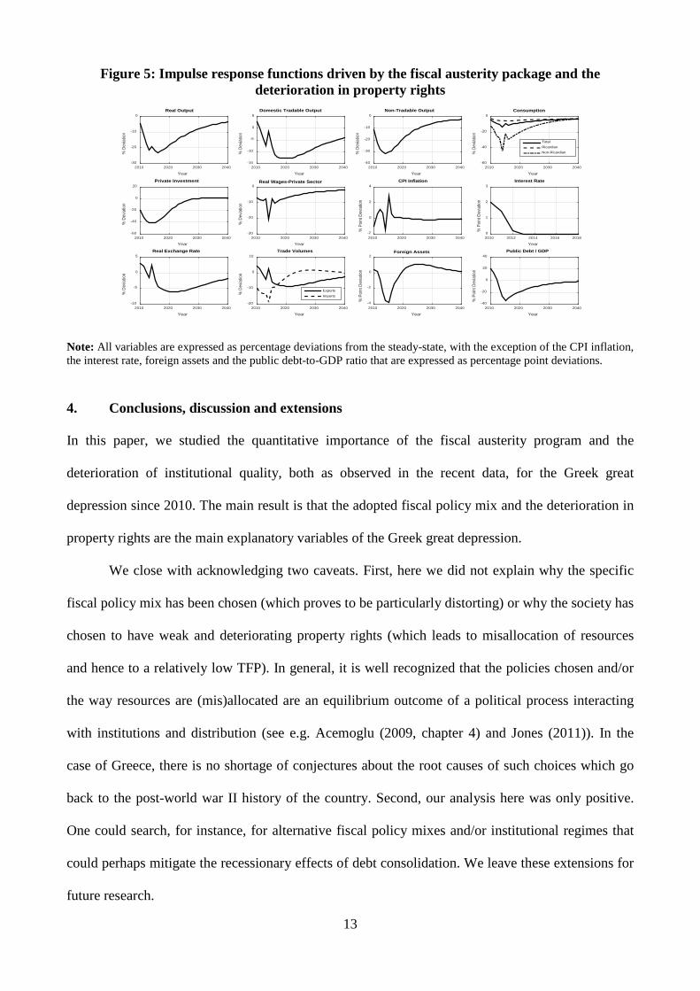
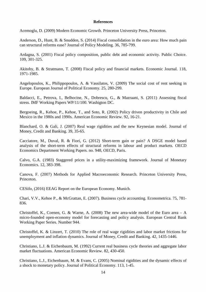
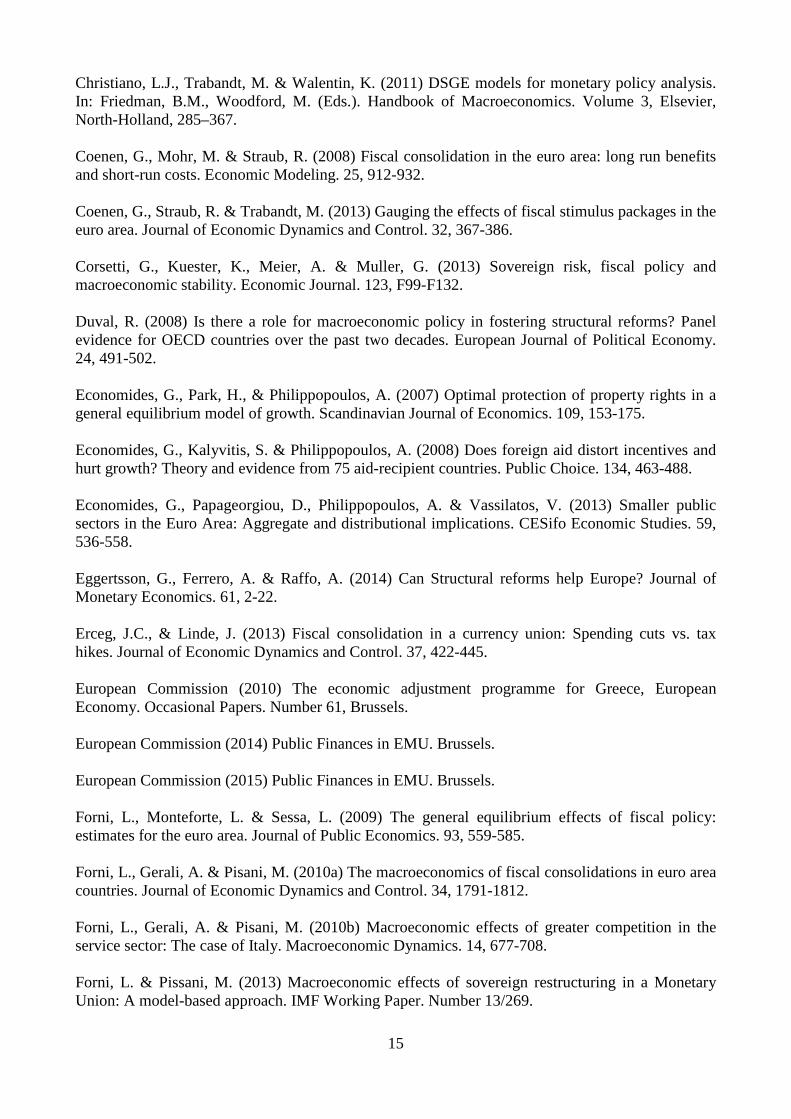
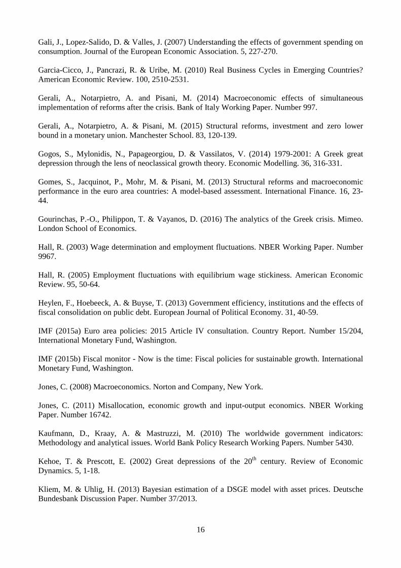
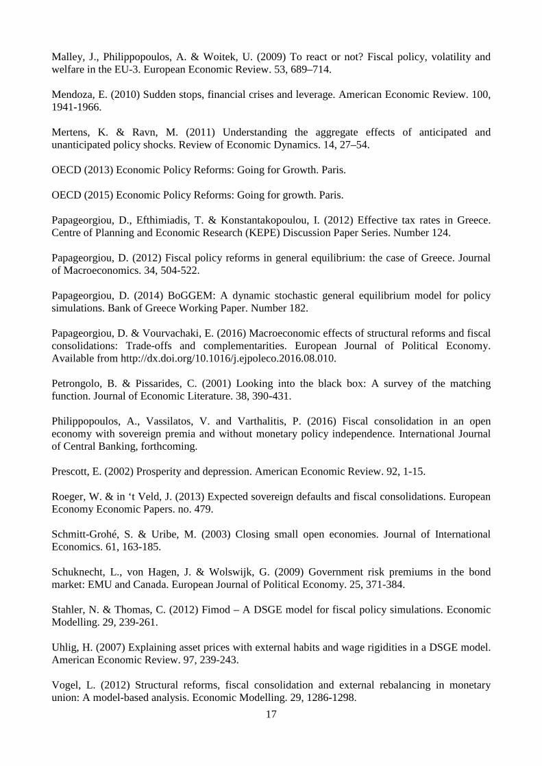
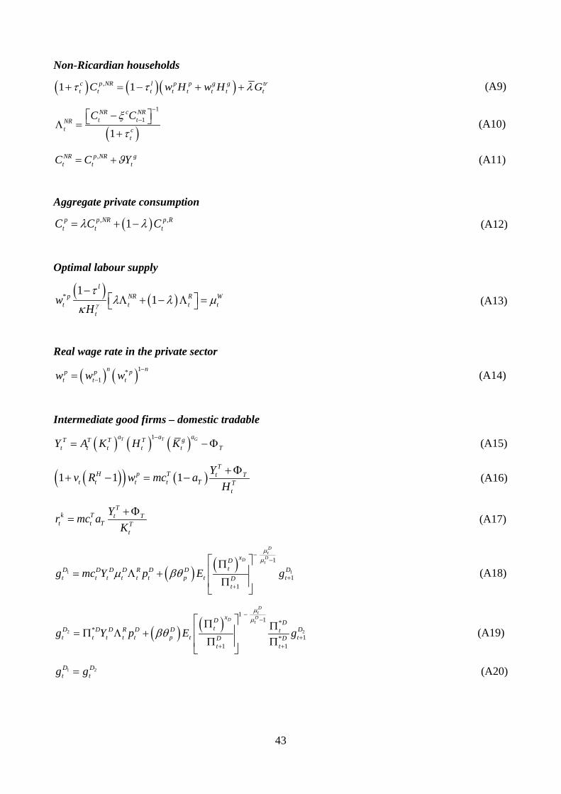
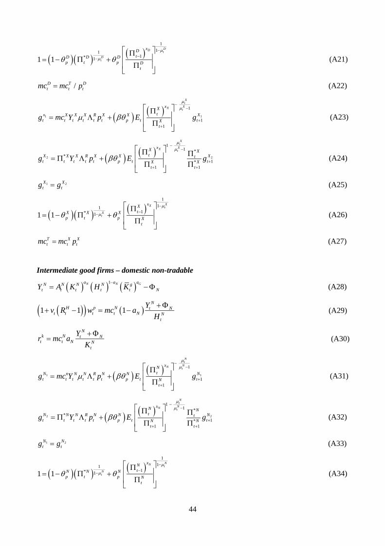
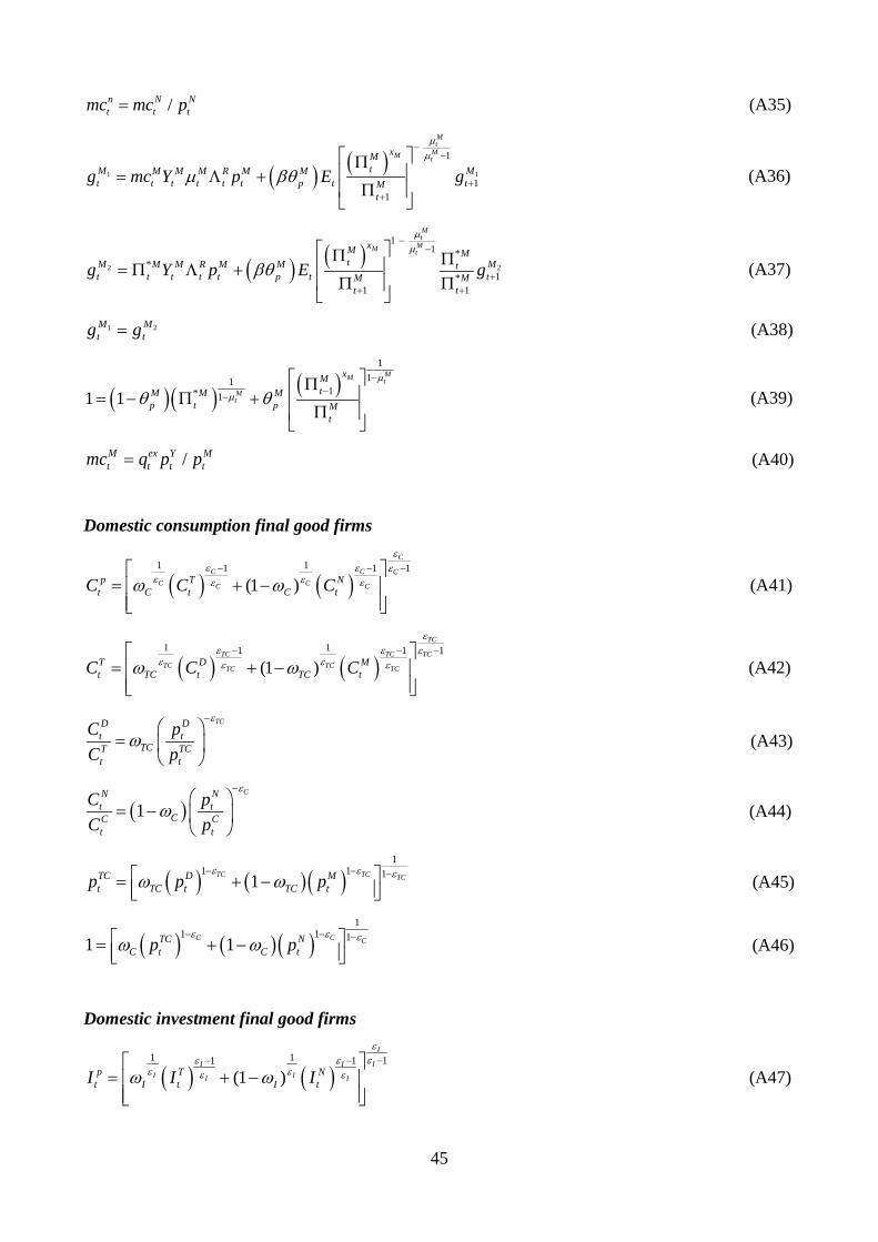
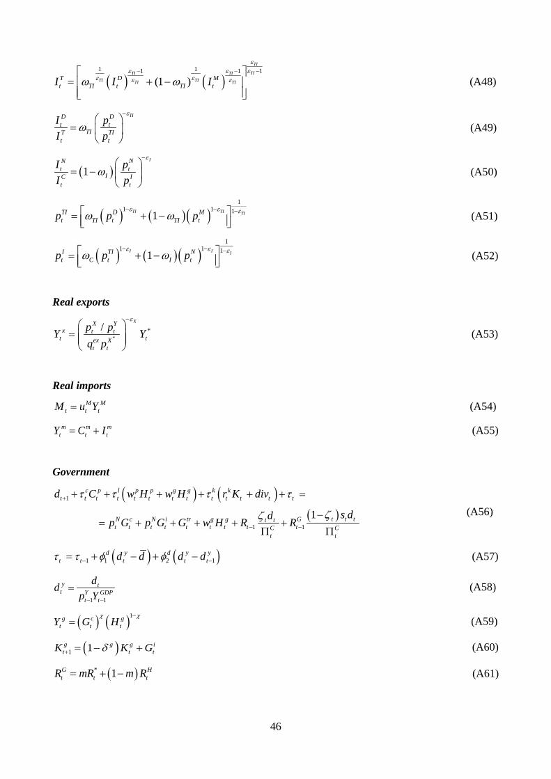
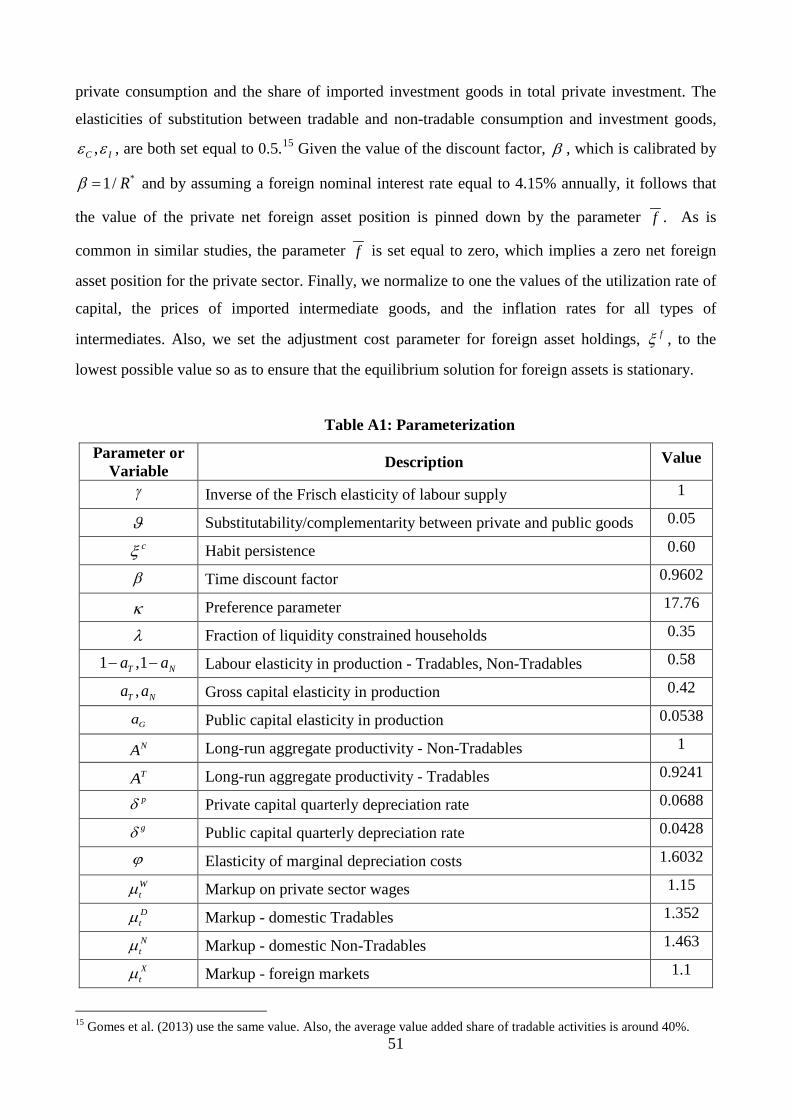
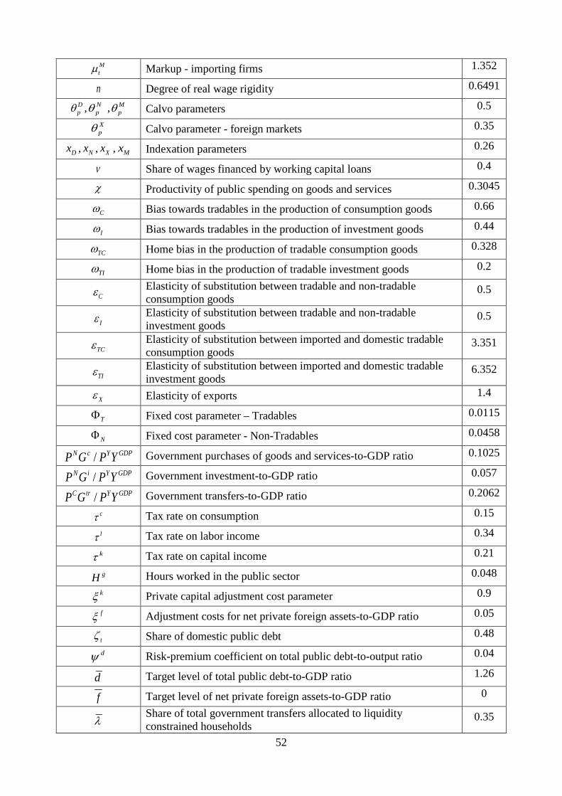
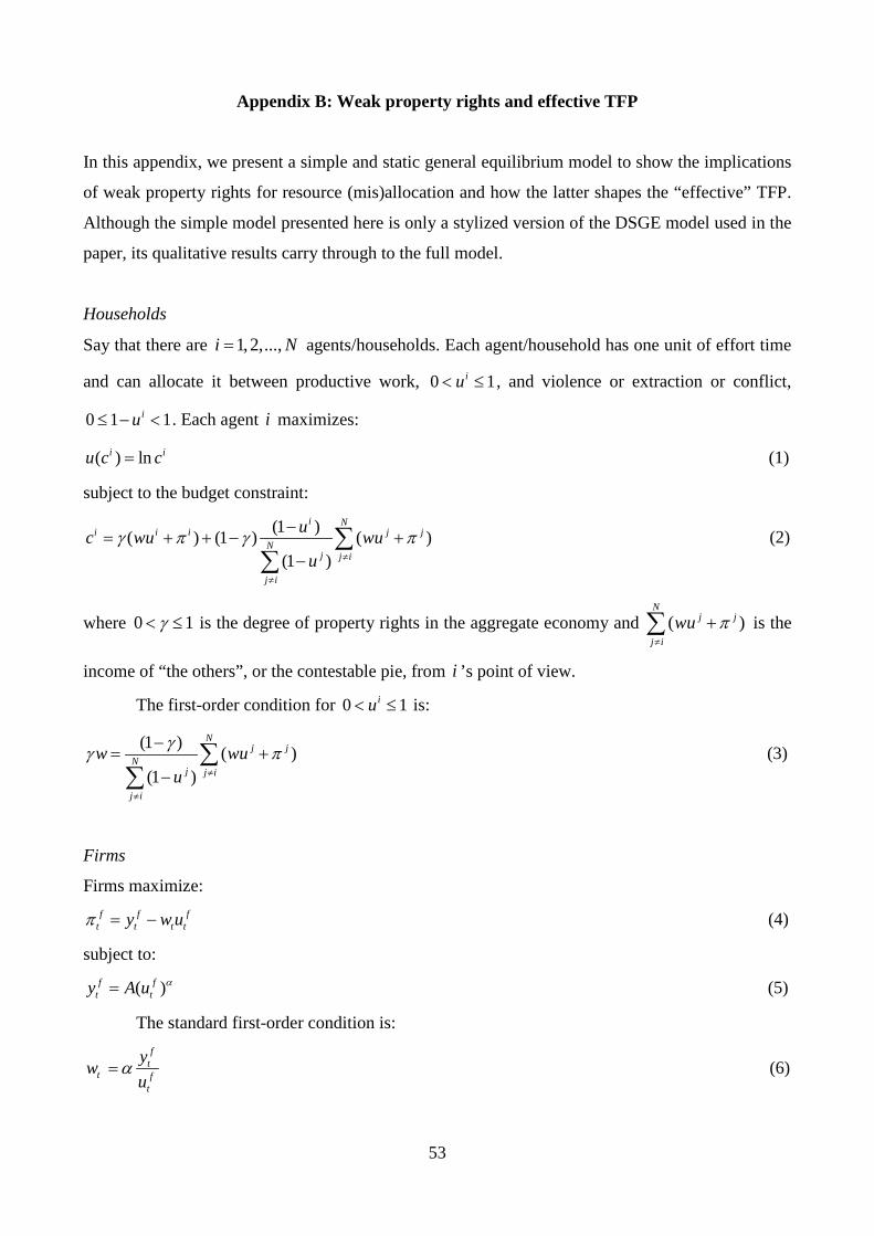
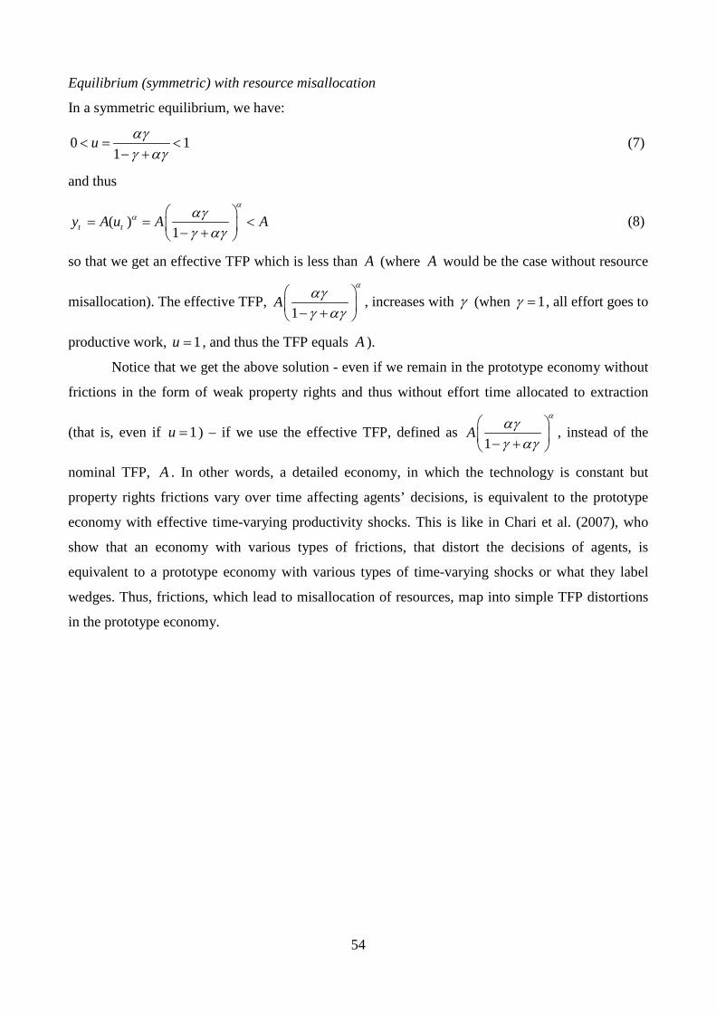