Viele Wege führen zu π - MathWorks - Makers of … Wege führen zu π Von Cleve Moler Die...
4
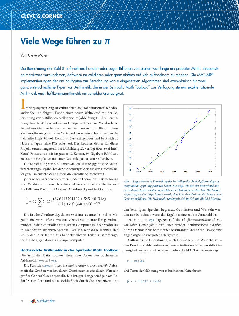
1 CLEVE’S CORNER Viele Wege führen zu π Von Cleve Moler Die Berechnung der Zahl π auf mehrere hundert oder sogar Billionen von Stellen war lange ein probates Mittel, Stresstests an Hardware vorzunehmen, Software zu validieren oder ganz einfach auf sich aufmerksam zu machen. Die MATLAB ® - Implementierungen der am häufigsten zur Berechnung von π eingesetzten Algorithmen sind exemplarisch für zwei ganz unterschiedliche Typen von Arithmetik, die in der Symbolic Math Toolbox ™ zur Verfügung stehen: exakte rationale Arithmetik und Fließkommaarithmetik mit variabler Genauigkeit. I m vergangenen August verkündeten die Hobbyinformatiker Alex- ander Yee und Shigeru Kondo einen neuen Weltrekord mit der Be- stimmung von 5 Billionen Stellen von π (Abbildung 1). Ihre Berech- nung dauerte 90 Tage auf einem Computer-Eigenbau. Yee absolviert derzeit ein Graduiertenstudium an der University of Illinois. Seine Rechensoſtware „y-cruncher“ entstand aus einem Schulprojekt an der Palo Alto High School. Kondo ist Systemingenieur und baut sich zu Hause in Japan seine PCs selbst auf. Der Rechner, den er für dieses Projekt zusammengestellt hat (Abbildung 2), verfügt über zwei Intel® Xeon®-Prozessoren mit insgesamt 12 Kernen, 96 Gigabyte RAM und 20 externe Festplatten mit einer Gesamtkapazität von 32 Terabyte. Die Berechnung von 5 Billionen Stellen ist eine gigantische Daten- verarbeitungsaufgabe, bei der die benötigte Zeit für den Datentrans- fer genauso entscheidend ist wie die eigentliche Rechenzeit. y-cruncher nutzt mehrere verschiedene Formeln zur Berechnung und Verifikation. Sein Herzstück ist eine eindrucksvolle Formel, die 1987 von David und Gregory Chudnovsky entdeckt wurde: Die Brüder Chudnovsky, denen zwei interessante Artikel im Ma- gazin e New Yorker sowie ein NOVA-Dokumentarfilm gewidmet wurden, haben ebenfalls ihre eigenen Computer in ihrer Wohnung in Manhattan zusammengebaut. Der Massenparallelrechner, den sie in den 90er Jahren aus handelsüblichen Teilen zusammenge- stellt haben, galt damals als Supercomputer. Hochexakte Arithmetik in der Symbolic Math Toolbox Die Symbolic Math Toolbox bietet zwei Arten von hochexakter Arithmetik: sym und vpa. Die Funktion sym initiiert die exakte rationale Arithmetik: Arith- metische Größen werden durch Quotienten sowie durch Wurzeln großer Ganzzahlen dargestellt. Die Integer-Länge wird je nach Be- darf vergrößert und ist ausschließlich durch die Rechenzeit und den benötigten Speicher begrenzt. Quotienten und Wurzeln wer- den nur berechnet, wenn das Ergebnis eine exakte Ganzzahl ist. Die Funktion vpa dagegen ruſt die Fließkommaarithmetik mit variabler Genauigkeit auf: Hier werden arithmetische Größen durch Dezimalbrüche mit einer bestimmten Stellenzahl sowie eine angehängte Zehnerpotenz dargestellt. Arithmetische Operationen, auch Divisionen und Wurzeln, kön- nen Rundungsfehler aufweisen, deren Größe durch die gewählte Ge- nauigkeit bestimmt ist. So erzeugt etwa die MATLAB-Anweisung p = rat(pi) drei Terme der Näherung von π durch einen Kettenbruch p = 3 + 1/(7 + 1/16) Abb. 1: Logarithmische Darstellung der im Wikipedia-Artikel „Chronology of computation of pi“ aufgelisteten Daten. Sie zeigt, wie sich der Weltrekord der Anzahl berechneter Stellen in den letzten 60 Jahren entwickelt hat. Die lineare Anpassung an den Logarithmus verrät, dass hier eine Variante des Mooreschen Gesetzes erfüllt ist. Die Stellenzahl verdoppelt sich im Schnitt alle 22,5 Monate.
-
Upload
nguyenminh -
Category
Documents
-
view
228 -
download
0
Transcript of Viele Wege führen zu π - MathWorks - Makers of … Wege führen zu π Von Cleve Moler Die...
1
CLEVE’S CORNER
Viele Wege führen zu πVon Cleve Moler
Die Berechnung der Zahl π auf mehrere hundert oder sogar Billionen von Stellen war lange ein probates Mittel, Stresstests
an Hardware vorzunehmen, Software zu validieren oder ganz einfach auf sich aufmerksam zu machen. Die MATLAB®-
Implementierungen der am häufigsten zur Berechnung von π eingesetzten Algorithmen sind exemplarisch für zwei
ganz unterschiedliche Typen von Arithmetik, die in der Symbolic Math Toolbox™ zur Verfügung stehen: exakte rationale
Arithmetik und Fließkommaarithmetik mit variabler Genauigkeit.
Im vergangenen August verkündeten die Hobbyinformatiker Alexander Yee und Shigeru Kondo einen neuen Weltrekord mit der Bestimmung von 5 Billionen Stellen von π (Abbildung 1). Ihre Berechnung dauerte 90 Tage auf einem ComputerEigenbau. Yee absolviert derzeit ein Graduiertenstudium an der University of Illinois. Seine Rechensoftware „ycruncher“ entstand aus einem Schulprojekt an der Palo Alto High School. Kondo ist Systemingenieur und baut sich zu Hause in Japan seine PCs selbst auf. Der Rechner, den er für dieses Projekt zusammengestellt hat (Abbildung 2), verfügt über zwei Intel® Xeon®Prozessoren mit insgesamt 12 Kernen, 96 Gigabyte RAM und 20 externe Festplatten mit einer Gesamtkapazität von 32 Terabyte.
Die Berechnung von 5 Billionen Stellen ist eine gigantische Datenverarbeitungsaufgabe, bei der die benötigte Zeit für den Datentransfer genauso entscheidend ist wie die eigentliche Rechenzeit.
ycruncher nutzt mehrere verschiedene Formeln zur Berechnung und Verifikation. Sein Herzstück ist eine eindrucksvolle Formel, die 1987 von David und Gregory Chudnovsky entdeckt wurde:
Cleve's Corner: Computing π Computing hundreds, or trillions, of digits of π has long been used to stress hardware, validate software, and establish bragging rights. MATLAB implementations of the most widely used algorithms for computing π illustrate two different styles of arithmetic available in Symbolic Math Toolbox: exact rational arithmetic and variable-precision floating-point arithmetic.
Last August, two computer hobbyists, Alexander Yee and Shigeru Kondo, announced that they had set a world record by computing five trillion digits of π. Their computation took 90 days on a homebrew PC. Yee is now a graduate student at the University of Illinois. His computing software, “y-cruncher”, began as a class project at Palo Alto High School. Kondo is a systems engineer who assembles personal computers at his home in Japan. The machine that he built for this project (Figure 1) has two Intel Xeons with a total of 12 cores, 96 gigabytes of RAM, and 20 external hard disks with a combined capacity of 32 terabytes.
The computation of five trillion digits is a huge processing task where the time required for the data movement is just as important as the time required for the arithmetic.
y-cruncher uses several different formulas for computation and verification. The primary tool is a formidable formula discovered by David and Gregory Chudnovsky in 1987.
The Chudnovsky brothers, who were the subject of two fascinating articles in the New Yorker and a NOVA documentary, have also built “home brew” computers in their apartment in Manhattan. The massively parallel machine that they assembled from commodity parts in the 1990s was considered a supercomputer at the time.
High-Precision Arithmetic in Symbolic Math Toolbox
Symbolic Math Toolbox provides two styles of high-precision arithmetic, sym and vpa.
The sym function initiates exact rational arithmetic: Arithmetic quantities are represented by quotients and roots of large integers. Integer length increases as necessary, limited only by computer time and storage requirements. Quotients and roots are not computed unless the result is an exact integer.
The vpa function initiates variable-precision floating-point arithmetic: Arithmetic quantities are represented by decimal fractions of a specified length together with a power-of-ten exponent.
Arithmetic operations, including divisions and roots, can involve roundoff errors at the level of the specified accuracy.For example, the MATLAB statement
p = rat(pi)
Die Brüder Chudnovsky, denen zwei interessante Artikel im Magazin The New Yorker sowie ein NOVA-Dokumentarfilm gewidmet wurden, haben ebenfalls ihre eigenen Computer in ihrer Wohnung in Manhattan zusammengebaut. Der Massenparallelrechner, den sie in den 90er Jahren aus handelsüblichen Teilen zusammengestellt haben, galt damals als Supercomputer.
Hochexakte Arithmetik in der Symbolic Math Toolbox Die Symbolic Math Toolbox bietet zwei Arten von hochexakter Arithmetik: sym und vpa.
Die Funktion sym initiiert die exakte rationale Arithmetik: Arithmetische Größen werden durch Quotienten sowie durch Wurzeln großer Ganzzahlen dargestellt. Die IntegerLänge wird je nach Bedarf vergrößert und ist ausschließlich durch die Rechenzeit und
den benötigten Speicher begrenzt. Quotienten und Wurzeln werden nur berechnet, wenn das Ergebnis eine exakte Ganzzahl ist.
Die Funktion vpa dagegen ruft die Fließkommaarithmetik mit variabler Genauigkeit auf: Hier werden arithmetische Größen durch Dezimalbrüche mit einer bestimmten Stellenzahl sowie eine angehängte Zehnerpotenz dargestellt.
Arithmetische Operationen, auch Divisionen und Wurzeln, können Rundungsfehler aufweisen, deren Größe durch die gewählte Genauigkeit bestimmt ist. So erzeugt etwa die MATLABAnweisung
p = rat(pi)
drei Terme der Näherung von π durch einen Kettenbruch
p = 3 + 1/(7 + 1/16)
Abb. 1: Logarithmische Darstellung der im Wikipedia-Artikel „Chronology of computation of pi“ aufgelisteten Daten. Sie zeigt, wie sich der Weltrekord der Anzahl berechneter Stellen in den letzten 60 Jahren entwickelt hat. Die lineare Anpassung an den Logarithmus verrät, dass hier eine Variante des Mooreschen Gesetzes erfüllt ist. Die Stellenzahl verdoppelt sich im Schnitt alle 22,5 Monate.

2
Die Anweisung
sym(p)
liefert danach den rationalen Ausdruck
355/113
der eine reizvolle Alternative zum sonst üblichen Bruch 22/7 darstellt. Dagegen ergibt die Anweisung
vpa(p,8)
den achtstelligen Fließkommawert
3,1415929
Der Chudnovsky-Algorithmus Die vorstehenden MATLABProgramme implementieren nur drei aus hunderten möglicher Algorithmen zur Berechnung von π. Der ChudnovskyAlgorithmus (Abbildung 3) bedient sich bis auf den letzten Schritt der exakten rationalen Arithmetik. Jeder Ausdruck der ChudnovskyReihe liefert etwa 14 Dezimalstellen, d. h. um d Stellen zu erhalten, benötigt man [d/14] Ausdrücke. Die Anweisung
chud_pi(42)
erzeugt beispielsweise durch exakte rationale Berechnung
produces three terms in the continued fraction approximation of π
p = 3 + 1/(7 + 1/16)
Then the statement
sym(p)
yields the rational expression
355/113
which is an attractive alternative to the familiar 22/7. On the other hand, the statement
vpa(p,8)
produces the 8-digit floating-point value
3.1415929
The Chudnovsky Algorithm
Our MATLAB programs implement three of the hundreds of possible algorithms for computing π. The Chudnovsky algorithm (Figure 2) uses exact rational arithmetic until the last step. Each term in the Chudnovsky series provides about 14 decimal digits, so to obtain d digits requires terms. For example, the statement
chud_pi(42) uses exact rational computation to produce
and then the final step uses variable-precision floating-point arithmetic with 42 digits to produce
3.14159265358979323846264338327950288419717
One interesting fact about the digits of π is revealed by
chud_pi(775)
or
vpa(pi,775)
Der letzte Schritt erzeugt dann mithilfe von Fließkommaarithmetik mit variabler Genauigkeit das 42stellige Ergebnis
3,14159265358979323846264338327950288419717
Eine interessante Besonderheit in den Ziffern von π offenbart sich durch
chud_pi(775)
oder
vpa(pi,775)
Beide erzeugen 775 Stellen, die jeweils anfangen und enden mit:
3,141592653589793238 ...... 707211349999998372978
Wir erkennen hier nicht nur, dass chud_pi korrekt arbeitet, sondern auch, dass um die Position 765 in der Dezimalentwicklung von π sechsmal hintereinander die Ziffer 9 erscheint (Abbildung 4).
Die Berechnung von 5000 Stellen mit chud_pi erfordert 358 Ausdrücke und dauert auf meinem Laptop ungefähr 20 Sekunden. Der dabei erzeugte symbolische Ausdruck enthält 12.425 Zeichen.
Abb. 2: Shigeru Kondos Eigenbau-PC, der derzeit den Weltrekord der berechneten Stellen von π hält.
Abb. 3: MATLAB-Implementierung des Chudnovsky-Algorithmus. sym initiiert darin die exakte rationale Arithmetik.
function P = chud _ pi(d)
% CHUD _ PI Chudnovsky algorithm for pi.
% chud _ pi(d) produces d decimal digits.
k = sym(0);
s = sym(0);
sig = sym(1);
n = ceil(d/14);
for j = 1:n
s = s + sig * prod(3*k+1:6*k)/prod(1:k)̂ 3 * ...
(13591409+545140134*k) / 640320 (̂3*k+3/2);
k = k+1;
sig = -sig;
end
S = 1/(12*s);
P = vpa(S,d);
3
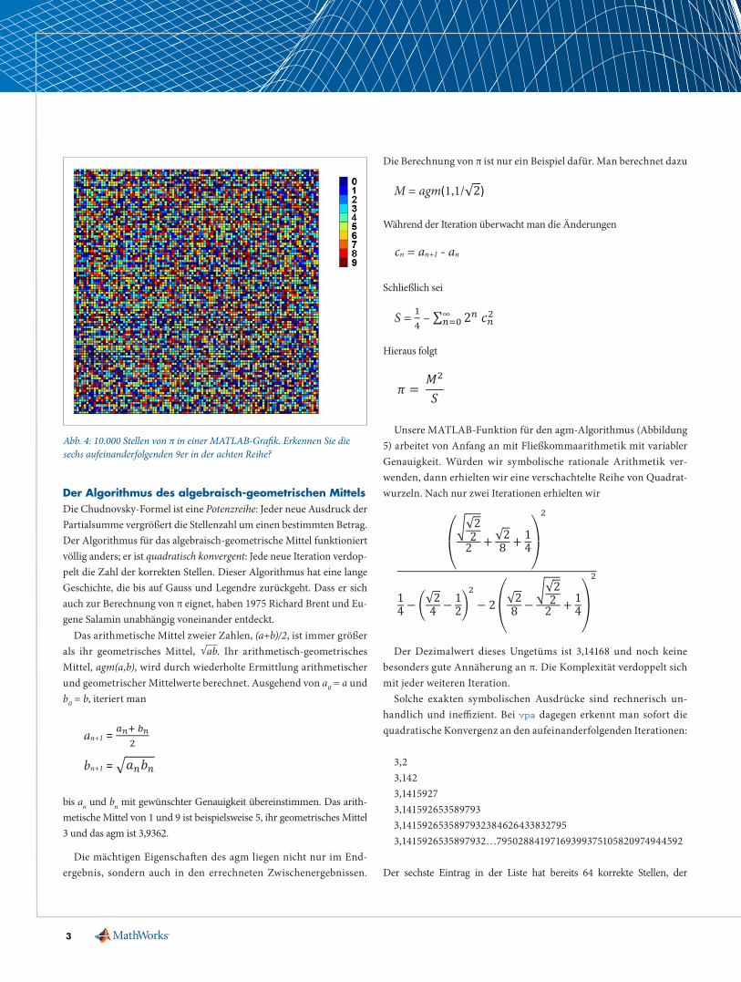
Der Algorithmus des algebraisch-geometrischen MittelsDie ChudnovskyFormel ist eine Potenzreihe: Jeder neue Ausdruck der Partialsumme vergrößert die Stellenzahl um einen bestimmten Betrag. Der Algorithmus für das algebraischgeometrische Mittel funktioniert völlig anders; er ist quadratisch konvergent: Jede neue Iteration verdoppelt die Zahl der korrekten Stellen. Dieser Algorithmus hat eine lange Geschichte, die bis auf Gauss und Legendre zurückgeht. Dass er sich auch zur Berechnung von π eignet, haben 1975 Richard Brent und Eugene Salamin unabhängig voneinander entdeckt.
Das arithmetische Mittel zweier Zahlen, (a+b)/2, ist immer größer als ihr geometrisches Mittel, √ab. Ihr arithmetischgeometrisches Mittel, agm(a,b), wird durch wiederholte Ermittlung arithmetischer und geometrischer Mittelwerte berechnet. Ausgehend von a0 = a und b0 = b, iteriert man
bis an und bn mit gewünschter Genauigkeit übereinstimmen. Das arithmetische Mittel von 1 und 9 ist beispielsweise 5, ihr geometrisches Mittel 3 und das agm ist 3,9362.
Die mächtigen Eigenschaften des agm liegen nicht nur im Endergebnis, sondern auch in den errechneten Zwischenergebnissen.
Abb. 4: 10.000 Stellen von π in einer MATLAB-Grafik. Erkennen Sie die sechs aufeinanderfolgenden 9er in der achten Reihe?
Die Berechnung von π ist nur ein Beispiel dafür. Man berechnet dazu
Während der Iteration überwacht man die Änderungen
Schließlich sei
Hieraus folgt
Unsere MATLABFunktion für den agmAlgorithmus (Abbildung 5) arbeitet von Anfang an mit Fließkommaarithmetik mit variabler Genauigkeit. Würden wir symbolische rationale Arithmetik verwenden, dann erhielten wir eine verschachtelte Reihe von Quadratwurzeln. Nach nur zwei Iterationen erhielten wir
Our MATLAB function for the agm algorithm (Figure 3) uses variable- precision floating-point arithmetic from the very beginning. If we used symbolic rational arithmetic, we would end up with a nested sequence of square roots. After just two iterations we would have
The decimal value of this monstrosity is 3.14168, so it is not yet a very good approximation to . The complexity doubles with each iteration.
Such exact symbolic expressions are computationally unwieldy and inefficient. With vpa, however, the quadratic convergence can be seen in the successive iterates:
3.2 3.142 3.1415927 3.141592653589793 3.1415926535897932384626433832795 3.141592653589793238462643383279502884197169399375105820974944592 The tenth entry is this output would have 1024 correct digits.
The quadratic convergence makes agm very fast. To compute 100,000 digits requires only 17 steps and about 2.5 seconds on my laptop.
The BBP Formula
Yee spot-checked his computation with the BBP formula. This formula, named after David Bailey, Jonathan Borwein, and Simon Plouffe and discovered by Plouffe in 1995, is a power series involving inverse powers of 16.
Der Dezimalwert dieses Ungetüms ist 3,14168 und noch keine besonders gute Annäherung an π. Die Komplexität verdoppelt sich mit jeder weiteren Iteration.
Solche exakten symbolischen Ausdrücke sind rechnerisch unhandlich und ineffizient. Bei vpa dagegen erkennt man sofort die quadratische Konvergenz an den aufeinanderfolgenden Iterationen:
3,23,1423,14159273,1415926535897933,14159265358979323846264338327953,1415926535897932…79502884197169399375105820974944592
Der sechste Eintrag in der Liste hat bereits 64 korrekte Stellen, der
These both produce 775 digits, beginning and ending with
3.141592653589793238 ...... 707211349999998372978
We see not only that chud_pi is working correctly but also that there are six 9s in a row around position 765 in the decimal expansion of π (Figure 4).
Computing five thousand digits with chud_pi requires 358 terms and takes about 20 seconds on my laptop. The final symbolic expression contains 12,425 characters.
The Algebraic-Geometric Mean Algorithm
The Chudnovsky formula is a power series: Each new term in the partial sum adds a fixed number of digits of accuracy. The algebraic-geometric mean algorithm is completely different; it is quadratically convergent: Each new iteration doubles the number of correct digits. The agm algorithm has a long history dating back to Gauss and Legendre. Its ability to compute π was discovered independently by Richard Brent and Eugene Salamin in 1975.
The arithmetic mean of two numbers, (a+b)/2, is always greater than their geometric mean, √𝑎𝑎𝑎𝑎. Their arithmetic-geometric mean, or agm(a,b), is computed by repeatedly taking arithmetic and geometric means. Starting with a0 = a and b0 = b, iterate
an+1 = 𝑎𝑎𝑛𝑛+ 𝑏𝑏𝑛𝑛2
bn+1 = �𝑎𝑎𝑛𝑛𝑎𝑎𝑛𝑛
until an and bn agree to a desired accuracy. For example, the arithmetic mean of 1 and 9 is 5, the geometric mean is 3, and the agm is 3.9362.
The powerful properties of the agm lie not just in the final value but also in the results generated along the way. Computing π is just one example. It involves computing
M = agm(1,1/√2)
During the iteration, keep track of the changes,
cn = an+1 - an
Finally, let
S = 14 – ∑ 2𝑛𝑛∞
𝑛𝑛=0 𝑐𝑐𝑛𝑛2
Then
𝜋𝜋 = 𝑀𝑀2
𝑆𝑆
Our MATLAB function for the agm algorithm (Figure 3) uses variable- precision floating-point arithmetic from the very beginning. If we used symbolic rational arithmetic, we would end up with a nested sequence of square roots. After just two iterations we would have
⎝
⎛�√2
22 + √2
8 + 14⎠
⎞
2
14 − �√2
4 − 12�
2
− 2
⎝
⎛√28 −
�√22
2 + 14⎠
⎞
2
The decimal value of this monstrosity is 3.14168, so it is not yet a very good approximation to 𝜋𝜋. The complexity doubles with each iteration.
Such exact symbolic expressions are computationally unwieldy and inefficient. With vpa, however, the quadratic convergence can be seen in the successive iterates:
3.2 3.142
4
Download: MATLAB-Implementierungen der Chudnovsky-, agm- und BBP-Algorithmenwww.mathworks.de/computing-pi
Cleve's Corner Collection www.mathworks.de/clevescorner
Weitere Informationen
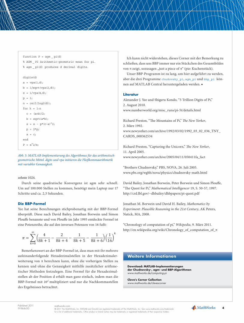
Abb. 5: MATLAB-Implementierung des Algorithmus für das arithmetisch-geometrische Mittel. digits und vpa initiieren die Fließkommaarithmetik mit variabler Genauigkeit.
function P = agm _ pi(d)
% AGM _ PI Arithmetic-geometric mean for pi.
% agm _ pi(d) produces d decimal digits.
digits(d)
a = vpa(1,d);
b = 1/sqrt(vpa(2,d));
s = 1/vpa(4,d);
p = 1;
n = ceil(log2(d));
for k = 1:n
c = (a+b)/2;
b = sqrt(a*b);
s = s - p*(c-a)̂ 2;
p = 2*p;
a = c;
end
P = a^2/s;
Ich kann nicht widerstehen, dieses Corner mit der Bemerkung zu schließen, dass uns BBP immer nur ein Stückchen des Gesamtbildes von π zeigt, sozusagen „just a piece of π“ (pie: Kuchenstück).
Unser BBPProgramm ist zu lang, um hier aufgeführt zu werden, aber die drei Programme chudovsky_pi, agm_pi und bbp_pi können auf MATLAB Central heruntergeladen werden. ■
Literatur Alexander J. Yee und Shigeru Kondo, “5 Trillion Digits of Pi,” 2. August 2010.www.numberworld.org/misc_runs/pi5t/details.html
Richard Preston, “The Mountains of Pi,” The New Yorker, 2. März 1992.www.newyorker.com/archive/1992/03/02/1992_03_02_036_TNY_CARDS_000362534
Richard Preston, “Capturing the Unicorn,” The New Yorker, 11. April 2005.www.newyorker.com/archive/2005/04/11/050411fa_fact
“Brothers Chudnovsky,” PBS, NOVA, 26. Juli 2005.www.pbs.org/wgbh/nova/physics/chudnovskymath.html
David Bailey, Jonathan Borwein, Peter Borwein und Simon Plouffe, “The Quest for Pi,” Mathematical Intelligencer 19, S. 5057, 1997.http://crd.lbl.gov/~dhbailey/dhbpapers/piquest.pdf
Jonathan M. Borwein und David H. Bailey, Mathematics by Experiment: Plausible Reasoning in the 21st Century, AK Peters, Natick, MA, 2008.
“Chronology of computation of pi,” Wikipedia, 9. März 2011.http://en.wikipedia.org/wiki/Chronology_of_computation_of_π
zehnte 1024.Durch seine quadratische Konvergenz ist agm sehr schnell.
Um auf 100.000 Stellen zu kommen, benötigt mein Laptop nur 17 Schritte und ca. 2,5 Sekunden.
Die BBP-FormelYee hat seine Berechnungen stichprobenartig mit der BBPFormel überprüft. Diese nach David Bailey, Jonathan Borwein und Simon Plouffe benannte und von Plouffe im Jahr 1995 entdeckte Formel ist eine Potenzreihe, die auf den inversen Potenzen von 16 fußt:
Our MATLAB function for the agm algorithm (Figure 3) uses variable- precision floating-point arithmetic from the very beginning. If we used symbolic rational arithmetic, we would end up with a nested sequence of square roots. After just two iterations we would have
The decimal value of this monstrosity is 3.14168, so it is not yet a very good approximation to . The complexity doubles with each iteration.
Such exact symbolic expressions are computationally unwieldy and inefficient. With vpa, however, the quadratic convergence can be seen in the successive iterates:
3.2 3.142 3.1415927 3.141592653589793 3.1415926535897932384626433832795 3.141592653589793238462643383279502884197169399375105820974944592 The tenth entry is this output would have 1024 correct digits.
The quadratic convergence makes agm very fast. To compute 100,000 digits requires only 17 steps and about 2.5 seconds on my laptop.
The BBP Formula
Yee spot-checked his computation with the BBP formula. This formula, named after David Bailey, Jonathan Borwein, and Simon Plouffe and discovered by Plouffe in 1995, is a power series involving inverse powers of 16.
Bemerkenswert an der BBPFormel ist, dass man mit ihr mehrere aufeinanderfolgende Hexadezimalstellen in der Hexadezimalerweiterung von π berechnen kann, ohne die vorherigen Stellen zu kennen und ohne die Genauigkeit mithilfe zusätzlicher arithmetischer Methoden festzulegen. Eine Formel für die Hexadezimalstellen ab der Position d erhält man ganz einfach, indem man die BBPFormel mit 16d multipliziert und nur die Nachkommastellen des Ergebnisses betrachtet.
Weitere Informationen
mathworks.com© 2011 The MathWorks, Inc. MATLAB and Simulink are registered trademarks of The MathWorks, Inc. See www.mathworks.com/trademarks for a list of additional trademarks. Other product or brand names may be trademarks or registered trademarks of their respective holders.
Published 2011 91964v00


![Neue Wege in der Entzündungsdiagnostik · *] Mi t Unterstützung durch die DFG, Ho 781 /3-3 und des Sonderforschungsbereichs (Universität München) 207, LP 8 Einleitung Trotz intensiver](https://static.fdocument.org/doc/165x107/5e045f83c060076a3b023459/neue-wege-in-der-entzndungsdiagnostik-mi-t-untersttzung-durch-die-dfg-ho.jpg)