V. Parkhomchuk I. Ben-Zvi - Brookhaven National Laboratory · · 2013-01-292/ρ2 ×2 ρ/V. The...

C-A/AP/47April 2001

Electron Cooling for RHIC

V. ParkhomchukBudker Institute of Nuclear Physics

I. Ben-ZviBrookhaven National Laboratory

Collider-Accelerator DepartmentBrookhaven National Laboratory

Upton, NY 11973

ELECTRON COOLING

FOR RHIC

Review of the Principles ofElectron Cooling for the

Relativistic Heavy Ion Collider (RHIC)

Principal Investigators:

Vasily [email protected]

Budker Institute of Nuclear Physics,Novosibirsk, 630090

Ilan [email protected]

Collider-Accelerator DepartmentAnd

National Synchrotron Light SourceBrookhaven National Laboratory

Upton NY 11973-5000

mailto:[email protected]

mailto:[email protected]

2

ELECTRON COOLING FORRHIC

ContentsINTRODUCTION............................................................................................................... 4

I.1 RHIC Gold-on-Gold collider parameters............................................................ 4I.2 Main features of electron cooling for heavy ion ................................................. 5

1 MAIN SCENARIO FOR ELECTRON COOLING....................................................... 101.1. Continuous cooling at the collider’s storage energy ......................................... 101.2. Cooling at beam injection energy...................................................................... 17Conclusions for the cooling scenario section................................................................ 19

2. LUMINOSITY UNDER COOLING ............................................................................ 202.1 Beam Parameters at the Interaction Points........................................................ 202.2. Beam-beam interaction ..................................................................................... 202.3 Noise and beam-beam ....................................................................................... 222.4 Simulation of beam-beam effects for the gold ion collisions at RHIC. ............ 222.5 Recombination and dissociation ion losses....................................................... 26

3. THE TECHNICAL APPROACH FOR THE ELECTRON COOLING SYSTEM...... 293.1 The parameters of the cooling electron beam ................................................... 29

3.1.1 Cooling section length.............................................................................. 293.1.2 Electron Beam Parameters .................................................................... 31

3.2 Schematic layout of the cooling system next to a RHIC interaction point ....... 313.3. Electron gun in DC accelerator (2 MeV). ......................................................... 373.4. Bunching system ............................................................................................... 393.5 Main linac.......................................................................................................... 463.6 Debunching system after linac. ......................................................................... 503.7. Injection of the electron beam into the field of solenoid................................... 51

3.7.1. Injection of a flat electron beam using quadrupoles. ................................ 513.7.2. Injection of round electron beam generated by a magnetized cathode ..... 56

3.8. Cooling straight section parameters .................................................................. 583.8.1. The effect of gap between sections of the main solenoid. ........................ 593.8.2. Choice of section length. ........................................................................... 603.8.3. A coil for the compensation of the gap effect. .......................................... 613.8.4. A coil for the correction of the magnetic field error. ................................ 63

3.9 Recuperating the energy of the electron beam in the main linac ...................... 653.10 Recuperating the energy of the electron beam in the DC accelerator ............... 66

4. KEY-PHYSICAL PROCESSES................................................................................... 674.1 The drag force in the absence of a magnetic field................................................. 674.2 The drag force in a magnetic field ........................................................................ 684.3 Stationary parameters of an ion beam after cooling.............................................. 714.4 The space charge tune shift (Laslett tune shift)..................................................... 72

3

4.5 The Intra Beam Scattering..................................................................................... 734.6 Ion beam loss rate by capture of electrons at cooler ......................................... 754.7 Noise and growth of the ion beam emittance......................................................... 774.8 Requirement on impedance after cooling............................................................... 78

5. COLLECTIVE EFFECTS............................................................................................. 805.1 Laslett tune shift ................................................................................................ 805.2. Electron-beam ion interaction problems ................................................................ 80

5.2.1 The longitudinal-longitudinal coherent interaction................................... 805.2.2. The transverse-longitudinal coherent interaction...................................... 82

6. CONTROL OF THE ION BEAM DISTRIBUTION IN 6-D PHASE-SPACE............ 847. STOCHASTIC COOLING SYSTEM. ......................................................................... 888. CONSIDERATIONS TOWARDS A CDR .................................................................. 95

4

INTRODUCTION I.1 RHIC Gold-on-Gold collider parameters

The development of nuclear physics experimental research resulted in a sharpincrease in the requirements for particle-beam quality. It is especially important to obtainbeams of high density and low momentum spread. The luminosity of a collider isdetermined by the emittance ε of the bunches, the number of particles in the bunch Ni, thebeta function at the interaction point βIP, and the bunch repetition frequency fb as

b

IP

ii fNN

Lπεβ4

×= . (1)

Cooling helps decrease the beam emittance, and decreasing the momentum spread ∆p/phelps to achieve stronger focusing and smaller βIP. Without any cooling the normalizedemittance of the ion beam increases by dilution at nonlinear elements of the transverseand longitudinal optics during injection and acceleration. If the ion source does not havea high brightness, it is impossible to reach maximal luminosity. For a luminosity limitedby the beam-beam effect at the collision points equation (1) can be rewritten in the form:

iiIPi

ii

reZI

L γβξβ

)/(= , (2)

where Ii is the ion beam DC current at ring, Zi e is the ion charge, ri =(Zi e)2 /(Ai Mp ) isthe classical ion radius and ξii is the beam-beam parameter at the IP:

ni

iiii

rNπε

ξ4

= , (3)

where εni = γβεi is the ion beam’s normalized r.m.s. transverse emittance. The ion beamcurrent in large colliders is limited by losses in the vacuum tube that increase the heatingof cryogenic equipment.

The Relativistic Heavy Ion Collider complex (RHIC) at Brookhaven consists of twointersecting rings in which counter rotating beams of particles collide head-on at up to sixInteraction Points.

5

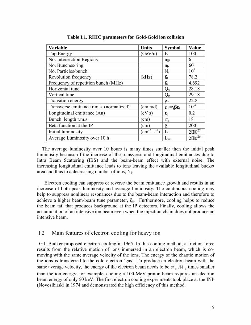
Table I.1. RHIC parameters for Gold-Gold ion collision

Variable Units Symbol ValueTop Energy (GeV/u) E 100No. Intersection Regions nIP 6No. Bunches/ring nb 60No. Particles/bunch Ni 109

Revolution frequency (kHz) f0 78.2Frequency of repetition bunch (MHz) fb 4.692Horizontal tune Qx 28.18Vertical tune Qz 29.18Transition energy γtr 22.8Transverse emittance r.m.s. (normalized) (cm rad) εnt=γβεt 10-4

Longitudinal emittance (Au) (eV s) εl 0.2Bunch length r.m.s. (cm) σs 18Beta function at the IP (cm) βIP 200Initial luminosity (cm-2 s-1) Li 2⋅1027

Average Luminosity over 10 h Lav 2⋅1026

The average luminosity over 10 hours is many times smaller then the initial peakluminosity because of the increase of the transverse and longitudinal emittances due toIntra Beam Scattering (IBS) and the beam-beam effect with external noise. Theincreasing longitudinal emittance leads to ions leaving the available longitudinal bucketarea and thus to a decreasing number of ions, Ni.

Electron cooling can suppress or reverse the beam emittance growth and results in anincrease of both peak luminosity and average luminosity. The continuous cooling mayhelp to suppress nonlinear resonances due to the beam-beam interaction and therefore toachieve a higher beam-beam tune parameter, ξii. Furthermore, cooling helps to reducethe beam tail that produces background at the IP detectors. Finally, cooling allows theaccumulation of an intensive ion beam even when the injection chain does not produce anintensive beam.

I.2 Main features of electron cooling for heavy ion

G.I. Budker proposed electron cooling in 1965. In this cooling method, a friction forceresults from the relative motion of ions immersed in an electron beam, which is co-moving with the same average velocity of the ions. The energy of the chaotic motion ofthe ions is transferred to the cold electron ‘gas’. To produce an electron beam with thesame average velocity, the energy of the electron beam needs to be ie Mm / times smallerthan the ion energy; for example, cooling a 100-MeV proton beam requires an electronbeam energy of only 50 keV. The first electron cooling experiments took place at the INP(Novosibirsk) in 1974 and demonstrated the high efficiency of this method.

6

The first cooling theory estimates used a plasma model of energy exchange in anelectron-ion plasma. When an ion with a charge eZi moves past an electron with velocityV at a distance ρ, the field of the ion, which is Zi e/ρ2, kicks the electron and changes itsmomentum by ∆pe= Zie

2/ρ2 ×2 ρ/V. The ion energy loss is ∆pe2/(2me). Using the small-

displacement (Born's) approximation for electron motion the friction force, integratedover the range of distances, can be written in the form:

)ln(4

221

min

max2

42max

min

22

42

ρρπρπρ

ρ

ρ

ρ Vm

neZd

Vm

neZ

dt

dE

VF

e

ei

e

ei === ∫ , (4)

where ρmax and ρmin are the maximal and minimal impact distances. Let us consider anelectron beam with a density that is not too high. This would be defined as the plasmafrequency being smaller than the inverse time of flight in the cooling section, or

τπω /14 <<= eee rnc . (in the beam’s reference system )/( clcooling γβτ = ). Then the

maximum impact distance is determined by the path of ions in the electron beam,τρ V=max (5)

and the minimal impact distance is determined by the condition that the displacement ofthe electrons during the interaction time τi =ρ/V , where 222 )/( ieii meZV τρτρ ≈= , isgiven by:

22

2

min)/( cV

rZ

Vm

eZ ei

e

i ==ρ . (6)

When the electrons have their own chaotic motion with a velocity distributionee VdVf 3)(

! , the calculation of the friction force requires averaging the friction force overthe distribution:

eee VdVfVVFF ∫ −= 3)()(!!!!!

. (7)

For example, if the distribution )( eVf! corresponds to a uniform sphere in velocity space,

constVf e =)(! for

ce VV <! , then the friction force grows linearly from center of the

electron velocity distribution to the edge, and outside it decreases as V-2. The cooling ratereaches a maximal value which is given for a small ion velocity, contained inside theelectron velocity distribution V <Vc, by:

)ln(4

min

max3

24

max ρρπλ

cie

i

VMm

Ze= (8)

For high ion velocities with V>Vc the cooling decrement drops as V-3 :

)ln(4

min

max3

24

ρρπ

λVMmZe

ie

i= (9)

In the first experiment at NAP-M, a 65-MeV proton beam was cooled by an electronbeam with an energy of 35 keV. The temperature was Ete=0.2 eV, two times higherenergy than the thermal motion of the electrons due to the electron-gun’s cathodetemperature (1000 K, 0.1 eV). The thermal velocity of the electrons with this energy was

7

7103.2 ⋅=eV cm/s. This results in a cooling time of 3 s for a velocity, given at beamreference system, of less than 2.3⋅107 cm/s. In the NAP-M experiment it was discovered that the cooling time continued todecrease for a low transverse ions velocity V<Vc , and in fact it turned out to be less than0.1 s instead of 3 s. Such a dramatic increase in cooling efficiency was a result of thecombined effect of two factors: first, the presence of a longitudinal magnetic field in thecooling section, and second, an extremely low spread in the longitudinal electronvelocities after acceleration. The longitudinal magnetic field was used to transport theelectron beam from the cathode to the proton beam cooling section and further down tothe electron beam collector. In the language of electron cooling, the magnetic field``magnetizes" the transverse electrons motion. It means that the ions interact with ‘cool’electrons, having a Larmor circle with a relatively small radius, ρL=mVc/eB, where B isthe magnetic field (for NAP ρL=10-3 cm), rather than with hot (and fast) free electrons.This phenomenon resulted in both an enhancement of the cooling rate and cooling of theions to temperatures many times lower than the cathode temperature 1500o K. Thus,NAP-M obtained a proton longitudinal temperature of about 1o K.

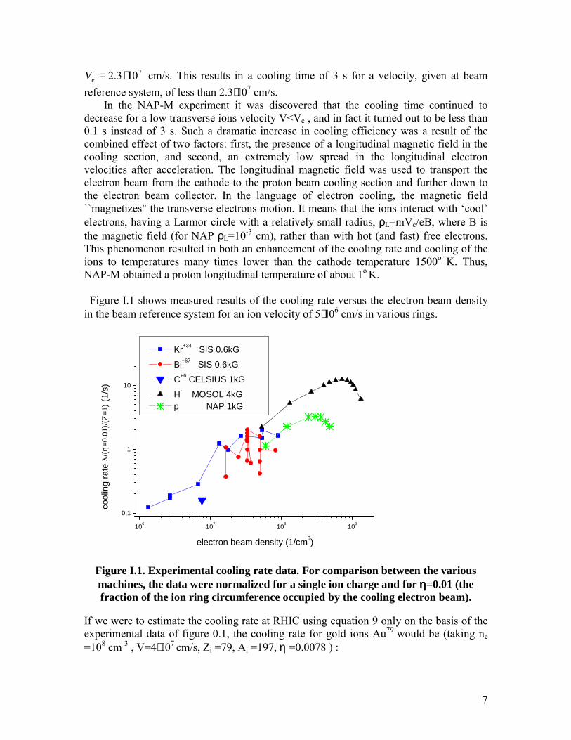
Figure I.1 shows measured results of the cooling rate versus the electron beam densityin the beam reference system for an ion velocity of 5⋅106 cm/s in various rings.

106 107 108 109

0,1

1

10

Kr+34 SIS 0.6kG Bi+67 SIS 0.6kG C+6 CELSIUS 1kG H- MOSOL 4kG p NAP 1kG

cool

ing

rate

λ/(

η=0.

01)/(

Ζ=1)

(1/s

)

electron beam density (1/cm3)

Figure I.1. Experimental cooling rate data. For comparison between the variousmachines, the data were normalized for a single ion charge and for ηηηη=0.01 (thefraction of the ion ring circumference occupied by the cooling electron beam).

If we were to estimate the cooling rate at RHIC using equation 9 only on the basis of theexperimental data of figure 0.1, the cooling rate for gold ions Au79 would be (taking ne=108 cm-3 , V=4⋅107 cm/s, Zi =79, Ai =197, η =0.0078 ) :

8

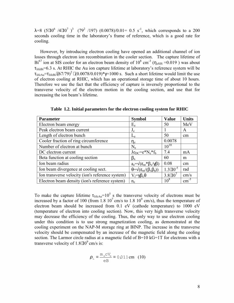
λ=8 (5⋅106 /4⋅107 )3 (792 /197) (0.0078)/0.01= 0.5 s-1, which corresponds to a 200seconds cooling time in the laboratory’s frame of reference, which is a good rate forcooling.

However, by introducing electron cooling have opened an additional channel of ionlosses through electron ion recombination in the cooler section. The capture lifetime ofBi67 ion at SIS cooler for an electron beam density of 108 cm-3 (ηeSIS =0.019 ) was aboutτlifeBi=6.3 s. At RHIC the Au ion capture lifetime at laboratory’s reference system will beτlifeAu=τlifeBi⋅(67/79)2 ⋅ (0.0078/0.019)*γ=1000 s. Such a short lifetime would limit the useof electron cooling at RHIC, which has an operational storage time of about 10 hours.Therefore we use the fact that the efficiency of capture is inversely proportional to thetransverse velocity of the electron motion in the cooling section, and use that forincreasing the ion beam’s lifetime.

Table I.2. Initial parameters for the electron cooling system for RHIC

Parameter Symbol Value UnitsElectron beam energy Ee 50 MeVPeak electron beam current Je 1 ALength of electron bunch Le 50 cmCooler fraction of ring circumference ηe 0.0078Number of electron at bunch Ne 1010

DC electron current JeDC=e*Ne*fb 7.4 mABeta function at cooling section βx 60 mIon beam radius ae=√(εnt*βx/γβ) 0.08 cmIon beam divergence at cooling sect. θ=√(εnt/(βxβγ)) 1.3⋅10-5 radIon transverse velocity (ion's reference system) Vi=γβcθ 3.8⋅107 cm/sElectron beam density (ion's reference system) ne 108 cm-3

To make the capture lifetime τlifeAu=105 s the transverse velocity of electrons must beincreased by a factor of 100 (from 1.8 107 cm/s to 1.8 109 cm/s), thus the temperature ofelectron beam should be increased from 0.1 eV (cathode temperature) to 1000 eV(temperature of electron into cooling section). Now, this very high transverse velocitymay decrease the efficiency of the cooling. Thus, the only way to use electron coolingunder this condition is to use strong magnetization cooling, as demonstrated at thecooling experiment on the NAP-M storage ring at BINP. The increase in the transversevelocity should be compensated by an increase of the magnetic field along the coolingsection. The Larmor circle radius at a magnetic field of B=10 kG=1T for electrons with atransverse velocity of 1.8⋅109 cm/s is:

011.0==eB

cVm eeLρ cm (10)

9

Since this Larmor radius is several times smaller than the radius of both beams, ae=0.07cm, that gives hope to not losing too much cooling rate. What the cooling time which isreally needed for the suppression of IBS, beam-beam interaction and other sources ofnoise is will remain an open question up to a real cooling experiment. The cooling timeof 200 s looks very powerful, and it is hard to believe that fast heating effects exist atRHIC such that can increase the beam emittance in 200 s.

10

1 MAIN SCENARIO FOR ELECTRONCOOLINGIn this section we cover the subjects of continuous cooling at the collider's storage state,at beam injection energy and the usage of cooling for accumulation of beam.

1.1. Continuous cooling at the collider’s storage energy

This report provides a preliminary study of the beneficial effect of electron cooling onRHIC luminosity for gold - gold collisions. Various parameters are not optimized at thispoint; therefore we can expect changes as the work progresses. We will show how thebeneficial effect of electron cooling changes when we vary RHIC parameters for a gold-ion beam. Electron cooling will help to optimize RHIC’s parameters for variousexperiments. For some experiments it may be necessary to have a maximal integralluminosity over the storage period, but other experiments may require, for example, aconstant luminosity over the storage period.The basic sets of the parameters used in the Cooling Scenario for the RHIC gold-ionbeam are listed in the table below:

Table 1.1. GOLD nominal beam parameters at various stages

The following results are taken from a simulation program. We will compare variousbeam parameters as a function of time at RHIC storage (top) energy, without cooling andwith cooling with various electron currents. A single particle Mathcad code is used forthe simulation of cooling. The advantage of this code is a very fast response, thedisadvantage - large fluctuation near equilibrium. This version is useful for fast testing ofof the influence of various parameters

The simulation of beam heating (increase in transverse and longitudinal ion beamemittances and the associated losses of ions) is based on the simplest IBS model using arandom oscillation of the colliding ion beam at the interaction point with an amplitude of0.1 microns. Ions are lost by escaping the longitudinal bucket area, by dissociation atInteraction Points and pair production with a cross section of 212 barns, and by capture ofelectrons at the electron cooler.

In the simulation the fraction η of ions held in the bunch is taken as the ratio of the bucketarea to the emittance, η=2*εlon0/(εlon+εlon0), or as 1 when all the ions are contained in thebucket. When cooling is applied and the longitudinal emittance is decreasing, εlon<εlon0

Units Injection Store start Store endNominal beam int. Ni 109 1.0 1.0Transverse emittance εni 95% π*µm, normalized 10 15 40RMS bunch length σs m 0.47 0.12 0.2RMS momentum spread 0.001 0.27 0.53 0.9

11

this coefficient equals 1. With the same parameters it is possible to see an increase in thenumber of ions as a result of capture of coasting ions into the RF bucket. Ions may escapethe bucket at some particular time. When the ions escape the bucket they are notimmediately lost, but they do not take part in luminosity production. Electron coolingmay return some part of these ions to the RF bucket. More information about theelectron beam parameters is embedded in the Mathcad rep4a1a.mcd file.

The performance of RHIC under cooling. Given the mechanisms IBS, electroncooling, beam dissociation and recombination, we can now calculate the performance ofRHIC at storage energy with a particular electron cooling current. We take the followingparameters for electron cooling:

Table 1.2. List of basic parameters list used for the simulation of electron cooling inthis section

Number of electron in a single cooling bunch Ne= 0---1011

Electron bunch length r.m.s. [cm] σs =20Frequency of repetition ion bunches [MHz] fb=4.6Average electron current [mA] Iav=0---74Peak electron current [A] Ipeak= 0--- 9.6Magnet field at cooling section [kG] B=10Transverse electron temperature in beam’s reference system [eV] T⊥ =1000Electron beam diameter [mm] a=2

The results of the simulations are summarized in Figure 1.1.1. The luminosity at a singleInteraction Point is defined as:

bIPni

i fNLβπε

γβ4

2

= , (1)

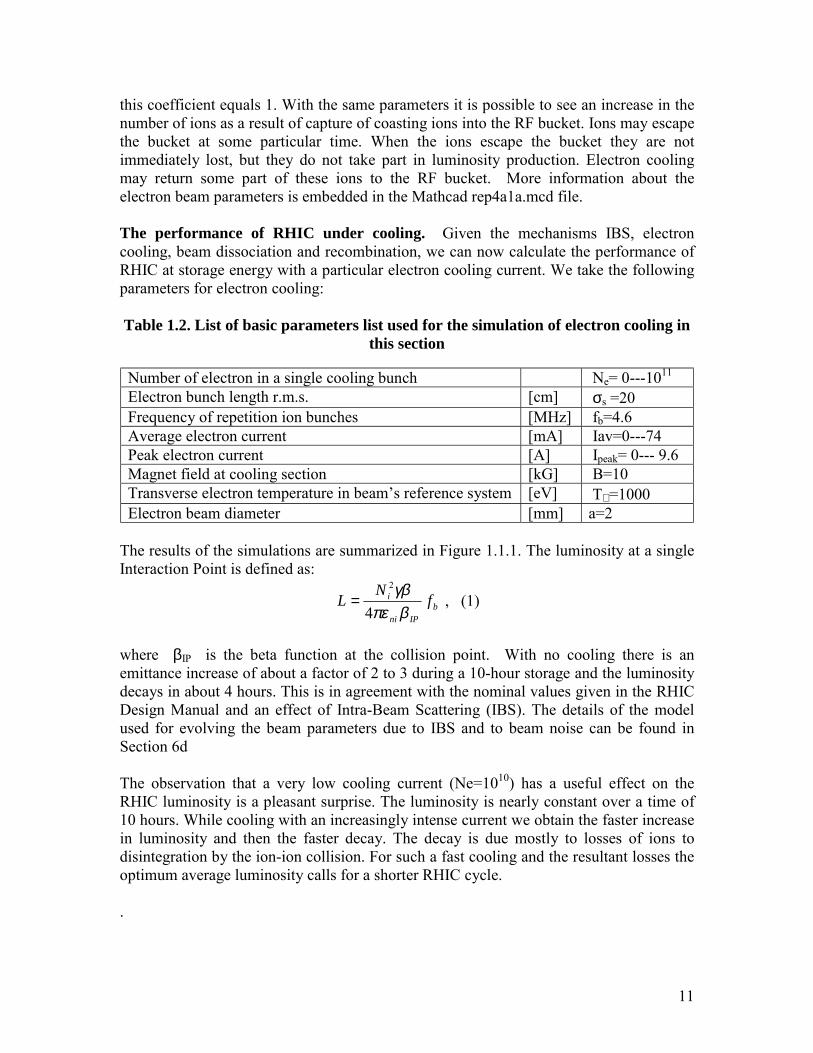
where βIP is the beta function at the collision point. With no cooling there is anemittance increase of about a factor of 2 to 3 during a 10-hour storage and the luminositydecays in about 4 hours. This is in agreement with the nominal values given in the RHICDesign Manual and an effect of Intra-Beam Scattering (IBS). The details of the modelused for evolving the beam parameters due to IBS and to beam noise can be found inSection 6d

The observation that a very low cooling current (Ne=1010) has a useful effect on theRHIC luminosity is a pleasant surprise. The luminosity is nearly constant over a time of10 hours. While cooling with an increasingly intense current we obtain the faster increasein luminosity and then the faster decay. The decay is due mostly to losses of ions todisintegration by the ion-ion collision. For such a fast cooling and the resultant losses theoptimum average luminosity calls for a shorter RHIC cycle.

.

12

0 2 4 6 8 10

1E26

1E27

1E28

no cooling electron cooling Ne=1010

electron cooling Ne=3 1010


Lum

inos

ity (c

m-2s-1

)

time (h)

Figure 1.1. The luminosity at a single IP versus time for different cooling current.

0 2 4 6 8 10

1E-5

1E-4

1E-3

no cooling cooling Ne=1010

cooling Ne=3 1010

cooling Ne=1011

emitt

ance

(r.m

.s.)

(mm

*mra

d π )

time (h)

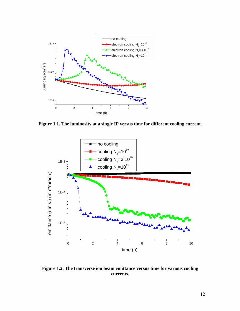
Figure 1.2. The transverse ion beam emittance versus time for various coolingcurrents.

13

Figure 1.2 shows the contribution of the transverse beam emittance to the development ofthe luminosity show in Figure 1.1. An equilibrium between the IBS and coolingprocesses takes place at an ion beam emittance of εnieq=0.3-0.1 mm*mrad. The largeinitial the ion beam emittance of RHIC, 4 mm*mrad leads to a delay of the cooling take-off. A preliminary cooling at injection energy would help to avoid this delay and to startfrom the higher luminosity. If this were the case, the top energy electron cooling, used forobtaining an IBS–cooling equilibrium, would require a lower electron current.

0 2 4 6 8 100

20

40

no cooling electron cooling Ne=1010



bunc

h le

ngth

(cm

)

time (h)

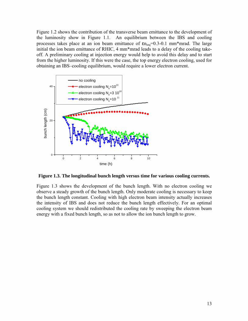
Figure 1.3. The longitudinal bunch length versus time for various cooling currents.

Figure 1.3 shows the development of the bunch length. With no electron cooling weobserve a steady growth of the bunch length. Only moderate cooling is necessary to keepthe bunch length constant. Cooling with high electron beam intensity actually increasesthe intensity of IBS and does not reduce the bunch length effectively. For an optimalcooling system we should redistributed the cooling rate by sweeping the electron beamenergy with a fixed bunch length, so as not to allow the ion bunch length to grow.

14

0 2 4 6 8 10

1E8

1E9


cooling Ne=3 1010

cooling Ne=1011

Num

ber o

f ion

s at

bun

ch

time (h)

Figure 1.4. The number of ions in a single bunch versus time for various coolingcurrents.

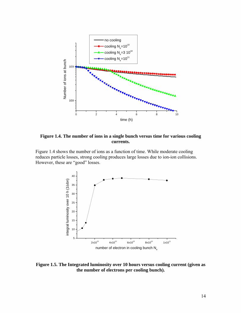
Figure 1.4 shows the number of ions as a function of time. While moderate coolingreduces particle losses, strong cooling produces large losses due to ion-ion collisions.However, these are “good” losses.

2x1010 4x1010 6x1010 8x1010 1x1011

5

10

15

20

25

30

35

40

inte

gral

lum

inos

ity o

ver 1

0 h

(1/µ

bn)

number of electron in cooling bunch Ne

Figure 1.5. The Integrated luminosity over 10 hours versus cooling current (given asthe number of electrons per cooling bunch).

15

Figure 1.5 shows that after reaching an electron bunch intensity Ne=2 1010 the moreintensive cooling does not benefit the integrated luminosity over a 10 hours run period.The disintegration cross section σtot=212 nb limits the integrated luminosity through:

( )totIP

bi

n

nNLdt

σ=∫ max

, (2)

where nb=60 is the number of bunches in the storage ring, and nIP=6 is the number ofinteraction points delivering this luminosity. From equation 2 we can see that themaximal integrated luminosity (over time ∞−0 ) equals 47 1/µbn. An integratedluminosity of 38 1/µbn on figure 1.5 means that 80% of the ions were disintegrated in IPcollisions.

The parameter that measures the intensity of the interaction in the IP through the spacecharge of the ion bunches is the tune shift parameter at a single interaction point:

ni

iiii

rNπε

ξ4

= . (3)

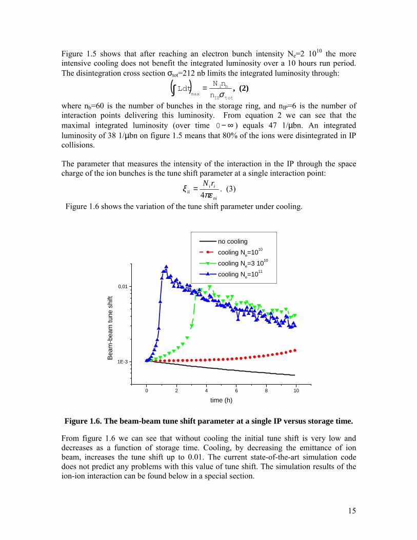
Figure 1.6 shows the variation of the tune shift parameter under cooling.

0 2 4 6 8 10

1E-3

0,01


cooling Ne=3 1010

cooling Ne=1011

Beam

-bea

m tu

ne s

hift

time (h)

Figure 1.6. The beam-beam tune shift parameter at a single IP versus storage time.

From figure 1.6 we can see that without cooling the initial tune shift is very low anddecreases as a function of storage time. Cooling, by decreasing the emittance of ionbeam, increases the tune shift up to 0.01. The current state-of-the-art simulation codedoes not predict any problems with this value of tune shift. The simulation results of theion-ion interaction can be found below in a special section.

16

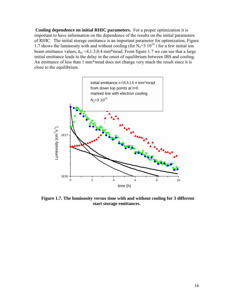
Cooling dependence on initial RHIC parameters. For a proper optimization it isimportant to have information on the dependence of the results on the initial parametersof RHIC. The initial storage emittance is an important parameter for optimization. Figure1.7 shows the luminosity with and without cooling (for Ne=3 1010 ) for a few initial ionbeam emittance values, εni =4,1.3,0.4 mm*mrad. From figure 1.7 we can see that a largeinitial emittance leads to the delay in the onset of equilibrium between IBS and cooling.An emittance of less than 1 mm*mrad does not change very much the result since it isclose to the equilibrium.

0 2 4 6 8 101E26

1E27

initial emittance ε=15,5,1.5 π mm*mradfrom down top points at t=0marked line with electron cooling

Ne=3 1010

Lum

inos

ity (c

m-2s-1

)

time (h)

Figure 1.7. The luminosity versus time with and without cooling for 3 differentstart storage emittances.

17

0 2 4 6 8 10

1E25

1E26

1E27

black line no cooling Ni=109, Ne=0

red line cooling Ni= 109, Ne=3 1010

black dashed no cooling Ni=108, Ne=0

red dashed cooling Ne= 3 108, Ne=3 1010

Lum

inos

ity (c

m-2 s

-1)

time (h)

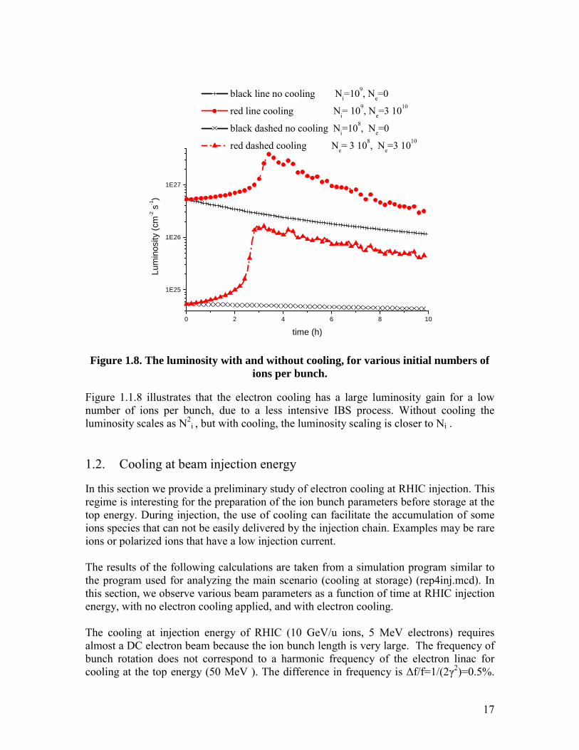
Figure 1.8. The luminosity with and without cooling, for various initial numbers ofions per bunch.

Figure 1.1.8 illustrates that the electron cooling has a large luminosity gain for a lownumber of ions per bunch, due to a less intensive IBS process. Without cooling theluminosity scales as N2

i , but with cooling, the luminosity scaling is closer to Ni .

1.2. Cooling at beam injection energy

In this section we provide a preliminary study of electron cooling at RHIC injection. Thisregime is interesting for the preparation of the ion bunch parameters before storage at thetop energy. During injection, the use of cooling can facilitate the accumulation of someions species that can not be easily delivered by the injection chain. Examples may be rareions or polarized ions that have a low injection current.

The results of the following calculations are taken from a simulation program similar tothe program used for analyzing the main scenario (cooling at storage) (rep4inj.mcd). Inthis section, we observe various beam parameters as a function of time at RHIC injectionenergy, with no electron cooling applied, and with electron cooling.

The cooling at injection energy of RHIC (10 GeV/u ions, 5 MeV electrons) requiresalmost a DC electron beam because the ion bunch length is very large. The frequency ofbunch rotation does not correspond to a harmonic frequency of the electron linac forcooling at the top energy (50 MeV ). The difference in frequency is Δf/f=1/(2γ2)=0.5%.

18

The simplest solution to the problem of bunch synchronization is to use a separateaccelerator system adapted to cooling at injection energy. The cooling calculation usedthe following parameters:

Table 1.3. Parameters for cooling calculation

Electron bunch length 1.1-m r.m.s.Ion bunch length 1.1-m r.m.s.Number of Ion bunches 60Average electron cooling current 15 mAPeak electron cooling current 0.3 A

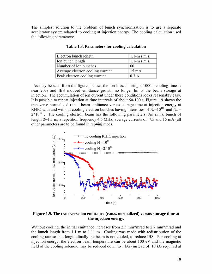
As may be seen from the figures below, the ion losses during a 1000 s cooling time isnear 20% and IBS induced emittance growth no longer limits the beam storage atinjection. The accumulation of ion current under these conditions looks reasonably easy.It is possible to repeat injection at time intervals of about 50-100 s. Figure 1.9 shows thetransverse normalized r.m.s. beam emittance versus storage time at injection energy atRHIC with and without cooling electron bunches having intensities of Ne=1010 and Ne =2*1010 . The cooling electron beam has the following parameters: An r.m.s. bunch oflength σ=1.1 m, a repetition frequency 4.6 MHz, average currents of 7.5 and 15 mA (allother parameters are to be found in rep4inj.mcd).

0 200 400 600 800 1000

1E-5

1E-4

1E-3 no cooling RHIC injection cooling Ne=1010

cooling Ne=2 1010

ion

beam

nor

m. r

.m.s

. em

ittan

ce (c

m*r

ad)

time (s)

Figure 1.9. The transverse ion emittance (r.m.s. normalized) versus storage time atthe injection energy.

Without cooling, the initial emittance increases from 2.5 mm*mrad to 2.7 mm*mrad andthe bunch length from 1.1 m to 1.11 m . Cooling was made with redistribution of thecooling rate so that longitudinally the beam is not cooled, to reduce IBS. For cooling atinjection energy, the electron beam temperature can be about 100 eV and the magneticfield of the cooling solenoid may be reduced down to 1 kG (instead of 10 kG required at

19

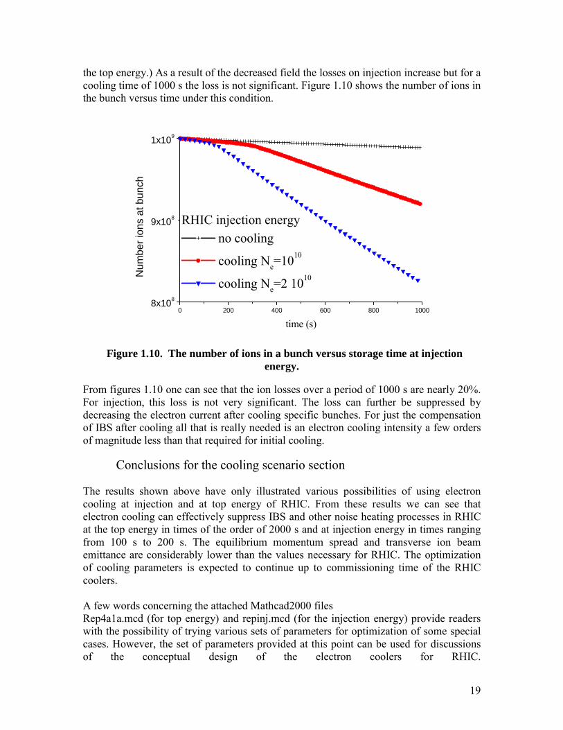
the top energy.) As a result of the decreased field the losses on injection increase but for acooling time of 1000 s the loss is not significant. Figure 1.10 shows the number of ions inthe bunch versus time under this condition.

0 200 400 600 800 10008x108

9x108

1x109

RHIC injection energy no cooling

cooling Ne=1010

cooling Ne=2 1010Num

ber i

ons

at b

unch

time (s)

Figure 1.10. The number of ions in a bunch versus storage time at injectionenergy.

From figures 1.10 one can see that the ion losses over a period of 1000 s are nearly 20%.For injection, this loss is not very significant. The loss can further be suppressed bydecreasing the electron current after cooling specific bunches. For just the compensationof IBS after cooling all that is really needed is an electron cooling intensity a few ordersof magnitude less than that required for initial cooling.

Conclusions for the cooling scenario section

The results shown above have only illustrated various possibilities of using electroncooling at injection and at top energy of RHIC. From these results we can see thatelectron cooling can effectively suppress IBS and other noise heating processes in RHICat the top energy in times of the order of 2000 s and at injection energy in times rangingfrom 100 s to 200 s. The equilibrium momentum spread and transverse ion beamemittance are considerably lower than the values necessary for RHIC. The optimizationof cooling parameters is expected to continue up to commissioning time of the RHICcoolers.

A few words concerning the attached Mathcad2000 filesRep4a1a.mcd (for top energy) and repinj.mcd (for the injection energy) provide readerswith the possibility of trying various sets of parameters for optimization of some specialcases. However, the set of parameters provided at this point can be used for discussionsof the conceptual design of the electron coolers for RHIC.

20

2. LUMINOSITY UNDER COOLING

2.1 Beam Parameters at the Interaction Points

At RHIC, collisions take place at nIP=6 Interaction Points. For simplifying thediscussions below, we will assume equivalency of all the IPs, with parameters listed inthe table 2.1:

Table 2.1 RHIC parameters used in various calculations

Parameter Symbol Value UnitsBeta function at IP β IP 2 m Crossing angle 0 RadiansNumber of ions per bunch Ni 109

Number of bunches in the ring nb 60Initial ion r.m.s. normalized emittance εni 3.7 mm⋅mradInitial r.m.s. bunch length σs 22 cmInitial momentum spread σp 1.46⋅10-3

2.2. Beam-beam interaction

The main beam-beam parameter for the interaction is the linear tune shift at the IP:

i

iiii

n

rN

πεξ

4= (1)

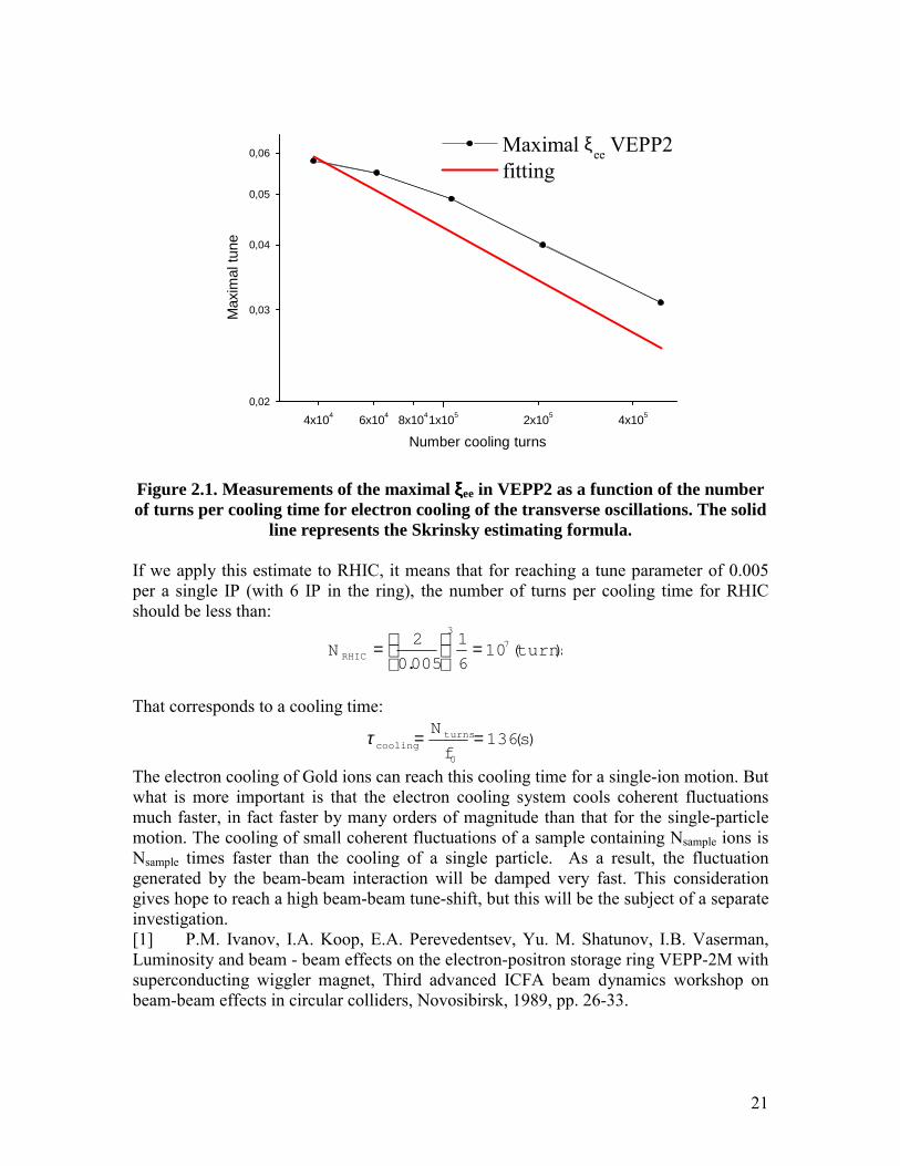
This parameter is a measure of the strength of nonlinear resonances which cause adiffusion of ions to large amplitude oscillations. The beam-beam parameter for RHICstorage at top energy is ξii=3.8⋅10-3. The result of a simulation made at BINP shows thatthe power of these resonances for the proper ring lattice becomes significant if ξii>0.05.Any low-power cooling is useful for preventing the blowup of the beam during collisionsof ion bunches for a small tune-shift. Experience with electron-positron colliders showsthat increased cooling helps to reach a higher tune shift and luminosity. The Figure 2.1shows measurement results of the maximal tune shift in the collider VEPP2M at anenergy range 300-700 MeV [1] when the syhrotron radiation cooling changessignificantly by changing the radiated power.The maximal beam-beam tune-shift as a function of the number of turns in one coolingtime may be estimated by a simple power fitting approximation (Skrinsky formula):

3/1max

2

cooling

ii N=ξ . (2)

The solid line in the figure shows calculation according this line.

21

4x104 6x104 8x1041x105 2x105 4x1050,02

0,03

0,04

0,05

0,06 Maximal ξee VEPP2

fitting

Max

imal

tune

Number cooling turns

Figure 2.1. Measurements of the maximal ξξξξee in VEPP2 as a function of the numberof turns per cooling time for electron cooling of the transverse oscillations. The solid

line represents the Skrinsky estimating formula.

If we apply this estimate to RHIC, it means that for reaching a tune parameter of 0.005per a single IP (with 6 IP in the ring), the number of turns per cooling time for RHICshould be less than:

)(106

1

005.0

2 7

3

turnsN RHIC =

=

That corresponds to a cooling time:

)(1360

sf

N turnscooling ==τ

The electron cooling of Gold ions can reach this cooling time for a single-ion motion. Butwhat is more important is that the electron cooling system cools coherent fluctuationsmuch faster, in fact faster by many orders of magnitude than that for the single-particlemotion. The cooling of small coherent fluctuations of a sample containing Nsample ions isNsample times faster than the cooling of a single particle. As a result, the fluctuationgenerated by the beam-beam interaction will be damped very fast. This considerationgives hope to reach a high beam-beam tune-shift, but this will be the subject of a separateinvestigation.[1] P.M. Ivanov, I.A. Koop, E.A. Perevedentsev, Yu. M. Shatunov, I.B. Vaserman,Luminosity and beam - beam effects on the electron-positron storage ring VEPP-2M withsuperconducting wiggler magnet, Third advanced ICFA beam dynamics workshop onbeam-beam effects in circular colliders, Novosibirsk, 1989, pp. 26-33.

22

2.3 Noise and beam-beam Diverse sources of noise produce random fluctuations of the orbit position at theInteraction Point. Kicker magnets, electrostatic plates, or high frequency vibrations ofquadrupole magnets or the vacuum chamber can produce these noises. As a result, the ionbunch receives a random kick at the IP, with an amplitude proportional to the deflectionof the counter rotating bunch from the central position x:

IP

ii

xx

βπξθ 2)( =∆ (3)

This kick produces coherent oscillations of the ion bunch, which persist over thedecoherence-time of RHIC. This energy is transferred to the chaotic thermal motion ofions. However, with electron cooling, the energy of this decaying coherent oscillation isdamped by a coherent interaction with the cooling electron beam. If we neglect coherentdamping, the heating rate of the beam emittance by this process is equal to:

22

0

)2(xnf

dt

d

IP

iiIP

i

βπξε = (4)

As the process of cooling proceeds, the density of the ion beam increases and ξii increasesuntil such a time that an equilibrium state is reached, when the cooling is equal to thisheating source. The simulation code rep4a1a.mcd takes this process into account.

The decay time of the coherent oscillation after a single kick can be estimated as follows[1]. A tune spread is generated equal to:

IPiinQ ξ2.0≈∆ (5)and this leads to a damping of the coherent oscillation in a number of turns given by

)(10001

turnsQ

N decoh ≈∆

= (6)

The requirement to the coherent cooling rate comes from this number of turns necessaryto damp the coherent oscillation.

[1] V. Lebedev, V. Parkhomchuk, V. Shiltsev, G. Stupakov, Emittance growth due tonoise and its suppression with feedback system in large hadron colliders, ParticleAccelerators, V44, pp.147-264,(1994)

2.4 Simulation of beam-beam effects for the gold ion collisions at RHIC.

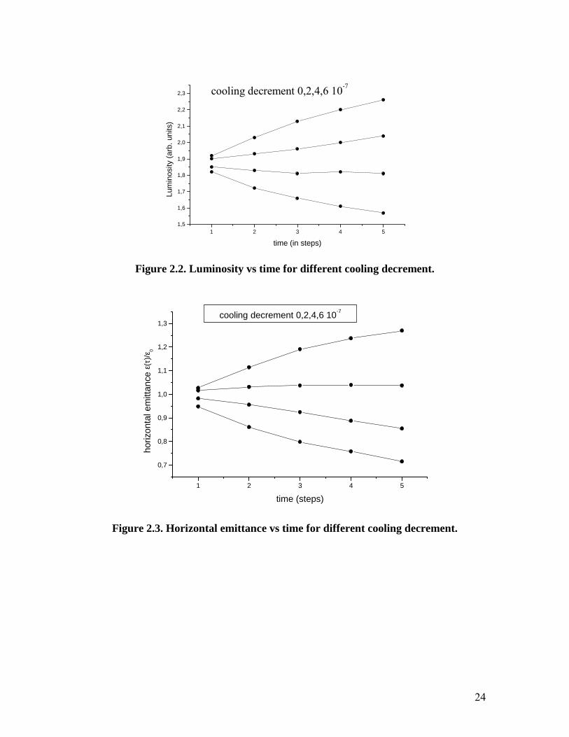
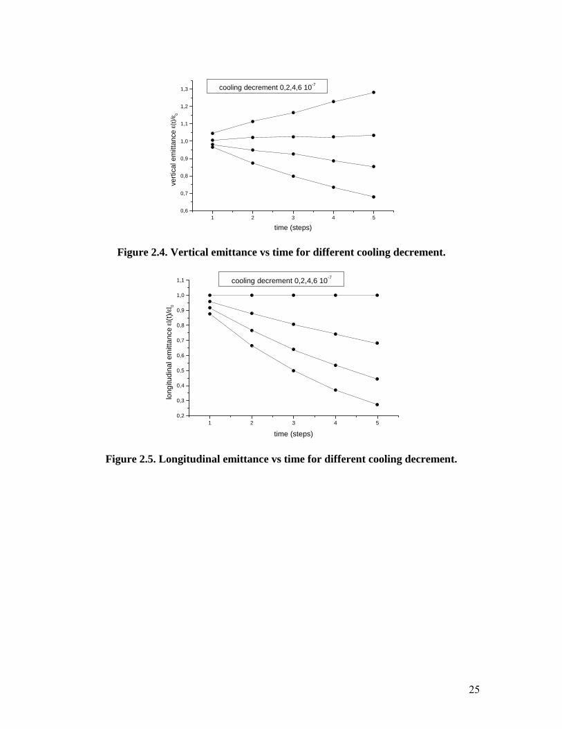
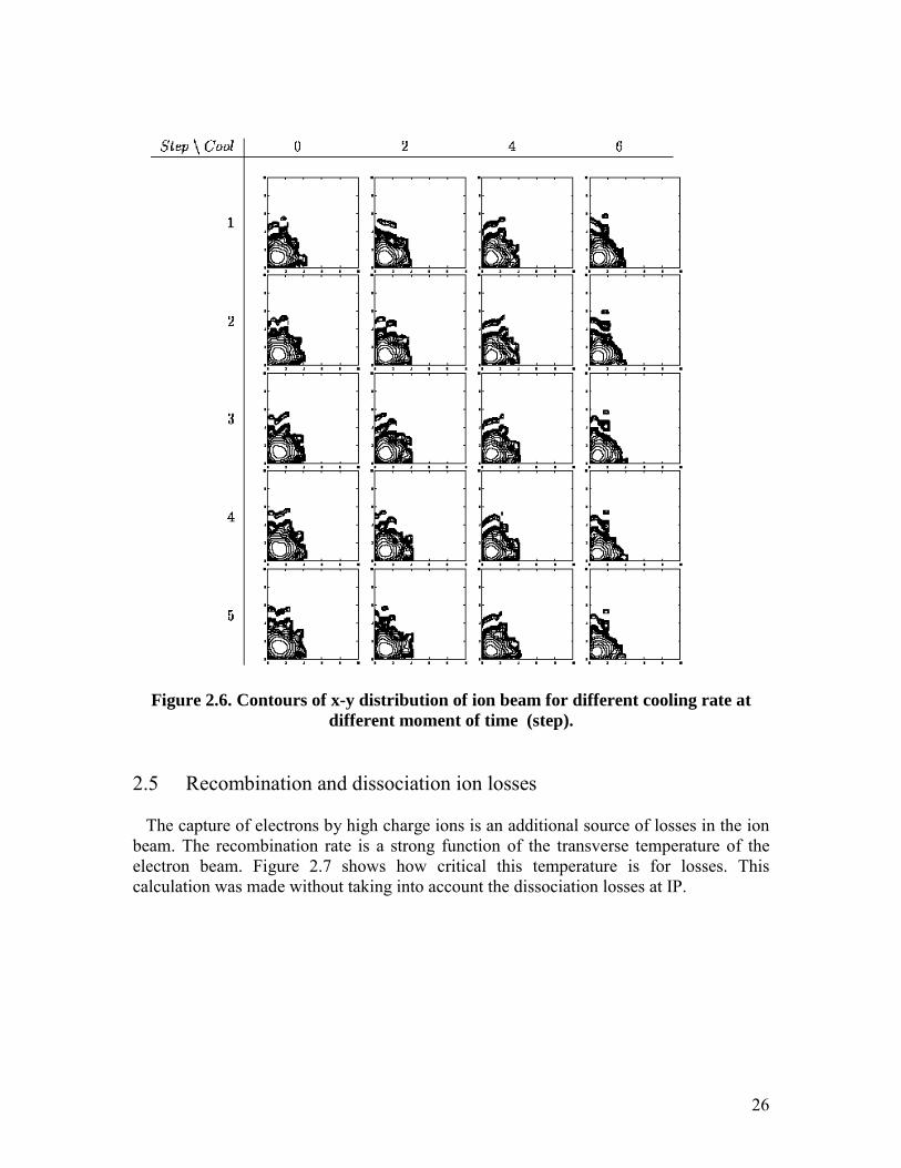
We used a ‘weak-strong’ model, where the ‘strong’ bunch has the initial conditionsduring all the simulation time, and the ‘weak’ one is represented by 1000 macroparticles,which are tracked independently. The other simulation parameters are listed below:• The betatron tunes are: Qx=28.18, Qy=29.18, synchrotron tune is Qs=0.006. 6–fold

symmetry of the ring. Simple linear transport map between the Interaction Points: tuneadvances are 4.6967, 4.8633, 0.001, respectively. No radiation damping and noiseswere accounted.

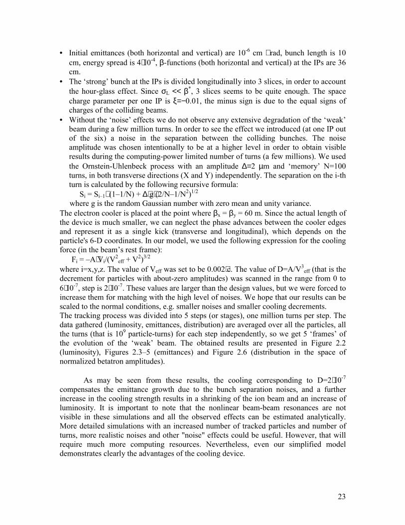
23

• Initial emittances (both horizontal and vertical) are 10-6 cm ⋅ rad, bunch length is 10cm, energy spread is 4⋅10-4, β-functions (both horizontal and vertical) at the IPs are 36cm.

• The ‘strong’ bunch at the IPs is divided longitudinally into 3 slices, in order to accountthe hour-glass effect. Since σL << β*, 3 slices seems to be quite enough. The spacecharge parameter per one IP is ξ=−0.01, the minus sign is due to the equal signs ofcharges of the colliding beams.

• Without the ‘noise’ effects we do not observe any extensive degradation of the ‘weak’beam during a few million turns. In order to see the effect we introduced (at one IP outof the six) a noise in the separation between the colliding bunches. The noiseamplitude was chosen intentionally to be at a higher level in order to obtain visibleresults during the computing-power limited number of turns (a few millions). We usedthe Ornstein-Uhlenbeck process with an amplitude ∆=2 µm and ‘memory’ N=100turns, in both transverse directions (X and Y) independently. The separation on the i-thturn is calculated by the following recursive formula:

Si = Si–1⋅ (1–1/N) + ∆⋅g⋅(2/N–1/N2)1/2

where g is the random Gaussian number with zero mean and unity variance.The electron cooler is placed at the point where βx = βy = 60 m. Since the actual length ofthe device is much smaller, we can neglect the phase advances between the cooler edgesand represent it as a single kick (transverse and longitudinal), which depends on theparticle's 6-D coordinates. In our model, we used the following expression for the coolingforce (in the beam’s rest frame): Fi = –A⋅Vi/(V2

eff + V2)3/2

where i=x,y,z. The value of Veff was set to be 0.002⋅c. The value of D=A/V3eff (that is the

decrement for particles with about-zero amplitudes) was scanned in the range from 0 to6⋅10-7, step is 2⋅10-7. These values are larger than the design values, but we were forced toincrease them for matching with the high level of noises. We hope that our results can bescaled to the normal conditions, e.g. smaller noises and smaller cooling decrements.The tracking process was divided into 5 steps (or stages), one million turns per step. Thedata gathered (luminosity, emittances, distribution) are averaged over all the particles, allthe turns (that is 109 particle-turns) for each step independently, so we get 5 ‘frames’ ofthe evolution of the ‘weak’ beam. The obtained results are presented in Figure 2.2(luminosity), Figures 2.3–5 (emittances) and Figure 2.6 (distribution in the space ofnormalized betatron amplitudes).

As may be seen from these results, the cooling corresponding to D=2⋅10-7

compensates the emittance growth due to the bunch separation noises, and a furtherincrease in the cooling strength results in a shrinking of the ion beam and an increase ofluminosity. It is important to note that the nonlinear beam-beam resonances are notvisible in these simulations and all the observed effects can be estimated analytically.More detailed simulations with an increased number of tracked particles and number ofturns, more realistic noises and other "noise" effects could be useful. However, that willrequire much more computing resources. Nevertheless, even our simplified modeldemonstrates clearly the advantages of the cooling device.

24

1 2 3 4 51,5

1,6

1,7

1,8

1,9

2,0

2,1

2,2

2,3 cooling decrement 0,2,4,6 10-7

Lum

inos

ity (a

rb. u

nits

)

time (in steps)

Figure 2.2. Luminosity vs time for different cooling decrement.

1 2 3 4 5

0,7

0,8

0,9

1,0

1,1

1,2

1,3cooling decrement 0,2,4,6 10-7

horiz

onta

l em

ittan

ce ε(

τ)/ε

0

time (steps)

Figure 2.3. Horizontal emittance vs time for different cooling decrement.

25

1 2 3 4 50,6

0,7

0,8

0,9

1,0

1,1

1,2


verti

cal e

mitt

ance

ε(t)/

ε 0

time (steps)

Figure 2.4. Vertical emittance vs time for different cooling decrement.

1 2 3 4 50,2

0,3

0,4

0,5

0,6

0,7

0,8

0,9

1,0


long

itudi

nal e

mitt

ance

ε l(t)

/ε l0

time (steps)

Figure 2.5. Longitudinal emittance vs time for different cooling decrement.

26

Figure 2.6. Contours of x-y distribution of ion beam for different cooling rate atdifferent moment of time (step).

2.5 Recombination and dissociation ion losses

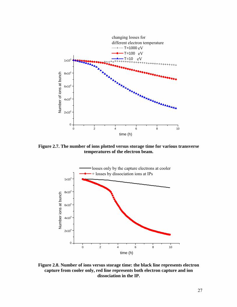
The capture of electrons by high charge ions is an additional source of losses in the ionbeam. The recombination rate is a strong function of the transverse temperature of theelectron beam. Figure 2.7 shows how critical this temperature is for losses. Thiscalculation was made without taking into account the dissociation losses at IP.

27

0 2 4 6 8 100

2x108

4x108

6x108

8x108

1x109

changing losses for different electron temperature

Τ=1000 eV Τ=100 eV Τ=10 eV

Num

ber o

f ion

s at

bun

ch

time (h)

Figure 2.7. The number of ions plotted versus storage time for various transversetemperatures of the electron beam.

0 2 4 6 8 100

2x108

4x108

6x108

8x108

1x109

losses only by the capture electrons at cooler + losses by dissociation ions at IPs

Num

ber i

ons

at b

unch

time (h)

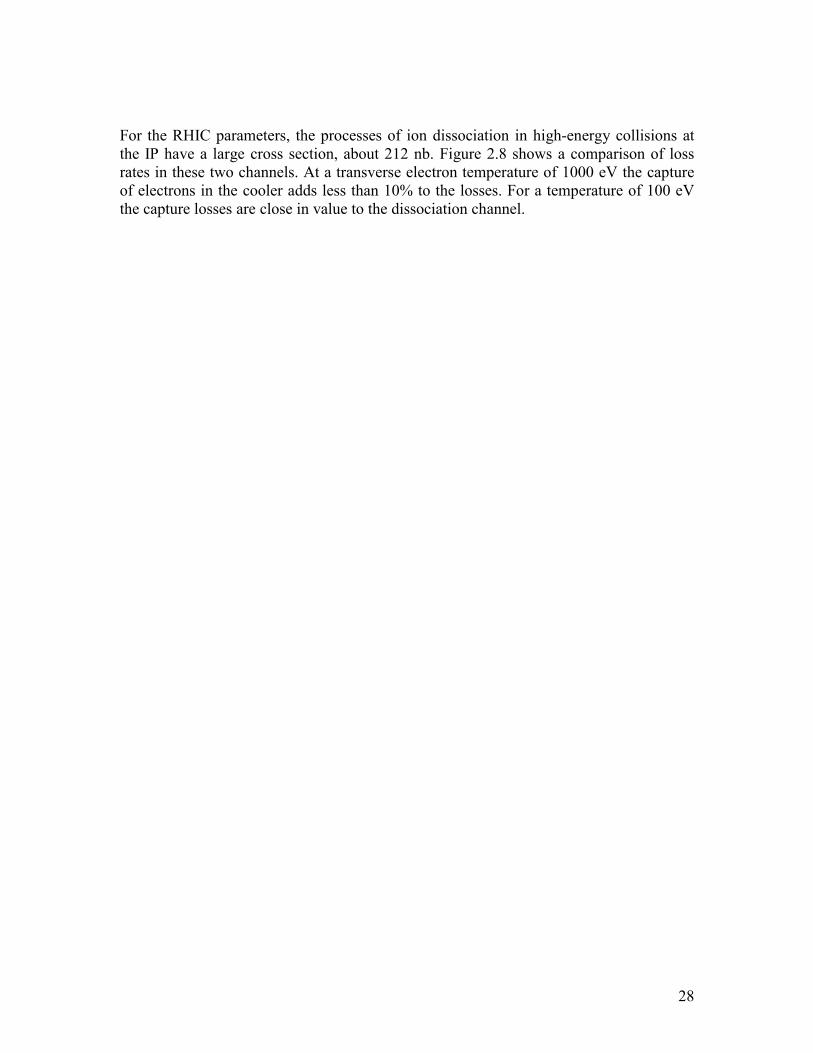
Figure 2.8. Number of ions versus storage time: the black line represents electroncapture from cooler only, red line represents both electron capture and ion

dissociation in the IP.

28

For the RHIC parameters, the processes of ion dissociation in high-energy collisions atthe IP have a large cross section, about 212 nb. Figure 2.8 shows a comparison of lossrates in these two channels. At a transverse electron temperature of 1000 eV the captureof electrons in the cooler adds less than 10% to the losses. For a temperature of 100 eVthe capture losses are close in value to the dissociation channel.

29

3. THE TECHNICAL APPROACH FOR THEELECTRON COOLING SYSTEM3.1 The parameters of the cooling electron beam

3.1.1 Cooling section lengthThere are a few reasons why the cooling section for RHIC should have a large length:

a. The magnetization cooling requires a long interaction time in the beam’sreference frame.

The interaction time τ should satisfy ωLτ >>1 (where ωL=eB/mec is the Larmorfrequency of the electron’s motion in the magnetic field B), and ρmax=Vτ>>ρL=meV⊥ c/(eB), where ρL is the Larmor radius and τ =lcool/(γβc) is the time of flightthrough the cooling section of length lcool.

b. A longer cooling length allows using a smaller electron beam current. A highelectron current for cooling complicates the injection chain and increases the costof the equipment.

c. The cooling time is proportional to the ion's transverse velocity to the third powerand inversely proportional to the density of electron beam. A larger value of theion's beta function in the cooling section decreases the transverse ions velocity.Thus, an increase in βcool leads to a decrease in cooling time as βcool -1/2.

d. The damping decrement of coherent ion beam fluctuations is proportional to τ4. Ifthe cooling parameter is far from being dangerously large, it is advantageous tohave faster coherent cooling by increasing the length of the cooling section.

The long straight sections near the RHIC interaction points permits to have a coolingsolenoid length of about lcool=30 m, a value that will be adopted in this report.

The magnetic field necessary for obtaining a long beam lifetime due to radiative electroncapture is estimated in the introduction as 1 Tesla. Figure 3.1 shows that a magnetic field1 kG over a store time of 10 h is not enough for cooling the ion beam, but with amagnetic field of 10 kG the luminosity is increased significantly after few hours cooling.The difference between 10 kG and 5 kG is not too large. In any case, the solenoid of thecooling section should be superconducting (due to the length and high magnetic field),thus we might as well use a field of 10 kG.

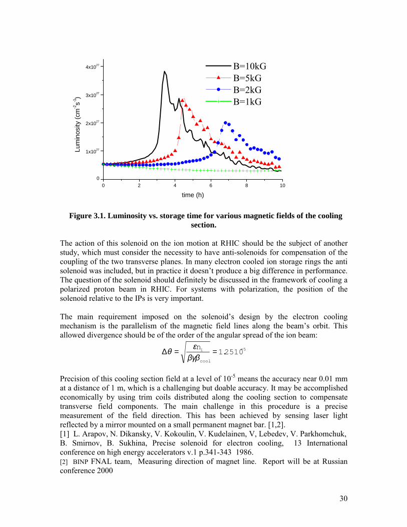
30

0 2 4 6 8 100

1x1027

2x1027

3x1027

4x1027 B=10kG B=5kG B=2kG B=1kG

Lum

inos

ity (c

m-2s-1

)

time (h)

Figure 3.1. Luminosity vs. storage time for various magnetic fields of the coolingsection.

The action of this solenoid on the ion motion at RHIC should be the subject of anotherstudy, which must consider the necessity to have anti-solenoids for compensation of thecoupling of the two transverse planes. In many electron cooled ion storage rings the antisolenoid was included, but in practice it doesn’t produce a big difference in performance.The question of the solenoid should definitely be discussed in the framework of cooling apolarized proton beam in RHIC. For systems with polarization, the position of thesolenoid relative to the IPs is very important.

The main requirement imposed on the solenoid’s design by the electron coolingmechanism is the parallelism of the magnetic field lines along the beam’s orbit. Thisallowed divergence should be of the order of the angular spread of the ion beam:

52510.1 −==∆cool

in

βγβεθ

Precision of this cooling section field at a level of 10-5 means the accuracy near 0.01 mmat a distance of 1 m, which is a challenging but doable accuracy. It may be accomplishedeconomically by using trim coils distributed along the cooling section to compensatetransverse field components. The main challenge in this procedure is a precisemeasurement of the field direction. This has been achieved by sensing laser lightreflected by a mirror mounted on a small permanent magnet bar. [1,2].[1] L. Arapov, N. Dikansky, V. Kokoulin, V. Kudelainen, V, Lebedev, V. Parkhomchuk,B. Smirnov, B. Sukhina, Precise solenoid for electron cooling, 13 Internationalconference on high energy accelerators v.1 p.341-343 1986.[2] BINP FNAL team, Measuring direction of magnet line. Report will be at Russianconference 2000

31

3.1.2 Electron Beam Parameters

For electron cooling of RHIC gold beams it is necessary to have an electron beam with anenergy of 52 MeV, a peak current of up to 0.1 A, an energy spread of Δγ/γ=10-4 and atransverse momentum spread of Δp/p=10-4. In addition to these requirements, thefollowing physics problems must be addressed.

The first problem is matching the length of the electron bunch. Electron bunches from alinear accelerator are very short (Lbunch~1 cm). However, we need bunches with a lengthof about 30 cm. At the same time, increasing the electron bunch length must not lead toan increase in the energy spread by dilution of the longitudinal phase space.

Also, the electron beam from the linear accelerator has an intrinsic energy spread thatmay be too high for cooling. Thus we may adopt the following strategy: The electronbeam will be transformed in longitudinal phase space to produce a longer bunch with thenecessary low energy spread. Then the beam, which still may be shorter than the ionbeam, will be swept in phase to produce coverage of the whole ion bunch. This strategyhas certain advantages; one of them is the ability to control the ion bunch longitudinaldensity distribution. This topic will be discussed in detail later on.

Another problem is introduced by the high value of the cooling section solenoid'smagnetic field (about 1T). The electrons may acquire a high additional transversemomentum upon entering the solenoid. This effect must be corrected by special optics.

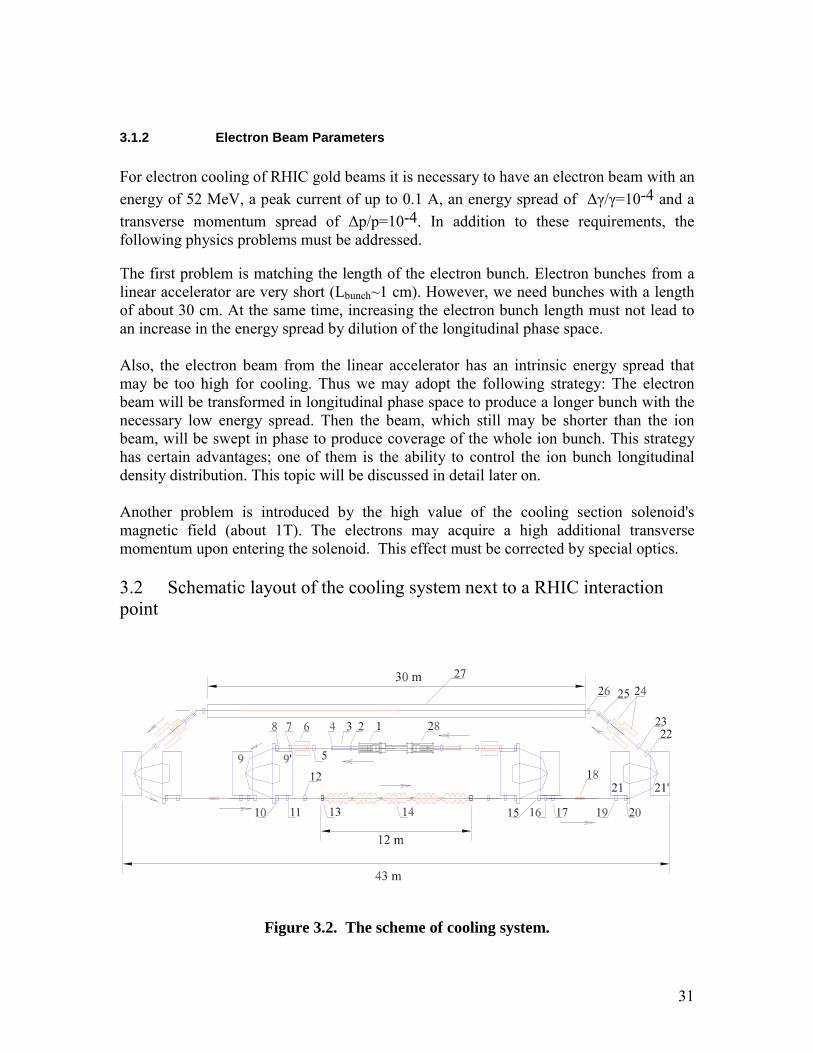
3.2 Schematic layout of the cooling system next to a RHIC interactionpoint

Figure 3.2. The scheme of cooling system.

32

The electron cooling equipment comprises the following key elements:

1 – A 2 MeV injector with a magnetized cathode (the magnetic field on the cathode of theinjector is ~100 G).3 – A solenoid extension of the longitudinal magnetic field of the injector (100 G).2,4 –Skew quadrupoles for the transformation of the magnetized beam into a flat beam6 – Energy modulating cavity for reducing the electron bunch length from 4 ns to 0.06 ns.It consists of two 70 MHz RF-cavity (the gap voltage is 350 kV) and one 210 MHz (36kV) RF-cavity.5,7,8 – Electron optical elements of the bunching system.9,9' – Magnetic compressor (an α-magnet, with a bending radius of 1m).10,11,12,13 – Electron optical elements of the bunching system.14 – RF linac structure (350 MHz LEP structure).15 – A bending magnet for a compensation of the action of the last high-energy (50MeV) bending magnet (9'').18 –Third harmonic of the RF linac (1.05 GHz), for compensation of the non-linearity offundamental accelerating field.16,17,19,20,22,23 – Electron optical elements of the debunching system.21,21' –Magnetic de-compressor (an α-magnet, with a bending radius of 1m).24 –RF-cavity for eliminating the linear energy chirp. It consists of 80 MHz RF cavity(the gap voltage is 4.6 MV) and 240 MHz (0.24 kV). This cavity should besuperconducting.25 – Transfer optics from a flat to a round beam electron beam, for injection into themain solenoid.26 –Bending magnet.27 –Main solenoid (104 G).28 –Beam-dump or system of beam recuperation.

The electron beam from the injector electron gun (2 MeV) with a magnetizedcathode (100 G) is transformed to a flat beam (εnx=2.1⋅10-2 cm⋅rad, εny=7⋅10-4 cm⋅rad).After that, the bunch passes through a bunching section. This section consists of anenergy-modulating RF cavity and an α-magnet magnetic-compressor. The length of theelectron bunch is decreased to the suitable length for acceleration (σz=1.8 cm). In themain linac, the bunch is accelerated to the full energy (52 MeV). The acceleration isdone at a phase of θ= -10° in order to achieve the linear dependence between thelongitudinal momentum and the position of the electron in the bunch (chirp). This chirp isused for further debunching. The length of the electron beam is increased in thedebunching magnet structure up to 10-40 cm, allowing optimization of the cooling. Afterdebunching, the electron beam passes a system of RF cavities designed for reduction ofits momentum spread. Before going into a cooling solenoid the electron beam istransformed from a flat to a round beam. After the cooling section, the beam returns to

33

the debunching system with the necessary modulation of energy for optimization of thebunch length and energy recovery at the main linac. The electron beam with a residualenergy of 2 MeV is terminated in a beam dump.

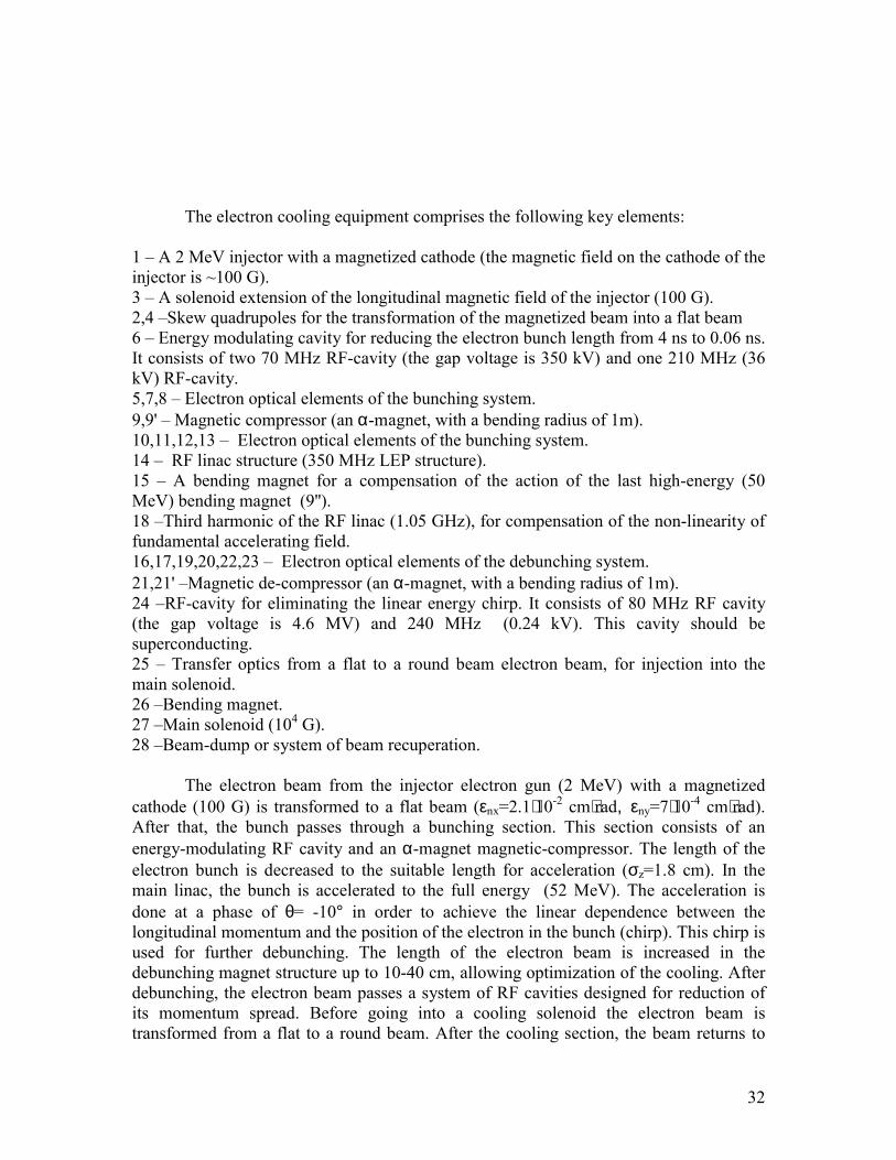
An initial analysis of electron optics has been made using the thin-lensapproximation. The betatron and dispersion function are shown in Figures 3.3 to 3.5. Thedetailed calculation of optic scheme for electron can be completed after a choice ofparameters of electron transport system is made.

In the RF linac structure it is useful to use a special procedure for evaluation ofbetatron function. The motion of particle at acceleration can be written as

)/()(

1012

2

≈=+ cvdsdx

dsd

sdsxd γ

γ. (1)

If we use the Ansatz:

( )

+

′′′

= ∫ 00

2ϕ

γ γγ

s

swssdsAwsx

)(cos)()( . (2)

Then the differential equation becomes:

011322

2

=−+γ

γγ

γγ

γ wdsdw

dsd

sdswd

)( , (3)

which is similar to usual envelop equation. Thus one can calculate the dynamic variablewγ for a given γ(s) and then calculate β(s) as:

2)()()( swss γγβ = . (4)

Figure 3.3. The sketch of betatron and dispersion functions from element 4 to

34

element 13.

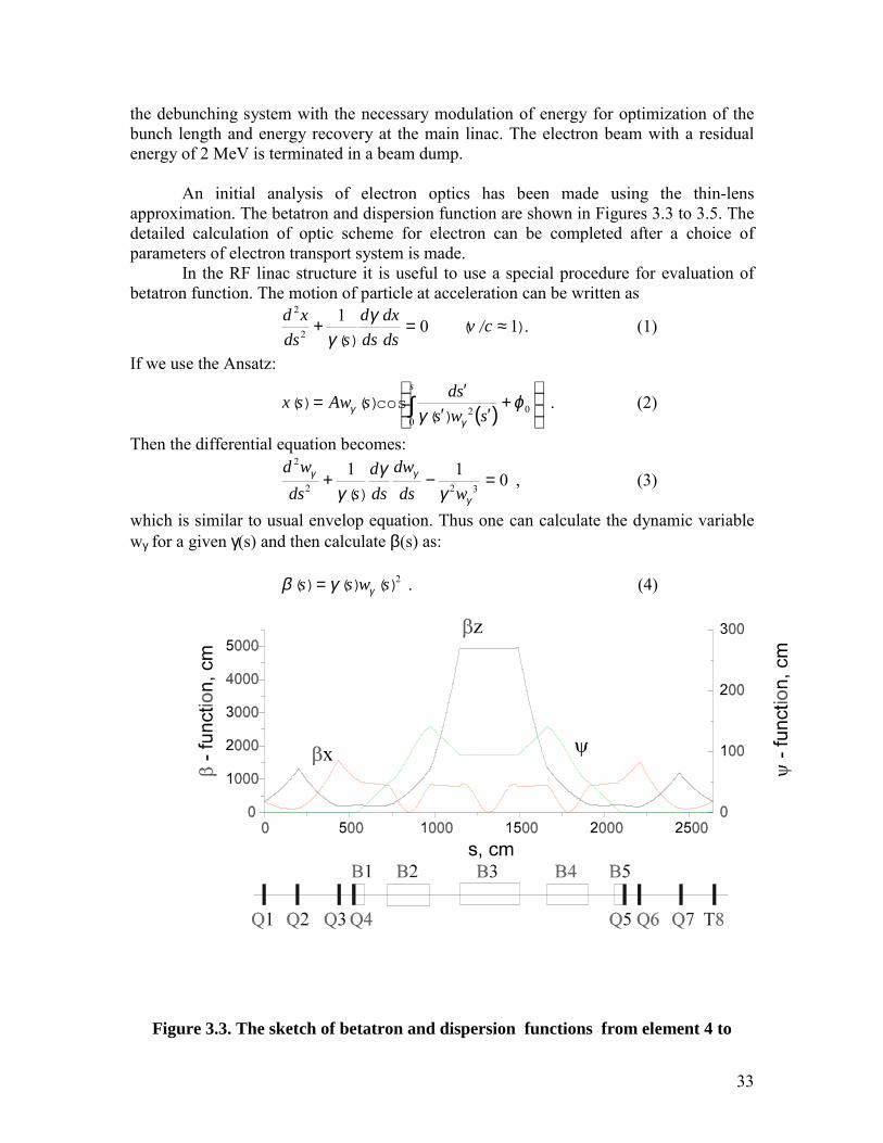
Figure 3.4. The sketch of betatron and dispersion functions from element 13 toelement 21.

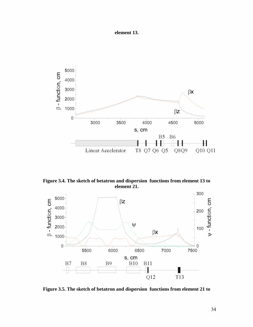
Figure 3.5. The sketch of betatron and dispersion functions from element 21 to

35

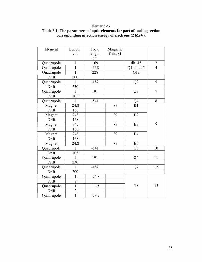
element 25.Table 3.1. The parameters of optic elements for part of cooling section

corresponding injection energy of electrons (2 MeV).

Element Length,cm

Focallength,

cm

Magneticfield, G

Quadrupole 1 169 tilt. 45 2Quadrupole 1 -338 Q1, tilt. 45Quadrupole 1 228 Q1a

4

Drift 200Quadrupole 1 -182 Q2 5

Drift 230Quadrupole 1 191 Q3 7


Magnet 24.8 89 B1Drift 168

Magnet 248 89 B2Drift 168



Magnet 24.8 89 B5

9

Quadrupole 1 -541 Q5 10Drift 105

Quadrupole 1 191 Q6 11Drift 230

Quadrupole 1 -182 Q7 12Drift 200

Quadrupole 1 -24.8Drift 2

Quadrupole 1 11.9Drift 2

Quadrupole 1 -23.9

T8 13

36

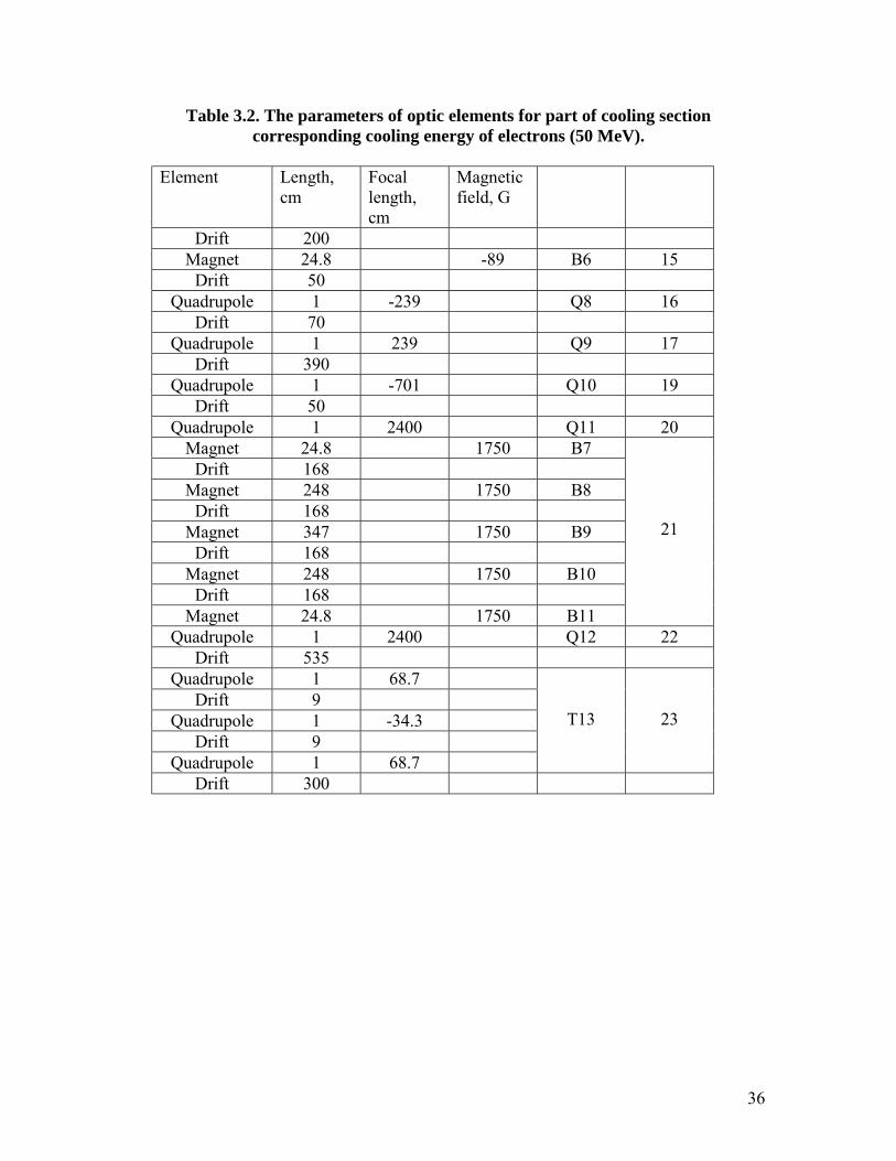
Table 3.2. The parameters of optic elements for part of cooling sectioncorresponding cooling energy of electrons (50 MeV).

Element Length,cm

Focallength,cm

Magneticfield, G

Drift 200Magnet 24.8 -89 B6 15





Magnet 24.8 1750 B7Drift 168




Magnet 24.8 1750 B11

21

Quadrupole 1 2400 Q12 22Drift 535

Quadrupole 1 68.7Drift 9

Quadrupole 1 -34.3Drift 9

Quadrupole 1 68.7

T13 23

Drift 300

37

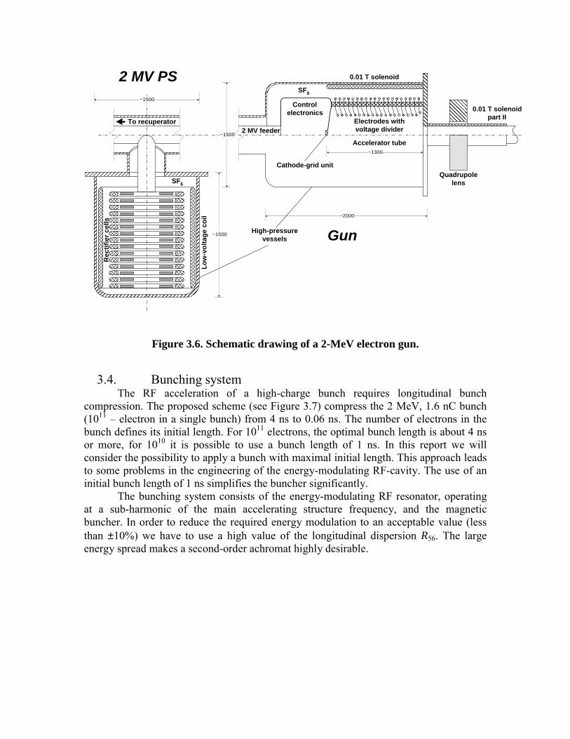
3.3. Electron gun in DC accelerator (2 MeV).

The electron gun design for the 52-MeV electron cooler consists of a high-voltage(2 MV) power supply (PS), controls electronics, and a DC accelerator tube (Figure 3.6).The whole gun is embedded into a high-pressure vessel containing SF6 (≈ 106 Pa). Onecan find some similar devices in [1]...[4]. Its expected parameters are as follows:

Table 3.3. Electron gun parameters.Electron energy (kinetic), MeV 2Relative energy spread 10-3

Average current, mA up to 120Peak current, A 5Pulse duration, ns 4

The design of the high-voltage power supply is based on an AC-transformer with agap in the core to insulate the high voltage from the ground. The operating frequency ischosen to be ~ 1kHz. The low-voltage coil is water-cooled. The inner surface of the high-pressure vessel should be copper-coated to reduce the power loss. Each rectifier cellcontains a coil and high-voltage rectifier. A slow feedback system is used to maintain anexact average-voltage. Ripple is reduced by a fast feedback system with a seriestransformer.

The accelerating tube consists of ceramic rings with brazed electrodes. The tubealso serves as a vacuum chamber. A voltage divider is connected to the electrodes. ALaB6 cathode-grid unit is used as an electron emitter. Its diameter is 25 mm and itsexpected current density is 1.4 A/cm2 (partially absorbed by the grid). The cathodeshould be slightly concave to reduce the temperature dependence on the cathode-to-griddistance. So, some compression inside the gun is necessary. It means that the magnitudeof the magnetic field at the cathode should be lower than its value further along the beamdirection. The cathode-to-grid distance is chosen to be 0.5 mm; the voltage necessary tocontrol the current is ≈ 100 V including the locking voltage. No serious technicalproblems are expected in designing a 100 V, 7 A, 4 ns, and 6 MHz controlled pulser.

Other possibilities for the emitter are: (i) a conventional gridded oxide cathode, (ii)an oxide cathode with a modulating electrode, or (iii) a photo-cathode. A gridded oxidecathode (i) is analogous to the proposed LaB6 one, but it has significantly lowertemperature (advantage) and much greater sensitivity to organic vapor (drawback). Thischoice should be made if one is absolutely sure in absence of organic matter in thevacuum system. Note that the cathode area hardly can be reduced significantly. If thementioned above set of parameters is admitted, the power coming to the grid with theelectrons is ≈ 3.5 W. If the area of the grid is reduced, it can be overheated.

A gridless cathode with a modulating electrode at some distance comparable to thecathode diameter (ii) is much more simple and its area can be much less as there's noproblem with grid overheating in this case. Unfortunately, it claims much higher voltageof the pulser (several kV typically). It's nearly impossible to design a pulser providing,for example, 3 kV 4 ns 5 A pulses with the repetition rate 6 MHz at the current state ofthe art.

38

The third possibility (iii) requires a high-efficiency (~ 1%) photo-cathode and a 30W average power pulsed laser. Note that the length of its optical resonator is to be ≈ 25 mto provide 6 MHz repetition rate. In this case the whole design of the injector ought to berevised as much shorter pulses of much higher current can be obtained (advantage). It'salso known that the life time of such cathodes is too small (typically, several hours), so acathode preparation unit should be included in the gun (drawback).

Both 0.01 T solenoids should be designed to provide the uniform field along theentire axis with the exception of the near-cathode region. There the field should be ≈ 1.5times less to permit the appropriate beam compression. The expected current density is ≈104 A/m, thus the cooling requirement are fulfilled. A quadrupole lens over the secondsolenoid is necessary to convert the round beam into a flat beam outside the magneticfield.

The control electronics should contain a set of controlled power supplies forfilament, bias, and the pulser. The requirement for the timing jitter of the pulser trigger isless than 0.3 ns. One should pay particular attention to the cooling of the gun. Theexpected power dissipation is ~ 300 W in the cathode and ~ 30 kW in the high-voltagepower supply.

References[1] M.L. Sundquist, R.D. Rathmell, and J.E. Raatz. NIM A287 (1990) 87-89.[2] J.E. Raatz, R.D. Rathmell, P.H. Stelson and N.F. Ziegler. NIM A244 (1986) 104-

106.[3] Industrial electron accelerators of ELV type. http://www.inp.nsk.su/products/indaccel/elv.en.shtml.

[4] B.B.Baklakov, A.M.Batrakov, et al. Status of the Free Electron Laser for theSiberian Centre for Photochemical Research. SR'2000, Novosibirsk, Russia (oral, tobe published in the SR'2000 Proceedings in NIM).

High-pressurevessels

Rec

tifie

r cel

ls

Low

-vol

tage

coi

l

Controlelectronics

Cathode-grid unit

0.01 T solenoid

Accelerator tube

Electrodes withvoltage divider

0.01 T solenoidpart II

Quadrupolelens

~2000

~1300

SF6

2 MV feeder

~1500

~1500

2 MV PS

~1500

Gun

To recuperator

SF6

Figure 3.6. Schematic drawing of a 2-MeV electron gun.

3.4. Bunching systemThe RF acceleration of a high-charge bunch requires longitudinal bunch

compression. The proposed scheme (see Figure 3.7) compress the 2 MeV, 1.6 nC bunch(1011 – electron in a single bunch) from 4 ns to 0.06 ns. The number of electrons in thebunch defines its initial length. For 1011 electrons, the optimal bunch length is about 4 nsor more, for 1010 it is possible to use a bunch length of 1 ns. In this report we willconsider the possibility to apply a bunch with maximal initial length. This approach leadsto some problems in the engineering of the energy-modulating RF-cavity. The use of aninitial bunch length of 1 ns simplifies the buncher significantly.

The bunching system consists of the energy-modulating RF resonator, operatingat a sub-harmonic of the main accelerating structure frequency, and the magneticbuncher. In order to reduce the required energy modulation to an acceptable value (lessthan ±10%) we have to use a high value of the longitudinal dispersion R56. The largeenergy spread makes a second-order achromat highly desirable.

40

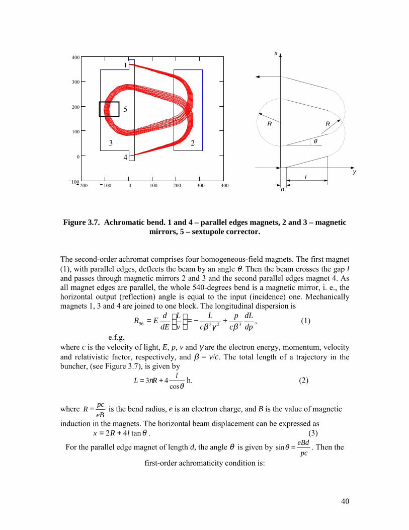
Figure 3.7. Achromatic bend. 1 and 4 – parallel edges magnets, 2 and 3 – magneticmirrors, 5 – sextupole corrector.

The second-order achromat comprises four homogeneous-field magnets. The first magnet(1), with parallel edges, deflects the beam by an angle θ. Then the beam crosses the gap land passes through magnetic mirrors 2 and 3 and the second parallel edges magnet 4. Asall magnet edges are parallel, the whole 540-degrees bend is a magnetic mirror, i. e., thehorizontal output (reflection) angle is equal to the input (incidence) one. Mechanicallymagnets 1, 3 and 4 are joined to one block. The longitudinal dispersion is

dpdL

cp

cL

vL

dEdER 32356 βγβ

+−=

= , (1)

e.f.g.where c is the velocity of light, E, p, v and γ are the electron energy, momentum, velocityand relativistic factor, respectively, and β = v/c. The total length of a trajectory in thebuncher, (see Figure 3.7), is given by

θπ

cos43 lRL += h. (2)

where eBpcR = is the bend radius, e is an electron charge, and B is the value of magnetic

induction in the magnets. The horizontal beam displacement can be expressed asθtan42 lRx += . (3)

For the parallel edge magnet of length d, the angle θ is given by pc

eBd=θsin . Then the

first-order achromaticity condition is:

y

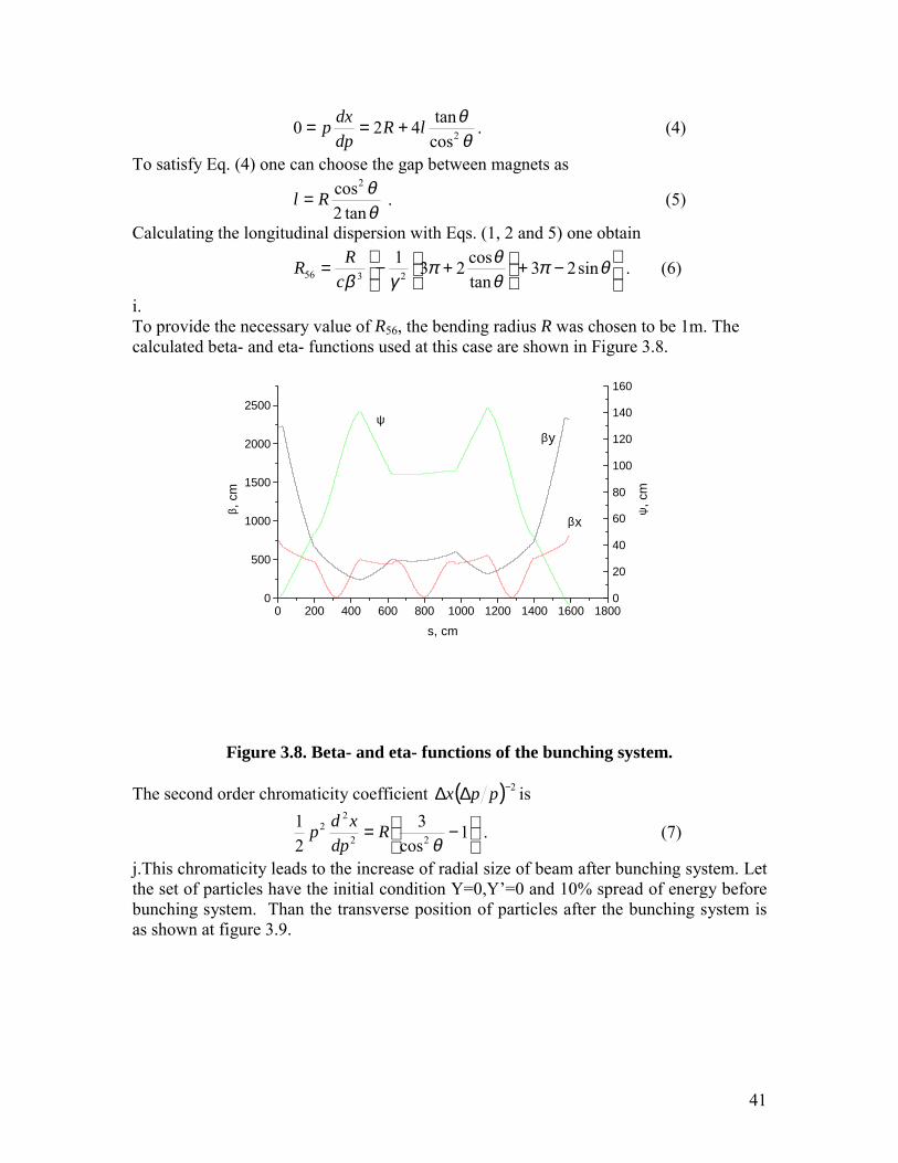
x

RR

θ

l

d200 100 0 100 200 300 400100

0

100

200

300

400

2

1

4

3

5

41

θθ

2costan420 lR

dpdxp +== . (4)

To satisfy Eq. (4) one can choose the gap between magnets as

θθ

tan2cos2

Rl = . (5)

Calculating the longitudinal dispersion with Eqs. (1, 2 and 5) one obtain

−+

+−= θπ

θθπ

γβsin23

tancos231

2356 cRR . (6)

i.To provide the necessary value of R56, the bending radius R was chosen to be 1m. Thecalculated beta- and eta- functions used at this case are shown in Figure 3.8.

Figure 3.8. Beta- and eta- functions of the bunching system.

The second order chromaticity coefficient ( ) 2−∆∆ ppx is

−= 1

cos3

21

22

22

θR

dpxdp . (7)

j.This chromaticity leads to the increase of radial size of beam after bunching system. Letthe set of particles have the initial condition Y=0,Y’=0 and 10% spread of energy beforebunching system. Than the transverse position of particles after the bunching system isas shown at figure 3.9.

0 200 400 600 800 1000 1200 1400 1600 18000

500

1000

1500

2000

2500

β , c

m

s, cm

0

20

40

60

80

100

120

140

160

ψ, c

m

ψ

βx

βy

42

4.5 5 5.5191

191.75

192.5

193.25

194

Energy

Y '

.

Y

Figure 3.9. The transverse position of electron versus energy (γγγγ=E/mc2).

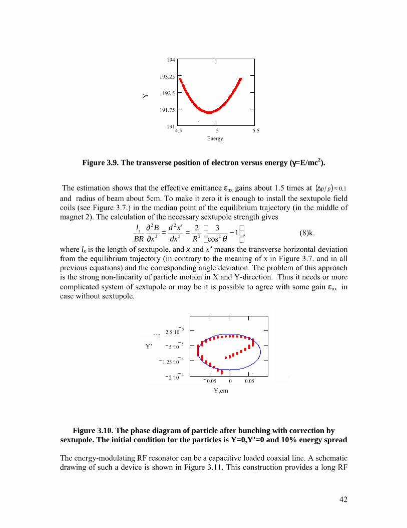
The estimation shows that the effective emittance εnx gains about 1.5 times at ( ) 1.0≈∆ pp

and radius of beam about 5cm. To make it zero it is enough to install the sextupole fieldcoils (see Figure 3.7.) in the median point of the equilibrium trajectory (in the middle ofmagnet 2). The calculation of the necessary sextupole strength gives

−=

′=

∂∂ 1

cos32

222

2

2

2

θRdxxd

xB

BRls , (8)k.

where ls is the length of sextupole, and x and x’ means the transverse horizontal deviationfrom the equilibrium trajectory (in contrary to the meaning of x in Figure 3.7. and in allprevious equations) and the corresponding angle deviation. The problem of this approachis the strong non-linearity of particle motion in X and Y-direction. Thus it needs or morecomplicated system of sextupole or may be it is possible to agree with some gain εnx incase without sextupole.

Figure 3.10. The phase diagram of particle after bunching with correction bysextupole. The initial condition for the particles is Y=0,Y’=0 and 10% energy spread

The energy-modulating RF resonator can be a capacitive loaded coaxial line. A schematicdrawing of such a device is shown in Figure 3.11. This construction provides a long RF

194.5

4.75

5

5.25

5.5

0.05 0 0.05 2 . 10 4

1.25 . 10 4

5 . 10 5

2.5 . 10 5

Yfinish (cm)

Yfinish '

.

Emitt π a ⋅ b ⋅ := Emitt 2.262 10 5 − × = Y,cm

Y’

43

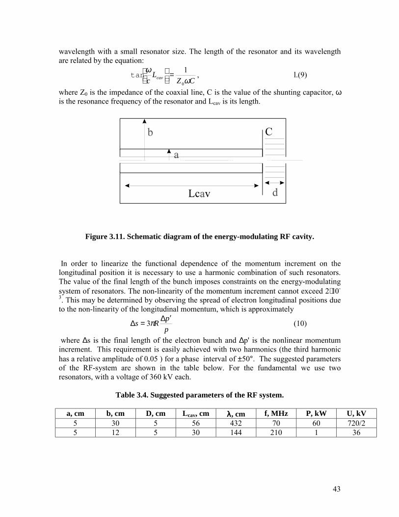
wavelength with a small resonator size. The length of the resonator and its wavelengthare related by the equation:

CZL

c cav ωω

0

1=

tan , l.(9)

where Z0 is the impedance of the coaxial line, C is the value of the shunting capacitor, ωis the resonance frequency of the resonator and Lcav is its length.

Figure 3.11. Schematic diagram of the energy-modulating RF cavity.

In order to linearize the functional dependence of the momentum increment on thelongitudinal position it is necessary to use a harmonic combination of such resonators.The value of the final length of the bunch imposes constraints on the energy-modulatingsystem of resonators. The non-linearity of the momentum increment cannot exceed 2⋅10-

3. This may be determined by observing the spread of electron longitudinal positions dueto the non-linearity of the longitudinal momentum, which is approximately

ppRs′∆=∆ π3 (10)

where ∆s is the final length of the electron bunch and ∆p' is the nonlinear momentumincrement. This requirement is easily achieved with two harmonics (the third harmonichas a relative amplitude of 0.05 ) for a phase interval of ±50°. The suggested parametersof the RF-system are shown in the table below. For the fundamental we use tworesonators, with a voltage of 360 kV each.

Table 3.4. Suggested parameters of the RF system.

a, cm b, cm D, cm Lcav, cm λλλλ, cm f, MHz P, kW U, kV5 30 5 56 432 70 60 720/25 12 5 30 144 210 1 36

44

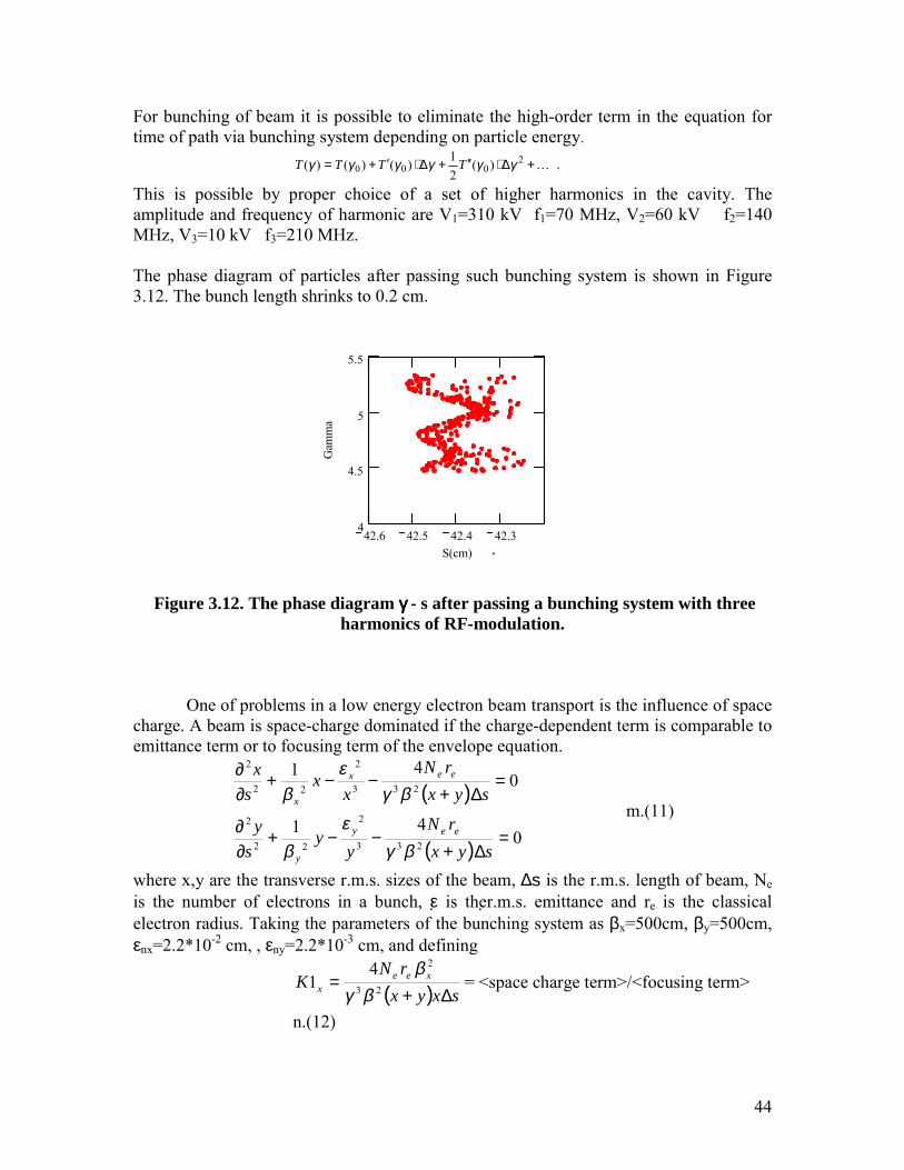
For bunching of beam it is possible to eliminate the high-order term in the equation fortime of path via bunching system depending on particle energy.

"+∆⋅′′+∆⋅′+= 2000 )(

21)()()( γγγγγγ TTTT .

This is possible by proper choice of a set of higher harmonics in the cavity. Theamplitude and frequency of harmonic are V1=310 kV f1=70 MHz, V2=60 kV f2=140MHz, V3=10 kV f3=210 MHz.

The phase diagram of particles after passing such bunching system is shown in Figure3.12. The bunch length shrinks to 0.2 cm.

Figure 3.12. The phase diagram γγγγ - s after passing a bunching system with threeharmonics of RF-modulation.

One of problems in a low energy electron beam transport is the influence of spacecharge. A beam is space-charge dominated if the charge-dependent term is comparable toemittance term or to focusing term of the envelope equation.

( )

( ) 041

041

233

2

22

2

233

2

22

2

=∆+

−−+∂∂

=∆+

−−+∂∂

syxrN

yy

sy

syxrN

xx

sx

eey

y

eex

x

βγε

β

βγε

β m.(11)

where x,y are the transverse r.m.s. sizes of the beam, ∆s is the r.m.s. length of beam, Neis the number of electrons in a bunch, ε is ther.m.s. emittance and re is the classicalelectron radius. Taking the parameters of the bunching system as βx=500cm, βy=500cm,εnx=2.2*10-2 cm, , εny=2.2*10-3 cm, and defining

( ) sxyxrN

K xeex ∆+

= 23

241

βγβ

= <space charge term>/<focusing term>

n.(12)

42.6 42.5 42.4 42.34

4.5

5

5.5

S(cm)

Gam

ma

.

45

( ) 2

342

xn

eex

syx

xrNK

εγ ∆+= = <space charge term>/<emittance term>

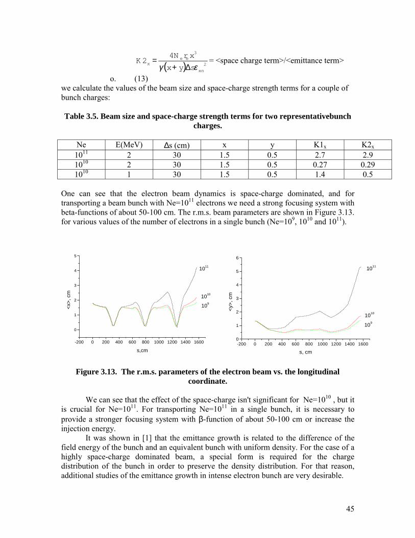
o. (13)we calculate the values of the beam size and space-charge strength terms for a couple ofbunch charges:

Table 3.5. Beam size and space-charge strength terms for two representativebunchcharges.

Ne E(MeV) ∆s (cm) x y K1x K2x

1011 2 30 1.5 0.5 2.7 2.91010 2 30 1.5 0.5 0.27 0.291010 1 30 1.5 0.5 1.4 0.5

One can see that the electron beam dynamics is space-charge dominated, and fortransporting a beam bunch with Ne=1011 electrons we need a strong focusing system withbeta-functions of about 50-100 cm. The r.m.s. beam parameters are shown in Figure 3.13.for various values of the number of electrons in a single bunch (Ne=109, 1010 and 1011).

Figure 3.13. The r.m.s. parameters of the electron beam vs. the longitudinalcoordinate.

We can see that the effect of the space-charge isn't significant for Ne=1010 , but itis crucial for Ne=1011. For transporting Ne=1011 in a single bunch, it is necessary toprovide a stronger focusing system with β-function of about 50-100 cm or increase theinjection energy.

It was shown in [1] that the emittance growth is related to the difference of thefield energy of the bunch and an equivalent bunch with uniform density. For the case of ahighly space-charge dominated beam, a special form is required for the chargedistribution of the bunch in order to preserve the density distribution. For that reason,additional studies of the emittance growth in intense electron bunch are very desirable.

-200 0 200 400 600 800 1000 1200 1400 1600

0

1

2

3

4

5

109

1010

1011

<x>,

cm

s,cm-200 0 200 400 600 800 1000 1200 1400 16000

1

2

3

4

5

6

109

1010

1011

<y>,

cm

s, cm

46

Another problem for high-charge bunch is the physics of such a bunch in adispersion element (bend). The space-charge force can add a correlation between thehorizontal position of electron and its longitudinal momentum. This effect vanishes at ahigh electron energy.

1. I. Hofmann and J. Struckmeier. Generalized three-dimensional equations for theemittance and field energy of high-current beams in periodic focusing structures. ParticleAccelerators, 1987, Vol.21., pp.69-98.

3.5 Main linac

For electron cooling of RHIC we need an electron beam with an energy of 52MeV, more than 1010 electrons in a single bunch, an energy spread of ∆γ/γ=10-4 or betterand a transverse momentum spread of ∆p⊥ /p=4⋅10-4 or better. The main factors affectingthe energy and momentum spread of the electron beam in a linear accelerator are thefollowing:

1. Wake field produced by higher-order modes of the cavity on the energyspread of particles.

2. The time dependence of the accelerating RF voltage during the passage of ashort electron bunch.

3. The influence of a space-charge field on the energy spread of particles.4. The influence of inhomogeneity of the magnetic and transverse electric

components on the particle’s motion.The bunch is placed at a phase of θ= -10° in order to produce a linear correlation betweenthe longitudinal momentum and position in the bunch (chirp). This chirp will later servefor debunching of the electrons.

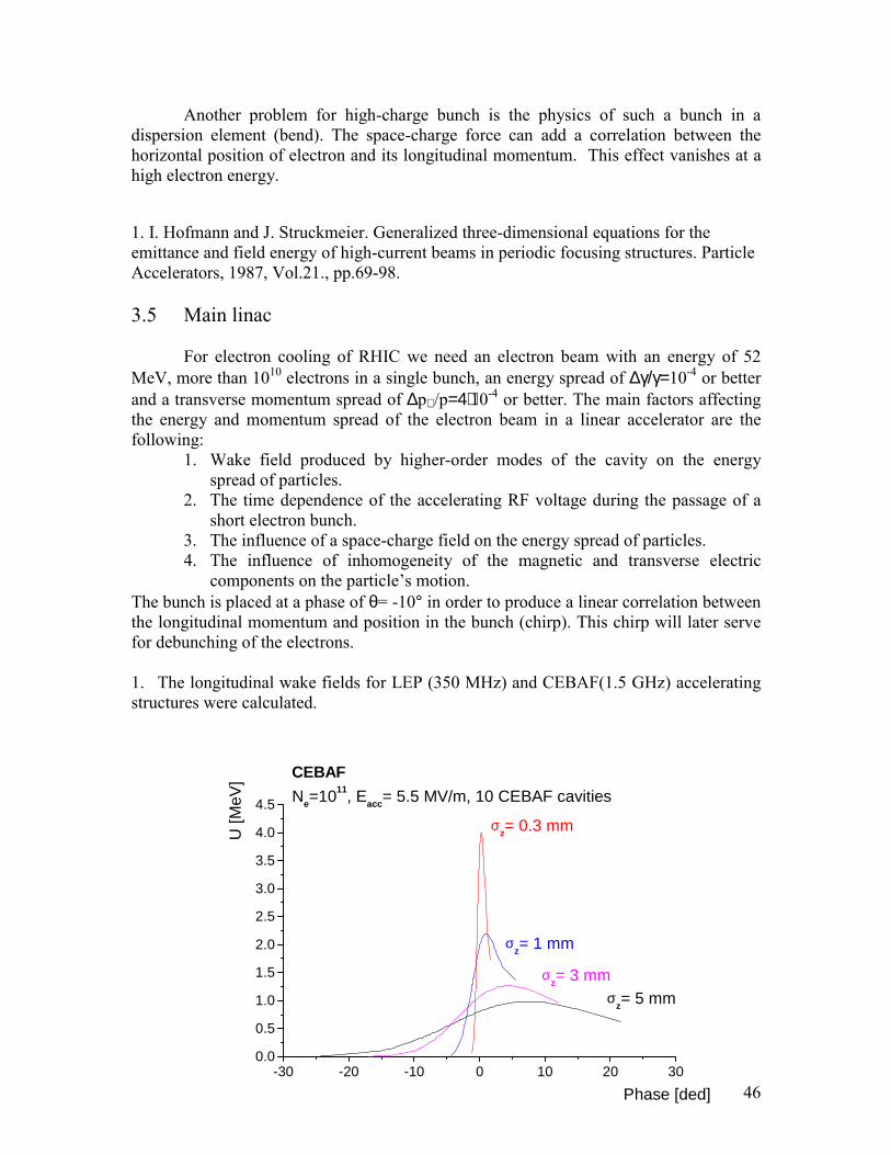
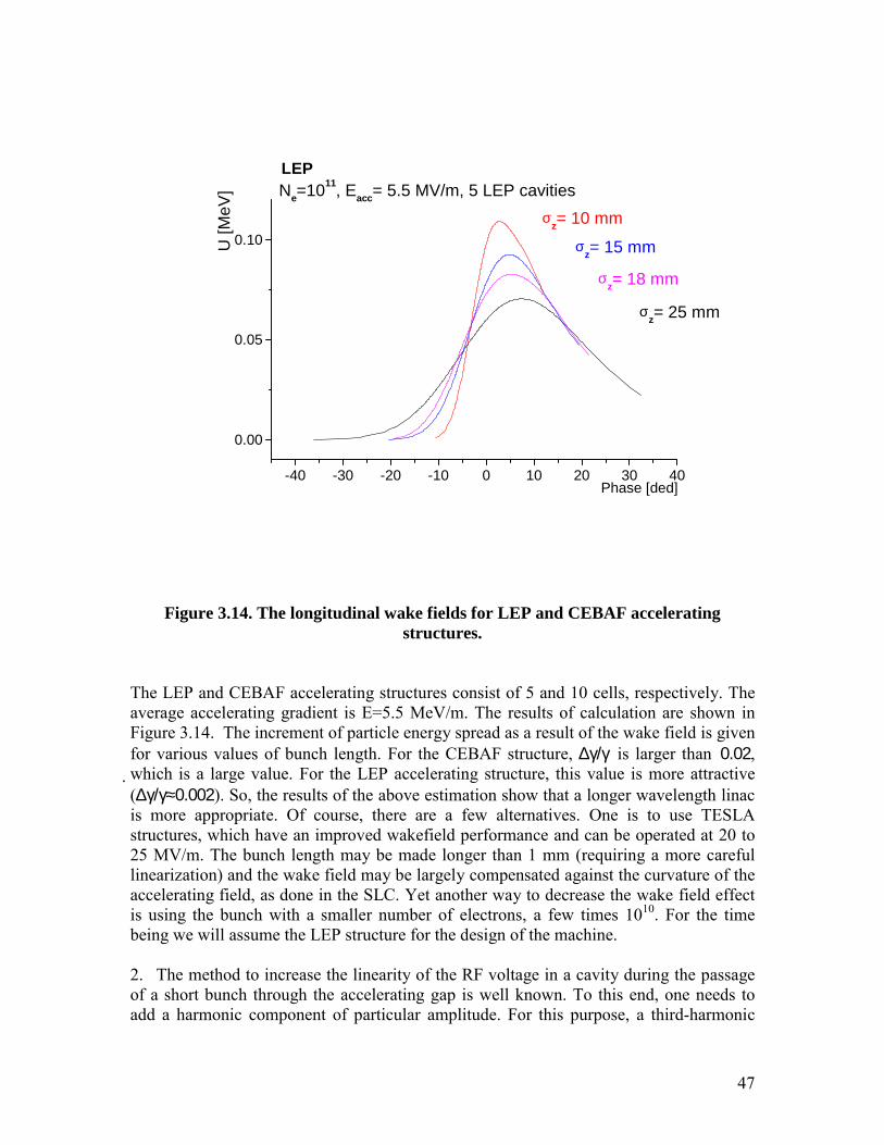
1. The longitudinal wake fields for LEP (350 MHz) and CEBAF(1.5 GHz) acceleratingstructures were calculated.

-30 -20 -10 0 10 20 300.0

0.5

1.0

1.5

2.0

2.5

3.0

3.5

4.0

4.5 Ne=1011, Eacc= 5.5 MV/m, 10 CEBAF cavities

σz= 0.3 mm

σz= 1 mm

σz= 3 mm σz= 5 mm

CEBAF

U [M

eV]

Phase [ded]

47

Figure 3.14. The longitudinal wake fields for LEP and CEBAF acceleratingstructures.

The LEP and CEBAF accelerating structures consist of 5 and 10 cells, respectively. Theaverage accelerating gradient is E=5.5 MeV/m. The results of calculation are shown inFigure 3.14. The increment of particle energy spread as a result of the wake field is givenfor various values of bunch length. For the CEBAF structure, ∆γ/γ is larger than 0.02,which is a large value. For the LEP accelerating structure, this value is more attractive(∆γ/γ≈0.002). So, the results of the above estimation show that a longer wavelength linacis more appropriate. Of course, there are a few alternatives. One is to use TESLAstructures, which have an improved wakefield performance and can be operated at 20 to25 MV/m. The bunch length may be made longer than 1 mm (requiring a more carefullinearization) and the wake field may be largely compensated against the curvature of theaccelerating field, as done in the SLC. Yet another way to decrease the wake field effectis using the bunch with a smaller number of electrons, a few times 1010. For the timebeing we will assume the LEP structure for the design of the machine.

2. The method to increase the linearity of the RF voltage in a cavity during the passageof a short bunch through the accelerating gap is well known. To this end, one needs toadd a harmonic component of particular amplitude. For this purpose, a third-harmonic

-40 -30 -20 -10 0 10 20 30 40

0.00

0.05

0.10

Ne=1011, Eacc= 5.5 MV/m, 5 LEP cavitiesLEP

σz= 25 mm

σz= 18 mm

σz= 15 mm

σz= 10 mm U

[MeV

]

Phase [ded]

48

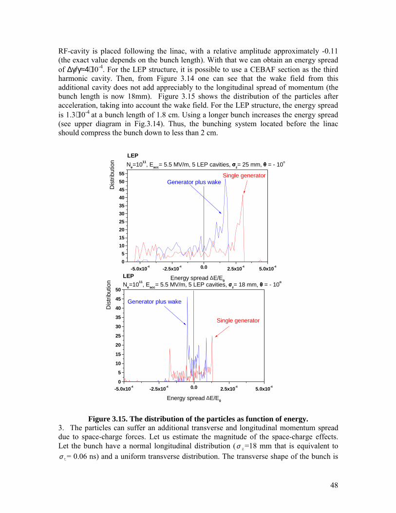
RF-cavity is placed following the linac, with a relative amplitude approximately -0.11(the exact value depends on the bunch length). With that we can obtain an energy spreadof ∆γ/γ≈4⋅10-4. For the LEP structure, it is possible to use a CEBAF section as the thirdharmonic cavity. Then, from Figure 3.14 one can see that the wake field from thisadditional cavity does not add appreciably to the longitudinal spread of momentum (thebunch length is now 18mm). Figure 3.15 shows the distribution of the particles afteracceleration, taking into account the wake field. For the LEP structure, the energy spreadis 1.3⋅10-4 at a bunch length of 1.8 cm. Using a longer bunch increases the energy spread(see upper diagram in Fig.3.14). Thus, the bunching system located before the linacshould compress the bunch down to less than 2 cm.

Figure 3.15. The distribution of the particles as function of energy.3. The particles can suffer an additional transverse and longitudinal momentum spreaddue to space-charge forces. Let us estimate the magnitude of the space-charge effects.Let the bunch have a normal longitudinal distribution ( zσ =18 mm that is equivalent to

tσ = 0.06 ns) and a uniform transverse distribution. The transverse shape of the bunch is

-5.0x10-4 -2.5x10-4 0.0 2.5x10-4 5.0x10-40

5

10

15

20

25

30

35

40

45

50

Generator plus wake

Single generator

Ne=1011, Eacc= 5.5 MV/m, 5 LEP cavities, σσσσz= 18 mm, θθθθ = - 10oLEP

Dis

tribu

tion

Energy spread ∆E/E0

-5.0x10-4 -2.5x10-4 0.0 2.5x10-4 5.0x10-405

10152025303540455055

Generator plus wakeSingle generator

Ne=1011, Eacc= 5.5 MV/m, 5 LEP cavities, σσσσz= 25 mm, θθθθ = - 10oLEP

Dis

tribu

tion

Energy spread ∆E/E0

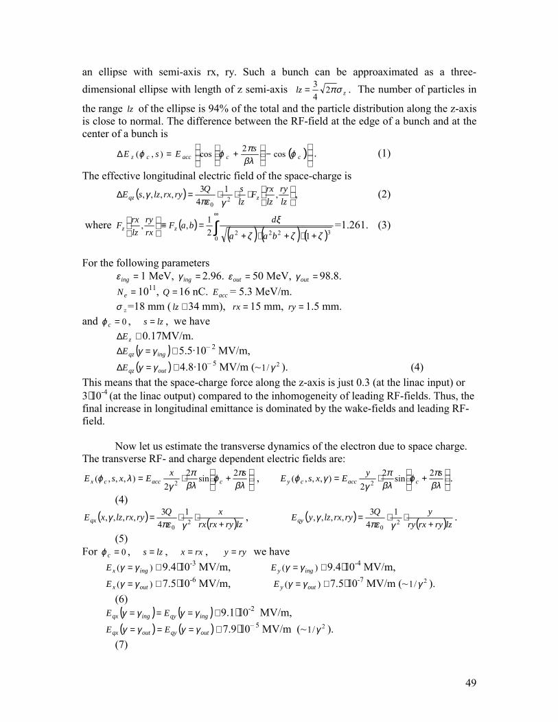
49

an ellipse with semi-axis rx, ry. Such a bunch can be approaximated as a three-dimensional ellipse with length of z semi-axis zlz σπ2

43= . The number of particles in

the range lz of the ellipse is 94% of the total and the particle distribution along the z-axisis close to normal. The difference between the RF-field at the edge of a bunch and at thecenter of a bunch is

( )

−

+=∆ ccacccz

sEsE ϕβλπϕϕ cos2cos),( . (1)

The effective longitudinal electric field of the space-charge is

( )

⋅⋅⋅=∆

lzry

lzrxF

lzsQryrxlzsE zqz ,1

43,,,, 2

0 γπεγ , (2)

where ( ) ( ) ( ) ( )∫∞

+⋅+⋅+=≡

03222 12

1,,ζζζ

ξ

baa

dbaFrxry

lzrxF zz =1.261. (3)

For the following parameters=ingε 1 MeV, =ingγ 2.96. =outε 50 MeV, =outγ 98.8.=eN 1011, =Q 16 nC. accE = 5.3 MeV/m.

zσ =18 mm ( ≅lz 34 mm), =rx 15 mm, =ry 1.5 mm.and 0=cϕ , lzs = , we have

≅∆ zE 0.17MV/m.( ) ≅=∆ ingqzE γγ 5.5·10– 2 MV/m,( ) ≅=∆ outqzE γγ 4.8·10– 5 MV/m (~ 2/1 γ ). (4)

This means that the space-charge force along the z-axis is just 0.3 (at the linac input) or3⋅10-4 (at the linac output) compared to the inhomogeneity of leading RF-fields. Thus, thefinal increase in longitudinal emittance is dominated by the wake-fields and leading RF-field.

Now let us estimate the transverse dynamics of the electron due to space charge.The transverse RF- and charge dependent electric fields are:

+⋅=

βλπϕ

βλπ

γλϕ sxExsE cacccx

2sin22

),,,( 2 ,

+⋅=

βλπϕ

βλπ

γγϕ syExsE cacccy

2sin22

),,,( 2 .

(4)( ) ( )lzryrxrx

xQryrxlzxEqx +⋅⋅= 2

0

143,,,,

γπεγ , ( ) ( )lzryrxry

yQryrxlzyEqy +⋅⋅= 2

0

143,,,,

γπεγ .

(5)For 0=cϕ , lzs = , rxx = , ryy = we have ≅= )( ingxE γγ 9.4⋅10-3 MV/m, ≅= )( ingyE γγ 9.4⋅10-4 MV/m, ≅= )( outxE γγ 7.5⋅10-6 MV/m, ≅= )( outyE γγ 7.5⋅10-7 MV/m (~ 2/1 γ ).

(6) ( ) ( ) ≅=== ingqyingqx EE γγγγ 9.1⋅10-2 MV/m, ( ) ( ) ≅=== outqyoutqx EE γγγγ 7.9⋅10– 5 MV/m (~ 2/1 γ ).

(7)

50

In contrast to the case of longitudinal dynamics, the space-charge force dominates thetransverse dynamics of the electrons.

The calculation above shows that the accelerating rate of 5.3 MeV/m is sufficient toinsure the invariability of the bunch length during acceleration considering the space-charge force.

Note that at a first glance, it would seem that the range of short wave length ismore attractive, as its overall dimensions are relatively small as well as its cost. But∆p||/p∼σ z

3∼ω 03, where ω0 is the main frequency. Thus the difficulties related to the effect

of space-charge force are sharply increased with an increase in the accelerator workingfrequency. Therefore we should use the minimum RF frequency.

3.6 Debunching system after linac.The length of electron bunches is very short (Lbunch~1cm). However, for

electron cooling we need bunches with a length of about 30 cm. The debuncher is similarto the buncher device at low energy (section 3.4). It consists of the energy-modulating RFand the magnetic buncher. The buncher with a high value of the longitudinal dispersion isrequired for decreasing RF voltage needed for the reduction of momentum spread ofelectron. In this report we use a 4% modulation of energy for debunching. It is alsopossible to use 1-0.5% but this variant will have a magnet of large size. In theintermediate report we considered the variants with a half-turn bend bunching system.Similar bunchers have the large size and we have now chosen the α- magnet system as adispersion element.

We use the result of the section 3.4. The total length of trajectory in a buncher(Fig.3.7. in section 3.4.) is:

θπ

cos43 lRL += (1)

This system produces a bunch of about 30 cm in length for a bend radius 1 m and arelative momentum spread of Δp/p0 = 0.04.

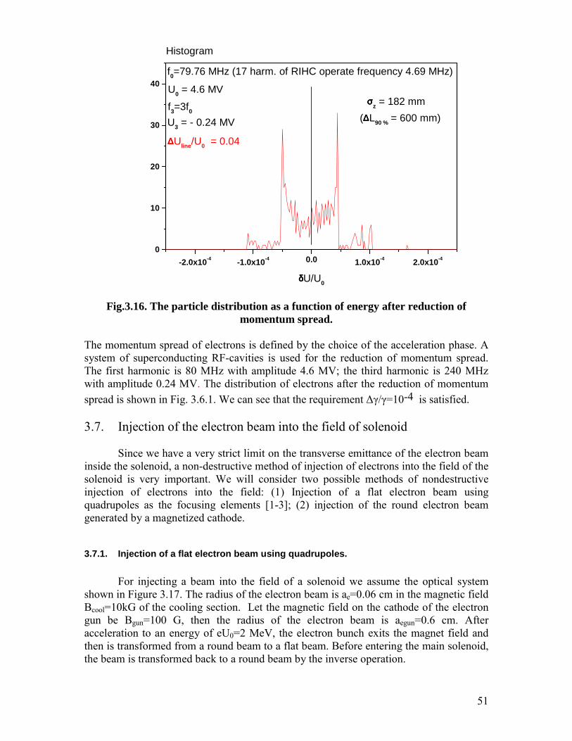
51

Fig.3.16. The particle distribution as a function of energy after reduction ofmomentum spread.

The momentum spread of electrons is defined by the choice of the acceleration phase. Asystem of superconducting RF-cavities is used for the reduction of momentum spread.The first harmonic is 80 MHz with amplitude 4.6 MV; the third harmonic is 240 MHzwith amplitude 0.24 MV. The distribution of electrons after the reduction of momentumspread is shown in Fig. 3.6.1. We can see that the requirement Δγ/γ=10-4 is satisfied.

3.7. Injection of the electron beam into the field of solenoid

Since we have a very strict limit on the transverse emittance of the electron beaminside the solenoid, a non-destructive method of injection of electrons into the field of thesolenoid is very important. We will consider two possible methods of nondestructiveinjection of electrons into the field: (1) Injection of a flat electron beam usingquadrupoles as the focusing elements [1-3]; (2) injection of the round electron beamgenerated by a magnetized cathode.

3.7.1. Injection of a flat electron beam using quadrupoles.

For injecting a beam into the field of a solenoid we assume the optical systemshown in Figure 3.17. The radius of the electron beam is ae=0.06 cm in the magnetic fieldBcool=10kG of the cooling section. Let the magnetic field on the cathode of the electrongun be Bgun=100 G, then the radius of the electron beam is aegun=0.6 cm. Afteracceleration to an energy of eU0=2 MeV, the electron bunch exits the magnet field andthen is transformed from a round beam to a flat beam. Before entering the main solenoid,the beam is transformed back to a round beam by the inverse operation.

-2.0x10-4 -1.0x10-4 0.0 1.0x10-4 2.0x10-40

10

20

30

40

(∆∆∆∆L90 % = 600 mm)σσσσz = 182 mm

∆∆∆∆Uline/U0 = 0.04

U3 = - 0.24 MVf3=3f0

U0 = 4.6 MV

f0=79.76 MHz (17 harm. of RIHC operate frequency 4.69 MHz)

Histogram

δδδδU/U0

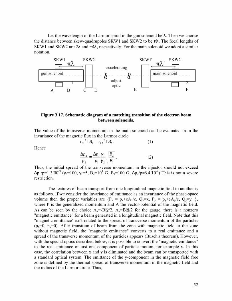
52

Let the wavelength of the Larmor spiral in the gun solenoid be λ. Then we choosethe distance between skew-quadrupoles SKW1 and SKW2 to be πλ. The focal lengths ofSKW1 and SKW2 are 2λ and −4λ, respectively. For the main solenoid we adopt a similarnotation.

Figure 3.17. Schematic diagram of a matching transition of the electron beambetween solenoids.

The value of the transverse momentum in the main solenoid can be evaluated from theinvariance of the magnetic flux in the Larmor circle

22

212

1 BrBr LL ⋅=⋅ . (1)Hence

1

2

2

1

1

1

2

2

BB

pp

pp

γγ∆

=∆

. (2)

Thus, the initial spread of the transverse momentum in the injector should not exceed∆p1/p=1.3⋅10-3 (γ2=100, γ1=5, B2=104 G, B1=100 G, ∆p2/p≈6.4⋅10-4) This is not a severerestriction.

The features of beam transport from one longitudinal magnetic field to another isas follows. If we consider the invariance of emittance as an invariance of the phase-spacevolume then the proper variables are Px = px+eAx/c, Qx=x, Py = py+eAy/c, Qy=y, ,where P is the generalized momentum and A the vector-potential of the magnetic field.As can be seen by the choice Ax=-B⋅y/2, Ay=B⋅x/2 for the gauge, there is a nonzero"magnetic emittance" for a beam generated in a longitudinal magnetic field. Note that this"magnetic emittance" isn't related to the spread of transverse momentum of the particles(px=0, py=0). After transition of beam from the zone with magnetic field to the zonewithout magnetic field, the "magnetic emittance" converts to a real emittance and aspread of the transverse momentum of the particles appears (Busch's theorem). However,with the special optics described below, it is possible to convert the "magnetic emittance"to the real emittance of just one component of particle motion, for example x. In thiscase, the correlation between x and y is eliminated and the beam can be transported witha standard optical system. The emittance of the y-component in the magnetic field freezone is defined by the thermal spread of transverse momentum in the magnetic field andthe radius of the Larmor circle. Thus,

1 2A B C D E F

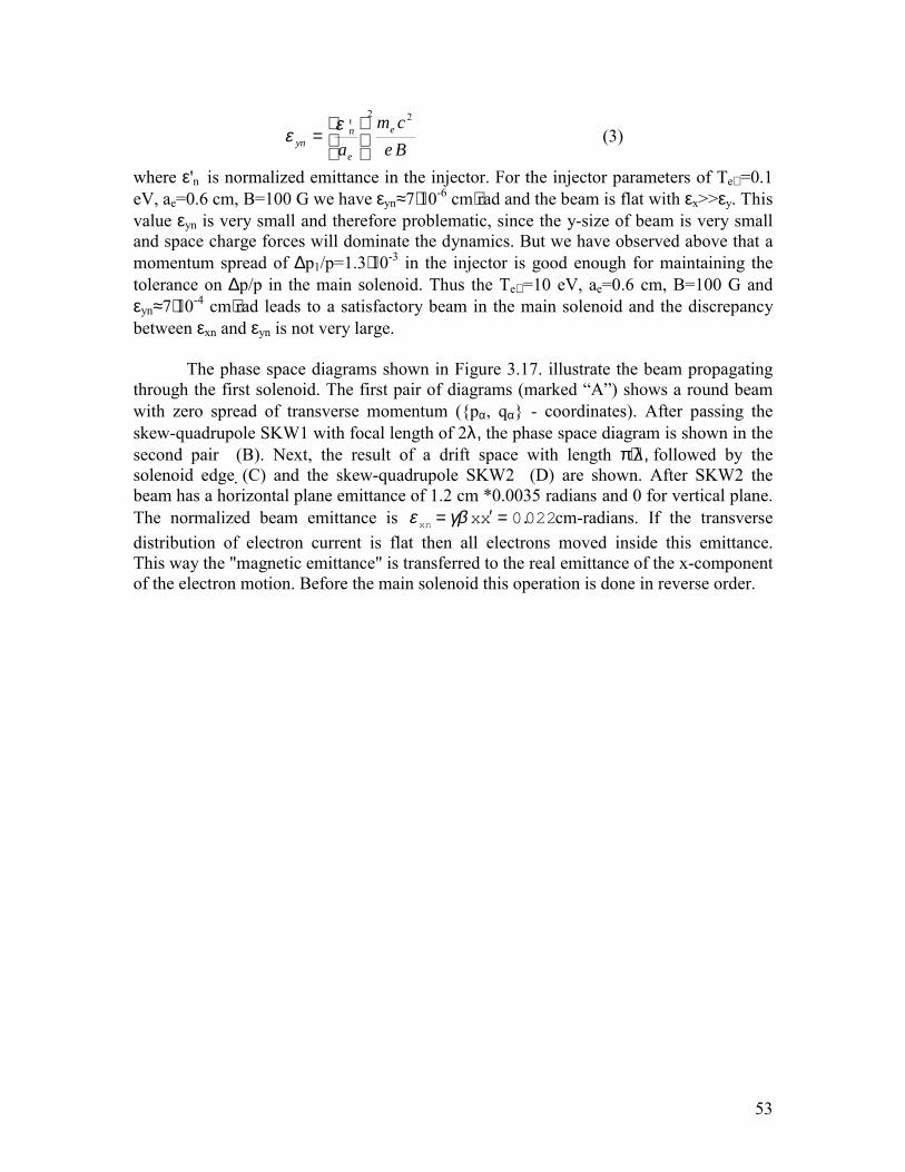
53

Becm

ae

e

nyn

22

=

'εε (3)

where ε'n is normalized emittance in the injector. For the injector parameters of Te⊥ =0.1eV, ae=0.6 cm, B=100 G we have εyn≈7⋅10-6 cm⋅rad and the beam is flat with εx>>εy. Thisvalue εyn is very small and therefore problematic, since the y-size of beam is very smalland space charge forces will dominate the dynamics. But we have observed above that amomentum spread of ∆p1/p=1.3⋅10-3 in the injector is good enough for maintaining thetolerance on ∆p/p in the main solenoid. Thus the Te⊥ =10 eV, ae=0.6 cm, B=100 G andεyn≈7⋅10-4 cm⋅rad leads to a satisfactory beam in the main solenoid and the discrepancybetween εxn and εyn is not very large.

The phase space diagrams shown in Figure 3.17. illustrate the beam propagatingthrough the first solenoid. The first pair of diagrams (marked “A”) shows a round beamwith zero spread of transverse momentum (pα, qα - coordinates). After passing theskew-quadrupole SKW1 with focal length of 2λ, the phase space diagram is shown in thesecond pair (B). Next, the result of a drift space with length π⋅λ, followed by thesolenoid edge (C) and the skew-quadrupole SKW2 (D) are shown. After SKW2 thebeam has a horizontal plane emittance of 1.2 cm *0.0035 radians and 0 for vertical plane.The normalized beam emittance is 022.0=′= xxxn γβε cm-radians. If the transversedistribution of electron current is flat then all electrons moved inside this emittance.This way the "magnetic emittance" is transferred to the real emittance of the x-componentof the electron motion. Before the main solenoid this operation is done in reverse order.

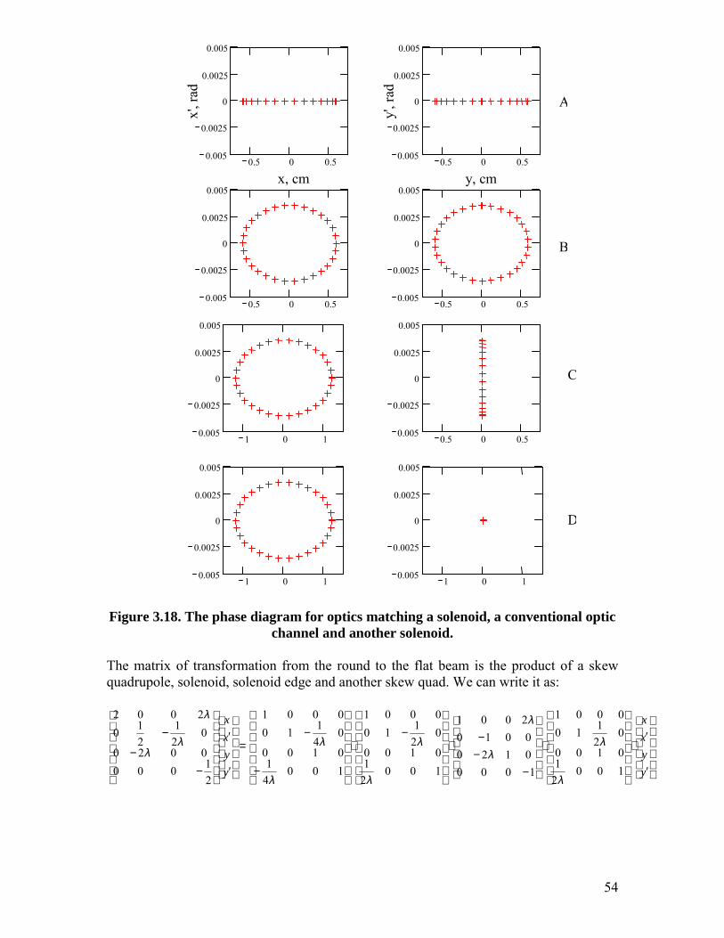
54

Figure 3.18. The phase diagram for optics matching a solenoid, a conventional opticchannel and another solenoid.

The matrix of transformation from the round to the flat beam is the product of a skewquadrupole, solenoid, solenoid edge and another skew quad. We can write it as:

′

′⋅

⋅

−−−

⋅

−

⋅

−

−=

′

′

−−

−

yyxx

yyxx

10021

0100

02110

0001

100001200010

2001

10021

0100

02110

0001

10041

0100

04110

0001

21000

0020

021

210

2002

λ

λλ

λ

λ

λ

λ

λλ

λ

λ

0.005

0.0025

0

0.0025

0.005

0.5 0 0.50.005

0.0025

0

0.0025

0.005

1 0 10.005

0.0025

0

0.0025

0.005

0.5 0 0.50.005

0.0025

0

0.0025

0.005

1 0 10.005

0.0025

0

0.0025

0.005

1 0 10.005

0.0025

0.0025

0.005

0

y', r

ad

x, cm y, cmx'

, rad

0.5 0 0.50.005

0.0025

0

0.0025

0.005

0.5 0 0.50.005

0.0025

0

0.0025

0.005

0.5 0 0.5

A

B

D

C

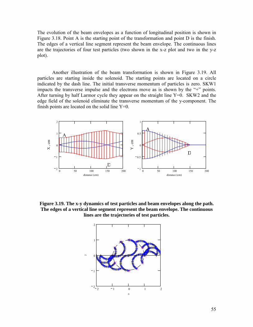
55

The evolution of the beam envelopes as a function of longitudinal position is shown inFigure 3.18. Point A is the starting point of the transformation and point D is the finish.The edges of a vertical line segment represent the beam envelope. The continuous linesare the trajectories of four test particles (two shown in the x-z plot and two in the y-zplot).

Another illustration of the beam transformation is shown in Figure 3.19. Allparticles are starting inside the solenoid. The starting points are located on a circleindicated by the dash line. The initial transverse momentum of particles is zero. SKW1impacts the transverse impulse and the electrons move as is shown by the “+” points.After turning by half Larmor cycle they appear on the straight line Y=0. SKW2 and theedge field of the solenoid eliminate the transverse momentum of the y-component. Thefinish points are located on the solid line Y=0.

Figure 3.19. The x-y dynamics of test particles and beam envelopes along the path.The edges of a vertical line segment represent the beam envelope. The continuous

lines are the trajectories of test particles.

0 50 100 150 2002

1

0

1

2

distance (cm)

X ,

cm

0 50 100 150 2001

0.5

0

0.5

1

distance (cm)

Y ,

cm

A

D

D

A

2 1 0 1 22

1

0

1

2

x

y .

56

Figure 3.20. The illustration of conversion of round beam into a flat beam.

The calculation above was done assuming a zero initial emittance (no thermal,space charge or similar emittances included.) Next we include the effect of an additionalemittance, as shown in Figure 3.21. A small value of noise is added to the transversemomentum in various places of the system in Figure 3.21. The noise has a normaldistribution. The first phase space diagram in Figure 3.21. shows the influence of themomentum spread in the injector (A, D, E). According to Equation 2, a transversetemperature of 0.2 eV (∆p/p≈1.8⋅10-4) at the injector (point A) leads to an increase in thetransverse momentum of particle into the main solenoid of ∆p2/p ≈9⋅10-5. A noise level of∆p/p =1.8⋅10-4 after SKW2 (point D) leads to a transverse momentum into the mainsolenoid of ∆p2/p =1.6⋅10-4 . This result illustrates the restriction on the emittance growthin the electron beam transport system. Consider that at point D the beam size in onedimension is very small. Since it is essential to transport a bunch containing a largenumber of electrons, the space-charge dominated bunch may acquire an additionalemittance due to the nonlinear part of the electric field. Another cause for increase intransverse momentum is RF induced transverse kick by the exit from an acceleratingcavity.

Figure 3.21. The influence of emittance growth along the transport channel on theresulting momentum spread sent to the main solenoid. The left and right diagrams

deal with the additional transverse momentum spread into the injector (A) andbefore accelerating (D), respectively . The magnitude of the noise is ∆∆∆∆p/p =1.8⋅⋅⋅⋅10-4

for both cases.

3.7.2. Injection of round electron beam generated by a magnetized cathode

It is possible to realize a non-destructive injection of an electron beam into themagnetic field of the solenoid if one can prepare the vortex like state of the electron beamwith the azimuth component of momentum of the particles proportional to the distancefrom the axis. In this case, the edge field of the solenoid may cancel the azimuthal

F F

5 .10 4 0 5 .10 40.001

5 .10 4

0

5 .10 4

0.001

.

4 .10 4 2 .10 4 0 2 .10 4 4 .10 44 .10 4

2 .10 4

0

2 .10 4

4 .10 4

.

σx' =σy' =9⋅10-5

y', r

ad

F

x', rad

y', r

ad

σx' =0, σy' =1.6⋅10-4

x', rad

F

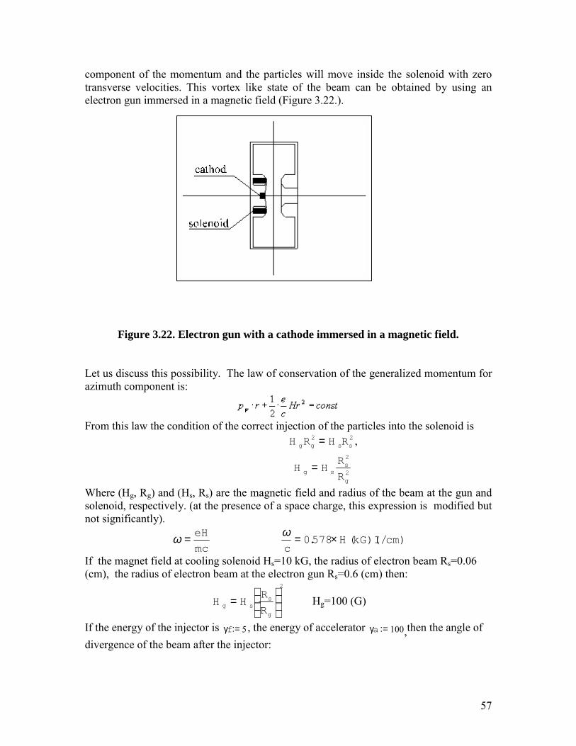
57

component of the momentum and the particles will move inside the solenoid with zerotransverse velocities. This vortex like state of the beam can be obtained by using anelectron gun immersed in a magnetic field (Figure 3.22.).

Figure 3.22. Electron gun with a cathode immersed in a magnetic field.

Let us discuss this possibility. The law of conservation of the generalized momentum forazimuth component is:

From this law the condition of the correct injection of the particles into the solenoid is22ssgg RHRH = ,

2

2

g

ssg R

RHH =

Where (Hg, Rg) and (Hs, Rs) are the magnetic field and radius of the beam at the gun andsolenoid, respectively. (at the presence of a space charge, this expression is modified butnot significantly).

mc

eH=ω

)/1)((578.0 cmkGHc

×=ω

If the magnet field at cooling solenoid Hs=10 kG, the radius of electron beam Rs=0.06(cm), the radius of electron beam at the electron gun Rs=0.6 (cm) then:

2

=

g

ssgR

RHH Hg=100 (G)

If the energy of the injector is γf 5:= , the energy of accelerator γa 100:= ,then the angle ofdivergence of the beam after the injector:

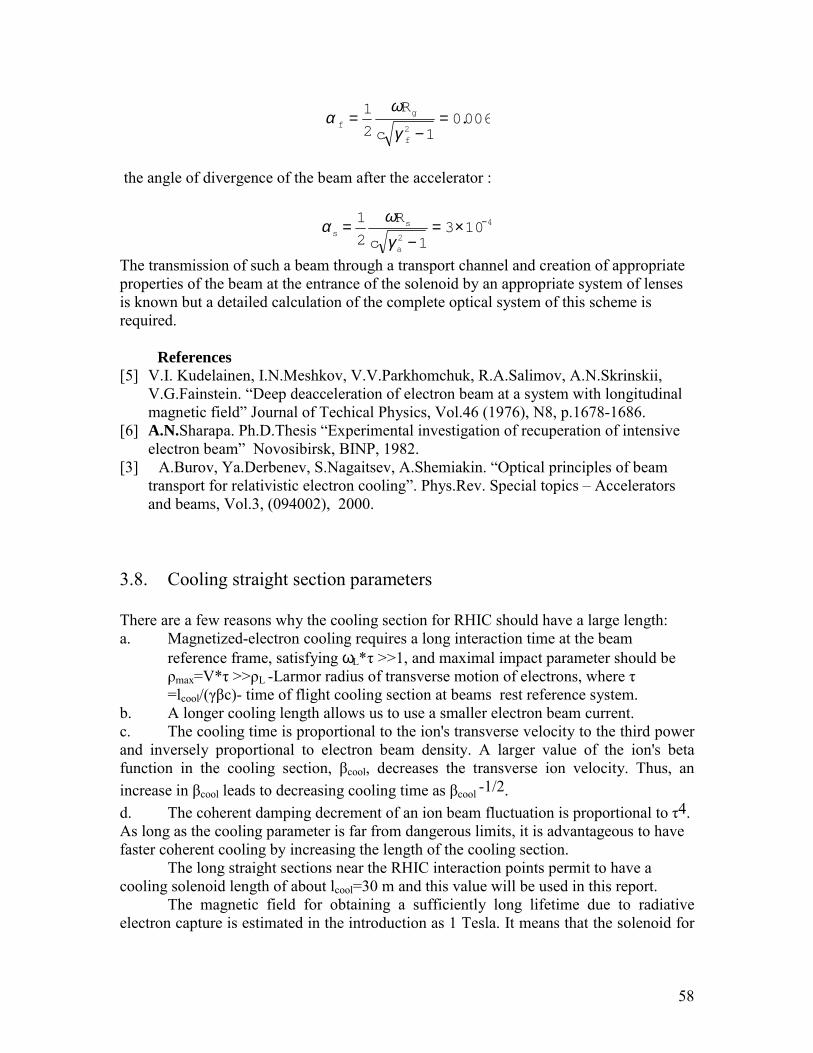
58

006.012

12

=−

=f

gf

c

R

γ

ωα

the angle of divergence of the beam after the accelerator :

4

2103

12

1 −×=−

=a

ss

c

R

γωα

The transmission of such a beam through a transport channel and creation of appropriateproperties of the beam at the entrance of the solenoid by an appropriate system of lensesis known but a detailed calculation of the complete optical system of this scheme isrequired.

References[5] V.I. Kudelainen, I.N.Meshkov, V.V.Parkhomchuk, R.A.Salimov, A.N.Skrinskii,

V.G.Fainstein. “Deep deacceleration of electron beam at a system with longitudinalmagnetic field” Journal of Techical Physics, Vol.46 (1976), N8, p.1678-1686.

[6] A.N.Sharapa. Ph.D.Thesis “Experimental investigation of recuperation of intensiveelectron beam” Novosibirsk, BINP, 1982.

[3] A.Burov, Ya.Derbenev, S.Nagaitsev, A.Shemiakin. “Optical principles of beamtransport for relativistic electron cooling”. Phys.Rev. Special topics – Acceleratorsand beams, Vol.3, (094002), 2000.

3.8. Cooling straight section parameters

There are a few reasons why the cooling section for RHIC should have a large length:a. Magnetized-electron cooling requires a long interaction time at the beam

reference frame, satisfying ωL*τ >>1, and maximal impact parameter should beρmax=V*τ >>ρL -Larmor radius of transverse motion of electrons, where τ=lcool/(γβc)- time of flight cooling section at beams rest reference system.

b. A longer cooling length allows us to use a smaller electron beam current.c. The cooling time is proportional to the ion's transverse velocity to the third powerand inversely proportional to electron beam density. A larger value of the ion's betafunction in the cooling section, βcool, decreases the transverse ion velocity. Thus, anincrease in βcool leads to decreasing cooling time as βcool -1/2.d. The coherent damping decrement of an ion beam fluctuation is proportional to τ4.As long as the cooling parameter is far from dangerous limits, it is advantageous to havefaster coherent cooling by increasing the length of the cooling section.

The long straight sections near the RHIC interaction points permit to have acooling solenoid length of about lcool=30 m and this value will be used in this report.

The magnetic field for obtaining a sufficiently long lifetime due to radiativeelectron capture is estimated in the introduction as 1 Tesla. It means that the solenoid for

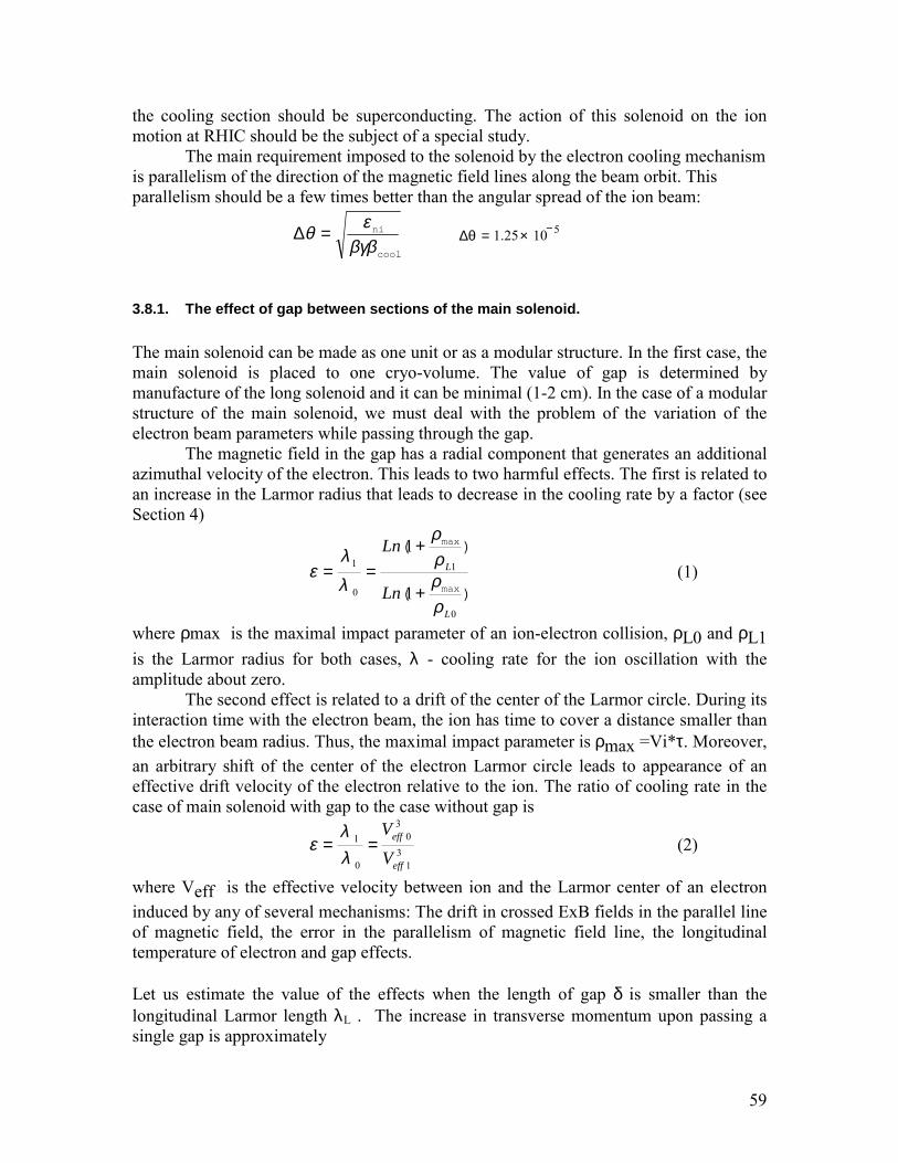
59

the cooling section should be superconducting. The action of this solenoid on the ionmotion at RHIC should be the subject of a special study.

The main requirement imposed to the solenoid by the electron cooling mechanismis parallelism of the direction of the magnetic field lines along the beam orbit. Thisparallelism should be a few times better than the angular spread of the ion beam:

cool

ni

βγβεθ =∆

∆θ 1.25 10 5−×=

3.8.1. The effect of gap between sections of the main solenoid.

The main solenoid can be made as one unit or as a modular structure. In the first case, themain solenoid is placed to one cryo-volume. The value of gap is determined bymanufacture of the long solenoid and it can be minimal (1-2 cm). In the case of a modularstructure of the main solenoid, we must deal with the problem of the variation of theelectron beam parameters while passing through the gap.

The magnetic field in the gap has a radial component that generates an additionalazimuthal velocity of the electron. This leads to two harmful effects. The first is related toan increase in the Larmor radius that leads to decrease in the cooling rate by a factor (seeSection 4)

)(

)(

max

max

0

1

0

1

1

1

L

L

Ln

Ln

ρρρρ

λλ

ε+

+== (1)

where ρmax is the maximal impact parameter of an ion-electron collision, ρL0 and ρL1is the Larmor radius for both cases, λ - cooling rate for the ion oscillation with theamplitude about zero.

The second effect is related to a drift of the center of the Larmor circle. During itsinteraction time with the electron beam, the ion has time to cover a distance smaller thanthe electron beam radius. Thus, the maximal impact parameter is ρmax =Vi*τ. Moreover,an arbitrary shift of the center of the electron Larmor circle leads to appearance of aneffective drift velocity of the electron relative to the ion. The ratio of cooling rate in thecase of main solenoid with gap to the case without gap is

31

30

0

1

eff

eff

VV

==λλ

ε (2)

where Veff is the effective velocity between ion and the Larmor center of an electroninduced by any of several mechanisms: The drift in crossed ExB fields in the parallel lineof magnetic field, the error in the parallelism of magnetic field line, the longitudinaltemperature of electron and gap effects.

Let us estimate the value of the effects when the length of gap δ is smaller than thelongitudinal Larmor length λL . The increase in transverse momentum upon passing asingle gap is approximately

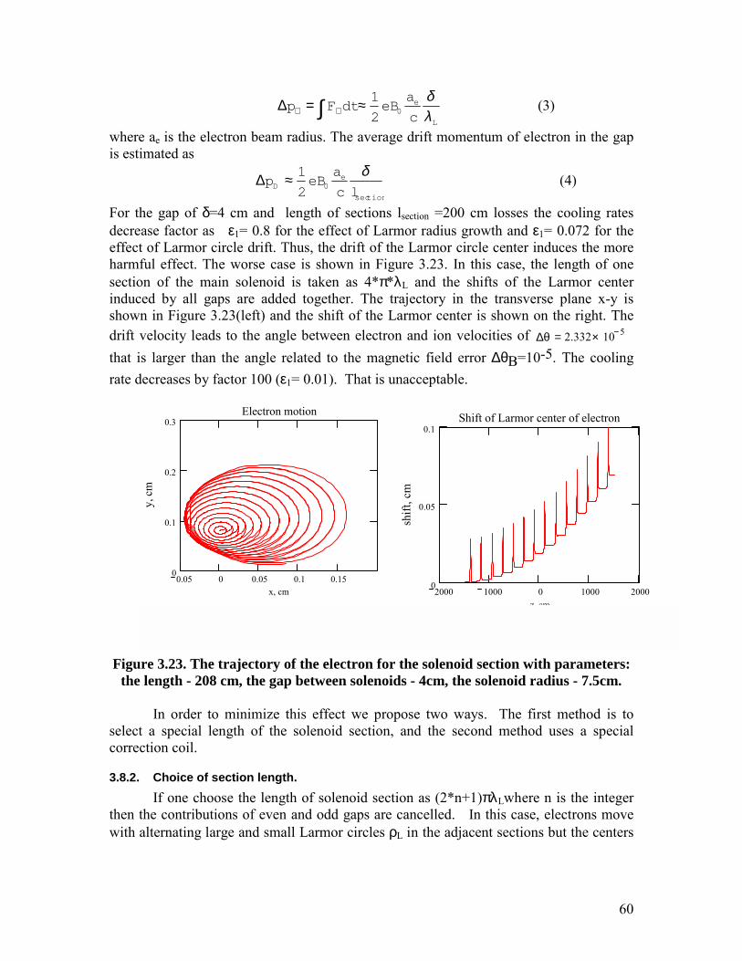
60

L

e

c

aeBdtFp

λδ

02

1≈=∆ ∫ ⊥⊥ (3)

where ae is the electron beam radius. The average drift momentum of electron in the gapis estimated as

tion

eD

lc

aeBp

sec

02

1 δ≈∆ (4)

For the gap of δ=4 cm and length of sections lsection =200 cm losses the cooling ratesdecrease factor as ε1= 0.8 for the effect of Larmor radius growth and ε1= 0.072 for theeffect of Larmor circle drift. Thus, the drift of the Larmor circle center induces the moreharmful effect. The worse case is shown in Figure 3.23. In this case, the length of onesection of the main solenoid is taken as 4*π*λL and the shifts of the Larmor centerinduced by all gaps are added together. The trajectory in the transverse plane x-y isshown in Figure 3.23(left) and the shift of the Larmor center is shown on the right. Thedrift velocity leads to the angle between electron and ion velocities of ∆θ 2.332 10 5−×=

that is larger than the angle related to the magnetic field error ∆θB=10-5. The coolingrate decreases by factor 100 (ε1= 0.01). That is unacceptable.

Figure 3.23. The trajectory of the electron for the solenoid section with parameters:the length - 208 cm, the gap between solenoids - 4cm, the solenoid radius - 7.5cm.

In order to minimize this effect we propose two ways. The first method is toselect a special length of the solenoid section, and the second method uses a specialcorrection coil.

3.8.2. Choice of section length.If one choose the length of solenoid section as (2*n+1)πλLwhere n is the integer

then the contributions of even and odd gaps are cancelled. In this case, electrons movewith alternating large and small Larmor circles ρL in the adjacent sections but the centers

2000 1000 0 1000 20000

0.05

0.1Shift of Larmor center of electron

z, cm

shift

, cm

0.05 0 0.05 0.1 0.150

0.1

0.2

0.3Electron motion

x, cm

y, c

m

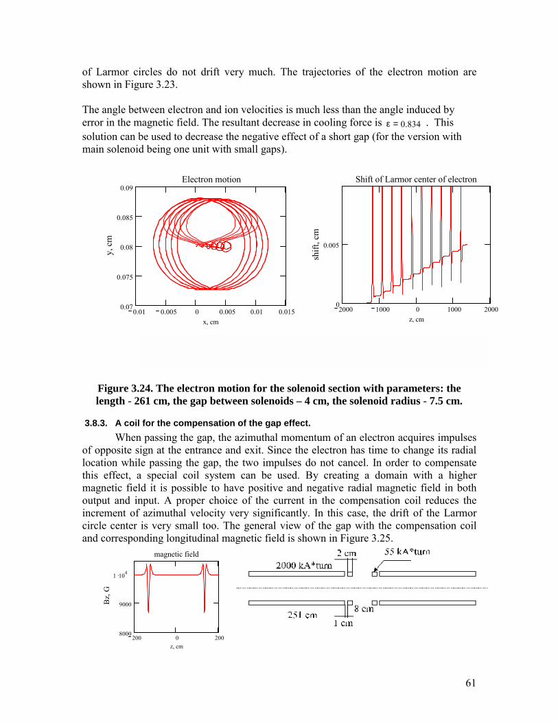
61

of Larmor circles do not drift very much. The trajectories of the electron motion areshown in Figure 3.23.

The angle between electron and ion velocities is much less than the angle induced byerror in the magnetic field. The resultant decrease in cooling force is ε 0.834= . Thissolution can be used to decrease the negative effect of a short gap (for the version withmain solenoid being one unit with small gaps).

Figure 3.24. The electron motion for the solenoid section with parameters: thelength - 261 cm, the gap between solenoids – 4 cm, the solenoid radius - 7.5 cm.

3.8.3. A coil for the compensation of the gap effect.When passing the gap, the azimuthal momentum of an electron acquires impulses

of opposite sign at the entrance and exit. Since the electron has time to change its radiallocation while passing the gap, the two impulses do not cancel. In order to compensatethis effect, a special coil system can be used. By creating a domain with a highermagnetic field it is possible to have positive and negative radial magnetic field in bothoutput and input. A proper choice of the current in the compensation coil reduces theincrement of azimuthal velocity very significantly. In this case, the drift of the Larmorcircle center is very small too. The general view of the gap with the compensation coiland corresponding longitudinal magnetic field is shown in Figure 3.25.

0.01 0.005 0 0.005 0.01 0.0150.07

0.075

0.08

0.085

0.09Electron motion

x, cm

y, c

m

2000 1000 0 1000 20000

0.005

Shift of Larmor center of electron

z, cmsh

ift, c

m

200 0 2008000

9000

1 .104

magnetic field

z, cm

Bz,

G

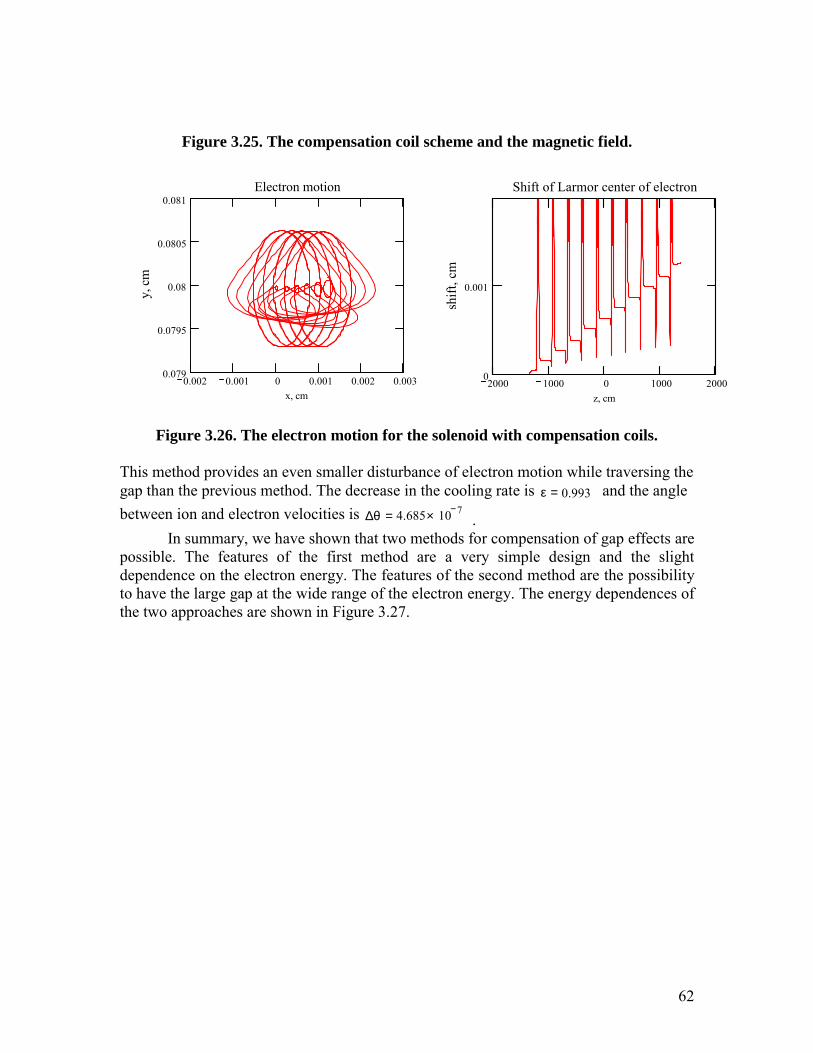
62

Figure 3.25. The compensation coil scheme and the magnetic field.

Figure 3.26. The electron motion for the solenoid with compensation coils.

This method provides an even smaller disturbance of electron motion while traversing thegap than the previous method. The decrease in the cooling rate is ε 0.993= and the anglebetween ion and electron velocities is ∆θ 4.685 10 7−×= .

In summary, we have shown that two methods for compensation of gap effects arepossible. The features of the first method are a very simple design and the slightdependence on the electron energy. The features of the second method are the possibilityto have the large gap at the wide range of the electron energy. The energy dependences ofthe two approaches are shown in Figure 3.27.

2000 1000 0 1000 20000

0.001

Shift of Larmor center of electron

z, cm

shift

, cm

0.002 0.001 0 0.001 0.002 0.0030.079

0.0795

0.08

0.0805

0.081Electron motion

x, cm

y, c

m

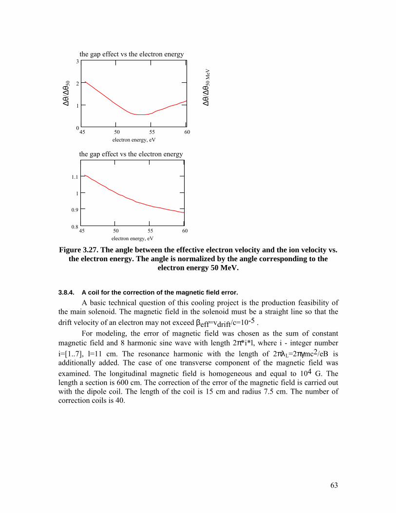
63

45 50 55 600

1

2

3the gap effect vs the electron energy

electron energy, eV

45 50 55 600.8

0.9

1

1.1

the gap effect vs the electron energy

electron energy, eV

Figure 3.27. The angle between the effective electron velocity and the ion velocity vs.the electron energy. The angle is normalized by the angle corresponding to the

electron energy 50 MeV.

3.8.4. A coil for the correction of the magnetic field error.A basic technical question of this cooling project is the production feasibility of

the main solenoid. The magnetic field in the solenoid must be a straight line so that thedrift velocity of an electron may not exceed βeff=vdrift/c=10-5 .

For modeling, the error of magnetic field was chosen as the sum of constantmagnetic field and 8 harmonic sine wave with length 2π*i*l, where i - integer numberi=[1..7], l=11 cm. The resonance harmonic with the length of 2πλL=2πγmc2/eB isadditionally added. The case of one transverse component of the magnetic field wasexamined. The longitudinal magnetic field is homogeneous and equal to 104 G. Thelength a section is 600 cm. The correction of the error of the magnetic field is carried outwith the dipole coil. The length of the coil is 15 cm and radius 7.5 cm. The number ofcorrection coils is 40.

∆θ/∆

θ 50

∆θ/∆

θ 50

MeV

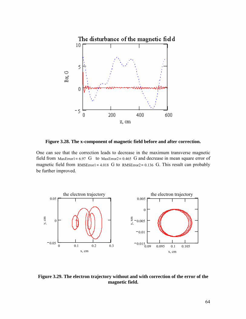
64

Figure 3.28. The x-component of magnetic field before and after correction.

One can see that the correction leads to decrease in the maximum transverse magneticfield from MaxError1 6.97= G to MaxError2 0.465= G and decrease in mean square error ofmagnetic field from RMSError1 4.018= G to RMSError2 0.136= G. This result can probablybe further improved.

Figure 3.29. The electron trajectory without and with correction of the error of themagnetic field.

0.09 0.095 0.1 0.1050.015

0.01

0.005

0

0.005the electron trajectory

x, cm

y, x

m

0 0.1 0.2 0.30.05

0

0.05the electron trajectory

x, cm

y, c

m

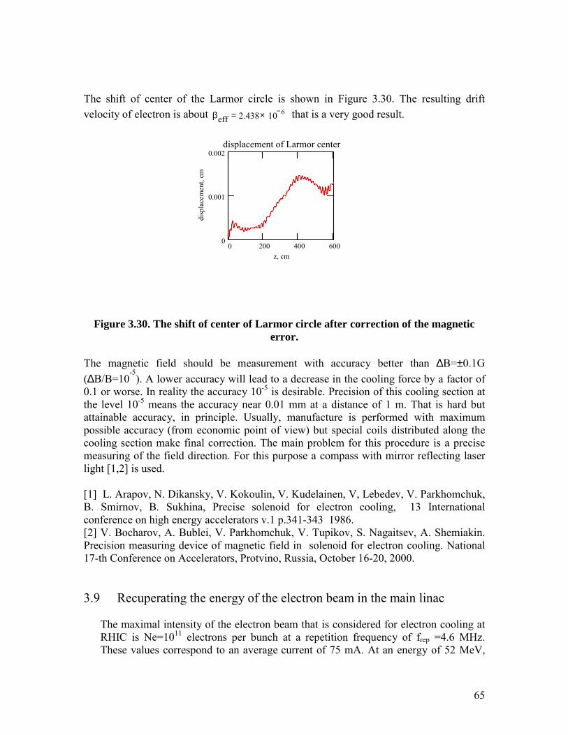
65

The shift of center of the Larmor circle is shown in Figure 3.30. The resulting driftvelocity of electron is about βeff 2.438 10 6−×= that is a very good result.

Figure 3.30. The shift of center of Larmor circle after correction of the magneticerror.

The magnetic field should be measurement with accuracy better than ∆B=±0.1G(∆B/B=10

-5). A lower accuracy will lead to a decrease in the cooling force by a factor of

0.1 or worse. In reality the accuracy 10-5 is desirable. Precision of this cooling section atthe level 10-5 means the accuracy near 0.01 mm at a distance of 1 m. That is hard butattainable accuracy, in principle. Usually, manufacture is performed with maximumpossible accuracy (from economic point of view) but special coils distributed along thecooling section make final correction. The main problem for this procedure is a precisemeasuring of the field direction. For this purpose a compass with mirror reflecting laserlight [1,2] is used.

[1] L. Arapov, N. Dikansky, V. Kokoulin, V. Kudelainen, V, Lebedev, V. Parkhomchuk,B. Smirnov, B. Sukhina, Precise solenoid for electron cooling, 13 Internationalconference on high energy accelerators v.1 p.341-343 1986.[2] V. Bocharov, A. Bublei, V. Parkhomchuk, V. Tupikov, S. Nagaitsev, A. Shemiakin.Precision measuring device of magnetic field in solenoid for electron cooling. National17-th Conference on Accelerators, Protvino, Russia, October 16-20, 2000.

3.9 Recuperating the energy of the electron beam in the main linac

The maximal intensity of the electron beam that is considered for electron cooling atRHIC is Ne=1011 electrons per bunch at a repetition frequency of frep =4.6 MHz.These values correspond to an average current of 75 mA. At an energy of 52 MeV,

0 200 400 6000

0.001

0.002displacement of Larmor center

z, cm

disp

lace

men

t, cm

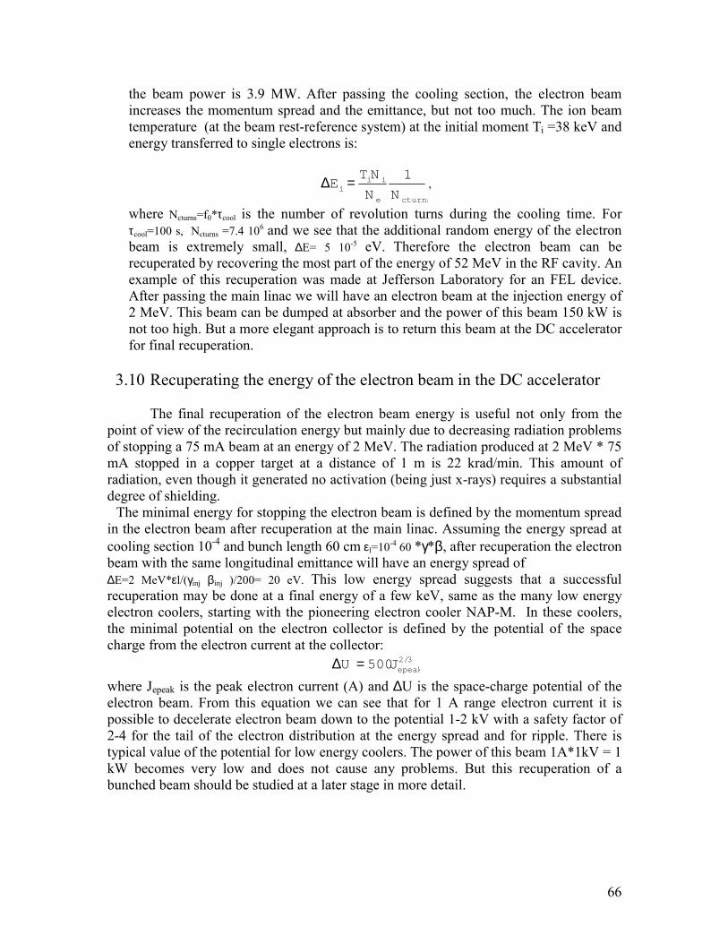
66

the beam power is 3.9 MW. After passing the cooling section, the electron beamincreases the momentum spread and the emittance, but not too much. The ion beamtemperature (at the beam rest-reference system) at the initial moment Ti =38 keV andenergy transferred to single electrons is:

cturnse

iii

NN

NTE

1=∆ ,

where Ncturns=f0*τcool is the number of revolution turns during the cooling time. Forτcool=100 s, Ncturns =7.4 106 and we see that the additional random energy of the electronbeam is extremely small, ∆E= 5 10-5 eV. Therefore the electron beam can berecuperated by recovering the most part of the energy of 52 MeV in the RF cavity. Anexample of this recuperation was made at Jefferson Laboratory for an FEL device.After passing the main linac we will have an electron beam at the injection energy of2 MeV. This beam can be dumped at absorber and the power of this beam 150 kW isnot too high. But a more elegant approach is to return this beam at the DC acceleratorfor final recuperation.

3.10 Recuperating the energy of the electron beam in the DC accelerator

The final recuperation of the electron beam energy is useful not only from thepoint of view of the recirculation energy but mainly due to decreasing radiation problemsof stopping a 75 mA beam at an energy of 2 MeV. The radiation produced at 2 MeV * 75mA stopped in a copper target at a distance of 1 m is 22 krad/min. This amount ofradiation, even though it generated no activation (being just x-rays) requires a substantialdegree of shielding. The minimal energy for stopping the electron beam is defined by the momentum spreadin the electron beam after recuperation at the main linac. Assuming the energy spread atcooling section 10-4 and bunch length 60 cm εl=10-4 60 *γ*β, after recuperation the electronbeam with the same longitudinal emittance will have an energy spread of∆E=2 MeV*εl/(γinj βinj )/200= 20 eV. This low energy spread suggests that a successfulrecuperation may be done at a final energy of a few keV, same as the many low energyelectron coolers, starting with the pioneering electron cooler NAP-M. In these coolers,the minimal potential on the electron collector is defined by the potential of the spacecharge from the electron current at the collector:

3/2500 epeakJU =∆where Jepeak is the peak electron current (A) and ∆U is the space-charge potential of theelectron beam. From this equation we can see that for 1 A range electron current it ispossible to decelerate electron beam down to the potential 1-2 kV with a safety factor of2-4 for the tail of the electron distribution at the energy spread and for ripple. There istypical value of the potential for low energy coolers. The power of this beam 1A*1kV = 1kW becomes very low and does not cause any problems. But this recuperation of abunched beam should be studied at a later stage in more detail.

67

4. KEY-PHYSICAL PROCESSESFundamentals of electron cooling theory

4.1 The drag force in the absence of a magnetic field

The electric field produced by ions moving in an electron gas causes a perturbation of theelectrons by imparting a fraction of the ion’s energy of motion to them. In moving pathan electron with an impact parameter ρ at a velocity V, a particle with a charge Zietransfers to the electron a momentum

V

eZp i

ρ

22=∆ ⊥ (1)

The momentum transfer is enhanced in close collisions, and for the minimal impactparameter

2)/( cV

rZ ei=ρ (2)

where re is the classical electron radius, the transferred momentum reaches its largestpossible value 2mV, where m is the mass of the electron. Various effects may limit themaximal impact parameter. In the case of a high-density electron beam, the electronmotion has to be taken into account. If the time τi =ρ/V it takes the particle to pass by theelectron approaches the time for which the Debye shielding is established owing toplasma oscillations with a frequency eee rnc πω 4= , the interaction efficiency is reducedfor ρ>ρmax =V/ωe. For an electron beam that is not too dense, the time of flight throughthe cooling section τflight (at beam reference system) limits the interaction time τi <τflightand as result, the impact parameter is bound by ρmax =Vτflight (Provided that ωe<1/τflight ).For the range of allowed impact parameters ρmin <ρ<ρmax , it is easy to calculate the meanenergy loss of a particle moving in an electron gas:

∫ −=∆−= ⊥max

min

422

22

ρ

ρ

ρπρVm

LnneZdVn

m

p

dt

dE

e

ceie

e

(3)

where the Coulomb logarithm

)ln(min

max

ρρ=cLn

and thus we obtain the drag force (defined through the energy loss by FV=dE/dt) [1]:

VVm

LnneZF

e

cei3

42

−= (4)

If it is necessary to take into account the proper thermal motion of electrons in a beam,the drag force is averaged over the velocity distribution fe (Ve ). Such integrals are most

68

readily computed by applying the Coulomb analog of force in velocity space (neglectingthe change in the Coulomb logarithm Lnc ). Assume the velocity distribution of electrons to have the shape of a flat disk with atransverse radius Ve⊥ and longitudinal width Ve|| , and consider Ve|| << Ve⊥ . In this case,longitudinal drag force takes the form

>>+

−

<−=

⊥

⊥||||22

||

||

||

||

||||||

||

2

42

||8

e

e

ee

ee

cei

VVVV

VVV

VVVV

VmLnneZF π

(5)

At ion velocity V|| <Ve|| within the electron distribution, the longitudinal drag forceincreases linearly; in the region Ve|| <V|| <Ve⊥ it falls weakly, and when V||>Ve⊥ , itdecreases rapidly (in proportion to V-2). The transverse drag force in the case V⊥ <Ve⊥

F∝ V⊥ /Ve⊥3 is seen to fall rapidly (in proportion to Ve⊥

-3) at high electron beamtemperature, and the possibility of attaining high cooling rate is limited by the fast motionof electrons (with velocity Ve⊥ >>V).

4.2 The drag force in a magnetic field

The longitudinal magnetic field B accompanying the electron beam in the cooling zonealters the drag force significantly. The reason for such a phenomenon is that owing to thethermal motion, the Larmor radius of the electron spiral movement

eB

cVm eeL

⊥=ρ may be significantly smaller then the maximum impact parameter

ρL<<ρmax . The transverse thermal motion of electrons in the “magnetized” zone ofimpact parameters exerts an influence on the ions-electrons interaction kinetics, while thecontribution of electrons from this region of impact parameters to the drag force increasesstrongly and becomes predominant. The next figure shows the change in momentum of aproton passing by an electron at a distance ρ in case of magnetic fields B being equal to0,100,1000G. This result was calculated by direct computer simulation of electron-ioninteraction. The single charge of ion (proton) moves transversely to magnetic fielddirection with velocity 3 106 cm/s. Multiplication of the change in proton momentum byρ2 permits the more correct comparison of contributions of different impact parameters tothe total drag force with due regard for the change in number of electrons present in thevolume element ne Vτflight 2πρ dρ:

69

ρρπρ d

VnpF e 2)( 2∫ ∆= . The constancy of the product ∆pρ2 within the range of impact

parameters (ρ1,ρ2) indicates that contribution of this region of impact parameters to the

drag force is )ln(2)(1

22

ρρπρ Vnp e∆

10-5 10-4 10-3 10-2 10-1

0

2

4

6

8

10

12

B=1000 G è Ve=107 cm/s

B=1000 G

B=100 G

B=0

∆ pρ2 , 1

0-30g cm3s-1

ρ, ρ, ρ, ρ, (cm)

Figure 4.1. Contribution of collisions with electrons to drag force versus the impactparameter in the case of motion transverse to magnetic field. The momentum

transverse for an electron beam of zero temperature are shown for various magneticfields, as well as the influence of the transverse electron velocity at B=1000 G (curve

marked by squares). The proton velocity V=3 106 cm/s, the interaction time withelectron beam ττττflight =4 10-8 s.

From Figure 4.1. one can see that in the case of collision with electrons at rest (withouttheir proper thermal motion), the magnetic field suppresses by a factor of two the energytransverse at impact parameters exceeding V/ωL (ωL=eB/mec). This is because theelectrons are capable of free motion only along the magnetic field lines and the averagingof energy transfers over the electrons location at identical distances ρ from the iontrajectory, but with different azimuthal angles, suppresses the transfer of energy fromproton to an electron in proportion to <cos2(φ)> , where φ is the angle between themomentum transferred from the proton and magnet field line. When electrons have a

70

noticeable velocity owing to transverse temperature in the region of small impactparameters (ρ<<Ve⊥ /ωL), where the action of magnetic field is insignificant, the energytransfer becomes small:

3

422 2

⊥

=∆ee

i

Vm

eZpρ and for the parameters in the calculated example, the force is only 10-31

gcm3/s. But for large impact ρ>ρL=V/ωL=5.6 10-4 cm, the contribution increases up to2*10-30 g cm2 s, that is close to the contribution for the electron beam with zerotemperature. The magnetic field maintains a large energy transfer within the range ofimpact parameters from 5 10-4 up to 3 10-2 cm (ρL--ρmax). As a result, the drag force forsmall proton velocities (V<<Ve⊥ ) in the presence of a magnetic field turns out to be manytimes higher than that without the magnetic field, and it depends weakly (ln(ρmax/ρL)) onthe velocity of transverse electron motion instead of falling as (Ve⊥ )-3. For the description of the drag force in real experiments, it is convenient to have ananalytical expression that allows for numerical computation for comparison withexperimental results. Reflection on this issue have resulted in a drag force determined bythe formula [2]:

)ln()(

4

min

minmax

322

42

ρρρρρ

+++

+−=

L

L

effe

ei

VVm

VneZF

!!

(6)

and the cooling rate at the beam-reference system is:

)ln()/(

4)ln(

)(

4

min

minmax

322min

minmax

322

42

ρρρρρ

ρρρρρλ

+++

+=

+++

+=−=

L

L

eff

eie

L

L

effie

ei

i cVV

cnrr

VVMm

neZ

VM

F

(7),where Veff –is the effective velocity of motion of the Larmor circles related both to thelongitudinal electron velocity and transverse drift motion caused by the magnetic andelectric fields owing to the space charge of beams and inaccuracies in the creationconcomitant magnetic field at cooling section. The argument of logarithm makes it possible to extend the application of theseexpressions to parameter ranges that are clearly not logarithmic. Thus, at small velocityof motion, when ρmin =Zi e2 /me V>>ρmax =V/ωe >>ρL for the electron gas with zerotemperature (Veff=0), the drag force is assumed to have the form:

e

i

VneZF

ω24−= (8)

and force linearly increased up to its maximum as the ion velocity increases up to Vmax= c(4 π Z2

i r3e ne )1/6 , after which it drops in according to formula ( ) as V-2 . The maximal

cooling rate at this linear range of velocity is equal to:

πωπ

πλ e

i

i

p

e

e

e

i

ie

i A

Z

M

m

m

ne

M

Zm

VM

F ===2

max

4 (9),

and at this case the drag force and cooling rate increase with electron beam density inproportion to (ne)1/2 as was measured at MOSOL experiments.

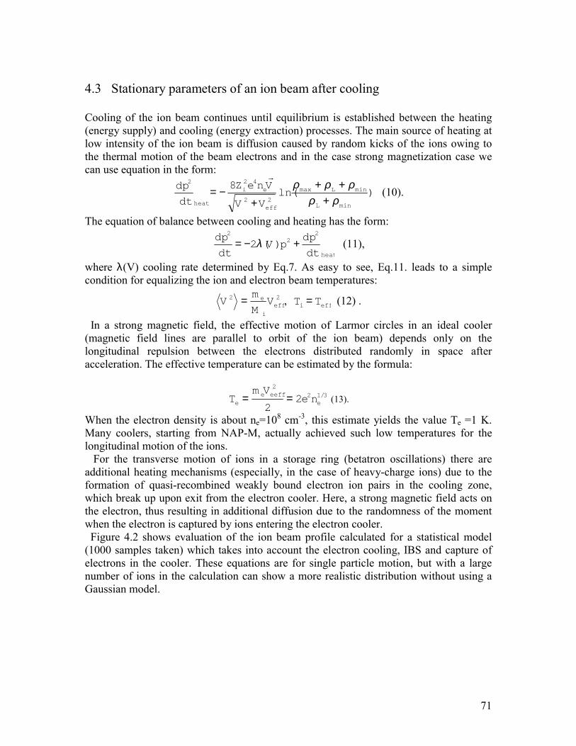
71

4.3 Stationary parameters of an ion beam after cooling

Cooling of the ion beam continues until equilibrium is established between the heating(energy supply) and cooling (energy extraction) processes. The main source of heating atlow intensity of the ion beam is diffusion caused by random kicks of the ions owing tothe thermal motion of the beam electrons and in the case strong magnetization case wecan use equation in the form:

)ln(8

min

minmax

22

422

ρρρρρ

+++

+−=

L

L

eff

ei

heat VV

VneZ

dt

dp!

(10).

The equation of balance between cooling and heating has the form:

heatdt

dppV

dt

dp 22

2

)(2 +−= λ (11),

where λ(V) cooling rate determined by Eq.7. As easy to see, Eq.11. leads to a simplecondition for equalizing the ion and electron beam temperatures:

22eff

i

e VM

mV = , effi TT = (12) .

In a strong magnetic field, the effective motion of Larmor circles in an ideal cooler(magnetic field lines are parallel to orbit of the ion beam) depends only on thelongitudinal repulsion between the electrons distributed randomly in space afteracceleration. The effective temperature can be estimated by the formula:

3/122

22

eeeffe

e neVm

T == (13).

When the electron density is about ne=108 cm-3, this estimate yields the value Te =1 K.Many coolers, starting from NAP-M, actually achieved such low temperatures for thelongitudinal motion of the ions. For the transverse motion of ions in a storage ring (betatron oscillations) there areadditional heating mechanisms (especially, in the case of heavy-charge ions) due to theformation of quasi-recombined weakly bound electron ion pairs in the cooling zone,which break up upon exit from the electron cooler. Here, a strong magnetic field acts onthe electron, thus resulting in additional diffusion due to the randomness of the momentwhen the electron is captured by ions entering the electron cooler. Figure 4.2 shows evaluation of the ion beam profile calculated for a statistical model(1000 samples taken) which takes into account the electron cooling, IBS and capture ofelectrons in the cooler. These equations are for single particle motion, but with a largenumber of ions in the calculation can show a more realistic distribution without using aGaussian model.

72

-0,1 0,0 0,1 0,2

1

10

100

0 0.1 h 0.2 h 0.3 h 0.5 h 0.6 h 0.7 h 0.8 h 0.9 h 1 hho

rizon

tal p

rofil

e

X (cm)

Figure 4.2. Transverse ion beam profiles (horizontal) in the cooling section. Theprofiles are shown at time intervals of 0.1 hour.

From this figure we can see first of all cooled ions with small amplitude. At center ofbeam we see at formation the cooled ion beam core just at the first stage of cooling. Theions with large amplitude cooled slowly and the tail of the distribution is drawn into thecooled core only in 1 hour. This code was written at Fortran and was verified on theexperimentally measured results from the electron cooling of high charge ions in the SIScooler.

4.4 The space charge tune shift (Laslett tune shift)

The strongest additional heating in the transverse direction is due to the influence ofmachine resonances. The field of the cooled ion beam space charge results in the shiftand spread of the frequencies of betatron oscillations, and the largest possible tune-shift∆νmax serves as a good characteristic. At the same time, the smallest transverseemittance achievable in cooling is limited by the value:

max32

2

min νγβπβσε

∆==

⊥

⊥

b

ii

l

RrN (14),

where lb is the ion bunch length, r=(Zie)2 /(Ai Mp) is the classical ion radius, β⊥ is the betafunction, and R the average radius of storage ring.

73

The experiments have revealed that the most typical tune shift, obtained underconditions of electron cooling amounts to ∆νmax=0.1-0.2. Usually, the ion beam sizedecreases until the tune shift reaches the value indicated and this results was obtained at NAP-Mexperiments with the proton beam and at SIS cooler with heavy ion beam (see ECOOL99 proceeding, page179, fig.7).

4.5 The Intra Beam Scattering

Ion scattering within the ion beam is a factor determining the longitudinal momentumspread in the beam for ion currents that are not too small. As a rule, the decrement of thelongitudinal electron cooling is significantly higher than the transverse one (the reason isflatness of the electron beam distributions in velocity space) and, consequently, thelongitudinal spread of ion momentum is significantly lower in the co-moving frame ofreference than the transverse momentum spread. At the beam reference system the IntraBeam Scattering can be described as relaxation in the ion gas. The time of this relaxationin the beams reference system can be written in the form:

32

42

2

)(411

VM

LnneZ

dt

pd

p i

ibsii

ibs

πτ

=∆∆

= (15)

where γβπε b

ii

l

Nn

⊥⊥

=2

is the ion beam density at beam system, Lnibs is the Coulomb

logarithm for IBS.As a result, for flat velocity distribution in the ion beam (in the beam reference system V||<<V⊥ ) the IBS leads to an enhancement of the longitudinal momentum spread at aheating rate:

b

ibsii

l

cLnNr

p

p

dt

d

⊥

=

∆

βεβγ 2/333

22

|| 2, (16)

where ⟨⟩ - mean averaging along the ring circumference. For example, this equationallows a comparison to HERA measurements from report M.-P. Zorzano, R.Wanzenberg, “Intrabeam scattering and the coasting beam in the HERA proton ring”,CERN-SL-2000-072 AP, fig.2 meas.3)0.5

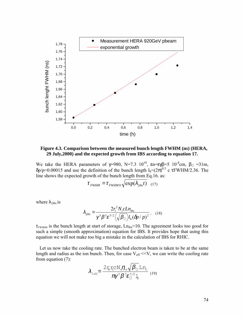
74

0,0 0,2 0,4 0,6 0,8 1,0 1,2 1,4

1,58

1,60

1,62

1,64

1,66

1,68

1,70

1,72

1,74

1,76

1,78 Measurement HERA 920GeV pbeam exponential growth

bunc

h le

nght

FW

HM

(ns)

time (h)

Figure 4.3. Comparison between the measured bunch length FWHM (ns) (HERA,29 July,2000) and the expected growth from IBS according to equation 17.

We take the HERA parameters of γ=980, N=7.3 1010, εn=εγβ=5 10-4cm, β⊥ =31m,δp/p=0.00015 and use the definition of the bunch length lb=(2π)0.5 c τFWHM/2.36. Theline shows the expected growth of the bunch length from Eq.16. as:

)exp( ||0 tibsFWHMFWHM λττ = (17)

where λ ||ibs is

22/333

2

||)/(

2ppl

cLnNr

b

ibsiiibs

δβεβγλ

⊥

= , (18)

τFWHM0 is the bunch length at start of storage, Lnibs=10. The agreement looks too good forsuch a simple (smooth approximation) equation for IBS. It provides hope that using thisequation we will not make too big a mistake in the calculation of IBS for RHIC.

Let us now take the cooling rate. The bunched electron beam is taken to be at the samelength and radius as the ion bunch. Then, for case Veff <<V, we can write the cooling ratefrom equation (7):

b

ceeielab

l

LncNrr2/535

2

⊥

⊥=εβπγ

βηλ (19)

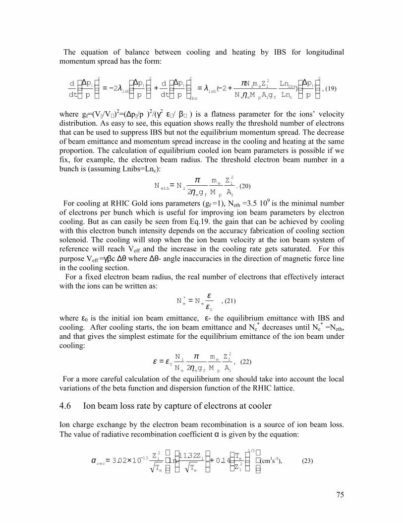
75

The equation of balance between cooling and heating by IBS for longitudinalmomentum spread has the form:

2

||22

||

2

||

2

|| )2(2

∆+−=

∆+

∆−=

∆p

p

Ln

Ln

gAMN

ZmN

p

p

dt

d

p

p

p

p

dt

d

c

ibs

fipee

ieilab

ibs

lab ηπλλ , (19)

where gf=(V||/V⊥ )2=(∆p||/p )2/(γ2 ε⊥ / β⊥ ) is a flatness parameter for the ions’ velocitydistribution. As easy to see, this equation shows really the threshold number of electronsthat can be used to suppress IBS but not the equilibrium momentum spread. The decreaseof beam emittance and momentum spread increase in the cooling and heating at the sameproportion. The calculation of equilibrium cooled ion beam parameters is possible if wefix, for example, the electron beam radius. The threshold electron beam number in abunch is (assuming Lnibs=Lnc):

i

i

p

e

fe

ieth A

Z

M

m

gNN

2

2ηπ= . (20)

For cooling at RHIC Gold ions parameters (gf =1), Neth =3.5 109 is the minimal numberof electrons per bunch which is useful for improving ion beam parameters by electroncooling. But as can easily be seen from Eq.19. the gain that can be achieved by coolingwith this electron bunch intensity depends on the accuracy fabrication of cooling sectionsolenoid. The cooling will stop when the ion beam velocity at the ion beam system ofreference will reach Veff and the increase in the cooling rate gets saturated. For thispurpose Veff =γβc ∆θ where ∆θ- angle inaccuracies in the direction of magnetic force linein the cooling section. For a fixed electron beam radius, the real number of electrons that effectively interactwith the ions can be written as:

0

*

εε

ee NN = , (21)

where ε0 is the initial ion beam emittance, ε- the equilibrium emittance with IBS andcooling. After cooling starts, the ion beam emittance and Ne

* decreases until Ne* =Neth,

and that gives the simplest estimate for the equilibrium emittance of the ion beam undercooling:

i

i

p

e

fee

i

A

Z

M

m

gN

N 2

0 2ηπεε = , (22)

For a more careful calculation of the equilibrium one should take into account the localvariations of the beta function and dispersion function of the RHIC lattice.

4.6 Ion beam loss rate by capture of electrons at cooler

Ion charge exchange by the electron beam recombination is a source of ion beam loss.The value of radiative recombination coefficient α is given by the equation:

+

×= −

3/1

2

213 14.0

32.11ln1002.3

i

e

e

i

e

irec Z

T

T

Z

T

Zα (cm3s-1), (23)

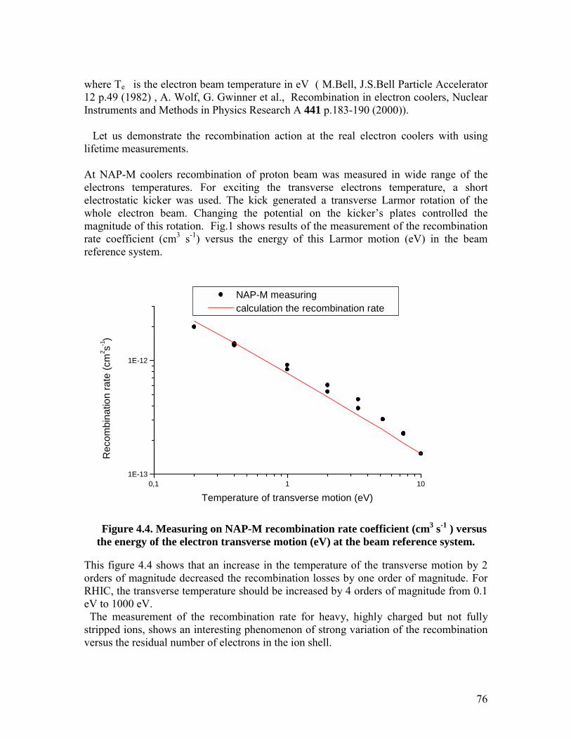
76

where Te is the electron beam temperature in eV ( M.Bell, J.S.Bell Particle Accelerator12 p.49 (1982) , A. Wolf, G. Gwinner et al., Recombination in electron coolers, NuclearInstruments and Methods in Physics Research A 441 p.183-190 (2000)).

Let us demonstrate the recombination action at the real electron coolers with usinglifetime measurements.

At NAP-M coolers recombination of proton beam was measured in wide range of theelectrons temperatures. For exciting the transverse electrons temperature, a shortelectrostatic kicker was used. The kick generated a transverse Larmor rotation of thewhole electron beam. Changing the potential on the kicker’s plates controlled themagnitude of this rotation. Fig.1 shows results of the measurement of the recombinationrate coefficient (cm3 s-1) versus the energy of this Larmor motion (eV) in the beamreference system.

0,1 1 101E-13

1E-12

NAP-M measuring calculation the recombination rate

Rec

ombi

natio

n ra

te (c

m2 s-1

)

Temperature of transverse motion (eV)

Figure 4.4. Measuring on NAP-M recombination rate coefficient (cm3 s-1 ) versusthe energy of the electron transverse motion (eV) at the beam reference system.

This figure 4.4 shows that an increase in the temperature of the transverse motion by 2orders of magnitude decreased the recombination losses by one order of magnitude. ForRHIC, the transverse temperature should be increased by 4 orders of magnitude from 0.1eV to 1000 eV. The measurement of the recombination rate for heavy, highly charged but not fullystripped ions, shows an interesting phenomenon of strong variation of the recombinationversus the residual number of electrons in the ion shell.

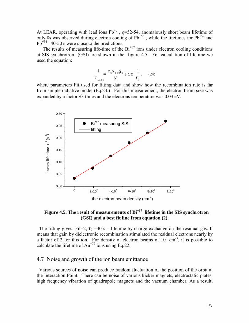
77

At LEAR, operating with lead ions Pb+q , q=52-54, anomalously short beam lifetime ofonly 8s was observed during electron cooling of Pb+53 , while the lifetimes for Pb+52 andPb+54 40-50 s were close to the predictions. The results of measuring life-time of the Bi+67 ions under electron cooling conditionsat SIS synchrotron (GSI) are shown in the figure 4.5. For calculation of lifetime weused the equation:

0

11

τγηα

τ+= Fit

n erece

life

, (24)

where parameters Fit used for fitting data and show how the recombination rate is farfrom simple radiative model (Eq.23.) . For this measurement, the electron beam size wasexpanded by a factor √3 times and the electrons temperature was 0.03 eV.

0 2x107 4x107 6x107 8x107 1x108

0,00

0,05

0,10

0,15

0,20

0,25

0,30

Bi+67 measuring SIS fitting

inve

rs li

fe ti

me

τ−1 ( s

−1)

the electron beam density (cm-3)

Figure 4.5. The result of measurements of Bi+67 lifetime in the SIS synchrotron(GSI) and a best fit line from equation (2).

The fitting gives: Fit=2, τ0 =30 s – lifetime by charge exchange on the residual gas. Itmeans that gain by dielectronic recombination stimulated the residual electrons nearly bya factor of 2 for this ion. For density of electron beams of 108 cm-3, it is possible tocalculate the lifetime of Au+79 ions using Eq.22.

4.7 Noise and growth of the ion beam emittance

Various sources of noise can produce random fluctuation of the position of the orbit atthe Interaction Point. There can be noise of various kicker magnets, electrostatic plates,high frequency vibration of quadrupole magnets and the vacuum chamber. As a result,

78

the ion bunch will receive a random kick at the IP with an amplitude proportional todeflection of the counter rotating bunch from central position x:

IP

ii

xx

βπξθ 2)( =∆ , (25)

where ξii =ri Ni /(4 π εn ) is the parameter of beam-beam interaction at single collision.This kick excites a coherent oscillation of the ion bunch for the decoherence time ofRHIC. During the decay, the coherent oscillation of the energy of this motion can bedamped by coherent interaction with cooling electron beam or with a standard feedbacksystem. Otherwise this energy passes on to the chaotic thermal motion of the ions. If weneglect the coherent damping, the heating rate of the beam emittance by this process is

22

0

)2(xnf

dt

d

IP

iiIP β

πξε = (26)

For the process of cooling, the increase in density of the ion beam and possible ξiiincrease reach an equilibrium state when cooling balances against this source of heating.The simulation code sicool.mcd takes into account this process. Time of decay ofcoherent oscillation after singe kick can be estimated (V. Lebedev, V. Parkhomchuk, V.Shiltsev, G. Stupakov, Emittance growth due to noise and its suppression with feedbacksystem in large hadron colliders, Particle Accelerators, V44, pp.147-264, 1994) as:

,2.0 iiIPn ξν ≈∆ ν∆= 1

turnsN (27)

When ξii =0.006, nIP =6 number of turns for decoherence ion bunch oscillation becomevery short Nturns =160. The coherent oscillation damping system should be powerful fordamping the oscillation in a very short time.

4.8 Requirement on impedance after cooling In low energy coolers when the transverse emittances and longitudinal momentumspread decreases by a few order magnitude as a result of cooling, the beam may becomeunstable. The “Keil-Schnell” threshold of ion beam current can be written in the form [3]

2

0

22 )/(

≤p

p

I

ecM

Z

AF

n

Z p

i

Ln δηγβ

, (28)

where FL ≈1 and I0=eZif0N is the average ion beam current for a coasting beam. For abunched beam, the local (peak) current can be used for a rough estimate, Ipeak=eZiβc/lb .For RHIC with Gold*Gold collision, I0= 60mA and Ipeak=5 A, the impedance is limited asZ/n<10 Ω and thus is not really a problem. The process of cooling should be controlledsuch that the transverse cooling (decreasing the ion beam emittance) would not producesimultaneously a large decrease of the longitudinally momentum spread. In this case, therequirement on the longitudinal coupling impedance after cooling is not higher thenwithout cooling. The question of coherent interaction of the ion bunch with coolingelectron beam will discussed at section 5.2.

79

[1] G.I. Budker, A.N. Skrinsky “Electron cooling” Uspekhi Fizicheskikh Nauk, v/124, 4p.561, 1978.[2] V.V. Parkhomchuk, A.N. Skrinsky “Elaectron cooling: 35 years of development”Physics-Uspekhi 43(5),pp. 433-452,2000[3] J.Bosser,. C.Carli, M.Chanel, N.Madsen, S.Maury, D.Mohl, G.Tranquille, “Stabillityof cooled beams”, ECOOL’99, Nuclear Instrum. And Methods in Physics Research A441(2000) pp.1-8

80

5. COLLECTIVE EFFECTS5.1 Laslett tune shift

The collective space charge field manifested itself in low energy coolers by a halt of thecooling taking place when the tune shift becomes larger than 0.01-0.1. The value of theLaslett tune-shift can be written in the form:

si

iiL

n

RNr

σπεβγξ

2/12 )2(2= , (1)

where R is average ring radius, σs is bunch length, εn is the normalized ion beam r.m.s.emittance. The effect drops down with energy and for initial parameters RHIC on topenergy ξL =0.001 is far from the dangerous region of 0.01-0.1. But after cooling, if thebeam emittance is decreased by one or two orders of magnitude it can become a reallimitation. It is interesting that for high rate electron cooling when the Laslett tune shiftreaches 0.1-0.2 it is not clear what is the real mechanism of heating, nonlinear resonancesor IBS. The value of the Laslett tune-shift is a good characteristic of the quality ofcooling. In powerful coolers, the ion beams can be cooled down to large values ofξL≅ 0.1-0.2 but if ξL <<0.01 it means that there may be some problems with alignment ofthe ion and electron beams or same other cooler problem.

5.2. Electron-beam ion interaction problems

The electron cooling method uses energy exchange between ions and electrons, takingplace during their joint motion in a special section of the ion ring. The interactionbetween the ions and electrons is governed by a long-distance Coulomb force. It isconvenient to represent the resulting action of this force to a single particle as a sum oftwo parts. The first part is related to the short-range part of interaction. The action of thisshort-range interaction is manifested as direct collision between particles when thedistance from one to the other is less than the Debye length, r<<rD. The second, long-range part of the interaction is manifested as the action of a self-consistent electric field.In the case of a closed system, the motion resulting from this long-range part is reversiblein time and doesn't lead to the growth of entropy and bunch phase space volume. In ourcase, the system is open and the electron beam is renewed. Thus, this situation calls for aspecial analysis.

5.2.1 The longitudinal-longitudinal coherent interactionFirst let us consider the effect of the short-wave longitudinal fluctuation of space

charge in the ion and electron beams. If the phase velocity of a fluctuation excited in theion bunch is greater than the dispersion of azimuthal velocity, then a hydro-dynamicalmodel can be applied. For a very cold electron beam this requirement is satisfied

81

automatically. Within this boundary of validity we can formulate the equation describingthe dynamics of the fluctuation with a wavelength much less than the beam radius as

eieipii ss

dtsd 222

2

ωω =+

ieiepee ss

dtsd 222

2

ωω =+

where si,se are the longitudinal shift of the ion and electron, respectively, from anunperturbed location,

e

epe m

en 24πω = is the electron plasma frequency, ωpe =6.2 108 1/s

i

iipi M

eZn 224πω = is the ion plasma frequency, ωpi =1.8 107 1/s

i

ieie M

eZn 24πω = is the ion oscillation frequency due to the electron’s space charge,

ωie =9.1 106 1/s

e

iiei m

eZn 24πω = is the electron’s oscillation frequency in the ion’s space charge

field,ωei =1.21 109 1/s

All values are given in the beam reference frame. The determinant of the ion transportmatrix corresponding to the above equation (at zero initial condition for electronse(t=0)=0, dse/dt(t=0)=0 ) is

)sin()1)(cos(2

1 0040

22

040

22

τωτωω

ωωτωω

ωω ieeiieeiDet +−+=

where τ is the flight-time of an ion through the cooling section in the beam referenceframe, and

220 pipe ωωω +=

The determinant is not equal to 1. This system is not closed, and the electron beam caneither absorb or increase the energy of the charge fluctuation in the ion beam. Figure 5.1.shows the deviation of the determinant from unity, (Δ(Det)=Det-1) as a function of theelectron beam density.

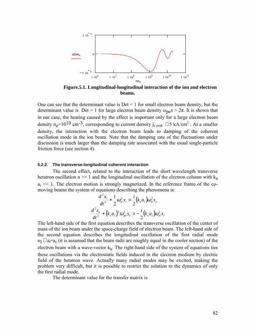
82

1 .106 1 .107 1 .108 1 .109 1 .1010 1 .10115 .10 4

0

5 .10 4

∆Detk

nek

Figure.5.1. Longitudinal-longitudinal interaction of the ion and electronbeams.

One can see that the determinant value is Det < 1 for small electron beam density, but thedeterminant value is Det > 1 for large electron beam density ωpeτ > 2π. It is shown thatin our case, the heating caused by the effect is important only for a large electron beamdensity ne=1010 cm-3, corresponding to current density je peak ≅ 5 kA/cm2 . At a smallerdensity, the interaction with the electron beam leads to damping of the coherentoscillation mode in the ion beam. Note that the damping rate of the fluctuations underdiscussion is much larger than the damping rate associated with the usual single-particlefriction force (see section 4).

5.2.2. The transverse-longitudinal coherent interactionThe second effect, related to the interaction of the short wavelength transverse

betatron oscillation n >> 1 and the longitudinal oscillation of the electron column with ksae << 1. The electron motion is strongly magnetized. In the reference frame of the co-moving beams the system of equations describing the phenomena is:

( ) eiesiiei sakix

dtxd 2

12

2

2

221 ωω =+

( ) ( ) ieisepese xakisak

dtsd 2

122

12

2

2ωω −=+

The left-hand side of the first equation describes the transverse oscillation of the center ofmass of the ion beam under the space-charge field of electron beam. The left-hand side ofthe second equation describes the longitudinal oscillation of the first radial modea1 ≅ ai=ae (it is assumed that the beam radii are roughly equal in the cooler section) of theelectron beam with a wave-vector ks. The right-hand side of the system of equations tiesthese oscillations via the electrostatic fields induced in the electron medium by electricfield of the betatron wave. Actually many radial modes may be excited, making theproblem very difficult, but it is possible to restrict the solution to the dynamics of onlythe first radial mode.

The determinant value for the transfer matrix is

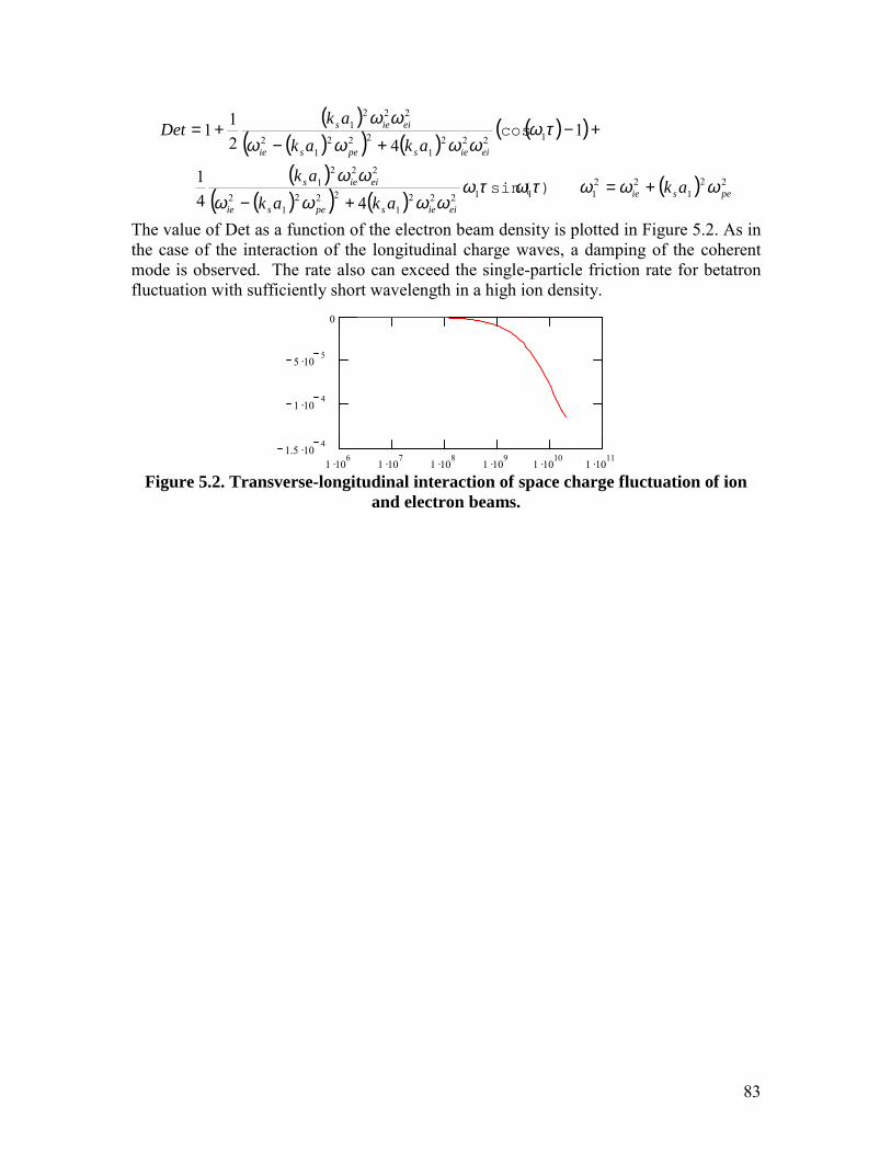
83

( )( )( ) ( )

( )( )

( )( )( ) ( )

( ) 221

22111222

1222

12

2221

12221

2221

2

2221

441

142

11

pesieeiiespesie

eiies

eiiespesie

eiies

akakak

ak

akakak

Det

ωωωτωτωωωωω

ωω

τωωωωω

ωω

+=+−

+−+−

+=

)sin(

cos

The value of Det as a function of the electron beam density is plotted in Figure 5.2. As inthe case of the interaction of the longitudinal charge waves, a damping of the coherentmode is observed. The rate also can exceed the single-particle friction rate for betatronfluctuation with sufficiently short wavelength in a high ion density.

1 .106

1 .107

1 .108

1 .109

1 .1010

1 .1011

1.5 .104

1 .104

5 .105

0

Figure 5.2. Transverse-longitudinal interaction of space charge fluctuation of ionand electron beams.

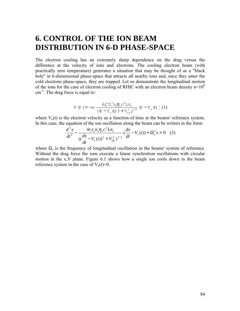
84

6. CONTROL OF THE ION BEAMDISTRIBUTION IN 6-D PHASE-SPACEThe electron cooling has an extremely sharp dependence on the drag versus thedifference at the velocity of ions and electrons. The cooling electron beam (withpractically zero temperature) generates a situation that may be thought of as a "blackhole" in 6-dimensional phase-space that attracts all nearby ions and, once they enter thecold electrons phase-space, they are trapped. Let us demonstrate the longitudinal motionof the ions for the case of electron cooling of RHIC with an electron beam density n=108

cm-3. The drag force is equal to:

))(()))(((

4)(

2/322

422

tVVVtVV

LncnZrmVF e

effe

ceeie −+−

−= η (1)

where Ve(t) is the electron velocity as a function of time at the beams' reference system.In this case, the equation of the ion oscillation along the beam can be written in the form:

0))(()))(((

4 2

2/322

2

2

2

=Ω+−+−

− xtVdtdx

VtVdtdx

Lncnrrdt

xdse

effe

ceeei η (3)

where Ωs is the frequency of longitudinal oscillation in the beams' system of reference.Without the drag force the ions execute a linear synchrotron oscillations with circularmotion in the x,V plane. Figure 6.1 shows how a single ion cools down in the beamreference system in the case of Ve(t)=0.

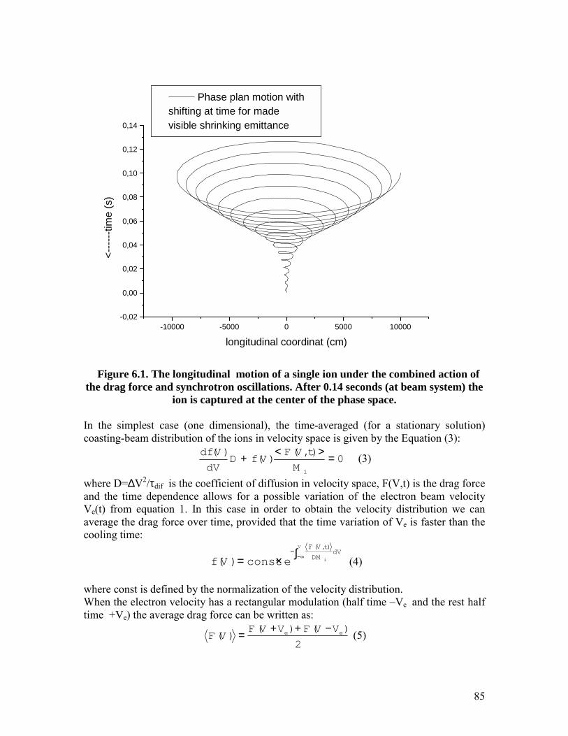
85

-10000 -5000 0 5000 10000-0,02

0,00

0,02

0,04

0,06

0,08

0,10

0,12

0,14

Phase plan motion withshifting at time for madevisible shrinking emittance

<----

--tim

e (s

)

longitudinal coordinat (cm)

Figure 6.1. The longitudinal motion of a single ion under the combined action ofthe drag force and synchrotron oscillations. After 0.14 seconds (at beam system) the

ion is captured at the center of the phase space.

In the simplest case (one dimensional), the time-averaged (for a stationary solution)coasting-beam distribution of the ions in velocity space is given by the Equation (3):

0),(

)()( =><+

iM

tVFVfD

dV

Vdf (3)

where D=∆V2/τdif is the coefficient of diffusion in velocity space, F(V,t) is the drag forceand the time dependence allows for a possible variation of the electron beam velocityVe(t) from equation 1. In this case in order to obtain the velocity distribution we canaverage the drag force over time, provided that the time variation of Ve is faster than thecooling time:

∫×= ∞−

−V

i

dVDM

tVF

econstVf

),(

)( (4)

where const is defined by the normalization of the velocity distribution.When the electron velocity has a rectangular modulation (half time –Ve and the rest halftime +Ve) the average drag force can be written as:

2

)()()( ee VVFVVF

VF−++= (5)

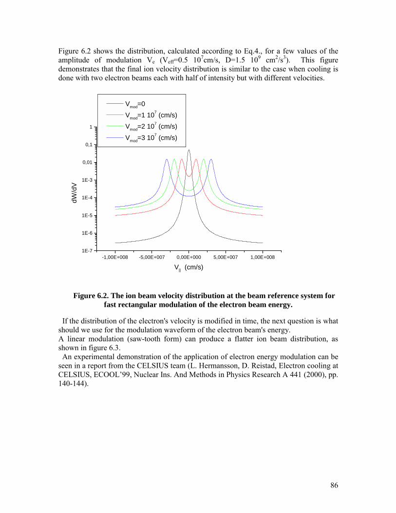
86

Figure 6.2 shows the distribution, calculated according to Eq.4., for a few values of theamplitude of modulation Ve (Veff=0.5 107cm/s, D=1.5 109 cm2/s3). This figuredemonstrates that the final ion velocity distribution is similar to the case when cooling isdone with two electron beams each with half of intensity but with different velocities.

-1,00E+008 -5,00E+007 0,00E+000 5,00E+007 1,00E+0081E-7

1E-6

1E-5

1E-4

1E-3

0,01

0,1

1

Vmod=0 Vmod=1 107 (cm/s) Vmod=2 107 (cm/s) Vmod=3 107 (cm/s)

dW/d

V

V|| (cm/s)

Figure 6.2. The ion beam velocity distribution at the beam reference system forfast rectangular modulation of the electron beam energy.

If the distribution of the electron's velocity is modified in time, the next question is whatshould we use for the modulation waveform of the electron beam's energy.A linear modulation (saw-tooth form) can produce a flatter ion beam distribution, asshown in figure 6.3. An experimental demonstration of the application of electron energy modulation can beseen in a report from the CELSIUS team (L. Hermansson, D. Reistad, Electron cooling atCELSIUS, ECOOL’99, Nuclear Ins. And Methods in Physics Research A 441 (2000), pp.140-144).

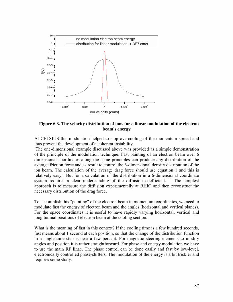
87

-1x108 -5x107 0 5x107 1x108

1E-8

1E-7

1E-6

1E-5

1E-4

1E-3

0,01

0,1

1

10 no modulation electron beam energy distribution for linear modulation +-3E7 cm/s

f(V)

ion velocity (cm/s)

Figure 6.3. The velocity distribution of ions for a linear modulation of the electronbeam's energy

At CELSIUS this modulation helped to stop overcooling of the momentum spread andthus prevent the development of a coherent instability. The one-dimensional example discussed above was provided as a simple demonstrationof the principle of the modulation technique. Fast painting of an electron beam over 6dimensional coordinates along the same principles can produce any distribution of theaverage friction force and as result to control the 6-dimensional density distribution of theion beam. The calculation of the average drag force should use equation 1 and this isrelatively easy. But for a calculation of the distribution in a 6-dimensional coordinatesystem requires a clear understanding of the diffusion coefficient. The simplestapproach is to measure the diffusion experimentally at RHIC and then reconstruct thenecessary distribution of the drag force.

To accomplish this "painting" of the electron beam in momentum coordinates, we need tomodulate fast the energy of electron beam and the angles (horizontal and vertical planes).For the space coordinates it is useful to have rapidly varying horizontal, vertical andlongitudinal positions of electron beam at the cooling section.

What is the meaning of fast in this context? If the cooling time is a few hundred seconds,fast means about 1 second at each position, so that the change of the distribution functionin a single time step is near a few percent. For magnetic steering elements to modifyangles and position it is rather straightforward. For phase and energy modulation we haveto use the main RF linac. The phase control can be done easily and fast by low-level,electronically controlled phase-shifters. The modulation of the energy is a bit trickier andrequires some study.

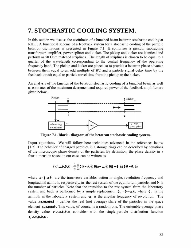
88

7. STOCHASTIC COOLING SYSTEM.In this section we discuss the usefulness of a bunched beam betatron stochastic cooling atRHIC. A functional scheme of a feedback system for a stochastic cooling of the particlebetatron oscillations is presented in Figure 7.1. It comprises a pickup, subtractingtransformer, amplifier, power splitter and kicker. The pickup and kicker are identical andperform as 50 Ohm matched striplines. The length of striplines is chosen to be equal to aquarter of the wavelength corresponding to the central frequency of the operatingfrequency band. The pickup and kicker are placed so to provide a betatron phase advancebetween them equal to an odd multiple of π/2 and a particle signal delay time by thefeedback circuit equal to particle travel time from the pickup to the kicker.

An analysis of the kinetics of the betatron stochastic cooling of a bunched beam as wellas estimates of the maximum decrement and required power of the feedback amplifier aregiven below.

Δx

Pickup

subtracting transformer

2 – way power splitter

Kicker

Amp

Figure 7.1. Block - diagram of the betatron stochastic cooling system.

Input equations. We will follow here techniques advanced in the references below[1,2]. The behavior of charged particles in a storage rings can be described by equationsof the microscopic phase density of the particles. By definition, the phase density in afour-dimension space, in our case, can be written as

∑∑∑∑ ϑϑϑϑ−−−−ϑϑϑϑδδδδϕϕϕϕ−−−−ϕϕϕϕδδδδωωωω−−−−ωωωωδδδδ−−−−δδδδ====ϑϑϑϑϕϕϕϕωωωω====

N

1iiiii )]t([)]t([)]t([)]t(JJ[

N

1)t,,,,J(F

where ϑϑϑϑωωωωϕϕϕϕ ,,−J are the transverse variables action in angle, revolution frequency andlongitudinal azimuth, respectively, in the rest system of the equilibrium particle, and N isthe number of particles. Note that the transition to the rest system from the laboratorysystem and back is performed by a simple replacement tL 0ωωωωϑϑϑϑϑϑϑϑ += , where Lϑϑϑϑ is theazimuth in the laboratory system and 0ωωωω is the angular frequency of revolution. Thevalue ϑϑϑϑϕϕϕϕωωωω ddFdJd - defines the real (not average) share of the particles in the spaceelement ϑϑϑϑϕϕϕϕωωωω dddJd . This value, of course, is a random one. The ensemble-average phasedensity value )t,,,,J(F ϑϑϑϑϕϕϕϕωωωω coincides with the single-particle distribution function

)t,,,,J(f1 ϑϑϑϑϕϕϕϕωωωω .

89

The phase density evolution is determined by the equation

0JFJFFF

tF =

∂∂+

ω∂∂ω+

ϑ∂∂ϑ+

ϕ∂∂ϕ+

∂∂ #### (1)

Let us designate the phase density deviations from their average values as

)t,,,,J(F)t,,,,J(F)t,,,,J(f 1 ϑϑϑϑϕϕϕϕωωωω−−−−ϑϑϑϑϕϕϕϕωωωω====ϑϑϑϑϕϕϕϕωωωωδδδδ .

After averaging the ensemble, equation (1) gives the equations for the distributionfunction 1F and Fδδδδ

(2)

J

fJ

J

fJ

J

fJ

fff

t

f 1

∂∂∂∂δδδδ∂∂∂∂++++

∂∂∂∂δδδδ∂∂∂∂−−−−====

∂∂∂∂∂∂∂∂

++++ωωωω∂∂∂∂δδδδ∂∂∂∂ωωωω++++

ϑϑϑϑ∂∂∂∂δδδδ∂∂∂∂ϑϑϑϑ++++

ϕϕϕϕ∂∂∂∂δδδδ∂∂∂∂ϕϕϕϕ++++

∂∂∂∂δδδδ∂∂∂∂ ###### (3)

Model of the interaction. The particle motion equations, written down in the rest systemof the equilibrium particle, are of the form:

ΩΩΩΩ====ϕϕϕϕ#

ϕϕϕϕΜΩΜΩΜΩΜΩ

ϕϕϕϕΜΩΜΩΜΩΜΩ

cos2

2cos)(2

xyx EJ

qvBEJ

qJ =−=# (4)

ωωωω====ϑϑϑϑ#

where ΩΩΩΩΜΜΜΜ ,,q are the mass, charge and angular betatron frequency of the particle,respectively. We assume here that the main mechanism of the particles-mixing is therevolution frequency spread of particles.

The transverse electric field created by a kicker, )t,t(E 0x ωωωω++++ϑϑϑϑ , is expressed by the Fourierexpansion:

)tm(im

mm

00x

0eaa2

)t(UR2L)t,t(E ω+ϑ∑π

=ω+ϑ (5)

where )t(U,a,R,L 0 are the kicker length, ring average radius, kicker half-aperture andvoltage between kicker striplines, respectively. The coefficients ma take into account thefield distribution in the kicker. For simplicity, let ma be equal to unity.

Let us assume that the particle interaction via feedback is small and that the decisive rolein the interaction is provided by beam azimuth harmonics with length much less than theazimuth bunch length. Under this assumption, upon the integration of equation (3), it ispossible to take ignore the ϑϑϑϑ,t dependence of the single-participle distribution function.

90

We suppose also that the correlation time of the feedback signal is much less than theperiod of particle synchrotron oscillations and 0====ωωωω# . Neglecting non-linear terms, we canwrite down (3) as follows

J

fJ

ff

t

f 1

∂∂∂∂∂∂∂∂

−−−−====ϑϑϑϑ∂∂∂∂δδδδ∂∂∂∂ϑϑϑϑ++++

ϕϕϕϕ∂∂∂∂δδδδ∂∂∂∂ϕϕϕϕ++++

∂∂∂∂δδδδ∂∂∂∂ ### . (6)

Equation (6) is a usual linear equation with respect to fluctuations. Its complete solutionis, as known, the sum of the free solution, determined by the initial condition, and of theforced one. However, it is more convenient to consider the initial conditions being zeroand to introduce into (6) a source, equivalent to them. Taking into account (4), (5) wehave

∑∂∂

−=−∂∂+

∂∂+

∂∂ +

m

timsrc eJ

fJ

a

tU

R

qLff

t)(1

0

0cos2)(

2))(( ωωωωϑϑϑϑϕϕϕϕ

ΜΩΜΩΜΩΜΩππππδδδδδδδδ

ϑϑϑϑϑϑϑϑ

ϕϕϕϕϕϕϕϕ ## (7)

The source fluctuations srcfδδδδ are the free fluctuations fδδδδ when there is no interaction. Thesource correlation function is determined by the relation [1]

====ττττ−−−−ϑϑϑϑ ′′′′ϕϕϕϕ ′′′′ωωωω′′′′′′′′δδδδϑϑϑϑϕϕϕϕωωωωδδδδ )t,,,,J(f)t,,,,J(f srcsrc

),,,J(f)()()()JJ(N

11 ϑϑϑϑϕϕϕϕωωωωωτωτωτωτ−−−−ϑϑϑϑ ′′′′−−−−ϑϑϑϑδδδδττττΩΩΩΩ−−−−ϕϕϕϕ ′′′′−−−−ϕϕϕϕδδδδωωωω′′′′−−−−ωωωωδδδδ′′′′−−−−δδδδ==== . (8)

The solution of the equation (7) can be presented after Laplace transformation infollowing form

srcmm f

iimsJ

f

a

imsUJ

R

qLsJf 1,

10

01,

1

2

)(2

2),,( ±± +

±+∂∂−

−= δδδδΩΩΩΩωωωω

ωωωωΜΩΜΩΜΩΜΩππππ

ωωωωδδδδ , (9)

where ∫∫∫∫ ϑϑϑϑϕϕϕϕωωωωϑδϑδϑδϑδϕϕϕϕππππ

====δδδδ ϕϕϕϕϑϑϑϑ−−−−±±±±

iim

21,m e)s,,,,J(fdd)2(

1f $ , and sis a variable in a Laplace image.

Taking into account the relative position of the pickup and kicker and the betatronphase advance between them, the feedback voltage on the kicker is of the form

∑∑∑∑ ωωωω++++====m

0m )ims(x)s(K)s(U , (10)

where ∫ +=∫= − ωωωωδδδδδδδδΜΩΜΩΜΩΜΩ

ππππϕϕϕϕωωωωδδδδϕϕϕϕΜΩΜΩΜΩΜΩ

dJdffJ

ddJdfJ

sx mmmm )(2

cos2

)( 1,1,

and )s(K - a gain from the pickup to the kicker. From (9),(10) one can obtain that

)s()ims(K1

xx

m0

srcm

m ηηηηωωωω−−−−−−−−==== , (11)

91

∫ =−+

+++∂

∂−= ωωωω

ΩΩΩΩωωωωΩΩΩΩωωωωΜΩΜΩΜΩΜΩηηηη dJd

iimsiimsJ

fJ

aR

qLsm )

11(

21

0)(

∫ −++

++−= ωωωω

ΩΩΩΩωωωωΩΩΩΩωωωωΜΩΜΩΜΩΜΩd

iimsiimsf

aR

qL)

11(

2 10

. (12)

Cooling decrement. Return to equation (2). Assuming that there is no influence of theparticle transverse motion on the longitudinal one in the left-hand side of (2) only a timederivative should be left. Writing down the right-hand side of (2) in detailed form wehave

ϑϑϑϑωωωωϑϑϑϑ δδδδϕϕϕϕΜΩΜΩΜΩΜΩππππ

mim

mm

tim efJ

eJ

a

tU

R

qL

t

f ′−′−

′

+

∂∂

∑−=∂∂

,

)(

0

1 0cos2)(

2

Averaging the right-hand side of the last equation over ϑϑϑϑϕϕϕϕ, one can obtain

)(2

2

)(

2 1,1,0

1 0−−− +

∂∂

∑−=∂∂

mmm

tim ffJ

eJ

a

tU

R

qL

t

fδδδδδδδδ

ΜΩΜΩΜΩΜΩππππωωωω (13)

Substitute (9) in (13), then multiply (13) by Jand carry out integration over ωωωω,J . Theresult can be written down in the following form

)()]()([2

1

22

3),(

,0

1

01 txsxmisKL

aR

qLtJ

tdJdJf

tm

mmm −

′′

−∑ ′−−=∫ ⟩⟨∂∂=

∂∂ ωωωω

ππππππππϑϑϑϑωωωω , (14)

[.L 1−−−− - a Laplace inverse transform.

Under the assumption made above, the interaction process can be considered as astationary one and ensemble averaging in (14) can be replaced by time averaging. Let

maxm be maximum number of operating azimuth of harmonics and 0max 5.0 ωωωωωωωω∆∆∆∆ ≤m (a weakmixing), ωωωω∆∆∆∆ - the particles revolution frequency spread. In this case there is no correlationbetween the center of gravity harmonics with different numbers and in (14) one shouldleft the terms with mm ′′′′==== . Following [1] it can be shown that

∫∫∫∫ ωωωω−−−−φφφφφφφφφφφφ====ωωωω−−−−∞∞∞∞

∞∞∞∞−−−−−−−−

−−−− )imi(K)(Sd)t(x)]s(x)ims(K[L 0m,xmm01 ,

where m,xS is a spectral density of the center of gravity fluctuations. For the stationary

process

2

)00m

srcm,x

m,x

imi(K)imi(1

)(S)(S

ωωωω−−−−φφφφ−−−−ωωωω−−−−φφφφ−−−−ηηηη−−−−

φφφφ====φφφφ ,

92

srcm,xS is the spectral density of free fluctuations of the center of gravity. Taking into

account (8), (10) one can obtain that

∫ +++−+= ωωωωΩΩΩΩωωωωφφφφδδδδΩΩΩΩωωωωφφφφδδδδϑϑϑϑωωωωΜΩΜΩΜΩΜΩ

φφφφ dJdmmJJfN

Ssrcmx )]()()[,,(

2

1)( 1, .

Summing these results, we write down the final equation described the betatronstochastic cooling of a bunched beam

∫ ∑−++−

−+=⟩⟨

∂∂

mm imimiKimi

imimiKdJdtJJf

aNR

qLtJ

t 2

0

01

0 ()(1

)(Re[),,,(

2),(

ωωωωωωωωΩΩΩΩωωωωΩΩΩΩηηηη

ωωωωωωωωΩΩΩΩωωωωϑϑϑϑωωωω

ΜΩΜΩΜΩΜΩππππππππϑϑϑϑ (15)

So as one can see the cooling decrement is equal to the sum of partial decrements of thebetatron sidebands around the harmonics of the revolution frequency.

Estimates. Assuming that the length of striplines is chosen to be equal to quarter of thewavelength corresponding to a central frequency of a operating frequency band andoperating frequency band is of the order of a few GHz

a

imKqNimKimimiK fb )(

)()( 0000

ωωωωρρρρωωωωωωωωωωωωΩΩΩΩΩΩΩΩ

−=−≈−+ ,

)( 0ωωωωimK fb is the voltage gain of the feedback, including the pickup and kickertransmission coefficient and feedback amplifiers gain, ρρρρ is the kicker and pickupstriplines wave impedance. Taking into account only resonance term in the expression for

)imi(m ωωωω++++ΩΩΩΩηηηη we have

∫ ′+′′

−=+ ]),(),(

[2

)( 11

0 ωωωωωωωωωωωωϑϑϑϑωωωωϑϑϑϑωωωωππππ

ΜΩΜΩΜΩΜΩωωωωΩΩΩΩηηηη

mm

dfi

m

f

Ra

qLimim (16)

For an estimate, let us leave in (16) only the first term

ϑϑϑϑ∆∆∆∆ωωωω∆∆∆∆ππππΜΩΜΩΜΩΜΩππππϑϑϑϑωωωω

ΜΩΜΩΜΩΜΩππππωωωωΩΩΩΩηηηη

2

1

2

),(

2)(

0

1

0 mRa

qL

m

f

Ra

qLimi ≈≈+ , (17)

where ϑϑϑϑ∆∆∆∆ωωωω∆∆∆∆ , are the bunch revolution frequency spread and azimuth length,accordingly.

The frequency bandwidth of the feedback is determined by the bandwidth of the pickupand kicker and in our case is, approximately, one octave (mmax/mmin=2). Then let L beR0/mmax. As a result, equation (15) takes the form

∑+

≈∂

∂ max

max

22)

21(

2),(

),( m

m

m

m

m

NtJ

t

tJ

ωωωω∆∆∆∆ϑϑϑϑ∆∆∆∆ππππλλλλ

λλλλϑϑϑϑ

ϑϑϑϑ , max

2

2

2

1

m

K

a

Nq fbm ΩΩΩΩΜΜΜΜ

ρρρρππππ

λλλλ = .

93

It is clear that a maximum decrement ,maxδδδδ is obtained when 12 =

mm ωωωω∆∆∆∆ϑϑϑϑ∆∆∆∆

ππππλλλλ . In this case

N

fm

ππππϑϑϑϑ∆∆∆∆∆∆∆∆δδδδ

2

2max

max = (18)

This expression determines the possibility of using a feedback system for cooling theparticles’ transverse oscillations. It can be shown that the same expression defines thepossibility of the stochastic cooling of the particles’ longitudinal motion as well. This isunderstandable because in both cases the mixing mechanism is the particles revolutionfrequency spread.

In conclusion, let us make an estimate of a noise power of the beam particle center ofgravity fluctuations on the pickup output when the feedback is off.

∑= −m

srcm

srcmbeamin txtx

a

NqP )()()(

1 20,

ρωρωρωρωρρρρ

.

After averaging for the one octave feedback frequency bandwidth we have

2

2)( max

2

2

20,

m

a

xqf

NP beamin ϑϑϑϑ∆∆∆∆

ππππ∆∆∆∆ρρρρ

ρρρρ= ,

where 2x∆∆∆∆ - rms of the betatron beam size.]

The noise power of the electronics on the pickup output is determined by the well knownexpression

24 max

0,

mFkTfP nelin = ,

where nF is the electronics noise figure.

The following are the values relevant for RHIC:

Revolution frequency, kHz 78Tunes, νx/ νy 28.18/29.18Ion (gold) beam energy spread 4*10-4

Ion beam revolution frequency spread 5*10-7

Number of the ion per bunch 109

Ion energy per nucleon, GeV 100Ion beam length, m 0.3Average betatron beam size, m 4.5*10-4

Feedback frequency band, GHz 3÷6Maximum decrement,sec-1 1/105

94

Pin,beam , W 3*10-9

Pin,el, W 2*10-10

Feedback gain 3*104

Conclusion. As one can see the maximum decrement of the cooling of the transverseparticles motion as well as longitudinal one is of the order of 30 hours. The beam lifetimein colliding mode at RHIC is about 10 hours. It is obvious that in this case stochasticcooling is not effective.

References1. N.I. Zinevich, M.M. Karliner. Kinetic equation of the stochastic cooling of thelongitudinal momentum spread. 8 international proceeding on high energy accelerators,Protvino, 1982.2. 2.Yu.l.Klimontovich. Kinetic theory of a non-ideal gas and non-ideal plasma.Moscow, 1975.

95

8. CONSIDERATIONS TOWARDS A CDR The electron cooling of RHIC will take a very large step in energy compared withconventional electron cooling. The highest electron energy cooler now is CELSIUS, atabout 300 kV. An experiment with a high energy, high current electron beam, but withoutcooling, was made at BINP many years ago, reaching an energy of 1MeV with anelectron current of 1A. The Fermilab electron cooling project for antiprotons, at anelectron energy of 5 MeV, is now under development and results should be clear in 3-4years. RF-type accelerators for FEL experiments with very high brightness electronbeam and with energy in the range of 10-50 MeV are now under development in manylaboratories. However, for electron cooling we need a magnetized beam and for thegeneration of this beam in a magnetic field precludes using a superconducting electrongun. At the same time, a high voltage CW copper cavity gun is very large andexpensive.

Key items and some comments for the CDR study.

For this project the parameters of the electron gun should be:a. Repetition frequency 4.6 MHz,b. Number of electrons per bunch Ne=1011 , charge 16 nC,c. Pulse length 1-4 ns,d. Peak current Je=4-16 A,e. The cathode of the electron gun should be immersed in a magnetic field of about

100 G.

The electron emission control may be a grid control or a semiconductor photocathodecathode under laser beam control. The laser system for this electron gun needs R&Dbecause of the very high charge of 16 nC. The final decision should be made between theversion of injection system based on DC acceleration system or low frequency RF cavity.For low beam intensity of 1010 –3x1010 electrons per bunch, an energy of 2 MeV isenough but for a high intensity beam, 1011, it is required to upgrade the injection energyto 4-5 MeV.

1. Development of the electron gun and initial accelerator.a. Development of the electron DC accelerator.b. Development of the low frequency CW cavity for acceleration.c. Development of the photocathode of the gun.d. Development of the laser system.

2. Development of the accelerator and beam transport elements:a. Development of the debuncher - rebuncher beam transport elements and cavities

with a detailed 6-D simulation of the electron beam dynamics.b. Demonstration of the energy recovery linac at the current of the cooler and with

appropriate beam performance.

96

c. Investigation of feedback techniques for stabilizing the linac.d. Detail development of magnetized electron generation and transport. The

development of alternative approaches for the transport of a flat or a round(magnetized) beam.

3. Development of the solenoida. Development of the high-precision superconducting solenoidb. Development of magnetic field measuring techniques for a superconducting, high

precision solenoidc. Development of the beam matching sections at either end of the solenoid.d. Development of electron / ion beam diagnostics for the solenoid section.

4. Cooling theoretical studies: a. Control of the longitudinal / transverse cooling decrement b. Shaping the 6-D beam by control of the electron beam c. Optimization of the cooler parameters d. Beam-Beam effect under electron cooling e. Coherent effects in the system of ion bunches –the cooling electron beam

f. An experiment with cooling in high magnetic fields and high transverse electronbeam temperature in a low energy cooler (if possible to find time for theseexperiments on existing ring CELSIUS, GSI, Indiana).

g. Theoretical and experimental investigation of IBS.

Electron beam generator in experiment at BINPA high-power infrared free electron laser is under construction in Novosibirsk.

The list of parameter of this device is shown in table1.

Table 1. Main parameters of FEL device at BINP (Novosibirsk)

Machine itself:RF accelerating frequency, MHz 180Number of RF-cavities 16Amplitude of accelerating voltage per cavity, MV up to 0.8Total RF-power, MW up to 1.2Injection and extraction energy (full), MeV 2

Accelerated beam:Bunch repetition rate, MHz up to 22.5Average electron current, mA up to 50Electron energy, MeV up to 100Electron energy spread (relative) 10-3

Bunch duration, ps 10...20Peak current, A 100...200

97

RF-Cavities Bending Magnets Quadrupoles Solenoids

Undulators Bunchers Gun Dump

Figure 8.1. The sketch of FEL device at BINP NovosibirskThe first stage of this project with one turn of electron beam should be commissioned in2001. Within the frame of this project, it is possible to have collaboration for thedevelopment of common elements of BNL cooler system and FEL at BINP:

1. A 2-MeV thermionic electron gun with a solenoid and a beam shape converter.2. A RF-buncher with bunching RF-cavities, RF-generators, and bending magnets.3. RF-cavities and RF-generators for compensating the correlated energy spread gained

in the main accelerating structure and necessary for debunching.4. RF-cavities and RF-generators for compensating the cubic term of correlated energy

spread gained in the buncher.5. Magnetic elements (lenses, bending magnets, solenoid) for the whole machine.6. RF-generators for the main accelerating structure.R&D according to the mentioned items1. Gun

• A prototype of the cathode-grid unit with a manipulator.• Beam measurements in the ready machine used as a prototype.• A prototype of a 2-MeV power supply and accelerating tube.• Numerical simulation of electron motion in the gun and the beam shape

converter (3D, transient, space charge effect).• A prototype of the beam measurement system (emittance, dispersion function,

energy spread, time structure)2. Buncher

• Numerical simulation of the bending magnet with gradient and sextupolecorrection (3D).

• Numerical simulation of electron motion in the buncher (3D, transient, spacecharge effect).

• Prototypes of RF-cavities and RF-generators of the buncher.3. Prototypes of the compensating RF-cavities and the RF-generators.4. Prototypes of the compensating RF-cavities and the RF-generators.

98

5. Numerical simulation of the magnetic elements and electron motion through the wholemachine.

6. A prototype of the RF-generators.

V. Parkhomchuk I. Ben-Zvi - Brookhaven National Laboratory · · 2013-01-292/ρ2 ×2 ρ/V. The...

Documents

Transcript of V. Parkhomchuk I. Ben-Zvi - Brookhaven National Laboratory · · 2013-01-292/ρ2 ×2 ρ/V. The...