UniversitédeMontréal - core.ac.uk · φm et φk.Lescoefﬁcients ck,où kvariede 1...

Université de Montréal

Étude de dispositifs électroniques moléculaires à l’aide de modèles simples

parPhilippe Rocheleau

Département de chimieFaculté des arts et des sciences

Thèse présentée à la Faculté des études supérieures et postdoctoralesen vue de l’obtention du grade de Philosophiæ Doctor (Ph.D.)

en chimie

Mai, 2014

c© Philippe Rocheleau, 2014.

RÉSUMÉ

Cette thèse en électronique moléculaire porte essentiellement sur le développement

d’une méthode pour le calcul de la transmission de dispositifs électroniques molécu-

laires (DEMs), c’est-à-dire des molécules branchées à des contacts qui forment un dis-

positif électronique de taille moléculaire. D’une part, la méthode développée vise à

apporter un point de vue différent de celui provenant des méthodes déjà existantes pour

ce type de calculs. D’autre part, elle permet d’intégrer de manière rigoureuse des outils

théoriques déjà développés dans le but d’augmenter la qualité des calculs. Les exemples

simples présentés dans ce travail permettent de mettre en lumière certains phénomènes,

tel que l’interférence destructive dans les dispositifs électroniques moléculaires.

Les chapitres proviennent d’articles publiés dans la littérature. Au chapitre 2, nous étu-

dions à l’aide d’un modèle fini avec la méthode de la théorie de la fonctionnelle de

la densité de Kohn-Sham un point quantique moléculaire. De plus, nous calculons la

conductance du point quantique moléculaire avec une implémentation de la formule

de Landauer. Nous trouvons que la structure électronique et la conductance molécu-

laire dépendent fortement de la fonctionnelle d’échange et de corrélation employée.

Au chapitre 3, nous discutons de l’effet de l’ajout d’une chaîne ramifiée à des molé-

cules conductrices sur la probabilité de transmission de dispositifs électroniques mo-

léculaires. Nous trouvons que des interférences destructives apparaissent aux valeurs

propres de l’énergie des chaînes ramifiées isolées, si ces valeurs ne correspondent pas

à des états localisés éloignés du conducteur moléculaire. Au chapitre 4, nous montrons

que les dispositifs électroniques moléculaires contenant une molécule aromatique pré-

sentent généralement des courants circulaires qui sont associés aux phénomènes d’in-

terférence destructive dans ces systèmes. Au chapitre 5, nous employons l’approche

« source-sink potential » (SSP) pour étudier la transmission de dispositifs électroniques

moléculaires. Au lieu de considérer les potentiels de sources et de drains exactement,

nous utilisons la théorie des perturbations pour trouver une expression de la probabi-

iii

lité de transmission, T (E) = 1 − |r(E)|2, où r(E) est le coefficient de réflexion quidépend de l’énergie. Cette expression dépend des propriétés de la molécule isolée, en

effet nous montrons que c’est la densité orbitalaire sur les atomes de la molécule qui

sont connectés aux contacts qui détermine principalement la transmission du dispositif

à une énergie de l’électron incident donnée. Au chapitre 6, nous présentons une exten-

sion de l’approche SSP à un canal pour des dispositifs électroniques moléculaires à

plusieurs canaux. La méthode à multiples canaux proposée repose sur une description

des canaux propres des états conducteurs du dispositif électronique moléculaire (DEM)

qui sont obtenus par un algorithme auto-cohérent. Finalement, nous utilisons le modèle

développé afin d’étudier la transmission du 1-phényl-1,3-butadiène branché à deux ran-

gées d’atomes couplées agissant comme contacts à gauche et à la droite.

Mots-Clés : Électronique moléculaire, effet de Kondo, transmission électronique,

conductance moléculaire, interférence, source-sink potential.

ABSTRACT

This thesis is on molecular electronics concentrates mostly on the development of

a method for the calculation of the transmission probability of molecules that are con-

nected to contacts. On the one hand, this method aims at bringing a different point of

view among the other methods for such calculations. On the other hand, it allows the

integration of already developed theoretical tools in a rigorous manner, which increases

the quality of the calculations. The work presented here often contains simple examples

that shine some light on phenomena, such as the destructive interference, in molecular

electronic devices.

The chapters are from articles already published in the litterature. In chapter 2, we study

a molecular quantum dot using a finite model with Kohn-Sham density functional the-

ory. Moreover, using an implementation of the Landauer formula, we calculate the

conductance of the quantum dot. We find that the electronic structure and molecular

conductance depend strongly on the exchange and correlation functional employed. In

chapter 3, we discuss the effect of adding a side chain to conducting molecules on the

transmission probability of molecular electronic devices. We find that destructive in-

terferences appear approximately at the energy eigenvalues of the isolated side chain,

if these values do not correspond to localized states far away from the conductor. In

chapter 4, we show that molecular electronic devices containing an aromatic molecule

generaly possess circular currents which are associated with destructive interference

phenomena in these systems. In chapter 5, we use the source-sink potential (SSP) ap-

proach to study the electronic transmission of some devices. Instead of considering

the source and sink potentials exactly, we use perturbation theory to find an expression

for the transmission probability T (E) = 1− |r(E)|2 that depends on the properties ofthe bare molecule, where r(E) is the energy-dependent reflection coefficient. We show

that in the first-order, it is the orbital density on the atoms connected to the contacts

that largely determines the transmission probability for a given incoming electron en-

v

ergy. In chapter 6, we present an extension of the single channel source-sink potential

approach for molecular electronic devices to multiple channels. The proposed multi-

channel method relies on an eigenchannel description of the conducting states of the

molecular electronic device, which are obtained by a self-consistent algorithm. We use

the model to study the transport of the 1-phenyl-1,3-butadiene molecule connected to

two coupled rows of atoms that act as contacts on the left and right sides.

Keywords: Molecular electronics, Kondo effect, electronic transmission, molecu-

lar conductance, interference, source-sink potential.

vi

TABLE DES MATIÈRES

RÉSUMÉ . . . . . . . . . . . . . . . . . . . . . . . . . . . . . . . . . . . . ii

ABSTRACT . . . . . . . . . . . . . . . . . . . . . . . . . . . . . . . . . . . iv

TABLE DES MATIÈRES . . . . . . . . . . . . . . . . . . . . . . . . . . . vi

LISTE DES TABLEAUX . . . . . . . . . . . . . . . . . . . . . . . . . . . x

LISTE DES FIGURES . . . . . . . . . . . . . . . . . . . . . . . . . . . . xi

LISTE DES SIGLES . . . . . . . . . . . . . . . . . . . . . . . . . . . . . . xiv

REMERCIEMENTS . . . . . . . . . . . . . . . . . . . . . . . . . . . . . xv

INTRODUCTION . . . . . . . . . . . . . . . . . . . . . . . . . . . . . . . 1

1.1 Objectifs de la thèse . . . . . . . . . . . . . . . . . . . . . . . . . . . . 1

1.2 Mise en contexte . . . . . . . . . . . . . . . . . . . . . . . . . . . . . 1

1.3 Transport en électronique moléculaire . . . . . . . . . . . . . . . . . . 5

1.3.1 Rappel du modèle Hückel . . . . . . . . . . . . . . . . . . . . 7

1.3.2 Méthode source-sink potential (SSP) pour le calcul de la conduc-

tance . . . . . . . . . . . . . . . . . . . . . . . . . . . . . . . 10

1.3.3 Autres méthodes de calculs de la conductance . . . . . . . . . . 18

1.4 Pertinence des travaux . . . . . . . . . . . . . . . . . . . . . . . . . . 21

1.5 Contenu des chapitres . . . . . . . . . . . . . . . . . . . . . . . . . . . 22

1.6 Bibliographie . . . . . . . . . . . . . . . . . . . . . . . . . . . . . . . 24

CHAPITRE 2: APPROXIMATEDENSITY FUNCTIONALSAPPLIED TO

MOLECULAR QUANTUM DOTS . . . . . . . . . . . . 31

Contribution des coauteurs . . . . . . . . . . . . . . . . . . . . . . . . . . . 32

Abstract . . . . . . . . . . . . . . . . . . . . . . . . . . . . . . . . . . . . . 33

2.1 Introduction . . . . . . . . . . . . . . . . . . . . . . . . . . . . . . . . 34

vii

2.2 Theory . . . . . . . . . . . . . . . . . . . . . . . . . . . . . . . . . . . 36

2.3 Computational results and their interpretation . . . . . . . . . . . . . . 39

2.4 Conclusion . . . . . . . . . . . . . . . . . . . . . . . . . . . . . . . . 44

2.5 Bibliography . . . . . . . . . . . . . . . . . . . . . . . . . . . . . . . 46

CHAPITRE 3: SIDE-CHAIN EFFECTS IN MOLECULAR DEVICES . 48


Abstract . . . . . . . . . . . . . . . . . . . . . . . . . . . . . . . . . . . . . 50

3.1 Introduction . . . . . . . . . . . . . . . . . . . . . . . . . . . . . . . . 51

3.2 Summary of theoretical tools . . . . . . . . . . . . . . . . . . . . . . . 52

3.3 Transmission through molecules with side chains . . . . . . . . . . . . 54

3.4 Kohn-Sham calculations for a molecular conductor with large side chain 59

3.5 Discussion and conclusion . . . . . . . . . . . . . . . . . . . . . . . . 60

3.6 Bibliography . . . . . . . . . . . . . . . . . . . . . . . . . . . . . . . 63

CHAPITRE 4: ELECTRONTRANSMISSION THROUGHAROMATICMO-

LECULES . . . . . . . . . . . . . . . . . . . . . . . . . 65


Abstract . . . . . . . . . . . . . . . . . . . . . . . . . . . . . . . . . . . . . 67

4.1 Introduction . . . . . . . . . . . . . . . . . . . . . . . . . . . . . . . . 68

4.2 Summary of theoretical concepts . . . . . . . . . . . . . . . . . . . . . 69

4.3 Benzene molecule . . . . . . . . . . . . . . . . . . . . . . . . . . . . . 73

4.4 Coronene molecule . . . . . . . . . . . . . . . . . . . . . . . . . . . . 76

4.5 Observable consequences of the predicted circular currents . . . . . . . 79

4.6 Discussion and conclusion . . . . . . . . . . . . . . . . . . . . . . . . 81

4.7 Bibliography . . . . . . . . . . . . . . . . . . . . . . . . . . . . . . . 84

CHAPITRE 5: MOLECULAR CONDUCTANCE OBTAINED IN TERMS

OFORBITALDENSITIES ANDRESPONSE FUNCTIONS 86


Abstract . . . . . . . . . . . . . . . . . . . . . . . . . . . . . . . . . . . . . 88

viii

5.1 Introduction . . . . . . . . . . . . . . . . . . . . . . . . . . . . . . . . 89

5.2 Perturbative approach to the transmission probability . . . . . . . . . . 91

5.3 Explicit expressions within the Hückel model . . . . . . . . . . . . . . 93

5.4 Wide band limit of the first-order approximation . . . . . . . . . . . . . 96

5.5 Second-order perturbation expression . . . . . . . . . . . . . . . . . . 97

5.6 Applications of the perturbative approach . . . . . . . . . . . . . . . . 100

5.7 Extension to an interacting system . . . . . . . . . . . . . . . . . . . . 103

5.8 Conclusions . . . . . . . . . . . . . . . . . . . . . . . . . . . . . . . . 105

5.9 Bibliography . . . . . . . . . . . . . . . . . . . . . . . . . . . . . . . 106

CHAPITRE 6: EXTENSION OF THE SOURCE-SINK POTENTIAL (SSP)

APPROACH TO MULTICHANNEL QUANTUM TRANS-

PORT . . . . . . . . . . . . . . . . . . . . . . . . . . . . 109


Abstract . . . . . . . . . . . . . . . . . . . . . . . . . . . . . . . . . . . . . 111

6.1 Introduction . . . . . . . . . . . . . . . . . . . . . . . . . . . . . . . . 112

6.2 Derivation of the multichannel source-sink potential approach . . . . . 114

6.3 Complex potentials for two coupled monoatomic chains in the Hückel

approximation . . . . . . . . . . . . . . . . . . . . . . . . . . . . . . . 115

6.4 Eigenchannel search algorithm . . . . . . . . . . . . . . . . . . . . . . 119

6.5 Multichannel transmission through phenylbutadiene . . . . . . . . . . . 122

6.6 Conclusion . . . . . . . . . . . . . . . . . . . . . . . . . . . . . . . . 129

6.7 Bibliography . . . . . . . . . . . . . . . . . . . . . . . . . . . . . . . 130

CONCLUSION . . . . . . . . . . . . . . . . . . . . . . . . . . . . . . . . . 133

7.1 Synthèse et discussion générale des résultats . . . . . . . . . . . . . . . 133

7.1.1 Aperçu des limites d’applicabilité de la méthode NEGF pour la

transmission de DEMs . . . . . . . . . . . . . . . . . . . . . . 134

7.1.2 Phénomène d’interférence destructive dans la transmission de

molécules conjuguées linéaires et aromatiques . . . . . . . . . 136

7.1.3 Améliorations apportées à la méthode SSP . . . . . . . . . . . 141

ix

7.1.4 Apport de la théorie des graphes . . . . . . . . . . . . . . . . . 143

7.2 Perspectives générales . . . . . . . . . . . . . . . . . . . . . . . . . . 144

7.2.1 Intérêt de la méthode SSP . . . . . . . . . . . . . . . . . . . . 144

7.2.2 Limites de la méthode Hückel . . . . . . . . . . . . . . . . . . 145

7.2.3 Perspectives associées à la DFT dans nos travaux . . . . . . . . 146

7.2.4 Perspectives associées aux effets d’interférence et aux règles

simples établies pour la transmission de DEMs . . . . . . . . . 146

7.2.5 Perspectives associées à l’extension de la méthode SSP à plu-

sieurs canaux . . . . . . . . . . . . . . . . . . . . . . . . . . . 147

7.2.6 Nature statistique des expériences et spectroscopie de DEM in-

dividuel . . . . . . . . . . . . . . . . . . . . . . . . . . . . . . 148

7.2.7 Autres types de DEMs et aspects à considérer dans leur étude . 148

7.2.8 Considérations pratiques et utilité réelle des DEMs . . . . . . . 149

7.2.9 Mot de la fin . . . . . . . . . . . . . . . . . . . . . . . . . . . 150

7.3 Bibliographie . . . . . . . . . . . . . . . . . . . . . . . . . . . . . . . 151

x

LISTE DES TABLEAUX

2.I Spin moment and charge on the cobalt atom in the dithiolcobaltocene

molecule and in the finite cluster model . . . . . . . . . . . . . . . . . 40

xi

LISTE DES FIGURES

1.1 Schéma d’un dispositif électronique moléculaire . . . . . . . . . . . . . 5

1.2 Schéma d’un dispositif électronique moléculaire ayant des contacts semi-

infinis . . . . . . . . . . . . . . . . . . . . . . . . . . . . . . . . . . . 11

1.3 Schéma d’un dispositif électronique moléculaire ayant des contacts fi-

nis par l’introduction de potentiels complexes . . . . . . . . . . . . . . 12

1.4 Transmission d’une molécule diatomique avec la méthode SSP dans

l’approximation Hückel . . . . . . . . . . . . . . . . . . . . . . . . . . 17

2.1 Molecular quantum dot investigated experimentally . . . . . . . . . . . 35

2.2 Finite cluster model of a molecular quantum dot . . . . . . . . . . . . . 36

2.3 Parts of the gold contacts used in the conductance calculations . . . . . 39

2.4 Densities of states ρ(E) and transmission probabilities T (E) of the co-

baltocene quantum dot . . . . . . . . . . . . . . . . . . . . . . . . . . 42

3.1 Molecular electronic devices containing the butadiene molecule and a

side chain . . . . . . . . . . . . . . . . . . . . . . . . . . . . . . . . . 54

3.2 The transmission probability T (E) for the butadiene with and without

a hexatriene side chain . . . . . . . . . . . . . . . . . . . . . . . . . . 55

3.3 The transmission probability T (E) for the butadiene with two ethene

side chains . . . . . . . . . . . . . . . . . . . . . . . . . . . . . . . . . 56

3.4 Real and imaginary part of the orbital of the di-ethene-butadiene MED

at E ≈ −1 and E ≈ −0.5 . . . . . . . . . . . . . . . . . . . . . . . . . 58

3.5 The transmission probability T (E) for the butadiene with and without

a styrene side chain . . . . . . . . . . . . . . . . . . . . . . . . . . . . 59

3.6 Molecular electronic device containing a hexatriene main chain with a

C12H13 side chain . . . . . . . . . . . . . . . . . . . . . . . . . . . . . 60

3.7 The transmission probability (obtained with a Kohn-Sham DFT ap-

proach) of the hexatriene-based MED with and without a side chain . . 61

4.1 The transmission probability T (E) of the benzene molecule with the

leads attached in the para position and in the ortho position . . . . . . . 73

xii

4.2 Current distribution in para-connected benzene at E = −1.03 . . . . . . 74

4.3 Current distribution in ortho-connected benzene at E ≈ −1 . . . . . . . 75

4.4 The carbon backbone of coronene . . . . . . . . . . . . . . . . . . . . 76

4.5 The transmission probability T (E) of the coronene molecule with the

leads attached in the para position and in the ortho position . . . . . . . 77

4.6 Intramolecular current distribution in the para-coronene for E ≈ −1.6

and E ≈ −0.9 . . . . . . . . . . . . . . . . . . . . . . . . . . . . . . . 77

4.7 Current distributions slightly below and above E ≈ −0.6 for coronene

connected in meta . . . . . . . . . . . . . . . . . . . . . . . . . . . . . 78

4.8 Magnetic moment generated by the internal current distribution of energy

E . . . . . . . . . . . . . . . . . . . . . . . . . . . . . . . . . . . . . 80

4.9 Comparison of transmission probabilities obtained from the Green’s

function approach and from the non-Hermitian model Hamiltonian . . . 83

5.1 T (E) of a diatomic within the first-order approximation for the energy . 95

5.2 Second-order contributions to T (E) for the lowest energy orbital of the

diatomic molecule . . . . . . . . . . . . . . . . . . . . . . . . . . . . . 98

5.3 T (E) of the lowest energy orbital for a diatomic within the second-

order approximation . . . . . . . . . . . . . . . . . . . . . . . . . . . . 98

5.4 Model of the molecule employed in the experimental MED . . . . . . . 100

5.5 T (E) of the modeled experimental molecule in the para-connected and

meta-connected form . . . . . . . . . . . . . . . . . . . . . . . . . . . 101

5.6 HOMO of the isolated modeled experimental molecule . . . . . . . . . 101

5.7 T (E) of the modeled experimental molecule with contacts in positions

1 and 29 . . . . . . . . . . . . . . . . . . . . . . . . . . . . . . . . . . 102

5.8 HOMO of the pentadienyl radical . . . . . . . . . . . . . . . . . . . . 103

5.9 First-order approximation to T (E) for the pentadienyl radical . . . . . . 103

5.10 Plot of the difference between the infinite-order result for T (E) and its

first-order approximation for the pentadienyl radical . . . . . . . . . . . 104

6.1 A sketch of a MED . . . . . . . . . . . . . . . . . . . . . . . . . . . . 114

6.2 Current distribution for two coupled monoatomic chains . . . . . . . . 123

xiii

6.3 Carbon backbone of the phenylbutadiene molecule . . . . . . . . . . . 124

6.4 Plot of the transmission of phenylbutadiene connected to two rows of

atoms on the left side and two rows on the right . . . . . . . . . . . . . 125

6.5 Eigenchannels of the para-connected phenylbutadiene MED at E =

−1.31 . . . . . . . . . . . . . . . . . . . . . . . . . . . . . . . . . . . 126


−0.95 . . . . . . . . . . . . . . . . . . . . . . . . . . . . . . . . . . . 127


−0.80 . . . . . . . . . . . . . . . . . . . . . . . . . . . . . . . . . . . 127

6.8 Eigenchannels of the para-connected phenylbutadiene MED at E = 0 . 128

6.9 Eigenchannels of the meta-connected phenylbutadiene MED at E = 0 . 128

xiv

LISTE DES SIGLES

AFM Microscope à force atomique

CI Méthode d’interaction de configurations

DEM Dispositif électronique moléculaire

DFT Théorie de la fonctionnelle de la densité

HOMO Orbitale moléculaire occupée de plus haute énergie

LSD Approximation de la densité du spin locale

LUMO Orbitale moléculaire vacante de plus basse énergie

NEGF Méthode des fonctions de Green hors-équilibre

PBE Fonctionnelle d’échange Perdew-Burke-Ernzerhof

SSP Méthode « source-sink potential »

STM Microscope à effet tunnel

TDDFT Théorie de la fonctionnelle de la densité dépendante du temps

xv

REMERCIEMENTS

Le travail présenté ici n’aurait pas pu voir le jour sans l’aide et le soutien de plu-

sieurs personnes que je remercie. Tout d’abord, je remercie Matthias Ernzerhof pour

sa patience, sa disponibilité, sa rigueur et son amitié. Je me sens privilégié d’avoir pu

le côtoyer et collaborer avec lui pendant plusieurs années. Je remercie également ma

famille proche : Jacinthe, Yves, André, Myriam et David. Je tiens à remercier particuliè-

rement ma femme, Stéphanie Muir, pour sa très grande patience ainsi que son soutien

moral et affectif constant. Je suis très reconnaissant pour les échanges et les discussions

variées avec mes collègues du groupe, notamment Min Zhuang, Yongxi Zhou, François

Goyer et Hélène Antaya. Je remercie également mes amis Benoît Deschênes-Simard,

Roxane England ainsi que Valérie Martinez pour leurs encouragements et leur amitié.

Je remercie aussi le Conseil de recherches en sciences naturelles et en génie du Canada

(CRSNG) pour le soutien financier.

INTRODUCTION

1.1 Objectifs de la thèse

Ce travail au sujet de l’électronique moléculaire vise à apporter une meilleure com-

préhension du phénomène de transport électronique dans les dispositifs électroniques

moléculaires (DEMs). La thèse est constitué d’article publié où chacun porte sur un as-

pect particulier des DEMs. Dans un premier temps, nous avons développé un modèle de

la transmission électronique pour faciliter l’étude de la transmission de ces dispositifs.

Ensuite, à partir de ce modèle, nous avons étudié le phénomène de transport balistique

dans ces dispositifs et nous avons cherché à établir des relations entre la structure des

molécules constituants les DEMs et la transmission électronique de ceux-ci.

1.2 Mise en contexte

Depuis l’avènement des dispositifs électroniques, la miniaturisation de ceux-ci a

été poursuivie d’une part parce que l’industrie y gagnait en réduisant les coûts et en

augmentant la performance des appareils électroniques [1, 2]. D’autre part, la minia-

turisation a été poursuivie dans un esprit d’exploration, de défi et pour une meilleure

compréhension de la nature [3]. Comme l’a prédit Gordon Moore, depuis les années

1960, la densité des transistors sur un circuit intégré double environ chaque année

ou deux et ce comportement exponentiel a été observé jusqu’à tout récemment [4, 5].

Cette miniaturisation constante au cours des années a donné lieu au domaine de la na-

notechnologie, c’est-à-dire lorsque la taille des dispositifs est de l’ordre de quelques

nanomètres. Richard Feynman avait en quelque sorte anticipé l’arrivée des nanotech-

nologies lors d’une célèbre conférence en 1959 intitulée « there is plenty of room at

the bottom », où il décrit et imagine des appareils de taille jusque-là inaccessible. Il

indique qu’il y a tout un espace disponible pour exploiter la structure des matériaux à

l’échelle nanométrique [3]. À cette échelle, de nouveaux phénomènes apparaissent [6]

Introduction 2

et les approximations pour étudier les dispositifs électroniques doivent être modifiées.

Par exemple, le libre parcours moyen d’un électron dans un semiconducteur hétéro-

gène de GaAs/GaAlAs peut atteindre une dizaine de microns à basse température. La

phase de la fonction d’onde devient alors importante dans ces limites rendant inutili-

sable l’équation pour le transport de Boltzmann, c’est-à-dire l’équation classique du

transport [1]. D’autres phénomènes tels que l’effet tunnel, qui apparaît à l’échelle na-

nométrique, nuisent au bon fonctionnement des transistors de silicium [7]. La limite à

la miniaturisation des dispositifs électroniques actuellement anticipée est à l’échelle na-

nométrique [8]. L’électronique moléculaire est l’une des candidates pour atteindre cette

limite [9], c’est-à-dire que des molécules spécialement conçues pourraient remplacer

ou s’intégrer aux architectures de silicium actuelles de manière à améliorer leurs per-

formances [2, 10]. Autrement dit, les fonctions électroniques telles que la rectification

de courant, la fonction d’interrupteur, le transistor et la mémoire seraient accomplis par

des molécules [7, 11, 12].

La notion d’électronique moléculaire n’est pas récente contrairement à ce que l’on pour-

rait penser. En effet, elle est apparue vers la fin des années 1950, où elle faisait plutôt ré-

férence à l’approche qui consiste à développer un matériau de telle sorte qu’il possède

des caractéristiques électroniques préétablies au lieu de l’approche utilisée jusque-là

qui consistait à réduire la taille des dispositifs déjà existants [4, 13]. La notion d’élec-

tronique moléculaire est réapparue dans les années 1970 et 1980 pour ensuite devenir

plus d’actualité avec l’apparition de la notion de nanotechnologie qui est maintenant

omniprésente [3]. Bien que l’article d’Aviram et Ratner paru en 1974 soit souvent men-

tionné comme étant le point de départ de l’électronique moléculaire [14], celui-ci a

plutôt été dans l’ombre pendant plusieurs années. Ce n’est que vers la fin des années

1980 que l’engouement pour l’électronique moléculaire est revenu et c’est durant les

quelques années de relative indifférence qui sépare la parution de l’article et le regain

d’intérêt pour l’électronique moléculaire qu’une communauté de divers horizons s’est

graduellement formée autour du sujet [4]. L’étude des dispositifs électroniques molécu-

laires est par nature multidisciplinaire et elle touche particulièrement les domaines de

Introduction 3

la chimie et de la physique [8].

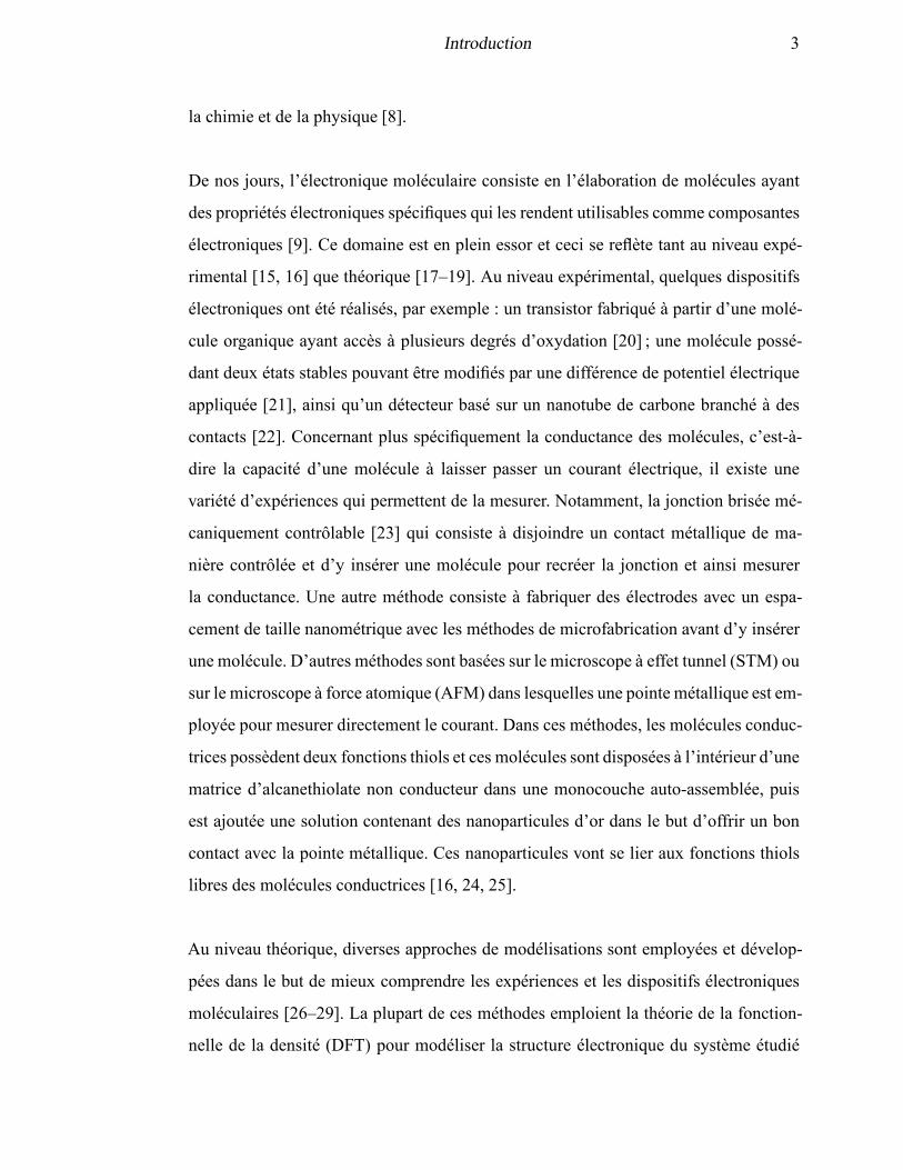
De nos jours, l’électronique moléculaire consiste en l’élaboration de molécules ayant

des propriétés électroniques spécifiques qui les rendent utilisables comme composantes

électroniques [9]. Ce domaine est en plein essor et ceci se reflète tant au niveau expé-

rimental [15, 16] que théorique [17–19]. Au niveau expérimental, quelques dispositifs

électroniques ont été réalisés, par exemple : un transistor fabriqué à partir d’une molé-

cule organique ayant accès à plusieurs degrés d’oxydation [20] ; une molécule possé-

dant deux états stables pouvant être modifiés par une différence de potentiel électrique

appliquée [21], ainsi qu’un détecteur basé sur un nanotube de carbone branché à des

contacts [22]. Concernant plus spécifiquement la conductance des molécules, c’est-à-

dire la capacité d’une molécule à laisser passer un courant électrique, il existe une

variété d’expériences qui permettent de la mesurer. Notamment, la jonction brisée mé-

caniquement contrôlable [23] qui consiste à disjoindre un contact métallique de ma-

nière contrôlée et d’y insérer une molécule pour recréer la jonction et ainsi mesurer

la conductance. Une autre méthode consiste à fabriquer des électrodes avec un espa-

cement de taille nanométrique avec les méthodes de microfabrication avant d’y insérer

une molécule. D’autres méthodes sont basées sur le microscope à effet tunnel (STM) ou

sur le microscope à force atomique (AFM) dans lesquelles une pointe métallique est em-

ployée pour mesurer directement le courant. Dans ces méthodes, les molécules conduc-

trices possèdent deux fonctions thiols et ces molécules sont disposées à l’intérieur d’une

matrice d’alcanethiolate non conducteur dans une monocouche auto-assemblée, puis

est ajoutée une solution contenant des nanoparticules d’or dans le but d’offrir un bon

contact avec la pointe métallique. Ces nanoparticules vont se lier aux fonctions thiols

libres des molécules conductrices [16, 24, 25].

Au niveau théorique, diverses approches de modélisations sont employées et dévelop-

pées dans le but de mieux comprendre les expériences et les dispositifs électroniques

moléculaires [26–29]. La plupart de ces méthodes emploient la théorie de la fonction-

nelle de la densité (DFT) pour modéliser la structure électronique du système étudié

Introduction 4

[30]. Dans la section 1.3.3, nous introduisons les méthodes les plus couramment uti-

lisées pour calculer la conductance moléculaire telle que la méthode des fonctions de

Green, la méthode de diffusion ainsi que la théorie de la fonctionnelle de la densité

dépendante du temps (TDDFT).

La recherche en électronique moléculaire est vaste et diversifiée [31]. Ceci est dû entre

autres au fait qu’il existe beaucoup de défis [14] tant au niveau expérimental que théo-

rique. Il y a plusieurs difficultés, notamment, celles qui consistent à déterminer la posi-

tion des molécules sur les contacts [32] dans les expériences puisque celle-ci peut jouer

un rôle important dans la probabilité de transmission. Aussi, la géométrie à l’interface

de la molécule et du contact peut modifier les caractéristiques de transport significative-

ment [7, 16, 33–39]. D’autres difficultés concernent les effets de l’environnement [40]

et de la température [41] sur la conductance des molécules, sans oublier les larges fluc-

tuations dans les mesures effectuées expérimentalement [42]. Dans le but de répondre

à ces questions, un important travail a été réalisé pour caractériser la conduction de

fils métalliques de tailles nanométriques [43, 44]. D’autre part, étant donné leur struc-

ture particulière qui permet le transport électronique sur de longues distances, les sys-

tèmes possédant des liaisons π conjuguées [45], dont le graphène [46, 47], sont très

étudiés. Parmi les molécules étudiées dans le domaine, certaines molécules ont fait

l’objet d’études dans les monocouches auto-assemblées [48]. Quelques molécules étu-

diées expérimentalement ont des propriétés rectificatrices [14, 49]. La rectification du

courant peut être obtenue de différente manière, notamment, en changeant la nature

des contacts [50] et en modifiant la conformation de la molécule [51]. Aussi, plusieurs

auteurs se sont intéressés aux interactions entre les électrons et les phonons de la mo-

lécule servant de conducteur [52–55]. D’autres travaux portent sur le transport polarisé

en spin [8, 26, 56–58]. Aussi, un important aspect est l’étude des relations entre la struc-

ture des molécules et la conductance [31, 59, 60]. Ce dernier aspect est d’ailleurs celui

auquel nous nous intéressons particulièrement dans le présent travail.

Introduction 5

1.3 Transport en électronique moléculaire

Avant d’aborder la partie principale de la thèse, il convient de se familiariser avec

les notions du modèle de Hückel présentées à la section 1.3.1 et à celles de la méthode

« source-sink potential » (SSP) présentées à la section 1.3.2. Dans le cadre de notre

étude, un DEM signifie un dispositif électronique moléculaire dont la conductance nous

intéresse. Celle-ci varie selon l’énergie à laquelle l’électron accède au système, c’est-à-

dire que la probabilité de transmission d’un électron dans un DEM dépend de l’énergie

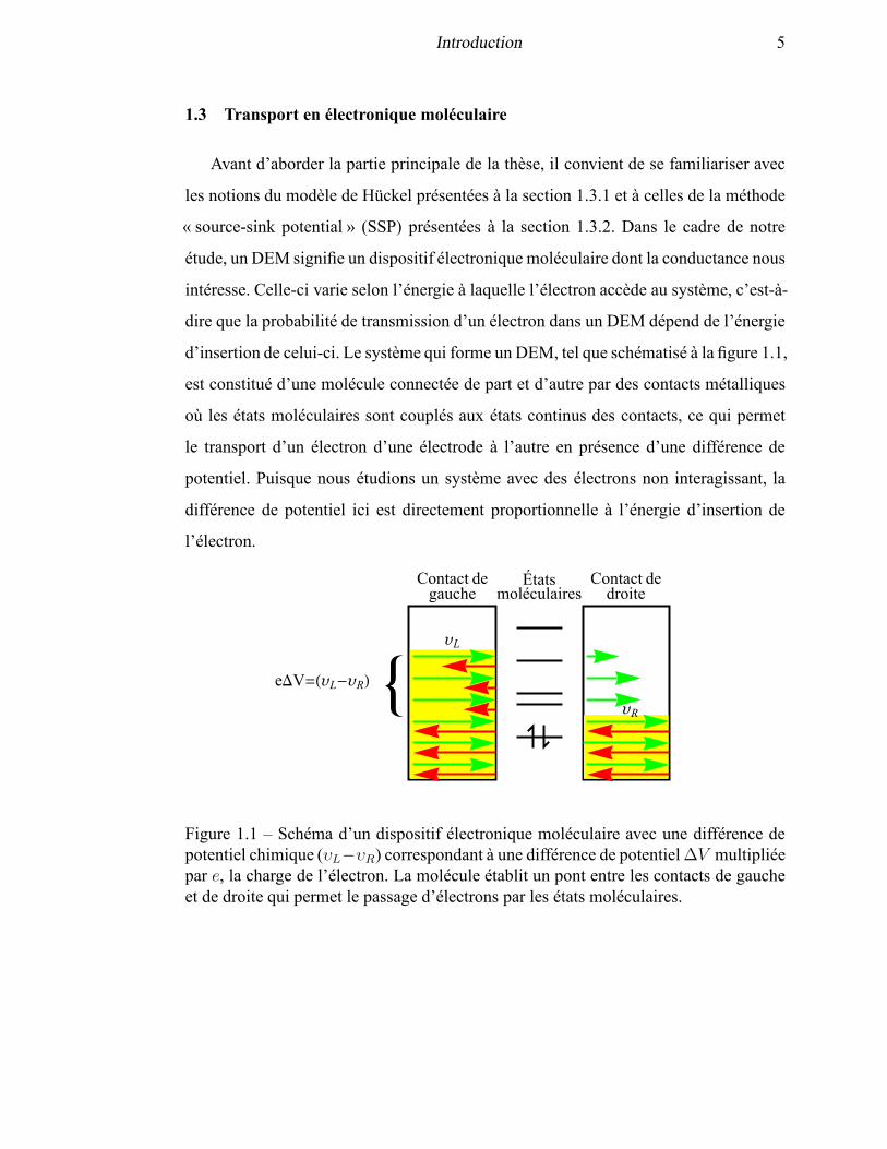
d’insertion de celui-ci. Le système qui forme un DEM, tel que schématisé à la figure 1.1,

est constitué d’une molécule connectée de part et d’autre par des contacts métalliques

où les états moléculaires sont couplés aux états continus des contacts, ce qui permet

le transport d’un électron d’une électrode à l’autre en présence d’une différence de

potentiel. Puisque nous étudions un système avec des électrons non interagissant, la

différence de potentiel ici est directement proportionnelle à l’énergie d’insertion de

l’électron.

Étatsmoléculaires

Contact degauche

Contact dedroite

ΥL

ΥR

eDV=HΥL-ΥRL 8

Figure 1.1 – Schéma d’un dispositif électronique moléculaire avec une différence depotentiel chimique (υL−υR) correspondant à une différence de potentiel∆V multipliéepar e, la charge de l’électron. La molécule établit un pont entre les contacts de gaucheet de droite qui permet le passage d’électrons par les états moléculaires.

Introduction 6

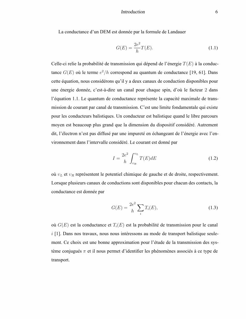
La conductance d’un DEM est donnée par la formule de Landauer

G(E) =2e2

hT (E). (1.1)

Celle-ci relie la probabilité de transmission qui dépend de l’énergie T (E) à la conduc-

tance G(E) où le terme e2/h correspond au quantum de conductance [19, 61]. Dans

cette équation, nous considérons qu’il y a deux canaux de conduction disponibles pour

une énergie donnée, c’est-à-dire un canal pour chaque spin, d’où le facteur 2 dans

l’équation 1.1. Le quantum de conductance représente la capacité maximale de trans-

mission de courant par canal de transmission. C’est une limite fondamentale qui existe

pour les conducteurs balistiques. Un conducteur est balistique quand le libre parcours

moyen est beaucoup plus grand que la dimension du dispositif considéré. Autrement

dit, l’électron n’est pas diffusé par une impureté en échangeant de l’énergie avec l’en-

vironnement dans l’intervalle considéré. Le courant est donné par

I =2e2

h

∫ υL

υR

T (E)dE (1.2)

où υL et υR représentent le potentiel chimique de gauche et de droite, respectivement.

Lorsque plusieurs canaux de conductions sont disponibles pour chacun des contacts, la

conductance est donnée par

G(E) =2e2

h

∑

i

Ti(E), (1.3)

où G(E) est la conductance et Ti(E) est la probabilité de transmission pour le canal

i [1]. Dans nos travaux, nous nous intéressons au mode de transport balistique seule-

ment. Ce choix est une bonne approximation pour l’étude de la transmission des sys-

tème conjugués π et il nous permet d’identifier les phénomènes associés à ce type de

transport.

Introduction 7

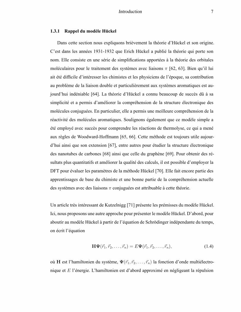
1.3.1 Rappel du modèle Hückel

Dans cette section nous expliquons brièvement la théorie d’Hückel et son origine.

C’est dans les années 1931-1932 que Erich Hückel a publié la théorie qui porte son

nom. Elle consiste en une série de simplifications apportées à la théorie des orbitales

moléculaires pour le traitement des systèmes avec liaisons π [62, 63]. Bien qu’il lui

ait été difficile d’intéresser les chimistes et les physiciens de l’époque, sa contribution

au problème de la liaison double et particulièrement aux systèmes aromatiques est au-

jourd’hui indéniable [64]. La théorie d’Hückel a connu beaucoup de succès dû à sa

simplicité et a permis d’améliorer la compréhension de la structure électronique des

molécules conjuguées. En particulier, elle a permis une meilleure compréhension de la

réactivité des molécules aromatiques. Soulignons également que ce modèle simple a

été employé avec succès pour comprendre les réactions de thermolyse, ce qui a mené

aux règles de Woodward-Hoffmann [65, 66]. Cette méthode est toujours utile aujour-

d’hui ainsi que son extension [67], entre autres pour étudier la structure électronique

des nanotubes de carbones [68] ainsi que celle du graphène [69]. Pour obtenir des ré-

sultats plus quantitatifs et améliorer la qualité des calculs, il est possible d’employer la

DFT pour évaluer les paramètres de la méthode Hückel [70]. Elle fait encore partie des

apprentissages de base du chimiste et une bonne partie de la compréhension actuelle

des systèmes avec des liaisons π conjuguées est attribuable à cette théorie.

Un article très intéressant de Kutzelnigg [71] présente les prémisses du modèle Hückel.

Ici, nous proposons une autre approche pour présenter le modèle Hückel. D’abord, pour

aboutir au modèle Hückel à partir de l’équation de Schrödinger indépendante du temps,

on écrit l’équation

HΨ(~r1, ~r2, . . . , ~rn) = EΨ(~r1, ~r2, . . . , ~rn), (1.4)

où H est l’hamiltonien du système, Ψ(~r1, ~r2, . . . , ~rn) la fonction d’onde multiélectro-

nique et E l’énergie. L’hamiltonien est d’abord approximé en négligeant la répulsion

Introduction 8

entre les électrons, ce qui nous permet d’écrire

H =

n∑

j=1

Hj. (1.5)

Cette opération simplifie grandement le problème puisque la fonction d’onde multi-

électronique Ψ(~r1, ~r2, . . . , ~rn) devient un produit des fonctions d’onde qui sont les so-

lutions des hamiltoniensHj . Il y a autant d’hamiltoniensHj qu’il y a d’électrons et par

conséquent, il y a n orbitales moléculaires. Ces solutions sont écrites Ψj(~ri), où j est

l’indice qui distingue les différentes solutions de Hj et i indique quel électron occupe

l’orbitale moléculaire Ψj . La fonction d’onde multiélectronique est donc approximée

par un déterminant de Slater

Ψ(~r1, ~r2, . . . , ~rn) =1√n!det(Ψ1(~r1)Ψ2(~r2) . . .Ψn(~rn)), (1.6)

où chaque orbitale moléculaire est exprimée par une combinaison linéaire d’orbitales

atomiques

Ψj =n

∑

k=1

cjkφk. (1.7)

Ici, nous avons enlevé l’indice pour l’électron pour plus de clarté. Les coefficients cjk

représentent l’amplitude de l’orbitale atomique φk présente dans la fonction d’onde mo-

léculaire Ψj . Ici, le nombre d’orbitales atomiques correspond au nombre d’électrons

considérés, puisque nous avons un électron par orbitale atomique. En insérant la défini-

tion de la fonction d’onde 1.7 dans l’équation de Schrödinger pour un hamiltonien à un

électronHj particulier et en multipliant par φm à gauche, nous obtenons

Hmk

c1

c2...

cn

= E

Smk

c1

c2...

cn

, (1.8)

où Hmk est l’élément 〈φm|H|φk〉 de l’hamiltonien, E est l’énergie de l’électron dans

l’orbitale moléculaire et Smk est l’intégrale de recouvrement entre l’orbitale atomique

Introduction 9

φm et φk. Les coefficients ck, où k varie de 1 à n, sont regroupés sous la forme d’un

vecteur de taille n. Dans le cadre de l’approximation Hückel, seulement quelques inté-

grales sont non nulles. Ces intégrales sont

〈φm|HHückel|φm〉 = α, (1.9)

〈φm|HHückel|φk〉 =

β si les atomesm et k sont liés,

0 si les atomesm et k ne sont pas liés,(1.10)

Smk = 〈φm|φk〉 =

0 pourm 6= k,

1 pourm = k.(1.11)

Le paramètre α correspond à la valeur de l’énergie d’un électron situé sur l’atome

isolé tandis que β, la valeur de l’intégrale de liaison, décrit le gain d’énergie pour un

électron qui forme la liaison interatomique, c’est-à-dire la liaison π. Dans l’ensemble

de notre travail, nous utilisons des orbitales orthonormées, ce qui a pour conséquence

d’éliminer le terme S de l’équation 1.8, puisqu’il équivaut à la matrice identité I de

dimension n. Ces diverses approximations sont justifiées par le succès de la méthode

Hückel. Celle-ci a toutefois des limites qui sont principalement dues au fait de ne pas

traiter explicitement l’interaction entre les électrons en plus de limiter l’étude aux mo-

lécules planes puisque le modèle Hückel considère seulement les électrons dans les

orbitales atomiques p. Autrement dit, la méthode Hückel néglige les électrons dans les

liaisons de type σ ainsi que les électrons de coeur. Notons que dans ce modèle, on peut

considérer que l’interaction électronique est incluse dans les paramètres α et β. Cette

méthode sert surtout à des comparaisons qualitatives lors d’études sur une série de mo-

lécules semblables, lorsque les paramètres sont calibrés avec l’expérience [62, 72, 73].

Des développements subséquents de l’approche Hückel permettent toutefois de traiter

les molécules non planaires [67].

Introduction 10

Pour une molécule comme le benzène (C6H6) par exemple, la matrice Hückel s’écrit

Hbenzène =

0 β 0 0 0 β

β 0 β 0 0 0

0 β 0 β 0 0

0 0 β 0 β 0

0 0 0 β 0 β

β 0 0 0 β 0

, (1.12)

où α = 0. Une telle valeur de α implique qu’aucun potentiel externe n’est appliqué sur

les atomes. Dans le cas où un hétéroatome serait présent tel que le souffre ou l’azote, il

sert à distinguer la puissance attractive de ces noyaux par rapport au carbone. Comme

les systèmes étudiés ici sont composés exclusivement de carbone, nous choisissons

α = 0 pour tous les atomes. Dans un calcul de la transmission tel que présenté dans

la section 1.3.2, un paramètre α 6= 0 influerait seulement la position de la courbe de

transmission sur l’axe de l’énergie (abscisse). Celle-ci serait simplement déplacée sans

que sa forme soit altérée [74]. Comme nous nous intéressons à la forme qualitative de

celle-ci, ce choix pour la valeur du paramètre α est justifié.

1.3.2 Méthode source-sink potential (SSP) pour le calcul de la conductance

La méthode SSP est développée dans l’optique de faciliter l’établissement de lien

entre la structure et la transmission et ainsi aider les chimistes à employer leurs connais-

sances de la chimie pour prédire la transmission des molécules à l’aide des relations

qu’elle permet de dégager. Elle se distingue des autres méthodologies pour le calcul de

la transmission (section 1.3.3), notamment en fournissant une alternative rigoureuse en

plus d’offrir un autre point de vue dans l’étude des DEMs. Par exemple, la méthode

SSP peut employer les outils déjà disponibles comme la DFT sur une base théorique ri-

goureuse. De plus, elle emploie la notion d’orbitale moléculaire afin de préserver autant

que possible l’aspect visuel du modèle pour expliquer la transmission. Ceci peut être

d’une grande utilité pour simplifier l’éventuel développement de DEMs fonctionnels.

De plus, la méthode SSP est développée par une démarche qui consiste à construire

Introduction 11

un modèle à partir de la base pour ensuite le complexifier graduellement. Cette ma-

nière de faire comporte de nombreux avantages, notamment celui d’avoir un meilleur

contrôle sur le développement en y intégrant des ingrédients qui permettent de traiter

des problèmes de plus en plus complexes et variés. Cet aspect est particulièrement utile

pour identifier l’origine fondamentale d’un phénomène que l’on tente d’expliquer. En

effet, un modèle simple contenant le minimum d’ingrédients pour reproduire un phéno-

mène permet d’identifier l’origine du phénomène par les termes inclus dans le modèle.

De manière générale, différents phénomènes nécessitent divers ingrédients dans l’ha-

miltonien pour se manifester. Par exemple, en tenant compte de l’interaction entre les

électrons, il est possible de reproduire les effets de blocage de Coulomb ou l’effet de

Kondo [75, 76].

HM

HSM

HL HR

ML,SM MSM,R

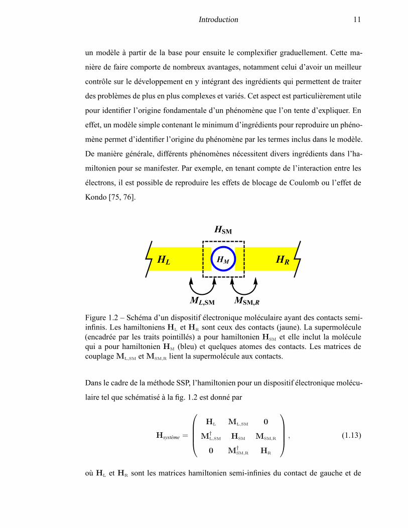
Figure 1.2 – Schéma d’un dispositif électronique moléculaire ayant des contacts semi-infinis. Les hamiltoniens HL et HR sont ceux des contacts (jaune). La supermolécule(encadrée par les traits pointillés) a pour hamiltonien HSM et elle inclut la moléculequi a pour hamiltonien HM (bleu) et quelques atomes des contacts. Les matrices decouplageML,SM etMSM,R lient la supermolécule aux contacts.

Dans le cadre de la méthode SSP, l’hamiltonien pour un dispositif électronique molécu-

laire tel que schématisé à la fig. 1.2 est donné par

Hsystème =

HL ML,SM 0

M†L,SM HSM MSM,R

0 M†SM,R HR

, (1.13)

où HL et HR sont les matrices hamiltonien semi-infinies du contact de gauche et de

Introduction 12

droite, respectivement.ML,SM etM†L,SM couplent la supermolécule au contact de gauche

alors queMR,SM etM†R,SM la couple au contact de droite. La supermolécule contient la

molécule et quelques atomes des contacts adjacents à celle-ci. Ceux-ci sont ajoutés à

la supermolécule jusqu’à ce que la fonction d’onde dans le contact atteigne la forme

asymptotique, c’est-à-dire jusqu’à ce que la fonction d’onde du contact ne change plus

lors de l’ajout d’atomes de contacts supplémentaires. Pour un hamiltonien de type Hü-

ckel, la fonction d’onde prend la forme asymptotique dès le premier atome du contact

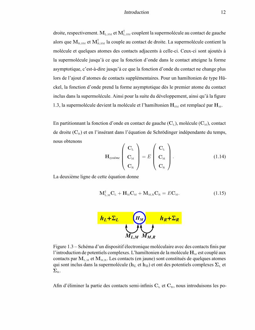
inclus dans la supermolécule. Ainsi pour la suite du développement, ainsi qu’à la figure

1.3, la supermolécule devient la molécule et l’hamiltonienHSM est remplacé parHM.

En partitionnant la fonction d’onde en contact de gauche (CL), molécule (CM), contact

de droite (CR) et en l’insérant dans l’équation de Schrödinger indépendante du temps,

nous obtenons

Hsystème

CL

CM

CR

= E

CL

CM

CR

. (1.14)

La deuxième ligne de cette équation donne

M†L,M

CL +HMCM +MM,RCR = ECM. (1.15)

HMhL+SL hR+SR

ML,M MM ,R

Figure 1.3 – Schéma d’un dispositif électronique moléculaire avec des contacts finis parl’introduction de potentiels complexes. L’hamiltonien de la moléculeHM est couplé auxcontacts parML,M etMM,R. Les contacts (en jaune) sont constitués de quelques atomesqui sont inclus dans la supermolécule (hL et hR) et ont des potentiels complexesΣL etΣR.

Afin d’éliminer la partie des contacts semi-infinis CL et CR, nous introduisons les po-

Introduction 13

tentiels complexesΣL et ΣR (voir fig. 1.3),

M†L,MCL = ΣLCM, (1.16)

et

M†M,R

CR = ΣRCM. (1.17)

Nous pouvons donc remplacer les contacts semi-infinis par des contacts finis à l’aide

des potentiels complexesΣL etΣR dans la mesure où nous connaissons dès le départ les

fonctions d’onde des contactsCL etCR. Autrement dit, les potentiels complexes servent

à reproduire le comportement des fonctions d’onde des contacts à l’infini, c’est-à-dire

à leur limite asymptotique respective. Nous imposons en quelque sorte des conditions

frontières aux deux extrémités du système à l’aide de potentiels complexes. En insérant

les équations 1.16 et 1.17 dans 1.15, cette dernière devient

ΣLCM +HMCM +ΣRCM = ECM. (1.18)

Pour illustrer la méthode SSP, nous allons étudier le cas de l’éthylène branché à gauche

et à droite par des chaînes monoatomiques homogènes semi-infinies qui agissent comme

contacts dans le cadre de l’approximation Hückel. Afin de déterminer les potentiels

complexesΣL et ΣR qui seront ajoutés à la portion moléculaire de l’hamiltonien, nous

devons d’abord découvrir quelles sont les fonctions d’ondes des contacts de gauche et

de droite (voir fig. 1.3). Pour ce faire, nous devons résoudre l’équation séculaire sui-

vante

det (Hcontact − IE) = 0, (1.19)

Introduction 14

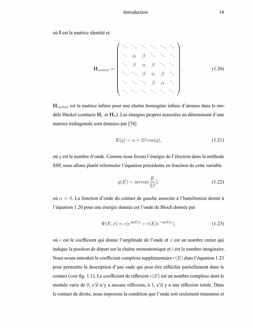
où I est la matrice identité et

Hcontact =

. . . . . . . . . . . . . . . . . .

. . . α β. . . . . . . . .

. . . β α β. . . . . .

. . . . . . β α β. . .

. . . . . . . . . β α. . .

. . . . . . . . . . . . . . . . . .

. (1.20)

Hcontact est la matrice infinie pour une chaîne homogène infinie d’atomes dans le mo-

dèle Hückel (contactsHL etHR). Les énergies propres associées au déterminant d’une

matrice tridiagonale sont données par [74]

E(q) = α+ 2β cos(q), (1.21)

où q est le nombre d’onde. Comme nous fixons l’énergie de l’électron dans la méthode

SSP, nous allons plutôt reformuler l’équation précédente en fonction de cette variable

q(E) = arccos(E

2β), (1.22)

où α = 0. La fonction d’onde du contact de gauche associée à l’hamiltonien donné à

l’équation 1.20 pour une énergie donnée est l’onde de Bloch donnée par

Ψ(E, x) = c(eiq(E)x + r(E)e−iq(E)x), (1.23)

où c est le coefficient qui donne l’amplitude de l’onde et x est un nombre entier qui

indique la position de départ sur la chaîne monoatomique et i est le nombre imaginaire.

Nous avons introduit le coefficient complexe supplémentaire r(E) dans l’équation 1.23

pour permettre la description d’une onde qui peut être réfléchie partiellement dans le

contact (voir fig. 1.1). Le coefficient de réflexion r(E) est un nombre complexe dont le

module varie de 0, s’il n’y a aucune réflexion, à 1, s’il y a une réflexion totale. Dans

le contact de droite, nous imposons la condition que l’onde soit seulement transmise et

Introduction 15

par conséquent, la fonction d’onde du contact s’écrit

Ψ(E, y) = c(eiq(E)y). (1.24)

Pour obtenir le potentiel complexe de gauche ΣL, nous devons résoudre l’équation

suivante

(HL − IE)Ψ = 0, (1.25)

où

HL =

ΣL βL. . . . . .

βL 0 βL. . .

. . . βL 0. . .

. . . . . . . . . . . .

. (1.26)

Nous y arrivons, en insérant la fonction d’onde de l’équation 1.23 dans l’équation

1.25 et nous obtenons après quelques étapes l’équation pour le potentiel complexe de

gauche

ΣL(E) = βLeiqL(E) + r(E)e−iqL(E)

1 + r(E). (1.27)

Pour obtenir l’équation du potentiel complexe de droiteΣR, nous suivons une procédure

analogue et nous obtenons

ΣR(E) = βReiqR(E), (1.28)

où βR est le couplage entre les atomes du contact de droite, qL(E) et qR(E) sont les

nombres d’onde associés à la fonction d’onde des contacts de gauche et de droite, res-

pectivement. Pour l’éthylène, la matrice hamiltonien du système étudié (voir équation

Introduction 16

1.13) a pour éléments

HL = hL + ΣL, (1.29)

ML,M = (βLM 0) , (1.30)

M†L,M =

βLM

0

, (1.31)

HM =

0 βM

βM 0

, (1.32)

MM,R =

0

βRM

, (1.33)

M†M,R = (0 βRM ) , (1.34)

HR = hR + ΣR. (1.35)

Les matrices hL et hR correspondent aux morceaux des contacts inclus dans la super-

molécule, mais comme indiqué auparavant, seulement le premier atome du contact est

nécessaire puisque la fonction d’onde atteint la forme asymptotique dès le départ. Ainsi,

dans l’exemple ici, les matrices hL et hR sont réduites à un seul élément qui vaut 0, soit

la valeur de α. Nous obtenons donc pour l’éthylène

Héthylène =

ΣL βLM 0 0

βLM 0 βM 0

0 βM 0 βRM

0 0 βRM ΣR

, (1.36)

où ΣL et ΣR sont les potentiels complexes de gauche et de droite respectivement,

donnés par les équations 1.27 et 1.28. La transmission du système est donnée par

T (E) = 1 − |r(E)|2, où r(E) est le coefficient de réflexion complexe. Dans le cas

d’une chaîne homogène d’atomes, T = 1 puisque l’électron provenant du contact de

gauche est déjà dans l’état propre de conduction, et ce, peu importe l’énergie choisie

pourvu qu’elle se situe dans les limites permises, c’est-à-dire ±2βL [74].

Introduction 17

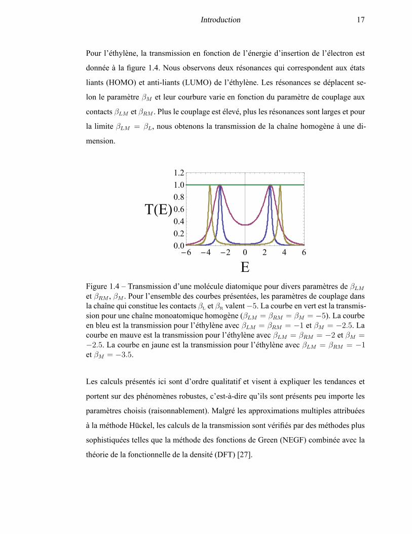
Pour l’éthylène, la transmission en fonction de l’énergie d’insertion de l’électron est

donnée à la figure 1.4. Nous observons deux résonances qui correspondent aux états

liants (HOMO) et anti-liants (LUMO) de l’éthylène. Les résonances se déplacent se-

lon le paramètre βM et leur courbure varie en fonction du paramètre de couplage aux

contacts βLM et βRM . Plus le couplage est élevé, plus les résonances sont larges et pour

la limite βLM = βL, nous obtenons la transmission de la chaîne homogène à une di-

mension.

-6 -4 -2 0 2 4 60.0

0.2

0.4

0.6

0.8

1.0

1.2

E

THEL

Figure 1.4 – Transmission d’une molécule diatomique pour divers paramètres de βLMet βRM , βM . Pour l’ensemble des courbes présentées, les paramètres de couplage dansla chaîne qui constitue les contacts βL et βR valent−5. La courbe en vert est la transmis-sion pour une chaîne monoatomique homogène (βLM = βRM = βM = −5). La courbeen bleu est la transmission pour l’éthylène avec βLM = βRM = −1 et βM = −2.5. Lacourbe en mauve est la transmission pour l’éthylène avec βLM = βRM = −2 et βM =−2.5. La courbe en jaune est la transmission pour l’éthylène avec βLM = βRM = −1et βM = −3.5.

Les calculs présentés ici sont d’ordre qualitatif et visent à expliquer les tendances et

portent sur des phénomènes robustes, c’est-à-dire qu’ils sont présents peu importe les

paramètres choisis (raisonnablement). Malgré les approximations multiples attribuées

à la méthode Hückel, les calculs de la transmission sont vérifiés par des méthodes plus

sophistiquées telles que la méthode des fonctions de Green (NEGF) combinée avec la

théorie de la fonctionnelle de la densité (DFT) [27].

Introduction 18

1.3.3 Autres méthodes de calculs de la conductance

La méthode la plus populaire pour calculer la conductance des DEMs est la mé-

thode des fonctions de Green (NEGF). Nous nous contenterons d’en décrire les idées

principales sans entrer dans les détails. Le principe employé dans cette approche est de

relier une fonction d’onde Ψ(r, t) à une autre Ψ(r′, t′), à une position r′ et à un temps t′

ultérieur à l’aide d’un opérateur [6]. Cet opérateur est formé par les fonctions de Green

et celles-ci donnent l’amplitude de probabilité que la particule décrite par Ψ(r, t) par-

vienne à Ψ(r′, t′). À partir de ces fonctions, nous pouvons comprendre qu’elles sont

directement reliées à la transmission dans un DEM, c’est-à-dire qu’elles contiennent

l’information qui donne la probabilité que la particule provenant du contact de gauche

passe au travers du DEM pour se retrouver dans le contact de droite.

L’équation dérivée pour la transmission selon la méthode NEGF apparaît dans la théo-

rie de la diffusion. Ratner a développé la formule pour la transmission en électronique

moléculaire [27] alors que Seideman et Miller [77] ont dérivé cette formule dans le

contexte de calculs pour la probabilité de réaction. Aussi, Meir et Wingreen [78] ont

étendu la méthode pour inclure l’interaction entre les électrons. L’équation pour la trans-

mission T (E) pour des électrons non interagissant est donnée par

T (E) = Tr(ΓL(E)GR(E)ΓR(E)G

A(E)), (1.37)

où

ΓL(E) = i(ΣRL(E)− (ΣR

L(E))†), (1.38)

et

ΓR(E) = i(ΣRR(E)− (ΣR

R(E))†). (1.39)

GR(E) et GA(E) sont les fonctions de Green retardée et avancée, alors que ΓL(E) et

ΓR(E) représentent le couplage entre la molécule et les contacts de gauche et de droite,

respectivement. Les termes ΣRL(E) et Σ

RR(E) sont les opérateurs de « self-energy » qui

décrivent l’effet du couplage des contacts à la portion moléculaire du système. La mé-

Introduction 19

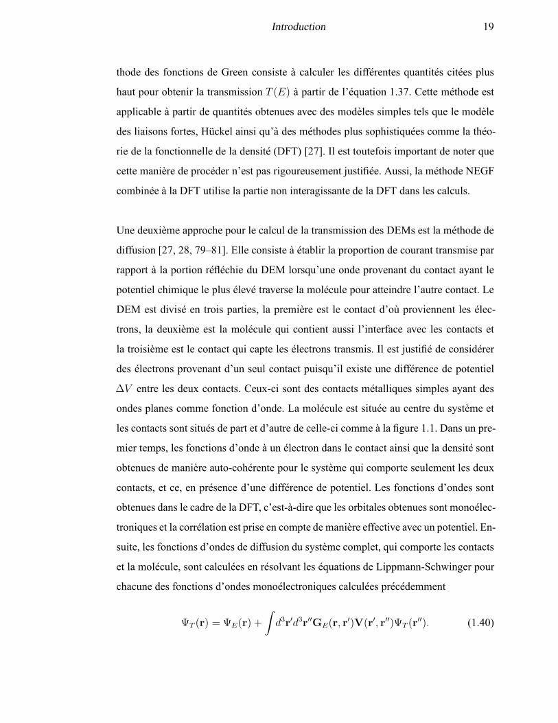
thode des fonctions de Green consiste à calculer les différentes quantités citées plus

haut pour obtenir la transmission T (E) à partir de l’équation 1.37. Cette méthode est

applicable à partir de quantités obtenues avec des modèles simples tels que le modèle

des liaisons fortes, Hückel ainsi qu’à des méthodes plus sophistiquées comme la théo-

rie de la fonctionnelle de la densité (DFT) [27]. Il est toutefois important de noter que

cette manière de procéder n’est pas rigoureusement justifiée. Aussi, la méthode NEGF

combinée à la DFT utilise la partie non interagissante de la DFT dans les calculs.

Une deuxième approche pour le calcul de la transmission des DEMs est la méthode de

diffusion [27, 28, 79–81]. Elle consiste à établir la proportion de courant transmise par

rapport à la portion réfléchie du DEM lorsqu’une onde provenant du contact ayant le

potentiel chimique le plus élevé traverse la molécule pour atteindre l’autre contact. Le

DEM est divisé en trois parties, la première est le contact d’où proviennent les élec-

trons, la deuxième est la molécule qui contient aussi l’interface avec les contacts et

la troisième est le contact qui capte les électrons transmis. Il est justifié de considérer

des électrons provenant d’un seul contact puisqu’il existe une différence de potentiel

∆V entre les deux contacts. Ceux-ci sont des contacts métalliques simples ayant des

ondes planes comme fonction d’onde. La molécule est située au centre du système et

les contacts sont situés de part et d’autre de celle-ci comme à la figure 1.1. Dans un pre-

mier temps, les fonctions d’onde à un électron dans le contact ainsi que la densité sont

obtenues de manière auto-cohérente pour le système qui comporte seulement les deux

contacts, et ce, en présence d’une différence de potentiel. Les fonctions d’ondes sont

obtenues dans le cadre de la DFT, c’est-à-dire que les orbitales obtenues sont monoélec-

troniques et la corrélation est prise en compte de manière effective avec un potentiel. En-

suite, les fonctions d’ondes de diffusion du système complet, qui comporte les contacts

et la molécule, sont calculées en résolvant les équations de Lippmann-Schwinger pour

chacune des fonctions d’ondes monoélectroniques calculées précédemment

ΨT (r) = ΨE(r) +

∫

d3r′d3r′′GE(r, r′)V(r′, r′′)ΨT (r

′′). (1.40)

Introduction 20

ΨT (r) est la fonction d’onde totale du système,ΨE(r) est celle des contacts seulement,

GE(r, r′) est la fonction de Green des contacts etV(r′, r′′) est le potentiel de diffusion.

Ce dernier représente le potentiel perçu par les électrons du contact qui arrive sur la

molécule. Le courant est obtenu en faisant la somme des contributions des états de

diffusion qui sont occupés selon la distribution de Fermi dans les contacts. À partir du

courant J , la transmission est obtenue par

T (E) = Jtransmis(E)/JIncident(E). (1.41)

D’autres auteurs dont Tsukada [82, 83] et Guo [84] ont développé des approches simi-

laires pour le calcul de la conductance d’un DEM.

Une troisième approche utilise la théorie de la fonctionnelle de la densité dépendante

du temps (TDDFT) [85] pour calculer la transmission des DEMs. Il existe deux catégo-

ries d’approche qui emploient la TDDFT pour y parvenir [86]. La première utilise les

fonctions de Green dans le domaine du temps [87–90] pour déterminer le courant alors

que la seconde propage la fonction d’onde dans le temps [91–93]. La seconde méthode

est en principe exacte puisque la densité obtenue change en fonction du temps, ce qui

mène naturellement au calcul du courant [86]. Elle consiste à prendre un DEM à l’équi-

libre et à lui appliquer une perturbation dépendante du temps au niveau des contacts.

Cette perturbation est attribuable à l’application d’une différence de potentiel lors de

l’expérience. Cette méthode a l’avantage de donner la valeur du courant en fonction

du temps, ce qui permet d’étudier l’état transitoire du courant avant qu’il n’y ait sta-

bilisation, contrairement aux approches déjà mentionnées [89, 94]. Ainsi, elle est plus

proche de l’expérience puisque le potentiel est appliqué aux contacts à partir d’un cer-

tain temps t0 [95]. Dans cette approche, la densité électronique en fonction du temps

est calculée à l’aide des orbitales Kohn-Sham du DEM qui sont elles aussi propagées

dans le temps. Cependant, comme la densité calculée provient de la DFT, les effets pro-

venant de la corrélation sont approximés, c’est-à-dire que la fonctionnelle d’échange

et de corrélation n’est pas exacte. De plus, il n’est pas évident que les fonctionnelles

Introduction 21

d’échanges et de corrélation actuellement disponibles s’appliquent aux systèmes hors-

équilibres puisqu’elles ont été dérivées dans des conditions d’équilibre [96]. Un autre

problème potentiel vient du fait que la méthode nécessite la fonctionnelle d’échange et

de corrélation appropriée qui dépend du temps t et qui n’est pas disponible.

1.4 Pertinence des travaux

Pourquoi avons-nous besoin d’une autre méthode pour le calcul de la transmission

des DEMs ? L’idée principale qui guide le développement de la méthode SSP est de

rendre possible l’utilisation d’outils déjà disponibles afin de les utiliser dans le cadre

de l’étude des DEMs, et ce, de manière rigoureuse. Par exemple, nous pouvons adapter

la méthode SSP pour qu’elle fonctionne avec la DFT et ainsi calculer la transmission

en incluant l’interaction entre les électrons de manière effective. Dans ce cas, les outils

tels que les fonctionnelles d’échange et de corrélation sont utilisées dans le contexte du

transport d’électrons. L’approche SSP a également été développée pour faciliter l’iden-

tification de notions pertinentes de la chimie pouvant prédire de manière qualitative

la transmission des DEMs. De cette manière, il peut être envisagé, dans la mesure où

de telles correspondances sont établies, que certaines règles de la chimie déjà connues

comme les effets mésomères soient de bons indicateurs pour prédire la transmission

de DEMs. En commençant à partir d’un modèle plus complet dès le départ, il devient

difficile d’assigner les caractéristiques de conduction aux termes de l’hamiltonien. En

revanche, un tel modèle donne une description plus quantitative et globale du phéno-

mène de transport. Il peut servir de point de référence et de comparaison pour des

calculs plus simples tels que ceux présentés ici. La méthode SSP part d’une description

très simplifiée de DEMs pour découvrir quels ingrédients du modèle sont essentiels à

l’étude de certains phénomènes. Il est particulièrement utile de débuter par des modèles

simples pour ensuite les complexifiés lorsqu’on s’intéresse à établir des liens de causa-

lité. Ceci a de nombreux avantages outre la rapidité des calculs effectués. En effet, le

changement de la transmission en fonction de l’ajout ou le retrait d’un terme de l’ha-

miltonien permet de déterminer les interactions importantes pour la caractérisation du

phénomène de transport. Par exemple, les phénomènes d’interférences abordés aux cha-

Introduction 22

pitres 3 et 4 sont déjà présents dans le modèle Hückel, ce qui laisse présager que cette

caractéristique des DEMs est robuste et répandue. De plus, il devient possible dans cer-

tains cas d’obtenir un résultat analytique plutôt que numérique [97, 98], ce qui donne

une meilleure idée des paramètres importants et la dépendance de la transmission par

rapport à eux. En complexifiant le modèle SSP graduellement, il devient possible d’as-

socier les propriétés conductrices des DEMs à des composantes précises incluses dans

le modèle permettant ainsi une meilleure compréhension du transport dans ces dispo-

sitifs. Par exemple, en traitant la corrélation entre les électrons, il devient possible de

décrire l’effet de Kondo [76, 99, 100] et le blocage de Coulomb [44]. Il est aussi utile

de préciser que de notre point de vue, il n’y a pas de méthode supérieure pour obtenir

la transmission puisque chacune (voir section 1.3.3) apporte un point de vue original à

la compréhension du phénomène de transport dans les DEMs.

1.5 Contenu des chapitres

Chaque chapitre est le fruit d’efforts soutenus et chacun posait des défis particuliers.

Par exemple, au cours d’un projet, il arrive fréquemment que l’approche préconisée

initialement échoue et que de nouvelles idées et stratégies doivent être adoptées pour

résoudre les problèmes rencontrés. Ceci s’est révélé particulièrement vrai pour le tra-

vail présenté au chapitre 6, où le code a dû être réécrit à quelques reprises et beaucoup

d’efforts ont dus être déployés afin d’aboutir à un algorithme convenable. Autrement,

la majorité du temps était consacré à l’élaboration de la théorie, au codage informatique

ainsi qu’à l’interprétation des résultats obtenus.

Au chapitre 2, nous cherchons à savoir dans quelle mesure les fonctionnelles d’échange

et de corrélation de la DFT permettent de décrire l’effet de Kondo observé dans un

DEM expérimental. Cet effet est particulièrement associé à l’interaction entre les élec-

trons et nous étudions à l’aide de la DFT, la transmission d’un point quantique molé-

culaire susceptible de présenter cet effet. Ma contribution dans ce projet est principale-

ment d’avoir identifié une molécule susceptible de manifester l’effet de Kondo en plus

Introduction 23

de vérifier que la charge et le spin étaient localisés sur l’atome de cobalt à l’aide de dif-

férentes méthodes disponibles dans le logiciel GAUSSIAN [101]. J’ai aussi participé à

l’interprétation des résultats et à la rédaction.

Les chapitres 3 et 4 portent sur la question : quelles relations pouvons-nous établir

entre la structure de la molécule qui compose un DEM et sa conductance ? Ces deux

chapitres abordent cette question en ciblant les chaînes de carbone conjuguées dans le

premier cas et les molécules aromatiques dans le deuxième. Toutes deux sont des struc-

tures omniprésentes dans l’étude des DEMs. Mes contributions à ces deux chapitres

sont d’avoir créé des exemples et d’avoir participé de manière importante aux discus-

sions et à l’interprétation des résultats ainsi qu’à la révision des manuscrits avant leur

soumission. J’ai également rédigé la section concernant le champ magnétique généré

par les courants circulaires au chapitre 4.

Au chapitre 5 nous employons la méthode des perturbations avec la méthode SSP pour

répondre à la question : Y a-t-il des propriétés moléculaires qui peuvent nous aider à

prédire la capacité conductrice d’une molécule dans un DEM? J’ai produit et rédigé

l’ensemble du contenu de ce chapitre.

Au chapitre 6, nous cherchons à étendre la méthode SSP à plusieurs canaux de conduc-

tions, ceci dans le but principal d’étendre le domaine d’application de la méthode en

plus de chercher les conséquences de cette modification au problème de la conduction

de DEM. J’ai produit et rédigé l’ensemble du contenu de ce chapitre.

Introduction 24

1.6 Bibliographie

[1] D. K. Ferry and S. M. Goodnick, Transport in Nanostructures, Cambridge

University Press, 1997.

[2] D. Vuillaume, Comptes rendus physique, 9, 78 (2008).

[3] J. Ramsden, Nanotechnology, Elsevier, 2011.

[4] H. Choi and C. C. M. Mody, Social studies of science, 39, 11 (2009).

[5] P. Peercy, Nature, 406, 1023 (2000).

[6] C. Cohen-Tanoudji, B. Diu, and F. Laloë, Mécanique Quantique, Hermann

éditeurs des sciences et des arts, 1998.

[7] J. Heath and M. Ratner, Physics today, 56, 43 (2003).

[8] N. A. Zimbovskaya and M. R. Pederson, Physics reports-review section of phy-

sics letters, 509, 1 (2011).

[9] J. R. Heath, Annual review of materials research, 39, 1 (2009).

[10] H. Song, M. A. Reed, and T. Lee, Advanced materials, 23, 1583 (2011).

[11] J. Del Nero, F. M. de Souza, and R. B. Capaz, Journal of computational and

theoretical nanoscience, 7, 503 (2010).

[12] A. Coskun, J. M. Spruell, G. Barin, W. R. Dichtel, A. H. Flood, Y. Y. Botros

and J. F. Stoddart, Chemical society reviews, 41, 4827 (2012).

[13] H. B. Akkerman and B. de Boer, Journal of physics-condensed matter, 20,

013001 (2008).

[14] A. Aviram and M. Ratner, Chemical physics letters, 29, 277 (1974).

[15] C. Joachim, J. Gimzewski, and A. Aviram, Nature, 408, 541 (2000).

Introduction 25

[16] F. Chen, J. Hihath, Z. Huang, X. Li, and N. Tao, Annual review of physical

chemistry, 58, 535 (2007).

[17] M. Brandbyge, J. Mozos, P. Ordejon, J. Taylor, and K. Stokbro, Physical review

B, 65, 165401 (2002).

[18] M. V., M. Kemp, and M. Ratner, The journal of chemical physics, 101, 6849

(1994).

[19] S. Datta, Electronic Transport in Mesoscopic Systems, Cambridge University

Press, 1995.

[20] S. Kubatkin, A. Danilov, M. Hjort, J. Cornil, J.-L. Brédas, N. Stuhr-Hansen,

P. Hedegard and T. Bjornholm, Nature, 425, 698 (2003).

[21] C. Collier, G. Mattersteig, E. W. Wong, Y. Luo, K. Beverly, J. Sampaio,

F. M. Raymo, J. F. Stoddart and J. R. Heath, Science, 289, 1172 (2000).

[22] A. K. Feldman, M. L. Steigerwald, X. Guo, and C. Nuckolls, Accounts of che-

mical reasearch, 41, 1731 (2008).

[23] M. Reed, C. Zhou, C. Muller, T. Burgin, and J. Tour, Science, 278, 252 (1997).

[24] R. J. Nichols,W. Haiss, S. J. Higgins, E. Leary, S. Martin and D. Bethell Physical

chemistry chemical physics, 12, 2801 (2010).

[25] Y. Selzer and D. L. Allara, Annual review of physical chemistry, 57, 593 (2006).

[26] W. Y. Kim, Y. C. Choi, S. K. Min, Y. Cho, and K. S. Kim, Chemical society

reviews, 38, 2319 (2009).

[27] Y. Xue, S. Datta, and M. Ratner, Chemical physics, 281, 151 (2002).

[28] N. Lang, Physical review B, 52, 5335 (1995).

[29] Y. Liang, Z. YX, R. Chen, H. AMD Note, H. Mizuseki, and K. Y., The journal

of chemical physics, 129, 024901 (2008).

Introduction 26

[30] M. Koentopp, C. Chang, K. Burke, and R. Car, Journal of physics-condensed

matter, 20, 083203 (2008).

[31] S. V. Aradhya and L. Venkataraman, Nature nanotechnology, 8, 399 (2013).

[32] H. Kondo, H. Kino, J. Nara, T. Ozaki, and T. Ohno, Physical review B, 73,

235323 (2006).

[33] S. Yaliraki, M. Kemp, and M. Ratner, Journal of the american chemical society,

121, 3428 (1999).

[34] S. M. Lindsay and M. A. Ratner, Advanced materials, 19, 23 (2007).

[35] X. Li, J. He, J. Hihath, B. Xu, S. M. Lindsay and N. Tao, Journal of the american

chemical society, 128, 2135 (2006).

[36] H. Basch, R. Cohen, and M. Ratner, Nano letters, 5, 1668 (2005).

[37] A. Nitzan and M. Ratner, Science, 300, 1384 (2003).

[38] H. Weber, J. Reichert, F. Weigend, R. Ochs, D. Beckmann, M. Mayor, R. Ahl-

richs and H. v. Löhneysen, Chemical physics, 281, 113 (2002).

[39] M. Di Ventra, S. Pantelides, and N. Lang, Physical review letters, 84, 979 (2000).

[40] Y. Selzer, L. Cai, M. A. Cabassi, Y. Yao, J. M. Tour, T. S. Mayer and D. L. Allara,

Nano letters, 5, 61 (2005).

[41] Y. Selzer, M. Cabassi, T. Mayer, and D. Allara, Nanotechnology, 15, S483

(2004).

[42] M. Ratner, Nature nanotechnology, 8, 378 (2013).

[43] D. Bowler, Journal of physics-condensed matter, 16, R721 (2004).

[44] N. Agrait, A. Yeyati, and J. van Ruitenbeek, Physics reports-review section of

physics letters, 377, 81 (2003).

[45] M. Kiguchi and S. Kaneko, Chemphyschem, 13, 1116 (2012).

Introduction 27

[46] F. Schwierz, Nature nanotechnology, 5, 487 (2010).

[47] W. Pisula, X. Feng, and K. Muellen, Chemistry of materials, 23, 554 (2011).

[48] G. J. Ashwell, K. Moczko, M. Sujka, A. Chwialkowska, L. .R. Hermann High

and D. J. Sandman, Physical chemistry chemical physics, 9, 996 (2007).

[49] R. Liu, S. Ke, W. Yang, and H. Baranger, Journal of chemical physics, 124,

024718 (2006).

[50] J. B. Pan, Z. H. Zhang, K. H. Ding, X. Q. Deng, and C. Guo, Applied physics

letters, 98, 092102 (2011).

[51] A. Troisi and M. Ratner, Nano letters, 4, 591 (2004).

[52] M. Galperin, M. A. Ratner, and A. Nitzan, Journal of physics-condensed matter,

19, 103201 (2007).

[53] M. Galperin, M. A. Ratner, A. Nitzan, and A. Troisi, Science, 319, 1056 (2008).

[54] T. Frederiksen, M. Paulsson, M. Brandbyge, and A.-P. Jauho, Physical review B,

75, 205413 (2007).

[55] J. Hihath and N. Tao, Progress in surface science, 87, 189 (2012).

[56] M. Shiraishi and T. Ikoma, Physica E-low-dimensional systems & nanostruc-

tures, 43, 1295 (2011).

[57] J. ShangDa, K. Goss, C. Cervetti, and L. Bogani, Science China-chemistry, 55,

867 (2012).

[58] A. Rocha, V. M. Garcia-suarez, S. W. Bailey, C. J. Lambert, J. Ferrer and S. San-

vito, Nature materials, 4, 335 (2005).

[59] M. Mayor, H. B. Weber, J. Reichert, M. Elbing, C. von Hänisch, D. Beckmann

and M. Fischer, Angewandte chemie int. Ed., 42, 5834 (2003).

[60] T. Markussen, R. Stadler, and T. K., Nano letters, 10, 4260 (2010).

Introduction 28

[61] Y. Imry and R. Landauer, Reviews of modern physics, 71, S306 (1999).

[62] B. Vidal, Chimie quantique de l’atome à la théorie de Hückel, Masson, 1993.

[63] P. Hiberty and T. A. Nguyen, Introduction à la chimie quantique, Les éditions

de L’école Polytechnique, 2008.

[64] K. Gavroglu and S. Ana, Neither Physics nor Chemistry. A History of Quantum

Chemistry, The MIT Press, 2011.

[65] R. Hoffmann and R. Woodward, Journal of the american chemical society, 87,

2046 (1965).

[66] R. Woodward and R. Hoffmann, Journal of the american chemical society, 87,

395 (1965).

[67] R. Hoffmann, Journal of chemical physics, 39, 1397 (1963).

[68] J.-C. Charlier, X. Blase, and S. Roche, Reviews of modern physics, 79, 677

(2007).

[69] A. H. Castro Neto, F. Guinea, N. M. R. Peres, K. S. Novoselov, and A. K. Geim,

Reviews of modern physics, 81, 109 (2009).

[70] A. Vela and J. Gazquez, Journal of physical chemistry, 92, 5688 (1988).

[71] W. Kutzelnigg, Journal of computational chemistry, 28, 25 (2006).

[72] C. Couslon and H. Longuethiggins, Proceedings of the royal society of london

series A-mathematical and physical sciences, 191, 39 (1947).

[73] C. Couslon and H. Longuethiggins, Proceedings of the royal society of london

series A-mathematical and physical sciences, 192, 16 (1947).

[74] P. W. Atkins and R. S. Friedman, Molecular Quantum Mechanics Third Edition,

Oxford University Press, 1997.

[75] F. Goyer and M. Ernzerhof, Journal of chemical physics, 134, 174101 (2011).

Introduction 29

[76] G. I. Luiz, E. Vernek, L. Deng, K. Ingersent, and E. V. Anda, Physical review B,

87, 075408 (2013).

[77] T. Seideman and W. Miller, Journal of chemical physics, 97, 2499 (1992).

[78] Y. Meir and N. S. Wingreen, Physical review letters, 68, 2512 (1992).

[79] A. Nitzan, Annual review of physical chemistry, 52, 681 (2001).

[80] M. Di Ventra and N. Lang, Physical review B, 65, 045402 (2002).

[81] N. Lang and P. Avouris, Physical review B, 64, 125323 (2001).

[82] K. Hirose and M. Tsukada, Physical review B, 51, 5278 (1995).

[83] K. Hirose and M. Tsukada, Physical review letters, 73, 150 (1994).

[84] C. Wan, J. Mozos, J. Wang, and H. Guo, Physical review B, 55, 13393 (1997).

[85] E. Runge and E. Gross, Physical review letters, 52, 997 (1984).

[86] K. Varga, Physical review B, 83, 195130 (2011).

[87] S.-H. Ke, R. Liu, W. Yang, and H. U. Baranger, Journal of chemical physics,

132, 234105 (2010).

[88] X. Zheng, F. Wang, C. Y. Yam, Y. Mo, and G. Chen, Physical review B, 75,

195127 (2007).

[89] L. Zhang, Y. Xing, and J. Wang, Physical review B, 86, 155438 (2012).

[90] Y. Zhang, S. Chen, and G. Chen, Phys. Rev. B, 87, 085110 (2013).

[91] N. Sai, N. Bushong, R. Hatcher, andM. Di Ventra, Physical reviewB, 75, 115410

(2007).

[92] C.-L. Cheng, J. S. Evans, and T. Van Voorhis, Physical review B, 74, 155112

(2006).

[93] N. Bushong, N. Sai, and M. Di Ventra, Nano letters, 5, 2569 (2005).

Introduction 30

[94] Y.Wang, C. Y. Yam, T. Frauenheim, G. H. Chen, and N. T. A., Chemical physics,

391, 69 (2011).

[95] G. Stefanucci and C. Almbladh, Physical review B, 69, 195318 (2004).

[96] S. Kurth, G. Stefanucci, C. Almbladh, A. Rubio, and E. Gross, Physical review

B, 72, 035308 (2005).

[97] M. Ernzerhof, Journal of chemical physics, 127, 204709 (2007).

[98] D. Mayou, Y. Zhou, and M. Ernzerhof, Journal of physical chemistry C, 117,

7870 (2013).

[99] G. D. Scott and D. Natelson, ACS nano, 4, 3560 (2010).

[100] P. Huang and E. A. Carter, Nano letters, 6, 1146 (2006).

[101] M. J. Frisch, G. W. Trucks, H. B. Schlegel et al., GAUSSIAN 99, Development

Version, Revision 0.9, Gaussian, Inc., Pittsburgh, PA, 1998.

CHAPITRE 2

APPROXIMATE DENSITY FUNCTIONALS

APPLIED TO MOLECULAR QUANTUM DOTS

Min Zhuang, Philippe Rocheleau, and Matthias Ernzerhof

(Département de Chimie, Université de Montréal,

C.P. 6128 Succursale A, Montréal, Québec H3C 3J7, Canada)

Reproduit avec la permission de Min Zhuang, Philippe Rocheleau, and Matthias

Ernzerhof, The Journal of Chemical Physics, Vol. 122, 154705, (2005). Copyright

2005, American Institute of Physics.

Chapitre 2 32

CONTRIBUTION DES COAUTEURS

Cet article porte sur l’application de méthodes de la théorie de la fonctionnelle de

la densité (DFT) et de la méthode des fonctions de Green pour calculer la transmission

électronique d’un point quantique moléculaire. Min Zhuang et Philippe Rocheleau ont

contribué à part égal pour la création de cet article. Philippe Rocheleau a calculé les

propriétés du cobaltocène ainsi que la distribution des charges dans cette molécule alors

que Min Zhuang a calculé la conductance de la molécule avec la méthode des fonctions

de Green. Les tâches d’interpréter les résultats et d’écrire l’article ont été partagées

également par tous les coauteurs. Matthias Ernzerhof a supervisé les travaux, contribué

à l’interprétation des résultats et à la révision du manuscrit.

Chapitre 2 33

ABSTRACT

Recently, molecular quantum dots (MQDs) have been investigated experimentally

and found to exhibit the Kondo effect. The Kondo effect leads to an enhancement

of the zero-voltage conductance. Here, we study a finite cluster model of a MQD by

means of Kohn-Sham density functional theory. Furthermore, employing an implemen-

tation of Landauer’s formula, we calculate the conductance of the dot. We find that the

electronic structure and the molecular conductance depend strongly on the exchange-

correlation functional employed. While the local spin density approximation and the

Perdew-Burke-Ernzerhof (PBE) generalized gradient approximation qualitatively re-

produce certain features of the Kondo effect, PBE hybrid does not. Based on the MQD,

we discuss the limitations of using density functional theory to model molecular elec-

tronic devices.

Chapitre 2 34

2.1 Introduction

Molecular electronic devices are presently studied extensively [1]. The main prop-

erty of interest is the molecular conductance g. In most systems, qualitative features

of g, as a function of the applied voltage, can be understood in terms of an appropri-

ate single-particle picture. While electron correlation has a quantitative effect on the

results obtained, it is usually not at their origin. Recently, however, molecular quantum

dots (MQDs), exhibiting a conductance behavior typical for a system in a Kondo state

[2, 3] have been reported [4, 5]. The Kondo state is solely a consequence of electron

correlation. It causes an increase in the molecular conductance in the limit of zero bias

voltage. We briefly summarize the prerequisites of a MQD for exhibiting the Kondo

effect. The essential ingredient is a localized, singly occupied d or f orbital. Typi-

cally for d or f electrons, electron-electron repulsion is an important factor to consider.

This singly occupied orbital has an energy below the Fermi surface of the adjacent

macroscopic metal contacts and there has to be a certain nonzero coupling between the

localized state and the continuum of contact states. One would expect that the singly

occupied orbital is filled with an electron from the contacts. However, due to the large

on-site electron-electron repulsion, the energy of the doubly occupied localized orbital

is above the Fermi surface. A system that exhibits the described features can be found

in the Kondo state at sufficiently low temperatures. In the Kondo state, the spin of

the localized electron is screened by electrons around the Fermi energy of the contact,

meaning that the contact electrons and the localized electron are singlet coupled [3].

This resembles a chemical bond between the localized electron and the electrons close

to the Fermi edge of the contacts. As a consequence of this bond formation, the spin

moment associated with the localized state is lost. The net charge transfer between con-

tacts and localized state is often small. However, the transfer of spin density between

contact and localized state eliminates the spin polarization completely.

There are many incarnations of the above described Kondo bond. For instance

cobalt atoms that are deposited on gold surfaces [6, 7] exhibit this phenomenon. Here

we are interested in the Kondo bond that forms when cobalt complexes are attached to

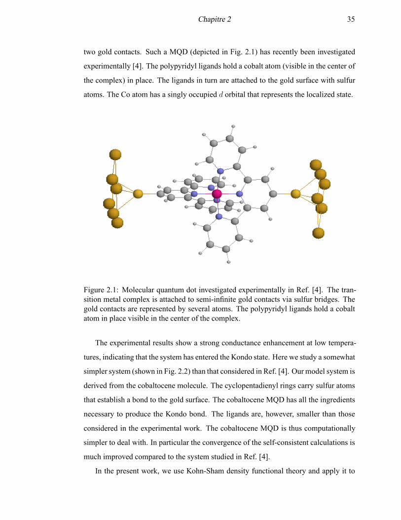
Chapitre 2 35

two gold contacts. Such a MQD (depicted in Fig. 2.1) has recently been investigated

experimentally [4]. The polypyridyl ligands hold a cobalt atom (visible in the center of

the complex) in place. The ligands in turn are attached to the gold surface with sulfur

atoms. The Co atom has a singly occupied d orbital that represents the localized state.

Figure 2.1: Molecular quantum dot investigated experimentally in Ref. [4]. The tran-sition metal complex is attached to semi-infinite gold contacts via sulfur bridges. Thegold contacts are represented by several atoms. The polypyridyl ligands hold a cobaltatom in place visible in the center of the complex.

The experimental results show a strong conductance enhancement at low tempera-

tures, indicating that the system has entered the Kondo state. Here we study a somewhat

simpler system (shown in Fig. 2.2) than that considered in Ref. [4]. Our model system is

derived from the cobaltocene molecule. The cyclopentadienyl rings carry sulfur atoms

that establish a bond to the gold surface. The cobaltocene MQD has all the ingredients

necessary to produce the Kondo bond. The ligands are, however, smaller than those

considered in the experimental work. The cobaltocene MQD is thus computationally

simpler to deal with. In particular the convergence of the self-consistent calculations is

much improved compared to the system studied in Ref. [4].

In the present work, we use Kohn-Sham density functional theory and apply it to

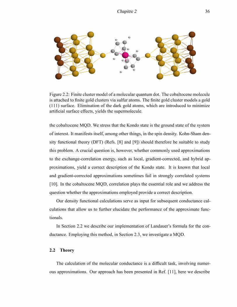
Chapitre 2 36

Figure 2.2: Finite cluster model of a molecular quantum dot. The cobaltocene moleculeis attached to finite gold clusters via sulfur atoms. The finite gold cluster models a gold(111) surface. Elimination of the dark gold atoms, which are introduced to minimizeartificial surface effects, yields the supermolecule.

the cobaltocene MQD. We stress that the Kondo state is the ground state of the system

of interest. It manifests itself, among other things, in the spin density. Kohn-Sham den-

sity functional theory (DFT) (Refs. [8] and [9]) should therefore be suitable to study

this problem. A crucial question is, however, whether commonly used approximations

to the exchange-correlation energy, such as local, gradient-corrected, and hybrid ap-

proximations, yield a correct description of the Kondo state. It is known that local

and gradient-corrected approximations sometimes fail in strongly correlated systems

[10]. In the cobaltocene MQD, correlation plays the essential role and we address the

question whether the approximations employed provide a correct description.

Our density functional calculations serve as input for subsequent conductance cal-

culations that allow us to further elucidate the performance of the approximate func-

tionals.

In Section 2.2 we describe our implementation of Landauer’s formula for the con-

ductance. Employing this method, in Section 2.3, we investigate a MQD.

2.2 Theory

The calculation of the molecular conductance is a difficult task, involving numer-

ous approximations. Our approach has been presented in Ref. [11], here we describe

Chapitre 2 37

it briefly because its details depend on the system at hand. The system consists of a

cobalt complex that is connected to two metal contacts. To simplify the conductance

calculations, the system is divided into two semi-infinite contacts and a remaining su-

permolecule. The supermolecule consists of the molecule and finite clusters of contact

atoms. The semi-infinite contacts are described by Hamiltonian matricesHC (C = L or

R for the left or right contact, respectively). The supermolecule Hamiltonian matrix is

denoted by HM. The coupling matrix connecting HC and HM is given byMCM. For no-

tational simplicity, we assume that the basis functions are orthonormal, thus no overlap

matrices appear in the equations. The zero-voltage conductance can now be obtained

according to [12–15]

g(E) = (2π)2e2

hTr

[

M †RMδ(HR −E)MRMG

r(E)M †LMδ(HL − E)MLMG

a(E)]

,

(2.1)

given that the energy E is set equal to the Fermi energy EF of the system. The term

δ(HC − E) in Eq. 2.1 gives the density of states matrix of the contact C. Gr and Ga

in the same equation denote the retarded and advanced Green’s function of the system,

respectively. Gr and Ga are the most difficult parts of Eq. 2.1 to compute. We employ

single-particle Hamiltonians (i.e., Kohn-Sham- and Hückel Hamiltonians) to simplify

the calculation of the Green’s functions. Furthermore, using the matrix partitioning

technique [14], we introduce an effective supermolecular Hamiltonian matrixHeff ,

Heff(E) = HM − ΣL(E)− ΣR(E), (2.2)

whereΣL(E) andΣR(E) are the self-energy matrices of the semi-infinite contacts, i.e.,

ΣC (E) =M †CM

1

HC − E + i ηMCM . (2.3)

Note that the eigenvalues of Heff are identical to those of the total Hamiltonian matrix

of the MED. The contribution MCMGr/a(E)M †

C′M , needed to evaluate Eq. 2.1, can

Chapitre 2 38

be expressed in terms of Heff (Refs. [14] and [15]),

MCMGr/a(E)M †

C′M =MCM1

Heff(E)− E −+ i η

M †C′M . (2.4)

For the retarded Green’s function, the infinitesimal imaginary part iη has a negative

sign, whereas the positive sign is taken for the advanced Green’s function. To obtain

the supermolecular HamiltonianHM in Eq. 2.2, we use the self-consistent Kohn-Sham

matrix of a calculation considering the supermolecule plus additional contact atoms

attached to the supermolecule. For an illustration, we refer to Fig. 2.2. The light gold

atoms belong to the supermolecule while the dark ones represent a surface layer that

is removed later, i.e., after self-consistency is achieved, we eliminate all but the matrix

elements of the supermolecule from the Kohn-Sham matrix to obtainHM.

To get the Hamiltonian HC of the semi-infinite contacts, we have to resort to a

simple self-consistent spd tight-binding method [16–18]. In the separate calculations

for the contacts, we in turn include parts of the supermolecule. For an illustration we

refer to Fig. 2.3. Our gold contacts consist of a supercell of dimension 14 × 15 ×45 Å

3containing two big slabs separated by a gap of about 17 Å. For simplicity, we

only consider the Γ point in the periodic boundary condition calculation. The matrix

elements of the resulting tight-binding Hamiltonian that correspond to the dark atoms

in Fig. 2.3 are discarded to yield HC. The coupling matrix between the light and dark

atoms in Fig. 2.3 yields MCM . We use an iterative method [19, 20] to construct the

surface Green’s function of a system that is semi-infinite perpendicular to its surface.

This surface Green’s function is then employed to calculate the self-energy matrices of

the contacts in Eq. 2.3.

The Kohn-Sham calculations for the supermolecule are performed with the GAUS-

SIAN [21]. For the gold atoms, we use an spd valence orbital basis set with a corre-

sponding pseudopotential [22] to ensure compatibility with the tight-binding Hamilto-

nian. The 6-31G* basis set is employed for the remaining atoms.

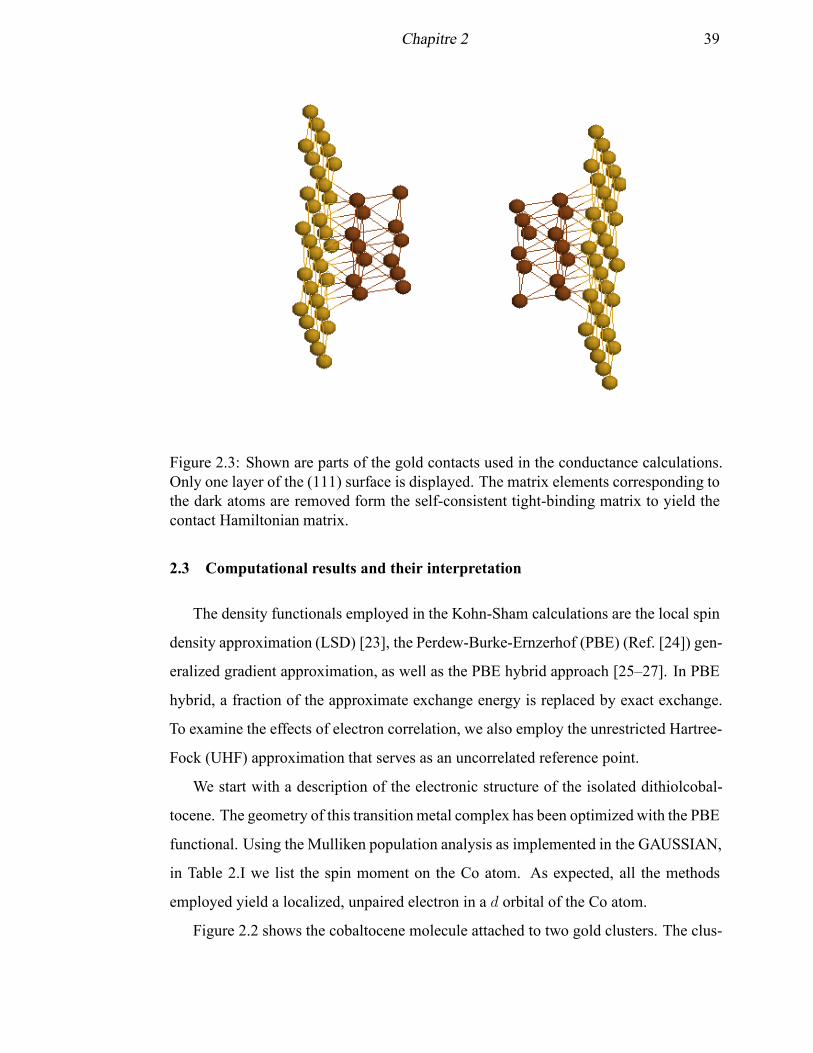
Chapitre 2 39

Figure 2.3: Shown are parts of the gold contacts used in the conductance calculations.Only one layer of the (111) surface is displayed. The matrix elements corresponding tothe dark atoms are removed form the self-consistent tight-binding matrix to yield thecontact Hamiltonian matrix.

2.3 Computational results and their interpretation

The density functionals employed in the Kohn-Sham calculations are the local spin

density approximation (LSD) [23], the Perdew-Burke-Ernzerhof (PBE) (Ref. [24]) gen-

eralized gradient approximation, as well as the PBE hybrid approach [25–27]. In PBE

hybrid, a fraction of the approximate exchange energy is replaced by exact exchange.

To examine the effects of electron correlation, we also employ the unrestricted Hartree-

Fock (UHF) approximation that serves as an uncorrelated reference point.

We start with a description of the electronic structure of the isolated dithiolcobal-

tocene. The geometry of this transitionmetal complex has been optimized with the PBE

functional. Using the Mulliken population analysis as implemented in the GAUSSIAN,

in Table 2.I we list the spin moment on the Co atom. As expected, all the methods

employed yield a localized, unpaired electron in a d orbital of the Co atom.

Figure 2.2 shows the cobaltocene molecule attached to two gold clusters. The clus-

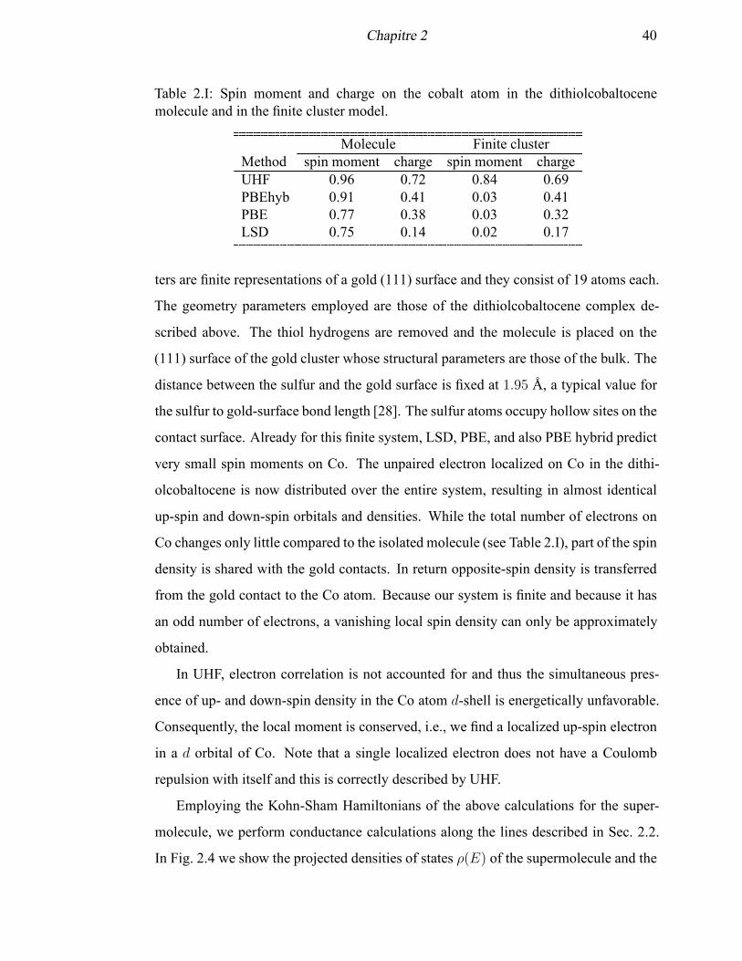
Chapitre 2 40

Table 2.I: Spin moment and charge on the cobalt atom in the dithiolcobaltocenemolecule and in the finite cluster model.

Molecule Finite clusterMethod spin moment charge spin moment chargeUHF 0.96 0.72 0.84 0.69PBEhyb 0.91 0.41 0.03 0.41PBE 0.77 0.38 0.03 0.32LSD 0.75 0.14 0.02 0.17

ters are finite representations of a gold (111) surface and they consist of 19 atoms each.

The geometry parameters employed are those of the dithiolcobaltocene complex de-

scribed above. The thiol hydrogens are removed and the molecule is placed on the

(111) surface of the gold cluster whose structural parameters are those of the bulk. The

distance between the sulfur and the gold surface is fixed at 1.95 Å, a typical value for

the sulfur to gold-surface bond length [28]. The sulfur atoms occupy hollow sites on the

contact surface. Already for this finite system, LSD, PBE, and also PBE hybrid predict

very small spin moments on Co. The unpaired electron localized on Co in the dithi-

olcobaltocene is now distributed over the entire system, resulting in almost identical

up-spin and down-spin orbitals and densities. While the total number of electrons on

Co changes only little compared to the isolated molecule (see Table 2.I), part of the spin

density is shared with the gold contacts. In return opposite-spin density is transferred

from the gold contact to the Co atom. Because our system is finite and because it has

an odd number of electrons, a vanishing local spin density can only be approximately

obtained.

In UHF, electron correlation is not accounted for and thus the simultaneous pres-

ence of up- and down-spin density in the Co atom d-shell is energetically unfavorable.

Consequently, the local moment is conserved, i.e., we find a localized up-spin electron

in a d orbital of Co. Note that a single localized electron does not have a Coulomb

repulsion with itself and this is correctly described by UHF.

Employing the Kohn-Sham Hamiltonians of the above calculations for the super-

molecule, we perform conductance calculations along the lines described in Sec. 2.2.

In Fig. 2.4 we show the projected densities of states ρ(E) of the supermolecule and the

Chapitre 2 41

transmission probabilities T (E) obtained with the various methods. T (E) is related to

the conductance by g(E) = G0T (E) with G0 = 2e2/h. In the UHF calculations for

the finite cluster model there is no bond formation at all between the localized electron

on Co and the gold contacts. Consequently, ρ(E) is flat at the Fermi energy and T (E)

is close to zero. Furthermore up- and down-spin curves are quite different due to the

localized electron that introduces a considerable spin polarization. In the PBE and LSD

calculations, we observe a strong increase in ρ(E) at the Fermi energy, indicating the

formation of a bond between Co and the gold contacts. In accordance with this inter-

pretation, for PBE and LSD we find transmission probabilities approaching one (for

the sum of the up- and down-spin channel), i.e., the complex becomes transparent for

electrons. The localized moment is lost in PBE and LSD. Therefore, up- and down-spin

curves are almost identical. The Kondo temperature is sometimes estimated from the

width of the peak in ρ(E) at half height. For the LSD and PBE calculations such an

estimate yields a Kondo temperature of about 110 K.

A somewhat unexpected picture emerges for the PBE hybrid calculations. The

localized spin moment is lost. However, the conductance at the Fermi energy is very

small. A possible interpretation of this result is that the delocalized orbitals that yield

the large conductance in LSD and PBE are shifted up in energy. Comparison of ρ(E)

and of T (E) between LSD, PBE, and PBE hyrbid supports this idea. There are peaks

in ρ(E) and in T (E) above the Fermi energy for PBE hybrid that resemble the ones

observed for LSD and PBE at the Fermi energy. In PBE hybrid, the localized moment

of the cobaltocene molecule is distributed over the entire system by means of orbitals

that are not at the Fermi energy. We should mention that, following the general practice

[27], in the PBE hybrid calculations the energy is minimized with respect to the orbitals

instead of the density. Thus, the one particle potential in the self-consistent equations

contains a fraction of the Hartree-Fock nonlocal exchange potential. This might cause

the observed differences between PBE and PBE hybrid since Hartree-Fock opens up

the HOMO-LUMO gap in comparison to PBE and LSD.

The question arises how to interpret these results that differ dramatically in their

physical implications. Before discussing this issue, we describe the mechanism by

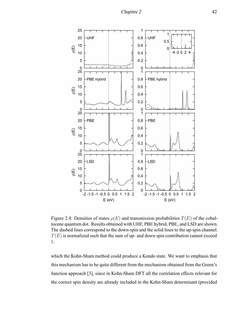
Chapitre 2 42

0

5

10

15

20

25

-2 -1.5 -1 -0.5 0 0.5 1 1.5 2

ρ(E

)

E (eV)

LSD

0

0.2

0.4

0.6

0.8

1

-2 -1.5 -1 -0.5 0 0.5 1 1.5 2

E (eV)

LSD

0

5

10

15

20

25

ρ(E

)

PBE

0

0.2

0.4

0.6

0.8

1

PBE

0

5

10

15

20

25ρ(E

)

PBE hybrid

0

0.2

0.4

0.6

0.8

1

PBE hybrid

0

5

10

15

20

25

ρ(E

)

UHF

0

0.2

0.4

0.6

0.8

1

UHF

0

0.5

1

-4 -2 0 2 4

Figure 2.4: Densities of states ρ(E) and transmission probabilities T (E) of the cobal-tocene quantum dot. Results obtained with UHF, PBE hybrid, PBE, and LSD are shown.The dashed lines correspond to the down-spin and the solid lines to the up-spin channel.T (E) is normalized such that the sum of up- and down spin contribution cannot exceed1.

which the Kohn-Sham method could produce a Kondo state. We want to emphasis that

this mechanism has to be quite different from the mechanism obtained from the Green’s

function approach [3], since in Kohn-Sham DFT all the correlation effects relevant for

the correct spin density are already included in the Kohn-Sham determinant (provided

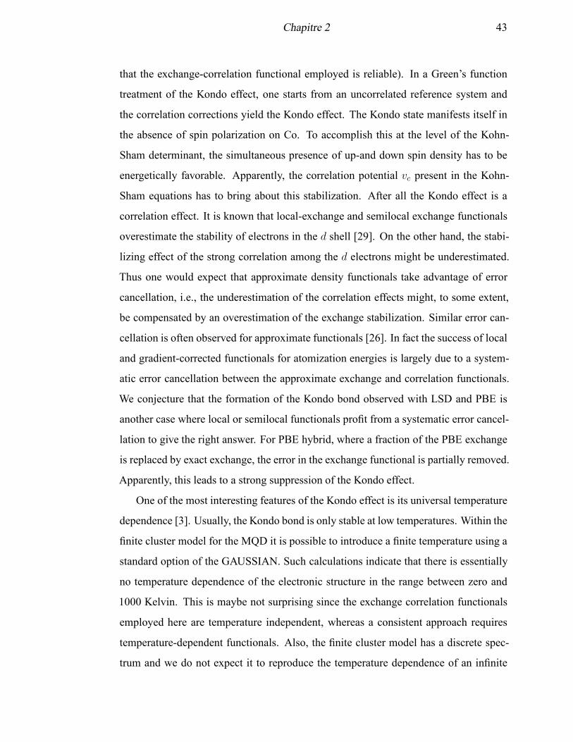
Chapitre 2 43

that the exchange-correlation functional employed is reliable). In a Green’s function

treatment of the Kondo effect, one starts from an uncorrelated reference system and

the correlation corrections yield the Kondo effect. The Kondo state manifests itself in

the absence of spin polarization on Co. To accomplish this at the level of the Kohn-

Sham determinant, the simultaneous presence of up-and down spin density has to be

energetically favorable. Apparently, the correlation potential vc present in the Kohn-

Sham equations has to bring about this stabilization. After all the Kondo effect is a

correlation effect. It is known that local-exchange and semilocal exchange functionals

overestimate the stability of electrons in the d shell [29]. On the other hand, the stabi-

lizing effect of the strong correlation among the d electrons might be underestimated.

Thus one would expect that approximate density functionals take advantage of error

cancellation, i.e., the underestimation of the correlation effects might, to some extent,

be compensated by an overestimation of the exchange stabilization. Similar error can-

cellation is often observed for approximate functionals [26]. In fact the success of local

and gradient-corrected functionals for atomization energies is largely due to a system-

atic error cancellation between the approximate exchange and correlation functionals.

We conjecture that the formation of the Kondo bond observed with LSD and PBE is

another case where local or semilocal functionals profit from a systematic error cancel-

lation to give the right answer. For PBE hybrid, where a fraction of the PBE exchange

is replaced by exact exchange, the error in the exchange functional is partially removed.

Apparently, this leads to a strong suppression of the Kondo effect.

One of the most interesting features of the Kondo effect is its universal temperature

dependence [3]. Usually, the Kondo bond is only stable at low temperatures. Within the

finite cluster model for the MQD it is possible to introduce a finite temperature using a

standard option of the GAUSSIAN. Such calculations indicate that there is essentially

no temperature dependence of the electronic structure in the range between zero and

1000 Kelvin. This is maybe not surprising since the exchange correlation functionals

employed here are temperature independent, whereas a consistent approach requires

temperature-dependent functionals. Also, the finite cluster model has a discrete spec-

trum and we do not expect it to reproduce the temperature dependence of an infinite

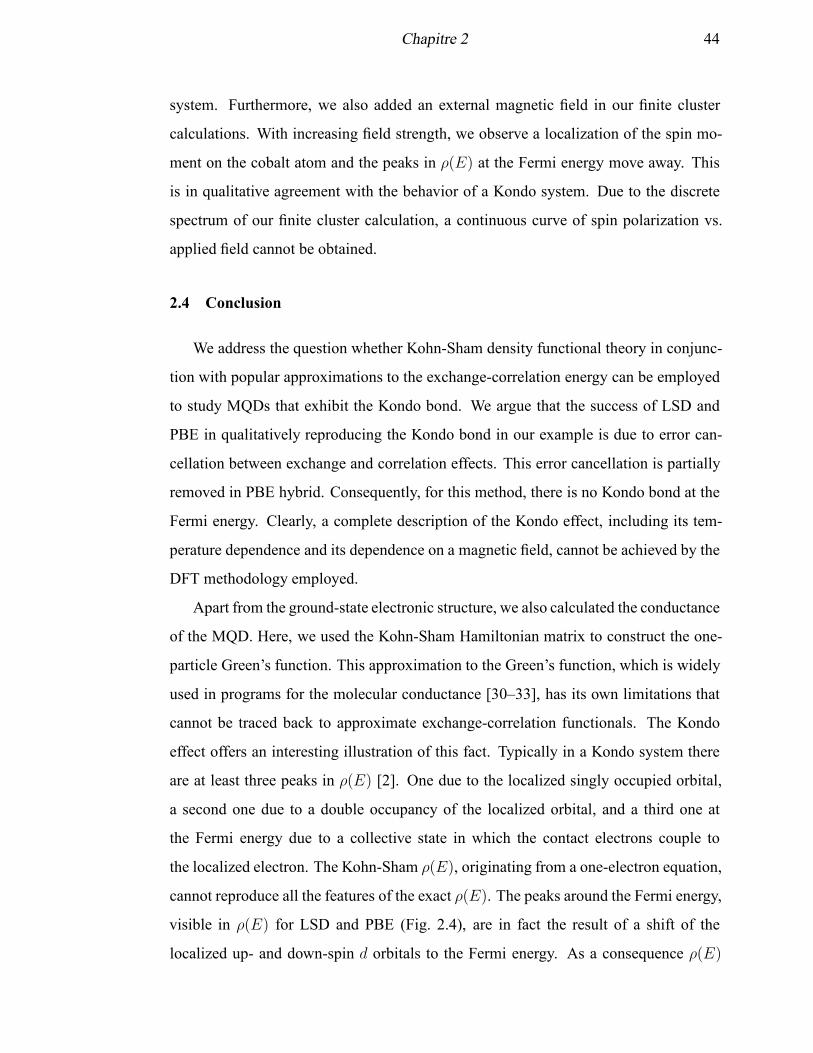
Chapitre 2 44

system. Furthermore, we also added an external magnetic field in our finite cluster

calculations. With increasing field strength, we observe a localization of the spin mo-

ment on the cobalt atom and the peaks in ρ(E) at the Fermi energy move away. This

is in qualitative agreement with the behavior of a Kondo system. Due to the discrete

spectrum of our finite cluster calculation, a continuous curve of spin polarization vs.

applied field cannot be obtained.

2.4 Conclusion

We address the question whether Kohn-Sham density functional theory in conjunc-

tion with popular approximations to the exchange-correlation energy can be employed

to study MQDs that exhibit the Kondo bond. We argue that the success of LSD and

PBE in qualitatively reproducing the Kondo bond in our example is due to error can-

cellation between exchange and correlation effects. This error cancellation is partially

removed in PBE hybrid. Consequently, for this method, there is no Kondo bond at the

Fermi energy. Clearly, a complete description of the Kondo effect, including its tem-

perature dependence and its dependence on a magnetic field, cannot be achieved by the

DFT methodology employed.

Apart from the ground-state electronic structure, we also calculated the conductance

of the MQD. Here, we used the Kohn-Sham Hamiltonian matrix to construct the one-

particle Green’s function. This approximation to the Green’s function, which is widely

used in programs for the molecular conductance [30–33], has its own limitations that

cannot be traced back to approximate exchange-correlation functionals. The Kondo

effect offers an interesting illustration of this fact. Typically in a Kondo system there

are at least three peaks in ρ(E) [2]. One due to the localized singly occupied orbital,

a second one due to a double occupancy of the localized orbital, and a third one at

the Fermi energy due to a collective state in which the contact electrons couple to

the localized electron. The Kohn-Sham ρ(E), originating from a one-electron equation,

cannot reproduce all the features of the exact ρ(E). The peaks around the Fermi energy,

visible in ρ(E) for LSD and PBE (Fig. 2.4), are in fact the result of a shift of the

localized up- and down-spin d orbitals to the Fermi energy. As a consequence ρ(E)

Chapitre 2 45

obtained from a Kohn-Sham Green’s function is missing two of the three peaks typical

for the Kondo system. However, at the Fermi energy, we believe that we obtain a

qualitatively correct description. This claim is supported by the fact that in the exact

theory the highest Kohn-Sham orbital energy equals minus the ionization potential [8].

In approximate DFT the validity of this theorem requires accurate functionals.

Summarizing, we find that with local and semilocal functionals we can qualitatively

describe certain features of the Kondo bond in the cobaltocene MQD. A satisfactory

description of the Kondo effect requires, however, a true many-particle approach to

the one-particle Green’s function. Similarly, an accurate description of the molecular

conductance for strongly correlated systems cannot be achieved with the Kohn-Sham

Green’s function.

Acknowledgements

M.E. would like to acknowledge enlightening discussions with D. C. Langreth. Fur-

thermore, the authors are thankful for the financial support provided byNSERC through

grant 238404-03.

Chapitre 2 46

2.5 Bibliography

[1] A. Nitzan and M. A. Ratner, Nature (London) 300, 1384 (2003).

[2] L. Kouwenhoven and L. Glazman, Phys. World 14(1) 33 (2001).

[3] G. D. Mahan, Many-Particle Physics (Plenum, New York, 1990).

[4] J. Park, A. N. Pasupathy, J. I. Goldsmith et al., Nature (London) 417, 722 (2002).

[5] W. Liang, M. P. Shores, M. Bockrath, J. R. Long, and H. Park, Nature (London)

417, 725 (2002).

[6] V.Madhavan,W. Chen, T. Jamneala, M. F. Crommie, and N. S.Wingreen, Science

280, 567 (1998).

[7] T. Jamneala, V. Madhavan, W. Chen, and M. F. Crommie, Phys. Rev. B 61, 9990

(2002).

[8] R. G. Parr and W. Yang, Density-Functional Theory of Atoms and Molecules (Ox-

ford University Press, Oxford, 1989).

[9] M. Ernzerhof, J. P. Perdew, and K. Burke, Density Functional Theory I, Topics in

Current Chemistry, Vol. 180 (Springer, Berlin, 1996).

[10] K. Held, I. Nekrasov, G. Keller et al., Psi-k Newsletter 56, 65 (2003).

[11] M. Ernzerhof and M. Zhuang, Int. J. Quantum Chem., 101, 557 (2005).

[12] Y. Meir and N. Wingreen, Phys. Rev. Lett. 68, 2512 (1992).

[13] V. Mujica, M. Kemp, and M. A. Ratner, J. Chem. Phys. 101, 6856 (1994).


[15] S. Datta, Electronic Transport in Mesoscopic Systems (Cambridge University

Press, Cambridge, 1995).

[16] M. J. Mehl and D. A. Papaconstantopoulos, Phys. Rev. B 54, 4519 (1996).

Chapitre 2 47

[17] P. K. Schelling, N. Yu, and J. W. Halley, Phys. Rev. B 58, 1279 (1998).

[18] C. Barreteau, D. Spanjaard, and M. C. Desjonquères, Phys. Rev. B 58, 9721

(1998).

[19] M. P. López-Sancho, J. M. López-Sancho, and J. Rubio, J. Phys. F: Met. Phys. 14,

1205 (1984).

[20] J. Henk and W. Schattke, Comput. Phys. Commun. 77, 69 (1993).



[22] R. B. Ross, J. M. Powers, T. Atashroo, W. C. Ermler, L. A. LaJohn, and P. A.

Christiansen, J. Chem. Phys. 93, 6654 (1990).

[23] W. Kohn and L. J. Sham, Phys. Rev. 140, A1133 (1965).

[24] J. P. Perdew, K. Burke, and M. Ernzerhof, Phys. Rev. Lett. 77, 3865 (1996) ; 78 ,

1396(E) (1997).

[25] J. P. Perdew, M. Ernzerhof, and K. Burke, J. Chem. Phys. 105, 9982 (1996).

[26] M. Ernzerhof, J. P. Perdew, and K. Burke, Int. J. Quantum Chem. 64, 285 (1997).

[27] M. Ernzerhof and G. E. Scuseria, J. Chem. Phys. 110, 5029 (1999).

[28] H. Sellers, A. Ulman, Y. Shnidman, and J. E. Eilers, J. Am. Chem. Soc. 115, 9389

(1993).

[29] O. Gunnarsson and R. O. Jones, Phys. Rev. B 31, 7588 (1985).

[30] J. Taylor, H. Guo, and J. Wang, Phys. Rev. B 63, 245407 (2001).

[31] M. Brandbyge, J.-L. Mozos, P. Ordejón, J. Taylor, and K. Stokbro, Phys. Rev. B

65, 165401 (2002).

[32] P. S. Damle, A. W. Ghosh, and S. Datta, Phys. Rev. B 64, 201403 (2001).

[33] Y. Xue and M. A. Ratner, Phys. Rev. B 68, 115406 (2003).

CHAPITRE 3

SIDE-CHAIN EFFECTS IN MOLECULAR DEVICES

Matthias Ernzerhof, Min Zhuang, and Philippe Rocheleau



Reproduit avec la permission de Matthias Ernzerhof, Min Zhuang, and Philippe

Rocheleau, The Journal of Chemical Physics, Vol. 123, 134704, (2005). Copyright

2005, American Institute of Physics.

Chapitre 3 49


Cet article porte sur les effets d’interférences destructives lors de la transmission

dans les systèmes moléculaires électroniques comprenant une ou plusieurs chaînes ra-

mifiées de carbone. Min Zhuang et Philippe Rocheleau ont contribué à part égal pour

la création de cet article. Philippe Rocheleau a participé de manière importante aux

discussions et à l’interprétation des résultats ainsi qu’à la révision du manuscrit avant

la soumission. Min Zhuang a effectué les calculs de la transmission avec la théorie de

la fonctionnelle de la densité (DFT) et il a contribué à la rédaction de l’article. Mat-

thias Ernzerhof a supervisé les travaux, contribué à l’interprétation des résultats et à la

révision du manuscrit.

Chapitre 3 50

ABSTRACT

We discuss the effect of an abundant structural element of molecules on the trans-

mission probabilities of electronic devices. We show that an attachment of side chains

to a molecular conductor may lead to zero transmission probabilities. The gaps in the

transmission-probability appear approximately at the eigenvalues of the isolated side

chains, provided that the corresponding eigenstates are not localized away from the

molecular conductor. Simple Hückel-type calculations serve to illustrate the described

effect. Furthermore, we show that complex transmission-probability curves, obtained

with Kohn-Sham density-functional theory, also exhibit the described side-chain effect.

Chapitre 3 51

3.1 Introduction

The ongoing miniaturization of solid-state electronics eventually approaches the

molecular scale where the electron transport is coherent [1–3]. Up to now, mostly small

and moderatly sized molecules have been considered in molecular electronic devices

(MEDs). Already, for molecules containing on the order of 10 atoms, the conductance

observed can be difficult to rationalize. However, in the design of MEDs with spe-

cific properties, structure-conductance relationships are required. In the present work,

we present such a general design principle and we perform various model calculations

to illustrate the concept. In these model calculations, we employ the simple Hückel

method that is ideally suited for qualitative considerations. We also use a density-

functional-theory (DFT) formalism [4–6] to confirm our qualitative conclusions. All

the methods for the calculation of the transmission probabilities employed in this work

are effective single-electron theories. This applies also to the DFT approach, where

the single-particle Kohn-Sham (KS) Hamiltonian is the relevant ingredient. Presently,

there is no computationally tractable and theoretically well-justified method available

that would allow the inclusion of correlation effects. While correlation affects the quan-

titative results reported here, we do not expect the qualtitative conclusions to change.

In MEDs, the orbital energies of the isolated molecule often approximately deter-

mine the positions of conductance maxima. Exceptions are known; interference effects

can result in zero transmission probabilities [7–9] despite the energetic proximity of

molecular levels. It has, for instance, been shown [9] that degenerate orbitals in aro-

matic systems may cause large circular currents that can cancel each other, rendering

the molecule impermeable. It might, however, surprise that there are molecules where

the spectrum of a part of the molecule determines the energies of zero transmission

probabilities. Here we present a class of molecules that exhibit this property. As an

example, we consider a butadiene molecule that is attached to two contacts. If we add a

side chain that extends the π system in transverse direction, zero transmission probabili-

ties appear at the eigenvalues of the isolated side chain. Therefore, side chains offer the

possibility of a controlled modification of the conductance. We provide a very simple

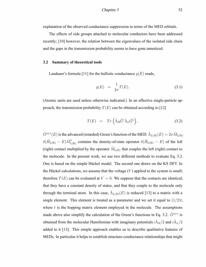
Chapitre 3 52

explanation of the observed conductance suppression in terms of the MED orbitals.

The effects of side groups attached to molecular conductors have been addressed

recently; [10] however, the relation between the eigenvalues of the isolated side chain

and the gaps in the transmission probability seems to have gone unnoticed.

3.2 Summary of theoretical tools

Landauer’s formula [11] for the ballistic conductance g(E) reads,

g(E) =1

2πT (E). (3.1)

(Atomic units are used unless otherwise indicated.) In an effective single-particle ap-

proach, the transmission probability T (E) can be obtained according to [12]

T (E) = Tr(

ΛRGrΛLG

a)

. (3.2)

Ga(r)(E) is the advanced (retarded) Green’s function of theMED. ΛL(R)(E) = 2πML(R)

δ(HL(R) − E)M †

L(R) contains the density-of-state operator δ(HL(R) − E) of the left

(right) contact multiplied by the operator ML(R) that couples the left (right) contact to

the molecule. In the present work, we use two different methods to evaluate Eq. 3.2.

One is based on the simple Hückel model. The second one draws on the KS DFT. In

the Hückel calculations, we assume that the voltage (V ) applied to the system is small;

therefore T (E) can be evaluated at V = 0. We suppose that the contacts are identical,

that they have a constant density of states, and that they couple to the molecule only

through the terminal atom. In this case, ΛL(R)(E) is reduced [13] to a matrix with a

single element. This element is treated as a parameter and we set it equal to (1/2)t,

where t is the hopping matrix element employed in the molecule. The assumptions

made above also simplify the calculation of the Green’s functions in Eq. 3.2. Ga(r) is

obtained from the molecular Hamiltonian with imaginary potentials iΛR/2 and iΛL/2

added to it [13]. This simple approach enables us to describe qualitative features of

MEDs. In particular it helps to establish structure-conductance relationships that might

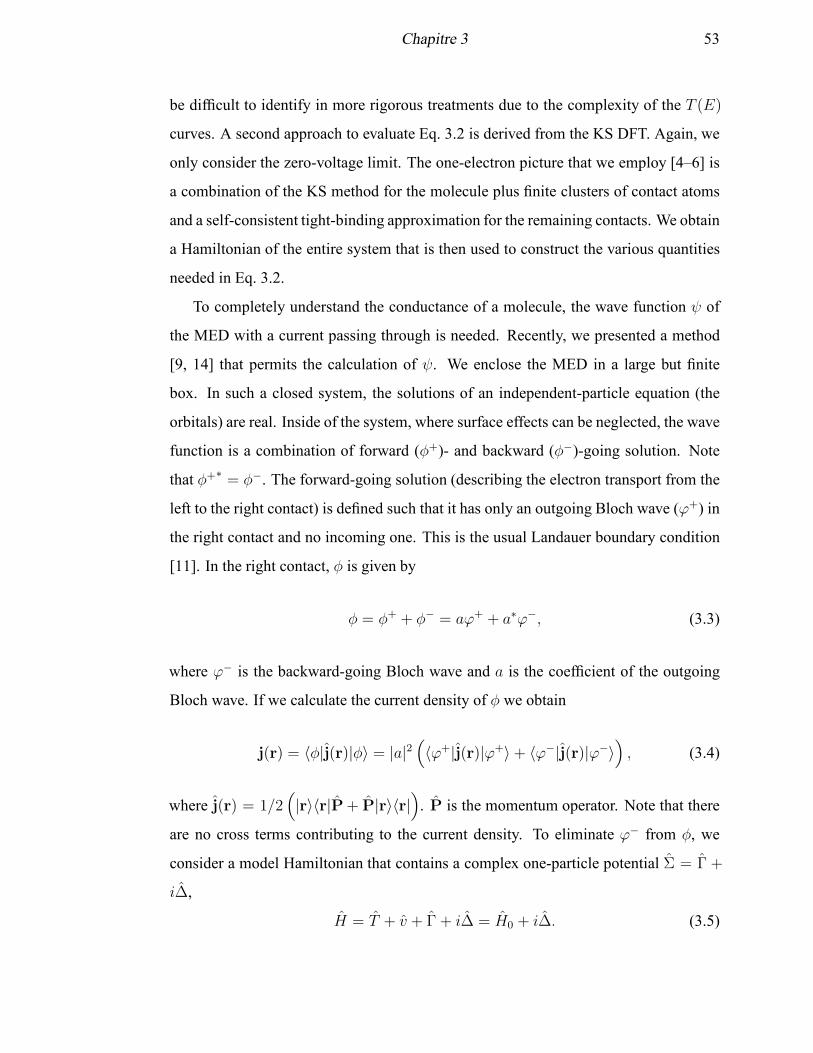
Chapitre 3 53

be difficult to identify in more rigorous treatments due to the complexity of the T (E)

curves. A second approach to evaluate Eq. 3.2 is derived from the KS DFT. Again, we

only consider the zero-voltage limit. The one-electron picture that we employ [4–6] is

a combination of the KS method for the molecule plus finite clusters of contact atoms

and a self-consistent tight-binding approximation for the remaining contacts. We obtain

a Hamiltonian of the entire system that is then used to construct the various quantities

needed in Eq. 3.2.

To completely understand the conductance of a molecule, the wave function ψ of

the MED with a current passing through is needed. Recently, we presented a method

[9, 14] that permits the calculation of ψ. We enclose the MED in a large but finite

box. In such a closed system, the solutions of an independent-particle equation (the

orbitals) are real. Inside of the system, where surface effects can be neglected, the wave

function is a combination of forward (φ+)- and backward (φ−)-going solution. Note

that φ+∗= φ−. The forward-going solution (describing the electron transport from the

left to the right contact) is defined such that it has only an outgoing Bloch wave (ϕ+) in

the right contact and no incoming one. This is the usual Landauer boundary condition

[11]. In the right contact, φ is given by

φ = φ+ + φ− = aϕ+ + a∗ϕ−, (3.3)

where ϕ− is the backward-going Bloch wave and a is the coefficient of the outgoing

Bloch wave. If we calculate the current density of φ we obtain

j(r) = 〈φ|j(r)|φ〉 = |a|2(

〈ϕ+|j(r)|ϕ+〉+ 〈ϕ−|j(r)|ϕ−〉)

, (3.4)

where j(r) = 1/2(

|r〉〈r|P+ P|r〉〈r|)

. P is the momentum operator. Note that there

are no cross terms contributing to the current density. To eliminate ϕ− from φ, we

consider a model Hamiltonian that contains a complex one-particle potential Σ = Γ +

i∆,

H = T + v + Γ + i∆ = H0 + i∆. (3.5)

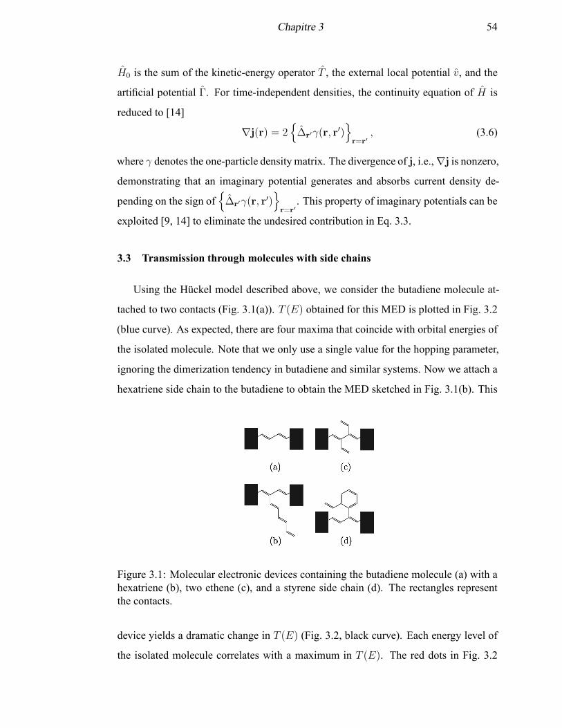
Chapitre 3 54

H0 is the sum of the kinetic-energy operator T , the external local potential v, and the

artificial potential Γ. For time-independent densities, the continuity equation of H is

reduced to [14]

∇j(r) = 2{

∆r′γ(r, r′)}

r=r′, (3.6)

where γ denotes the one-particle density matrix. The divergence of j, i.e.,∇j is nonzero,

demonstrating that an imaginary potential generates and absorbs current density de-

pending on the sign of{

∆r′γ(r, r′)}

r=r′. This property of imaginary potentials can be

exploited [9, 14] to eliminate the undesired contribution in Eq. 3.3.

3.3 Transmission through molecules with side chains

Using the Hückel model described above, we consider the butadiene molecule at-

tached to two contacts (Fig. 3.1(a)). T (E) obtained for this MED is plotted in Fig. 3.2

(blue curve). As expected, there are four maxima that coincide with orbital energies of

the isolated molecule. Note that we only use a single value for the hopping parameter,

ignoring the dimerization tendency in butadiene and similar systems. Now we attach a

hexatriene side chain to the butadiene to obtain the MED sketched in Fig. 3.1(b). This

Figure 3.1: Molecular electronic devices containing the butadiene molecule (a) with ahexatriene (b), two ethene (c), and a styrene side chain (d). The rectangles representthe contacts.

device yields a dramatic change in T (E) (Fig. 3.2, black curve). Each energy level of

the isolated molecule correlates with a maximum in T (E). The red dots in Fig. 3.2

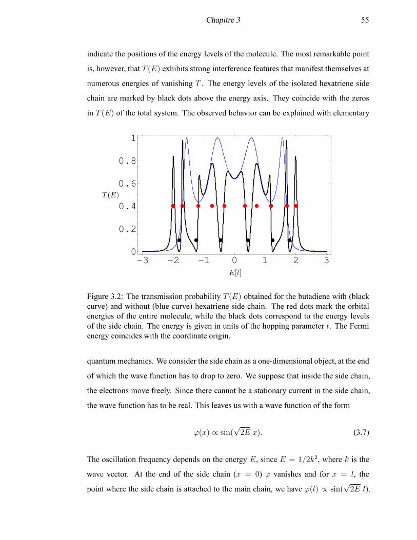
Chapitre 3 55

indicate the positions of the energy levels of the molecule. The most remarkable point

is, however, that T (E) exhibits strong interference features that manifest themselves at

numerous energies of vanishing T . The energy levels of the isolated hexatriene side

chain are marked by black dots above the energy axis. They coincide with the zeros

in T (E) of the total system. The observed behavior can be explained with elementary

-3 -2 -1 0 1 2 3

0

0.2

0.4

0.6

0.8

1

E[t]

T (E)

Figure 3.2: The transmission probability T (E) obtained for the butadiene with (blackcurve) and without (blue curve) hexatriene side chain. The red dots mark the orbitalenergies of the entire molecule, while the black dots correspond to the energy levelsof the side chain. The energy is given in units of the hopping parameter t. The Fermienergy coincides with the coordinate origin.

quantummechanics. We consider the side chain as a one-dimensional object, at the end

of which the wave function has to drop to zero. We suppose that inside the side chain,

the electrons move freely. Since there cannot be a stationary current in the side chain,

the wave function has to be real. This leaves us with a wave function of the form

ϕ(x) ∝ sin(√2E x). (3.7)

The oscillation frequency depends on the energy E, since E = 1/2k2, where k is the

wave vector. At the end of the side chain (x = 0) ϕ vanishes and for x = l, the

point where the side chain is attached to the main chain, we have ϕ(l) ∝ sin(√2E l).

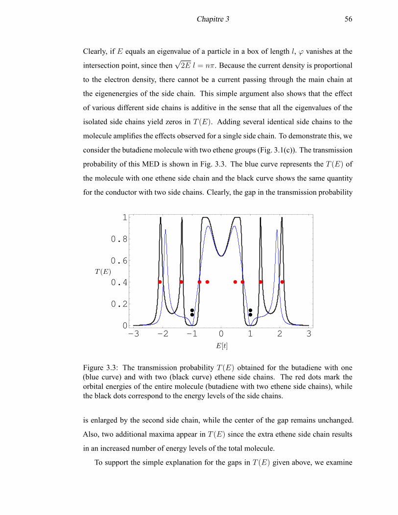
Chapitre 3 56

Clearly, if E equals an eigenvalue of a particle in a box of length l, ϕ vanishes at the

intersection point, since then√2E l = nπ. Because the current density is proportional

to the electron density, there cannot be a current passing through the main chain at

the eigenenergies of the side chain. This simple argument also shows that the effect

of various different side chains is additive in the sense that all the eigenvalues of the

isolated side chains yield zeros in T (E). Adding several identical side chains to the

molecule amplifies the effects observed for a single side chain. To demonstrate this, we

consider the butadiene molecule with two ethene groups (Fig. 3.1(c)). The transmission

probability of this MED is shown in Fig. 3.3. The blue curve represents the T (E) of

the molecule with one ethene side chain and the black curve shows the same quantity

for the conductor with two side chains. Clearly, the gap in the transmission probability

-3 -2 -1 0 1 2 3

0

0.2

0.4

0.6

0.8

1

E[t]

T (E)

Figure 3.3: The transmission probability T (E) obtained for the butadiene with one(blue curve) and with two (black curve) ethene side chains. The red dots mark theorbital energies of the entire molecule (butadiene with two ethene side chains), whilethe black dots correspond to the energy levels of the side chains.

is enlarged by the second side chain, while the center of the gap remains unchanged.

Also, two additional maxima appear in T (E) since the extra ethene side chain results

in an increased number of energy levels of the total molecule.

To support the simple explanation for the gaps in T (E) given above, we examine

Chapitre 3 57

the wave function of the di-ethene-butadiene MED. We employ the approach described

in Sec. 3.2 to generate the wave functions. The contacts are simple chains of atoms that

are coupled to each other by a hopping matrix elements of 2t. The diagonal elements

are set to zero. The chains contain 200 atoms each. The terminal five atoms of each

chain have imaginary potentials added to their diagonal matrix elements that generate

(left contact) or absorb (right contact) current density. These simple potentials are

appropriate for the energies considered here, and they are optimized to eliminate the

backward-going solution [9, 14]. The molecule is coupled to the contacts by a hopping

parameter of 0.5t and the molecular hopping parameter is set to t. t is an arbitrary

energy unit. In Fig. 3.4(a), we present the orbital at E ≈ −1, where T = 0. (Since

finite-length contacts yield discrete energy levels, we do not obtain an orbital with

exactly E = −1.) The real and the imaginary parts of this orbital are shown separately

in the upper and lower half, respectively. The imaginary part is identical to zero; thus it

is immediately obvious that this is a nonconducting orbital. Furthermore, we can indeed

verify that there are no contributions to the orbital on the atoms carrying the side chains.

An electron, emitted from the left contact enters the first side chain, gets reflected, and

returns to the contact. There is a second degenerate solution that is related to the one

depicted in Fig. 3.4(a) by inversion symmetry. This orbital is not occupied if the Fermi

energy of the left contact is sufficiently higher than the one of the right contact.

For comparison, we also display an orbital at E ≈ −0.5, where T reaches 1

(Fig. 3.4(b)). The real and the imaginary parts of this orbital are nonzero. The large

contributions to the real part that are localized on the molecule show that the molecule

is in resonance with the contacts. The coefficients on the atoms carrying a side chain

are clearly not zero.

We expect that any system that couples to a narrow molecular conductor at one

point will leave its marks in the transmission probability. Here, we do not consider

the case where there are multiple connections because this yields loops that have been

discussed elsewhere [9]. The local density of states at the attachment site of the system

connected to the molecular conductor will determine the appearance of zeros in T (E).

To illustrate this point, in Fig. 3.5, we show T (E) for the butadiene-based MED with

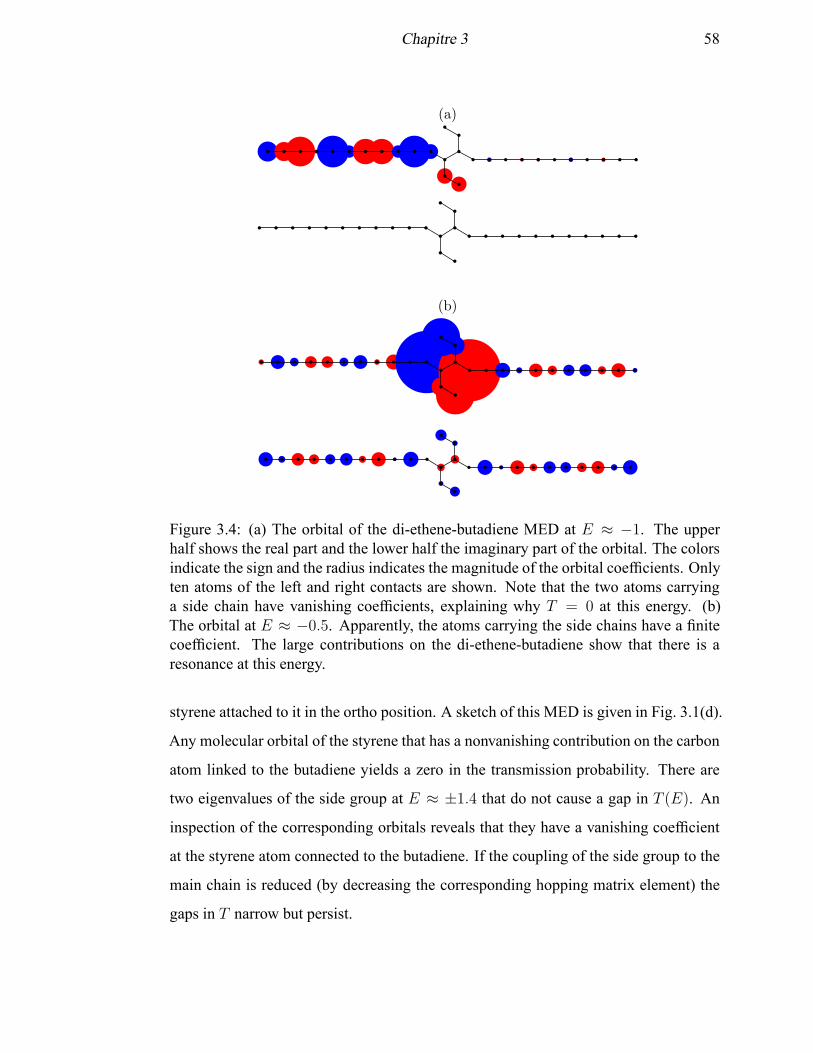
Chapitre 3 58

(a)

(b)

Figure 3.4: (a) The orbital of the di-ethene-butadiene MED at E ≈ −1. The upperhalf shows the real part and the lower half the imaginary part of the orbital. The colorsindicate the sign and the radius indicates the magnitude of the orbital coefficients. Onlyten atoms of the left and right contacts are shown. Note that the two atoms carryinga side chain have vanishing coefficients, explaining why T = 0 at this energy. (b)The orbital at E ≈ −0.5. Apparently, the atoms carrying the side chains have a finitecoefficient. The large contributions on the di-ethene-butadiene show that there is aresonance at this energy.

styrene attached to it in the ortho position. A sketch of this MED is given in Fig. 3.1(d).

Any molecular orbital of the styrene that has a nonvanishing contribution on the carbon

atom linked to the butadiene yields a zero in the transmission probability. There are

two eigenvalues of the side group at E ≈ ±1.4 that do not cause a gap in T (E). An

inspection of the corresponding orbitals reveals that they have a vanishing coefficient

at the styrene atom connected to the butadiene. If the coupling of the side group to the

main chain is reduced (by decreasing the corresponding hopping matrix element) the

gaps in T narrow but persist.

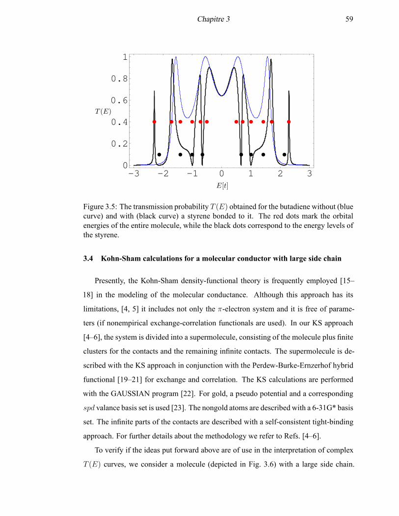
Chapitre 3 59

-3 -2 -1 0 1 2 3

0

0.2

0.4

0.6

0.8

1

E[t]

T (E)

Figure 3.5: The transmission probability T (E) obtained for the butadiene without (bluecurve) and with (black curve) a styrene bonded to it. The red dots mark the orbitalenergies of the entire molecule, while the black dots correspond to the energy levels ofthe styrene.

3.4 Kohn-Sham calculations for a molecular conductor with large side chain

Presently, the Kohn-Sham density-functional theory is frequently employed [15–

18] in the modeling of the molecular conductance. Although this approach has its

limitations, [4, 5] it includes not only the π-electron system and it is free of parame-

ters (if nonempirical exchange-correlation functionals are used). In our KS approach

[4–6], the system is divided into a supermolecule, consisting of the molecule plus finite

clusters for the contacts and the remaining infinite contacts. The supermolecule is de-

scribed with the KS approach in conjunction with the Perdew-Burke-Ernzerhof hybrid

functional [19–21] for exchange and correlation. The KS calculations are performed

with the GAUSSIAN program [22]. For gold, a pseudo potential and a corresponding

spd valance basis set is used [23]. The nongold atoms are described with a 6-31G* basis

set. The infinite parts of the contacts are described with a self-consistent tight-binding

approach. For further details about the methodology we refer to Refs. [4–6].

To verify if the ideas put forward above are of use in the interpretation of complex

T (E) curves, we consider a molecule (depicted in Fig. 3.6) with a large side chain.

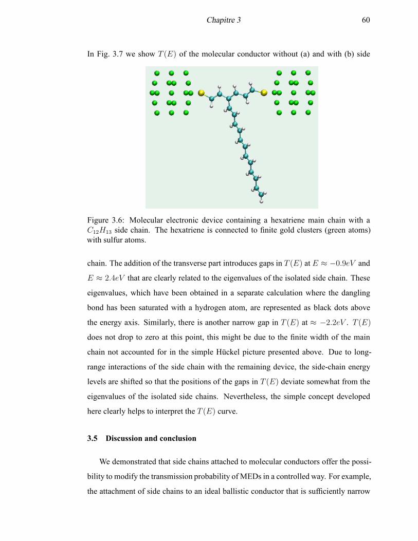
Chapitre 3 60

In Fig. 3.7 we show T (E) of the molecular conductor without (a) and with (b) side

Figure 3.6: Molecular electronic device containing a hexatriene main chain with aC12H13 side chain. The hexatriene is connected to finite gold clusters (green atoms)with sulfur atoms.

chain. The addition of the transverse part introduces gaps in T (E) at E ≈ −0.9eV and

E ≈ 2.4eV that are clearly related to the eigenvalues of the isolated side chain. These

eigenvalues, which have been obtained in a separate calculation where the dangling

bond has been saturated with a hydrogen atom, are represented as black dots above

the energy axis. Similarly, there is another narrow gap in T (E) at ≈ −2.2eV . T (E)

does not drop to zero at this point, this might be due to the finite width of the main

chain not accounted for in the simple Hückel picture presented above. Due to long-

range interactions of the side chain with the remaining device, the side-chain energy

levels are shifted so that the positions of the gaps in T (E) deviate somewhat from the

eigenvalues of the isolated side chains. Nevertheless, the simple concept developed

here clearly helps to interpret the T (E) curve.

3.5 Discussion and conclusion

We demonstrated that side chains attached to molecular conductors offer the possi-

bility to modify the transmission probability of MEDs in a controlled way. For example,

the attachment of side chains to an ideal ballistic conductor that is sufficiently narrow

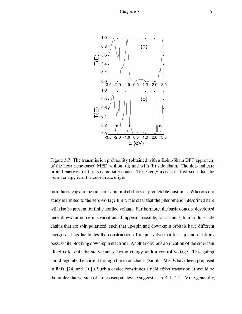
Chapitre 3 61

0.0

0.2

0.4

0.6

0.8

1.0

-3.0 -2.0 -1.0 0.0 1.0 2.0 3.0

T(E

)

E (eV)

(b)

0.0

0.2

0.4

0.6

0.8

1.0

-3.0 -2.0 -1.0 0.0 1.0 2.0 3.0

T(E

)

(a)

Figure 3.7: The transmission probability (obtained with a Kohn-Sham DFT approach)of the hexatriene-based MED without (a) and with (b) side chain. The dots indicateorbital energies of the isolated side chain. The energy axis is shifted such that theFermi energy is at the coordinate origin.

introduces gaps in the transmission probabilities at predictable positions. Whereas our

study is limited to the zero-voltage limit, it is clear that the phenomenon described here

will also be present for finite applied voltage. Furthermore, the basic concept developed

here allows for numerous variations. It appears possible, for instance, to introduce side

chains that are spin polarized, such that up-spin and down-spin orbitals have different

energies. This facilitates the construction of a spin valve that lets up-spin electrons

pass, while blocking down-spin electrons. Another obvious application of the side-cain

effect is to shift the side-chain states in energy with a control voltage. This gating

could regulate the current through the main chain. (Similar MEDs have been proposed

in Refs. [24] and [10].) Such a device constitutes a field effect transistor. It would be

the molecular version of a mesoscopic device suggested in Ref. [25]. More generally,

Chapitre 3 62

MEDs with delocalized π-electron systems can be regarded as a molecular version of

quantum waveguides (Ref. [26] and references therein).

Acknowledgements

We would like to acknowledge the financial support provided by NSERC through

grant 238404-03.

Chapitre 3 63

3.6 Bibliography

[1] Molecular Electronics: Science and Technology, edited by A. Aviram and M. Rat-

ner (New York Academy of Sciences, New York, 1998).

[2] A. Nitzan, Annu. Rev. Phys. Chem. 52, 681 (2001).

[3] A. Nitzan and M. A. Ratner, Science 300, 1384 (2003).

[4] M. Ernzerhof and M. Zhuang, Int. J. Quantum Chem. 101, 557 (2005).

[5] M. Zhuang, P. Rocheleau, and M. Ernzerhof, J. Chem. Phys. 122, 154705 (2005).

[6] M. Zhuang and M. Ernzerhof, Phys. Rev. B 72, 073104 (2005).

[7] P. Sautet and C. Joachim, Chem. Phys. Lett. 153, 511 (1988).

[8] D. Walter, D. Neuhauser, and R. Baer, Chem. Phys. 299, 139 (2004).

[9] M. Ernzerhof, H. Bahmann, M. Zhuang, and P. Rocheleau, J. Chem. Phys. (sub-

mitted).

[10] R. Collepardo-Guevara, D. Walter, D. Neuhauser, and R. Baer, Chem. Phys. Lett.

393, 367 (2004).

[11] R. Landauer, Philos. Mag. 21, 863 (1970).

[12] Y. Meir and N. S. Wingreen, Phys. Rev. Lett. 68, 2512 (1992).

[13] L. E. Hall, J. R. Reimers, N. S. Hush, and K. Silverbrook, J. Chem. Phys. 112,

1510 (2000).

[14] M. Ernzerhof and M. Zhuang, J. Chem. Phys. 119, 4134 (2003).

[15] J. Taylor, H. Guo, and J. Wang, Phys. Rev. B 63, 245407 (2001).

[16] P. S. Damle, A. W. Ghosh, and S. Datta, Phys. Rev. B 64, 201403 (2001).

[17] M. Brandbyge, J.-L. Mozos, P. Ordejón, J. Taylor, and K. Stokbro, Phys. Rev. B

65, 165401 (2002).

Chapitre 3 64

[18] Y. Xue, S. Datta, and M. A. Ratner, J. Chem. Phys. 115, 4292 (2001).

[19] J. P. Perdew, M. Ernzerhof, and K. Burke, J. Chem. Phys. 105, 9982 (1996).

[20] M. Ernzerhof and G. E. Scuseria, J. Chem. Phys. 110, 5029 (1999).

[21] M. Ernzerhof, J. P. Perdew, and K. Burke, Int. J. Quantum Chem. 64, 285 (1997).



[23] R. B. Ross, J. M. Powers, T. Atashroo, W. C. Ermler, L. A. LaJohn, and P. A.

Christiansen, J. Chem. Phys. 93, 6654 (1990).

[24] R. Baer and D. Neuhauser, Chem. Phys. 281, 353 (2002).

[25] F. Sols, M. Macucci, U. Ravaioli, and K. Hess, Appl. Phys. Lett. 54, 350 (1989).

[26] P. S. Deo and A. M. Jayannavar, Phys. Rev. B 50, 11629 (1994).

CHAPITRE 4

ELECTRON TRANSMISSION THROUGH

AROMATIC MOLECULES

Matthias Ernzerhof, Hilke Bahmann, Francois Goyer, Min Zhuang, and Philippe

Rocheleau



Reproduit avec la permission de Matthias Ernzerhof, Hilke Bahmann, Francois Goyer,

Min Zhuang, and Philippe Rocheleau Journal of Chemical Theory and Computation,

Vol. 2, 1291-1297, (2006). Copyright 2006, American Chemical Society.

Chapitre 4 66


Cet article porte sur la transmission électronique des molécules aromatiques en uti-

lisant par exemple, les molécules de benzène et de coronène. Les caractéristiques de

transport de ces molécules sont analysées à l’aide de la distribution du courant à l’in-

térieur des molécules. Nous notons la présence de courants circulaires importants et

émettons l’hypothèse que le champ magnétique généré par ces courants pourrait être

mesurable expérimentalement. Hilke Bahmann et Francois Goyer ont principalement

développé la méthode pour calculer et analyser la distribution du courant. Min Zhuang

a élaboré l’article et créé des exemples inclus dans l’article alors que Philippe Roche-

leau a élaboré l’article, créé des exemples et rédigé la section concernant le champ

magnétique généré par les courants circulaires. Matthias Ernzerhof a supervisé les tra-

vaux, contribué à l’interprétation des résultats et à la révision du manuscrit.

Chapitre 4 67

ABSTRACT

A prominent feature of aromatic compounds is the ring current that can be observed

indirectly in nuclear magnetic resonance experiments. This current is generated by an

external magnetic field. In molecular electronics, molecules serve as conductors, and

they are connected to metallic contacts that act as electron sources and electron sinks.

We show that ring currents can also be found in molecular electronic devices containing

cyclic π-electron systems. The circular currents are related to interference phenomena

that can render the molecule impenetrable to electrons. While only small currents pass

through the molecule, large internal circular currents are stimulated. We conjecture that

the internal currents should result in experimentally observable magnetic moments.

Chapitre 4 68

4.1 Introduction

To consider molecules as conductors [1–4] is a subject that has recently attracted much

attention. Our understanding of electron transport through molecules is presently far

from complete, and the mechanisms underlying molecular conductance are only now

beginning to be explored. In this context theoretical studies of molecular conductors

are a valuable tool that even allow us to conceive new experiments and predict their

outcome. In fact, molecular electronic devices (MEDs) have first been suggested in a

theoretical article [5]. It should, however, be noted that MEDs represent an enormous

theoretical challenge and that our methods of modelling MEDs [6–13] are still in their

infancy. In particular correlation effects are difficult to account for properly [14].

An interesting question that arises in molecular electronics is whether established

concepts of chemistry are still useful in the analysis of MEDs. Here, we consider the

notion of the ring current that is a prominent feature of aromatic systems. Employing

the simple Hückel model, we investigate the conductance of benzene and coronene,

and we find indeed that ring currents are crucial to rationalize the transmission of elec-

trons through aromatic molecules. We demonstrate that benzene and coronene exhibit

prominent negative interference effects that are related to ring currents. Investigations

similar to ours have already been performed for related systems [15]. In Ref. [16] the

electron transmission probability for the benzene molecule with wires attached to it is

discussed. An analysis of the molecular orbitals is presented to explain the interference

phenomena observed. Maybe the most important advance made here, in comparison to

earlier work, is that we analyze the internal current distribution in the molecule. We be-

lieve that this distribution is essential to fully understand the current transport through

MEDs. From the molecular current distribution, we are able to calculate the magnetic

moment generated by the ring currents. We predict that coronene, with a voltage ap-

plied to it, could generate a magnetic moment of several µB, where µB = (e~)/(2me)

is Bohr’s magneton. The determining feature of the molecular conductors examined

here is their circular delocalized π-electron system. This type of system continues to

attract attention. Recently, the behavior of circular molecular conductors in magnetic

Chapitre 4 69

fields has been studied (for review see ref [17]). Three-terminal circular logic gates

have been proposed [18] and the dependence of the transmittance on the arrangement

of the leads attached to a circular conductor has been investigated [19].

In the remainder of this paper we use atomic units (me = e2 = ~ = 1), unless

indicated otherwise.

4.2 Summary of theoretical concepts

A basic tool of molecular electronics is Landauer’s formula [20] for the ballistic con-

ductance g(E),

g(E) =1

2πT (E) (4.1)

(Note that the conductance quantum (e2/h) reduces to (1/2π) in atomic units.) If

electron-electron interaction is considered through an effective single-particle approach,

the transmission probability T (E) can be obtained according to [6–8]

T (E) = Tr (ΓRGrΓLG

a) (4.2)

where Ga(r)(E) is the advanced (retarded) Green’s function of the entire system.

ΓL(R)(E) = 2πML(R)δ(HL(R)−E)M†

L(R) contains the density of state operator δ(HL(R)−E) of the left (right) contact multiplied by the operator ML(R) that couples the left

(right) contact to the molecule. Numerous strategies are available to implement (see

e.g., refs [10–12] and [21–23]) this formula. Here we are interested in the properties of

delocalized π systems, and it is known that the qualitative features of such systems can

be reproduced with a simple Hückel model. Furthermore, we assume that the voltage

applied to the system is small, such that its polarizing effect on the orbitals and thus on

T (E) can be neglected. Finally, we suppose that the contacts are identical, that they

have a constant density of states (this is sometimes called the wide band limit), and

that they couple to the molecule only through the molecular atom that is attached to

the chain. In this case, ΓL(R)(E) reduces [24] to a matrix with a single element. This

Chapitre 4 70

element is treated as a parameter in our work, and we set it equal to the hopping matrix

element used in the molecule. By varying the coupling strength, we ensured that the

qualitative conclusions drawn here are not sensitive to the exact value of this parameter.

We stress that in the present work we do not attempt to describe quantitative but rather

qualitative effects that are robust with respect to the choice of the model parameters

and with respect to the choice of the theoretical method employed to calculate T (E).

The simple approach just described makes it possible to quickly examine T (E) of nu-

merous structures. All the T versus E curves presented here have been generated with

this scheme, the exception being Figure 4.9 described in the Appendix.

One of the main aims of our work is to use the internal current distribution as a

tool to understand molecular conductance. All the current distributions presented in

the following have been obtained with a method that we developed recently and that

will be described in detail in a forthcoming publication [25]. Here we provide a short

outline. We consider a finite model of a MED, the Hamiltonian of which contains a

complex one-particle potential Σ

H = T + v + Σ (4.3)

The Hamiltonian operator in eq 4.3 is non-Hermitian, nevertheless it permits the de-

velopment of a consistent quantum mechanics [25]. To show that the Hamiltonian in

eq 4.3 enables us to describe an MED with a stationary current passing through, we

consider a one-dimensional contact along the x axis that extends from −∞ to 0. This

contact represents the left contact of a MED, and, at x = 0, we attach the molecule it.

In the left contact, sufficiently far away from the molecule, the wave function ϕ is a

combination of a forward going Bloch wave ϕ+(x) and a backward going Bloch wave

ϕ−(x)

ϕ(x)left contact

= aϕ+(x) + bϕ−(x) (4.4)

Since we want our model system to be finite, we multiply ϕ(x) by a damping factor

fL(x). This function takes a value of one in the region that includes the molecule and

Chapitre 4 71

beyond (x→ ∞), and it drops to zero inside of the left contact. We define

φ(x)left contact

= fL(x)ϕ(x) (4.5)

The damping factor fL(x) is of course not unique, but this does not pose a problem for

our approach. Inserting φ into the stationary Schrödinger equation

(

−1

2∆ + v + Σ

)

φleft contact

= Eφ (4.6)

and subsequent inversion of this equation yields an expression for the potential Σ = ΣL + ΣR

in the left contact

ΣL(x)left contact

=∆φ(x)

2φ(x)− v(x) + E (4.7)

Multiplication of φ by a constant does not change the value of the potential ΣL. This

allows us to eliminate the coefficient a in eq 4.4, and we are left with one unknown

complex parameter r = b/a in ΣL. Note that for |r| = 1 there is no net current flow

since forward and backward going Bloch wave have the same weight. In this case ΣL

is a real potential. If the molecule is transparent (T = 1), then r = 0. For |r| 6= 1, ΣL

is complex.

In the right contact that starts at x = l, we only have a forward going Bloch wave

(ϕ+) that we damp by a function fR(x) that drops to zero at some distance from the

molecule. Similar to fL(x), fR(x) is equal to one in the physical region including the

molecule and beyond (x→ −∞). We have

φ(x)right contact

= cfR(x)ϕ+(x) (4.8)

Inversion of the Schrödinger equation with the wave function in eq 4.8 yields ΣR. The

parameter c cancels out of the equation for ΣR.

Equation 4.7 allows us to calculate ΣL as a function of the parameter r that in turn

depends on the energy E. r is directly related to T (E) by

T (E) = 1− |r(E)|2 (4.9)

Chapitre 4 72

The remaining question is then how to obtain r? The condition that an eigenvalue

of the model Hamiltonian in eq 4.3 is identical to the energy chosen in the potential

ΣL(R) suffices [13, 25] to determine r. Note that the energy (and the eigenvalue of H)

of interest is real. The ideas just described are readily applied to the Hückel model

[25]. The contacts, represented by infinite chains of equidistant atoms, are replaced by

complex potentials. From the wave function that we obtain, we calculate the current

distribution (using eq 4.10, given below). We verified that our model Hamiltonian

yields the exact T (E) of the underlying infinite system in which the contacts have not

been replaced by Σ.

As mentioned above, the T (E) curves presented are obtained from eq 4.2 in the

wide band limit. The features discussed here do not depend on which method we use,

however. To demonstrate this, in the Appendix, T (E) obtained from our non-Hermitian

model Hamiltonian is compared to T (E) obtained from eq 4.2.

In the Hückel model, that we employ in the present work, there are no continuous

spatial variables. Instead, all equations are formulated in a finite-dimensional vector

space. While the formulas given above can be transferred in a straightforward fashion

to the Hückel model, it is useful to provide the expression for the current density. We

find that the current density along a bond joining atom k and l is

jk→l = i(c∗ktcl − c∗l tck) (4.10)

where the hopping matrix element between the atoms is t, and ck is an orbital coeffi-

cient. Between two bound atoms, the Hückel model is effectively a one-dimensional

model, and, in one dimension, the current density and the current are identical. The di-

vergence of the current (∇j) in the Hückel model is simply the difference between the

current flowing in to and out of an atom. Apparently,∇j should be zero unless the atom

in question has an imaginary matrix element. Finally, we list the Hückel parameters em-

ployed in the calculations. The on-site energies are set to zero. The hopping parameter

in the contact chains is 1.4t, where t is the hopping parameter in the molecule. The

coupling matrix element between the contact and the molecule is also t.

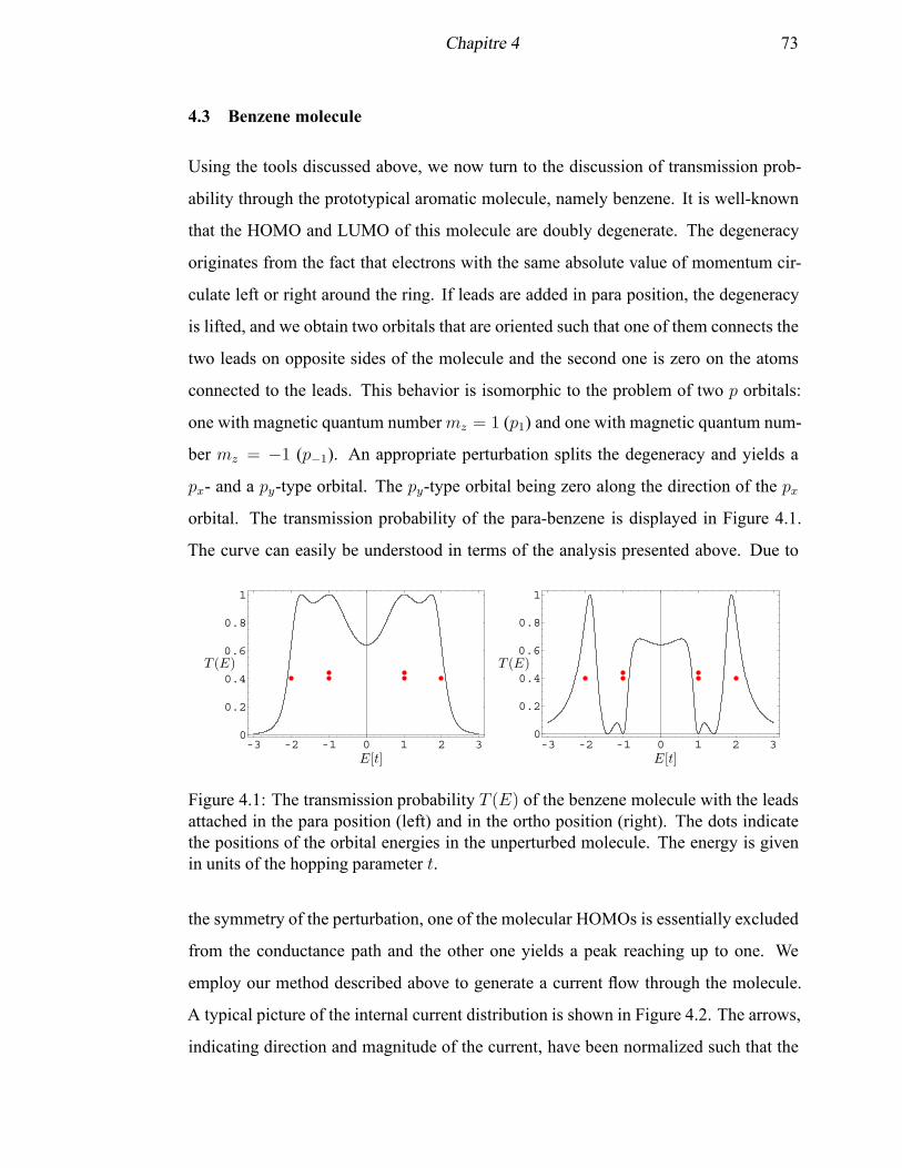
Chapitre 4 73

4.3 Benzene molecule

Using the tools discussed above, we now turn to the discussion of transmission prob-

ability through the prototypical aromatic molecule, namely benzene. It is well-known

that the HOMO and LUMO of this molecule are doubly degenerate. The degeneracy

originates from the fact that electrons with the same absolute value of momentum cir-

culate left or right around the ring. If leads are added in para position, the degeneracy

is lifted, and we obtain two orbitals that are oriented such that one of them connects the

two leads on opposite sides of the molecule and the second one is zero on the atoms

connected to the leads. This behavior is isomorphic to the problem of two p orbitals:

one with magnetic quantum numbermz = 1 (p1) and one with magnetic quantum num-

ber mz = −1 (p−1). An appropriate perturbation splits the degeneracy and yields a

px- and a py-type orbital. The py-type orbital being zero along the direction of the px

orbital. The transmission probability of the para-benzene is displayed in Figure 4.1.

The curve can easily be understood in terms of the analysis presented above. Due to

-3 -2 -1 0 1 2 30

0.2

0.4

0.6

0.8

1

E[t]

T (E)

-3 -2 -1 0 1 2 30

0.2

0.4

0.6

0.8

1

E[t]

T (E)

Figure 4.1: The transmission probability T (E) of the benzene molecule with the leadsattached in the para position (left) and in the ortho position (right). The dots indicatethe positions of the orbital energies in the unperturbed molecule. The energy is givenin units of the hopping parameter t.

the symmetry of the perturbation, one of the molecular HOMOs is essentially excluded

from the conductance path and the other one yields a peak reaching up to one. We

employ our method described above to generate a current flow through the molecule.

A typical picture of the internal current distribution is shown in Figure 4.2. The arrows,

indicating direction and magnitude of the current, have been normalized such that the

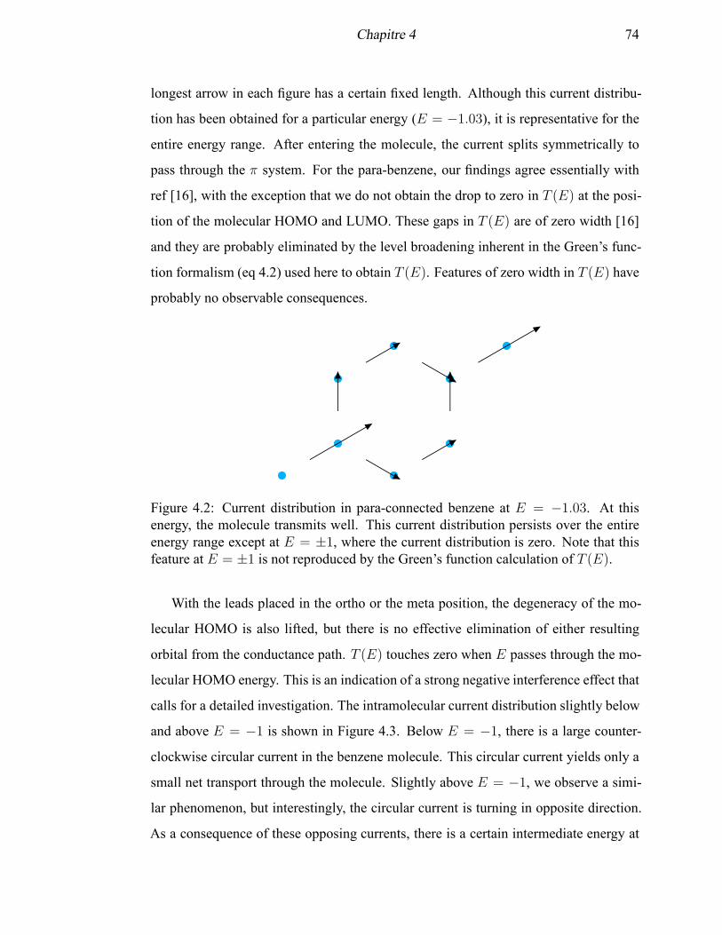
Chapitre 4 74

longest arrow in each figure has a certain fixed length. Although this current distribu-

tion has been obtained for a particular energy (E = −1.03), it is representative for the

entire energy range. After entering the molecule, the current splits symmetrically to

pass through the π system. For the para-benzene, our findings agree essentially with

ref [16], with the exception that we do not obtain the drop to zero in T (E) at the posi-

tion of the molecular HOMO and LUMO. These gaps in T (E) are of zero width [16]

and they are probably eliminated by the level broadening inherent in the Green’s func-

tion formalism (eq 4.2) used here to obtain T (E). Features of zero width in T (E) have

probably no observable consequences.

Figure 4.2: Current distribution in para-connected benzene at E = −1.03. At thisenergy, the molecule transmits well. This current distribution persists over the entireenergy range except at E = ±1, where the current distribution is zero. Note that thisfeature at E = ±1 is not reproduced by the Green’s function calculation of T (E).

With the leads placed in the ortho or the meta position, the degeneracy of the mo-

lecular HOMO is also lifted, but there is no effective elimination of either resulting

orbital from the conductance path. T (E) touches zero when E passes through the mo-

lecular HOMO energy. This is an indication of a strong negative interference effect that

calls for a detailed investigation. The intramolecular current distribution slightly below

and above E = −1 is shown in Figure 4.3. Below E = −1, there is a large counter-

clockwise circular current in the benzene molecule. This circular current yields only a

small net transport through the molecule. Slightly above E = −1, we observe a simi-

lar phenomenon, but interestingly, the circular current is turning in opposite direction.

As a consequence of these opposing currents, there is a certain intermediate energy at

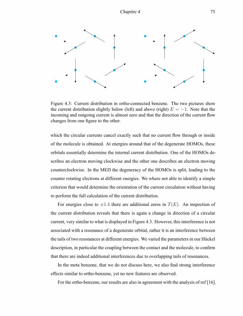
Chapitre 4 75

Figure 4.3: Current distribution in ortho-connected benzene. The two pictures showthe current distribution slightly below (left) and above (right) E = −1. Note that theincoming and outgoing current is almost zero and that the direction of the current flowchanges from one figure to the other.

which the circular currents cancel exactly such that no current flow through or inside

of the molecule is obtained. At energies around that of the degenerate HOMOs, these

orbitals essentially determine the internal current distribution. One of the HOMOs de-

scribes an electron moving clockwise and the other one describes an electron moving

counterclockwise. In the MED the degeneracy of the HOMOs is split, leading to the

counter rotating electrons at different energies. We where not able to identify a simple

criterion that would determine the orientation of the current circulation without having

to perform the full calculation of the current distribution.

For energies close to ±1.4 there are additional zeros in T (E). An inspection of

the current distribution reveals that there is again a change in direction of a circular

current, very similar to what is displayed in Figure 4.3. However, this interference is not

associated with a resonance of a degenerate orbital, rather it is an interference between

the tails of two resonances at different energies. We varied the parameters in our Hückel

description, in particular the coupling between the contact and the molecule, to confirm

that there are indeed additional interferences due to overlapping tails of resonances.

In the meta benzene, that we do not discuss here, we also find strong interference

effects similar to ortho-benzene, yet no new features are observed.

For the ortho-benzene, our results are also in agreement with the analysis of ref [16].

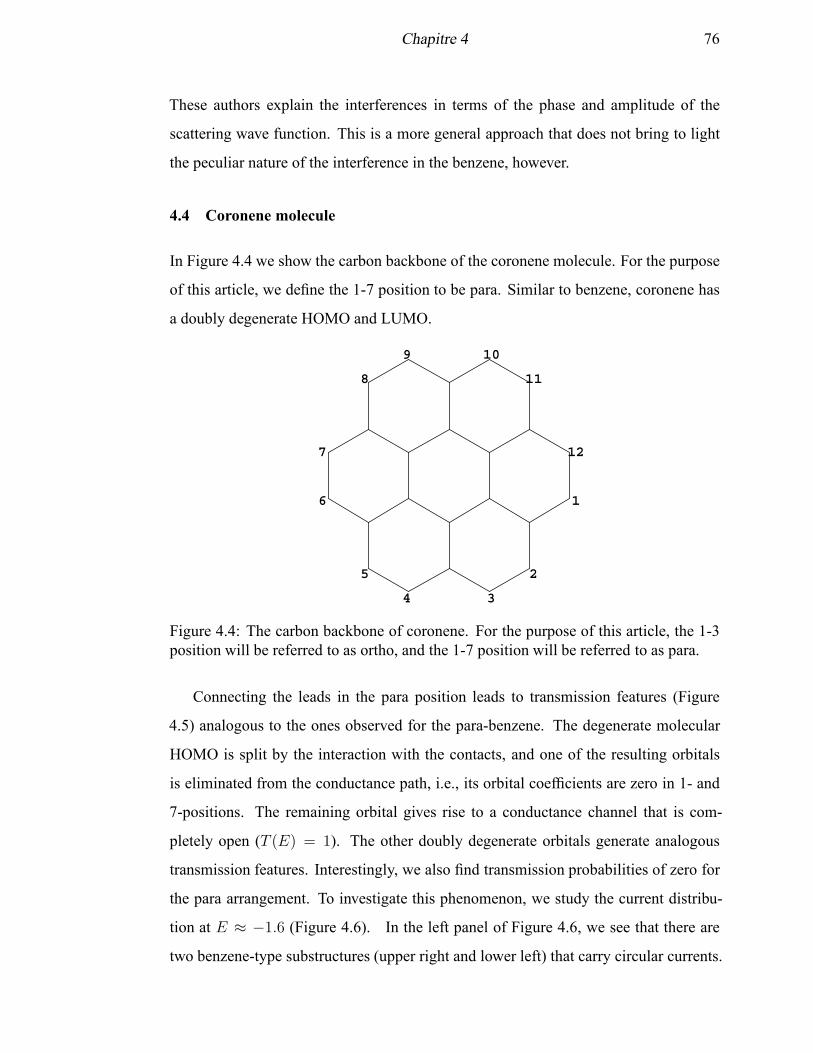
Chapitre 4 76

These authors explain the interferences in terms of the phase and amplitude of the

scattering wave function. This is a more general approach that does not bring to light

the peculiar nature of the interference in the benzene, however.

4.4 Coronene molecule

In Figure 4.4 we show the carbon backbone of the coronene molecule. For the purpose

of this article, we define the 1-7 position to be para. Similar to benzene, coronene has

a doubly degenerate HOMO and LUMO.

1

2

34

5

6

7

8

9 10

11

12

Figure 4.4: The carbon backbone of coronene. For the purpose of this article, the 1-3position will be referred to as ortho, and the 1-7 position will be referred to as para.

Connecting the leads in the para position leads to transmission features (Figure

4.5) analogous to the ones observed for the para-benzene. The degenerate molecular

HOMO is split by the interaction with the contacts, and one of the resulting orbitals

is eliminated from the conductance path, i.e., its orbital coefficients are zero in 1- and

7-positions. The remaining orbital gives rise to a conductance channel that is com-

pletely open (T (E) = 1). The other doubly degenerate orbitals generate analogous

transmission features. Interestingly, we also find transmission probabilities of zero for

the para arrangement. To investigate this phenomenon, we study the current distribu-

tion at E ≈ −1.6 (Figure 4.6). In the left panel of Figure 4.6, we see that there are

two benzene-type substructures (upper right and lower left) that carry circular currents.

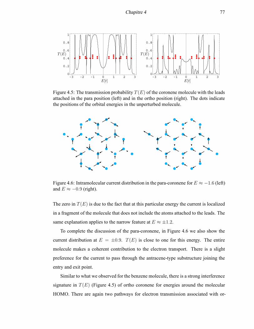
Chapitre 4 77

-3 -2 -1 0 1 2 30

0.2

0.4

0.6

0.8

1

E[t]

T (E)

-3 -2 -1 0 1 2 30

0.2

0.4

0.6

0.8

1

E[t]

T (E)

Figure 4.5: The transmission probability T (E) of the coronene molecule with the leadsattached in the para position (left) and in the ortho position (right). The dots indicatethe positions of the orbital energies in the unperturbed molecule.

Figure 4.6: Intramolecular current distribution in the para-coronene forE ≈ −1.6 (left)and E ≈ −0.9 (right).

The zero in T (E) is due to the fact that at this particular energy the current is localized

in a fragment of the molecule that does not include the atoms attached to the leads. The

same explanation applies to the narrow feature at E ≈ ±1.2.

To complete the discussion of the para-coronene, in Figure 4.6 we also show the

current distribution at E = ±0.9. T (E) is close to one for this energy. The entire

molecule makes a coherent contribution to the electron transport. There is a slight

preference for the current to pass through the antracene-type substructure joining the

entry and exit point.

Similar to what we observed for the benzene molecule, there is a strong interference

signature in T (E) (Figure 4.5) of ortho coronene for energies around the molecular

HOMO. There are again two pathways for electron transmission associated with or-

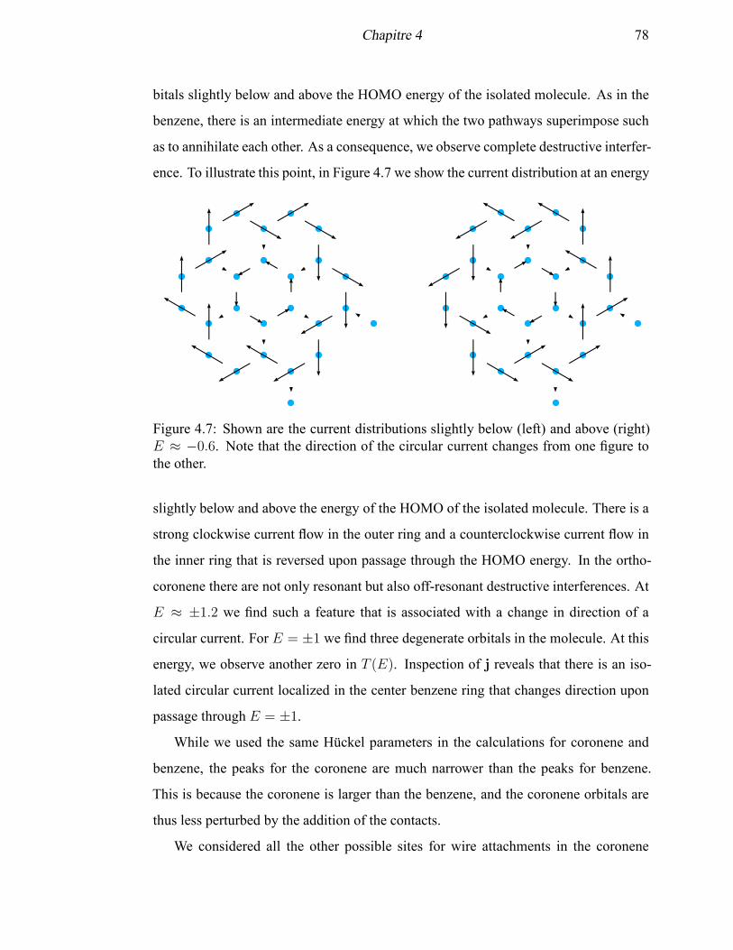
Chapitre 4 78

bitals slightly below and above the HOMO energy of the isolated molecule. As in the

benzene, there is an intermediate energy at which the two pathways superimpose such

as to annihilate each other. As a consequence, we observe complete destructive interfer-

ence. To illustrate this point, in Figure 4.7 we show the current distribution at an energy

Figure 4.7: Shown are the current distributions slightly below (left) and above (right)E ≈ −0.6. Note that the direction of the circular current changes from one figure tothe other.

slightly below and above the energy of the HOMO of the isolated molecule. There is a

strong clockwise current flow in the outer ring and a counterclockwise current flow in

the inner ring that is reversed upon passage through the HOMO energy. In the ortho-

coronene there are not only resonant but also off-resonant destructive interferences. At

E ≈ ±1.2 we find such a feature that is associated with a change in direction of a

circular current. For E = ±1 we find three degenerate orbitals in the molecule. At this

energy, we observe another zero in T (E). Inspection of j reveals that there is an iso-

lated circular current localized in the center benzene ring that changes direction upon

passage through E = ±1.

While we used the same Hückel parameters in the calculations for coronene and

benzene, the peaks for the coronene are much narrower than the peaks for benzene.

This is because the coronene is larger than the benzene, and the coronene orbitals are

thus less perturbed by the addition of the contacts.

We considered all the other possible sites for wire attachments in the coronene

Chapitre 4 79

molecule. In all cases we find similar interference patterns as the ones described here.

4.5 Observable consequences of the predicted circular currents

In the previous sections we showed that the concept of a ring current plays an important

role in the interpretation of the transmission probabilities. We saw that large circular

currents may be induced by the external contacts even if little current is flowing through

the molecule. These circular currents should generate a magnetic moment m, normal

to the molecular plane, that might be observable. To further elaborate on this issue, we

calculatem as a function of the energy for the coronene. We are only interested in the

contribution from the molecule, and we neglect contributions tom due to the contacts.

The magnetic moment of a wire in a plane with current I passing through is [26]

m =1

2

∫

r× dI (4.11)

where dI is a vector that points in the direction of the wire. The length of dI is scaled

by I . Evaluation of this formula within the Hückel model yields [27]

m(E) =1

2

∑

i>k

jik(E)(ri × rk) (4.12)

jik(E) is the current flowing along the bond (ik) in an orbital with energy E. ri and

rj are the positions of atom i and j, respectively. Since coronene is planar, m(E) is

perpendicular to the molecular plane, parallel to the z-axis. A plot ofmz(E) is shown in

Figure 4.8. In agreement with the observation of circular currents of rapidly changing

orientation, there are strong variations in mz(E). For negative energies, we observe

three large oscillations. These oscillations are generated by electrons circulating in

the molecule in opposing directions, depending on their energy. Note that the large

circular currents, i.e., large magnetic moments are associated with doubly degenerate

molecular orbitals. As mentioned earlier, the 3-fold degenerate molecular level yields

a circular current in a benzene-type substructure. Correspondingly, we observe a small

oscillation in mz at E = ±1. We should point out that the calculation of mz is only

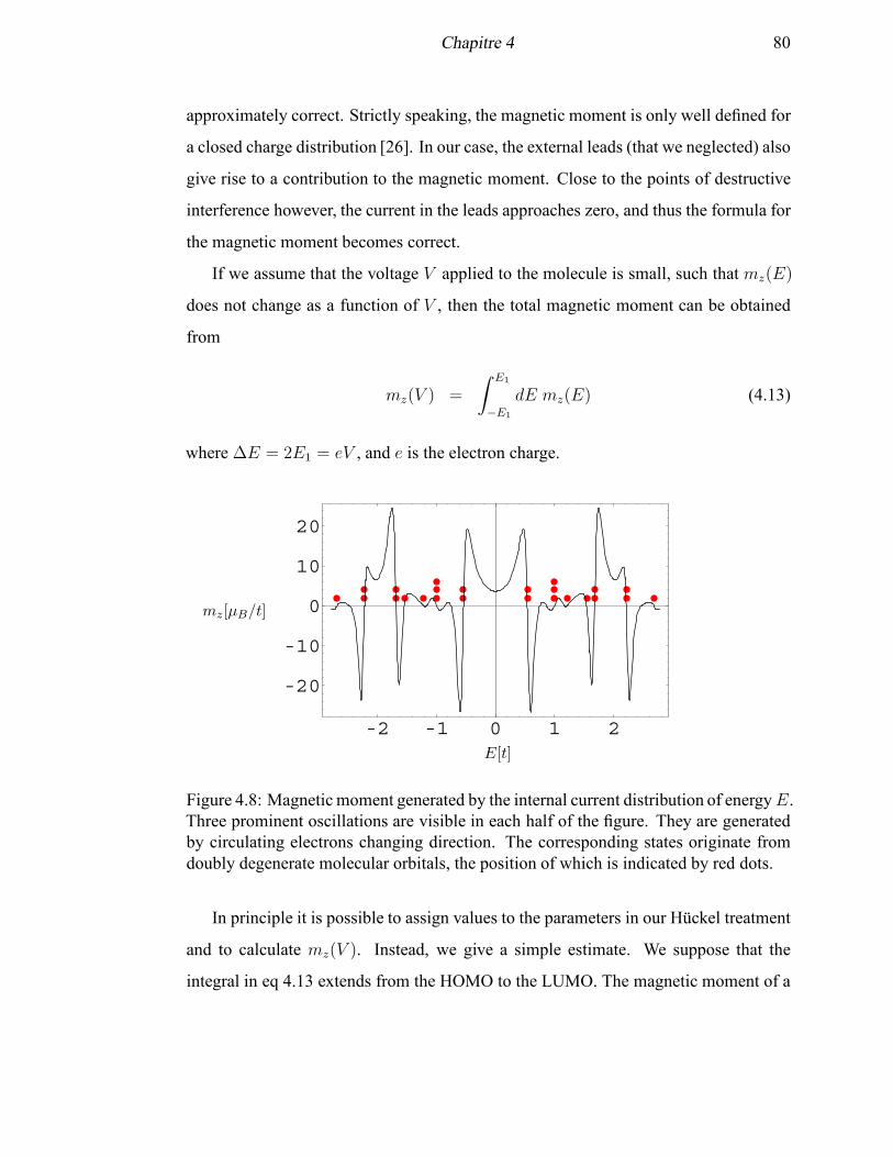
Chapitre 4 80

approximately correct. Strictly speaking, the magnetic moment is only well defined for

a closed charge distribution [26]. In our case, the external leads (that we neglected) also

give rise to a contribution to the magnetic moment. Close to the points of destructive

interference however, the current in the leads approaches zero, and thus the formula for

the magnetic moment becomes correct.

If we assume that the voltage V applied to the molecule is small, such that mz(E)

does not change as a function of V , then the total magnetic moment can be obtained

from

mz(V ) =

∫ E1

−E1

dE mz(E) (4.13)

where ∆E = 2E1 = eV , and e is the electron charge.

-2 -1 0 1 2

-20

-10

0

10

20

E[t]

mz[µB/t]

Figure 4.8: Magnetic moment generated by the internal current distribution of energyE.Three prominent oscillations are visible in each half of the figure. They are generatedby circulating electrons changing direction. The corresponding states originate fromdoubly degenerate molecular orbitals, the position of which is indicated by red dots.

In principle it is possible to assign values to the parameters in our Hückel treatment

and to calculate mz(V ). Instead, we give a simple estimate. We suppose that the

integral in eq 4.13 extends from the HOMO to the LUMO. The magnetic moment of a

Chapitre 4 81

circular current is given by

µ = I A (4.14)

where I is the current, and A the surface area encircled by the current. The current can

be obtained by

I =eh

2πmrλ(4.15)

where e is the electron charge, m the electron mass, r is the radius of the circle de-

scribed by the current I, and λ the electron wavelength. λ can be determined by inspec-

tion of the coronene π-electron system. The HOMO of coronene has an alternating

bonding and antibonding structure. With this in mind, the electron wavelength in the

HOMO is estimated to be four bond lengths (5.6 Å). By using eqs 4.14 and 4.15, we

obtain a magnetic moment of about 4.1µB for an electron circling on the outer ring of

coronene. Because of spin degeneracy, this value has to be multiplied by a factor of

2. Furthermore, to estimate mz(V ) in eq 4.13, where the moment is generated by the

HOMO and the LUMO, we multiply by an additional factor of 2. Altogether, we obtain

mz ≈ 16.4µB. This is a magnetic moment that might be observable experimentally.

4.6 Discussion and conclusion

For the representative aromatic molecules considered, we find that the most striking

features in T (E) are caused by negative interferences. By analyzing the internal cur-

rent distribution, we demonstrate that often the interferences are related to opposing

ring currents. Other interferences lead to localization of the current distribution in a

substructure of the molecule that excludes atoms connected to the contacts.

One of the few studies of intramolecular current distributions has been performed

for the C60 molecule [27]. Circular currents have also been observed in this system.

In ref [27] and in our own studies on C60, it was found that for energies around the

HOMO/LUMO there are no "global" current circulations, rather vortices are observed

Chapitre 4 82

in five-membered rings. We conclude that the magnetic moments generated in C60

are much weaker than the ones reported here. (The moment is proportional to the area

enclosed by the current).

There is presently a renewed interest [28] in large circular π-electron systems be-

cause of their potential to exhibit the Aharonov-Bohm effect [29]. The giant circular

molecule with ≈ 12nm in diameter recently synthesized [28], and systems such as

Kekulene [30] might produce enormous magnetic moments in molecular conductance

experiments. Although only small currents will pass through the molecule at the appro-

priate insertion energy, we predict that there will be large intramolecular currents. Until

now, it appears that only para connected aromatic molecules have been investigated ex-

perimentally. The large molecules mentioned might permit a nonpara connection to the

contacts that is difficult to realize with benzene and other small systems.

In the present work, we neglected the polarizing effect that an applied external field

would have on the electronic structure. A finite applied voltage might considerably dis-

tort the molecular orbitals and hinder the appearance of circular currents. Furthermore,

variations in the number of π-electrons (due to the contacts) can introduce geometry

changes that also reduce the π-electron delocalization. However, recent progress [31]

in achieving large gate fields might help in the experimental verification of the predicted

circular currents. This is because gating allows a line up of the molecular orbitals with

the Fermi level of the contacts. Thus it should not be necessary to apply a large voltage

to the system in order to generate the predicted ring currents.

Acknowledgements

We would like to acknowledge the financial support provided by NSERC through

grant 238404-03.

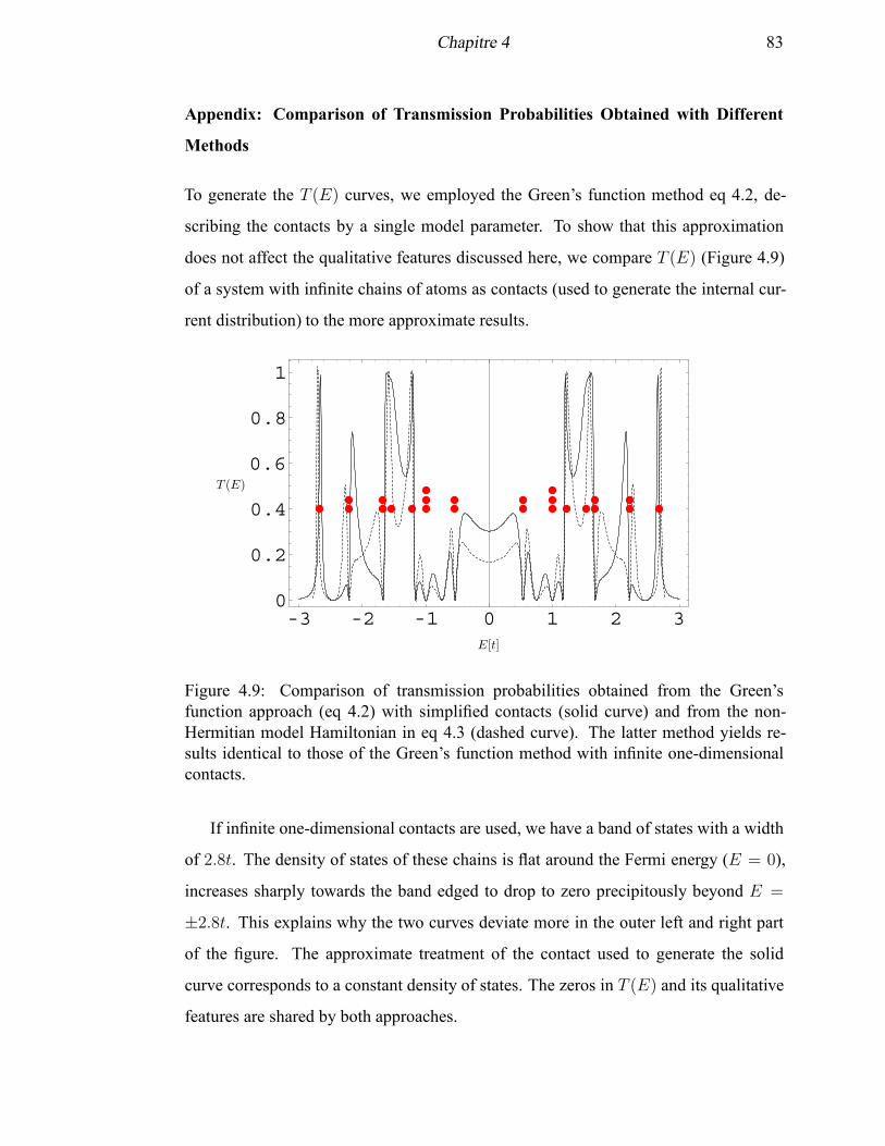
Chapitre 4 83

Appendix: Comparison of Transmission Probabilities Obtained with Different

Methods

To generate the T (E) curves, we employed the Green’s function method eq 4.2, de-

scribing the contacts by a single model parameter. To show that this approximation

does not affect the qualitative features discussed here, we compare T (E) (Figure 4.9)

of a system with infinite chains of atoms as contacts (used to generate the internal cur-

rent distribution) to the more approximate results.

-3 -2 -1 0 1 2 30

0.2

0.4

0.6

0.8

1

E[t]

T (E)

Figure 4.9: Comparison of transmission probabilities obtained from the Green’sfunction approach (eq 4.2) with simplified contacts (solid curve) and from the non-Hermitian model Hamiltonian in eq 4.3 (dashed curve). The latter method yields re-sults identical to those of the Green’s function method with infinite one-dimensionalcontacts.

If infinite one-dimensional contacts are used, we have a band of states with a width

of 2.8t. The density of states of these chains is flat around the Fermi energy (E = 0),

increases sharply towards the band edged to drop to zero precipitously beyond E =

±2.8t. This explains why the two curves deviate more in the outer left and right part

of the figure. The approximate treatment of the contact used to generate the solid

curve corresponds to a constant density of states. The zeros in T (E) and its qualitative

features are shared by both approaches.

Chapitre 4 84

4.7 Bibliography

[1] Joachim, C.; Gimzewski, J. K.; Aviram, A. Nature 2000, 408, 541-548.

[2] Nitzan, A. Annu. Rev. Phys. Chem. 2001, 52, 681-750.

[3] Nitzan, A.; Ratner, M. A. Science 2003, 300, 1384-1389.

[4] Heath, J. R.; Ratner, M. A. Phys. Today 2003, 56, 43-49.

[5] Aviram, A.; Ratner, M. A. Chem. Phys. Lett. 1974, 29, 277-283.

[6] Meir, Y.; Wingreen, N. S. Phys. Rev. Lett. 1992, 68, 2512-2515.

[7] Mujica, V.; Kemp, M.; Ratner, M. A. J. Chem. Phys. 1994, 101, 6849-6855.

[8] Datta, S. Electronic Transport in Mesoscopic Systems; Cambridge University

Press: 1995.

[9] Lang, N. D. Phys. Rev. B 1995, 52, 5335-5342.

[10] Xue, Y.; Datta, S.; Ratner, M. A. J. Chem. Phys. 2001, 115, 4292-4299.

[11] Taylor, J.; Guo, H.; Wang, J. Phys. Rev. B 2001, 63, 121104(R)/1-4.

[12] Brandbyge, M.; Mozos, J.-L.; Ordejón, P.; Taylor, J.; Stokbro, K. Phys. Rev. B

2002, 65, 165401/1-17.

[13] Ernzerhof, M.; Zhuang, M. J. Chem. Phys. 2003, 119, 4134-4140.

[14] Zhuang, M.; Rocheleau, P.; Ernzerhof, M. J. Chem. Phys. 2005, 122, 154705/1-6.

[15] Walter, D.; Neuhauser, D.; Baer, R. Chem. Phys. 2004, 299, 139-145.

[16] Sautet, P.; Joachim, C. Chem. Phys. Lett. 1988, 153, 511-516.

[17] Hod, O.; Rabani, E.; Baer, R. Acc. Chem. Res. 2006, 39, 109-117.

[18] Yi, J.; Cuniberti, G. Ann. N.Y. Acad. Sci. 2003, 1006, 306-311.

[19] Yi, J.; Cuniberti, G.; Porto, M. Eur. Phys. J. B 2003, 33, 221-225.

Chapitre 4 85

[20] Landauer, R. Philos. Mag. 1970, 21, 863-867.

[21] Cuevas, J. C.; Yeyati, A.; Martin-Rodero, A. Phys. Rev. Lett. 1998, 80, 1066-

1069.

[22] Brandbyge, M.; Kobayashi, N.; Tsukada, M. Phys. Rev. B 1999, 60, 17064-

17070.

[23] Ke, S. H.; Baranger, H.U; Yang, W. Phys. Rev. B 2003, 70, 085410/1-12.

[24] Hall, L. E.; Reimers, J. R.; Hush, N. S.; Silverbrook, K. J. Chem. Phys. 2000,

112, 1510-1521.

[25] Goyer, F.; Ernzerhof, M. Manuscript in preparation.

[26] Jackson, J. D. Classical Electrodynamics; John Wiley & Sons, Ltd.: 1998.

[27] Nakanishi, S.; Tsukada, M. Phys. Rev. Lett. 2001, 87, 126801/1-4.

[28] Mayor, M.; Didschies, C. Angew. Chem. Int. Ed. 2003, 42, 3176-3179.

[29] Aharonov, Y.; Bohm, D. Physical Review 1959, 115, 485-491.

[30] Diederich, F.; Staab, H. A. Angew. Chem. Int. Ed. 1978, 17, 372-374.

[31] Xu, B.; Xiao, X.; Yang, X.; Zang, L.; Tao, N. J. Am. Chem. Soc. 2004, 127,

2386-2387.

CHAPITRE 5

MOLECULAR CONDUCTANCE OBTAINED IN

TERMS OF ORBITAL DENSITIES AND RESPONSE

FUNCTIONS

Philippe Rocheleau and Matthias Ernzerhof



Reproduit avec la permission de Philippe Rocheleau and Matthias Ernzerhof, The

Journal of Chemical Physics, Vol. 130, 184704, (2009). Copyright 2009, American

Institute of Physics.

Chapitre 5 87


Cet article montre une application de la théorie des perturbations appliquée à l’ap-

proche « source-sink potential » (SSP) afin d’établir un lien entre certaines propriétés

moléculaires (densité et polarisabilité) et la transmission électronique des dispositifs

électroniques moléculaires (DEMs). Philippe Rocheleau a produit et rédigé l’ensemble

du contenu de l’article alors que Matthias Ernzerhof a supervisé les travaux, contribué

à l’interprétation des résultats et à la révision du manuscrit.

Chapitre 5 88

ABSTRACT

Using the source-sink potential (SSP) approach recently developed in our group,

we study electron transmission through molecular electronic devices (MEDs). Instead

of considering the source-sink potentials exactly, we use a perturbative approach to

find an expression for the transmission probability T (E) = 1 − |r(E)|2 that dependson the properties of the bare molecule. As a consequence, our approach is limited to

weak molecule-contact coupling. Provided that the orbitals of the isolated molecule

are not degenerate, we show that it is the orbital density, on the atoms that connect the

molecule to the contacts, that largely determines the transmission through the device.

Corrections to this leading-order contribution involve the second- and higher-order mo-

lecular response functions. An explicit expression for T (E) is obtained that is correct

up to first order in the molecular response function. Illustrating our approach, a qualita-

tive explanation is provided for why orders of magnitude difference in the transmission

probability are obtained [M. Mayor et al., Angew. Chem. Int. Ed. 42, 5834 (2003)]

upon modification of the contact position in the molecule. An extension of the formal-

ism to interacting systems is outlined as well.

Chapitre 5 89

5.1 Introduction

The property of interest in this article is the conductance g(E) of molecular elec-

tronic devices (MEDs)[1–5]. In an independent-electron picture, g(E) is given by the

Landauer formula [6, 7]

g(E) =e2

hT (E), (5.1)

where the transmission probability per spin channel T (E) varies between zero and one.

e2/h is the conductance quantum, i.e., the maximum conductance per spin channel.

Modeling T (E) poses a considerable challenge since the systems are infinite and non-

periodic. Here we consider a single-particle picture and comment on the interacting

case in Sec. 5.7. Furthermore, we assume that the transmission occurs in the ballistic

regime. This approximation is justified if the electron mean free path is longer than the

length of the molecule. In this article, we build on the source-sink potential approach

(SSP) [8–10] to calculate the reflection coefficient r(E) that is directly related to T (E)

by

T (E) = 1− |r(E)|2. (5.2)

We model a system for which the electrons travel from the left to the right contact.

The SSP approach takes advantage of the fact that the asymptotic behavior of the wave

function in the contacts is known. In the left contact we find for example [8],

φ(E)asymp.= φ+

L(E) + r(E)φ−

L(E). (5.3)

φ+L(E) is the right-moving Bloch wave, φ−

L(E) the reflected left-moving one and r(E)

the reflection coefficient. r(E) is a complex coefficient which we seek to determine.

Based on Eq. 5.3, in SSP, the semi-infinite contacts are replaced by artificial complex

potentials in a rigorous manner. An effective molecular Hamiltonian matrix is obtained

that emphasizes the role of the molecule in the MED, making it easier to unravel the

structure-conductance relationships. To advance this point of view, in the present contri-

bution, we pursue a perturbative approach to the molecular conductance. The complex

potentials derived from SSP are treated as a perturbation acting on the molecule. This

Chapitre 5 90

approach is justified if the complex potential is small compared to the molecular Hamil-

tonian. This is ensured by allowing only a weak coupling between the molecule and

the contacts. In this manner, we show that the key molecular properties that determine

T (E) are the orbital densities of the isolated molecule. For increased coupling between

contact and molecule, higher-order perturbative corrections have to be considered to

properly describe T (E). We derive the explicit first and second-order expressions and

demonstrate that the static orbital response function of the isolated molecule determines

the first-order correction to T (E). By static orbital response function we mean the sec-

ond derivative of the orbital energy E with respect to a perturbing one-body potential

v, i.e., δ2E/δvδv′|v=0. This response function is very similar to the polarizability as

defined in the work of Coulson and Longuet-Higgins [11] Our work enables one to

answer the question: knowing the response functions of an isolated molecule, what

can be said about the conductance that it is going to exhibit as a part of a MED? Re-

cently [12], another approach has been proposed by Yoshizawa et al. that relates the

molecular orbitals to the conductance. In contrast to our method, the one by Yoshizawa

et al. allows for a simpler account of interference effects between, for instance, the

highest occupied molecular orbital (HOMO) and lowest unoccupied molecular orbital

(LUMO). For electron energies in theMED that are in the middle of the HOMO-LUMO

gap of the isolated molecule, a superposition of HOMO and LUMO orbitals determines

the conductance. We use the contributions from individual orbitals as a starting point

and our approach is more appropriate in cases where the resonances are well separated

on the energy axis. In fact in this limit we obtain the exact answer in terms of the or-

bital densities from a simple first-order approximation. The approach by Yoshizawa et

al. and ours appear to complement each other. Pickup, Fowler, and Todorova [10, 13]

found the transmission probability of a given molecule in terms of certain character-

istic polynomials corresponding to molecular subgraphs. In combination with graph

theory these authors unravel surprising relationships between molecular structure and

conductance.

In the following Secs. 5.2-5.5, the perturbative SSP method will be discussed. As

an illustration of the theory developed here, we consider in Sec. 5.6 a recently investi-

Chapitre 5 91

gated molecule [14] that exhibits a dramatic change in the conductance as the contact

positions are changed.

5.2 Perturbative approach to the transmission probability

The system considered consists of a left contact (L) and a right contact (R) coupled

to each other by a molecule (M). The corresponding SSP Hamiltonian [8] is divided

into two contact parts, a molecular one and the coupling terms. Using an orthonormal

atomic basis, the Hamiltonian matrix is written [8] as to reflect the partitioning of the

MED into subsystems,

HSSP =

HSSPL

ML,M 0

M†L,M HM MM,R

0 M†M,R HSSP

R

, (5.4)

where MC,M (C = L or R) is a coupling matrix between contact and molecule. HSSPL

andHSSPR

describe the left and right contacts, respectively, and are given by

HSSP

L= hL +ΣL(E, r) (5.5)

and

HSSP

R = hR +ΣR(E). (5.6)

HSSPL(R)

contains a finite part of the contact explicitly through hL(R), while the complex

potentials ΣL(E, r) and ΣR(E) mimic the infinite parts of the contacts. Note that

the diagonal potential ΣL(E, r) depends on r, the quantity that we seek, and E, while

ΣR(E) depends solely onE, the energy of the incoming electron [8]. Using the Löwdin

matrix partitioning technique [15, 16], we further reduce the dimensionality of the

Hamiltonian to that of the isolated molecule. The new effective HamiltonianHeff(E, r)

(Ref. [9]) contains complex potentials ΘL(E, r) and ΘR(E), entirely replacing L and

R, respectively,

Heff(E, r) = HM −ΘL(E, r)−ΘR(E), (5.7)

Chapitre 5 92

where

ΘL(E, r) = M†L,M

[hL +ΣL(E, r)− E]−1ML,M (5.8)

and

ΘR(E) = MM,R [hR +ΣR(E)−E]−1M†

M,R. (5.9)

The artificial complex potentials ΘL(E, r) and ΘR(E) in Heff(E, r) are now treated

as perturbations of the isolated molecule. This is justified if the complex potentials

are small, i.e., if the molecule is weakly coupled to the contacts. Or alternatively, for

arbitrary perturbing potentials, the electron density in the regions of the perturbing

potential has to be small. The energy of a molecular orbital can be expressed in a

perturbation expansion with respect to the potentials ΘL(E, r) and ΘR(E). Since our

reference system is the isolated molecule that is described by a Hermitian Hamiltonian,

the perturbation expansion is the conventional one (this would not be the case [17] for

a reference Hamiltonian containing complex potentials),

E(ΘL,ΘR) =

E0 −∂E

∂ΘL

ΘL − ∂E

∂ΘR

ΘR +1

2

[

∂2E

∂Θ2L

ΘL2 + 2

∂2E

∂ΘL∂ΘR

ΘLΘR +∂2E

∂Θ2R

ΘR2

]

+ . . .

+(−1)n

n!

n∑

a=0

[

n!

a!(n− a)!

∂nE

∂ΘLa∂ΘR

(n−a)Θa

LΘ

(n−a)R

]

+ . . . . (5.10)

The energy correct to first order is given by

E(ΘL,ΘR)first order

= E0 −∂E

∂ΘL

ΘL − ∂E

∂ΘR

ΘR

= E0 − 〈Ψ|ΘL +ΘR|Ψ〉 , (5.11)

hereΨ is an unperturbed orbital. The energy correct up to second order is given by

E(ΘL,ΘR)second order

= E0 −∂E

∂ΘL

ΘL −∂E

∂ΘR

ΘR

+1

2

[

∂2E

∂Θ2L

Θ2L+ 2

∂2E

∂ΘL∂ΘR

ΘLΘR +∂2E

∂Θ2R

Θ2R

]

. (5.12)

Chapitre 5 93

In addition to density matrix elements (∂E/∂ΘL(R)), Eq. 5.12 contains the molecular

orbital response functions, i.e., ∂2E/∂ΘC ∂ΘC′ . C and C ′ can take the values L and R.

Usually, one is interested in calculating the change in energy when applying a pertur-

bation. In our case, we have a continuous energy distribution and we select an energy

at which we determine r of a particular molecular orbital. Then we use the approxi-

mation that the sum of each molecular orbital contribution to T (E) represent the full

transmission. Equations 5.11 and 5.12 are implicit expressions for r appearing in ΘL.

In Sec. 5.3, we consider the simple Hückel model and we derive explicit expressions

for r in terms of E.

5.3 Explicit expressions within the Hückel model

The contacts are represented as one-dimensional semi-infinite chains of atoms with

nearest-neighbor hopping parameter βL(R). The diagonal elements are set to zero. Build-

ing on previous work [8], we know that in the Hückel model the complex potential

ΣL(E, r) for L is given by

ΣL(E, r) = βL

e−iqL + reiqL

1 + r(5.13)

and for R it is

ΣR(E) = βReiqR. (5.14)

The interatomic coupling parameter in the semi-infinite contact is βL(R) and the wavenum-

ber of the electron is qL(R). For an infinite one-dimensional chain of atoms we can show

that [18] qL(R)(E) = arccos(E/2βL(R)) or alternatively E(qL(R)) = 2βL(R) cos(qL(R)).

Within this model, Eqs. 5.8 and 5.9 reduce to

θL(E, r) = − β2LM(1 + r)

βL(eiqL + re−iqL)(5.15)

and

θR(E) = −β2RMeiqR

βR

. (5.16)

Chapitre 5 94

βLM and βRM define the coupling of L and R with the molecule, respectively. In the

context of the Hückel model we have for the first-order correction to the energy,

E(1) = −ρLθL(E, r)− ρRθR(E). (5.17)

ρL(R) is the orbital density on the atom connected to the contact. Rearranging Eq. 5.11,

we obtain

ρLθL(E, r) = −(E −E0)− ρRθR(E). (5.18)

Because E − E0 in Eq. 5.18 is real, the imaginary part of ρLθL(E, r) must equal that

of −ρRθR(E). As a consequence, T (E) will be zero if either ρL or ρR vanishes. If

ρR vanishes but not ρL, θL(E, r) has to be real, i.e., |r|2 = 1 [9]. Furthermore, if ρL

vanishes but not ρR, a real first-order energy cannot be obtained indicating that there is

no stable state of the MED at this energy, i.e., T (E) = 0. Having a complex energy

would imply that the number of particles in the system is not conserved [8]. In case ρL

and ρR are zero, T (E) is zero because the molecular state is isolated from the contacts.

Rearranging Eqs. 5.15, 5.16, and 5.18, we get an equation for the reflection coefficient

r in the first-order approximation

r(E) =

β2LMρL

(E−E0)−β2RM

ρReiqR

βR

− βLeiqL

−β2LMρL

(E−E0)−β2RM

ρReiqR

βR

+ βLe−iqL. (5.19)

Note that this reflection coefficient is the contribution of a single orbital with energy

E0. To be able to discuss the various orbital contributions simultaneously, we add the

index i to the reflection coefficient. Furthermore, we define Ti(E) = 1 − |ri(E)|2 andapproximate T (E) ≈ ∑

i Ti(E).

Finite-order perturbation theory is always only valid within certain limits. In the

case studied here, these limits are related to the molecule-contact coupling and the

spacing between the energy levels. Criteria suitable to evaluate the validity of the finite-

order approach are based on constraints satisfied by the exact solution. For example,

we know that the transmission probability should never rise above one since we are

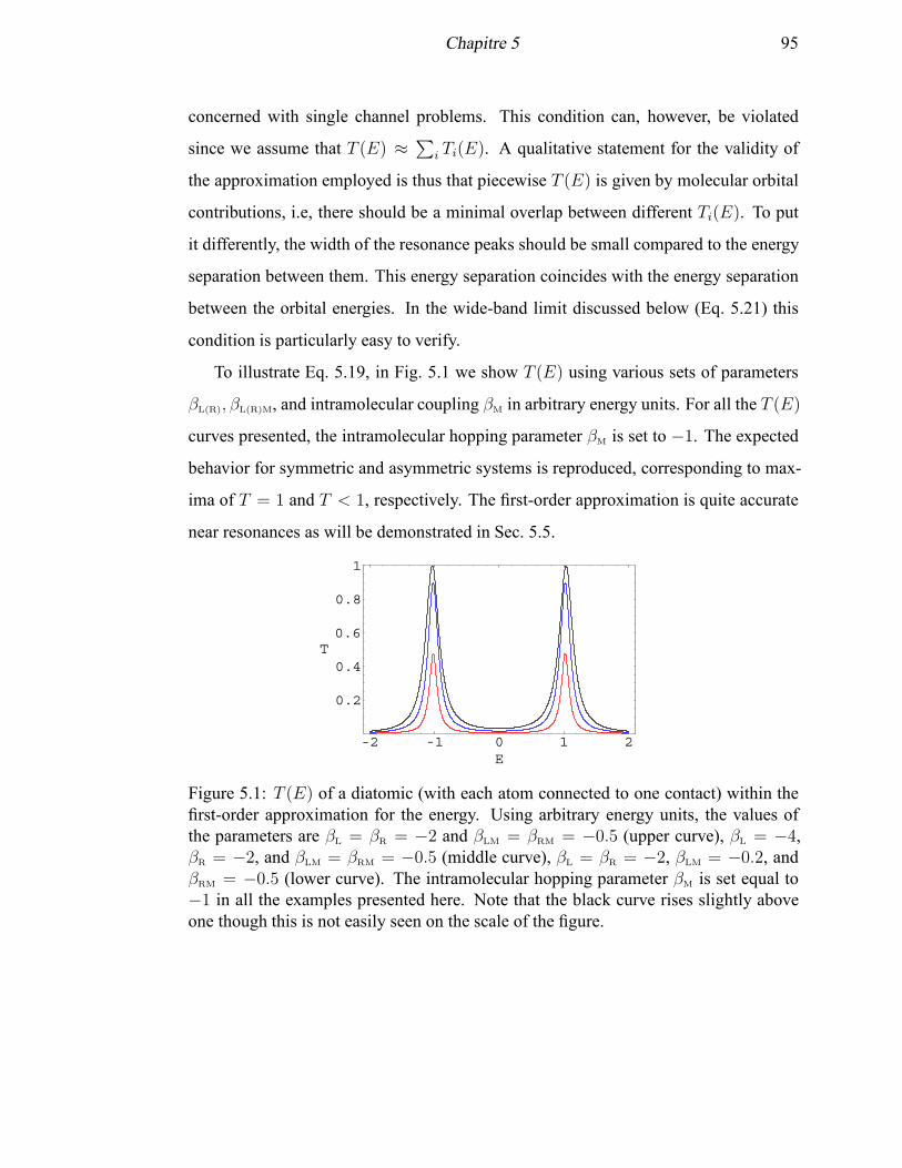
Chapitre 5 95

concerned with single channel problems. This condition can, however, be violated

since we assume that T (E) ≈∑

i Ti(E). A qualitative statement for the validity of

the approximation employed is thus that piecewise T (E) is given by molecular orbital

contributions, i.e, there should be a minimal overlap between different Ti(E). To put

it differently, the width of the resonance peaks should be small compared to the energy

separation between them. This energy separation coincides with the energy separation

between the orbital energies. In the wide-band limit discussed below (Eq. 5.21) this

condition is particularly easy to verify.

To illustrate Eq. 5.19, in Fig. 5.1 we show T (E) using various sets of parameters

βL(R), βL(R)M, and intramolecular coupling βM in arbitrary energy units. For all the T (E)

curves presented, the intramolecular hopping parameter βM is set to −1. The expected

behavior for symmetric and asymmetric systems is reproduced, corresponding to max-

ima of T = 1 and T < 1, respectively. The first-order approximation is quite accurate

near resonances as will be demonstrated in Sec. 5.5.

-2 -1 0 1 2

E

0.2

0.4

0.6

0.8

1

T

Figure 5.1: T (E) of a diatomic (with each atom connected to one contact) within thefirst-order approximation for the energy. Using arbitrary energy units, the values ofthe parameters are βL = βR = −2 and βLM = βRM = −0.5 (upper curve), βL = −4,βR = −2, and βLM = βRM = −0.5 (middle curve), βL = βR = −2, βLM = −0.2, andβRM = −0.5 (lower curve). The intramolecular hopping parameter βM is set equal to−1 in all the examples presented here. Note that the black curve rises slightly aboveone though this is not easily seen on the scale of the figure.

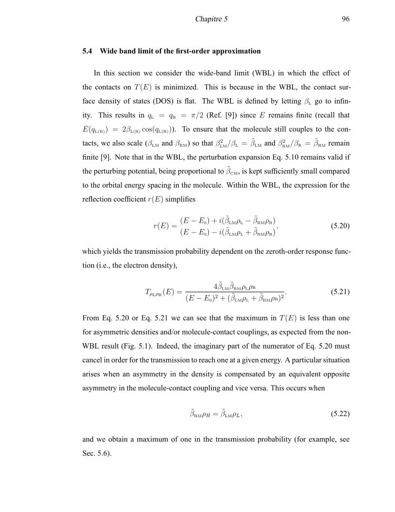
Chapitre 5 96

5.4 Wide band limit of the first-order approximation

In this section we consider the wide-band limit (WBL) in which the effect of

the contacts on T (E) is minimized. This is because in the WBL, the contact sur-

face density of states (DOS) is flat. The WBL is defined by letting βL go to infin-

ity. This results in qL = qR = π/2 (Ref. [9]) since E remains finite (recall that

E(qL(R)) = 2βL(R) cos(qL(R))). To ensure that the molecule still couples to the con-

tacts, we also scale (βLM and βRM) so that β2LM/βL = βLM and β2

RM/βR = βRM remain

finite [9]. Note that in the WBL, the perturbation expansion Eq. 5.10 remains valid if

the perturbing potential, being proportional to βCM, is kept sufficiently small compared

to the orbital energy spacing in the molecule. Within the WBL, the expression for the

reflection coefficient r(E) simplifies

r(E) =(E − E0) + i(βLMρL − βRMρR)

(E − E0)− i(βLMρL + βRMρR), (5.20)

which yields the transmission probability dependent on the zeroth-order response func-

tion (i.e., the electron density),

TρLρR(E) =4βLMβRMρLρR

(E −E0)2 + (βLMρL + βRMρR)2. (5.21)

From Eq. 5.20 or Eq. 5.21 we can see that the maximum in T (E) is less than one

for asymmetric densities and/or molecule-contact couplings, as expected from the non-

WBL result (Fig. 5.1). Indeed, the imaginary part of the numerator of Eq. 5.20 must

cancel in order for the transmission to reach one at a given energy. A particular situation

arises when an asymmetry in the density is compensated by an equivalent opposite

asymmetry in the molecule-contact coupling and vice versa. This occurs when

βRMρR = βLMρL, (5.22)

and we obtain a maximum of one in the transmission probability (for example, see

Sec. 5.6).

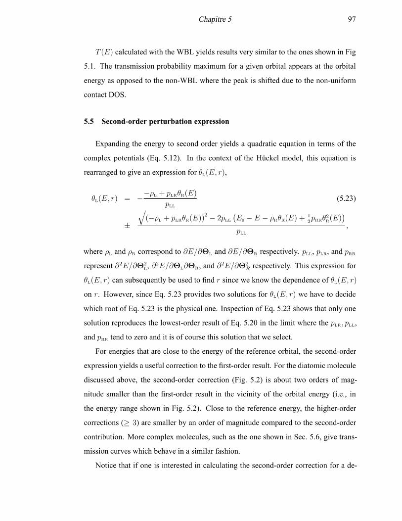
Chapitre 5 97

T (E) calculated with the WBL yields results very similar to the ones shown in Fig

5.1. The transmission probability maximum for a given orbital appears at the orbital

energy as opposed to the non-WBL where the peak is shifted due to the non-uniform

contact DOS.

5.5 Second-order perturbation expression

Expanding the energy to second order yields a quadratic equation in terms of the

complex potentials (Eq. 5.12). In the context of the Hückel model, this equation is

rearranged to give an expression for θL(E, r),

θL(E, r) = −−ρL + pLRθR(E)

pLL

(5.23)

±

√

(−ρL + pLRθR(E))2 − 2pLL

(

E0 − E − ρRθR(E) +12pRRθ2R(E)

)

pLL

,

where ρL and ρR correspond to ∂E/∂ΘL and ∂E/∂ΘR respectively. pLL, pLR, and pRR

represent ∂2E/∂Θ2L, ∂2E/∂ΘL∂ΘR, and ∂2E/∂Θ2

R respectively. This expression for

θL(E, r) can subsequently be used to find r since we know the dependence of θL(E, r)

on r. However, since Eq. 5.23 provides two solutions for θL(E, r) we have to decide

which root of Eq. 5.23 is the physical one. Inspection of Eq. 5.23 shows that only one

solution reproduces the lowest-order result of Eq. 5.20 in the limit where the pLR, pLL,

and pRR tend to zero and it is of course this solution that we select.

For energies that are close to the energy of the reference orbital, the second-order

expression yields a useful correction to the first-order result. For the diatomic molecule

discussed above, the second-order correction (Fig. 5.2) is about two orders of mag-

nitude smaller than the first-order result in the vicinity of the orbital energy (i.e., in

the energy range shown in Fig. 5.2). Close to the reference energy, the higher-order

corrections (≥ 3) are smaller by an order of magnitude compared to the second-order

contribution. More complex molecules, such as the one shown in Sec. 5.6, give trans-

mission curves which behave in a similar fashion.

Notice that if one is interested in calculating the second-order correction for a de-

Chapitre 5 98

-1.4 -1.2 -1 -0.8 -0.6

E

-0.015

-0.01

-0.005

0

0.005

0.01

0.015

0.02

T

Figure 5.2: Second-order contributions to T (E) for the lowest energy orbital of thediatomic molecule. (βL = βR = −2, βLM= βRM = −0.2, and βM = −1).

generate state, the orbital response function of the molecule becomes ill defined. In

this case, perturbation theory for degenerate states can be applied meaning that the

zeroth-order problem is redefined. By including the necessary perturbation to lift the

degeneracy, interference effects [19] in T (E) are obtained that are inaccessible by con-

ventional perturbation theory. By interference effects we refer to phenomena that are

due to the presence of at least two pathways (given here by the two degenerate orbitals)

for the electrons to traverse the molecule.

-2 -1 0 1 2

E

0

0.2

0.4

0.6

0.8

1

T

Figure 5.3: T (E) of the lowest energy orbital for a diatomic within the second-orderapproximation (βL = βR = −2 and βLM = βRM = −0.4). A tail appears to the right ofthe peak starting at E ≈ −0.5.

In Fig. 5.3 we show the second-order approximation to T (E). We obtain a main

peak and a tail that begins at E ≈ −0.5. This tail appears to be an unrealistic result of

the finite order of perturbation theory employed. If we would include the corrections up

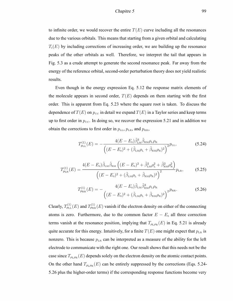
Chapitre 5 99

to infinite order, we would recover the entire T (E) curve including all the resonances

due to the various orbitals. This means that starting from a given orbital and calculating

Ti(E) by including corrections of increasing order, we are building up the resonance

peaks of the other orbitals as well. Therefore, we interpret the tail that appears in

Fig. 5.3 as a crude attempt to generate the second resonance peak. Far away from the

energy of the reference orbital, second-order perturbation theory does not yield realistic

results.

Even though in the energy expression Eq. 5.12 the response matrix elements of

the molecule appears in second order, T (E) depends on them starting with the first

order. This is apparent from Eq. 5.23 where the square root is taken. To discuss the

dependence of T (E) on pCC in detail we expand T (E) in a Taylor series and keep terms

up to first order in pCC. In doing so, we recover the expression 5.21 and in addition we

obtain the corrections to first order in pLL, pLR, and pRR,

T (1)pLL

(E) = − 4(E −E0)β3LMβRMρLρR

(

(E − E0)2 + (βLMρL + βRMρR)2)2pLL, (5.24)

T (1)pLR

(E) =4(E − E0)βLMβRM

(

(E −E0)2 + β2

LMρ2L + β2

RMρ2R

)

(

(E − E0)2 + (βLMρL + βRMρR)2)2 pLR, (5.25)

T (1)pRR

(E) = − 4(E −E0)βLMβ3RMρLρR

(

(E − E0)2 + (βLMρL + βRMρR)2)2pRR. (5.26)

Clearly, T (1)pLL(E) and T

(1)pRR(E) vanish if the electron density on either of the connecting

atoms is zero. Furthermore, due to the common factor E − E0 all three correction

terms vanish at the resonance position, implying that TρLρR(E) in Eq. 5.21 is already

quite accurate for this energy. Intuitively, for a finite T (E) one might expect that pLR is

nonzero. This is because pLR can be interpreted as a measure of the ability for the left

electrode to communicate with the right one. Our result shows that this needs not be the

case since TρLρR(E) depends solely on the electron density on the atomic contact points.

On the other hand TρLρR(E) can be entirely suppressed by the corrections (Eqs. 5.24-

5.26 plus the higher-order terms) if the corresponding response functions become very

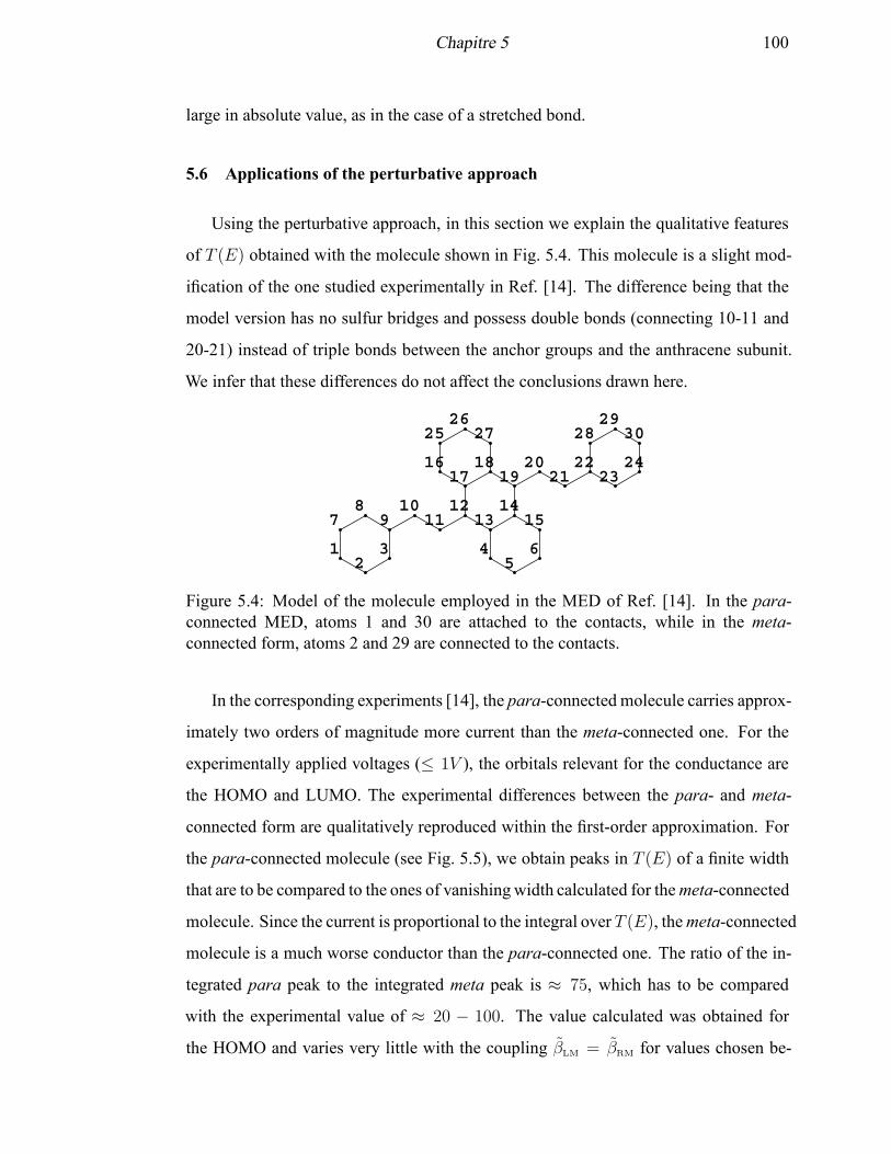
Chapitre 5 100

large in absolute value, as in the case of a stretched bond.

5.6 Applications of the perturbative approach

Using the perturbative approach, in this section we explain the qualitative features

of T (E) obtained with the molecule shown in Fig. 5.4. This molecule is a slight mod-

ification of the one studied experimentally in Ref. [14]. The difference being that the

model version has no sulfur bridges and possess double bonds (connecting 10-11 and

20-21) instead of triple bonds between the anchor groups and the anthracene subunit.

We infer that these differences do not affect the conclusions drawn here.

12

3 45

6

78

910

1112

1314

15

1617

1819

2021

2223

24

2526

27 2829

30

Figure 5.4: Model of the molecule employed in the MED of Ref. [14]. In the para-connected MED, atoms 1 and 30 are attached to the contacts, while in the meta-connected form, atoms 2 and 29 are connected to the contacts.

In the corresponding experiments [14], the para-connected molecule carries approx-

imately two orders of magnitude more current than the meta-connected one. For the

experimentally applied voltages (≤ 1V ), the orbitals relevant for the conductance are

the HOMO and LUMO. The experimental differences between the para- and meta-

connected form are qualitatively reproduced within the first-order approximation. For

the para-connected molecule (see Fig. 5.5), we obtain peaks in T (E) of a finite width

that are to be compared to the ones of vanishingwidth calculated for themeta-connected

molecule. Since the current is proportional to the integral over T (E), themeta-connected

molecule is a much worse conductor than the para-connected one. The ratio of the in-

tegrated para peak to the integrated meta peak is ≈ 75, which has to be compared

with the experimental value of ≈ 20 − 100. The value calculated was obtained for

the HOMO and varies very little with the coupling βLM = βRM for values chosen be-

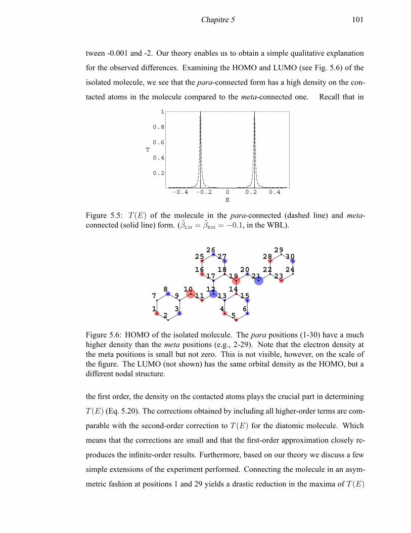
Chapitre 5 101

tween -0.001 and -2. Our theory enables us to obtain a simple qualitative explanation

for the observed differences. Examining the HOMO and LUMO (see Fig. 5.6) of the

isolated molecule, we see that the para-connected form has a high density on the con-

tacted atoms in the molecule compared to the meta-connected one. Recall that in

-0.4 -0.2 0 0.2 0.4

E

0.2

0.4

0.6

0.8

1

T

Figure 5.5: T (E) of the molecule in the para-connected (dashed line) and meta-connected (solid line) form. (βLM = βRM = −0.1, in the WBL).

12

3 45

6

78

910

1112

1314

15

1617

1819

2021

2223

24

2526

27 2829

30

Figure 5.6: HOMO of the isolated molecule. The para positions (1-30) have a muchhigher density than the meta positions (e.g., 2-29). Note that the electron density atthe meta positions is small but not zero. This is not visible, however, on the scale ofthe figure. The LUMO (not shown) has the same orbital density as the HOMO, but adifferent nodal structure.

the first order, the density on the contacted atoms plays the crucial part in determining

T (E) (Eq. 5.20). The corrections obtained by including all higher-order terms are com-

parable with the second-order correction to T (E) for the diatomic molecule. Which

means that the corrections are small and that the first-order approximation closely re-

produces the infinite-order results. Furthermore, based on our theory we discuss a few

simple extensions of the experiment performed. Connecting the molecule in an asym-

metric fashion at positions 1 and 29 yields a drastic reduction in the maxima of T (E)

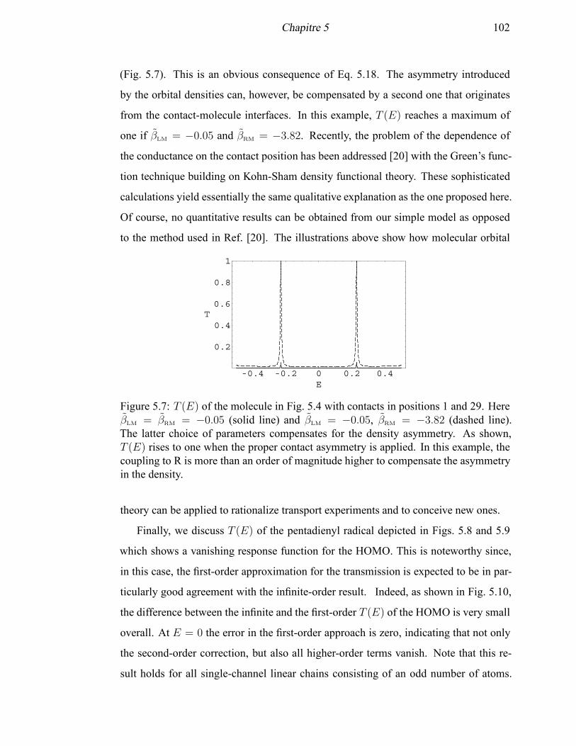
Chapitre 5 102

(Fig. 5.7). This is an obvious consequence of Eq. 5.18. The asymmetry introduced

by the orbital densities can, however, be compensated by a second one that originates

from the contact-molecule interfaces. In this example, T (E) reaches a maximum of

one if βLM = −0.05 and βRM = −3.82. Recently, the problem of the dependence of

the conductance on the contact position has been addressed [20] with the Green’s func-

tion technique building on Kohn-Sham density functional theory. These sophisticated

calculations yield essentially the same qualitative explanation as the one proposed here.

Of course, no quantitative results can be obtained from our simple model as opposed

to the method used in Ref. [20]. The illustrations above show how molecular orbital

-0.4 -0.2 0 0.2 0.4

E

0.2

0.4

0.6

0.8

1

T

Figure 5.7: T (E) of the molecule in Fig. 5.4 with contacts in positions 1 and 29. HereβLM = βRM = −0.05 (solid line) and βLM = −0.05, βRM = −3.82 (dashed line).The latter choice of parameters compensates for the density asymmetry. As shown,T (E) rises to one when the proper contact asymmetry is applied. In this example, thecoupling to R is more than an order of magnitude higher to compensate the asymmetryin the density.

theory can be applied to rationalize transport experiments and to conceive new ones.

Finally, we discuss T (E) of the pentadienyl radical depicted in Figs. 5.8 and 5.9

which shows a vanishing response function for the HOMO. This is noteworthy since,

in this case, the first-order approximation for the transmission is expected to be in par-

ticularly good agreement with the infinite-order result. Indeed, as shown in Fig. 5.10,

the difference between the infinite and the first-order T (E) of the HOMO is very small

overall. At E = 0 the error in the first-order approach is zero, indicating that not only

the second-order correction, but also all higher-order terms vanish. Note that this re-

sult holds for all single-channel linear chains consisting of an odd number of atoms.

Chapitre 5 103

1

2

3

4

5

Figure 5.8: HOMO of the pentadienyl radical. This orbital has a vanishing responsefunction if connected in the 1-5 position. Notice that both connecting atoms have alarge electron density.

-2 -1 0 1 20.0

0.2

0.4

0.6

0.8

1.0

E

T

Figure 5.9: First-order approximation to T (E) for the pentadienyl radical. (βLM =βRM = −0.02, in the WBL).

Conductance oscillations in linear wires are a well studied phenomenon (see, e.g. [21]

and references therein) and the pentadienyl molecule is an example of a single-channel

conductor with an odd number of atoms. In the zero-voltage limit these odd-numbered

atomic wires show a conductance maximum of one at the Fermi energy which is zero

in our example. The fact that the molecular response function in the Hückel approxi-

mation is zero indicates that the resonance at the Fermi energy is robust with respect to

perturbations.

5.7 Extension to an interacting system

It is possible to extend the perturbative SSP approach to an interactingMED, permit-

ting an account of correlation effects within the molecule. In this section, we describe

how this can be accomplished. We imagine a MED in the zero-voltage limit where

an electron travels through L with an energy equal to the Fermi energy. This electron

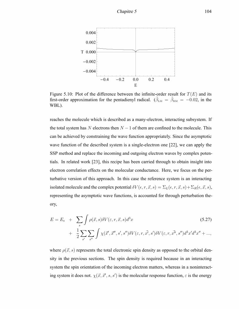
Chapitre 5 104

-0.4 -0.2 0.0 0.2 0.4

-0.004

-0.002

0.000

0.002

0.004

E

T

Figure 5.10: Plot of the difference between the infinite-order result for T (E) and itsfirst-order approximation for the pentadienyl radical. (βLM = βRM = −0.02, in theWBL).

reaches the molecule which is described as a many-electron, interacting subsystem. If

the total system hasN electrons thenN − 1 of them are confined to the molecule. This

can be achieved by constraining the wave function appropriately. Since the asymptotic

wave function of the described system is a single-electron one [22], we can apply the

SSP method and replace the incoming and outgoing electron waves by complex poten-

tials. In related work [23], this recipe has been carried through to obtain insight into

electron correlation effects on the molecular conductance. Here, we focus on the per-

turbative version of this approach. In this case the reference system is an interacting

isolated molecule and the complex potential δV (ǫ, r, ~x, s) = ΣL(ǫ, r, ~x, s)+ΣR(ǫ, ~x, s),

representing the asymptotic wave functions, is accounted for through perturbation the-

ory,

E = E0 +∑

s

∫

ρ(~x, s)δV (ε, r, ~x, s)d3x (5.27)

+1

2

∑

s′

∑

s′′

∫

χ(~x′, ~x′′, s′, s′′)δV (ε, r, ~x′, s′)δV (ε, r, ~x′′, s′′)d3x′d3x′′ + ...,

where ρ(~x, s) represents the total electronic spin density as opposed to the orbital den-

sity in the previous sections. The spin density is required because in an interacting

system the spin orientation of the incoming electron matters, whereas in a noninteract-

ing system it does not. χ(~x, ~x′, s, s′) is the molecular response function, ε is the energy

Chapitre 5 105

of the inserted electron, s is the spin index and E0 is the total energy of the system

unperturbed by the complex potentials. The total energy of the interacting system E

can be separated into two contributions [22],

E = EN−1 + ε, (5.28)

where EN−1 is the energy of the MED with one electron removed such that N − 1 elec-

trons remain at the molecule. As before, we seek r in the complex potential. Choosing

a certain ǫ and E, we find it from Eq. 5.27. Since now, the correlated electron density

and response function determine r, correlation effects in the molecule are accounted

for. Other examples where the transmission probability is related to the spin density of

the molecular subsystem can be found in the pioneering paper by Meir and Wingreen

[24]. In their treatment of the Kondo effect, the electron density on the quantum dot de-

termines T (E) exactly. Note that the exact density and not its nth order approximation

is required in the theory of Ref. [24].

It is well known that conductance calculations based on Kohn-Sham density func-

tional theory in conjunction with local and semilocal functionals tends to overestimate

T (E) [25, 26]. Equation 5.27 helps to understand this tendency. Since approximate

density functionals yield an electron density that is too diffuse and delocalized, the cou-

pling to the external contacts tends to be overestimated. In the weakly coupled limit,

our approach allows for a complete account of correlation effects in the molecule if the

molecular response functions are available.

5.8 Conclusions

To take advantage of the intuitive understanding of molecular orbitals in the area

of molecular electronics, we treat the isolated molecule as our reference system and

we introduce the external contacts in a newly developed perturbative fashion. We find

that the orbital densities are the deciding factor in the first-order transmission proba-

bility and furthermore, we find that the first-order contribution is the dominant one to

T (E) if the resonances are separated. Our first-order approach mirrors the qualitative

Chapitre 5 106

concept according to which each molecular orbital (assuming it is connected to the con-

tacts) yields a resonance in T (E). We also identify a clear limitation of this concept

which appears for degenerate orbitals. Considering recent experiments [14], we show

that our approach offers a simple, molecular-orbital-based explanation for the observed

behavior. Furthermore, at least in principle, the simple molecular orbital picture can

be extended in a systematic fashion to account for higher-order corrections to T (E).

We find that the second-order correction is determined by the orbital response function,

another molecular property that is well understood. The qualitative approach presented

here is intended as a conceptual tool for the interpretation and conception of experi-

ments in molecular electronics. Clearly it has its limitations in cases where there is

a strong overlap of orbital resonances. Such problems can be dealt with using another

qualitative approach proposed recently [12] that is particularly useful in the cases where

several orbitals contribute simultaneously to the transmission probability.

Acknowledgments

We gratefully acknowledge financial support provided by NSERC.

5.9 Bibliography

[1] C. Joachim, J. K. Ginzewski, and A. Aviram, Nature (London) 408, 541 (2000).



[4] J. R. Heath and M. A. Ratner, Phys. Today 56(5), 43 (2003).

[5] F. Chen, J. Hihath, Z. Huang, X. Li, and N. J. Tao, Annu. Rev. Phys. Chem. 58,

535 (2007).

[6] Y. Imry and R. Landauer, Rev. Mod. Phys. 71, S306 (1999).

[7] R. Landauer, Philos. Mag. 21, 863 (1970).

Chapitre 5 107

[8] F. Goyer, M. Ernzerhof, and M. Zhuang, J. Chem. Phys. 126, 144104 (2007).

[9] M. Ernzerhof, J. Chem. Phys. 127, 204709 (2007).

[10] B. T. Pickup and P. W. Fowler, Chem. Phys. Lett. 459, 198 (2008).

[11] C. A. Coulson and H. C. Longuet-Higgins, Proc. R. Soc. London, Ser. A 191, 39

(1947).

[12] K. Yoshizawa, T. Tada, and A. Staykov, J. Am. Chem. Soc. 130, 9406 (2008).

[13] P. W. Fowler, B. T. Pickup, and T. Todorova, Chem. Phys. Lett. 465, 142 (2008).

[14] M. Mayor, H. B. Weber, J. Reichert, M. Elbing, C. von Hanisch, D. Beckmann,

and M. Fischer, Angew. Chem. Int. Ed. 42, 5834 (2003).

[15] P. O. Löwdin, J. Math. Phys. 3, 969 (1962).

[16] P. O. Löwdin, J. Mol. Spectrosc. 10, 12 (1963).

[17] C. Buth, R. Santra, and L. S. Cederbaum, Phys. Rev. A 69, 032505 (2004).

[18] N. W. Ashcroft and N. D. Mermin, Solid State Physics (Saunders, Philadelphia,

1976).

[19] M. Ernzerhof, H. Bahmann, F. Goyer, M. Zhuang, and P. Rocheleau, J. Chem.

Theory Comput. 2, 1291 (2006).

[20] Y. Y. Liang, Y. X. Zhou, H. Chen, R. Note, H. Mizuseki, and Y. Kawazoe, J. Chem.

Phys. 129, 024901 (2008).

[21] M. Zhuang and M. Ernzerhof, J. Chem. Phys. 120, 4921 (2004).

[22] J. Katriel and E. R. Davidson, Proc. Natl. Acad. Sci. USA 77, 4403 (1980).

[23] A. Goker, F. Goyer, and M. Ernzerhof, J. Chem. Phys. 129, 194901 (2008).


[25] M. Ernzerhof and M. Zhuang, Int. J. Quantum Chem. 101, 557 (2005).

Chapitre 5 108

[26] M. Koentopp, K. Burke, and F. Evers, Phys. Rev. B 73, 121403 (2006).

CHAPITRE 6

EXTENSION OF THE SOURCE-SINK POTENTIAL

(SSP) APPROACH TOMULTICHANNEL QUANTUM

TRANSPORT

Philippe Rocheleau and Matthias Ernzerhof



Reproduit avec la permission de Philippe Rocheleau and Matthias Ernzerhof, The

Journal of Chemical Physics, Vol. 137, 174112, (2012). Copyright 2012, American

Institute of Physics.

Chapitre 6 110


Cet article présente une extension à plusieurs canaux de transmission de la méthode

« source-sink potential » (SSP) pour la transmission électronique de dispositifs élec-

troniques moléculaires (DEMs). Philippe Rocheleau a produit et rédigé l’ensemble du

contenu de l’article alors que Matthias Ernzerhof a supervisé les travaux, contribué à

l’interprétation des résultats et à la révision du manuscrit.

Chapitre 6 111

ABSTRACT

We present an extension of the single channel source-sink potential (SSP) approach

[F. Goyer, M. Ernzerhof, and M. Zhuang, J. Chem. Phys. 126, 144104 (2007)] for

molecular electronic devices (MEDs) to multiple channels. The proposed multichannel

source-sink potential method relies on an eigenchannel description of conducting states

of the MED which are obtained by a self-consistent algorithm. We use the newly devel-

oped model to examine the transport of the 1-phenyl-1,3-butadiene molecule connected

to two coupled rows of atoms that act as contacts on the left and right sides. With an

eigenchannel description of the wave function in the contacts, we determined that one

of the eigenchannels is effectively closed by the interference effects of the side chain.

Furthermore, we provide an example where we observe a complete inversion (from

bonding to antibonding and vice versa) of the transverse character of the wave function

upon passage through the molecule.

Chapitre 6 112

6.1 Introduction

In molecular electronics, molecules are attached to macroscopic contacts [1–5].

Much of the theoretical work about molecular electronic devices (MEDs) involves the

use of Green’s function theory [6–8] for ballistic transport. Another theory to describe

MEDs is the source-sink potential (SSP) approach [9], which allows one to relate the

structure of the molecule to its conducting properties by analyzing the wave functions.

Most of the work involving SSP is done within the Hückel approximation [10–13] and

we believe that much can be learned from such simple models. Other workers follow

similar lines, Fowler, Pickup, Todorova, and co-workers [14–17] developed simple ex-

pressions for the molecular conductance within the Hückel/SSP model and presented

numerous rules [18, 19] for its prediction. Recently Ratner, Reuter, Solomon, and co-

workers explored various aspect of multichannel transport [20] by considering a small

coupling between two single channel molecular conductors [21, 22]. Their work is

based on a Green’s function approach [6, 8, 23] applied within a tight-binding model.

Many articles that discuss multichannel phenomena within the Green’s function ap-

proach are based on work presented in Ref. [24]. Other authors discuss multichannel

problems within scattering theory [25–28]. Furthermore, inelastic processes, involving,

for example, interacting electrons and phonons, necessitate a multichannel description

(see, e.g., Ref. [29]).

In this contribution, we extend the single channel SSP method to multiple channels.

We provide the wave functions that correspond to the conducting eigenchannels in con-

trast to various other works that report the total transmission probability. Other articles

that discuss eigenchannels are often based on the work presented in Refs. [24, 26] and

[30]. Recently Dumont addressed the multichannel problem within SSP [31]. He pro-

posed an elegant solution that explicitly deals with electron transfer from one channel

to another. We choose a different route here by proposing an eigenchannel approach

which is expected to be generalizable to the more sophisticated electronic structure

theory methods, such as density functional theory (DFT) and configuration interaction

(CI). Indeed, in previous publications [32, 33], DFT and CI have been combined with

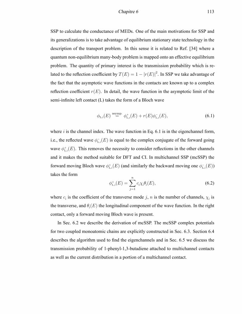
Chapitre 6 113

SSP to calculate the conductance of MEDs. One of the main motivations for SSP and

its generalizations is to take advantage of equilibrium stationary state technology in the

description of the transport problem. In this sense it is related to Ref. [34] where a

quantum non-equilibriummany-body problem is mapped onto an effective equilibrium

problem. The quantity of primary interest is the transmission probability which is re-

lated to the reflection coefficient by T (E) = 1− |r(E)|2. In SSP we take advantage ofthe fact that the asymptotic wave functions in the contacts are known up to a complex

reflection coefficient r(E). In detail, the wave function in the asymptotic limit of the

semi-infinite left contact (L) takes the form of a Bloch wave

φL,i(E)asymp.= φ+

L,i(E) + r(E)φ−

L,i(E), (6.1)

where i is the channel index. The wave function in Eq. 6.1 is in the eigenchannel form,

i.e., the reflected wave φ−

L,i(E) is equal to the complex conjugate of the forward going

wave φ+L,i(E). This removes the necessity to consider reflections in the other channels

and it makes the method suitable for DFT and CI. In multichannel SSP (mcSSP) the

forward moving Bloch wave φ+L,i(E) (and similarly the backward moving one φ−

L,i(E))

takes the form

φ+

L,i(E) =

n∑

j=1

cjχjθj(E), (6.2)

where cj is the coefficient of the transverse mode j, n is the number of channels, χj is

the transverse, and θj(E) the longitudinal component of the wave function. In the right

contact, only a forward moving Bloch wave is present.

In Sec. 6.2 we describe the derivation of mcSSP. The mcSSP complex potentials

for two coupled monoatomic chains are explicitly constructed in Sec. 6.3. Section 6.4

describes the algorithm used to find the eigenchannels and in Sec. 6.5 we discuss the

transmission probability of 1-phenyl-1,3-butadiene attached to multichannel contacts

as well as the current distribution in a portion of a multichannel contact.

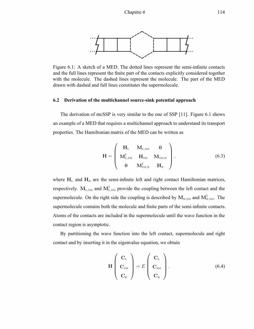
Chapitre 6 114

Figure 6.1: A sketch of a MED. The dotted lines represent the semi-infinite contactsand the full lines represent the finite part of the contacts explicitly considered togetherwith the molecule. The dashed lines represent the molecule. The part of the MEDdrawn with dashed and full lines constitutes the supermolecule.

6.2 Derivation of the multichannel source-sink potential approach

The derivation of mcSSP is very similar to the one of SSP [11]. Figure 6.1 shows

an example of a MED that requires a multichannel approach to understand its transport

properties. The Hamiltonian matrix of the MED can be written as

H =

HL ML,SM 0

M†L,SM HSM MSM,R

0 M†SM,R HR

, (6.3)

where HL and HR are the semi-infinite left and right contact Hamiltonian matrices,

respectively. ML,SM and M†L,SM provide the coupling between the left contact and the

supermolecule. On the right side the coupling is described by MR,SM and M†R,SM. The

supermolecule contains both the molecule and finite parts of the semi-infinite contacts.

Atoms of the contacts are included in the supermolecule until the wave function in the

contact region is asymptotic.

By partitioning the wave function into the left contact, supermolecule and right

contact and by inserting it in the eigenvalue equation, we obtain

H

CL

CSM

CR

= E

CL

CSM

CR

. (6.4)

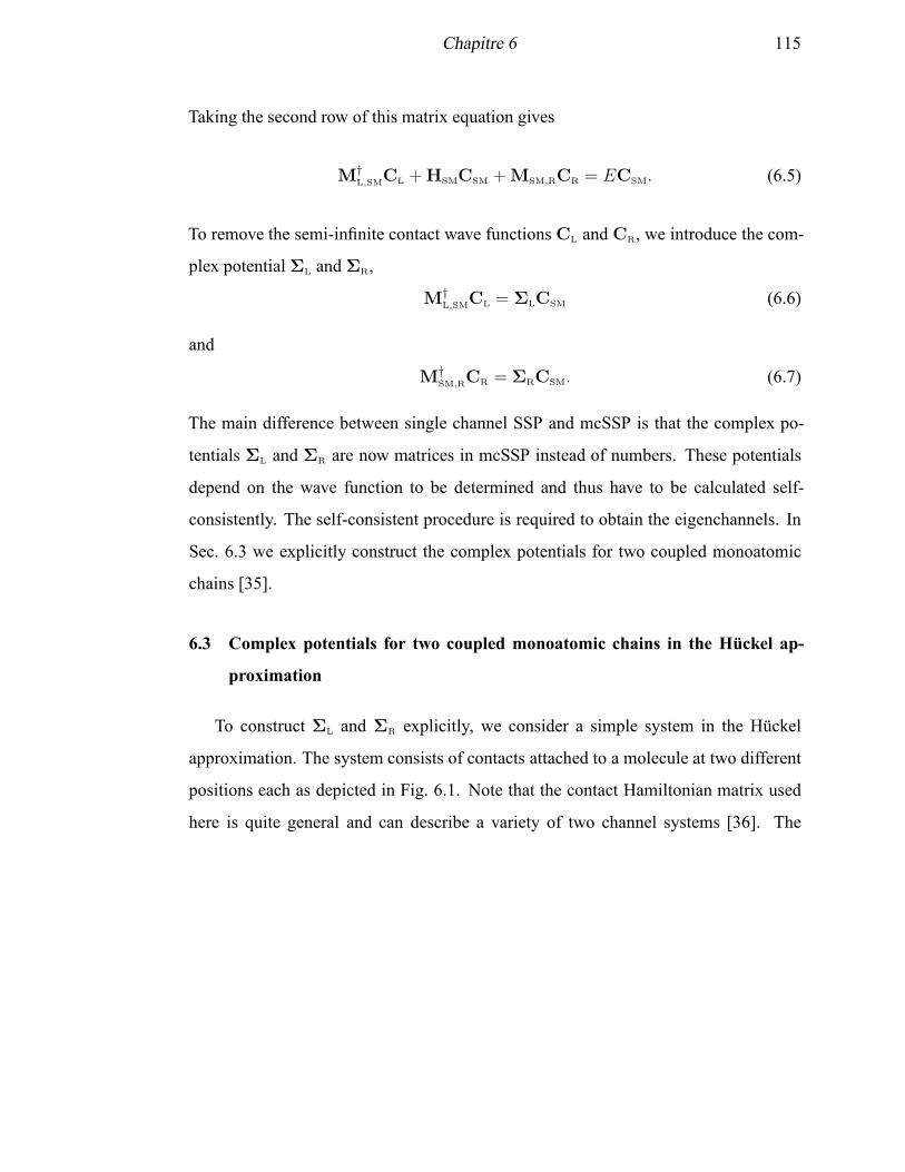
Chapitre 6 115

Taking the second row of this matrix equation gives

M†L,SMCL +HSMCSM +MSM,RCR = ECSM. (6.5)

To remove the semi-infinite contact wave functions CL and CR, we introduce the com-

plex potential ΣL and ΣR,

M†L,SMCL = ΣLCSM (6.6)

and

M†SM,RCR = ΣRCSM. (6.7)

The main difference between single channel SSP and mcSSP is that the complex po-

tentials ΣL and ΣR are now matrices in mcSSP instead of numbers. These potentials

depend on the wave function to be determined and thus have to be calculated self-

consistently. The self-consistent procedure is required to obtain the eigenchannels. In

Sec. 6.3 we explicitly construct the complex potentials for two coupled monoatomic

chains [35].

6.3 Complex potentials for two coupled monoatomic chains in the Hückel ap-

proximation

To construct ΣL and ΣR explicitly, we consider a simple system in the Hückel

approximation. The system consists of contacts attached to a molecule at two different

positions each as depicted in Fig. 6.1. Note that the contact Hamiltonian matrix used

here is quite general and can describe a variety of two channel systems [36]. The

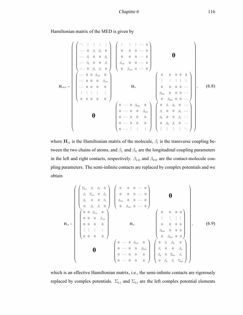
Chapitre 6 116

Hamiltonian matrix of the MED is given by

HMED =

. . ....

......

...

· · · 0 βt βL 0

· · · βt 0 0 βL

· · · βL 0 0 βt

· · · 0 βL βt 0

......

... · · · 0

0 0 0 · · · 0

0 0 0 · · · 0

βLM 0 0 · · · 0

0 βLM 0 · · · 0

0

· · · 0 0 βLM 0

· · · 0 0 0 βLM

· · · 0 0 0 0...

......

......

0 0 0 0 0

HM

0 0 0 0 0...

......

......

0 0 0 0 · · ·βRM 0 0 0 · · ·0 βRM 0 0 · · ·

0

0 · · · 0 βRM 0

0 · · · 0 0 βRM

0 · · · 0 0 0

0 · · · 0 0 0

0 · · · ......

...

0 βt βR 0 · · ·βt 0 0 βR · · ·βR 0 0 βt · · ·0 βR βt 0 · · ·...

......

.... . .

, (6.8)

where HM is the Hamiltonian matrix of the molecule, βt is the transverse coupling be-

tween the two chains of atoms, and βL and βR are the longitudinal coupling parameters

in the left and right contacts, respectively. βLM and βRM are the contact-molecule cou-

pling parameters. The semi-infinite contacts are replaced by complex potentials and we

obtain

Heff =

ΣL1 βt βL 0

βt ΣL2 0 βL

βL 0 0 βt

0 βL βt 0

0 0 0 · · · 0

0 0 0 · · · 0

βLM 0 0 · · · 0

0 βLM 0 · · · 0

0

0 0 βLM 0

0 0 0 βLM

0 0 0 0...

......

...

0 0 0 0

HM

0 0 0 0...

......

...

0 0 0 0

βRM 0 0 0

0 βRM 0 0

0

0 · · · 0 βRM 0

0 · · · 0 0 βRM

0 · · · 0 0 0

0 · · · 0 0 0

0 βt βR 0

βt 0 0 βR

βR 0 ΣR1 βt

0 βR βt ΣR2

, (6.9)

which is an effective Hamiltonian matrix, i.e., the semi-infinite contacts are rigorously

replaced by complex potentials. ΣL1 and ΣL2 are the left complex potential elements

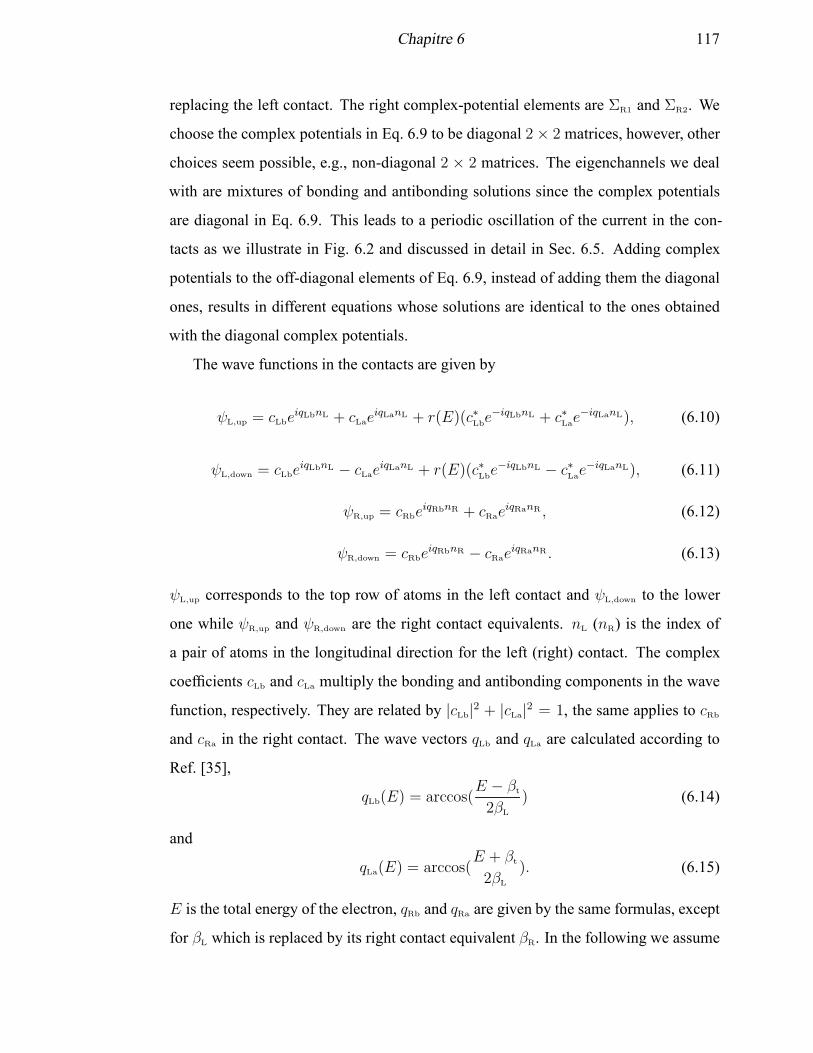
Chapitre 6 117

replacing the left contact. The right complex-potential elements are ΣR1 and ΣR2. We

choose the complex potentials in Eq. 6.9 to be diagonal 2× 2 matrices, however, other

choices seem possible, e.g., non-diagonal 2 × 2 matrices. The eigenchannels we deal

with are mixtures of bonding and antibonding solutions since the complex potentials

are diagonal in Eq. 6.9. This leads to a periodic oscillation of the current in the con-

tacts as we illustrate in Fig. 6.2 and discussed in detail in Sec. 6.5. Adding complex

potentials to the off-diagonal elements of Eq. 6.9, instead of adding them the diagonal

ones, results in different equations whose solutions are identical to the ones obtained

with the diagonal complex potentials.

The wave functions in the contacts are given by

ψL,up = cLbeiqLbnL + cLae

iqLanL + r(E)(c∗Lbe−iqLbnL + c∗Lae

−iqLanL), (6.10)

ψL,down = cLbeiqLbnL − cLae

iqLanL + r(E)(c∗Lbe−iqLbnL − c∗Lae

−iqLanL), (6.11)

ψR,up = cRbeiqRbnR + cRae

iqRanR , (6.12)

ψR,down = cRbeiqRbnR − cRae

iqRanR. (6.13)

ψL,up corresponds to the top row of atoms in the left contact and ψL,down to the lower

one while ψR,up and ψR,down are the right contact equivalents. nL (nR) is the index of

a pair of atoms in the longitudinal direction for the left (right) contact. The complex

coefficients cLb and cLa multiply the bonding and antibonding components in the wave

function, respectively. They are related by |cLb|2 + |cLa|2 = 1, the same applies to cRb

and cRa in the right contact. The wave vectors qLb and qLa are calculated according to

Ref. [35],

qLb(E) = arccos(E − βt

2βL

) (6.14)

and

qLa(E) = arccos(E + βt

2βL

). (6.15)

E is the total energy of the electron, qRb and qRa are given by the same formulas, except

for βL which is replaced by its right contact equivalent βR. In the following we assume

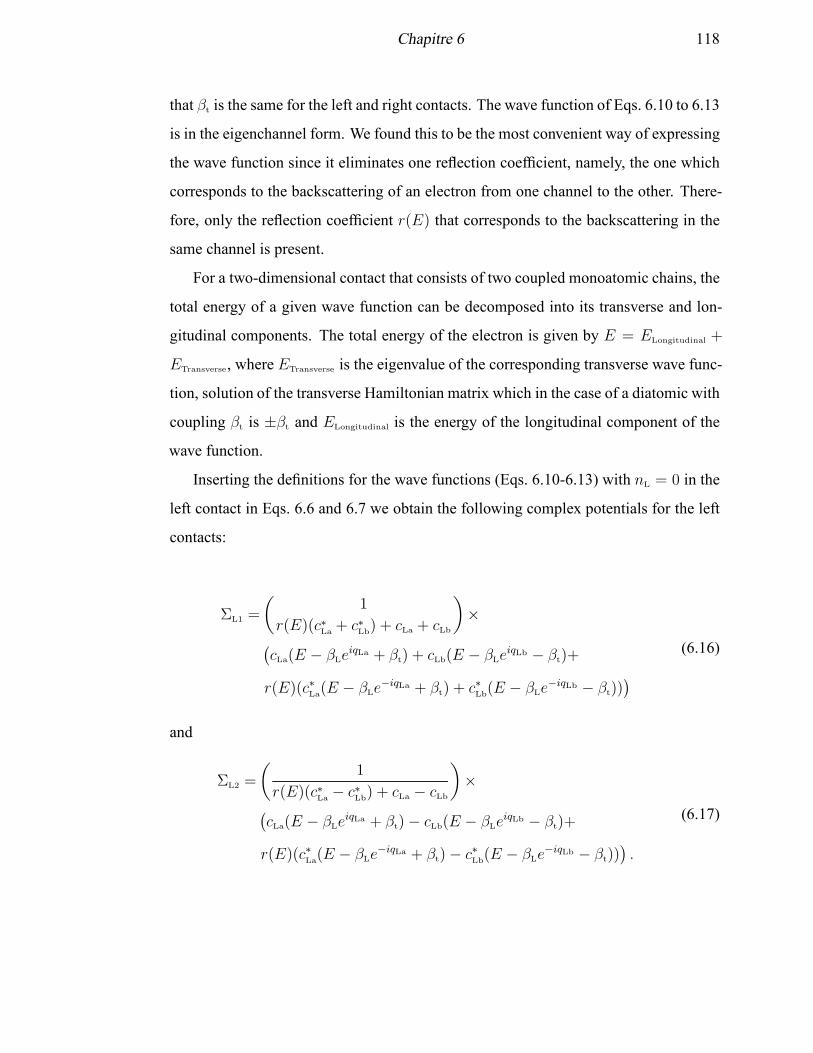
Chapitre 6 118

that βt is the same for the left and right contacts. The wave function of Eqs. 6.10 to 6.13

is in the eigenchannel form. We found this to be the most convenient way of expressing

the wave function since it eliminates one reflection coefficient, namely, the one which

corresponds to the backscattering of an electron from one channel to the other. There-

fore, only the reflection coefficient r(E) that corresponds to the backscattering in the

same channel is present.

For a two-dimensional contact that consists of two coupled monoatomic chains, the

total energy of a given wave function can be decomposed into its transverse and lon-

gitudinal components. The total energy of the electron is given by E = ELongitudinal +

ETransverse, where ETransverse is the eigenvalue of the corresponding transverse wave func-

tion, solution of the transverse Hamiltonian matrix which in the case of a diatomic with

coupling βt is ±βt and ELongitudinal is the energy of the longitudinal component of the

wave function.

Inserting the definitions for the wave functions (Eqs. 6.10-6.13) with nL = 0 in the

left contact in Eqs. 6.6 and 6.7 we obtain the following complex potentials for the left

contacts:

ΣL1 =

(

1

r(E)(c∗La+ c∗

Lb) + cLa + cLb

)

×(

cLa(E − βLeiqLa + βt) + cLb(E − βLe

iqLb − βt)+

r(E)(c∗La(E − βLe−iqLa + βt) + c∗Lb(E − βLe

−iqLb − βt)))

(6.16)

and

ΣL2 =

(

1

r(E)(c∗La − c∗Lb) + cLa − cLb

)

×(

cLa(E − βLeiqLa + βt)− cLb(E − βLe

iqLb − βt)+

r(E)(c∗La(E − βLe

−iqLa + βt)− c∗Lb(E − βLe

−iqLb − βt)))

.

(6.17)

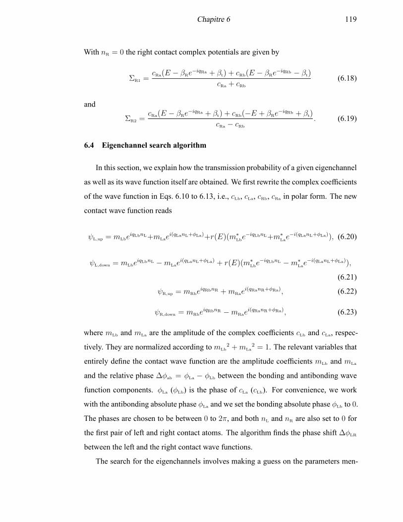
Chapitre 6 119

With nR = 0 the right contact complex potentials are given by

ΣR1 =cRa(E − βRe

−iqRa + βt) + cRb(E − βRe−iqRb − βt)

cRa + cRb

(6.18)

and

ΣR2 =cRa(E − βRe

−iqRa + βt) + cRb(−E + βRe−iqRb + βt)

cRa − cRb

. (6.19)

6.4 Eigenchannel search algorithm

In this section, we explain how the transmission probability of a given eigenchannel

as well as its wave function itself are obtained. We first rewrite the complex coefficients

of the wave function in Eqs. 6.10 to 6.13, i.e., cLb, cLa, cRb, cRa in polar form. The new

contact wave function reads

ψL,up = mLbeiqLbnL+mLae

i(qLanL+φLa)+r(E)(m∗Lbe−iqLbnL+m∗

Lae−i(qLanL+φLa)), (6.20)

ψL,down = mLbeiqLbnL −mLae

i(qLanL+φLa) + r(E)(m∗Lbe−iqLbnL −m∗

Lae−i(qLanL+φLa)),

(6.21)

ψR,up = mRbeiqRbnR +mRae

i(qRanR+φRa), (6.22)

ψR,down = mRbeiqRbnR −mRae

i(qRanR+φRa), (6.23)

where mLb and mLa are the amplitude of the complex coefficients cLb and cLa, respec-

tively. They are normalized according tomLb2 +mLa

2 = 1. The relevant variables that

entirely define the contact wave function are the amplitude coefficients mLb and mLa

and the relative phase ∆φab = φLa − φLb between the bonding and antibonding wave

function components. φLa (φLb) is the phase of cLa (cLb). For convenience, we work

with the antibonding absolute phase φLa and we set the bonding absolute phase φLb to 0.

The phases are chosen to be between 0 to 2π, and both nL and nR are also set to 0 for

the first pair of left and right contact atoms. The algorithm finds the phase shift ∆φLR

between the left and the right contact wave functions.

The search for the eigenchannels involves making a guess on the parameters men-

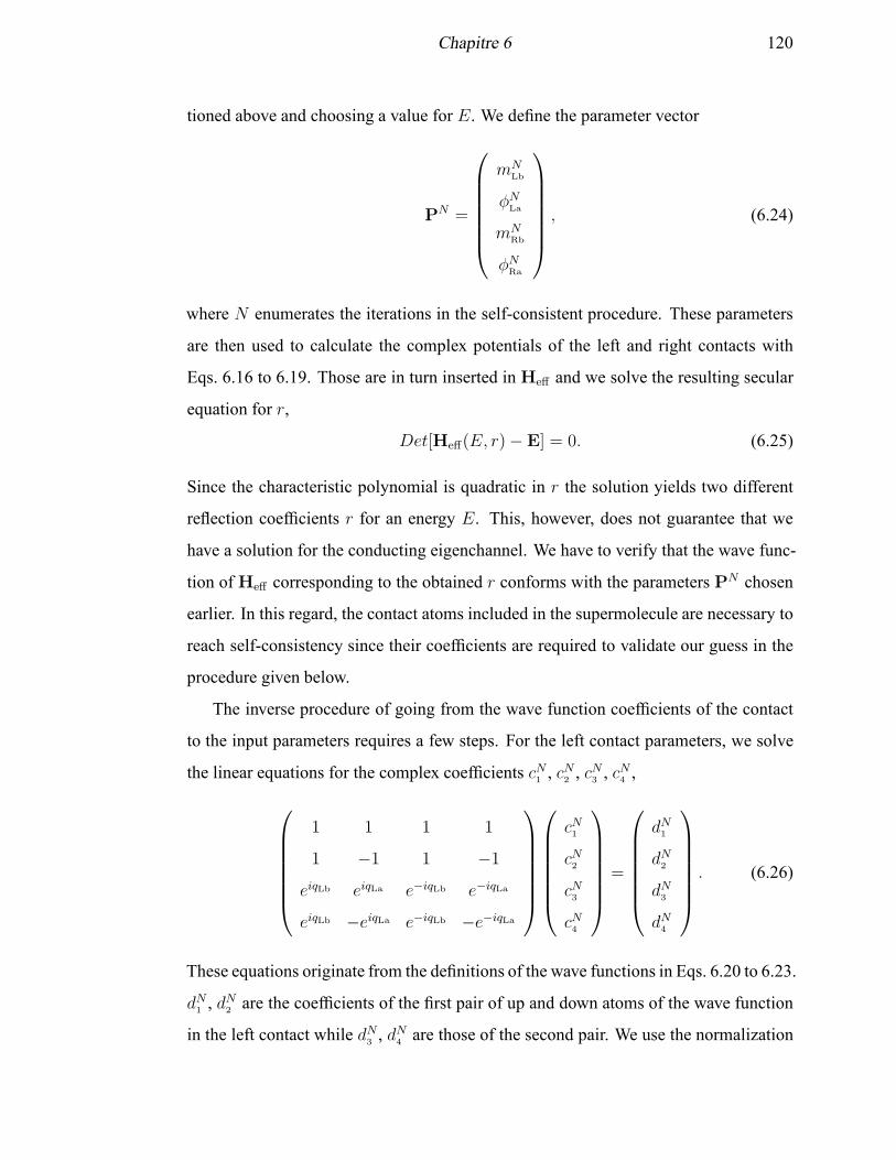
Chapitre 6 120

tioned above and choosing a value for E. We define the parameter vector

PN =

mNLb

φNLa

mNRb

φNRa

, (6.24)

where N enumerates the iterations in the self-consistent procedure. These parameters

are then used to calculate the complex potentials of the left and right contacts with

Eqs. 6.16 to 6.19. Those are in turn inserted inHeff and we solve the resulting secular

equation for r,

Det[Heff(E, r)− E] = 0. (6.25)

Since the characteristic polynomial is quadratic in r the solution yields two different

reflection coefficients r for an energy E. This, however, does not guarantee that we

have a solution for the conducting eigenchannel. We have to verify that the wave func-

tion ofHeff corresponding to the obtained r conforms with the parameters PN chosen

earlier. In this regard, the contact atoms included in the supermolecule are necessary to

reach self-consistency since their coefficients are required to validate our guess in the

procedure given below.

The inverse procedure of going from the wave function coefficients of the contact

to the input parameters requires a few steps. For the left contact parameters, we solve

the linear equations for the complex coefficients cN1, cN

2, cN

3, cN

4,

1 1 1 1

1 −1 1 −1

eiqLb eiqLa e−iqLb e−iqLa

eiqLb −eiqLa e−iqLb −e−iqLa

cN1

cN2

cN3

cN4

=

dN1

dN2

dN3

dN4

. (6.26)

These equations originate from the definitions of the wave functions in Eqs. 6.20 to 6.23.

dN1 , dN2 are the coefficients of the first pair of up and down atoms of the wave function

in the left contact while dN3, dN

4are those of the second pair. We use the normalization

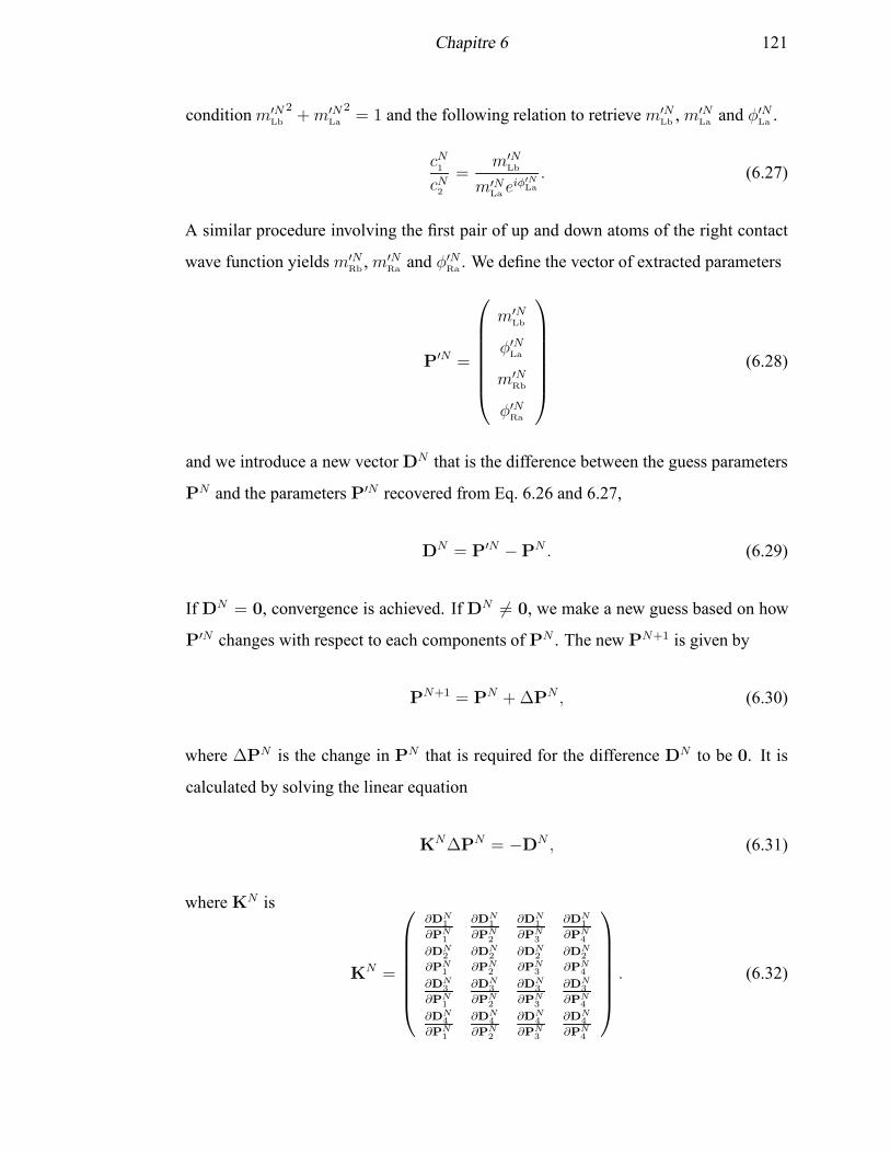
Chapitre 6 121

conditionm′NLb

2+m′N

La

2= 1 and the following relation to retrievem′N

Lb ,m′NLa and φ

′NLa .

cN1

cN2

=m′N

Lb

m′NLaeiφ

′NLa

. (6.27)

A similar procedure involving the first pair of up and down atoms of the right contact

wave function yieldsm′NRb,m′N

Raand φ′N

Ra. We define the vector of extracted parameters

P′N =

m′NLb

φ′NLa

m′NRb

φ′NRa

(6.28)

and we introduce a new vectorDN that is the difference between the guess parameters

PN and the parameters P′N recovered from Eq. 6.26 and 6.27,

DN = P′N −PN . (6.29)

If DN = 0, convergence is achieved. If DN 6= 0, we make a new guess based on how

P′N changes with respect to each components of PN . The new PN+1 is given by

PN+1 = PN +∆PN , (6.30)

where ∆PN is the change in PN that is required for the difference DN to be 0. It is

calculated by solving the linear equation

KN∆PN = −DN , (6.31)

whereKN is

KN =

∂DN1

∂PN1

∂DN1

∂PN2

∂DN1

∂PN3

∂DN1

∂PN4

∂DN2

∂PN1

∂DN2

∂PN2

∂DN2

∂PN3

∂DN2

∂PN4

∂DN3

∂PN1

∂DN3

∂PN2

∂DN3

∂PN3

∂DN3

∂PN4

∂DN4

∂PN1

∂DN4

∂PN2

∂DN4

∂PN3

∂DN4

∂PN4

. (6.32)

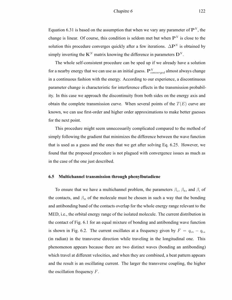
Chapitre 6 122

Equation 6.31 is based on the assumption that when we vary any parameter of PN , the

change is linear. Of course, this condition is seldom met but when PN is close to the

solution this procedure converges quickly after a few iterations. ∆PN is obtained by

simply inverting theKN matrix knowing the difference in parametersDN .

The whole self-consistent procedure can be sped up if we already have a solution

for a nearby energy that we can use as an initial guess. PNconverged almost always change

in a continuous fashion with the energy. According to our experience, a discontinuous

parameter change is characteristic for interference effects in the transmission probabil-

ity. In this case we approach the discontinuity from both sides on the energy axis and

obtain the complete transmission curve. When several points of the T (E) curve are

known, we can use first-order and higher order approximations to make better guesses

for the next point.

This procedure might seem unnecessarily complicated compared to the method of

simply following the gradient that minimizes the difference between the wave function

that is used as a guess and the ones that we get after solving Eq. 6.25. However, we

found that the proposed procedure is not plagued with convergence issues as much as

in the case of the one just described.

6.5 Multichannel transmission through phenylbutadiene

To ensure that we have a multichannel problem, the parameters βL, βR, and βt of

the contacts, and βM of the molecule must be chosen in such a way that the bonding

and antibonding band of the contacts overlap for the whole energy range relevant to the

MED, i.e., the orbital energy range of the isolated molecule. The current distribution in

the contact of Fig. 6.1 for an equal mixture of bonding and antibonding wave function

is shown in Fig. 6.2. The current oscillates at a frequency given by F = qLb − qLa

(in radian) in the transverse direction while traveling in the longitudinal one. This

phenomenon appears because there are two distinct waves (bonding an antibonding)

which travel at different velocities, and when they are combined, a beat pattern appears

and the result is an oscillating current. The larger the transverse coupling, the higher

the oscillation frequency F .

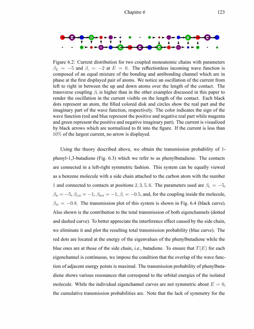
Chapitre 6 123

Figure 6.2: Current distribution for two coupled monoatomic chains with parametersβL = −5 and βt = −2 at E = 0. The reflectionless incoming wave function iscomposed of an equal mixture of the bonding and antibonding channel which are inphase at the first displayed pair of atoms. We notice an oscillation of the current fromleft to right in between the up and down atoms over the length of the contact. Thetransverse coupling βt is higher than in the other examples discussed in this paper torender the oscillation in the current visible on the length of the contact. Each blackdots represent an atom, the filled colored disk and circles show the real part and theimaginary part of the wave function, respectively. The color indicates the sign of thewave function (red and blue represent the positive and negative real part while magentaand green represent the positive and negative imaginary part). The current is visualizedby black arrows which are normalized to fit into the figure. If the current is less than10% of the largest current, no arrow is displayed.

Using the theory described above, we obtain the transmission probability of 1-

phenyl-1,3-butadiene (Fig. 6.3) which we refer to as phenylbutadiene. The contacts

are connected in a left-right symmetric fashion. This system can be equally viewed

as a benzene molecule with a side chain attached to the carbon atom with the number

1 and connected to contacts at positions 2, 3, 5, 6. The parameters used are βL = −5,

βR = −5, βLM = −1, βRM = −1, βt = −0.5, and, for the coupling inside the molecule,

βM = −0.8. The transmission plot of this system is shown in Fig. 6.4 (black curve).

Also shown is the contribution to the total transmission of both eigenchannels (dotted

and dashed curve). To better appreciate the interference effect caused by the side chain,

we eliminate it and plot the resulting total transmission probability (blue curve). The

red dots are located at the energy of the eigenvalues of the phenylbutadiene while the

blue ones are at those of the side chain, i.e., butadiene. To ensure that T (E) for each

eigenchannel is continuous, we impose the condition that the overlap of the wave func-

tion of adjacent energy points is maximal. The transmission probability of phenylbuta-

diene shows various resonances that correspond to the orbital energies of the isolated

molecule. While the individual eigenchannel curves are not symmetric about E = 0,

the cumulative transmission probabilities are. Note that the lack of symmetry for the

Chapitre 6 124

1

2

3

4

5

6

7

8

9

10

Figure 6.3: Carbon backbone of the phenylbutadiene molecule. For convenience thecarbon atoms are enumerated.

individual eigenchannels is the consequence of the choice of having smoothly chang-

ing eigenchannel wave functions. Destructive interferences are visible at E ≈ −1.3

and E ≈ −0.45, one for each eigenchannel, and they correspond to orbital energies

of the isolated side chain. The total transmission maximum of T ≈ 2 occurs at the

degenerate orbitals energy E = −0.8 for benzene and at E ≈ −0.95 with T ≈ 1.6 for

phenylbutadiene. This difference is caused by the side chain that breaks the degeneracy

of the benzene orbitals, the orbital that couples to the butadiene moves to a lower energy

while the other remain unperturbed. To verify our results, we also calculated the trans-

mission probabilities with the Green’s function approach and found agreement. If more

channels are available at a given energy we expect the total transmission to be higher.

However, an inspection of Fig. 6.4 near the destructive interference at E ≈ −1.3 re-

veals that the first eigenchannel (dotted line) is completely shut while the second one

is open with T ≈ 1. In Fig. 6.5 we show the device orbitals (DOs) at E = −1.31, the

first orbital describes an electron that is backscattered in the left contact to yield a stand-

ing wave whereas the second orbital carries current and is mostly bonding in character.

The region between E = −0.8 and E = −1 contains two orbitals of the phenylbutadi-

ene molecule. Those are the two degenerate orbitals of benzene, one of which moved

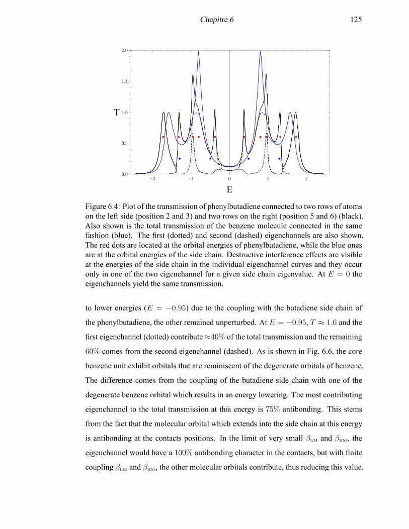
Chapitre 6 125

-2 -1 0 1 20.0

0.5

1.0

1.5

2.0

E

T

Figure 6.4: Plot of the transmission of phenylbutadiene connected to two rows of atomson the left side (position 2 and 3) and two rows on the right (position 5 and 6) (black).Also shown is the total transmission of the benzene molecule connected in the samefashion (blue). The first (dotted) and second (dashed) eigenchannels are also shown.The red dots are located at the orbital energies of phenylbutadiene, while the blue onesare at the orbital energies of the side chain. Destructive interference effects are visibleat the energies of the side chain in the individual eigenchannel curves and they occuronly in one of the two eigenchannel for a given side chain eigenvalue. At E = 0 theeigenchannels yield the same transmission.

to lower energies (E = −0.95) due to the coupling with the butadiene side chain of

the phenylbutadiene, the other remained unperturbed. At E = −0.95, T ≈ 1.6 and the

first eigenchannel (dotted) contribute≈40% of the total transmission and the remaining

60% comes from the second eigenchannel (dashed). As is shown in Fig. 6.6, the core

benzene unit exhibit orbitals that are reminiscent of the degenerate orbitals of benzene.

The difference comes from the coupling of the butadiene side chain with one of the

degenerate benzene orbital which results in an energy lowering. The most contributing

eigenchannel to the total transmission at this energy is 75% antibonding. This stems

from the fact that the molecular orbital which extends into the side chain at this energy

is antibonding at the contacts positions. In the limit of very small βLM and βRM, the

eigenchannel would have a 100% antibonding character in the contacts, but with finite

coupling βLM and βRM, the other molecular orbitals contribute, thus reducing this value.

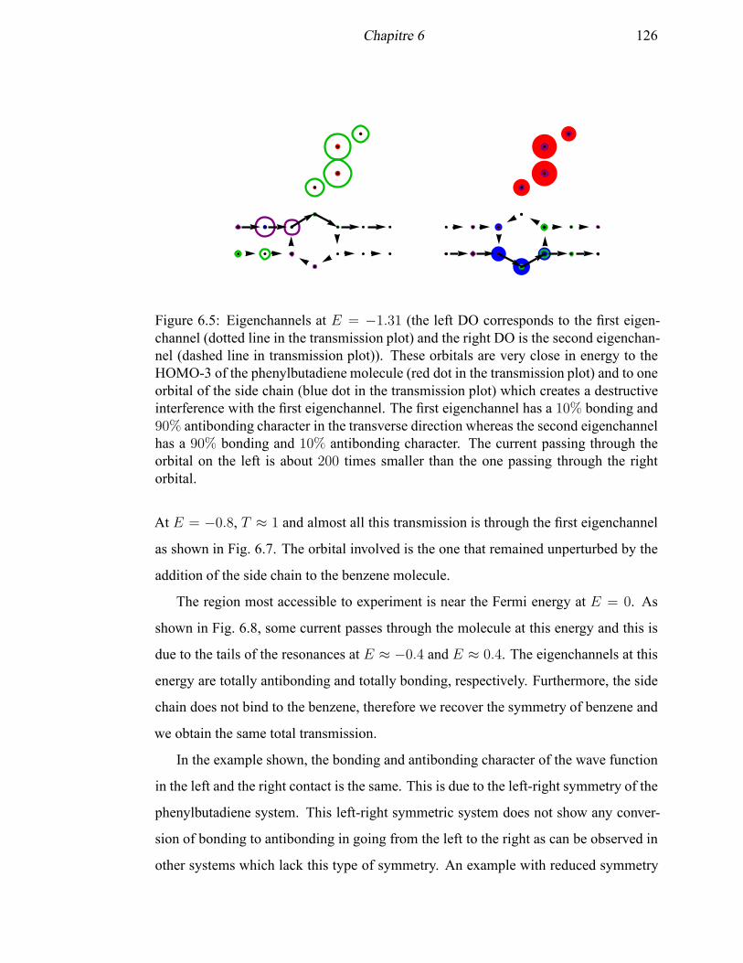
Chapitre 6 126

Figure 6.5: Eigenchannels at E = −1.31 (the left DO corresponds to the first eigen-channel (dotted line in the transmission plot) and the right DO is the second eigenchan-nel (dashed line in transmission plot)). These orbitals are very close in energy to theHOMO-3 of the phenylbutadiene molecule (red dot in the transmission plot) and to oneorbital of the side chain (blue dot in the transmission plot) which creates a destructiveinterference with the first eigenchannel. The first eigenchannel has a 10% bonding and90% antibonding character in the transverse direction whereas the second eigenchannelhas a 90% bonding and 10% antibonding character. The current passing through theorbital on the left is about 200 times smaller than the one passing through the rightorbital.

At E = −0.8, T ≈ 1 and almost all this transmission is through the first eigenchannel

as shown in Fig. 6.7. The orbital involved is the one that remained unperturbed by the

addition of the side chain to the benzene molecule.

The region most accessible to experiment is near the Fermi energy at E = 0. As

shown in Fig. 6.8, some current passes through the molecule at this energy and this is

due to the tails of the resonances at E ≈ −0.4 and E ≈ 0.4. The eigenchannels at this

energy are totally antibonding and totally bonding, respectively. Furthermore, the side

chain does not bind to the benzene, therefore we recover the symmetry of benzene and

we obtain the same total transmission.

In the example shown, the bonding and antibonding character of the wave function

in the left and the right contact is the same. This is due to the left-right symmetry of the

phenylbutadiene system. This left-right symmetric system does not show any conver-

sion of bonding to antibonding in going from the left to the right as can be observed in

other systems which lack this type of symmetry. An example with reduced symmetry

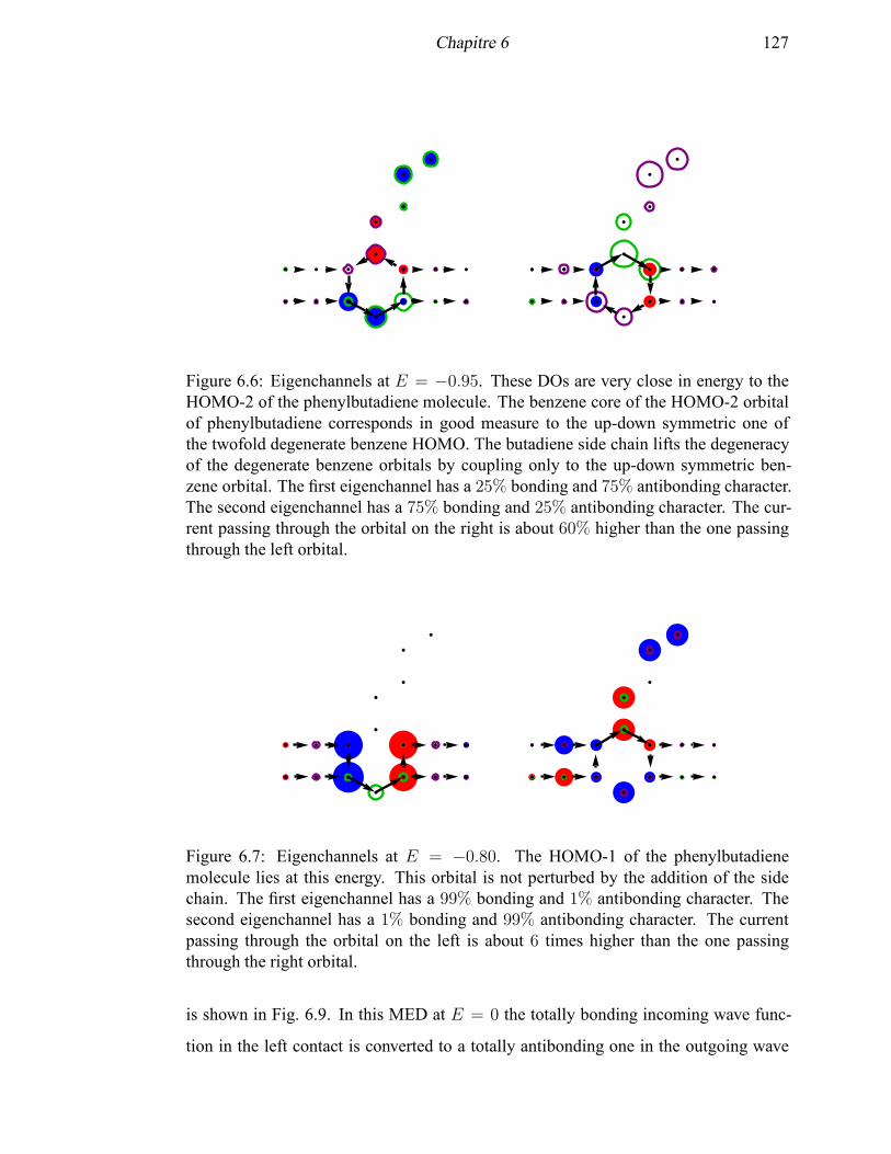
Chapitre 6 127

Figure 6.6: Eigenchannels at E = −0.95. These DOs are very close in energy to theHOMO-2 of the phenylbutadiene molecule. The benzene core of the HOMO-2 orbitalof phenylbutadiene corresponds in good measure to the up-down symmetric one ofthe twofold degenerate benzene HOMO. The butadiene side chain lifts the degeneracyof the degenerate benzene orbitals by coupling only to the up-down symmetric ben-zene orbital. The first eigenchannel has a 25% bonding and 75% antibonding character.The second eigenchannel has a 75% bonding and 25% antibonding character. The cur-rent passing through the orbital on the right is about 60% higher than the one passingthrough the left orbital.

Figure 6.7: Eigenchannels at E = −0.80. The HOMO-1 of the phenylbutadienemolecule lies at this energy. This orbital is not perturbed by the addition of the sidechain. The first eigenchannel has a 99% bonding and 1% antibonding character. Thesecond eigenchannel has a 1% bonding and 99% antibonding character. The currentpassing through the orbital on the left is about 6 times higher than the one passingthrough the right orbital.

is shown in Fig. 6.9. In this MED at E = 0 the totally bonding incoming wave func-

tion in the left contact is converted to a totally antibonding one in the outgoing wave

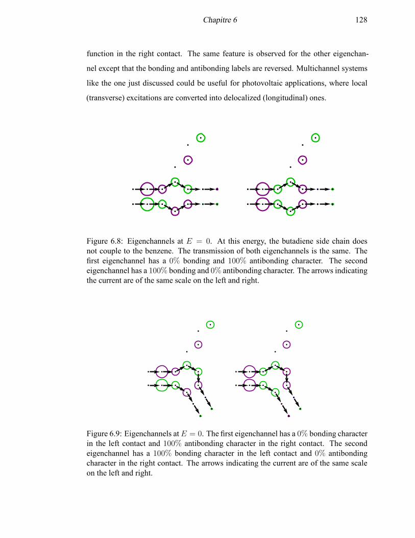
Chapitre 6 128

function in the right contact. The same feature is observed for the other eigenchan-

nel except that the bonding and antibonding labels are reversed. Multichannel systems

like the one just discussed could be useful for photovoltaic applications, where local

(transverse) excitations are converted into delocalized (longitudinal) ones.

Figure 6.8: Eigenchannels at E = 0. At this energy, the butadiene side chain doesnot couple to the benzene. The transmission of both eigenchannels is the same. Thefirst eigenchannel has a 0% bonding and 100% antibonding character. The secondeigenchannel has a 100% bonding and 0% antibonding character. The arrows indicatingthe current are of the same scale on the left and right.

Figure 6.9: Eigenchannels atE = 0. The first eigenchannel has a 0% bonding characterin the left contact and 100% antibonding character in the right contact. The secondeigenchannel has a 100% bonding character in the left contact and 0% antibondingcharacter in the right contact. The arrows indicating the current are of the same scaleon the left and right.

Chapitre 6 129

6.6 Conclusion

The original version of the SSP approach is limited to single channel problems.

To overcome this restriction, Dumont [31] developed an extension to the multichannel

case, by extending the number of outgoing channels. Deviating from this approach, our

theory reduces the multichannel problem to effective single channel ones. This means

that we calculate the eigenchannels iteratively, one at a time. In the past we employed

single channel SSP in conjunction with the configuration interaction method [37] and

density functional theory [32]. Similarly, the state specific method developed here

is expected to be compatible with CI and DFT. While Green’s function theory [6–8]

offers an elegant and complete solution to the non-equilibrium transport problem, fully

implementing it for interacting electrons remains a formidable challenge. Therefore it

appears to be useful to search for alternatives that permit the use of the existing density

functional and wave function technology. Furthermore, our mcSSP approach allows for

a detailed analysis of the multichannel transport problem. As the examples show, the

transport mechanism can be discussed comprehensively and explained largely in terms

of single channel phenomena. A new element of the multichannel theory, not present

in the single channel case, is the transformation of transverse into longitudinal energy

(and vice versa) upon passage through the molecule. This effect might be exploitable

in photovoltaic cells where energy is transferred from localized to delocalized degrees

of freedom.

Acknowledgments

The authors are grateful for the financial support provided by NSERC.

Chapitre 6 130

6.7 Bibliography

[1] C. Joachim, J. K. Gimzewski, and A. Aviram, Nature(London) 408, 541 (2000).



[4] J. R. Heath and M. A. Ratner, Phys. Today 56(5), 43 (2003).

[5] F. Chen, J. Hihath, Z. Huang, X. Li, and N. J. Tao, Annu. Rev. Phys. Chem. 58,

535 (2007).



[8] S. Datta, Electronic Transport in Mesoscopic Systems (Cambridge University

Press, Cambridge, England, 1995).

[9] F. Goyer, M. Ernzerhof, and M. Zhuang, J. Chem. Phys. 126, 144104 (2007).

[10] M. Ernzerhof, M. Zhuang, and P. Rocheleau, J. Chem. Phys. 123, 134704 (2005).


[12] P. Rocheleau and M. Ernzerhof, J. Chem. Phys. 130, 184704 (2009).


[14] P. W. Fowler, B. T. Pickup, and T. Z. Todorova, Pure Appl. Chem. 83, 1515

(2011).

[15] P. W. Fowler, B. T. Pickup, T. Z. Todorova, and T. Pisanski, J. Chem. Phys. 130,

174708 (2009).

[16] P. W. Fowler, B. T. Pickup, and T. Z. Todorova, Chem. Phys. Lett. 465, 142

(2008).

[17] B. T. Pickup and P. W. Fowler, Chem. Phys. Lett. 459, 198 (2008).

Chapitre 6 131

[18] P. W. Fowler, B. T. Pickup, T. Z. Todorova, and W. Myrvold, J. Chem. Phys. 131,

044104 (2009).

[19] P. W. Fowler, B. T. Pickup, T. Z. Todorova, and W. Myrvold, J. Chem. Phys. 131,

244110 (2009).

[20] M. Buttiker, Y. Imry, R. Landauer, and S. Pinhas, Phys. Rev. B 31, 6207 (1985).

[21] M. G. Reuter, G. C. Solomon, T. Hansen, T. Seideman, and M. A. Ratner, J. Phys.

Chem. Lett. 2, 1667 (2011).

[22] M. G. Reuter, M. C. Hersam, T. Seideman, and M. A. Ratner, Nano Letters 12,

2243 (2012).

[23] Y. Xue, S. Datta, and M. A. Ratner, Chem. Phys. 281, 151 (2002).

[24] M. Paulsson and M. Brandbyge, Phys. Rev. B 76, 115117 (2007).

[25] P. J. Price, Phys. Rev. B 48, 17301 (1993).

[26] M. Brandbyge, M. R. Sorensen, and K. W. Jacobsen, Phys. Rev. B 56, 14956

(1997).

[27] A. Bagrets, N. Papanikolaou, and I. Mertig, Phys. Rev. B 75, 235448 (2007).

[28] D. Mencarelli, T. Rozzi, and L. Pierantoni, Nanotechnology 21, 155701 (2010).

[29] J. Bonca and S. A. Trugman, Phys. Rev. Lett. 75, 2566 (1995).

[30] D. Jacob and J. J. Palacios, Phys. Rev. B 73, 075429 (2006).

[31] R. S. Dumont, J. Chem. Phys. 134, 044119 (2011).

[32] Y. Zhou and M. Ernzerhof, J. Chem. Phys. 136, 094105 (2012).

[33] Y. Zhou and M. Ernzerhof, J. Phys. Chem. Lett. 3, 1916 (2012).

[34] J. E. Han, Phys. Rev. B 73, 125319 (2006).

[35] R. Farchioni, G. Grosso, and G. P. Parravicini, Eur. Phys. J. B 84, 227 (2011).

Chapitre 6 132

[36] P. Darancet, V. Olevano, and D. Mayou, Phys. Rev. B 81, 155422 (2010).

[37] F. Goyer and M. Ernzerhof, J. Chem. Phys. 134, 174101 (2011).

CONCLUSION

7.1 Synthèse et discussion générale des résultats

La miniaturisation constante et l’intégration toujours de plus en plus importante des

dispositifs électroniques nous rapprochent inlassablement vers la limite fondamentale

de la taille de ces unités. À l’échelle nanométrique, les effets quantiques dominent, ce

qui nécessite un changement d’approche pour le développement et la compréhension

de ces dispositifs. Étudier le phénomène de transport d’électrons à cette échelle repré-

sente un défi important [1] pour plusieurs raisons. D’une part, au niveau expérimental

les équipements doivent être de plus en plus perfectionnés et précis pour caractériser les

systèmes à l’échelle nanométrique [2]. De plus, il est difficile de déterminer la structure

exacte des systèmes étudiés. Au niveau théorique, les méthodes doivent être adaptées

et les modèles doivent inclure les composantes importantes pour décrire le système en

question. Une des difficultés rencontrées dans l’étude des DEMs est que le système est

composé de parties infinies comme les contacts et également d’une partie finie, la mo-

lécule. Ceci rend la modélisation plus difficile puisque les techniques habituelles qui

consistent à utiliser les conditions frontière périodiques et celle qui consiste à utiliser

des fonctions de base localisées sont difficilement applicables. Les travaux initiaux sur

les DEMs ont porté dans un premier temps sur les nanofils [3–5] de métaux tels que

l’aluminium, le sodium [6] et l’or [7–9]. Bien que l’aspect des nanofils soit toujours

d’intérêt, une grande attention est portée sur les dispositifs qui intègrent un aspect mo-

léculaire (DEM) au système afin d’en modifier les caractéristiques de transport.

Dans cette thèse, chaque chapitre traite d’un aspect particulier des DEMs. Une grande

partie des travaux présentés concernent le développement de la méthode SSP [10], la-

quelle a été pour la première fois décrite en détail en 2007. Depuis, elle est constam-

ment améliorée et elle nous a permis de mieux comprendre les DEMs et en particulier,

Conclusion 134

d’étudier certaines relations entre la transmission et la structure moléculaire à l’aide de

méthodes simples. Au cours de son développement, la méthode et son implémentation

ont été raffinées et une solution analytique, plutôt que numérique, a été établie dans le

cadre du modèle de Hückel [11]. Outre SSP, il existe plusieurs autres méthodes pour

calculer la conductance d’un DEM tel que présenté dans l’introduction (voir section

1.3.3). L’intérêt de la méthode SSP est qu’elle apporte un point de vue différent et par-

fois complémentaire à ces dernières. Dans le cadre de la méthode SSP, les potentiels

complexes servent à réduire la taille du système infini à un système fini, rigoureusement

[12], en remplaçant les contacts infinis par des contacts finis. Un des buts de SSP est

d’utiliser les outils déjà disponibles de la DFT pour effectuer des calculs portant sur les

propriétés de transmission des DEMs. Il s’agit en quelque sorte de recycler les outils

déjà développés et de les rendre utilisables pour l’étude de DEMs. La méthode SSP est

compatible avec la DFT puisqu’elle permet de trouver les états stationnaires qui trans-

portent du courant, ce qui est avantageux dans la mesure où le DEM étudié nécessite

l’emploi de tels outils. Pour ce faire, la DFT doit être appliquée avec des potentiels et

des densités complexes [13, 14].

7.1.1 Aperçu des limites d’applicabilité de la méthode NEGF pour la transmis-

sion de DEMs

Dans un premier temps, il faut souligner que la méthode NEGF combinée à la DFT

pour le calcul de la transmission est une méthode populaire qui a beaucoup de succès.

Cependant, cette méthode ne repose pas sur la théorie de manière rigoureuse, c’est-

à-dire que la méthode NEGF utilise des quantités obtenues à l’aide de la DFT sans

justifications appropriées. D’autre part, cette méthode ne peut être appliquée à tous

les DEMs comme le montrent nos travaux du chapitre 2. Dans ces travaux, nous nous

sommes inspirés d’une expérience où se manifeste l’effet de Kondo [15–18] pour cal-

culer la transmission d’un point quantique moléculaire [19] à l’aide de la méthode des

fonctions de Green (NEGF) combinée à la DFT [20, 21]. Ceci, dans le but de déterminer

dans quelle mesure les approximations à l’échange et à la corrélation incluses dans dif-

férentes fonctionnelles de la DFT permettent de décrire cet effet. L’effet de Kondo est

Conclusion 135

dû à l’interaction entre les électrons de conduction des contacts et un moment magné-

tique localisé sur le point quantique. Il est caractérisé par un état qui apparaît à l’énergie

de Fermi à basse température lorsque le point quantique moléculaire est inséré entre les

contacts métalliques. Lors de la formation de cet état, le spin de l’électron localisé sur

le point quantique disparaît par l’effet d’écran des électrons des contacts. La présence

de cet état est vérifiée expérimentalement en changeant la température ou en appliquant

un champ magnétique [16]. Dans le domaine des DEMs, cet état permet la conduction

et est accessible aux expériences puisqu’il se situe à l’énergie de Fermi [22]. Le type de

système où apparaît cet effet est également intéressant pour le transport spin polarisé

[23, 24] et les dispositifs spintroniques [25–29].

Pour notre étude, la molécule candidate du calcul théorique devait être de plus petite

taille que le complexe de cobalt du système étudié expérimentalement [18, 30] afin de

rendre le calcul moins long tout en préservant les caractéristiques essentielles à l’appa-

rition de l’effet de Kondo. La molécule devait également posséder un nombre impair

d’électrons où l’électron non apparié est localisé dans l’espace à proximité des contacts

pour avoir un meilleur couplage avec ceux-ci. La molécule candidate choisie fut le co-

baltocène, puisqu’il possède un électron célibataire dans une orbitale localisée de type

d sur l’atome de cobalt et qu’il est composé de peu d’atomes en plus de permettre

un bon couplage avec les contacts. Dans notre travail, la présence ou non d’un état à

l’énergie de Fermi dans les modélisations DFT dépend de la fonctionnelle utilisée pour

l’échange et la corrélation. L’état à l’énergie de Fermi se manifeste avec les fonction-

nelles PBE et LSD, alors qu’il est vraisemblablement déplacé à plus hautes énergies

avec PBE hybride et totalement absent avec la méthode de Hartree-Fock. Bien que

l’état à l’énergie de Fermi soit présent avec certaines fonctionnelles, les fonctionnelles

employées dans l’étude se montrent incapables de décrire les états de part et d’autre de

l’énergie de Fermi présents expérimentalement [16]. Normalement, il devrait y avoir 3

résonances dans la transmission qui proviennent de 3 états distincts plutôt qu’une seule.

L’état à plus basse énergie correspond à un état occupé par un seul électron, vient en-

suite l’état de Kondo à l’énergie de Fermi et le niveau doublement occupé à plus haute

Conclusion 136

énergie. Pour décrire correctement l’effet de Kondo, une approche multiélectronique

qui inclut la corrélation entre les électrons de manière explicite, telle que la méthode

d’interaction de configuration [31], est nécessaire. De plus, pour s’assurer de la pré-

sence et pour mieux caractériser cet effet, il serait utile de modifier la température ou

le champ magnétique et de s’intéresser au changement de cet état, puisqu’il dépend

de la température et du champ magnétique de manière particulière [16, 32]. D’autres

travaux s’intéressant au même phénomène montrent que la DFT reproduit le transport

lorsque la température est zéro et que la différence de potentiel est faible pour une jonc-

tion d’Anderson [33] dans la mesure où la fonctionnelle d’échange et de corrélation est

exacte [34]. Une jonction d’Anderson est un système où les électrons n’interagissent

que sur un seul site alors qu’ils sont non interagissant dans les contacts.

7.1.2 Phénomène d’interférence destructive dans la transmission de molécules

conjuguées linéaires et aromatiques

Au chapitre 3, nous nous sommes intéressés à la transmission de molécules linéaires

possédant un système de liaisons π conjuguées [35] incluant des chaînes ramifiées le

long de la chaîne qui relie les contacts. Pour ce faire, nous avons employé la méthode

des fonctions de Green dans le cadre de la méthode Hückel. Ce travail a contribué si-

gnificativement à la compréhension de ce type de DEMs, notamment en démontrant

que des effets d’interférence destructive apparaissent aux énergies propres des chaînes

ramifiées isolées. L’effet d’interférence décrit dans nos travaux est additif dans le sens

que plus il y a de chaînes ramifiées identiques ajoutées à la chaîne principale, plus

l’impact sur la transmission est prononcé. De plus, l’effet d’interférence provoqué par

l’ajout de chaînes ramifiées est confirmé avec la méthode NEGF combinée à la DFT

dans la mesure où la contribution au transport provient principalement du système de

liaisons π. À la suite de la publication de nos travaux, le phénomène d’interférence dû

aux chaînes ramifiées a été décrit par plusieurs autres auteurs [36–39]. Il est également

corroboré par plusieurs travaux du groupe de Ratner [40–42]. Ces derniers emploient le

terme « cross-conjugated » pour désigner les chaînes latérales ayant un nombre impair

d’atomes de carbone. La conséquence principale d’avoir un nombre impair d’atomes

Conclusion 137

dans la chaîne latérale est qu’une des interférences destructives se trouve alors à l’éner-

gie de Fermi ou tout près, ce qui rend la détection expérimentale du phénomène plus

aisée. La prédiction faite dans cet article est vérifiée expérimentalement, ce qui est

remarquable [43–45]. On retrouve également ce phénomène au sujet des points quan-

tiques [46–48] discutés précédemment.

Au chapitre 4 nous nous sommes intéressés au transport dans les systèmes aroma-

tiques. Plus particulièrement, notre travail vise à apporter un éclairage sur les phéno-

mènes d’interférence dans ces systèmes. Pour ce faire, nous avons employé la méthode

SSP pour étudier la distribution interne des courants dans les molécules de benzène

et de coronène [49]. L’analyse de la distribution interne des courants que nous avons

effectuée ajoute une certaine compréhension et aide à mieux décrire le phénomène de

transport dans ces systèmes [25] en attribuant une partie des interférences destructives à

des courants circulaires qui s’opposent à des énergies spécifiques. L’article qui découle

de ce travail est cité parmi ceux qui sont liés aux phénomènes d’interférence dans les

systèmes aromatiques [50, 51].

Dans le cas du benzène, on trouve par exemple que lorsque les contacts sont branchés

aux positions para, le courant traverse la molécule aux énergies des orbitales molécu-

laires du benzène avec une transmission parfaite à l’énergie des orbitales dégénérées

HOMO et LUMO. Par contre, à ces mêmes énergies lorsque les contacts sont branchés

aux positions ortho et méta, on observe des effets d’interférence destructive. Le com-

portement est toutefois différent à l’énergie de Fermi où les contacts branchés en para et

en ortho sont associés à une conduction partielle alors que ceux branchés en méta sont

plutôt associés à une conduction nulle. L’absence du phénomène d’interférence des-

tructive dans le cas du benzène branché en para est due à la symétrie des connexions.

Dans ce cas, la dégénérescence des orbitales HOMO et LUMO du benzène est levée

avec l’ajout des contacts. Une des orbitales obtenues contribue à une transmission de

1 alors que l’autre n’y contribue pas du tout. Dans le cas des branchements en ortho et

méta, les orbitales sont également dégénérées, mais la transmission est de 0 à l’énergie

Conclusion 138

des orbitales dégénérées du benzène sans les contacts. Ces observations sont en accord

avec les règles de substitution électrophile pour le benzène en chimie organique où

un groupement orienteur favorise une substitution en ortho et en para ou en méta dé-

pendamment du caractère éléctroattracteur ou électrodonneur du groupement orienteur

[51]. Les effets d’interférences prédits et observés [43, 44, 52, 53] dans la transmission

électronique de molécules aromatiques décrits ici sont intimement liés à des courants

circulant dans des directions opposées de part et d’autre de l’énergie où apparaît l’in-

terférence destructive. On observe que la direction de celui-ci (horaire et antihoraire)

varie de part et d’autre de l’énergie à laquelle apparaît l’interférence destructive dans le

spectre de transmission. Cependant, nous n’avons pas trouvé de règle simple pour pré-

dire le sens horaire ou antihoraire du courant aux énergies proches de ces interférences.

Pour la molécule de coronène, on observe essentiellement les mêmes effets d’interfé-

rence destructive que pour le benzène déjà discuté. À part ces interférences qui appa-

raissent aux énergies des orbitales dégénérées, on observe également des interférences

entre certains niveaux d’énergie du coronène isolé. Ce phénomène est également pré-

sent à l’énergie de Fermi du benzène connecté en méta discuté précédemment et il

est associé au changement de direction du courant circulaire. Dans ce cas, ce sont les

traînes des différentes résonances avoisinantes ayant des courants circulant dans des

directions opposées qui se rejoignent pour donner une transmission nulle. Ces résultats

sont d’ailleurs corroborés dans un travail plus récent [54].

Les courants circulaires [55–57] sont omniprésents dans les systèmes aromatiques à

diverses énergies [58] et sont potentiellement mesurables expérimentalement [59, 60].

Ils sont similaires à ceux présents en résonance magnétique nucléaire [61] où ils sont

importants à considérer pour expliquer le phénomène de blindage et déblindage dans

les molécules qui possèdent des cycles aromatiques. Dans notre étude la magnitude

de ces courants est totalement indépendante de la transmission totale du courant qui

traverse le système [58], ce qui peut les rendre dans certains cas potentiellement me-

surable expérimentalement et exploitable dans un DEM par leur champ magnétique.

Conclusion 139

Dans nos travaux, la méthode employée pour évaluer la grandeur de ce champ vient

de la théorie classique des champs et un article spécifique sur la question de la mesure

de champ magnétique dans des circuits moléculaires mentionne que ce n’est pas une

approche qui donne une estimation quantitative [62]. Pour être quantitative, l’approche

doit plutôt être quantique.

Au chapitre 5, le but est de mieux cerner les propriétés moléculaires qui gouvernent

la transmission. Dans cette optique, la théorie des perturbations est appliquée à la mé-

thode SSP pour le problème de la transmission d’un DEM. Nous trouvons des équations

simples au premier et deuxième ordre pour la transmission du DEM [63] en traitant les

potentiels complexes comme des perturbations à la molécule isolée.

Nous utilisons la molécule diatomique comme point de départ pour notre analyse et

nous trouvons qu’au premier ordre, c’est la densité au point de branchement de la mo-

lécule qui est le principal indice d’une bonne conduction. Celle-ci étant branchée avec

des contacts homogènes à une dimension où chaque contact est lié à un seul endroit

sur la molécule. Les équations et la courbe de transmission obtenue sont valables dans

la mesure où les densités calculées proviennent d’orbitales non-dégénérées et que le

couplage entre les contacts est suffisamment faible pour que les résonances soient sé-

parées. Dans le but d’éliminer l’influence de la structure de bande des contacts, nous

utilisons l’approximation de large bande, ce qui a pour effet de simplifier davantage les

équations pour le premier et deuxième ordre.

Parmi nos observations, nous trouvons entre autres que les équations pour la transmis-

sion au premier ordre capturent l’essentiel de la transmission et que les corrections

apportées par le deuxième ordre sont faibles. Si nous gardons les termes jusqu’au

deuxième ordre, nous trouvons que la correction est déterminée par la polarisabilité

[72] (au sens de Coulson). Nous notons également que des densités symétriques avec

les mêmes couplages vont produire un transmission de 1 à l’énergie de l’orbitale mo-

léculaire. Nous déduisons aussi à partir des équations que pour que la transmission

Conclusion 140

atteigne 1 pour un diatomique hétéronucléaire, il est possible de compenser une asy-

métrie dans la densité aux points de branchement de la molécule par une asymétrie

proportionnellement inverse à celle-ci des couplages entre la molécule et les contacts.

De plus, les résultats obtenus nous permettent de proposer une explication qualitative

simple concernant la transmission d’une molécule aromatique employée dans une ex-

périence [53]. Dans ce cas particulier, les contacts sont branchés sur des groupements

aromatiques de types benzène et une grande différence dans la transmission est ob-

servée selon la position para et méta du branchement des contacts. Cette situation est

analogue à celle concernant le phénomène d’interférence destructive décrit précédem-

ment et ici nous offrons un point de vue complémentaire. Nous constatons que pour

l’orbitale HOMO et LUMO, la densité électronique au point de branchement est large-

ment supérieure lorsque le branchement est en para par rapport à celui en méta. Comme

la transmission dépend directement de la densité au point de contact au premier ordre,

nous concluons que la transmission pour le cas para est largement supérieure à celle

du cas méta. Cet exemple démontre bien que la structure moléculaire a un impact dé-

terminant sur la transmission d’un DEM. Dans ce travail, nous avons également étudié

la transmission du radical pentadiényl et au premier ordre, on obtient exactement la

même transmission que celle calculée par les fonctions de Green lorsque l’orbitale mo-

léculaire est à l’énergie de Fermi.

La contribution importante de ce travail est de relier la transmission à la densité au point

de branchement de la molécule au premier ordre et à la polarisabilité au même point,

au deuxième ordre. Ceci fait en sorte que l’on peut prédire la courbe de transmission

en analysant la densité électronique à la position de branchement avec les contacts à

l’aide des orbitales moléculaires. Ces règles qualitatives simples constituent un point

de référence pour valider d’autres méthodes pour le calcul la transmission. Cependant,

ceci n’est valide que dans la limite de faible couplage avec les contacts, c’est-à-dire

lorsque les résonances dans le spectre de transmission sont bien séparées.

Les effets d’interférence sont communs dans les DEMs [51, 64, 65] et ils peuvent en

Conclusion 141

principe être exploités pour l’élaboration d’un DEM fonctionnel puisqu’ils affectent le

spectre de transmission de manière prévisible. En choisissant soigneusement la struc-

ture du système conjugué π, il devient possible de produire de grandes variations de la

transmission pour de faible changement d’énergie des niveaux à proximité de l’énergie

de Fermi. Cette dernière propriété est désirable pour la conception d’un détecteur [66]

par exemple. Il est toutefois important de pouvoir modifier la position des résonances

pour pouvoir l’exploiter. Il existe quelques pistes en ce sens dont une qui permet de mo-

difier l’énergie à laquelle apparaissent les résonances en employant une grille (« gate »)

[67, 68]. Une autre méthode consiste à étirer ou compresser mécaniquement la jonction

moléculaire [30, 69]. Alors que d’autres systèmes permettent la modulation de la trans-

mission en ayant une portion de la molécule qui effectue une rotation, ce qui change

la conjugaison du système π [70, 71]. Bref, la connaissance des relations qui relient la

conductance à la structure d’un DEM est essentielle à son élaboration [50, 72].

7.1.3 Améliorations apportées à la méthode SSP

Aux chapitres 3, 4 et 5, nous avons étudié la transmission pour un seul canal de

conduction dans les contacts. Par la suite, au chapitre 6 [73], la méthode SSP est

étendue à plusieurs canaux pour traiter davantage de systèmes. Les contacts employés

consistent en deux chaînes monoatomiques homogènes parallèles couplées entre elles.

Chacune des chaînes est branchée à un point différent sur la molécule, ce qui consti-

tue une nouveauté par rapport aux systèmes étudiés précédemment. La technique em-

ployée pour développer la méthode à plusieurs canaux est similaire à celle utilisée pour

un seul canal, cependant des défis particuliers reliés à l’ajout d’autres canaux et aux

multiples points de branchement ont dû être relevés. En particulier, la phase relative

entre les deux ondes des contacts devient importante pour obtenir les canaux propres.

Nous avons donc développé un algorithme permettant de trouver les canaux propres

et l’avons ensuite utilisé pour calculer la transmission électronique de divers systèmes

conjugués.

Dans un premier temps, nous avons étudié le contact seul, c’est-à-dire les deux chaînes

Conclusion 142

homogènes couplées entre elles. Nous trouvons que pour ce système, il y a des oscilla-

tions spatiales dans la distribution du courant. Plus précisément, le courant dans le sens

longitudinal et transversal varie le long de la chaîne pour un état de conduction donné

(à une énergie fixe), mais le courant total dans le sens longitudinal reste constant. Ces

oscillations sont une conséquence de la présence d’un battement qui provient de deux

ondes ayant des fréquences légèrement différentes dans le sens longitudinal. L’onde à

plus haute fréquence est dans l’état fondamental au niveau transversal tandis que l’autre

est dans l’état transversal excité. Lang a étudié un cas similaire où deux chaînes de car-

bones sont approchées et il a évalué l’impact de ce couplage au moyen de la DFT [74].

Dans le but d’étudier les conséquences de ces nouveaux contacts avec plusieurs points

de branchement, nous avons branché le phénylbutadiène à ces contacts de manière

symétrique. On observe dans ce cas des effets d’interférence où un des deux canaux

propres est bloqué alors que l’autre est ouvert, ce qui fait qu’un phénomène d’interfé-

rence destructive n’empêche pas nécessairement toute transmission comme dans le cas

à un seul canal. En branchant le phénylbutadiène de manière asymétrique, en plus des

interférences, on observe un transfert d’excitation transversale à longitudinal à l’éner-

gie de Fermi.

Dans un autre ordre d’idée, la méthode SSP à plusieurs canaux est compatible avec les

méthodes CI et DFT pour le calcul de la transmission électronique puisque nous avons

adopté les canaux propres comme fonction d’onde dans les contacts. Dans le contact de

gauche, nous avons une onde réfléchie qui est le complexe conjugué de l’onde incidente.

Le défi est de trouver ces canaux propres qui ont l’avantage de nous éviter de considérer

les ondes réfléchies dans d’autres canaux de conduction en plus d’être compatibles avec

les méthodes CI et DFT. L’étude de l’extension de la méthode SSP à plusieurs canaux

a été développée et étudiée indépendamment par Dumont [75]. Ce dernier utilise une

approche différente et il trouve la transmission de systèmes dans le cadre de la méthode

Hückel. Il n’est toutefois pas possible d’utiliser la version de Dumont avec la DFT ou

CI.

Conclusion 143

7.1.4 Apport de la théorie des graphes

En raison de la simplicité des équations obtenues dans le modèle Hückel, la trans-

mission de DEMs à l’aide de la méthode SSP a été étudiée de manière importante à

l’aide de la théorie des graphes par Fowler, Pickup et ses collaborateurs. Entre autres, ils

ont trouvé une expression simple pour la transmission T (E) [76] à partir de laquelle il

dérive des règles de sélection [77], c’est-à-dire des règles qui permettent de déterminer

si une molécule conjuguée conduit ou non à l’énergie de Fermi selon le branchement

des contacts. Leurs résultats corroborent les nôtres au chapitre 5 concernant la molécule

branchée en para et en méta où la première configuration est conductrice et la seconde,

non conductrice. La théorie des graphes permet également d’apporter un autre point de

vue pour mieux comprendre les interférences destructives dans la molécule ayant des

chaînes ramifiées [78]. Aussi, les équations pour la transmission électronique dérivées

de la théorie des graphes permettent de trouver des molécules conjuguées équicon-

ductrices, c’est-à-dire qu’elles ont la même transmission tout en ayant des structures

différentes [79]. D’ailleurs, certains calculs plus sophistiqués ont été réalisés pour des

molécules équiconductrices et la méthode NEGF combinée à la DFT confirme les ré-

sultats obtenus au niveau d’Hückel lorsque le couplage avec les contacts est faible [80].

Lorsque ce dernier devient plus fort, le système est moins bien décrit par l’Hamiltonien

Hückel et des différences apparaissent. L’équipe de Fowler s’est également intéressée

à la conduction dans le graphène en employant la théorie des graphes combinée avec

la méthode SSP au niveau Hückel [81]. Ils ont également démontré que la méthode

des fonctions de Green et la méthode SSP donnent une expression pour la transmission

qui est équivalente dans l’approximation Hückel [82]. Un article plus récent combine

la méthode SSP et la théorie des graphes pour trouver que la plupart des fullerènes

sont des omniconducteurs, autrement dit, qu’ils conduisent le courant à l’énergie de

Fermi peu importe où sont branchés les contacts [83]. En plus d’apporter une meilleure

compréhension et description du phénomène de conductions dans les DEMs, la théorie

des graphes telle que l’emploi Fowler permet le calcul efficace et rapide de nombreux

DEMs différents.

Conclusion 144

7.2 Perspectives générales

L’ensemble du travail effectué vise à explorer les propriétés conductrices des mo-

lécules branchées à des contacts nanométriques. Il a aussi pour but d’expliquer les

résultats d’expériences réalisées sur de tels systèmes et d’en proposer de nouvelles. Les

travaux présentés ici forment la base à partir de laquelle peuvent être élaborés d’autres

projets qui traitent plus profondément du problème de la transmission des DEMs.

7.2.1 Intérêt de la méthode SSP

Les méthodes plus sophistiquées pour le calcul de la transmission telles que la mé-

thode qui emploie les fonctions de Green ou la TDDFT peuvent rendre difficile l’éta-

blissement de liens entre les propriétés conductrices calculées et les ingrédients de base

de la méthode employée qui sont responsables de celles-ci. La méthode SSP vise entres

autres à combler cette lacune en bâtissant un modèle très simple auquel sont ajoutés les

éléments suspectés de produire certaines caractéristiques de la transmission dans le but

d’identifier les éléments de la théorie qui sont directement impliqués dans les résultats

expérimentaux. Par exemple, les molécules possédant un système π montrent certains

patrons d’interférence dans la transmission et ceux-ci sont dus à la manière dont sont

disposés les atomes dans la structure. Dans cet exemple, nous n’avons pas besoin de

traiter les électrons de coeur des atomes de la structure pour en arriver à observer les

interférences dans la transmission. Nous pouvons donc conclure que les effets d’interfé-

rence observés ne proviennent pas de cet élément et que celui-ci joue un rôle tout à fait

secondaire dans l’apparition de ce phénomène. Aussi, les différentes méthodes de cal-

cul de la transmission telles que mentionnées ci-haut peuvent être validées entre elles

en comparant les résultats pour un même système. C’est en comparant les méthodes

qui incluent différents aspects de la théorie entre elles qui nous permet de renforcer la

confiance que nous avons en ces méthodes. La méthode SSP contribue donc à ajouter

une certaine confiance dans l’application des autres méthodes.

Un des nombreux avantages à travailler avec une méthode simple comme la méthode

Conclusion 145

SSP combinée avec Hückel, est qu’elle permet d’effectuer un grand nombre de cal-

culs rapidement [83] pour découvrir de potentiels DEMs aux propriétés intéressantes

qui peuvent ensuite être étudié à l’aide de méthodes plus sophistiquées. De plus, la

méthode Hückel se prête particulièrement bien au traitement des systèmes π [84] et

donc de la structure du graphène, un matériau aux propriétés électroniques intéressantes

[85, 86]. D’ailleurs, un article récent démontre que la transmission à zéro voltage pour

des morceaux finis de graphène (quelques unités hexagonales) peut être calculée analy-

tiquement sans ordinateur [87].

7.2.2 Limites de la méthode Hückel

La majorité des travaux présentés ici utilisent le modèle Hückel. Il est toutefois im-

portant d’indiquer quelques limites de cette approche. Par exemple, si l’on veut étudier

l’effet du champ électrique sur la conduction des DEMs, on doit avoir une description

plus détaillée des champs et de la réorganisation des électrons dans la molécule en pré-

sence d’un champ. L’approche Hückel est totalement inappropriée dans ce cas, car les

valeurs des intégrales de résonance β et celles qui correspondent à l’attraction des élec-

trons avec les noyaux α sont fixés (voir section 1.3.1 de l’introduction). Ces paramètres

ne tiennent pas compte de la réorganisation des électrons à la suite d’une perturbation

de l’environnement par un champ électrique. Mis à part l’emploi d’approximations à

l’échange et à la corrélation dans les fonctionnelles utilisées au chapitre 2, dans les

travaux présentés ici nous avons largement exclu ces éléments. Ceux-ci peuvent être

importants pour les calculs quantitatifs de la transmission [88]. La corrélation devient

notamment importante lorsque l’énergie cinétique des électrons est faible. Aussi, il a

été démontré que les effets de corrélation entre les électrons de la molécule et ceux des

contacts sont importants et affectent la transmission en modifiant l’énergie à laquelle

les résonances apparaissent [89]. La réorganisation des électrons due aux champs élec-

triques et l’échange et la corrélation sont pris en compte avec la méthode Hartree-Fock

et la méthode d’interaction de configuration (CI), respectivement. Il est également pos-

sible d’inclure l’interaction entre les électrons en utilisant l’hamiltonien Hubbard dans

le calcul de la transmission d’un DEM [23, 90].

Conclusion 146

Aussi, le modèle Hückel ne traite pas les autres orbitales atomiques telles que les s et les

d qui sont très présentes dans beaucoup de systèmes. On doit donc généralement utiliser

des méthodes plus sophistiquées qui incluent suffisamment de fonctions de bases pour

décrire de manière plus détaillée et complète les DEMs étudiés expérimentalement.

Toutefois, il est utile de garder à l’esprit que l’utilisation de méthodes plus complètes a

pour conséquence de complexifier le modèle, ce qui peut nuire à l’établissement de lien

entre les ingrédients essentiels à la description d’un DEM et ceux qui le sont moins. Il

devient donc important de bien cibler ce que l’on cherche à découvrir pour sélectionner

l’approche la plus convenable.

7.2.3 Perspectives associées à la DFT dans nos travaux

Le chapitre 2, nous invite à améliorer les fonctionnelles de la densité pour mieux

décrire le phénomène de transport au niveau de la DFT. Plus particulièrement, la des-

cription de la corrélation qui est une composante essentielle à la reproduction de l’effet

de Kondo dans les simulations doit être améliorée. Il y a aussi des améliorations à

apporter au niveau de l’implémentation de la DFT, puisqu’il a été observé que le chan-

gement des fonctions de base peut faire varier la transmission d’un ordre de magnitude

pour un DEM donné [91]. Un article mentionne toutefois qu’il est possible que cette

grande différence provienne d’erreurs commises dans la partition des fonctions de base

lors de la procédure de découpage du système en sections [92]. Un autre article pro-

pose l’explication que cet excès de transmission provient de la symétrie des densités

dans les contacts de gauche et de droite ainsi que d’un couplage artificiel dû au spin des

électrons des contacts [93].

7.2.4 Perspectives associées aux effets d’interférence et aux règles simples éta-

blies pour la transmission de DEMs

Les chapitres 3 et 4 décrivent les effets d’interférence dans la transmission dus à

l’ajout d’une chaine ramifiée dans les systèmes π linéaires et les molécules aromatiques,

respectivement. Nous pensons qu’avec la connaissance des impacts sur la transmission

Conclusion 147

de ces éléments structuraux sur la molécule, nous sommes plus en mesure de concevoir

des DEMs avec une courbe de transmission souhaitée. D’une manière plus pratique,

il serait utile d’établir une liste de chaînes ramifiées qui ont des énergies proches du

niveau de Fermi pour être en mesure d’exploiter pleinement cet effet dans l’élaboration

de DEMs fonctionnels. En raison de la nature des effets produits par les chaînes rami-

fiées et l’ampleur de leurs impacts sur la transmission, il ne serait pas étonnant de voir

cet élément structurel dans de futurs DEMs.

Au chapitre 5, nous avons établi des règles simples qui permettent de prédire la trans-

mission à l’aide de propriétés moléculaires. Nous pensons que ces règles vont s’avérer

utiles pour mieux comprendre la transmission dans les DEMs et nous aident à valider

d’autres modèles plus complets dans la limite de faible couplage entre la molécule et

les contacts.

7.2.5 Perspectives associées à l’extension de la méthode SSP à plusieurs canaux

Au chapitre 6, la méthode peut être améliorée de sorte que les canaux soient trou-

vés plus efficacement et pour plus de deux canaux. Il serait aussi intéressant de vérifier

comment l’approche de Dumont peut être employée pour simplifier l’algorithme que

nous avons développé. D’autre part, il y a certainement des rapprochements à faire avec

les articles qui traitent de multiples connexions avec des contacts sur une molécule [94–

96]. En principe, dans la limite où le couplage transversal βt dans le contact tend vers

0, on retrouve des chaînes d’atomes homogènes branchées à plusieurs endroits sur la

molécule, ce qui est tout à fait équivalent à ce qui se fait dans beaucoup d’autres travaux

[97–101]. On peut imaginer également que des informations complémentaires peuvent

être extraites dans les expériences STM s’il y a plusieurs points de branchement avec

le système étudié sur la surface. Ces nouvelles informations proviendraient essentiel-

lement des nouveaux phénomènes tels que les interférences présentent lorsqu’il existe

plusieurs parcours différents entre les électrodes. Par contre, ceci requiert du côté ex-

périmental, une très bonne connaissance de la pointe utilisée puisque la transmission

est grandement affectée par de petits changements dans la position des électrodes. Les

Conclusion 148

expériences visant à caractériser au niveau atomique la pointe employée lors des expé-

riences de STM et d’AFM constituent un pas dans la bonne direction afin d’améliorer

nos connaissances de la géométrie des DEMs étudiés [102–104].

7.2.6 Nature statistique des expériences et spectroscopie de DEM individuel

La géométrie des contacts est largement inconnue dans les expériences avec les

DEMs, étant donné la difficulté de créer deux DEMs ayant la même géométrie. Ceci est

un obstacle à l’amélioration de notre compréhension de ces systèmes et il a pour consé-

quence que plusieurs expériences sur les DEMs sont de nature statistique [1]. Une ma-

nière de contourner ce problème est de faire une analyse statistique de plusieurs DEMs

préparés de la même manière [37]. Toutefois, on gagne peu de nouvelles connaissances

sur chaque DEM individuel de cette façon. Malgré tout, certains systèmes sont moins

sensibles aux fluctuations statistiques comme les molécules avec le groupement amine

aux extrémités d’une série de molécules de type alcane [105]. Il serait intéressant de

voir si cette propriété se transpose aussi pour les molécules conjuguées. Pour l’étude de

DEM individuel, il existe des expériences de spectroscopie qui s’intéressent aux chan-

gements d’énergies dus aux interactions avec les vibrations lorsque le DEM est mis

sous tension [26, 106–108]. Dans nos travaux sur la transmission des DEMs, les inter-

actions entre les vibrations moléculaires et les électrons, qui donnent lieu à des effets

inélastiques [37], n’ont pas été étudiées. Ces dernières peuvent parfois jouer un rôle

important dans la conduction d’un DEM [109, 110].

7.2.7 Autres types de DEMs et aspects à considérer dans leur étude

Les études à propos des DEMs sont variées et ne se limitent pas à ce qui est présenté

ici. Il existe entres autres une certaine classe de molécule, les interrupteurs photosen-

sibles, qui sont étudiés avec intérêt parce qu’ils ont la propriété de changer de structure

par excitation photonique et ce changement peut grandement affecter la conductance

[111] comme nous l’avons mentionné. De plus pour certains de ces interrupteurs, la

géométrie des contacts et de l’interface a un impact significatif sur la transmission

de ces DEMs, de telle sorte qu’ils doivent être décrits adéquatement par le modèle

Conclusion 149

[112]. Une autre classe intéressante est les points quantiques moléculaires [19] avec un

nombre impair d’électrons qui pourraient éventuellement servir de filtre polarisant pour

le spin.

Dans un autre ordre d’idée, de faibles changements dans le niveau d’énergie de la mo-

lécule peuvent modifier la transmission significativement. Il devient donc important

pour avoir des calculs quantitatifs de bien comprendre l’effet de l’interaction entre

l’électrode et la molécule pour décrire la transmission d’un DEM [7, 26]. De plus,

il a été démontré que la description de l’interface contact-molécule est importante pour

la transmission, particulièrement lorsqu’il s’agit de petites molécules [113]. Afin de te-

nir compte de l’effet de l’interface entre la molécule et les contacts, quelques atomes

des contacts sont généralement inclus dans la molécule, ce qui constitue la supermo-

lécule comme indiqué au chapitre 2. Dans les autres chapitres, la supermolécule est

toutefois équivalente à la molécule, puisque nous nous intéressions particulièrement à

l’impact de la molécule sur la transmission. Dans le cas où l’interface molécule-contact

nous aurait intéressés, nous aurions inclus quelques atomes du contact dans la super-

molécule. Bien que nous ayons employé des contacts simples dans le cadre de notre

travail, les effets trouvés ici sont robustes, ce qui nous laisse croire que le niveau de

description des contacts dans nos travaux ne remet pas en doute nos conclusions. Par

contre, pour obtenir des résultats plus quantitatifs, d’autres méthodes plus sophistiquées

doivent être employées en plus d’effectuer un traitement adéquat des contacts et de l’in-

terface contacts-molécule.

7.2.8 Considérations pratiques et utilité réelle des DEMs

Il existe un grand défi technique à la réalisation d’un appareil électronique basé sur

les DEMs même si nous possédons une molécule aux propriétés intéressantes. Un tel

appareil contient généralement des millions, voire des milliards de ces éléments élec-

troniques de base. Le défi devient alors d’arriver à les agencer de manière contrôlée

pour en faire un appareil. Une approche ascendante (« bottom-up ») risque fortement

d’être plus appropriée dans la construction de ce type d’appareils contrairement à l’ap-

Conclusion 150

proche descendante (« top-down ») présentement privilégié dans le domaine des semi-

conducteurs. Dans cette optique, de nouveaux développements devront être réalisés

pour faciliter l’agencement de nombreux dispositifs.

Mise à part la fabrication éventuelle d’un DEM fonctionnel pour un usage pratique,

les DEMs sont utiles pour étudier la physique à l’échelle nanométrique comme l’effet

Kondo dû à la corrélation forte entre les électrons [16] et aussi le blocage de Coulomb

[22]. Ce dernier apparaît lorsqu’un électron d’un contact ne peut pas se déplacer sur le

point quantique à cause de la répulsion électronique. Il se manifeste par une série de

saut dans la conductance lorsque le voltage est graduellement augmenté.

7.2.9 Mot de la fin

Le domaine de l’électronique moléculaire se situe aux frontière de la chimie et de

la physique et par conséquent, il est particulièrement intéressant pour la compréhen-

sion fondamentale du comportement quantique des particules dans les systèmes confi-

nés ainsi que pour de futures applications électroniques. Dans notre étude, nous avons

réussi à construire un modèle pour l’étude bien spécifique des DEMs. Nous avons mon-

tré que la méthode SSP est utile malgré les approximations employées. Nous pensons

également qu’il reste beaucoup d’opportunité de développement pour la méthode SSP,

notamment son extension avec la DFT pour effectuer des calculs plus quantitatifs.

De manière générale, les modèles servent à améliorer notre compréhension des divers

phénomènes de la nature. Il sera donc toujours pertinent et utile d’avoir des modèles

simples puisque notre compréhension est, somme toute, directement reliée à notre ca-

pacité à interpréter les modèles que nous construisons et ce peu importe le domaine

d’étude.

Conclusion 151

7.3 Bibliographie

[1] M. Ratner, Nature nanotechnology, 8, 378 (2013).

[2] S. V. Aradhya and L. Venkataraman, Nature nanotechnology, 8, 399 (2013).

[3] F. Leonard and A. A. Talin, Nature nanotechnology, 6, 773 (2011).

[4] S. Tsukamoto, Y. Egami, and T. Ono, Journal of computational and theoretical

nanoscience, 6, 2521 (2009).

[5] Y. Xia, P. Yang, Y. Sun, Y. Wu, B. Mayers, B. Gates, Y. Yin, F. Kim, and H. Yan,

Advanced materials, 15, 353 (2003).

[6] N. Kobayashi, M. Brandbyge, and M. Tsukada, Physical review B, 62, 8430

(2000).

[7] M. Zhuang and M. Ernzerhof, Journal of chemical physics, 120, 4921 (2004).

[8] M. Ernzerhof and M. Zhuang, International journal of quantum chemistry, 101,

557 (2005).

[9] E. Z. da Silva, F. D. Novaes, A. J. R. da Silva, and A. Fazzio, Nanoscale research

letters, 1, 91 (2006).

[10] F. Goyer, M. Ernzerhof and M. Zhuang, Journal of chemical physics, 126,

144104 (2007).

[11] M. Ernzerhof, Journal of computational physics, 127, 204709 (2007).

[12] M. Ernzerhof and M. Zhuang, Journal of chemical physics, 119, 4134 (2003).


[14] Y. Zhou and M. Ernzerhof, Journal of chemical physics, 136, 094105 (2012).

[15] G. I. Luiz, E. Vernek, L. Deng, K. Ingersent, and E. V. Anda, Physical review B,

87, 075408 (2013).

Conclusion 152

[16] G. D. Scott and D. Natelson, ACS nano, 4, 3560 (2010).

[17] W. Liang, M. Shores, M. Bockrath, J. Long, and H. Park, Nature, 417, 725

(2002).

[18] J. Park, A. N. Pasupathy, J. I. Goldsmith, C. Chang, Y. Yaish, J. R. Petta, M. Rin-

koski, J. P. Sethna, H. D. Abruna, P. L. McEuen, and D. C. Ralph, Nature, 417,

722 (2002).

[19] M. Zhuang, P. Rocheleau, and M. Ernzerhof, Journal of chemical physics, 122,

154705 (2005).

[20] Y. Meir and N. Wingreen, Physical review letters, 68, 2512 (1992).

[21] Y. Xue, S. Datta, and M. Ratner, Chemical physics, 281, 151 (2002).

[22] N. Agrait, A. Yeyati, and J. van Ruitenbeek, Physics reports-review section of

physics letters, 377, 81 (2003).

[23] A. Goker, F. Goyer, and M. Ernzerhof, Journal of chemical physics, 129, 194901

(2008).

[24] R. Liu, S.-H. Ke, W. Yang, and H. U. Baranger, Journal of chemical physics,

127, 141104 (2007).

[25] C. Herrmann, G. C. Solomon, and M. A. Ratner, Journal of chemical physics,

134, 224306 (2011).

[26] M. Shiraishi and T. Ikoma, Physica E-low-dimensional systems & nanostruc-

tures, 43, 1295 (2011).

[27] S. Sanvito, Chemical society reviews, 40, 3336 (2011).

[28] J. ShangDa, K. Goss, C. Cervetti, and L. Bogani, Science China-chemistry, 55,

867 (2012).

[29] A. Rocha, V. M. Garcia-Suarez, S. W. Bailey, C. J. Lambert, J. Ferrer, and S. San-

vito, Nature materials, 4, 335 (2005).

Conclusion 153

[30] J. J. Parks, A. R. Champagne, T. A. Costi, W. W. Shum, A. N. Pasupathy,

E. Neuscamman, S. Flores-Torres, P. S. Cornaglia, A. A. Aligia, C. A. Balseiro,

G. K.-L. Chan, H. D. Abruna, and D. C. Ralph, Science, 328, 1370 (2010).

[31] C. J. Cramer, Essentials of Computational Chemistry : Theories and Models 2nd

Ed., Wiley, 2004.

[32] Y. Zhang, S. Kahle, T. Herden, C. Stroh, M. Mayor, U. Schlickum, M. Ternes,

P. Wahl, and K. Kern, Nature Communications, 4, 2110 (2013).

[33] P. W. Anderson, Physical review, 124, 41 (1961).

[34] J. P. Bergfield, Z.-F. Liu, K. Burke, and C. A. Stafford, Physical review letters,

108, 066801 (2012).

[35] M. Ernzerhof, M. Zhuang, and P. Rocheleau, Journal of chemical physics, 123,

134704 (2005).

[36] D. Brisker, I. Cherkes, C. Gnodtke, D. Jarukanont, S. Klaiman, W. Koch,

S. Weissman, R. Volkovich, M. C. Toroker, and U. Peskin, Molecular physics,

106, 281 (2008).

[37] T. Markussen, R. Stadler, and T. K., Nano letters, 10, 4260 (2010).

[38] R. Collepardo-Guevara, D. Walter, D. Neuhauser, and R. Baer, Chemical physics

letters, 393, 367 (2004).

[39] Z. Z. Sun, R. Q. Zhang, W. Fan, and X. R. Wang, Journal of applied physics,

105, 043706 (2009).

[40] D. Q. Andrews, G. C. Solomon, R. H. Goldsmith, T. Hansen, M. R. Wasielewski,

R. P. Van Duyne, M. A. Ratner, Journal of physical chemistry C, 112, 16991

(2008).

[41] G. C. Solomon, D. Q. Andrews, R. H. Goldsmith, T. Hansen, M. R. Wasielewski,

R. P. Van Duyne, M. A. Ratner, Journal of the american chemical society, 130,

17301 (2008).

Conclusion 154

[42] G. C. Solomon, D. Q. Andrews, T. Hansen, R. H. Goldsmith, M. R. Wasielewski,

R. P. Van Duyne, M. A. Ratner, Journal of chemical physics, 129, 054701 (2008).

[43] C. M. Guedon, H. Valkenier, T. Markussen, K. S. Thygesen, J. C. Hummelen,

and S. J. van der Molen, Nature nanotechnology, 7, 304 (2012).

[44] C. R. Arroyo, S. Tarkuc, R. Frisenda, J. S. Seldenthuis, C. H. M. Woerde, R. Eel-

kema, F. C. Grozema, and S. J. van der Zant, Angewandte chemie-international

edition, 52, 3152 (2013).

[45] H. Valkenier, C. M. Guedon, T. Markussen, K. S. Thygesen, S. Kristian, S. J. van

der Molen, and J. C. Hummelen, Physical chemistry chemical physics, 16, 653

(2014).

[46] P. Orellana, F. Dominguez-Adame, I. Gomez, and M. de Guevara, Physical re-

view B, 67, 085321 (2003).

[47] P. Orellana, M. de Guevara, and F. Dominguez-Adame, Physica E-low-

dimensional systems & nanostructures, 25, 384 (2005).

[48] K. Kobayashi, H. Aikawa, A. Sano, S. Katsumoto, and Y. Iye, Physical review

B, 70, 035319 (2004).

[49] M. Ernzerhof, H. Bahmann, F. Goyer, M. Zhuang, and P. Rocheleau, Journal of

chemical theory and computation, 2, 1291 (2006).

[50] S. K. Maiti, Physics letters A, 366, 114 (2007).

[51] T. Hansen, G. C. Solomon, D. Q. Andrews, and M. A. Ratner, Journal of chemi-

cal physics, 131, 194704 (2009).

[52] S. Ballmann, R. Haertle, P. B. Coto, M. Elbing, M. Mayor, M. R. Bryce,

M. Thoss, and H. B. Weber, Physical review letters, 109, 056801 (2012).

[53] M. Mayor, H. B. Weber, J. Reichert, M. Elbing, C. von Hanisch, D. Beckmann,

and M. Fischer Angewandte chemie-international edition, 42, 5834 (2003).

Conclusion 155

[54] G. C. Solomon, C. Herrmann, T. Hansen, V. Mujica, and M. A. Ratner, Nature

chemistry, 2, 223 (2010).

[55] P. Lazzeretti, Progress in nuclear magnetic resonance spectroscopy, 36, 1 (2000).

[56] M. Randic, M. Novic, M. Vracko, D. Vukicevic, and D. Plavsic, International

journal of quantum chemistry, 112, 972 (2012).

[57] J. Gomes and R. Mallion, Chemical reviews, 101, 1349 (2001).

[58] D. Rai, O. Hod, and A. Nitzan, Journal of physical chemistry C, 114, 20583

(2010).

[59] D. Rai, O. Hod, and A. Nitzan, Journal of physical chemistry letters, 2, 2118

(2011).

[60] D. Rai, O. Hod, and A. Nitzan, Physical review B, 85, 155440 (2012).

[61] Friebolin. H., Basic One- and Two-Dimensional NMR Spectroscopy, WILEY-

VCH, 1998.

[62] M. Cini, E. Perfetto, and G. Stefanucci, Physical review B, 81, 165202 (2010).

[63] P. Rocheleau and M. Ernzerhof, Journal of computational physics, 130, 184704

(2009).

[64] S. K. Maiti, Organic electronics, 8, 575 (2007).

[65] S. Wohlthat, G. C. Solomon, N. S. Hush, and J. R. Reimers, Theoretical chemis-

try accounts, 130, 815 (2011).

[66] D. R. Kauffman and A. Star, Angewandte chemie-international edition, 47, 6550

(2008).

[67] H. Song, Y. Kim, Y. H. Jang, H. Jeong, M. A. Reed, and T. Lee, Nature, 462,

1039 (2009).

[68] A. Ghosh, T. Rakshit, and S. Datta, Nano letters, 4, 565 (2004).

Conclusion 156

[69] C. Bruot, J. Hihath, and N. Tao, Nature nanotechnology, 7, 35 (2012).

[70] K. Dou, A. De Sarkar, C. Wang, and R. Zhang, Journal of physical chemistry C,

115, 13911 (2011).

[71] L. Venkataraman, J. E. Klare, C. Nuckolls, M. S. Hybertsen, and M. L. Steiger-

wald, Nature, 442, 904 (2006).

[72] Z. H. Zhang, Z. Yang, J. H. Yuan, H. Zhang, X. Q. Ding, and M. Qiu, Journal of

chemical physics, 129, 094702 (2008).

[73] P. Rocheleau and M. Ernzerhof, Journal of computational physics, 137, 174112

(2012).

[74] N. Lang and P. Avouris, Physical review B, 62, 7325 (2000).

[75] R. S. Dumont, Journal of chemical physics, 134, 044119 (2011).

[76] B. T. Pickup and P. W. Fowler, Chemical physics letters, 459, 198 (2008).

[77] P. W. Fowler, B. T. Pickup, T. Z. Todorova, and W. Myrvold, Journal of chemical

physics, 131, 044104 (2009).

[78] P. W. Fowler, B. T. Pickup, T. Z. Todorova, and T. Pisanski, Journal of chemical

physics, 130, 174708 (2009).

[79] P. W. Fowler, B. T. Pickup, and T. Z. Todorova, Chemical physics letters, 465,

142 (2008).

[80] Y. X. Zhou and M. Ernzerhof, Journal of chemical physics, 132, 104706 (2010).

[81] P. W. Fowler, B. T. Pickup, T. Z. Todorova, and W. Myrvold, Journal of chemical

physics, 131, 244110 (2009).

[82] P. W. Fowler, B. T. Pickup, and T. Z. Todorova, Pure and applied chemistry, 83,

1515 (2011).

Conclusion 157

[83] P. W. Fowler, B. T. Pickup, T. Z. Todorova, R. De Los Reyes, and I. Sciriha,

Chemical physics letters, 568-569, 33 (2008).


[85] A. H. Castro Neto, F. Guinea, N. M. R. Peres, K. S. Novoselov, and A. K. Geim,

Reviews of modern physics, 81, 109 (2009).

[86] M. Ernzerhof and F. Goyer, Journal of chemical theory and Computation, 6,

1818 (2010).

[87] D. Mayou, Y. Zhou, and M. Ernzerhof, Journal of physical chemistry C, 117,

7870 (2013).

[88] J. S. Evans, O. A. Vydrov, and T. Van Voorhis, Journal of chemical physics, 131,

034106 (2009).

[89] M. Szepieniec, I. Yeriskin, and J. C. Greer, Journal of chemical physics, 138,

144105 (2013).

[90] F. Goyer and M. Ernzerhof, Journal of chemical physics, 134, 174101 (2011).

[91] C. Herrmann, G. C. Solomon, J. E. Subotnik, V. Mujica, and M. A. Ratner, Jour-

nal of chemical physics, 132, 024103 (2010).

[92] M. G. Reuter and R. J. Harrison, Journal of chemical physics, 139, 114104

(2013).

[93] P. P. Pal and B. D. Dunietz, Journal of chemical physics, 137, 194104 (2012).

[94] D. B. Wibking and K. Varga, Physics letters A, 376, 365 (2012).

[95] E.-J. Ye, J. Lan, W.-Q. Sui, C. Q. Sun, and X. Zhao, Physics letters A, 376, 2555

(2012).

[96] Y. Okuno and T. Ozaki, Journal of physical chemistry C, 117, 100 (2013).

[97] A. Onipko and L. Malysheva, Physical review B, 86, 045457 (2012).

Conclusion 158

[98] A. Onipko and L. Malysheva, Physical review B, 86, 085413 (2012).

[99] B. G. Cook, P. Dignard, and K. Varga, Physical review B, 83, 205105 (2011).

[100] S. K. Maiti, Solid state communications, 150, 1269 (2010).

[101] P. Dutta, S. K. Maiti, and S. N. Karmakar, Organic electronics, 11, 1120 (2010).

[102] W. Paul, Y. Miyahara, and P. Gruetter, Nanotechnology, 23, 335702 (2012).

[103] T. Hagedorn, M. El Ouali, W. Paul, D. Oliver, Y. Miyahara, and P. Gruetter,

Review of scientific instruments, 82, 113903 (2011).

[104] J. Falter, G. Langewisch, H. Hoelscher, H. Fuchs, and A. Schirmeisen, Physical

review B, 87, 115412 (2013).

[105] L. Venkataraman, J. E. Klare, I. W. Tam, C. Nuckolls, M. S. Hybertsen, and

M. L. Steigerwald, Nano letters, 6, 458 (2006).

[106] M. A. Reed, Materials today, 11, 46 (2008).

[107] J. Hihath and N. Tao, Progress in surface science, 87, 189 (2012).

[108] T. Frederiksen, M. Paulsson, M. Brandbyge, and A.-P. Jauho, Physical review B,

75, 205413 (2007).

[109] D. Secker, S. Wagner, S. Ballmann, R. Härtle, M. Thoss and H. B. Weber, Phy-

sical review letters, 106, 136807 (2011).

[110] R. Haertle, M. Butzin, O. Rubio-Pons, and M. Thoss, Physical review letters,

107, 046802 (2011).

[111] M. Zhuang and M. Ernzerhof, Journal of chemical physics, 130, 114704 (2009).

[112] W.-K. Zhao, C.-L. Yang, M.-S. Wang, and X.-G. Ma, Solid state communica-

tions, 153, 1 (2013).

[113] C. J. O. Verzijl, J. S. Seldenthuis, and J. M. Thijssen, Journal of chemical physics,

138, 094102 (2013).

UniversitédeMontréal - core.ac.uk · φm et φk.Lescoefﬁcients ck,où kvariede 1...

Documents

Transcript of UniversitédeMontréal - core.ac.uk · φm et φk.Lescoefﬁcients ck,où kvariede 1...