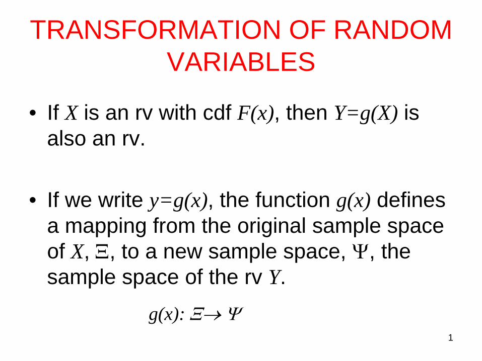
1

TRANSFORMATION OF RANDOM VARIABLES

• If X is an rv with cdf F(x), then Y=g(X) is also an rv.

• If we write y=g(x), the function g(x) defines a mapping from the original sample space of X, Ξ, to a new sample space, Ψ, the sample space of the rv Y.

g(x): Ξ→ Ψ

2

TRANSFORMATION OF RANDOM VARIABLES

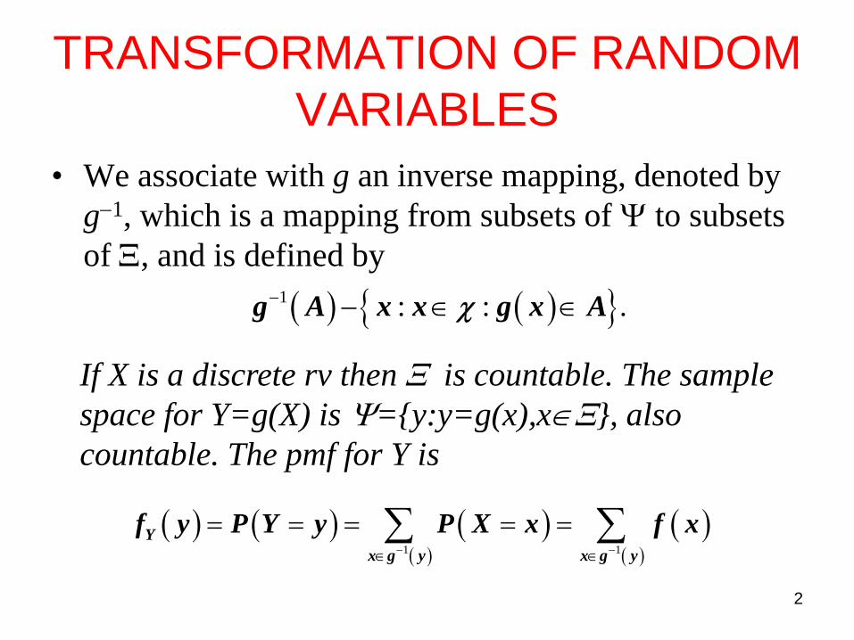
• We associate with g an inverse mapping, denoted by g−1, which is a mapping from subsets of Ψ to subsets of Ξ, and is defined by

( ) ( ){ }1 : : .g A x x g x Aχ− − ∈ ∈

If X is a discrete rv then Ξ is countable. The sample space for Y=g(X) is Ψ={y:y=g(x),x∈Ξ}, also countable. The pmf for Y is

( ) ( ) ( )( )

( )( )1 1

Yx g y x g y

f y P Y y P X x f x− −∈ ∈

= = = = =∑ ∑

3

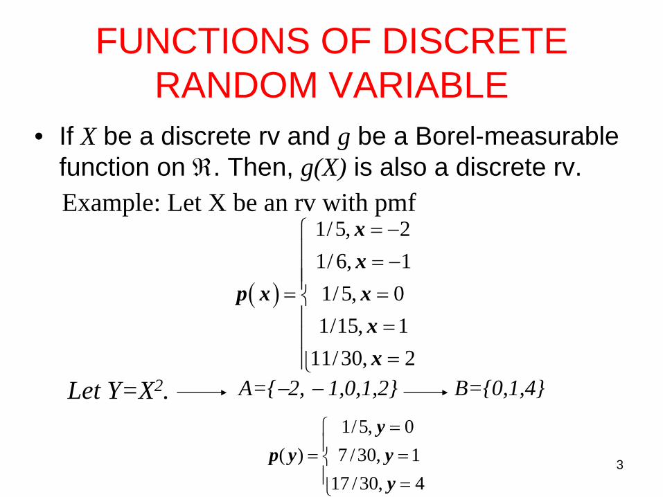
FUNCTIONS OF DISCRETE RANDOM VARIABLE

• If X be a discrete rv and g be a Borel-measurable function on ℜ. Then, g(X) is also a discrete rv.

( )

1/5, 21/ 6, 11/5, 01/15, 1

11/30, 2

xx

p x xxx

= −⎧⎪ = −⎪⎪= =⎨⎪ =⎪

=⎪⎩

Example: Let X be an rv with pmf

Let Y=X2. A={−2, − 1,0,1,2} B={0,1,4}

1/5, 0( ) 7 /30, 1

17 /30, 4

yp y y

y

=⎧⎪= =⎨⎪ =⎩

4

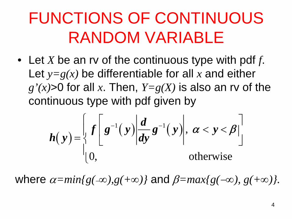
FUNCTIONS OF CONTINUOUS RANDOM VARIABLE

• Let X be an rv of the continuous type with pdf f. Let y=g(x) be differentiable for all x and either g’(x)>0 for all x. Then, Y=g(X) is also an rv of the continuous type with pdf given by

( ) ( ) ( )1 1 ,

0, otherwise

df g y g y yh y dy

α β− −⎧ ⎡ ⎤

< <⎪ ⎢ ⎥= ⎨ ⎣ ⎦⎪⎩

where α=min{g(−∞),g(+∞)} and β=max{g(−∞), g(+∞)}.

5

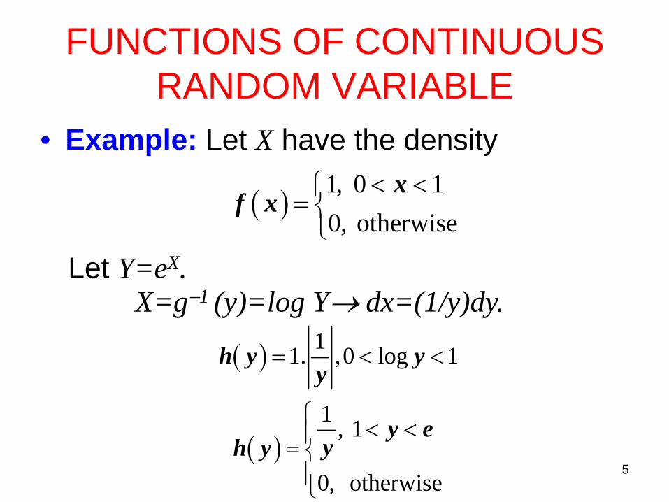
FUNCTIONS OF CONTINUOUS RANDOM VARIABLE

• Example: Let X have the density

( )1, 0 10, otherwise

xf x

< <⎧= ⎨⎩

Let Y=eX.X=g−1 (y)=log Y→ dx=(1/y)dy.

( )

( )

11. ,0 log 1

1 , 1

0, otherwise

h y yy

y eyh y

= < <

⎧ < <⎪= ⎨⎪⎩

6

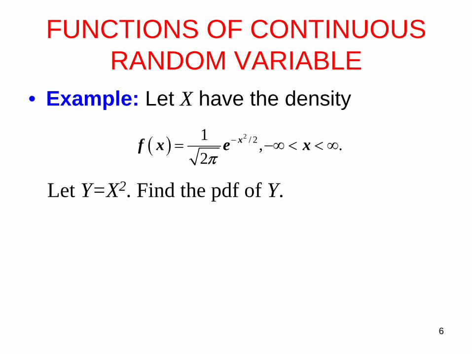
FUNCTIONS OF CONTINUOUS RANDOM VARIABLE

• Example: Let X have the density

( ) 2 / 21 , .2

xf x e xπ

−= −∞ < < ∞

Let Y=X2. Find the pdf of Y.

7

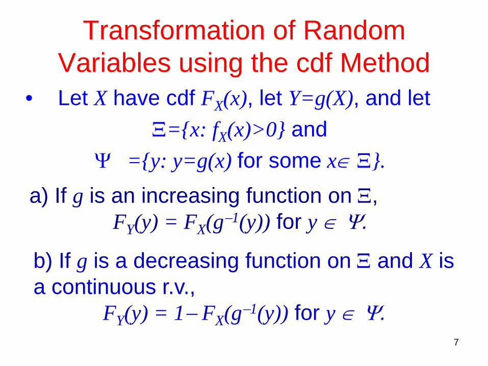
Transformation of Random Variables using the cdf Method

• Let X have cdf FX(x), let Y=g(X), and let Ξ={x: fX(x)>0} and

Ψ ={y: y=g(x) for some x∈ Ξ}.a) If g is an increasing function on Ξ,

FY(y) = FX(g−1(y)) for y ∈ Ψ.

b) If g is a decreasing function on Ξ and X is a continuous r.v.,

FY(y) = 1− FX(g−1(y)) for y ∈ Ψ.

8

EXAMPLE

• Suppose X ~ fX(x) = 1 if 0<x<1 and 0otherwise. Find the distribution function of Y=g(X)=− log X.

Uniform(0,1)distribution

9

THE PROBABILITY INTEGRAL TRANSFORMATION

• Let X have continuous cdf FX(x) and define the rv Y as Y=FX(x). Then, Y is uniformly distributed on (0,1), that is,

P(Y ≤ y) = y, 0<y<1.

10

Describing the Population or The Probability Distribution

• The probability distribution represents a population

• We’re interested in describing the population by computing various parameters.

• Specifically, we calculate the population mean and population variance.

11

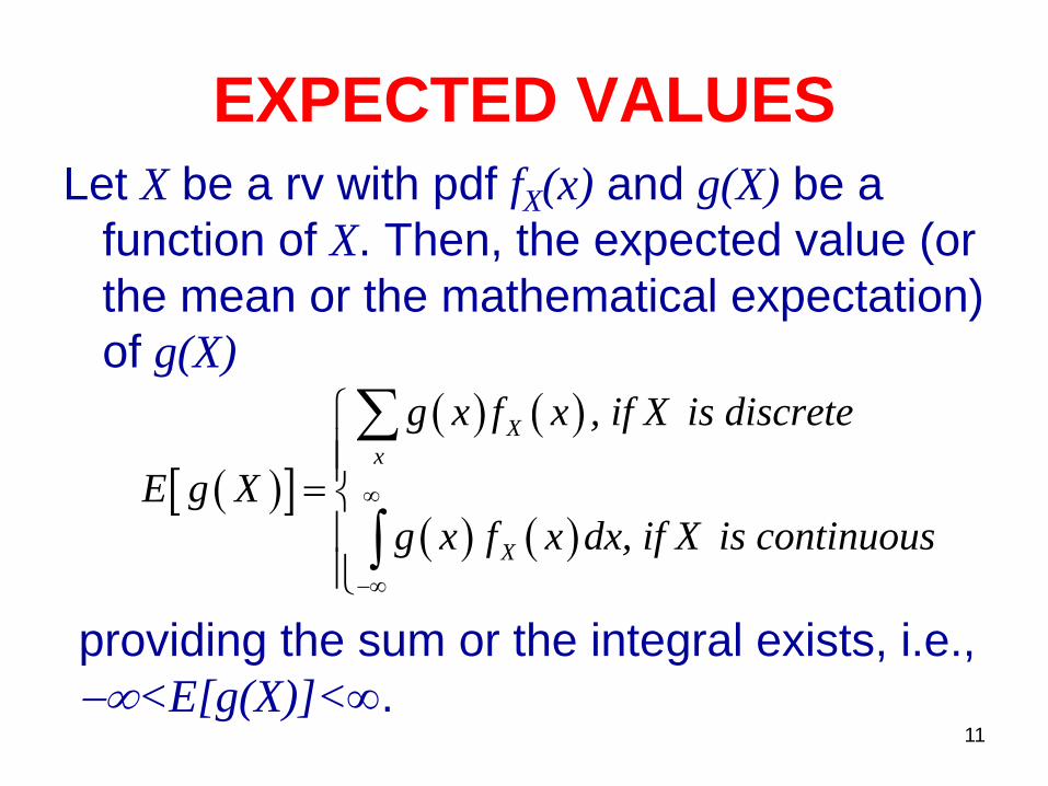
EXPECTED VALUESLet X be a rv with pdf fX(x) and g(X) be a

function of X. Then, the expected value (or the mean or the mathematical expectation) of g(X)

( )[ ]( ) ( )

( ) ( )

Xx

X

g x f x , if X is discrete

E g Xg x f x dx, if X is continuous

∞

−∞

⎧⎪⎪= ⎨⎪⎪⎩

∑

∫providing the sum or the integral exists, i.e.,−∞<E[g(X)]<∞.

12

EXPECTED VALUES

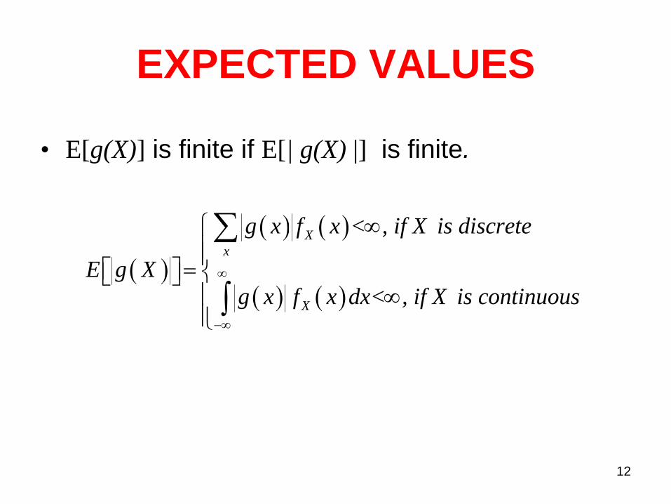
• E[g(X)] is finite if E[| g(X) |] is finite.

( )

( ) ( )

( ) ( )

Xx

X

g x f x < , if X is discrete

E g Xg x f x dx< , if X is continuous

∞

−∞

∞⎧⎪⎪=⎡ ⎤ ⎨⎣ ⎦⎪ ∞⎪⎩

∑

∫

13

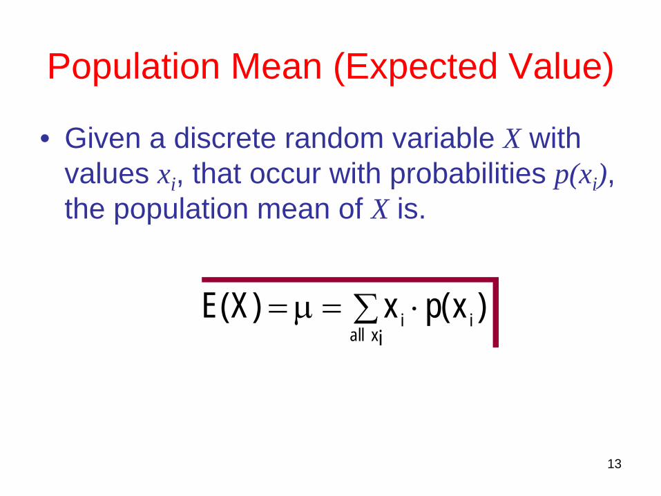
Population Mean (Expected Value)

• Given a discrete random variable X with values xi, that occur with probabilities p(xi), the population mean of X is.

∑ ⋅=μ=ixall

ii )x(px)X(E

14

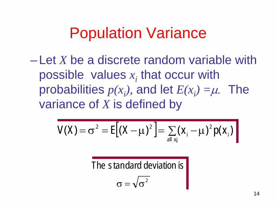
– Let X be a discrete random variable with possible values xi that occur with probabilities p(xi), and let E(xi) =μ. The variance of X is defined by

[ ] ∑ μ−=μ−=σ=ixall

i2

i22 )x(p)x()X(E)X(V

Population Variance

2

isdeviationdardtansThe

σ=σ

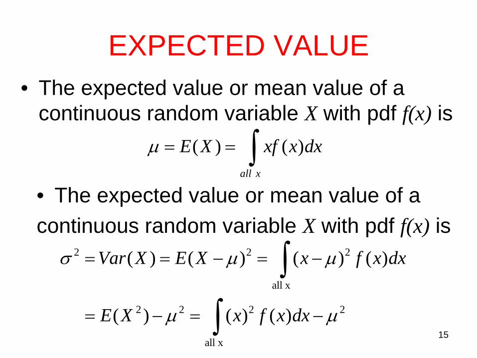
15

EXPECTED VALUE• The expected value or mean value of a

continuous random variable X with pdf f(x) is( ) ( )

all x

E X xf x dxμ = = ∫• The expected value or mean value of a continuous random variable X with pdf f(x) is

2 2 2

all x

2 2 2 2

all x

( ) ( ) ( ) ( )

( ) ( ) ( )

Var X E X x f x dx

E X x f x dx

σ μ μ

μ μ

= = − = −

= − = −

∫

∫

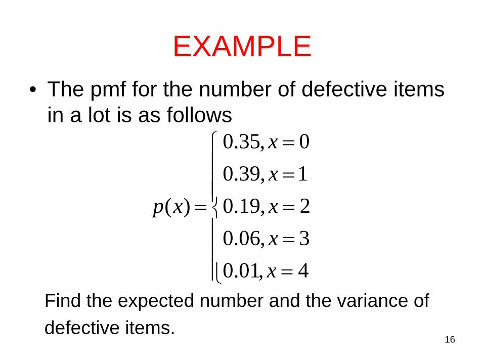
16

EXAMPLE• The pmf for the number of defective items

in a lot is as follows0.35, 00.39, 1

( ) 0.19, 20.06, 30.01, 4

xx

p x xxx

=⎧⎪ =⎪⎪= =⎨⎪ =⎪

=⎪⎩Find the expected number and the variance of defective items.

17

EXAMPLE

• What is the mathematical expectation if we win $10 when a die comes up 1 or 6 and lose $5 when it comes up 2, 3, 4 and 5?

X = amount of profit

18

EXAMPLE• A grab-bay contains 6 packages worth $2

each, 11 packages worth $3, and 8 packages worth $4 each. Is it reasonable to pay $3.5 for the option of selecting one of these packages at random?

X = worth of packages

19

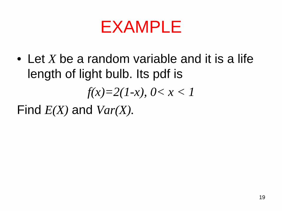
EXAMPLE

• Let X be a random variable and it is a life length of light bulb. Its pdf is

f(x)=2(1-x), 0< x < 1Find E(X) and Var(X).

20

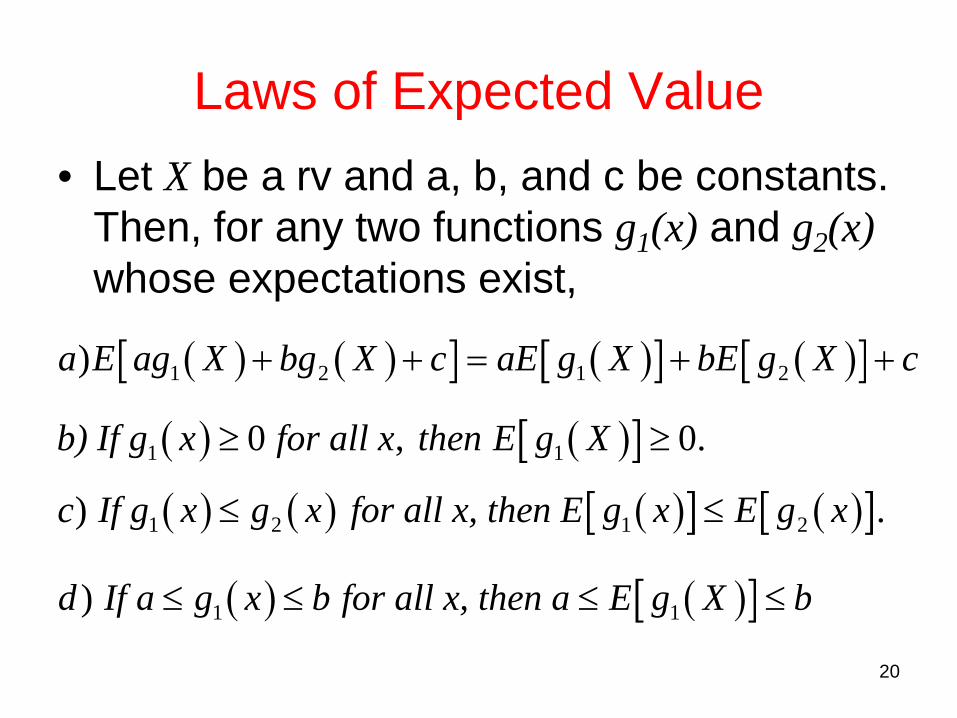
Laws of Expected Value• Let X be a rv and a, b, and c be constants.

Then, for any two functions g1(x) and g2(x)whose expectations exist,

( ) ( )[ ] ( )[ ] ( )[ ]1 2 1 2)a E ag X bg X c aE g X bE g X c+ + = + +

( ) ( )[ ]1 10 , 0.b) If g x for all x then E g X≥ ≥

( ) ( ) ( )[ ] ( )[ ]1 2 1 2) .c If g x g x for all x, then E g x E g x≤ ≤

( ) ( )[ ]1 1)d If a g x b for all x, then a E g X b ≤ ≤ ≤ ≤

21

Laws of Expected Value

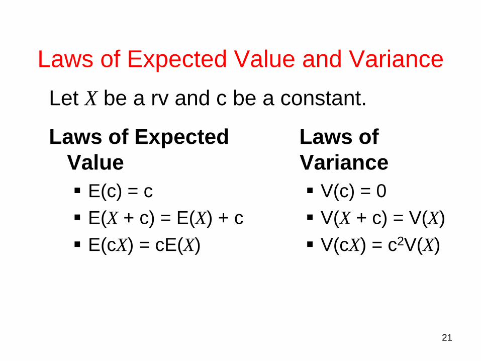
E(c) = cE(X + c) = E(X) + cE(cX) = cE(X)

Laws of Variance

V(c) = 0V(X + c) = V(X)V(cX) = c2V(X)

Laws of Expected Value and VarianceLet X be a rv and c be a constant.

22

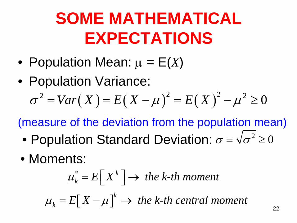
SOME MATHEMATICAL EXPECTATIONS

• Population Mean: μ = E(X)• Population Variance:

( ) ( ) ( )2 22 2 0Var X E X E Xσ μ μ= = − = − ≥

(measure of the deviation from the population mean)• Population Standard Deviation: 2 0σ σ= ≥

• Moments:* kk E X the k-th momentμ ⎡ ⎤= →⎣ ⎦

[ ]kk E X the k-th central momentμ μ= − →

23

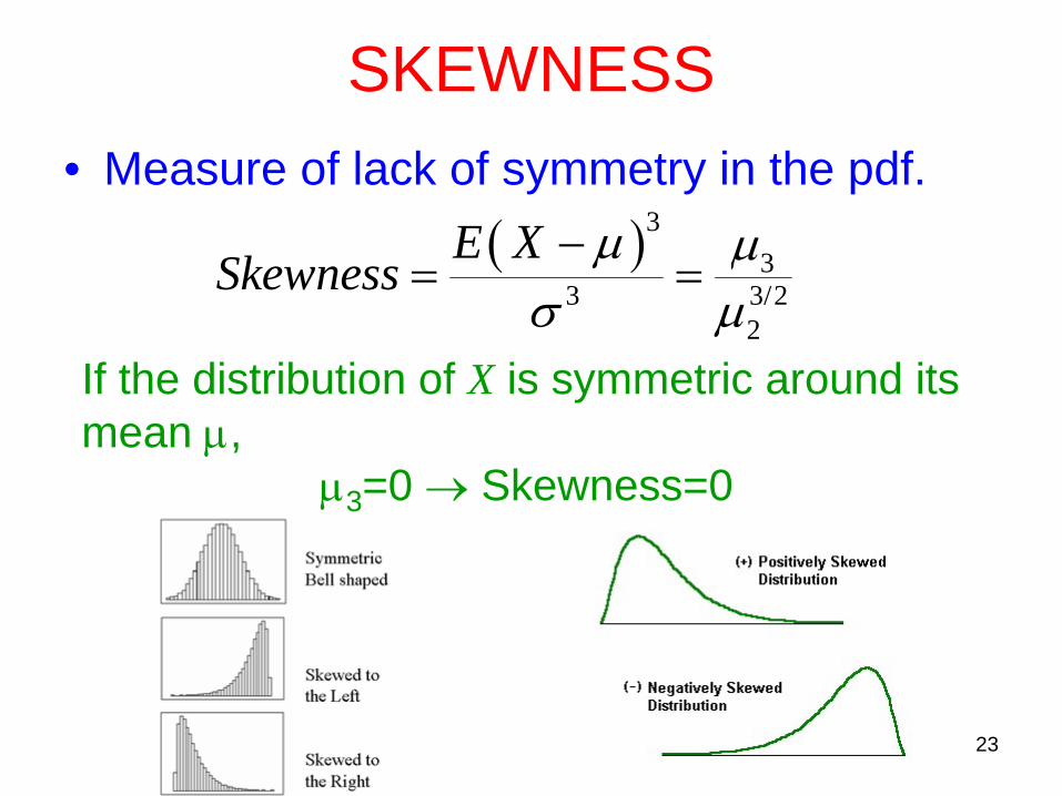
SKEWNESS• Measure of lack of symmetry in the pdf.

( )33

3 3/22

E XSkewness μ μσ μ−

= =

If the distribution of X is symmetric around its mean μ,

μ3=0 → Skewness=0

24

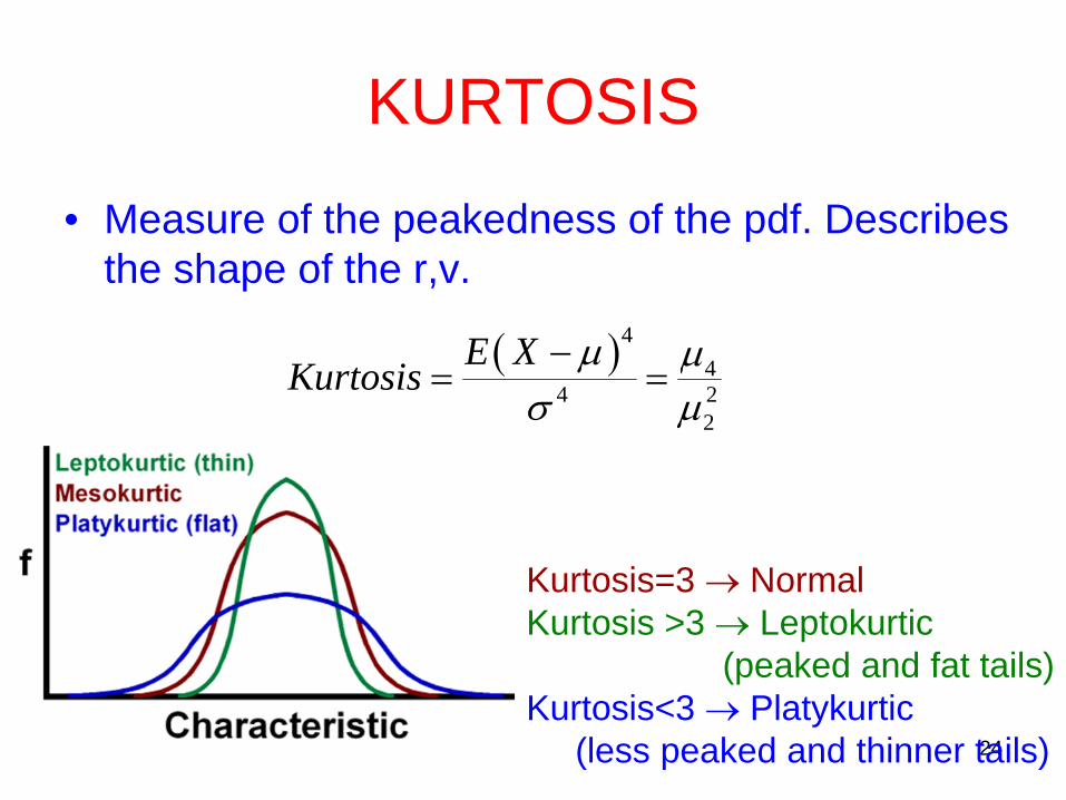
KURTOSIS

• Measure of the peakedness of the pdf. Describes the shape of the r,v.

( )44

4 22

E XKurtosis μ μσ μ−

= =

Kurtosis=3 → NormalKurtosis >3 → Leptokurtic

(peaked and fat tails)Kurtosis<3 → Platykurtic

(less peaked and thinner tails)

25

Measures of Central Location

• Usually, we focus our attention on two types of measures when describing population characteristics:– Central location– Variability or spread

The measure of central location reflects the locations of all the actual data points.

26

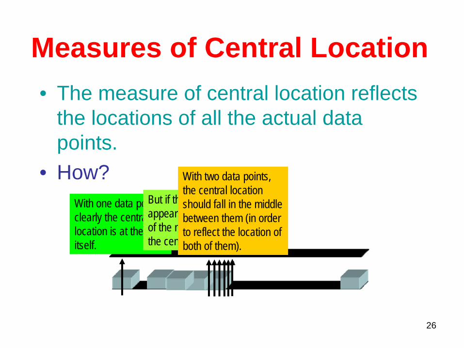
With one data pointclearly the central location is at the pointitself.

Measures of Central Location• The measure of central location reflects

the locations of all the actual data points.

• How?But if the third data point appears on the left hand-sideof the midrange, it should “pull”the central location to the left.

With two data points,the central location should fall in the middlebetween them (in order to reflect the location ofboth of them).

27

Sum of the observationsNumber of observationsMean =

• This is the most popular and useful measure of central location

The Arithmetic Mean

28

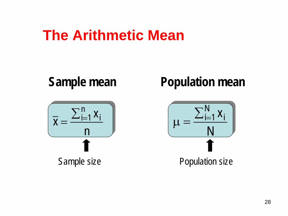
nxx i

n1i=∑

=

Sample mean Population mean

Nxi

N1i=∑

=μ

Sample size Population size

nxx i

n1i=∑

=

The Arithmetic Mean

29

=+++

=∑

= =

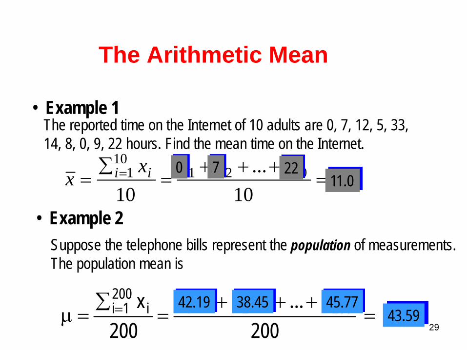
10...

101021

101 xxxx

x ii

• Example 1The reported time on the Internet of 10 adults are 0, 7, 12, 5, 33, 14, 8, 0, 9, 22 hours. Find the mean time on the Internet.

0 7 2211.0

• Example 2Suppose the telephone bills represent the population of measurements. The population mean is

=+++

=∑

=μ =

200x...xx

200x 20021i

2001i 42.19 38.45 45.77

43.59

The Arithmetic Mean

30

The Arithmetic Mean

• Drawback of the mean:It can be influenced by unusual

observations, because it uses all the information in the data set.

31

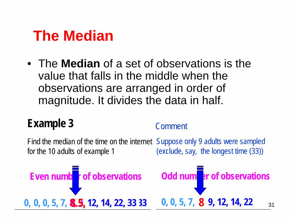
Odd number of observations

0, 0, 5, 7, 8 9, 12, 14, 220, 0, 5, 7, 8, 9, 12, 14, 22, 330, 0, 5, 7, 8, 9, 12, 14, 22, 33

Even number of observations

Example 3Find the median of the time on the internetfor the 10 adults of example 1

• The Median of a set of observations is the value that falls in the middle when the observations are arranged in order of magnitude. It divides the data in half.

The Median

Suppose only 9 adults were sampled (exclude, say, the longest time (33))

Comment

8.5, 8

32

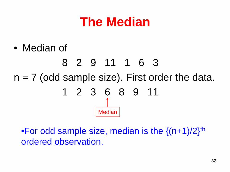
The Median

• Median of 8 2 9 11 1 6 3

n = 7 (odd sample size). First order the data.1 2 3 6 8 9 11

Median

•For odd sample size, median is the {(n+1)/2}th

ordered observation.

33

The Median• The engineering group receives e-mail

requests for technical information from sales and services person. The daily numbers for 6 days were

11, 9, 17, 19, 4, and 15.What is the central location of the data?

•For even sample sizes, the median is the average of {n/2}th and {n/2+1}th ordered observations.

34

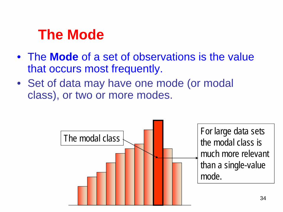
• The Mode of a set of observations is the value that occurs most frequently.

• Set of data may have one mode (or modal class), or two or more modes.

The modal classFor large data setsthe modal class is much more relevant than a single-value mode.

The Mode

35

• Find the mode for the data in Example 1. Here are the data again: 0, 7, 12, 5, 33, 14, 8, 0, 9, 22

Solution

• All observation except “0” occur once. There are two “0”. Thus, the mode is zero.

• Is this a good measure of central location?• The value “0” does not reside at the center of this set

(compare with the mean = 11.0 and the median = 8.5).

The Mode

36

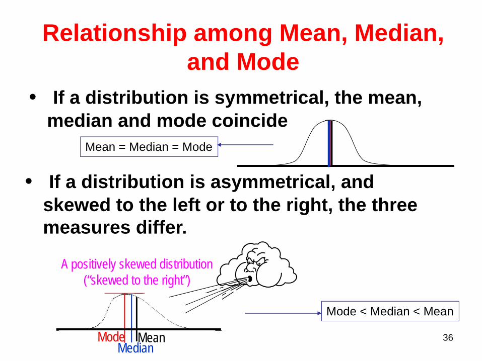
Relationship among Mean, Median, and Mode

• If a distribution is symmetrical, the mean, median and mode coincide

• If a distribution is asymmetrical, and skewed to the left or to the right, the three measures differ.

A positively skewed distribution(“skewed to the right”)

MeanMedian

Mode

Mean = Median = Mode

Mode < Median < Mean

37

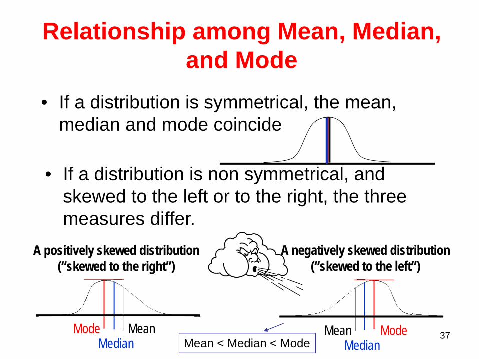
• If a distribution is symmetrical, the mean, median and mode coincide

• If a distribution is non symmetrical, and skewed to the left or to the right, the three measures differ.

A positively skewed distribution(“skewed to the right”)

MeanMedian

Mode MeanMedian

Mode

A negatively skewed distribution(“skewed to the left”)

Relationship among Mean, Median, and Mode

Mean < Median < Mode

38

MEAN, MEDIAN AND MODE

• Why are the mean, median, and mode like a valuable piece of real estate?

LOCATION! LOCATION! LOCATION!

• *All you beginning students of statistics just remember that measures of central tendancy are all POINTS on the score scale as oppposed to measures of variability which are all DISTANCES on the score scale. Understand this maxim and you will always know where you are LOCATED!

39

Measures of variability

• Measures of central location fail to tell the whole story about the distribution.

• A question of interest still remains unanswered:

How much are the observations spread outaround the mean value?

40

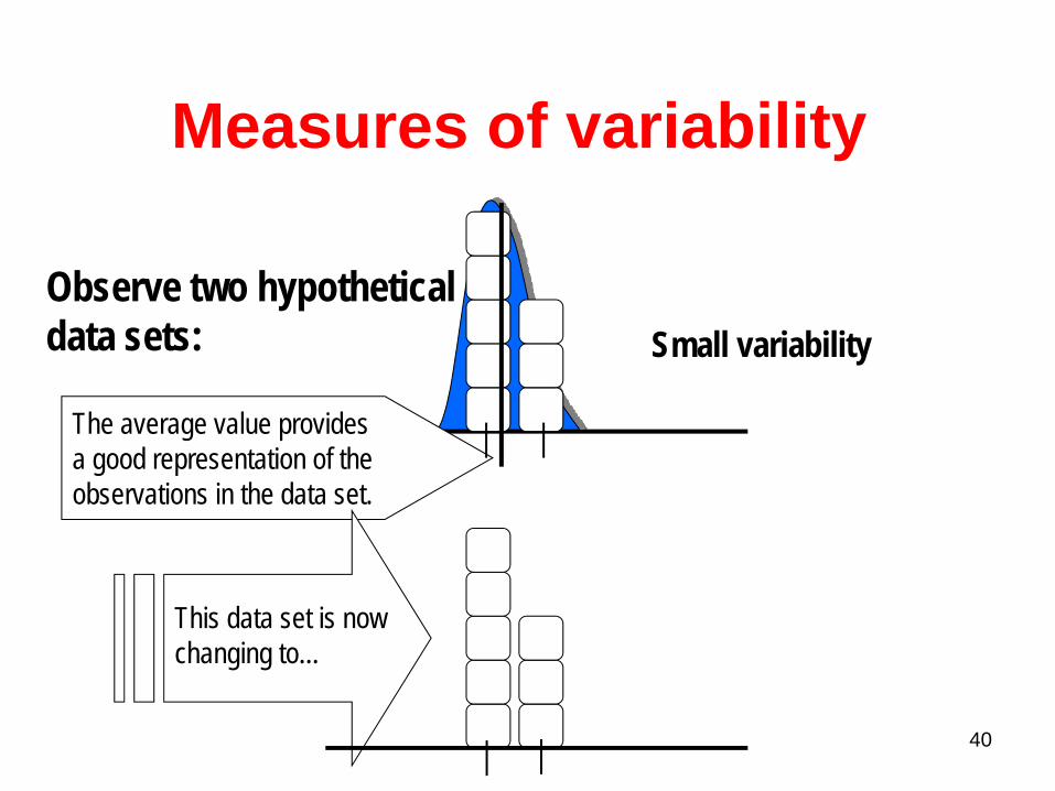
Measures of variability

Observe two hypothetical data sets:

The average value provides a good representation of theobservations in the data set.

Small variability

This data set is now changing to...

41

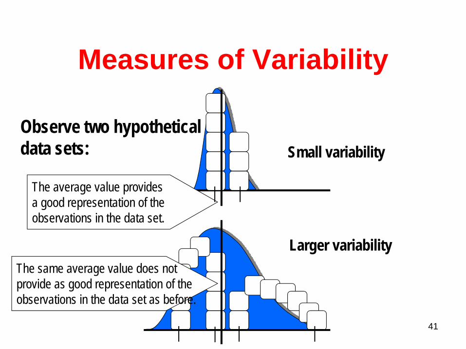
Measures of Variability

Observe two hypothetical data sets:

The average value provides a good representation of theobservations in the data set.

Small variability

Larger variabilityThe same average value does not provide as good representation of theobservations in the data set as before.

42

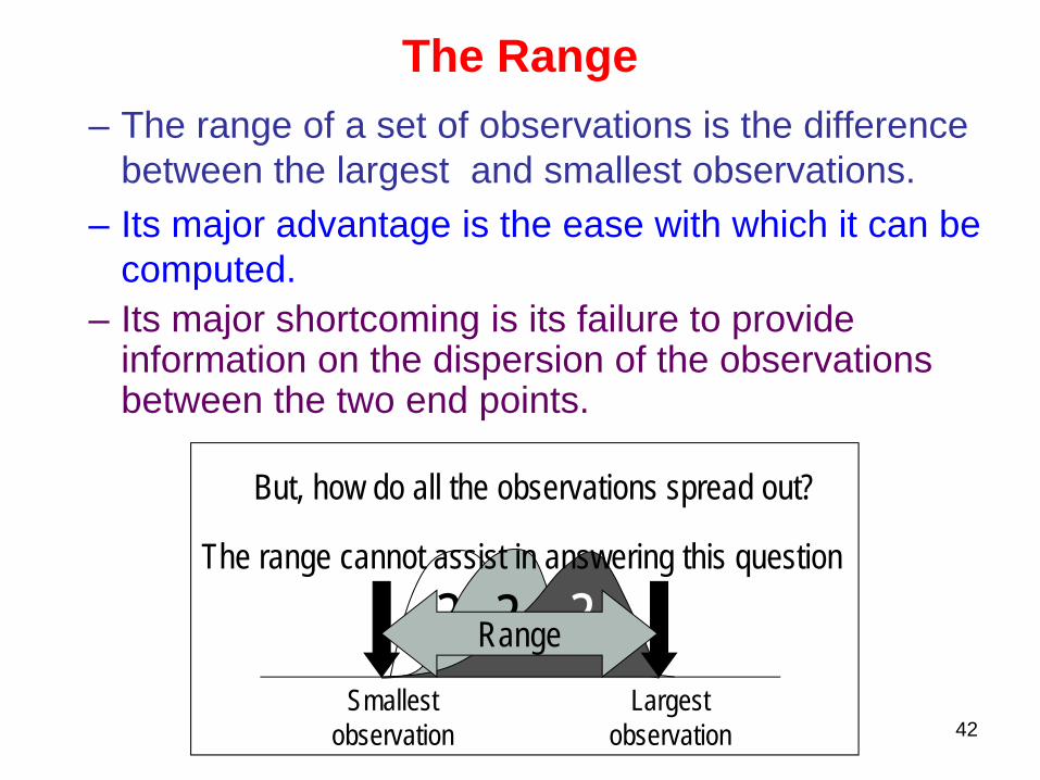
– The range of a set of observations is the difference between the largest and smallest observations.

– Its major advantage is the ease with which it can be computed.

– Its major shortcoming is its failure to provide information on the dispersion of the observations between the two end points.

? ? ?

But, how do all the observations spread out?

Smallestobservation

Largestobservation

The range cannot assist in answering this question

Range

The Range

43

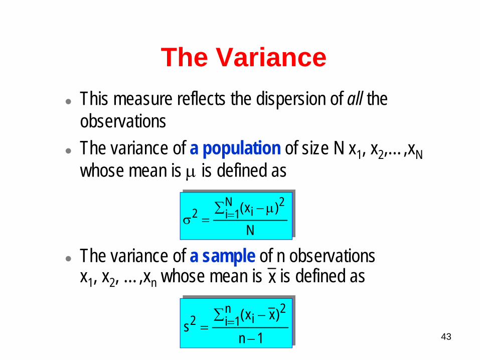
This measure reflects the dispersion of all the observationsThe variance of a population of size N x1, x2,…,xN whose mean is μ is defined as

The variance of a sample of n observationsx1, x2, …,xn whose mean is is defined asx

N)x( 2

iN

1i2 μ−∑=σ =

1n)xx(

s2

in

1i2−

−∑= =

The Variance

44

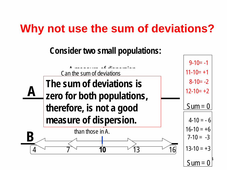
Why not use the sum of deviations?

Consider two small populations:

1098

74 10

11 12

13 16

8-10= -2

9-10= -111-10= +1

12-10= +2

4-10 = - 6

7-10 = -3

13-10 = +3

16-10 = +6

Sum = 0

Sum = 0

The mean of both populations is 10...

…but measurements in Bare more dispersedthan those in A.

A measure of dispersion Should agrees with this observation.

Can the sum of deviationsBe a good measure of dispersion?

A

B

The sum of deviations is zero for both populations, therefore, is not a good measure of dispersion.

45

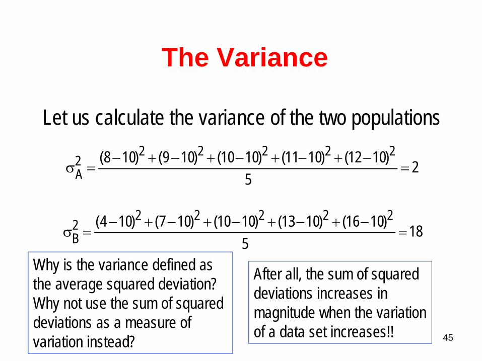
Let us calculate the variance of the two populations

185

)1016()1013()1010()107()104( 222222B =

−+−+−+−+−=σ

25

)1012()1011()1010()109()108( 222222A =

−+−+−+−+−=σ

Why is the variance defined as the average squared deviation?Why not use the sum of squared deviations as a measure of variation instead?

After all, the sum of squared deviations increases in magnitude when the variationof a data set increases!!

The Variance

46

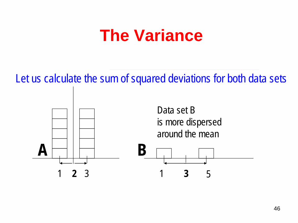
Which data set has a larger dispersion?

1 3 1 32 5

A B

Data set Bis more dispersedaround the mean

Let us calculate the sum of squared deviations for both data sets

The Variance

47

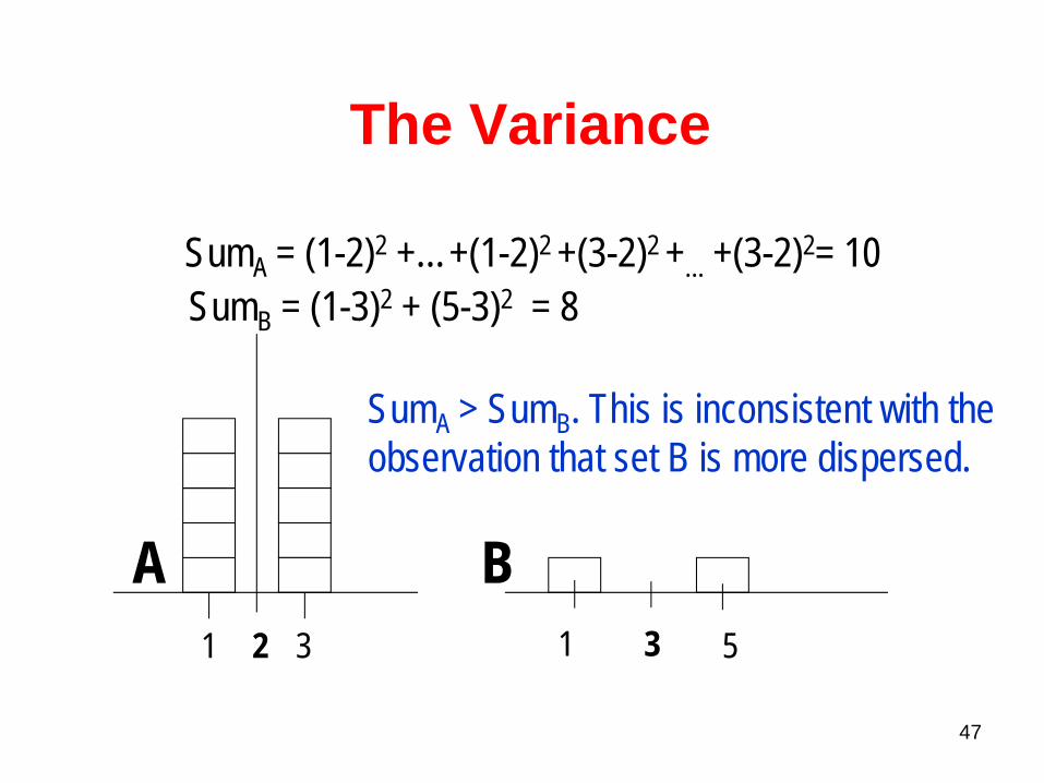
1 3 1 32 5

A B

SumA = (1-2)2 +…+(1-2)2 +(3-2)2 +… +(3-2)2= 10SumB = (1-3)2 + (5-3)2 = 8

SumA > SumB. This is inconsistent with the observation that set B is more dispersed.

The Variance

48

1 3 1 32 5

A B

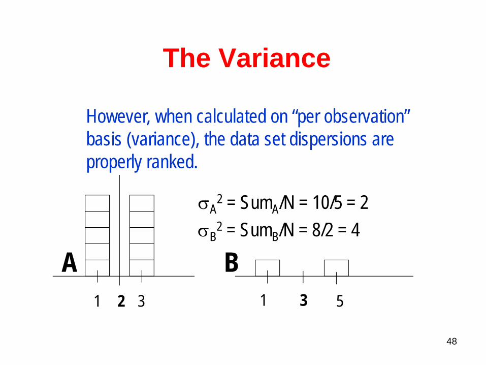
However, when calculated on “per observation” basis (variance), the data set dispersions are properly ranked.

σA2 = SumA/N = 10/5 = 2

σB2 = SumB/N = 8/2 = 4

The Variance

49

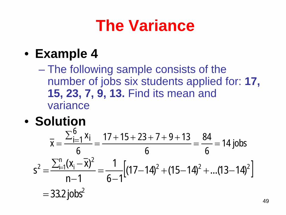
• Example 4– The following sample consists of the

number of jobs six students applied for: 17, 15, 23, 7, 9, 13. Find its mean and variance

• Solution

[ ]2

2222

in

1i2

jobs2.33

)1413...()1415()1417(16

11n

)xx(s

=

−+−+−−

=−−∑

= =

jobs146

846

13972315176

xx i

61i ==

+++++=

∑= =

The Variance

50

( ) ( )

2

2222

2i

n1i2

i

n

1i

2

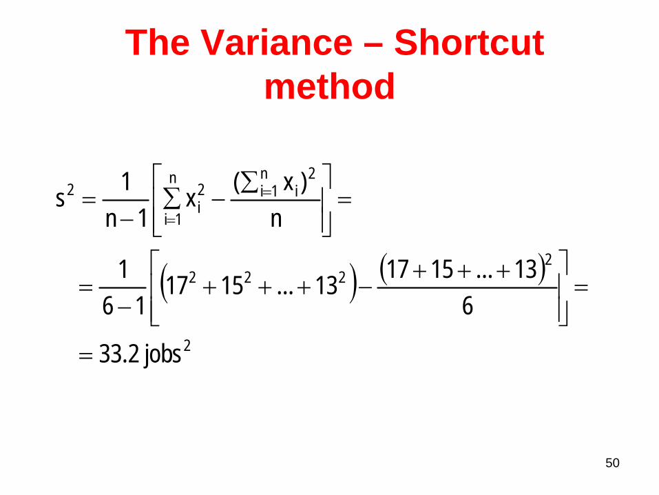
jobs2.33

613...151713...1517

161

n)x(x

1n1s

=

=⎥⎥⎦

⎤

⎢⎢⎣

⎡ +++−+++

−=

=⎥⎥⎦

⎤

⎢⎢⎣

⎡ ∑−∑

−= =

=

The Variance – Shortcut method

51

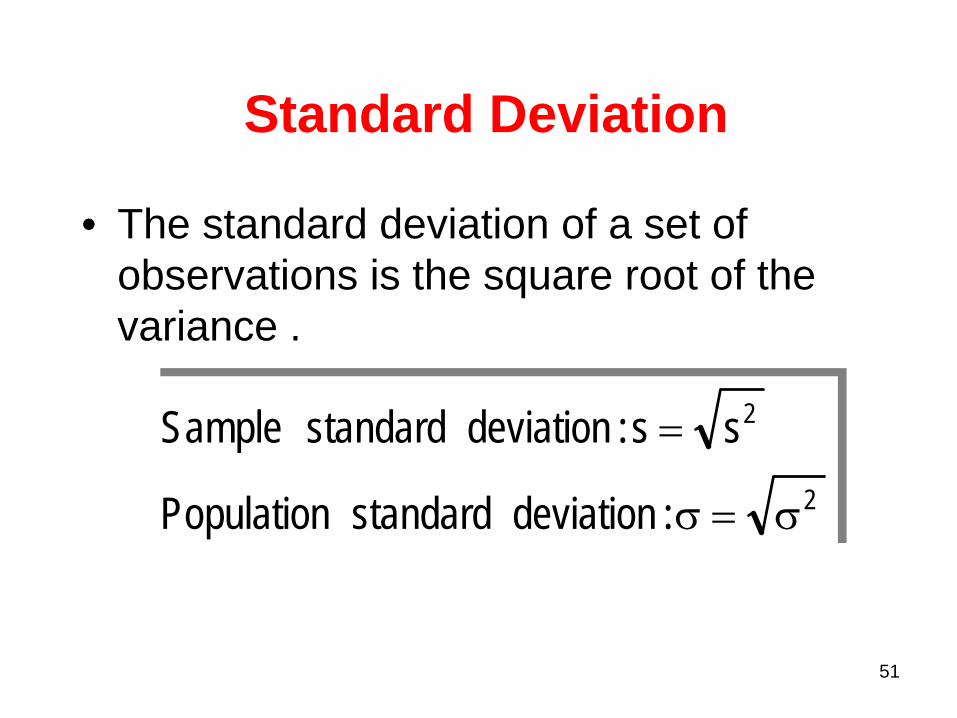
• The standard deviation of a set of observations is the square root of the variance .

2

2

:deviationandardstPopulation

ss:deviationstandardSample

σ=σ

=

Standard Deviation

52

• Example 5– To examine the consistency of shots for a

new innovative golf club, a golfer was asked to hit 150 shots, 75 with a currently used (7-iron) club, and 75 with the new club.

– The distances were recorded. – Which 7-iron is more consistent?

Standard Deviation

53

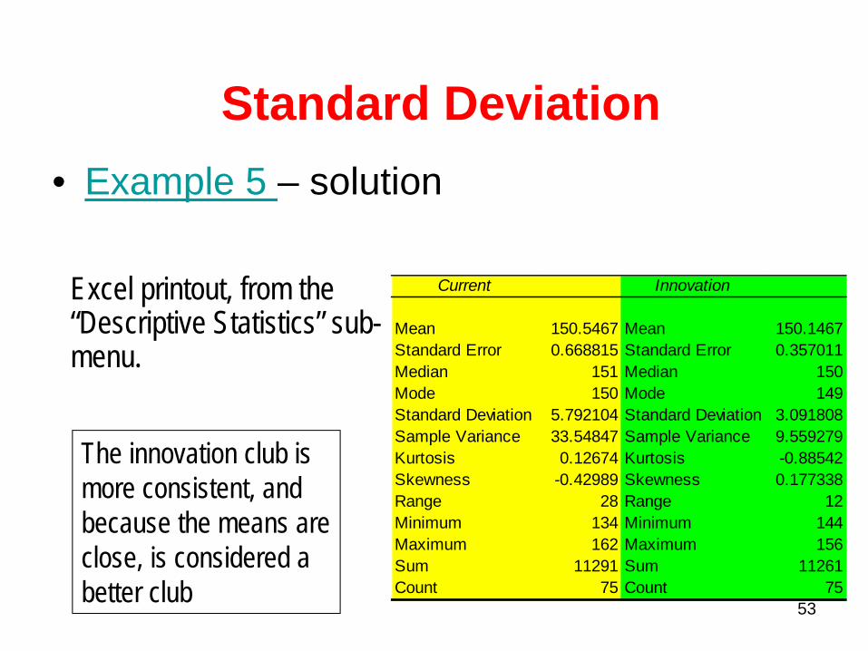
• Example 5 – solution

Standard Deviation

Excel printout, from the “Descriptive Statistics” sub-menu.

Current Innovation

Mean 150.5467 Mean 150.1467Standard Error 0.668815 Standard Error 0.357011Median 151 Median 150Mode 150 Mode 149Standard Deviation 5.792104 Standard Deviation 3.091808Sample Variance 33.54847 Sample Variance 9.559279Kurtosis 0.12674 Kurtosis -0.88542Skewness -0.42989 Skewness 0.177338Range 28 Range 12Minimum 134 Minimum 144Maximum 162 Maximum 156Sum 11291 Sum 11261Count 75 Count 75

The innovation club is more consistent, and because the means are close, is considered a better club

54

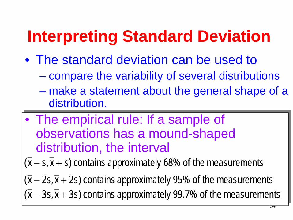
Interpreting Standard Deviation• The standard deviation can be used to

– compare the variability of several distributions– make a statement about the general shape of a

distribution. • The empirical rule: If a sample of

observations has a mound-shaped distribution, the interval

tsmeasuremen the of 68%ely approximat contains )sx,sx( +−

tsmeasuremen the of 95%ely approximat contains )s2x,s2x( +−tsmeasuremen the of 99.7%ely approximat contains )s3x,s3x( +−

55

• Example 6A statistics practitioner wants to describe the way returns on investment are distributed. – The mean return = 10%– The standard deviation of the return = 8%– The histogram is bell shaped.

Interpreting Standard Deviation

56

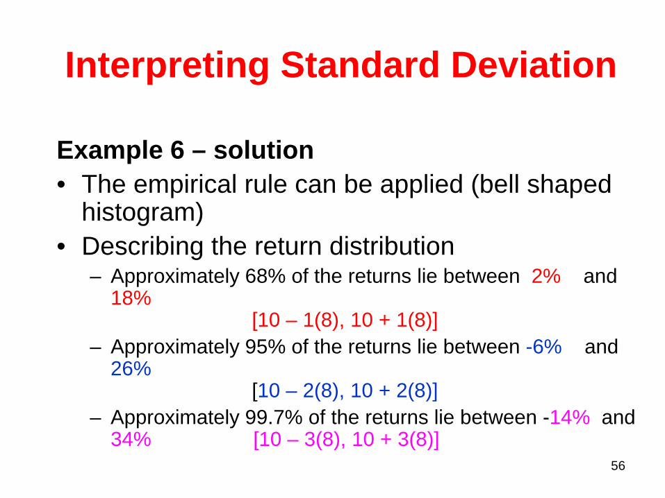
Example 6 – solution• The empirical rule can be applied (bell shaped

histogram)• Describing the return distribution

– Approximately 68% of the returns lie between 2% and 18%

[10 – 1(8), 10 + 1(8)]– Approximately 95% of the returns lie between -6% and

26%[10 – 2(8), 10 + 2(8)]

– Approximately 99.7% of the returns lie between -14% and 34% [10 – 3(8), 10 + 3(8)]

Interpreting Standard Deviation

57

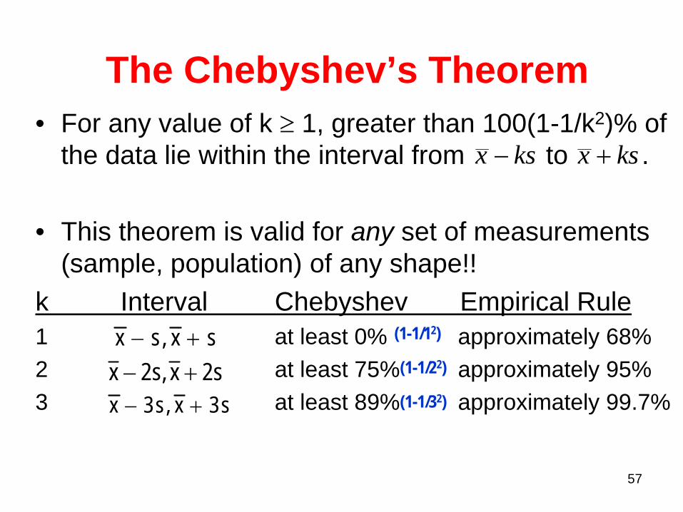
• For any value of k ≥ 1, greater than 100(1-1/k2)% of the data lie within the interval from to .

• This theorem is valid for any set of measurements (sample, population) of any shape!!

k Interval Chebyshev Empirical Rule1 at least 0% approximately 68%2 at least 75% approximately 95%3 at least 89% approximately 99.7%

s2x,s2x +−sx,sx +−

s3x,s3x +−

The Chebyshev’s Theorem

(1-1/12)

(1-1/22)

(1-1/32)

x ks− x ks+

58

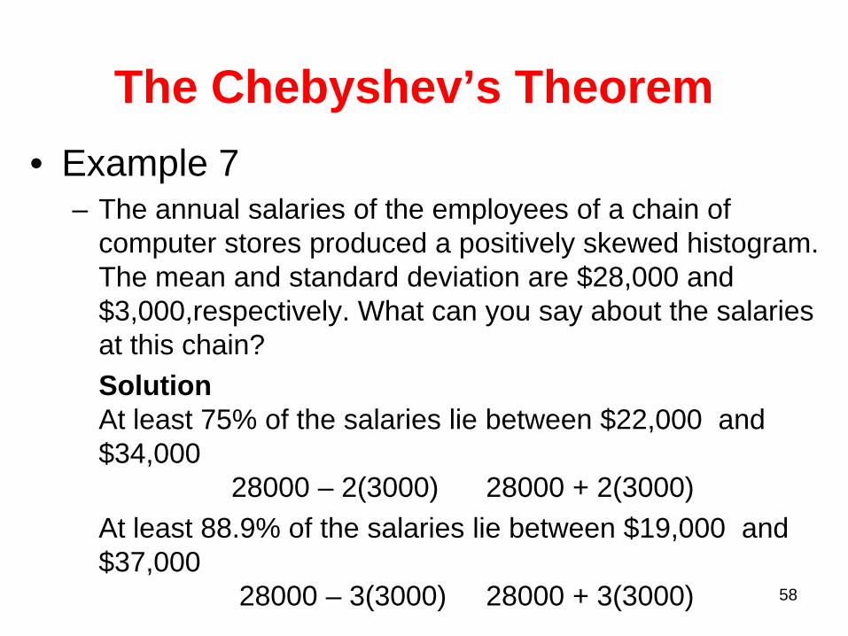
• Example 7– The annual salaries of the employees of a chain of

computer stores produced a positively skewed histogram. The mean and standard deviation are $28,000 and $3,000,respectively. What can you say about the salaries at this chain?SolutionAt least 75% of the salaries lie between $22,000 and $34,000

28000 – 2(3000) 28000 + 2(3000)At least 88.9% of the salaries lie between $19,000 and $37,000

28000 – 3(3000) 28000 + 3(3000)

The Chebyshev’s Theorem

59

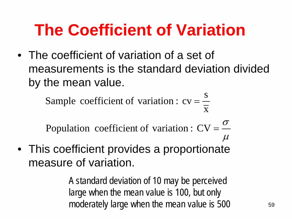
• The coefficient of variation of a set of measurements is the standard deviation divided by the mean value.

• This coefficient provides a proportionate measure of variation.

μσ

=

=

CV : variationoft coefficien Population

xscv : variationoft coefficien Sample

A standard deviation of 10 may be perceivedlarge when the mean value is 100, but only moderately large when the mean value is 500

The Coefficient of Variation

60Your score

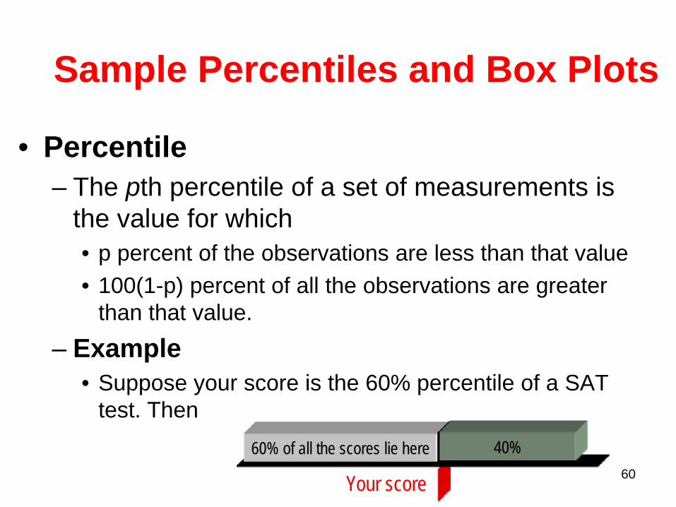
Sample Percentiles and Box Plots

• Percentile– The pth percentile of a set of measurements is

the value for which • p percent of the observations are less than that value• 100(1-p) percent of all the observations are greater

than that value.– Example

• Suppose your score is the 60% percentile of a SAT test. Then

60% of all the scores lie here 40%

61

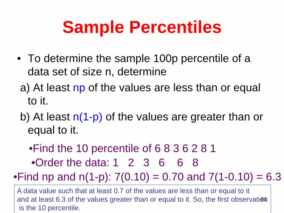
Sample Percentiles• To determine the sample 100p percentile of a

data set of size n, determinea) At least np of the values are less than or equal

to it.b) At least n(1-p) of the values are greater than or

equal to it. •Find the 10 percentile of 6 8 3 6 2 8 1•Order the data: 1 2 3 6 6 8

•Find np and n(1-p): 7(0.10) = 0.70 and 7(1-0.10) = 6.3A data value such that at least 0.7 of the values are less than or equal to it and at least 6.3 of the values greater than or equal to it. So, the first observationis the 10 percentile.

62

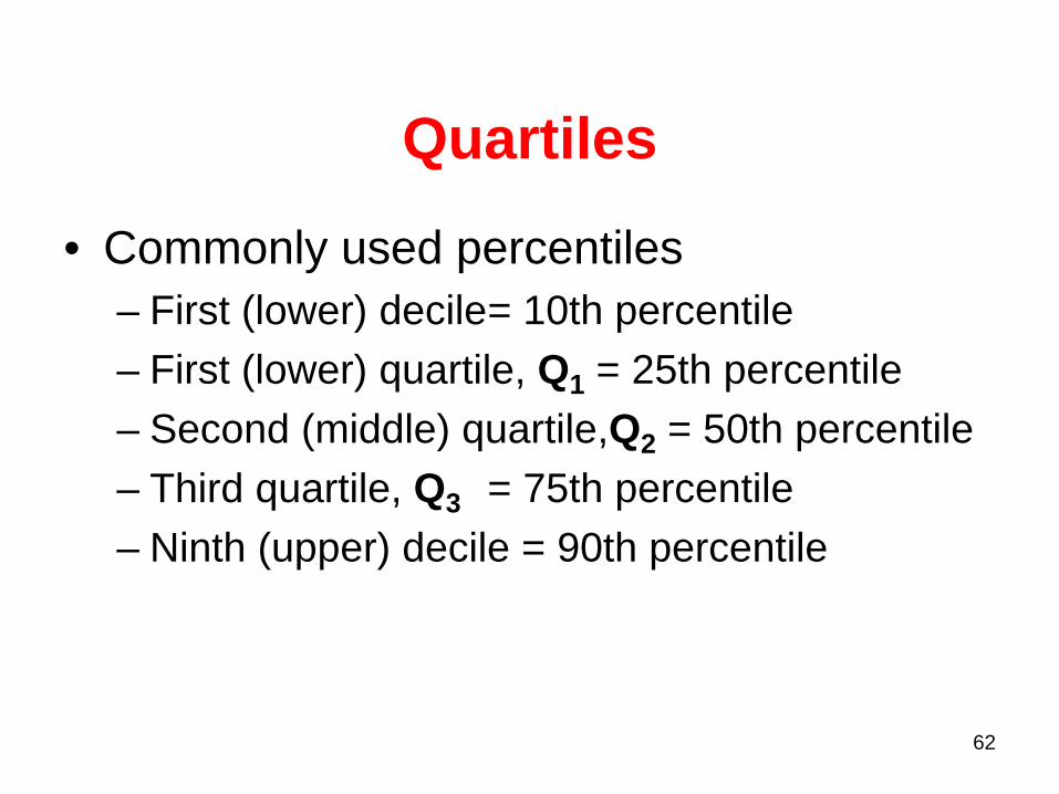
• Commonly used percentiles– First (lower) decile= 10th percentile– First (lower) quartile, Q1 = 25th percentile– Second (middle) quartile,Q2 = 50th percentile– Third quartile, Q3 = 75th percentile– Ninth (upper) decile = 90th percentile

Quartiles

63

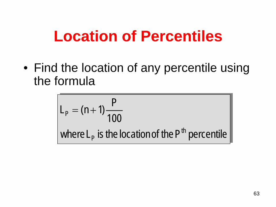
• Find the location of any percentile using the formula

Location of Percentiles

percentilePtheoflocationtheisLwhere100P)1n(L

thP

P +=

64

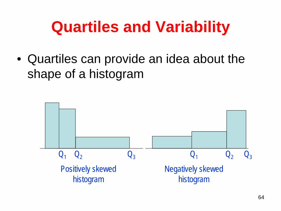
Quartiles and Variability

• Quartiles can provide an idea about the shape of a histogram

Q1 Q2 Q3

Positively skewedhistogram

Q1 Q2 Q3

Negatively skewedhistogram

65

• This is a measure of the spread of the middle 50% of the observations

• Large value indicates a large spread of the observations

Interquartile range = Q3 – Q1

Interquartile Range

66

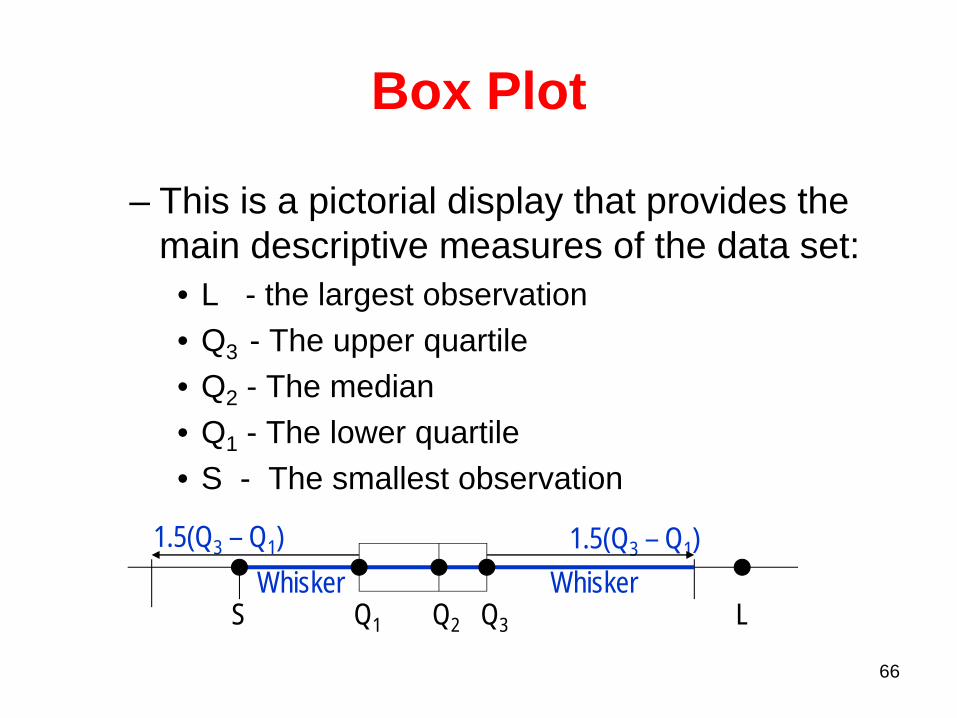
1.5(Q3 – Q1) 1.5(Q3 – Q1)

– This is a pictorial display that provides the main descriptive measures of the data set:

• L - the largest observation• Q3 - The upper quartile • Q2 - The median• Q1 - The lower quartile• S - The smallest observation

S Q1 Q2 Q3 LWhisker Whisker

Box Plot

67

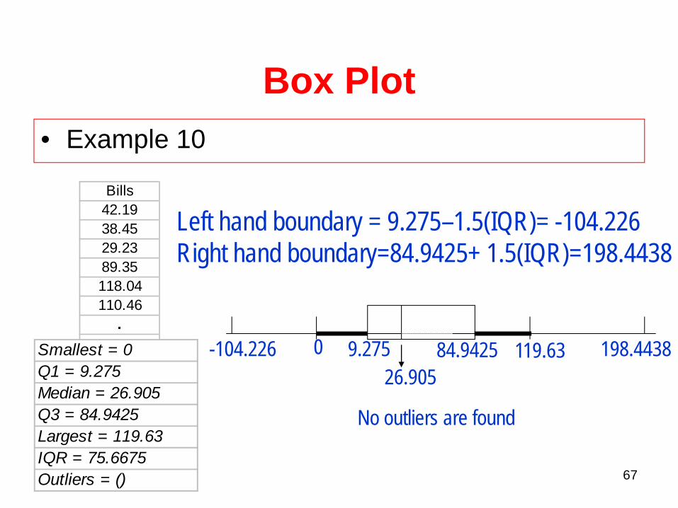
• Example 10

Box Plot

Bills42.1938.4529.2389.35118.04110.46

.

.

.Smallest = 0Q1 = 9.275Median = 26.905Q3 = 84.9425Largest = 119.63IQR = 75.6675Outliers = ()

Left hand boundary = 9.275–1.5(IQR)= -104.226Right hand boundary=84.9425+ 1.5(IQR)=198.4438

9.2750 84.9425 198.4438119.63-104.22626.905

No outliers are found

68

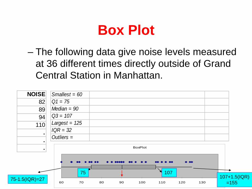
Box Plot– The following data give noise levels measured

at 36 different times directly outside of Grand Central Station in Manhattan.

NOISE828994

110...

Smallest = 60Q1 = 75Median = 90Q3 = 107Largest = 125IQR = 32Outliers =

BoxPlot

60 70 80 90 100 110 120 130

1077575-1.5(IQR)=27 107+1.5(IQR)

=155

69

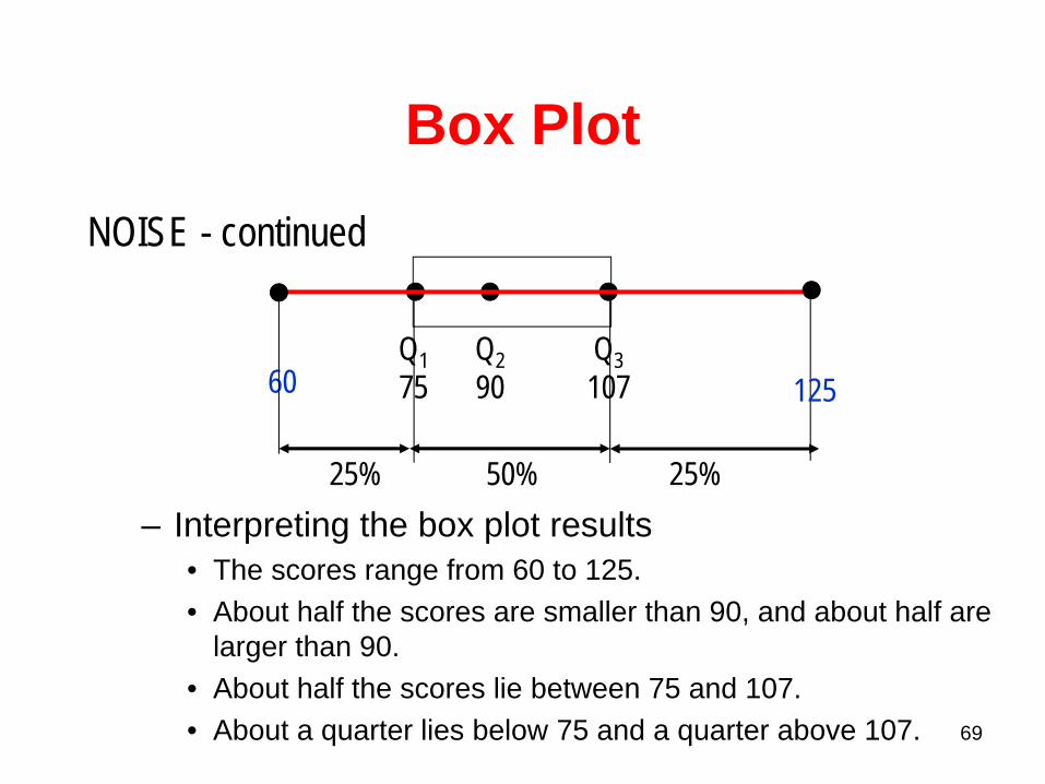
– Interpreting the box plot results• The scores range from 60 to 125.• About half the scores are smaller than 90, and about half are

larger than 90.• About half the scores lie between 75 and 107.• About a quarter lies below 75 and a quarter above 107.

Q175

Q290

Q3107

25% 50% 25%

60 125

Box Plot

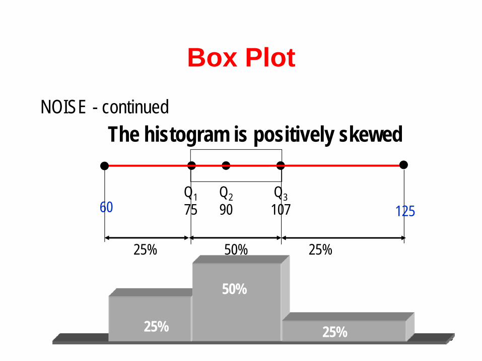
NOISE - continued

70

50%

25% 25%

The histogram is positively skewed

Q175

Q290

Q3107

25% 50% 25%

60 125

Box Plot

NOISE - continued

71

• Example 11– A study was organized to compare the quality of

service in 5 drive through restaurants.– Interpret the results

• Example 11 – solution– Minitab box plot (MINITAB 15 demo:

http://www.minitab.com/en-US/products/minitab/free-trial.aspx?langType=1033)

– To download SPSS18, follow the linkhttp://bidb.odtu.edu.tr/ccmscontent/articleRead/articleId/

articleRead/articleId/390

Box Plot

72

100 200 300

1

2

3

4

5

C6

C7

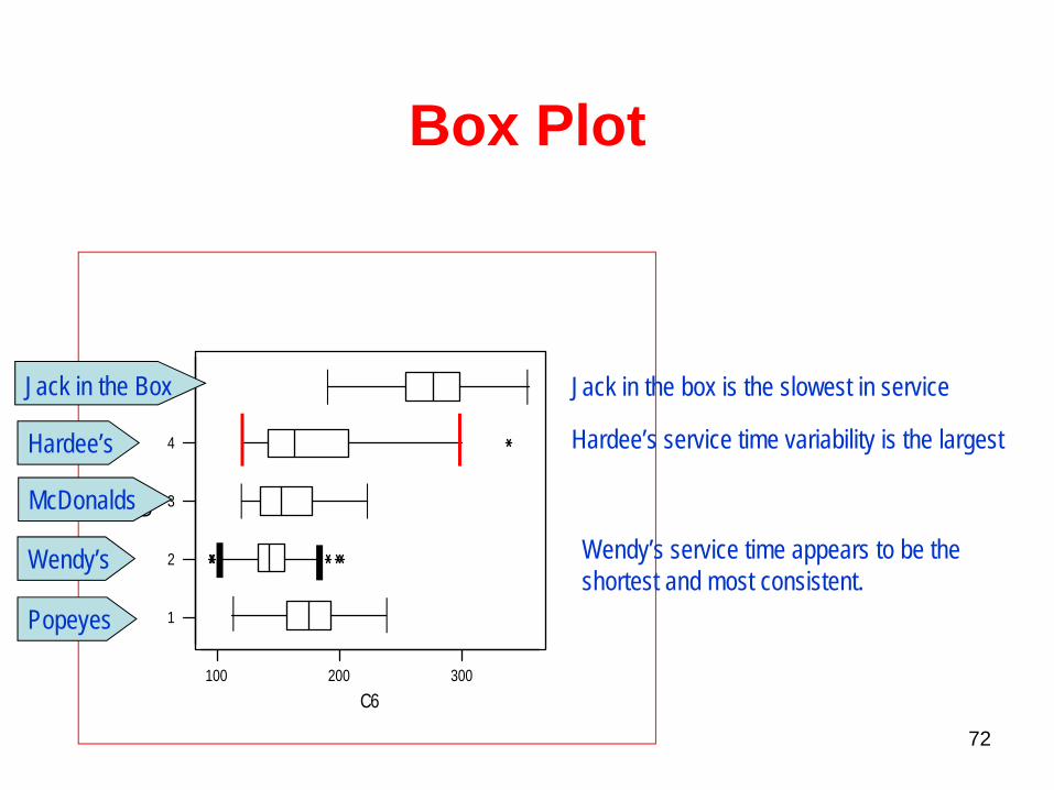
Wendy’s service time appears to be the shortest and most consistent.

Hardee’s service time variability is the largest

Jack in the box is the slowest in service

Box Plot

Jack in the Box

Hardee’s

McDonalds

Wendy’s

Popeyes

73

100 200 300

1

2

3

4

5

C6

C7

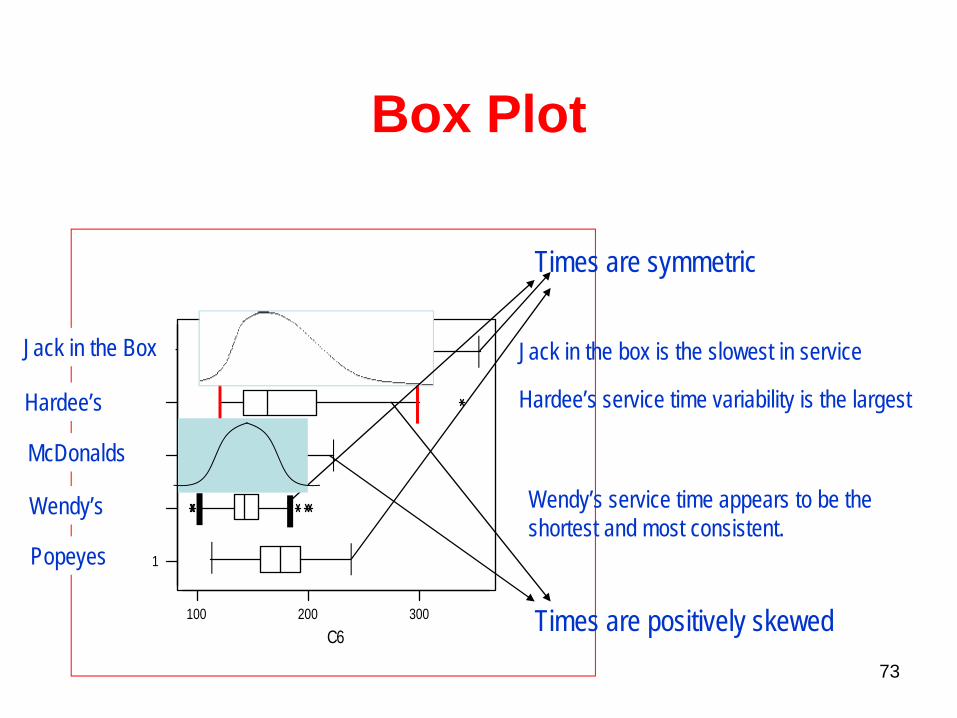
Popeyes

Wendy’s

Hardee’s

Jack in the Box

Wendy’s service time appears to be the shortest and most consistent.

McDonalds

Hardee’s service time variability is the largest

Jack in the box is the slowest in service

Box Plot

Times are positively skewed

Times are symmetric

74

Paired Data Sets and the Sample Correlation Coefficient

• The covariance and the coefficient of correlation are used to measure the direction and strength of the linear relationship between two variables.– Covariance - is there any pattern to the way

two variables move together? – Coefficient of correlation - how strong is the

linear relationship between two variables

75

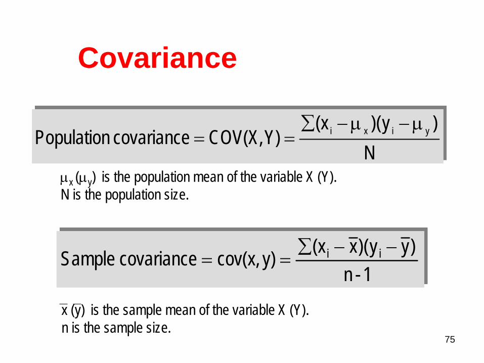
N)y)((x

Y)COV(X,covariance Population yixi μ−μ−∑==

μx (μy) is the population mean of the variable X (Y).N is the population size.

1-n)yy)(x(xy) cov(x,covariance Sample ii −−∑

==

Covariance

x (y) is the sample mean of the variable X (Y).n is the sample size.

76

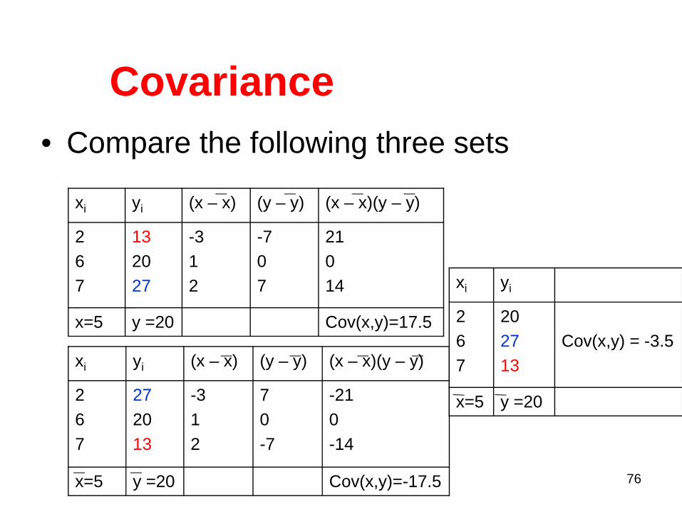
• Compare the following three sets

Covariance

xi yi (x – x) (y – y) (x – x)(y – y)

267

132027

-312

-707

21014

x=5 y =20 Cov(x,y)=17.5

xi yi (x – x) (y – y) (x – x)(y – y)

267

272013

-312

70-7

-210-14

x=5 y =20 Cov(x,y)=-17.5

xi yi

267

202713

Cov(x,y) = -3.5

x=5 y =20

77

• If the two variables move in opposite directions, (one increases when the other one decreases), the covariance is a large negative number.

• If the two variables are unrelated, the covariance will be close to zero.

• If the two variables move in the same direction, (both increase or both decrease), the covariance is a large positive number.

Covariance

78

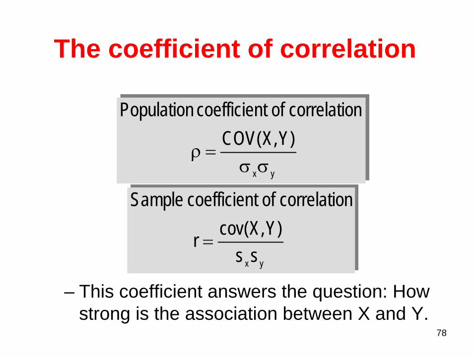
– This coefficient answers the question: How strong is the association between X and Y.

yx

)Y,X(COV

ncorrelatio oft coefficien Population

σσ=ρ

yx ss)Y,Xcov(r

ncorrelatio oft coefficien Sample

=

The coefficient of correlation

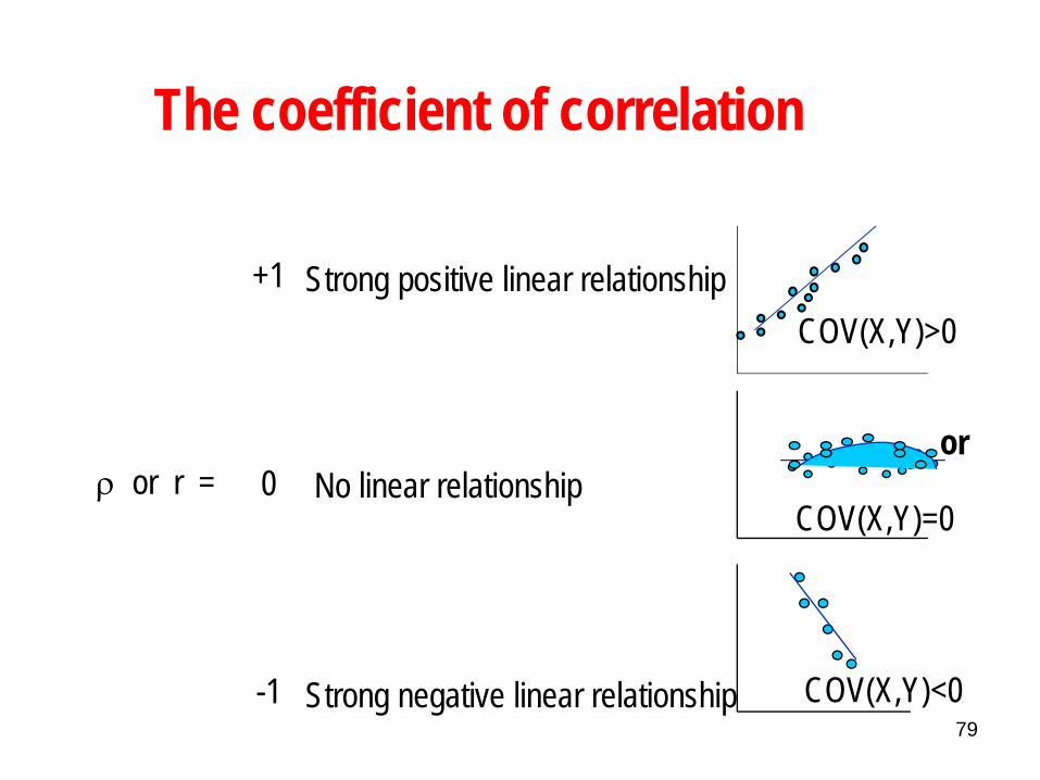
79

COV(X,Y)=0ρ or r =

+1

0

-1

Strong positive linear relationship

No linear relationship

Strong negative linear relationship

or

COV(X,Y)>0

COV(X,Y)<0

The coefficient of correlation

80

• If the two variables are very strongly positively related, the coefficient value is close to +1 (strong positive linear relationship).

• If the two variables are very strongly negatively related, the coefficient value is close to -1 (strong negative linear relationship).

• No straight line relationship is indicated by a coefficient close to zero.

The Coefficient of Correlation