12/8/16

1

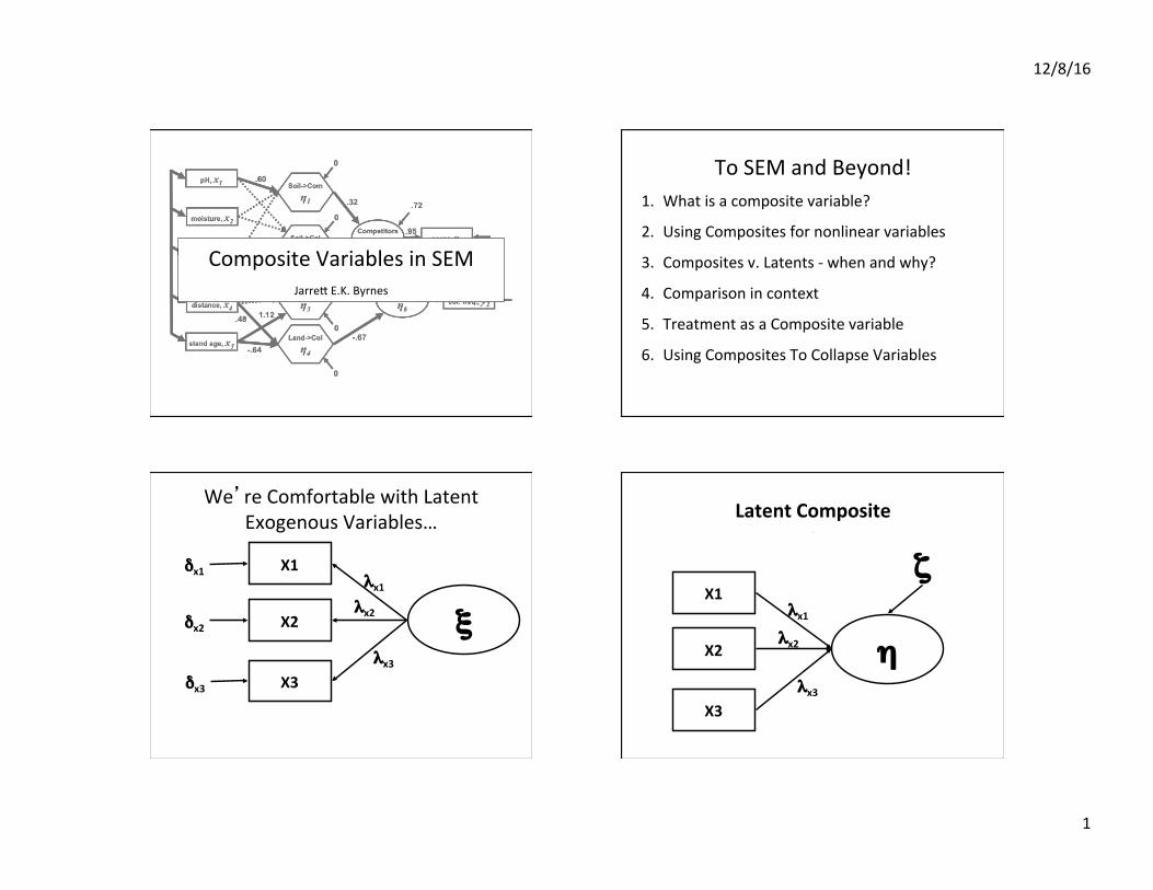
CompositeVariablesinSEM

Jarre9E.K.Byrnes

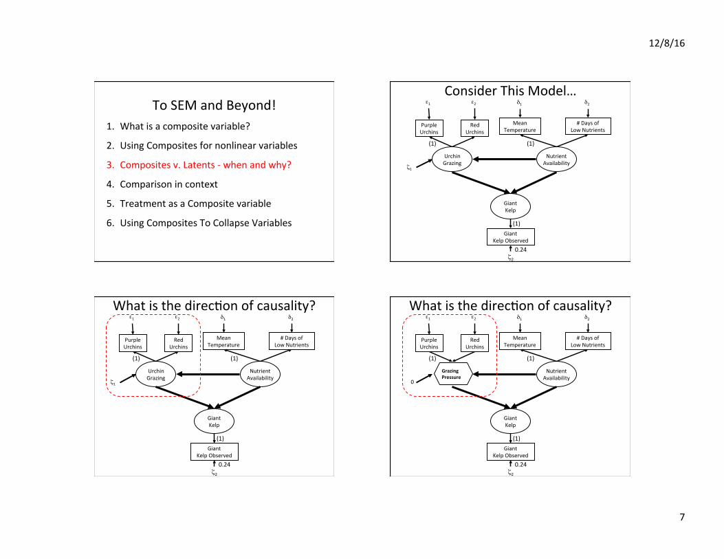
ToSEMandBeyond!1.  Whatisacompositevariable?

2.  UsingCompositesfornonlinearvariables

3.  Compositesv.Latents-whenandwhy?

4.  Comparisonincontext

5.  TreatmentasaCompositevariable

6.  UsingCompositesToCollapseVariables

We’reComfortablewithLatentExogenousVariables…

ξ

X1δx1

X2

X3

δx2

δx3

λx1λx2

λx3

AndNow,LatentVariablesDrivenbyObservedExogenousCauses

η

X1

X2

X3

λx1λx2

λx3

ζ

LatentComposite

12/8/16

2

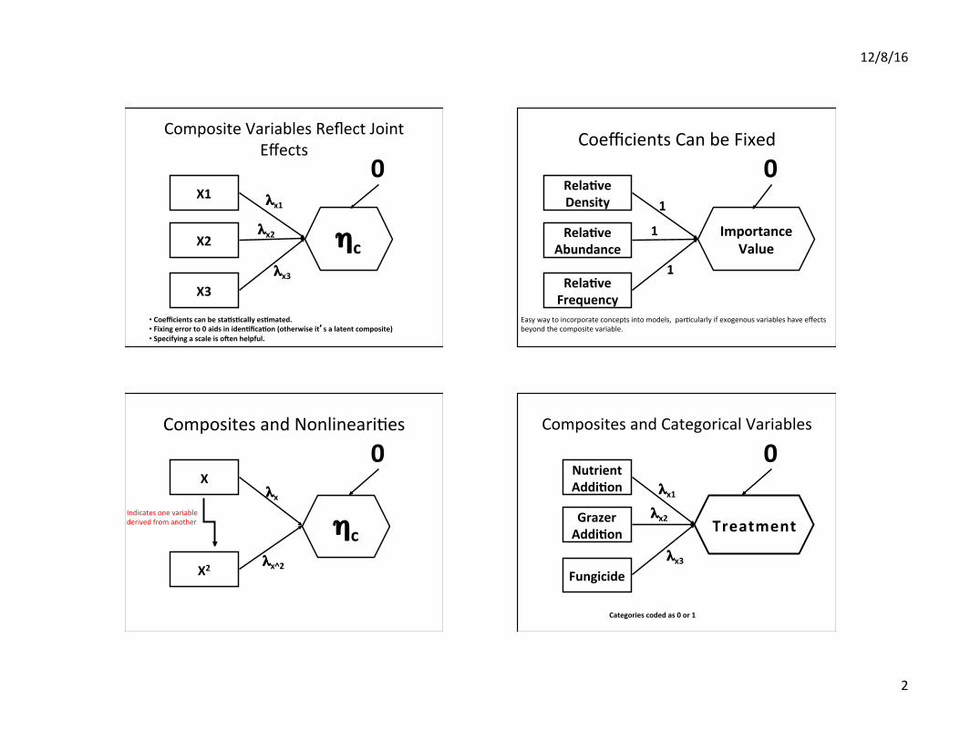
CompositeVariablesReflectJointEffects

X1

X2

X3

λx1

λx2

λx3

0

ηc

• Coefficientscanbesta6s6callyes6mated.• Fixingerrorto0aidsiniden6fica6on(otherwiseit’salatentcomposite)• SpecifyingascaleisoEenhelpful.

CoefficientsCanbeFixed

Rela6veDensity

Rela6veAbundance

Rela6veFrequency

11

1

0

ImportanceValue

Easywaytoincorporateconceptsintomodels,par\cularlyifexogenousvariableshaveeffectsbeyondthecompositevariable.

CompositesandNonlineari\es

X

X2

λx

λx^2

0

Indicatesonevariablederivedfromanother ηc

CompositesandCategoricalVariables

NutrientAddi6on

GrazerAddi6on

Fungicide

λx1

λx2

λx3

0

Categoriescodedas0or1

Treatment

12/8/16

3

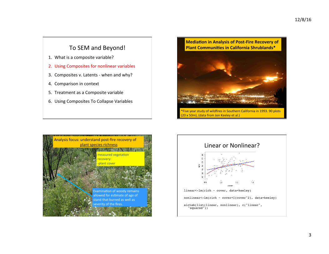
ToSEMandBeyond!1.  Whatisacompositevariable?

2.  UsingCompositesfornonlinearvariables

3.  Compositesv.Latents-whenandwhy?

4.  Comparisonincontext

5.  TreatmentasaCompositevariable

6.  UsingCompositesToCollapseVariables

10

Media6oninAnalysisofPost-FireRecoveryofPlantCommuni6esinCaliforniaShrublands*

*FiveyearstudyofwildfiresinSouthernCaliforniain1993.90plots(20x50m),(datafromJonKeeleyetal.)

11

Analysisfocus:understandpost-firerecoveryofplantspeciesrichness

Examina\onofwoodyremainsallowedfores\mateofageofstandthatburnedaswellasseverityofthefires.

measuredvegeta\onrecovery:- plantcover- speciesrichness

linear<-lm(rich ~ cover, data=keeley)

nonlinear<-lm(rich ~ cover+I(cover^2), data=keeley)

aictab(list(linear, nonlinear), c("linear", "squared"))

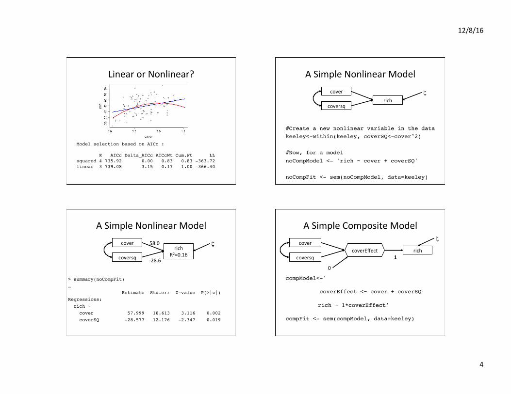
LinearorNonlinear?

12/8/16

4

Model selection based on AICc :

K AICc Delta_AICc AICcWt Cum.Wt LLsquared 4 735.92 0.00 0.83 0.83 -363.72linear 3 739.08 3.15 0.17 1.00 -366.40

LinearorNonlinear? ASimpleNonlinearModel

#Create a new nonlinear variable in the datakeeley<-within(keeley, coverSQ<-cover^2)

#Now, for a modelnoCompModel <- 'rich ~ cover + coverSQ'

noCompFit <- sem(noCompModel, data=keeley)

cover

richcoversq

ζ

ASimpleNonlinearModel

> summary(noCompFit)… Estimate Std.err Z-value P(>|z|)Regressions: rich ~ cover 57.999 18.613 3.116 0.002 coverSQ -28.577 12.176 -2.347 0.019

coverrich

R2=0.16coversq

58.0

-28.6

ζ

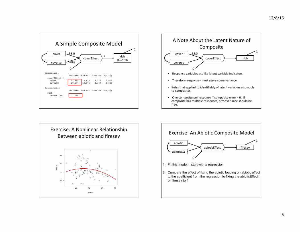
ASimpleCompositeModel

compModel<-'

coverEffect <~ cover + coverSQ

rich ~ 1*coverEffect'

compFit <- sem(compModel, data=keeley)

richcover

coversqcoverEffect

0

ζ

1

12/8/16

5

ASimpleCompositeModel

Composites: Estimate Std.Err Z-value P(>|z|) coverEffect <~ cover 57.999 18.613 3.116 0.002 coverSQ -28.577 12.176 -2.347 0.019

Regressions: Estimate Std.Err Z-value P(>|z|) rich ~ coverEffect 1.000

richR2=0.16

cover

coversqcoverEffect

0

-28.6

158.0

ζ

ANoteAbouttheLatentNatureofComposite

•  Responsevariablesactlikelatentvariableindicators

•  Therefore,responsesmustsharesomevariance.

•  Rulesthatappliedtoiden\fiablyoflatentvariablesalsoapplytocomposites.

•  Onecompositeperresponseifcompositeerror=0.Ifcompositehasmul\pleresponses,errorvarianceshouldbefree.

richcover

coversqcoverEffect

0

58.0ζ

Exercise:ANonlinearRela\onshipBetweenabio\candfiresev Exercise:AnAbio\cCompositeModel

1.  Fit this model – start with a regression

2.  Compare the effect of fixing the abiotic loading on abiotic effect to the coefficient from the regression to fixing the abioticEffect on firesev to 1.

firesevabio\c

abio\cSQabio\cEffect

0

ζ

12/8/16

6

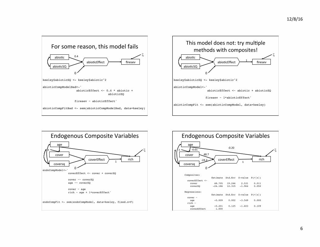
Forsomereason,thismodelfails

keeley$abioticSQ <- keeley$abiotic^2

abioticCompModelBad<-' abioticEffect <~ 0.4 * abiotic +

abioticSQ

firesev ~ abioticEffect'

abioticCompFitBad <- sem(abioticCompModelBad, data=keeley)

firesevabio\c

abio\cSQabio\cEffect

0.4

0

ζ

Thismodeldoesnot:trymul\plemethodswithcomposites!

keeley$abioticSQ <- keeley$abiotic^2

abioticCompModel<-' abioticEffect <~ abiotic + abioticSQ

firesev ~ 1*abioticEffect'

abioticCompFit <- sem(abioticCompModel, data=keeley)

firesevabio\c

abio\cSQabio\cEffect 1

0

ζ

EndogenousCompositeVariables

endoCompModel<-' coverEffect <~ cover + coverSQ

cover ~~ coverSQ age ~~ coverSQ

cover ~ age rich ~ age + 1*coverEffect'

endoCompFit <- sem(endoCompModel, data=keeley, fixed.x=F)

richcover

coversqcoverEffect

0

age

δ ζ

1

EndogenousCompositeVariables

Composites: Estimate Std.Err Z-value P(>|z|) coverEffect <~ cover 48.705 19.246 2.531 0.011 coverSQ -24.186 12.315 -1.964 0.050

Regressions: Estimate Std.Err Z-value P(>|z|) cover ~ age -0.009 0.002 -3.549 0.000 rich ~ age -0.201 0.125 -1.603 0.109 coverEffect 1.000

richcover

coversqcoverEffect

48.7

0

age

δ ζ

1

-0.20

-24.2

-0.01

12/8/16

7

ToSEMandBeyond!1.  Whatisacompositevariable?

2.  UsingCompositesfornonlinearvariables

3.  Compositesv.Latents-whenandwhy?

4.  Comparisonincontext

5.  TreatmentasaCompositevariable

6.  UsingCompositesToCollapseVariables

ConsiderThisModel…

UrchinGrazing

NutrientAvailability

GiantKelp

PurpleUrchins

RedUrchins

MeanTemperature

#DaysofLowNutrients

GiantKelpObserved

ε1 ε2

ζ2

δ1 δ2

ζ1

(1)

(1) (1)

0.24

UrchinGrazing

NutrientAvailability

GiantKelp

PurpleUrchins

RedUrchins

MeanTemperature

#DaysofLowNutrients

GiantKelpObserved

ε1 ε2 δ1 δ2

ζ1

(1)

(1) (1)

Whatisthedirec\onofcausality?

ζ20.24

Whatisthedirec\onofcausality?

NutrientAvailability

GiantKelp

PurpleUrchins

RedUrchins

MeanTemperature

#DaysofLowNutrients

GiantKelpObserved

ε1 ε2 δ1 δ2

0

(1)

(1) (1)

GrazingPressure

ζ20.24

12/8/16

8

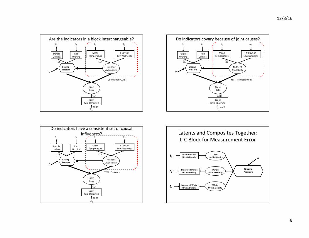
Aretheindicatorsinablockinterchangeable?

NutrientAvailability

GiantKelp

PurpleUrchins

RedUrchins

MeanTemperature

#DaysofLowNutrients

GiantKelpObserved

ε1 ε2 δ1 δ2

0

(1)

(1) (1)

GrazingPressure

Correla\on=0.78

ζ20.24

Doindicatorscovarybecauseofjointcauses?

NutrientAvailability

GiantKelp

PurpleUrchins

RedUrchins

MeanTemperature

#DaysofLowNutrients

GiantKelpObserved

ε1 ε2 δ1 δ2

0

(1)

(1) (1)

GrazingPressure

YES!Temperature!

ζ20.24

Doindicatorshaveaconsistentsetofcausalinfluences?

NutrientAvailability

GiantKelp

PurpleUrchins

RedUrchins

MeanTemperature

#DaysofLowNutrients

GiantKelpObserved

ε1 ε2 δ1 δ2

0

(1)

(1) (1)

GrazingPressure

YES!Currents!

ζ20.24

LatentsandCompositesTogether:L-CBlockforMeasurementError

GrazingPressure

δ1

δ2

δ3

RedUrchinDensity

MeasuredRedUrchinDensity

MeasuredPurpleUrchinDensity

MeasuredWhiteUrchinDensity

PurpleUrchinDensity

0

WhiteUrchinDensity

12/8/16

9

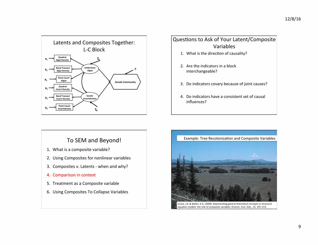
LatentsandCompositesTogether:L-CBlock

SessileCommunity

ε1

ε2

ε3

UnderstoryAlgae

QuadratAlgalDensity

BandTransectAlgalDensity

PointCountAlgae

ζ1

SessileInvertebrates

QuadratInvertDensity

BandTransectInvertDensity

PointCountInvertebrates

ε4

ε5

ε6 ζ2

0

Ques\onstoAskofYourLatent/CompositeVariables

1.  Whatisthedirec\onofcausality?

2.  Aretheindicatorsinablockinterchangeable?

3.  Doindicatorscovarybecauseofjointcauses?

4.  Doindicatorshaveaconsistentsetofcausalinfluences?

ToSEMandBeyond!1.  Whatisacompositevariable?

2.  UsingCompositesfornonlinearvariables

3.  Compositesv.Latents-whenandwhy?

4.  Comparisonincontext

5.  TreatmentasaCompositevariable

6.  UsingCompositesToCollapseVariables

Grace,J.B.&Bollen,K.A.(2008).Represen\nggeneraltheore\calconceptsinstructuralequa\onmodels:theroleofcompositevariables.Environ.Ecol.Stat.,15,191–213.

Example:TreeRecoloniza\onandCompositeVariables

12/8/16

10

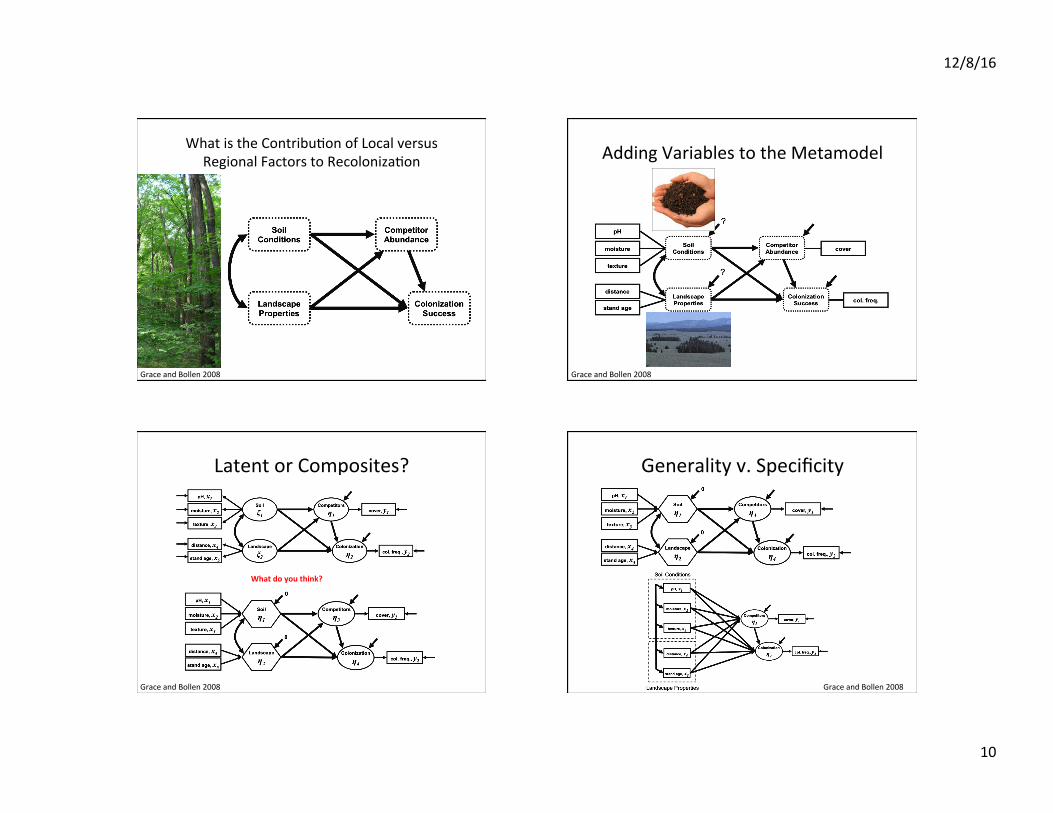
WhatistheContribu\onofLocalversusRegionalFactorstoRecoloniza\on

GraceandBollen2008

AddingVariablestotheMetamodel

GraceandBollen2008

LatentorComposites?

GraceandBollen2008

Whatdoyouthink?

Generalityv.Specificity

GraceandBollen2008

12/8/16

11

Generalityv.Specificity

GraceandBollen2008

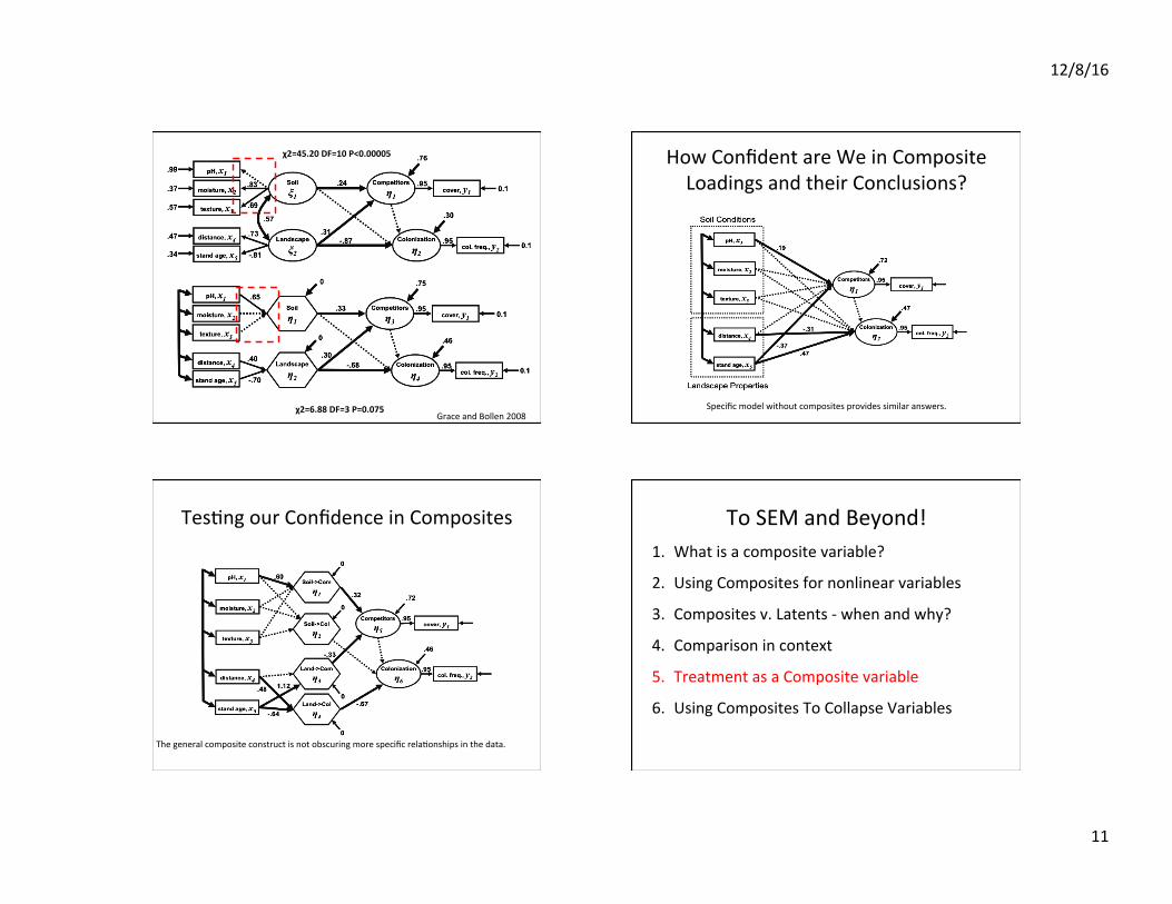
χ2=45.20DF=10P<0.00005

χ2=6.88DF=3P=0.075

HowConfidentareWeinCompositeLoadingsandtheirConclusions?

Specificmodelwithoutcompositesprovidessimilaranswers.

Tes\ngourConfidenceinComposites

Thegeneralcompositeconstructisnotobscuringmorespecificrela\onshipsinthedata.

ToSEMandBeyond!1.  Whatisacompositevariable?

2.  UsingCompositesfornonlinearvariables

3.  Compositesv.Latents-whenandwhy?

4.  Comparisonincontext

5.  TreatmentasaCompositevariable

6.  UsingCompositesToCollapseVariables

12/8/16

12

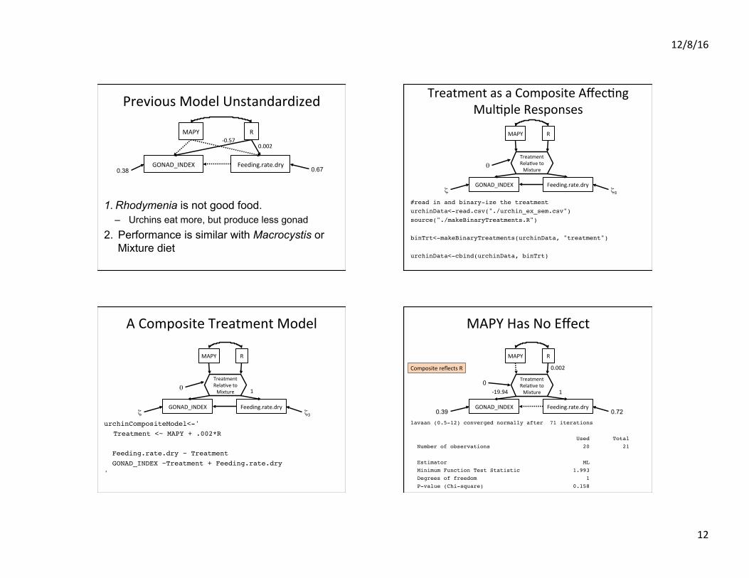
PreviousModelUnstandardized

1. Rhodymenia is not good food. –  Urchins eat more, but produce less gonad

2.  Performance is similar with Macrocystis or Mixture diet

MAPY

Feeding.rate.dryGONAD_INDEX

R

0.67 0.38

0.002-0.57

TreatmentasaCompositeAffec\ngMul\pleResponses

#read in and binary-ize the treatmenturchinData<-read.csv("./urchin_ex_sem.csv")source("./makeBinaryTreatments.R")

binTrt<-makeBinaryTreatments(urchinData, "treatment")

urchinData<-cbind(urchinData, binTrt)

MAPY

Feeding.rate.dryGONAD_INDEX

R

ζ3ζ

TreatmentRela\vetoMixture

0

ACompositeTreatmentModel

urchinCompositeModel<-' Treatment <~ MAPY + .002*R

Feeding.rate.dry ~ Treatment GONAD_INDEX ~Treatment + Feeding.rate.dry'

MAPY

Feeding.rate.dryGONAD_INDEX

R

ζ3ζ

TreatmentRela\vetoMixture

0 1

MAPYHasNoEffect

lavaan (0.5-12) converged normally after 71 iterations

Used Total Number of observations 20 21

Estimator ML Minimum Function Test Statistic 1.993 Degrees of freedom 1 P-value (Chi-square) 0.158

MAPY

Feeding.rate.dryGONAD_INDEX

R

0.72 0.39

TreatmentRela\vetoMixture

0.002

0

1-19.94

CompositereflectsR

12/8/16

13

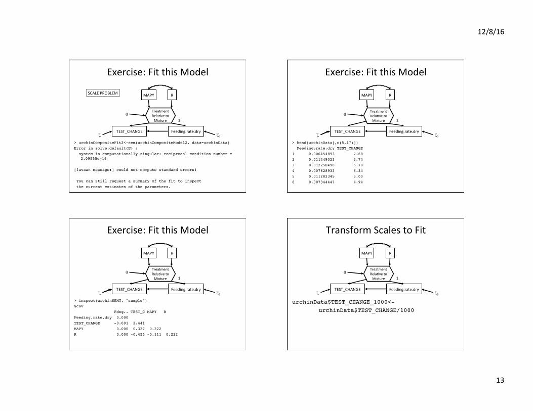
Exercise:FitthisModel

> urchinCompositeFit2<-sem(urchinCompositeModel2, data=urchinData)Error in solve.default(E) : system is computationally singular: reciprocal condition number =

2.09555e-16

[lavaan message:] could not compute standard errors!

You can still request a summary of the fit to inspect the current estimates of the parameters.

MAPY

Feeding.rate.dryTEST_CHANGE

R

ζ3ζ

TreatmentRela\vetoMixture

0

SCALEPROBLEM

1

Exercise:FitthisModel

> head(urchinData[,c(5,17)]) Feeding.rate.dry TEST_CHANGE1 0.006454893 7.682 0.011449023 3.743 0.012258490 5.784 0.007628933 6.345 0.011282345 5.006 0.007344447 4.94

MAPY

Feeding.rate.dry

R

ζ3ζ

TreatmentRela\vetoMixture

0

TEST_CHANGE

1

Exercise:FitthisModel

> inspect(urchinSEMT, "sample")$cov Fdng.. TEST_C MAPY R Feeding.rate.dry 0.000 TEST_CHANGE -0.001 2.441 MAPY 0.000 0.322 0.222 R 0.000 -0.455 -0.111 0.222

MAPY

Feeding.rate.dry

R

ζ3ζ

TreatmentRela\vetoMixture

0

TEST_CHANGE

1

TransformScalestoFit

urchinData$TEST_CHANGE_1000<-urchinData$TEST_CHANGE/1000

MAPY

Feeding.rate.dry

R

ζ3ζ

TreatmentRela\vetoMixture 1

0

TEST_CHANGE

12/8/16

14

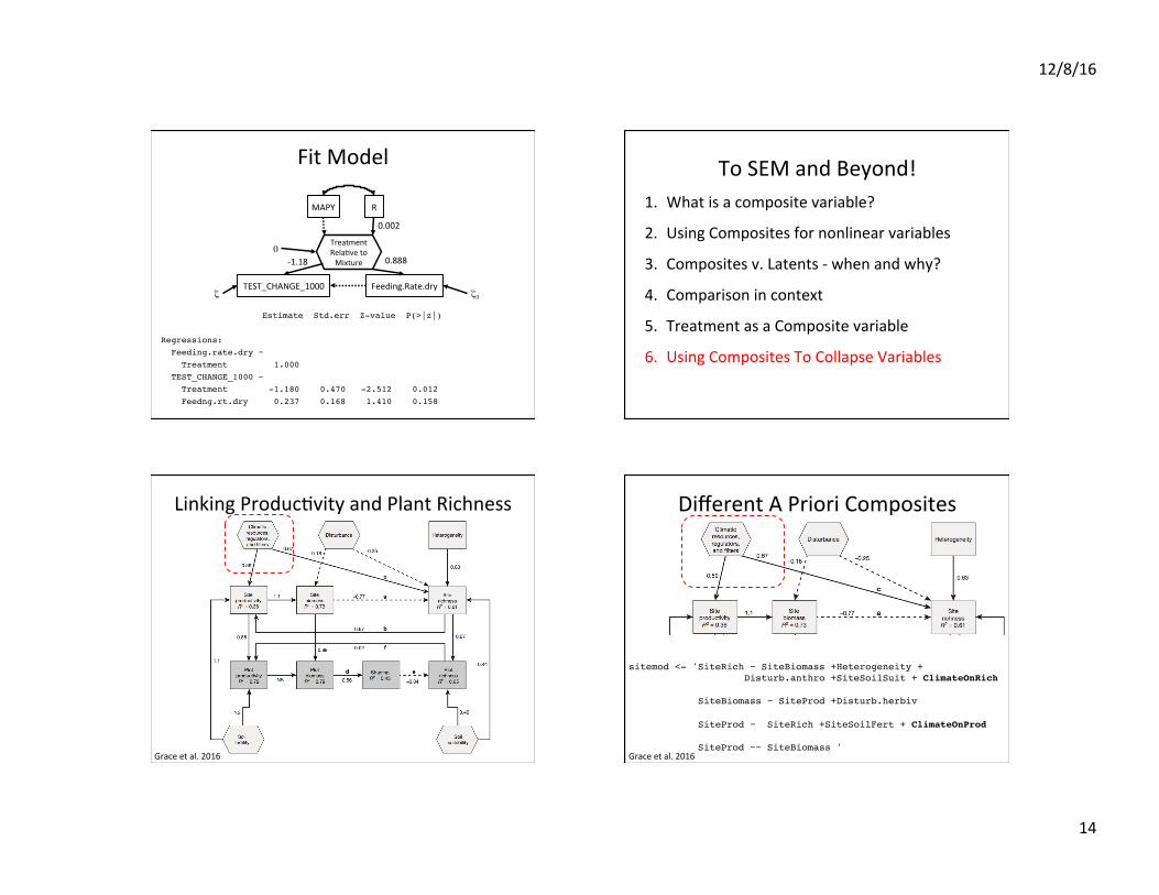
FitModel

Estimate Std.err Z-value P(>|z|)

Regressions: Feeding.rate.dry ~ Treatment 1.000 TEST_CHANGE_1000 ~ Treatment -1.180 0.470 -2.512 0.012 Feedng.rt.dry 0.237 0.168 1.410 0.158

MAPY

Feeding.Rate.dry

R

ζ3ζ

TreatmentRela\vetoMixture

0.002

0

TEST_CHANGE_1000

-1.18 0.888

ToSEMandBeyond!1.  Whatisacompositevariable?

2.  UsingCompositesfornonlinearvariables

3.  Compositesv.Latents-whenandwhy?

4.  Comparisonincontext

5.  TreatmentasaCompositevariable

6.  UsingCompositesToCollapseVariables

LinkingProduc\vityandPlantRichness

Graceetal.2016

DifferentAPrioriComposites

sitemod <- 'SiteRich ~ SiteBiomass +Heterogeneity +Disturb.anthro +SiteSoilSuit + ClimateOnRich

SiteBiomass ~ SiteProd +Disturb.herbiv

SiteProd ~ SiteRich +SiteSoilFert + ClimateOnProd

SiteProd ~~ SiteBiomass 'Graceetal.2016

12/8/16

15

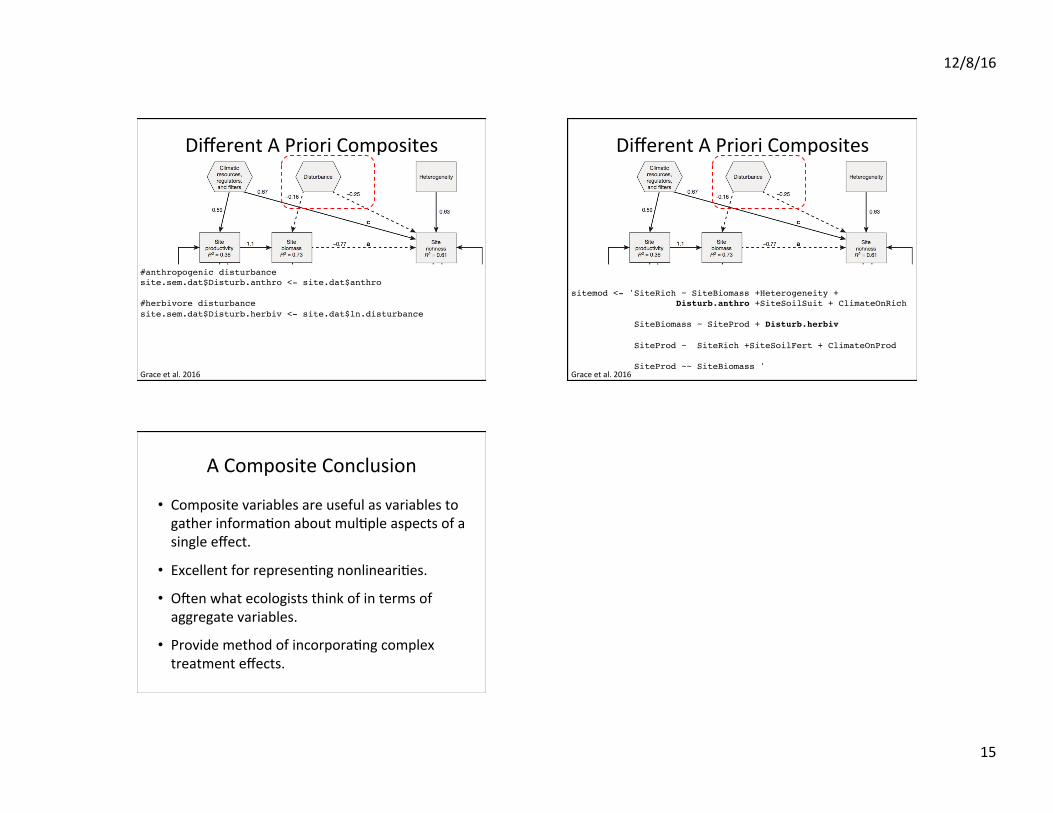
DifferentAPrioriComposites

Graceetal.2016

#anthropogenic disturbancesite.sem.dat$Disturb.anthro <- site.dat$anthro

#herbivore disturbancesite.sem.dat$Disturb.herbiv <- site.dat$ln.disturbance

DifferentAPrioriComposites

sitemod <- 'SiteRich ~ SiteBiomass +Heterogeneity +Disturb.anthro +SiteSoilSuit + ClimateOnRich

SiteBiomass ~ SiteProd + Disturb.herbiv

SiteProd ~ SiteRich +SiteSoilFert + ClimateOnProd

SiteProd ~~ SiteBiomass 'Graceetal.2016

ACompositeConclusion

•  Compositevariablesareusefulasvariablestogatherinforma\onaboutmul\pleaspectsofasingleeffect.

•  Excellentforrepresen\ngnonlineari\es.

•  Otenwhatecologiststhinkofintermsofaggregatevariables.

•  Providemethodofincorpora\ngcomplextreatmenteffects.