Theory of Vortex Sound - The Library of...

CB461-FM Howe June 6, 2002 14:18 Char Count=

Theory of Vortex Sound

M. S. HOWEBoston University

v


published by the press syndicate of the university of cambridgeThe Pitt Building, Trumpington Street, Cambridge, United Kingdom

cambridge university pressThe Edinburgh Building, Cambridge CB2 2RU, UK

40 West 20th Street, New York, NY 10011-4211, USA477 Williamstown Road, Port Melbourne, VIC 3207, Australia

Ruiz de Alarcon 13, 28014 Madrid, SpainDock House, The Waterfront, Cape Town 8001, South Africa

http://www.cambridge.org

c© Cambridge University Press 2003

This book is in copyright. Subject to statutory exceptionand to the provisions of relevant collective licensing agreements,

no reproduction of any part may take place withoutthe written permission of Cambridge University Press.

First published 2003

Printed in the United Kingdom at the University Press, Cambridge

Typeface Times Roman 10/13 pt. System LATEX [tb]

A catalog record for this book is available from the British Library.

Library of Congress Cataloging in Publication Data

Howe, M. S.

Theory of vortex sound / M. S. Howe.

p. cm. – (Cambridge texts in applied mathematics)

Includes bibliographical references and index.

ISBN 0-521-81281-X – ISBN 0-521-01223-6 (pbk.)

1. Fluid dynamics. 2. Fluids – Acoustic properties. I. Title. II. Series.

TA357.H69 2003

620.1′064 – dc21 2002022280

ISBN 0 521 81281 X hardbackISBN 0 521 01223 6 paperback

vi


Contents

Preface page xiii

1 Introduction 11.1 What is Vortex Sound? 11.2 Equations of Motion of a Fluid 21.3 Equation of Linear Acoustics 41.4 The Special Case of an Incompressible Fluid 71.5 Sound Produced by an Impulsive Point Source 101.6 Free-Space Green’s Function 121.7 Monopoles, Dipoles, and Quadrupoles 131.8 Acoustic Energy Flux 181.9 Calculation of the Acoustic Far Field 20Problems 1 23

2 Lighthill’s Theory 252.1 The Acoustic Analogy 252.2 Lighthill’s v8 Law 292.3 Curle’s Theory 322.4 Sound Produced by Turbulence Near a Compact Rigid Body 362.5 Radiation from a Noncompact Surface 37Problems 2 39

3 The Compact Green’s Function 413.1 The Influence of Solid Boundaries 413.2 The Helmholtz Equation 443.3 The Reciprocal Theorem 463.4 Time-Harmonic Compact Green’s Function 49

ix


x Contents

3.5 Compact Green’s Function for a Rigid Sphere 533.6 Compact Green’s Function for Cylindrical Bodies 583.7 Symmetric Compact Green’s Function 633.8 Low-Frequency Radiation from a Vibrating Body 653.9 Compact Green’s Function Summary and Special Cases 70Problems 3 79

4 Vorticity 824.1 Vorticity and the Kinetic Energy of Incompressible Flow 824.2 The Vorticity Equation 844.3 The Biot–Savart Law 884.4 Surface Force in Incompressible Flow Expressed in Terms

of Vorticity 934.5 The Complex Potential 1004.6 Motion of a Line Vortex 106Problems 4 112

5 Vortex Sound 1145.1 The Role of Vorticity in Lighthill’s Theory 1145.2 The Equation of Vortex Sound 1165.3 Vortex–Surface Interaction Noise 1245.4 Radiation from an Acoustically Compact Body 1285.5 Radiation from Cylindrical Bodies of Compact Cross Section 1305.6 Impulse Theory of Vortex Sound 131Problems 5 132

6 Vortex–Surface Interaction Noise in Two Dimensions 1366.1 Compact Green’s Function in Two Dimensions 1366.2 Sound Generated by a Line Vortex Interacting with

a Cylindrical Body 1396.3 Influence of Vortex Shedding 1456.4 Blade–Vortex Interaction Noise in Two Dimensions 150Problems 6 154

7 Problems in Three Dimensions 1567.1 Linear Theory of Vortex–Airfoil Interaction Noise 1567.2 Blade–Vortex Interactions in Three Dimensions 1587.3 Sound Produced by Vortex Motion near a Sphere 1627.4 Compression Wave Generated When a Train Enters a Tunnel 166Problems 7 172


Contents xi

8 Further Worked Examples 1758.1 Blade–Vortex Interactions in Two Dimensions 1758.2 Parallel Blade–Vortex Interactions in Three Dimensions 1868.3 Vortex Passing over a Spoiler 1918.4 Bluff Body Interactions: The Circular Cylinder 1948.5 Vortex Ring and Sphere 1998.6 Vortex Pair Incident on a Wall Aperture 204

Bibliography 209Index 213

CB461-01 Howe May 17, 2002 18:43 Char Count=

1Introduction

1.1 What is Vortex Sound?

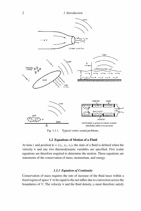
Vortex sound is the sound produced as a by-product of unsteady fluid mo-tions (Fig. 1.1.1). It is part of the more general subject of aerodynamic sound.The modern theory of aerodynamic sound was pioneered by James Lighthillin the early 1950s. Lighthill (1952) wanted to understand the mechanisms ofnoise generation by the jet engines of new passenger jet aircraft that werethen about to enter service. However, it is now widely recognized that anymechanism that produces sound can actually be formulated as a problem ofaerodynamic sound. Thus, apart from the high speed turbulent jet – which maybe regarded as a distribution of intense turbulence velocity fluctuations that gen-erate sound by converting a tiny fraction of the jet rotational kinetic energy intothe longitudinal waves that constitute sound – colliding solid bodies, aeroenginerotor blades, vibrating surfaces, complex fluid–structure interactions in the lar-ynx (responsible for speech), musical instruments, conventional loudspeakers,crackling paper, explosions, combustion and combustion instabilities in rock-ets, and so forth all fall within the theory of aerodynamic sound in its broadestsense.

In this book we shall consider principally the production of sound by un-steady motions of a fluid. Any fluid that possesses intrinsic kinetic energy, thatis, energy not directly attributable to a moving boundary (which is largely with-drawn from the fluid when the boundary motion ceases), must possess vorticity.We shall see that in a certain sense and for a vast number of flows vorticity maybe regarded as the ultimate source of the sound generated by the flow. Ourobjective, therefore, is to simplify the general aerodynamic sound problem toobtain a thorough understanding of how this happens, and of how the soundcan be estimated quantitatively.

1


2 1 Introduction

Fig. 1.1.1. Typical vortex sound problems.

1.2 Equations of Motion of a Fluid

At time t and position x = (x1, x2, x3), the state of a fluid is defined when thevelocity v and any two thermodynamic variables are specified. Five scalarequations are therefore required to determine the motion. These equations arestatements of the conservation of mass, momentum, and energy.

1.2.1 Equation of Continuity

Conservation of mass requires the rate of increase of the fluid mass within afixed region of space V to be equal to the net influx due to convection across theboundaries of V. The velocity v and the fluid density ρ must therefore satisfy


1.2 Equations of Motion of a Fluid 3

the equation of continuity, which has the following equivalent forms

∂ρ

∂t+ div(ρv) = 0,

1

ρ

Dρ

Dt+ div v = 0,

div v = ρD

Dt

(1

ρ

)

, (1.2.1)

where

D

Dt= ∂

∂t+ v · ∇ ≡ ∂

∂t+ v j

∂

∂x j(1.2.2)

is the material derivative; the repeated suffix j implies summation over j =1, 2, 3. The last of Equations (1.2.1) states that div v is equal to the rate ofchange of fluid volume per unit volume following the motion of the fluid. Foran incompressible fluid this is zero, i.e., div v = 0.

1.2.2 Momentum Equation

The momentum equation is also called the Navier–Stokes equation; it expressesthe rate of change of momentum of a fluid particle in terms of the pressure p,the viscous or frictional force, and body forces F per unit volume. We consideronly Stokesian fluids (most liquids and monatomic gases, but also a good ap-proximation in air for calculating the frictional drag at a solid boundary) forwhich the principal frictional forces are expressed in terms of the shear coeffi-cient of viscosity η, which we shall invariably assume to be constant. Then themomentum equation is

ρDvDt

= −∇ p + η

(∇2v + 1

3∇(div v)

)+ F. (1.2.3)

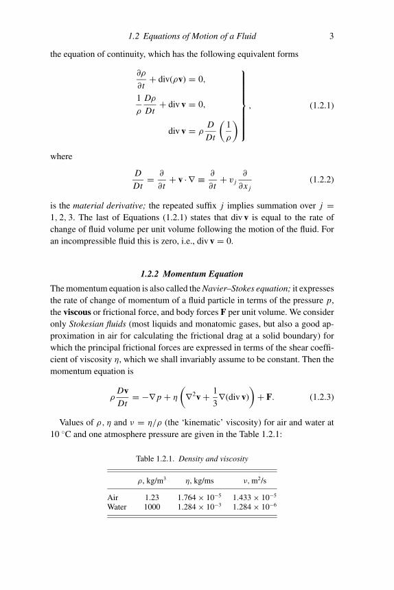
Values of ρ, η and ν = η/ρ (the ‘kinematic’ viscosity) for air and water at10 ◦C and one atmosphere pressure are given in the Table 1.2.1:

Table 1.2.1. Density and viscosity

ρ, kg/m3 η, kg/ms ν, m2/s

Air 1.23 1.764 × 10−5 1.433 × 10−5

Water 1000 1.284 × 10−3 1.284 × 10−6


4 1 Introduction

1.2.3 Energy Equation

This equation must be used in its full generality in problems where energy istransferred by heat conduction, where frictional dissipation of sound is occur-ring, when shock waves are formed by highly nonlinear events, or when soundis being generated by combustion and other heat sources. For our purposes itwill usually be sufficient to suppose the flow to be homentropic; namely, thespecific entropy s of the fluid is uniform and constant throughout the fluid, sothat the energy equation becomes

s = constant. (1.2.4)

We may then assume that the pressure and density are related by an equationof the form

p = p(ρ, s), s = constant. (1.2.5)

This equation will be satisfied by both the mean (undisturbed) and unsteadycomponents of the flow. Thus, for an ideal gas

p = constant × ργ , γ = ratio of specific heats. (1.2.6)

1.3 Equation of Linear Acoustics

The intensity of a sound pressure p in air is usually measured on a decibel scaleby the quantity

20 × log10

( |p|pref

),

where the reference pressure pref = 2 × 10−5 N/m2. Thus, p = p0 ≡ 1 atmo-sphere ( = 105 N/m2) is equivalent to 194 dB. A very loud sound ∼120 dBcorresponds to

p

p0≈ 2 × 10−5

105× 10( 120

20 ) = 2 × 10−4 1.

Similarly, for a ‘deafening’ sound of 160 dB, p/p0 ∼ 0.02. This correspondsto a pressure of about 0.3 lbs/in2 and is loud enough for nonlinear effects tobegin to be important.

The passage of a sound wave in the form of a pressure fluctuation is, ofcourse, accompanied by a back-and-forth motion of the fluid at the acoustic


1.3 Equation of Linear Acoustics 5

particle velocity v, say. We shall see later that

acoustic particle velocity ≈ acoustic pressure

mean density × speed of sound.

In air the speed of sound is about 340 m/sec. Thus, at 120 dB v ∼ 5 cm/sec; at160 dB v ∼ 5 m/sec.

In most applications the acoustic amplitude is very small relative to the meanpressure p0, and sound propagation may be studied by linearizing the equations.To do this we shall first consider sound propagating in a stationary inviscid fluidof mean pressure p0 and density ρ0; let the departures of the pressure and densityfrom these mean values be denoted by p′, ρ ′, where p′/p0 1, ρ ′/ρ0 1. Thelinearized momentum equation (1.2.3) becomes

ρ0∂v∂t

+ ∇ p′ = F. (1.3.1)

Before linearizing the continuity equation (1.2.1), we introduce an artificialgeneralization by inserting a volume source distribution q(x, t) on the right-hand side

1

ρ

Dρ

Dt+ div v = q, (1.3.2)

where q is the rate of increase of fluid volume per unit volume of the fluid, andmight represent, for example, the effect of volume pulsations of a small bodyin the fluid. The linearized equation is then

1

ρ0

∂ρ ′

∂t+ div v = q. (1.3.3)

Now eliminate v between (1.3.1) and (1.3.3):

∂2ρ ′

∂t2− ∇2 p′ = ρ0

∂q

∂t− div F. (1.3.4)

An equation determining the pressure p′ alone in terms of q and F is obtainedby invoking the homentropic relation (1.2.5). In the undisturbed and disturbedstates we have

p0 = p(ρ0, s), p0 + p′ = p(ρ0 + ρ ′, s) ≈ p(ρ0, s) +(

∂p

∂ρ(ρ, s)

)0

ρ ′,

s = constant. (1.3.5)


6 1 Introduction

The derivative is evaluated at the undisturbed values of the pressure and density(p0, ρ0). It has the dimensions of velocity2, and its square root defines the speedof sound

c0 =√(

∂p

∂ρ

)s

, (1.3.6)

where the derivative is taken with the entropy s held fixed at its value in theundisturbed fluid. The implication is that losses due to heat transfer betweenneighboring fluid particles by viscous and thermal diffusion are neglectedduring the passage of a sound wave (i.e., that the motion of a fluid particleis adiabatic).

From (1.3.5): ρ ′ = p′/c20. Hence, substituting for ρ ′ in (1.3.4), we obtain(

1

c20

∂2

∂t2− ∇2

)p = ρ0

∂q

∂t− div F, (1.3.7)

where the prime (′) on the acoustic pressure has been discarded. This equationgoverns the production of sound waves by the volume source q and the forceF. When these terms are absent the equation describes sound propagationfrom sources on the boundaries of the fluid, such as the vibrating cone of aloudspeaker.

The volume source q and the body force F would never appear in a completedescription of sound generation within a fluid. They are introduced only whenwe think we understand how to model the real sources of sound in terms ofvolume sources and forces. In general this can be a dangerous procedure be-cause, as we shall see, small errors in specifying the sources of sound in a fluidcan lead to very large errors in the predicted sound. This is because only a tinyfraction of the available energy of a vibrating fluid or structure actually radiatesaway as sound.

When F = 0, Equation (1.3.1) implies the existence of a velocity potentialϕ such that v = ∇ϕ, in terms of which the perturbation pressure is given by

p = −ρ0∂ϕ

∂t. (1.3.8)

It follows from this and (1.3.7) (with F = 0) that the velocity potential is thesolution of (

1

c20

∂2

∂t2− ∇2

)ϕ = −q(x, t). (1.3.9)

This is the wave equation of classical acoustics.


1.4 The Special Case of an Incompressible Fluid 7

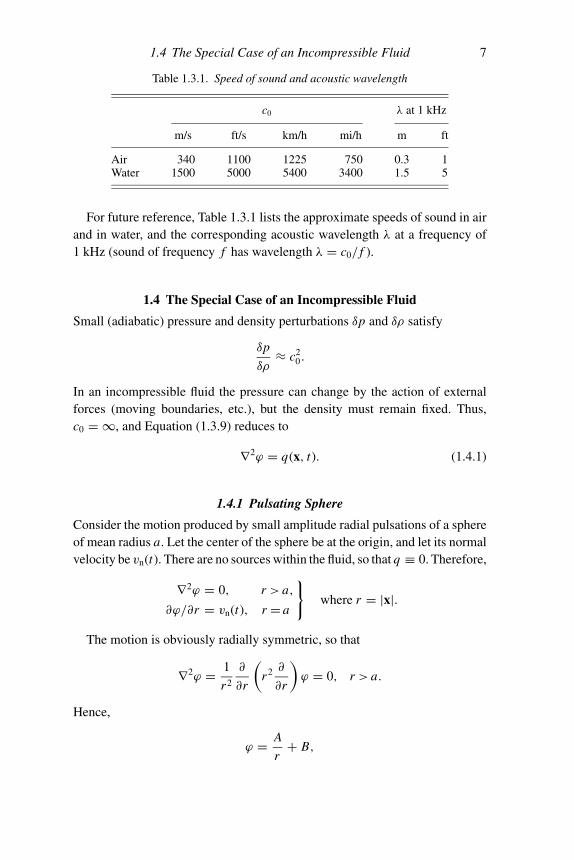
Table 1.3.1. Speed of sound and acoustic wavelength

c0 λ at 1 kHz

m/s ft/s km/h mi/h m ft

Air 340 1100 1225 750 0.3 1Water 1500 5000 5400 3400 1.5 5

For future reference, Table 1.3.1 lists the approximate speeds of sound in airand in water, and the corresponding acoustic wavelength λ at a frequency of1 kHz (sound of frequency f has wavelength λ = c0/ f ).

1.4 The Special Case of an Incompressible Fluid

Small (adiabatic) pressure and density perturbations δp and δρ satisfy

δp

δρ≈ c2

0.

In an incompressible fluid the pressure can change by the action of externalforces (moving boundaries, etc.), but the density must remain fixed. Thus,c0 = ∞, and Equation (1.3.9) reduces to

∇2ϕ = q(x, t). (1.4.1)

1.4.1 Pulsating Sphere

Consider the motion produced by small amplitude radial pulsations of a sphereof mean radius a. Let the center of the sphere be at the origin, and let its normalvelocity be vn(t). There are no sources within the fluid, so that q ≡ 0. Therefore,

∇2ϕ = 0, r > a,

∂ϕ/∂r = vn(t), r = a

}where r = |x|.

The motion is obviously radially symmetric, so that

∇2ϕ = 1

r2

∂

∂r

(r2 ∂

∂r

)ϕ = 0, r > a.

Hence,

ϕ = A

r+ B,


8 1 Introduction

where A ≡ A(t) and B ≡ B(t) are functions of t . B(t) can be discarded be-cause the pressure fluctuations (∼ −ρ0∂ϕ/∂t) must vanish as r → ∞. Apply-ing the condition ∂ϕ/∂r = vn at r = a, we then find

ϕ = −a2vn(t)

r, r > a. (1.4.2)

Thus, the pressure

p = −ρ0∂ϕ

∂t= ρ0

a2

r

dvn

dt(t)

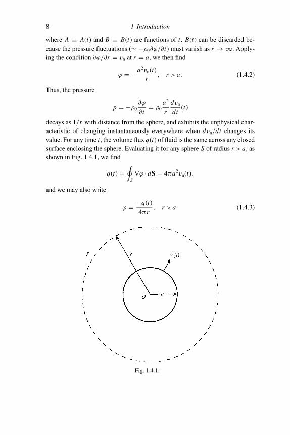
decays as 1/r with distance from the sphere, and exhibits the unphysical char-acteristic of changing instantaneously everywhere when dvn/dt changes itsvalue. For any time t , the volume flux q(t) of fluid is the same across any closedsurface enclosing the sphere. Evaluating it for any sphere S of radius r > a, asshown in Fig. 1.4.1, we find

q(t) =∮

S∇ϕ · dS = 4πa2vn(t),

and we may also write

ϕ = −q(t)

4πr, r > a. (1.4.3)

Fig. 1.4.1.


1.4 The Special Case of an Incompressible Fluid 9

1.4.2 Point Source

The incompressible motion generated by a volume point source of strength q(t)at the origin is the solution of

∇2ϕ = q(t)δ(x), where δ(x) = δ(x1)δ(x2)δ(x3). (1.4.4)

The solution must be radially symmetric and given by

ϕ = A

rfor r > 0. (1.4.5)

To find A, we integrate (1.4.4) over the interior of a sphere of radius r = R > 0,and use the divergence theorem

∫r<R ∇2ϕ d3x = ∮

S ∇ϕ · dS, where S is thesurface of the sphere. Then

∮S∇ϕ · dS ≡

(−A

R2

)× (4π R2) = q(t).

Hence, A = −q(t)/4π and ϕ = −q(t)/4πr , which agrees with the solution(1.4.3) for the sphere with the same volume outflow in the region r > a = radiusof the sphere. This indicates that when we are interested in modelling the effectof a pulsating sphere at large distances r � a, it is permissible to replace thesphere by a point source (a monopole) of the same strength q(t) = rate ofchange of the volume of the sphere. This conclusion is valid for any pulsatingbody, not just a sphere. However, it is not necessarily a good model (especiallywhen we come to examine the production of sound by a pulsating body) in thepresence of a mean fluid flow past the sphere.

The Solution (1.4.5) for the point source is strictly valid only for r > 0,where it satisfies ∇2ϕ = 0. What happens as r → 0, where its value is actuallyundefined? To answer this question, we write the solution in the form

ϕ = limε→0

−q(t)

4π (r2 + ε2)12

, ε > 0, in which case ∇2ϕ = limε→0

3ε2q(t)

4π (r2 + ε2)52

.

The last limit is just equal to q(t)δ(x). Indeed when ε is small 3ε2/4π (r2 + ε2)52

is also small except close to r = 0, where it attains a large maximum ∼3/4πε3.Therefore, for any smoothly varying test function f (x) and any volume V


10 1 Introduction

enclosing the origin

limε→0

∫V

3ε2 f (x) d3x

4π (r2 + ε2)52

= f (0) limε→0

∫ ∞

−∞

3ε2 d3x

4π (r2 + ε2)52

= f (0)∫ ∞

0

3ε2r2 dr

(r2 + ε2)52

= f (0),

where the value of the last integral is independent of ε. This is the definingproperty of the three-dimensional δ function.

Thus, the correct interpretation of the solution

ϕ = −1

4πrof ∇2ϕ = δ(x) (1.4.6)

for a unit point source (q = 1) is

−1

4πr= lim

ε→0

−1

4π (r2 + ε2)12

, r ≥ 0, (1.4.7)

where

∇2

( −1

4πr

)= lim

ε→0∇2

( −1

4π (r2 + ε2)12

)= lim

ε→0

3ε2

4π (r2 + ε2)52

= δ(x). (1.4.8)

1.5 Sound Produced by an Impulsive Point Source

The sound generated by the unit, impulsive point source δ(x)δ(t) is the solutionof (

1

c20

∂2

∂t2− ∇2

)ϕ = δ(x)δ(t). (1.5.1)

The source exists only for an infinitesimal instant of time at t = 0; therefore atearlier times ϕ(x, t) = 0 everywhere.

It is evident that the solution is radially symmetric, and that for r = |x| > 0we have to solve

1

c20

∂2ϕ

∂t2− 1

r2

∂

∂r

(r2 ∂

∂r

)ϕ = 0, r > 0. (1.5.2)

The identity

1

r2

∂

∂r

(r2 ∂

∂r

)ϕ ≡ 1

r

∂2

∂r2(rϕ) (1.5.3)


1.5 Sound Produced by an Impulsive Point Source 11

permits us to write Equation (1.5.2) in the form of the one-dimensional waveequation for rϕ:

1

c20

∂2

∂t2(rϕ) − ∂2

∂r2(rϕ) = 0, r > 0. (1.5.4)

This has the general solution rϕ = �(t − r/c0) + �(t + r/c0), where � and� are arbitrary functions. Hence, the general solution of (1.5.2) is

ϕ = �(t − r

c0

)r

+ �(t + r

c0

)r

, r > 0. (1.5.5)

The first term on the right represents a spherically symmetric disturbance thatpropagates in the direction of increasing values of r at the speed of sound c0 as tincreases, whereas the second represents an incoming wave converging towardx = 0. We must therefore set � = 0, since it represents sound waves generatedat r = ∞ that approach the source rather than sound waves generated by thesource and radiating away from the source. This is a causality or radiationcondition, that (in the absence of boundaries) sound produced by a sourcemust radiate away from the source. It is also consistent with the Second Lawof Thermodynamics, which requires natural systems to change in the moreprobable direction. An event in which sound waves converge on a point fromall directions at infinity is so unlikely as to be impossible in practice; it would bethe acoustic analogue of the far-scattered pieces of a broken cup spontaneouslyreassembling.

To complete the solution it remains to determine the function �. We do thisby extending the solution down to the source at r = 0 by writing (c.f., (1.4.7))

ϕ = �(t − r

c0

)r

= limε→0

�(t − r

c0

)(r2 + ε2)

12

, r ≥ 0. (1.5.6)

Let us substitute this into Equation (1.5.1) and examine what happens as ε → 0.By direct calculation we find

∇2ϕ = 1

r

∂2

∂r2(rϕ) = −3ε2�(t − r/c0)

(r2 + ε2)52

− 2ε2�′(t − r/c0)

c0r (r2 + ε2)32

+ �′′(t − r/c0)

c20(r2 + ε2)

12

1

c20

∂2ϕ

∂t2= �′′(t − r/c0)

c20(r2 + ε2)

12


12 1 Introduction

Therefore,

1

c20

∂2ϕ

∂t2− ∇2ϕ = 3ε2�(t − r/c0)

(r2 + ε2)52

+ 2ε2�′(t − r/c0)

c0r (r2 + ε2)32

→ 4π�(t)δ(x) + 0 as ε → 0, (1.5.7)

where the δ function in the last line follows from (1.4.8), and the ‘+ 0’ isobtained by noting that for any smoothly varying test function f (x) and anyvolume V enclosing the origin∫

V

2ε2 f (x) d3x

r (r2 + ε2)32

≈ f (0)∫ ∞

−∞

2ε2 d3x

r (r2 + ε2)32

= f (0)∫ ∞

0

8πε2r dr

(r2 + ε2)32

= 8πε f (0) → 0 as ε → 0.

Hence, comparing (1.5.7) with the inhomogeneous wave equation (1.5.1),we find

�(t) = 1

4πδ(t),

and the Solution (1.5.6) becomes

ϕ(x, t) = 1

4πrδ

(t − r

c0

)≡ 1

4π |x|δ(

t − |x|c0

). (1.5.8)

This represents a spherical pulse that is nonzero only on the surface of thesphere r = c0t > 0, whose radius increases at the speed of sound c0; it vanisheseverywhere for t < 0, before the impulsive source is triggered.

1.6 Free-Space Green’s Function

The free-space Green’s function G(x, y, t −τ ) is the causal solution of the waveequation generated by the impulsive point source δ(x − y)δ(t − τ ), located atthe point x = y at time t = τ . The formula for G is obtained from the solution(1.5.8) for a source at x = 0 at t = 0 simply by replacing x by x − y and t byt − τ . In other words, if(

1

c20

∂2

∂t2− ∇2

)G = δ(x − y)δ(t − τ ), where G = 0 for t < τ, (1.6.1)

then

G(x, y, t − τ ) = 1

4π |x − y| δ

(t − τ − |x − y|

c0

). (1.6.2)


1.7 Monopoles, Dipoles, and Quadrupoles 13

This represents an impulsive, spherically symmetric wave expanding from thesource at y at the speed of sound. The wave amplitude decreases inversely withdistance |x − y| from the source point y.

Green’s function is the fundamental building block for forming solutions ofthe inhomogeneous wave equation (1.3.7) of linear acoustics. Let us write thisequation in the form

(1

c20

∂2

∂t2− ∇2

)p = F(x, t), (1.6.3)

where the generalized source F(x, t) is assumed to be generating waves thatpropagate away from the source region, in accordance with the radiationcondition.

This source distribution can be regarded as a distribution of impulsive pointsources of the type on the right of Equation (1.6.1), because

F(x, t) =∫∫ ∞

−∞F(y, τ ) δ(x − y) δ(t − τ ) d3y dτ.

The outgoing wave solution for each constituent source of strength

F(y, τ )δ(x − y)δ(t − τ ) d3y dτ is F(y, τ )G(x, y, t − τ ) d3y dτ,

so that by adding up these individual contributions we obtain

p(x, t) =∫∫ ∞

−∞F(y, τ )G(x, y, t − τ ) d3y dτ (1.6.4)

= 1

4π

∫∫ ∞

−∞

F(y, τ )

|x − y| δ

(t − τ − |x − y|

c0

)d3y dτ (1.6.5)

i.e., p(x, t) = 1

4π

∫ ∞

−∞

F(y, t − |x−y|

c0

)|x − y| d3y. (1.6.6)

The integral formula (1.6.6) is called a retarded potential; it represents thepressure at position x and time t as a linear superposition of contributions fromsources at positions y, which radiated at the earlier times t−|x−y|/c0, |x−y|/c0

being the time of travel of sound waves from y to x.

1.7 Monopoles, Dipoles, and Quadrupoles

A volume point source q(t)δ(x) of the type considered in Section 1.4 as a modelfor a pulsating sphere is also called a monopole point source. For a compressible


14 1 Introduction

medium the corresponding velocity potential it produces is the solution of theequation (

1

c20

∂2

∂t2− ∇2

)ϕ = −q(t)δ(x). (1.7.1)

The solution can be written down by analogy with the Solution (1.6.6) ofEquation (1.6.3) for the acoustic pressure. Replace p by ϕ in (1.6.6) and setF(y, τ ) = −q(τ )δ(y). Then,

ϕ(x, t) = −q(t − |x|

c0

)4π |x| ≡ −q

(t − r

c0

)4πr

. (1.7.2)

This differs from the corresponding solution (1.4.3) for a pulsating sphereor volume point source in an incompressible fluid by the dependence on theretarded time t − r

c0. This is physically more realistic; any effects associated

with changes in the motion of the sphere (i.e., in the value of the volume out-flow rate q(t)) are now communicated to a fluid element at distance r afteran appropriate time delay r/c0 required for sound to travel outward from thesource.

1.7.1 The Point Dipole

Let f = f(t) be a time-dependent vector. Then a source on the right of theacoustic pressure equation (1.6.3) of the form

F(x, t) = div(f(t)δ(x)) ≡ ∂

∂x j( f j (t)δ(x)) (1.7.3)

is called a point dipole (located at the origin). As explained in the Preface, arepeated italic subscript, such as j in this equation, implies a summation overj = 1, 2, 3. Equation (1.3.7) shows that the point dipole is equivalent to a forcedistribution F(t) = −f(t)δ(x) per unit volume applied to the fluid at the origin.

The sound produced by the dipole can be calculated from (1.6.6), but it iseasier to use (1.6.5):

p(x, t) = 1

4π

∫∫ ∞

−∞

∂

∂y j( f j (τ )δ(y))

δ(t − τ − |x−y|

c0

)|x − y| d3y dτ.

Integrate by parts with respect to each y j (recalling that δ(y) = 0 at y j = ±∞),and note that

∂

∂y j

δ(t − τ − |x−y|

c0

)|x − y| = − ∂

∂x j

δ(t − τ − |x−y|

c0

)|x − y| .


1.7 Monopoles, Dipoles, and Quadrupoles 15

Then,

p(x, t) = 1

4π

∫∫ ∞

−∞f j (τ )δ(y)

∂

∂x j

(δ(t − τ − |x−y|

c0

)|x − y|

)d3y dτ

= 1

4π

∂

∂x j

∫∫ ∞

−∞f j (τ )δ(y)

(δ(t − τ − |x−y|

c0

)|x − y|

)d3y dτ.

Thus,

p(x, t) = ∂

∂x j

(f j

(t − |x|

c0

)4π |x|

). (1.7.4)

The same procedure shows that for a distributed dipole source of the typeF(x, t) = div f(x, t) on the right of Equation (1.6.3), the acoustic pressurebecomes

p(x, t) = 1

4π

∂

∂x j

∫ ∞

−∞

f j(y, t − |x−y|

c0

)|x − y| d3y. (1.7.5)

A point dipole at the origin orientated in the direction of a unit vector nis entirely equivalent to two point monopoles of equal but opposite strengthsplaced a short distance apart (much smaller than the acoustic wavelength) onopposite sides of the origin on a line through the origin parallel to n. Forexample, if n is parallel to the x axis, and the sources are distance ε apart, thetwo monopoles would be

q(t)δ(

x − ε

2

)δ(y)δ(z) − q(t)δ

(x + ε

2

)δ(y)δ(z)

≈ −εq(t)δ′(x)δ(y)δ(z) ≡ − ∂

∂x(εq(t)δ(x)).

This is a fluid volume dipole. The relation p = −ρ0∂ϕ/∂t implies that theequivalent dipole source in the pressure equation (1.3.7) or (1.6.3) is

−ρ0∂

∂x(εq(t)δ(x)),

where the dot denotes differentiation with respect to time.

1.7.2 Quadrupoles

A source distribution involving two space derivatives is equivalent to a combi-nation of four monopole sources (whose net volume source strength is zero),

Theory of Vortex Sound - The Library of...

Documents

Transcript of Theory of Vortex Sound - The Library of...