Theory of Optimal Control Applied to Problems of Ambiental...
59
National Laboratory for Scientific Computation - LNCC Theory of Optimal Control Applied to Problems of Ambiental Pollution Santina de F ´ atima Arantes Jaime Edilberto Mu ˜ noz Rivera Supported by FAPERJ/Brazil – p. 1/60
-
Upload
vuongkhuong -
Category
Documents
-
view
217 -
download
0
Transcript of Theory of Optimal Control Applied to Problems of Ambiental...
National Laboratory for Scientific Computation - LNCC
Theory of Optimal Control
Applied to Problems of Ambiental Pollution
Santina de Fatima Arantes
Jaime Edilberto Munoz Rivera
Supported by FAPERJ/Brazil
– p. 1/60
Model Formulation: R
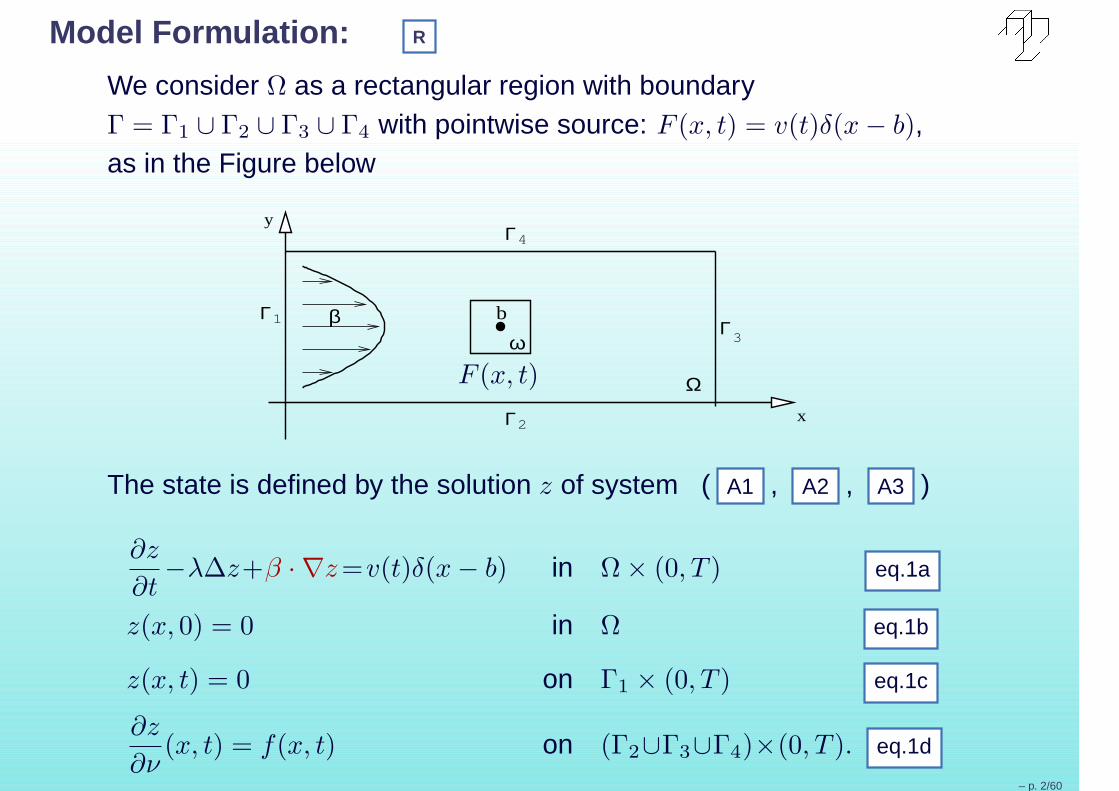
We consider Ω as a rectangular region with boundaryΓ = Γ1 ∪ Γ2 ∪ Γ3 ∪ Γ4 with pointwise source: F (x, t) = v(t)δ(x − b),as in the Figure below
x
yΓ
Γ
Ω
ωbβ
Γ
Γ3
1
2
4
F (x, t)
The state is defined by the solution z of system ( A1 , A2 , A3 )
∂z
∂t−λ∆z+β · ∇z=v(t)δ(x − b) in Ω × (0, T ) eq.1a
z(x, 0) = 0 in Ω eq.1b
z(x, t) = 0 on Γ1 × (0, T ) eq.1c
∂z
∂ν(x, t) = f(x, t) on (Γ2∪Γ3∪Γ4)×(0, T ). eq.1d
– p. 2/60
• z(x, t) stands for the pollutant’s concentration at (x, t) ∈ Ω × [0, T ].
• λ > 0 is the diffusion coefficient.
• β is the velocity vector with βi ∈ C1(Ω).
• v(t) is the pointwise control.
• δ(x − b) is the Dirac mass at b, where b determines the point ofpollution entrance.
• T > 0 is given.
• Condition (1)b states that in the initial time the pollution is null.
• Condition (1)c states that in any time t ∈ (0, T ) in boundary Γ1
there is no pollution.
• Condition (1)d represents the diffusive flow of pollution throughboundaries Γ2 ∪ Γ3 ∪ Γ4 by the function f , where f is given inL2
(
0, T ; H1
2 (Γ2 ∪ Γ3 ∪ Γ4))
.
• ∂z/∂ν = ∇z · ν, where ν is the normal unitary vector exterior to Ω.
– p. 3/60
Cost functional
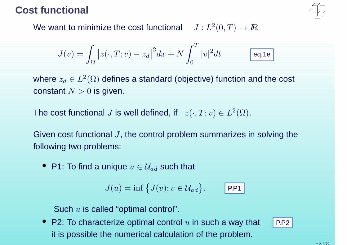
We want to minimize the cost functional J : L2(0, T ) → IR
J(v) =
∫
Ω
∣
∣z(·, T ; v) − zd
∣
∣
2dx + N
∫ T
0
|v|2dt eq.1e
where zd ∈ L2(Ω) defines a standard (objective) function and the costconstant N > 0 is given.
The cost functional J is well defined, if z(·, T ; v) ∈ L2(Ω).
Given cost functional J , the control problem summarizes in solving thefollowing two problems:
• P1: To find a unique u ∈ Uad such that
J(u) = inf
J(v); v ∈ Uad
. P.P1
Such u is called “optimal control”.• P2: To characterize optimal control u in such a way that P.P2
it is possible the numerical calculation of the problem.– p. 4/60
Application
We study the case of the contamination of a river or lagoon by mercury(Hg).
In this case, by the Brazilian Legislation, the acceptable level zd ofpollution of mercury (Hg) in
• drinking water is given by: zd = 2 × 10⁻⁶mg/l,
• effluent is given by: zd = 2 × 10⁻³mg/l.
We will consider in 1a : Water without movement: β = 0.
Water in movement: β 6= 0.
Our problem consists of determining ways (through the controls) insuch a way to minimize the effect caused by the debris of pollutant.
– p. 5/60
Objective: To solve the problems P1 and P2.
Stages to follow :
• To show that the state system given by 1b admits a uniquesolution.
• To show the existence of a unique optimal control u that minimizesthe functional J on a set of admissible functions Uad. Being themost important aspect of the mathematical point of view.
• To get a characterization for the optimal control u and from thischaracterization the optimality system that allows the numericalcalculation of the problem. Being the most important aspect of thenumerical point of view.
• To get a numerical solution of the problem by using stabilizedmethod SUPG of semidiscrete finite elements.
• To plot the numerical solution.
– p. 6/60
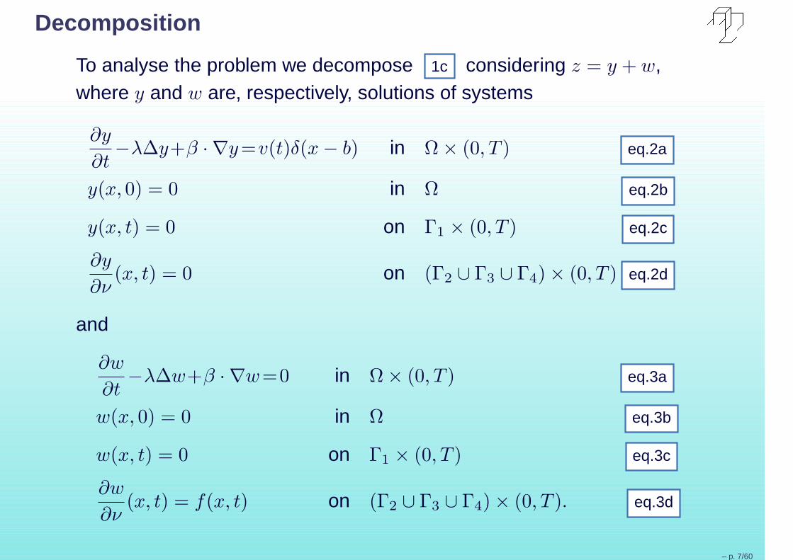
Decomposition
To analyse the problem we decompose 1c considering z = y + w,where y and w are, respectively, solutions of systems
∂y
∂t−λ∆y+β · ∇y=v(t)δ(x − b) in Ω × (0, T ) eq.2a
y(x, 0) = 0 in Ω eq.2b
y(x, t) = 0 on Γ1 × (0, T ) eq.2c
∂y
∂ν(x, t) = 0 on (Γ2 ∪ Γ3 ∪ Γ4) × (0, T ) eq.2d
and
∂w
∂t−λ∆w+β · ∇w=0 in Ω × (0, T ) eq.3a
w(x, 0) = 0 in Ω eq.3b
w(x, t) = 0 on Γ1 × (0, T ) eq.3c
∂w
∂ν(x, t) = f(x, t) on (Γ2 ∪ Γ3 ∪ Γ4) × (0, T ). eq.3d
– p. 7/60
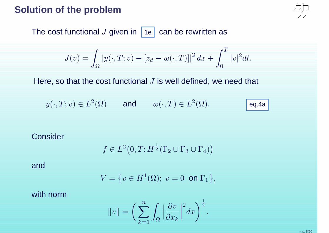
Solution of the problem
The cost functional J given in 1e can be rewritten as
J(v) =
∫
Ω
|y(·, T ; v) − [zd − w(·, T )]|2dx +
∫ T
0
|v|2dt.
Here, so that the cost functional J is well defined, we need that
y(·, T ; v) ∈ L2(Ω) and w(·, T ) ∈ L2(Ω). eq.4a
Consider
f ∈ L2(
0, T ; H1
2 (Γ2 ∪ Γ3 ∪ Γ4))
and
V =
v ∈ H1(Ω); v = 0 on Γ1
,
with norm
‖v‖ =
( n∑
k=1
∫
Ω
∣
∣
∣
∂v
∂xk
∣
∣
∣
2
dx
)1
2
.
– p. 8/60
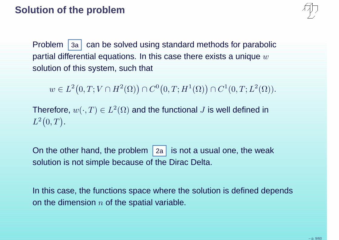
Solution of the problem
Problem 3a can be solved using standard methods for parabolicpartial differential equations. In this case there exists a unique w
solution of this system, such that
w ∈ L2(
0, T ; V ∩ H2(Ω))
∩ C0(
0, T ; H1(Ω))
∩ C1(0, T ; L2(Ω)).
Therefore, w(·, T ) ∈ L2(Ω) and the functional J is well defined inL2
(
0, T)
.
On the other hand, the problem 2a is not a usual one, the weaksolution is not simple because of the Dirac Delta.
In this case, the functions space where the solution is defined dependson the dimension n of the spatial variable.
– p. 9/60
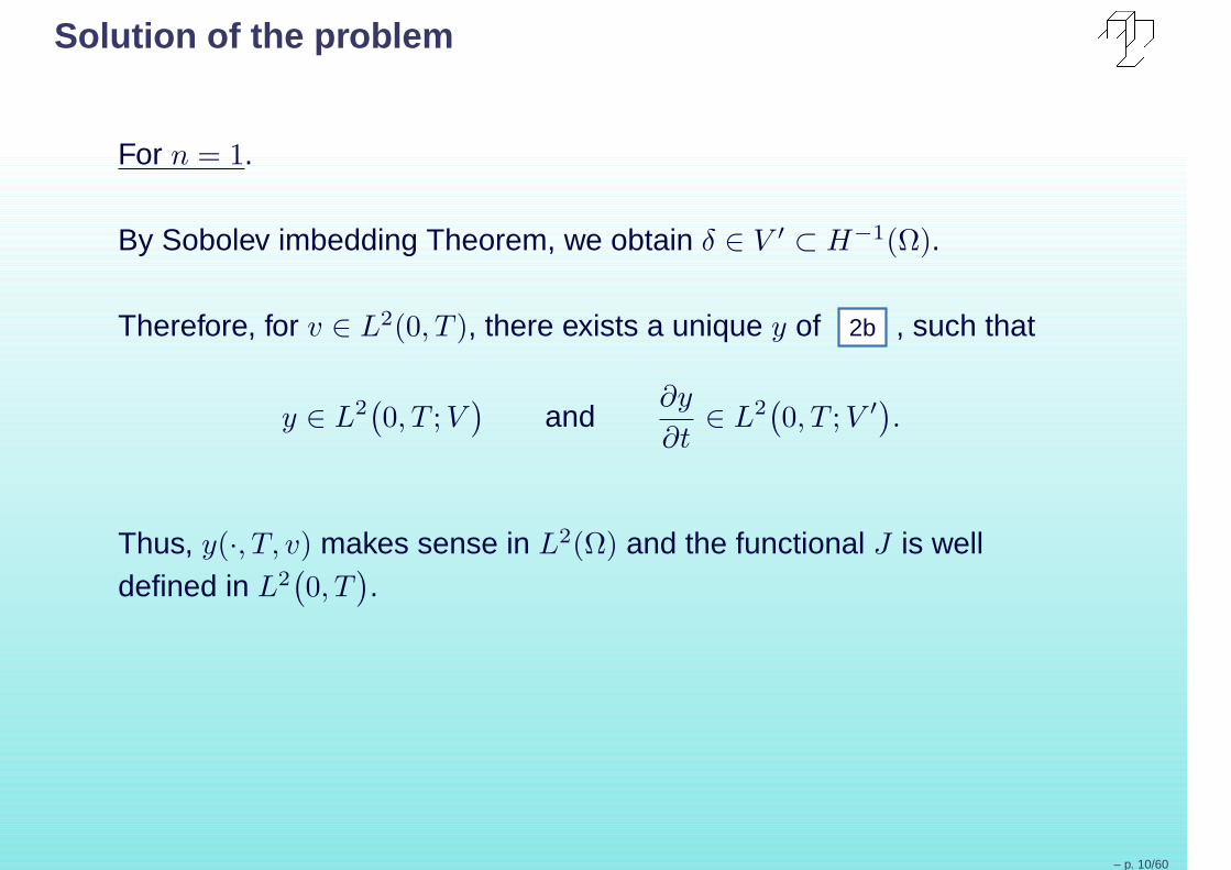
Solution of the problem
For n = 1.
By Sobolev imbedding Theorem, we obtain δ ∈ V ′ ⊂ H−1(Ω).
Therefore, for v ∈ L2(0, T ), there exists a unique y of 2b , such that
y ∈ L2(
0, T ; V)
and∂y
∂t∈ L2
(
0, T ; V ′)
.
Thus, y(·, T, v) makes sense in L2(Ω) and the functional J is welldefined in L2
(
0, T)
.
– p. 10/60
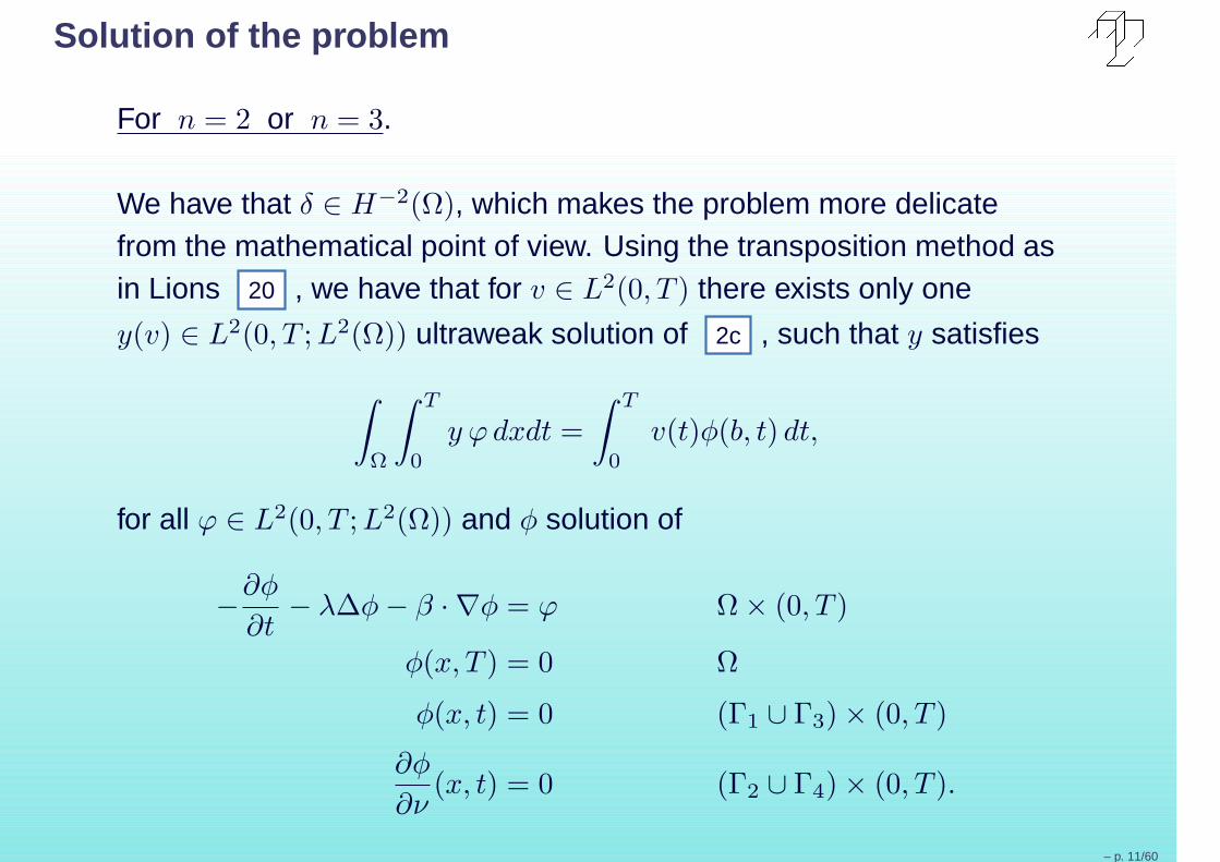
Solution of the problem
For n = 2 or n = 3.
We have that δ ∈ H−2(Ω), which makes the problem more delicatefrom the mathematical point of view. Using the transposition method asin Lions 20 , we have that for v ∈ L2(0, T ) there exists only one
y(v) ∈ L2(0, T ; L2(Ω)) ultraweak solution of 2c , such that y satisfies
∫
Ω
∫ T
0
y ϕ dxdt =
∫ T
0
v(t)φ(b, t) dt,
for all ϕ ∈ L2(0, T ; L2(Ω)) and φ solution of
−∂φ
∂t− λ∆φ − β · ∇φ = ϕ Ω × (0, T )
φ(x, T ) = 0 Ω
φ(x, t) = 0 (Γ1 ∪ Γ3) × (0, T )
∂φ
∂ν(x, t) = 0 (Γ2 ∪ Γ4) × (0, T ).
– p. 11/60
Solution of the problem
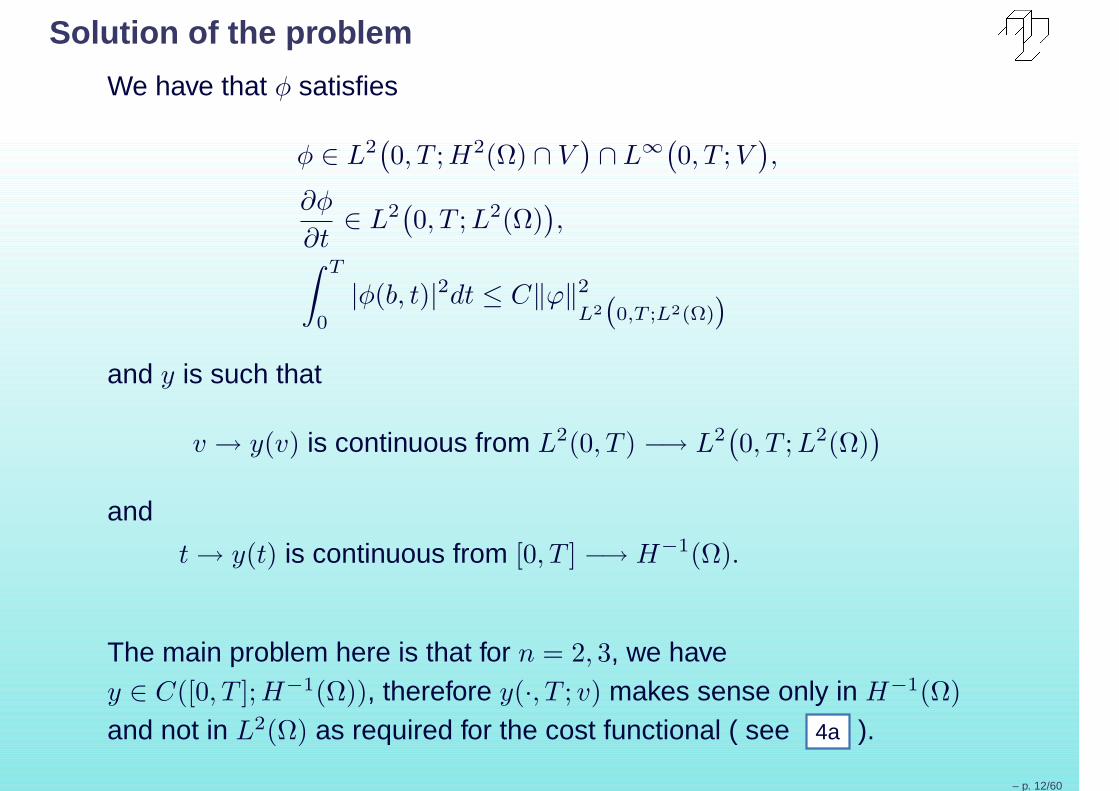
We have that φ satisfies
φ ∈ L2(
0, T ; H2(Ω) ∩ V)
∩ L∞(
0, T ; V)
,
∂φ
∂t∈ L2
(
0, T ; L2(Ω))
,
∫ T
0
|φ(b, t)|2dt ≤ C‖ϕ‖2
L2
(
0,T ;L2(Ω))
and y is such that
v → y(v) is continuous from L2(0, T ) −→ L2(
0, T ; L2(Ω))
and
t → y(t) is continuous from [0, T ] −→ H−1(Ω).
The main problem here is that for n = 2, 3, we havey ∈ C([0, T ];H−1(Ω)), therefore y(·, T ; v) makes sense only in H−1(Ω)
and not in L2(Ω) as required for the cost functional ( see 4a ).
– p. 12/60
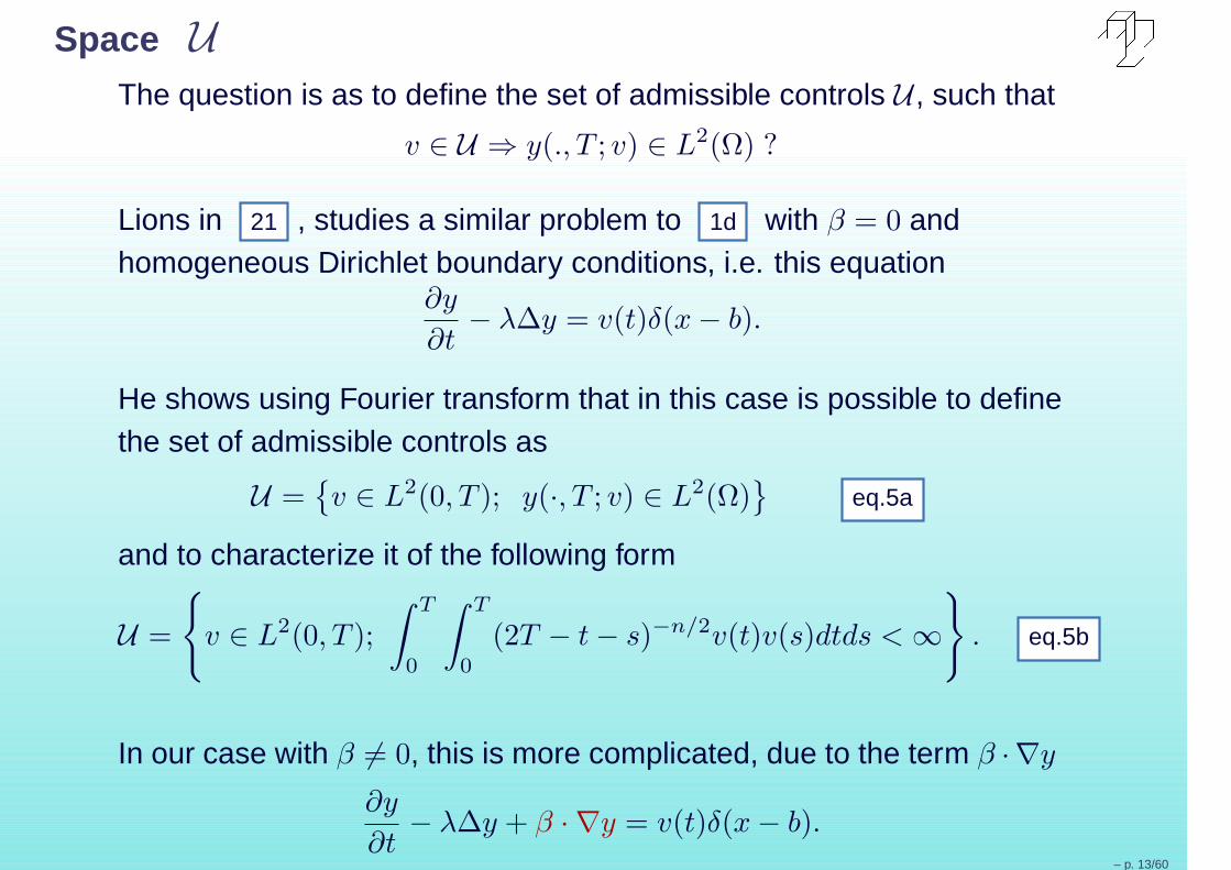
Space UThe question is as to define the set of admissible controls U , such that
v ∈ U ⇒ y(., T ; v) ∈ L2(Ω) ?
Lions in 21 , studies a similar problem to 1d with β = 0 andhomogeneous Dirichlet boundary conditions, i.e. this equation
∂y
∂t− λ∆y = v(t)δ(x − b).
He shows using Fourier transform that in this case is possible to definethe set of admissible controls as
U =
v ∈ L2(0, T ); y(·, T ; v) ∈ L2(Ω)
eq.5a
and to characterize it of the following form
U =
v ∈ L2(0, T );
∫ T
0
∫ T
0
(2T − t − s)−n/2v(t)v(s)dtds < ∞
. eq.5b
In our case with β 6= 0, this is more complicated, due to the term β · ∇y
∂y
∂t− λ∆y + β · ∇y = v(t)δ(x − b).
– p. 13/60
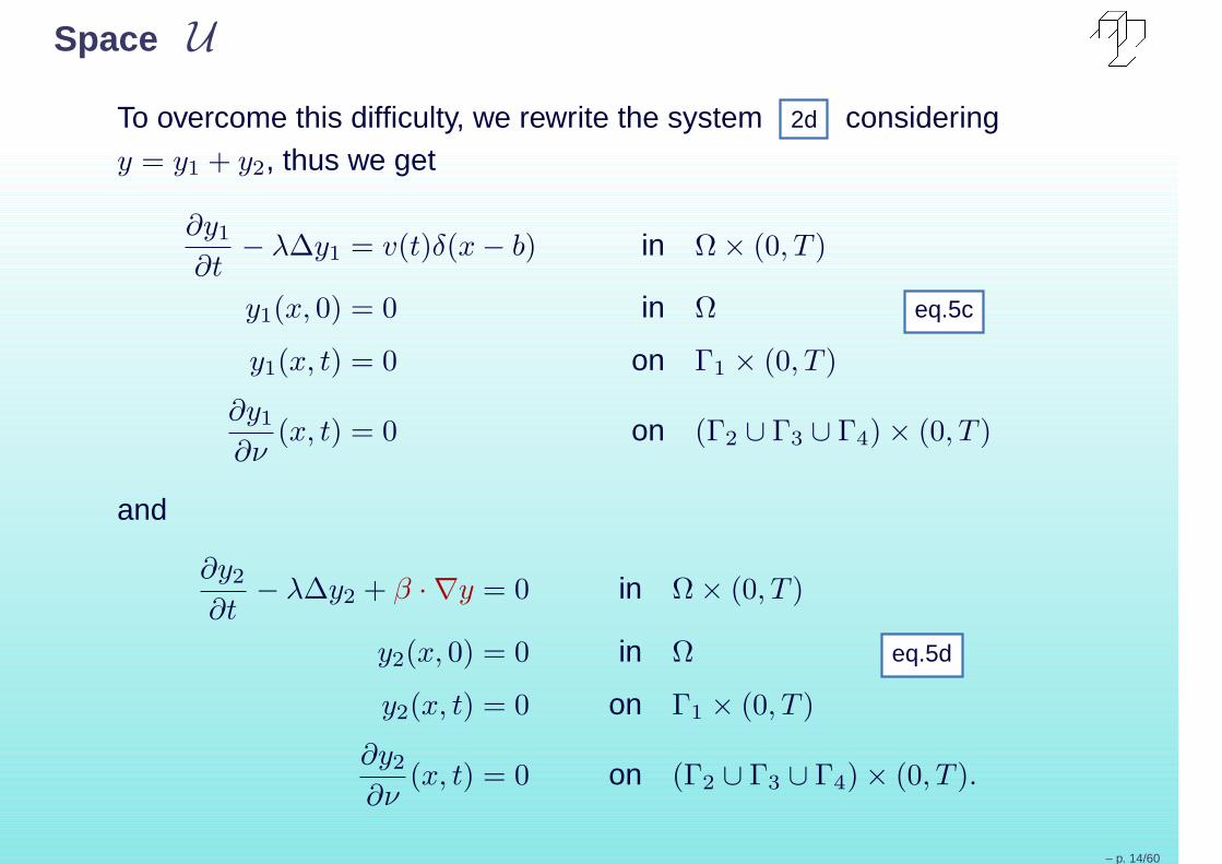
Space U
To overcome this difficulty, we rewrite the system 2d consideringy = y1 + y2, thus we get
∂y1
∂t− λ∆y1 = v(t)δ(x − b) in Ω × (0, T )
y1(x, 0) = 0 in Ω eq.5c
y1(x, t) = 0 on Γ1 × (0, T )
∂y1
∂ν(x, t) = 0 on (Γ2 ∪ Γ3 ∪ Γ4) × (0, T )
and
∂y2
∂t− λ∆y2 + β · ∇y = 0 in Ω × (0, T )
y2(x, 0) = 0 in Ω eq.5d
y2(x, t) = 0 on Γ1 × (0, T )
∂y2
∂ν(x, t) = 0 on (Γ2 ∪ Γ3 ∪ Γ4) × (0, T ).
– p. 14/60

Space U
In the problem 5c , we use the Lions’ result. In problem 5d , of thetheory of parabolic equations, we have thaty2 ∈ L2
(
0, T ; V)
∩ C0(
[0, T ];L2(Ω))
and y2t ∈ L2(
0, T ; H−1(Ω))
.
Therefore, y ∈ C0(0, T ; L2(Ω)) and in particular, y(·, T ) ∈ L2(Ω).
According to this, we can define the space U of admissible controlsand its characterization of the same form that Lions as in 5a and
5b respectively. Which with the norms
‖v‖2U =
∫ T
0
|v|2dt +
∫
Ω
|y(·, T ; v)|2dx
‖|v‖|2U =
∫ T
0
|v|2dt +
∫ T
0
∫ T
0
(2T − t − s)−n/2v(t)v(s)dtds
respectively, are Hilbert spaces.
The norms given above are equivalents.
– p. 15/60
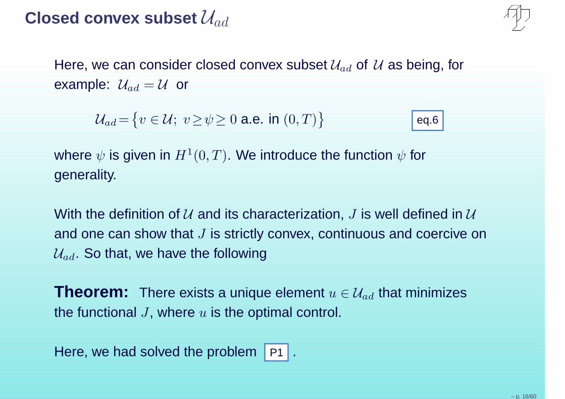
Closed convex subset Uad
Here, we can consider closed convex subset Uad of U as being, forexample: Uad = U or
Uad =
v ∈ U ; v≥ψ≥ 0 a.e. in (0, T )
eq.6
where ψ is given in H1(0, T ). We introduce the function ψ forgenerality.
With the definition of U and its characterization, J is well defined in U
and one can show that J is strictly convex, continuous and coercive onUad. So that, we have the following
Theorem: There exists a unique element u ∈ Uad that minimizesthe functional J , where u is the optimal control.
Here, we had solved the problem P1 .
– p. 16/60
Properties of the Space U : (see 22 )
• U does not depend on Ω.
• U does not depend on the boundary conditions.
• C∞0 (0, T ) ⊂ U .
• L20(0, T )=
v ∈ L2(0, T ); v ≡ 0 in (T − ǫ, T ), ǫ ≥ 0
is dense in U ,by the regularizing effect.
Space D(0, T ) is dense in U . Therefore, if U ′ denotes the dual spaceof U , then
D(0, T ) ⊂ U ⊂ L2(0, T ) ⊂ U ′ ⊂ D′(0, T ).
– p. 17/60
Characterization of the Optimal Control
Theorem: Through the Gâteaux derivative of J , the optimal controlu is characterized, ∀ v ∈ Uad and u ∈ Uad, by
∫
Ω
y(·, T ; u) − [zd − w(·, T )]y(·, T ; v−u)dx+N
∫ T
0
u(v−u)dt ≥ 0. eq.7
This estimate is not appropriate to numerical analysis, because doesnot describe u in explicit form. To get a more adequatedcharacterization of u, we introduce the adjoint operator of y.
−∂q
∂t− λ∆q − β · ∇q = 0 in Ω × (0, T )
q(x, T ; u) = y(x, T ; u) −[
zd − w(x, T )]
in Ω eq.8
q(x, t) = 0 on Γ1 × (0, T )
λ∂q(x, t)
∂ν+ q(x, t)(β · ν) = 0 on (Γ2 ∪ Γ3 ∪ Γ4) × (0, T ),
where q ∈ L2(
0, T ; V)
∩ C0([0, T ];L2(Ω)) and satisfiesq ∈ C∞([0, T ) × Ω); therefore, we can define q(b, t) for t < T .
– p. 18/60
Better characterization
Using adjoint system 8 we arrive at a similar Lions’ 23 result.
Theorem: One has q(b, t) ∈ U ′ and condition 7 is equivalent to
∫ T
0
(
q(b, t)+ Nu)
(v − u)dt ≥ 0, ∀ v ∈ Uad, u ∈ Uad,
where the integral above denotes duality between U ′ and U .
– p. 19/60
Explicit form of u
With this better characterization, we get u in explicit form for someconvex closed Uad. For example:
• If Uad = U , the optimal control is given by
u = −1
Nq(b, t).
• If Uad = v ∈ U ; v ≥ ψ ≥ 0 a.e. in (0, T ), with ψ given inH1(0, T ), we obtain
u = ψ +
(
1
Nq(b, t) + ψ
)−
, as ψ 6= 0
and
u =
(
1
Nq(b, t)
)−
, as ψ ≡ 0,
where f−=max0,−f. For applications, the controls must be positive,therefore we consider the closed convex subset Uad given by 6 .
With the explicit form of u, we already solved the problem P2 .– p. 20/60
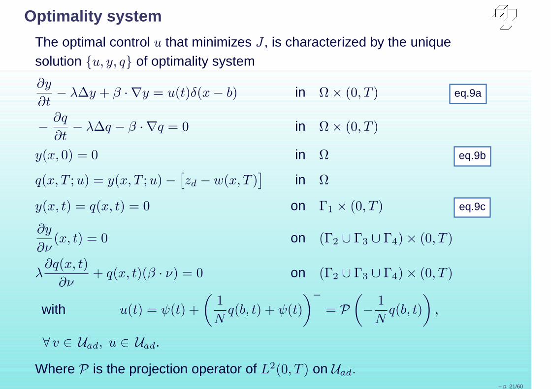
Optimality system
The optimal control u that minimizes J , is characterized by the uniquesolution u, y, q of optimality system
∂y
∂t− λ∆y + β · ∇y = u(t)δ(x − b) in Ω × (0, T ) eq.9a
−∂q
∂t− λ∆q − β · ∇q = 0 in Ω × (0, T )
y(x, 0) = 0 in Ω eq.9b
q(x, T ; u) = y(x, T ; u) −[
zd − w(x, T )]
in Ω
y(x, t) = q(x, t) = 0 on Γ1 × (0, T ) eq.9c
∂y
∂ν(x, t) = 0 on (Γ2 ∪ Γ3 ∪ Γ4) × (0, T )
λ∂q(x, t)
∂ν+ q(x, t)(β · ν) = 0 on (Γ2 ∪ Γ3 ∪ Γ4) × (0, T )
with u(t) = ψ(t) +
(
1
Nq(b, t) + ψ(t)
)−
= P
(
−1
Nq(b, t)
)
,
∀ v ∈ Uad, u ∈ Uad.
Where P is the projection operator of L2(0, T ) on Uad.– p. 21/60
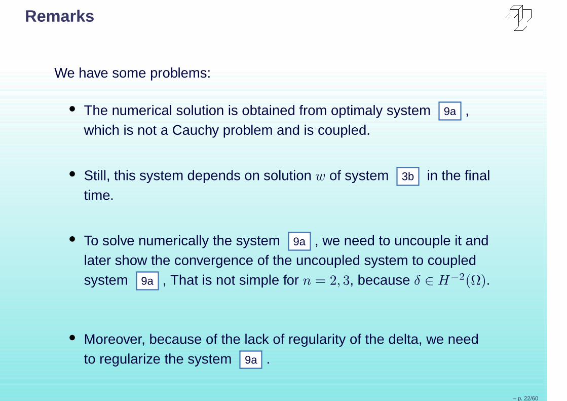
Remarks
We have some problems:
• The numerical solution is obtained from optimaly system 9a ,which is not a Cauchy problem and is coupled.
• Still, this system depends on solution w of system 3b in the finaltime.
• To solve numerically the system 9a , we need to uncouple it andlater show the convergence of the uncoupled system to coupledsystem 9a , That is not simple for n = 2, 3, because δ ∈ H−2(Ω).
• Moreover, because of the lack of regularity of the delta, we needto regularize the system 9a .
– p. 22/60
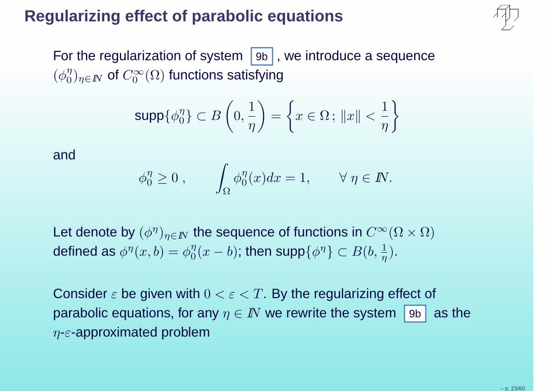
Regularizing effect of parabolic equations
For the regularization of system 9b , we introduce a sequence(φη
0)η∈IN of C∞0 (Ω) functions satisfying
suppφη0 ⊂ B
(
0,1
η
)
=
x ∈ Ω ; ‖x‖ <1
η
and
φη0 ≥ 0 ,
∫
Ω
φη0(x)dx = 1, ∀ η ∈ IN.
Let denote by (φη)η∈IN the sequence of functions in C∞(Ω × Ω)
defined as φη(x, b) = φη0(x − b); then suppφη ⊂ B(b, 1
η ).
Consider ε be given with 0 < ε < T . By the regularizing effect ofparabolic equations, for any η ∈ IN we rewrite the system 9b as theη-ε-approximated problem
– p. 23/60
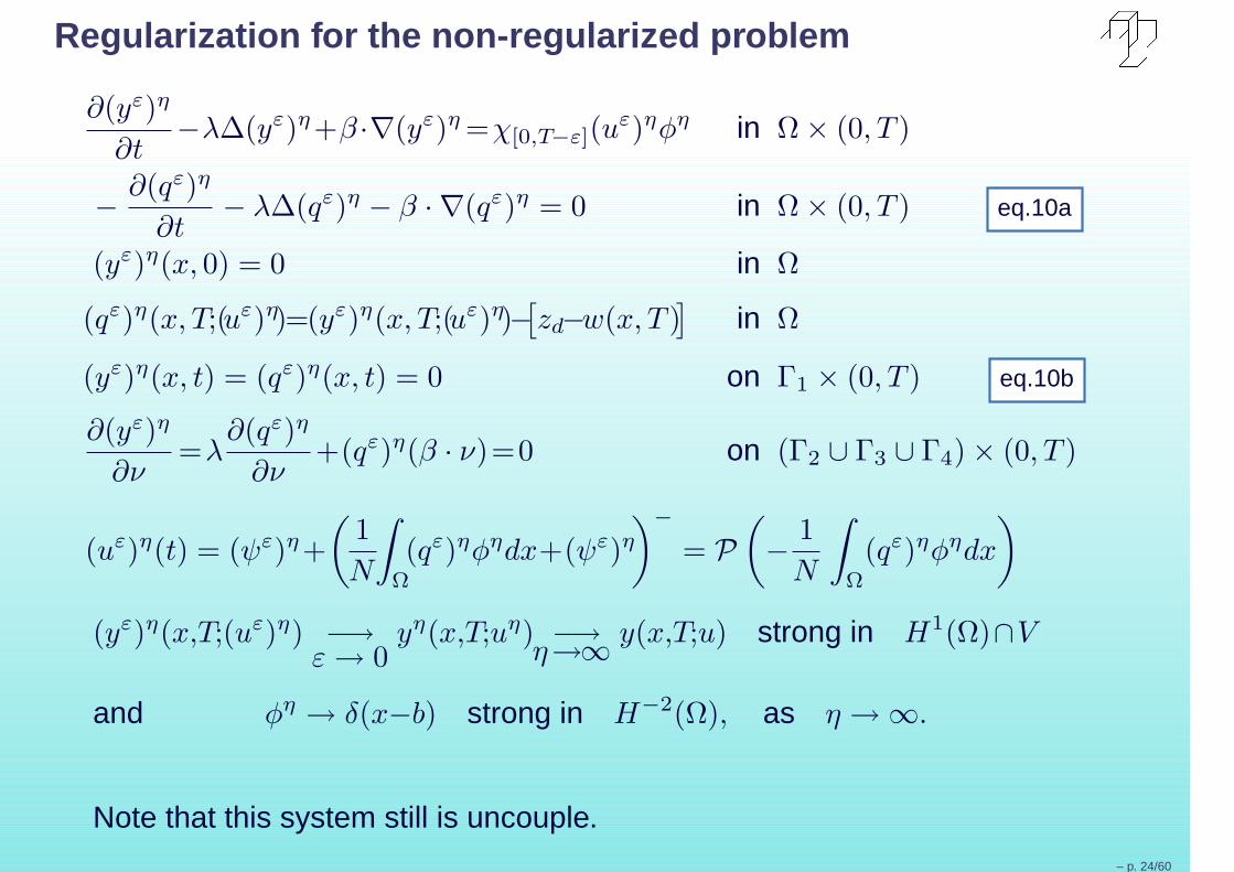
Regularization for the non-regularized problem
∂(yε)η
∂t−λ∆(yε)η+β ·∇(yε)η =χ[0,T−ε](u
ε)ηφη in Ω × (0, T )
−∂(qε)η
∂t− λ∆(qε)η − β · ∇(qε)η = 0 in Ω × (0, T ) eq.10a
(yε)η(x, 0) = 0 in Ω
(qε)η(x, T;(uε)η)=(yε)η(x, T;(uε)η)−[
zd−w(x, T )]
in Ω
(yε)η(x, t) = (qε)η(x, t) = 0 on Γ1 × (0, T ) eq.10b
∂(yε)η
∂ν=λ
∂(qε)η
∂ν+(qε)η(β · ν)=0 on (Γ2 ∪ Γ3 ∪ Γ4) × (0, T )
(uε)η(t) = (ψε)η+
(
1
N
∫
Ω
(qε)ηφηdx+(ψε)η
)−
= P
(
−1
N
∫
Ω
(qε)ηφηdx
)
(yε)η(x,T;(uε)η) −→ε → 0
yη(x,T;uη) −→η→∞
y(x,T;u) strong in H1(Ω)∩V
and φη → δ(x−b) strong in H−2(Ω), as η → ∞.
Note that this system still is uncouple.– p. 24/60
Convergence of the non-regularized problem
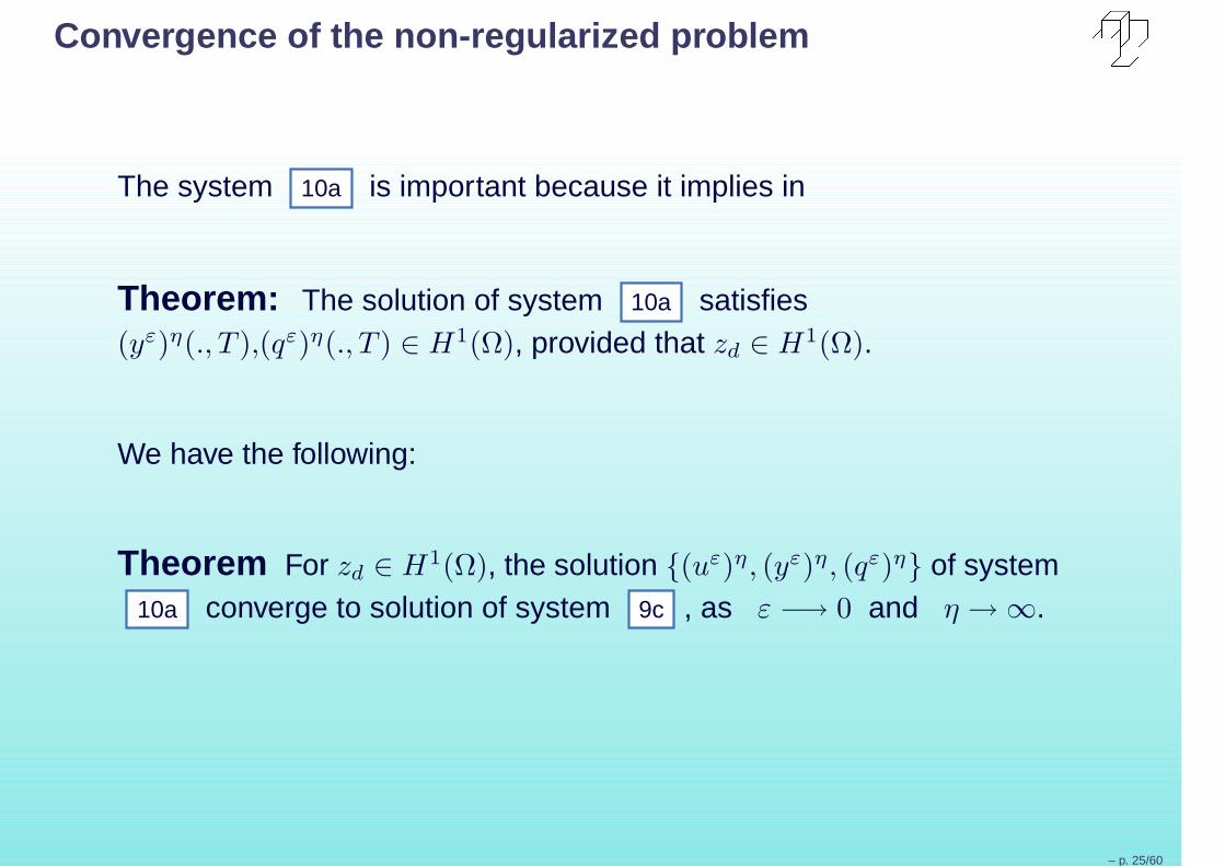
The system 10a is important because it implies in
Theorem: The solution of system 10a satisfies(yε)η(., T ),(qε)η(., T ) ∈ H1(Ω), provided that zd ∈ H1(Ω).
We have the following:
Theorem For zd ∈ H1(Ω), the solution (uε)η, (yε)η, (qε)η of system10a converge to solution of system 9c , as ε −→ 0 and η → ∞.
– p. 25/60
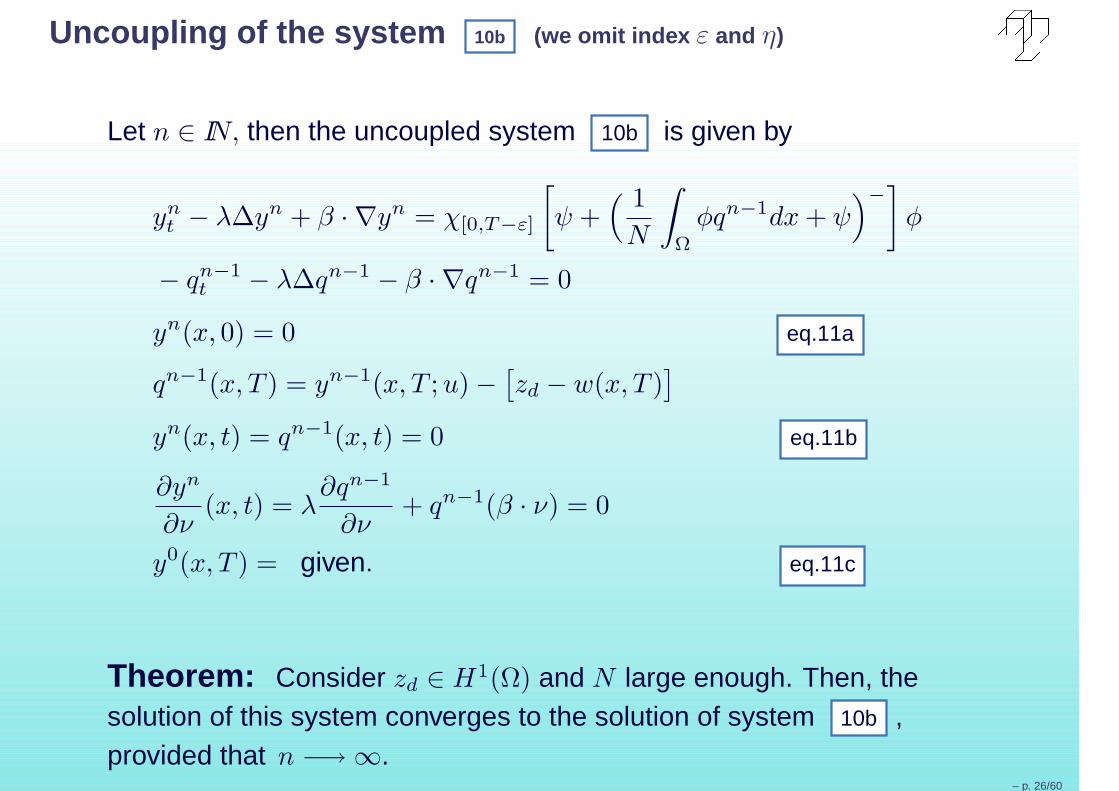
Uncoupling of the system 10b (we omit index ε and η)
Let n ∈ IN, then the uncoupled system 10b is given by
ynt − λ∆yn + β · ∇yn = χ[0,T−ε]
[
ψ +( 1
N
∫
Ω
φqn−1dx + ψ)−
]
φ
− qn−1t − λ∆qn−1 − β · ∇qn−1 = 0
yn(x, 0) = 0 eq.11a
qn−1(x, T ) = yn−1(x, T ; u) −[
zd − w(x, T )]
yn(x, t) = qn−1(x, t) = 0 eq.11b
∂yn
∂ν(x, t) = λ
∂qn−1
∂ν+ qn−1(β · ν) = 0
y0(x, T ) = given. eq.11c
Theorem: Consider zd ∈ H1(Ω) and N large enough. Then, thesolution of this system converges to the solution of system 10b ,provided that n −→ ∞.
– p. 26/60
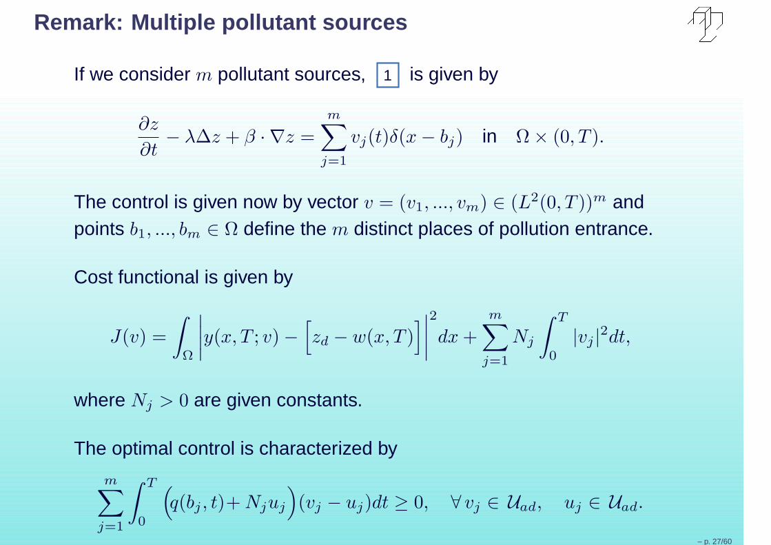
Remark: Multiple pollutant sources
If we consider m pollutant sources, 1 is given by
∂z
∂t− λ∆z + β · ∇z =
m∑
j=1
vj(t)δ(x − bj) in Ω × (0, T ).
The control is given now by vector v = (v1, ..., vm) ∈ (L2(0, T ))m andpoints b1, ..., bm ∈ Ω define the m distinct places of pollution entrance.
Cost functional is given by
J(v) =
∫
Ω
∣
∣
∣
∣
y(x, T ; v) −[
zd − w(x, T )]
∣
∣
∣
∣
2
dx +
m∑
j=1
Nj
∫ T
0
|vj |2dt,
where Nj > 0 are given constants.
The optimal control is characterized by
m∑
j=1
∫ T
0
(
q(bj , t)+ Njuj
)
(vj − uj)dt ≥ 0, ∀ vj ∈ Uad, uj ∈ Uad.
– p. 27/60
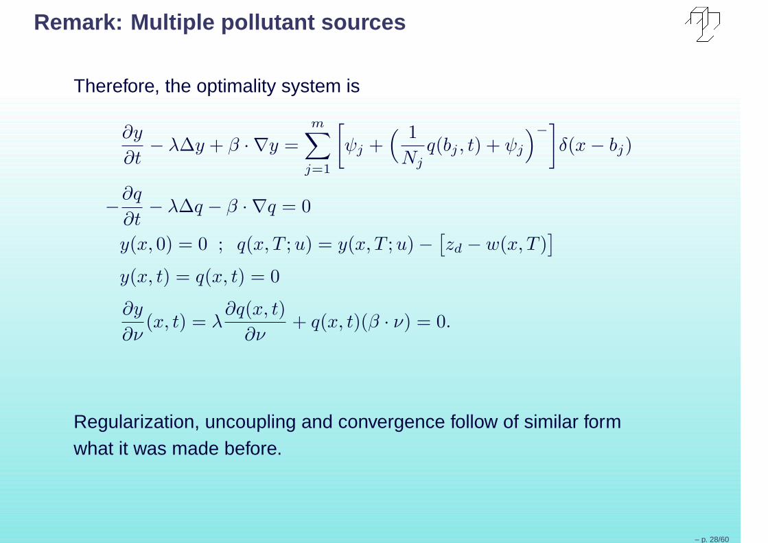
Remark: Multiple pollutant sources
Therefore, the optimality system is
∂y
∂t− λ∆y + β · ∇y =
m∑
j=1
[
ψj +( 1
Njq(bj , t) + ψj
)−]
δ(x − bj)
−∂q
∂t− λ∆q − β · ∇q = 0
y(x, 0) = 0 ; q(x, T ; u) = y(x, T ; u) −[
zd − w(x, T )]
y(x, t) = q(x, t) = 0
∂y
∂ν(x, t) = λ
∂q(x, t)
∂ν+ q(x, t)(β · ν) = 0.
Regularization, uncoupling and convergence follow of similar formwhat it was made before.
– p. 28/60
Remark: Varying point x = b of pollutant entrance
Varying point x = b of pollutant entrance, 2 not change, and for eachpoint b, among optimal controls u (that depend on point b), exists onlyone optimal control ub ∈ Uad, such that
J(
ub
)
= inf
J(
u)
; u ∈ Uad
.
This means that in Ω, apart from optimal control, there exists only onepoint bo (called strategic point or optimal point) where pollution is evenless harmful to the environment.
– p. 29/60
The numerical solution of 11a
• So that the numerical problem represents a practical situation andmakes physical sense, we take f = 0 in boundaries Γ2 ∪ Γ3 ∪ Γ4
3 . Thus, in 3c , w ≡ 0.
• First, we analyse cases of only one pollutant source and we varythe place of pollution entrance.
• Then, we analyse cases of multiple pollutant sources.
• In all the cases we consider either water without movement orwith movement.
• We use a combination of spatial discretization by stabilizedsemidiscrete finite element method and time discretization byEuler implicit method of finite differences, as in 24 .
– p. 30/60
The numerical solution of 11b
• Acceptable level zd of mercury (Hg) in drinking water iszd = 2 × 10⁻⁶sen(πx/L) sen(πy/L) mg/cm3 (see 25 - 26 ).
• Diffusion coefficient of Hg is λ = 6 × 10⁻⁶ cm2/s.
• Velocity field β = 10−4(
1 −((
y − (L/2))
/(L/2))2
, 0)
cm/s.
• Cost constant N = 15 × 104.
• Tinal time T = 8640000 s.
• We use implemented code in Fortran 90 and graphics arepresented in Maple.
• Without loss of generality, we consider ψ ≡ 0 in 11b .
– p. 31/60
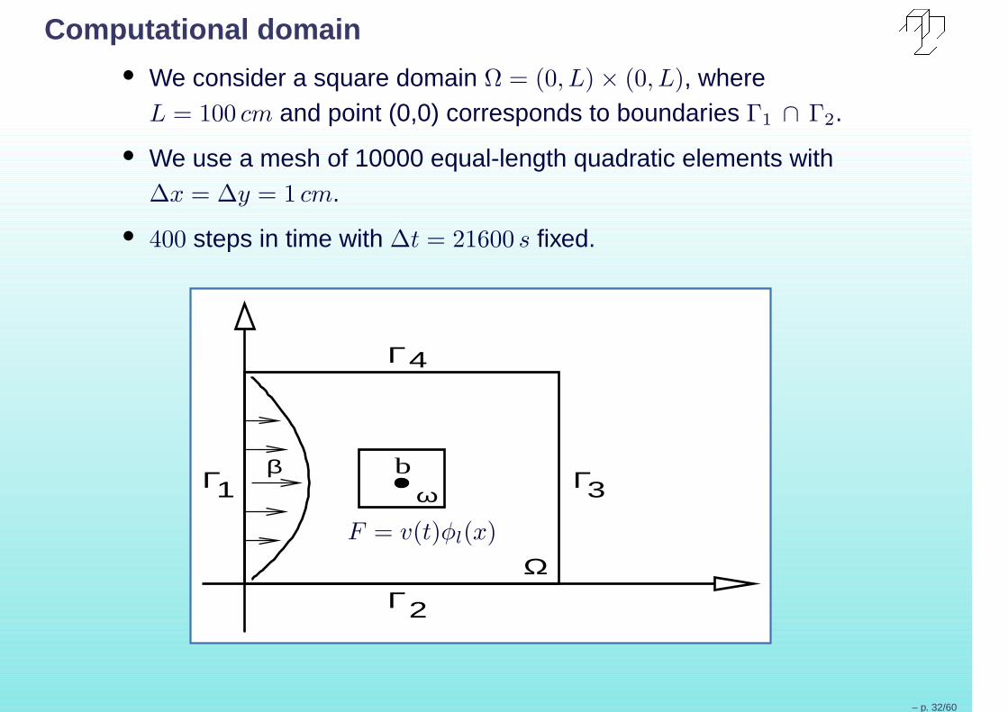
Computational domain• We consider a square domain Ω = (0, L) × (0, L), where
L = 100 cm and point (0,0) corresponds to boundaries Γ1 ∩ Γ2.
• We use a mesh of 10000 equal-length quadratic elements with∆x = ∆y = 1 cm.
• 400 steps in time with ∆t = 21600 s fixed.
Γ1 Γ3
Γ4
Γ2
Ω
β bω
F = v(t)φl(x)
– p. 32/60
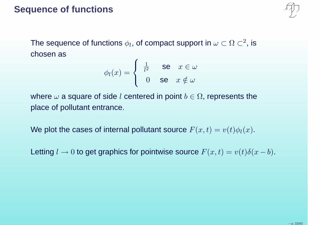
Sequence of functions
The sequence of functions φl, of compact support in ω ⊂ Ω ⊂2, ischosen as
φl(x) =
1l2 se x ∈ ω
0 se x /∈ ω
where ω a square of side l centered in point b ∈ Ω, represents theplace of pollutant entrance.
We plot the cases of internal pollutant source F (x, t) = v(t)φl(x).
Letting l → 0 to get graphics for pointwise source F (x, t) = v(t)δ(x− b).
– p. 33/60
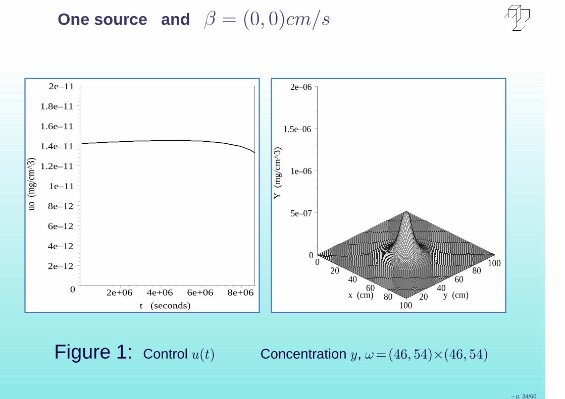
One source and β = (0, 0)cm/s
0
2e–12
4e–12
6e–12
8e–12
1e–11
1.2e–11
1.4e–11
1.6e–11
1.8e–11
2e–11
u
o (m
g/cm
^3)
2e+06 4e+06 6e+06 8e+06
t (seconds)
020
4060
80100
x (cm) 2040
6080
100
y (cm)
0
5e–07
1e–06
1.5e–06
2e–06
Y (m
g/c
m^3
)
Figure 1: Control u(t) Concentration y, ω=(46, 54)×(46, 54)
– p. 34/60

One source and β = (0, 0)cm/s
0
2e–12
4e–12
6e–12
8e–12
1e–11
1.2e–11
1.4e–11
1.6e–11
1.8e–11
2e–11
u
o (m
g/cm
^3)
2e+06 4e+06 6e+06 8e+06
t (seconds)
020
4060
80100
x (cm) 2040
6080
100
y (cm)
0
5e–07
1e–06
1.5e–06
2e–06
Y (m
g/c
m^3
)
Figure 2: Control u(t) Concentration y, ω=(49, 51)×(49, 51)
– p. 35/60
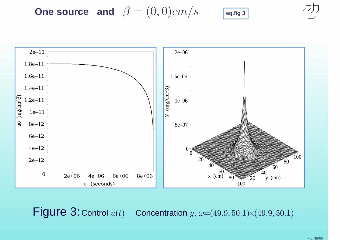
One source and β = (0, 0)cm/s eq.fig 3
0
2e–12
4e–12
6e–12
8e–12
1e–11
1.2e–11
1.4e–11
1.6e–11
1.8e–11
2e–11
u
o (m
g/cm
^3)
2e+06 4e+06 6e+06 8e+06
t (seconds)
020
4060
80100
x (cm) 2040
6080
100
y (cm)
0
5e–07
1e–06
1.5e–06
2e–06
Y (m
g/c
m^3
)
Figure 3:Control u(t) Concentration y, ω=(49.9, 50.1)×(49.9, 50.1)
– p. 36/60
Comments:
In this case (water without movement), we note that initially we canpour certain amount of pollution, such that in elapsing time, thisamount diminishes so that the pollution concentration in the final timey(x, T ; u(T )) does not exceed the allowed value zd.
We observe that the control is decreasing and, through the graphics ofthe concentration, we see that as the square region ω diminishes, thatis, as l → 0, we move from located source profile F (x, t) = u(t)φl(x) topointwise source profile F (x, t) = u(t)δ(x−b), characterizing thenumerical convergence of the sequence φl(x) for δ(x−b).
– p. 37/60
One source and β = (0, 0)cm/s
0
2e–12
4e–12
6e–12
8e–12
1e–11
1.2e–11
1.4e–11
1.6e–11
1.8e–11
2e–11
u
o (m
g/cm
^3)
2e+06 4e+06 6e+06 8e+06
t (seconds)
020
4060
80100
x (cm) 2040
6080
100
y (cm)
0
5e–07
1e–06
1.5e–06
2e–06
Y (m
g/c
m^3
)
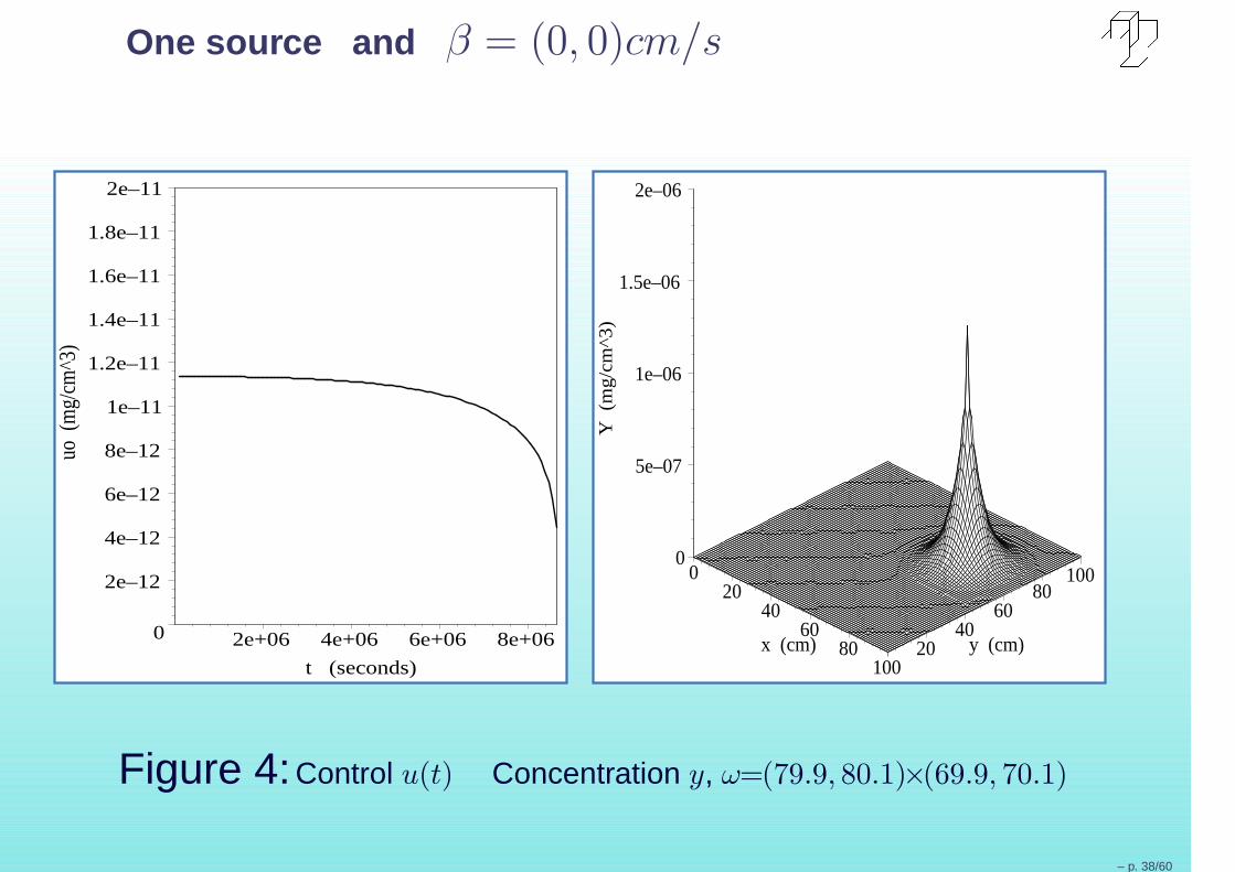
Figure 4:Control u(t) Concentration y, ω=(79.9, 80.1)×(69.9, 70.1)
– p. 38/60
One source and β = (0, 0)cm/s
0
2e–12
4e–12
6e–12
8e–12
1e–11
1.2e–11
1.4e–11
1.6e–11
1.8e–11
2e–11
u
o (m
g/cm
^3)
2e+06 4e+06 6e+06 8e+06
t (seconds)
020
4060
80100
x (cm) 2040
6080
100
y (cm)
0
5e–07
1e–06
1.5e–06
2e–06
Y (m
g/c
m^3
)
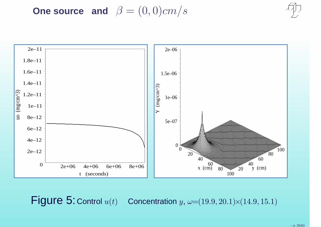
Figure 5:Control u(t) Concentration y, ω=(19.9, 20.1)×(14.9, 15.1)
– p. 39/60
Comments:Note that in graphics (3), (4) and (5), we choose the region ω ofpollution entrance, with same area 0.2 × 0.2 cm2, in different positionsin domain Ω.
We observe that the poured amount of pollution depends on thelocalization of the source.
We noted that in the central region of the domain, the pollutant hasmore freedom of spreading, then a greater amount of pollution can bepoured in this place and consequently the pollution concentration atthe final time reaches a greater index, close to zd.
Now, as the pollutant source moves from the central region, the pouredamount of pollution diminishes and therefore the pollutionconcentration also diminishes.
Here also as time passes, the amount of pollution must diminish, sothat the pollution concentration in the final time y(x, T ; u(T )) does notexceed the value of zd.
Finally, we observe that the control is also decreasing.
– p. 40/60
One source, β 6= (0, 0)cm/s (water in movement)
0
2e–12
4e–12
6e–12
8e–12
1e–11
1.2e–11
1.4e–11
1.6e–11
1.8e–11
2e–11
u
o (m
g/cm
^3)
2e+06 4e+06 6e+06 8e+06
t (seconds)
020
4060
80100
x (cm) 2040
6080
100
y (cm)
0
5e–07
1e–06
1.5e–06
2e–06
Y (m
g/c
m^3
)
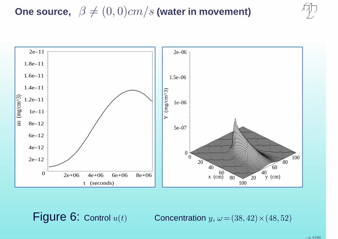
Figure 6: Control u(t) Concentration y, ω=(38, 42)×(48, 52)
– p. 41/60
One source, β 6= (0, 0)cm/s (water in movement)
eq.fig 7
0
5e–12
1e–11
1.5e–11
2e–11
u
o (m
g/cm
^3)
2e+06 4e+06 6e+06 8e+06
t (seconds)
020
4060
80100
x (cm) 2040
6080
100
y (cm)
0
5e–07
1e–06
1.5e–06
2e–06
Y
(mg
/cm
^3)
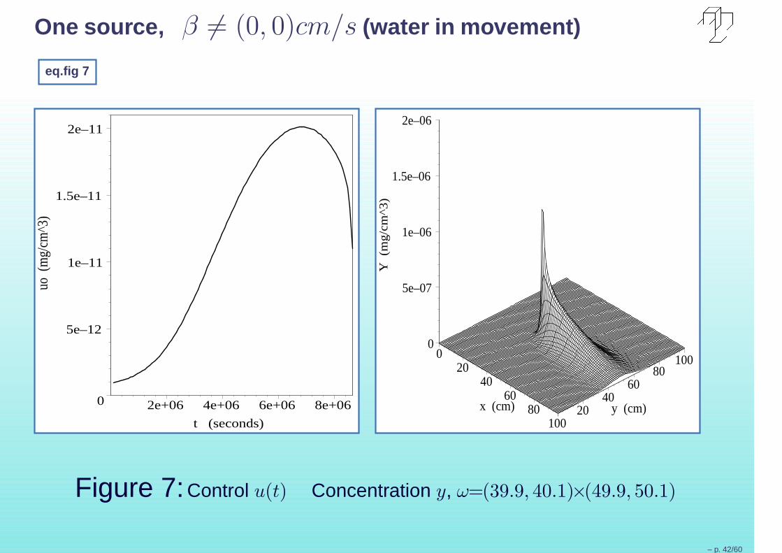
Figure 7:Control u(t) Concentration y, ω=(39.9, 40.1)×(49.9, 50.1)
– p. 42/60

Comments:
Here, we see that the amount of pollution starts being poured in adefined level, is increased and later diminished in elapsing time. Inrelations to pollution concentration, we note similar behavior to the oneof water without movement, when we diminish square region ω.
– p. 43/60
Three sources and β = (0, 0)cm/s
0
2e–12
4e–12
6e–12
8e–12
1e–11
1.2e–11
1.4e–11
1.6e–11
1.8e–11
2e–11
u
o (m
g/cm
^3)
2e+06 4e+06 6e+06 8e+06
t (seconds)
020
4060
80100
x (cm) 2040
6080
100
y (cm)
0
5e–07
1e–06
1.5e–06
2e–06
Y (m
g/c
m^3
)
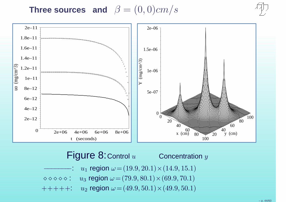
Figure 8:Control u Concentration y
−−−−−−−−: u1 region ω=(19.9, 20.1)×(14.9, 15.1)
⋄ ⋄ ⋄ ⋄ ⋄ : u3 region ω=(79.9, 80.1)×(69.9, 70.1)
+++++: u2 region ω=(49.9, 50.1)×(49.9, 50.1)
– p. 44/60
Three sources, β6=(0, 0)cm/s (water in movement)
0
2e–12
4e–12
6e–12
8e–12
1e–11
1.2e–11
1.4e–11
1.6e–11
1.8e–11
2e–11
u
o (m
g/cm
^3)
2e+06 4e+06 6e+06 8e+06
t (seconds)
020
4060
80100
x (cm) 2040
6080
100
y (cm)
0
5e–07
1e–06
1.5e–06
2e–06
Y
(mg
/cm
^3)
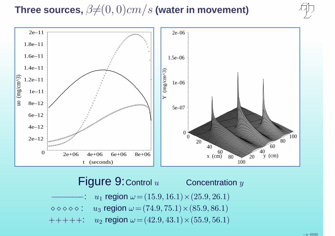
Figure 9:Control u Concentration y
−−−−−−−−: u1 region ω=(15.9, 16.1)×(25.9, 26.1)
⋄ ⋄ ⋄ ⋄ ⋄ : u3 region ω=(74.9, 75.1)×(85.9, 86.1)
+++++: u2 region ω=(42.9, 43.1)×(55.9, 56.1)
– p. 45/60
Comments:
We observe that either the control or the pollution concentrationbehave similarly to the case of only one source.
Note that in figure (8), on purpose we choose the same places ofpollution entrance of figures (3), (4) and (5).
We made repeated simulations varying the parameters of the model,and in all the cases we evidence the convergence of the method.
– p. 46/60
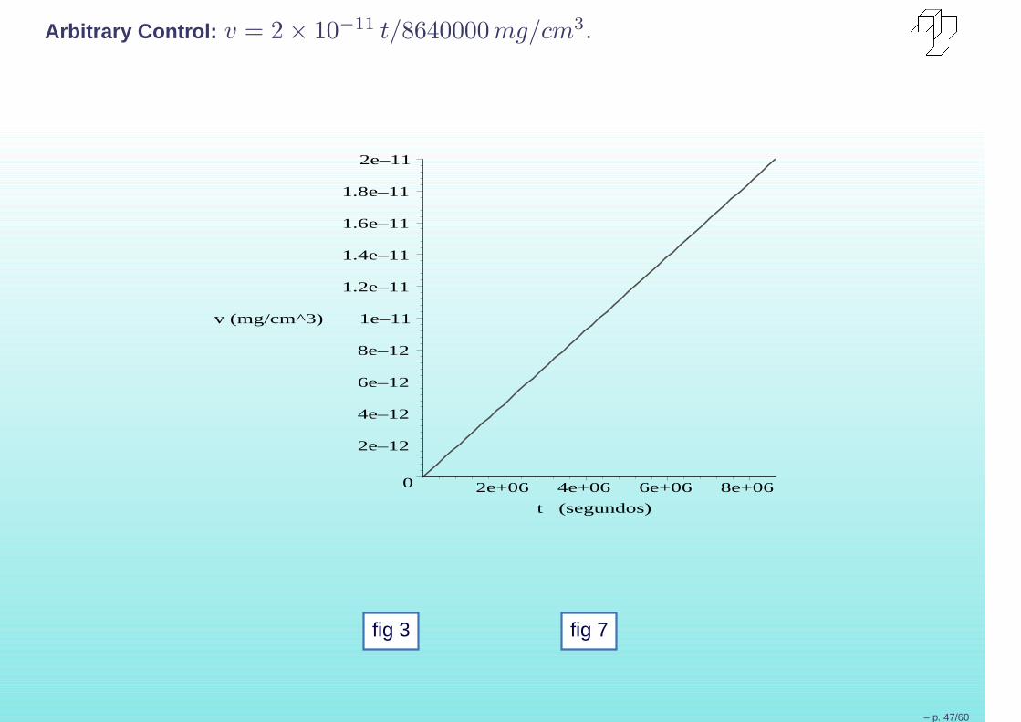
Arbitrary Control: v = 2 × 10⁻¹¹ t/8640000 mg/cm3.
0
2e–12
4e–12
6e–12
8e–12
1e–11
1.2e–11
1.4e–11
1.6e–11
1.8e–11
2e–11
v (mg/cm^3)
2e+06 4e+06 6e+06 8e+06
t (segundos)
fig 3 fig 7
– p. 47/60
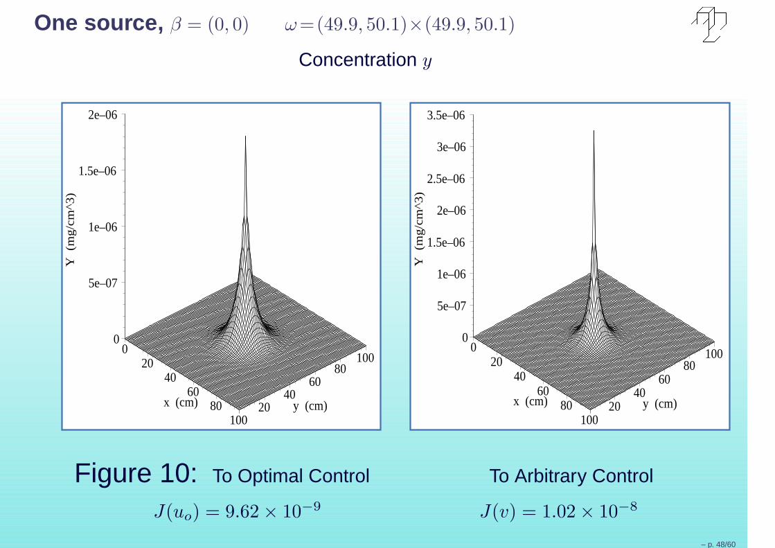
One source, β = (0, 0) ω=(49.9, 50.1)×(49.9, 50.1)
Concentration y
020
4060
80100
x (cm) 2040
6080
100
y (cm)
0
5e–07
1e–06
1.5e–06
2e–06
Y
(mg
/cm
^3)
020
4060
80100
x (cm) 2040
6080
100
y (cm)
0
5e–07
1e–06
1.5e–06
2e–06
2.5e–06
3e–06
3.5e–06
Y
(mg
/cm
^3)
Figure 10: To Optimal Control To Arbitrary Control
J(uo) = 9.62 × 10⁻⁹ J(v) = 1.02 × 10⁻⁸
– p. 48/60
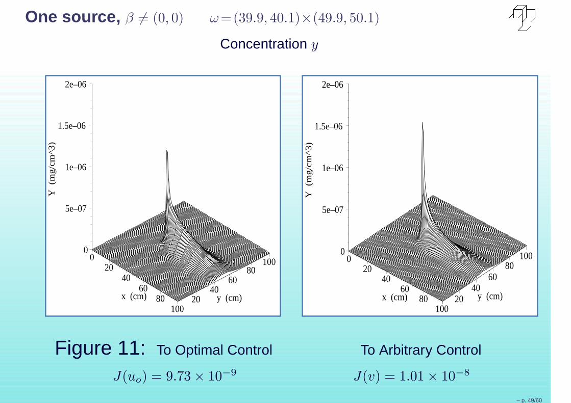
One source, β 6= (0, 0) ω=(39.9, 40.1)×(49.9, 50.1)
Concentration y
020
4060
80100
x (cm) 2040
6080
100
y (cm)
0
5e–07
1e–06
1.5e–06
2e–06
Y (m
g/c
m^3
)
020
4060
80100
x (cm) 2040
6080
100
y (cm)
0
5e–07
1e–06
1.5e–06
2e–06
Y (m
g/c
m^3
)
Figure 11: To Optimal Control To Arbitrary Control
J(uo) = 9.73 × 10⁻⁹ J(v) = 1.01 × 10⁻⁸
– p. 49/60
Comments:
Note that in both graphics, we choose the same places of pollutionentrance.
We observe that the value of J is lesser when the control is optimal,what in fact it would have to occur.
Comparing these graphics of the pollution concentration, we observethat the concentration reaches higher indexes, when we use anarbitrary control. What, also, it is in accordance with our theory.
We made repeated simulations varying the parameters of the model,and in all the cases we evidence the convergence of the method.
– p. 50/60
References RR
1 Lions, J. L., Function Spaces and Optimal Control ofDistributed Systems. Rio de Janeiro, 1980. L.20
2 Lions, J. L., Optimal Control of Systems Gouverned by PartialDifferential Equations, Springer-Verlag, New York, 1971. L.21
3 Lions, J. L., Some Methode in the Mathematical Analysis ofSystems and their Control, Science Press, Beijing, 1981. L.22
4 Lions, J. L., Some Aspects of the Optimal Control of DistributedParameter Systems. Université de Paris and I.R.I.A., RegionalConference Series in Applied Mathematics, 1972, pp. 92. L.23
5 T. J. R. Hughes, The finite Element Method: Linear Static andDynamic Finite Element Analysis, Dover Publications, INC.Mineola, New York, 2000. H.24
– p. 51/60
References
6 CONAMA, Conselho Nacional do Meio Ambiente, D. O. daUnião-30/07/1986, Res. N. 20 de 18 de junho, 1-20, 1986. C.25
7 Pichard, A., Mercury and its Derivatives, Institut National deL’Environnement Industriel et des Risques - INERIS, Version No.1, 2000, 1-45. P.26
8 Banks. H. Thomas, Control and estimation in DistributedParameter System. Masson, Paris, 1992.
9 K. W. Morton, Numerical Solution of Convection - DiffusionProblems. Oxford, UK, 1996.
10 P. Neittaanmaki, D. Tiba, Optimal Control of NonlinearParabolic Systems. Theory, Algorithms and Applications. 1994.
– p. 52/60

THANK YOU
– p. 53/60
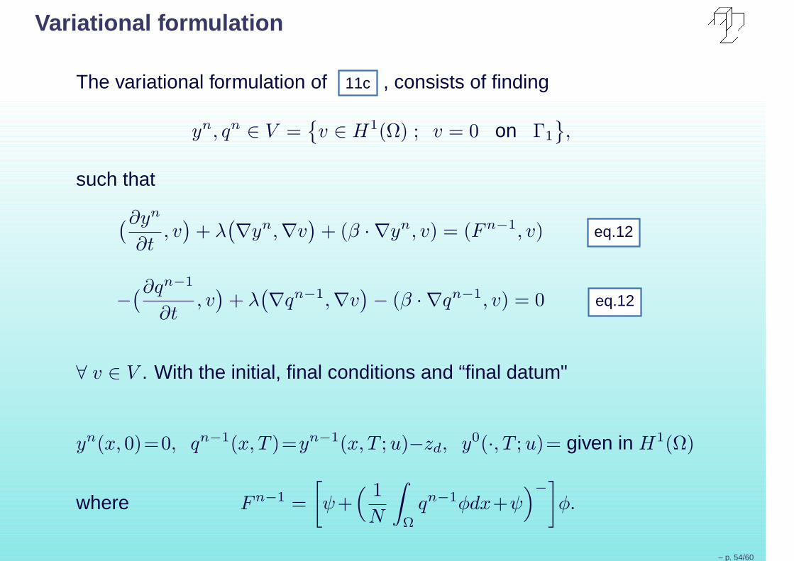
Variational formulation
The variational formulation of 11c , consists of finding
yn, qn ∈ V =
v ∈ H1(Ω) ; v = 0 on Γ1
,
such that
(∂yn
∂t, v
)
+ λ(
∇yn,∇v)
+ (β · ∇yn, v) = (Fn−1, v) eq.12
−(∂qn−1
∂t, v
)
+ λ(
∇qn−1,∇v)
− (β · ∇qn−1, v) = 0 eq.12
∀ v ∈ V . With the initial, final conditions and “final datum"
yn(x, 0)=0, qn−1(x, T )=yn−1(x, T ; u)−zd, y0(·, T ; u)= given in H1(Ω)
where Fn−1 =
[
ψ+( 1
N
∫
Ω
qn−1φdx+ψ)−
]
φ.
– p. 54/60
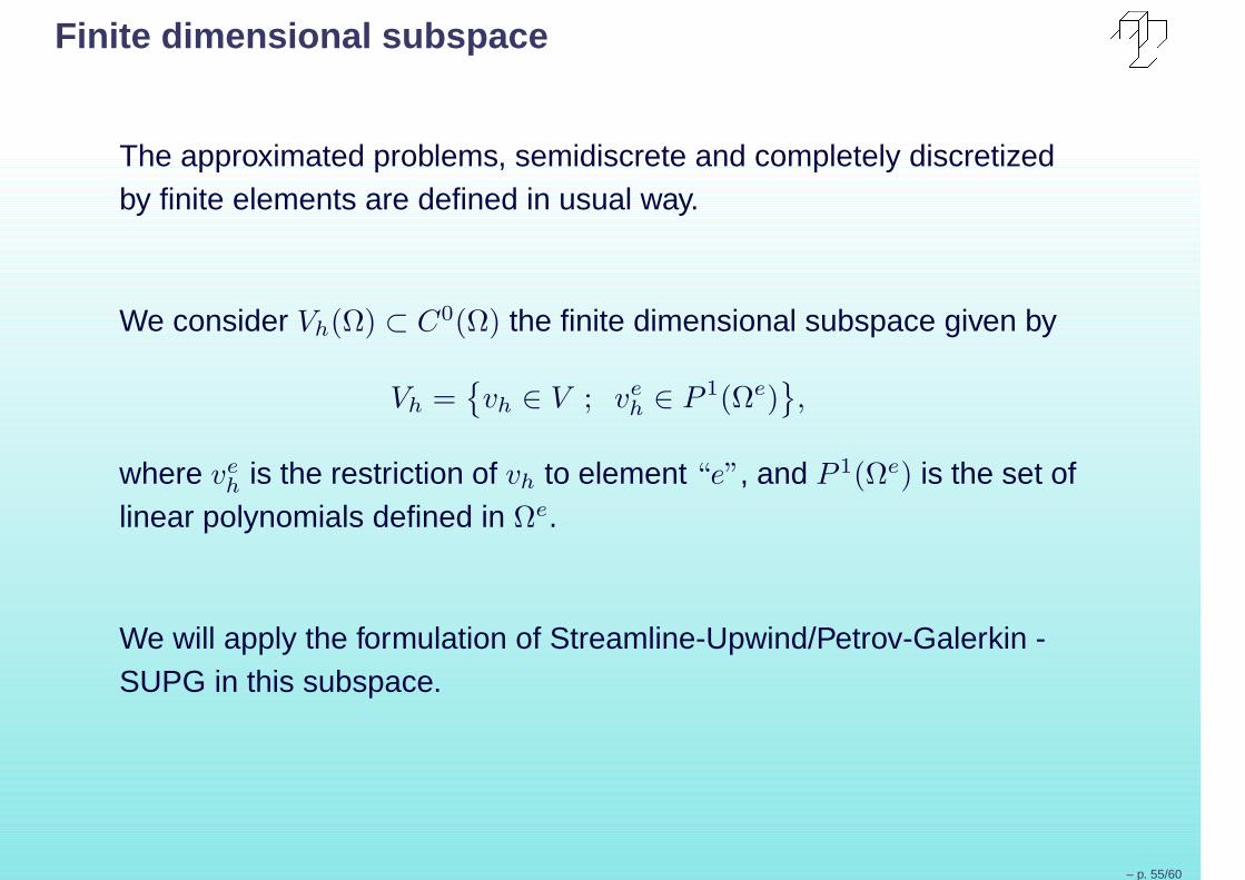
Finite dimensional subspace
The approximated problems, semidiscrete and completely discretizedby finite elements are defined in usual way.
We consider Vh(Ω) ⊂ C0(Ω) the finite dimensional subspace given by
Vh =
vh ∈ V ; veh ∈ P 1(Ωe)
,
where veh is the restriction of vh to element “e”, and P 1(Ωe) is the set of
linear polynomials defined in Ωe.
We will apply the formulation of Streamline-Upwind/Petrov-Galerkin -SUPG in this subspace.
– p. 55/60
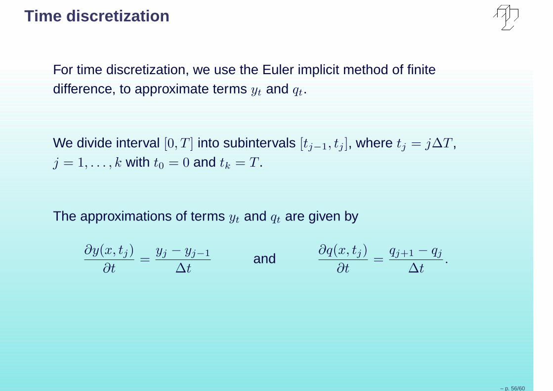
Time discretization
For time discretization, we use the Euler implicit method of finitedifference, to approximate terms yt and qt.
We divide interval [0, T ] into subintervals [tj−1, tj ], where tj = j∆T ,j = 1, . . . , k with t0 = 0 and tk = T .
The approximations of terms yt and qt are given by
∂y(x, tj)
∂t=
yj − yj−1
∆tand
∂q(x, tj)
∂t=
qj+1 − qj
∆t.
– p. 56/60
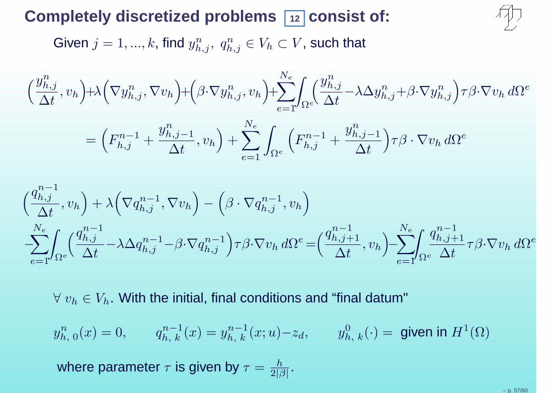
Completely discretized problems 12 consist of:
Given j = 1, ..., k, find ynh,j , qn
h,j ∈ Vh ⊂ V , such that
(ynh,j
∆t, vh
)
+λ(
∇ynh,j ,∇vh
)
+(
β·∇ynh,j , vh
)
+
Ne∑
e=1
∫
Ωe
(ynh,j
∆t−λ∆yn
h,j+β·∇ynh,j
)
τβ·∇vh dΩe
=(
Fn−1h,j +
ynh,j−1
∆t, vh
)
+
Ne∑
e=1
∫
Ωe
(
Fn−1h,j +
ynh,j−1
∆t
)
τβ · ∇vh dΩe
(qn−1h,j
∆t, vh
)
+ λ(
∇qn−1h,j ,∇vh
)
−(
β · ∇qn−1h,j , vh
)
−
Ne∑
e=1
∫
Ωe
(qn−1h,j
∆t−λ∆qn−1
h,j −β·∇qn−1h,j
)
τβ·∇vh dΩe =(qn−1
h,j+1
∆t, vh
)
−
Ne∑
e=1
∫
Ωe
qn−1h,j+1
∆tτβ·∇vh dΩe
∀ vh ∈ Vh. With the initial, final conditions and “final datum"
ynh, 0(x) = 0, qn−1
h, k (x) = yn−1h, k (x; u)−zd, y0
h, k(·) = given in H1(Ω)
where parameter τ is given by τ = h2|β| .
– p. 57/60
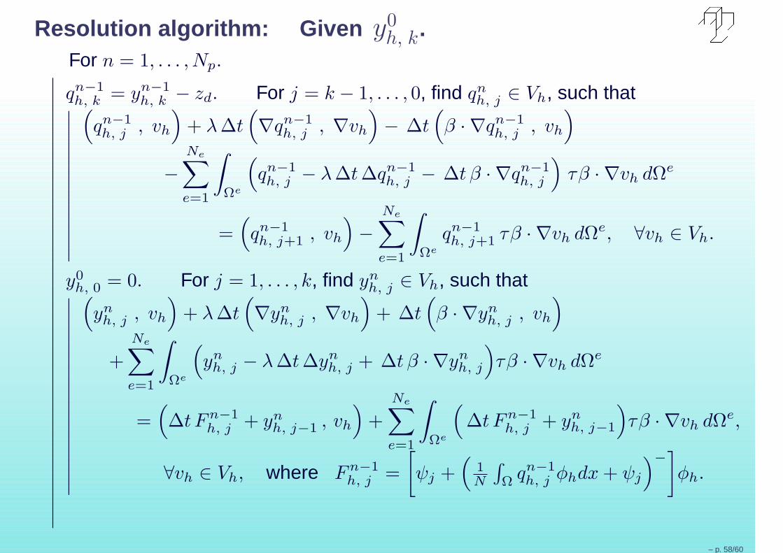
Resolution algorithm: Given y0h, k.
∣
∣
∣
∣
∣
∣
∣
∣
∣
∣
∣
∣
∣
∣
∣
∣
∣
∣
∣
∣
∣
∣
∣
∣
∣
∣
∣
∣
∣
∣
∣
∣
∣
∣
∣
∣
∣
∣
∣
∣
∣
∣
For n = 1, . . . , Np.∣
∣
∣
∣
∣
∣
∣
∣
∣
∣
∣
∣
∣
∣
∣
∣
∣
∣
∣
∣
∣
∣
∣
∣
∣
∣
∣
∣
∣
∣
∣
∣
∣
∣
∣
∣
∣
∣
∣
qn−1h, k = yn−1
h, k − zd. For j = k − 1, . . . , 0, find qnh, j ∈ Vh, such that
∣
∣
∣
∣
∣
∣
∣
∣
∣
∣
∣
∣
∣
(
qn−1h, j , vh
)
+ λ ∆t(
∇qn−1h, j , ∇vh
)
− ∆t(
β · ∇qn−1h, j , vh
)
−
Ne∑
e=1
∫
Ωe
(
qn−1h, j − λ ∆t ∆qn−1
h, j − ∆t β · ∇qn−1h, j
)
τβ · ∇vh dΩe
=(
qn−1h, j+1 , vh
)
−
Ne∑
e=1
∫
Ωe
qn−1h, j+1 τβ · ∇vh dΩe, ∀vh ∈ Vh.
y0h, 0 = 0. For j = 1, . . . , k, find yn
h, j ∈ Vh, such that∣
∣
∣
∣
∣
∣
∣
∣
∣
∣
∣
∣
∣
∣
∣
∣
∣
(
ynh, j , vh
)
+ λ ∆t(
∇ynh, j , ∇vh
)
+ ∆t(
β · ∇ynh, j , vh
)
+
Ne∑
e=1
∫
Ωe
(
ynh, j − λ ∆t ∆yn
h, j + ∆t β · ∇ynh, j
)
τβ · ∇vh dΩe
=(
∆t Fn−1h, j + yn
h, j−1 , vh
)
+
Ne∑
e=1
∫
Ωe
(
∆t Fn−1h, j + yn
h, j−1
)
τβ · ∇vh dΩe,
∀vh ∈ Vh, where Fn−1h, j =
[
ψj +(
1N
∫
Ωqn−1h, j φhdx + ψj
)−]
φh.
– p. 58/60
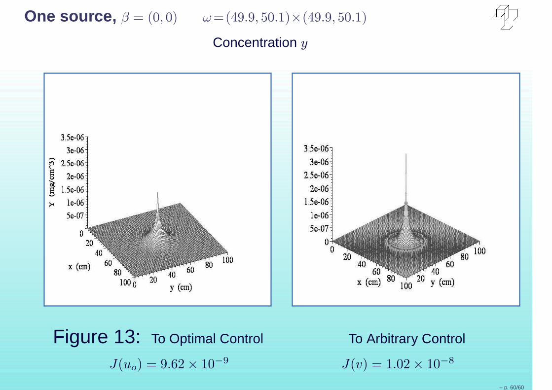
One source, β = (0, 0) ω=(49.9, 50.1)×(49.9, 50.1)
Concentration y
Figure 13: To Optimal Control To Arbitrary Control
J(uo) = 9.62 × 10⁻⁹ J(v) = 1.02 × 10⁻⁸
– p. 60/60