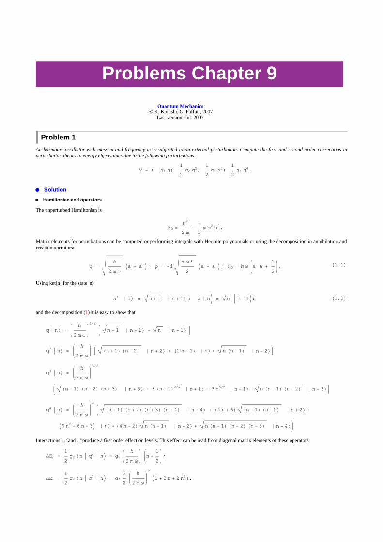
Problems Chapter 9

Quantum Mechanics © K. Konishi, G. Paffuti, 2007

Last version: Jul. 2007

Problem 1

An harmonic oscillator with mass m and frequency Ω is subjected to an external perturbation. Compute the first and second order corrections inperturbation theory to energy eigenvalues due to the following perturbations:

V = : g1 q;1

2 g2 q2;

1

2 g3 q3;

1

2 g4 q4.

æ Solution

à Hamiltonian and operators

The unperturbed Hamiltonian is

H0 =p2

2 m+

1

2 m Ω

2 q2.

Matrix elements for perturbations can be computed or performing integrals with Hermite polynomials or using the decomposition in annihilation andcreation operators:

(1.1)q =Ñ

2 m Ω Ia + aÖM; p = -ä

m Ω Ñ

2 Ia - aÖM; H0 = Ñ Ω aÖ

a +1

2.

Using ket[n] for the state |n\(1.2)aÖ È n\ = n + 1 È n + 1\ ; a È n_ = n Ë n - 1_;

and the decomposition (1) it is easy to show that

q È n\ =Ñ

2 m Ω

12 n + 1 È n + 1\ + n È n - 1\

q2 É n] =Ñ

2 m Ω Hn + 1L Hn + 2L È n + 2\ + H2 n + 1L È n\ + n Hn - 1L È n - 2\

q3 É n] =Ñ

2 m Ω

32

Hn + 1L Hn + 2L Hn + 3L È n + 3\ + 3 Hn + 1L32 È n + 1\ + 3 n32

È n - 1\ + n Hn - 1L Hn - 2L È n - 3\

q4 É n] =Ñ

2 m Ω

2

Hn + 1L Hn + 2L Hn + 3L Hn + 4L È n + 4\ + H4 n + 6L Hn + 1L Hn + 2L È n + 2\ +

I6 n2 + 6 n + 3M È n\ + H4 n - 2L n Hn - 1L È n - 2\ + n Hn - 1L Hn - 2L Hn - 3L È n - 4\Interactions q2and q4produce a first order effect on levels. This effect can be read from diagonal matrix elements of these operators

DEn =1

2 g2 Yn É q2 É n] = g2

Ñ

2 m Ω n +

1

2;

DEn =1

2 g4 Yn É q4 É n] = g4

3

2

Ñ

2 m Ω

2

I1 + 2 n + 2 n2M.Operators q and q3produce a shift at second order. The first order contribution is zero by parity conservation and this is confirmed from absence of

diagonal elements intheir matrix elements. At second order the shift in energy levels is

Operators q and q3produce a shift at second order. The first order contribution is zero by parity conservation and this is confirmed from absence of

diagonal elements intheir matrix elements. At second order the shift in energy levels is

DEH2L= â

s

' XΨ0 È V È s\ 1

E0 - Es Xs È V È Ψ0\.

Only a finite number of intermidiate states contribute to the sum.

ã Operator q

DEnH2L

= g12

È Xn È q È n - 1\ È2En - En-1

+È Xn È q È n + 1\ È2

En - En+1

= -1

2 g12

m Ω2.

This result is obvious, a linear term in q canbe reabsorbed by a translation of the quadratic potential:

1

2 m Ω

2 q2 + g1 q =

1

2 m Ω

2 q +

g1

m Ω2-

1

2 g12

m Ω2.

ã Operator q3

The only contributions different from zero are

DEnH2L

=1

4 g32

É Yn É q3 É n - 1] È2En - En-1

+

É Yn É q3 É n + 1] È2En - En+1

+

É Yn É q3 É n - 3] È2En - En-3

+

É Yn É q3 É n + 3] È2En - En+3

=

-

g32

4 Ñ Ω

Ñ

2 m Ω

3

I30 n2 + 30 n + 11M.ã Operator q4

The only contributions different from zero come from transitions to intermidiate states n, n±2, n±4. A computation similar to the one above gives, forsecond order contribution:

DEnH2L

= -g42

4 Ñ Ω

Ñ

2 m Ω

4

I68 n3 + 102 n2 + 118 n + 42M.

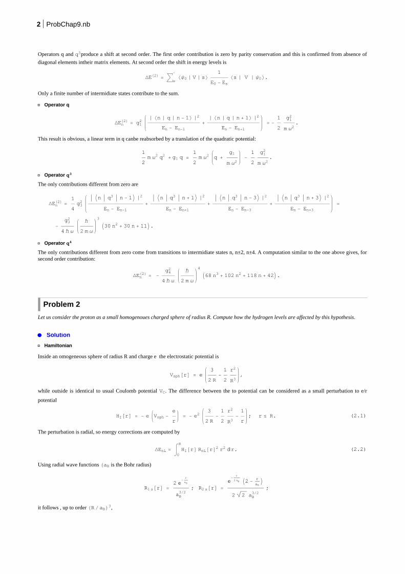
Problem 2

Let us consider the proton as a small homogenoues charged sphere of radius R. Compute how the hydrogen levels are affected by this hypothesis.

æ Solution

ã Hamiltonian

Inside an omogeneous sphere of radius R and charge e the electrostatic potential is

Vsph@rD = e3

2 R-1

2 r2

R3,

while outside is identical to usual Coulomb potential VC. The difference between the to potential can be considered as a small perturbation to e/r

potential

(2.1)HI@rD = - e Vsph -e

r= - e2

3

2 R-1

2 r2

R3-1

r; r £ R.

The perturbation is radial, so energy corrections are computed by

(2.2)DEnL = à0

R

HI@rD RnL@rD2 r2 âr.

Using radial wave functions HaB is the Bohr radius)

R1 s@rD =2 ã

-r

aB

aB32 ; R2 s@rD =

ã-

r

2 aB I2 -r

aBM

2 2 aB32 ;

it follows , up to order HRaBL3,

2 ProbChap9.nb

DE1 s =2

5

R

aB

2 e2

aBº

2

5

R

aB

2

a.u.; DE2 s =1

20

R

aB

2 e2

aBº

1

20

R

aB

2

a.u. .

Energy shift for states with higher L are depressed, since radial wave functions decrease as rL. For p states we expect DE ~ HRaBL4 a.u., as is

easily confirmed for example computing the correction to 2p state:

R2 p@rD =ã

-r

2 aB r

2 6 aB52 ; DE2 p =

e2 R4

1120 aB5

+ O@RD5 >1

1120

R

aB

4

a.u.

ã A different approach

Let us call e Ρ the charge density of the nucleus, or in general Z e Ρ for a nucleus with Z protons. If V is the electrostatic potential we can write thegeneric energy shift as

(2.3)DE = - e à d3 r Ψ@rD¤2 V -

Ze

r> - e Ψ@0D¤2 à d

3 r V -

Ze

r.

Last approximate equality take care of the fact that V differ from Z/r only at very small distances, and clarify that in practice only s-states are affectedby the perturbation. Using the identity

1 =1

6 D r2,

and integrating by parts eq (3) can be rewritten as

DE =

- e Ψ@0D¤2 à d3 r

1

6 r2 D V -

Ze

r= - e Ψ@0D¤2

1

6 à d

3 r r2 I4 Π e Ρ - Z e 4 Π ∆

3@rDM =2

3 Π Z e¤2 Ψ@0D¤2 Yr2].

The measure of DE would be a direct measure of mean square radius of the (charge of the) nucleus.

Problem 3

Let us suppose that Coulomb potential has a behaviour 1r1+¶, with ¶ ` 1. Compute the effect on hydrogen levels and derive a bound on ¶

comparing the 2p-2s induced energy gap with the observed Lamb shift correction. The theory agree with experiment at leat up to ∆E/h = 104 kHz.

æ Solution

ã Hamiltonian and perturbation

In this problem we will use atomic units |e|= Ñ=m = 1. We can consider the difference between the supposed Coulomb law and usual -1/r law as aperturbation

HI = -1

r1+¶

-1

r.

Energy corrections are given by the mean value of HIon eigenfunctions of hydrogen atom. Radial wave functions for 1s, 2s, 2p states are, in atomic

units:

R1 s@rD = 2 ã-r ; R2 s@rD =

ã-r2 H2 - rL2 2

; R2 p@rD =ã-r2 r2 6

.

A simple integration gives (energies in atomic units)

DE1 s = 2¶GH2 - ¶L - 1 ; DE2 s =

1

8II¶

2- ¶ + 2M GH2 - ¶L - 2M; DE2 p =

1

24HGH4 - ¶L - 6L.

G is the Euler Gamma function. For small ¶ a Taylor expansion gives

DE2 s - DE2 p >¶

12 a.u. =

¶

6 Ry.

The agreement between theory and experiment for the computed Lamb shift between 2 s12 and 2 p12 levels imply the bound

É ¶ É < 6×104 kHz h Ry > 1.8×10

-11.

It can be useful to note the following conversion factors (h is Planck constant, i.e. 2 Π Ñ)

ProbChap9.nb 3

(3.1)Ry

h= 3289841.9680 GHz;

Ry

h c>1.09737´10

7

Meter=

1.09737´105

cm.

Problem 4

Compute the effect of an electric field on the levels of a charged harmonic oscillator. Compute induced electric dipole and verify Feynman-Hellmanntheorem.

æ Solution

ã Hamiltonian and perturbation

This is the simplest model for studying the effect of an electric field on a quantum system. Let us denote by E the external electric field and by e thecharge of the oscillator. The Hamiltonian is

(4.1)H =p2

2 m+

1

2 m Ω

2 q2 - e E q =

p2

2 m+

1

2 m Ω

2 q -

e E

m Ω2

2

-1

2 e2 E2

m Ω2

The change of variable

P = p ; Q = q -e E

m Ω2

is a unitary (and classically canonical) transformation, then the physics do not change and we can consider as Hamiltonian

(4.2)H =P2

2 m+

1

2 m Ω

2 Q2 -

1

2 e2 E2

m Ω2;

which differ from unperturbed hamiltonian only by an additive constant. All levels are shifted by the same E dipendent constant

(4.3)DE = -1

2 e2 E2

m Ω2.

The reader can check the result in perturbation theory as an exercise (see also prob.[1]). Let us make some comments on this seemingly trivialexercise.

The unperturbed system is invariant under parity, q ® - q and the system, as must be well known by the reader, has no dipole moment in stationarystates.

The perturbed system is not parity invariant and the system has a dipole in stationary states (classically an induced dipole). The Hamiltonian (2) is

invariant under the transformation Q ® - Q, which is not the parity of the system. By this symmetry the mean value of Q on stationary states of (2)

is zero. On exact stationary states, i.e. eigenstates of (2), we have the induced dipole (use the definition of Q):

XΨ È d È Ψ\ º e XΨ È q È Ψ\ = e XΨ È Q È Ψ\ + e [Ψe E

m Ω2Ψ_ =

e2 E

m Ω2.

The coefficient of propotionality between induced dipole and external field has dimension of a volume and is called polarizability of the system.In our case

d = Α E; Α =e2

m Ω2.

Interaction lower energy of the system, see (3), and is written in the same form as classical dipole induced interaction:

DE = -1

2 e2 E2

m Ω2= -

1

2 Α E2

We can verify in this simple system Feynman - Hellmann theorem, which reads in this case

(4.4)¶DE

¶E= [Ψ

¶H

¶EΨ_.

The l.h.s. of (4) is -Α E. The r.h.s. is:

[Ψ¶H

¶EΨ_ = - e XΨ È q È Ψ\ = -

e2 E

m Ω2= - Α E,

verifying the theorem.

Problem 5

4 ProbChap9.nb

Problem 5

Solve the two level system

H = E0 +-E1 -∆

-∆* E1º E0 - Σ ×B

and compare with perturbation theory results as B® 0 . Discuss how the phases of eigenstates depend on B.

æ Solution

à Exact solution

Our problem has only two states, conventionaly denoted by È +\ and È -\ . The constant E0 given in the text of the exercise is just an additive constant to

the energy and will be disregarded from now on. The Hamiltonian can be considered in a form

(5.1)H = H0 + V; H0 =-E1 0

0 E1; V =

0 -∆

-∆* 0;

and studied exactly or with perturbation theory. The eigenvalues are trivially found solving the quadratic equation det(Λ - H) = 0, but as an exercisewe want to follow another more instructive path. System (1) can be considered as the Hamiltonian of a spin 1/2 interacting with a magnetic field.Magnetic interaction for spin 1/2 is described by -Μ Σ·B where Μ is the magnetic moment, B the magnetic field and Σ the Pauli matrices. With thesubstitution B ® Μ B our system is indeed a magnetic Hamiltonian. If we write

(5.2)∆ = D ã-ä j; H = -Σ ×B; Σx =

0 1

1 0; Σy =

0 -ä

ä 0; Σz =

1 0

0 -1.

we have

H = -E1 HD Cos@jD - ä D Sin@jDL

HD Cos@jD + ä D Sin@jDL -E1,

and we can identify the components of our magnetic field with

(5.3)Bx = D Cos@jD; By = D Sin@jD; Bz = E1; B = È B È = D2

+ E12 .

In our magnetic analogy the perturbation treatment would consist in adding a transverse magnetic field of strength D to a magnetic field E1along z

(the direction of the magnetic field is what identify z direction). In this language it is clear that we can choose the x direction along the transverse fieldand put j = 0, i.e. kill y-component of B field. From now on we adopt this convention and write DÎ R instead of ∆. Let us note that we can alsochoose j = Π, than have in effect both positive and negatives vaules for D. A priori the two choices are distinct and this will have some consequencebelow.

The reader now has 3 choices, he can forget this discussion and assume from the beginning a real Hamiltonian, or he can read the note at the end ofthis subsection to understand for a generic system (without a real magnetic field) what it means the choice ∆ real. The third (better) choice is to try tounderstand by himself the question.

In the real form H is given by

H = - K E1 D

D -E1O = - Σx Bx - Σz Bz = - B

Cos@ΘD Sin@ΘDSin@ΘD -Cos@ΘD .

(5.4)

x

z

BΘ

Bx = BSin@ΘD; Bz = B Cos@ΘD; Sin@ΘD =D

B; B = E1

2+ D

2

and it is apparent that we can diagonalize the Hamiltonian by bringing z axis along B. The rotation of reference frame is an anticlockwise rotationaround y axis, i.e.

(5.5)R = ExpBäΘ

2 ΣyF = CosB Θ

2F + ä Σy SinB Θ

2F =

CosA Θ

2E +SinA Θ

2E

-SinA Θ

2E CosA Θ

2E

In the rotated basis the Hamiltonian will be diagonal, and in effect the reader can check that

(5.6)R H RÖ= - B Σz.

The new basis vectors will be

ProbChap9.nb 5

(5.7)È g\ = RÖ È +\ =CosA Θ

2E -SinA Θ

2E

+SinA Θ

2E CosA Θ

2E

1

0=

CosA Θ

2E

SinA Θ

2E ; È e\ = RÖ È -\ =

-SinA Θ

2E

CosA Θ

2E .

N.B. We remember that basis vectors transform as the inverse rotation, see notebook [**] for more details.

The reader can verify directly that

(5.8)H È g\ = - B È g\; H È e\ = B È e\;| g\ and È e\ are respectively the ground state and the excited state of the system with energy eigenvalues ¡ B = ¡ E1

2 + D2

ã The choice of initial phases

The reader can skip this subsection in a first reading.

The thesis is that we can always choose the phases of our states in such a way that ∆ is real. This is trivially true in the sense that if we choose as basisvectors

(5.9)È a\ = ã-ä j2

È +\; É b] = ã+ä j2

È -\;the Hamiltonian haa the same diagonal matrix elements

Xa È H È a\ = X+ È H È +\ = - E1; Xb È H È b\ = X- È H È -\ = E1;

and real off diagonal elements

Xa È H È b\ = ãä j X+ È H È -\ = - D; Xb È H È a\ = ã

-ä j X- È H È +\ = - D.

The choice of the phase of basis functions can always been made by a unitary transformation so the physics is not changed. Let us note that È a\ and Èb\ are obtained from È +\ and È -\ states by the unitary transformation Exp[-ä j/2 Σz]:

È a\ = Exp@-ä j Σz 2D È +\; È b\ = Exp@-ä j Σz 2D È -\;and this is exactly how a rotation of an angle j acts on spinors in the magnetic analogy.

From a physical point of view we can state the same conclusions with a different perspective. In two dimensions we have only 4 independenthermitian matrices, the identity and the four Pauli matrices, each matrix canbe written as a linear superposition of these matrices. The "maximalabelian set" of observables, neglecting identity, is formed by only one element, one of the Pauli matrices, by convention let us choose Σz. Our states

are labeled by eigenvalues of this observable, nothing else, and in effect the two states È a\ and È +\ for example belong to the same eigenvalue of Σz.

To pass from rays to vectors in Hilbert space we have to make a choice for phases, and this means to choice È a\ or È +\ . To avoid misunderstandingsthis does not means that we can change the phases in such a way that every linear combination È Ψ> = c1È +\ + c2È -\ has real coefficients: once we

have choosen a phase for basis vectors this choice is valid for every linear combination.

There is one more subtle point. When we write Σ matrices in the usual form we have in effect done a choice of phases, for example Σy has purely

imaginary elements, how this combine with the above freedom in phases? In effect when we have stated in the main text that the usual representationof spin 1/2 is The representation of SU(2) of dimension 2 it was understood up to unitary tansformations. Which means again that we can alwayschoose the phases in such a way the Σ matrices have the usual form. Now if we do a unitary transformation on a basis which satisfy usual conventionon the phases we obtain again a representation with the correct phases. In effect the only point is the state È -\ which is defined, without additionalphases, as HΣx- äΣy)/2 È +\ . If we perform a unitary transformation both matrices and states change. Under the transformation R = Exp[-ä j Σz 2Dfor

example:

Σi ® Si = R Σi RÖ

and under a unitary transformation all linear relation, and commutation relations, remain invariant, in particular the new È -\ state, which is È b\ , isobtained by applying the new sigma matrices, S, to È a\ and everything works in exactly the same way.

In effect after the transformation we had to write S instead of Σ for matrices and spin operators, but as these operators on the new basis have thesame matrix elements as old operators inthe old basis we use the same symbols, as is always more or less implicitily done.

à Non degenerate perturbation theory

Simple perturbation theory on non degenerate levels can be applied for D ` E1. In absence of perturbation -B Sin[Θ] Σx ground and excited state are È+\ and È -\ . As X+ È Σx È +\ = 0 = X- È Σx È -\ corrections to eigenvalues start from second order and we have

DEg = - E1 + D2 X+ È Σx È -\

1

-2 E1 X- È Σx È +\ = - E1 1 +

1

2 D2

E12

;

DEe = E1 + D2 X+ È Σx È -\

1

2 E1 X- È Σx È +\ = E1 1 +

1

2 D2

E12

.

These results are in agreement with Taylor expansion of exact results (8), as for small D

6 ProbChap9.nb

B = E12

+ D2

> E1 1 +1

2 D2

E12

.

The eigenstates have a first order correction. Using the general formula

∆ È n\ = âs

' 1

En - Es È s\ Xs È V È n\,

we have for first order eigenstates with V = - D Σx:

È g\ > È +\ +D

2 E1È -\ > È +\ +

Θ

2 È -\ ; e = È -\ -

D

2 E1È +\ > È -\ -

Θ

2È +\;

which are first order expansion of (7).

à Degenerate perturbation theory

As E1 ® 0 , and in general for |E1 È ` D previous formulae do not apply and in this regime we have to switch to degenerate perturbation theory. To

see exactly wy perturbation theory on degenerate levels is different let us consider the exact solution (7). As Tan[Θ] = D E1we see that the vaule of Θ

in the degeneration limit E1 ® 0depends on the sign of D

limE1®0

Θ =Π 2; if D E1 > 0

-Π 2; if D E1 < 0

Accordingly for ground state, as an example

limE1®0+

È g\ =

H È +\ + È -\L 2 º Ë S^ ; if D > 0

H È +\ - È -\L 2 º Ë A^ ; if D < 0

i.e. when we switch off the perturbation D we do not know in advance which state of the two dimensional space spanned by È +\ and È -\ correspondto ground and excited state.

States È S\ ans È A\ diagonalize the degenerate hamiltonian but we see that È g\ is not analytic in D, precisely is discontinuous for D = 0. A similar thinghappens for eigenvalues. In the degenerate limit eigenvalue are ± |D| which are continuous but not derivable in D = 0.

This picture has some relevant consequences. If we imagine to vary smoothly the external field, the eigenvectors follow the variation except if wepass through the singular point E1 = 0, D = 0, where there is an abrupt change. This is wy adiabatic theorem does not work if in the evolution the

system goes through a degeneracy point.

This breaking of adiabatic theorem is even more clear if we switch on the y component of the magnetic field. In the general case

Bx = B Sin@ΘD Cos@jD; By = B Sin@ΘD Sin@jD; Bz = B Cos@ΘD; B = E12

+ D2 ;

As already noted the y component can be reabsorbed by an anticlockwise rotation of j around z axis of the reference frame. After rotation the newunperturbed eigenstates will be

(5.10)È +\' = RzÖ@jD È +\ = ExpB-ä

j

2 ΣzF È +\ = ExpB-ä

j

2F È +\ ; È -\' = Exp@+ä j 2 D È -\ .

For these states everything works as before the only difference being that now D, the modulus of transverse field, is necessarly positive. In thedegerate limit

È g\ =1

2

H È +\' + È -\' L =1

2

ExpA-ä

j

2E

ExpA+äj

2E .

The ground state has now a continuous range of variation, not only a double determination as before. Which of the infinite set corrspond to the trueground state depends on the actual value of j.

The general solution, see (7), is

(5.11)È g\ = CosB Θ

2F È +\' + SinB Θ

2F È -\' =

CosA Θ

2E ExpA-ä

j

2E

SinA Θ

2E ExpA+ä

j

2E .

We note that È g\ change its sign as j varies from 0 to 2Π, like spinor (we remember that in principle our system has nothing to do with a real spinor).This effect is a particularly simple form of Berry phase.

Consider a system in which we vary adiabatically the transverse field around a circle, i.e. j varies from 0 to 2Π. In principle we can locally adjust thephase of our eigenstates in such a way that the ground state follows the variation of the field, why we obtain an additive minus sign after a cicle? Letus consider the infinitesimal variation of the state under a change of a set of parameters Λi

ProbChap9.nb 7

(5.12)Xg È ¶

¶Λi

È g\if we can reset to zero expression (12) with a change of phase, then we can choose our phases in such a way that they follow variations of external

field. In the present case our parameters are Θ and j and we have from (11)

Xg È ¶

¶Θ È g\ = 0; Xg È

¶

¶j È g\ = -

ä

2 Cos@ΘD.

Consider now a totation of the transverse field at fixed Θ. To reabsorb the phase variation we would need a change of phase

È g\ ® Exp@ä ΑD È g\; Α@jD =1

2 Cos@ΘD j,

but the function Α is not monodrome in j, i.e. is not a function, so it is not allowed, and we cannot reabsorb the phase variation in a closed loop by aglobal defined Α. The amount of phase change under a cyclic variation of external condition is substantially the Berry phase of the system.

Problem 6

A two level system as that of problem [5] can be considere as a simplified model of an ammonia molecule, NH3. Nitrogen's position with respect to

the plane of 3 hydrogen atoms select, classically, two equivalent configuration. Define a parity operator for this model and discuss its property. Studythe effect of an electric field on the system.

æ Solution

à Description of the model

An ammonia molecule can be described by three coplanar hydrogen atoms, (x,y) plane, and a nitrogen outside the plane. The system admits aspecular configuration obtained by a reflection across (x,y) plane, i.e. z®-z, then a second position for nitrogen atom, classically equivalent to thefirst one, exists. Classically the two position are separated by a potential barrier, and are local minima of the potential energy. Tunnel effect allow amixing between these two configurations. The situation is described pictorially inthe folowing figure:

8 ProbChap9.nb

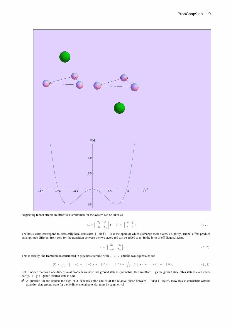
-1.5 -1.0 -0.5 0.5 1.0 1.5z

-0.5

0.5

1.0

U@zD

Neglecting tunnel effects an effective Hamiltonian for the system can be taken as

(6.1)H0 =E0 0

0 E0; P =

0 1

1 0.

The basis states correspond to classically localized states, È +\ and È -\ . P is the operator which exchange these states, i.e. parity. Tunnel effect producean amplitude different from zero for the transition between the two states and can be added to H0 in the form of off diagonal terms

(6.2)H =E0 -D

-D E0.

This is exactly the Hamiltonian considered in previuos exercize, with E1 = 0,and the two eigenstates are

(6.3)È g\ =1

2 J È +\ + È -\ L º È S\; È e\ =

1

2 H È +\ - È -\ L º È A\;

Let us notice that for a one dimensional problem we now that ground state is symmetric, then in effect È g\ is the ground state. This state is even underparity, PÈ g\ = È g\ while excited state is odd.

A question for the reader: the sign of D depends onthe choice of the relative phase between È +\ and È -\ states. How this is consistent withtheassertion that ground state for a one dimensional potential must be symmetric?

ProbChap9.nb 9

à Electric field

The charge distribution in configurations È +\ and È -\ is asymmetric, due to greater electronegativity of Nitrogen. Classically this that these statespossess an electric dipole. We can describe this effect with

(6.4)d = X+ È e z È +\ ; - d = X- È e z È -\ ; X- È e z È +\ = 0;

We note that the first equality is a definition, while the other two equalities are a consequence of our model.

Let us assume that our states are (relatively ) real, e.g. are approximate real solution of one dimensional Schrödinger equation. The parity operator P

must acts on z as P z P-1º P z P = - z (we used P2= 1), then

X- È z È -\ = X+ È P z P È +\ = - X+ È z È +\ = -d.

For the third equality,using reality of matrix elements:

X- È z È +\ = X+ È P z P È -\ = - X+ È z È -\ = - HX- È z È +\L*= - X- È z È +\ Þ X- È z È +\ = 0.

Let us note that states È +\ and È -\ are not eigenstates of Hamiltonian (2) so the general theorem about absence of electric dipole moment on stationary

states do not apply. If we neglect tuneling the states are eigenstates of (1) but the system is degenerate and again the theorem does not apply.

If we switch on an electric field E, this field will couple with dipole mpoment and the Hamiltonian becomes

(6.5)H = E0 +-d E -D

-D d E.

The Hamiltonian (5) is identical to that of problem [5] and we can write at once anergy levels and eigenstates:

(6.6)E = E0 ¡ D2

+ d2 E2 ; È gE\ =CosA Θ

2E

SinA Θ

2E ; È eE\ =

-SinA Θ

2E

CosA Θ

2E ; Tan@ΘD =

D

d E.

Equation (6) explain in a simple way how in quantum mechanics we can have approximatively a linear Stark effect, which mimics the classicalinteraction - d E. In the limit of large fields with respect the transition matrix element, or energy splitting, dE p D, we have Θ ® 0 and

E = E0 ¡ d E; È g\E >1

0; È e\E =

0

1;

We have classical linear dependency on electric field wich mimics a permanent dipole of the system. Eigenstates are "frozen" toward classicallocalized states. In these states, see eq.(4)

XgE È e z È gE\ > d ; XeE È e z È eE\ > - d .

In effect permanent static dipole, polarizability etc, are defined in the limit of vanishing extenal field. Let us assume d E ® 0+, then Θ ® Π/2 and we

have

(6.7)E = E0 ¡ D +1

2

d2 E2

D;

È gE\ =1

2

1 +d E

2 D È +\ + 1 -

d E

2 D È -\ ;

È eE\ =1

2

1 -d E

2 D È -\ - 1 +

d E

2 D È +\ ;

From eq.(7) we see that Stark effect is indeed quadratic with polarizations

E - E0 = -1

2 Α E2; Αg =

d2

D; Αe = -

d2

D.

We note that for excited states polarizability has a negative sign, so the atoms behave at the opposite of usual dielectrics (they are repelled in anexternal gradient field).

These result are confirmed by taking the mean value of the dipole operator on exact eigenstates inthe limit of small field:

XgE È e z È gE\ >d2

D E ; XeE È e z È eE\ > -

d2

D E .

Problem 7

Study the effect of an electric field (Lo Surdo-Stark effect) on the n=2 states of the hydrogen atom, neglecting the effects of spin.

æ Solution

10 ProbChap9.nb

æ

Solution

à General properties

In the non relativistic approximation the n=2 level of hydrogen atom has degeneration 4, (we neglect spin degrees of freedom): there is one 2s stateand three 2p states. Let us choose as quantization axis (z axis) the direction of the electric field E. The Hamiltonian is

(7.1)H =p2

2 m-

e2

r- e z E

e is the electron charge. H is invariant for rotations around z axis, then Lz can be diagonalized simultaneously with H. In perturbation theory this is

reflected by the fact that the term e z E has no matrix elements between states with different eigenvalues of Lz.

The Hamiltonian is also invariant under reflection R across a plane containing z axis, ex. y ® - y. Classically the porjections of angular momentumalong z change sign under this operation, the same is true in quantumtheory. In angular coordinates this symmetry is equivalent to j ® - j and withour choice of phase for spherical harmonics

(7.2)YLmHJ, -jL H-1Lm YL-mHJ, jL; Þ R É n, L, m] = H-1Lm É n, L, - m].

As H commutes with R the states with opposite m (eigenvalue of LzLwill remain degenerate even in presence of the perturbation. The same

conclusion can be drawn using time reversal symmetry and the relation

YL-mHJ, jL H-1Lm YL

mHJ, jL­.

à Perturbation theory

Perturbation theory on n = 2 level is a typical example of degenerate perturbation theory and we have to diagonalize matrix elements of the perturba-tion on the subspace spanned by states 2s, 2p. We have seen some selection rules in previous section, to this we add that z is odd with respect parity,so only matrix elements between different parity can be different from zero.

Denoting the states with È 2s\ , È 2p,m\ , where m is the eigenvalue of Lz, at first order the selection rule on Lz imply the following form block diagonal

form for perturbation:

-e E

0 X2 s È z È 2 p, 0\ 0 0

X2 p, 0 È z È 2 s\ 0 0 0

0 0 0 0

0 0 0 0

= -e E

0 a 0 0

a 0 0 0

0 0 0 0

0 0 0 0

.

We see that energy of states È 2p, ± 1\ are left unchanged by the perturbation, its only effect is a mixing between È 2s\ and È 2p,0\ states. Wave functionsfor these states are

Ψ2 s = R20 Y00 =1

a32 8 Π

ExpB-r

2 aF 1 -

r

2 a;

Ψ2 p,0 = R21 Y20 =1

a321

2 6

r

a ExpB-

r

2 aF

3

4 ΠCos@ΘD;

a is the Bohr radius. An easy integral gives

X2 s È - e E z È 2 p, 0\ = 3 e E a.

The rlevant part of the perturbation to be diagonalized is just the 22 matrix

3 e E a0 1

1 0

Eigenvalues and eigenvectors are

EA = - 3 e E a; ΨA =1

2

I Ψ2 s - Ψ2 p,0M; EB = + 3 e E a; ΨB =1

2

I Ψ2 s + Ψ2 p,0M.We have a linear Stark effect due the degeneracy of the n = 2 level. States ΨAand ΨB are not parity eigenstates and admit a dipole moment. Fromprevi-

ous matrix elements it follow

XΨA È z È ΨA\ = + 3 a ; XΨB È z È ΨB\ = + 3 a .

ProbChap9.nb 11

Problem 8

A particle moves in a potential U. Let us suppose that we know all the eigenfunctions for this system and that a perturbation V[x] acts on thesystem. The computation of first order correction to eigenvalues is, in usual cases, reduced to an integral. The computation of first order correction

ΨH1L to wave functions involve generically a sum on infinite terms. Show that the problem of finding ΨH1Lcan be recasted in the form of solving an

inhomogenous partial differential equation. Set ΨH1L = f@xD ΨH0L@xD for the first order eigenfunctions and write an equation for f. In particular

consider the case of a central potential and a perturbation in the form of a constant electric field. This method of solution is known as Dalgarno-Lewis' method.

æ Solution

à The method

The complete stationary Schrödinger equation for this problem has the form:

-Ñ2

2 m D Ψ + U Ψ + V Ψ = E Ψ.

Let Ψ0a given eigenstate solution of the unperturbed equation, with eigenvalues E0. Let us suppose that the level is non degenerate or that V is

diagonal with respect quantum numbers used to classify the eigenstates of the degenerate subspace belonging to eigenvalue E0.In these cases the first

order correction to energy and eigenstate are given by

(8.1)Ε1 = à È Ψ0 È2 V âx ; Ψ1 = âs¹0

fs@xD 1

E0 - Es Xs È V È 0\;

fsis the generic name for eigenfunctions. In general is very difficult to compute exactly the infinite sum in (1), in this problem we study a method

which reduce this problem to a solution of a differential equation, usually easier to manage. Having computed Ψ1 perturbation theory allows an easy

computation of second and third order corrections to energy levels.

let us write Ψ = Ψ0 + Ψ1and E = E0 + Ε1 with Ψ1and Ε1 of first order in the perturbation. Neglecting second order quantities in V and using the fact

that Ψ0satisfies unperturbed equation, Schrödinger equation for Ψ can be written as

(8.2)-Ñ2

2 m D Ψ1 + U Ψ1 + V Ψ0 = Ε1 Ψ0 + E0 Ψ1; or HH0 - E0L Ψ1 = HΕ1 - VL Ψ0

This is an inhomogenous equation for Ψ1. Let Φ one particular solution of this equation, as the operator H0 - E0 has a nontrivial kernel of dimension

1 (we assume non degeneracy) then the general solution is of the form

Ψ1 = Φ + c Ψ0.

In perturbation theory the correction to a state is fixed by requiring XΨ1 È Ψ0\ = 0, this fixes the constant and the solution is

(8.3)Ψ1 = Φ - XΨ0 È Φ\ Ψ0.

The equation (2) can be simplified with the position Ψ1= f Ψ0. Expanding the derivatives and using equation for Ψ0we have:

(8.4)-Ñ2

2 m Ψ0 D f -

Ñ2

m Ñf× ÑΨ0 + HV - Ε1L Ψ0 = 0.

This equation does not contain explicitely the unperturbed potential U.

à Electric field and central potential

Consider now the particularly important case of a central potential U[r] and a perturbationdue to an electric field V = - e E z . We want to computecorrections to the wave function of fundamental state. Ψ0is spherically symmetric and the perturbation can mix only to states with L = 1, Lz = 1,

odd states, i.e. functions of the form z F[r]. The first order correction Ε1is zero for parity. We then put in the general equation (4)

f = z F@rD.Using (the prime denote a derivative with respect to r)

¶i Ψ0 =xi

r Ψ0' ; ¶i Hz FL = ∆i3 F + z

xi

r F'; Þ ¶i Ψ0 ¶iHz FL = Ψ0

' z

r F + z F' ; D HzFL = 4

z

r F' + z F'';

the equation for F becomes

12 ProbChap9.nb

-Ñ2

2 m 4

z

r F' + z F'' -

Ñ2

m

Ψ0'

Ψ0

z

r F + z F' - e E z = 0;

i.e.

(8.5)1

2 F'' +

2

r F' +

Ψ0'

Ψ0

F

r+ F' + e E

m

Ñ2= 0.

This equation is valid for any central potential, but clearly Ψ0 depends on the problem at hand.

à Electric field and central potential

Consider now the particularly important case of a central potential U[r] and a perturbationdue to an electric field V = - e E z . We want to computecorrections to the wave function of fundamental state. Ψ0is spherically symmetric and the perturbation can mix only to states with L = 1, Lz = 1,

odd states, i.e. functions of the form z F[r]. The first order correction Ε1is zero for parity. We then put in the general equation (2)

(8.6)f = Cos@ΘD F@rD; Ψ1 = Cos@ΘD F@rD Ψ0@rD.In polar coordinates the Laplace operator is (L is the angular momentum operator)

D =2

r ¶r+ ¶r

2-

L2

r2; and L Cos@ΘD = 2 Cos@ΘD

Cos[Θ] is proportional to Y10then L2 Cos[Θ] = 2 Cos[Θ] and equation (2) takes the form (with Ε1 = 0)

Cos@ΘD F Ñ2

2 m DΨ0 + HE0 - UL Ψ0 +

Ñ2

2 m Cos@ΘD

2

r F' Ψ0 + 2 F' Ψ0

'+ Ψ0 F'' -

2

r2 F Ψ0 + e E r Cos@ΘD Ψ0 = 0

Using Schrödinger equation for Ψ0

(8.7)1

2 F'' +

F'

r-

F

r2+

Ψ0'

Ψ0

F' +e E m

Ñ2 r = 0.

This equation is valid for any central potential, but clearly Ψ0 depends on the problem at hand. Solving this equation we can compute Ψ1and second

order correction to energy is simply an integral

Ε2 = XΨ0 È V È Ψ1\ = - e E XΨ0 È r Cos@ΘD È Ψ1\ = -e E

3 à âr r2 Ψ0

2 F@rD r.

In the last formula we have used the equality YCos@ΘD2] = 13.

à Higher orders

Stark effect contain only even powers of angular momentum, and even power of electric field in energy shift, for parity reasons. Equation (6) thengeneralizes as

(8.8)Ψ = Ψ0 + Cos@ΘD F1@rD Ψ0@rD + HP2@Cos@ΘDD F22@rD + F20@rDL Ψ0 + ¼

PLis Legendre polynomial, L2 PL = - L HL + 1L PL.By substitution in (2) and using Schrödinger equation for Ψ0 we have now, up to second order

and remembering that Ε1 = 0 :

Ñ2

2 m Cos@ΘD

2

r F1' Ψ0 + 2 F1

' Ψ0'

+ Ψ0 F1''

-2

r2 F1 Ψ0 +

Ñ2

2 m P2

2

r F22'

Ψ0 + 2 F22'

Ψ0'

+ Ψ0 F22''

-6

r2 F22 Ψ0

+Ñ2

2 m

2

r F20'

Ψ0 + 2 F20'

Ψ0'

+ Ψ0 F20''

+ e E r Cos@ΘD Ψ0 + e E r Cos@ΘD H Cos@ΘD F1@rD Ψ0L + Ε2 Ψ0 = 0

We can use

Cos@ΘD2 =2 P2@Cos@ΘDD + 1

3

to separate different angular momenta, obtaining, equating similar orders in E:

ProbChap9.nb 13

(8.9)

1

2 F1''

+1

r F1'

-1

r2 F1 +

Ψ0'

Ψ0

F1'

+e E m

Ñ2 r = 0;

1

2 F22''

+1

r F22'

-3

r2 F22 +

Ψ0'

Ψ0

F22'

+2

3 e E m

Ñ2 r F1 = 0;

1

2 F20''

+1

r F20'

+

Ψ0'

Ψ0

F20'

+1

3 e E m

Ñ2 r F1 + Ε2

m

Ñ2= 0

Problem 9

Use results of problem [8] to derive the approximate polarizability for a particle moving in a one dimensional potential well of width a and in a

radial potential well of radius a with the condition a Χ ` 1, where Χ = 2 m É E É Ñ2 , |E| is the binding energy.

æ Solution

à Unidimensional case

Outside the potential well the unperturbed wave function behaves as

(9.1)Ψ0 = A Exp@- Χ È x ÈDThe condition a Χ ` 1 imply a slow variation inside the well and Ψ0~ A for |x| ² a. In this conditions the contribution to electrostatic energy inside

the well canbe neglected and the wave functioncanbe taken everywhere in the form (1). In this approximation A = Χ .

We look at first oder corrections to Ψ0 due to a perturbation - e E x, E is an external electric field. If we write Ψ1 = f Ψ0it has been shown in

problem [8] that f[x] satisfy the differential equation

(9.2)1

2 f'' +

Ψ0'

Ψ0

f' +m e E

Ñ2x = 0 Þ

1

2 f'' - Χ ¶@xD f' +

m e E

Ñ2x = 0.

With ¶[x] = Sign[x]. A particular solution of this equation is the odd function:

f@xD =1

2 m e E

Ñ2

x

Χ2+

x2 ¶@xDΧ

The odd function f Ψ0is automatically orthogonal to the even function Ψ0, then the first order correction to ground state is

Ψ1@xD =1

2 m e E

Ñ2

x

Χ2+

x2 ¶@xDΧ

Χ Exp@-Χ È x ÈD.We can compute second order Stark effect with

DE = XΨ0 È V È Ψ1\ = - e E XΨ0 È x È Ψ1\.Performing the integral we have for energy shift and polarizability:

DE = -1

2 5

4 m e2 E2

Ñ2

1

Χ4; DE = -

1

2 Α E2 Þ Α =

5

4 m e2

Ñ2

1

Χ4.

à Three dimensional well

In the same approxiamation the wave function of the ground state can be taken as

(9.3)Ψ0 = 2 Χ1

r Exp@- Χ rD

1

4 Π

We put Ψ1= Cos[Θ] F Ψ0, see problem [8], and F must satisfy

(9.4)1

2 F'' +

F'

r-

F

r2+

Ψ0'

Ψ0

F' +e E m

Ñ2 r = 0 Þ

m E e

Ñ2 r -

F@rDr2

- Χ F¢@rD +F¢¢@rD2

= 0.

If we look for a polynomial solution we find

14 ProbChap9.nb

F@rD =m E e

Χ Ñ2 r2

2

and

Ψ1 = Cos@ΘD m E e

Ñ2 r2

2 ΧΨ0.

The second order energy shift is

DE = -m E2 e2

Ñ2 1

2 Χ YΨ0 É Hr Cos@ΘDL r2 Cos@ΘD Ψ0] = -

1

2

m E2 e2

Ñ2 1

4 Χ4; Α =

m E2 e2

4 Ñ2 Χ4.

Problem 10

Use results of problem [8] to compute the polarizability for an hydrogen atom in the ground state. Give an estimate of the contribution of continuumstates.

æ Solution

ã Polarizability

The polarizability Α is defined through the expression for energy shift in a constant electric field E:

(10.1)DE = -1

2 Α E2.

For parity conservation in unperturbed Hamiltonian, the first order correction to energy level is zero. The second order correction is computed by thegeneral formula

(10.2)DE = XΨ0 È - e E z È Ψ1\;where Ψ0and Ψ1are respectively the unperturbed wave function and its first order correction.

In the following we use atomic units, with e = Ñ=m=1. To come back to usual unities it is sufficient to note that the adimensional expansion parameteris (a is the Bohr radius).

F = e E a Ie2 aM.The wave function of ground state hydrogen atom is

(10.3)Ψ0 = 2 Exp@-rD 4 Π .

To compute Ψ1we use the results of problem [8]. With

(10.4)Ψ1 = Cos@ΘD F@rD Ψ0

F must satisfy, in atomic units,

(10.5)0 =1

2 F'' +

F'

r-

F

r2+

Ψ0'

Ψ0

F' + E r =1

2 F'' +

F'

r-

F

r2- F' + E r

A particular regular solution of this equation is

F@rD = E r +1

2 r2 .

Inserting this solution in (4) we have Ψ1.This function is orthogonal to Ψ0behaving as a angular momentum 1, then no more computations are

necessary.

(10.6)Ψ1 = Cos@ΘD E r +1

2 r2 Ψ0.

Inserting in (2) we obtain easily

DE = -9

4 E2,

and for the polarizability

ProbChap9.nb 15

(10.7)Α =9

2; Α =

9

2 a3 Husual unitiesL

ã Contribution of continuum states

From

DE = E2 ân¹1 s

X1 s È z È n\¤2E1 s - En

,

it follows

(10.8)Α = 2 ân¹1 s

X1 s È z È n\¤2En - E1 s

We see that all terms give a positive contribution to Α. Angular momentum and parity conservation imply that to the sum only discrete p-states andcontinuum states can contribute.

It is easy to give an upper bound to Α considering the lowest possible denominator: E2 p- E1 s= 3/8 and using completeness:

Α <2

38 ân¹1 s

X1 s È z È n\¤2 =16

3Y1 s É z2 É 1 s] =

16

3.

A lower bound is obtained inserting only the |2p;m=0\ state into the sum

Α >16

3 X1 s È z È 2 p; 0\¤2.

The angular part of 2 p state wave function is Y10@Θ, jDthen previuous angular integral is

à Y00 Y10 Cos@ΘD dW = à dW

4 Π 3 Cos@ΘD2 =

1

3

Α >16

9 X1 s °r´ 2 p; 0\¤2

where X 1 s ° r´ 2 p; 0\ stands for reduced matrix element, i.e. matrix element between radial waves functions. From

R1 s = 2 Exp@-rD; R2 p =1

2 6

r Exp@-r2Dwe have

X1 s °r´ 2 p; 0\¤2 =214

38 2

3; Α >

219

311> 2.95.

Previous computations extend immidiately to all np discrete states, which are the whole discrete contribution to Α:

Αdisc =2

3 ân=2

¥ 2

1 -1

n2

X1 s °r´ np; 0\¤2.

The radial integrals can be computed,

X1 s °r´ np; 0\¤2 = 28 n7Hn - 1L2 n-5

Hn + 1L2 n+5,

and the series evaluated numerically

Αdisc =2

3 ân=2

¥ 2

1 -1

n2

28 n7Hn - 1L2 n-5

Hn + 1L2 n+5> 3.663

this means that continuum contribution is

Αc = 92 - Αdisc > 0.837.

We leave to the reader the following exercise : let us approximate continuous states by plane waves, show that the extimated continuum contributionwill be 7/3, i.e. a bad approximation in excess of the true result.

Problem 11

16 ProbChap9.nb

Problem 11

Spin interactions split n=2 degenerate levels of hydrogen atom in two levels H2 s12, 2 p12Land 2 p32. Study the effect of an electric field (Lo

Surdo-Stark effect) taking into account this separation. The level H2 s12, 2 p12L is split due to radiative corrections (Lamb shift), the separation

being about 10-6 eV.Which are the effects of this separation on the Lo Surdo-Stark effect?

æ Solution

à Orders of magnitude

In problem [7] we have studied an idealized form of Lo Surdo - Stark effect on hydrogen atom, neglecting spin effects, fine structure etc. In thisproblem our aim is to be more close to reality and see quantitatively the interplay of different interactions.

We remember some numbers, a.u. stands for atomic unit, Ry for Rydberg, eV for electron Volt and D EFS for fine structure energy splitting. a is the

Bohr radius:

(11.1)1 a.u. = 2 Ry > 27.21 eV; DEFS > Α2 a.u. > 10

-4a.u. > 2.7 10

-3 eV; a = 5.29 10

-9 cm.

If we measure the electric field in Volt/cm the typical energy involved is

F = e E a ~ 5.29 10-9 eV E

We see that up to field of the order of 105 - 106Volts/cm the fine structure is much bigger than electric field effects, so the previous problem was

quite unrealistic for small fields.

Another energy scale is given by the separation induced by radiative corrections on 2 s12and 2 p12 levels. Infrequency this separation is about

1057 MHz in energy

∆ELamb > 1.057 109h = 4.37 10

-6eV

This means that up to field of 103Volts/cm this splitting is higher than electric field effects, i.e. the levels appear not degenerate. If we put realnumbers for fine structure of n=2 level we find in effect only 1 order of magnitude between Lamb shift and fine structure, ∆ELamb ~ 0.1 DEFS (n=2).

In real life things are complicated by the width of the states, which we neglect in this problem, and by hyerfine structure, i.e. splitting due to nuclearmagnetic moment.

à Fine structure

In this section we take into account the fine structure but neglect Lamb shift, so the solution is reasonable only for E p 103Volts/cm.

Level n=2 of hydrogen atom consists of 8 states, taking into account the spin of the electron. We know, see text, that spin orbit interaction commuteonly with total angular momentum j = L + S. A level with a given L (S = 1/2 is understood for a single electron) split according to the values of j, with|L-S| ² j ² |L + S|. Compatible quantum numbers are E, j, jz, and in a perturbative analysis a state can be identifyed by È n,L; j, jz\, n being the

principal quantum number and L the angular momentum of the unperturbed state. As we work exclusively with n=2 states we omit this number inthenotation of states, which can be denoted by

È s; 1

2, ±

1

2] , È p; 1

2, ±

1

2] , È p;

3

2, I±

1

2, ±

3

2M] .

The accidental degeneracy s - p survives spin orbit and relativistic corrections and 2 s12 2 p12 levels remain degenerate. Radiative corections

produce an energy shift DL between these two states. If we call DF the fine structure splitting between 2 p32and 2 p12 the energies of the levels

above can be written, in order

E2 p12 + H DL , 0, DF L.In what follow we neglect the common energy factor and consider only splittings.

à Selection rules

As discussed on problem [7] the Hamiltonian in presence of an external electric field, directed along z by convention, is invariant under thereflection R: y ® - y, or the azimuthal angle j ® - j, and this imply a degenracy for levels with opposite jz. In effect we discussed the simmety

only in absence of spin, but the operation R can be implemented also on spinors without major changes. Even in presence of E the levels have adouble degeneracy and we can limit ourselves to the study of positive jz, i.e to four states.

z commutes with jz, so states with different jz cannot mix via first order perturbation,i.e. state È p; 3/2,3/2\ is separated from other states.

z is behaves like a component of a vector, i.e. is odd under parity. This, and the previous point, imply that the only possible matrix element for È p;3/2,3/2\ (the diagonal one) vanishes. We are left with only three mixing states, È s; 1/2,3/2\ , È p; 1/2,1/2\ , È p; 3/2,1/2\ , and for parity only s-pmatrix elements can be different from zero.

à Matrix elements

We know from problem [7] that the only orbital matrix element different from zero was

ProbChap9.nb 17

(11.2)X2 s È - e E z È 2 p, m = 0\ = 3 e E a.

to compute the full matrix of perturbation we have only to write decomposition of states into orbital and spinpart, i.e. use Clebsch-Gordan coeffi-cients. Denoting by ΨLmthe orbital part of the state and by È +\ and È -\ the spinors, we have

È p; 1

2, 1

2] =

2

3 Ψ2 p,1 È-\ -

1

3 Ψ2 p,0 È+\;

È p; 1

2, 1

2] =

1

3 Ψ2 p,1 È-\ +

2

3 Ψ2 p,0 È+\; È s; 1

2, 1

2] = Ψ2 s,0 È +\;

Using (2) matrix elements for the perturbation, both Stark and Hyperfine splitting, are given by (the order of rows is the one in which states arewritten in previous equation):

(11.3)V =

DF 0 - 2 x

0 0 x

- 2 x x DL

; where x º 3 e E a.

Solutions of the secular equation det(V-Λ) = 0, gives energy levels.

Let us now consider different regimes

ã x p DF p DL I i.e. E p 109 V cm MIn this regime approximatively we have to solve

(11.4)det

-Λ 0 - 2 x

0 -Λ x

- 2 x x -Λ

= 0 Þ - Λ3

+ 3 x2 Λ = 0; Þ Λ = 0, ± 3 x = H0, ± 3 e E aL

We recover the result of problem [7]. Remembering the decoupled and unaffected |p;3/2,3/2\ state and the doubling jz ® - jz we have 4 states at

energy 0, 2 states at energy 3 eEa and 2 states at energy - (3 E e a). The doubling in the degeneracy with respect to problem [7] is due to spin. Wehave as expected a linear Stark effect.

ã x ` DL ` DF I i.e. E ` 103 V cm MIt is a useful exercise to compute approximate eigenvalues of (3) using perturbation theory to this matrix, x - terms elements are the perturbation, ∆V.

There are no diagonal elements, so first order effect is zero, and correction start from x2.At second order consider for example the first state. We

have as is well known

(11.5)DE1 = X1 È ∆V È n\ 1

E1 - En Xn È ∆V È 1\ = X1 È ∆V È 3\ 1

E1 - E3 X3 È ∆V È 1\ =

2 x2

DF - DL

; E1 = DF + DE1

For the other two levels we have respectively

DE2 = -x2

DL

; DE3 = x2 1

DL

-2

DF - DL

; E3 = DL + DE3.

ã DL ` x ` DF

This case is a bit academic as for n=2 levels DL ~ 0.1 DF but can be a useful exercize for the reader. Neglecting DL the matrix (3) becomes

(11.6)V =

DF 0 - 2 x

0 0 x

- 2 x x 0

;

The last two states, |p;1/2,1/2\ and |s;1/2,1/2\ are degenerate and we have to apply for the submatrix 22 degenerate perturbation theory. Eigenstatesnd eigenvalues are obvious

È A\ =1

2

HÈ2\ + È3\ L; eig. +x; ÈB\ =1

2

HÈ2\ - È3\ L; eig. - x.

In the new basis, |1\ , È A\ , È B\ the matrix V reads

V =

DF -x x

-x x 0

x 0 -x

.

Now we can apply non degenerate perturbation theory to first state, i.e. formula (5) obtaining

18 ProbChap9.nb

Now we can apply non degenerate perturbation theory to first state, i.e. formula (5) obtaining

E1 = DF + 2x2

DF

.

Then, as expected, the two degenerate states |p;1/2,1/2\ , |s;1/2,1/2\ have a linear Stark effect, while the third state, here |p;3/2,1/2\ has a quadraticStark effect.

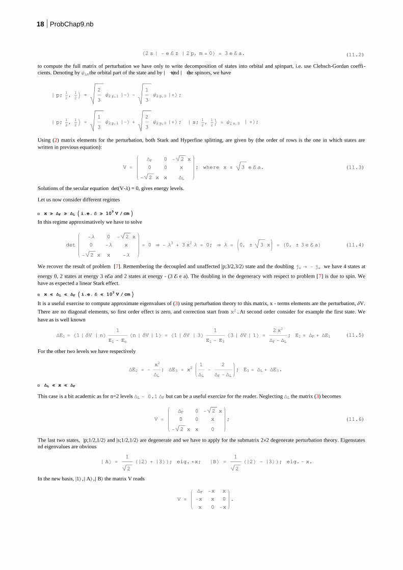
Inthe figure below we present energy levels as a function of x DF, with DL= 0.1 DF. We note that linear Stark effect is quite precocius and start at

about x DF~0.6.

0.2 0.4 0.6 0.8 1.0 1.2 1.4xDF

-2

-1

1

2

3

E

A useful exercise that we leave for the reader is to consider Stark effect as the leading term and fine structure as a perturbation, i.e. compute higherorders in (4).

Problem 12

Parabolic coordinates (Ξ, Η, j) are defined by

x = Ξ Η Cos@jD; y = Ξ Η Sin@jD; z =1

2 HΞ - ΗL;

In notebook problems [*] it has been shown that Schrödinger equation for an hydrogen atom is saparable in these coordinates. Study the Lo Surdo -Stark effect in parabolic coordinates. Compute first and second order effects for an arbitrary state.

æ Solution

à The Schrödinger equation

In this notebook we will use atomic units, Ñ = m = |e| = 1.

In notebook [*] the results obtained here are derived within Mathematica and extended to an arbitrary order in perturbation theory.

In notebook [*] the Schrödinger equation for a coulombic potential has been solved in parabolic coordinates. We report here the basic connectionformulae between cartesian and parabolic coordinates and the for of the laplacian:

(12.1)

x = Ξ Η Cos@jD; y = Ξ Η Sin@jD; z =1

2 HΞ - ΗL;

Ξ = r + z; Η = r - z; j = ArcTanByx

F; r =1

2 HΞ + ΗL;

D =4

Ξ + Η

¶

¶Ξ Ξ

¶

¶Ξ+

4

Ξ + Η

¶

¶Η Η

¶

¶Η+

1

Ξ Η

¶2

¶j2.

The range for these coordinates is

0 £ HΞ, Η L £ ¥ ; 0 £ j £ 2 Π

and volume element is

d3 x =

Ξ + Η

4dΞ dΗ dj.

Interaction with an electric field E, directed along z by convention, is decribed by an interacion - e z E = + |e| z E. We put F for the product |e| E a inatomic units (a is the Bohr radius) and write the interaction Hamiltonian as (see eq. (1) )

ProbChap9.nb 19

(12.2)V =F

2 HΞ - ΗL.

Using (1) the Schrödinger equation takes the form:

-1

2

4

Ξ + Η

¶

¶Ξ Ξ

¶

¶Ξ+

4

Ξ + Η

¶

¶Η Η

¶

¶Η+

1

Ξ Η

¶2

¶j2 Ψ -

2 Z

Ξ + Η Ψ +

F

2 HΞ - ΗL Ψ = E Ψ.

or

(12.3)¶

¶Ξ Ξ

¶

¶Ξ+

¶

¶Η Η

¶

¶Η+

Ξ + Η

4 Ξ Η

¶2

¶j2 Ψ + Z -

F

4 IΞ

2- Η

2M +Ξ + Η

2 E Ψ = 0.

The sistem is invariant under rotation around z axis, then one of the "good" quantum numbers will be m, the eigenvalue of Lz. We look for a solution

with separate variables, in the form

(12.4)Ψ = f1@ΞD f2@ΗD Exp@ä m jD.Substitution in (3), after division by Ψ, gives

1

f1

d

d Ξ Ξ

df1

d Ξ-m2

4 Ξ f1 +

E

2 Ξ f1 -

F

4 Ξ

2 f1 +

1

f2

d

d Η Η

df2

d Η-m2

4 Η f2 +

E

2 Η f2 +

F

4 Η2 f2 + Z = 0.

The first term depends only on Ξ, the second only on Η, since their sum is constant there must be two constant Z1 and Z2 such that

(12.5)

d

d Ξ Ξ

df1

d Ξ+

E

2 Ξ -

m2

4 Ξ-

F

4 Ξ

2+ Z1 f1 = 0;

d

d Η Η

df2

d Η+

E

2 Η -

m2

4 Η+

F

4 Η2

+ Z2 f2 = 0;

Z1 + Z2 = Z.

We can simplify a bit these equations by the change of variables

(12.6)Ε = -2 E ; x = Ε Ξ; y = Ε Η; Βi =Zi

Ε; F =

F

Ε3.

(12.7)

d

d x x

df1

d x+ -

1

4 x -

m2

4 x-

F

4 x2 + Β1 f1 = 0;

d

d y y

df2

d y+ -

1

4 y -

m2

4 y+

F

4 y2 + Β2 f2 = 0;

Β1 + Β2 =Z

Ε.

As is apparent from (7) the spectrum depends only on |m|, and, as we know from general arguments, states ±m will be degenerate.

The procedure to find eigenvalues, as in the case E = 0, is the following

1. Find, for each F, eigenvalues Β1, Β2, these will depend parametrically on F.

2. Substitute in the last constraint in (7) and find Ε (i.e. energy) as a function of F.

à Perturbative solution at first order

At zero order the solution of equations (7) has been found in notebook [*]. Normalizability of the solutions impose

(12.8)Β1 = n1 +È m È +1

2; Β2 = n2 +

È m È +1

2; Þ Β1 + Β2 = n1 + n2 + H È m È +1L º n;

then

(12.9)Β1 + Β2 =Z

ΕÞ Ε =

Z

nÞ E = -

1

2 n2

At fixed n, 0 ² |m| ² n-1 and with fixed n and m, one of the two numbers, e.g. n1, can vary as 0 ² n1² n - |m| - 1, the other being fixed by (8).

Normalized eigenfunctions are given by

(12.10)

20 ProbChap9.nb

(12.10)

fni,m@xD =n!

Hn + È m ÈL!xÈmÈ2 ExpB-

x

2F Ln

ÈmÈ HxL º cni,m xÈmÈ2 ExpB-

x

2F Ln

ÈmÈ HxL

à0

¥

fn1,m fn2,m âx = ∆n1 n2.

We will comment below on the normalization coefficients.

The perturbative calculation is done independently on the two equations in (7), each of them is a kind of Schrödinger equation in which Βi has the

role of energy eigenvalue. It is sufficient to do coputations for Β1, the other one is obtained by F® - F.

To compute perturbative corrections we need matrix elements of x2. We start from recursive relation

(12.11)x LnmHxL = -Hn + mL Ln-1

m HxL - Hn + 1L Ln+1m HxL + H2 n + m + 1L Ln

mHxL.Denoting the diagonal matrix element by X fn È x^2 È fn\,using (11) to right and left functions, and inserting normalization coefficients, we have

immediately (by orthogonality and omitting the fixed index m):

(12.12)Yfn É x2 É fn] =cn2

cn+12

Hn + 1L2 +cn2

cn-12

Hn + mL2 + H2 n + m + 1L = 6 n2 + 6 n Hm + 1L + Hm + 1L Hm + 2L.Up to first order then

Β1 = n1 +È m È +1

2+

F

4 I 6 n1

2+ 6 n1 Hm + 1L + Hm + 1L Hm + 2L M;

Β2 = n2 +È m È +1

2+

F

4 I 6 n2

2+ 6 n2 Hm + 1L + Hm + 1L Hm + 2L M.

and, see the definition of n in (8):

(12.13)Β1 + Β2 = n + F3

2 In12 - n2

2M +3

2 Hn1 - n2L Hm + 1L = n +

3

2F Hn1 - n2L n.

Imposing the constraint (7) , using F = F Ε3 and the zeroth order result Ε = Z/n

Z

Ε= n +

3

2

F

Ε3Hn1 - n2L n > n +

3

2

F

Z3Hn1 - n2L n4 Þ

Ε

Z>

1

n 1 -

3

2

F

Z3Hn1 - n2L n3 Þ Ε >

Z

n-

3

2 F

n

Z

2

Hn1 - n2L,and finally for energy, E = - Ε2/2

(12.14)E = -1

2 Z2

n2+

3

2 F

n

Z Hn1 - n2L.

This gives the first order Stark effect on all levels. It is easy to check low level to compare with more elementary results (prob. [7] ), we considerhydrogen, Z=1:

n = 1; m = 0; Hn1, n2L = 0 Þ ∆E = 0;n = 2; m = 0; Hn1, n2L = H1, 0L, H0, 1L Þ ∆E = ¡3 F ;n = 2; m = ±1; Hn1, n2L = H0, 0L, H0, 1L Þ ∆E = 0 ;

We have the known Stark effect on level n = 2, to compare with problem [7] use F = e E a.

ã The normalization of wave functions

The eigenfunctions (10) are a complete and orthonormal set with respect the measure dx. The eigenfunctions used in notebook [*] where similar butnot identical. In Ξ variable they were

(12.15)

Ψn1 n2 m@Ξ, Η, jD := fn1 m@ΞD fn2 m@ΗD ãä m j

2 Π

;

fn1 m@ΞD = 214 ¶

n!

Hn + È m ÈL!H¶ ΞLÈmÈ2

ã- ¶ Ξ2

LnÈmÈH¶ ΞL

Functions (15) are orthogonal with respect the three dimensional measure induced by parabolic coordinates, i.e.

ProbChap9.nb 21

à Ψn1 n2 m * Ψk1 k2 m' Ξ + Η

4 âΞ dΗ dj = ∆n1 k1 ∆n2 k2 ∆m m'

Functions (15) are not a complete set with respect to this measure, we clearly miss continuum spectrum. In this problem eigenfunctions (10) are used

to solve the auxiliary problem (7). For negative energies we look at real eigenvalues Βiand in this framework (at F = 0 ) functions (10) are a complete

set. If we make the change of variables

f@xD = x-12 g@xD

the first equation (7) becomes

d2

dx2

g@xD +1

4 x2-1

4 x -

m2

4 x-

F

4 x2 + Β1 g@xD,

i.e. a "usual" one dimensional Schrödinger equation with potential

2 V@xD =1

4x +

m2

4 x-

1

4 x2+

F

4 x2

and have only a bound spectrum for F ³ 0. For F = 0 both equations (7) admit only a discrete spectrum, the continuous spectrum of the coulombpotential comes from E > 0 and Ε imaginary. The constraint in this case force to look for imaginary eigenvalues.

When F ­ 0 one of the two equations has a potential non bounded below at infinity, for example the second one if F > 0, the energy levels will beinstable for tunneling, this phenomenon will be analysed with WKB methods, but do not concerne us as far as we consider perturbation theory.

à Perturbative solution at second (and third) order

It is not difficult extend the solution to second order, First we write implicitely the correction ΨH1L to wave functions in the two eigenvalue problems

(7)

(12.16)ΨnH1L@xD = â

s

'fs@xD Xfs È V È fn\

Βn - Βs

; V =F

4x2;

then we use the general formulae

(12.17)∆EnH2L

= YΨ0 É V É ΨnH1L], ∆En

H3L= YΨn

H1L É V É ΨnH1L] - ∆En

H1L YΨn

H1L É ΨnH1L].

Iterating recursion relation (11) we obtain

(12.18)x2 Ln

m = Hn + 2L Hn + 1L Ln-2m

- 2 Hn + 1L H2 n + m + 2L Ln-1m

+

H6 nHn + m + 1L + Hm + 2L Hm + 1LL Lnm - 2 Hn + mL Hm + 2 nL Ln+1

m+ Hm + nL Hn + m - 1L Ln+2

m .

Let us call dk(k = -2,..+2 the coefficients of this relation. Using normalization constants ck this relation an be transformed in a recursive relation for

basis functions:

(12.19)x2 fk@xD = âk=-2

2 cn

cn+k

dk fn+k@xD.Using orthogonality of basis functions the first order correction (16) is

(12.20)ΨnH1L@xD =

F

4 âk=-2,k¹0

2 1

ΒnH0L

- Βn+kH0L

cn

cn+k

dk fn+k@xD

Now we have only to insert (20) in (17) and using (12) and orthogonality to perform integrals. The result with F ® - F will give correction to Β2.

Imposing the constraint (7) will give the corrections to enery levels. We report here the final result of this strightforward but tedious computation

(12.21)

E = -Z2

2 n2+

3

2 F

n

Z Hn1 - n2L -

1

16 F2

n

Z

4A17 n2 - 3 Hn1 - n2L2 - 9 m2 + 19E +

+3

32 F3

n

Z

7

Hn1 - n2LA23 n2 - Hn1 - n2L2 + 11 m2 + 39E.A method to perform the computation to all orders is given in notebook [**]. in particular for the ground state of hydrogenic atoms (n=1,n1 = n2 = 0, m = 0Lone obtains

E = -Z2

2 n2-

9

4 F2

1

Z4.

From previuos result the polarizability Α follows

22 ProbChap9.nb

Α F = -¶E

¶F=

9

2 F

Z4

which reproduces the known result of hydrogen atom, see problem[**].

Problem 13

Consider electron - electron interaction as a small perturbation in an helium atom. Compute to lowest order the energy of ground state of heliumatom. Compute 3-dimensional Fourier transform for the functions

1

r;

Exp@-Μ rDr

; Exp@-Μ rD;and show how these results can be used to solve the problem.

æ Solution

à Introduction

This problem is intended as an introducion to the next one, prob.[14].

In this problem we will use atomic units. Units for length and energy are

(13.1)aB =Ñ2

m e2HBohr radiusL; EB =

m e4

Ñ2=

e2

aB> 27.2114 eV

In these units the non relativistic Hamiltonian for Helium atom is

(13.2)H = -1

2 D1 -

1

2 D2 -

Z

r1-

Z

r2+

1

È r1 - r2 È º H0 +1

È r1 - r2 È.Suffixes 1,2 refer to the electrons. r1, r2 are their position with respect to nucleus, r1 = r1¤ etc. Z is the nuclear charge, Z = 2 for helium otherwise

we will describe ions of Berillium, Z=3, Boron, Z=4 etc.

In this problem we are considering electron-electron interaction as a perturbation. We do not expect good quantitative results as its order of magni-

tude, e2 aBin usual units, is similar toother terms in the Hamiltonian.

H0is a sum of independent hamiltonians, then its ground state is written at once

(13.3)Y0 Hr1, r2L = Ψ1 s Hr1L Ψ1 s Hr2L; E0 = E1 s + E1 s = -Z2

2 1

1+1

1= - Z2.

à Perturbation

The perturbative contribution to the energy of the ground state is

(13.4)DE = X1s;1sÈ 1

È r1 - r2 È È1s;1s\ = à â3r1 â

3r2 Ψ1 s Hr1L¤2 Ψ1 s Hr2L¤2

È r1 - r2 È .

The most simple and general way to compute integrals like (4) is to use multipole expansion for Coulomb potential:

(13.5)1

È r1 - r2 È = â=0

¥ 1

r>

r<

r>

P@Cos HΓLD;with P Legendre polynomials and

r> = Max@r1, r2D; r< = Min@r1, r2D; r1 ×r2 = r1 r2 Cos@ΓD.In the actual case our distribution are spherically symmetric, only =0 term in the sum survives angular integration and we have, splitting the integral:

(13.6)

DE = à â3r1 â

3r2 Ρ Hr1L 1

r>

Ρ Hr2L =

H4 ΠL2 à0

¥

âr1 r12 Ρ Hr1L

1

r1 à0

r1

Ρ Hr2L r22 âr2 + à

0

¥

âr2 r22 Ρ Hr2L

1

r2 à0

r2

Ρ Hr1L r12 âr1 =

2 H4 ΠL2 à0

¥

âr1 r12 Ρ Hr1L

1

r1 à0

r1

Ρ Hr2L r22 âr2.

Using the known wave functions

ProbChap9.nb 23

Ψ1 s = Y00 R1 s@rD =1

4 Π

2 Z32 Exp@-Z rD.

it is easy to compute

(13.7)DE = 2´5

16 Z =

5

8 Z.

For the energy the prediction is (for Z = 2)

E = - Z2 +5

8 Z ® - 2.75 a.u.; Eexp > - 2.90 a.u.

Usually what is reported is ionization energy, i.e. the energy necessary to extract one electron. After ionization we have a one electron atom, with

energy - Z2 2then ionization energy is defined as (we neglect relativistic corrections)

I = -Z2

2- E0 >

Z2

2-5

8 Z = 0.75 a.u. = 1.5 Ry = 20.41 eV.

to be compared with

Iexp > 0.9035 a.u. = 1.807 Ry = 24.5855 eV.

à Different methods to compute an integral

The multipole expansion (5) is a standard way to compute integrals of the form (4), nevertheless it can be useful to have alternative strings in one'sbow.

ã Electrostatic analogy

The integral (4) is the douvle of an electrostatic self - energy for a charge density Ρ:

DE = 2 U; U =1

2 à â

3r1 â3r2

Ρ Hr1L Ρ Hr2LÈ r1 - r2 È

Let us divide the space in shells of width dr, with charge Ρ(r) 4 Π2dr. The self energy can be obtained by summing potential energy of these shells,

the potential being created by charge inside sphere of radius r. The total charge up to radius r, Q(r) creates a potential Q(r)/r at limiting radius r, henthe self energy is

U = à0

¥

4 Π r2 âr Ρ HrL 1

r Q HrL

Once multiplied by the additional factor of two this expression coincides with (6).

ã Fourier transforms

In this book, as often in Physics literature, the fourier transforms are defined in an asymmetric way:

(13.8)f@xD = à dn k

H2 ΠLn Ff@kD ãä k x; Ff@kD = à dn x Ff@kD ã

-ä k x.

This method is based on two well known facts about Fourier transforms :

(13.9)à dn x f*@xD g@xD = à dn k

H2 ΠLn Ff*@kD Fg@kD; Ff*g@kD = Ff@kD Fg@kD.

For real functions Ff*@kD= Ff@-kD. f*g is the convolution of two functions, i.e.

f*g@xD = à dn y f@x - yD g@yD.Direct application of (9) gives for the integral (4):

(13.10)DE = à dn k

H2 ΠLn FΡ*@kD F1r@kD FΡ@kD.

By direct computation, or by taking the Fourier transforms of the equations

- D1

r= 4 Π ∆

H3L HrL; I- D + Μ

2M ã-Μ r

r= 4 Π ∆

H3L HrL;

we have

24 ProbChap9.nb

F1r@kD =4 Π

k2; FB ã-Μ r

rF@kD =

4 Π

k2 + Μ2.

From the second of these relations follows

F@ã-Μ rD@kD = -

¶

¶ΜFB ã-Μ r

rF@kD =

8 Π Μ

Ik2 + Μ2M2.

In our computation :

Ρ = Ψ1 s¤2 =Z3

Π Exp@-2 Z rD; FΡ@kD = 16

Z4

Ik2 + 4 Z2M2;

and

DE =16

2

H2 ΠL3 4 Π á d3 kZ8

Ik2 + 4 Z2M4 1

k2=

2 ×162

Π à0

¥ Z8

Ik2 + 4 Z2M4 âk =

4

Π Z à

0

¥ 1

Ix2 + 1M4 âx =

5

8Z

The last integral can be computed by method of residues. This use of Fourier transforms may seem complicated but the reader must note that itautomatically transform a doubleintegral like (4) in a simpe integral,like the one just computed.

Problem 14

Let us consider electron - electron interaction as a small perturbation in an helium atom. Compute at lowest order the energy of first excited s stateof helium atom. Discuss how Pauli principle select possible states.

æ Solution

à Introduction

In this notebook we will use atomic units. Units for length and energy are

(14.1)aB =Ñ2

m e2HBohr radiusL; EB =

m e4

Ñ2=

e2

aB> 27.2114 eV

In these units the non relativistic Hamiltonian for Helium atom is

(14.2)H = -1

2 D1 -

1

2 D2 -

Z

r1-

Z

r2+

1

È r1 - r2 È º H0 +1

È r1 - r2 È.Suffixes 1,2 refer to the electrons. r1, r2 are their position with respect to nucleus, r1 = r1¤ etc. Z is the nuclear charge, Z = 2 for helium otherwise

we will describe ions of Berillium, Z=3, Boron, Z=4 etc.

In this problem we are considering electron-electron interaction as a perturbation. We do not expect good quantitative results as its order of magni-

tude, e2 aBin usual units, is similar toother terms in the Hamiltonian, but the perturbative computations will give us some hints on the general

properties of the spectrum.

ã Quantum numbers

We are neglecting spin interacions, albeit as we will see spin enter in the determination of energies. Hamiltonian (2) is invariant under globalrotations, i.e. L and Lzare conserved. L is total angular momentum:

(14.3)L = 1 + 2.

Energy in general will depend on L, and, always neglecting spin and other effects (as Pauli principle) we expect at least a degeneracy 2L+1 for eachlevel. To know how levels are organized we need more dynamical information, this is wy we use perturbation theory.

Hamiltonian H0has a much bigger symmetry, it is symmetric under independent rotations of first and second electron. Each rotation invariance imply

a degeneracy (2+1) then for H0we have at least a degeneracy H2 1 + 1L H2 2 + 1L.In effect we have more degeneracy as H0is symmetric under

the exchange of the two electrons, then given a state with quantum numbers (a,b) (and a­ b) then the state (b,a) will have the same energy. Finally

H0is of coulomb type and the accidental degeneracy typical of hydrogen-like systems is at work, i.e. energies depend only on principal quantum

number and not on , this will be a minor complication.

H0 is a sum of independent hamiltonians then eigenstates and energies are written at once:

(14.4)Yab Hr1, r2L = Ψa Hr1L Ψb Hr2L; Ea,b = Ea + Eb = -Z2

2

1

na2

+1

nb2

.

Ψa, Ψbare one electron states in coulomb potential and a,b the relative quantum numbers, i.e. n, , m.

ProbChap9.nb 25

Ψa, Ψbare one electron states in coulomb potential and a,b the relative quantum numbers, i.e. n, , m.

ã Pauli principle

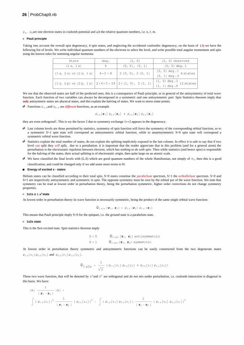
Taking into account the overall spin degeneracy, 4 spin states, and neglecting the accidental coulombic degeneracy, on the basis of (4) we have thefollowing list of levels. We write individual quantum numbers of the electrons to select the level, and write possible total angular momentum and spinusing the known rules for summing angular momenta:

State deg. HL, SL HL, SL observed

H1 s, 1 sL 4 H0, 0L, H0, 1L H0, 0L deg. 1

H1 s, 2 sL or H2 s, 1 sL 42 = 8 2 H0, 0L, 2 H0, 1L H0, 0L deg .1

H0, 1L deg .34 states

H1 s, 2 pL or H2 p, 1 sL 243 = 24 2H1, 0L, 2 H1, 1L H1, 0L deg .3

H1, 1L deg .912 states

We see that the observed states are half of the predicted ones, this is a consequence of Pauli principle, or in general of the antisymmetry of total wavefunction. Each function of two variables can always be decomposed in a symmetric and one antisymmetric part: Spin Statistics theorem imply thatonly antisymetric states are physical states, and this explain the halving of states. We want to stress some points:

Functions Ya,band Yb,a are different functions, as an example

Ψ1 s@r1D Ψ2 s@r2D ¹ Ψ1 s@r2D Ψ2 s@r1Dthey are even orthogonal!. This is wy the factor 2 due to symmetry exchange 1«2 appears in the degeneracy.

Last column levels are those permitted by statistics, symmetry of spin function will force the symmetry of the corresponding orbital function, so toa symmetric S=1 spin state will correspond an antisymmetric orbital function, while to anantisymmetric S=0 spin state will correspond asymmetric orbital wave function.

Statistics explain the total number of states, do not explain the splitting implicitely exposed in the last column. In effect it is safe to say that if twolevel can split they will split, due to a pertubation. it is important that the reader appreciate that in this problem (and for a general atom) theperturbation is the electrostatic repulsion between electron, which has nothing to do with spin. Then while statistics (and hence spin) is responsiblefor the halving of the states, their actual splitting is of electrostatic origin, then quite large on an atomic scale.

We have classified the final levels with (L,S) which are good quantum numbers of the whole Hamiltonian, not simply of H0, then this is a good

classification, and could be changed only if we add some more terms to H.

à Energy of excited s - states

Helium states can be classified according to their total spin, S=0 states constitue the parahelium spectrum, S=1 the orthoHelium spectrum. S=0 andS=1 are respectively antisymmetric and symmetric in spin. The opposite symmetry must be own by the orbital par of the wave function. We note thatsymmetry can be read at lowest order in perturbation theory, being the perturbation symmetric, higher order corrections do not change symmetryproperties.

ã 1s1s º 1 s2state

At lowest order in perturbation theory its wave function is necessarily symmetric, being the product of the same single orbital wave function:

Y1 s1s Hr1, r2L = Ψ1 s Hr1L Ψ1 s Hr2LThis means that Pauli principle imply S=0 for the spinpart, i.e. the ground state is a parahelum state.

ã 1s2s state

This is the first excited state. Spin statistics theorem imply

S = 0 Y1 s2s Hr1, r2L antisymmetric

S = 1 Y1 s2s Hr1, r2L symmetric

At lowest order in perturbation theory symmetric and antisymmetric functions can be easily constructed from the two degenerate states

Ψ1 s@r1DΨ2 s@r2D and Ψ2 s@r1DΨ1 s@r2D.

Y1 s2s =1

2

H Ψ1 s@r1D Ψ2 s@r2D ¡ Ψ2 s@r1D Ψ1 s@r2DL

These two wave function, that will be denoted by YAand YS are orthogonal and do not mix under perturbation, i.e. coulomb interaction is diagonal in

this basis. We have:

XAÈ 1

È r1 - r2 È ÈA\ =

à Ψ1 s@r1D¤2 1

È r1 - r2 È Ψ2 s@r2D¤2 - à Ψ1 s@r1D Ψ2 s@r1D¤ 1

È r1 - r2 È Ψ1 s@r2D Ψ2 s@r2D¤2

26 ProbChap9.nb

XSÈ 1

È r1 - r2 È ÈS\ =

à Ψ1 s@r1D¤2 1

È r1 - r2 È Ψ2 s@r2D¤2 + à Ψ1 s@r1D Ψ2 s@r1D¤ 1

È r1 - r2 È Ψ1 s@r2D Ψ2 s@r2D¤2

For obvious reasons the first integral is named direct integral, and will be denoted by K, and the second exchange integral, and will be denoted by J. Kis very similar to the integral met in ground state computation, J determines the splitting between parahelium and orthohelium. We write:

(14.5)XAÈ 1

È r1 - r2 È ÈA\ = K - J; XSÈ 1

È r1 - r2 È ÈS\ = K + J.

K, and J canbe easily computed on the basis built on hydrogenic functions

(14.6)Ψ1 s =1

4 Π

Z32 2 Exp@-Z rD; Ψ2 s =1

4 Π

Z32 H2 - ZrL2 2

Exp@-Z r2D;

using multipole expansion, already seen in problem [13]:

(14.7)1

È r1 - r2 È = â=0

¥ 1

r>

r<

r>

P@Cos HΓLD;An easy computation gives

(14.8)K =17 Z

81; J =

16 Z

729

Then, at first order in perturbation theory (we report also approximate experimental data):

E@1 s2s; S = 0D = -Z2

2 1 +

1

4+ HK + JL = -

5

8 Z2 +

169

729 Z > - 2.036 a.u.; exp : -2.14577 a.u.

E@1 s2s; S = 1D = -Z2

2 1 +

1

4+ HK - JL = -

5

8 Z2 +

137

729 Z > - 2.124 a.u.; exp : -2.17503 a.u.

E@1 s2s; S = 0D - E@1 s2s; S = 1D =32 Z

729> 0.088 a.u.; exp : 0.02926 a.u.

We see that while ordering of levels is correct, energy differences are badly reproduced.

à Hystorical remarks

It would be very difficult to overemphasize the imprtance of the problem of Helium atom in Quantum Mechanics.

The disagreement between theory and experiment for highly excited Helium states marked the end of old quantum theory. In the words of Born[1], who carried the calculations with Heisenberg:

We may therefore conclude that the systematic application of the principles of the quantum theory .... gives results in agreement with experiment only in those cases where the motion of a single electron is considered; it fails even in the tratment of the motion of two electrons in the helium atom.

In two seminal papers on helium atom [2] Heisenberg put forward the idea of the connection between spin and symmetry of the wave function,idea almost simultaneously advanced by Dirac. The observation is that if one work on unperturbed functions, and without knowing about spinstatistics connection, one should treat electrostatic interaction as a perturbation on a a degenerate level. In the basis

Ψ1 s@r1D Ψ2 s@r2D,Ψ1 s@r2D Ψ2 s@r1D the matrix willbe written as

HI = K K J

J KO

and we know that eigenvalues are K ± J, while eigenfunctions are symmetric and antisymmetric combinations. This structure agree with experimentalknown helium spectrum, whose spin can be detected by interaction with a magnetic field. In the second paper Heisenberg elaborate a quite sophisti-cated form of perturbation theory trying to explain in the new Quantum Mechanics what Old Quantum Theory was enable to explain.

The definitive word on the argument was given by Hylleraas [3], were a variational technique were developed and a spectacular agreement withexperimental data was found. We will study later variational comptations.

The reader who want to go deeper in some of these aspects is referred to the book of Bethe and Salpeter [4].

æ References

[1] M. Born : Vorlesungen uÐber Atommechanik, Springer Verlag, Berlin, 1925; english translation: Mechanics of the Atom, Bell, london, 1927

[2] W. Heisenberg: Z. Physik, 38 (1926) 411 and 39 (1926) 499.

[3] E.A. Hylleraas: Z. Physik, 54, (1929) 347.

[4] H.A. Bethe, E.E. Salpeter: Quantum Mechanics of One-And Two-Electron Atoms, Plenum Publishing Corporation; (1977)

Problem 15

ProbChap9.nb 27