ROBUST PRECONDITIONING FOR XFEM APPLIED TO · ROBUST PRECONDITIONING FOR XFEM APPLIED TO...
22
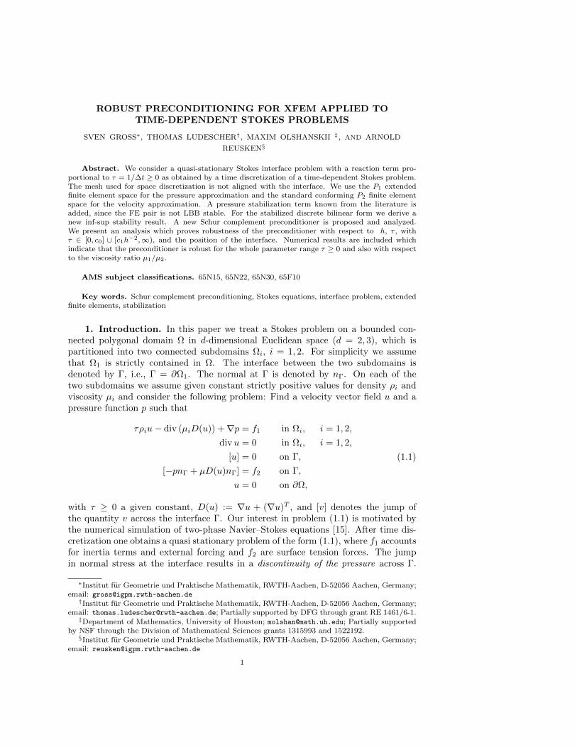
ROBUST PRECONDITIONING FOR XFEM APPLIED TO TIME-DEPENDENT STOKES PROBLEMS SVEN GROSS * , THOMAS LUDESCHER † , MAXIM OLSHANSKII ‡ , AND ARNOLD REUSKEN § Abstract. We consider a quasi-stationary Stokes interface problem with a reaction term pro- portional to τ =1/Δt ≥ 0 as obtained by a time discretization of a time-dependent Stokes problem. The mesh used for space discretization is not aligned with the interface. We use the P 1 extended finite element space for the pressure approximation and the standard conforming P 2 finite element space for the velocity approximation. A pressure stabilization term known from the literature is added, since the FE pair is not LBB stable. For the stabilized discrete bilinear form we derive a new inf-sup stability result. A new Schur complement preconditioner is proposed and analyzed. We present an analysis which proves robustness of the preconditioner with respect to h, τ , with τ ∈ [0,c 0 ] ∪ [c 1 h -2 , ∞), and the position of the interface. Numerical results are included which indicate that the preconditioner is robust for the whole parameter range τ ≥ 0 and also with respect to the viscosity ratio μ 1 /μ 2 . AMS subject classifications. 65N15, 65N22, 65N30, 65F10 Key words. Schur complement preconditioning, Stokes equations, interface problem, extended finite elements, stabilization 1. Introduction. In this paper we treat a Stokes problem on a bounded con- nected polygonal domain Ω in d-dimensional Euclidean space (d =2, 3), which is partitioned into two connected subdomains Ω i , i =1, 2. For simplicity we assume that Ω 1 is strictly contained in Ω. The interface between the two subdomains is denoted by Γ, i.e., Γ = ∂ Ω 1 . The normal at Γ is denoted by n Γ . On each of the two subdomains we assume given constant strictly positive values for density ρ i and viscosity μ i and consider the following problem: Find a velocity vector field u and a pressure function p such that τρ i u - div (μ i D(u)) + ∇p = f 1 in Ω i , i =1, 2, div u =0 in Ω i , i =1, 2, [u]=0 on Γ, [-pn Γ + μD(u)n Γ ]= f 2 on Γ, u =0 on ∂ Ω, (1.1) with τ ≥ 0 a given constant, D(u) := ∇u +(∇u) T , and [v] denotes the jump of the quantity v across the interface Γ. Our interest in problem (1.1) is motivated by the numerical simulation of two-phase Navier–Stokes equations [15]. After time dis- cretization one obtains a quasi stationary problem of the form (1.1), where f 1 accounts for inertia terms and external forcing and f 2 are surface tension forces. The jump in normal stress at the interface results in a discontinuity of the pressure across Γ. * Institut f¨ ur Geometrie und Praktische Mathematik, RWTH-Aachen, D-52056 Aachen, Germany; email: [email protected] † Institut f¨ ur Geometrie und Praktische Mathematik, RWTH-Aachen, D-52056 Aachen, Germany; email: [email protected]; Partially supported by DFG through grant RE 1461/6-1. ‡ Department of Mathematics, University of Houston; [email protected]; Partially supported by NSF through the Division of Mathematical Sciences grants 1315993 and 1522192. § Institut f¨ ur Geometrie und Praktische Mathematik, RWTH-Aachen, D-52056 Aachen, Germany; email: [email protected] 1
Transcript of ROBUST PRECONDITIONING FOR XFEM APPLIED TO · ROBUST PRECONDITIONING FOR XFEM APPLIED TO...
ROBUST PRECONDITIONING FOR XFEM APPLIED TOTIME-DEPENDENT STOKES PROBLEMS
SVEN GROSS∗, THOMAS LUDESCHER† , MAXIM OLSHANSKII ‡ , AND ARNOLD
REUSKEN§
Abstract. We consider a quasi-stationary Stokes interface problem with a reaction term pro-portional to τ = 1/∆t ≥ 0 as obtained by a time discretization of a time-dependent Stokes problem.The mesh used for space discretization is not aligned with the interface. We use the P1 extendedfinite element space for the pressure approximation and the standard conforming P2 finite elementspace for the velocity approximation. A pressure stabilization term known from the literature isadded, since the FE pair is not LBB stable. For the stabilized discrete bilinear form we derive anew inf-sup stability result. A new Schur complement preconditioner is proposed and analyzed.We present an analysis which proves robustness of the preconditioner with respect to h, τ , withτ ∈ [0, c0] ∪ [c1h−2,∞), and the position of the interface. Numerical results are included whichindicate that the preconditioner is robust for the whole parameter range τ ≥ 0 and also with respectto the viscosity ratio µ1/µ2.
AMS subject classifications. 65N15, 65N22, 65N30, 65F10
Key words. Schur complement preconditioning, Stokes equations, interface problem, extendedfinite elements, stabilization
1. Introduction. In this paper we treat a Stokes problem on a bounded con-nected polygonal domain Ω in d-dimensional Euclidean space (d = 2, 3), which ispartitioned into two connected subdomains Ωi, i = 1, 2. For simplicity we assumethat Ω1 is strictly contained in Ω. The interface between the two subdomains isdenoted by Γ, i.e., Γ = ∂Ω1. The normal at Γ is denoted by nΓ. On each of thetwo subdomains we assume given constant strictly positive values for density ρi andviscosity µi and consider the following problem: Find a velocity vector field u and apressure function p such that
τρiu− div (µiD(u)) +∇p = f1 in Ωi, i = 1, 2,
div u = 0 in Ωi, i = 1, 2,
[u] = 0 on Γ,
[−pnΓ + µD(u)nΓ] = f2 on Γ,
u = 0 on ∂Ω,
(1.1)
with τ ≥ 0 a given constant, D(u) := ∇u + (∇u)T , and [v] denotes the jump ofthe quantity v across the interface Γ. Our interest in problem (1.1) is motivated bythe numerical simulation of two-phase Navier–Stokes equations [15]. After time dis-cretization one obtains a quasi stationary problem of the form (1.1), where f1 accountsfor inertia terms and external forcing and f2 are surface tension forces. The jumpin normal stress at the interface results in a discontinuity of the pressure across Γ.
∗Institut fur Geometrie und Praktische Mathematik, RWTH-Aachen, D-52056 Aachen, Germany;email: [email protected]†Institut fur Geometrie und Praktische Mathematik, RWTH-Aachen, D-52056 Aachen, Germany;
email: [email protected]; Partially supported by DFG through grant RE 1461/6-1.‡Department of Mathematics, University of Houston; [email protected]; Partially supported
by NSF through the Division of Mathematical Sciences grants 1315993 and 1522192.§Institut fur Geometrie und Praktische Mathematik, RWTH-Aachen, D-52056 Aachen, Germany;
email: [email protected]
1
Below we shall introduce a well-posed weak formulation of this problem, in which thecondition [u] = 0 is treated as an essential condition in the choice of the trial spaceand the condition on the normal stresses is treated as a natural interface condition. Intwo-phase flow applications the interface is unknown and finding its location is a partof the numerical simulation. Thus often the fluid dynamics problem is coupled withan interface capturing technique. One commonly used interface capturing techniqueis the level set method, see [28, 8, 24] and the references therein. If the level setmethod is used, then typically in the discretization of the flow equations the interfaceis not aligned with the grid. This causes certain difficulties with respect to an accu-rate discretization of the flow variables. Recently, extended finite element techniques(XFEM) have been developed to obtain accurate finite element discretizations, see,for example, [10, 17, 15, 7]. These methods are closely related to so-called CutFEM,cf. [5]. We consider one particular XFEM, in which the pressure variable is approxi-mated in a conforming P1-XFE space and the velocity is approximated in the standardconforming P2-FE space. This pair of spaces is popular in the discretization of two-phase incompressible flows [13, 25, 26]. The pair is not LBB stable and therefore astabilization technique is needed. We use the stabilization suggested in [17]. In therecent report [18], this finite element discretization method has been analyzed for thestationary variant of (1.1), i.e., τ = 0. For the corresponding variational formulation,an inf-sup stability result is derived with the key property that the stability constantis uniform with respect to h, the viscosity quotient µ1/µ2 and the position of the in-terface in the triangulation. Based on this result and interpolation error estimates,optimal discretization error bounds are derived in [18]. We use this discretizationfor the quasi stationary problem (1.1). After discretization one obtains a symmetricsaddle point system. Due to the use of the standard P2-FE space for the velocity,optimal preconditioners for the velocity block in the stiffness matrix are known (e.g.,multigrid). In [18] a robust Schur complement preconditioner for the stationary case(τ = 0) is presented. In this paper, we derive a new Schur complement preconditionerfor the quasi-stationary case (τ ≥ 0). We propose a preconditioner that is robust withrespect to h, τ , µ1/µ2 and the position of the interface in the triangulation.The three main contributions of this paper are the following ones. Firstly, we presenta Schur complement preconditioner that is new. Secondly, for a part of the parameterrange, namely τ ∈ [0, c0] ∪ [c1h
−2,∞), with constants ci > 0, we give a theoreticalanalysis from which the robustness property follows. For our analysis, we need an LBBtype stability result for the Darcy limit, i.e. τ →∞. We prove this new result (3.2).Finally, we give results of systematic numerical experiments, which indicate that therobustness property of the preconditioner holds for the whole parameter range τ ≥ 0,and propose a slight modification of the Schur complement preconditioner which hasimproved robustness with respect to the density ratio ρ1/ρ2.
2. Discrete problem: P2-P1XFEM pair. For the finite element method wefirst introduce a suitable weak formulation of (1.1). For a subdomain ω of Ω the L2
scalar product on ω is denoted by (·, ·)0,ω. We use the notation (·, ·)0 := (·, ·)0,Ω. Thepiecewise constant functions µ, ρ are defined by µ(x) = µi, ρ(x) = ρi for x ∈ Ωi. Weintroduce the spaces V := H1
0 (Ω)d, Q := p ∈ L2(Ω) |∫
Ωµ−1p(x) dx = 0 and the
bilinear forms
a(u, v) :=1
2
∫Ω
µD(u) : D(v) dx, b(v, p) = −(div v, p)0.
2
The weak formulation reads as follows: Given f ∈ V ′ find (u, p) ∈ V ×Q such thata(u, v) + τ(ρu, v)0 + b(v, p) = f(v) for all v ∈ V,
b(u, q) = 0 for all q ∈ Q. (2.1)
The functional f contains contributions from both the volume force f1 and the surfaceforce f2 in (1.1). We refer to the literature for a derivation of this weak formulation,which is well-posed [11, 15].
Assume a family of shape regular quasi-uniform triangulations consisting of sim-plices Thh>0. The triangulations are not fitted to the interface Γ. Correspondingto the family of triangulations, we assume a family of discrete surfaces Γhh>0 ap-proximating Γ. Each Γh is a C0,1 surface and can be partitioned in planar segments(line segments for d = 2, triangles or quadrilaterals for d = 3), consistent with theouter triangulation Th, i.e. for any T ∈ Th an intersection T ∩ Γh is either planar orhas zero (d− 1)-measure. We assume that Γh is close to Γ in the following sense:
ess supx∈Γh
|n(x)− nh(x)| ≤ c h, (2.2)
where n is the extension of nΓ in a neighborhood of Γ and nh is a unit normal onΓh. Since the rest of the paper deals with a discrete problem, in what follows andwithout ambiguity, Ω1 and Ω2 denote the interior and the exterior of Γh rather thanof Γ. The coefficients ρi, µi are assumed to be piecewise constant with respect to thismesh-dependent partition Ω on Ω1 and Ω2.
We introduce the subdomains
Ωi,h := T ∈ Th | measd(T ∩ Ωi) > 0 , i = 1, 2,
and the corresponding standard linear finite element spaces
Qi,h := vh ∈ C(Ωi,h) | vh|T ∈ P1 ∀ T ∈ Ωi,h , i = 1, 2.
We use the same notation Ωi,h for the set of simplices as well as for the subdomainof Ω which is formed by these simplices, as its meaning is clear from the context. Forthe stabilization procedure that is introduced below we need a further partitioning ofΩi,h. Define the set of elements intersected by Γh:
T Γh := T ∈ Th | measd−1(T ∩ Γh) > 0 ,
and let
ωi,h := Ωi,h \ T Γh , i = 1, 2.
Note that Th = ω1,h ∪ω2,h ∪T Γh holds and forms a disjoint union. The corresponding
sets of faces (needed in the stabilization procedure) are given by
Fi = F ⊂ ∂T | T ∈ T Γh , F 6⊂ ∂Ωi,h , i = 1, 2,
and Fh := F1 ∪ F2. For each F ∈ Fh a fixed orientation of its normal is chosenand the unit normal with that orientation is denoted by nF . These definitions areillustrated, for d = 2, in Fig. 2.1.
3
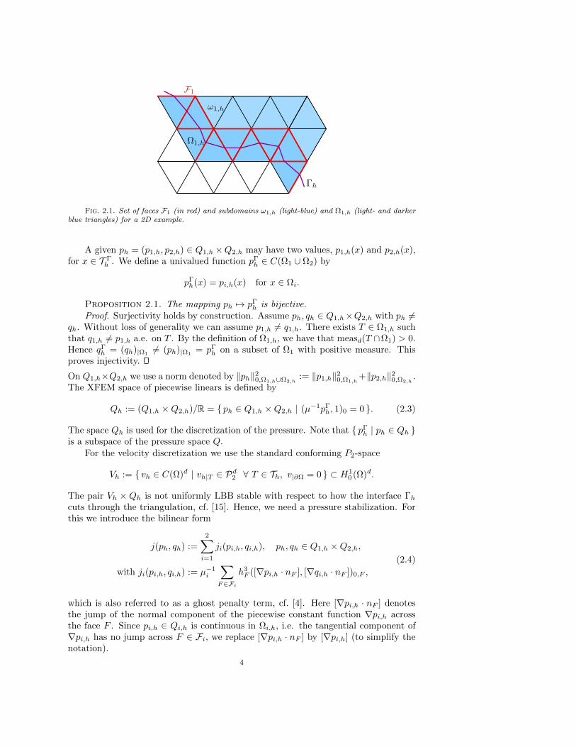
Γh
ω1,h
Ω1,h
F1
Fig. 2.1. Set of faces F1 (in red) and subdomains ω1,h (light-blue) and Ω1,h (light- and darkerblue triangles) for a 2D example.
A given ph = (p1,h, p2,h) ∈ Q1,h ×Q2,h may have two values, p1,h(x) and p2,h(x),for x ∈ T Γ
h . We define a univalued function pΓh ∈ C(Ω1 ∪ Ω2) by
pΓh(x) = pi,h(x) for x ∈ Ωi.
Proposition 2.1. The mapping ph 7→ pΓh is bijective.
Proof. Surjectivity holds by construction. Assume ph, qh ∈ Q1,h×Q2,h with ph 6=qh. Without loss of generality we can assume p1,h 6= q1,h. There exists T ∈ Ω1,h suchthat q1,h 6= p1,h a.e. on T . By the definition of Ω1,h, we have that measd(T ∩Ω1) > 0.Hence qΓ
h = (qh)|Ω16= (ph)|Ω1
= pΓh on a subset of Ω1 with positive measure. This
proves injectivity.
On Q1,h×Q2,h we use a norm denoted by ‖ph‖20,Ω1,h∪Ω2,h:= ‖p1,h‖20,Ω1,h
+‖p2,h‖20,Ω2,h.
The XFEM space of piecewise linears is defined by
Qh := (Q1,h ×Q2,h)/R = ph ∈ Q1,h ×Q2,h | (µ−1pΓh, 1)0 = 0 . (2.3)
The space Qh is used for the discretization of the pressure. Note that pΓh | ph ∈ Qh
is a subspace of the pressure space Q.For the velocity discretization we use the standard conforming P2-space
Vh := vh ∈ C(Ω)d | vh|T ∈ Pd2 ∀ T ∈ Th, v|∂Ω = 0 ⊂ H10 (Ω)d.
The pair Vh × Qh is not uniformly LBB stable with respect to how the interface Γhcuts through the triangulation, cf. [15]. Hence, we need a pressure stabilization. Forthis we introduce the bilinear form
j(ph, qh) :=
2∑i=1
ji(pi,h, qi,h), ph, qh ∈ Q1,h ×Q2,h,
with ji(pi,h, qi,h) := µ−1i
∑F∈Fi
h3F ([∇pi,h · nF ], [∇qi,h · nF ])0,F ,
(2.4)
which is also referred to as a ghost penalty term, cf. [4]. Here [∇pi,h · nF ] denotesthe jump of the normal component of the piecewise constant function ∇pi,h acrossthe face F . Since pi,h ∈ Qi,h is continuous in Ωi,h, i.e. the tangential component of∇pi,h has no jump across F ∈ Fi, we replace [∇pi,h · nF ] by [∇pi,h] (to simplify thenotation).
4
The discretization of (2.1) that we consider is as follows: determine (uh, ph) ∈Vh ×Qh such that
k((uh, ph), (vh, qh)
)= f(vh) for all (vh, qh) ∈ Vh ×Qh, (2.5)
k((uh, ph), (vh, qh)
):= a(uh, vh) + b(vh, p
Γh) + τ(ρuh, vh)0 + b(uh, q
Γh)− εpj(ph, qh),
with a sufficiently large stabilization parameter εp ≥ 0, independent of τ , h, and howΓh intersects the mesh. In [18] this finite element discretization method was analyzedfor the stationary case, i.e. τ = 0. A uniform LBB type stability result and optimalorder error estimates were derived. In this paper, we prove a different uniform inf-supstability result for the pair of finite element spaces and, based on this result, we focuson developing a robust preconditioner for the algebraic problem.
3. LBB type stability conditions. In [18] the following LBB type inequalitywas derived:
supvh∈Vh
(div vh, pΓh)0
‖µ 12∇vh‖0
+
(2∑i=1
∑F∈Fi
h3‖µ−12
i [∇pi,h]‖20,F
) 12
& ‖µ− 12 ph‖0,Ω1,h∪Ω2,h
, (3.1)
for all ph ∈ Qh. This result forms the basis for the analysis of the Schur complementpreconditioner for the case τ = 0 in [18]. Here and in the remainder of this paper weuse the notation A & B, when A ≥ cB holds with a positive constant c independent ofh, the problem parameters ρ, µ, and of how Γh intersects the triangulation. Similarly,A . B is defined and A ' B obviously means that both A & B and A . B hold.The goal of this section is to prove the alternative LBB type stability property
supvh∈Vh
(div vh, pΓh)0
‖ρ 12 vh‖0
+
(2∑i=1
∑F∈Fi
h‖ρ−12
i [∇pi,h]‖20,F
) 12
& ‖ρ− 12∇pΓ
h‖0,Ω1∪Ω2 + ρ− 1
2maxh
− 12 ‖[pΓ
h]‖0,Γh∀ ph ∈ Q1,h ×Q2,h, (3.2)
where [pΓh] := (p1,h−p2,h)|Γh
denotes the interfacial jump of pΓh and ρmax = maxρ1, ρ2.
Recall that the P2-P1XFEM pair (Vh, Qh) is not LBB stable. The second term onthe left hand side is a ghost penalty stabilization as in (2.4), however, with a differenth-scaling. We split the proof of (3.2) into two partial results in the next two lemmata.
Lemma 3.1. The following uniform bound holds for i = 1, 2:
supvh ∈ Vh
supp(vh) ⊂ Ωi
(div vh, pΓh)0
‖vh‖0+
(∑F∈Fi
h‖[∇pi,h]‖20,F
) 12
& ‖∇pΓh‖0,Ωi
∀ ph ∈ Qi,h.
(3.3)
Proof. For any two tetrahedra T1, T2 ∈ Ωi,h sharing a face F , the regularity oftriangulation assumption yields the estimate
‖∇pi,h‖20,T1. ‖∇pi,h‖20,T2
+ h‖[∇pi,h]‖20,F .
Applying the above inequality to estimate ‖∇pi,h‖20,T over all T ∈ T Γh , and using the
fact that any T ∈ T Γh can be reached starting from a suitable tetrahedron in ωi,h
crossing a finite independent of h number of faces from Fi, we obtain the estimate∑F∈Fi
h‖[∇pi,h]‖20,F + ‖∇pi,h‖20,ωi,h≥ c ‖∇pi,h‖20,Ωi,h
≥ c0‖∇pΓh‖20,Ωi
. (3.4)
5
(This estimate was introduced in the analysis of a stabilized Nitsche method for thePoisson and Stokes equations in [6, 22].) Let Vh(ωi,h) be the velocity FE space on thetriangulation ωi,h ⊂ Ωi (zero values on ∂ωi,h). From the literature [3] the followinginf-sup property of the Hood-Taylor P2-P1 pair is known:
supvh∈Vh(ωi,h)
(div vh, pi,h)
‖vh‖0,ωi,h
≥ ci‖∇pi,h‖0,ωi,h, ∀ pi,h ∈ Qi,h, (3.5)
with ci > 0 independent of h. We square (3.5), scale with c−2i and combine it with
(3.4) to obtain
c−2i sup
vh∈Vh(ωi,h)
(div vh, pi,h)2
‖vh‖20,ωi,h
+∑F∈Fi
h‖[∇pi,h]‖20,F ≥ c0‖∇pΓh‖20,Ωi
.
Simple calculations yield (3.3).
We need to derive a uniform bound for the second term on the right-hand side of (3.2).This is done in Lemma 3.2. For the proof of that lemma we need some special decom-position of the surface Γh, that we now introduce. We start with the decompositionof Γh into the set of (planar) segments FΓ := F := Γh ∩ T | T ∈ T Γ
h :
Γh =⋃
F∈FΓ
F.
A subset of “large” surface segments is defined by
F0Γ := F ∈ FΓ | measd−1(F ) ≥ γ0h
d−1 ,
with a suitable constant γ0. Proposition 4.2 from [9] implies that there exist constantsγ0 > 0 and c > 0 depending on the shape regularity of the outer triangulation Th,but independent of h and of how Γh intersects the mesh, such that for each F ∈ FΓ
there exists an F 0 ∈ F0Γ satisfying
dist(F, F 0) ≤ c h. (3.6)
For every Γh∩T = F ∈ F0Γ let b(F ) be the barycenter of F and v(F ) ∈ ∂T a vertex
of T that is closest to b(F ). Let φ(F ) be the scalar nodal linear finite element basis
function corresponding to the vertex v(F ). Let F0Γ be a maximal subset of F0
Γ such
that supp(φ(F ))∩supp(φ(F )) = ∅ for any F, F ∈ F0Γ, F 6= F . The property (3.6) also
holds with the set F0Γ replaced by the smaller set F0
Γ (and a possibly larger constant
c). The elements in F0Γ are labeled by an index set K, i.e., F0
Γ = Fk | k ∈ K. Each
F ∈ FΓ \ F0Γ is added to the (or one of the) surface segments Fk ∈ F0
Γ which hassmallest distance to F . The resulting enlarged surface macro elements are denotedby Fk.
This results in a decomposition of Γh with the following propertiesΓh =
⋃k∈K
Fk, int(Fk) ∩ int(Fj) = ∅ if k 6= j,
∀ k ∈ K ∃Fk ∈ F0Γ, such that Fk ⊂ Fk,
|Fk| ' hd−1, diam(Fk) . h for all k ∈ K.6
Lemma 3.2. There exists h0 > 0 such that for all h ≤ h0 the uniform bound
supvh∈Vh
(div vh, pΓh)0
‖vh‖0+
(2∑i=1
∑F∈Fi
h‖[∇pi,h]‖20,F
) 12
& h−12 ‖[pΓ
h]‖0,Γh(3.7)
for all ph ∈ Q1,h ×Q2,h holds.Proof. For a given ph ∈ Q1,h × Q2,h, introduce the notation q = [pΓ
h]. We thushave
h−1‖[pΓh]‖20,Γh
= h−1
∫Γh
q2 dx = h−1∑k∈K
∫Fk
q2 dx.
Let bk = b(Fk) be the barycenter of a large surface element Fk ⊂ Fk (as explainedabove). For x ∈ Fk let
∫ xbk∇q · t ds be the line integral along the shortest path in Fk
which connects bk and x. Here t denotes the tangential unit vector along this path.The domain formed by the simplices in T Γ
h that are intersected by the macro surface
segment Fk is denoted by T Γk . Note that |T Γ
k | ' hd holds. Using this, ‖x− bk‖ . h,and the estimate in (3.4) we get:
h−1∑k∈K
∫Fk
∣∣∣∣∫ x
bk
∇q · t ds∣∣∣∣2 dx . h
∑k∈K|Fk|
2∑i=1
‖∇pi,h‖2L∞(Fk)
. hd∑k∈K
2∑i=1
‖∇pi,h‖2L∞(Fk).∑k∈K
2∑i=1
∫T Γk
|∇pi,h|2 dx
.2∑i=1
‖∇pi,h‖20,Ωi,h.
2∑i=1
‖∇pi,h‖20,ωi+
2∑i=1
∑F∈Fi
h‖[∇pi,h]‖20,F
. ‖∇pΓh‖20,Ω1∪Ω2
+
2∑i=1
∑F∈Fi
h‖[∇pi,h]‖20,F .
(3.8)
Using q(x) = q(bk) +∫ x
bk∇q · t ds we obtain
h−1‖[pΓh]‖20,Γh
≤ 2h−1∑k∈K|Fk| q(bk)2 + 2h−1
∑k∈K
∫Fk
∣∣∣∣∫ x
bk
∇q · t ds∣∣∣∣2 dx
. hd−2∑k∈K
q(bk)2 + ‖∇pΓh‖20,Ω1∪Ω2
+2∑i=1
∑F∈Fi
h‖[∇pi,h]‖20,F
. hd−2∑k∈K
q(bk)2 +
[supvh∈Vh
(div vh, pΓh)0
‖vh‖0
]2
+
2∑i=1
∑F∈Fi
h‖[∇pi,h]‖20,F ,
(3.9)
where in the last inequality we used Lemma 3.1. It remains to derive a bound for thefirst term on the right-hand side of (3.9), which is denoted by
Q := hd−2∑k∈K
q(bk)2.
Recalling that nh denotes the unit normal vector on Γh and vk = v(Fk) for Fk ∈ F0Γ,
Fk ⊂ Fk, we define the velocity piecewise linear finite element function uh ∈ Vh:
uh(x) =
q(bk)nh(bk) if x = vk, k ∈ K0 at all other vertices in T Γ
h .
7
Due to the construction of the set of surface segments F0Γ it follows that uh is a sum
of nodal (vector) basis functions with non-overlapping supports. From the definitionof uh it follows:
Q = hd−2∑k∈K|uh(vk)|2 & h−2‖uh‖20. (3.10)
Furthermore, on Fk we have that x 7→ q(bk)uh(x) · nh(bk) is a scalar piecewise linearnon-negative function and on Fk ⊂ Fk:∫
Fk
q(bk)uh(x) · nh(bk) dx ' |Fk|q(bk)uh(bk) · nh(bk)
' hd−1q(bk)uh(vk) · nh(bk),
(3.11)
where in the second equivalence we used that vk is the closest vertex to bk. Using(3.11) we get
Q = hd−2∑k∈K
q(bk)uh(vk) · nh(bk)
' h−1∑k∈K
∫Fk
q(bk)uh(x) · nh(bk) dx
≤ h−1∑k∈K
∫Fk
q(bk)uh(x) · nh(bk) dx
= h−1∑k∈K
∫Fk
q(x)uh(x) · nh(x) dx
+ h−1∑k∈K
∫Fk
q(bk)uh(x) ·(nh(bk)− nh(x)
)dx
+ h−1∑k∈K
∫Fk
(q(bk)− q(x)
)uh(x) · nh(x) dx
=: h−1
∫Γh
q(x)uh(x) · nh(x) dx+R1 +R2.
(3.12)
We derive a bound for the term R1. Let d be the signed distance function to theC2-smooth surface Γ, hence ∇d(x) = n(x) for x in a neighborhood of Γ. For x ∈ Fkwe get, using (2.2),
‖nh(bk)− nh(x)‖ ≤ ‖nh(bk)−∇d(bk)‖+ ‖∇d(x)− nh(x)‖+ ‖∇d(bk)−∇d(x)‖≤ ch+ ‖D2d‖∞‖bk − x‖ . h.
Hence, noting ‖uh‖L∞(Fk) ≤ |q(bk)|, we obtain
|R1| . h−1∑k∈K|Fk||q(bk)|‖uh‖L∞(Fk)h . hd−1
∑k∈K
q(bk)2 ' hQ. (3.13)
For deriving a bound for R2 we use q(x)−q(bk) =∫ x
bk∇q · t ds and the results in (3.8)
8
and in Lemma 3.1:
|R2| .(h−1
∑k∈K
∫Fk
∣∣ ∫ x
bk
∇q · t ds∣∣2dx) 1
2(h−1
∑k∈K|Fk|‖uh‖2L∞(Fk)
) 12
.(‖∇pΓ
h‖20,Ω1∪Ω2+
2∑i=1
∑F∈Fi
h‖[∇pi,h]‖20,F) 1
2(hd−2
∑k∈K
q(bk)2) 1
2
.
supvh∈Vh
(div vh, pΓh)0
‖vh‖0+
(2∑i=1
∑F∈Fi
h‖[∇pi,h]‖20,F
) 12
√Q.
(3.14)
To handle the first term on the right-hand side of (3.12) we use integration by parts,Lemma 3.1 and (3.10):
h−1
∫Γh
q(x)uh(x) · nh(x) dx =(−div uh, ph)0
‖uh‖0(h−1‖uh‖0
)+ h−1
2∑i=1
∫Ωi
∇pi,h · uh dx
.
(supvh∈Vh
(div vh, ph)0
‖vh‖0+ ‖∇pΓ
h‖0,Ω1∪Ω2
)(h−1‖uh‖0
)(3.15)
.
(supvh∈Vh
(div vh, ph)0
‖vh‖0+( 2∑i=1
∑F∈Fi
h‖[∇pi,h]‖20,F) 1
2
)√Q.
Combination of (3.12)–(3.15) yields, for h ≤ h0 and h0 > 0 sufficiently small,
Q .
[supvh∈Vh
(div vh, ph)0
‖vh‖0
]2
+
2∑i=1
∑F∈Fi
h‖[∇pi,h]‖20,F ,
and using this in (3.9) completes the proof.
The analysis above leads to the main result of this section.Theorem 3.3. There exists h0 > 0 such that for all h ≤ h0 the following uniform
estimate holds:
supvh∈Vh
(div vh, pΓh)0
‖ρ 12 vh‖0
+
(2∑i=1
∑F∈Fi
h‖ρ−12
i [∇pi,h]‖20,F
) 12
& ‖ρ− 12∇pΓ
h‖0,Ω1∪Ω2+ ρ− 1
2maxh
− 12 ‖[pΓ
h]‖0,Γh∀ ph ∈ Q1,h ×Q2,h, (3.16)
Proof. Since the sup in the left part of (3.3) is over finite element velocity functions
with support in Ωi, one can scale (3.3) with ρ− 1
2i and add the results for i = 1, 2, which
yields
supvh∈Vh
(div vh, pΓh)
‖ρ 12 vh‖0
+
(2∑i=1
∑F∈Fi
h‖ρ−12
i [∇pi,h]‖20,F
) 12
&2∑i=1
‖ρ−12
i ∇pΓh‖0,Ωi
= ‖ρ− 12∇pΓ
h‖0,Ω1∪Ω2∀ ph ∈ Q1,h ×Q2,h.
Adding this estimate and the one in (3.7) scaled with ρ− 1
2max proves the theorem.
9
4. Algebraic problem. In this section, we introduce the matrix-vector repre-sentation of the finite element problem (2.5). For Vh we use the standard nodal basisdenoted by (ψj)1≤j≤m, i.e.,
Vh 3 uh =
m∑j=1
xjψj . (4.1)
The vector representation of uh is denoted by x = (x1, . . . , xm)T ∈ Rm. In Qi,h wehave a standard nodal basis denoted by (φi,j)1≤j≤ni , i = 1, 2, i.e.,
Q1,h ×Q2,h 3 ph = (p1,h, p2,h) =( n1∑j=1
y1,jφ1,j ,
n2∑j=1
y2,jφ2,j
). (4.2)
The vector representation of ph is denoted by y = (y1,1, . . . , y1,n1 , y2,1, . . . , y2,n2)T ∈Rn1+n2 . We use 〈·, ·〉 and ‖·‖ for the Euclidean scalar product and norm. The bilinearforms a(·, ·), (ρ·, ·)0, b(·, ·), j(·, ·) have corresponding matrix representations, denotedby A ∈ Rm×m, C ∈ Rm×m, B ∈ R(n1+n2)×m, J ∈ R(n1+n2)×(n1+n2), respectively. Thefollowing holds:
a(uh, uh) = 〈Ax,x〉 for all uh ∈ Vh,(ρuh, uh)0 = 〈Cx,x〉 for all uh ∈ Vh,b(uh, p
Γh) = 〈Bx,y〉 for all uh ∈ Vh, ph ∈ Q1,h ×Q2,h,
j(ph, ph) = 〈Jy,y〉 for all ph ∈ Q1,h ×Q2,h.
The matrices A,C are symmetric positive definite. The matrix J is symmetric positivesemi-definite. Let 1 := (1, . . . , 1)T ∈ Rn1+n2 . From b(uh, 1) = 0 for all uh ∈ Vh andj(1, qh) = 0 for all qh ∈ Q1,h×Q2,h it follows that BT1 = J1 = 0 holds. We introducetwo mass matrices in the pressure space:
M = blockdiag(M1,M2), (Mi)k,l := (µ−1i φi,k, φi,l)0,Ωi,h
, 1 ≤ k, l ≤ ni, i = 1, 2,
M = blockdiag(M1, M2), (Mi)k,l := (µ−1i φi,k, φi,l)0,Ωi
, 1 ≤ k, l ≤ ni, i = 1, 2.
For these mass matrices we have the relations
〈My,y〉 = ‖µ−12
1 p1,h‖20,Ω1,h+ ‖µ−
12
2 p2,h‖20,Ω2,h= ‖µ− 1
2 ph‖20,Ω1,h∪Ω2,h,
〈My,y〉 = ‖µ−12
1 p1,h‖20,Ω1+ ‖µ−
12
2 p2,h‖20,Ω2=
2∑i=1
‖µ−12
i pΓh‖20,Ωi
= ‖µ− 12 pΓh‖20.
The matrix-vector representation of the discrete problem (2.5) is as follows. First
note that (µ−1pΓh, 1)0 = 0 iff 〈My,1〉 = 0. The discrete problem is given by: Find
x ∈ Rm, y ∈ Rn1+n2 with 〈My,1〉 = 0 such that
K
(xy
):=
(A+ τC BT
B −εpJ
)(xy
)=
(b0
), bj = (f, ψj)0, 1 ≤ j ≤ m. (4.3)
The matrix K of the algebraic system (4.3) is symmetric indefinite. One commonapproach to solve the system numerically is to exploit the structure of the matrix andto apply a Krylov subspace method with block diagonal preconditioner:
K :=
(Aτ 00 Qτ
),
10
where Aτ , Qτ are both SPD matrices and should be chosen as preconditioners of the(1,1)-block A+ τC and the Schur complement of K, which is given by
Sτ := B(A+ τC)−1BT + εpJ. (4.4)
We refer to [2] for a review of this and other approaches to the numerical solution ofsaddle point algebraic systems. It is well-known that if Aτ is uniformly (with respectto the relevant parameters) spectrally equivalent to A + τC and Qτ is uniformlyspectrally equivalent to Sτ , a preconditioned MINRES method, with preconditionerK, applied to the system (4.3) has a high rate of convergence for the whole parameterrange. Good preconditioners Aτ for A+ τC are known, e.g. a multigrid method. Inthe next section we introduce a Schur complement preconditioner Qτ .
5. Schur complement preconditioner. In this section we introduce a precon-ditioner for the Schur complement Sτ .
An ansatz for the Schur complement preconditioner is obtained by looking at thecontinuous level. It is known that for the Schur complement corresponding to theweak formulation (2.1), with µ1 = µ2 = ρ1 = ρ2 = 1, a uniform preconditioner (withrespect to τ) is given by
Q−1τ := I − τ∆−1
N , (5.1)
cf. [23, 19, 21]. Here ∆−1N is the solution operator of the following Neumann problem:
given f ∈ L20(Ω), determine p ∈ H1(Ω) ∩ L2
0(Ω) such that
(∇p,∇q)0 = (f, q)0 for all q ∈ H1(Ω). (5.2)
The preconditioner (5.1) interpolates between two extreme cases τ = 0 (the Schurcomplement preconditioner for the stationary Stokes problem) and τ →∞ (the pres-sure Poisson problem). We shall use the same interpolation idea on the discrete leveland for variable coefficients.
For τ = 0, it is shown in [18] that the preconditioner Q0 := M + εpJ is spectrallyequivalent to S0, i.e. Q0 ' S0, with spectral constants independent of h, µ, and ofhow Γ intersects the triangulation (note that ρ occurs in neither Q0 nor S0).
For the other extreme case, τ → ∞, a preconditioner for Sτ is constructed byusing a suitable discrete version of the Neumann problem (5.2) with variable diffusioncoefficient: Determine p ∈ H2(Ω1 ∪ Ω2) ∩ L2
0(Ω) such that
−div ρ−1∇p = f in Ωi, i = 1, 2,
[ρ−1∇p · n] = 0 on Γ,
[p] = 0 on Γ,
∇p · n∂Ω = 0 on ∂Ω.
(5.3)
A convergent second order accurate discretization in the XFEM space is obtainedby enforcing weak continuity at the interface using the Nitsche method. This dis-cretization was introduced and analyzed in [16]. We recall some results from thatpaper. One defines the Nitsche-XFEM discretization of the Neumann problem (5.3)as follows: Find ph ∈ Qh such that
(ρ−1∇ph,∇qh)0,Ω1∪Ω2− (ρ−1∇ph · n, [qh])0,Γh
− (ρ−1∇qh · n, [ph])0,Γh
+ λh−1ρ−1min[ph], [qh])0,Γh
= (f, qh)0 for all qh ∈ Qh.(5.4)
11
Here we used the average w := κ1w1 + κ2w2 with element-wise constants κi =
κi(T ) = |Ωi∩T ||T | for T ∈ T Γ
h , ρmin = minρ1, ρ2. The parameter λ > 0 is needed for
stabilization. The bilinear form for this discrete problem is given by
sh(ph, qh) := (ρ−1∇ph,∇qh)0,Ω1∪Ω2− (ρ−1∇ph · n, [qh])0,Γh
− (ρ−1∇qh · n, [ph])0,Γh+ λh−1ρ−1
min([ph], [qh])0,Γh.
(5.5)
It is known that this bilinear form is uniformly, with respect to h, ρi and the locationof Γh in the triangulation, equivalent to a simplified one, where the averaging termsare deleted, cf. Lemmas 4 and 5 in [16]:
sh(ph, ph) ' |||ph|||2h := ‖ρ− 12∇ph‖20,Ω1∪Ω2
+ λh−1ρ−1min‖[ph]‖20,Γh
, (5.6)
for λ sufficiently large and for all ph ∈ Qh. For the corresponding matrix represen-tation we introduce matrices P,N ∈ R(n1+n2)×(n1+n2) (where P is used to denotePoisson and N denotes N itsche):
2∑i=1
∫Ωi
ρ−1i ∇pΓ
h · ∇pΓh dx = 〈Py, y〉 for all ph, ph ∈ Q1,h ×Q2,h, (5.7)
h−1ρ−1min([pΓ
h], [pΓh])0,Γh
= 〈Ny, y〉 for all ph, ph ∈ Q1,h ×Q2,h. (5.8)
Hence, 〈Py,y〉+ λ〈Ny,y〉 = |||ph|||2h holds. For this XFEM discrete Laplacian we usethe notation
L := P + λN. (5.9)
This matrix L is a stable approximation of the part BC−1BT in the Schur comple-ment Sτ , cf. (4.4). Efficient preconditioners for L are studied in [20], and used insection 7. In section 6 we show that for sufficiently large τ , the Schur complementmatrix Sτ is spectrally equivalent to 1
τL + εpJ , uniformly in h and the location ofΓh in the triangulation. Motivated by the structure of the preconditioner on the con-tinuous level, we use a linear interpolation between the preconditioners for the twoextreme cases, τ = 0 and τ → ∞, similar to (5.1). This leads to the following Schurcomplement preconditioner:
Q−1τ := (M + εpJ)−1 + τ(L+ τεpJ)−1, τ ∈ [0,∞). (5.10)
Experiments in Section 7 illustrate the robustness of this preconditioner.Remark 1. The XFEM discrete Laplacian L in the preconditioner Q−1
τ can bereplaced by the matrix corresponding to the bilinear form sh(·, ·) in (5.5). We usethe matrix L corresponding to ||| · |||2h since it is easier to implement and the resultsare very satisfactory, cf. Section 7. Furthermore, the matrix L is always symmetricpositive definite, whereas the matrix corresponding to sh(·, ·) is positive definite onlyfor λ sufficiently large.
6. Analysis of the Schur complement preconditioner. We are not able toprove robustness of the preconditioner Qτ for the whole range τ ∈ [0,∞), cf. Remark 2below. Although such robustness is observed in numerical experiments, we can onlyhandle the two extreme cases, τ ∈ [0, κ0c0]∪[c1κ1h
−2,∞), with ci > 0 given constantsand
κ0 =µmin
ρmax, κ1 =
µmax
ρmin,
12
with µmax := maxµ1, µ2, µmin := minµ1, µ2, ρmax := maxρ1, ρ2, ρmin :=minρ1, ρ2. The two parameter ranges τ ∈ [0, κ0c0] and τ ∈ [c1κh
−2,∞) are treatedin the two subsections below.
In the remainder we assume that the stabilization parameters λ > 0 and εp > 0are fixed, independent of h, τ , ρ, µ. For two SPD matrices A1, A2, we use the notationA1 . A2, A1 ' A2 to indicate that spectral inequalities are uniform in h, τ , ρ, µ andthe location of the interface in the triangulation. In this section, the constants in theinequalities may depend on c0, c1.
6.1. Uniform spectral equivalence for τ ∈ [0, c0κ0]. The results for this caseeasily follow from the analysis in [18].
Lemma 6.1. For τ ∈ [0, c0κ0] the uniform spectral equivalence
Sτ ' M + εpJ
holds.Proof. Note that
A ≤ A+ τC .
(1 + τ
ρmax
µmin
)A
holds. Hence, for τ ∈ [0, c0κ0] we have Sτ ' BA−1BT + εpJ = S0. The uniform
equivalence S0 ' M + εpJ is derived in Theorem 6.2 and Lemma 6.3 in [18]. Theanalysis is based on the LBB stability estimate (3.1).
Lemma 6.2. For τ ∈ [0, c0κ0] the uniform spectral equivalence
Qτ ' M + εpJ
holds on the pressure subspace of all ph ∈ Q1,h ×Q2,h with (µ−1pΓh, 1)0 = 0.
Proof. The spectral inequality Q−1τ ≥ (M + εpJ)−1 follows from the definition of
Qτ . For τ > 0, we also have the chain of inequalities
Q−1τ . (M + εpJ)−1 ⇔ (τ−1L+ εpJ)−1 . (M + εpJ)−1
⇔ M + εpJ . τ−1L+ εpJ ⇔ M . τ−1L+ εpJ. (6.1)
Take p ∈ H1(Ω1 ∪ Ω2) with (µ−1p, 1)0 = 0. We use the orthogonal decompositionp = p0 + p⊥0 (orthogonal with respect to (µ−1·, ·)0), with
p0 = α
µ1|Ω1|−1 in Ω1
−µ2|Ω2|−1 in Ω2,
α ∈ R. We then have (p⊥0 , 1)0,Ωi= 0, i = 1, 2. Using a trace inequality for (p⊥0 )|Ωi
weget
‖µ− 12 p0‖20 . µ−1
min‖[p0]‖20,Γh. µ−1
min‖[p]‖20,Γh+ µ−1
min‖[p⊥0 ]‖20,Γh
. µ−1min‖[p]‖20,Γh
+ µ−1min‖∇p⊥0 ‖20,Ω1∪Ω2
.
Using this and a Poincare inequality on Ωi, we get:
‖µ− 12 p‖20 = ‖µ− 1
2 p⊥0 ‖20 + ‖µ− 12 p0‖20 . ‖µ− 1
2∇p⊥0 ‖20,Ω1∪Ω2+ ‖µ− 1
2 p0‖20. ‖µ− 1
2∇p⊥0 ‖20,Ω1∪Ω2+ µ−1
min‖[p]‖20,Γh= ‖µ− 1
2∇p‖20,Ω1∪Ω2+ µ−1
min‖[p]‖20,Γh.
13
Hence, for ph ∈ Q1,h ×Q2,h with (µ−1pΓh, 1)0 = 0 we obtain
〈My,y〉 = ‖µ− 12 pΓh‖20 . ‖µ− 1
2∇pΓh‖20,Ω1∪Ω1
+ µ−1min‖[pΓ
h]‖20,Γh
.ρmax
µmin‖ρ− 1
2∇pΓh‖20,Ω1∪Ω1
+ hρmin
µminh−1ρ−1
min‖[pΓh]‖20,Γh
.ρmax
µmin
(〈(P +N)y,y〉
).
This yields, that for τ ≤ c0κ0 the uniform spectral inequality M . 1τL and thus (6.1)
holds.As a direct consequence of the two lemmata above we obtain the following.
Corollary 6.3. Take τ ∈ [0, κ0c0]. The uniform spectral equivalence
Q− 1
2τ SτQ
− 12
τ ' I
holds.
6.2. Uniform spectral equivalence for τ ∈ [c1κ1h−2,∞). We introduce
Sτ :=1
τBC−1BT + εpJ.
Note that for τ ≥ c1κ1h−2 we have
τC ≤ A+ τC .
(h−2µmax
ρmin+ τ
)C . τC.
Therefore,
Sτ ' Sτ for τ ≥ c1κ1h−2. (6.2)
Lemma 6.4. For τ ∈ (0,∞) the uniform spectral inequality
Sτ . τ−1L+ εpJ (6.3)
holds.Proof. Note the identities
〈BC−1BTy,y〉 12 = max
x∈Rm
〈Bx,y〉〈Cx,x〉 1
2
= maxuh∈Vh
b(uh, pΓh)
‖ρ 12uh‖0
. (6.4)
The following trace inequality from [16]
‖w‖2L2(Γh∩T ) ≤ c(h−1T ‖w‖20,T + hT ‖w‖21,T
)for all w ∈ H1(T ), (6.5)
holds with a constant c independent on how Γh intersects the simplex T . Using (6.5)and the finite element inverse estimate ‖uh‖1,T ≤ h−1
T ‖uh‖0 we get
|b(uh, pΓh)| =
∣∣∣∣∣∫
Γh
uh · n[pΓh] ds−
2∑i=1
∫Ωi
uh · ∇pΓh dx
∣∣∣∣∣≤ ‖uh‖0,Γh
‖[pΓh]‖0,Γh
+ ‖ρ 12uh‖0 ‖ρ−
12∇pΓ
h‖0,Ω1∪Ω2
. h−12 ‖ρ 1
2uh‖0 ρ−12
min‖[pΓh]‖0,Γh
+ ‖ρ 12uh‖0 ‖ρ−
12∇pΓ
h‖0,Ω1∪Ω2 .
14
Employing this in (6.4) yields
〈BC−1BTy,y〉 . h−1ρ−1min‖[pΓ
h]‖20,Γh+ ‖ρ− 1
2∇pΓh‖20,Ω1∪Ω2
= 〈Ny,y〉+ 〈Py,y〉 . 〈Ly,y〉,
from which the result (6.3) easily follows.
The proof of the lower spectral bound for Sτ relies on the LBB stability result (3.16)for the P2-P1XFEM pair with ghost penalty stabilization.
Lemma 6.5. Take τ ∈ [c1κ1h−2,∞). There exists h0 > 0 such that for h ≤ h0
the uniform spectral inequality
Sτ &ρmin
ρmax(τ−1L+ εpJ)
holds.Proof. Thanks to the relations (6.4) and the definitions of J , P , and N , we rewrite
the LBB stability result (3.16) in matrix notation as
BC−1BT + h−2κ1J & P +ρmin
ρmaxN &
ρmin
ρmaxL.
The estimate of the lemma now follows for τ & h−2κ1.It remains to show that the proposed preconditioner Qτ is spectrally equivalent
to τ−1L+ εpJ . This is the assertion of the next lemma.Lemma 6.6. For τ ∈ [c1κ1h
−2,∞) the uniform spectral equivalence
Qτ ' τ−1L+ εpJ
holds.Proof. The spectral inequality Q−1
τ ≥ (τ−1L+ εpJ)−1 follows from the definitionof Qτ . Observe the chain of the inequalities:
Q−1τ . (τ−1L+ εpJ)−1 ⇔ (M + εpJ)−1 . (τ−1L+ εpJ)−1
⇔ τ−1L+ εpJ . M + εpJ ⇔ τ−1L . M + εpJ. (6.6)
Using (6.5) and a standard finite element inverse inequality we get
h2〈Ly,y〉 = h22∑i=1
‖ρ− 12∇pΓ
h‖20,Ωi+ hλρ−1
min‖[pΓh]‖20,Γh
.µmax
ρmin
2∑i=1
(h2‖µ−
12
i ∇pi,h‖20,Ωi,h+ h‖µ−
12
i pi,h‖20,Γh
).µmax
ρmin
2∑i=1
(h2‖µ−
12
i ∇pi,h‖20,Ωi,h+ ‖µ−
12
i pi,h‖20,Ωi,h
).µmax
ρmin
2∑i=1
‖µ−12
i pi,h‖20,Ωi,h.µmax
ρmin〈My,y〉.
In Lemma 6.3 in [18] the uniform spectral equivalence M ' M + εpJ is shown.Combining these results we get, for τ ≥ c1κ1h
−2:
τ−1L . h2 ρmin
µmaxL .M ' M + εpJ,
15
which proves the last estimate in (6.6).
As a direct consequence of lemmata 6.4–6.6 and (6.2) above we obtain the following.Corollary 6.7. Take τ ∈ [c1κ1h
−2,∞). Then the uniform spectral equivalence
ρmin
ρmaxI . Q
− 12
τ SτQ− 1
2τ . I
holds.Remark 2. The analysis in this section proves the robustness of the Schur
complement preconditioner Qτ only for τ ∈ [0, c0κ0] ∪ [c1κ1h−2,∞). Clearly, these
results are less satisfactory in two respects. Firstly, we are not able to prove robustnessfor the whole range τ ∈ [0,∞) (under assumptions on the viscosity and density ratio).Secondly, the “constants” ci used in the intervals [0, c0κ0], [c1κ1h
−2,∞) depend onthe problem parameters µi, ρi.We comment on the first issue. Even if we restrict to the case ρ1
ρ2∼ 1, µ1
µ2∼ 1
we are not able to prove robustness for the whole τ range. The difficulty that weencounter is related to the implicit coupling of diffusion A and reaction C terms inthe Schur complement matrix, B(A + τC)−1BT . While the limiting cases τ ↓ 0 andτ →∞ are well amenable to analysis, the intermediate τ range is not easy to analyze.For the simpler case of a smooth unsteady Stokes problem without interface, twoapproaches are known in the literature which help to extend the robustness propertyof preconditioning to all τ ∈ [0,∞). The first one from [23] uses an interpolationargument based on the H2 regularity of the differential problem, which the interfaceStokes interface problem that we consider does not possess. The second approachfrom [21] uses a uniform boundedness of the Bogovski operator in the differentialsetting and requires the construction of a uniformly bounded Fortin projector to thefinite element space. This approach requires that the finite pair that is used is LBBstable. However, the pair (Vh, Qh) that we consider is not LBB stable. Moreover, ifthe latter approach is applied to the Stokes interface problem (1.1) one would needa uniform boundedness of the Bogovski operator in weighted norms, a result that weare not aware of. Therefore, we are not able to extend these known approaches for asmooth Stokes problem to the Stokes interface problem and hence we can not proverobustness of the preconditioner for all τ ∈ [0,∞).Related to the second issue we note the following. The ghost penalty terms in thestandard inf-sup condition (3.1) for the Stokes problem and the alternative inf-supcondition (3.16) for the Darcy problem have different scaling with respect to problemparameters. Since both of these inequalities are applied to analyze (2.5), this resultsin the dependence of κ0 and κ1 on the ratio between diffusion and density coefficients.One may attempt to remove this dependence by the design of the ghost penalty termin (2.5) which accounts for both µ-s and ρ-s. However, this makes the stabilizationdependent on the time step, which is an undesirable property. We did not study thisoption.
7. Numerical experiments.
7.1. Discretization error. In [17] the P2-P1XFEM pair with ghost penaltystabilization is considered only for a stationary Stokes interface problem, and it isshown that the method then has optimal discretization error bounds. In this sectionwe consider a time dependent Stokes problem with a pressure solution that is discon-tinuous across a stationary interface and illustrate that the proposed discretizationhas (optimal) second order accuracy. We consider the unsteady Stokes equations on
16
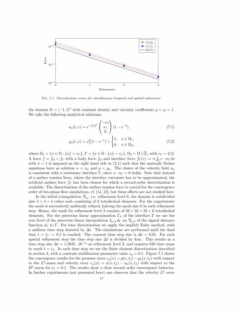
0 1 2 310−4
10−3
10−2
Refinements
Err
or‖ep‖0‖eu‖1O(h2)
Fig. 7.1. Discretization errors for simultaneous temporal and spatial refinement.
the domain Ω = [−1, 1]3 with constant density and viscosity coefficients ρ = µ = 1.We take the following analytical solutions:
ua(t, x) = e−‖x‖2
−x2
x1
0
(1− e−t), (7.1)
pa(t, x) = x31(1− e−t) +
1, x ∈ Ω1,
0, x ∈ Ω2,(7.2)
where Ω1 = x ∈ Ω : ‖x‖ < rΓ, Γ = x ∈ Ω : ‖x‖ = rΓ, Ω2 = Ω \Ω1 with rΓ = 2/3.
A force f = fΩ + fΓ with a body force fΩ and interface force fΓ(v) := σ∫
Γv · nΓ ds
with σ = 1 is imposed on the right hand side in (2.1) such that the unsteady Stokesequations have as solution u = ua and p = pa. The choice of the velocity field uais consistent with a stationary interface Γ, since u · nΓ = 0 holds. Note that insteadof a surface tension force, where the interface curvature has to be approximated, theartificial surface force fΓ has been chosen for which a second-order discretization isavailable. The discretization of the surface tension force is crucial for the convergenceorder of two-phase flow simulations, cf. [14, 12], but these effects are not studied here.
In the initial triangulation Th0 , i.e. refinement level 0, the domain is subdividedinto 4 × 4 × 4 cubes each consisting of 6 tetrahedral elements. For the experimentsthe mesh is successively uniformly refined, halving the mesh size h in each refinementstep. Hence, the mesh for refinement level 3 consists of 32× 32× 32× 6 tetrahedralelements. For the piecewise linear approximation Γh of the interface Γ we use thezero level of the piecewise linear interpolation Ih/2 dΓ on Th/2 of the signed distancefunction dΓ to Γ. For time discretization we apply the implicit Euler method, witha uniform time step denoted by ∆t. The simulations are performed until the finaltime t = tf := 0.1 is reached. The coarsest time step size is ∆t = 0.01. For eachspatial refinement step the time step size ∆t is divided by four. This results in atime step size ∆t = 1.5625 · 10−4 on refinement level 3, and requires 640 time stepsto reach t = tf . In each time step we use the finite element discretization describedin section 2, with a constant stabilization parameter value εp = 0.1. Figure 7.1 showsthe convergence results for the pressure error ep(x) = p(x, tf )− ph(x, tf ) with respectto the L2-norm and velocity error eu(x) = u(x, tf ) − uh(x, tf ) with respect to theH1-norm for tf = 0.1. The results show a clear second order convergence behavior.In further experiments (not presented here) one observes that the velocity L2 error
17
‖eu‖0 also has a second order convergence behavior. This can be explained by thefact that the time discretization error dominates the total error.
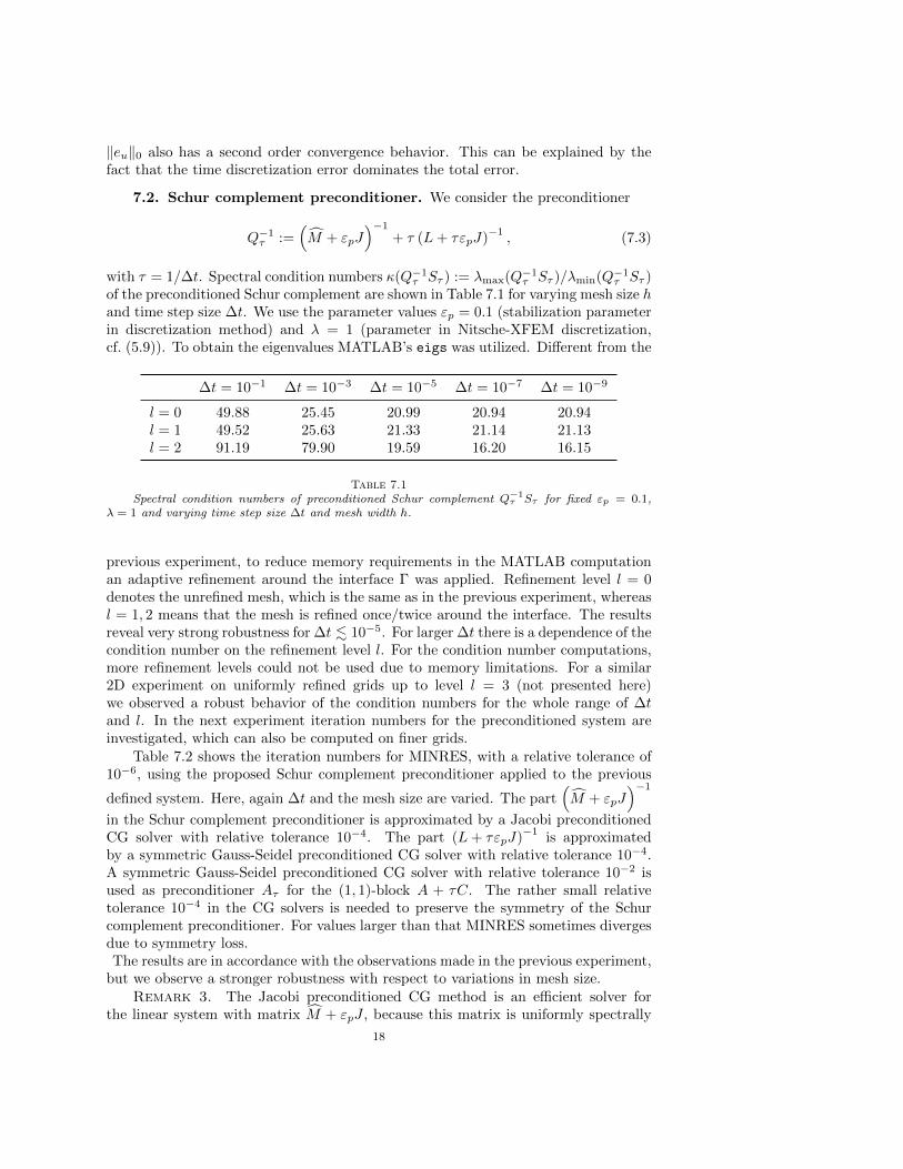
7.2. Schur complement preconditioner. We consider the preconditioner
Q−1τ :=
(M + εpJ
)−1
+ τ (L+ τεpJ)−1, (7.3)
with τ = 1/∆t. Spectral condition numbers κ(Q−1τ Sτ ) := λmax(Q−1
τ Sτ )/λmin(Q−1τ Sτ )
of the preconditioned Schur complement are shown in Table 7.1 for varying mesh size hand time step size ∆t. We use the parameter values εp = 0.1 (stabilization parameterin discretization method) and λ = 1 (parameter in Nitsche-XFEM discretization,cf. (5.9)). To obtain the eigenvalues MATLAB’s eigs was utilized. Different from the
∆t = 10−1 ∆t = 10−3 ∆t = 10−5 ∆t = 10−7 ∆t = 10−9
l = 0 49.88 25.45 20.99 20.94 20.94l = 1 49.52 25.63 21.33 21.14 21.13l = 2 91.19 79.90 19.59 16.20 16.15
Table 7.1Spectral condition numbers of preconditioned Schur complement Q−1
τ Sτ for fixed εp = 0.1,λ = 1 and varying time step size ∆t and mesh width h.
previous experiment, to reduce memory requirements in the MATLAB computationan adaptive refinement around the interface Γ was applied. Refinement level l = 0denotes the unrefined mesh, which is the same as in the previous experiment, whereasl = 1, 2 means that the mesh is refined once/twice around the interface. The resultsreveal very strong robustness for ∆t . 10−5. For larger ∆t there is a dependence of thecondition number on the refinement level l. For the condition number computations,more refinement levels could not be used due to memory limitations. For a similar2D experiment on uniformly refined grids up to level l = 3 (not presented here)we observed a robust behavior of the condition numbers for the whole range of ∆tand l. In the next experiment iteration numbers for the preconditioned system areinvestigated, which can also be computed on finer grids.
Table 7.2 shows the iteration numbers for MINRES, with a relative tolerance of10−6, using the proposed Schur complement preconditioner applied to the previous
defined system. Here, again ∆t and the mesh size are varied. The part(M + εpJ
)−1
in the Schur complement preconditioner is approximated by a Jacobi preconditionedCG solver with relative tolerance 10−4. The part (L+ τεpJ)
−1is approximated
by a symmetric Gauss-Seidel preconditioned CG solver with relative tolerance 10−4.A symmetric Gauss-Seidel preconditioned CG solver with relative tolerance 10−2 isused as preconditioner Aτ for the (1, 1)-block A + τC. The rather small relativetolerance 10−4 in the CG solvers is needed to preserve the symmetry of the Schurcomplement preconditioner. For values larger than that MINRES sometimes divergesdue to symmetry loss.The results are in accordance with the observations made in the previous experiment,
but we observe a stronger robustness with respect to variations in mesh size.Remark 3. The Jacobi preconditioned CG method is an efficient solver for
the linear system with matrix M + εpJ , because this matrix is uniformly spectrally
18
∆t = 10−1 ∆t = 10−3 ∆t = 10−5 ∆t = 10−7 ∆t = 10−9
l = 0 64 46 41 41 42l = 1 64 53 50 53 53l = 2 63 52 47 47 49l = 3 64 49 45 44 45
Table 7.2Iteration numbers of MINRES with constant εp = 0.1, λ = 1 and varying step size ∆t and
mesh width h.
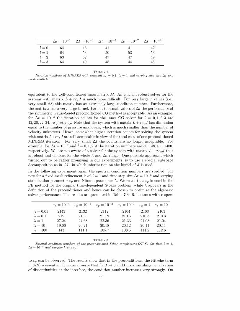
equivalent to the well-conditioned mass matrix M . An efficient robust solver for thesystems with matrix L + τεpJ is much more difficult. For very large τ values (i.e.,very small ∆t) this matrix has an extremely large condition number. Furthermore,the matrix J has a very large kernel. For not too small values of ∆t the performance ofthe symmetric Gauss-Seidel preconditioned CG method is acceptable. As an example,for ∆t = 10−3 the iteration counts for the inner CG solver for l = 0, 1, 2, 3 are42, 26, 22, 24, respectively. Note that the system with matrix L+ τεpJ has dimensionequal to the number of pressure unknowns, which is much smaller than the number ofvelocity unknowns. Hence, somewhat higher iteration counts for solving the systemwith matrix L+τεpJ are still acceptable in view of the total costs of one preconditionedMINRES iteration. For very small ∆t the counts are no longer acceptable. Forexample, for ∆t = 10−9 and l = 0, 1, 2, 3 the iteration numbers are 58, 148, 455, 1480,respectively. We are not aware of a solver for the system with matrix L+ τεpJ thatis robust and efficient for the whole h and ∆t range. One possible approach, whichturned out to be rather promising in our experiments, is to use a special subspacedecomposition as in [27], in which information on the kernel of J is used.
In the following experiment again the spectral condition numbers are studied, butnow for a fixed mesh refinement level l = 1 and time step size ∆t = 10−5 and varyingstabilization parameter εp and Nitsche parameter λ. We recall that εp is used in theFE method for the original time-dependent Stokes problem, while λ appears in thedefinition of the preconditioner and hence can be chosen to optimize the algebraicsolver performance. The results are presented in Table 7.3. Robustness with respect
εp = 10−4 εp = 10−3 εp = 10−2 εp = 10−1 εp = 1 εp = 10
λ = 0.01 2143 2132 2112 2104 2103 2103λ = 0.1 219 215.5 211.9 210.5 210.3 210.3λ = 1 27.24 24.68 22.36 21.33 21.08 21.04λ = 10 19.06 20.21 20.18 20.12 20.11 20.11λ = 100 143 111.1 105.7 108.5 111.2 112.6
Table 7.3Spectral condition numbers of the preconditioned Schur complement Q−1
τ Sτ for fixed l = 1,∆t = 10−5 and varying λ and εp.
to εp can be observed. The results show that in the preconditioner the Nitsche termin (5.9) is essential. One can observe that for λ→ 0 and thus a vanishing penalizationof discontinuities at the interface, the condition number increases very strongly. On
19
the other hand, for λ & 10 one can observe the effect of over-penalization, i.e. a toostrong weight is laid on the continuity across the interface.
Overall, the preconditioner shows robustness for the case of constant coefficientsρ1,2 = µ1,2 ' 1. The robustness holds for a certain range of Nitsche parameter valuesλ ∈ [1, 10].
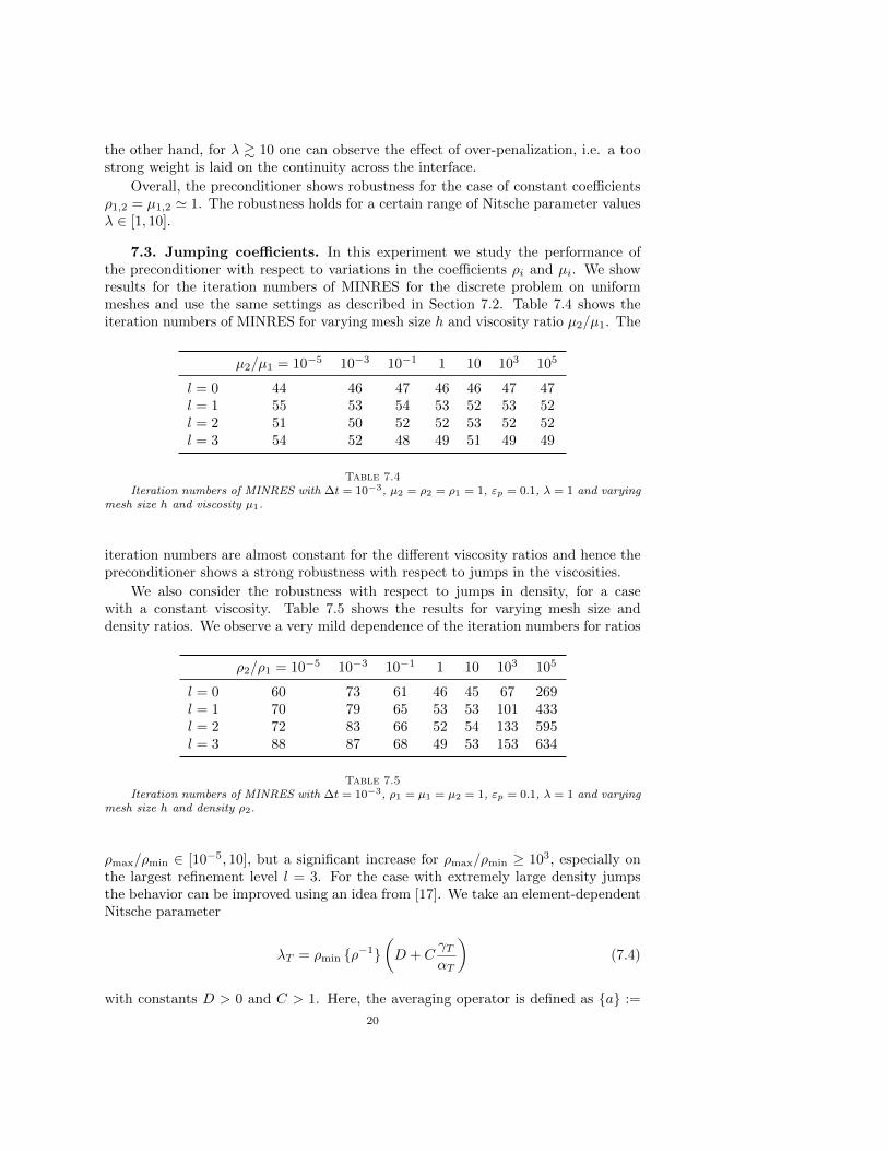
7.3. Jumping coefficients. In this experiment we study the performance ofthe preconditioner with respect to variations in the coefficients ρi and µi. We showresults for the iteration numbers of MINRES for the discrete problem on uniformmeshes and use the same settings as described in Section 7.2. Table 7.4 shows theiteration numbers of MINRES for varying mesh size h and viscosity ratio µ2/µ1. The
µ2/µ1 = 10−5 10−3 10−1 1 10 103 105
l = 0 44 46 47 46 46 47 47l = 1 55 53 54 53 52 53 52l = 2 51 50 52 52 53 52 52l = 3 54 52 48 49 51 49 49
Table 7.4Iteration numbers of MINRES with ∆t = 10−3, µ2 = ρ2 = ρ1 = 1, εp = 0.1, λ = 1 and varying
mesh size h and viscosity µ1.
iteration numbers are almost constant for the different viscosity ratios and hence thepreconditioner shows a strong robustness with respect to jumps in the viscosities.
We also consider the robustness with respect to jumps in density, for a casewith a constant viscosity. Table 7.5 shows the results for varying mesh size anddensity ratios. We observe a very mild dependence of the iteration numbers for ratios
ρ2/ρ1 = 10−5 10−3 10−1 1 10 103 105
l = 0 60 73 61 46 45 67 269l = 1 70 79 65 53 53 101 433l = 2 72 83 66 52 54 133 595l = 3 88 87 68 49 53 153 634
Table 7.5Iteration numbers of MINRES with ∆t = 10−3, ρ1 = µ1 = µ2 = 1, εp = 0.1, λ = 1 and varying
mesh size h and density ρ2.
ρmax/ρmin ∈ [10−5, 10], but a significant increase for ρmax/ρmin ≥ 103, especially onthe largest refinement level l = 3. For the case with extremely large density jumpsthe behavior can be improved using an idea from [17]. We take an element-dependentNitsche parameter
λT = ρmin ρ−1(D + C
γTαT
)(7.4)
with constants D > 0 and C > 1. Here, the averaging operator is defined as a :=
20
κ1a1 + κ2a2 with the element-dependent weights
κ1|T =ρ−1
2 α1,T
ρ−11 α2,T + ρ−1
2 α1,T
, κ2|T =ρ−1
1 α2,T
ρ−11 α2,T + ρ−1
2 α1,T
,
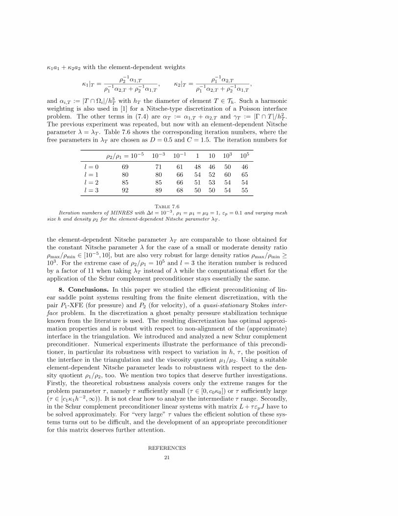
and αi,T := |T ∩ Ωi|/h3T with hT the diameter of element T ∈ Th. Such a harmonic
weighting is also used in [1] for a Nitsche-type discretization of a Poisson interfaceproblem. The other terms in (7.4) are αT := α1,T + α2,T and γT := |Γ ∩ T |/h2
T .The previous experiment was repeated, but now with an element-dependent Nitscheparameter λ = λT . Table 7.6 shows the corresponding iteration numbers, where thefree parameters in λT are chosen as D = 0.5 and C = 1.5. The iteration numbers for
ρ2/ρ1 = 10−5 10−3 10−1 1 10 103 105
l = 0 69 71 61 48 46 50 46l = 1 80 80 66 54 52 60 65l = 2 85 85 66 51 53 54 54l = 3 92 89 68 50 50 54 55
Table 7.6Iteration numbers of MINRES with ∆t = 10−3, ρ1 = µ1 = µ2 = 1, εp = 0.1 and varying mesh
size h and density ρ2 for the element-dependent Nitsche parameter λT .
the element-dependent Nitsche parameter λT are comparable to those obtained forthe constant Nitsche parameter λ for the case of a small or moderate density ratioρmax/ρmin ∈ [10−5, 10], but are also very robust for large density ratios ρmax/ρmin ≥103. For the extreme case of ρ2/ρ1 = 105 and l = 3 the iteration number is reducedby a factor of 11 when taking λT instead of λ while the computational effort for theapplication of the Schur complement preconditioner stays essentially the same.
8. Conclusions. In this paper we studied the efficient preconditioning of lin-ear saddle point systems resulting from the finite element discretization, with thepair P1-XFE (for pressure) and P2 (for velocity), of a quasi-stationary Stokes inter-face problem. In the discretization a ghost penalty pressure stabilization techniqueknown from the literature is used. The resulting discretization has optimal approxi-mation properties and is robust with respect to non-alignment of the (approximate)interface in the triangulation. We introduced and analyzed a new Schur complementpreconditioner. Numerical experiments illustrate the performance of this precondi-tioner, in particular its robustness with respect to variation in h, τ , the position ofthe interface in the triangulation and the viscosity quotient µ1/µ2. Using a suitableelement-dependent Nitsche parameter leads to robustness with respect to the den-sity quotient ρ1/ρ2, too. We mention two topics that deserve further investigations.Firstly, the theoretical robustness analysis covers only the extreme ranges for theproblem parameter τ , namely τ sufficiently small (τ ∈ [0, c0κ0]) or τ sufficiently large(τ ∈ [c1κ1h
−2,∞)). It is not clear how to analyze the intermediate τ range. Secondly,in the Schur complement preconditioner linear systems with matrix L+ τεpJ have tobe solved approximately. For “very large” τ values the efficient solution of these sys-tems turns out to be difficult, and the development of an appropriate preconditionerfor this matrix deserves further attention.
REFERENCES
21
[1] N. Barrau, R. Becker, E. Dubach, and R. Luce, A robust variant of NXFEM for theinterface problem, Comptes Rendus Mathematique, 350 (2012), pp. 789–792.
[2] M. Benzi, G. H. Golub, and J. Liesen, Numerical solution of saddle point problems, Actanumerica, 14 (2005), pp. 1–137.
[3] M. Bercovier and O. Pironneau, Error estimates for finite element method solution of theStokes problem in the primitive variables, Numerische Mathematik, 33 (1979), pp. 211–224.
[4] E. Burman, La penalisation fantome, Comptes Rendus Mathematique, 348 (2010), pp. 1217–1220.
[5] E. Burman, S. Claus, P. Hansbo, M. Larson, and A. Massing, CutFEM: discretizinggeometry and partial differential equations, Intern. J. Numer. Meth. Engng., 104 (2015),pp. 472–501.
[6] E. Burman and P. Hansbo, Fictitious domain finite element methods using cut elements: II.A stabilized Nitsche method, Appl. Numer. Math., 62 (2012), pp. 328–341.
[7] L. Cattanneao, L. Formaggio, G. Iori, A. Scotti, and P. Zunino, Stabilized extended finiteelements for the approximation of saddle point problems with unfitted interfaces, Calcolo,(2014), pp. http://dx.doi.org/10.1007/s10092–014–0109–9.
[8] Y. C. Chang, T. Y. Hou, B. Merriman, and S. Osher, A level set formulation of Eulerianinterface capturing methods for incompressible fluid flows, J. Comp. Phys., 124 (1996),pp. 449–464.
[9] A. Demlow and M. A. Olshanskii, An adaptive surface finite element method based on volumemeshes, SIAM Journal on Numerical Analysis, 50 (2012), pp. 1624–1647.
[10] T. Fries and T. Belytschko, The generalized/extended finite element method: An overviewof the method and its applications, Int. J. Num. Meth. Eng., 84 (2010), pp. 253–304.
[11] V. Girault and P. A. Raviart, Finite Element Methods for Navier-Stokes Equations,Springer, Berlin, 1986.
[12] J. Grande, Finite element discretization error analysis of a general interfacial stress func-tional, Preprint 380, IGPM, RWTH Aachen, 2013. To appear in SIAM J. Numer. Anal.
[13] S. Groß and A. Reusken, An extended pressure finite element space for two-phase incom-pressible flows with surface tension, J. Comp. Phys., 224 (2007), pp. 40–58.
[14] , Finite element discretization error analysis of a surface tension force in two-phaseincompressible flows, SIAM J. Numer. Anal., 45 (2007), pp. 1679–1700.
[15] , Numerical Methods for Two-phase Incompressible Flows, Springer, Berlin, 2011.[16] A. Hansbo and P. Hansbo, An unfitted finite element method, based on Nitsche’s method, for
elliptic interface problems, Comput. Methods Appl. Mech. Engrg., 191 (2002), pp. 5537–5552.
[17] P. Hansbo, M. Larson, and S. Zahedi, A cut finite element method for a Stokes interfaceproblem, Applied Numerical Mathematics, 85 (2014), pp. 90–114.
[18] M. Kirchhart, S. Gross, and A. Reusken, Analysis of an XFEM discretization for Stokesinterface problems, Preprint 420, IGPM, RWTH-Aachen University, 2015. Submitted.
[19] G. M. Kobelkov and M. A. Olshanskii, Effective preconditioning of Uzawa type schemes fora generalized Stokes problem, Numerische Mathematik, 86 (2000), pp. 443–470.
[20] C. Lehrenfeld and A. Reusken, Optimal preconditioners for Nitsche-XFEM discretizationsof interface problems, Preprint 406, IGPM, RWTH Aachen University, 2014. Submitted.
[21] K.-A. Mardal, J. Schoberl, and R. Winther, A uniformly stable Fortin operator for theTaylor-Hood element, Numerische Mathematik, 123 (2013), pp. 537–551.
[22] A. Massing, M. Larson, A. Logg, and M. Rognes, A stabilized Nitsche fictitious domainmethod for the Stokes problem, SIAM J. Sci. Comput., 61 (2014), pp. 604–628.
[23] M. A. Olshanskii, J. Peters, and A. Reusken, Uniform preconditioners for a parameterdependent saddle point problem with application to generalized Stokes interface equations,Numer. Math., 105 (2006), pp. 159–191.
[24] S. Osher and R. P. Fedkiw, Level set methods: An overview and some recent results, J.Comp. Phys., 169 (2001), pp. 463–502.
[25] H. Sauerland and T. Fries, The extended finite element method for two-phase and free-surface flows: A systematic study, J. Comp. Phys., 230 (2011), pp. 3369–3390.
[26] , The stable XFEM for two-phase flows, Computers & Fluids, 87 (2013), pp. 41–49.[27] J. Schoberl, Robust multigrid preconditioning for parameter-dependent problems I: The
Stokes-type case, in Multigrid Methods V, Springer, 1998, pp. 260–275.[28] A.-K. Tornberg and B. Engquist, A finite element based level-set method for multiphase
flow applications, Comput. Visual. Sci., 3 (2000), pp. 93–101.
22