The Surface Energy Balance System (SEBS) for … · The Surface Energy Balance System (SEBS) for...

The Surface Energy Balance System (SEBS) for estimation of turbulent heat fluxes

85

Hydrology and Earth System Sciences, 6(1), 85–99 (2002) © EGS

The Surface Energy Balance System (SEBS) for estimation ofturbulent heat fluxes

Z. SuWageningen University & Research Centre Alterra Green World Research, Wageningen, The Netherlands

Email: [email protected]

AbstractA Surface Energy Balance System (SEBS) is proposed for the estimation of atmospheric turbulent fluxes and evaporative fraction usingsatellite earth observation data, in combination with meteorological information at proper scales. SEBS consists of: a set of tools for thedetermination of the land surface physical parameters, such as albedo, emissivity, temperature, vegetation coverage etc., from spectral reflectanceand radiance measurements; a model for the determination of the roughness length for heat transfer; and a new formulation for the determinationof the evaporative fraction on the basis of energy balance at limiting cases. Four experimental data sets are used to assess the reliabilities ofSEBS. Based on these case studies, SEBS has proven to be capable to estimate turbulent heat fluxes and evaporative fraction at various scaleswith acceptable accuracy. The uncertainties in the estimated heat fluxes are comparable to in-situ measurement uncertainties.

Keywords: Surface energy balance, turbulent heat flux, evaporation, remote sensing

IntroductionThe estimation of atmospheric turbulent fluxes (orevapotranspiration when latent heat flux is expressed inwater depth) at the land surface has long been recognisedas the most important process in the determination of theexchanges of energy and mass among hydrosphere,atmosphere and biosphere (e.g. Bowen, 1926; Penman,1948; Monteith, 1965; Priestly and Taylor, 1972; Brutsaert,1982; Morton, 1983; Famiglietti and Wood, 1994; Sellerset al., 1996; Su and Menenti, 1999; Su and Jacobs, 2001).Conventional techniques that employ point measurementsto estimate the components of energy balance arerepresentative only of local scales and cannot be extendedto large areas because of the heterogeneity of land surfacesand the dynamic nature of heat transfer processes. Remotesensing is probably the only technique which can providerepresentative measurements of several relevant physicalparameters at scales from a point to a continent. Techniquesusing remote sensing information to estimate atmosphericturbulent fluxes are therefore essential when dealing withprocesses that cannot be represented by point measurementsonly.

Methods using remote sensing information to estimateheat exchange between land surface and atmosphere can be

broadly put into two categories: to calculate the sensibleheat flux first and then to obtain the latent heat flux as theresidual of the energy balance equation; or to estimate therelative evaporation by means of an index (e.g. the CropWater Stress Index) using a combination equation (see forexample Menenti, 1984; Bastiaanssen, 1995; Kustas andNorman, 1996; Su and Menenti, 1999 for detailed reviews).Although successful estimations of heat fluxes have beenobtained over small-scale horizontal homogeneous surfaces(Jackson et al., 1981, 1988; Choudhury et al., 1986),difficulties remain in estimations for partial canopies whichare geometrically and thermally heterogeneous (Kalma andJupp, 1990; Zhan et al., 1996). Classical remote sensingflux algorithms based on surface temperature measurementsin combination with spatially constant surfacemeteorological parameters may be suitable for assessing thesurface fluxes on a small scale, but they will fail for largerscales at which the surface meteorological parameters areno longer constant, and the surface geometrical and thermalconditions are neither homogenous nor constant. Hence,more advanced algorithms need to be designed forcomposite terrain at a larger scale with heterogeneoussurfaces.

In this contribution, the Surface Energy Balance System

Z. Su

86

(SEBS) derived by Su (2001) for the estimation ofatmospheric turbulent fluxes using satellite earth observationdata is formulated more coherently and its details areevaluated for the first time. SEBS as proposed here consistsof: a set of tools for the determination of the land surfacephysical parameters, such as albedo, emissivity,temperature, vegetation coverage etc. from spectralreflectance and radiance (Su et al., 1999); an extendedmodel for the determination of the roughness length for heattransfer of Su et al. (2001); and a new formulation for thedetermination of the evaporative fraction on the basis ofenergy balance at limiting cases. In the present set-up, SEBSrequires as inputs three sets of information. The first setconsists of land surface albedo, emissivity, temperature,fractional vegetation coverage and leaf area index, and theheight of the vegetation (or roughness height). Whenvegetation information is not explicitly available, theNormalized Difference Vegetation Index (NDVI) is usedas a surrogate. These inputs can be derived from remotesensing data in conjunction with other information aboutthe concerned surface. The second set includes air pressure,temperature, humidity, and wind speed at a reference height.The reference height is the measurement height for pointapplication and the height of the planetary boundary layer(PBL) for regional application. This data set can also bevariables estimated by a large scale meteorological model.The third data set includes downward solar radiation, anddownward longwave radiation which can either be measureddirectly, model output or parameterisation. Remote sensingmethods used for determination of land surface physicalparameters can be found elsewhere (e.g. Su et al., 1999, Suet al., 1998; Su and Menenti,1999; Li et al., 2000), theemphasis of the present study is on the formulation of SEBSand its validation with four different data sets.

SEBS - The Surface Energy BalanceSystemSURFACE ENERGY BALANCE TERMS

The surface energy balance is commonly written as

EHGRn λ++= 0(1)

where Rn is the net radiation, G0 is the soil heat flux, H isthe turbulent sensible heat flux, and λE is the turbulentlatent heat flux (λ is the latent heat of vapourization and Eis the actual evapotranspiration).

The equation to calculate the net radiation is given by

( ) 401 TRRR lwdswdn ⋅⋅−⋅+⋅−= σεεα (2)

where α is the albedo, Rswd is the downward solar radiation,Rlwd is the downward longwave radiation, ε is the emissivityof the surface, σ is the Stefan-Bolzmann constant, and T0 isthe surface temperature.

The equation to calculate soil heat flux is parameterizedas

( ) ( )[ ]csccn fRG Γ−Γ⋅−+Γ⋅= 10(3)

in which it is assumed that the ratio of soil heat flux to netradiation Γc = 0.05 for full vegetation canopy (Monteith,1973) and Γs = 0.315 for bare soil (Kustas and Daughtry,1989). An interpolation is then performed between theselimiting cases using the fractional canopy coverage, fc.

In order to derive the sensible and latent heat flux, usewill be made of the similarity theory. In this study, distinctionwill be made between the Atmospheric Boundary Layer(ABL) or Planetary Boundary Layer (PBL) and theAtmospheric Surface Layer (ASL). ABL refers to the partof atmosphere that is directly influenced by the presence ofthe Earth’s surface and responds to the surface forcings witha timescale of an hour or less, while ASL refers to usuallythe bottom 10% of ABL (where turbulent fluxes and stressvary by less than 10% of their magnitude, Stull, 1988) butabove the roughness sublayer. The latter (or the interfaciallayer) is the near surface thin layer of a few centimetreswhere molecular transport dominates over turbulenttransport. The thickness of the roughness sublayer is thoughtto be around 35 times the surface roughness height, or threetimes that of the vegetation height (Katul and Parlange,1992). In ASL, the similarity relationships for the profilesof the mean wind speed, u, and the mean temperature,θ0 – θa , are usually written in integral form as

Ψ+

−Ψ−

−=L

zL

dzz

dzkuu m

mmm

00

0

0* ln (4)

Ψ+

−Ψ−

−=−L

zL

dzz

dzCku

H hhh

hpa

00

0

0

*0 ln

ρθθ (5)

where z is the height above the surface, u∗ = (τ0 / ρ)1/2 isthe friction velocity, τ0 is the surface shear stress, ρ is thedensity of air, k = 0.4 is von Karman’s constant, d0 is thezero plane displacement height, z0m is the roughness heightfor momentum transfer, θ0 is the potential temperature atthe surface, θa is the potential air temperature at height z,z0h is the scalar roughness height for heat transfer, ψm andψh are the stability correction functions for momentum andsensible heat transfer respectively, L is the Obukhov lengthdefined as


87

kgHuC

L vp θρ 3*−= (6)

where g is the acceleration due to gravity and θv is thepotential virtual temperature near the surface.

For field measurements performed at a height of a fewmetres above ground, clearly since the surface fluxes arerelated to surface variables and variables in the atmosphericsurface layer, all calculations use the Monin-ObukhovSimilarity (MOS) functions given by Brutsaert (1999). Byreplacing the MOS stability functions with the BulkAtmospheric Boundary Layer (ABL) Similarity (BAS)functions proposed by Brutsaert (1999), the system of Eqns.(4–6) relates surface fluxes to surface variables and themixed layer atmospheric variables. The criterion proposedby Brutsaert (1999) is used to determine if MOS or BASscaling is appropriate for a given situation. The abovefunctions are valid for unstable conditions only. For stableconditions the expressions proposed by Beljaars andHoltslag (1991) and evaluated by van den Hurk and Holtslag(1995) are used for atmospheric surface layer scaling andthe functions proposed by Brutsaert (1982, p.84) foratmospheric boundary layer scaling.

The friction velocity, the sensible heat flux and theObukhov stability length are obtained by solving the systemof non-linear Eqns. (4–6) using the method of Broyden(Press et al., 1997). Derivation of the sensible heat flux usingEqns. (4–6) requires only the wind speed and temperatureat the reference height as well as the surface temperatureand is independent of other surface energy balance terms.

AN EXTENDED MODEL FOR DETERMINATION OFTHE ROUGHNESS LENGTH FOR HEAT TRANSFER

In the above derivations, the aerodynamic and thermaldynamic roughness parameters need to be known. Whennear surface wind speed and vegetation parameters (heightand leaf area index) are available, the within-canopyturbulence model proposed by Massman (1997) can be usedto estimate aerodynamic parameters, d0, the displacementheight, and, z0m, the roughness height for momentum. Thismodel has been shown by Su et al. (2001) to produce reliableestimates of the aerodynamic parameters. If only the heightof the vegetation is available, the relationships proposed byBrutsaert (1982) can be used. If a detailed land useclassification is available, the tabulated values of Wieringa(1986; 1993) can be used. However, since the aerodynamicparameters depend also on wind speed and wind directionas well as the surface characteristics (e.g. Bosveld, 1999),the latter two approaches should be used only when the firstmethod cannot be used due to lack of data. When all of theabove information is not available or not convenient to use,

the aerodynamic parameters can be related to vegetationindices derived from satellite data. However, in this casecare must be taken because the vegetation indices saturateat higher vegetation densities and the relationships aredependent on vegetation type.

The scalar roughness height for heat transfer, z0h, whichchanges with surface characteristics, atmospheric flow andthermal dynamic state of the surface, can be derived fromthe roughness model for heat transfer proposed by Su et al.(2001). However, their model requires a functional form todescribe the vertical structure of the vegetation canopy tocalculate the within-canopy wind speed profile extinctioncoefficient, nec. For local studies, this information is easilyobtained, but for large scale applications, it is generallyimpossible to obtain detailed information on the verticalstructure of the canopy. In this study, nec, is formulated as afunction of the cumulative leaf drag area at the canopy top,

( )22*2 huu

LAICn dec

⋅= (7)

where Cd is the drag coefficient of the foliage elementsassumed to take the value of 0.2, LAI is the one-sided leafarea index defined for the total area, u(h) is the horizontalwind speed at the canopy top. The scalar roughness heightfor heat transfer, z0h, can be derived from

( )100 exp/ −= kBzz mh

(8)

where B–1 is the inverse Stanton number, a dimensionlessheat transfer coefficient. To estimate the kB–1 value, anextended model of Su et al. (2001) is proposed as follows

(9)

where fc is the fractional canopy coverage and fs is itscomplement. Ct is the heat transfer coefficient of the leaf.For most canopies and environmental conditions, Ct isbounded as 0.005N ≤ Ct ≤ 0.075N (N is number of sides ofa leaf to participate in heat exchange) , The heat transfercoefficient of the soil is given by Ct

* = Pr–2/3 Re* –1/2, where

Pr is the Prandtl number and the roughness Reynolds numberRe* = hsu* / v, with hs the roughness height of the soil. Thekinematic viscosity of the air is v = 1.327•10–5 (p0/p)(T/T0)

1.81

(Massman, 1999b), with p and T the ambient pressure andtemperature and p0 = 101.3 kPa and T0 = 273.15 K.Physically and geometrically, the first term of Eqn. (9)

( )( )2

2*

1

14c

nt

d fe

huuC

kCkBec−

− +−

=

( ) 21*

0*

2 sst

hz

huu

sc fkBC

kff

m−+

⋅⋅

Z. Su

88

follows the full canopy only model of Choudhury andMonteith (1988), the third term is that of Brutsaert (1982)for a bare soil surface, while the second term describes theinteraction between vegetation and a bare soil surface. Aquadratic weighting based on the fractional canopy coverageis used to accommodate any situation between the fullvegetation and bare soil conditions. For bare soil surfacekBs

–1 is calculated according to Brutsaert (1982)

( ) [ ]4.7lnRe46.2 41*

1 −=−skB (10)

A NEW FORMULATION FOR DETERMINATION OFEVAPORATIVE FRACTION ON THE BASIS OFENERGY BALANCE AT LIMITING CASES

To determine the evaporative fraction (to be defined below),use is made of energy balance considerations at limitingcases. Under the dry-limit, the latent heat (or the evaporation)becomes zero due to the limitation of soil moisture and thesensible heat flux is at its maximum value.From Eqn. (1), it follows,

0

0 ,0GRH

orHGRE

ndry

dryndry

−=

≡−−=λ (11)

Under the wet-limit, where the evaporation takes place atpotential rate, λEwet , (i.e. the evaporation is limited only bythe energy available under the given surface and atmosphericconditions), the sensible heat flux takes its minimum value,Hwet, i.e.

wetnwet

wetnwet

EGRHorHGRE

λλ

−−=−−=

0

0 , (12)

The relative evaporation then can be evaluated as

wet

wet

wetr E

EEEE

λλλ

λλ −−==Λ 1 (13)

Substitution of Eqns. (1), (12) and (11) in Eqn. (13) andafter some algebra:

wetdry

wetr HH

HH−

−−=Λ 1 (14)

The actual sensible heat flux H defined by Eqn. (5) isconstrained in the range set by the sensible heat flux at thewet limit Hwet, and the sensible heat flux at the dry limitHdry . Hdry is given by Eqn. (11) and Hwet can be derived by

combining Eqn. (12) and a combination equation similar tothe Penman-Monteith combination equation (Monteith,1965). Menenti (1984) showed that, when the resistanceterms are grouped into the bulk internal (or surface, orstomatal) and external (aerodynamic) resistances, thecombination equation can be written in the following form

( ) ( )( ) ie

satpne

rreeCGRr

E⋅+∆+⋅

−⋅+−⋅⋅∆=

γγρ

λ 0 (15)

where e and esat are actual and saturation vapour pressurerespectively; γ is the psychrometric constant, and ∆ is therate of change of saturation vapour pressure withtemperature (i.e. ( ) TTesat ∂∂ ); ri is the bulk surface internalresistance and re is the external or aerodynamic resistance.In the above equation it is assumed that the roughnesslengths for heat and vapour transfer are the same (Brutsaert,1982). The Penman-Monteith equation is strictly valid onlyfor a vegetated canopy, whereas the definition by Eqn. (15)is also valid for a soil surface with properly defined bulkinternal resistance. The difficulty in using Eqn. (15) toestimate latent heat flux lies in the difficulty to determinethe bulk internal resistance ri which is regulated by soilwater availability. Because the latter is generally not knowna priori, an alternative is thus proposed in this study to avoidthe direct use of ri in estimating λE.

At the wet-limit, the internal resistance 0≡ir bydefinition. Using this property in Eqn. (15) and changingthe subscripts correspondingly to reflect the wet-limitcondition, the sensible heat flux at the wet-limit is obtainedas:

( )

∆+

−⋅−−=γγ

ρ10

eerC

GRH s

ew

pnwet (16)

The external resistance depends also on the Obukhovlength, L, which in turn is a function of the friction velocityand sensible heat flux (Eqns. 4–6). With the friction velocityand the Obukhov length determined by the numericalprocedure described previously, the external resistance canbe determined from Eqn. (5) as:

Ψ+

−Ψ−

−=L

zLdz

zdz

kur h

hhh

e00

0

0

*

ln1 (17)

Similarly, the external resistance at the wet-limit can bederived as

Ψ+

−Ψ−

−=w

hh

wh

hew L

zL

dzz

dzku

r 00

0

0

*

ln1 (18)

The wet-limit stability length can be determined as:

( ) λρ

0

3*

61.0 GRkguL

nw −⋅⋅

−= (19)


89

The evaporative fraction is finally given by:

GRE

GRE

n

wetr

n −⋅Λ=

−=Λ λλ (20)

By inverting Eqn. (20), the actual latent heat flux λE can beobtained.

Eqns. (1–20) constitute the formulation of SEBS; itsvalidation using four different data sets is the subject of thefollowing sections.

Data and materialsThree field datasets obtained from flux stations and oneremote sensing dataset are used in this study. The fielddatasets have been used extensively for validation purposes(e.g. Norman et al., 1995; Zhan et al., 1996; Kustas andNorman, 1999). The remote sensing dataset was collectedduring the EFEDA field experiment (Bolle et al., 1993).

COTTON DATA

This dataset was collected over a cotton field in MaricopaFarms in central Arizona from 10 to 14 June 1987. Thefield is 1500 metres east-west by 300 metres north-south,with cotton rows 0.2 m in width and spaced at 1 m apart,running north-south. The cotton plants are some 0.32 m highon top of a 0.17 m high furrow. Profile measurements ofwind and temperature at five levels were used to derive thezero plane displacement and the roughness height formomentum. Sensible and latent heat fluxes were measuredby the Bowen ratio and eddy correlation method. Themeasurements of the latter (at a height of three metres) areused in this study for validation of the SEBS estimates.Complete descriptions of this dataset are given by Kustaset al. (1989a,b), Kustas and Daughtry (1989) and Kustas(1990), covering instrumentation, the agronomicmeasurements, the derivation of aerodynamic roughnessparameters, the determination of the composite surfaceradiometric temperature, the determination of the soil heatflux and the modelling of the heat fluxes with a one- andtwo-layer model. The composite surface radiometrictemperature is derived by weighting the measuredradiometric temperatures of the shaded soil, sunlit soil, andvegetation with the actual areas covered by these portions(Kustas and Daughtry, 1989).

In this study, the effective height of the surface isdetermined as the cotton plant height, 0.32 m, weighted byits fractional coverage of 0.24. The leaf area index is 0.4. Intotal, 19 data points, all from day-time hours (from 09.23 to

15.02 h), are available with all the required information.

SHRUB DATA

The shrub dataset was collected in the Lucky Hills studyarea, a shrub-dominated ecosystem, during theMONSOON’90 multidisciplinary experiment conductedover the U.S. Department of Agriculture’s AgriculturalResearch Service Walnut Gulch experimental basin in south-eastern Arizona during June–September 1990 (see Kustasand Goodrich, 1994). Data from the second observationperiod from mid-July to early August are used in this study.These include ground-based continuous measurements ofmeteorological conditions at screen heights, near-surfacesoil temperature and soil moisture, surface temperature,incoming solar and net radiation, soil heat flux, and indirectdetermination of sensible and latent heat fluxes (Kustas etal., 1994a,b). Detailed measurements on vegetation type,height and fractional cover and surface soil properties weremade at each site (Weltz et al., 1994). There were large andsmall shrubs present: the height of the large shrubs wasdetermined as 0.5 m, which is weighted by the fractionalcoverage of 0.26 and used in the calculation. The leaf areaindex is 0.4. The reference height for measurements of windspeed is 4.3 m. The study used 320 hourly-average datapoints, from both day-time and night-time hours from day209 to day 220, and with all required variables available.

GRASS DATA

The grass dataset was also collected during theMONSOON’90 multidisciplinary experiment in the Kendallstudy area, a grass-dominated ecosystem. All themeasurements are similar to the shrub data. At the grasssite, the surface was also complex, consisting of shrubs, tallgrass and low grass. The averaged grass height wasestimated as 0.1 m. Similarly, an effective height is used bymultiplying the average grass height with the fractionalcoverage of 0.44. The leaf area index is 0.8 and the referenceheight is again 4.3 metres. This study used 281 hourly-average data points, also from both day-time and night-timehours from day 210 to day 220, and with all requiredvariables available.

EFEDA DATA

The remote sensing data obtained with the Thematic MapperSimulator (TMS-NS001) during the EFEDA campaign(Bolle et al., 1993) for the Barrax region in Spain is used.The TMS data were taken from NASA’s ER2 aircraft forthe Barrax area in Spain on 29 June 1991, 12.21 GMT, with18.5 m ground resolution. In addition, radiosonde and half-

Z. Su

90

hourly surface tower flux, as well as surface radiationmeasurements at the same time as the over-flight are usedto determine regionally constant parameters. These variablesinclude atmospheric transmissivity, potential air temperatureat the blending height and the incoming long-wave radiationat the time of the remote sensing data collection. The spatialresolution of the data, 18.5 m, is considered to be sufficientto characterise the heterogeneity of the surface under study.The estimation of the physical parameters from the TMSdata from the surface (albedo, temperature and vegetationindices) follows Su et al. (1999).

Results and discussionsThe accuracy of SEBS will be assesed by analysis carriedout separately for each of the four datasets. For the fielddatasets, the aerodynamic parameters are the modelestimates as discussed previously. All other input variablesare measured except the downward long-wave radiation thatis estimated with the Stefan-Boltzman radiation equationusing the air temperature measured at the reference height.The emissivity of the air is estimated using the formula ofSwinbank (Campbell and Norman, 1998, p.164) whichrequires only air temperature. The measured albedo valuesare not available so a value is chosen for each dataset thatkeeps the radiation terms in balance. The surface emissivityvalues are measured (Kustas et al., 1989b; Humes et al.,1994).

RESULTS FOR COTTON DATA

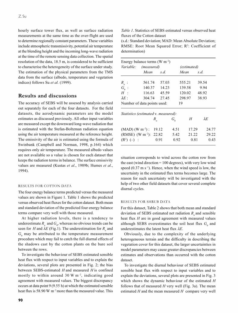
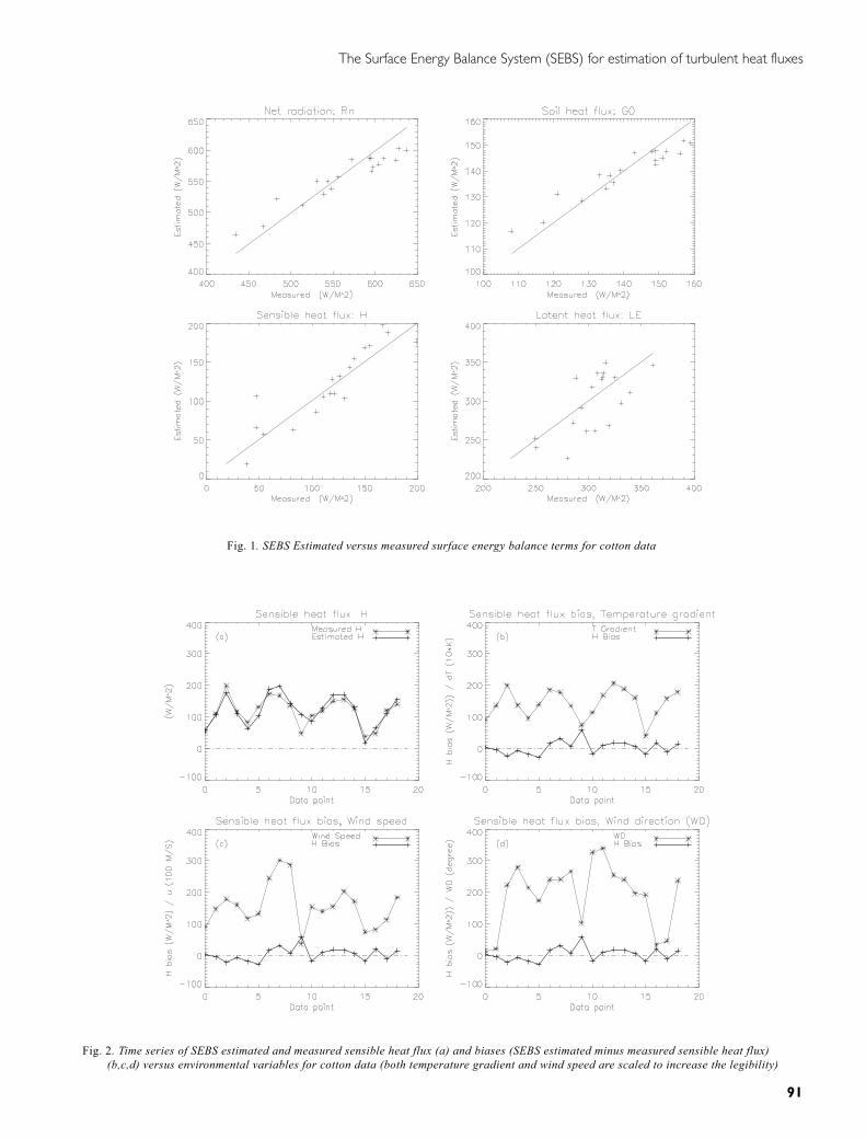
The four energy balance terms predicted versus the measuredvalues are shown in Figure 1. Table 1 shows the predictedversus observed heat fluxes for the cotton dataset. Both meanand standard deviation of the predicted four energy balanceterms compare very well with those measured.

At higher radiation levels, there is a tendency tounderestimate Rn and G0, whereas no obvious trends can beseen for H and λE (Fig.1). The underestimation for Rn andG0 may be attributed to the temperature measurementprocedure which may fail to catch the full diurnal effects ofthe shadows cast by the cotton plants on the bare soilbetween the rows.

To investigate the behaviour of SEBS estimated sensibleheat flux with respect to input variables and to explain thedeviations, several plots are presented in Fig. 2; the biasbetween SEBS-estimated H and measured H is confinedmostly to within around 30 W m–2, indicating goodagreement with measured values. The biggest discrepancyoccurs at data point 9 (9.55 h) at which the estimated sensibleheat flux is 58.90 W m–2 more than the measured value. This

situation corresponds to wind across the cotton row fromthe east (wind direction = 100 degrees), with very low windspeed (0.37 m s–1). Hence, when the wind speed is low, theuncertainty in the estimated flux terms becomes large. Thereason for such uncertainty will be investigated with thehelp of two other field datasets that cover several completediurnal cycles.

RESULTS FOR SHRUB DATA

For this dataset, Table 2 shows that both mean and standarddeviation of SEBS estimated net radiation Rn and sensibleheat flux H are in good agreement with measured valuesalthough SEBS overestimates the soil heat flux G0 andunderestimates the latent heat flux λE.

Obviously, due to the complexity of the underlyingheterogeneous terrain and the difficulty in describing thevegetation cover for this dataset, the larger uncertainties inmodel parameters may cause greater discrepancies betweenestimates and observations than occurred with the cottondataset.

To investigate the diurnal behaviour of SEBS estimatedsensible heat flux with respect to input variables and toexplain the deviations, several plots are presented in Fig. 3which shows the dynamic behaviour of the estimated Hfollows that of measured H very well (Fig. 3a). The meanestimated H and the mean measured H compare very well

Table 1. Statistics of SEBS estimated versus observed heatfluxes of the Cotton dataset(s.d.: Standard deviation; MAD: Mean Absolute Deviation;RMSE: Root Mean Squared Error; R2: Coefficient ofdetermination)

Energy balance terms (W m–2)Variable: (measured) (estimated)

Mean s.d. Mean s.d.

Rn : 561.74 57.03 555.21 39.54G0 : 140.37 14.23 139.58 9.94H : 116.63 45.59 120.02 48.92λE : 304.74 27.45 298.97 38.93Number of data points used: 19

Statistics (estimated v. measured):Rn G0 H λE

(MAD) (W m–2) : 19.12 4.51 17.29 24.77(RMSE) (W m–2): 22.82 5.42 21.22 29.22(R2) (–) : 0.91 0.92 0.81 0.43


91

Fig. 1. SEBS Estimated versus measured surface energy balance terms for cotton data

Fig. 2. Time series of SEBS estimated and measured sensible heat flux (a) and biases (SEBS estimated minus measured sensible heat flux)(b,c,d) versus environmental variables for cotton data (both temperature gradient and wind speed are scaled to increase the legibility)

Z. Su

92

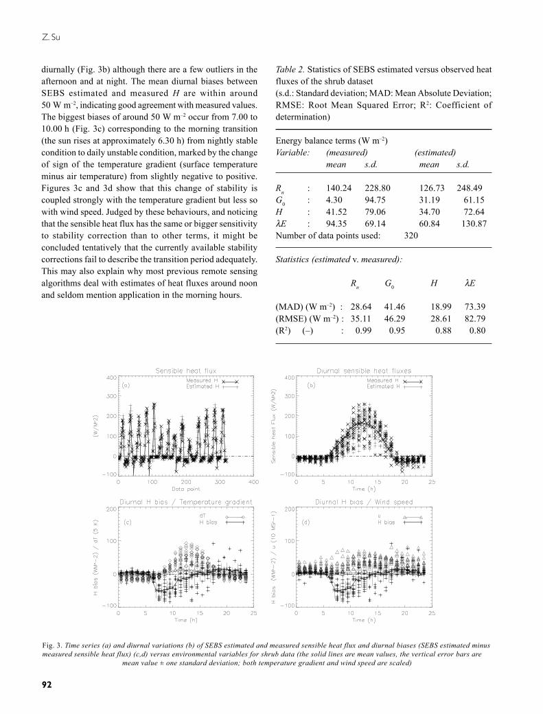
diurnally (Fig. 3b) although there are a few outliers in theafternoon and at night. The mean diurnal biases betweenSEBS estimated and measured H are within around50 W m–2, indicating good agreement with measured values.The biggest biases of around 50 W m–2 occur from 7.00 to10.00 h (Fig. 3c) corresponding to the morning transition(the sun rises at approximately 6.30 h) from nightly stablecondition to daily unstable condition, marked by the changeof sign of the temperature gradient (surface temperatureminus air temperature) from slightly negative to positive.Figures 3c and 3d show that this change of stability iscoupled strongly with the temperature gradient but less sowith wind speed. Judged by these behaviours, and noticingthat the sensible heat flux has the same or bigger sensitivityto stability correction than to other terms, it might beconcluded tentatively that the currently available stabilitycorrections fail to describe the transition period adequately.This may also explain why most previous remote sensingalgorithms deal with estimates of heat fluxes around noonand seldom mention application in the morning hours.

Fig. 3. Time series (a) and diurnal variations (b) of SEBS estimated and measured sensible heat flux and diurnal biases (SEBS estimated minusmeasured sensible heat flux) (c,d) versus environmental variables for shrub data (the solid lines are mean values, the vertical error bars are

mean value ± one standard deviation; both temperature gradient and wind speed are scaled)

Table 2. Statistics of SEBS estimated versus observed heatfluxes of the shrub dataset(s.d.: Standard deviation; MAD: Mean Absolute Deviation;RMSE: Root Mean Squared Error; R2: Coefficient ofdetermination)


mean s.d. mean s.d.


Statistics (estimated v. measured):

Rn G0 H λE

(MAD) (W m–2) : 28.64 41.46 18.99 73.39(RMSE) (W m–2) : 35.11 46.29 28.61 82.79(R2) (–) : 0.99 0.95 0.88 0.80


93

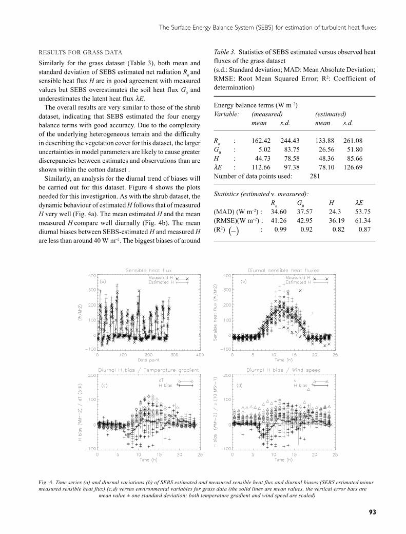
RESULTS FOR GRASS DATA

Similarly for the grass dataset (Table 3), both mean andstandard deviation of SEBS estimated net radiation Rn andsensible heat flux H are in good agreement with measuredvalues but SEBS overestimates the soil heat flux G0 andunderestimates the latent heat flux λE.

The overall results are very similar to those of the shrubdataset, indicating that SEBS estimated the four energybalance terms with good accuracy. Due to the complexityof the underlying heterogeneous terrain and the difficultyin describing the vegetation cover for this dataset, the largeruncertainties in model parameters are likely to cause greaterdiscrepancies between estimates and observations than areshown within the cotton dataset .

Similarly, an analysis for the diurnal trend of biases willbe carried out for this dataset. Figure 4 shows the plotsneeded for this investigation. As with the shrub dataset, thedynamic behaviour of estimated H follows that of measuredH very well (Fig. 4a). The mean estimated H and the meanmeasured H compare well diurnally (Fig. 4b). The meandiurnal biases between SEBS-estimated H and measured Hare less than around 40 W m–2. The biggest biases of around

Table 3. Statistics of SEBS estimated versus observed heatfluxes of the grass dataset(s.d.: Standard deviation; MAD: Mean Absolute Deviation;RMSE: Root Mean Squared Error; R2: Coefficient ofdetermination)


mean s.d. mean s.d.


Statistics (estimated v. measured):Rn G0 H λE

(MAD) (W m–2) : 34.60 37.57 24.3 53.75(RMSE)(W m–2) : 41.26 42.95 36.19 61.34(R2) ( )− : 0.99 0.92 0.82 0.87

Fig. 4. Time series (a) and diurnal variations (b) of SEBS estimated and measured sensible heat flux and diurnal biases (SEBS estimated minusmeasured sensible heat flux) (c,d) versus environmental variables for grass data (the solid lines are mean values, the vertical error bars are

mean value ± one standard deviation; both temperature gradient and wind speed are scaled)

Z. Su

94

40 W m–2 occur from 7.00 to 9.00 h (Fig. 4c) correspondingto the morning transition (the sun rises at approximately6.30 h) from the nightly stable condition to the daily unstablecondition. Figures 4c and 4d show that the change in stabilityin this case is also coupled with the temperature gradientbut less so with wind speed. This confirms that, as for theshrub dataset, the currently available stability correctionsfail to describe the transition period. However, in contrastto the shrub data, bigger biases are also observed at 18.00and 19.00 h. This situation corresponds to the transition fromunstable to stable condition and is also coupled to thetemperature gradient but not so much to the wind.

RESULTS FOR EFEDA DATA

First of all, the primary inputs to SEBS are derived in thesame way as Su et al. (1999) and Su and Jacobs (2001).These inputs include: remote sensing physical variablesderived from the TMS data (albedo, surface temperature,and Normalized Difference Vegetation Index) andradiosonde and surface in-situ data (clear sky downwardshortwave radiation, clear sky downward longwaveradiation, PBL-height, surface pressure, PBL-averagedspecific humidity, PBL-averaged potential temperature,PBL-averaged horizontal wind speed). Other derivedvariables are described in Su and Jacobs (2001). The relevantinputs for this study are given in Table 4.

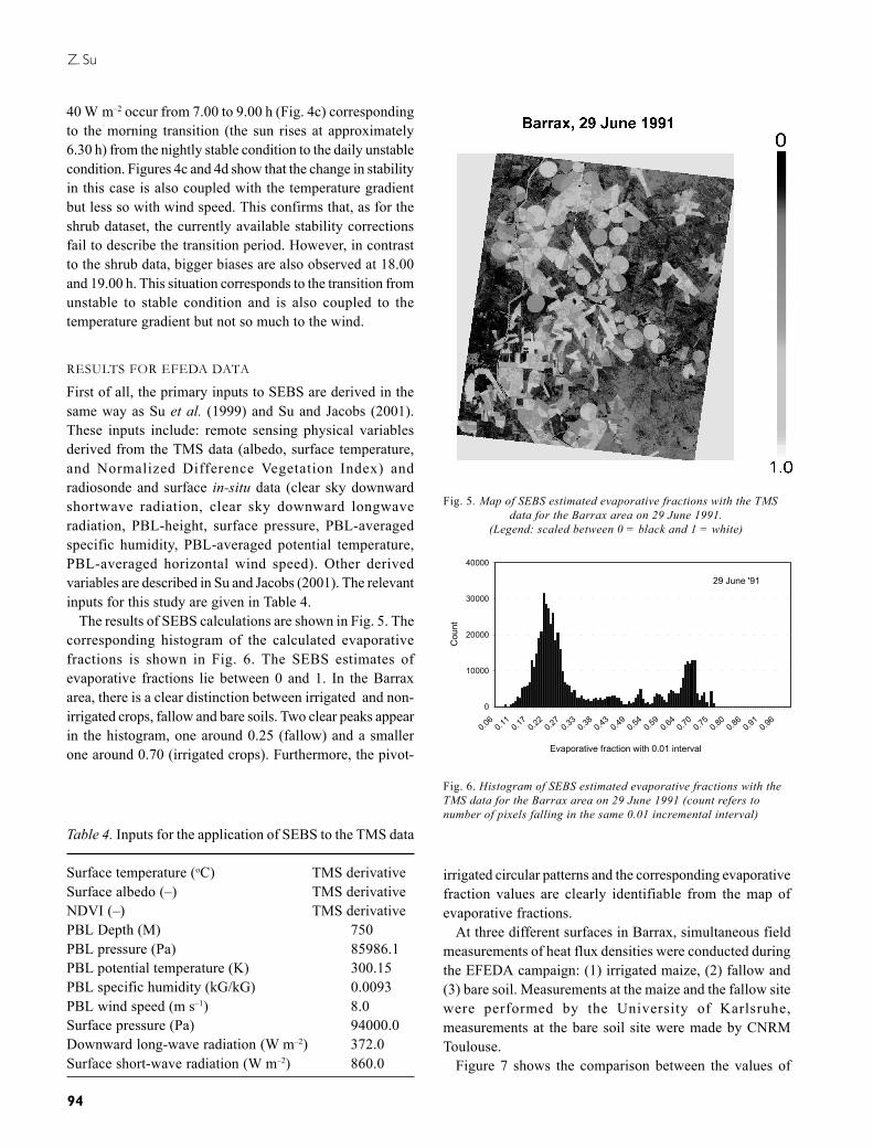
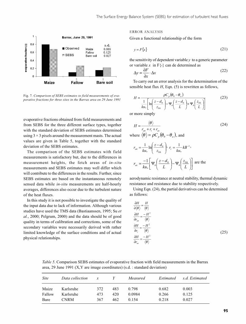
The results of SEBS calculations are shown in Fig. 5. Thecorresponding histogram of the calculated evaporativefractions is shown in Fig. 6. The SEBS estimates ofevaporative fractions lie between 0 and 1. In the Barraxarea, there is a clear distinction between irrigated and non-irrigated crops, fallow and bare soils. Two clear peaks appearin the histogram, one around 0.25 (fallow) and a smallerone around 0.70 (irrigated crops). Furthermore, the pivot-

Table 4. Inputs for the application of SEBS to the TMS data

Surface temperature (oC) TMS derivativeSurface albedo (–) TMS derivativeNDVI (–) TMS derivativePBL Depth (M) 750PBL pressure (Pa) 85986.1PBL potential temperature (K) 300.15PBL specific humidity (kG/kG) 0.0093PBL wind speed (m s–1) 8.0Surface pressure (Pa) 94000.0Downward long-wave radiation (W m–2) 372.0Surface short-wave radiation (W m–2) 860.0

Fig. 5. Map of SEBS estimated evaporative fractions with the TMSdata for the Barrax area on 29 June 1991.

(Legend: scaled between 0 = black and 1 = white)

29 June '91

0

10000

20000

30000

40000

0.06

0.11

0.17

0.22

0.27

0.33

0.38

0.43

0.49

0.54

0.59

0.64

0.70

0.75

0.80

0.86

0.91

0.96

Evaporative fraction with 0.01 interval

Cou

nt

Fig. 6. Histogram of SEBS estimated evaporative fractions with theTMS data for the Barrax area on 29 June 1991 (count refers tonumber of pixels falling in the same 0.01 incremental interval)

irrigated circular patterns and the corresponding evaporativefraction values are clearly identifiable from the map ofevaporative fractions.

At three different surfaces in Barrax, simultaneous fieldmeasurements of heat flux densities were conducted duringthe EFEDA campaign: (1) irrigated maize, (2) fallow and(3) bare soil. Measurements at the maize and the fallow sitewere performed by the University of Karlsruhe,measurements at the bare soil site were made by CNRMToulouse.

Figure 7 shows the comparison between the values of


95

Table 5. Comparison SEBS estimates of evaporative fraction with field measurements in the Barraxarea, 29 June 1991 (X,Y are image coordinates) (s.d. : standard deviation)

Site Data collection x Y Measured Estimated s.d. Estimated

Maize Karlsruhe 372 483 0.798 0.682 0.003Fallow Karlsruhe 473 420 0.0984 0.266 0.125Bare CNRM 367 462 0.154 0.218 0.027

Fig. 7. Comparison of SEBS estimates to field measurements of eva-porative fractions for three sites in the Barrax area on 29 June 1991

evaporative fractions obtained from field measurements andfrom SEBS for the three different surface types, togetherwith the standard deviation of SEBS estimates determinedusing 3 × 3 pixels around the measurement masts. The actualvalues are given in Table 5, together with the standarddeviation of the SEBS estimates.

The comparison of the SEBS estimates with fieldmeasurements is satisfactory but, due to the differences inmeasurement heights, the fetch areas of in-situmeasurements and SEBS estimates may well differ whichwill contribute to the differences in the results. Further, sinceSEBS estimates are based on the instantaneous remotelysensed data while in-situ measurements are half-hourlyaverages, differences also occur due to the turbulent natureof the heat fluxes.

In this study it is not possible to investigate the quality ofthe input data due to lack of information. Although variousstudies have used the TMS data (Bastiaanssen, 1995; Su etal., 2000; Pelgrum, 2000) and the data should be of goodquality in terms of calibration and corrections, some of thesecondary variables were necessarily derived with ratherlimited knowledge of the surface conditions and of actualphysical relationships.

ERROR ANALYSIS

Given a functional relationship of the form

{ }xFy = (21)

the sensitivity of dependent variable y to a generic parameteror variable x in F{•} can de determined as

xxFy ∆⋅

∂∂=∆ (22)

To carry out an error analysis for the determination of thesensible heat flux H, Eqn. (5) is rewritten as follows,

( )

Ψ+

−Ψ−

−

−=

Lz

Ldz

zdz

ku

CH

hhh

h

ap

00

0

0

*

0

ln1

θθρ(23)

or more simply

astan rrrH

++=

θ (24)

where ( )apC θθρθ −= 0 , and

−=h

an zdz

kur

0

0

*

ln1 , 1

*

1 −= kBku

rt,

Ψ−

−Ψ−=

Lz

Ldz

kur h

hhas00

*

1 are the

aerodynamic resistance at neutral stability, thermal dynamicresistance and resistance due to stability respectively.

Using Eqn. (24), the partial derivatives can be determinedas follows:

θ

θ

θ

θθ

2

2

2

HrH

HrH

HrH

HH

as

t

an

−=∂∂

−=∂∂

−=∂∂

=∂∂

(25)

Z. Su

96

Substitution of Eqn. (25) into Eqn. (22), yields the sensi-tivity of H to each term in Eqn. (24.).

Using the range of values from the cotton data, i.e. H = 50~ 200 (W m–2), u* =0.05 ~ 0.3 (MS-1), and (θ0 – θa) =5 ~ 20(K), the sensitivity in Eqn. (24) to each term can also beapplied to the primary terms, (θ0 – θa), u*, kB–1, and Ψh

respectively. These sensitivities are given as:∆H = 10•∆(θ0 – θa), ∆H = 148•∆u*, ∆H = –25•∆kB–1,∆H = –25•∆Ψh. Inserting typical values for the uncertaintiesof the primary terms, the sensitivities are quantified as: 20,11, –25 and –25 (W m–2), for ∆(θ0 – θa) = 2K, ∆u* = 25%,∆kB–1 = 1, ∆Ψh = 1, respectively. When the various termsare assumed independent of each other, the total uncertaintyis around 40 (W m–2). Since in reality, at least some of theterms are correlated, the expected sensitivity can then beestimated in the order of 20 (W m–2), which is around 20%relative to the mean sensible heat flux H.

In a previous study, Su et al. (2001) have investigated thesensitivity of kB–1 to the physical and geometrical variablesused in Eqn. (9) using a simpler version than Eqn. (9). Bychanging variable values as much as 50% with respect toreference values, they showed that the sensitivity of kB–1 toall parameters, except vegetation height, is comparable andthe errors in the computed H are bounded by 37% relativeto the mean measured H. The sensitivity of H to vegetationheight approaches 46% of the mean measured H by far thelargest. Since current SEBS formulation is superior to thatused for the sensitivity analysis in Su et al. (2001) (theRMSE is 21.22 W m–2 in the present study, whereas it was27.29 W m-2), SEBS can give reliable estimates of H, aslong as the variables used are accurate to within 50% oftheir actual values.

General remarksAfter the derivation of sensible heat flux by solving Eqns.(4–6), the latent heat flux can be estimated as a residual bymeans of Eqn. (1), (e.g. Kalma and Jupp, 1990; Su, 2001).However, the uncertainty associated with the derived latentheat flux and consequently with the evaporative fraction islarge, because the sensible heat flux is, under given surfaceconditions, determined solely by the surface temperatureand the meteorological conditions at the reference heightand is not constrained by the available energy. If the surfacetemperature or the meteorological variables have largeuncertainties, the resultant latent heat flux and evaporativefraction will be affected. In the SEBS formulation, thisuncertainty is limited by consideration of the energy balanceat the limiting cases: the actual sensible heat flux H liesbetween the sensible heat flux at the wet limit Hwet derivedfrom the combination equation, and the sensible heat flux

at the dry limit Hdry set by the available energy.In this respect, SEBS is similar to previous algorithms

that estimate relative evaporation by means of an index (e.g.the Crop Water Stress Index) using a combination equation(Jackson et al., 1981, 1988; Menenti and Choudhury, 1993;Moran et al., 1994; Pelgrum, 2000; Menenti et al., 2001).However, none of these algorithms incorporated theformulation of the roughness height for heat transferexplicitly; instead they used fixed values. Since theroughness height for heat transfer can vary with geometricand environmental variables by several orders of magnitudefor different surface types, this can cause great uncertaintiesin estimation of heat fluxes or evaporation using radiometrictemperature measurements (e.g. Verhoef et al., 1997;Massman, 1999a; Blümel, 1999; Su et al., 2001). Althoughit is possible to calibrate these algorithms such that theirestimates reproduce observations at local scale, it would bevery difficult to extrapolate them to regional/continentalstudies by means of satellite observations.

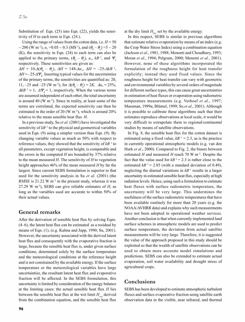
In Fig. 8, the sensible heat flux for the cotton dataset isestimated using a fixed value, kB–1 = 2.3, as is the practicein currently operational atmospheric models (e.g. van denHurk et al., 2000). Compared to Fig. 2, the biases betweenestimated H and measured H reach 70 W m–2. Despite thefact that the value used for kB–1 = 2.3 is rather close to theestimated kB–1 = 2.85 (with a standard deviation of 0.49),neglecting the diurnal variations in kB–1 results in a largeruncertainty in estimated sensible heat flux, especially at highradiation levels. Hence, using such a formulation to estimateheat fluxes with surface radiometric temperature, theuncertainty will be very large. This undermines theusefulness of the surface radiometric temperatures that havebeen available routinely for more than 20 years (e.g. theNOAA/AVHRR data) and explains why such measurementshave not been adopted in operational weather services.Another conclusion is that when currently implemented landsurface schemes in atmospheric models are used to predictsurface temperature, the deviation from actual satellitemeasurements will be very large. Therefore, it is suggestedthe value of the approach proposed in this study should beexploited so that the wealth of satellite observations can beused to obtain more accurate model simulations andpredictions. SEBS can also be extended to estimate actualevaporation, soil water availability and drought stress ofagricultural crops.

ConclusionsSEBS has been developed to estimate atmospheric turbulentfluxes and surface evaporative fraction using satellite earthobservation data in the visible, near infrared, and thermal


97

infrared frequency range, in combination withmeteorological data from a proper reference height givenby either in-situ measurements for application to a point,and radiosonde or meteorological forecasts for applicationat larger scales.

SEBS has been applied to four different data sets derivedfrom radiometric and meteorological measurements. On thebasis of these experimental validations, SEBS can be usedto estimate turbulent heat fluxes at different scales withacceptable accuracy. Some specific conclusions are asfollows:

The mean error of SEBS estimates is expected to bearound 20% relative to the mean sensible heat flux H,when the input geometrical and physical variables arereliable. For regional scale applications, SEBS can givereliable estimates of H, as long as the geometricalvariables used are accurate to within 50% of their actualvalues and the physical variables are accurate to∆(θ0 – θa) = 2K and ∆u* = 25%.

The errors in estimated sensible heat flux H due touncertainty in roughness height for heat transfer givenby Eqns. (8–9), are bigger than or comparable to thosedue to uncertainties in temperatures, wind speed andstability corrections. The extended model of Su et al.(2001) proposed here (Eqn. 9) provides an operationalsolution for regional scale applications using remotelysensed data.Currently available stability corrections are inadequatein describing the transition from nightly stable to dailyunstable conditions.

Finally, the application of SEBS does not require any apriori knowledge of the actual turbulent heat fluxes,indicating that SEBS is a credible and independent approach.Due to this property, SEBS results may be used to validateand initialise hydrological, atmospheric and ecologicalmodels that usually require proper partition of the sensibleand latent heat flux at different scales. SEBS results mayalso be used via data assimilation in the above models to

Fig. 8. Same as Figure 2 for the cotton data, but estimated using a fixed value, 1−kB =2.3, as used in currently operationalatmospheric models

Z. Su

98

increase the reliability of the model simulations andpredictions. Another approach would be to implement therepresentation of surface flux exchanges as described inSEBS into a Land Data Assimilation System (LDAS: see,for example, http://ldas.gsfc.nasa.gov/LDASnew/index.html), then to assimilate the remotely-sensed data,including surface temperature, into the LDAS using moderndata assimilation techniques. As evidenced by thepresentations at the “International Workshop on Catchment-scale Hydrological Modelling and Data Assimilation,Wageningen, Sep. 3-5, 2001 (http://www.wau.nl/whh/wrkshp/), advances in improving parameterisation andpredictability of hydrological models, physically-baseddistributed models in particular, will rely heavily on theunderstanding of physical processes at different scales aswell as the ability to obtain distributed physical information;satellite Earth observation will prove of paramountimportance in the future.

AcknowledgementsThis work was funded jointly by the Dutch Remote SensingBoard (BCRS), the Dutch Ministry of Agriculture, NatureManagement and Fisheries (LNV), and the RoyalNetherlands Academy of Science (KNAW). Constructivecomments and assistance from Li Jia, Gerbert Roerink,Claire Jacobs, Jun Wen, Han Rauwerda (Alterra) and Bartvan den Hurk (KNMI) are gratefully appreciated. The authoris grateful to Bill Kustas (USDA/ARS) who kindly providedthe three field data sets used in this study. The author is alsograteful to the editor and three anonymous reviewers fortheir frank and constructive criticisms.

ReferencesBastiaanssen, W.G.M., 1998. Regionalization of surface flux

densities and moisture indicators in composite terrain – A remotesensing approach under clear skies in Mediterranean climates.Ph.D. thesis, Wageningen Agricultural University, TheNetherlands, 273 pp.

Beljaars, A.C.M. and Holtslag, A.A.M., 1991. Fluxparameterization over land surfaces for atmospheric models, J.Appl. Meteorol., 30, 327–341.

Blümel, K., 1999. A simple formula for estimation of the roughnesslength for heat transfer over partly vegetated surfaces, J. Appl.Meteorol., 38, 814–829.

Bolle, H.-J., André, J.C., Arrue, J.L., Barth, H.K., Bessemoulin,P., Brasa, A., de Bruin, H.A.R., Cruces, J., Dugdale, G., Engman,E.T., Evans, D.L., Fantechi, R., Fiedler, F., van de Griend, A.,Imeson, A.C., Jochum, A., Kabat, P., Kratzsch, T., Lagouarde,J.-P., Langer, I., Llamas, R., Lopez-Baeza, E., Melia Miralles,J., Muniosguren, L.S., Nerry, F., Noilhan, J., Oliver, H.R., Roth,R., Saatchi, S.S., Sanchez Diaz, J., de Santa Olalla, M.,Shuttleworth, W.J., Sogaard, H., Stricker, H., Thornes, J.,

Vauclin, M. and Wickland, D., 1993. EFEDA: European fieldexperiments in a desertification-threatened area. Ann. Geophys.,11, 173–189.

Bosveld, F.C., 1999. Exchange processes between a coniferousforest and the atmosphere. Ph.D. dissertation, WageningenUniversity, 181pp.

Bowen, I.S., 1926. The ratio of heat losses by conduction and byevaporation from any water surface. Phys. Rev., 27, 779–787.

Brutsaert, W., 1982. Evaporation into the atmosphere. D. Reidel,299pp.

Brutsaert, W., 1999. Aspects of bulk atmospheric boundary layersimilarity under free-convective conditions. Rev. Geophy., 37,439–451.

Campbell, G.S. and Norman, J.M., 1998. An introduction toenvironmental biophysics. Springer, 286pp.

Choudhury, B.J., Reginato, R.J. and Idso, S.B., 1986. An analysisof infrared temperature observations over wheat and calculationof latent heat flux. Agr. Forest Meteorol., 37, 75–88.

Choudhury, B.J. and Monteith, J.L., 1988. A four layer model forthe heat budget of homogeneous land surfaces. Quart. J. Roy.Meteorol. Soc., 114, 373–398.

Famiglietti, J.S. and Wood, E.F., 1994. Multiscale modeling ofspatially variable water and energy balance processes. Water.Resour. Res., 30, 3061–3078.

Humes, K.S., Kustas, W.P., Moran, M.S., Nichols, W.D. and Weltz,M.A., 1994. Variability of emissivity and surface temperatureover a sparsely vegetated surface. Water Resour. Res., 30, 1299–1310.

Jackson, R.D., Idso, S.B., Reginato, R.J. and Pinter Jr., P.J., 1981.Canopy temperature as a crop water stress indicator. WaterResour. Res., 17, 1133–1138.

Jackson, R.D., Kustas, W.P. and Choudhury, B.J., 1988. A re-examination of the crop water stress index. Irrig. Sci., 9, 309–317.

Kalma, J.D. and Jupp, D.L.B., 1990. Estimating evaporation frompasture using infrared thermometry: evaluation of a one-layerresistance model. Agr. Forest Meteorol., 51, 223–246.

Katul, G.G. and Parlange, M.B., 1992. A Penman-Brutsaert modelfor wet surface evaporation. Water Resour. Res., 28, 121–126.

Kustas, W.P. and Norman, J.M., 1996. Use of remote sensing forevapotranspiration monitoring over land surfaces. Hydrol. Sci.J., 41, 495–516.

Kustas, W. P. and Norman, J.M., 1999. Evaluation of soil andvegetation heat flux predictions using a simple two-source modelwith radiometric temperatures for partial canopy cover. Agr.Forest. Meteorol., 94,13–29.

Kustas, W.P., 1990. Estimates of evapotranspiration with a oneand two layer model of heat transfer over partial canopy layer.J. Appl. Meteorol., 29, 704–715.

Kustas, W.P. and Daughtry, C.S.T., 1989. Estimation of the soilheat flux/net radiation ratio from spectral data. Agr. Forest.Meteorol., 49, 205–223.

Kustas, W.P. and Goodrich, D.C., 1994, Preface. Water Resour.Res., 30, 1211–1225.

Kustas, W.P., Choudhury, B.J., Kunkel, K.E. and Gay, L.W., 1989a.Estimate of the aerodynamic roughness parameters over anincomplete canopy cover of cotton. Agric. Forest. Meteorol.,46, 91–105.

Kustas, W.P., Choudhury, B.J., Inoue, Y., Pinter, P.J., Moran, M.S.,Jackson, R.D. and Reginato, R.J., 1989b. Ground and aircraftinfrared observations over a partially-vegetated area. Int. J.Remote Sens., 11, 409–427.

Kustas, W.P., Blanford, J.H., Stannard, D.I., Daughtry, C.S.T.,Nichols, W.D. and Weltz, M.A., 1994a. Local energy fluxestimates for unstable conditions using variance data in semiaridrangelands. Water Resour. Res., 30, 1351–1361.


99

Kustas, W.P., Moran, M.S., Humes, K.S., Stannard, D.I., PinterJr., P.J., Hipps, L.E., Swiatek, E. and Goodrich, D.C., 1994b.Surface energy balance estimates at local and regional scalesusing optical remote sensing from an aircraft platform andatmospheric data collected over semiarid rangelands. WaterResour. Res., 30, 1241–1259.

Li, Z.-L., Stoll, M.P., Zhang, R., Jia, L. and Su, Z., 2000. On theseparate retrieval of soil and vegetation temperatures from ATSRdata. Sci. in China, series E, 30, 27–38.

Massman, W.J., 1997. An analytical one-dimensional model ofmomentum transfer by vegetation of arbitrary structure. Bound-Lay. Meteorol., 83, 407–421.

Massman, W.J., 1999a. A model study of 1−HkB for vegetated

surfaces using ‘localized near-field’ Lagrangian theory. J.Hydrol., 223, 27–43.

Massman, W.J., 1999b. Molecular diffusivities of Hg vapor inair, O2 and N2 near STP and the kinematic viscosity and thethermal diffusivity of air near STP. Atmos. Environ., 33, 453–457.

Menenti, M., 1984. Physical aspects of and determination ofevaporation in deserts applying remote sensing techniques.Report 10 (special issue), Institute for Land and WaterManagement Research (ICW), The Netherlands, 202pp.

Menenti, M. and Choudhury, B.J., 1993. Parametrization of landsurface evapotranspiration using a location-dependent potentialevapotranspiration and surface temperature range. In: Exchangeprocesses at the land surface for a range of space and timescales, Bolle, H.J. et al. (Eds.). IAHS Publ. no. 212: 561–568.

Menenti, M., Choudhury, B.J. and Di Girolamo, N., 2001.Monitoring of actual evaporation in the Aral Basin usingAVHRR observations and 4DDA results. In: Advanced EarthObservation – Land Surface Climate, Z. Su and C. Jacobs (Eds.).Report USP-2, 01-02, Publications of the National RemoteSensing Board (BCRS), 79–83.

Monteith, J.L., 1965. Evaporation and environment. Sym. Soc.Exp. Biol., 19, 205–234.

Monteith, J.L., 1973. Principles of environmental physics. EdwardArnold Press. 241 pp.

Moran, M.S., Clarke, T.R., Inoue, Y. and Vidal, A., 1994.Estimating crop water deficit using the relation between surface-air temperature and spectral vegetation index. Remote Sens.Environ., 49, 246–263.

Morton, F.I., 1983. Operational estimates of areal evapo-transpiration and their significance to the practice of hydrology.J. Hydrol., 66, 1–76.

Norman, J. M., Kustas, W. P. and Humes, K.S., 1995. A two-source approach for estimating soil and vegetation energy fluxesfrom observations of directional radiometric surfacetemperature. Agr. Forest. Meteorol., 77, 263–293.

Pelgrum, H., 2000. Spatial aggregation of land surfacecharacteristics – impact of resolution of remote sensing dataon land surface modelling. Ph.D. thesis, Wageningen University.151 pp.

Penman, H.L., 1948. Natural evaporation from open water, baresoil and grass. Proc. Roy. Soc., A, 193, 120–146.

Press, W.H., Teukolsky, S.A., Vetterling, W.T. and Flannery, B.P.,1997. Numerical Recipes in C: The Art of Scientific Computing.Cambridge Univ. Press. 994pp.

Priestly, C.H.B. and Taylor, R.J., 1972. On the assessment ofsurface heat flux and evaporation using large-scale parameters.Mon. Weather Rev., 100, 81–92.

Sellers, P.J., Randall, D.A., Collatz, G.J., Berry, J.A., Field, C.B.,Dazlich, D.A., Zhang, C., Collelo, G.D. and Nounoua, L., 1996.A revised land surface parameterisation (SiB2) for atmosphericGCMS, part 1: model formulation. J. Climate, 9, 676–705.

Stull, R.B., 1988. An introduction to boundary layer meteorology.Kluwer Academic Publ. 670pp.

Su, Z., 2000. Remote sensing of land use and vegetation formesoscale hydrological studies. Int. J. Remote Sens., 21, 213–233.

Su, Z., 2001. A Surface Energy Balance System (SEBS) forestimation of turbulent heat fluxes from point to continentalscale, In: Advanced Earth Observation – Land Surface Climate,Z. Su and Jacobs, C. (Eds.). Publications of the National RemoteSensing Board (BCRS), USP-2, 01-02. 184pp.

Su, Z. and Jacobs, C. (Eds.), 2001. Advanced Earth Observation– Land Surface Climate. Report USP-2, 01-02, Publications ofthe National Remote Sensing Board (BCRS). 184pp.

Su, Z. and Menenti, M. (Eds.), 1999. Mesoscale climate hydrology:the contribution of the new observing systems. Report USP-2,99-05, Publications of the National Remote Sensing Board(BCRS). 141pp.

Su, Z., Pelgrum, H. and Menenti, M., 1999. Aggregation effectsof surface heterogeneity in land surface processes. Hydrol. EarthSyst. Sci., 3, 549–563.

Su, Z., Menenti, M., Pelgrum, H., van den Hurk, B.J.J.M. andBastiaanssen, W.G.M., 1998. Remote sensing of land surfacefluxes for updating numerical weather predictions. In:Operational Remote Sensing for Sustainable Development,G.J.A. Nieuwenhuis, R.A. Vaughan and M. Molenaar (Eds.).Balkema, The Netherlands. 393–402.

Su, Z., Schmugge, T., Kustas, W.P. and Massman, W.J., 2001. Anevaluation of two models for estimation of the roughness heightfor heat transfer between the land surface and the atmosphere.J. Appl. Meteorol. 40, 1933–1951.

van den Hurk, B.J.J.M. and Holtslag, A.A.M., 1995. On the bulkparameterization of surface fluxes for various conditions andparameter ranges. Bound-Lay. Meteorol., 82, 199–234.

van den Hurk, B.J.J.M., Viterbo, P., Beljaars, A.C.M. and Betts,A.K., 2000. Offline validation of the ERA40 surface scheme.ECMWF TechMemo 295.

Verhoef, A., de Bruin, H.A.R. and van den Hurk, B.J.J.M., 1997.Some practical notes on the parameter for sparse vegetation J.Appl. Meteorol., 36, 560–572.

Weltz, M.A., Ritchie, J.C. and Fox, H.D., 1994. Comparison oflaser and field measurements of vegetation height and canopycover. Water Resour. Res., 30, 1311–1319.

Wieringa, J., 1986. Roughness-dependent geographicalinterpolation of surface wind speed averages. Quart. J. Roy.Meteorol. Soc., 112, 867–889.

Wieringa, J., 1993. Representative roughness parameters forhomogeneous terrain. Bound-Lay. Meteorol., 63,323–363.

Zhan, X., Kustas, W.P. and Humes, K.S., 1996. An intercomparisonstudy on models of sensible heat flux over partial canopysurfaces with remotely sensed surface temperature. Remote Sens.Environ., 58, 242–256.

Z. Su

100

The Surface Energy Balance System (SEBS) for … · The Surface Energy Balance System (SEBS) for...

Documents

Transcript of The Surface Energy Balance System (SEBS) for … · The Surface Energy Balance System (SEBS) for...