The Central Limit Theorem: More of the Story

The Central Limit Theorem:More of the Story

Steven Janke

November 2015

Steven Janke (Seminar) The Central Limit Theorem:More of the Story November 2015 1 / 33

Central Limit Theorem

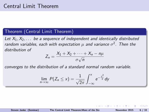
Theorem (Central Limit Theorem)

Let X1,X2, . . . be a sequence of independent and identically distributedrandom variables, each with expectation µ and variance σ2. Then thedistribution of

Zn =X1 + X2 + · · ·+ Xn − nµ

σ√

n

converges to the distribution of a standard normal random variable.

limn→∞

P(Zn ≤ x) =1√2π

∫ x

−∞e−

y2

2 dy


Central Limit Theorem Applications

The sampling distribution of the mean is approximately normal.

The distribution of experimental errors is approximately normal.

>> But why the normal distribution?


Benford’s Law

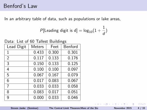
In an arbitrary table of data, such as populations or lake areas,

P[Leading digit is d] = log10(1 +1

d)

Data: List of 60 Tallest BuildingsLead Digit Meters Feet Benford

1 0.433 0.300 0.301

2 0.117 0.133 0.176

3 0.150 0.133 0.125

4 0.100 0.100 0.097

5 0.067 0.167 0.079

6 0.017 0.083 0.067

7 0.033 0.033 0.058

8 0.083 0.017 0.051

9 0.000 0.033 0.046


Benford Justification

Simon Newcomb 1881Frank Benford 1938

”Proof” arguments:

Positional number system

Densities

Scale invariance

Scale and base unbiased (Hill 1995)


Central Limit Theorem


Let X1,X2, . . . be a sequence of independent and identically distributedrandom variables, each with expectation µ and variance σ2. Then thedistribution of

Zn =X1 + X2 + · · ·+ Xn − nµ

σ√

n

converges to the distribution of a standard normal random variable.

limn→∞

P(Zn ≤ x) =1√2π

∫ x

−∞e−

y2

2 dy


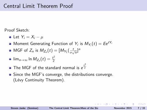
Central Limit Theorem Proof

Proof Sketch:

Let Yi = Xi − µMoment Generating Function of Yi is MYi

(t) = EetYi

MGF of Zn is MZn(t) = [MY1( tσ√n

]n

limn→∞ ln MZn(t) = t2

2

The MGF of the standard normal is et2

2

Since the MGF’s converge, the distributions converge.(Levy Continuity Theorem).


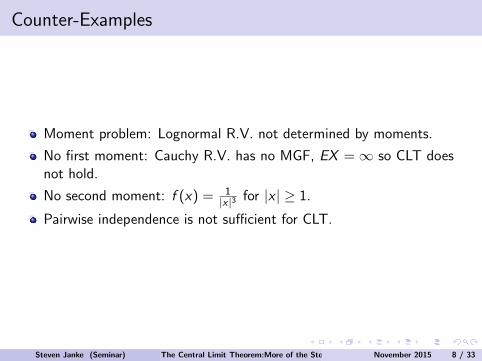
Counter-Examples

Moment problem: Lognormal R.V. not determined by moments.

No first moment: Cauchy R.V. has no MGF, EX =∞ so CLT doesnot hold.

No second moment: f (x) = 1|x |3 for |x | ≥ 1.

Pairwise independence is not sufficient for CLT.


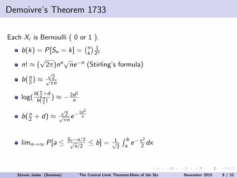
Demoivre’s Theorem 1733

Each Xi is Bernoulli ( 0 or 1 ).

b(k) = P[Sn = k] =(nk

)12n

n! ≈ (√

2π)nn√ne−n (Stirling’s formula)

b(n2 ) ≈√2√πn

log(b( n

2+d

b( n2) ) ≈ −2d2

n

b(n2 + d) ≈√2√πn

e−2d2

n

limn→∞ P[a ≤ Sn−n/2√n/2≤ b] = 1√

2

∫ ba e− x2

2 dx


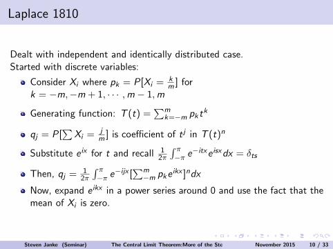
Laplace 1810

Dealt with independent and identically distributed case.Started with discrete variables:

Consider Xi where pk = P[Xi = km ] for

k = −m,−m + 1, · · · ,m − 1,m

Generating function: T (t) =∑m

k=−m pktk

qj = P[∑

Xi = jm ] is coefficient of t j in T (t)n

Substitute e ix for t and recall 12π

∫ π−π e−itxe isxdx = δts

Then, qj = 12π

∫ π−π e−ijx [

∑m−m pke ikx ]ndx

Now, expand e ikx in a power series around 0 and use the fact that themean of Xi is zero.


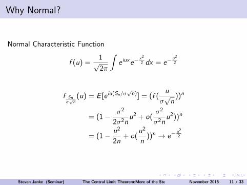
Why Normal?

Normal Characteristic Function

f (u) =1√2π

∫e iuxe−

x2

2 dx = e−u2

2

f Snσ√n(u) = E [e iu(Sn/σ

√n)] = (f (

u

σ√

n))n

= (1− σ2

2σ2nu2 + o(

σ2

σ2nu2))n

= (1− u2

2n+ o(

u2

n))n → e−

u2

2


Levy Continuity

Theorem

If distribution functions Fn converge to F , then the corresponding ch.f. fnconverge to f . Conversely, if fn converges to g continuous at 0, then Fn

converges to F .

Proof Sketch:

First direction is the Helly-Bray theorem.

The set e iux is a separating set for distribution functions.

In both directions, continuity points and mass of Fn are critical.


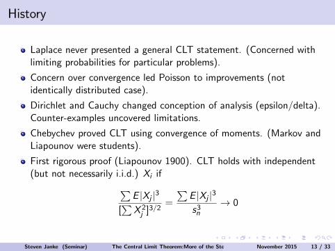
History

Laplace never presented a general CLT statement. (Concerned withlimiting probabilities for particular problems).

Concern over convergence led Poisson to improvements (notidentically distributed case).

Dirichlet and Cauchy changed conception of analysis (epsilon/delta).Counter-examples uncovered limitations.

Chebychev proved CLT using convergence of moments. (Markov andLiapounov were students).

First rigorous proof (Liapounov 1900). CLT holds with independent(but not necessarily i.i.d.) Xi if∑

E |Xj |3

[∑

X 2j ]3/2

=

∑E |Xj |3

s3n→ 0


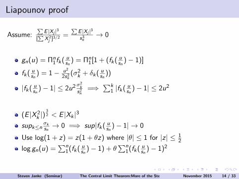
Liapounov proof

Assume:∑

E |Xj |3[∑

X 2j ]

3/2 =∑

E |Xj |3s3n

→ 0

gn(u) = Πn1fk( u

sn) = Πn

1[1 + (fk( usn

)− 1)]

fk( usn

) = 1− u2

2s2n(σ2k + δk( u

sn))

|fk( usn

)− 1| ≤ 2u2 σ2k

s2n=⇒

∑k1 |fk( u

sn)− 1| ≤ 2u2

(E |X 2k |)

32 < E |Xk |3

supk≤nσksn→ 0 =⇒ sup|fk( u

sn)− 1| → 0

Use log(1 + z) = z(1 + θz) where |θ| ≤ 1 for |z | ≤ 12

log gn(u) =∑n

1(fk( usn

)− 1) + θ∑n

1(fk( usn

)− 1)2


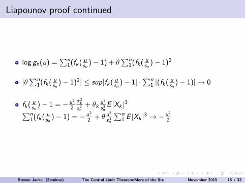
Liapounov proof continued

log gn(u) =∑n

1(fk( usn

)− 1) + θ∑n

1(fk( usn

)− 1)2

|θ∑n

1(fk( usn

)− 1)2| ≤ sup|fk( usn

)− 1| ·∑n

1 |(fk( usn

)− 1)| → 0

fk( usn

)− 1 = −u2

2σ2k

s2n+ θk

u3

s3nE |Xk |3∑n

1(fk( usn

)− 1) = −u2

2 + θ u3

s3n

∑n1 E |Xk |3 → −u2

2


Lindeberg 1922


Let the variables Xi be independent with EXi = 0 and EX 2i = σ2i . Let s be

the standard deviation of the sum S and let F be the distribution of Ss .

With Φ(x) the normal distribution, then if 1s2n

∑∫|x |≥εsn x2dFk → 0, we

havesupx|F (x)− Φ(x)| ≤ 5ε


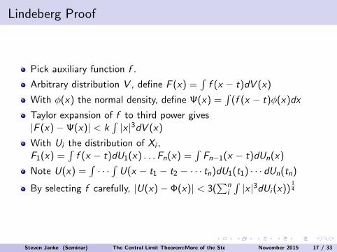
Lindeberg Proof

Pick auxiliary function f .

Arbitrary distribution V , define F (x) =∫

f (x − t)dV (x)

With φ(x) the normal density, define Ψ(x) =∫

(f (x − t)φ(x)dx

Taylor expansion of f to third power gives|F (x)−Ψ(x)| < k

∫|x |3dV (x)

With Ui the distribution of Xi ,F1(x) =

∫f (x − t)dU1(x) . . .Fn(x) =

∫Fn−1(x − t)dUn(x)

Note U(x) =∫· · ·∫

U(x − t1 − t2 − · · · tn)dU1(t1) · · · dUn(tn)

By selecting f carefully, |U(x)− Φ(x)| < 3(∑n

i

∫|x |3dUi (x))

14


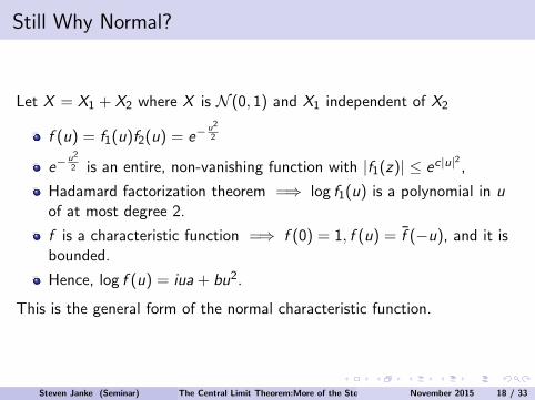
Still Why Normal?

Let X = X1 + X2 where X is N (0, 1) and X1 independent of X2

f (u) = f1(u)f2(u) = e−u2

2

e−u2

2 is an entire, non-vanishing function with |f1(z)| ≤ ec|u|2,

Hadamard factorization theorem =⇒ log f1(u) is a polynomial in uof at most degree 2.

f is a characteristic function =⇒ f (0) = 1, f (u) = f (−u), and it isbounded.

Hence, log f (u) = iua + bu2.

This is the general form of the normal characteristic function.


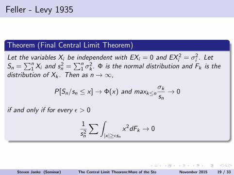
Feller - Levy 1935

Theorem (Final Central Limit Theorem)

Let the variables Xi be independent with EXi = 0 and EX 2i = σ2i . Let

Sn =∑n

1 Xi and s2n =∑n

1 σ2k . Φ is the normal distribution and Fk is the

distribution of Xk . Then as n→∞,

P[Sn/sn ≤ x ]→ Φ(x) and maxk≤nσksn→ 0

if and only if for every ε > 0

1

s2n

∑∫|x |≥εsn

x2dFk → 0


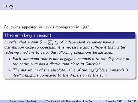
Levy

Following appeared in Levy’s monograph in 1937.

Theorem (Levy’s version)

In order that a sum S =∑

j Xj of independent variables have adistribution close to Gaussian, it is necessary and sufficient that, afterreducing medians to zero, the following conditions be satisfied.

Each summand that is not negligible compared to the dispersion ofthe entire sum has a distribution close to Gaussian.

The maximum of the absolute value of the negligible summands isitself negligible compared to the dispersion of the sum.


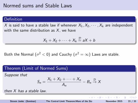
Normed sums and Stable Laws

Definition

X is said to have a stable law if whenever X1,X2, · · · ,Xk are independentwith the same distribution as X , we have

X1 + X2 + · · ·+ XkD= aX + b

Both the Normal (σ2 < 0) and Cauchy (σ2 =∞) Laws are stable.

Theorem (Limit of Normed Sums)

Suppose that

Sn =X1 + X2 + · · ·+ Xn

An− Bn

D→ X

then X has a stable law.


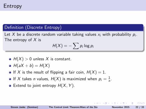
Entropy

Definition (Discrete Entropy)

Let X be a discrete random variable taking values xi with probability pi .The entropy of X is

H(X ) = −∑

pi log pi

H(X ) > 0 unless X is constant.

H(aX + b) = H(X )

If X is the result of flipping a fair coin, H(X ) = 1.

If X takes n values, H(X ) is maximized when pi = 1n .

Extend to joint entropy H(X ,Y ).


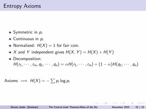
Entropy Axioms

Symmetric in pi

Continuous in pi

Normalized: H(X ) = 1 for fair coin.

X and Y independent gives H(X ,Y ) = H(X ) + H(Y )

Decomposition:H(r1, · · · , rm, q1, · · · , qn) = αH(r1, · · · , rm) + (1− α)H(q1, · · · , qn)

Axioms =⇒ H(X ) = −∑

pi log pi


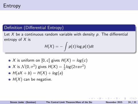
Entropy

Definition (Differential Entropy)

Let X be a continuous random variable with density p. The differentialentropy of X is

H(X ) = −∫

p(t) log p(t)dt

X is uniform on [0, c] gives H(X ) = log(c)

X is N (0, σ2) gives H(X ) = 12 log(2πeσ2)

H(aX + b) = H(X ) + log(a)

H(X ) can be negative.


Entropy

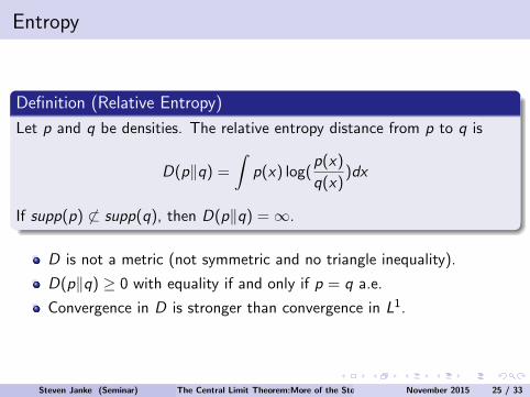
Definition (Relative Entropy)

Let p and q be densities. The relative entropy distance from p to q is

D(p‖q) =

∫p(x) log(

p(x)

q(x))dx

If supp(p) 6⊂ supp(q), then D(p‖q) =∞.

D is not a metric (not symmetric and no triangle inequality).

D(p‖q) ≥ 0 with equality if and only if p = q a.e.

Convergence in D is stronger than convergence in L1.


Entropy

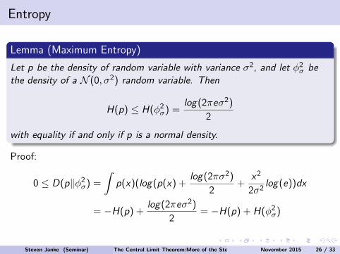
Lemma (Maximum Entropy)

Let p be the density of random variable with variance σ2, and let φ2σ bethe density of a N (0, σ2) random variable. Then

H(p) ≤ H(φ2σ) =log(2πeσ2)

2

with equality if and only if p is a normal density.

Proof:

0 ≤ D(p‖φ2σ) =

∫p(x)(log(p(x) +

log(2πσ2)

2+

x2

2σ2log(e))dx

= −H(p) +log(2πeσ2)

2= −H(p) + H(φ2σ)


Second Law of Thermodynamics

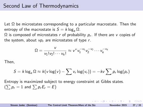
Let Ω be microstates corresponding to a particular macrostate. Then theentropy of the macrostate is S = k loge Ω.Ω is composed of microstates r of probability pr . If there are v copies ofthe system, about vpr are microstates of type r .

Ω =v

v1!v2! · · · vk !≈ v vv−v11 v−v22 · · · v−vkk

Then,

S = k loge Ω ≈ k(v log(v)−∑

vr log(vr )) = −kv∑

pr log(pr )

Entropy is maximized subject to energy constraint at Gibbs states.(∑

pr = 1 and∑

prEr = E )


Fisher Information

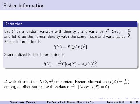
Definition

Let Y be a random variable with density g and variance σ2. Set ρ = g ′

gand let φ be the normal density with the same mean and variance as Y .Fisher Information is

I (Y ) = E [(ρ(Y ))2]

Standardized Fisher Information is

J(Y ) = σ2E [(ρ(Y )− ρφ(Y ))2]

Z with distribution N (0, σ2) minimizes Fisher information (I (Z ) = 1σ2 )

among all distributions with variance σ2. (Note: J(Z ) = 0)


Fisher Information Properties

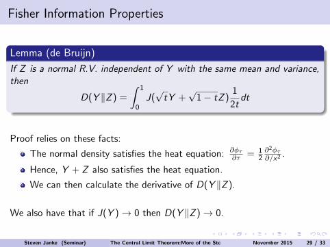
Lemma (de Bruijn)

If Z is a normal R.V. independent of Y with the same mean and variance,then

D(Y ‖Z ) =

∫ 1

0J(√

tY +√

1− tZ )1

2tdt

Proof relies on these facts:

The normal density satisfies the heat equation: ∂φτ∂τ = 1

2∂2φτ∂/x2

.

Hence, Y + Z also satisfies the heat equation.

We can then calculate the derivative of D(Y ‖Z ).

We also have that if J(Y )→ 0 then D(Y ‖Z )→ 0.



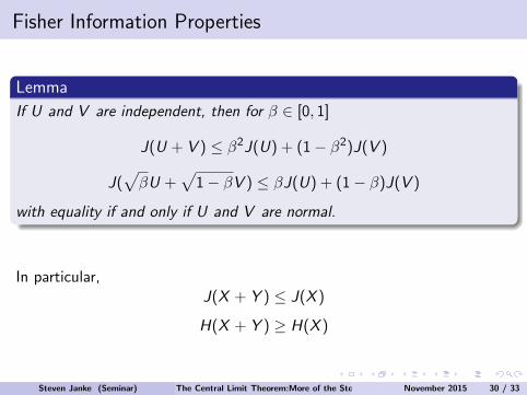
Lemma

If U and V are independent, then for β ∈ [0, 1]

J(U + V ) ≤ β2J(U) + (1− β2)J(V )

J(√βU +

√1− βV ) ≤ βJ(U) + (1− β)J(V )

with equality if and only if U and V are normal.

In particular,J(X + Y ) ≤ J(X )

H(X + Y ) ≥ H(X )



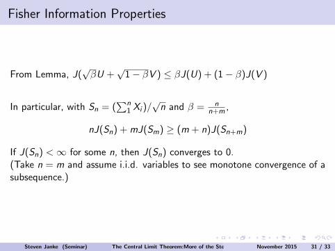
From Lemma, J(√βU +

√1− βV ) ≤ βJ(U) + (1− β)J(V )

In particular, with Sn = (∑n

1 Xi )/√

n and β = nn+m ,

nJ(Sn) + mJ(Sm) ≥ (m + n)J(Sn+m)

If J(Sn) <∞ for some n, then J(Sn) converges to 0.(Take n = m and assume i.i.d. variables to see monotone convergence of asubsequence.)


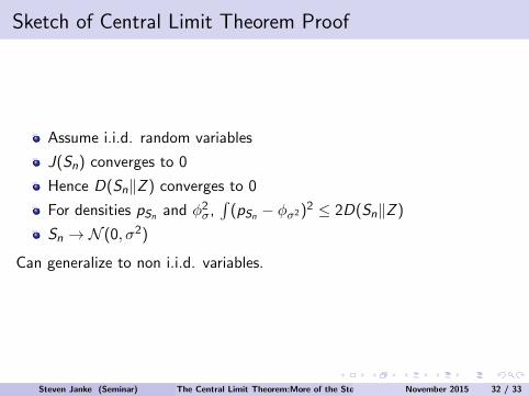
Sketch of Central Limit Theorem Proof

Assume i.i.d. random variables

J(Sn) converges to 0

Hence D(Sn‖Z ) converges to 0

For densities pSn and φ2σ,∫

(pSn − φσ2)2 ≤ 2D(Sn‖Z )

Sn → N (0, σ2)

Can generalize to non i.i.d. variables.


Conclusions

Assume errors are ”uniformally asymptotically negligible” (no onedominates).

Assume independent errors with distributions that have secondmoments.

Normalize the sum with mean and variance.

Then the limit is a standard normal distribution.

Normal distribution is stable (”infinitely divisible”). (X = X1 + X2)

Normal distribution maximizes entropy.

Convolution (adding R.V.’s) increases entropy.


The Central Limit Theorem: More of the Story

Documents

Transcript of The Central Limit Theorem: More of the Story