1

LabCPS

School of Computing, Informatics and Decision System Engineering

Arizona State University

fainekos at asu edu

http://www.public.asu.edu/~gfaineko

Georgios Fainekos

Temporal Logic Testing for Hybrid Systems

2

LabCPS

“A design without specifications cannot be right or wrong, it can only be surprising!”*

*Lee & Seshia, Introduction to Embedded Systems: A Cyber-Physical Systems Approach, 2011 paraphrased from Boebert & Kain: Proving a computer system secure. Scientific Honeyweller, 6(2), 18–27, 1985

3

LabCPS

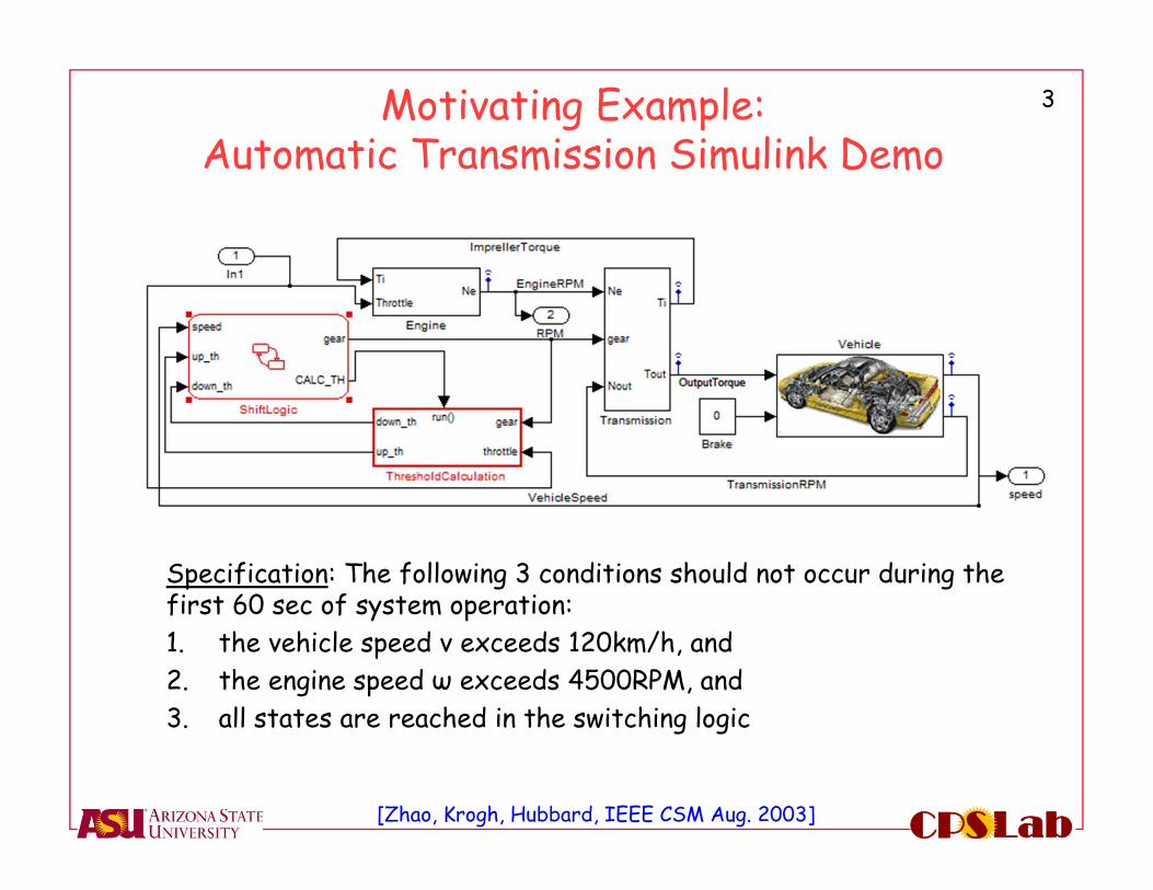
Motivating Example: Automatic Transmission Simulink Demo

Specification: The following 3 conditions should not occur during the first 60 sec of system operation:1. the vehicle speed v exceeds 120km/h, and 2. the engine speed ω exceeds 4500RPM, and3. all states are reached in the switching logic

[Zhao, Krogh, Hubbard, IEEE CSM Aug. 2003]

4

LabCPS

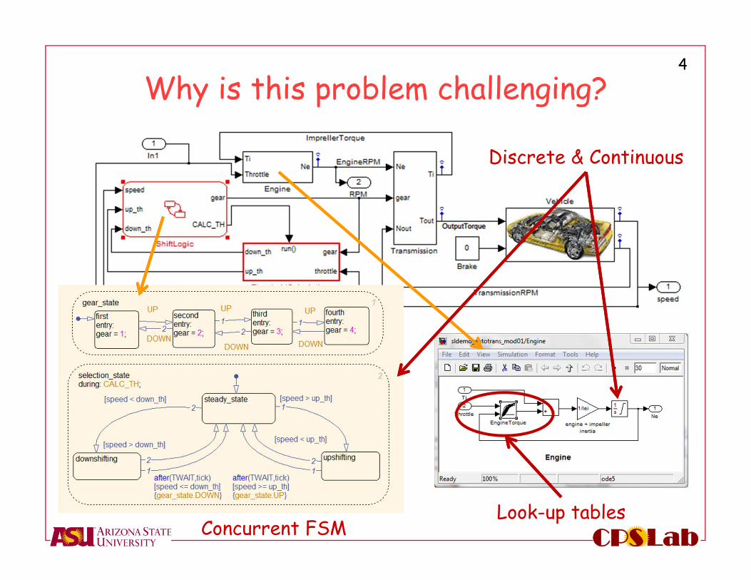
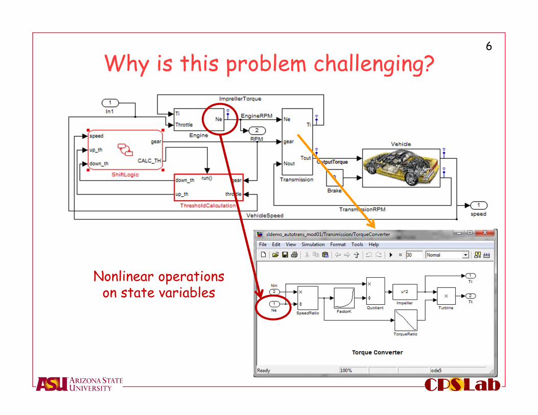
Why is this problem challenging?

Concurrent FSMLook-up tables

Discrete & Continuous

5

LabCPS

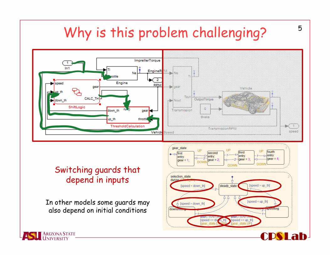
Why is this problem challenging?

Switching guards that depend in inputs

In other models some guards may also depend on initial conditions

6

LabCPS

Why is this problem challenging?

Nonlinear operations on state variables

7

LabCPS

In summary• Nonlinear ODEs with 2 state variables• 3 look-up tables and 3 look-up 2D tables • A Stateflow chart: two concurrent FSM with 4 and 3 states

If you would like to get real, in simplified models you will expect ~100 state variables (both continuous & discrete time)

8

LabCPS

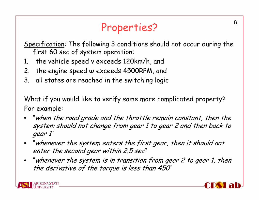
Properties?Specification: The following 3 conditions should not occur during the

first 60 sec of system operation:1. the vehicle speed v exceeds 120km/h, and 2. the engine speed ω exceeds 4500RPM, and3. all states are reached in the switching logic

What if you would like to verify some more complicated property?For example:• “when the road grade and the throttle remain constant, then the

system should not change from gear 1 to gear 2 and then back to gear 1”

• “whenever the system enters the first gear, then it should not enter the second gear within 2.5 sec”

• “whenever the system is in transition from gear 2 to gear 1, then the derivative of the torque is less than 450”

9

LabCPS

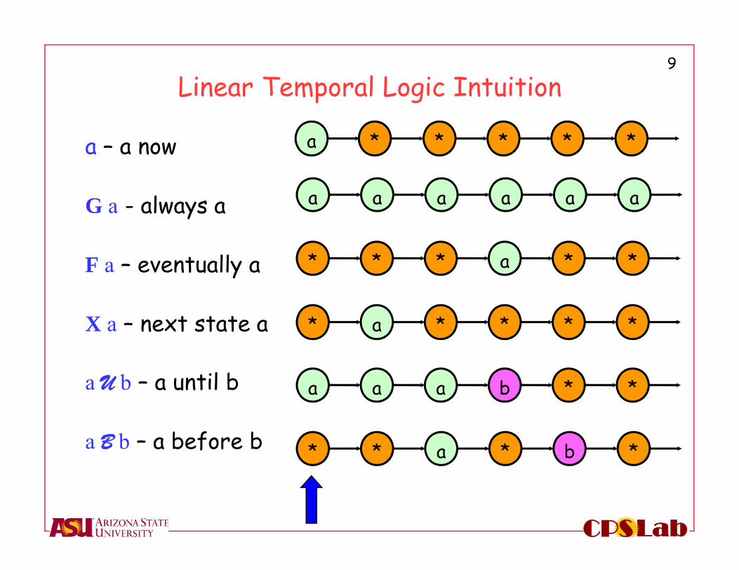
Linear Temporal Logic Intuition

a – a now

G a - always a

F a – eventually a

X a – next state a

a U b – a until b

a B b – a before b

a a a a aa

* * a * **

a * * * **

a a b * *a

* a * b **

a * * * **

10

LabCPS

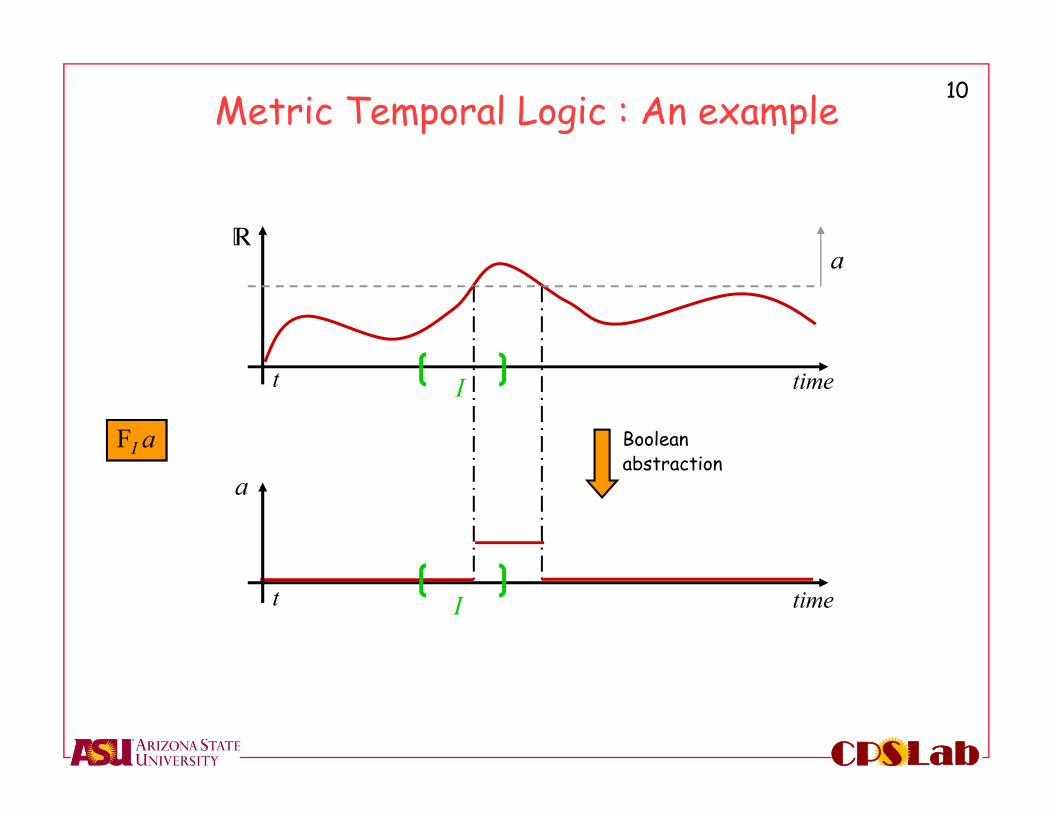
Metric Temporal Logic : An example

FI a

time

a

Booleanabstraction

a

time

I

I

t

t

R

11

LabCPS

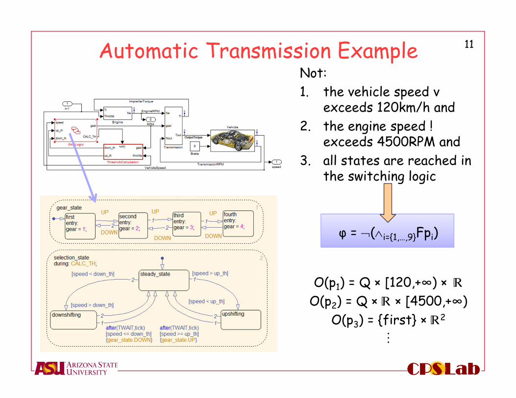
Automatic Transmission ExampleNot:1. the vehicle speed v

exceeds 120km/h and2. the engine speed !

exceeds 4500RPM and3. all states are reached in

the switching logic

φ = (i={1,…,9}Fpi)

O(p1) = Q × [120,+∞) × R

O(p2) = Q × R × [4500,+∞)O(p3) = {first} × R2

ª

12

LabCPS

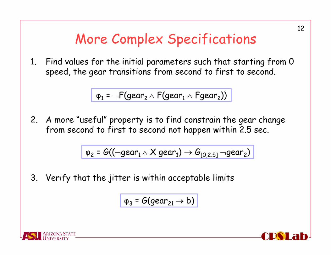
More Complex Specifications1. Find values for the initial parameters such that starting from 0

speed, the gear transitions from second to first to second.

2. A more “useful” property is to find constrain the gear change from second to first to second not happen within 2.5 sec.

3. Verify that the jitter is within acceptable limits

φ1 = F(gear2 F(gear1 Fgear2))

φ2 = G((gear1 X gear1) G[0,2.5] gear2)

φ3 = G(gear21 b)

13

LabCPS

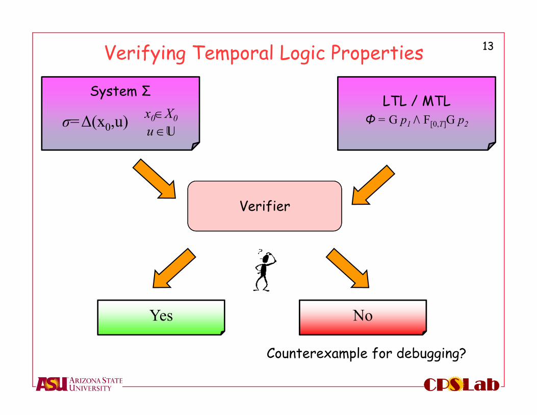
Verifying Temporal Logic Properties

LTL / MTLΦ = G p1 ⁄ F[0,Τ]G p2

System Σx0X0u U

Yes

Verifier

σ=Δ(x0,u)

No

Counterexample for debugging?

14

LabCPS

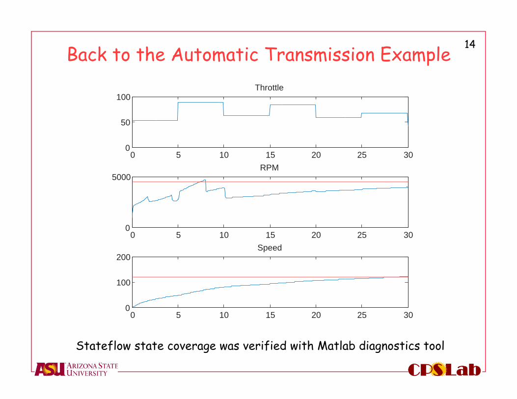
Back to the Automatic Transmission Example

0 5 10 15 20 25 300

50

100Throttle

0 5 10 15 20 25 300

5000RPM

0 5 10 15 20 25 300

100

200Speed

Stateflow state coverage was verified with Matlab diagnostics tool

15

LabCPS

This talk ...

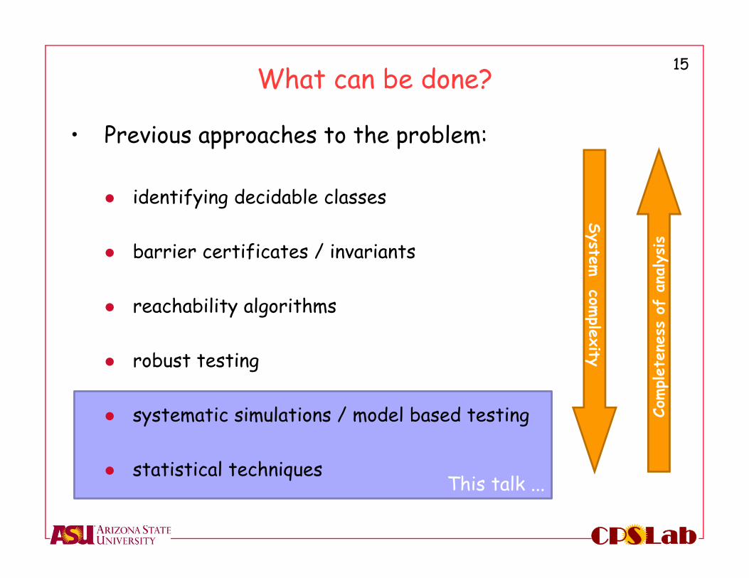
What can be done?

• Previous approaches to the problem:

identifying decidable classes

barrier certificates / invariants

reachability algorithms

robust testing

systematic simulations / model based testing

statistical techniques

System com

plexity

Complet

enes

s of

ana

lysis

16

LabCPS

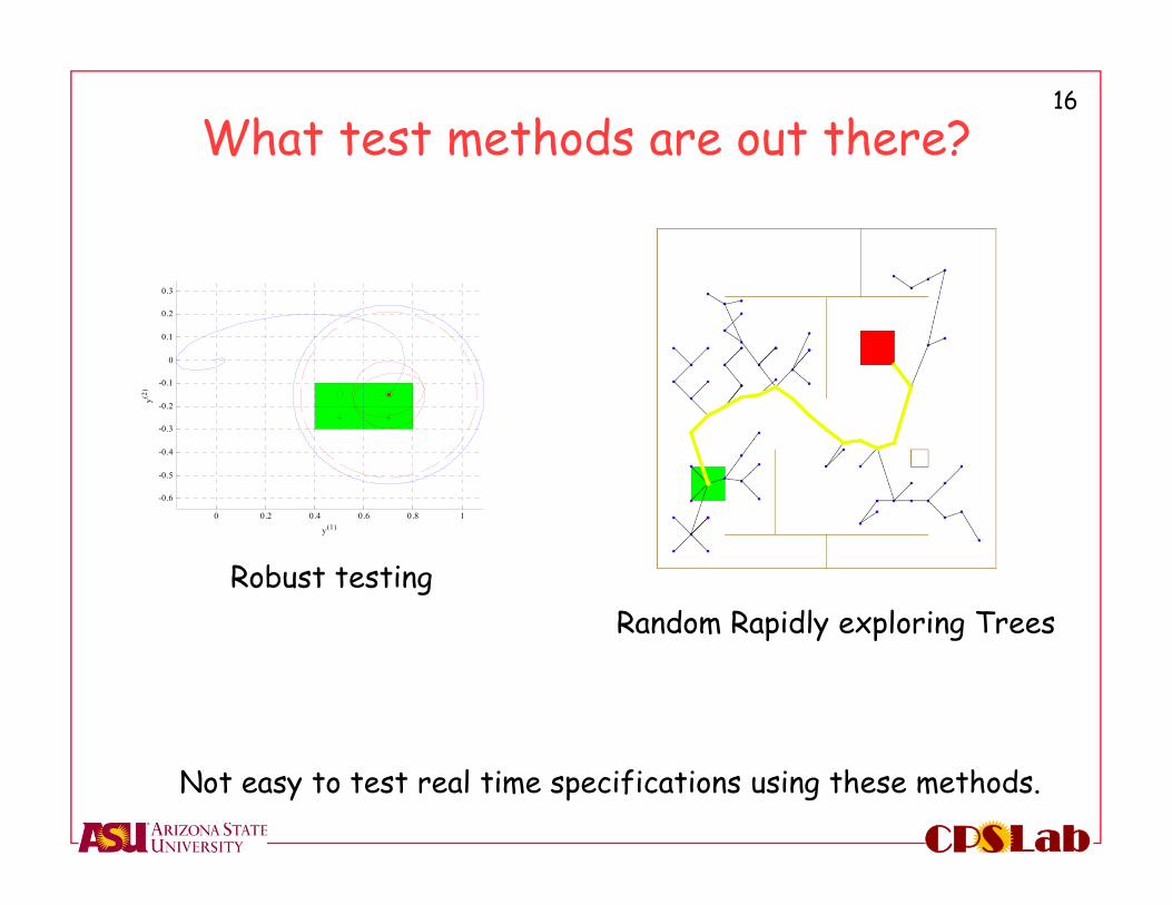
What test methods are out there?

0 0.2 0.4 0.6 0.8 1

-0.6

-0.5

-0.4

-0.3

-0.2

-0.1

0

0.1

0.2

0.3

y(1)

y(2)

Robust testingRandom Rapidly exploring Trees

Not easy to test real time specifications using these methods.

17

LabCPS

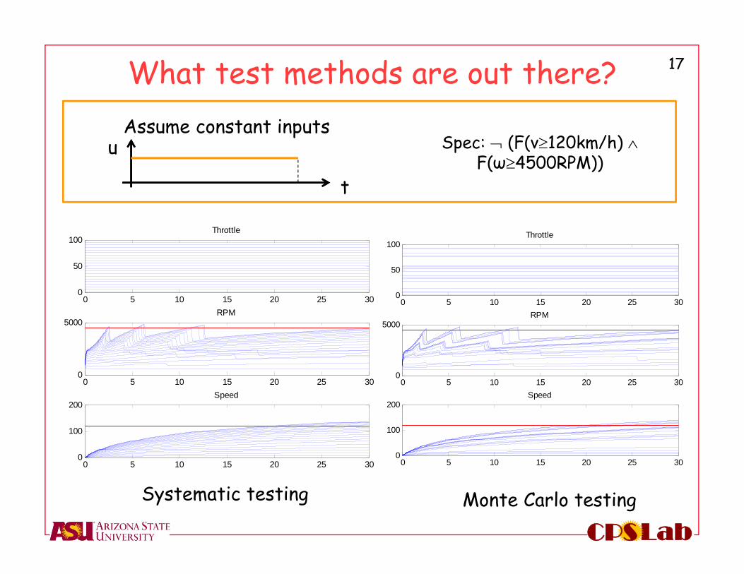
What test methods are out there?

0 5 10 15 20 25 300

50

100Throttle

0 5 10 15 20 25 300

5000RPM

0 5 10 15 20 25 300

100

200Speed

t

uAssume constant inputs

Systematic testing

0 5 10 15 20 25 300

50

100Throttle

0 5 10 15 20 25 300

5000RPM

0 5 10 15 20 25 300

100

200Speed

Monte Carlo testing

Spec: (F(v120km/h) F(ω4500RPM))

18

LabCPS

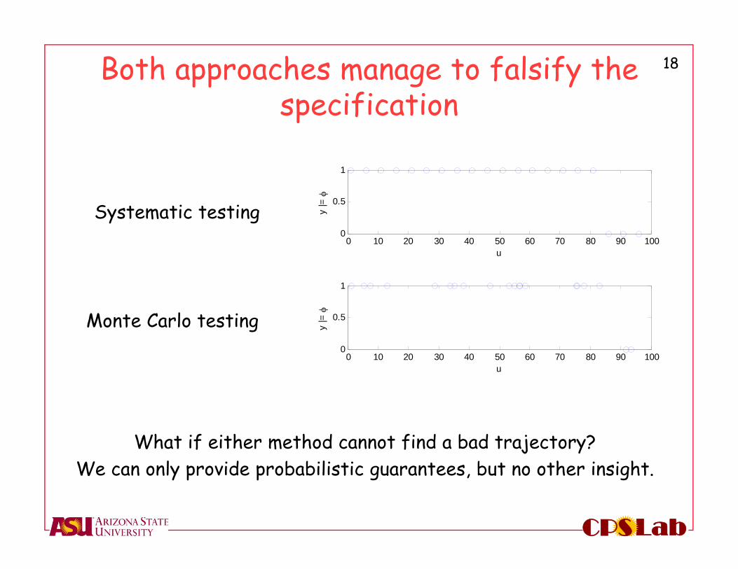
Both approaches manage to falsify the specification

0 10 20 30 40 50 60 70 80 90 1000

0.5

1

u

y |=

Monte Carlo testing

0 10 20 30 40 50 60 70 80 90 1000

0.5

1

u

y |=

Systematic testing

What if either method cannot find a bad trajectory?We can only provide probabilistic guarantees, but no other insight.

19

LabCPS

0 2 4 6 8 10-15

-10

-5

0

5

10

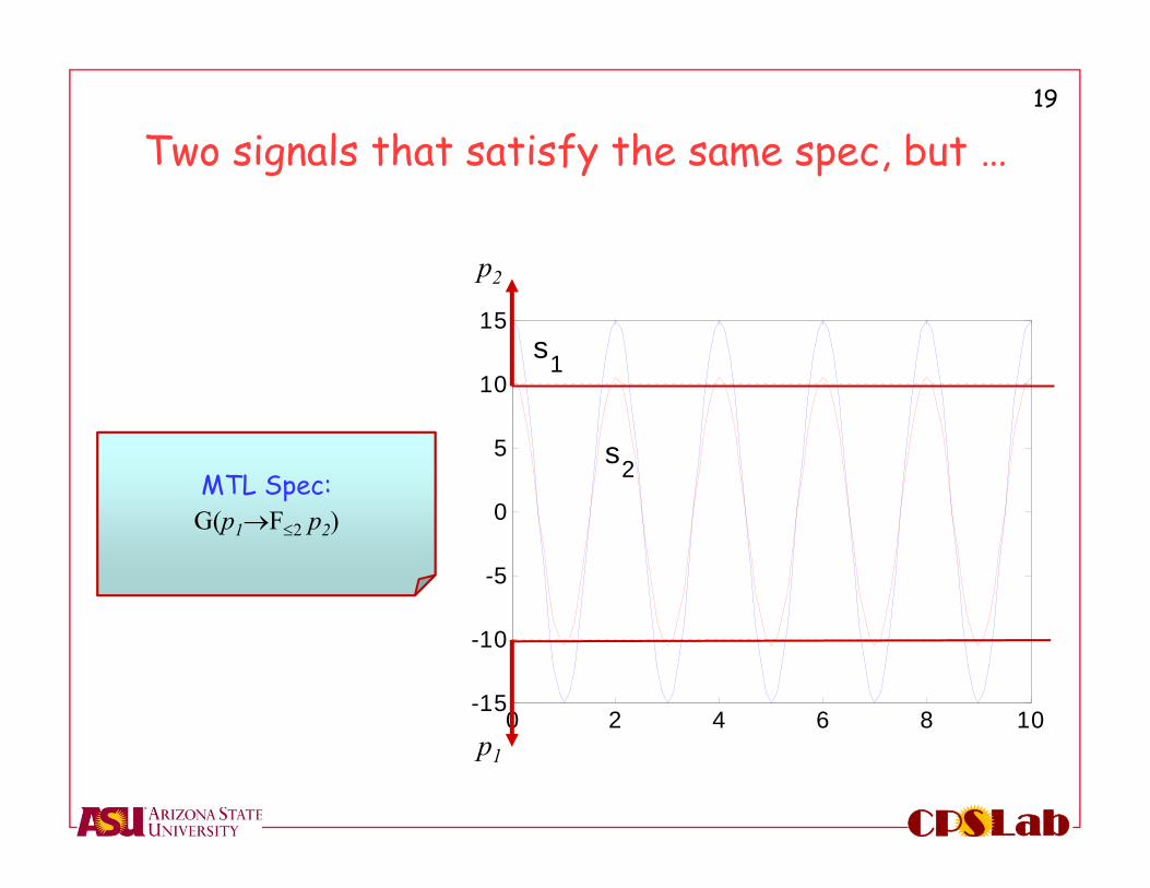
15s1

s2 MTL Spec:

G(p1F2 p2)

p2

p1

Two signals that satisfy the same spec, but …

20

LabCPS

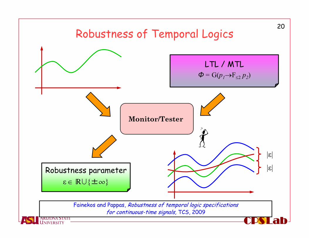
Robustness of Temporal Logics

LTL / MTLΦ = G(p1F2 p2)

Monitor/Tester

Robustness parameterε R»{±¶}

|ε|

|ε|

Fainekos and Pappas, Robustness of temporal logic specifications for continuous-time signals, TCS, 2009

21

LabCPS

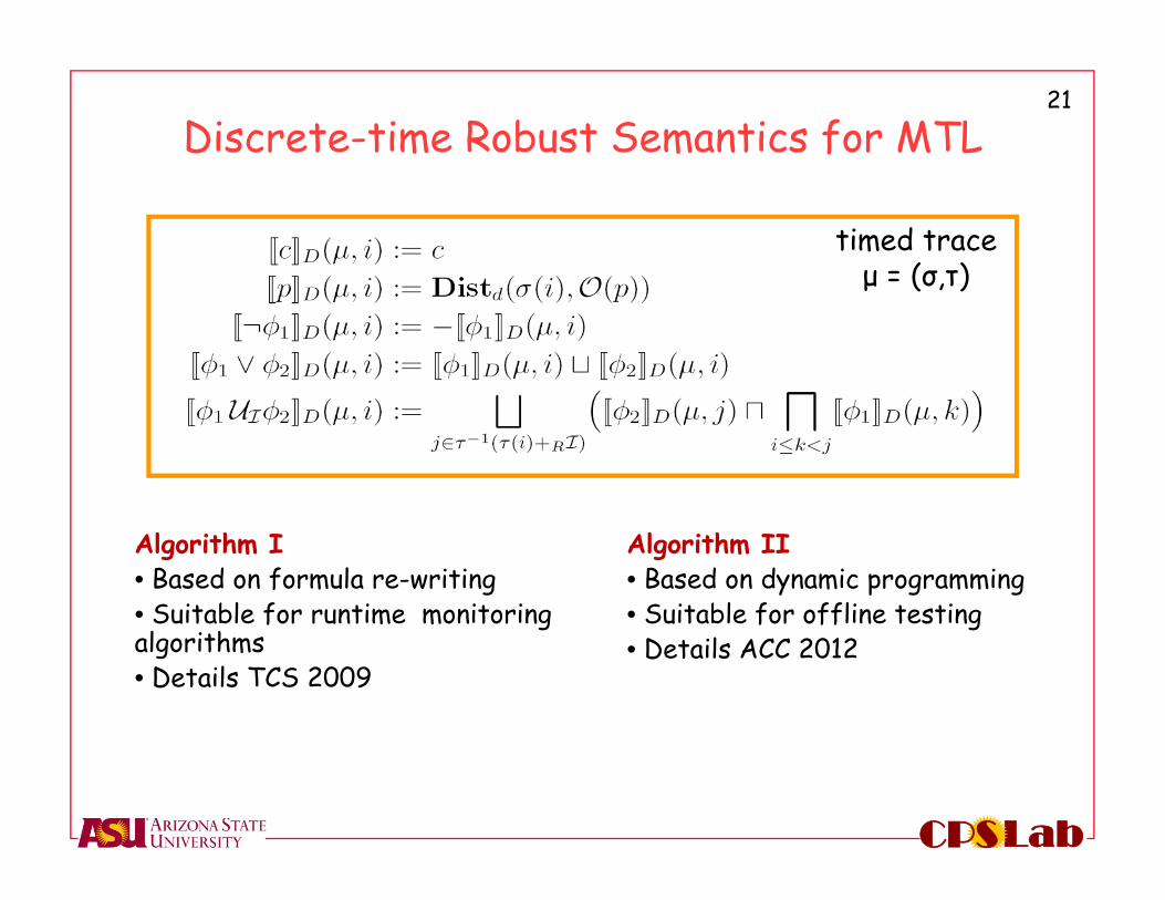
Discrete-time Robust Semantics for MTL

Algorithm I• Based on formula re-writing• Suitable for runtime monitoring algorithms • Details TCS 2009

timed traceμ = (σ,τ)

Algorithm II• Based on dynamic programming• Suitable for offline testing• Details ACC 2012

22

LabCPS

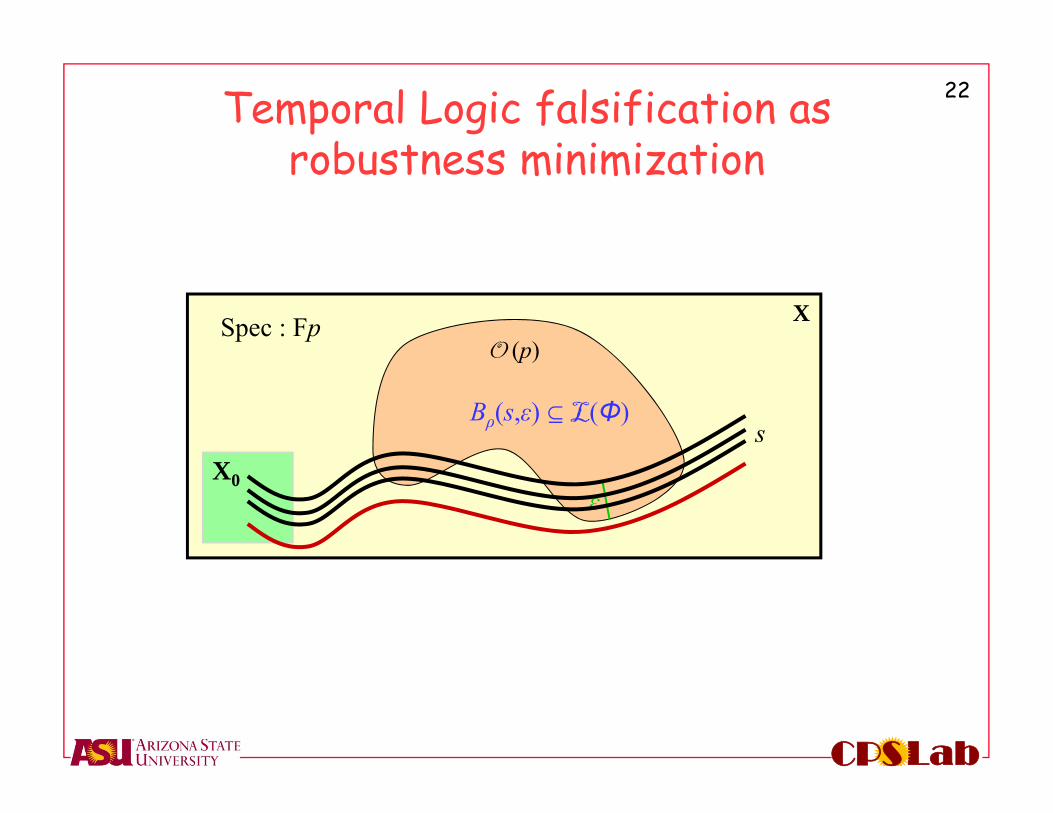
XSpec : FpO (p)

Temporal Logic falsification as robustness minimization

ε

Bρ(s,ε) Œ L(Φ)s

X0

23

LabCPS

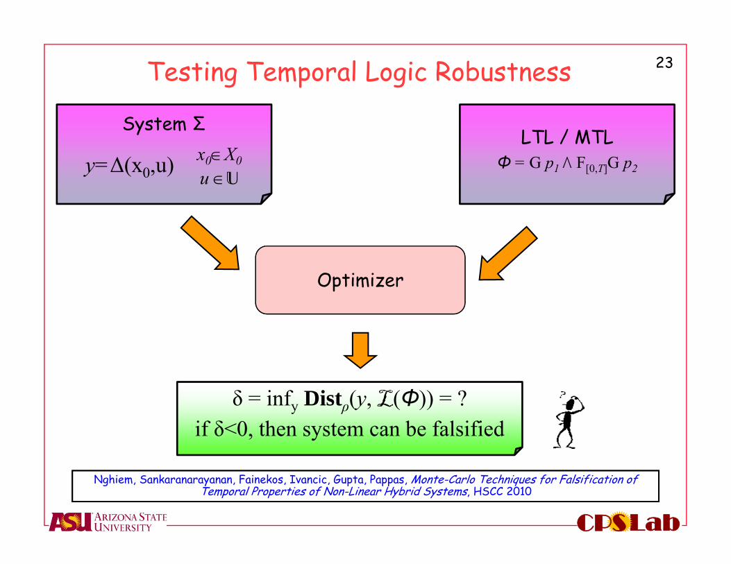
Testing Temporal Logic Robustness

LTL / MTLΦ = G p1 ⁄ F[0,Τ]G p2

System Σx0X0u U

δ = infy Distρ(y, L(Φ)) = ?if δ<0, then system can be falsified

Optimizer

Nghiem, Sankaranarayanan, Fainekos, Ivancic, Gupta, Pappas, Monte-Carlo Techniques for Falsification of Temporal Properties of Non-Linear Hybrid Systems, HSCC 2010

y=Δ(x0,u)

24

LabCPS

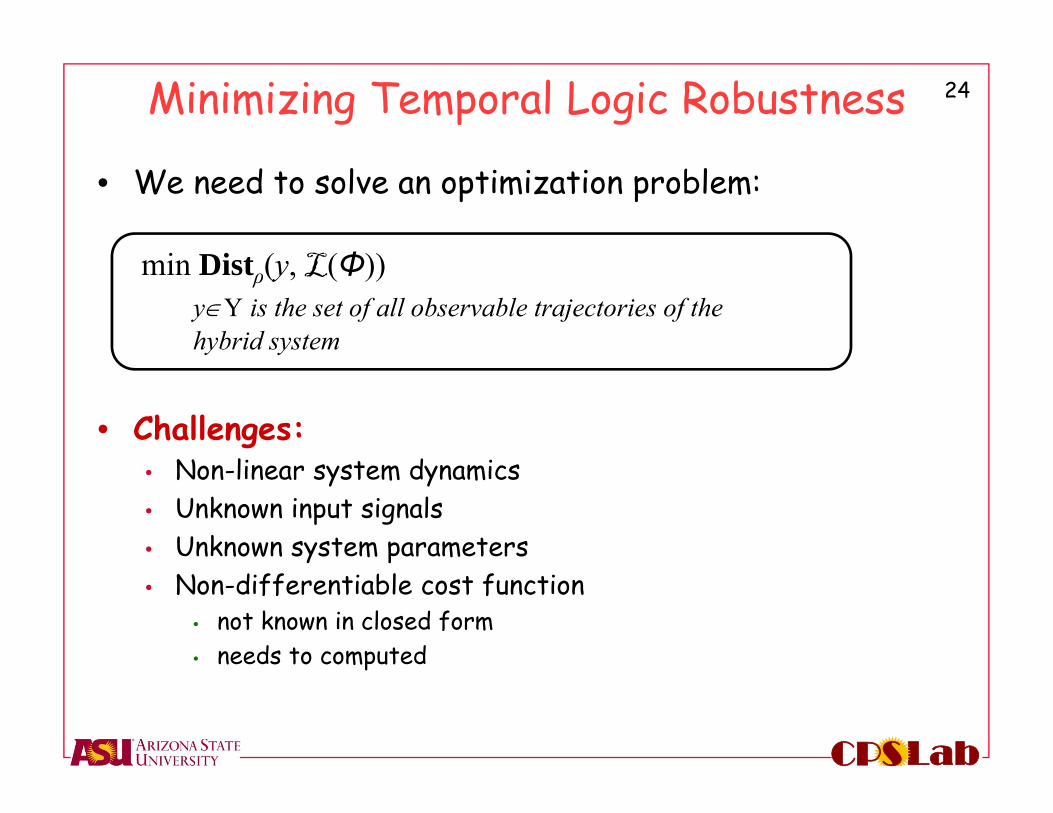
Minimizing Temporal Logic Robustness

• We need to solve an optimization problem:

min Distρ(y, L(Φ)) yY is the set of all observable trajectories of the hybrid system

• Challenges:• Non-linear system dynamics• Unknown input signals • Unknown system parameters• Non-differentiable cost function

• not known in closed form• needs to computed

25

LabCPS

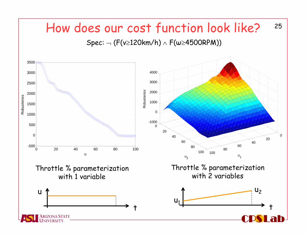
How does our cost function look like?

020

4060

80100

020

4060

80100

-1000

0

1000

2000

3000

4000

u1u2

Rob

uste

nss

Throttle % parameterization with 2 variables

tu1

0 20 40 60 80 100-500

0

500

1000

1500

2000

2500

3000

3500

u

Rob

uste

nss

Throttle % parameterization with 1 variable

t

u

Spec: (F(v120km/h) F(ω4500RPM))

u2

26

LabCPS

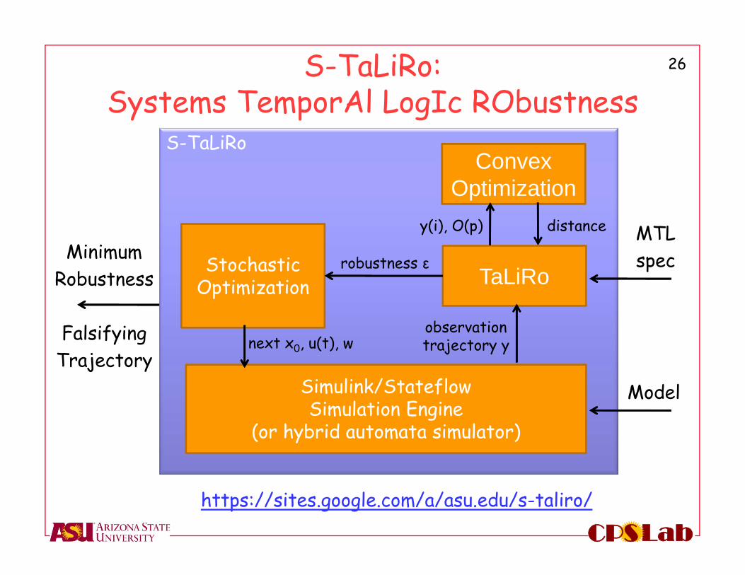
S-TaLiRo

S-TaLiRo: Systems TemporAl LogIc RObustness

Simulink/StateflowSimulation Engine

(or hybrid automata simulator)

TaLiRo

ConvexOptimization

Stochastic Optimization

MTLspec

Model

MinimumRobustness

FalsifyingTrajectory

https://sites.google.com/a/asu.edu/s-taliro/

observationtrajectory y

robustness ε

y(i), O(p) distance

next x0, u(t), w

27

LabCPS

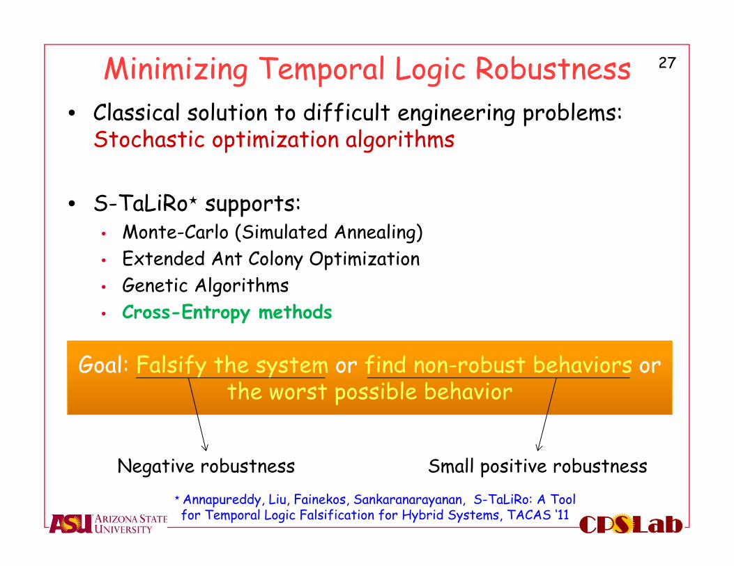
Goal: Falsify the system or find non-robust behaviors or the worst possible behavior

Minimizing Temporal Logic Robustness• Classical solution to difficult engineering problems:

Stochastic optimization algorithms

• S-TaLiRoø supports:• Monte-Carlo (Simulated Annealing)• Extended Ant Colony Optimization• Genetic Algorithms• Cross-Entropy methods

Negative robustness Small positive robustnessø Annapureddy, Liu, Fainekos, Sankaranarayanan, S-TaLiRo: A Tool for Temporal Logic Falsification for Hybrid Systems, TACAS ‘11

28

LabCPS

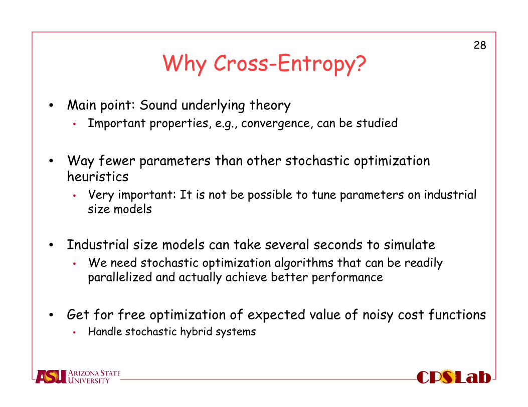
Why Cross-Entropy?

• Main point: Sound underlying theory• Important properties, e.g., convergence, can be studied

• Way fewer parameters than other stochastic optimization heuristics

• Very important: It is not be possible to tune parameters on industrial size models

• Industrial size models can take several seconds to simulate• We need stochastic optimization algorithms that can be readily

parallelized and actually achieve better performance

• Get for free optimization of expected value of noisy cost functions• Handle stochastic hybrid systems

29

LabCPS

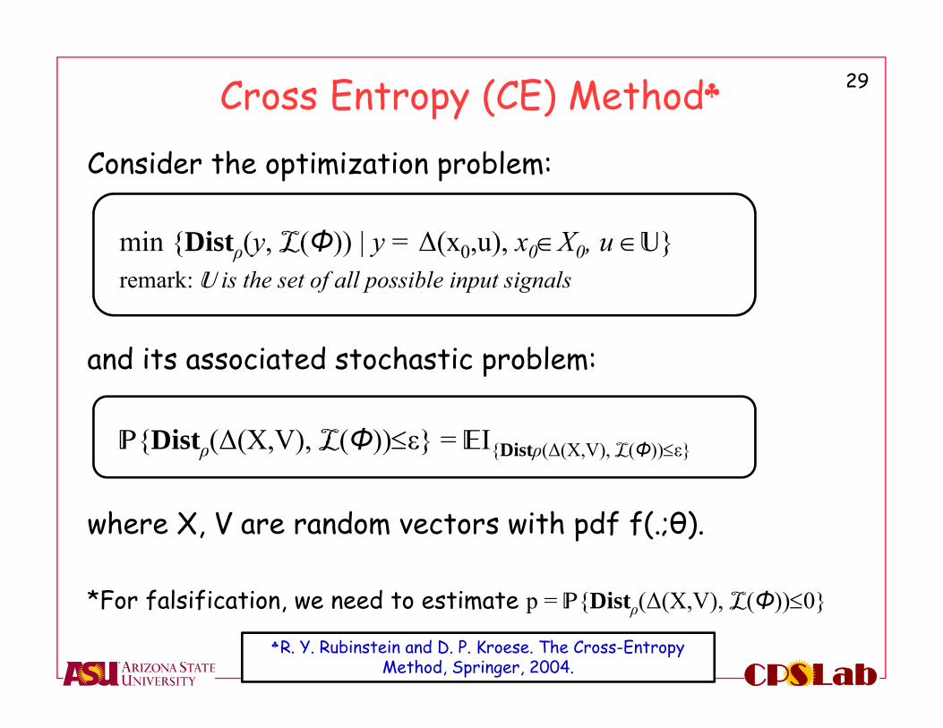
Cross Entropy (CE) Method

Consider the optimization problem:

min {Distρ(y, L(Φ)) | y = Δ(x0,u), x0X0, u U}remark: U is the set of all possible input signals

and its associated stochastic problem:

P{Distρ(Δ(X,V), L(Φ))ε} = EΙ{Distρ(Δ(X,V), L(Φ))ε}

where X, V are random vectors with pdf f(.;θ).

*For falsification, we need to estimate p = P{Distρ(Δ(X,V), L(Φ))0}

R. Y. Rubinstein and D. P. Kroese. The Cross-EntropyMethod, Springer, 2004.

30

LabCPS

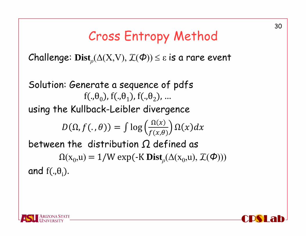
Cross Entropy MethodChallenge: Distρ(Δ(X,V), L(Φ)) ε is a rare event

Solution: Generate a sequence of pdfsf .,θ0 ,f .,θ1 ,f .,θ2 ,…

using the Kullback-Leibler divergence

Ω, . , log,

Ω

between the distribution Ω defined asΩ(x0,u) 1/Wexp ‐KDistρ(Δ(x0,u), L(Φ)))

and f .,θi .

31

LabCPS

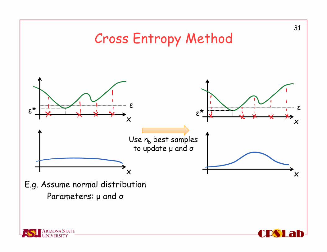
Cross Entropy Method

ε*xε

xE.g. Assume normal distribution

Parameters: μ and σ

Use nb best samples to update μ and σ

xε* ε

x

32

LabCPS

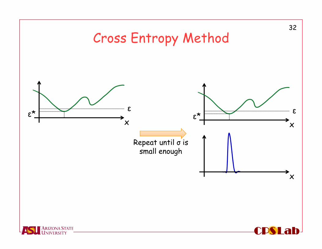
Cross Entropy Method

ε*xε

Repeat until σ is small enough

xε* ε

x

33

LabCPS

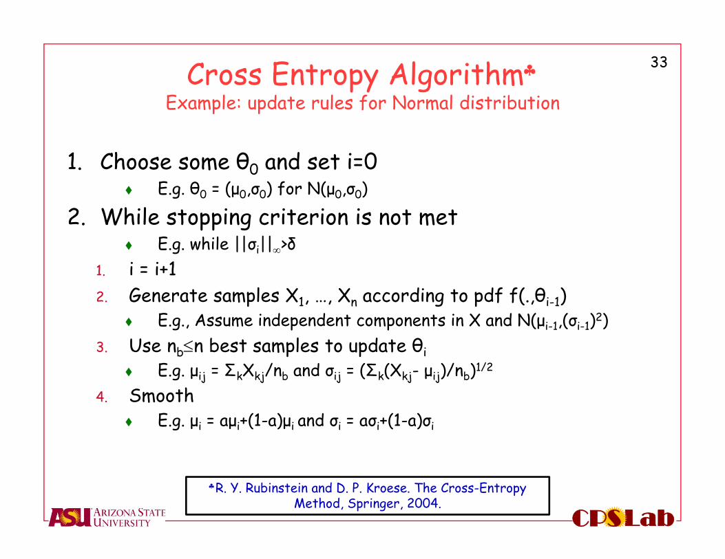
Cross Entropy Algorithm

Example: update rules for Normal distribution

1. Choose some θ0 and set i=0 E.g. θ0 = (μ0,σ0) for N(μ0,σ0)

2. While stopping criterion is not met E.g. while ||σi||>δ

1. i = i+12. Generate samples X1, …, Xn according to pdf f(.,θi-1)

E.g., Assume independent components in X and N(μi-1,(σi-1)2)3. Use nbn best samples to update θi

E.g. μij = ΣkXkj/nb and σij = (Σk(Xkj- μij)/nb)1/2

4. Smooth E.g. μi = aμi+(1-a)μi and σi = aσi+(1-a)σi

R. Y. Rubinstein and D. P. Kroese. The Cross-EntropyMethod, Springer, 2004.

34

LabCPS

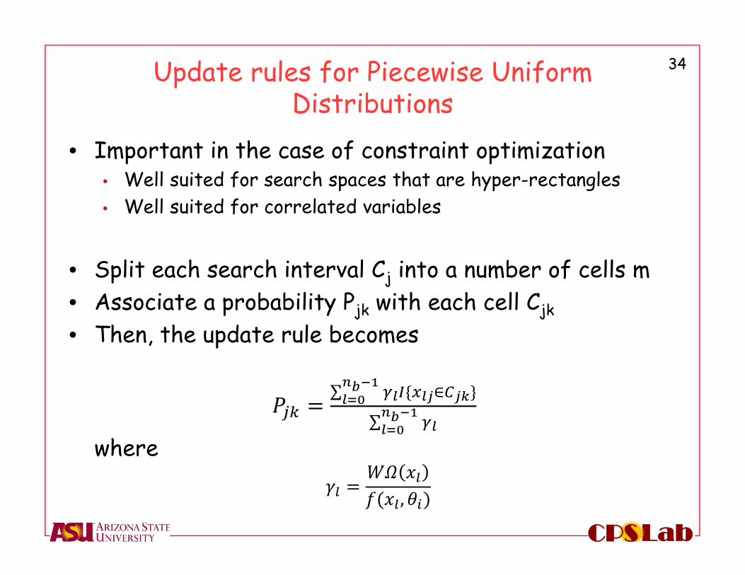
Update rules for Piecewise Uniform Distributions

• Important in the case of constraint optimization• Well suited for search spaces that are hyper-rectangles• Well suited for correlated variables

• Split each search interval Cj into a number of cells m• Associate a probability Pjk with each cell Cjk

• Then, the update rule becomes

∑ ∈

∑

where

,

35

LabCPS

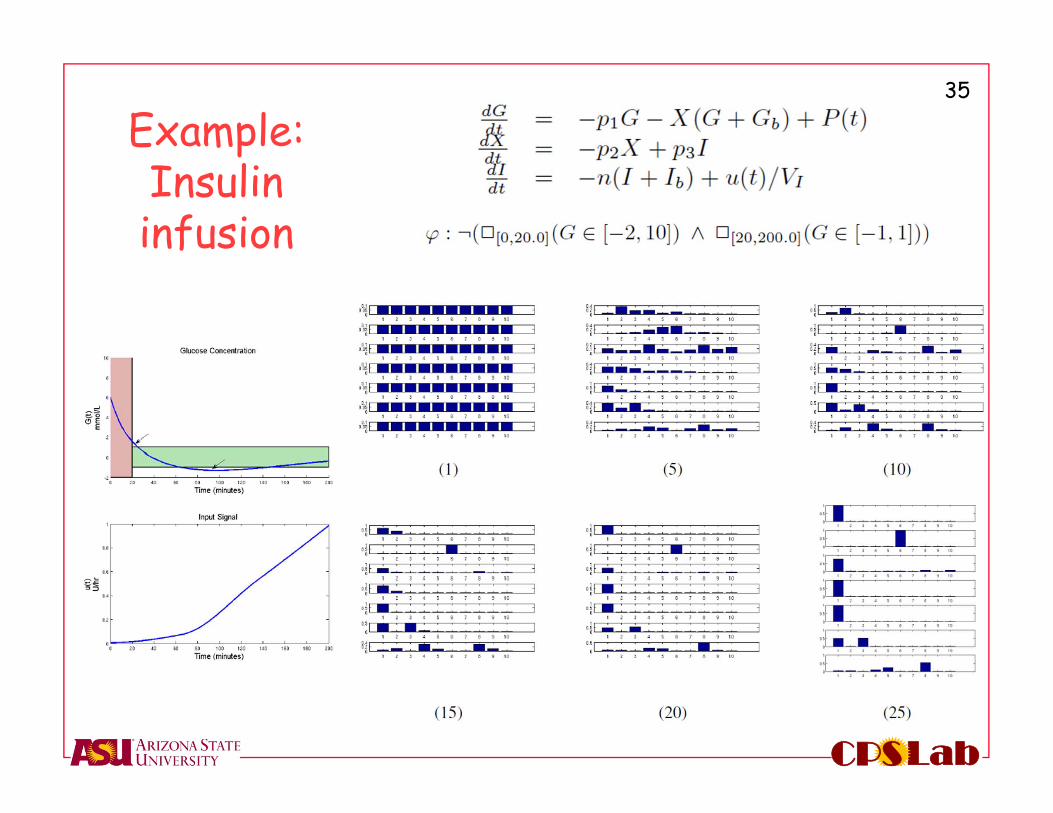
Example: Insulin infusion

36

LabCPS

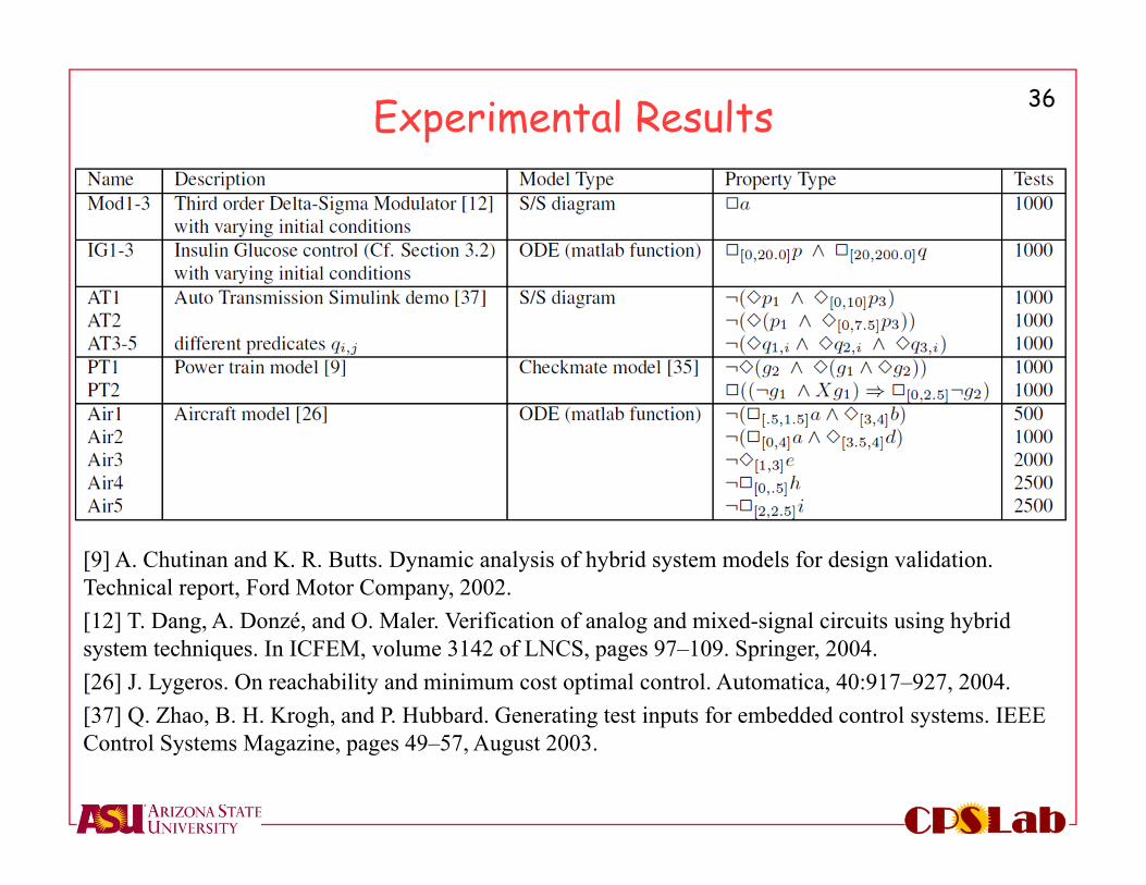
Experimental Results

[9] A. Chutinan and K. R. Butts. Dynamic analysis of hybrid system models for design validation. Technical report, Ford Motor Company, 2002.[12] T. Dang, A. Donzé, and O. Maler. Verification of analog and mixed-signal circuits using hybrid system techniques. In ICFEM, volume 3142 of LNCS, pages 97–109. Springer, 2004.[26] J. Lygeros. On reachability and minimum cost optimal control. Automatica, 40:917–927, 2004.[37] Q. Zhao, B. H. Krogh, and P. Hubbard. Generating test inputs for embedded control systems. IEEE Control Systems Magazine, pages 49–57, August 2003.

37

LabCPS

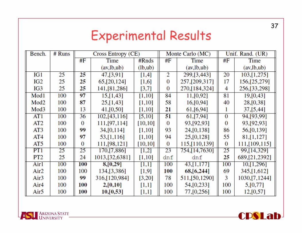
Experimental Results

38

LabCPS

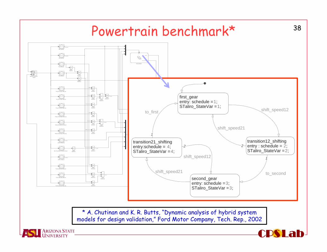
Powertrain benchmark*

* A. Chutinan and K. R. Butts, “Dynamic analysis of hybrid system models for design validation,” Ford Motor Company, Tech. Rep., 2002

shift_speed21

C*x <= d

shift_speed12

C*x <= d

shift_scheduler

schedule

STaliro_StateVar

inert21_c1slip_dz

C*x <= d

inert12_c2slip_neg

C*x <= d

first_c2slip_pos

C*x <= d

first_c2slip_dz

C*x <= d

dynamic mode selection

mode

gear

reset

abs_Tc2_gt_abs_RTc2updn_2nd_tg1

C*x <= d

To Workspace1

events

To Workspace

states

Tc2_lt1_tq21_tg1_c2slip_pos

C*x <= d

Tc2_lt1_tq21_tg1_c2slip_neg

C*x <= d

Tc2_lt1_tq21_tg1_c2slip_dz

C*x <= d

Tc2_gt1_1st_tg2_c2slip_pos

C*x <= d

Tc2_gt1_1st_tg2_c2slip_neg

C*x <= d

Tc2_gt1_1st_tg2_c2slip_dz

C*x <= d

Switched ContinuousSystem

RTsp1_lt0_tq12_tg2_c2slip_pos

C*x <= d

RTsp1_lt0_tq12_tg2_c2slip_neg

C*x <= d

RTsp1_lt0_tq12_tg2_c2slip_dz

C*x <= d

LogicalOperator9

AND

LogicalOperator8

AND

LogicalOperator7

AND

LogicalOperator6

AND

LogicalOperator5

AND

LogicalOperator4

AND

LogicalOperator3

NOT

LogicalOperator2

AND

LogicalOperator17

AND

LogicalOperator16

OR

LogicalOperator15

OR

LogicalOperator14

OR

LogicalOperator13

AND

LogicalOperator12

AND

LogicalOperator11

AND

LogicalOperator10

AND

LogicalOperator1

NOT

LogicalOperator

NOT

shift_speed21

shift_speed12

to_first

to_torque12

to_inertia12

to_second

to_inertia21

to_torque21

first_gearentry: schedule =1;STaliro_StateVar = 1;

transition12_shiftingentry : schedule = 2;STaliro_StateVar = 2;

transition21_shiftingentry:schedule = 4;STaliro_StateVar = 4;

second_gearentry: schedule =3;STaliro_StateVar = 3;

to_first

1

shift_speed12

shift_speed21

2

shift_speed12

2

to_second

1

shift_speed21

39

LabCPS

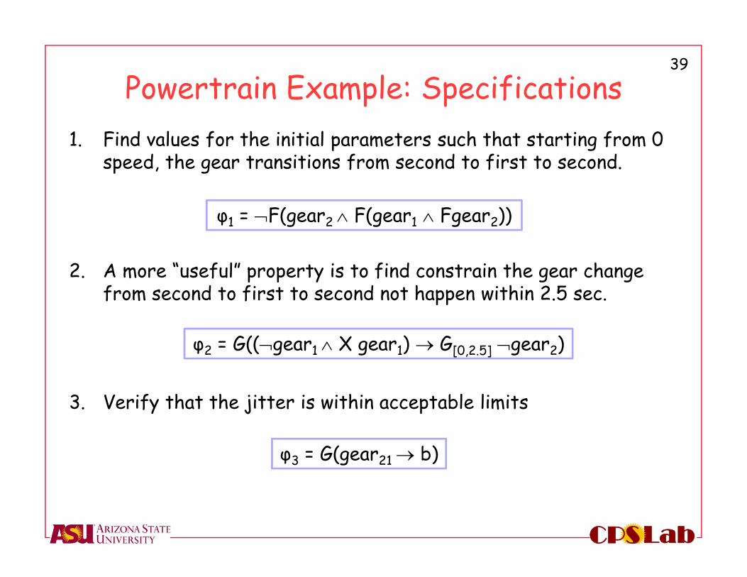
Powertrain Example: Specifications1. Find values for the initial parameters such that starting from 0

speed, the gear transitions from second to first to second.

2. A more “useful” property is to find constrain the gear change from second to first to second not happen within 2.5 sec.

3. Verify that the jitter is within acceptable limits

φ1 = F(gear2 F(gear1 Fgear2))

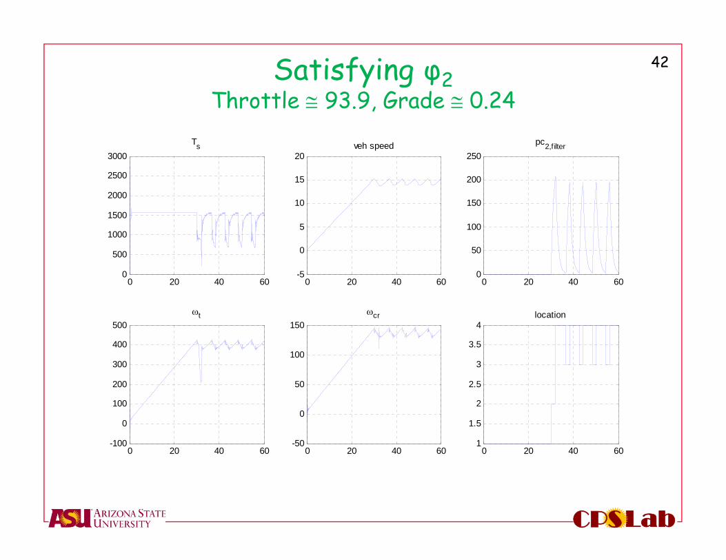
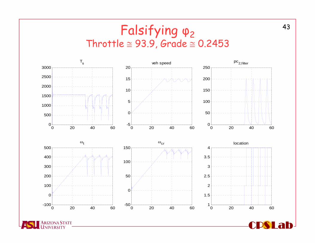
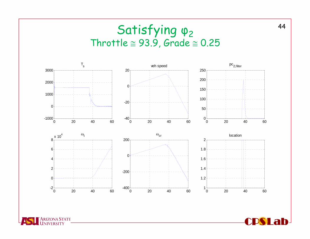
φ2 = G((gear1 X gear1) G[0,2.5] gear2)

φ3 = G(gear21 b)

40

LabCPS

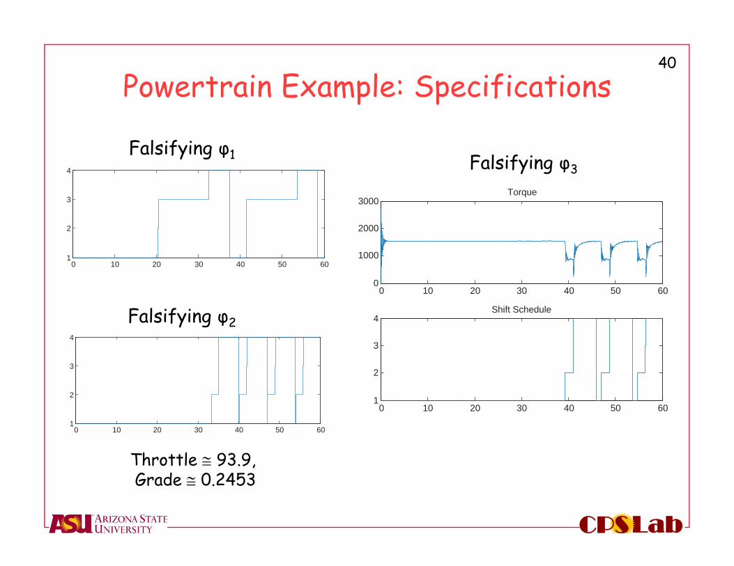
Powertrain Example: Specifications

0 10 20 30 40 50 601

2

3

4

0 10 20 30 40 50 601

2

3

4

0 10 20 30 40 50 600

1000

2000

3000Torque

0 10 20 30 40 50 601

2

3

4Shift Schedule

Falsifying φ1

Falsifying φ2

Falsifying φ3

Throttle 93.9, Grade 0.2453

41

LabCPS

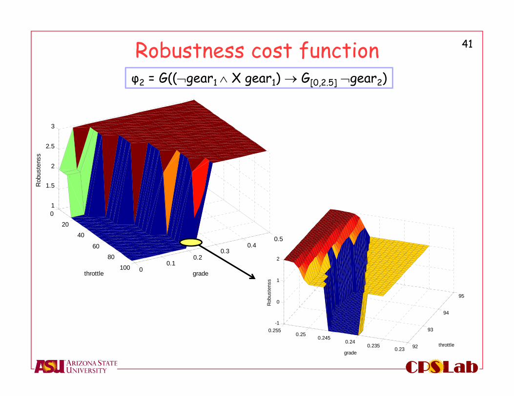
Robustness cost functionφ2 = G((gear1 X gear1) G[0,2.5] gear2)

0

20

40

60

80

100 00.1

0.20.3

0.40.5

1

1.5

2

2.5

3

gradethrottle

Rob

uste

nss

92

93

94

95

0.230.235

0.240.245

0.250.255

-1

0

1

2

throttlegrade

Rob

uste

nss

42

LabCPS

Satisfying φ2Throttle 93.9, Grade 0.24

0 20 40 600

500

1000

1500

2000

2500

3000Ts

0 20 40 60-5

0

5

10

15

20veh speed

0 20 40 600

50

100

150

200

250pc2,filter

0 20 40 60-100

0

100

200

300

400

500t

0 20 40 60-50

0

50

100

150cr

0 20 40 601

1.5

2

2.5

3

3.5

4location

43

LabCPS

Falsifying φ2Throttle 93.9, Grade 0.2453

0 20 40 600

500

1000

1500

2000

2500

3000Ts

0 20 40 60-5

0

5

10

15

20veh speed

0 20 40 600

50

100

150

200

250pc2,filter

0 20 40 60-100

0

100

200

300

400

500t

0 20 40 60-50

0

50

100

150cr

0 20 40 601

1.5

2

2.5

3

3.5

4location

44

LabCPS

Satisfying φ2Throttle 93.9, Grade 0.25

0 20 40 60-1000

0

1000

2000

3000Ts

0 20 40 60-40

-20

0

20veh speed

0 20 40 600

50

100

150

200

250pc2,filter

0 20 40 60-2

0

2

4

6

8x 104 t

0 20 40 60-400

-200

0

200cr

0 20 40 601

1.2

1.4

1.6

1.8

2location

45

LabCPS

Conclusions• Functional verification of arbitrary hybrid systems

remains a challenging problem

• Robustness minimization for functional falsification offers a practical alternative

• Future work:• Study convergence properties• Demonstrate applicability over stochastic hybrid systems

46

LabCPS

AcknowledgementsStudents• Houssam Abbas - PhD (ECEE)• Bardh Hoxha – PhD (CIDSE)• Hengyi Yang – MS (CIDSE)Former Students• Y. Annapureddy - MS (CIDSE) • Che Liu – MS (CIDSE)

Recent collaborators• Aarti Gupta (NEC Labs)• Franjo Ivancic (NEC Labs)• Truong Nghiem (UPenn)• George Pappas (UPenn)• Sriram Sankaranarayanan

(U of Colorado)• Koichi Ueda (Toyota)• Hakan Yazarel (Toyota)

Tools at: https://sites.google.com/a/asu.edu/s-taliro/

Sponsors