Study of LGAD with high timing resolution for ILD

M.KuharaA ,

T. SueharaA, K. KawagoeA , T. YoshiokaB, Y. KatoC

T.OnoeA, S. TsumuraA

(Kyushu Univ.A, RCAPPB, The Univ. of TokyoC)

1

ILD and ECAL

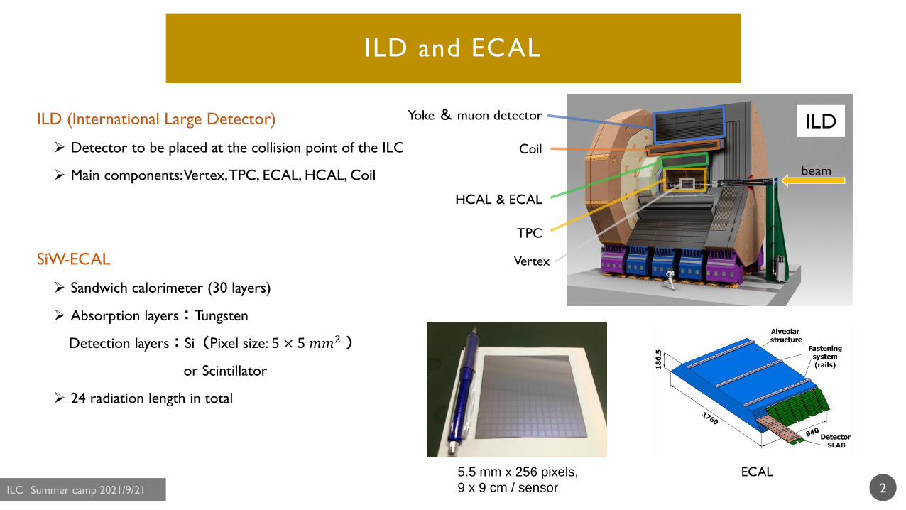
ILD (International Large Detector)

Detector to be placed at the collision point of the ILC

Main components: Vertex, TPC, ECAL, HCAL, Coil

SiW-ECAL

Sandwich calorimeter (30 layers)

Absorption layers：Tungsten

Detection layers：Si（Pixel size: 5 × 5 𝑚𝑚2 ）

or Scintillator

24 radiation length in total

2

ECAL 5.5 mm x 256 pixels,

9 x 9 cm / sensor

Vertex

Particle ID of hadrons and timing resolution

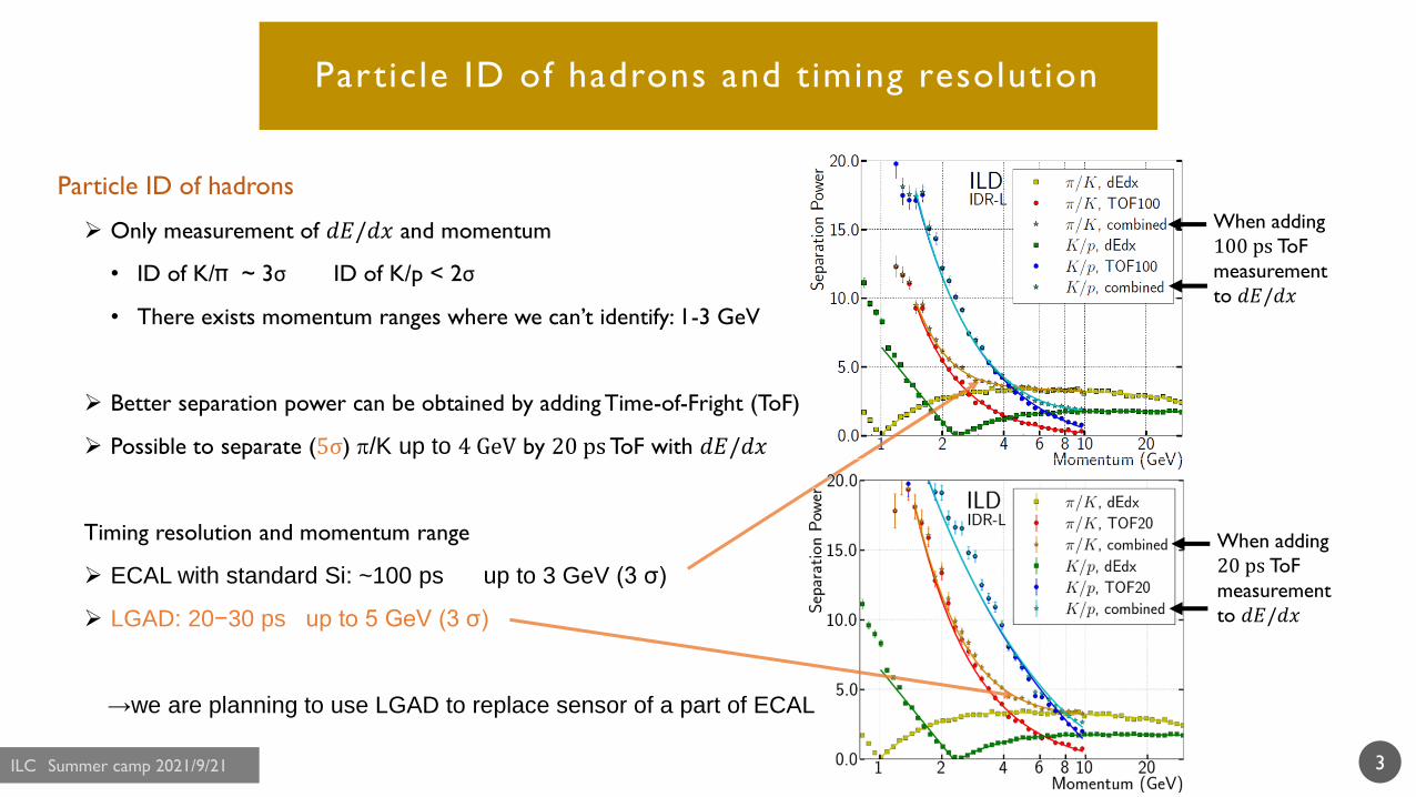
Particle ID of hadrons

Only measurement of 𝑑𝐸/𝑑𝑥 and momentum

• ID of K/π ~ 3σ ID of K/p < 2σ

• There exists momentum ranges where we can’t identify: 1-3 GeV

Better separation power can be obtained by adding Time-of-Fright (ToF)

Possible to separate (5σ) p/K up to 4 GeV by 20 psToF with 𝑑𝐸/𝑑𝑥

Timing resolution and momentum range

ECAL with standard Si: ~100 ps up to 3 GeV (3 σ)

LGAD: 20−30 ps up to 5 GeV (3 σ)

→we are planning to use LGAD to replace sensor of a part of ECAL

3

When adding

100 ps ToF

measurement

to 𝑑𝐸/𝑑𝑥

When adding

20 ps ToF

measurement

to 𝑑𝐸/𝑑𝑥

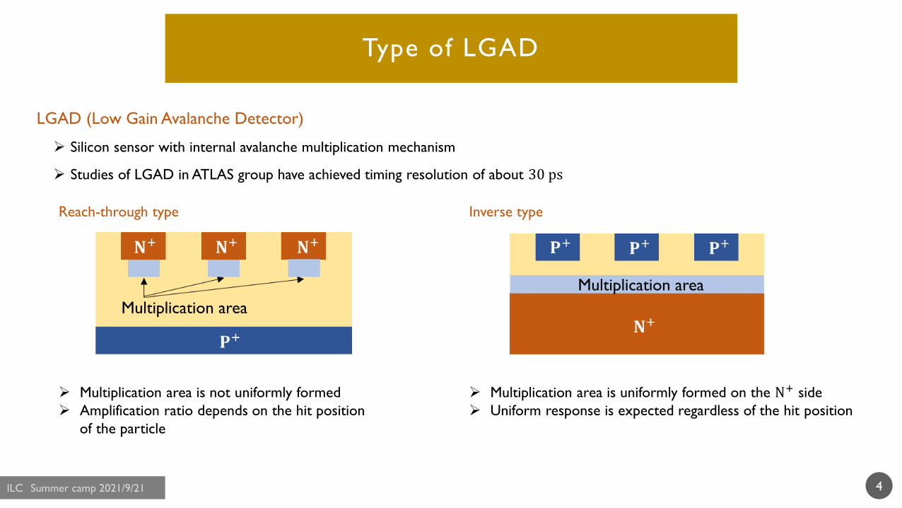
LGAD (Low Gain Avalanche Detector)

Silicon sensor with internal avalanche multiplication mechanism

Studies of LGAD in ATLAS group have achieved timing resolution of about 30 ps

Type of LGAD

4

Reach-through type

Multiplication area is not uniformly formed

Amplification ratio depends on the hit position

of the particle

Inverse type

Multiplication area is uniformly formed on the N+ side

Uniform response is expected regardless of the hit position

Multiplication area

Multiplication area

Test beam

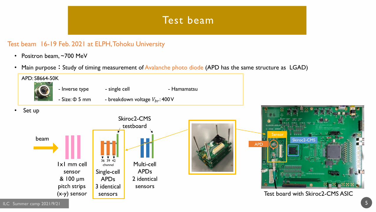
Test beam 16-19 Feb. 2021 at ELPH, Tohoku University

• Positron beam, ~700 MeV

• Main purpose：Study of timing measurement of Avalanche photo diode (APD has the same structure as LGAD)

APD: S8664-50K

- Inverse type - single cell - Hamamatsu

- Size: Φ 5 mm - breakdown voltage 𝑉𝑏𝑟 : 400 V

• Set up

5

Test board with Skiroc2-CMS ASIC

Sensor

APDSkiroc2-CMS

Measurement with Skiroc2-CMS

ASIC for reading signals of silicon sensor

TOA (Time Of Arrival)

Timing information between the triggered

time and the next internal clock

ADC

13 cells waveform digitizer at 50 MHz

ring buffer

6

Pre AMP

Slow shaper

Fast shaper

Result of timing resolution and jitter

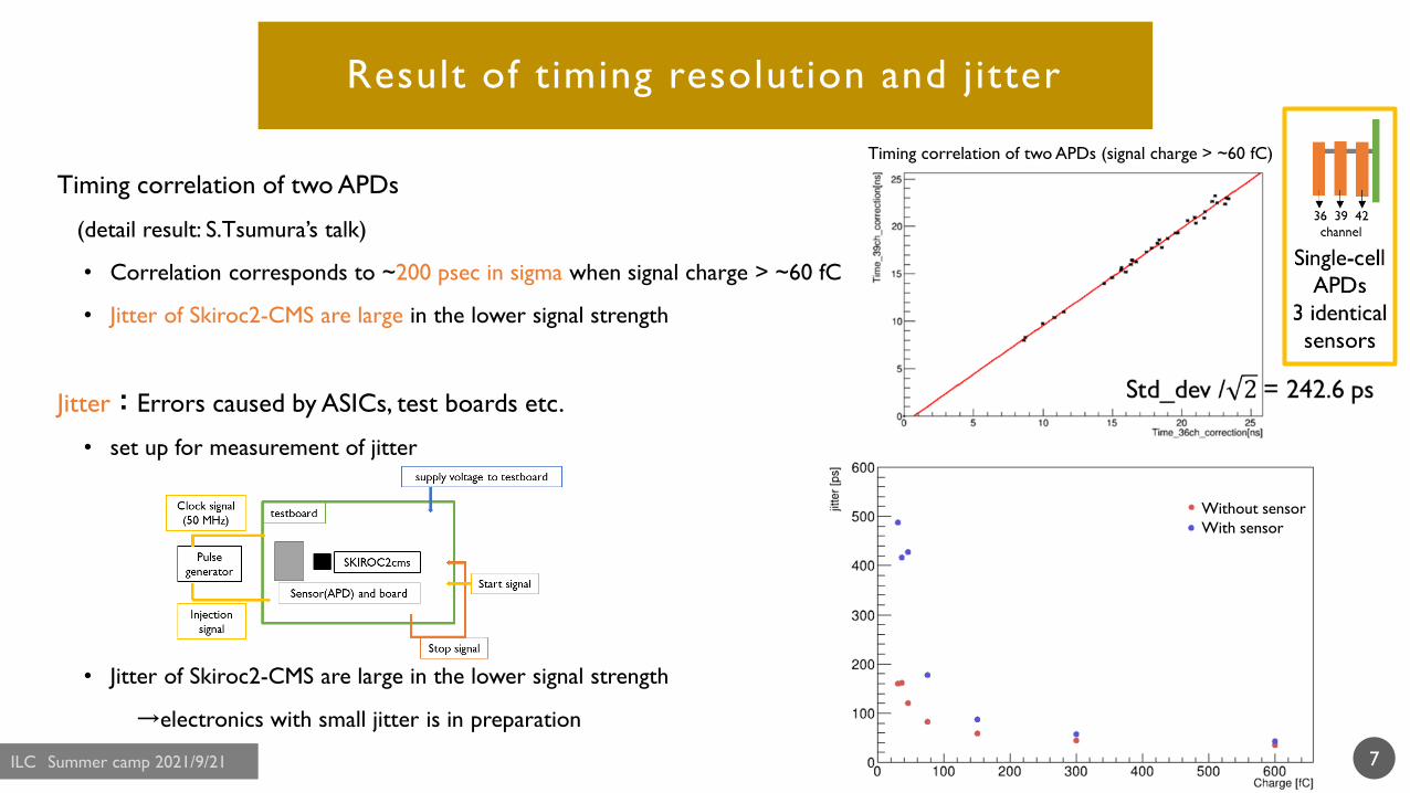
Timing correlation of two APDs

(detail result: S.Tsumura’s talk)

• Correlation corresponds to ~200 psec in sigma when signal charge > ~60 fC

• Jitter of Skiroc2-CMS are large in the lower signal strength

Jitter：Errors caused by ASICs, test boards etc.

• set up for measurement of jitter

• Jitter of Skiroc2-CMS are large in the lower signal strength

→electronics with small jitter is in preparation

7

Without sensor

With sensor

Timing correlation of two APDs (signal charge > ~60 fC)

For achieve high timing resolution

• Timing resolution ≅ (rising time)/(S/N ratio) + digitization jitter + Landau noise + timewalk

noise of Skirock2-CMS is large

rising time of Skiroc2-CMS fast shaper is large: 5 nsec

• Value of S/N ratio ~250 required for 20 ps timing resolution equivalent to 600e- noise too difficult

• Fast shaper can be faster but S/N degraded (need detailed study)

Digitization jitter of Skiroc2-CMS: ~30 ps

Landau noise: waveform changes depending on whether energy deposit occurs

more on the upper side or lower side of the sensor.

Timewalk can be corrected (S.Tsumura’s talk)

• Noise reduction by better HV treatment

• However, to achieve timing resolution 30 ps by noise reduction is difficult… need another reading system

8

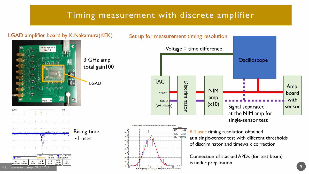
Timing measurement with discrete amplifier

LGAD amplifier board by K.Nakamura(KEK)

3 GHz amp

total gain100

Rising time

~1 nsec

8.4 psec timing resolution obtained

at a single-sensor test with different thresholds

of discriminator and timewalk correction

Connection of stacked APDs (for test beam)

is under preparation 9

Set up for measurement timing resolution

LGAD

Plans at next test beam

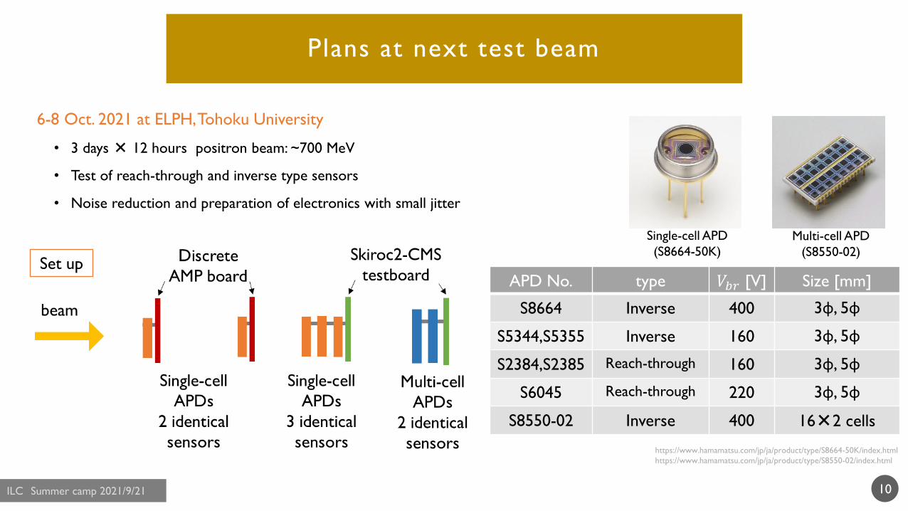
6-8 Oct. 2021 at ELPH, Tohoku University

• 3 days × 12 hours positron beam: ~700 MeV

• Test of reach-through and inverse type sensors

• Noise reduction and preparation of electronics with small jitter

10

APD No. type 𝑉𝑏𝑟 [V] Size [mm]

S8664 Inverse 400 3φ, 5φ

S5344,S5355 Inverse 160 3φ, 5φ

S2384,S2385 Reach-through 160 3φ, 5φ

S6045 Reach-through 220 3φ, 5φ

S8550-02 Inverse 400 16×2 cells

Multi-cell APD

(S8550-02)

https://www.hamamatsu.com/jp/ja/product/type/S8664-50K/index.html

https://www.hamamatsu.com/jp/ja/product/type/S8550-02/index.html

Set up

Single-cell APD

(S8664-50K)

Summary

• LGAD have high timing resolution

• Test beam in February

Obtained timing resolution of inverse type APD (S8664-50K): ~ 200 ps for signal with ~60 fC

Jitter of Skiroc2-CMS are large in the lower signal strength

• Preparation for next test beam

Test of reach-through and inverse type APD sensors

Electronics with small jitter is in preparation

Lowering threshold (noise reduction)

Measurement with discrete amplifier

11

BACKUP

12

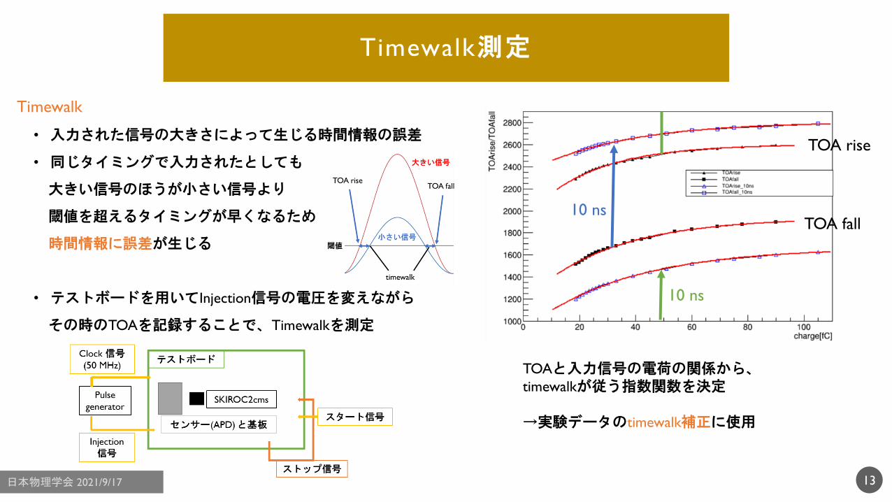
Timewalk測定

Timewalk

• 入力された信号の大きさによって生じる時間情報の誤差

• 同じタイミングで入力されたとしても

大きい信号のほうが小さい信号より

閾値を超えるタイミングが早くなるため

時間情報に誤差が生じる

• テストボードを用いてInjection信号の電圧を変えながら

その時のTOAを記録することで、Timewalkを測定

13

TOAと入力信号の電荷の関係から、timewalkが従う指数関数を決定

→実験データのtimewalk補正に使用

TOA rise

TOA fall10 ns

10 ns

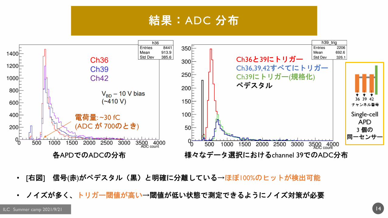
結果：ADC 分布

14

各APDでのADCの分布 様々なデータ選択におけるchannel 39でのADC分布

電荷量: ~30 fC

(ADC が 700のとき)

• [右図] 信号(赤)がペデスタル（黒）と明確に分離している→ほぼ100%のヒットが検出可能

• ノイズが多く、トリガー閾値が高い→閾値が低い状態で測定できるようにノイズ対策が必要

Ch36と39にトリガーCh36,39,42すべてにトリガーCh39にトリガー(規格化)

ペデスタル

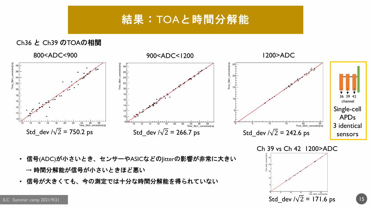
結果：TOAと時間分解能

15

• 信号(ADC)が小さいとき、センサーやASICなどのJitterの影響が非常に大きい

→時間分解能が信号が小さいときほど悪い

• 信号が大きくても、今の測定では十分な時間分解能を得られていない

800<ADC<900 900<ADC<1200 1200>ADC

Ch36 と Ch39 のTOAの相関

Std_dev / 2 = 750.2 ps Std_dev / 2 = 266.7 ps Std_dev / 2 = 242.6 ps

Ch 39 vs Ch 42 1200>ADC

Std_dev / 2 = 171.6 ps

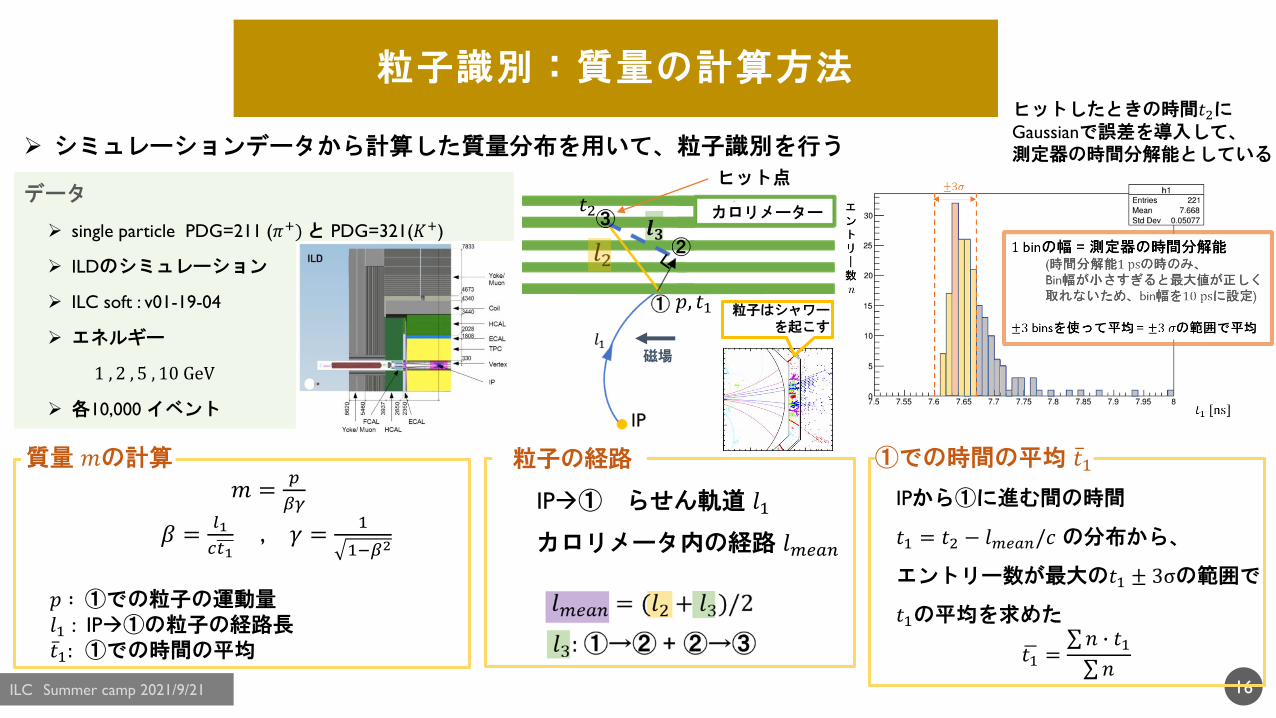
粒子識別：質量の計算方法

16

データ

single particle PDG=211 (𝜋+)と PDG=321(𝐾+)

ILDのシミュレーション

ILC soft : v01-19-04

エネルギー

1 , 2 , 5 , 10 GeV

各10,000 イベント

ヒット点

磁場

カロリメーター

𝑝, 𝑡1

𝑡2

シミュレーションデータから計算した質量分布を用いて、粒子識別を行う

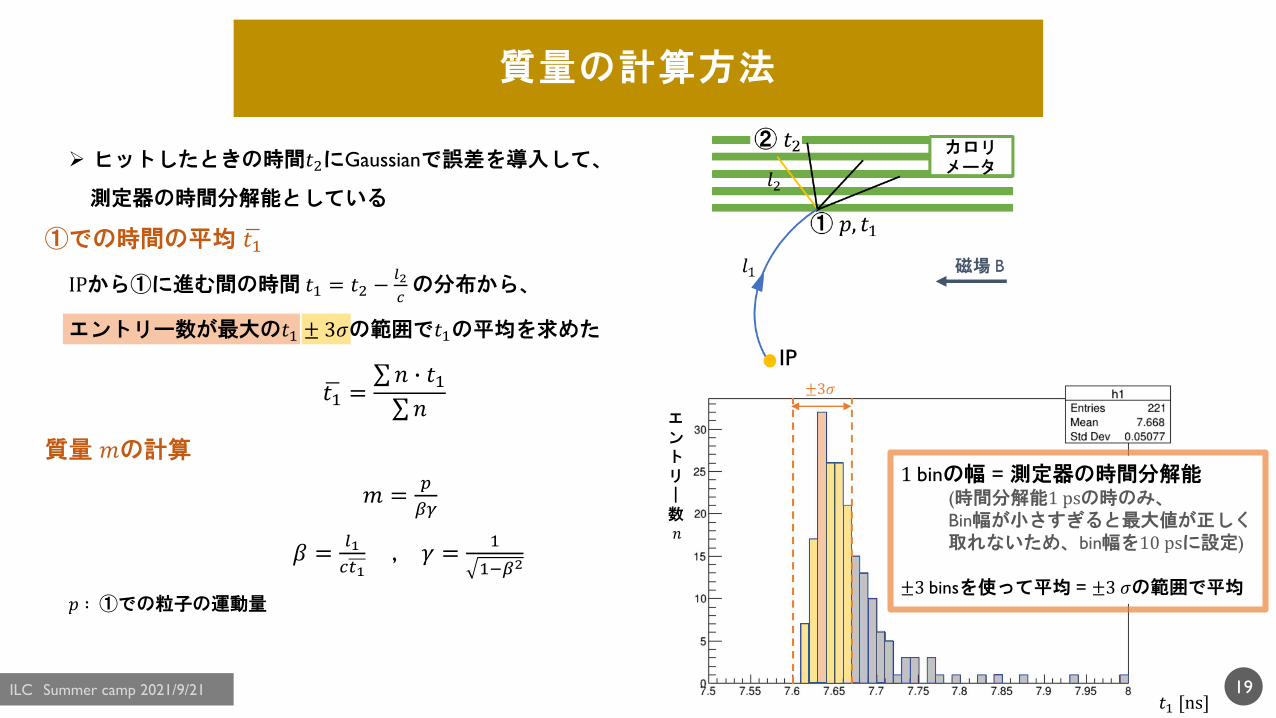
ヒットしたときの時間𝑡2にGaussianで誤差を導入して、測定器の時間分解能としている

質量 𝑚の計算

𝑚 =𝑝

𝛽𝛾

𝛽 =𝑙1

𝑐𝑡1, 𝛾 =

1

1−𝛽2

𝑝 ∶ ①での粒子の運動量𝑙1 : IP①の粒子の経路長ҧ𝑡1: ①での時間の平均

粒子の経路

IP① らせん軌道 𝑙1

カロリメータ内の経路 𝑙𝑚𝑒𝑎𝑛

①での時間の平均 ҧ𝑡1

IPから①に進む間の時間

𝑡1 = 𝑡2 − 𝑙𝑚𝑒𝑎𝑛/𝑐 の分布から、

エントリー数が最大の𝑡1 ± 3σの範囲で

𝑡1の平均を求めた

ഥ𝑡1 =σ𝑛 ∙ 𝑡1σ𝑛

磁場

粒子はシャワーを起こす

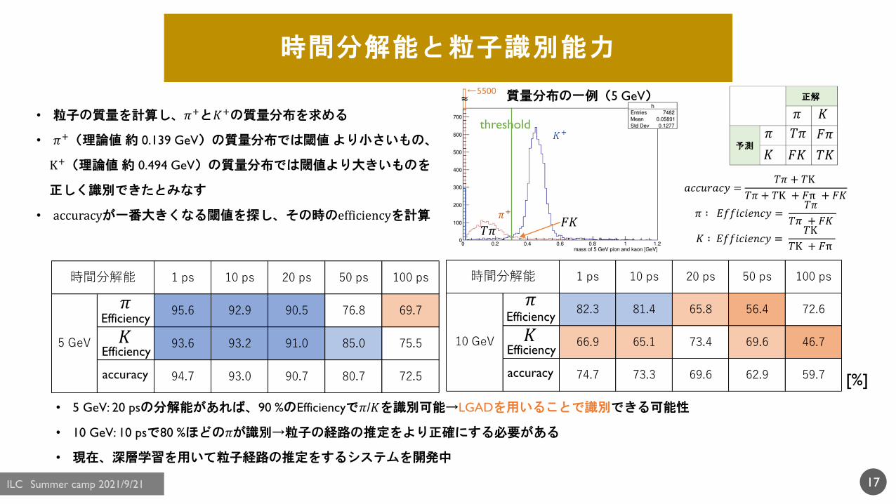
1 ps 10 ps 20 ps 50 ps 100 ps

95.6 92.9 90.5 76.8 69.7

93.6 93.2 91.0 85.0 75.5

94.7 93.0 90.7 80.7 72.5

時間分解能

5 GeV

時間分解能と粒子識別能力

• 粒子の質量を計算し、𝜋+と𝐾+の質量分布を求める

• 𝜋+（理論値約 0.139 GeV）の質量分布では閾値より小さいもの、

K+（理論値約 0.494 GeV）の質量分布では閾値より大きいものを

正しく識別できたとみなす

• accuracyが一番大きくなる閾値を探し、その時のefficiencyを計算

17

𝜋

𝐾Efficiency

Efficiency

accuracy

1 ps 10 ps 20 ps 50 ps 100 ps

82.3 81.4 65.8 56.4 72.6

66.9 65.1 73.4 69.6 46.7

74.7 73.3 69.6 62.9 59.7

時間分解能

10 GeV

𝜋

𝐾Efficiency

Efficiency

accuracy[%]

𝑎𝑐𝑐𝑢𝑟𝑎𝑐𝑦 =𝑇𝜋 + 𝑇K

𝑇𝜋 + 𝑇K + 𝐹π + 𝐹𝐾

𝜋 ∶ 𝐸𝑓𝑓𝑖𝑐𝑖𝑒𝑛𝑐𝑦 =𝑇𝜋

𝑇𝜋 + 𝐹𝐾

𝐾 ∶ 𝐸𝑓𝑓𝑖𝑐𝑖𝑒𝑛𝑐𝑦 =𝑇K

𝑇K + 𝐹π

𝑇𝜋𝐹𝐾

threshold

• 5 GeV: 20 psの分解能があれば、90 %のEfficiencyで𝜋/𝐾を識別可能→LGADを用いることで識別できる可能性

• 10 GeV: 10 psで80 %ほどの𝜋が識別→粒子の経路の推定をより正確にする必要がある

• 現在、深層学習を用いて粒子経路の推定をするシステムを開発中

質量分布の一例（5 GeV）

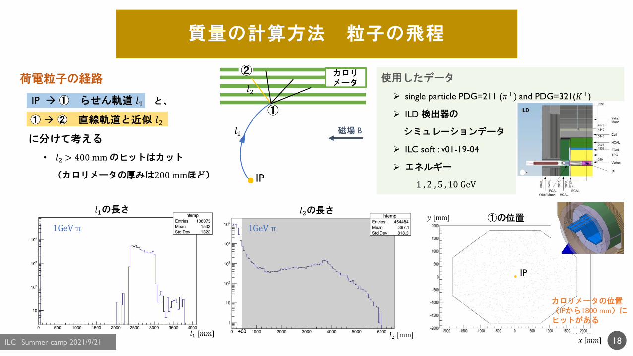
質量の計算方法 粒子の飛程

18

荷電粒子の経路

IP ① らせん軌道 𝑙1 と、

①② 直線軌道と近似 𝑙2

に分けて考える

• 𝑙2 > 400 mmのヒットはカット

（カロリメータの厚みは200 mmほど）

𝑥 [𝑚𝑚]

𝑦 [mm] ①の位置

IP

カロリメータの位置（IPから1800 mm）にヒットがある

𝑙1の長さ

𝑙1 [𝑚𝑚]

𝑙2の長さ

使用したデータ

single particle PDG=211 (𝜋+) and PDG=321(𝐾+)

ILD 検出器の

シミュレーションデータ

ILC soft : v01-19-04

エネルギー

1 , 2 , 5 , 10 GeV

1GeV π 1GeV π

質量の計算方法

19

ヒットしたときの時間𝑡2にGaussianで誤差を導入して、

測定器の時間分解能としている

①での時間の平均 ഥ𝑡1

IPから①に進む間の時間 𝑡1 = 𝑡2 −𝑙2

𝑐の分布から、

エントリー数が最大の𝑡1 ± 3𝜎の範囲で𝑡1の平均を求めた

ഥ𝑡1 =σ𝑛 ∙ 𝑡1σ𝑛

質量 𝑚の計算

𝑚 =𝑝

𝛽𝛾

𝛽 =𝑙1

𝑐𝑡1, 𝛾 =

1

1−𝛽2

𝑝 ∶ ①での粒子の運動量

𝑡1 [ns]

エントリ｜数𝑛

±3𝜎

1 binの幅 = 測定器の時間分解能(時間分解能1 psの時のみ、Bin幅が小さすぎると最大値が正しく取れないため、bin幅を10 psに設定)

±3 binsを使って平均 = ±3 𝜎の範囲で平均

粒子の質量分布

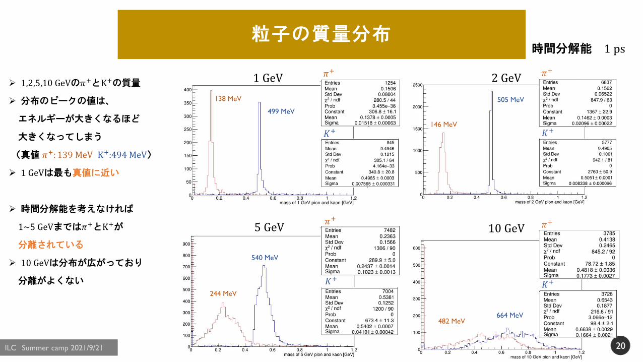
1,2,5,10 GeVの𝜋+とK+の質量

分布のピークの値は、

エネルギーが大きくなるほど

大きくなってしまう

（真値 𝜋+: 139 MeV K+:494 MeV）

1 GeVは最も真値に近い

時間分解能を考えなければ

1~5 GeVまでは𝜋+とK+が

分離されている

10 GeVは分布が広がっており

分離がよくない

20

1 GeV 2 GeV

5 GeV 10 GeV

20

𝜋+

𝐾+

138 MeV

146 MeV

244 MeV

482 MeV

499 MeV

505 MeV

540 MeV

664 MeV

𝜋+

𝐾+

𝜋+

𝐾+

𝜋+

𝐾+

時間分解能 1 ps

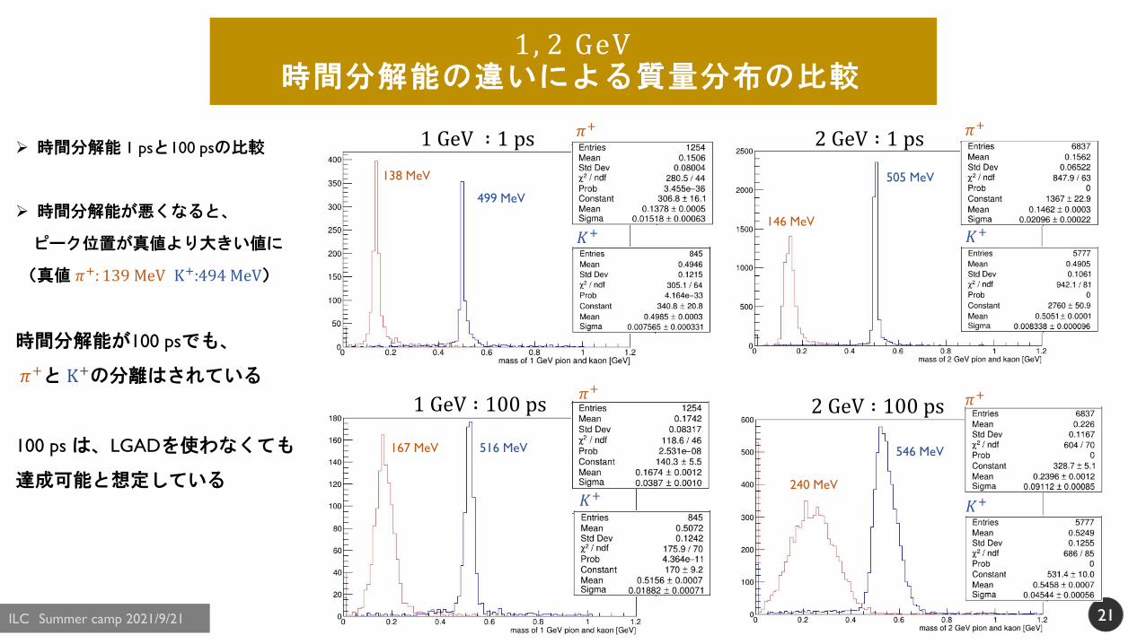
1, 2 GeV時間分解能の違いによる質量分布の比較

時間分解能 1 psと100 psの比較

時間分解能が悪くなると、

ピーク位置が真値より大きい値に

（真値 𝜋+: 139 MeV K+:494 MeV）

時間分解能が100 psでも、

𝜋+と K+の分離はされている

100 psは、LGADを使わなくても

達成可能と想定している

21

1 GeV ∶ 1 ps 2 GeV ∶ 1 ps

1 GeV ∶ 100 ps 2 GeV ∶ 100 ps

21

𝜋+

𝐾+

138 MeV

146 MeV

167 MeV

240 MeV

499 MeV

505 MeV

516 MeV 546 MeV

𝜋+

𝐾+

𝜋+

𝐾+

𝜋+

𝐾+

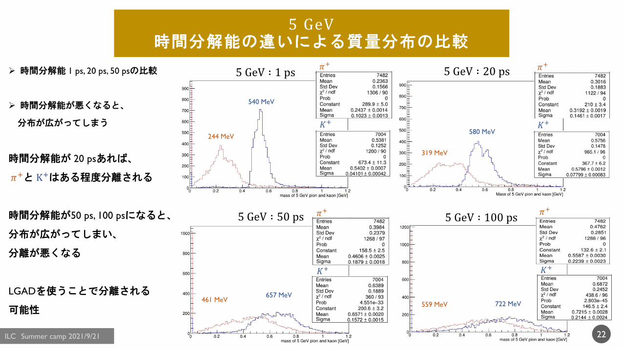
5 GeV時間分解能の違いによる質量分布の比較

5 GeV ∶ 20 ps

5 GeV ∶ 50 ps

5 GeV ∶ 1 ps𝜋+

𝐾+

319 MeV

461 MeV

244 MeV580 MeV

657 MeV

540 MeV

𝜋+

𝐾+

𝜋+

𝐾+

時間分解能 1 ps, 20 ps, 50 psの比較

時間分解能が悪くなると、

分布が広がってしまう

時間分解能が 20 psあれば、

𝜋+と K+はある程度分離される

時間分解能が50 ps, 100 psになると、

分布が広がってしまい、

分離が悪くなる

LGADを使うことで分離される

可能性

22

5 GeV ∶ 100 ps𝜋+

𝐾+

559 MeV 722 MeV

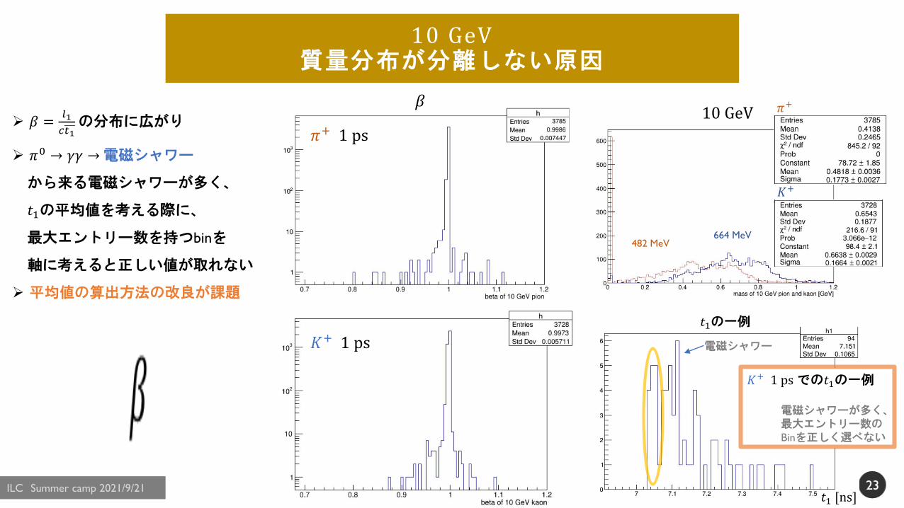
10 GeV質量分布が分離しない原因

2323

𝛽 =𝑙1

𝑐𝑡1の分布に広がり

𝜋0 → 𝛾𝛾 →電磁シャワー

から来る電磁シャワーが多く、

𝑡1の平均値を考える際に、

最大エントリー数を持つbinを

軸に考えると正しい値が取れない

平均値の算出方法の改良が課題

10 GeV

482 MeV664 MeV

𝜋+

𝐾+

𝜋+ 1 ps

𝛽

𝐾+ 1 ps

𝑡1 [ns]

𝐾+ 1 psでの𝑡1の一例

電磁シャワーが多く、最大エントリー数のBinを正しく選べない

𝑡1の一例

電磁シャワー

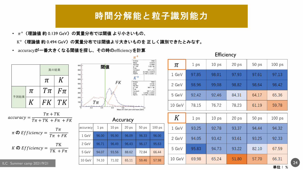
時間分解能と粒子識別能力

• 𝜋+（理論値約 0.139 GeV）の質量分布では閾値より小さいもの、

K+（理論値約 0.494 GeV）の質量分布では閾値より大きいものを正しく識別できたとみなす。

• accuracyが一番大きくなる閾値を探し、その時のefficiencyを計算

24単位： %

Efficiency

𝜋

𝐾

𝜋

𝜋

𝐾

𝐾

𝑇𝜋 𝐹𝜋

𝐹𝐾 𝑇𝐾

𝜋+

𝐾+

𝑇𝜋

𝐹𝐾

閾値

𝑎𝑐𝑐𝑢𝑟𝑎𝑐𝑦 =𝑇𝜋 + 𝑇K

𝑇𝜋 + 𝑇K + 𝐹π + 𝐹𝐾

𝜋の 𝐸𝑓𝑓𝑖𝑐𝑖𝑒𝑛𝑐𝑦 =𝑇𝜋

𝑇𝜋 + 𝐹𝐾

𝐾の 𝐸𝑓𝑓𝑖𝑐𝑖𝑒𝑛𝑐𝑦 =𝑇K

𝑇K + 𝐹π

真の結果

予測結果

accuracy 1 ps 10 ps 20 ps 50 ps 100 ps

1 GeV 96.00 95.90 96.09 96.33 96.00

2 GeV 96.71 96.49 96.43 96.17 95.63

5 GeV 94.07 93.56 88.62 72.84 66.44

10 GeV 74.10 71.02 65.11 59.46 57.98

Accuracy

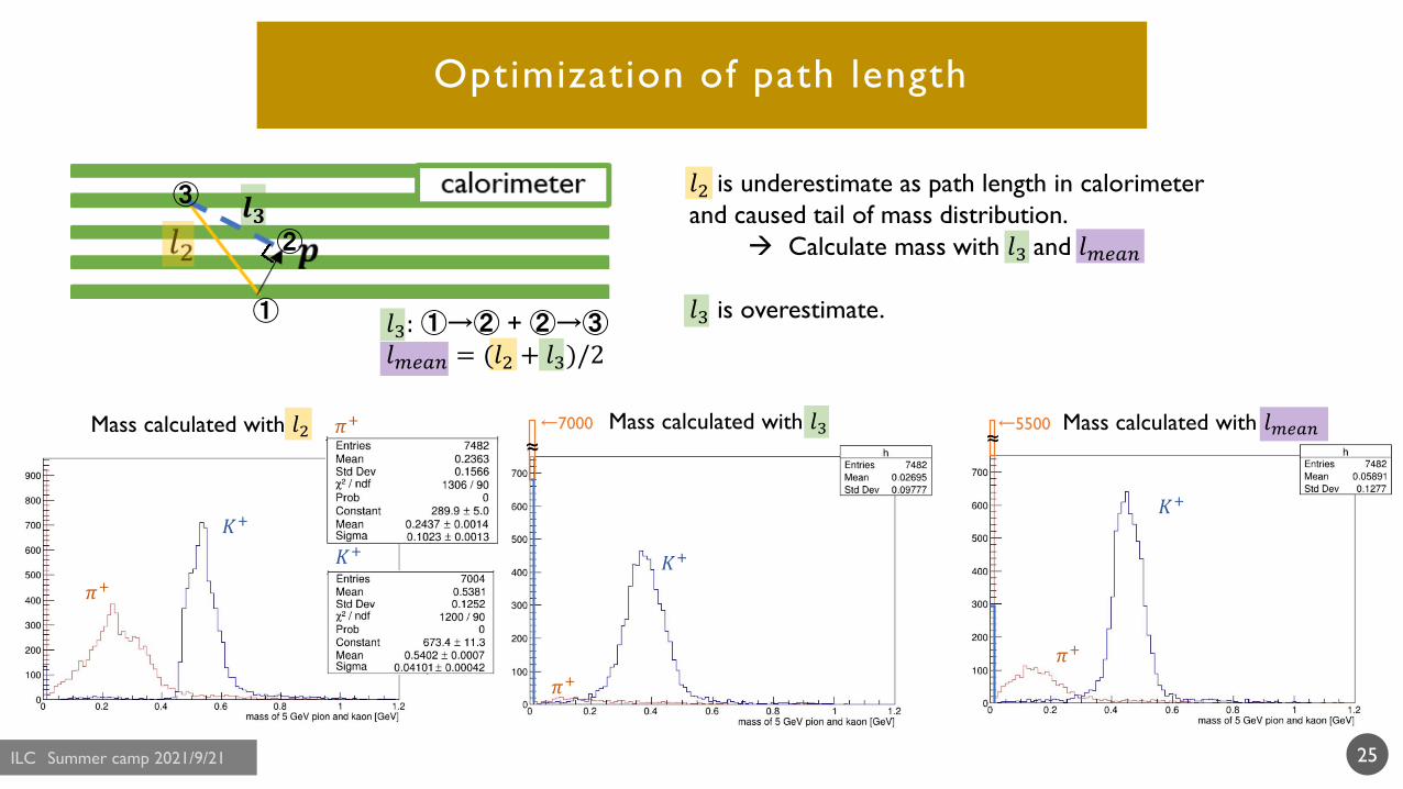
Optimization of path length

25

𝜋+

𝐾+

𝒍𝟑

①

②

③

𝑙3:①→② + ②→③𝑙𝑚𝑒𝑎𝑛 = (𝑙2 + 𝑙3)/2

Mass calculated with 𝑙3 Mass calculated with 𝑙𝑚𝑒𝑎𝑛

𝜋+

𝐾+

𝜋+

𝐾+

←7000 ←5500Mass calculated with 𝑙2

𝜋+

𝐾+

𝑙2 is underestimate as path length in calorimeter

and caused tail of mass distribution.

Calculate mass with 𝑙3 and 𝑙𝑚𝑒𝑎𝑛

𝑙3 is overestimate.

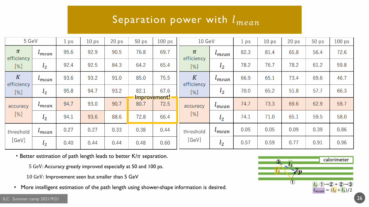
Separation power with 𝑙𝑚𝑒𝑎𝑛

・Better estimation of path length leads to better K/𝜋 separation.

5 GeV:Accuracy greatly improved especially at 50 and 100 ps.

10 GeV: Improvement seen but smaller than 5 GeV

• More intelligent estimation of the path length using shower-shape information is desired.

26

Improvement!

Layers with different time resolution

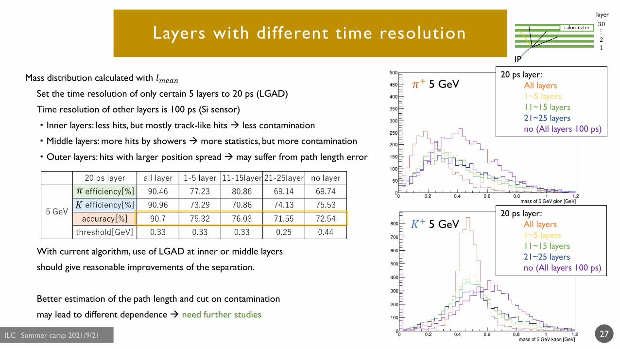
Mass distribution calculated with 𝑙𝑚𝑒𝑎𝑛

Set the time resolution of only certain 5 layers to 20 ps (LGAD)

Time resolution of other layers is 100 ps (Si sensor)

・Inner layers: less hits, but mostly track-like hits less contamination

・Middle layers: more hits by showers more statistics, but more contamination

・Outer layers: hits with larger position spread may suffer from path length error

With current algorithm, use of LGAD at inner or middle layers

should give reasonable improvements of the separation.

Better estimation of the path length and cut on contamination

may lead to different dependence need further studies

27

𝜋+ 5 GeV

𝐾+ 5 GeV

20 ps layer all layer 1-5 layer 11-15layer 21-25layer no layer

efficiency[%] 90.46 77.23 80.86 69.14 69.74

efficiency[%] 90.96 73.29 70.86 74.13 75.53

accuracy[%] 90.7 75.32 76.03 71.55 72.54

threshold[GeV] 0.33 0.33 0.33 0.25 0.44

5 GeV

𝜋

𝐾

20 ps layer:

All layers

1~5 layers

11~15 layers

21~25 layers

no (All layers 100 ps)

20 ps layer:

All layers

1~5 layers

11~15 layers

21~25 layers

no (All layers 100 ps)

IP

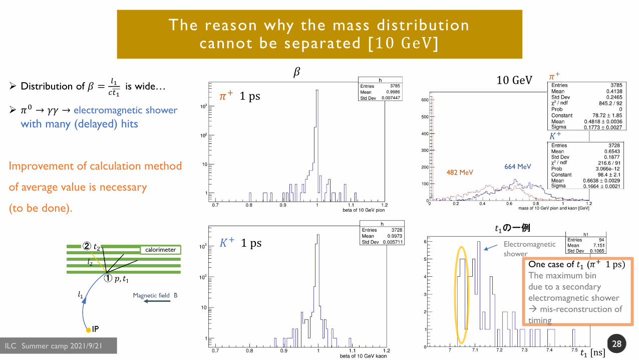
The reason why the mass distribution cannot be separated [10 GeV]

2828

Distribution of 𝛽 =𝑙1

𝑐𝑡1is wide…

𝜋0 → 𝛾𝛾 → electromagnetic shower

with many (delayed) hits

Improvement of calculation method

of average value is necessary

(to be done).

10 GeV

482 MeV664 MeV

𝜋+

𝐾+

𝜋+ 1 ps

𝛽

𝐾+ 1 ps

𝑡1 [ns]

𝑡1の一例

Electromagnetic

shower

One case of 𝑡1 (𝜋+ 1 ps)The maximum bin

due to a secondary

electromagnetic shower

mis-reconstruction of

timing

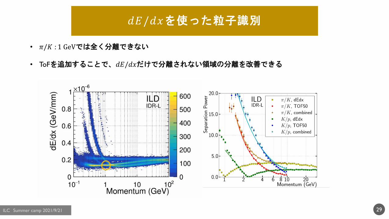
𝑑𝐸/𝑑𝑥を使った粒子識別

29

• 𝜋/𝐾 : 1 GeVでは全く分離できない

• ToFを追加することで、𝑑𝐸/𝑑𝑥だけで分離されない領域の分離を改善できる

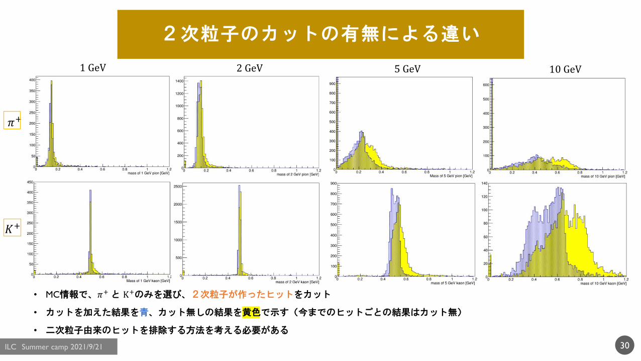
２次粒子のカットの有無による違い

• MC情報で、𝜋+と K+のみを選び、２次粒子が作ったヒットをカット

• カットを加えた結果を青、カット無しの結果を黄色で示す（今までのヒットごとの結果はカット無）

• 二次粒子由来のヒットを排除する方法を考える必要がある

30

𝜋+

𝐾+

1 GeV 2 GeV 5 GeV 10 GeV

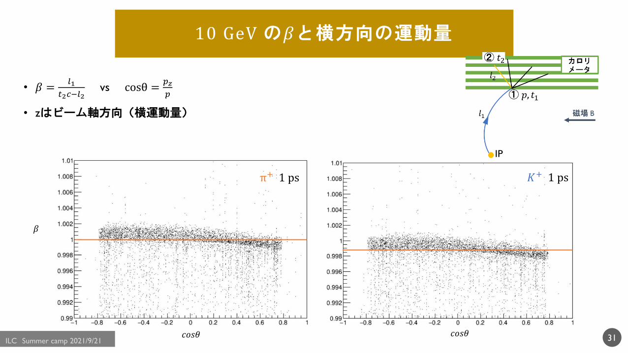
10 GeV の𝛽と横方向の運動量

• 𝛽 =𝑙1

𝑡2𝑐−𝑙2vs cosθ =

𝑝𝑧

𝑝

• zはビーム軸方向（横運動量）

31

𝐾+ 1 psπ+ 1 ps

𝛽

𝑐𝑜𝑠𝜃 𝑐𝑜𝑠𝜃

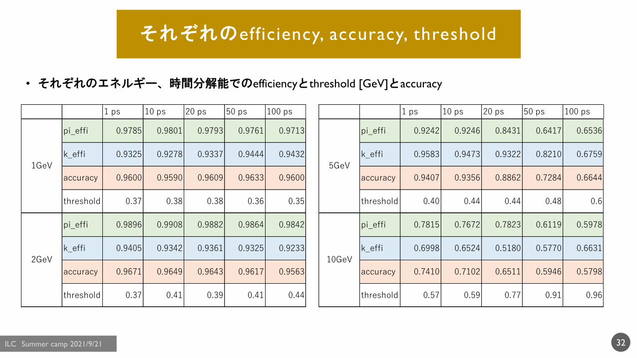
それぞれのefficiency, accuracy, threshold

• それぞれのエネルギー、時間分解能でのefficiencyとthreshold [GeV]とaccuracy

32

1 ps 10 ps 20 ps 50 ps 100 ps

pi_effi 0.9785 0.9801 0.9793 0.9761 0.9713

k_effi 0.9325 0.9278 0.9337 0.9444 0.9432

accuracy 0.9600 0.9590 0.9609 0.9633 0.9600

threshold 0.37 0.38 0.38 0.36 0.35

pi_effi 0.9896 0.9908 0.9882 0.9864 0.9842

k_effi 0.9405 0.9342 0.9361 0.9325 0.9233

accuracy 0.9671 0.9649 0.9643 0.9617 0.9563

threshold 0.37 0.41 0.39 0.41 0.44

1GeV

2GeV

1 ps 10 ps 20 ps 50 ps 100 ps

pi_effi 0.9242 0.9246 0.8431 0.6417 0.6536

k_effi 0.9583 0.9473 0.9322 0.8210 0.6759

accuracy 0.9407 0.9356 0.8862 0.7284 0.6644

threshold 0.40 0.44 0.44 0.48 0.6

pi_effi 0.7815 0.7672 0.7823 0.6119 0.5978

k_effi 0.6998 0.6524 0.5180 0.5770 0.6631

accuracy 0.7410 0.7102 0.6511 0.5946 0.5798

threshold 0.57 0.59 0.77 0.91 0.96

5GeV

10GeV