Steven J. Cox and Antoine Henrot...Steven J. Cox1 and Antoine Henrot2 Abstract. One may produce the...

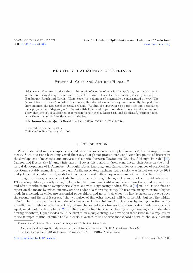
ESAIM: COCV 14 (2008) 657–677 ESAIM: Control, Optimisation and Calculus of Variations

DOI: 10.1051/cocv:2008004 www.esaim-cocv.org

ELICITING HARMONICS ON STRINGS

Steven J. Cox1 and Antoine Henrot2

Abstract. One may produce the qth harmonic of a string of length π by applying the ‘correct touch’at the node π/q during a simultaneous pluck or bow. This notion was made precise by a model ofBamberger, Rauch and Taylor. Their ‘touch’ is a damper of magnitude b concentrated at π/q. The‘correct touch’ is that b for which the modes, that do not vanish at π/q, are maximally damped. Wehere examine the associated spectral problem. We find the spectrum to be periodic and determinedby a polynomial of degree q − 1. We establish lower and upper bounds on the spectral abscissa andshow that the set of associated root vectors constitutes a Riesz basis and so identify ‘correct touch’with the b that minimizes the spectral abscissa.

Mathematics Subject Classification. 35P10, 35P15, 74K05, 74P10.

Received September 5, 2006.Published online January 18, 2008.

1. Introduction

We are interested in one’s capacity to elicit harmonic overtones, or simply ‘harmonics’, from stringed instru-ments. Such questions have long vexed theorists, though not practitioners, and were key points of friction inthe development of mechanics and analysis in the period between Newton and Cauchy. Although Truesdell [30],Cannon and Dostrovsky [6] and Christensen [7] cover this period in fascinating detail, their focus on the intel-lectual developments of D’Alembert, Bernoulli, Euler, Lagrange and Rameau, leaves a number of practical in-novations, notably harmonics, in the dark. As the associated mathematical question was in fact well set by 1692and yet its mathematical analysis did not commence until 1982 we open with an outline of the full history.

Though overtones, or upper partials, had been heard through the ages they were not seen until late in the17th century. More precisely, though Descartes, Mersenne and Galileo each remark on the sound of overtonesand often ascribe them to sympathetic vibrations with neighboring bodies, Wallis [32] in 1677 is the first toreport on the means by which one may see the nodes of a vibrating string. He uses one string to excite a highermode in a second, on which are suspended paper riders, and notes that, when the first is tuned an octave abovethe second, and the first is struck, “the two halves of this other [second] will both tremble; but not the middlepoint”. He proceeds to find the nodes of what we call the third and fourth modes by tuning the first stringa twelfth and double octave, respectively, above the second and observes that these nodes divide the string inequal, or aliquot, parts. Roberts [27] in 1692 was the first to observe that, by softly pressing at a node whilebowing elsewhere, higher modes could be elicited on a single string. He developed these ideas in his explicationof the trumpet marine, or nun’s fiddle, a curious variant of the ancient monochord on which the only pleasant

Keywords and phrases. Point-wise damping, spectral abscissa, Riesz basis.

1 Computational and Applied Mathematics, Rice University, Houston, TX, USA; [email protected] Institut Elie Cartan, UMR 7502, Nancy Universite - CNRS - INRIA, Nancy, France.

Article published by EDP Sciences c© EDP Sciences, SMAI 2008

http://dx.doi.org/10.1051/cocv:2008004

http://www.esaim-cocv.org

http://www.edpsciences.org

658 S.J. COX AND A. HENROT

tones are harmonics. Roberts writes “Now in the Trumpet-Marine you do not stop close as in other instruments,but touch the String gently with your thumb, whereby there is mutual concurrence of the upper and lower partof the String to produce the sound” and observes “that the Trumpet Marine will yield no musical sound butwhen the stop makes the upper part of the string an aliquot of the remainder, and consequently of the whole”.Roberts concludes with a lovely figure that includes both a clear indication of the first three theoretical modeshapes and a practical diagram of the 15 nodes at which the player ought to gently thumb.

After Roberts the theory and practice of harmonics regrettably diverge over the course of the 18th century.On the practical side we have Mondonville’s opus 4, Les Sons Harmoniques [3], of 1735, the first pieces scoredfor violin harmonics, complete with a beautiful diagram identifying notes with nodes. On the theoretical side,the mode shapes of Roberts were not to reappear until the 1747 study by Bernoulli [4], a work that stemmed notfrom Roberts’ practical considerations but from the theoretical work of Taylor [29]. In struggling to understandhow a single string could simultaneously support so many modes, Bernoulli, Euler and Lagrange, see [6,23,26],brought forth trigonometric series but rejected these in favor of Euler and D’Alembert’s general wave solutionand vague reference to sympathetic resonance. None of these four men were aware of the simple mechanicalmeans, of Roberts and Mondonville, for eliciting these individual modes. This is remarkable given the presenceof Rameau, a composer and music theorist, hailed as the ‘Newton of Harmony’, (see [6], p. 8), who not onlyentered into substantive individual correspondence with Bernoulli, Euler, Lagrange and D’Alembert but whowas also surely aware of both the strange flageolet tones of the trumpet marine and the works of Mondonville.Regarding Rameau’s influence on Bernoulli et al. see Truesdell [30] and especially Christensen [7]. Galpin [12]informs us that Rameau’s tenure with the orchestra of the Academie du Concert of Lyon overlapped withthat of Prin, the established master of the trumpet marine. Rameau, in the preface to his Pieces de Clavecinen concert, 1741, speaks of the recent success of such ensemble pieces (most likely Mondonville’s opus 5, seeGirdlestone [13], p. 43) and names one of his own pieces after Boucon, his student and the wife of Mondonville.And yet, although Rameau [25], p. 8, was aware of the work of Sauveur [28] on overtones, or “petits sons”,neither Prin’s nor Mondonville’s harmonics figure anywhere in Rameau’s vast theoretical writings. Rameau’sfailure to recognize the theoretical importance of their work contributed to a neglect, over the ensuing 100years, of the study of harmonics. This is, unfortunately, in accord with Miller’s dark verdict, [24], p. 37, that“A careful search fails to reveal any major contribution to the science of sound which arose in the 18th century”.

It is not until 1807 in the work of Young [35], lect. 32, that we find a lucid synthesis of Roberts andMondonville: “if a long chord be initially divided into any number of such equal portions, its parts will continueto vibrate in the same manner as if they were separate chords; the points of division only remaining always atrest. Such subordinate sounds are called harmonics: they are often produced in violins by lightly touching one ofthe points of division with the finger, when the bow is applied, and in all such cases it may be shown, by puttingsmall feathers or pieces of paper on the string, that the remaining points of division are also quiescent, whilethe intervening points are in motion”. Although Young’s observations were echoed by Helmholtz, 1862, [15],Chapter 4 and illustrated by Tyndall, 1875, [31], Section 3.6, it appears that Rayleigh, 1877, [26], Section 134,in noting that “when but a single point of the string is retarded by friction there are no normal co-ordinatesproperly so called”, was the first to have attempted a mathematical analysis of harmonics. After Rayleighthe problem remained untouched until the beautiful, but little known, 1982 work of Bamberger, Rauch andTaylor [2]. (Coincidentally, the problem of pointwise damping of suspension bridge cables was also first broachedby Kovacs [18] in 1982.)

Bamberger et al. followed Rayleigh in retarding by friction, b, at but a single point, a, the motion of a fixedstring of length π with transverse displacement u. More precisely, they considered

utt − uxx + bδ(x− a)ut = 0, u(0, t) = u(π, t) = 0,

with initial data in the energy space X = H10 (0, π) × L2(0, π) endowed with the inner product

〈[f, g], [u, v]〉 =∫ π

0

{f ′u′ + gv} dx. (1.1)

ELICITING HARMONICS ON STRINGS 659

They showed that if the damping is applied at a rational multiple of π then it only damps those modes notvanishing there. They then equated “correct touch” with the value of b that best damps these remainingmodes. In the case a = π/2 they showed that b = 2 was the correct touch. We here attack the general case byinvestigating the spectra of the associated wave operator

A(a, b) =(

0 I∂xx 0

), x �= a

D(A(a, b)) = {[f, g] ∈ (H10 (0, π) ∩H2(0, a) ∩H2(a, π)) ×H1

0 (0, π) : f ′(a+) − f ′(a−) = bg(a)}.

Bamberger et al. argue that A(a, b) has a compact resolvent and so discrete spectrum and that when a = pπ/q,where p and q are relatively prime integers, it has the imaginary eigenvalues

λ1,n = inq, n ∈ Z \ 0

and associated eigenvectorsV1,n = sin(nqx)[1/(nq) i]. (1.2)

We write σ(pπ/q, b) for the spectrum of A(pπ/q, b) and

σH(pπ/q, b) = {λ1,n} (1.3)

for the harmonic part of the spectrum. It is shown in [2] that the nonharmonic spectrum, σ(pπ/q, b)\σH(pπ/q, b)lies in the strict left half plane and that the semigroup etA(pπ/q,b) enjoys exponential decay on the orthogonalcomplement of the harmonic subspace

H ≡ span{V1,n}.More precisely, denoting the orthogonal complement of H by H⊥, Bamberger et al. establish the existence ofpositive constants, C1 and C2, depending only on p/q and b, such that

‖etA(pπ/q,b)U‖X ≤ C1e−C2t‖U‖X ∀ U ∈ H⊥, t ≥ 0. (1.4)

In this work we shall show the greatest C2 for which (1.4) holds is the magnitude of the nonharmonic spectralabscissa of A(pπ/q, b),

μ(pπ/q, b) ≡ max{�λ : λ ∈ σ(pπ/q, b) \ σH(pπ/q, b)} (1.5)and, along the way, establish bounds on b → μ(a, b) and produce explicit minimizers when a = π/3 anda = π/4. More precisely, in Section 2 we delineate the structure of the spectrum, taking care to identifymultiple eigenvalues and to specify the behavior of the spectrum for b near 0, 2 and ∞. In Section 3 weestablish upper and lower bounds on the nonharmonic spectral abscissa and arrive at the correct touch fora = π/3 and a = π/4. In Section 4 we prove that the associated root vectors comprise a Riesz basis and soidentify μ with the best rate of decay. We close in Section 5 with a return to dimensions and a discussion ofthe true magnitude of b and the role played by an additional elastic term at a.

There exist many works, e.g., Cox and Zuazua [9,10], devoted to the optimal damping of strings, and a sizablemathematical literature, e.g., Liu [22], Jaffard et al. [16], and Ammari et al. [1], and engineering literature, e.g.,Kovacs [18] and Krenk [21], that in fact focus on pointwise damping. As the focus of these previous efforts wason the optimal damping of either all modes or a single mode, the harmonics problem of Bamberger et al. wasnaturally neglected.

2. On the disposition of the spectrum

If A(a, b)[y z] = λ[y z] then z = λy and y must satisfy the quadratic eigenvalue problem

y′′(x) − λ2y(x) − λbδ(x− a)y(x) = 0, y(0) = y(π) = 0.


It is not difficult to show that

y(x) =

{sinh(λ(π − a)) sinh(λx) if 0 < x < a

sinh(λa) sinh(λ(π − x)) if a < x < π

and λ is a zero of the shooting function

S(λ; a, b) = sinh(λπ) + b sinh(λa) sinh(λ(π − a)). (2.1)

The majority of our results are consequences of the simple observation that

S(λ; pπ/q, b) = −(1/4) exp(λπ)P (exp(−2λπ/q); b) (2.2)

where P is the polynomialP (w; b) = (2 − b)wq + bwp + bwq−p − (2 + b). (2.3)

In terms of its roots, {wk = |wk| exp(iθk)}qk=1 (repeated according to their multiplicity), the eigenvalues of

A(a, b) are simply

λk,n =−q2π

{ln |wk| + i(θk + 2πn)}, k = 1, . . . , q, n ∈ Z. (2.4)

For example, if p/q = 1/2 we find P (w; b) = (2− b)w2 + 2bw− 2− b. Its roots, w1 = 1 and w2 = (b+ 2)/(b− 2)translate readily into the associated eigenvalues

λ1,n = i2n, n �= 0

λ2,n = − 1π

ln∣∣∣∣b+ 2b− 2

∣∣∣∣− i(H(2 − b) + 2n)

where H is the Heaviside function. It follows that

μ(π/2, b) = − 1π

ln∣∣∣∣b+ 2b− 2

∣∣∣∣approaches −∞ as b→ 2, in agreement with Bamberger et al.

In preparation for the general case we now examine numerical approximation of the spectra for 0 < b < ∞and q up to 8. Our calculations are facilitated by the fact that the spectrum is completely determined by thepolynomial (2.3) and the observation that

S(λ; a, b) = S(λ; a, b) and S(λ+ qi, pπ/q, b) = (−1)qS(λ, pπ/q, b),

from which we conclude that the spectrum has period qi and that within a period the spectrum is symmetricabout iq/2.

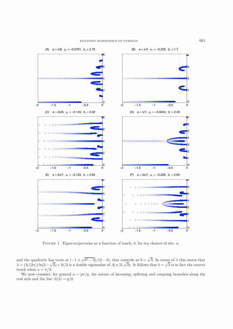
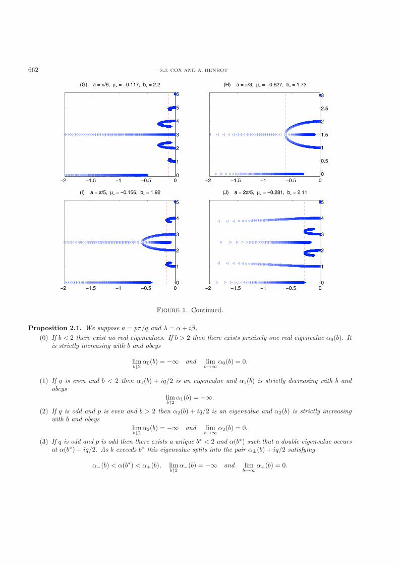
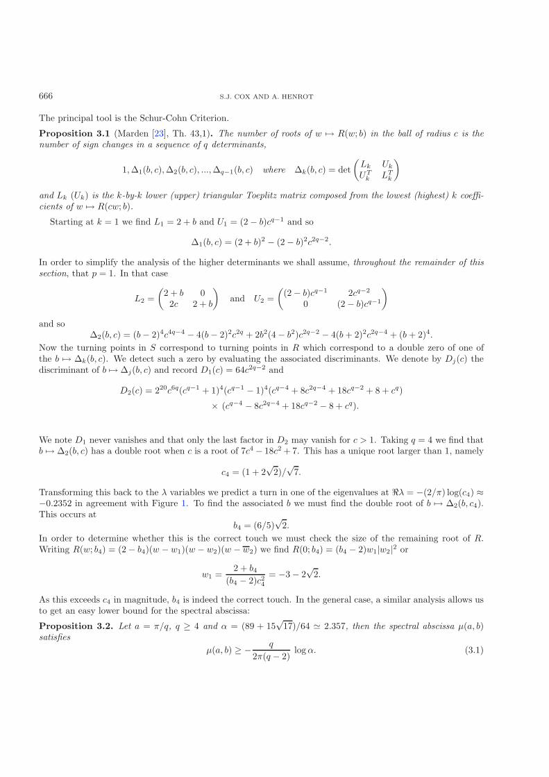
In the next 10 panels we have plotted the first q eigenvalues as a function of b as b ascends from 0 to 5 insteps of 0.01. For b < 2 we have used left-pointing arrowheads while for b > 2 we have used right-pointingarrowheads. We have, for greater legibility, limited the plot range real parts in excess of −2. We have placeda dashed vertical line at each minimal spectral abscissa. Each plot is labeled with its particular value of a andthe associated (approximate) minimal spectral abscissa, μ∗, and correct touch, b∗. These approximate valuesare obtained by solving the discrete minimization problem min{μ(a, k/100); k = 0 : 500}.

We shall now prove that the root trajectories indeed behave in the simple manner illustrated in Figure 1.Perhaps the first thing that catches one’s eye is the crossing of root trajectories when p and q are odd (panels(D, F, H) and (I)). We recall that though Bamberger et al. proved that all eigenvalues are geometrically simplethey neglected to consider higher algebraic multiplicity. The calculation is explicit when a = π/3. For

P (w; b) = (2 − b)w3 + bw + bw2 − (2 + b) = (w − 1)((2 − b)w2 + 2w + (2 + b))


−2 −1.5 −1 −0.5 00

2

4

6

8

(A) a = π/8, μ* = −0.0791, b

* = 2.79

−2 −1.5 −1 −0.5 00

1

2

3

4

(B) a = π/4, μ* = −0.235, b

* = 1.7

−2 −1.5 −1 −0.5 00

2

4

6

8

(C) a = 3π/8, μ* = −0.145, b

* = 3.02

−2 −1.5 −1 −0.5 00

1

2

3

4

5

6

7

(D) a = π/7, μ* = −0.0944, b

* = 2.49

−2 −1.5 −1 −0.5 00

1

2

3

4

5

6

7

(E) a = 2π/7, μ* = −0.129, b

* = 2.64

−2 −1.5 −1 −0.5 00

1

2

3

4

5

6

7

(F) a = 3π/7, μ* = −0.206, b

* = 2.69

Figure 1. Eigen-trajectories as a function of touch, b, for ten choices of site, a.

and the quadratic has roots at (−1 ±√b2 − 3)/(2 − b), that coincide at b =

√3. In terms of λ this states that

λ = (3/(2π)) ln(2−√3)+3i/2 is a double eigenvalue of A(π/3,

√3). It follows that b =

√3 is in fact the correct

touch when a = π/3.We now consider, for general a = pπ/q, the nature of incoming, splitting and outgoing branches along the

real axis and the line �(λ) = q/2.


−2 −1.5 −1 −0.5 00

1

2

3

4

5

6

(G) a = π/6, μ* = −0.117, b

* = 2.2

−2 −1.5 −1 −0.5 00

0.5

1

1.5

2

2.5

3

(H) a = π/3, μ* = −0.627, b

* = 1.73

−2 −1.5 −1 −0.5 00

1

2

3

4

5

(I) a = π/5, μ* = −0.156, b

* = 1.92

−2 −1.5 −1 −0.5 00

1

2

3

4

5

(J) a = 2π/5, μ* = −0.281, b

* = 2.11

Figure 1. Continued.

Proposition 2.1. We suppose a = pπ/q and λ = α+ iβ.(0) If b < 2 there exist no real eigenvalues. If b > 2 then there exists precisely one real eigenvalue α0(b). It

is strictly increasing with b and obeys

limb↓2

α0(b) = −∞ and limb→∞

α0(b) = 0.

(1) If q is even and b < 2 then α1(b) + iq/2 is an eigenvalue and α1(b) is strictly decreasing with b andobeys

limb↑2

α1(b) = −∞.

(2) If q is odd and p is even and b > 2 then α2(b) + iq/2 is an eigenvalue and α2(b) is strictly increasingwith b and obeys

limb↓2

α2(b) = −∞ and limb→∞

α2(b) = 0.

(3) If q is odd and p is odd then there exists a unique b∗ < 2 and α(b∗) such that a double eigenvalue occursat α(b∗) + iq/2. As b exceeds b∗ this eigenvalue splits into the pair α±(b) + iq/2 satisfying

α−(b) < α(b∗) < α+(b), limb↑2

α−(b) = −∞ and limb→∞

α+(b) = 0.


Proof.(0) If λ = α is real then (2.1) reads b = − sinh(απ)/(sinh(aα) sinh((π − a)α)). As this is strictly increasing

in α and takes values between 2 and ∞ the claim follows.(1) If q = 2n then S(α+in; p/(2n), b) = (−1)n{sinh(πα)+b cosh(aα) cosh((π−a)α)} and so b = − sinh(απ)/

(cosh(aα) cosh((π−a)α)). As this is strictly decreasing in α and takes values between 0 and 2 the claimfollows.

(2) At p = 2m, q = 2n + 1, S(α + iq/2; a, b) = i(−1)n{cosh(πα) + b cosh((π − a)α) sinh(aα)} and sob = − cosh(απ)/(sinh(aα) cosh((π − a)α)). As this is strictly increasing and takes values between 2and ∞ the claim follows.

(3) At p = 2m− 1, q = 2n+ 1, S(α+ iq/2; a, b) = i(−1)n{cosh(πα) + b cosh(aα) sinh((π − a)α)} and so

Fa(α) ≡ cosh(aα) sinh((π − a)α)cosh(πα)

= −1b· (2.5)

It is a simple matter to confirm

Fa(0) = 0, −1 ≤ Fa(α) ≤ 0, limα→−∞Fa(α) → −1/2

and that Fa has a unique critical point, αa, satisfying αa < −1/2. As this critical point is the global minimizerit follows that (2.5) has (i) no solution for b < ba ≡ −1/Fa(αa), (ii) one double root when b = ba, (iii) exactlytwo roots when ba < b < 2 (with one going to −∞ as b→ 2, and (iv) exactly one root when b > 2. �

We now show that this is the only possible multiple root.

Proposition 2.2. If λ is a root of S(·; a, b) then (i) its algebraic multiplicity can not exceed 2 and (ii) if it isdouble then �λ = q/2 mod q.

Proof. We note that S(λ; a, b) = sinh(πλ) + (b/2) cosh(πλ) − (b/2) cosh((π − 2a)λ) and so

S′′(λ; a, b) = π2 sinh(πλ) + π2(b/2) cosh(πλ) − (π − 2a)2(b/2) cosh((π − 2a)λ)

= π2S(λ; a, b) − ba(2a− π) cosh((π − 2a)λ)

and so if S(λ; a, b) = S′′(λ; a, b) = 0 then cosh((π−2a)λ) = 0. The latter requires that λ = i(n+1/2)π/(π−2a)but S(λ) �= 0.

For the second part we note that λ = −(q/(2π)) log(z) where z is a zero of P . We now show that everydouble root of P is real. If P (z) = P ′(z) = 0 then qP (z)−zP ′(z) = 0. Dividing the latter by bq and rearrangingbrings

tzq−p + (1 − t)zp = (b+ 2)/b, t = p/q (2.6)while z1−qP ′(z) = 0 brings

t/zq−p + (1 − t)/zp = (b − 2)/b. (2.7)If z1 ≡ zq−p and z2 ≡ zp then (2.6) and (2.7) require

t�(z1) + (1 − t)�(z2) = 0 and t�(z1)|z1|2 + (1 − t)

�(z2)|z2|2 = 0

and so either z1 and z2 are real or |z1| = |z2|. The latter is ruled out by the fact that |z| > 1. As zq−p andzp are both real and q − p and p are coprime it follows that z is real. This gives the desired result, sincez = exp(−2λπ/q). �

We now give a proposition which can be viewed as a “separation” result for the different branches of thespectrum.


Proposition 2.3. If a = pπ/q and b > 0 and b �= 2 then the spectrum does not hit the horizontal lines λ = α+iβwhere

β =k

2, k = 1, . . . , 2q − 1, k �= q

β = kq

2p, k = 1, . . . , 2p− 1, k �= p

β = kq

2(q − p), k = 1, . . . , 2(q − p) − 1, k �= q − p. (2.8)

Proof. We claim that if z is a root of (2.3) such that either zq or zp or zq−p is real, then necessarily z is real.This will give the result since z real means that the corresponding eigenvalue λ satisfies �λ = 0 or �λ = q/2 or�λ = q while the values of �λ appearing in (2.8) correspond to zq or zp or zq−p real (and z not real) and aretherefore forbidden. Now, if zp is real then

P (z; b) = zq

{(2 − b) +

b

zp

}+ bzp − (b + 2) = 0

immediately implies that zq is real. As p and q are coprime it follows that z real.Similarly, if zq−p is real then

P (z; b) = (2 − b)zq−pzp + bzp + bzq−p − (2 + b) = 0

implies that zp is real and so z is real.Next, if zq = t is real and zp = |z|peiθ then

P (z; b) = b|z|peiθ +bt

|z|p e−iθ + (2 − b)t− (b+ 2) = 0

implies that |z|peiθ + t|z|−pe−iθ is real. Now |z| > 1 implies that θ = 0, i.e., zp real, and so z itself is real. �Recalling Figure 1 we set r = max(p, q − p) and distinguish the exit trajectories (where the magnitude of

the real part is an unbounded increasing function of 0 < b < 2) and return trajectories (where the magnitudeof the real part is an unbounded decreasing function of 2 < b <∞) from the finite loops (bounded trajectory).Note that q − r = min(p, q − p) and that q − 2r < 0.

For the behavior of the branches as b→ +∞, we easily see (for example by writing the polynomial equation(1−zr)(1−zq−r) = 2(1−zq)/b), that the limit of all the branches are the points on the imaginary axis given by

λ = imq

r, m = 0, . . . , r − 1

λ = imq

q − r, m = 0, . . . , q − r − 1.

We will see below that the first values are the end points of the finite loops, while the other ones are the endpoints of return trajectories.

Now, at b = 2 we have only r roots so q − r roots must escape as b ↑ 2. To follow these we write

P (z; b) = zr{(2 − b)zq−r + b+ bzq−2r − (b+ 2)z−r} = 0

and deduce when |z| → +∞ that zq−r ∼ bb−2 . When b ↑ 2, it follows that

z ∼(

b

2 − b

)1/(q−r)

exp(iπ(1 + 2m)/(q − r)), m = 0, 1, . . . , q − r − 1.


Therefore, the possible imaginary parts of the exit trajectories (b ↑ 2) are

β =q

2(q − r)(1 + 2m), m = 0, 1, . . . , q − r − 1. (2.9)

Similarly, the return trajectories (b ↓ 2) emanate from points with imaginary part

β = mq

q − r, m = 0, 1, . . . , q − r − 1.

We now combine (2.9) with Proposition 2.3 to locate the starting points of the exit trajectories. Indeed, the firststatement of (2.8) shows that there exists horizontal lines that the spectrum cannot cross every i/2. Therefore,the only possible starting point for the trajectory that exits at iβ, where β = q(1+2m)/(2(q− r)), is i round(β)where round returns the closest integer. This is well defined except when β is exactly half of an odd integer.Since q − r is coprime with q, this can only happen if q − r divides 2m+ 1. But, since 2m+ 1 < 2(q − r), theonly possible case is 2m + 1 = q − r. In this case, Proposition 2.1(3) instructs us that the branch is exactlythe half-line β = q/2 and it comes from both (q + 1)i/2 and (q − 1)i/2. Without loss we identify the lowerpoint, (q− 1)i/2, with starting point of the loop that ends at iq/2 after splitting, and identify the upper point,(q + 1)i/2, as the starting point of the trajectory that exits the complex plane at β = q/2 after splitting. Wehave now proven:

Proposition 2.4. We set r ≡ max{p, q − p} and denote by round± the extension of round for whichround−(1/2) = 0 and round+(1/2) = 1.

(1) There exist r − 1 proper loops, m(b), 0 ≤ b ≤ ∞,

m(∞) = imq/r and m(0) = i round−(mq/r), m = 1, . . . , r − 1.

These are smooth where they avoid the multiple eigenvalue.(2) There exist q − r exit trajectories, εj(b), 0 ≤ b ≤ 2,

�εj(2−) =q(1 + 2j)2(q − r)

and εj(0) = i round+

(q(1 + 2j)2(q − r)

), j = 0, . . . , q − r − 1.

These are smooth where they avoid the multiple eigenvalue.(3) There exist q − r smooth return trajectories, ρj(b), 2 ≤ b ≤ ∞,

�ρj(2+) =jq

q − rand ρj(0) = i round

(jq

q − r

), j = 0, . . . , q − r − 1.

It follows that the nonharmonic spectral abscissa, b → μ(pπ/q, b) of (1.5), is continuous and bounded belowon [0,∞] and μ(pπ/q,∞) = 0. Hence, there exists a correct touch, i.e.:

Corollary 2.1. For integer coprime p and q the function b → μ(pπ/q, b) attains its minimum over [0,∞] at afinite value b∗(p, q).

Perusal of the root trajectories in Figure 1 suggests that b∗ occurs at a turning point (vertical tangent) ofthe smallest loop or perhaps along the fastest return trajectory. We now proceed to bound these loops.

3. Bounds on µ and b∗

We apply the determinant methods of Schur and Cohn to bound the moduli of the roots of

R(w; b) = P (w; b)/(w − 1) = (2 + b)p−1∑j=0

wj + 2q−p−1∑

j=p

wj + (2 − b)q−1∑

j=q−p

wj .


The principal tool is the Schur-Cohn Criterion.

Proposition 3.1 (Marden [23], Th. 43,1). The number of roots of w → R(w; b) in the ball of radius c is thenumber of sign changes in a sequence of q determinants,

1,Δ1(b, c),Δ2(b, c), ...,Δq−1(b, c) where Δk(b, c) = det(Lk Uk

UTk LT

k

)

and Lk (Uk) is the k-by-k lower (upper) triangular Toeplitz matrix composed from the lowest (highest) k coeffi-cients of w → R(cw; b).

Starting at k = 1 we find L1 = 2 + b and U1 = (2 − b)cq−1 and so

Δ1(b, c) = (2 + b)2 − (2 − b)2c2q−2.

In order to simplify the analysis of the higher determinants we shall assume, throughout the remainder of thissection, that p = 1. In that case

L2 =(

2 + b 02c 2 + b

)and U2 =

((2 − b)cq−1 2cq−2

0 (2 − b)cq−1

)

and soΔ2(b, c) = (b− 2)4c4q−4 − 4(b− 2)2c2q + 2b2(4 − b2)c2q−2 − 4(b+ 2)2c2q−4 + (b + 2)4.

Now the turning points in S correspond to turning points in R which correspond to a double zero of one ofthe b → Δk(b, c). We detect such a zero by evaluating the associated discriminants. We denote by Dj(c) thediscriminant of b → Δj(b, c) and record D1(c) = 64c2q−2 and

D2(c) = 220c6q(cq−1 + 1)4(cq−1 − 1)4(cq−4 + 8c2q−4 + 18cq−2 + 8 + cq)

× (cq−4 − 8c2q−4 + 18cq−2 − 8 + cq).

We note D1 never vanishes and that only the last factor in D2 may vanish for c > 1. Taking q = 4 we find thatb → Δ2(b, c) has a double root when c is a root of 7c4 − 18c2 + 7. This has a unique root larger than 1, namely

c4 = (1 + 2√

2)/√

7.

Transforming this back to the λ variables we predict a turn in one of the eigenvalues at �λ = −(2/π) log(c4) ≈−0.2352 in agreement with Figure 1. To find the associated b we must find the double root of b → Δ2(b, c4).This occurs at

b4 = (6/5)√

2.In order to determine whether this is the correct touch we must check the size of the remaining root of R.Writing R(w; b4) = (2 − b4)(w − w1)(w − w2)(w − w2) we find R(0; b4) = (b4 − 2)w1|w2|2 or

w1 =2 + b4

(b4 − 2)c24= −3 − 2

√2.

As this exceeds c4 in magnitude, b4 is indeed the correct touch. In the general case, a similar analysis allows usto get an easy lower bound for the spectral abscissa:

Proposition 3.2. Let a = π/q, q ≥ 4 and α = (89 + 15√

17)/64 � 2.357, then the spectral abscissa μ(a, b)satisfies

μ(a, b) ≥ − q

2π(q − 2)logα. (3.1)


Proof. As mentioned above, a turning point may arrive for a value of c such that

E(c) ≡ −8c2q−4 + cq + 18cq−2 + cq−4 − 8 = 0 .

Following the rule of signs of Descartes [23], Theorem 41.3, we know that the number n of positive zeros andthe number m of change of signs in the coefficient of E satisfy n ≤ m and m− n even. Since m = 2, E(0) < 0,E(1) > 0 and E(+∞) < 0, it follows that E has two positive zeros and only one of them being larger than 1.More precisely, since E(2) can be written E(2) = −8 ∗ 22q−4 + 89

4 2q−2 − 8 and 8 ∗ 2q−2 > 894 for q ≥ 4, we see

that the unique root of E, say cq, larger than 1 is smaller than 2. We use this fact to improve the bound on cq.Since

c2q + 18 + 1/c2q < 22 + 18 + 1/22 = 89/4we get

0 = E(cq) < −8c2q−4q +

894cq−2q − 8

and the bound cq−2q < α follows immediately. As the entire loop stays inside the disk of radius cq the bound (3.1)

stems from the link between the modulus of w and �(λ). �

It is also possible to get a lower bound for the spectral abscissa in terms of b. For that purpose, let usobserve that looking at Δ1(b, c), we immediately obtain that it becomes negative when c crosses the value((2+b)/(2−b))1/(q−1), therefore the polynomial R has at least one root in the disk |w| < ((2+b)/(2−b))1/(q−1).Of course, if we now consider the next determinant Δ2(b, c), we can improve this upper bound.

We factor Δ2(b, c) into

Δ2(b, c) =((b− 2)2c2(q−1) + 2(b− 2)cq + 2(b+ 2)cq−2 − (b+ 2)2

)×((b− 2)2c2(q−1) − 2(b− 2)cq − 2(b+ 2)cq−2 − (b+ 2)2

)≡ Q1(b, c)Q2(b, c)

and look for the first zero of either Q1 or Q2. We observe that Q2(b, c) ≤ Q1(b, c) while (b−2)cq+(b+2)cq−2 ≥ 0,i.e.

Q2(b, c) ≤ Q1(b, c) ⇐⇒ b ≥ 2 or

{b < 2 and 1 ≤ c ≤

(2 + b

2 − b

)1/2}.

Now, since

Q1(b, 1) < 0 and Q1

(b,

(2 + b

2 − b

)1/2)

= (b+ 2)2((

2 + b

2 − b

)q−3

− 1

)> 0

the first zero of Q1 (and therefore of P ) is less than ((2 + b)/(2 − b))1/2 and, therefore, we can assume that weare in the case Q2(b, c) ≤ Q1(b, c). At last, since Q1(b, 1) = −4b < 0 and Q2(b, 1) = −12b < 0, Q1(b, c) willvanish before Q2(b, c), so we can restrict ourselves to the study of Q1(b, c).

We begin with the case b ≥ 2. Let z0 be the positive root of

R2(z) ≡ (b− 2)2z2 + [2(b− 2) + 2(b+ 2)]z − (b+ 2)2.

Namely, z0 = (−2b +√b4 − 4b2 + 16)/(b − 2)2 for b �= 2, and z0 = 2 for b = 2. We note that z0 > 1, set

c0 ≡ z1/(q−2)0 > 1 and observe that if b ≥ 2 then

Q1(b, c0) = (b − 2)2c20z20 + 2(b− 2)c20z0 + 2(b+ 2)z0 − (b+ 2)2

≥ (b − 2)2z20 + 2(b− 2)z0 + 2(b+ 2)z0 − (b+ 2)2 = 0.

Therefore, c0 is an upper bound for the first zero of P when b ≥ 2.


0 1 2 3 4 5 6 7 8 9 10−0.16

−0.14

−0.12

−0.1

−0.08

−0.06

−0.04

−0.02

0

b

μ

Figure 2. Estimate from above (solid line) for the spectral abscissa (dashed line) in the casea = π/10.

We use the same kind of method in the case b < 2. We introduce z1 the (unique) positive root of

R3(z) ≡ (b− 2)2z3 + 2(b− 2)z2 + 2(b+ 2)z − (b+ 2)2 = 0.

Since R3(1) = −4b < 0 and R3(2/(2 − b)) = b2(b + 2)/(2 − b) > 0 we see that 1 < z1 < 2/(2 − b). We setc1 ≡ z

1/(q−2)1 and observe that if b ≤ 2 then

Q1(b, c1) = (b − 2)2c21z21 + 2(b− 2)c21z1 + 2(b+ 2)z1 − (b+ 2)2

= c21z1(b − 2)[(b− 2)z1 + 2] + 2(b+ 2)z1 − (b+ 2)2

≥ z21(b− 2)[(b− 2)z1 + 2] + 2(b+ 2)z1 − (b+ 2)2 = 0

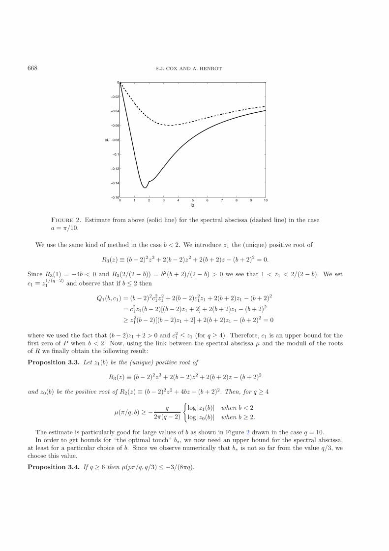
where we used the fact that (b− 2)z1 + 2 > 0 and c21 ≤ z1 (for q ≥ 4). Therefore, c1 is an upper bound for thefirst zero of P when b < 2. Now, using the link between the spectral abscissa μ and the moduli of the rootsof R we finally obtain the following result:

Proposition 3.3. Let z1(b) be the (unique) positive root of

R3(z) ≡ (b− 2)2z3 + 2(b− 2)z2 + 2(b+ 2)z − (b + 2)2

and z0(b) be the positive root of R2(z) ≡ (b− 2)2z2 + 4bz − (b + 2)2. Then, for q ≥ 4

μ(π/q, b) ≥ − q

2π(q − 2)

{log |z1(b)| when b < 2log |z0(b)| when b ≥ 2.

The estimate is particularly good for large values of b as shown in Figure 2 drawn in the case q = 10.In order to get bounds for “the optimal touch” b∗, we now need an upper bound for the spectral abscissa,

at least for a particular choice of b. Since we observe numerically that b∗ is not so far from the value q/3, wechoose this value.

Proposition 3.4. If q ≥ 6 then μ(pπ/q, q/3) ≤ −3/(8πq).


Proof. We outline the key steps but suppress the many routine calculations. We recall the S of (2.2) and setφ(α, β) ≡ |S(α+ iβ)|2. We begin by working with β fixed in the range of possible values corresponding to thedifferent branches of the spectrum. We denote by B this set of possible values for β. We will often need toseparate the cases of the closed loops and branches returning from infinity.

Step 1. The function α → φα(α, β) is non decreasing for −1/(πq) ≤ α ≤ 0 (we just need to compute thesecond derivative φαα(α, β) which is clearly non negative).

Step 2. The inequalities φα(0, β) ≥ 0 and φα(−1/(πq), β) + φα(0, β) ≥ 0 hold. Actually, it is the longer andmore technical part of the proof. For that, we write

1π

(φα

(−1πq, β

)+ φα(0, β)

)= A+B1

p

3cos

2(q − p)q

βπ +B2q − p

3cos

2pqβπ (3.2)

with

A =q

3+q

3cosh

2q− (1 +

q2

36) sinh

2q− q(q − 2p)

36sinh

2(q − 2p)q2

B1 = −1 +q

6sinh

2pq2

− cosh2pq2

B2 = −1 +q

6sinh

2(q − p)q2

− cosh2(q − p)q2

and we get the result using classical inequalities satisfied by the functions cosh and sinh and precise study ofthe function of β defined in (3.2).

Step 3. We deduce from steps 1 and 2 that |φα(α, β)| ≤ φα(0, β) for −1/(πq) ≤ α ≤ 0 and so φ(0, β)−φ(α, β) ≤φα(0, β)|α| there and then, φ(α, β) (and also S) cannot vanish while

φ(0, β) − φα(0, β)|α| > 0 ⇐⇒ |α| < φ(0, β)φα(0, β)

≡ ψ(β).

As a consequence, the spectral abscissa μ satisfies μ ≤ −ψ(β) for each β ∈ B.

Step 4. We find a lower bound for

ψ(β) =sin2 βπ + q2

9 sin2 pqβπ sin2 (q−p)

q βπ

2π(

p3 sin2 q−p

q βπ + q−p3 sin2 p

qβπ) (3.3)

when β varies in the range of possible values. We now examine separately the case of a closed loop and the caseof a branch coming back from infinity (since b = q/3 ≥ 2, we do not need to look at the case of a branch goingto infinity). For sake of simplicity, we assume here that r = q− p (i.e. q ≥ 2p). The proof would be exactly thesame in the other case.

The case of a loop finishing at imq/(q−p) corresponds to values of β belonging to the interval(k, mq

q−p

)with

k ≡ round(mq/(q − p)) and m are connected by a relation like mq − k(q − p) = m0. Now, we use that on suchan interval sin2((π − a)β) ≤ sin2(aβ) to get

ψ(β) ≥ 32πq

(q2

9sin2((π − a)β) +

sin2 βπ

sin2(aβ)

)· (3.4)


We split the interval I =(k, mq

q−p

)into I =

(k, k + 1

2m0q−p

)∪(k + 1

2m0q−p , k + m0

q−p

)= I1 ∪ I2. On I1, we have

ψ(β) ≥ 32πq

q2

9sin2 q − p

qβπ ≥ q

6πsin2 q − p

q

(k +

12m0

q − p

)π =

q

6πsin2 m0π

2q·

At last, since on [0, π/12], sin2 x ≥ ( 12xπ sin π

12

)2, we get

sin2 m0π

2q≥ sin2 π

2q≥ 144

π2

π2

4q2sin2 π

12=

18q2

(1 −

√3

2

),

therefore, on I1

ψ(β) ≥ 3(2 −√3)

2πq· (3.5)

On I2, we write:

ψ(β) ≥ 32πq

sin2 βπ

sin2 pqβπ

≥ 32πq

sin2(kπ + 12

m0πq−p )

sin2 pπq (k + m0

q−p ),

the right-hand side is equal to3

2πq

sin2 m0π2(q−p)

sin2 m0π(q−p)

=3

2πq1

4 cos2 m0π2(q−p)

therefore, on I2

ψ(β) ≥ 38πq

· (3.6)

In the case of a branch coming back from infinity, which corresponds to an interval like(k, jq

q−r

)with k ≡

round(jq/(q − r)) and jq − k(q − r) = q − j0, we use the same idea and we get the same inequalities as (3.5)and (3.6). �

As a consequence of the upper and lower bounds on the nonharmonic spectral abscissa we obtain the followingbounds on the correct touch.

Proposition 3.5. Let us denote by b∗(p, q) the correct touch, i.e., the minimizer of b → μ(pπ/q, b). If p = 1and q ≥ 6 then

b1(q) ≤ b∗(p, q) ≤ b2(q) (3.7)

where

b1(q) =2z3 − z2 − z + 2 +

√−7z4 + 18z3 − 7z2

z3 − 1

b2(q) =2(z2 − z + 1) + 2

√2z(2 − z)(z − 1

2 )

z2 − 1

and z = exp(3(q − 2)/4q2

).

Proof. To find these bounds, it suffices to look at the intersection of the curve giving the lower bound with theline μ = −3/(8πq). Or, equivalently, to find b such that (in the language of Prop. 3.3) z0(b) and z1(b) equalexp

(3(q − 2)/4q2

). We obtain the result by plugging this value of z in the equation defining z0(b) and z1(b)

respectively and solving in b. �


4. Regarding the root vectors

Recall that Rayleigh was already aware of the fact that pointwise damping destroys the “normal co-ordinates”or orthonormal basis of eigenmodes enjoyed by the undamped wave operator. For our purposes however it willsuffice to show that the (generalized) eigenmodes, or root vectors, are isomorphic to an orthonormal base. Inother words, we show that these modes comprise a Riesz basis for the energy space, X . We begin with aspecification of these modes.

In addition to the harmonic modes in (1.2) we have the nonharmonic modes

Vk,n(x) = yk,n(x)[1/λk,n 1], yk,n(x) =

{sinh(λk,n(π − a)) sinh(λk,nx) if x < a,

sinh(λk,na) sinh(λk,n(π − x)) if x > a,(4.1)

where k = 2, . . . , q and n runs through the integers.If λk,n = λk+1,n then, in addition to its eigenvector Vk,n, there exists the generalized eigenvector Vk+1,n = [y z]

for which (A− λk)Vk+1,n = Vk,n. In components this reads

z = λk,ny + yk,n/λk,n and y′′ − (λk,n + bδa)z = yk.

The first into the latter yields

y′′ − λ2k,ny − λk,nbδay = (2 + bδa/λk,n)yk,n

that is, y is the H10 (0, π) function satisfying

y′′ − λ2k,ny = 2

{sinh(λk,n(π − a)) sinh(λk,nx) if x < a,

sinh(λk,na) sinh(λk,n(π − x)) if x > a,(4.2)

and the transmission condition

y′(a+) − y′(a−) = λk,nbyk,n(a) + byk,n(a)/λk,n. (4.3)

The solution to (4.2)–(4.3) is, piecewise,

y(x) =1λk,n

{(π − a) cosh(λk,n(π − a)) sinh(λk,nx) + x cosh(λk,nx) sinh(λk,n(π − a))a cosh(λk,na) sinh(λk,n(π − x)) + (π − x) cosh(λk,n(π − x)) sinh(λk,na)

We now show that the root vectors comprise a Riesz Basis for X . In some related cases, e.g., Kergo-mard et al. [17], the underlying isomorphism can be constructed by hand. We follow here the indirect ap-proach of Bari, e.g., Young [34], Theorem 1.9, and show that they comprise a complete Bessel sequence andare biorthogonal to a set that is also complete and Bessel. To begin, as {V1,n}n=0 is an orthonormal sequencein X , Bessel’s inequality reads

±∞∑n=±1

|〈V1,n, V 〉|2 ≤ ‖V ‖2, ∀V ∈ X

and so we need only show:

Proposition 4.1. If V ∈ X then∑

n

|〈Vk,n, V 〉|2 <∞ for each k = 2, . . . , q.


Proof. We write V = [y z] and find

〈Vk,n, V 〉 = (1/λk,n)∫ π

0

y′k,ny′ dx+

∫ π

0

yk,nz dx. (4.4)

Now, as λk,n = λk,0 − iqn,

1λk,n

∫ π

0

y′k,ny′ dx = (−1)n(q−p) sinh(λk,0(π − a))

∫ a

0

cosh((λk,0 − inq)x)y′(x) dx

− (−1)np sinh(λk,0a)∫ π

a

cosh((λk,0 − inq)(π − x))y′(x) dx. (4.5)

As {nq}n is a separated sequence it follows from Young [34], Theorem 4.4, that einq is a Bessel sequencein L2(−π, π) and hence the sequence (4.5) is square summable in n. This same argument allows us to concludethat the second term in (4.4) is also square summable in n. Finally, given our explicit representation of the rootvectors associated with double eigenvalues, the argument above may be used to show that these too constitutea Bessel sequence. �

These same estimates hold for the adjoint system

A∗(a, b) =(

0 −I−∂xx 0

)x �= a

D(A∗(a, b)) = {[f, g] ∈ (H10 (0, π) ∩H2(0, a) ∩H2(a, π)) ×H1

0 (0, π) : f ′(a+) − f ′(a−) = −bg(a)}

for its root vectors are Wk,n(x) = yk,n(x)[1/λk,n − 1]. It is a simple matter to confirm that this sequence isbiorthogonal to {Vk,n}.

Regarding completeness, as our pointwise damping is an unbounded ‘perturbation’ of the skew wave operatorwe may not argue as in Cox and Zuazua [9]. Instead, following Krein and Nudelman [20], Cox and Zuazua [10]and Ammari et al. [1], we invoke the simple trace criterion of Livsic.

Proposition 4.2 (Krein and Langer [19], Sect. 2.5). If H is Hilbert and T : H → H is linear and compact andT ≡ (T + T ∗)/2 is nonpositive and of finite trace then

tr(T) ≤∑

νn∈σ(T)

�νn (4.6)

where the νn are repeated according to their algebraic multiplicity. Equality holds in (4.6) if and only if the rootvectors of T are complete in H.

It is now a simple matter to confirm that equality holds in (4.6). We note that an alternate route tocompleteness has recently been established in the works of Guo and Xie [14] and Xu and Guo [33].

Proposition 4.3. tr(A−1(a, b)) = −b(π − a)a/π.

Proof. If [f g] = A−1(a, b)[u v] then g = u and f ′′ = v + bδau with f(0) = f(π) = 0. Hence

f(x) =∫ x

0

(x− t)v(t) dt − (x/π)∫ π

0

(π − t)v(t) dt − (b/π)u(a)ψ(x)

where

ψ(x) =

{(π − a)x if x < a,

a(π − x) if x > a.


Similarly, if [f g] = A−1(a, b)∗[u v] then g = −u and f ′′ = −v + bδau with f(0) = f(π) = 0. Hence, as above

f(x) = −∫ x

0

(x− t)v(t) dt+ (x/π)∫ π

0

(π − t)v(t) dt− (b/π)u(a)ψ(x).

Combining these calculations we find A−1(a, b)[u v] = [−(b/π)u(a)ψ 0], and so the range of A−1(a, b) isspanned by the unit vector e1 ≡ [ψ 0]/

√aπ(π − a). The claim follows from trA−1(a, b) = 〈A−1(a, b)e1, e1〉.

�The polynomial representation of our shooting function affords the elementary factorization

S(λ; pπ/q, b) = −14

exp(λπ)P (exp(−2πλ/q); b)

=14

exp(λπ)(b − 2)q∏

k=1

(exp(−2πλ/q) − wk). (4.7)

The beauty of this representation is that sums of eigenvalues, as required by (4.6), appear on differentiationwith respect to λ. The computation of these sums will be facilitated by

∑n

1(n+ α)2 + β2

=π

2βsinh(2πβ)

cosh2(πβ) − cos2(πα)(4.8)

that follows by summing the residues of −π cot(πz)/((z + α)2 + β).

Proposition 4.4. If b ≥ 0 and b �= 2 then the shooting function satisfies

S(λ; pπ/q, b) = πλ− πλ2

q∑k=1

∑n

�(1/λk,n) +O(λ3).

Proof. We simply differentiate (4.7) with respect to λ and make frequent use of the fact that w1 = 1. To begin,with a = pπ/q,

Sλ(λ; a, b) =π

4eλπ(b− 2)

q∏k=1

(e−2πλ/q − wk) − π

2qeλπ(1−2/q)(b − 2)

q∑j=1

∏k =j

(e−2πλ/q − wk).

The first term vanishes at λ = 0 and the products in the second term each vanish except when j = 1. Hence

Sλ(0; a, b) =π

2q(2 − b)

q∏k=2

(1 − wk) =π

2qP (w)w − 1

∣∣∣∣w=1

= π

as claimed. Proceeding to the second derivative

Sλλ(λ; a, b) =π2

4eλπ(b − 2)

q∏k=1

(e−2πλ/q − wk)

− π2(q − 1)q2

eλπ(1−2/q)(b − 2)q∑

j=1

∏k =j

(e−2πλ/q − wk)

+π2

q2eλπ(1−4/q)(b− 2)

q∑j=1

q∑i=1

∏k ∈{i,j}

(e−2πλ/q − wk).


At λ = 0 this becomes

Sλλ(0; a, b) =π2(q − 1)

q2(2 − b)

q∏k=2

(1 − wk) +2π2

q2(b − 2)

q∑j=2

∏k ∈{1,j}

(1 − wk)

=2π2(q − 1)

q− 4π2

q

q∑k=2

11 − wk

=2π2

q

q∑k=2

(1 − wk

1 − wk− 2

1 − wk

)

=2π2

q

q∑k=2

wk + 1wk − 1

(4.9)

and so it remains only to link the wk back to their λk,n. Well, it follows directly from (2.4) that

�(1/λk,n) =− log |wk|

2πq1

log2(|wk|)/(4π2) + (n+ θk/(2π))2·

With α = θk/(2π) and β = log(|wk|)/(2π) it now follows from (4.8) that

∑n

�(1/λk,n) =− log |wk|

2πqπ2

log |wk|sinh(log |wk|)

cosh2(log(|wk|)/2) − cos2(θk/2)

=−π4q

|wk| − |wk|−1

(|wk| + 2 + |wk|−1)/4 − cos2(θk/2)

=π

q

1 − |wk|2|wk|2 − 2�wk + 1

· (4.10)

In order to reconcile (4.10) and (4.9) we note that if wk is real then

1 − |wk|2|wk|2 − 2�wk + 1

=wk + 11 − wk

while if wk is not real then

1 − |wk|2|wk|2 − 2�wk + 1

+1 − |wk|2

|wk|2 − 2�wk + 1=wk + 11 − wk

+wk + 11 − wk

·

As each wk is either real or occurs with its complex conjugate, we have shown,

Sλλ(0; a, b) = −2πq∑

k=1

∑n

�(1/λk,n)

as claimed. �

Comparing now the MacLaurin developments of S as represented in (2.1) and the above proposition, we find

πλ+ b(π − a)aλ2 +O(λ3) = πλ − πλ2∑

λn∈σ(a,b)

�(1/λn) +O(λ3)


−4 −3.5 −3 −2.5 −2 −1.5 −1 −0.5 00

1

2

3

4

5

6

7

8

9

10

11

real

imag

inar

y

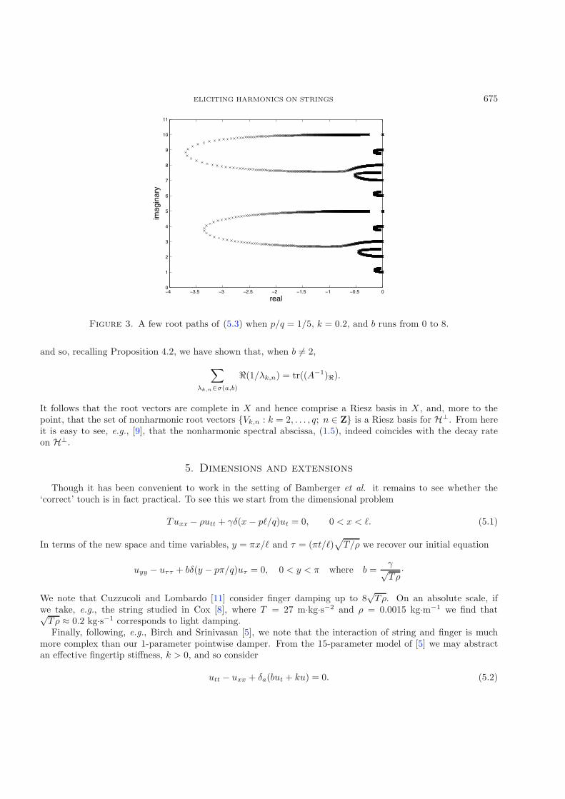
Figure 3. A few root paths of (5.3) when p/q = 1/5, k = 0.2, and b runs from 0 to 8.

and so, recalling Proposition 4.2, we have shown that, when b �= 2,

∑λk,n∈σ(a,b)

�(1/λk,n) = tr((A−1)).

It follows that the root vectors are complete in X and hence comprise a Riesz basis in X , and, more to thepoint, that the set of nonharmonic root vectors {Vk,n : k = 2, . . . , q; n ∈ Z} is a Riesz basis for H⊥. From hereit is easy to see, e.g., [9], that the nonharmonic spectral abscissa, (1.5), indeed coincides with the decay rateon H⊥.

5. Dimensions and extensions

Though it has been convenient to work in the setting of Bamberger et al. it remains to see whether the‘correct’ touch is in fact practical. To see this we start from the dimensional problem

Tuxx − ρutt + γδ(x− p/q)ut = 0, 0 < x < . (5.1)

In terms of the new space and time variables, y = πx/ and τ = (πt/)√T/ρ we recover our initial equation

uyy − uττ + bδ(y − pπ/q)uτ = 0, 0 < y < π where b =γ√Tρ

·

We note that Cuzzucoli and Lombardo [11] consider finger damping up to 8√Tρ. On an absolute scale, if

we take, e.g., the string studied in Cox [8], where T = 27 m·kg·s−2 and ρ = 0.0015 kg·m−1 we find that√Tρ ≈ 0.2 kg·s−1 corresponds to light damping.Finally, following, e.g., Birch and Srinivasan [5], we note that the interaction of string and finger is much

more complex than our 1-parameter pointwise damper. From the 15-parameter model of [5] we may abstractan effective fingertip stiffness, k > 0, and so consider

utt − uxx + δa(but + ku) = 0. (5.2)


This breaks the lovely symmetry of the shooting function,

S(λ; a, b) = λ sinh(λπ) + (bλ+ k) sinh(λa) sinh(λ(π − a)). (5.3)

and so also destroys the simple structure of the spectrum. In comparing Figures 1 and 3 we see at once boththe unfolding of the multiple eigenvalue and the genesis of the exit and return trajectories. Although theqi periodicity is broken, it appears that the full spectral abscissa is attained on one of the first q trajectories.

It remains of course to determine whether the correct touch in the sense of Bamberger, Rauch and Tayloris indeed the most pleasing to the ear. If in fact the nonharmonic spectral abscissa is the right measure tominimize then Figure 1 seems to indicate a number of improvements over current practice. More precisely,modern practice, as dictated by Zukovsky [36], has the musician lightly finger at /q and yet, for odd q > 3Figure 1 states that fingering at 2/q is better, i.e., μ(2/q, b∗(2, q)) < μ(/q, b∗(1, q)). By this reasoning itappears that touching simultaneously at /q and 2/q should in turn further enhance the effect.

References

[1] K. Ammari, A. Henrot and M. Tucsnak, Asymptotic behavior of the solutions and optimal location of the actuator for thepointwise stabilization of a string. Asymptot. Anal. 28 (2001) 215–240.

[2] A. Bamberger, J. Rauch and M. Taylor, A model for harmonics on stringed instruments. Arch. Rational Mech. Anal. 79 (1982)267–290.

[3] G. Banat, Masters of the Violin, Sonatas for the Violin, Jean-Joseph Cassanea de Mondonville 5. Johnson Reprint (1982).

[4] D. Bernoulli, Reflexions et eclaircissemens sur les nouvelles vibrations des cordes exposees dans les memoires de 1747 and 1748.Histoire de l’Academie royale des sciences et belles lettres 9 (1753) 148–172.

[5] A.S. Birch and M.A. Srinivasan, Experimental determination of the viscoelastic properties of the human fingerpad. Touch LabReport 14, RLE TR-632, MIT, Cambridge (1999).

[6] J.T. Cannon and S. Dostrovsky, The Evolution of Dynamics, Vibration Theory from 1687 to 1742. Springer, New York (1981).[7] T. Christensen, Rameau and Musical Thought in the Enlightenment. Cambridge (1993).[8] S.J. Cox, Aye there’s the rub, An inquiry into how a damped string comes to rest, in Six Themes on Variation, R. Hardt Ed.,

AMS (2004) 37–58.[9] S. Cox and E. Zuazua, The rate at which energy decays in a damped string. Comm. Partial Diff. Eq. 19 (1994) 213–243.

[10] S. Cox and E. Zuazua, The rate at which energy decays in a string damped at one end. Indiana U. Math. J. 44 (1995) 545–573.[11] G. Cuzzucoli and V. Lombardo, A physical model of the classical guitar, including the player’s touch. Comput. Music J. 23

(1999) 52–69.[12] F.W. Galpin, Monsieur Prin and his trumpet marine. Music Lett. 14 (1933) 18–29.[13] C. Girdlestone, Jean-Philippe Rameau. Cassell, London (1957).[14] B.-Z. Guo and Y. Xie, A sufficient condition on Riesz basis with parenthesis of nonself-adjoint operator and application to a

serially connected string system under joint feedbacks. SIAM J. Control Optim. 43 (2004) 1234–1252.[15] H. Helmholtz, On the Sensations of Tone. Dover (1954).[16] S. Jaffard, M. Tucsnak and E. Zuazua, Singular internal stabilization of the wave equation. J. Diff. Eq. 145 (1998) 184–215.[17] J. Kergomard, V. Debut and D. Matignon, Resonance modes in a 1-D medium with two purely resistive boundaries: calculation

methdos, orthogogonality and completeness. J. Acoust. Soc. Am. 119 (2006) 1356–1367.[18] I. Kovacs, Zur Frage der Seilschwingungen und der Seildampfung. Die Bautechnik 59 (1982) 325–332.[19] M.G. Krein and H. Langer, On some mathematical principles in the linear theory of damped oscillations of continua I. Integr.

Equ. Oper. Theory 1 (1978) 364–399.[20] M.G. Krein and A.A. Nudelman, On direct and inverse problems for the boundary dissipation frequencies of a nonuniform

string. Soviet Math. Dokl. 20 (1979) 838–841.[21] S. Krenk, Vibrations of a taut cable with an external damper. J. Appl. Mech. 67 (2000) 772–776.[22] K.S. Liu, Energy decay problems in the design of a pointwise stabilizer for string vibrating systems. SIAM J. Control Optim.

26 (1988) 1248–1256.[23] M. Marden, Geometry of Polynomials. AMS (1966).[24] D.C. Miller, Anecdotal History of the Science of Sound. Macmillan, New York (1935).[25] J.-P. Rameau, Generation Harmonique, Facsimile of 1737 Paris Ed., Broude Brothers, New York (1966).[26] J.W.S. Rayleigh, Theory of Sound, Vol. 1. Dover (1945).[27] F. Roberts, A discourse concerning the musical notes of the trumpet, and trumpet-marine, and of the defects of the same.

Philosophical Transactions 16 (1692) 559–563.[28] J. Sauveur, Systeme general des intervalles des sons et son application a tous les systemes et a tous les instrumens de musique,

Memoires de l’Academie royale des sciences 1701. Amsterdam (1707) 390–482.


[29] B. Taylor, De Moti Nervi Tensi. Philosophical Transactions 28 (1713) 26–32.[30] C. Truesdell, The Rational Mechanics of Flexible or Elastic Bodies, 1638–1788, introduction to Leonhardi Euleri Opera Omnia

Vols. 10 and 11, Series 2, Leipzig (1912).[31] J. Tyndall, Sound. D. Appleton (1875).[32] J. Wallis, Concerning a new musical discovery. Philosophical Transactions 12 (1677) 839–842.[33] G.-Q. Xu and B.-Z. Guo, Riesz basis property of evolution equations in Hilbert spaces and application to a coupled string

equation. SIAM J. Control Optim. 42 (2003) 966–984.[34] R.M. Young, An Introduction to Nonharmonic Fourier Series. Academic Press, San Diego (2001).[35] T. Young, A Course of Lectures on Natural Philosophy and the Mechanical Arts. Johnson Reprint (1971).[36] P. Zukovsky, On violin harmonics. Perspectives of New Music 6 (1968) 174–181.

Steven J. Cox and Antoine Henrot...Steven J. Cox1 and Antoine Henrot2 Abstract. One may produce the...

Documents

Transcript of Steven J. Cox and Antoine Henrot...Steven J. Cox1 and Antoine Henrot2 Abstract. One may produce the...