Stat 8112 Lecture NotesMarkov ChainsCharles J. GeyerApril 29, 2012

1 Signed Measures and Kernels

1.1 Definitions

A signed measure on a measurable space (Ω,A) is a function λ : A → Rthat is countably additive, that is,

λ

( ∞⋃i=1

Ai

)=

n∑i=1

λ(Ai),

whenever the sets Ai are disjoint (Rudin, 1986, Section 6.6).A kernel on a measurable space (Ω,A) is a function K : Ω × A → R

having the following properties (Nummelin, 1984, Section 1.1).

(i) For each fixed A ∈ A, the function x 7→ K(x,A) is Borel measurable.

(ii) For each fixed x ∈ Ω, the function A 7→ K(x,A) is a signed measure.

A kernel is nonnegative if all of its values are nonnegative. A kernel issubstochastic if it is nonnegative and

K(x,Ω) ≤ 1, x ∈ Ω.

A kernel is stochastic or Markov if it is nonnegative and

K(x,Ω) = 1, x ∈ Ω.

1.2 Operations

Signed measures and kernels have the following operations (Nummelin,1984, Section 1.1). For any signed measure λ and kernel K, we can “leftmultiply” K by λ giving another signed measure, denoted µ = λK, definedby

µ(A) =

∫λ(dx)K(x,A), A ∈ A.

1

For any two kernels K1 and K2 we can “multiply” them giving anotherkernel, denoted K3 = K1K2, defined by

K3(x,A) =

∫K1(x, dy)K2(y,A), A ∈ A.

For any kernels K and measurable function f : Ω → R, we can “rightmultiply” K by f giving another measurable function, denoted g = Kf ,defined by

g(x) =

∫K(x, dy)f(y), A ∈ A, (1)

provided the integral exists (we can only writeKf when we know the integralexists).

The kernel which acts as an identity element for kernel multiplication isdefined by

I(x,A) =

1, x ∈ A0, otherwise

Note that this combines two familiar notions. The map x 7→ I(x,A) is theindicator function of the set A, and the map A 7→ I(x,A) is the probabilitymeasure concentrated at the point x. It is easily checked that I does act as anidentity element, that is λ = λI when λ is a signed measure, KI = K = IKwhen K is a kernel, and If = f when f is a bounded measurable function.

For any kernel K we write Kn for the product of K with itself n times.We also write K1 = K and K0 = I, so we have KmKn = Km+n for anynonnegative integers m and n.

1.3 Finite State Space

The notation for these operations is meant to recall the notation for ma-trix multiplication. When Ω is a finite set, we can associate signed measuresand functions with vectors and kernels with matrices and the “multipli-cation” operations defined above become multiplications of the associatedmatrices.

We take the vector space to be RΩ so vectors are functions Ω→ R, thatis, we are taking Ω to be the index set and writing v(x) rather than vx forthe components of a vector v. Then matrices are elements of RΩ×Ω, so theyare functions Ω×Ω→ R, that is, we are again taking Ω to be the index setand writing m(x, y) rather than mxy for the components of a matrix M .

We can associate a signed measure λ with a vector λ defined by

λ(x) = λ(x), x ∈ Ω,

2

and can associate a kernel K with a matrix K having elements defined by

k(x, y) = K(x, y), x, y ∈ Ω.

A function f : Ω→ R is a vector already. Think of signed measures as rowvectors, then the matrix multiplication λK is associated with the kernel λK.

Think of functions as column vectors, then the matrix multiplicationKf is associated with the function Kf . The matrix multiplication K1K2 isassociated with the kernel K1K2.

The matrix associated with the identity kernel is the identity matrixwith elements i(x, y) = I(x, y).

1.4 Regular Conditional Probabilities

A Markov kernel gives a regular conditional probability, it describes theconditional distribution of two random variables, say of Y given X. This isoften written

K(x,A) = Pr(Y ∈ A | X = x), (2)

but the right side is undefined when Pr(X = x) = 0, so (2) is not reallymathematics. Rather it is just an abbreviation for

K( · , A) = P (A | X), almost surely, (3)

where the right side is the measure-theoretic conditional probability definedin the handout on stationary processes.

Regular conditional probabilities do not always exist, unlike measure-theoretic conditional probabilities. That is, although there always existrandom variables P (A | X), one for each measurable set A that have theproperties discussed in the handout on stationary stochastic processes, eachP (A | X) defined uniquely up to redefinition on sets of probability zero, thatdoes not guarantee there is a kernel K that makes (3) hold for all A ∈ A.Fristedt and Gray (1996, Theorem 19 of Chapter 21) give one condition,that (Ω,A) is a Borel space, which assures the existence and uniqueness ofregular conditional probabilities.

2 Markov Chains

A stochastic process X1, X2, . . . taking values in an arbitrary measurablespace (the Xi need not be real-valued or vector-valued), which is called thestate space of the process, is a Markov chain if has the Markov property :

3

the conditional distribution of the future given the past and present dependsonly on the present, that is, the conditional distribution of (Xn+1, Xn+2, . . .)given (X1, . . . , Xn) depends only on Xn. A Markov chain has stationarytransition probabilities if the conditional distribution of Xn+1 given Xn doesnot depend on n. We assume stationary transition probabilities withoutfurther mention throughout this handout.

In this handout we are interested in Markov chains on general statespaces, where “general” does not mean completely general (sorry aboutthat), but means the measurable space (Ω,A) is countably generated, mean-ing A = σ(C), where C is a countable family of subsets of Ω. This is theassumption made by the authoritative books on general state space Markovchains (Nummelin, 1984; Meyn and Tweedie, 2009). Countably generated isa very weak assumption (it applies to the Borel sigma-algebra of any Polishspace, for example). We always assume it, but will not mention it againexcept in Section 11 where the reason for this assumption will be explained.

We assume the conditional distribution of Xn+1 given Xn is given bya Markov kernel P . The marginal distribution of X1 is called the initialdistribution. Together the initial distribution and the transition probabilitykernel determine the joint distribution of the stochastic process that is theMarkov chain. Straightforwardly, they determine all the finite-dimensionaldistributions, the joint distribution of X1, . . ., Xn for any n is determinedby

Eg(X1, . . . , Xn)

=

∫· · ·∫g(x1, . . . , xn)λ(dx1)P (x1, dx2)P (x2, dx3) · · ·P (xn−1, dxn),

for all bounded measurable functions g(X1, . . . , Xn). Fristedt and Gray(1996, Sections 22.1 and 22.3) discuss the construction of the probabilitymeasure governing the infinite sequence, showing it is determined by thefinite-dimensional distributions.

For any nonnegative integer n, the kernel Pn gives the n-step transitionprobabilities of the Markov chain. In sloppy notation,

Pn(x,A) = Pr(Xn+1 ∈ A | X1 = x).

In a different sloppy notation, we can write the joint probability measure of(X2, . . . , Xn+1) given X1 as

P (x1, dx2)P (x2, dx3) · · ·P (xn, dxn+1),

4

which is shorthand for

Eg(X2, . . . , Xn+1) | X1 = x1

=

∫· · ·∫g(x2, . . . , xn+1)P (x1, dx2)P (x2, dx3) · · ·P (xn, dxn+1),

whenever g(X2, . . . , Xn+1) has expectation. So

Pr(Xn+1 ∈ A | X1 = x1)

=

∫· · ·∫IA(xn+1)P (x1, dx2)P (x2, dx3) · · ·P (xn, dxn+1),

and this does indeed equal Pn(x1, A).Let (Ω,A) be the measurable space of which X1, X2, . . . are random

elements. This is called the state space of the Markov chain.

3 Irreducibility

Let ϕ be a positive measure on the state space (Ω,A), meaning ϕ(A) ≥ 0for all A ∈ A and ϕ(Ω) > 0. We say a set A ∈ A is ϕ-positive in caseϕ(A) > 0. A nonnegative kernel P on the the state space is ϕ-irreducible iffor every x ∈ Ω and ϕ-positive A ∈ A there exists a positive integer n (whichmay depend on x and A) such that Pn(x,A) > 0. When P is ϕ-irreducible,we also say ϕ is an irreducibility measure for P . We say P is irreducible if itis ϕ-irreducible for some ϕ. We also apply these terms to Markov chains. AMarkov chain is ϕ-irreducible (resp. irreducible) if its transition probabilitykernel has this property.

This definition seems quite arbitrary in that the measure ϕ is quitearbitrary. Note, however that ϕ is used only to specify a family of nullsets, which are excluded from the test (we only have to find an n such thatPn(x,A) > 0 for A such that ϕ(A) > 0).

3.1 Maximal Irreducibility Measures

If a kernel is ϕ-irreducible for any ϕ, then there always exists (Nummelin,1984, Theorem 2.4) a maximal irreducibility measure ψ that specifies theminimal family of null sets, meaning ψ(A) = 0 implies ϕ(A) = 0 for anyirreducibility measure ϕ. A maximal irreducibility measure is not unique,but the family of null sets it specifies is unique.

5

3.2 Communicating Sets

A set B ∈ A is ϕ-communicating if for every x ∈ B and every ϕ-positiveA ∈ A such that A ⊂ B there exists a positive integer n (which may dependon x and A such that Pn(x,A) > 0. Clearly the kernel P is ϕ-irreducible ifand only if the whole state space is ϕ-communicating.

3.3 Subsampled Chains

Suppose P is a Markov kernel and q is the probability vector for anonnegative-integer-valued random variable. Define

Pq(x,A) =∞∑n=0

qnPn(x,A). (4)

Then it is easily seen that Pq is also a Markov kernel. If X1, X2, . . . is aMarkov chain having transition probability kernel P and N1, N2, . . . is anindependent and identically distributed (IID) sequence of random variableshaving probability vector q that are also independent of X1, X2, . . . , thenX1+N1 , X1+N1+N2 , . . . is a Markov chain having transition probability kernelPq, which is said to be derived from the original chain by subsampling. Ifthe random variables N1, N2, . . . are almost surely constant, that is, if thevector q has only one non-zero element, then we say the subsampling isnonrandom. Otherwise, we say it is random.

Lemma 1. If Pq and Pr are subsampling kernels, then

PqPr = Pq∗r,

where q ∗ r is the convolution of the probability vectors q and r defined by

(q ∗ r)n =

n∑k=0

qkrn−k. (5)

Proof.

(PqPr)(x,A) =

∞∑k=0

∞∑m=0

qkrmPk+m(x,A)

=

∞∑n=0

n∑k=0

qkrn−kPn(x,A)

(in the change of summation indices n = k +m so m = n− k).

6

Lemma 2. Let q be a probability vector having no elements equal to zero.The following are equivalent (each implies the others).

(a) The set B is ϕ-communicating for the kernel P .

(b) The set B is ϕ-communicating for the kernel Pq.

(c) Pq(x,A) > 0 for every x ∈ B and every ϕ-positive A ⊂ B.

Proof. That (a) implies (c) implies (b) is clear. It remains only to be shownthat (b) implies (a). So assume (b). Then for any x ∈ B and A ⊂ Bsuch that ϕ(A) > 0 there exists an n such that Pnq (x,A) > 0. Suppose ris another probability vector having no zero elements. It is clear from (5)that q ∗ r has no zero elements either. Let s be the n-fold convolution of qwith itself, then (by mathematical induction) Pnq = Ps and s has no zeroelements. Hence

Ps(x,A) =∞∑n=0

snPn(x,A) > 0, (6)

hence some term in (6) must be nonzero, hence Pn(x,A) > 0 for some n,and this holding for all x and A implies (a).

3.4 Separable Metric Spaces

Verifying irreducibility can be quite easy or exceedingly difficult. Hereis a case when it is easy. An open set is said to be connected when it is nota union of a pair of disjoint open sets. A basis for a topological space is afamily of open sets B such that every open set is a union of a subfamily ofB. A topological space is said to be second countable if it has a countablebasis. Every separable metric space is second countable (balls having radii1/n for integer n centered on points in the countable dense set form a basis).

Theorem 3. Suppose a Markov chain with state space Ω has the followingproperties.

(a) Ω is a connected second countable topological space.

(b) Every nonempty open subset of Ω is ϕ-positive.

(c) Every point in Ω has a ϕ-communicating neighborhood.

Then the Markov chain is ϕ-irreducible.

7

Proof. Let U be a countable basis for Ω, and let B be the family of ϕ-communicating elements of U . We claim that B is also a countable basis forΩ. To prove this, consider an arbitrary open set W in Ω. Then for eachx ∈W , there there exists Ux ∈ U satisfying x ∈ Ux ⊂W . By assumption xalso has a ϕ-communicating neighborhood Nx whose interior Nx contains x.Then there also exists Bx ∈ U satisfying satisfying x ∈ Bx ⊂ Ux∩Nx . Sincesubsets of ϕ-communicating sets are themselves ϕ-communicating, Bx ∈ B.This shows an arbitrary open set W is a union of elements of B, so B is abasis.

Consider a sequence C1, C2, . . . of sets defined inductively as follows.First, C1 is an arbitrary element of B. Then, assuming C1, . . . , Cn havebeen defined, we define

Cn+1 =⋃B ∈ B : B ∩ Cn 6= ∅ .

We show each Cn is ϕ-communicating by mathematical induction. Thebase of the induction, that C1 is ϕ-communicating is true by definition. Tocomplete the induction we assume Cn is ϕ-communicating and must showCn+1 is ϕ-communicating. By (b) of Lemma 2 we may use a kernel Pq toshow this.

So suppose x ∈ Cn+1 and A ⊂ Cn+1 is ϕ-positive. Because B is count-able, there must exist B ∈ B such that B ⊂ Cn+1 and ϕ(A∩B) > 0. More-over we must have B ∩Cn 6= ∅ by definition of Cn+1. Hence ϕ(B ∩Cn) > 0by assumption (b) of the theorem. Also we must have x ∈ Bx for someBx ∈ B such that Bx ⊂ Cn+1 and Bx ∩ Cn 6= ∅. Hence ϕ(Bx ∩ Cn) > 0 byassumption (b) of the theorem. Then

P 3q (x,A ∩B) =

∫∫Pq(x, dy)Pq(y, dz)Pq(z,A ∩B)

is strictly positive because Pq(z,A ∩ B) > 0 for all z ∈ B because B isϕ-communicating, and Pq(y,B ∩ Cn) > 0 for all y ∈ Cn, because Cn isϕ-communicating and B ∩ Cn is ϕ-positive, and this implies that∫

Pq(y, dz)Pq(z,A ∩B)

is strictly positive for all y ∈ Cn, and Pq(x,Bx ∩ Cn) > 0 because Bx isϕ-communicating and Bx ∩ Cn is ϕ-positive, and this implies that∫

Pq(x, dy)

∫Pq(y, dz)Pq(z,A ∩B)

8

is strictly positive. This finishes the proof that each Cn is ϕ-communicating.Let

C∞ =

∞⋃k=1

Ck.

Then C∞ is ϕ-communicating, because any for x ∈ C∞ and ϕ-positive A ⊂C∞ there is a k such that x ∈ Ck and ϕ(A∩Ck) > 0. Hence Pq(x,A∩Ck) > 0because because Ck is ϕ-communicating.

Now letBleftovers = B ∈ B : B 6⊂ C∞ .

Any B ∈ Bleftovers is actually disjoint from C∞ because otherwise it wouldhave to intersect some Cn and hence be contained in Cn+1. Thus the openset Cleftovers =

⋃Bleftovers and the open set C∞ are disjoint and their union

is Ω. By the assumption that Ω is topologically connected Cleftovers must beempty. Thus Ω = C∞ is ϕ-communicating.

The theorem seems very technical, but here is a simple toy problem thatillustrates it. Let W be an arbitrary connected open subset of Rd, and takeW to be the state space of a Markov chain. Fix ε > 0, define K(x, · ) to bethe uniform distribution on the ball of radius ε centered at x, and define

P (x,A) = [1−K(x,W )]I(x,A) +K(x,W ∩A).

This is a special case of the Metropolis algorithm, described in Section 9below. The Markov chain can be described as follows. We may take X1

to be any point of W . When the current state is Xn, we “propose” Ynuniformly distributed on the ball of radius ε centered at Xn. Then we set

Xn+1 =

Yn, Yn ∈WXn, otherwise

(7)

Since W is a separable metric space it is second countable. Thus con-dition (a) of the theorem is satisfied. Let ϕ be Lebesgue measure on W .Then condition (b) of the theorem is satisfied. Let x ∈W and let B be theopen ball of radius less than or equal to ε/2 centered at x and containedin W . Then Pr(Yn ∈ B | Xn ∈ B) > 0 and the conditional distribution ofYn given Xn ∈ B and Yn ∈ B is uniformly distributed on B. Since Yn ∈ Bimplies Yn ∈W and Xn+1 = Yn, the conditional distribution of Xn+1 givenXn ∈ B and Yn ∈ B is uniformly distributed on B. This implies B isϕ-communicating, and that establishes condition (c) of the theorem.

9

3.5 Variable at a Time Samplers

Here is another toy example that illustrates general issues. As in theexample in the preceding section, we let the state space be a connectedopen set W in Rd, and we show the Markov chain is ϕ-irreducible whereϕ is Lebesgue measure on W . This time, however, we use a variable at atime sampler. Fix ε > 0. Let Xn(i) denote the i-th coordinate of the stateXn of the Markov chain (which is a d-dimensional vector). The update ofthe state proceeds as follows. Let In be uniformly distributed on the finiteset 1, . . . , d. Let Yn(j) = Xn(j) for j 6= In, and let Yn(In) be uniformlydistributed on the open interval (Xn(In)−ε,Xn(In)+ε). Then we define Xn

by (7). This is a special case of the variable-at-a-time Metropolis algorithm,which is not described in general in this handout (see Geyer, 2011).

In order to apply Theorem 3 to this example it only remains to be shownthat every point of W has a ϕ-connected neighborhood, where ϕ is Lebesguemeasure on W . Since W is open, every point contains a box

Bδ(x) = y ∈ Rd : |xi − yi| < δ, i = 1, . . . , d

such that Bδ(x) ⊂ W and δ < ε. Fix y ∈ Bδ(x) and C ⊂ Bδ(x) suchthat C has positive Lebesgue measure. We claim that P d(y, C) > 0. Theprobability that Ik = k, k = 1, . . ., d is (1/d)d > 0. When this occurs, wehave Pr(Yk 6= Xk) > (δ/ε) > 0, k = 1, . . ., d. And when this occurs, wehave the conditional distribution of Xd conditional on Xd ∈ Bδ(x) uniformlydistributed on Bδ(x). Hence we have

P d(y, C) ≥(δ

εd

)d· ϕ(C)

ϕ(Bδ(x))

and this is greater than zero.

3.6 Finite State Spaces

If the state space of the Markov chain is countable, then irreducibilityquestions can be settled by looking at paths. A path from x to y is a finitesequence of states

x = x1, x2, . . . , xn = y

such thatP (xi, xi+1) > 0, i = 1, . . . , n− 1.

If there exists a state y such that there is a path from x to y for every x ∈ Ω,then the kernel is ϕ-irreducible with ϕ concentrated at y. If there does notexist such a state y, then the kernel is not ϕ-irreducible for any ϕ.

10

Suppose the kernel is ϕ-irreducible with ϕ concentrated at y. Let Sdenote the set of states z such that there exists a path from y to z. Weclaim that counting measure on S is a maximal irreducibility measure ψ.Clearly, there is a path x → y → z for any x ∈ Ω and z ∈ S. Thus ψ is anirreducibility measure. Conversely, if w /∈ S, then there is no path y → w.Hence no irreducibility measure can give positive measure to the point x.

4 Stationary Irreducible Markov Chains

Let P be a ϕ-irreducible Markov kernel. A positive measure λ is said tobe invariant for P if it is sigma-finite and λP = λ. Alternatively, we saythat P preserves λ.

A nonnegative kernel is said to be recurrent if it is irreducible and hasan invariant measure λ, positive recurrent if λ is a finite measure and nullrecurrent otherwise (this is not the definition of recurrent given in Meyn andTweedie (2009), but ours is equivalent to theirs by their Theorem 10.0.1 andtheir Proposition 10.1.1).

Theorem 4. If a Markov kernel is irreducible and has an invariant mea-sure, then the invariant measure is unique up to multiplication by positiveconstants. Moreover, the invariant measure is a maximal irreducibility mea-sure.

This follows from Theorems 10.0.1 and 10.1.2 in Meyn and Tweedie(2009).

A Markov chain is stationary if it is a strictly stationary stochastic pro-cess. Clearly a Markov chain is stationary if it has an invariant probabilitymeasure π that is its initial distribution. Then π = πP says that π is themarginal distribution of Xn for all n. Since π and P determine the finite-dimensional distributions of the Markov chain (Section 2 above), this impliesthe joint distribution of Xn+1, Xn+2, . . ., Xn+k does not depend on n. Con-versely, if the Markov chain is a strictly stationary stochastic process, thenthe marginal distribution of Xn does not depend on n, hence this marginaldistribution π satisfies π = πP .

Stationary implies stationary transition probabilities, but not vice versa.If P is a positive recurrent Markov kernel with invariant probability measureπ, then the Markov chain having initial distribution π and transition prob-ability P is stationary. Moreover, π is the unique probability distributionhaving this property by Theorem 4, that is, any Markov chain having initialdistribution not equal to π and transition probability P is not stationarybut does have stationary transition probabilities.

11

5 Birkhoff Ergodic Theorem

In the context of the Birkhoff ergodic theorem we are interested in thesigma-algebra S of invariant events, and we are especially interested in thecase where S is trivial, which is the same as saying the Markov chain isergodic (handout on stationary stochastic processes).

Theorem 5. Every irreducible stationary Markov chain is ergodic.

This is Theorem 7.16 in Breiman (1968) combined with Proposition 2.3in Nummelin (1984).

The term functional of a Markov chain X1, X2, . . . refers to a time se-ries f(X1), f(X2), . . . , where f is real-valued function on the state space.If X1, X2, . . . is a stationary Markov chain, then f(X1), f(X2), . . . is astrictly stationary stochastic process in the sense of the handout on station-ary stochastic processes.

Note that a functional of a Markov chain is not necessarily a Markovchain: the fact that the conditional distribution of Xn+1 given X1, . . ., Xn

depends only on Xn does not imply that the conditional distribution off(Xn+1) given f(X1), . . ., f(Xn) depends only on f(Xn).

The Birkhoff ergodic theorem cannot apply to a Markov chain unless thestate space is R. Thus we are interested in sample means

µn =1

n

n∑i=1

f(Xi) (8)

of functionals of Markov chains. We say a functional of a Markov chainis integrable if each of its random variables has finite expectation. For anintegrable functional of a stationary irreducible Markov chain, the Birkhoffergodic theorem says

µna.s.−→ µ, (9)

whereµ = Eπf(X) (10)

is the expectation of f(X) with respect to the (unique) invariant distributionπ of the Markov chain (the statement that this is an integrable functionalmeans the expectation exists).

But this also says something about non-stationary Markov chains havingthe same (stationary) transition probabilities. Let X = Ω∞ denote thesample space of the whole (infinite-dimensional) probability distribution for

12

the whole Markov chain. Let B denote the subset of X consisting of pointsx such that

µn(x) =1

n

n∑i=1

f(xi)→ µ. (11)

That is, Bc is the null set for which the convergence promised by the Birkhoffergodic theorem fails. Write

Cz = x ∈ B : x1 = z

(the set of sequences starting with x1 = z such that (11) holds. The Fubinitheorem says

Pr(B) =

∫π(dz) Pr(X1, X2, . . .) ∈ Cz | X1 = z

and this can equal one only if

Pr(X1, X2, X3, . . .) ∈ Cz | X1 = z = 1, π almost surely. (12)

So this gives us a Markov chain law of large numbers conditional on theinitial value. We know it holds for all initial values, except possibly a set ofprobability zero under the invariant distribution π, or, since π is a maximalirreducibility measure, a set of probability zero under any maximal irre-ducibility measure ψ. In other words, we can use any initial distribution forthe Markov chain and still have (9) so long as every null set of any maximalirreducibility measure is a null set of the initial distribution.

6 Markov Chain Monte Carlo

We say h is an unnormalized density of a random vector X with respectto a positive measure µ if

∫h dµ is nonzero and finite. Then the (proper,

normalized, probability) density of X with respect to µ is f = h/c, wherec =

∫h dµ.

The notion of an unnormalized density provides many Master’s levelprobability theory homework problems of the form given h find f , but itis also very very useful in Bayesian inference and spatial statistics. Bayesrule can be phrased: likelihood times prior equals unnormalized posterior.Thus one always knows the unnormalized posterior but may not know howto normalize it. In spatial statistics and other areas of statistics involvingcomplicated stochastic dependence amongst components of the data it iseasy to specify models by unnormalized densities, because it is easy to make

13

up functions of the data and parameters that are integrable, but it maybe impossible to give closed-form expressions for those integrals and henceimpossible to specify the normalized densities of the model.

The following two sections give algorithms for sampling models specifiedby unnormalized densities using Markov chains. One devises an irreducibleMarkov chain having the distribution specified by the unnormalized densityas its (unique) invariant probability measure. Then one simulates the chainin a computer, considering the output X1, X2, . . . to be a sample fromthis invariant distribution in the sense that the Birkhoff ergodic theorem (9)assures that sample means of functionals of the Markov chain (8) converge tothe corresponding expectations under the invariant distribution (10). Thisis called Markov chain Monte Carlo (MCMC).

Note that in MCMC the samples X1, X2, . . . are usually neither indepen-dent nor identically distributed and their distribution is not the distributionof interest (the one specified by the given unnormalized density). If the sam-ples are independent, then they actually are IID and one is actually doingordinary IID Monte Carlo. If the samples are identically distributed, thenthe Markov chain is stationary, but this is never possible to arrange unlessone can produce IID samples from the distribution of interest (if one couldsimulate X1 from this distribution, then why not X2, X3, . . .?)

7 The Gibbs Sampler

The Gibbs sampler was introduced by Geman and Geman (1984) andpopularized by Gelfand and Smith (1990). Why is it named after Gibbs ifhe didn’t invent it? It was originally used to simulate Gibbs distributions inthermodynamics, which were invented by Gibbs, and it was only later real-ized that the algorithm applied to any distribution. Given an unnormalizeddensity of a random vector, it may be possible to normalize the conditionaldistribution of each component given the other components when it is im-possible to normalize the joint distribution. These conditional distributionsare called the full conditionals.

In a random scan Gibbs sampler each step of the Markov chain pro-ceeds by choosing one of the full conditionals uniformly at random and thensimulating a new value of that component of the state vector using the fullconditional (the remaining components do not change in this step).

In a fixed scan Gibbs sampler each step of the Markov chain proceedsby simulating new values of each component of the state vector using thefull conditional for each (in each such simulation the remaining components

14

do not change in that substep). The components are simulated in the sameorder in each step of the Markov chain. More precisely, let Xn denote thestate vector and Xni its components, and let fi denote the full conditionals.Then one step of the Markov chain proceeds as follows

Xn+1,i1 ∼ fi1( · | Xni2 , . . . , Xnid)

Xn+1,i2 ∼ fi2( · | Xn+1,i1 , Xni3 . . . , Xnid)

Xn+1,i3 ∼ fi2( · | Xn+1,i1 , Xn+1,i2 , Xni4 . . . , Xnid)

...

Xn+1,id−1∼ fid−1

( · | Xn+1,i1 , . . . Xn+1,id−2, Xnid)

Xn+1,id ∼ fid( · | Xn+1,i1 , . . . Xn+1,id−1)

where d is the dimension of Xn and (i1, . . . , id) is a permutation of (1, . . . , d)that remains fixed for all steps of the Markov chain.

It is obvious that each substep involving the update of one coordinatepreserves the distribution of interest (the one having the full conditionalsbeing used) because if the joint distribution of all the components is thedistribution of interest before the substep, then it is the same distributionafterwords (marginal times conditional equals joint). Thus a Gibbs sampler,if irreducible, simulates the distribution of interest.

8 Reversibility

A kernel K is said to be reversible with respect to a signed measure η if∫∫f(x, y)η(dx)K(x, dy) =

∫∫f(y, x)η(dx)K(x, dy) (13)

for any bounded measurable function f .The name comes from the fact that if K is a Markov kernel and η is

a probability measure, then the Markov chain with transition probabilitykernel K and initial distribution η looks the same running forwards or back-wards in time, that is, (Xn+1, Xn+2, . . . , Xn+k) has the same distribution as(Xn+k, Xn+k−1, . . . , Xn+1) for any positive integer k.

If a Markov kernel P is reversible with respect to a probability measureπ, then π is invariant for P . To see this substitute IB(y) for f(x, y) in (13),

15

which gives ∫π(dx)P (x,B) =

∫∫IB(y)π(dx)P (x, dy)

=

∫∫IB(x)π(dx)P (x, dy)

=

∫IB(x)π(dx)

= π(B)

which is π = πP .A random scan Gibbs sampler is reversible: if the i-th component is

simulated, then Xn+1,i and Xni both have the same distribution given therest of the components (which are the same in both Xn+1 and Xn), and thisimplies reversibility.

A fixed scan Gibbs sampler is not reversible (the time-reversed chainsimulates components in the reverse order).

9 The Metropolis-Hastings Algorithm

Suppose h is an unnormalized density with respect to a positive measureµ on the state space and for each x in the state space q(x, · ) is a properlynormalized density with respect to µ chosen to be easy to simulate (multi-variate normal, for example). The Metropolis-Hastings algorithm (Metropo-lis, Rosenbluth, Rosenbluth, Teller and Teller, 1953; Hastings, 1970) repeatsthe following in each step of the Markov chain.

(i) Simulate Yn from the distribution q(Xn, · ).

(ii) Calculate a(Xn, Yn) where

r(x, y) =h(y)q(y, x)

h(x)q(x, y)(14)

anda(x, y) = min

(1, r(x, y)

). (15)

(iii) Set Xn+1 = Yn with probability a(Xn, Yn), and set Xn+1 = Xn withprobability 1− a(Xn, Yn).

In order to avoid divide by zero in (14) it is necessary and sufficient thath(X1) > 0. Proof: q(Xn, Yn) > 0 with probability one because of (i), and

16

h(Yn) = 0 implies a(Xn, Yn) = 0 implies Xn+1 = Xn with probability one,hence (conversely) Xn+1 6= Xn implies h(Xn+1) > 0.

Since the Metropolis-Hastings update is undefined when h(Xn) = 0, intheoretical arguments we must consider the state space to be the set of pointsx such that h(x) > 0. This is permissible, because, as was just shown, wealways have h(Xn) > 0 even though there is no requirement that h(Yn) > 0.

Terminology: Yn is called the proposal, (14) is called the Hastings ratio,(15) is called the acceptance probability, substep (iii) is called Metropolisrejection, and the proposal is said to be accepted when we set Xn+1 = Yn instep (iii) and rejected when we set Xn+1 = Xn in step (iii).

In the special case where q(x, y) = q(y, x) for all x and y the proposaldistribution q is said to be symmetric and this special case of the Metropolis-Hastings algorithm is called the Metropolis algorithm. In this special case(14) becomes

r(x, y) =h(y)

h(x)(16)

and is called the Metropolis ratio or the odds ratio. There is little advantageto this special case. It only saves a bit of time in not having to calculateq(Xn, Yn) and q(Yn, Xn) in each step. It only gets a special name because itwas proposed earlier. The Metropolis algorithm was proposed by Metropo-lis, et al. (1953), and the Metropolis-Hastings algorithm was proposed byHastings (1970).

Theorem 6. The Metropolis-Hastings update is reversible with respect tothe distribution having unnormalized density h.

Thus a Metropolis-Hastings sampler, if irreducible, simulates the distri-bution of interest (it does not matter what the proposal distribution is).

Proof. The kernel for the Metropolis-Hastings update is

P (x,A) = m(x)I(x,A) +

∫Aq(x, y)a(x, y)µ(dy), (17)

where

m(x) = 1−∫q(x, y)a(x, y)µ(dy).

17

Let η be the measure having density h with respect to µ. Then∫∫f(x, y)η(dx)P (x, dy) =

∫∫f(x, y)h(x)P (x, dy)µ(dx)

=

∫∫f(x, y)m(x)I(x, dy)µ(dx)

+

∫∫f(x, y)h(x)q(x, y)a(x, y)µ(dx)µ(dy)

=

∫f(x, x)m(x)µ(dx)

+

∫∫f(x, y)h(x)q(x, y)a(x, y)µ(dx)µ(dy)

Clearly, the first term on the right side is unchanged if the arguments areinterchanged in f(x, x). Thus to show reversibility we only need to showthat the value of ∫∫

f(x, y)h(x)q(x, y)a(x, y)µ(dx)µ(dy)

is not changed if f(x, y) is changed to f(y, x), and this is implied by

h(x)q(x, y)a(x, y) = h(y)q(y, x)a(y, x) (18)

holding for all x and y except for those in a µ×µ null set. We take this null setto the the set of (x, y) such that either h(x)q(x, y) = 0 or h(y)q(y, x) = 0. For(x, y) not in this null set, we have neither the numerator nor the denominatorin (14) equal to zero, and

r(x, y) =1

r(y, x).

The proof of the claim (18) now splits into two cases. First, if r(x, y) ≥ 1,so a(x, y) = 1, then r(y, x) ≤ 1, so a(y, x) = r(y, x), and

h(y)q(y, x)a(y, x) = h(y)q(y, x)r(y, x)

= h(y)q(y, x)h(x)q(x, y)

h(y)q(y, x)

= h(x)q(x, y)

= h(x)q(x, y)a(x, y)

The second case is exactly the same as the first except that x and y areexchanged.

18

10 Harris Recurrence

Before we even define Harris recurrence, we motivate it. We say theMarkov chain law of large numbers (LLN) holds if (9) holds, where the leftand right sides are given by (8) and (10). We say the Markov chain centrallimit theorem (CLT) holds if

√n(µn − µ)

w−→ Normal(0, σ2) (19)

holds, for some real number σ2 such that 0 < σ2, where, again, the left andright sides are given by (8) and (10).

The following is Proposition 17.1.6 in Meyn and Tweedie (2009)

Theorem 7. If the LLN (resp. CLT) holds for a stationary Harris recurrentMarkov chain, then the LLN (resp. CLT) also holds for any other Markovchain having the same stationary transition probabilities.

That is, whether the LLN or CLT holds does not depend on the initialdistribution of a Harris recurrent Markov chain, so long as the chain ispositive recurrent (has an invariant probability distribution) so there is astationary Markov chain having the same transition probabilities. All initialdistributions includes those concentrated at one point, so one one can alsorephrase that as saying that if the LLN or CLT holds for the stationarychain, then it also holds for chains started at any point in the state space.

Now the definition: a Markov chain is Harris recurrent if it is irreduciblewith maximal irreducibility measure ψ and for every every ψ-positive set Athe chain started at x hits A infinitely often with probability one. Writingthis out in mathematical formulas is complicated (Meyn and Tweedie, 2009,p. 199), and we shall not do so, since one never verifies Harris recurrencedirectly from the definition.

For the most commonly used MCMC algorithms there are three theo-rems that say irreducibility implies Harris recurrence. Corollaries 1 and 2of Tierney (1994) show this for Gibbs samplers and Metropolis-Hastingssamplers that update all variables simultaneously. Theorem 1 of Chan andGeyer (1994) shows this for Metropolis-Hastings samplers that update onevariable at a time (the latter requires irreducibility not only of the givenMarkov chain but also of all Markov chains that fix any subset of the vari-ables).

Of course, the literature contains many other MCMC algorithms. Forthose one must verify Harris recurrence directly. But before we can see howto do that, we must introduce more definitions.

19

11 Small and Petite Sets

A subset C of the state space (Ω,A) is small if there exists a nonzeropositive measure ν on the state space and a positive integer n such that

Pn(x,A) ≥ ν(A), A ∈ A and x ∈ C. (20)

It is not obvious that small sets having positive irreducibility measure ex-ist. That they do exist for any irreducible kernel P was proved by Jainand Jamison (1967) under the assumption that the state space is countablygenerated (this is why that assumption is always imposed).

Recall the notion of the kernel Pq derived from a kernel P by subsamplingintroduced in Section 3.3 above. A subset C of the state space (Ω,A) ispetite if there exists a nonzero positive measure ν on the state space and asubsampling distribution q such that

Pq(x,A) ≥ ν(A), A ∈ A and x ∈ C. (21)

Clearly every small set is petite (take q such that qn = 1). So petite setsexist because small sets exist.

Meyn and Tweedie (2009) show that a finite union of petite sets is petiteand there exists a sequence of petite sets whose union is the whole state space(their Proposition 5.5.5).

12 T-Chains

In this section we again use topology. A topological space is locally com-pact if every point has a compact neighborhood. The main example is Rd,where for any x every closed ball centered at x is a compact neighborhood ofx. Following Meyn and Tweedie (2009, Chapter 6), we assume throughoutthis section that the state space is a locally compact Polish space. Recallfrom the handout about the Wald consistency theorem that a function f ona metric space is lower semicontinuous (LSC) if

lim infy→x

f(y) ≥ f(x), for all x.

A continuous component T of a kernel P having state space (Ω,A) is asubstochastic kernel such that the function

x 7→ T (x,A)

20

is LSC for any A ∈ A and there is a probability vector q such that

Pq(x,A) ≥ T (x,A), x ∈ Ω andA ∈ A.

We also say a Markov chain having P as its transition probability kernel hasa continuous component T if T is a continuous component of P .

A Markov chain is a T -chain if it has a continuous component T suchthat

T (x,Ω) > 0, for all x ∈ Ω.

For a T -chain every compact set is petite and, conversely, if every com-pact set is petite, then the chain is a T -chain (Meyn and Tweedie, 2009,Theorem 6.0.1).

Theorem 8. A Gibbs sampler is a T -chain if all the full conditionals areLSC functions of the variables on which they condition.

Partial Proof. Since the notation for the Gibbs sampler is so messy, we doonly the three-component case. The general idea should be clear. For bothkinds of Gibbs sampler, take the continuous component T to be P itself.

For a three-component random scan Gibbs sampler, the kernel is

P (x,A) =1

3

∫I((y, x2, x3), A

)f1(y | x2, x3) dy

+1

3

∫I((x1, y, x3), A

)f2(y | x1, x3) dy

+1

3

∫I((x1, x2, y), A

)f3(y | x1, x2) dy

and this is an LSC function of x for each fixed A by Fatou’s lemma. For athree-component fixed scan Gibbs sampler that updates in the order 1, 2,3, the kernel is

P (x,A) =

∫∫∫I(y,A)f3(y3 | y1, y2)f2(y2 | y1, x3)f1(y1 | x1, x2) dy

and this is an LSC function of x for each fixed A by Fatou’s lemma.(For state spaces of other dimensions, the general idea is that one writes

down the kernel, however messy the notation may be, and then says “andthis is an LSC function of x for each fixed A by Fatou’s lemma.”)

Theorem 9. An irreducible Metropolis-Hastings sampler is a T -chain ifthe unnormalized density of the invariant distribution is continuous and theproposal density is separately continuous.

21

Proof. As noted in Section 9 we must define the state space of the Markovchain to be the set W = x : h(x) > 0. The assumption that h is continuousmeans W is an open set.

We take the continuous component to be the part of the kernel corre-sponding to accepted updates, that is,

T (x,A) =

∫Aq(x, y)a(x, y) dy, (22)

where we define

a(x, y) =

1, h(y)q(y, x) ≥ h(x)q(x, y)h(y)q(y,x)h(x)q(x,y) , otherwise

(note that our definition of a(x, y) avoids the problem of divide by zero whenq(x, y) = 0, because then the first case in the definition is chosen).

Fix y and consider a sequence xn → x with x ∈ W . It is clear that ifq(x, y) > 0, then

a(xn, y)q(xn, y)→ a(x, y)q(x, y)

by the continuity assumptions of the theorem. In case q(x, y) = 0, we have

0 ≤ a(xn, y)q(xn, y) ≤ q(xn, y)→ 0

by the continuity assumptions of the theorem and our definition of a(x, y).The integrand in (22) being an LSC function for each fixed value of the

variable of integration, so is the integral by Fatou’s lemma. It remains onlyto be shown that T (x,W ) > 0 for every x ∈ W , but if this failed for any xthis would mean that the chain could never move from x to anywhere andhence this chain is would not be irreducible, contrary to assumption.

13 Periodicity

Suppose C is a small set satisfying (20) and also satisfies ν(C) > 0, whichis always possible to arrange (Meyn and Tweedie, 2009, Proposition 5.2.4).Define

EC = n ≥ 1 : (∃δ > 0)(∀A ∈ A)(∀x ∈ C)(Pn(x,A) ≥ δν(A))

Let d be the greatest common divisor of the elements of EC . Meyn andTweedie (2009, Theorem 5.4.4) then show that there exist disjoint measur-able subsets A0, . . ., Ad−1 of the state space Ω such that

P (x,Ai) = 1, x ∈ Aj and i = j + 1 mod d,

22

where j + 1 mod d denotes the remainder of j + 1 when divided by d, and

ψ((A0 ∪ · · · ∪Ad−1)c

)= 0,

where ψ is a maximal irreducibility measure.If d ≥ 2 we say the Markov chain is periodic with period d. Otherwise,

we say the Markov chain is aperiodic. We use the same terminology for thetransition probability kernel (since whether the Markov chain is periodic ornot depends only on the kernel not on the initial distribution).

For an obvious example of a periodic chain, consider a chain with statespace 0, . . . , d− 1 and deterministic movement: Xn = x then Xn+1 = x+ 1mod d.

In MCMC the possibility of periodicity is mostly a nuisance. No Markovchain used in practical MCMC applications is periodic.

Theorem 10. A positive recurrent Markov kernel of the form

P (x,A) = m(x)I(x,A) +K(x,A)

is aperiodic if∫mdπ > 0, where π is the invariant probability measure.

Note that (17), the kernel for a Metropolis-Hastings update has thisform, where m(x) is the probability that, if the current position is x, theproposal made will be rejected. In short, a Metropolis-Hastings samplerthat rejects with positive probability at a set of points x having positiveprobability under the invariant distribution cannot be periodic.

Proof. Suppose to get a contradiction that the sampler is periodic withperiod d and A0, . . . , Ad−1 as described above. We must have π(Ak) = 1/dfor all k because π(Ak) = π(Ak+1 mod d). Hence we have for the stationarychain

Pr(Xn ∈ Ak andXn+1 ∈ Ak) ≥∫Ak

π(dx)m(x)

and the latter is greater than zero, contradicting the periodicity assumptionbecause Ak is π-positive.

Theorem 11. An irreducible Gibbs sampler is aperiodic.

Proof. The proof begins with the same two sentences as the preceding proof.Any Gibbs update simulates X given hi(X) for some function hi (for a tra-ditional Gibbs sampler hi is the projection that drops the i-th coordinate).That is, hi(Xn+1) = hi(Xn) and the conditional distribution of Xn+1 givenhi(Xn+1) is the one derived from π.

23

First consider a random scan Gibbs sampler. Write In for the randomchoice of which coordinate to update. Then conditional on hIn(Xn) the tworandom elements Xn and Xn+1 are conditionally independent. Hence

Pr(Xn+1 ∈ Ak | Xn ∈ Ak, hIn(Xn)

)= Pr

(Xn+1 ∈ Ak | hIn(Xn)

)(23)

In order for the sampler to be periodic, we must have

Pr(Xn+1 ∈ Ak | Xn ∈ Ak)= E

Pr(Xn+1 ∈ Ak | Xn ∈ Ak, hIn(Xn)

)| Xn ∈ Ak

equal to zero, and this implies (23) is zero almost surely with respect toπ, but this would imply Pr(Xn+1 ∈ Ak) = 0, when it must be 1/d. Thatis the contradiction. Since whether the chain is periodic or not does notdepend on the initial distribution, this finishes the proof for random scanGibbs samplers.

For a fixed scan Gibbs sampler, the argument is almost the same. Nowthere are no choices In and we need to consider the state between substeps.Suppose without loss of generality the scan order is 1, . . . , k. Consider againthe stationary chain, write Y0 = Xn and let Y1 be the state after the firstsubstep, Y2, after the second, and so forth. Then conditional on h1(Y0),h2(Y1), . . . , hk(Yk−1) the two random elements Xn = Y0 and Xn+1 = Yk areconditionally independent. Hence

Pr(Xn+1 ∈ Ak | Xn ∈ Ak, h1(Y0), . . . , hk(Yk−1)

)= Pr

(Xn+1 ∈ Ak | h1(Y0), . . . , hk(Yk−1)

)holds and contradicts the assumption of periodicity in the same way asbefore. Since whether the chain is periodic or not does not depend on theinitial distribution, this finishes the proof for fixed scan Gibbs samplers.

14 Total Variation Norm

The total variation norm of a signed measure λ on a measurable space(Ω,A) is defined by

‖λ‖ = supA∈A

λ(A)− infA∈A

λ(A) (24)

Clearly, we have|λ(A)| ≤ ‖λ‖

24

and hencesupA∈A|λ(A)| ≤ ‖λ‖.

Conversely,

supA∈A

λ(A) ≤ supA∈A|λ(A)|

− infA∈A

λ(A) ≤ supA∈A

[−λ(A)

]≤ sup

A∈A|λ(A)|

so‖λ‖ ≤ 2 sup

A∈A|λ(A)|.

In summary,supA∈A|λ(A)| ≤ ‖λ‖ ≤ 2 sup

A∈A|λ(A)|.

For this reason one sometimes sees supA∈A|λ(A)| referred to as the totalvariation norm of λ, but this does not agree with the definition used inmany other areas of mathematics, which is (24).

15 The Aperiodic Ergodic Theorem

The following is Theorem 13.3.3 in Meyn and Tweedie (2009).

Theorem 12. For a positive Harris recurrent chain with transition proba-bility kernel P , initial distribution λ, and invariant distribution π

‖λPn − π‖ → 0, n→∞.

This says the marginal distribution of Xn, which is λPn, converges toπ in total variation, which is a much stronger form of convergence thanconvergence in distribution.

Corollary 13. For a positive Harris recurrent chain with transition proba-bility kernel P and invariant distribution π

‖Pn(x, · )− π( · )‖ → 0, n→∞,

for any x in the state space.

This is just just the special case of Theorem 12 where λ is concentrated atthe point x.

25

16 Drift

We finally come to the high point of this handout, which is drift condi-tions. This section presents a drift condition for Harris recurrence. Moredrift conditions will come in subsequent sections.

We say a nonnegative function V is unbounded off petite sets if the levelsets

x ∈ Ω : V (x) ≤ r

are petite for each real number r (Meyn and Tweedie, 2009, Section 8.4.2).The following is Theorem 9.1.8 in Meyn and Tweedie (2009).

Theorem 14. Suppose for an irreducible Markov chain having transitionprobability kernel P there exists a petite set C and a nonnegative functionV that is unbounded off petite sets such that

PV (x) ≤ V (x), x /∈ C, (25)

holds. Then the chain is Harris recurrent.

In the condition (25), the notation PV (x) denotes the value of the func-tion PV at the point x, where PV is right multiplication of the kernel Pby the function V , defined by (1). It could not mean P right multiplied byV (x), since it makes no sense to right-multiply a kernel by a number.

By the formulas in Section 1.2 and the interpretations of these formulasin Section 2 we can write

PV (x) =

∫P (x, dy)V (y)

and interpret this as

PV (x) = EV (Xn+1) | Xn = x.

The function V is referred to as a drift function and (25) as the driftcondition for recurrence.

17 Geometric Ergodicity

So far everything we have done is only enough to assure a law of largenumbers (Birkhoff ergodic theorem). To get a central limit theorem, weneed stronger forms of ergodicity.

26

The following definition is given by (Meyn and Tweedie, 2009, p. 363).A positive Harris recurrent Markov chain with transition probability kernelP and invariant distribution π is geometrically ergodic if there exists a realnumber r > 1 such that

∞∑n=1

rn‖Pn(x, · )− π( · )‖ <∞, x ∈ Ω. (26)

(Note that r does not depend on x.)One often sees an alternative definition: a positive Harris recurrent

Markov chain with transition probability kernel P and invariant distribu-tion π is geometrically ergodic if there exists a real number s < 1 and anonnegative function M on the state space Ω such that

‖Pn(x, · )− π( · )‖ ≤M(x)sn, x ∈ Ω. (27)

It is obvious that (26) implies (27), but the reverse implication is almost asobvious. If we assume (27), then

∞∑n=1

rn‖Pn(x, · )− π( · )‖ ≤∞∑n=1

rnM(x)sn

≤ M(x)

1− rsso long as rs < 1, and this proves (26) for any r such that 1 < r < 1/s.

18 Geometric Drift

Recall the definition of “unbounded off petite sets” from Section 16. Thefollowing is part of Theorem 15.0.1 in Meyn and Tweedie (2009).

Theorem 15. Suppose for an irreducible, aperiodic Markov chain havingtransition probability kernel P and state space Ω there exists a petite set C,a real-valued function V satisfying V ≥ 1, and constants b < ∞ and λ < 1such that

PV (x) ≤ λV (x) + bI(x,C), x ∈ Ω, (28)

holds. Then the chain is geometrically ergodic.

The function V is referred to as a drift function and (28) as the driftcondition for geometric ergodicity.

Theorem 15 has a near converse, which is another part of Theorem 15.0.1in Meyn and Tweedie (2009).

27

Theorem 16. For an geometrically ergodic Markov chain having transitionprobability kernel P , invariant distribution π, and state space Ω, there existsan extended-real-valued function V satisfying V ≥ 1 and π

(V (x) < ∞

)=

1, constants b < ∞ and λ < 1, and a petite set C such that (28) holds.Moreover, there exist constants r > 1 and R <∞ such that

∞∑n=1

rn‖Pn(x, · )− π( · )‖ ≤ RV (x), x ∈ Ω.

This shows that the function M in (27) can be taken to be a positivemultiple of a drift function V . Taking expectations with respect to π of bothsides of (28) and using π = πP , we get

(1− λ)EπV (X) ≤ bπ(C),

which shows that a function satisfying the geometric drift condition is alwaysπ-integrable. Thus we can always take the function M in (27) to be π-integrable.

The fact that any solution V to the geometric drift condition is π-integrable gives us a way to find at least some unbounded π-integrablefunctions: any random variable g(X) satisfying |g| ≤ V has expectationwith respect to π.

There is an alternate form of the geometric drift condition that is ofteneasier to verify (Meyn and Tweedie, 2009, Lemma 15.2.8).

Theorem 17. The geometric drift condition (28) holds if and only if V isunbounded off petite sets and there exists a constant L <∞ such that

PV ≤ λV + L. (29)

18.1 Example: AR(1)

An AR(1) time series defined by

Xn+1 = ρXn + σYn,

where Y1, Y2, . . . are IID standard normal, is a Markov chain. For homeworkwe proved that Normal(0, τ2) is an invariant distribution, where

τ2 =σ2

1− ρ2

28

provided ρ2 < 1. Clearly this Markov chain is irreducible, Lebesgue measurebeing an irreducibility measure, because the conditional distribution of Xn+1

given Xn gives positive probability to every set having positive Lebesguemeasure. Thus we now know this invariant distribution is unique (which wehad to prove in the homework using characteristic functions).

We also showed in homework (the same proof using characteristic func-tions) that there does not exist an invariant probability measure unlessρ2 < 1. Thus when ρ ≥ 1, the AR(1) process is still a Markov chain but nota positive recurrent Markov chain. It can be shown that the chain is nullrecurrent when ρ2 = 1 and transient otherwise, but we will not bother withthis.

Here we show that an AR(1) process with ρ2 < 1 is geometrically ergodic.First it is a T -chain because the conditional probability density function forXn+1 given Xn is a continuous function of Xn. Thus every compact set ispetite and the function V defined by V (x) = 1 + x2 is unbounded off petitesets. Now

PV (x) = E(1 +X2n+1 | Xn = x) = 1 + ρ2x2 + σ2

and hence we have the alternate geometric drift condition (29) with λ = ρ2

and L = 1− ρ2 + σ2.

18.2 A Gibbs Sampler

Suppose X1, . . ., Xn are IID Normal(µ, λ−1) and we suppose that theprior distribution on (µ, λ) is the improper prior with density with respectto Lebesgue measure

g(µ, λ) = λ−1/2.

We wish to use a Gibbs sampler to simulate this (actually the joint posteriordistribution can be derived in closed form, but for this example we ignorethat).

The unnormalized posterior is

λn/2 exp

(−λ

2

n∑i=1

(xi − µ)2

)· λ−1/2

= λ(n−1)/2 exp

(−nλ

2

[vn + (xn − µ)2

])

29

where

xn =1

n

n∑i=1

xi

vn =1

n

n∑i=1

(xi − xn)2

Hence the posterior conditional distribution of λ given µ is Gamma(a, b),where

a = (n+ 1)/2

b = n[vn + (xn − µ)2

]/2

and the posterior conditional distribution of µ given λ is Normal(c, d) where

c = xn

d = n−1λ−1

We use a fixed scan Gibbs sampler updating first λ then µ in each it-eration, that is, we simulate the Markov chain (µn, λn), n = 1, 2, . . . asfollows

λn+1 ∼ fλ|µ( · | µn)

µn+1 ∼ fµ|λ( · | λn+1)

where ∼ means “is simulated from the distribution.”Again, we know the conditional distributions are continuous functions of

the conditioning variables so the chain is a T -chain and every compact setis petite.

We try a drift function

V (µ, λ) = 1 + (µ− xn)2 + ελ−1 + λ

where ε > 0 is a constant to be named later.Clearly, this is unbounded off compact sets of the state space which is

R× (0,∞). The term ελ−1 makes V (µ, λ) go to infinity as λ goes to zero.First

EV (µn+1, λn+1) | λn+1, µn, λn = EV (µn+1, λn+1) | λn+1= 1 + n−1λ−1

n+1 + ελ−1n+1 + λn+1

= 1 + (ε+ n−1)λ−1n+1 + λn+1

30

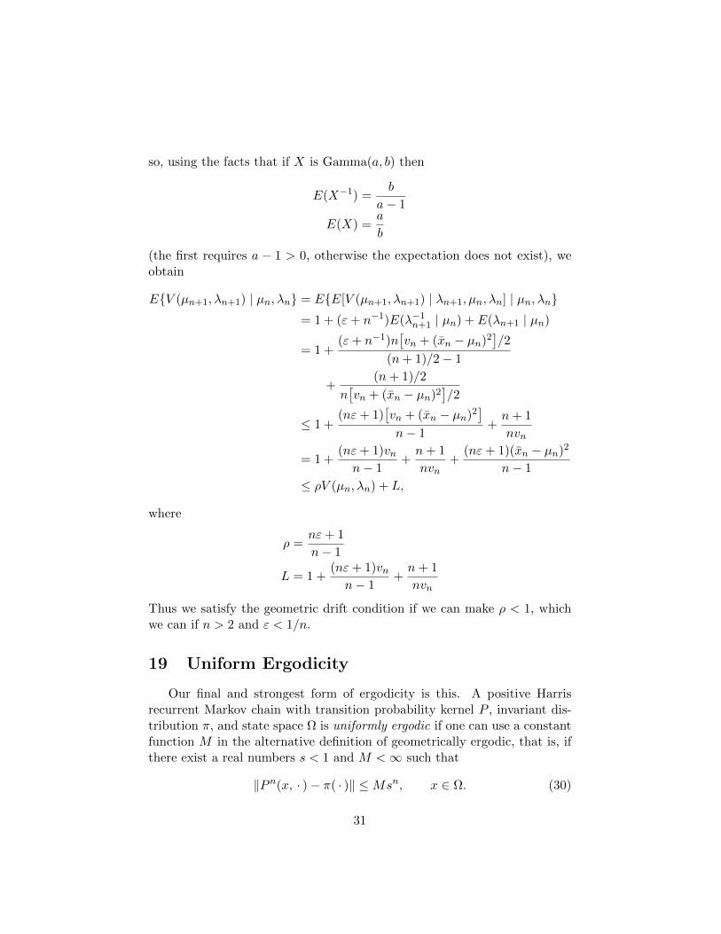
so, using the facts that if X is Gamma(a, b) then

E(X−1) =b

a− 1

E(X) =a

b

(the first requires a − 1 > 0, otherwise the expectation does not exist), weobtain

EV (µn+1, λn+1) | µn, λn = EE[V (µn+1, λn+1) | λn+1, µn, λn] | µn, λn= 1 + (ε+ n−1)E(λ−1

n+1 | µn) + E(λn+1 | µn)

= 1 +(ε+ n−1)n

[vn + (xn − µn)2

]/2

(n+ 1)/2− 1

+(n+ 1)/2

n[vn + (xn − µn)2

]/2

≤ 1 +(nε+ 1)

[vn + (xn − µn)2

]n− 1

+n+ 1

nvn

= 1 +(nε+ 1)vnn− 1

+n+ 1

nvn+

(nε+ 1)(xn − µn)2

n− 1

≤ ρV (µn, λn) + L,

where

ρ =nε+ 1

n− 1

L = 1 +(nε+ 1)vnn− 1

+n+ 1

nvn

Thus we satisfy the geometric drift condition if we can make ρ < 1, whichwe can if n > 2 and ε < 1/n.

19 Uniform Ergodicity

Our final and strongest form of ergodicity is this. A positive Harrisrecurrent Markov chain with transition probability kernel P , invariant dis-tribution π, and state space Ω is uniformly ergodic if one can use a constantfunction M in the alternative definition of geometrically ergodic, that is, ifthere exist a real numbers s < 1 and M <∞ such that

‖Pn(x, · )− π( · )‖ ≤Msn, x ∈ Ω. (30)

31

It is obvious that uniform ergodicity (30) implies geometric ergodicity (27),but the reverse implication does not necessarily hold.

Since uniform ergodicity implies geometric ergodicity, by Theorem 16 thegeometric drift condition (28) holds and the drift function V is unboundedoff petite sets and the function M in the alternate definition of geometricergodicity (27) can be taken proportional to V . But this says V must beboth bounded and unbounded off petite sets, which can happen only if thewhole state space is petite. Actually something stronger is true (Meyn andTweedie, 2009, Theorem 16.0.2).

Theorem 18. A Markov chain is uniformly ergodic if and only if the wholestate space is small.

This shows that most Markov chains are not uniformly ergodic, but hereare a few cases where one does have uniform ergodicity.

• The Markov chain is actually an IID sequence, in which case it isobvious from the definition that the whole state space is a small setbecause P (x,A) = π(A) for all x by independence.

• The Markov chain is a T -chain and the state space is compact.

• The state space is finite. In this case the Markov chain is automaticallya T -chain because every function on a discrete topological space iscontinuous and the state space is automatically compact because everyfinite set of any topological space is compact.

In all of these cases the Markov chain is uniformly ergodic if it is positiveHarris recurrent.

20 Types of Ergodicity and Mixing Coefficients

Mixing coefficients, which were introduced in the handout on stationarystochastic processes are much simplified when the stochastic process is astationary positive Harris recurrent Markov chain (Bradley, 1986, Section 4).Let (Ω,A) be the state space, P the transition probability kernel, π theinvariant probability distribution, and L2(π) the set of all functions f such

32

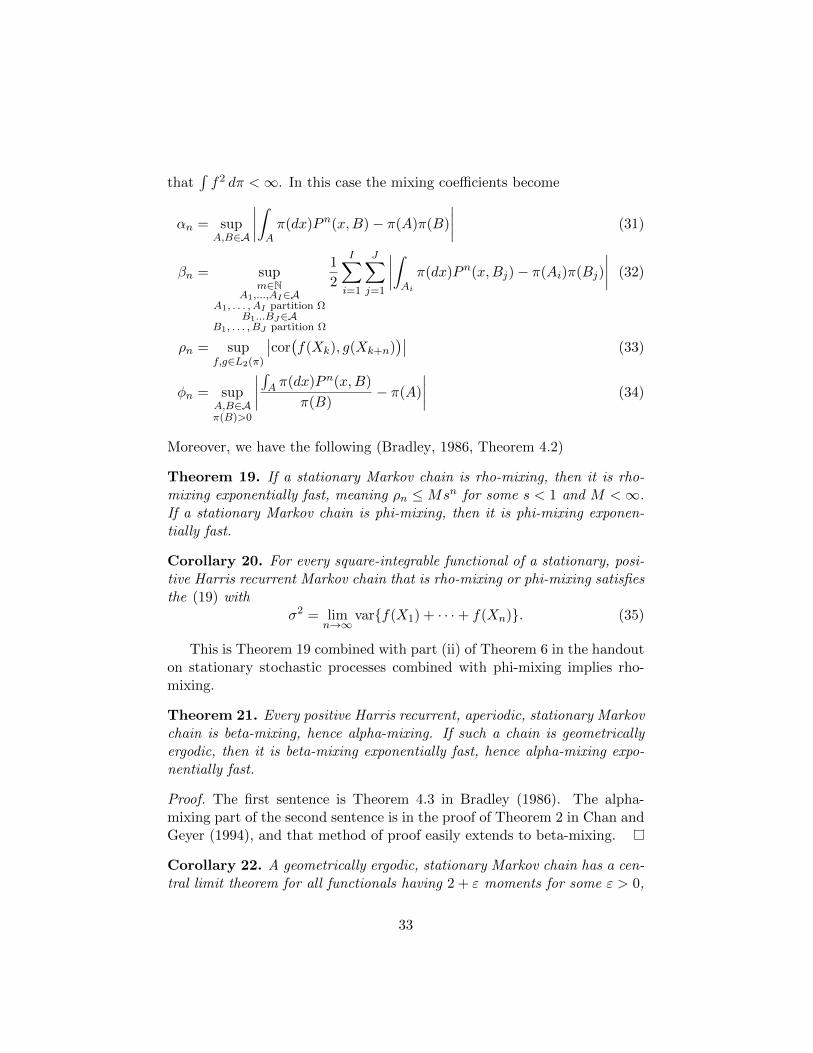
that∫f2 dπ <∞. In this case the mixing coefficients become

αn = supA,B∈A

∣∣∣∣∫Aπ(dx)Pn(x,B)− π(A)π(B)

∣∣∣∣ (31)

βn = supm∈N

A1,...,AI∈AA1, . . . , AI partition Ω

B1...BJ∈AB1, . . . , BJ partition Ω

1

2

I∑i=1

J∑j=1

∣∣∣∣∫Ai

π(dx)Pn(x,Bj)− π(Ai)π(Bj)

∣∣∣∣ (32)

ρn = supf,g∈L2(π)

∣∣cor(f(Xk), g(Xk+n)

)∣∣ (33)

φn = supA,B∈Aπ(B)>0

∣∣∣∣∫A π(dx)Pn(x,B)

π(B)− π(A)

∣∣∣∣ (34)

Moreover, we have the following (Bradley, 1986, Theorem 4.2)

Theorem 19. If a stationary Markov chain is rho-mixing, then it is rho-mixing exponentially fast, meaning ρn ≤Msn for some s < 1 and M <∞.If a stationary Markov chain is phi-mixing, then it is phi-mixing exponen-tially fast.

Corollary 20. For every square-integrable functional of a stationary, posi-tive Harris recurrent Markov chain that is rho-mixing or phi-mixing satisfiesthe (19) with

σ2 = limn→∞

varf(X1) + · · ·+ f(Xn). (35)

This is Theorem 19 combined with part (ii) of Theorem 6 in the handouton stationary stochastic processes combined with phi-mixing implies rho-mixing.

Theorem 21. Every positive Harris recurrent, aperiodic, stationary Markovchain is beta-mixing, hence alpha-mixing. If such a chain is geometricallyergodic, then it is beta-mixing exponentially fast, hence alpha-mixing expo-nentially fast.

Proof. The first sentence is Theorem 4.3 in Bradley (1986). The alpha-mixing part of the second sentence is in the proof of Theorem 2 in Chan andGeyer (1994), and that method of proof easily extends to beta-mixing.

Corollary 22. A geometrically ergodic, stationary Markov chain has a cen-tral limit theorem for all functionals having 2 + ε moments for some ε > 0,

33

that is, (19) holds with

σ2 = varf(Xn)+ 2∞∑k=1

covf(Xn), f(Xn+k) (36)

This is Theorem 21 combined with part (i) of Theorem 5 in the handouton stationary stochastic processes, the formula for σ2 coming from the latter.

For reversible Markov chains (and recall that the Metropolis-Hastingsalgorithm and random-scan Gibbs samplers are reversible) we can do better(Roberts and Rosenthal, 1997, Theorem 2.1).

Theorem 23. Every reversible, geometrically ergodic, stationary Markovchain is rho-mixing.

Corollary 24. A reversible, geometrically ergodic, stationary Markov chainhas a central limit theorem for all square-integrable functionals, that is, (19)holds with σ2 given by (36).

Theorem 25. Every uniformly ergodic, stationary Markov chain is phi-mixing.

Proof. This is shown on pp. 365–366 in Ibragimov and Linnik (1971).

Corollary 26. A uniformly ergodic, stationary Markov chain has a centrallimit theorem for all square-integrable functionals, that is, (19) holds withσ2 given by (35).

Lastly, recall that Theorem 7 says that if the chain is Harris recurrent allof the CLT results hold for any initial distribution, not just for stationarychains.

References

Bradley, R. C. (1986). Basic properties of strong mixing conditions. In Eber-lein, E. and Taqqu, M. S., eds. Dependence in Probability and Statistics:A Survey of Recent Results (Oberwolfach, 1985). Boston: Birkhauser.

Breiman, L. (1968). Probability. Redding, MA: Addison-Wesley. Repub-lished 1992, Philadelphia: Society for Industrial and Applied Mathemat-ics.

Chan, K. S. and Geyer, C. J. (1994). Discussion of Tierney (1994). Annalsof Statistics, 22, 1747–1758.

34

Fristedt, B. E. and Gray, L. F. (1996). A Modern Approach to ProbabilityTheory. Boston: Birkhauser.

Gelfand, A. E. and Smith, A. F. M. (1990). Sampling-based approaches tocalculating marginal densities. Journal of the American Statistical Asso-ciation, 85, 398–409.

Geman, S. and Geman, D. (1984). Stochastic relaxation, Gibbs distribu-tions, and the Bayesian restoration of images. IEEE Transactions onPattern Analysis and Machine Intelligence, 6, 721–741.

Geyer, C. J. (2011). Introduction to Markov chain Monte Carlo. In Handbookof Markov Chain Monte Carlo, edited by Brooks, S., Gelman, A., Jones,G., and Meng, X.-L.. Boca Raton, FL: Chapman & Hall/CRC.

Ibragimov, I. A. and Linnik, Yu. V. (1971). Independent and StationarySequences of Random Variables (edited by J. F. C. Kingman). Groningen:Wolters-Noordhoff.

Hastings, W. K. (1970). Monte Carlo sampling methods using Markov chainsand their applications. Biometrika, 57, 97–109.

Jain, N. and Jamison, B. (1967). Contributions to Doeblin’s theory ofMarkov processes. Zeitschrift fur Wahrscheinlichkeitstheorie und Ver-wandte Gebiete, 8, 19-40.

Metropolis, N., Rosenbluth, A. W., Rosenbluth, M. N., Teller, A. H., andTeller, E. (1953). Equation of state calculations by fast computing ma-chines. Journal of Chemical Physics, 21, 1087–1092.

Meyn, S. P. and Tweedie, R. L. (2009). Markov Chains and StochasticStability, second edition. Cambridge: Cambridge University Press.

Nummelin, E. (1984). General Irreducible Markov Chains and Non-NegativeOperators. Cambridge: Cambridge University Press.

Roberts, G. O. and Rosenthal, J. S. (1997). Electronic Communications inProbability, 2, 13–25.

Rudin, W. (1986). Real and Complex Analysis, third edition. New York:McGraw-Hill.

Tierney, L. (1994). Markov chains for exploring posterior distributions (withdiscussion). Annals of Statistics, 22, 1701–1762.

35