Simulation of SISO and MIMO Multipath Fading...

Antonio Petrolino1 and Gonçalo Tavares2

1Instituto de Engenharia de Sistemas e Computadores - Investigação e Desenvolvimento,INESC-ID, Lisbon

2INESC-ID and Instituto Superior Técnico, IST, LisbonPortugal

1. Introduction

Accurate software simulation is an important step for testing mobile communication systems.It allows the evaluation of the system performance without the need for physical experiments.At an early testing stage, simulations are usually done considering transmissions overadditive white Gaussian noise (AWGN) channels, which do not account for obstacles ormotion between the transmitter (Tx) and the receiver (Rx). According to the AWGN channelmodel, only the thermal noise which comes from the receiver amplifiers and from manynatural sources is considered and added to the transmitted signal. This means that thereceived signal is a copy of the transmitted signal embedded in Gaussian noise, whoseintensity depends on the propagation scenario (including the amplifiers of the Tx and theRx) and can be controlled in simulation by tuning the Gaussian process variance.It is easy to understand that AWGN channel models do not capture the conditions of a realradio channel where the presence of obstacles between the Tx and the Rx causes multipathpropagation and may lead to frequency selective channels. In this situation, several replicasof the transmitted signal get to the Rx antenna with different propagation delays. If thesedelays are not negligible compared to the transmission interval Ts, the attenuation causedby the channel in the frequency-domain is not constant and a distortion is introduced1.Moreover, if there is motion between the Tx and the Rx, the received signal may be affectedby a time-domain multiplicative distortion called fading. This happens because, being theRx in motion relative to the Tx, the propagation channel characteristics vary with time andtheir effect can be modeled as a time-domain distortion affecting the transmitted signal. Bycombining both the effects of multipath propagation and fading on a wireless transmission,the received signal baseband equivalent r(t) may be expressed as

r(t) =N(t)

∑i=1

ρi(t)ejθi(t)s(t − τi(t)) + n(t) (1)

where s(t) is the transmitted signal baseband equivalent, ρi(t) and θi(t) are the time-varyingattenuation and phase shift respectively of the i-th path and n(t) is a white Gaussian process

1 Otherwise, when the propagation delays are negligible compared to the signal interval, the channel issaid to be flat.

Simulation of SISO and MIMO Multipath Fading Channels

2

www.intechopen.com

modeling thermal noise and noise added by the receiver amplifiers. Although in the case oftime varying channels N(t) and τi(t) are functions of the time, for the sake of simplicity, it iscommon in the literature to ignore the dependence on time of the number of significant pathsand the propagation delays, that is to set N(t) = N and τi(t) = τi. Eq. (1) can be rewritten as

r(t) =N

∑i=1

ρi(t)ejθi(t)s(t − τi) + n(t)

=N

∑i=1

hi(t)s(t − τi) + n(t)

(2)

where hi(t) � ρi(t)ejθi(t). Eq. (2) represents the received signal in the case of transmission overa frequency-selective channel.In the case of flat multipath channels a further simplification is possible since τi ≅ τ ≪ Ts ∀i.Eq. (2) can be rewritten as

r(t) =N

∑i=1

hi(t) · s(t − τ) + n(t). (3)

Moreover, if a large number of paths is considered i.e., N ≫ 1, the central limit theorem canbe applied to the sum in (3) leading to

r(t) = h(t) · s(t − τ) + n(t) (4)

where h(t) = hR(t) + jhI(t) is a complex Gaussian random process.By comparing equations (2) and (4), it is clear that the selectivity in the frequency-domainrequires the contribution of each path to be considered and that the fading process, being thecombination of N complex processes, each modeling the fading affecting the correspondingpropagation path, can not be approximated by a Gaussian random process.As far as flat fading channels are concerned, a detailed description of the process h(t)was derived by Clarke in 1968. According to the model of Clarke (Clarke, 1968), for amobile-to-fixed channel, the fading quadrature components are independent each with thesame autocorrelation function (ACF) given by (Pätzold, 2002)

RhR(τ) = RhI

(τ) = Rh(τ) =σ2

h

2· J0(2π fDτ) (5)

where σ2h is the fading power, J0(·) is the zero-order Bessel function of the first kind and fD is

the maximum Doppler frequency shift. Two other widely used statistics in channel modelingfor the statistical characterization of a fading process are the level crossing rate (LCR) and theaverage fade duration (AFD) of the process. The LCR LR is defined as the expected number oftimes per second that the envelope |h(t)| crosses the threshold R in the positive direction. ForRayleigh fading, it is given as (Patel et al., 2005)

LR =√

2π fDρe−ρ2, (6)

where ρ = R/√

E[|h(t)|2] (here, E[·] denotes expectation). The AFD TR is defined as theexpected value for the length of the time intervals in which the stochastic process h(t) is belowa given level R. For Rayleigh fading, it is given as (Patel et al., 2005)

TR =eρ2 − 1√2π fDρ

. (7)

12 Vehicular Technologies: Increasing Connectivity

www.intechopen.com

It is important to note that some characteristics of the fading process, like the amplitudeprobability density function (PDF), can change considerably depending on the propagationscenario. For example, when a line-of-sight path is not available it can be shown thatthe complex Gaussian process h(t) in (4) has zero-mean. Consequently, the fading processenvelope PDF follows a Rayleigh distribution. Otherwise, when a line-of-sight path isavailable, the Gaussian process h(t) has non-zero-mean leading to a Rician distributedenvelope. However, experience shows that often the hypotheses of the model of Clarke arenot verified and the fading severity turns out to be different from Rayleigh or Rician. Insuch cases, distributions like Nakagami-m (Nakagami, 1960), Weibull (Weibull, 1951) or Hoyt(Hoyt, 1947) match more closely with real fadings (Vehicular Technology Society Committeeon Radio Propagation, 1988).Simulation of fading processes with Rayleigh and Rician fading envelopes has beenextensively studied e.g., the sum-of-sinusoids (SoS) method proposed in (Jakes, 1974), thesimulator based on the inverse fast Fourier Transform (IFFT) proposed in (Smith, 1975),the filtering method presented in (Komninakis, 2003) and the simulator based on theKarhunen-Loève (KL) expansion presented in (Petrolino et al., 2008a).The first approach, proposed by Jakes in (Jakes, 1974) is limited to the simulation of theClarke’s model for which it has been developed. It is based on the representation of thereceived signal as a superposition of a finite number of sinusoids having equal amplitudeand uniformly spaced angle of arrivals. Jakes’ simulator has to be considered as deterministic(Pätzold et al., 1998), since the generated waves depend on parameters which, once chosen,remain fixed for the duration of the simulation run. The SoS method was improved in (Pop &Beaulieu, 2001), with the addition of random phases, with the goal of making the generatedprocess wide sense stationary (WSS).The second approach, named IFFT-based method, was proposed in (Smith, 1975) andextended in (Young & Beaulieu, 2000). With this method, in order to achieve a fading outputwith the desired ACF, two real sequences of zero-mean independent Gaussian randomvariables (rvs) are multiplied in the frequency-domain by the same frequency mask equal tothe square root of the power spectral density (PSD) corresponding to the desired ACF. Then,the obtained sequences are added in quadrature and a complex IFFT is taken. Due to thelinearity of the IFFT, the output is a time-domain Gaussian sequence with the desired ACF.The third approach is known as filtering method and resorts to digital filtering ofcomputer-generated independent Gaussian rvs by a filter whose magnitude frequencyresponse is given by the square root of the desired PSD. Due to the linearity of the filteringoperation, the filter output sequence is still Gaussian and has the desired ACF. A solutionbased on the combination of an infinite impulse response (IIR) filter with a nearly idealinterpolator is proposed in (Komninakis, 2003).The last approach is based on the idea of expanding the complex random fading process as amodified KL expansion. Let h(t) be a correlated zero-mean complex Gaussian random processin 0 < t < T0 whose quadrature components are independent each showing the same ACF.The process h(t) can be represented by the series expansion (Van Trees, 1968)

h(t) = limL→∞

L−1

∑l=0

hlφl(t) (8)

where the set of functions {φl(t)}L−1l=0 is the basis of the expansion and the {hl}L−1

l=0 arethe expansion coefficients, that is the projections of the process h(t) on the basis functions.The representation in (8) is known as the Karhunen-Loève expansion for the process h(t)

13Simulation of SISO and MIMO Multipath Fading Channels

www.intechopen.com

(Van Trees, 1968). Since h(t) is a zero-mean complex Gaussian random process and the

{φl(t)}L−1l=0 are orthogonal, the {hl}L−1

l=0 are zero-mean, independent complex Gaussian rvs

with variances {σ2l }L−1

l=0 . A possible expansion for the process h(t) is achieved by setting the

process h(t) correlation matrix eigenvectors and eigenvalues as the basis functions {φl(t)}L−1l=0

and the variances {σ2l }L−1

l=0 , respectively (Petrolino et al., 2008b). Inversely, in fading channelsimulation we need to generate a correlated random process starting from the a prioriknowledge of its ACF which is determined by the channel model being used. This can be

achieved by following the approach proposed in (Petrolino et al., 2008a), where the {φl(t)}L−1l=0

is imposed as a complete set of exponential functions, leading to a modified KL expansion.Due to the particular choice of the basis functions, the eigenvalues can be calculated forl = 0, . . . , L − 1, as (Petrolino et al., 2008b, eq. (9))

σ2l =

∫ T0/2

−T0/2Rh(τ) cos

(2πlτ

T0

)

dτ. (9)

This means that if we are able to calculate the integral in (9) for every l, then the processh(t) may be synthesized by (8) using a set of L computer-generated independent zero-mean

Gaussian rvs, with variances {σ2l }

L−1l=0 .

At this point a N-samples version h[n] of the fading process h(t) may be obtained by samplingthe interval T0 with sampling frequency fs = N/T0

h[n] =L−1

∑l=0

hl · ej 2πN ln n = 0, . . . , N − 1 (10)

where the {hl}L−1l=0 ∼ N(0, {σ2

l }L−1l=0 ) are independent Gaussian rvs. The dimension of the

expansion basis is (Van Trees, 1968) L = 2BT0 where B is the unilateral bandwidth of theprocess and T0 its duration. Since T0 = NTs, the KL expansion dimension reduces to L =2BNTs = 2B

fsN ≤ N, where the inequality follows from the sampling theorem. This means

that hl = 0 for l ≥ N, so it is possible to rewrite (10) as

h[n] =N−1

∑l=0

hl · ej 2πN ln n = 0, . . . , N − 1 (11)

that is, h[n] is the IDFT of the sequence {hl}N−1l=0 and may be computed efficiently using

the fast Fourier transform (FFT) algorithm. Note that simulators like (Young & Beaulieu,2000), (Komninakis, 2003) and (Petrolino et al., 2008a) impose the desired ACF by lineartransformations of Gaussian processes. By the properties of this class of processes, theGaussian PDF is preserved. However, this is not the case with non-Gaussian processes.As a consequence, such simulators can not be directly used to generate autocorrelatednon-Gaussian sequences like Nakagami-m, Weibull or Hoyt. Regarding Nakagami-m fading,simulators have been proposed in (Beaulieu & Cheng, 2001) and (Filho et al., 2007), both ofwhich require already-correlated Rayleigh sequences which must be generated by existingsimulators. In (Beaulieu & Cheng, 2001), the correlated Nakagami sequence is obtained byapplying a double transformation to the Rayleigh sequence, while in (Filho et al., 2007), anuncorrelated Nakagami sequence is rearranged according to the Rayleigh sequence rankingin order to match the desired ACF.


www.intechopen.com

An important class of systems which have gained success in the last years are multiple-inputmultiple-output (MIMO) systems. Consequently, MIMO fading channel simulators areincreasingly required by MIMO designers for system performance evaluation and assessment.In MIMO systems, multi-element antenna arrays are used at both sides of a radio link andthe communication occurs over Nmin parallel channels, where Nmin is the minimum of thenumber of Tx or Rx antennas (Gesbert et al., 2000). Due to finite antenna separation, a spatialcorrelation between the channels always exists and greatly affects the link capacity of MIMOsystems (Wang, 2006). The MIMO channel spatial correlation can be described by a MN×MNcorrelation matrix. This matrix can be obtained in several ways depending on the referencemodel under consideration. In this chapter we will use the Kronecker Based Stochastic Model(KBSM) (Wang, 2006). According to the KBSM model, the spatial correlation matrix SMI MO isobtained as

SMI MO = SBS ⊗ SMS (12)

where SBS is the M×M spatial correlation matrix at the BS, SMS is the N×N spatial correlationmatrix at the MS and ⊗ stands for the Kronecker product. For the referred reasons, a MIMOfading channel simulator must contemplate the possibility of generating random processescross-correlated according to a spatial correlation structure determined by the used model.In general, the fading channel simulation can be divided in three tasks:

1. Choice of the most convenient fading channel model.

2. Generation of uncorrelated rvs with the desired PDF. This point will be discussed inSections 2 and 3.

3. Imposition of the desired ACF to the generated sequence without affecting the initial PDF.This point will be analyzed in Section 4.

This chapter is organized as follows. Section 2 presents a technique for the generationof uncorrelated arbitrary jointly distributed phase and envelope processes. The proposedmethod is based on the two-dimensional extension of the Metropolis-Hastings (MH)algorithm (Hastings, 1970; Metropolis et al., 1953). Starting from jointly Gaussian randomvariate pairs, this method achieves the desired PDF by an acceptance-rejection (AR) algorithmwhose probability of acceptance is set in a convenient way.In Section 3, the two-dimensional MH algorithm is applied to the generation of Nakagami-mand Hoyt envelope fading processes.Section 4 presents a method for inducing the desired correlation structure on wireless channelsimulation processes. It will be shown that it can be used for simulating both the spatialcorrelation between the propagation channels for MIMO systems and the time-ACF in case ofsingle-input single-output (SISO) systems. The procedure is based on the method proposed byIman & Conover (IC) in 1982 (Iman & Conover, 1982). This method is able to induce a desiredcorrelation matrix on an input matrix whose columns are random vectors with independentarbitrary marginal distributions (Petrolino & Tavares, 2010a), (Petrolino & Tavares, 2010b).The IC method is distribution-free, which means that it preserves the marginal PDF of theinput sequences while inducing the desired correlation. This important feature enables thegeneration of sequences with arbitrarily distributed PDFs and arbitrary correlation matrix.Section 5 presents simulation results obtained by applying the IC method to the simulationof MIMO and SISO channels. In the MIMO case the simulated spatial correlation matrices arecompared with the targets, while in the SISO case the comparison is made between the targetand the simulated time ACFs. In both cases, perfect preservation of the initial PDF is achieved.Finally, Section 6 concludes the chapter.


www.intechopen.com

2. The Metropolis-Hastings algorithm

In this Section, we present a computational efficient and accurate method for simulating everytype of fading (e.g. Nakagami-m, Weibull, Hoyt, etc.) starting from PDFs (e.g. Gaussian orUniform distribution) which can be easily generated by known and efficient methods. Thismethod is based on the Metropolis-Hastings algorithm (Hastings, 1970; Metropolis et al., 1953)with an AR sampling proposed by Tierney in (Tierney, 1994).Consider now the problem of simulating a fading channel characterized by arbitrary jointlydistributed envelope and phase. For this purpose, let h(t) = x(t) + jy(t) be a complex fading

process and let h(t) = ρ(t)ejθ(t) be its representation in polar coordinates.Two possible ways exist for generating h(t): the first is the direct generation of the envelopeand phase processes ρ(t) and θ(t) respectively, the second is generating the IQ componentprocesses x(t) and y(t). The first solution is attractive in the sense that the characterizationof fading channels is usually done in terms of envelope and phase PDFs. However, intelecommunications, system testing is usually carried out by considering the transmissionof the signal IQ components over the fading channel under consideration.Recalling that the IQ components joint PDF fXY(x, y) and the phase-envelope joint PDFfR,θ(ρ, θ) are related by

fXY(x, y) =fR,Θ(ρ, θ)

|J| (13)

where |J| is the Jacobian of the transformation

x = ρ cos θ, y = ρ sin θ (14)

we conclude that if we are able to generate pairs of rvs (xi, yi) following the joint PDF fXY(x, y)in (13), then the phase-amplitude joint PDF will be the desired fR,Θ(ρ, θ). The main issue insimulating fading processes is that usually, the distribution fXY(x, y) does not belong to anyfamily of well-known PDFs and can not be directly generated. Here, we propose a methodwhich allows the efficient generation of rvs with arbitrary distribution.

Suppose we want to generate a set of N pairs (x(i)1 , x

(i)2 )|i=1,...,N following an arbitrary target

joint density f (·) whose analytical expression is known, and that we have pairs (y1, y2) froma candidate-generating joint density h(·) that can be simulated by some known, inexpensive

method. After setting an arbitrary initial pair (x(0)1 , x

(0)2 ) for initializing the algorithm, the

MH method can be summarized as follows (Chib & Greenberg, 1995):

• Repeat the following steps for i = 0, . . . , N − 1

• Generate (y1, y2) from h(·) and u from a uniform distribution u ∼ U (0, 1)

• IF u ≤ α

Set (x(i+1)1 , x

(i+1)2 ) = (y1, y2)

• ELSE

Set (x(i+1)1 , x

(i+1)2 ) = (x

(i)1 , x

(i)2 )

where α = α[(x(n)1 , x

(n)2 ), (y1, y2)] is the (conditional) probability of accepting the candidate

pair (y1, y2) given that the current pair is (x(n)1 , x

(n)2 ). This probability is usually called

probability of move (Chib & Greenberg, 1995), because it represents the probability of the process


www.intechopen.com

moving to a new state. When the MH algorithm was proposed, this probability was set to(Tierney, 1994)

α = min

{

f (y1, y2)

f (x(i)1 , x

(i)2 )

, 1

}

(15)

which means that the higher is the target PDF at the candidate pair, the higher is theprobability to accept it. Here we use a modified version of the MH algorithm.This modification has been discussed in (Tierney, 1994) and it is based on the idea ofintroducing an acceptance-rejection step for generating candidates for a MH algorithm.Pairs (y1, y2) are generated from Kh(·) until a pair satisfying u < f (y1, y2), where u ∼U{0, Kh(y1, y2)}, in obtained. The constant K is set such that f (x1, x2) ≤ Kh(x1, x2) for all(x1, x2) and controls the acceptance rate. According to this method, only those pairs for whichthe target density f (·) is high are accepted as candidates for the MH algorithm. Moreover, theprobability of move α is set as follows. Let

C = {(a, b) : f (a, b) < Kh(a, b)} (16)

be the set where Kh(a, b) dominates f (a, b). Four possible cases occur and the probability α isset as follows (Chib & Greenberg, 1995):

• Case (a): (x(n)1 , x

(n)2 ) ∈ C and (y1, y2) ∈ C.

In this case Kh(·) dominates f (·) for both the current and the candidate pair. This meansthat with higher probability both pairs belong to Kh(·) rather than to the target PDF f (·).In this case the algorithm always accepts the new pair i.e., α = 1;

• Case (b): (x(n)1 , x

(n)2 ) ∈ C and (y1, y2) /∈ C.

In this case the current pair belongs with higher probability to Kh(·) rather than to f (·).Moreover, for the candidate pair, f (·) is higher than Kh(·). This means that the probabilityof belonging to the target density is higher for the candidate pair than for the current pair.Also in this case the algorithm always accepts the new one i.e., α = 1;

• Case (c): (x(n)1 , x

(n)2 ) /∈ C and (y1, y2) ∈ C.

The probability of belonging to f (·) is higher for the current pair than for the candidatepair. This means that the transition to other states must be controlled. In this case themethods sets

α =Kh(x

(n)1 , x

(n)2 )

f (x(n)1 , x

(n)2 )

.

Note that the higher the value of the target density f (·) at the current pair, the lower theprobability to accept the candidate pair;

• Case (d): (x(n)1 , x

(n)2 ) /∈ C and (y1, y2) /∈ C.

Both the current and the candidate pair belong with higher probability to the target PDFf (·) rather than to the candidate Kh(·). Also in this case the probability of move dependson the target and the candidate densities. It is easy to understand that it must be set suchit is in general higher than in the previous case. The method in this case sets

α = min

{

f (y1, y2) · h(x(n)1 , x

(n)2 )

f (x(n)1 , x

(n)2 ) · h(y1, y2)

, 1

}

.

Note that the higher the product f (x(n)1 , x

(n)2 ) · h(y1, y2), the lower the probability of move.


www.intechopen.com

Compared with the standard MH algorithm, this version of the algorithm provides a PDFwith a better match with the target distribution. This is achieved by observing that theinitial distribution support can be divided in two kind of zones, one producing good valueswith higher probability than the other. It is important to note that, contrary to the standardMH algorithm, this method will occasionally reject candidates if the process is at a pair

(x(n)1 , x

(n)2 ) /∈ C (Tierney, 1994). By keeping the same pair for a certain number of consecutive

steps, Metropolis-based methods introduce in general correlation along the sampled series.This can be harmful if uncorrelated processes are required. Our goal in this paper is togenerate uncorrelated fading processes with desired envelope and phase PDFs. In this way,distribution-free algorithms can be applied to the generated pairs for imposing the desiredcorrelation if second order statistics specification is required. We got round this difficulty byapplying a random shuffling to the generated sequence at the end of the algorithm.

3. Simulation of uncorrelated arbitrary jointly distributed phase and envelope

processes with the MH algorithm

In this Section we will show some results obtained by applying the previously described MHalgorithm to two different propagation scenarios. We simulated the IQ components of fadingchannels characterized by arbitrarily distributed envelope and phase processes. As requiredby the algorithm we deduced analytical expressions of the target IQ components joint PDFf (·) from results available in the literature. In both the following examples the candidatepairs (y1, y2) follow the bivariate joint Gaussian PDF. They are independent Gaussian rvswith zero-mean and the same variance σ2, so that their joint PDF reduces to the product oftheir Gaussian marginal PDFs and is given by

h(y1, y2) =1

2πσ2exp

(

− y21 + y2

2

2σ2

)

. (17)

The constant K introduced in equation (16) has been adjusted by experimentation to achievean acceptance rate of about 50%.A rv representing a realization of a fading process at a fixed instant of time is

C = X + jY (18)

where X and Y are rvs representing the fading process IQ components and

R =√

X2 + Y2 Θ = tan−1(Y/X) (19)

are the envelope and the phase of C respectively. From (14), since the Jacobian is |J| = ρ, wehave that

fXY(x, y) =fR,Θ(ρ, θ)

ρ. (20)

3.1 Nakagami-m fading

For Nakagami-m fading, the envelope PDF is given by the well-known formula (Nakagami,1960)

fR(ρ) =2mmρ2m−1

ΩmΓ(m)exp

(

−mρ2

Ω

)

, ρ ≥ 0 m >1

2(21)


www.intechopen.com

where Ω = E[R2] is the mean power, m = Ω2/V[R2] is the Nakagami fading parameter (V[·]denotes variance) and Γ(·) is the Gamma function.For independent I and Q components, the corresponding phase PDF has been obtained in(Yacoub et al., 2005) and is given by

fΘ(θ) =Γ(m)| sin(2θ)|m−1

2mΓ2(m/2), −π ≤ θ < π. (22)

Considering the envelope and the phase as independent rvs, we have

fR,Θ(ρ, θ) = fR(ρ) × fΘ(θ). (23)

The substitution of (23) into (20) leads to

fXY(x, y) =mm| sin(2θ)|m−1ρ2m−2

2m−1ΩmΓ2(m/2)exp

(

−mρ2

Ω

)

(24)

where ρ =√

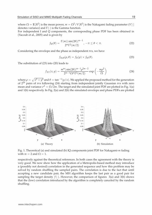
x2 + y2 and θ = tan−1(y/x). We applied the proposed method for the generationof 220 pairs of rvs following (24) starting from independent jointly Gaussian rvs with zeromean and variance σ2 = Ω/2m. The target and the simulated joint PDF are plotted in Fig. 1(a)and 1(b) respectively. In Fig. 2(a) and 2(b) the simulated envelope and phase PDFs are plotted

−5

0

5

−5

0

50

0.05

0.1

0.15

0.2

0.25

0.3

0.35

0.4

xy

f XY(x

,y)

(a) Theory

−5

0

5

−5

0

50

0.05

0.1

0.15

0.2

0.25

0.3

0.35

0.4

xy

f XY(x

,y)

(b) Simulation

Fig. 1. Theoretical (a) and simulated (b) IQ components joint PDF for Nakagami-m fadingwith m = 2 and Ω = 1.

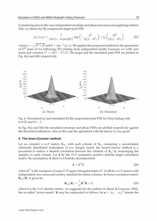
respectively against the theoretical references. In both cases the agreement with the theory isvery good. We now show how the application of a Metropolis-based method may introducea (possibly not desired) correlation in the generated sequence and how this problem may besolved by random shuffling the sampled pairs. The correlation is due to the fact that untilaccepting a new candidate pair, the MH algorithm keeps the last pair as a good pair forsampling the target density f (·). However, the comparison of figures 3(a) and 3(b) showsthat the (low) correlation introduced by the algorithm is completely canceled by the randomshuffling.


www.intechopen.com

0 0.5 1 1.5 2 2.5 30

0.2

0.4

0.6

0.8

1

1.2

1.4

ρ

f R(ρ

)

Theory

Simulation

(a) Envelope PDF

−4 −3 −2 −1 0 1 2 3 40

0.05

0.1

0.15

0.2

0.25

0.3

0.35

θ

f Θ(θ

)

Theory

Simulation

(b) Phase PDF

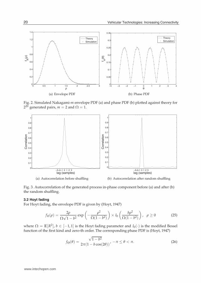
Fig. 2. Simulated Nakagami-m envelope PDF (a) and phase PDF (b) plotted against theory for220 generated pairs, m = 2 and Ω = 1.

0−1 1−2−3 2 30

0.1

0.2

0.3

0.4

0.5

0.6

0.7

0.8

0.9

1

lag (samples)

Co

rre

latio

n

(a) Autocorrelation before shuffling

0−1 1−2−3 2 3

0

0.1

0.2

0.3

0.4

0.5

0.6

0.7

0.8

0.9

1

lag (samples)

Co

rre

latio

n

(b) Autocorrelation after random shuffling

Fig. 3. Autocorrelation of the generated process in-phase component before (a) and after (b)the random shuffling.

3.2 Hoyt fading

For Hoyt fading, the envelope PDF is given by (Hoyt, 1947)

fR(ρ) =2ρ

Ω√

1 − b2exp

(

− ρ2

Ω(1 − b2)

)

× I0

(bρ2

Ω(1 − b2)

)

, ρ ≥ 0 (25)

where Ω = E[R2], b ∈ [−1, 1] is the Hoyt fading parameter and I0(·) is the modified Besselfunction of the first kind and zero-th order. The corresponding phase PDF is (Hoyt, 1947)

fΘ(θ) =

√1 − b2

2π(1 − b cos(2θ)), −π ≤ θ < π. (26)


www.intechopen.com

Considering also in this case independent envelope and phase processes and applying relation(20), we obtain the IQ components target joint PDF

fXY(x, y) =1

Ωπ(1 − b cos(2θ))exp

(

− ρ2

Ω(1 − b2)

)

× I0

(bρ2

Ω(1 − b2)

)

(27)

where ρ =√

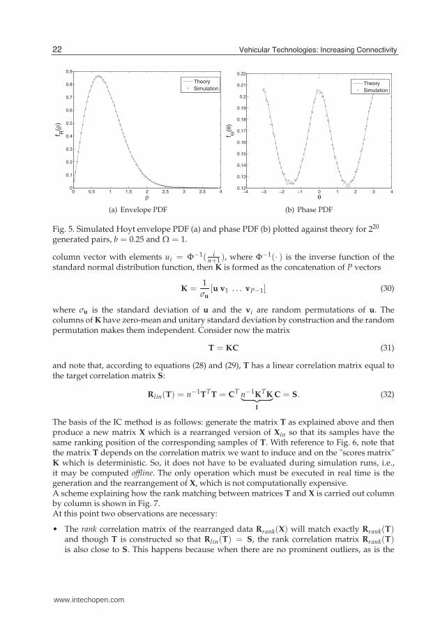
x2 + y2 and θ = tan−1(y/x). We applied the proposed method for the generationof 220 pairs of rvs following (27) starting from independent jointly Gaussian rvs with zeromean and variance σ2 = Ω(1 − b2)/2. The target and the simulated joint PDF are plotted inFig. 4(a) and 4(b) respectively.

−5

0

5 −5

0

50

0.05

0.1

0.15

0.2

0.25

0.3

0.35

0.4

0.45

0.5

xy

f XY(x

,y)

(a) Theory

−5

0

5

−5

0

50

0.05

0.1

0.15

0.2

0.25

0.3

0.35

0.4

0.45

0.5

xy

f XY(x

,y)

(b) Simulation

Fig. 4. Theoretical (a) and simulated (b) IQ components joint PDF for Hoyt fading withb=0.25 and Ω = 1.

In Fig. 5(a) and 5(b) the simulated envelope and phase PDFs are plotted respectively againstthe theoretical references. Also in this case the agreement with the theory is very good.

4. The Iman-Conover method

Let us consider a n×P matrix Xin, with each column of Xin containing n uncorrelatedarbitrarily distributed realizations of rvs. Simply stated, the Iman-Conover method is aprocedure to induce a desired correlation between the columns of Xin by rearranging thesamples in each column. Let S be the P×P symmetric positive definite target correlationmatrix. By assumption, S allows a Cholesky decomposition

S = CT

C (28)

where CT is the transpose of some P×P upper triangular matrix C. Let K be a n×P matrix with

independent, zero-mean and unitary standard deviation columns. Its linear correlation matrixRlin(K) is given by

Rlin(K) =1

nK

TK = I (29)

where I is the P×P identity matrix. As suggested by the authors in (Iman & Conover, 1982),the so-called "scores matrix" K may be constructed as follows: let u = [u1 . . . un]T denote the


www.intechopen.com

0 0.5 1 1.5 2 2.5 3 3.5 40

0.1

0.2

0.3

0.4

0.5

0.6

0.7

0.8

0.9

ρ

f R(ρ

)

Theory

Simulation

(a) Envelope PDF

−4 −3 −2 −1 0 1 2 3 40.12

0.13

0.14

0.15

0.16

0.17

0.18

0.19

0.2

0.21

0.22

θ

f Θ(θ

)

Theory

Simulation

(b) Phase PDF

Fig. 5. Simulated Hoyt envelope PDF (a) and phase PDF (b) plotted against theory for 220

generated pairs, b = 0.25 and Ω = 1.

column vector with elements ui = Φ−1( in+1 ), where Φ−1(· ) is the inverse function of the

standard normal distribution function, then K is formed as the concatenation of P vectors

K =1

σu

[u v1 . . . vP−1] (30)

where σu is the standard deviation of u and the vi are random permutations of u. Thecolumns of K have zero-mean and unitary standard deviation by construction and the randompermutation makes them independent. Consider now the matrix

T = KC (31)

and note that, according to equations (28) and (29), T has a linear correlation matrix equal tothe target correlation matrix S:

Rlin(T) = n−1T

TT = C

T n−1K

TK

︸︷︷︸

I

C = S. (32)

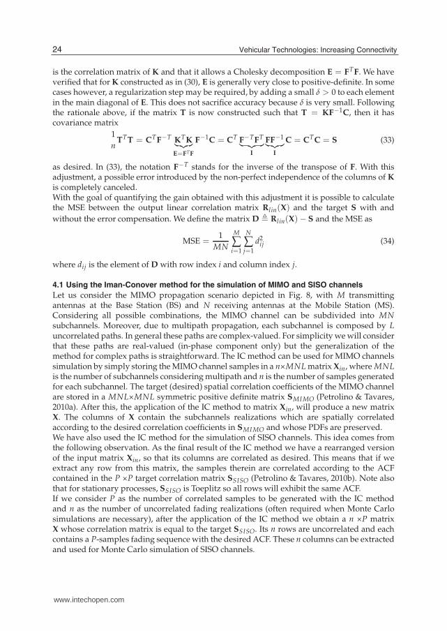
The basis of the IC method is as follows: generate the matrix T as explained above and thenproduce a new matrix X which is a rearranged version of Xin so that its samples have thesame ranking position of the corresponding samples of T. With reference to Fig. 6, note thatthe matrix T depends on the correlation matrix we want to induce and on the "scores matrix"K which is deterministic. So, it does not have to be evaluated during simulation runs, i.e.,it may be computed offline. The only operation which must be executed in real time is thegeneration and the rearrangement of X, which is not computationally expensive.A scheme explaining how the rank matching between matrices T and X is carried out columnby column is shown in Fig. 7.At this point two observations are necessary:

• The rank correlation matrix of the rearranged data Rrank(X) will match exactly Rrank(T)and though T is constructed so that Rlin(T) = S, the rank correlation matrix Rrank(T)is also close to S. This happens because when there are no prominent outliers, as is the


www.intechopen.com

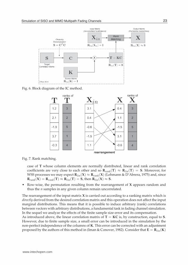
Fig. 6. Block diagram of the IC method.

Fig. 7. Rank matching.

case of T whose column elements are normally distributed, linear and rank correlationcoefficients are very close to each other and so Rrank(T) ≈ Rlin(T) = S. Moreover, forWSS processes we may expect Rlin(X) ≈ Rrank(X) (Lehmann & D’Abrera, 1975) and, sinceRrank(X) = Rrank(T) ≈ Rlin(T) = S, then Rlin(X) ≈ S.

• Row-wise, the permutation resulting from the rearrangement of X appears random andthus the n samples in any given column remain uncorrelated.

The rearrangement of the input matrix X is carried out according to a ranking matrix which isdirectly derived from the desired correlation matrix and this operation does not affect the inputmarginal distributions. This means that it is possible to induce arbitrary (rank) correlationsbetween vectors with arbitrary distributions, a fundamental task in fading channel simulation.In the sequel we analyze the effects of the finite sample size error and its compensation.As introduced above, the linear correlation matrix of T = KC is, by construction, equal to S.However, due to finite sample size, a small error can be introduced in the simulation by thenon-perfect independence of the columns of K. This error can be corrected with an adjustmentproposed by the authors of this method in (Iman & Conover, 1982). Consider that E = Rlin(K)


www.intechopen.com

is the correlation matrix of K and that it allows a Cholesky decomposition E = FT

F. We haveverified that for K constructed as in (30), E is generally very close to positive-definite. In somecases however, a regularization step may be required, by adding a small δ > 0 to each elementin the main diagonal of E. This does not sacrifice accuracy because δ is very small. Followingthe rationale above, if the matrix T is now constructed such that T = KF

−1C, then it has

covariance matrix

1

nT

TT = C

TF−T

KT

K︸︷︷︸

E=FTF

F−1

C = CT

F−T

FT

︸︷︷︸

I

FF−1

︸︷︷︸

I

C = CT

C = S (33)

as desired. In (33), the notation F−T stands for the inverse of the transpose of F. With this

adjustment, a possible error introduced by the non-perfect independence of the columns of K

is completely canceled.With the goal of quantifying the gain obtained with this adjustment it is possible to calculatethe MSE between the output linear correlation matrix Rlin(X) and the target S with and

without the error compensation. We define the matrix D � Rlin(X) − S and the MSE as

MSE =1

MN

M

∑i=1

N

∑j=1

d2ij (34)

where dij is the element of D with row index i and column index j.

4.1 Using the Iman-Conover method for the simulation of MIMO and SISO channels

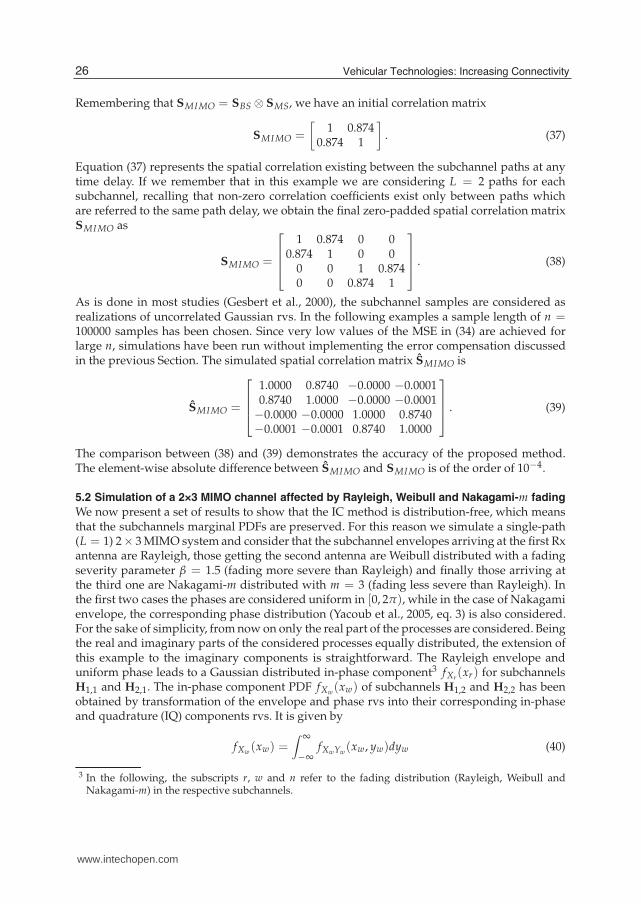
Let us consider the MIMO propagation scenario depicted in Fig. 8, with M transmittingantennas at the Base Station (BS) and N receiving antennas at the Mobile Station (MS).Considering all possible combinations, the MIMO channel can be subdivided into MNsubchannels. Moreover, due to multipath propagation, each subchannel is composed by Luncorrelated paths. In general these paths are complex-valued. For simplicity we will considerthat these paths are real-valued (in-phase component only) but the generalization of themethod for complex paths is straightforward. The IC method can be used for MIMO channelssimulation by simply storing the MIMO channel samples in a n×MNL matrix Xin, where MNLis the number of subchannels considering multipath and n is the number of samples generatedfor each subchannel. The target (desired) spatial correlation coefficients of the MIMO channelare stored in a MNL×MNL symmetric positive definite matrix SMI MO (Petrolino & Tavares,2010a). After this, the application of the IC method to matrix Xin, will produce a new matrixX. The columns of X contain the subchannels realizations which are spatially correlatedaccording to the desired correlation coefficients in SMI MO and whose PDFs are preserved.We have also used the IC method for the simulation of SISO channels. This idea comes fromthe following observation. As the final result of the IC method we have a rearranged versionof the input matrix Xin, so that its columns are correlated as desired. This means that if weextract any row from this matrix, the samples therein are correlated according to the ACFcontained in the P ×P target correlation matrix SSISO (Petrolino & Tavares, 2010b). Note alsothat for stationary processes, SSISO is Toeplitz so all rows will exhibit the same ACF.If we consider P as the number of correlated samples to be generated with the IC methodand n as the number of uncorrelated fading realizations (often required when Monte Carlosimulations are necessary), after the application of the IC method we obtain a n ×P matrixX whose correlation matrix is equal to the target SSISO. Its n rows are uncorrelated and eachcontains a P-samples fading sequence with the desired ACF. These n columns can be extractedand used for Monte Carlo simulation of SISO channels.


www.intechopen.com

L1

.

.

.

.

.

.

.

.

.

M

1

N

.

.

.

.

.

.

.

.

.

Base Station (BS) Mobile Station (MS)

L

L

L

Subchannel 1,1

Subchannel M ,N

Subchannel M ,1

Subchannel 1,N

M-antennas N-antennas

Fig. 8. Propagation scenario for multipath MIMO channels.

5. Simulation of MIMO and SISO channels with the IC method

In this Section we present results obtained by applying the IC method to the simulation ofdifferent MIMO and SISO channels 2. The MH candidate pairs are jointly Gaussian distributedwith zero mean and a variance which is set depending on the target density. The constant Kintroduced in equation (16) has been adjusted by experimentation to achieve an acceptancerate of about 50%.

5.1 Simulation of a 2×1 MIMO channel affected by Rayleigh fading

Let us first consider a scenario with M = 2 antennas at the BS and N = 1 antennas at the MS.For both subchannels, multipath propagation exists but, for simplicity, the presence of only2 paths per subchannel (L = 2) is considered. This means that the channel matrix X is n×4,where n is the number of generated samples. Equi-spaced antenna elements are considered atboth ends with half a wavelength element spacing. We consider the case of no local scatterersclose to the BS as usually happens in typical urban environments and the power azimuthspectrum (PAS) following a Laplacian distribution with a mean azimuth spread (AS) of 10◦ .Given these conditions, an analytical expression for the spatial correlation at the BS is givenin (Pedersen et al., 1998, eq.12), which leads to

SBS =

[1 0.874

0.874 1

]

. (35)

Since N = 1, the correlation matrix collapses into an autocorrelation coefficient at the MS, i.e.,

SMS = 1. (36)

2 In the following examples, the initial uncorrelated Nakagami-m, Weibull and Hoyt rvs have beengenerated using the MH algorithm described in Sections 2 and 3.


www.intechopen.com

Remembering that SMI MO = SBS ⊗ SMS, we have an initial correlation matrix

SMI MO =

[1 0.874

0.874 1

]

. (37)

Equation (37) represents the spatial correlation existing between the subchannel paths at anytime delay. If we remember that in this example we are considering L = 2 paths for eachsubchannel, recalling that non-zero correlation coefficients exist only between paths whichare referred to the same path delay, we obtain the final zero-padded spatial correlation matrixSMI MO as

SMI MO =

⎡

⎢⎢⎣

1 0.874 0 00.874 1 0 0

0 0 1 0.8740 0 0.874 1

⎤

⎥⎥⎦

. (38)

As is done in most studies (Gesbert et al., 2000), the subchannel samples are considered asrealizations of uncorrelated Gaussian rvs. In the following examples a sample length of n =100000 samples has been chosen. Since very low values of the MSE in (34) are achieved forlarge n, simulations have been run without implementing the error compensation discussedin the previous Section. The simulated spatial correlation matrix SMI MO is

SMI MO =

⎡

⎢⎢⎣

1.0000 0.8740 −0.0000 −0.00010.8740 1.0000 −0.0000 −0.0001−0.0000 −0.0000 1.0000 0.8740−0.0001 −0.0001 0.8740 1.0000

⎤

⎥⎥⎦

. (39)

The comparison between (38) and (39) demonstrates the accuracy of the proposed method.The element-wise absolute difference between SMI MO and SMI MO is of the order of 10−4.

5.2 Simulation of a 2×3 MIMO channel affected by Rayleigh, Weibull and Nakagami-m fading

We now present a set of results to show that the IC method is distribution-free, which meansthat the subchannels marginal PDFs are preserved. For this reason we simulate a single-path(L = 1) 2× 3 MIMO system and consider that the subchannel envelopes arriving at the first Rxantenna are Rayleigh, those getting the second antenna are Weibull distributed with a fadingseverity parameter β = 1.5 (fading more severe than Rayleigh) and finally those arriving atthe third one are Nakagami-m distributed with m = 3 (fading less severe than Rayleigh). Inthe first two cases the phases are considered uniform in [0, 2π), while in the case of Nakagamienvelope, the corresponding phase distribution (Yacoub et al., 2005, eq. 3) is also considered.For the sake of simplicity, from now on only the real part of the processes are considered. Beingthe real and imaginary parts of the considered processes equally distributed, the extension ofthis example to the imaginary components is straightforward. The Rayleigh envelope anduniform phase leads to a Gaussian distributed in-phase component3 fXr

(xr) for subchannelsH1,1 and H2,1. The in-phase component PDF fXw

(xw) of subchannels H1,2 and H2,2 has beenobtained by transformation of the envelope and phase rvs into their corresponding in-phaseand quadrature (IQ) components rvs. It is given by

fXw(xw) =

∫ ∞

−∞fXwYw

(xw, yw)dyw (40)

3 In the following, the subscripts r, w and n refer to the fading distribution (Rayleigh, Weibull andNakagami-m) in the respective subchannels.


www.intechopen.com

where

fXwYw(xw , yw) =

β

2πΩw(x2

w + y2w)

β−22 exp

(

− (x2w + y2

w)β2

Ωw

)

(41)

is the IQ components joint PDF obtained considering a Weibull distributed envelope anduniform phase in [0, 2π] and where Ωw is the average fading power. Finally, the in-phasePDF fXn

(xn) for subchannels H1,3 and H2,3 is obtained by integrating the IQ joint PDFcorresponding to the Nakagami-m fading. It has been deduced by transformation of theenvelope and phase rvs, whose PDFs are known (Yacoub et al., 2005), into their correspondingIQ components rvs. It is given by

fXnYn(xn, yn) =

mm| sin(2θ)|m−1ρ2m−2

2m−1Ωmn Γ2(m/2)

exp

(

−mρ2

Ωn

)

(42)

where ρ =√

x2n + y2

n, θ = tan−1(yn/xn), Γ(·) is the Gamma function and Ωn is the average

fading power. At the BS, the same conditions of the previous examples are considered, exceptfor the antenna separation which in this case is chosen to be one wavelength. Given theseconditions, the spatial correlation matrix at the BS is

SBS =

[1 0.626

0.626 1

]

. (43)

Note that, due to the larger antenna separation, the spatial correlation between the antennasat the BS is lower than in the previous examples, where a separation of half a wavelengthhas been considered. Also at the MS, low correlation coefficients between the antennas areconsidered. This choice is made with the goal of making this scenario (with three differentdistributions) more realistic. Hence, we assume

SMS =

⎡

⎣

1 0.20 0.100.20 1 0.200.10 0.20 1

⎤

⎦ . (44)

It follows thatSMI MO =⎡

⎢⎢⎢⎢⎢⎢⎣

1 0.2000 0.1000 0.6268 0.1254 0.06270.2000 10.2000 0.1254 0.6268 0.12540.1000 0.2000 1 0.0627 0.1254 0.62680.6268 0.1254 0.0627 1 0.2000 0.10000.1254 0.6268 0.1254 0.2000 1 0.20000.0627 0.1254 0.6268 0.1000 0.2000 1

⎤

⎥⎥⎥⎥⎥⎥⎦

.(45)

The simulated correlation matrix is

SMI MO =⎡

⎢⎢⎢⎢⎢⎢⎣

1.0000 0.1974 0.0995 0.6268 0.1238 0.06230.1974 1.0000 0.1961 0.1240 0.6144 0.12290.0995 0.1961 1.0000 0.0623 0.1227 0.62090.6268 0.1240 0.0623 1.0000 0.1973 0.09940.1238 0.6144 0.1227 0.1973 1.0000 0.19560.0623 0.1229 0.6209 0.0994 0.1956 1.0000

⎤

⎥⎥⎥⎥⎥⎥⎦

.(46)


www.intechopen.com

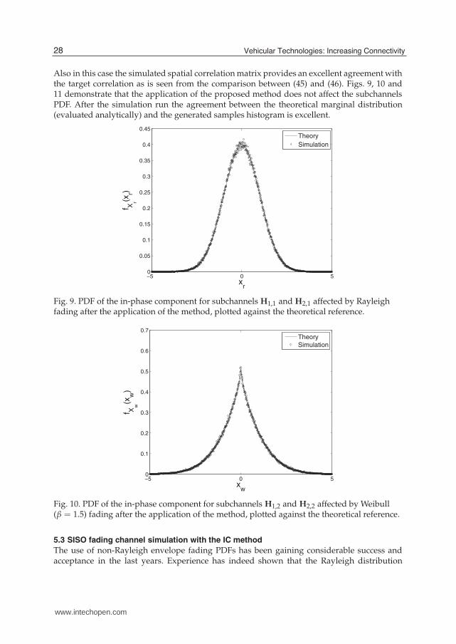
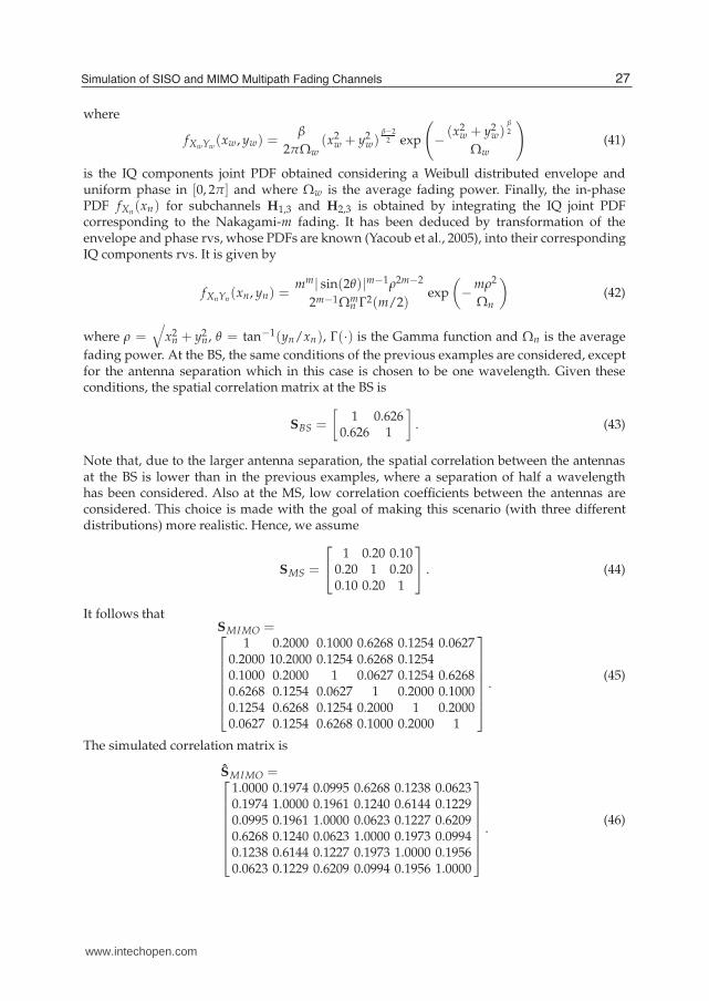
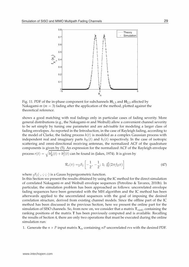
Also in this case the simulated spatial correlation matrix provides an excellent agreement withthe target correlation as is seen from the comparison between (45) and (46). Figs. 9, 10 and11 demonstrate that the application of the proposed method does not affect the subchannelsPDF. After the simulation run the agreement between the theoretical marginal distribution(evaluated analytically) and the generated samples histogram is excellent.

−5 0 50

0.05

0.1

0.15

0.2

0.25

0.3

0.35

0.4

0.45

xr

f Xr(x

r)

Theory

Simulation

Fig. 9. PDF of the in-phase component for subchannels H1,1 and H2,1 affected by Rayleighfading after the application of the method, plotted against the theoretical reference.

−5 0 50

0.1

0.2

0.3

0.4

0.5

0.6

0.7

xw

f Xw

(xw

)

Theory

Simulation

Fig. 10. PDF of the in-phase component for subchannels H1,2 and H2,2 affected by Weibull(β = 1.5) fading after the application of the method, plotted against the theoretical reference.

5.3 SISO fading channel simulation with the IC method

The use of non-Rayleigh envelope fading PDFs has been gaining considerable success andacceptance in the last years. Experience has indeed shown that the Rayleigh distribution


www.intechopen.com

−5 0 50

0.1

0.2

0.3

0.4

0.5

0.6

0.7

0.8

xn

f Xn

(xn)

Theory

Simulation

Fig. 11. PDF of the in-phase component for subchannels H1,3 and H2,3 affected byNakagami-m (m = 3) fading after the application of the method, plotted against thetheoretical reference.

shows a good matching with real fadings only in particular cases of fading severity. Moregeneral distributions (e.g., the Nakagami-m and Weibull) allow a convenient channel severityto be set simply by tuning one parameter and are advisable for modeling a larger class offading envelopes. As reported in the Introduction, in the case of Rayleigh fading, according tothe model of Clarke, the fading process h(t) is modeled as a complex Gaussian process withindependent real and imaginary parts hR(t) and hI(t) respectively. In the case of isotropicscattering and omni-directional receiving antennas, the normalized ACF of the quadraturecomponents is given by (5). An expression for the normalized ACF of the Rayleigh envelope

process r(t) =√

h2R(t) + h2

I (t) can be found in (Jakes, 1974). It is given by

Rr(τ) =2 F1

[

− 1

2, − 1

2; 1; J2

0 (2π fDτ)

]

(47)

where 2F1(·, ·; ·; ·) is a Gauss hypergeometric function.In this Section we present the results obtained by using the IC method for the direct simulationof correlated Nakagami-m and Weibull envelope sequences (Petrolino & Tavares, 2010b). Inparticular, the simulation problem has been approached as follows: uncorrelated envelopefading sequences have been generated with the MH algorithm and the IC method has beenafterwards applied to the uncorrelated sequences with the goal of imposing the desiredcorrelation structure, derived from existing channel models. Since the offline part of the ICmethod has been discussed in the previous Section, here we present the online part for thesimulation of SISO channels. So, from now on, we consider that a matrix Trank, containing theranking positions of the matrix T has been previously computed and is available. Recallingthe results of Section 4, there are only two operations that must be executed during the onlinesimulation run:

1. Generate the n × P input matrix Xin containing nP uncorrelated rvs with the desired PDF.


www.intechopen.com

2. Create matrix X which is a rearranged version of Xin according to the ranks contained inTrank to get the desired ACF.

Each of the n rows of X represents an P-samples fading sequence which can be used forchannel simulation.

5.3.1 Simulation of a SISO channel affected by Nakagami-m fading

In 1960, M. Nakagami proposed a PDF which models well the signal amplitude fading in alarge range of propagation scenarios. A rv RN is Nakagami-m distributed if its PDF followsthe distribution (Nakagami, 1960)

fRN(r) =

2mmr2m−1

Γ(m)Ωm exp

(

−mr2

Ω

)

, r ≥ 0, m >1

2(48)

where Γ(·) is the gamma function, Ω = E[R2N ] is the mean power and

m = Ω2/(R2N − Ω)2 ≥ 1

2 is the Nakagami-m fading parameter which controls the depth ofthe fading amplitude.For m = 1 the Nakagami model coincides with the Rayleigh model, while values of m < 1correspond to more severe fading than Rayleigh and values of m > 1 to less severe fadingthan Rayleigh. The Nakagami-m envelope ACF is found as (Filho et al., 2007)

RRN(τ) =

ΩΓ2(m + 12 )

mΓ2(m)2F1

[

− 1

2, − 1

2; m; ρ(τ)

]

(49)

where ρ(τ) is an autocorrelation coefficient (ACC) which depends on the propagationscenario. In this example and without loss of generality, we consider the isotropic scenariowith uniform distributed waves angles of arrival for which ρ(τ) = J2

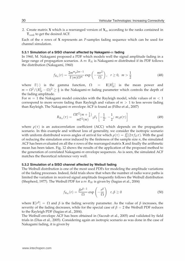
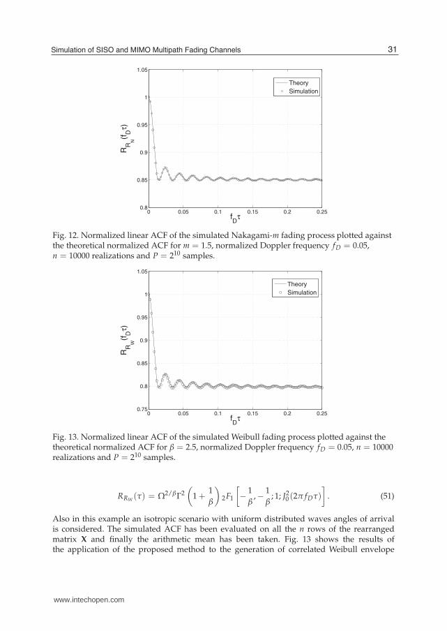
0 (2π fDτ). With the goalof reducing the simulation error induced by the finiteness of the sample size n, the simulatedACF has been evaluated on all the n rows of the rearranged matrix X and finally the arithmeticmean has been taken. Fig. 12 shows the results of the application of the proposed method tothe generation of correlated Nakagami-m envelope sequences. As is seen, the simulated ACFmatches the theoretical reference very well.

5.3.2 Simulation of a SISO channel affected by Weibull fading

The Weibull distribution is one of the most used PDFs for modeling the amplitude variationsof the fading processes. Indeed, field trials show that when the number of radio wave paths islimited the variation in received signal amplitude frequently follows the Weibull distribution(Shepherd, 1977). The Weibull PDF for a rv RW is given by (Sagias et al., 2004)

fRW(r) =

βrβ−1

Ωexp

(

− rβ

Ω

)

r, β ≥ 0 (50)

where E[rβ] = Ω and β is the fading severity parameter. As the value of β increases, theseverity of the fading decreases, while for the special case of β = 2 the Weibull PDF reducesto the Rayleigh PDF (Sagias et al., 2004).The Weibull envelope ACF has been obtained in (Yacoub et al., 2005) and validated by fieldtrials in (Dias et al., 2005). Considering again an isotropic scenario as was done in the case ofNakagami fading, it is given by


www.intechopen.com

0 0.05 0.1 0.15 0.2 0.250.8

0.85

0.9

0.95

1

1.05

fD

τ

RR

N

(fD

τ)

Theory

Simulation

Fig. 12. Normalized linear ACF of the simulated Nakagami-m fading process plotted againstthe theoretical normalized ACF for m = 1.5, normalized Doppler frequency fD = 0.05,n = 10000 realizations and P = 210 samples.

0 0.05 0.1 0.15 0.2 0.250.75

0.8

0.85

0.9

0.95

1

1.05

fD

τ

RR

W

(fD

τ)

Theory

Simulation

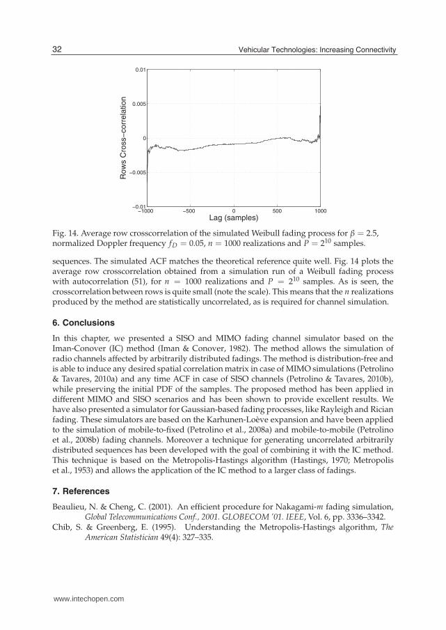
Fig. 13. Normalized linear ACF of the simulated Weibull fading process plotted against thetheoretical normalized ACF for β = 2.5, normalized Doppler frequency fD = 0.05, n = 10000realizations and P = 210 samples.

RRW(τ) = Ω2/βΓ2

(

1 +1

β

)

2F1

[

− 1

β,− 1

β; 1; J2

0 (2π fDτ)

]

. (51)

Also in this example an isotropic scenario with uniform distributed waves angles of arrivalis considered. The simulated ACF has been evaluated on all the n rows of the rearrangedmatrix X and finally the arithmetic mean has been taken. Fig. 13 shows the results ofthe application of the proposed method to the generation of correlated Weibull envelope


www.intechopen.com

−1000 −500 0 500 1000−0.01

−0.005

0

0.005

0.01

Lag (samples)

Ro

ws C

ross−

co

rre

latio

n

Fig. 14. Average row crosscorrelation of the simulated Weibull fading process for β = 2.5,normalized Doppler frequency fD = 0.05, n = 1000 realizations and P = 210 samples.

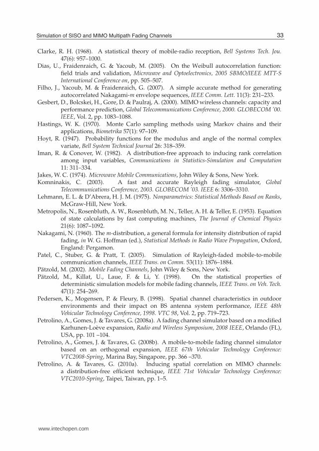
sequences. The simulated ACF matches the theoretical reference quite well. Fig. 14 plots theaverage row crosscorrelation obtained from a simulation run of a Weibull fading processwith autocorrelation (51), for n = 1000 realizations and P = 210 samples. As is seen, thecrosscorrelation between rows is quite small (note the scale). This means that the n realizationsproduced by the method are statistically uncorrelated, as is required for channel simulation.

6. Conclusions

In this chapter, we presented a SISO and MIMO fading channel simulator based on theIman-Conover (IC) method (Iman & Conover, 1982). The method allows the simulation ofradio channels affected by arbitrarily distributed fadings. The method is distribution-free andis able to induce any desired spatial correlation matrix in case of MIMO simulations (Petrolino& Tavares, 2010a) and any time ACF in case of SISO channels (Petrolino & Tavares, 2010b),while preserving the initial PDF of the samples. The proposed method has been applied indifferent MIMO and SISO scenarios and has been shown to provide excellent results. Wehave also presented a simulator for Gaussian-based fading processes, like Rayleigh and Ricianfading. These simulators are based on the Karhunen-Loève expansion and have been appliedto the simulation of mobile-to-fixed (Petrolino et al., 2008a) and mobile-to-mobile (Petrolinoet al., 2008b) fading channels. Moreover a technique for generating uncorrelated arbitrarilydistributed sequences has been developed with the goal of combining it with the IC method.This technique is based on the Metropolis-Hastings algorithm (Hastings, 1970; Metropoliset al., 1953) and allows the application of the IC method to a larger class of fadings.

7. References

Beaulieu, N. & Cheng, C. (2001). An efficient procedure for Nakagami-m fading simulation,Global Telecommunications Conf., 2001. GLOBECOM ’01. IEEE, Vol. 6, pp. 3336–3342.

Chib, S. & Greenberg, E. (1995). Understanding the Metropolis-Hastings algorithm, TheAmerican Statistician 49(4): 327–335.


www.intechopen.com

Clarke, R. H. (1968). A statistical theory of mobile-radio reception, Bell Systems Tech. Jou.47(6): 957–1000.

Dias, U., Fraidenraich, G. & Yacoub, M. (2005). On the Weibull autocorrelation function:field trials and validation, Microwave and Optoelectronics, 2005 SBMO/IEEE MTT-SInternational Conference on, pp. 505–507.

Filho, J., Yacoub, M. & Fraidenraich, G. (2007). A simple accurate method for generatingautocorrelated Nakagami-m envelope sequences, IEEE Comm. Lett. 11(3): 231–233.

Gesbert, D., Bolcskei, H., Gore, D. & Paulraj, A. (2000). MIMO wireless channels: capacity andperformance prediction, Global Telecommunications Conference, 2000. GLOBECOM ’00.IEEE, Vol. 2, pp. 1083–1088.

Hastings, W. K. (1970). Monte Carlo sampling methods using Markov chains and theirapplications, Biometrika 57(1): 97–109.

Hoyt, R. (1947). Probability functions for the modulus and angle of the normal complexvariate, Bell System Technical Journal 26: 318–359.

Iman, R. & Conover, W. (1982). A distribution-free approach to inducing rank correlationamong input variables, Communications in Statistics-Simulation and Computation11: 311–334.

Jakes, W. C. (1974). Microwave Mobile Communications, John Wiley & Sons, New York.Komninakis, C. (2003). A fast and accurate Rayleigh fading simulator, Global

Telecommunications Conference, 2003. GLOBECOM ’03. IEEE 6: 3306–3310.Lehmann, E. L. & D’Abrera, H. J. M. (1975). Nonparametrics: Statistical Methods Based on Ranks,

McGraw-Hill, New York.Metropolis, N., Rosenbluth, A. W., Rosenbluth, M. N., Teller, A. H. & Teller, E. (1953). Equation

of state calculations by fast computing machines, The Journal of Chemical Physics21(6): 1087–1092.

Nakagami, N. (1960). The m-distribution, a general formula for intensity distribution of rapidfading, in W. G. Hoffman (ed.), Statistical Methods in Radio Wave Propagation, Oxford,England: Pergamon.

Patel, C., Stuber, G. & Pratt, T. (2005). Simulation of Rayleigh-faded mobile-to-mobilecommunication channels, IEEE Trans. on Comm. 53(11): 1876–1884.

Pätzold, M. (2002). Mobile Fading Channels, John Wiley & Sons, New York.Pätzold, M., Killat, U., Laue, F. & Li, Y. (1998). On the statistical properties of

deterministic simulation models for mobile fading channels, IEEE Trans. on Veh. Tech.47(1): 254–269.

Pedersen, K., Mogensen, P. & Fleury, B. (1998). Spatial channel characteristics in outdoorenvironments and their impact on BS antenna system performance, IEEE 48thVehicular Technology Conference, 1998. VTC 98, Vol. 2, pp. 719–723.

Petrolino, A., Gomes, J. & Tavares, G. (2008a). A fading channel simulator based on a modifiedKarhunen-Loève expansion, Radio and Wireless Symposium, 2008 IEEE, Orlando (FL),USA, pp. 101 –104.

Petrolino, A., Gomes, J. & Tavares, G. (2008b). A mobile-to-mobile fading channel simulatorbased on an orthogonal expansion, IEEE 67th Vehicular Technology Conference:VTC2008-Spring, Marina Bay, Singapore, pp. 366 –370.

Petrolino, A. & Tavares, G. (2010a). Inducing spatial correlation on MIMO channels:a distribution-free efficient technique, IEEE 71st Vehicular Technology Conference:VTC2010-Spring, Taipei, Taiwan, pp. 1–5.


www.intechopen.com

Petrolino, A. & Tavares, G. (2010b). A simple method for the simulation of autocorrelatedand arbitrarily distributed envelope fading processes, IEEE International Workshop onSignal Processing Advances in Wireless Communications., Marrakech, Morocco.

Pop, M. & Beaulieu, N. (2001). Limitations of sum-of-sinusoids fading channel simulators,IEEE Trans. on Comm. 49(4): 699–708.

Sagias, N., Zogas, D., Karagiannidis, G. & Tombras, G. (2004). Channel capacity andsecond-order statistics in Weibull fading, IEEE Comm. Lett. 8(6): 377–379.

Shepherd, N. (1977). Radio wave loss deviation and shadow loss at 900 MHz, IEEE Trans. onVeh. Tech. 26(4): 309–313.

Smith, J. I. (1975). A computer generated multipath fading simulation for mobile radio, IEEETrans. on Veh. Tech. 24(3): 39–40.

Tierney, L. (1994). Markov chains for exploring posterior distributions, Annals of Statistics22(4): 1701–1728.

Van Trees, H. L. (1968). Detection, Estimation, and Modulation Theory - Part I, Wiley, New York.Vehicular Technology Society Committee on Radio Propagation (1988). Coverage prediction

for mobile radio systems operating in the 800/900 MHz frequency range, IEEE Trans.on Veh. Tech. 37(1): 3–72.

Wang, C. (2006). Modeling MIMO fading channels: Background, comparison andsome progress, Communications, Circuits and Systems Proceedings, 2006 InternationalConference on, Vol. 2, pp. 664–669.

Weibull, W. (1951). A statistical distribution function of wide applicability, ASME Jou. ofApplied Mechanics, Trans. of the American Society of Mechanical Engineers 18(3): 293–297.

Yacoub, M., Fraidenraich, G. & Santos Filho, J. (2005). Nakagami-m phase-envelope jointdistribution, Electr. Lett. 41(5): 259–261.

Young, D. & Beaulieu, N. (2000). The generation of correlated Rayleigh random variates byinverse discrete Fourier transform, IEEE Trans. on Comm. 48(7): 1114–1127.


www.intechopen.com

Vehicular Technologies: Increasing ConnectivityEdited by Dr Miguel Almeida

ISBN 978-953-307-223-4Hard cover, 448 pagesPublisher InTechPublished online 11, April, 2011Published in print edition April, 2011

InTech EuropeUniversity Campus STeP Ri Slavka Krautzeka 83/A 51000 Rijeka, Croatia Phone: +385 (51) 770 447 Fax: +385 (51) 686 166www.intechopen.com

InTech ChinaUnit 405, Office Block, Hotel Equatorial Shanghai No.65, Yan An Road (West), Shanghai, 200040, China

Phone: +86-21-62489820 Fax: +86-21-62489821

This book provides an insight on both the challenges and the technological solutions of several approaches,which allow connecting vehicles between each other and with the network. It underlines the trends onnetworking capabilities and their issues, further focusing on the MAC and Physical layer challenges. Rangingfrom the advances on radio access technologies to intelligent mechanisms deployed to enhance cooperativecommunications, cognitive radio and multiple antenna systems have been given particular highlight.

How to referenceIn order to correctly reference this scholarly work, feel free to copy and paste the following:

Antonio Petrolino and Gonc alo Tavares (2011). Simulation of SISO and MIMO Multipath Fading Channels,Vehicular Technologies: Increasing Connectivity, Dr Miguel Almeida (Ed.), ISBN: 978-953-307-223-4, InTech,Available from: http://www.intechopen.com/books/vehicular-technologies-increasing-connectivity/simulation-of-siso-and-mimo-multipath-fading-channels

Simulation of SISO and MIMO Multipath Fading...

Documents

Transcript of Simulation of SISO and MIMO Multipath Fading...