Link Budget 4G · Average attenuation in -10αlog(d) Shadowing Fast fading Received signal ......
16
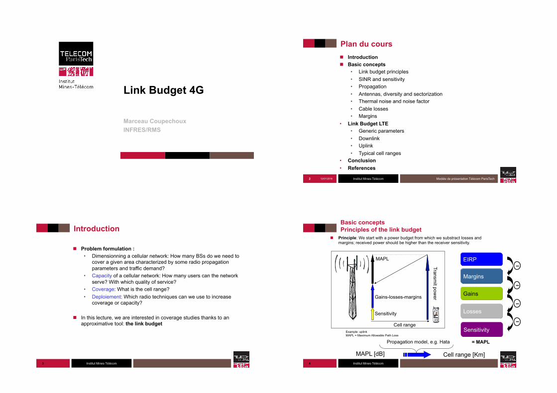
Institut Mines-Télécom Link Budget 4G Marceau Coupechoux INFRES/RMS Institut Mines-Télécom Plan du cours ! Introduction ! Basic concepts • Link budget principles • SINR and sensitivity • Propagation • Antennas, diversity and sectorization • Thermal noise and noise factor • Cable losses • Margins • Link Budget LTE • Generic parameters • Downlink • Uplink • Typical cell ranges • Conclusion • References 12/01/2016 Modèle de présentation Télécom ParisTech 2 Institut Mines-Télécom 3 Introduction ! Problem formulation : • Dimensionning a cellular network: How many BSs do we need to cover a given area characterized by some radio propagation parameters and traffic demand? • Capacity of a cellular network: How many users can the network serve? With which quality of service? • Coverage: What is the cell range? • Deploiement: Which radio techniques can we use to increase coverage or capacity? ! In this lecture, we are interested in coverage studies thanks to an approximative tool: the link budget Institut Mines-Télécom 4 Basic concepts Principles of the link budget ! Principle: We start with a power budget from which we substract losses and margins; received power should be higher than the receiver sensitivity. Cell range Sensitivity Gains-losses-margins Transmit power MAPL Example: uplink MAPL = Maximum Allowable Path Loss MAPL [dB] Cell range [Km] Propagation model, e.g. Hata Sensitivity EIRP Losses Gains = MAPL Margins
Transcript of Link Budget 4G · Average attenuation in -10αlog(d) Shadowing Fast fading Received signal ......
Institut Mines-Télécom
Link Budget 4G
Marceau Coupechoux INFRES/RMS
Institut Mines-Télécom
Plan du cours ! Introduction ! Basic concepts
• Link budget principles • SINR and sensitivity • Propagation • Antennas, diversity and sectorization • Thermal noise and noise factor • Cable losses • Margins
• Link Budget LTE • Generic parameters • Downlink • Uplink • Typical cell ranges
• Conclusion • References
12/01/2016 Modèle de présentation Télécom ParisTech 2
Institut Mines-Télécom 3
Introduction
! Problem formulation : • Dimensionning a cellular network: How many BSs do we need to
cover a given area characterized by some radio propagation parameters and traffic demand?
• Capacity of a cellular network: How many users can the network serve? With which quality of service?
• Coverage: What is the cell range? • Deploiement: Which radio techniques can we use to increase
coverage or capacity?
! In this lecture, we are interested in coverage studies thanks to an approximative tool: the link budget
Institut Mines-Télécom 4
Basic concepts Principles of the link budget
! Principle: We start with a power budget from which we substract losses and margins; received power should be higher than the receiver sensitivity.
Cell range
Sensitivity
Gains-losses-margins
Transmit pow
er
MAPL
Example: uplink MAPL = Maximum Allowable Path Loss
MAPL [dB] Cell range [Km]
Propagation model, e.g. Hata
Sensitivity
EIRP
Losses
Gains
= MAPL
Margins
Institut Mines-Télécom 5
Basic concepts Principles of the link budget
Uplink Link Budget
Downlink Link Budget
MAPLUL = Uplink maximum allowable path-loss
MAPLDL = Downlink maximum allowable path-loss
MAPL = MIN(MAPLUL,MAPLDL)
Cell range
A MS at cell edge transmits at maximum power
BS transmits ar maximum power
NB: Uplink and Downlink budgets are independent
Institut Mines-Télécom 6
Basic concepts Principles of the link budget
! The MAPL is the minimum of the uplink and downlink MAPLs.
! To increase coverage, it is needed to identify the limiting link: • Uplink limited: MAPLul < MAPLdl • Downlink limited: MAPLdl < MAPLul
! Coverage extension is done by using appropriate radio techniques: • Uplink limited network:
─ Receive diversity (2 or 4 antennas), ─ Tower Mounted Amplifier (TMA).
• Downlink limited network: ─ High power amplifier, ─ Transmit diversity, ─ Low loss BS configuration.
Institut Mines-Télécom
Basic concepts SINR and sensitivity
! Sensitivity = minimum power needed to guarantee a certain quality of service or a certain throughput in presence of noise only
! Dedicated channel technologies (UMTS R99, GSM): There is a target SNR or SINR γ*. Below this threshold, quality of service is not sufficient.
! Shared channel technologies (HSDPA, LTE): Throughput is an
increasing function of the SNR/SINR. We deduce from the target throughput at cell edge, the SNR or SINR threshold γ* to be reached.
! From noise power and SNR threshold, we deduce the sensitivity:
! In a link budget, co-channel interferences are taken into account in an interference margin.
7 Institut Mines-Télécom
Basic concepts SINR and sensitivity
! Reminder on logarithmique scale, dB and dBm
! We use the logarithmic scale to represent signal to (interference plus) noise ratios
X_dB = 10 log10(X_linear) => X_linear = 10(X_dB/10)
! SNRdB = 10 log10(SNRlinear)
! The dB milliwatt or dBm:
P_dBm = 10 log10(P_mW).
! Ex: SNRlinear= 2 <=> SNRdB = 3 dB
! Be careful: subscripts are rarely used (but it does not mean that 2 = 3 (!))
8
10 dB = 10 times 7 dB = 5 times
3 dB = 2 times 0 dB = 1 times
-3 dB = ½ times -10 dB = 1/10 times
-13 dB = 1/20 times -17 dB = 1/50 times
Institut Mines-Télécom
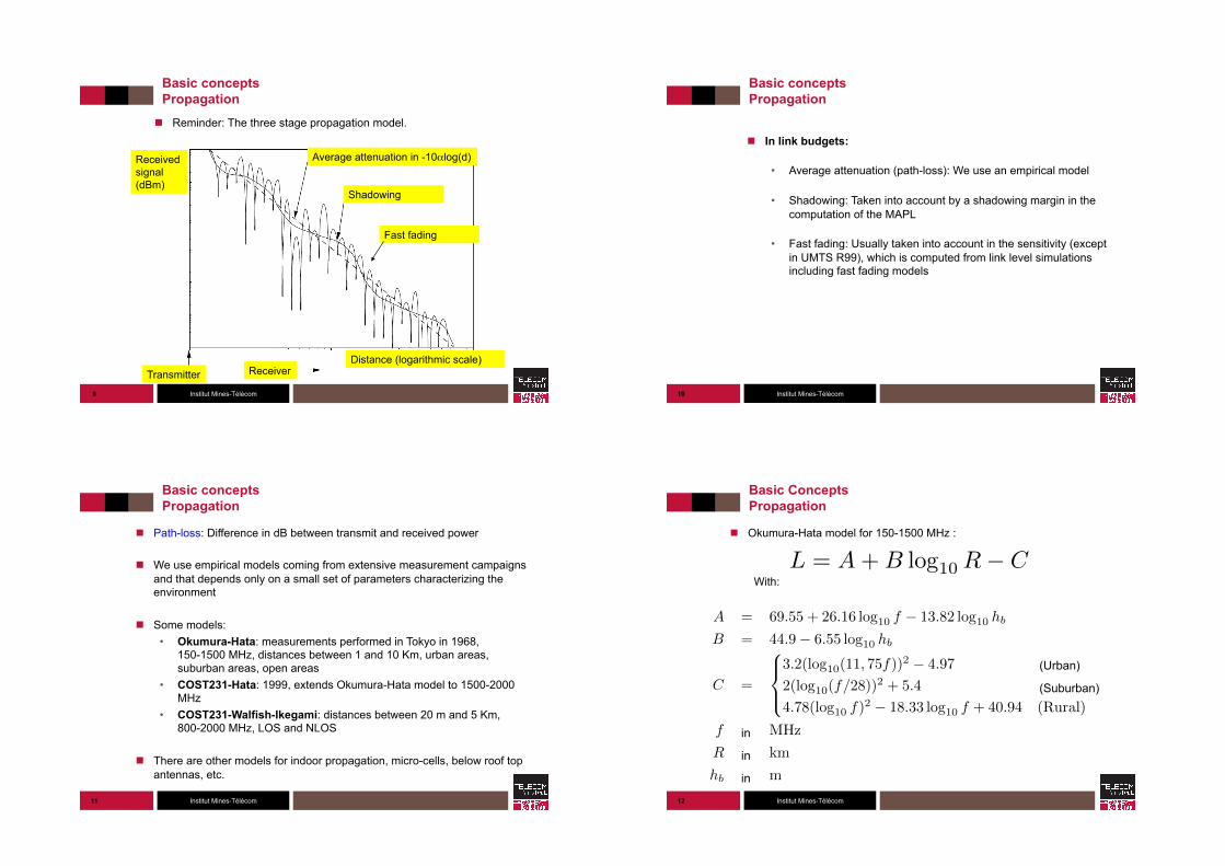
Basic concepts Propagation
! Reminder: The three stage propagation model.
9
Average attenuation in -10αlog(d)
Shadowing
Fast fading
Received signal (dBm)
Transmitter Receiver Distance (logarithmic scale)
Institut Mines-Télécom
Basic concepts Propagation
! In link budgets: • Average attenuation (path-loss): We use an empirical model
• Shadowing: Taken into account by a shadowing margin in the
computation of the MAPL
• Fast fading: Usually taken into account in the sensitivity (except in UMTS R99), which is computed from link level simulations including fast fading models
10
Institut Mines-Télécom
Basic concepts Propagation
! Path-loss: Difference in dB between transmit and received power
! We use empirical models coming from extensive measurement campaigns and that depends only on a small set of parameters characterizing the environment
! Some models: • Okumura-Hata: measurements performed in Tokyo in 1968,
150-1500 MHz, distances between 1 and 10 Km, urban areas, suburban areas, open areas
• COST231-Hata: 1999, extends Okumura-Hata model to 1500-2000 MHz
• COST231-Walfish-Ikegami: distances between 20 m and 5 Km, 800-2000 MHz, LOS and NLOS
! There are other models for indoor propagation, micro-cells, below roof top antennas, etc.
11 Institut Mines-Télécom
Basic Concepts Propagation
! Okumura-Hata model for 150-1500 MHz :
With:
12
L = A+B log10 R� C
A = 69.55 + 26.16 log10 f � 13.82 log10 hb
B = 44.9� 6.55 log10 hb
C =
8><
>:
3.2(log10(11, 75f))2 � 4.97 (Urbain)
2(log10(f/28))2 + 5.4 (Suburbain)
4.78(log10 f)2 � 18.33 log10 f + 40.94 (Rural)
f en MHz
R en km
hb en m
(Urban)
(Suburban)
in
in
in
Institut Mines-Télécom
Basic concepts Propagation
! COST231-Hata model for 1500-2000 MHz (urban environment) :
With:
13
L = A+B log10 R� C
A = 46.3 + 33.9 log10 f � 13.82 log10 hb
B = 44.9� 6.55 log10 hb
C = (1.1 log10 f � 0.7)hm � (1.56 log10 f � 0.8)� 3
f en MHz
R en km
hb en m
hm en m
in
in
in
in
Institut Mines-Télécom
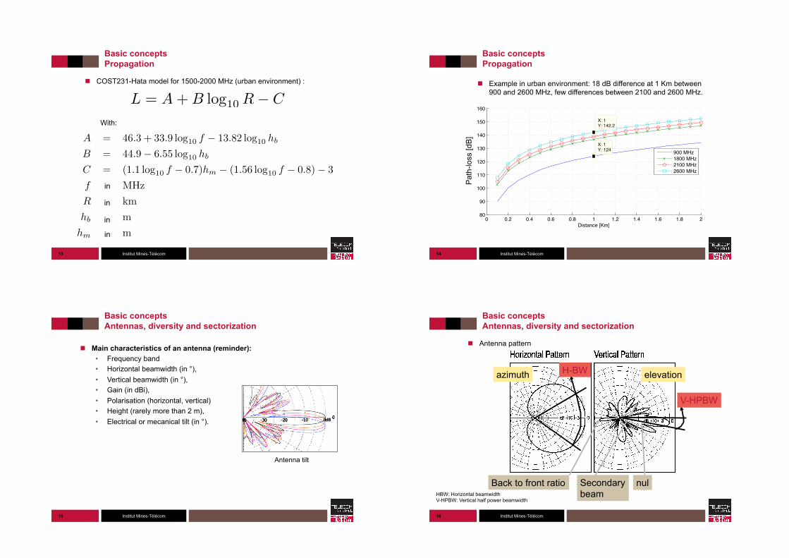
Basic concepts Propagation
! Example in urban environment: 18 dB difference at 1 Km between 900 and 2600 MHz, few differences between 2100 and 2600 MHz.
14
0 0.2 0.4 0.6 0.8 1 1.2 1.4 1.6 1.8 280
90
100
110
120
130
140
150
160
X: 1Y: 142.2
X: 1Y: 124
Distance [Km]
Atte
nuat
ion
[dB]
900 MHz1800 MHz2100 MHz2600 MHz
Pat
h-lo
ss [d
B]
Institut Mines-Télécom 15
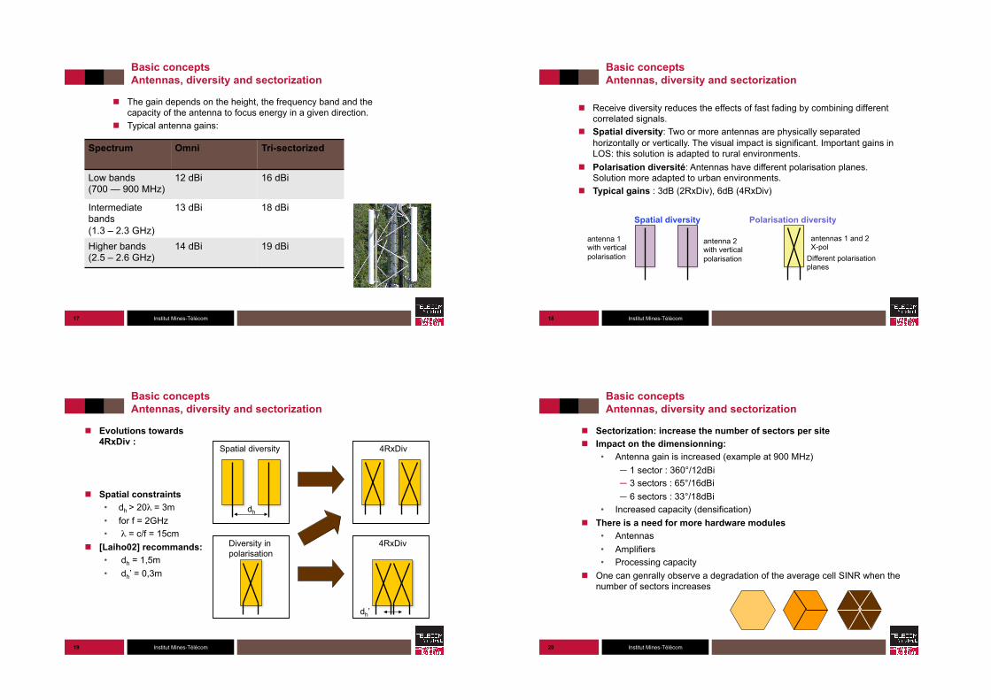
Basic concepts Antennas, diversity and sectorization
! Main characteristics of an antenna (reminder): • Frequency band • Horizontal beamwidth (in °), • Vertical beamwidth (in °), • Gain (in dBi), • Polarisation (horizontal, vertical) • Height (rarely more than 2 m), • Electrical or mecanical tilt (in °).
Antenna tilt
Institut Mines-Télécom 16
Basic concepts Antennas, diversity and sectorization
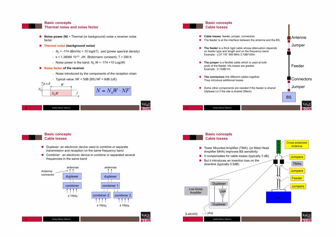
! Antenna pattern
azimuth elevation
Secondary beam
Back to front ratio nul
H-BW
V-HPBW
HBW: Horizontal beamwidth V-HPBW: Vertical half power beamwidth
Institut Mines-Télécom
Basic concepts Antennas, diversity and sectorization
! The gain depends on the height, the frequency band and the capacity of the antenna to focus energy in a given direction.
! Typical antenna gains:
17
Spectrum Omni Tri-sectorized
Low bands (700 — 900 MHz)
12 dBi 16 dBi
Intermediate bands (1.3 – 2.3 GHz)
13 dBi 18 dBi
Higher bands (2.5 – 2.6 GHz)
14 dBi 19 dBi
Institut Mines-Télécom 18
Basic concepts Antennas, diversity and sectorization
! Receive diversity reduces the effects of fast fading by combining different correlated signals.
! Spatial diversity: Two or more antennas are physically separated horizontally or vertically. The visual impact is significant. Important gains in LOS: this solution is adapted to rural environments.
! Polarisation diversité: Antennas have different polarisation planes. Solution more adapted to urban environments.
! Typical gains : 3dB (2RxDiv), 6dB (4RxDiv)
Spatial diversity
antenna 1 with vertical polarisation
Polarisation diversity
antennas 1 and 2 X-pol
Different polarisation planes
antenna 2 with vertical polarisation
Institut Mines-Télécom 19
Basic concepts Antennas, diversity and sectorization
! Evolutions towards 4RxDiv :
! Spatial constraints • dh > 20λ = 3m • for f = 2GHz $• λ = c/f = 15cm
! [Laiho02] recommands: • dh = 1,5m • dh’ = 0,3m
Spatial diversity 4RxDiv
Diversity in polarisation
4RxDiv
dh
dh’
Institut Mines-Télécom 20
Basic concepts Antennas, diversity and sectorization
! Sectorization: increase the number of sectors per site ! Impact on the dimensionning:
• Antenna gain is increased (example at 900 MHz) ─ 1 sector : 360°/12dBi ─ 3 sectors : 65°/16dBi ─ 6 sectors : 33°/18dBi
• Increased capacity (densification) ! There is a need for more hardware modules
• Antennas • Amplifiers • Processing capacity
! One can genrally observe a degradation of the average cell SINR when the number of sectors increases
Institut Mines-Télécom 21
Basic concepts Thermal noise and noise factor
! Noise power (N) = Thermal (or background) noise x receiver noise factor
! Thermal noise (background noise)
- N0 = -174 dBm/Hz = 10 log(kT), psd (power spectral density)
- k = 1.38066 10-23 J/K (Boltzmann constant), T = 290 K
- Noise power in the band: N0 W = -174 +10 Log(W)
! Noise factor of the receiver
- Noise introduced by the components of the reception chain
- Typical value: NF = 5dB (BS) NF = 8dB (UE)
N0W
p.s.d
f N0
W
NFWNN ⋅= 0
Institut Mines-Télécom 22
Basic concepts Cable losses
! Cable losses: feeder, jumper, connectors ! The feeder is at the interface between the antenna and the BS.
! The feeder is a thick rigid cable whose attenuation depends on feeder type and length and on the frequency band. Example : LCF 7/8’’ 900 MHz 3.7dB/100m
! The jumper is a flexible cable which is used at both ends of the feeder. His losses are greater. Example : 0.15dB/1m
! The connectors link different cables together. They introduce additional losses.
! Some other components are needed if the feeder is shared (diplexer) or if the site is shared (filters).
BS
Antenne
Jumper
Jumper
Feeder
Connectors
Institut Mines-Télécom 23
Basic concepts Cable losses
! Duplexer: an electronic device used to combine or separate transmission and reception on the same frequency band
! Combiner : an electronic device to combine or separated several frequencies in the same band
duplexer
combiner
antennas
4 TRXs
duplexer
combiner 1
antennas
combiner 2 combiner 2
4 TRXs 4 TRXs
Antenna connector
Institut Mines-Télécom 24
Basic concepts Cable losses
! Tower Mounted Amplifier (TMA): (or Mast Head Amplifier MHA) improves BS sensitivity
! It compensates for cable losses (typically 3 dB). ! But it introduces an insertion loss on the
downlink (typically 0.5dB)
BS
Duplexer
Duplexer
LNA
Cross-polarized Antenna
Low Noise Amplifier
TMAs
Jumpers
Feeder
Jumpers
Jumpers
[Laiho02] plug
Institut Mines-Télécom 25
Basic concepts Cable losses
! Noise factor reduction: the global noise factor of a cascade of active and passive components is given by the Friis formula:
! The number of stages depends on the site architecture ! Typically: TMA – Feeder – Connectors – BS (if jumpers are neglected) ! TMA impact is often modeled by the suppression of cable and connectors losses
on the uplink: interesting for high antennas
...111
321
4
21
3
1
21 +
−+
−+
−+=
GGGNF
GGNF
GNFNFNF
Noise factors:
Gains :
F1 F2 F3 F4
G1 G2 G3 G4
[Laiho02]
Institut Mines-Télécom 26
Basic concepts Cable losses
! Example of computation of the noise factor: • NB: passive components have a noise factor equal to their loss • Typical gain of a TMA: 12dB • Typical noise factor of a TMA : 2dB
! Without TMA: NF = 5.3dB ! With TMA: NF = 2.4dB ! Gain brought by the TMA: 2.9dB
Component Gain Noise factor TMA 12dB 2dB Feeder -2dB 2dB Connectors -0.3dB 0.3dB BS - 3dB
Institut Mines-Télécom
Basic concepts Cable losses ! RRU (Remote Radio Unit) or RRH (Remote Radio Head): allows to
move certain functions of the BS in a module close to the antenna
27
BS
Antenna
Jumper
Jumper
Feeder
Transmitters/Receivers (TxRx) Power amplifiers Duplexers Controlers (antennas, O&M) Base Band Boards (BBU)
BS
RRU Transmitters/Receivers (TxRx) Power amplifiers Duplexers Controlers (antennas, O&M)
Base Band Boards (BBU)
Opt
ical
fibe
r (C
PR
I/OB
SA
I)
Institut Mines-Télécom
Basic concepts Margins
! Main margins: • Shadowing margin • Fast fading margin (for UMTS) • Indoor penetration margin (loss) • Interference margin • Body losses
! Body losses: losses introduced by the head of the user when he is in a phone call. Recommanded figure is 3 dB [GSM03.30]. 0dB for visiophonie or data services.
28
Institut Mines-Télécom 29
Basic concepts Margins
! Shadowing margin: shadowing is modeled by a log-normal distribution; the shadowing margin ensures that the signal level is above the sensitivity in the whole cell with a probability of 90% - 95%.
! Shadowing margin depends on the standard deviation of the log-normal
! Standard deviation depends on the environment:
• Close to 8 dB in dense urban, • Close to 6 dB in rural.
! Two approaches: • On the whole cell area, • On the cell border.
Smoy Sseuil
Shadowing margin
Institut Mines-Télécom 30
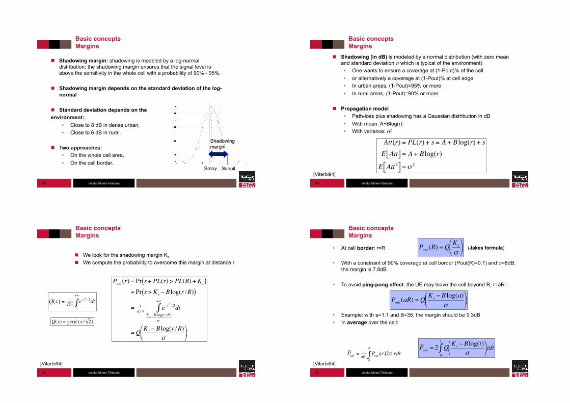
Basic concepts Margins
! Shadowing (in dB) is modeled by a normal distribution (with zero mean and standard deviation σ which is typical of the environment) • One wants to ensure a coverage at (1-Pout)% of the cell • or alternatively a coverage at (1-Pout)% at cell edge • In urban areas, (1-Pout)=95% or more • In rural areas, (1-Pout)=90% or more
! Propagation model • Path-loss plus shadowing has a Gaussian distribution in dB • With mean: A+Blog(r) • With variance: σ2
€
Att(r) = PL(r) + s = A + B log(r) + sE Att[ ] = A + B log(r)
E Att 2[ ] =σ 2
[Viterbi94]
Institut Mines-Télécom 31
Basic concepts Margins
! We look for the shadowing margin Ks ! We compute the probability to overcome this margin at distance r
€
Pout (r) = Pr s+ PL(r) > PL(R) + Ks( )= Pr s > Ks − B log(r /R)( )
= 12π
e−t2 / 2dt
Ks −B log(r /R )σ
+∞
∫
=Q Ks − B log(r /R)σ
'
( )
*
+ ,
∫+∞
−=x
t dtexQ 2/21 2
)(π
€
Q(x) = 12 erfc(x / 2)
[Viterbi94]
Institut Mines-Télécom 32
Basic concepts Margins
• At cell border: r=R
• With a constraint of 90% coverage at cell border (Pout(R)=0.1) and σ=8dB, the margin is 7.8dB
• To avoid ping-pong effect, the UE may leave the cell beyond R, r=aR :
• Example: with a=1.1 and B=35, the margin should be 9.3dB • In average over the cell:
€
Pout (R) =Q Ks
σ
#
$ %
&
' (
€
Pout (aR) =Q Ks − B log(a)σ
$
% &
'
( )
∫=R
outRout rdrrPP0
1 2)(2 ππ
€
P out = 2 Q Ks − B log(t)σ
$
% &
'
( ) tdt
0
1
∫
[Viterbi94]
(Jakes formula)
Institut Mines-Télécom
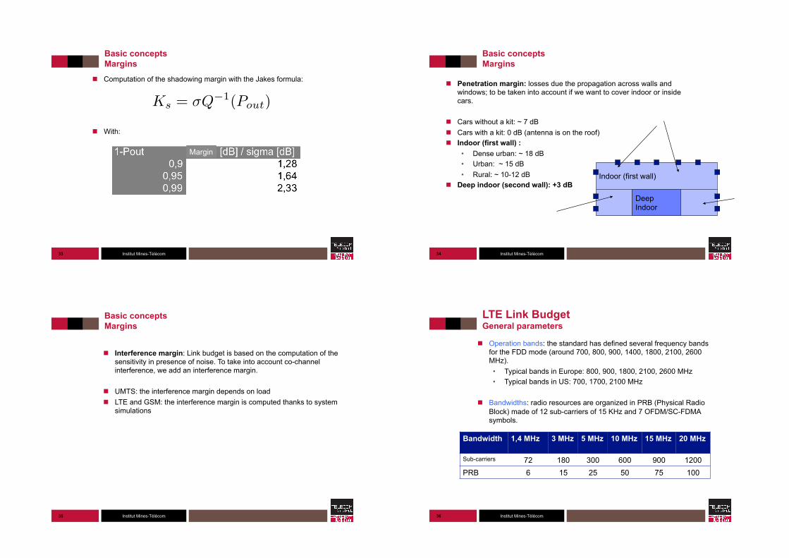
Basic concepts Margins
! Computation of the shadowing margin with the Jakes formula:
! With:
33
Ks
= �Q�1(Pout
)
Margin
Institut Mines-Télécom 34
Basic concepts Margins
! Penetration margin: losses due the propagation across walls and windows; to be taken into account if we want to cover indoor or inside cars.
! Cars without a kit: ~ 7 dB ! Cars with a kit: 0 dB (antenna is on the roof) ! Indoor (first wall) :
• Dense urban: ~ 18 dB • Urban: ~ 15 dB • Rural: ~ 10-12 dB
! Deep indoor (second wall): +3 dB
Indoor (first wall)
Deep Indoor
Institut Mines-Télécom 35
Basic concepts Margins
! Interference margin: Link budget is based on the computation of the sensitivity in presence of noise. To take into account co-channel interference, we add an interference margin.
! UMTS: the interference margin depends on load ! LTE and GSM: the interference margin is computed thanks to system
simulations
Institut Mines-Télécom
LTE Link Budget General parameters
! Operation bands: the standard has defined several frequency bands for the FDD mode (around 700, 800, 900, 1400, 1800, 2100, 2600 MHz). • Typical bands in Europe: 800, 900, 1800, 2100, 2600 MHz • Typical bands in US: 700, 1700, 2100 MHz
! Bandwidths: radio resources are organized in PRB (Physical Radio Block) made of 12 sub-carriers of 15 KHz and 7 OFDM/SC-FDMA symbols.
36
Bandwidth 1,4 MHz 3 MHz 5 MHz 10 MHz 15 MHz 20 MHz
Sub-carriers 72 180 300 600 900 1200 PRB 6 15 25 50 75 100
Institut Mines-Télécom
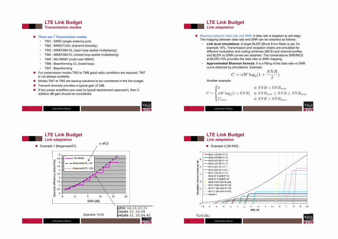
LTE Link Budget Transmission modes
! There are 7 Transmission modes • TM1 : SIMO (single antenna port) • TM2 : MIMO/TxDiv (transmit diversity) • TM3 : MIMO/SM-OL (open loop spatial multiplexing) • TM4 : MIMO/SM-CL (closed loop spatial multiplexing) • TM5 : MU-MIMO (multi-user MIMO) • TM6 : Beamforming CL (losed-loop) • TM7 : Beamforming
! For transmission modes TM3 to TM6 good radio conditions are required. TM7 is not always available.
! Modes TM1 et TM2 are backup solutions to be considered in the link budget. ! Transmit diversity provides a typical gain of 3dB. ! If two power amplifiers are used (a typical deploiement approach), then 3
addition dB gain should be considered.
37 Institut Mines-Télécom
LTE Link Budget Link adaptation
! Mapping between data rate and SNR: A data rate is targeted at cell edge. The mapping between data rate and SNR can be obtained as follows: • Link level simulations: A target BLER (Block Error Rate) is set, for
example 10%. Transmission and reception chains are simulated for different modulation and coding schemes (MCS) and channel profiles and BLER vs SINR curves are obtained. The combinations SNR/MCS at BLER=10% provides the data rate vs SNR mapping.
• Approximated Shannon formula: It is a fitting of the data rate vs SNR curve obtained by simulations. Example:
Another example:
38
C = ↵W log2(1 +SNR
�)
C =
8><
>:
0 si SNR < SNRmin
↵W log2(1 + SNR) si SNRmin
SNR SNRmax
Cmax
si SNR > SNRmax
Institut Mines-Télécom
LTE Link Budget Link adaptation
! Example 1 [Mogensen07] :
39
SNR [dB]
α et β$
Spe
ctra
l effi
cien
cy [b
its/s
/Hz]
Downlink, TU10
Institut Mines-Télécom
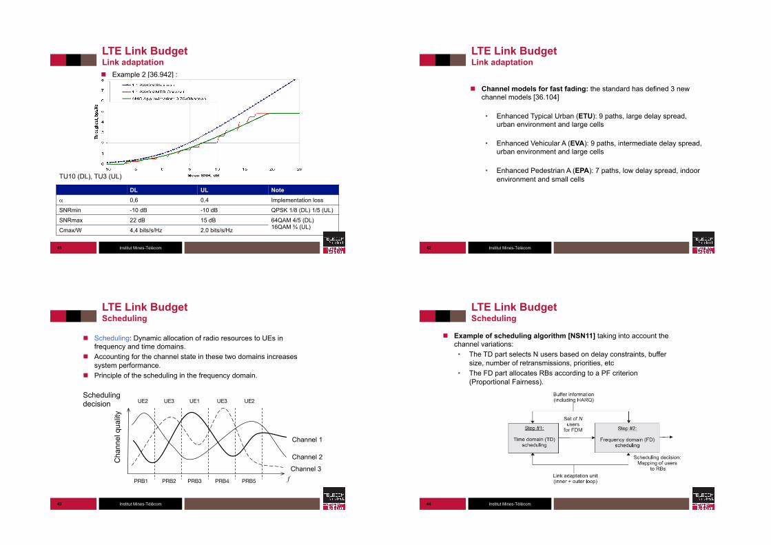
LTE Link Budget Link adaptation ! Example 2 [36.942] :
40
TU10 (DL)
Institut Mines-Télécom
LTE Link Budget Link adaptation ! Example 2 [36.942] :
41
DL UL Note α$ 0,6 0,4 Implementation loss
SNRmin -10 dB -10 dB QPSK 1/8 (DL) 1/5 (UL)
SNRmax 22 dB 15 dB 64QAM 4/5 (DL) 16QAM ¾ (UL) Cmax/W 4,4 bits/s/Hz 2,0 bits/s/Hz
TU10 (DL), TU3 (UL)
Institut Mines-Télécom
LTE Link Budget Link adaptation
! Channel models for fast fading: the standard has defined 3 new channel models [36.104] • Enhanced Typical Urban (ETU): 9 paths, large delay spread,
urban environment and large cells
• Enhanced Vehicular A (EVA): 9 paths, intermediate delay spread, urban environment and large cells
• Enhanced Pedestrian A (EPA): 7 paths, low delay spread, indoor environment and small cells
42
Institut Mines-Télécom
LTE Link Budget Scheduling
! Scheduling: Dynamic allocation of radio resources to UEs in frequency and time domains.
! Accounting for the channel state in these two domains increases system performance.
! Principle of the scheduling in the frequency domain.
43
Qua
lité
du
cana
l
fPRB1 PRB2 PRB3 PRB4 PRB5
Canal UE1
Canal UE2
Canal UE3
Décisions de l'ordonnanceur : UE2 UE3 UE1 UE3 UE2
Scheduling decision
Cha
nnel
qua
lity
Channel 1
Channel 2
Channel 3
Institut Mines-Télécom
LTE Link Budget Scheduling
! Example of scheduling algorithm [NSN11] taking into account the channel variations: • The TD part selects N users based on delay constraints, buffer
size, number of retransmissions, priorities, etc • The FD part allocates RBs according to a PF criterion
(Proportional Fairness).
44
Institut Mines-Télécom
LTE Link Budget Scheduling
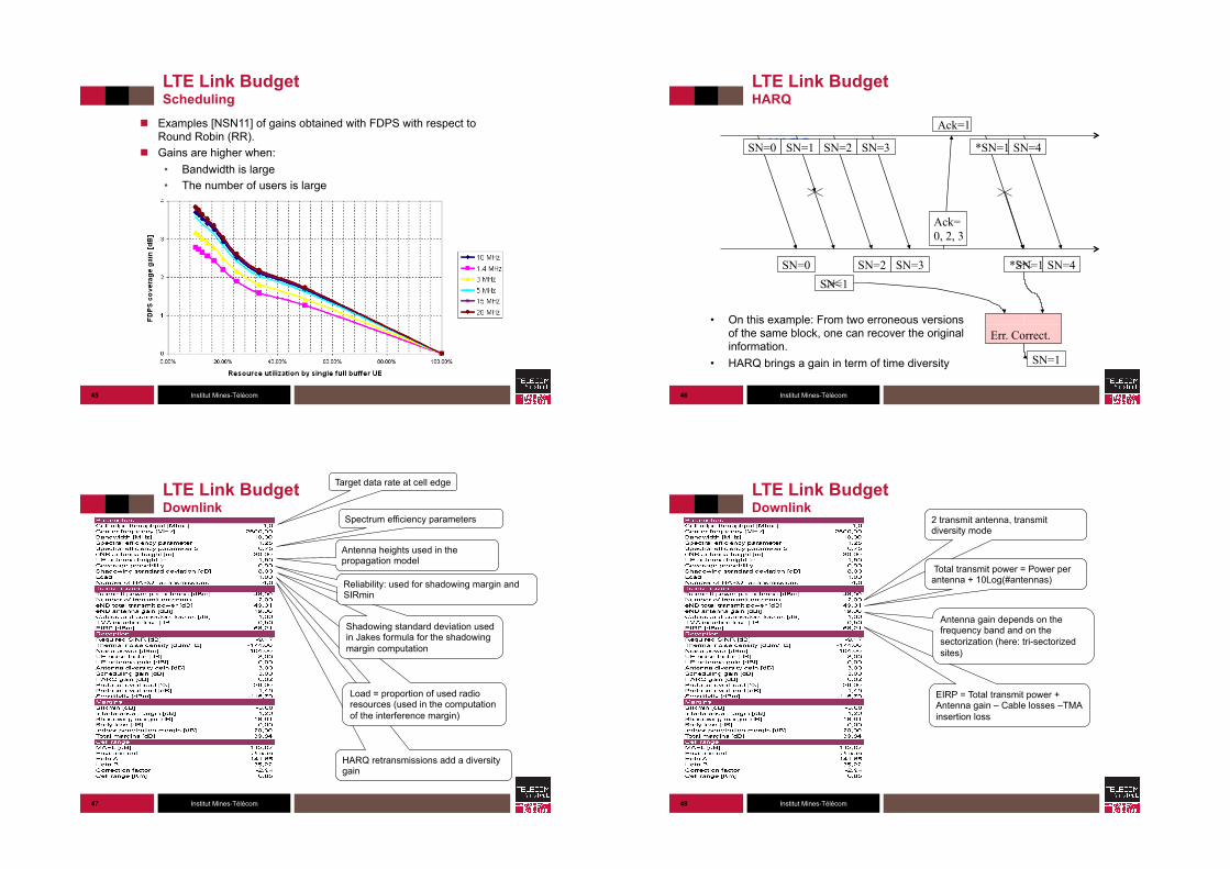
! Examples [NSN11] of gains obtained with FDPS with respect to Round Robin (RR).
! Gains are higher when: • Bandwidth is large • The number of users is large
45 Institut Mines-Télécom
LTE Link Budget HARQ
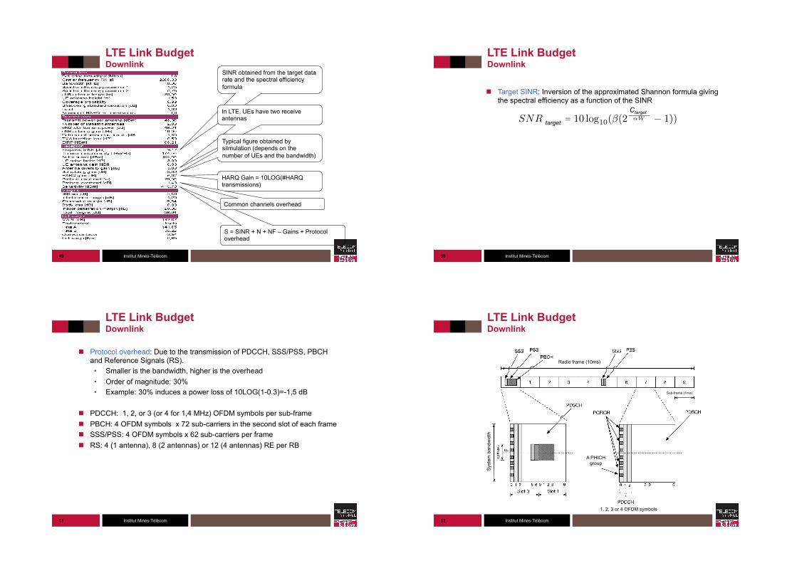
! HARQ :
46
• On this example: From two erroneous versions of the same block, one can recover the original information.
• HARQ brings a gain in term of time diversity
SN=0
SN=0
Ack= 0, 2, 3
Ack=1
SN=1 SN=2
SN=2
SN=3
SN=3
*SN=1
*SN=1
SN=4
SN=4
SN=1
Err. Correct.
SN=1
Institut Mines-Télécom
LTE Link Budget Downlink
47
Target data rate at cell edge
Spectrum efficiency parameters
Antenna heights used in the propagation model
HARQ retransmissions add a diversity gain
Load = proportion of used radio resources (used in the computation of the interference margin)
Shadowing standard deviation used in Jakes formula for the shadowing margin computation
Reliability: used for shadowing margin and SIRmin
Institut Mines-Télécom
LTE Link Budget Downlink
48
2 transmit antenna, transmit diversity mode
Total transmit power = Power per antenna + 10Log(#antennas)
EIRP = Total transmit power + Antenna gain – Cable losses –TMA insertion loss
Antenna gain depends on the frequency band and on the sectorization (here: tri-sectorized sites)
Institut Mines-Télécom
LTE Link Budget Downlink
49
SINR obtained from the target data rate and the spectral efficiency formula
In LTE, UEs have two receive antennas
Typical figure obtained by silmulation (depends on the number of UEs and the bandwidth)
HARQ Gain = 10LOG(#HARQ transmissions)
S = SINR + N + NF – Gains + Protocol overhead
Common channels overhead
Institut Mines-Télécom
LTE Link Budget Downlink
! Target SINR: Inversion of the approximated Shannon formula giving the spectral efficiency as a function of the SINR
50
SNRcible = 10 log10(�(2Ccible↵W � 1))target
Ctarget
Institut Mines-Télécom
LTE Link Budget Downlink
! Protocol overhead: Due to the transmission of PDCCH, SSS/PSS, PBCH and Reference Signals (RS). • Smaller is the bandwidth, higher is the overhead • Order of magnitude: 30% • Example: 30% induces a power loss of 10LOG(1-0.3)=-1,5 dB
! PDCCH: 1, 2, or 3 (or 4 for 1,4 MHz) OFDM symbols per sub-frame ! PBCH: 4 OFDM symbols x 72 sub-carriers in the second slot of each frame ! SSS/PSS: 4 OFDM symbols x 62 sub-carriers per frame ! RS: 4 (1 antenna), 8 (2 antennas) or 12 (4 antennas) RE per RB
51 Institut Mines-Télécom
LTE Link Budget Downlink
! Canaux de contrôle :
52
Radio frame (10ms)
Sub-frame (1ms)
A PHICH group
1, 2, 3 or 4 OFDM symbols
Sys
tem
ban
dwid
th
Institut Mines-Télécom
LTE Link Budget Downlink
! Orders of magnitude:
53
DL Overhead (%)
Institut Mines-Télécom
LTE Link Budget Downlink
54
MI = -10LOG(1-load*SINR/SIRmin)
Jakes Formula
Margins = MI + Shadowing + Body loss + Penetration
Institut Mines-Télécom
LTE Link Budget Downlink
! Interference margin: One obtains by simulation the SIRmin as a function of the coverage required reliability. One then deduces the interference margin from SIRmin and from the target SINRas follows:
55
MI =SNR
SINR
SINR =S
⌘I +N=
1⌘
SIRmin+ 1
SNR
MI =1
1� ⌘ SINRSIRmin
Note 1 : SIRmin depends only on the propagation model and on the required reliability Note 2 : withCOST231-Hata, SIRmin depends only on B (i.e., on hb) and on the reliability
Institut Mines-Télécom
LTE Link Budget Downlink
! Example: urban environnment, hb=55m, reliability = 0,95
56
−5 0 5 100
0.1
0.2
0.3
0.4
0.5
0.6
0.7
0.8
0.9
SINR, SIR, SNR [dB]
cdf
SINR/SIR/SNR distribution (DL)
SINRSIRSNR
fiabilité
SIRmin
reliability
SINRtarget
Institut Mines-Télécom
LTE Link Budget Uplink
57
Only a portion of the whole system bandwidth ca be allocated to UE
Use the bandwidth allocated to UE: C=αWalloclog2(1+SINR/β) With Walloc = #PRBx12x15 KHz
Use the bandwidth allocated to the UE: N = N0Walloc
Institut Mines-Télécom
LTE Link Budget Uplink
! Protocol overhead: • Reference signals: 1 OFDMA symbol per slot • PUCCH: 4 RBs per slot • PRACH: 6 RBs per frame (depends on PRACH configuration)
! Orders of magnitude on the uplink:
58
UL Overhead (%)
Institut Mines-Télécom
LTE Link Budget Uplink
! Figures of SIRmin (COST231-Hata) on the uplink:
59 Institut Mines-Télécom
LTE Link Budget Typical cell ranges
60
Ray
on e
n K
m
Institut Mines-Télécom 61
Conclusion
! Advantages: • Allows to quickly obtain a first estimate of the cell ranges • Quick and simple
! Limitations of the link budget approach: • Does not accuratly take into account interferences and frequency reuse schemes • Does not take into account the dynamics of the system in terms of user traffic
Institut Mines-Télécom 62
Références
! [GSM05.05] Radio Transmission and Reception ! [GSM03.30] Radio Network Planning Aspects ! [Viterbi95] A. J. Viterbi, « CDMA - Principles of Spread Spectrum Communications », Addison-Wesley, 1995 ! [Viterbi93] A. M. Viterbi and A. J. Viterbi, « Erlang Capacity of a Power Controlled CDMA System », IEEE JSAC,
August 1993 ! [Gilhousen91] K. S. Gilhousen et al., « On the Capacity of a Cellular CDMA System », IEEE Trans. on Vehicular
Technology, May 1991 ! [Chan01] C. C. Chan and S. V. Hanly, « Calculating the Outage Probability in a CDMA Network with Spatial Poisson
Traffic », IEEE Trans. on Vehicular Technology, Jan. 2001 ! [Evans99] J. S. Evans and D. Everitt, « On the Teletraffic Capacity of CDMA Cellular Networks », IEEE Trans. on
Vehicular Technology, Jan. 1999 ! [Baccelli05] F. Baccelli et al., « Blocking Rates in Large CDMA Networks via a Spatial Erlang Formula », INFOCOM,
2005 ! [Godlewski04] P. Godlewski, « La formule de la capacité cellulaire CDMA revisitée au second ordre », rapport ENST,
2004 ! [Goldsmith05] A. Goldsmith, « Wireless Communications », Cambridge University Pres, 2005
Institut Mines-Télécom 63
Références
! [Sipilä00] Sipilä et al., « Estimation of Capacity and Required Transmission Power of WCDMA Downlink Based on a Downlink Pole Equation », Sipilä et al. VTC 2000
! [Holma04] « WCDMA for UMTS », Edited by H. Holma and A. Toskala, 3rd Edition, Wiley 2004 ! [Veeravalli99] Veeravalli et al., « The Coverage-Capacity Tradeoff in Cellular CDMA Systems » Trans. on Vehicular
Technology, 48, 1999 ! [Viterbi94] « Soft Handoff Extends CDMA Cell Coverage and Increase Reverse Link Capacity », IEEE JSAC, Oct.
1994 ! [Sipilä99a] Sipilä et al. « Modeling the Impact of the Fast Power Control on the WCDMA Uplink », IEEE VTC’99 ! [Sipilä99b] Sipilä et al., « Soft Hand-over Gains in a Fast Power Controlled WCDMA Uplink », IEEE VTC’99 ! [Laiho02] « Radio Network Planning and Optimisation for UMTS », Edited by J. Laiho, A. Wacker and T. Novosad,
Wiley 2002 ! [Lempiäinen03] « UMTS Radio Network Planning, Optimization and QoS Management », Edited by J. Lempiäinen
and M. Manninen, Kluwer Academic Publisher 2003 ! [25.942] 3GPP TR 25.942 « RF System Scenarios » ! [25.104] 3GPP TR 25.104 « Base Station radio transmission and reception (FDD) » ! [25.101] 3GPP TR 25.101 « User Equipment radio transmission and reception (FDD) » ! [Baccelli01] Baccelli et al., « Spatial Averages of Coverage Characteristics in Large CDMA Networks », Rapport
INRIA N°4196, Juin 2001 ! [Baccelli03] Baccelli et al. « Downlink Admission/Congestion Control and Maximal Load in Large CDMA Networks »,
Rapport INRIA N°4702, Jan. 2003 ! [Mogensen07] Mogensen et al. « LTE Capacity Compared to the Shannon Bound », VTC 2007. ! [NSN11] Nokia Siemens Networks, « Air Interface Dimensionning » 2011.
Institut Mines-Télécom 64
Licence de droits d’usage
Par le téléchargement ou la consultation de ce document, l’utilisateur accepte la licence d’utilisation qui y est attachée, telle que détaillée dans les dispositions suivantes, et s’engage à la respecter intégralement. La licence confère à l'utilisateur un droit d'usage sur le document consulté ou téléchargé, totalement ou en partie, dans les conditions définies ci-après et à l’exclusion expresse de toute utilisation commerciale. Le droit d’usage défini par la licence autorise un usage à destination de tout public qui comprend : - Le droit de reproduire tout ou partie du document sur support informatique ou papier, - Le droit de diffuser tout ou partie du document au public sur support papier ou informatique, y compris par la mise à la disposition du public sur un réseau numérique. Aucune modification du document dans son contenu, sa forme ou sa présentation n’est autorisée. Les mentions relatives à la source du document et/ou à son auteur doivent être conservées dans leur intégralité. Le droit d’usage défini par la licence est personnel, non exclusif et non transmissible. Tout autre usage que ceux prévus par la licence est soumis à autorisation préalable et expresse de l’auteur : [email protected]
Contexte public } sans modifications
Licence de droits d’usage
30/03/2007 Marceau Coupechoux


![Testing the CGC in p+Pb collisions at the LHCllr.in2p3.fr/sites/qgp2012/Talks/Etretat_2012_Albacete.pdf · An alternative approach [31] computing the small-x shadowing by its connection](https://static.fdocument.org/doc/165x107/5f53fb108d737b72fe6a9c54/testing-the-cgc-in-ppb-collisions-at-the-an-alternative-approach-31-computing.jpg)