Sharp thresholds for high-dimensional and noisy recovery ofsparsity using ℓ1-constrained quadratic programming

Martin J. WainwrightDepartment of Statistics, and

Department of Electrical Engineering and Computer Sciences,UC Berkeley, Berkeley, CA 94720

Abstract

The problem of consistently estimating the sparsity pattern of a vector β∗ ∈ Rp based on ob-

servations contaminated by noise arises in various contexts, including signal denoising, sparse ap-proximation, compressed sensing, and model selection. We analyze the behavior of ℓ1-constrainedquadratic programming (QP), also referred to as the Lasso, for recovering the sparsity pattern.Our main result is to establish precise conditions on the problem dimension p, the number kof non-zero elements in β∗, and the number of observations n that are necessary and sufficientfor subset selection using the Lasso. For a broad class of Gaussian ensembles satisfying mu-tual incoherence conditions, we establish existence and compute explicit values of thresholds0 < θℓ ≤ 1 ≤ θu < +∞ with the following properties: for any δ > 0, if n > 2 (θu + δ) k log(p− k),then the Lasso succeeds in recovering the sparsity pattern with probability converging to onefor large problems, whereas for n < 2 (θℓ − δ) k log(p − k), then the probability of successfulrecovery converges to zero. For the special case of the uniform Gaussian ensemble, we show thatθℓ = θu = 1, so that the precise threshold n = 2 k log(p − k) is exactly determined.

Keywords: Convex relaxation; ℓ1-constraints; sparse approximation; signal denoising; subsetselection; compressed sensing; model selection; high-dimensional inference; thresholds.1

1 Introduction

The problem of recovering the sparsity pattern of an unknown vector β∗—that is, the positions of

the non-zero entries of β∗— based on noisy observations arises in a broad variety of contexts, includ-

ing subset selection in regression [27], compressed sensing [9, 4], structure estimation in graphical

models [26], sparse approximation [8], and signal denoising [7]. A natural optimization-theoretic

formulation of this problem is via ℓ0-minimization, where the ℓ0 “norm” of a vector corresponds to

the number of non-zero elements. Unfortunately, however, ℓ0-minimization problems are known to

be NP-hard in general [28], so that the existence of polynomial-time algorithms is highly unlikely.

This challenge motivates the use of computationally tractable approximations or relaxations to ℓ0

minimization. In particular, a great deal of research over the past decade has studied the use of the

ℓ1-norm as a computationally tractable surrogate to the ℓ0-norm.

In more concrete terms, suppose that we wish to estimate an unknown but fixed vector β∗ ∈ Rp

on the basis of a set of n observations of the form

Yk = xTk β∗ + Wk, k = 1, . . . n, (1)

1This work was posted in June 2006 as Technical Report 709, Department of Statistics, UC Berkeley, and onarxiv.org as CS.IT/0605740. It was presented in part at the Allerton Conference on Control, Communication andComputing in September 2006.

1

where xk ∈ Rp, and Wk ∼ N(0, σ2) is additive Gaussian noise. In many settings, it is natural to

assume that the vector β∗ is sparse, in that its support

S := i ∈ 1, . . . p | β∗i 6= 0 (2)

has relatively small cardinality k = |S|. Given the observation model (1) and sparsity assumption (2),

a reasonable approach to estimating β∗ is by solving the ℓ1-constrained quadratic program (QP),

known as the Lasso in the statistics literature [30], given by

minβ∈Rp

1

2n

n∑

k=1

‖Yk − xTk β‖2

2 + ρn‖β‖1

, (3)

where ρn > 0 is a regularization parameter. Equivalently, the convex program (3) can be reformulated

as the ℓ1-constrained quadratic program

minβ∈Rp

n∑

k=1

‖Yk − xTk β‖2

2, such that ‖β‖1 ≤ Cn (4)

where the regularization parameter ρn and constraint level Cn are in one-to-one correspondence via

Lagrangian duality. Of interest are conditions on the ambient dimension p, the sparsity index k,

and the number of observations n for which it is possible (or impossible) to recover the support set

S of β∗ using this type of ℓ1-constrained quadratic programming.

1.1 Overview of previous work

Recent years have witnessed a great deal of work on the use of ℓ1 constraints for subset selection

and/or estimation in the presence of sparsity constraints. Given this substantial literature, we

provide only a brief (and hence necessarily incomplete) overview here, with emphasis on previous

work most closely related to our results. In the noiseless version (σ2 = 0) of the linear observation

model (1), one can imagine estimating β∗ by solving the problem

minβ∈Rp

‖β‖1 subject to xTk β = Yk, k = 1, . . . , n. (5)

This problem is in fact a linear program (LP) in disguise, and corresponds to a method in signal

processing known as basis pursuit, pioneered by Chen et al. [7]. For the noiseless setting, the

interesting regime is the underdetermined setting (i.e., n < p). With contributions from a broad

range of researchers [3, 7, 15, 16, 25, 31], there is now a fairly complete understanding of the

conditions on deterministic vectors xk and sparsity indices k that ensure that the true solution β∗

can be recovered exactly using the LP relaxation (5).

Most closely related to the current paper—as we discuss in more detail in the sequel—are recent

2

results by Donoho [11], as well as Candes and Tao [4] that provide high probability results for random

ensembles. More specifically, as independently established by both sets of authors using different

methods, for uniform Gaussian ensembles (i.e., xk ∼ N(0, Ip)) with the ambient dimension p scaling

linearly in terms of the number of observations (i.e., p = γn, for some γ > 1), there exists a constant

α > 0 such that all sparsity patterns with k ≤ αp can be recovered with high probability. These

initial results have been sharpened in subsequent work by Donoho and Tanner [13], who show that

the basis pursuit LP (5) exhibits phase transition behavior, and provide precise information on the

location of the threshold. The results in this paper are similar in spirit but applicable to the case

of noisy observations: for a class of Gaussian measurement ensembles including the standard one

xk ∼ N(0, Ip) as a special case, we show that the Lasso quadratic program (3) also exhibits a phase

transition in its failure/success, and provide precise information on the location of the threshold.

There is also a substantial body of work focusing on the noisy setting (σ2 > 0), and the use of

quadratic programming techniques for sparsity recovery. The ℓ1-constrained quadratic program (3),

known as the Lasso in the statistics literature [30, 14], has been the focus of considerable research in

recent years. Knight and Fu [22] analyze the asymptotic behavior of the optimal solution, not only

for ℓ1 regularization but for ℓq-regularization with q ∈ (0, 2]. Other work focuses more specifically on

the recovery of sparse vectors in the high-dimensional setting. In contrast to the noiseless setting,

there are various error metrics that can be considered in the noisy case, including:

• various ℓp norms E‖β − β∗‖p, especially ℓ2 and ℓ1;

• some measurement of predictive power, such as the mean-squared error E[‖Yi − Yi‖22], where

Yi is the estimate based on β; and

• a model selection criterion, meaning the correct recovery of the subset S of non-zero indices.

One line of work has focused on the analysis of the Lasso and related convex programs for deter-

ministic measurement ensembles. Fuchs [17] investigates optimality conditions for the constrained

QP (3), and provides deterministic conditions, of the mutual incoherence form, under which a sparse

solution, which is known to be within ǫ of the observed values, can be recovered exactly. Among

a variety of other results, both Tropp [32] and Donoho et al. [12] also provide sufficient conditions

for the support of the optimal solution to the constrained QP (3) to be contained within the true

support of β∗. Also related to the current paper is recent work on the use of the Lasso for model

selection, both for random designs by Meinshausen and Buhlmann [26] and deterministic designs by

Zhao and Yu [35]. Both papers established that when suitable mutual incoherence conditions are

imposed on either random [26] or deterministic design matrices [35], then the Lasso can recover the

sparsity pattern with high probability for a specific regime of n, p and k. In this paper, we present

more general sufficient conditions for both deterministic and random designs, thus recovering these

previous scalings as special cases. In addition, we derive a set of necessary conditions for random

designs, which allow us to establish a threshold result for the Lasso. Another line of work has ana-

3

lyzed the use of the Lasso [3, 10], as well as other closely related convex relaxations (e.g., the Dantzig

selector [5]) when applied to random ensembles with measurement vectors drawn from the standard

Gaussian ensemble (xk ∼ N(0, Ip×p). These papers either provide conditions under which estimation

of a noise-contaminated signal via the Lasso is stable in the ℓ2 sense [3, 10], or bounds on the MSE

prediction error [5]. However, stability results of this nature do not guarantee exact recovery of the

underlying sparsity pattern, according to the model selection criterion that we consider in this paper.

1.2 Our contributions

Recall the linear observation model (1). For compactness in notation, let us use X to denote

the n × p matrix formed with the vectors xk = (xk1, xk2, . . . , xkp) ∈ Rp as rows, and the vectors

Xj = (x1j , x2j , . . . , xnj)T ∈ R

n as columns, as follows:

X :=

xT1

xT2...

xTn

=[X1 X2 · · · Xp

]. (6)

Consider the (random) set S(X, β∗, W, ρn) of optimal solutions to this constrained quadratic pro-

gram (3). By convexity and boundedness of the cost function, the solution set is always non-empty.

For any vector β ∈ Rp, we define the sign function

sgn(βi) :=

+1 if βi > 0

−1 if βi < 0

0 if βi = 0.

(7)

Of interest is the event that the Lasso solution set contains a vector that recovers the sparsity pattern

of the fixed underlying β∗.

Property R(X, β∗, W, ρn): There exists a solution β ∈ S(X, β∗, W, ρn) such that sgn(β) = sgn(β∗).

This analysis in this paper applies to high-dimensional setting, based on sequences of models

indexed by (p, k) whose dimension p = p(n) and sparsity level k = k(n) are allowed to grow with

the number of observations. In this paper, we allow for completely general scaling of the triplet

(n, p, k), so that the analysis applies to different sparsity regimes, including linear sparsity (k = αp

for some α > 0), as well as sublinear sparsity (meaning that k/p → 0). We begin by providing

sufficient conditions for Lasso-based recovery to succeed with high probability (over the observation

noise) when applied to deterministic designs. Moving to the case of random designs, we then sharpen

this analysis by proving thresholds in the success/failure probability of the Lasso for various classes

of Gaussian random measurement ensembles. In particular, for suitable measurement ensembles,

4

we prove that there exist fixed constants 0 < θℓ ≤ 1 and 1 ≤ θu < +∞ such that for all δ > 0,

the following properties hold. In terms of sufficiency, we show that it is always possible to choose

the regularization parameter ρn such that the Lasso recovers the sparsity pattern with probability

converging to one (over the choice of noise vector W and random matrix X) whenever

n > 2(θu + δ) k log(p − k). (8)

Conversely, for whatever regularization parameter ρn > 0 is chosen, the Lasso fails to recover with

probability converging to one whenever the number of observations n satisfies

n < 2(θℓ − δ) k log(p − k). (9)

Although negative results of this type have been established for the basis pursuit LP in the noiseless

setting [13], to the best of our knowledge, the condition (9) is the first result on necessary conditions

for exact sparsity recovery in the noisy setting.

0 0.5 1 1.5 20

0.2

0.4

0.6

0.8

1

Control parameter θ

Pro

b. o

f suc

cess

Identity; Linear

n = 128n = 256n = 512

0 0.5 1 1.5 20

0.2

0.4

0.6

0.8

1

Control parameter θ

Pro

b. o

f suc

cess

Identity; Sublinear

n = 128n = 256n = 512

0 0.5 1 1.5 20

0.2

0.4

0.6

0.8

1

Control parameter θ

Pro

b. o

f suc

cess

Identity; Fractional power

n = 128n = 256n = 512

(a) (b) (c)

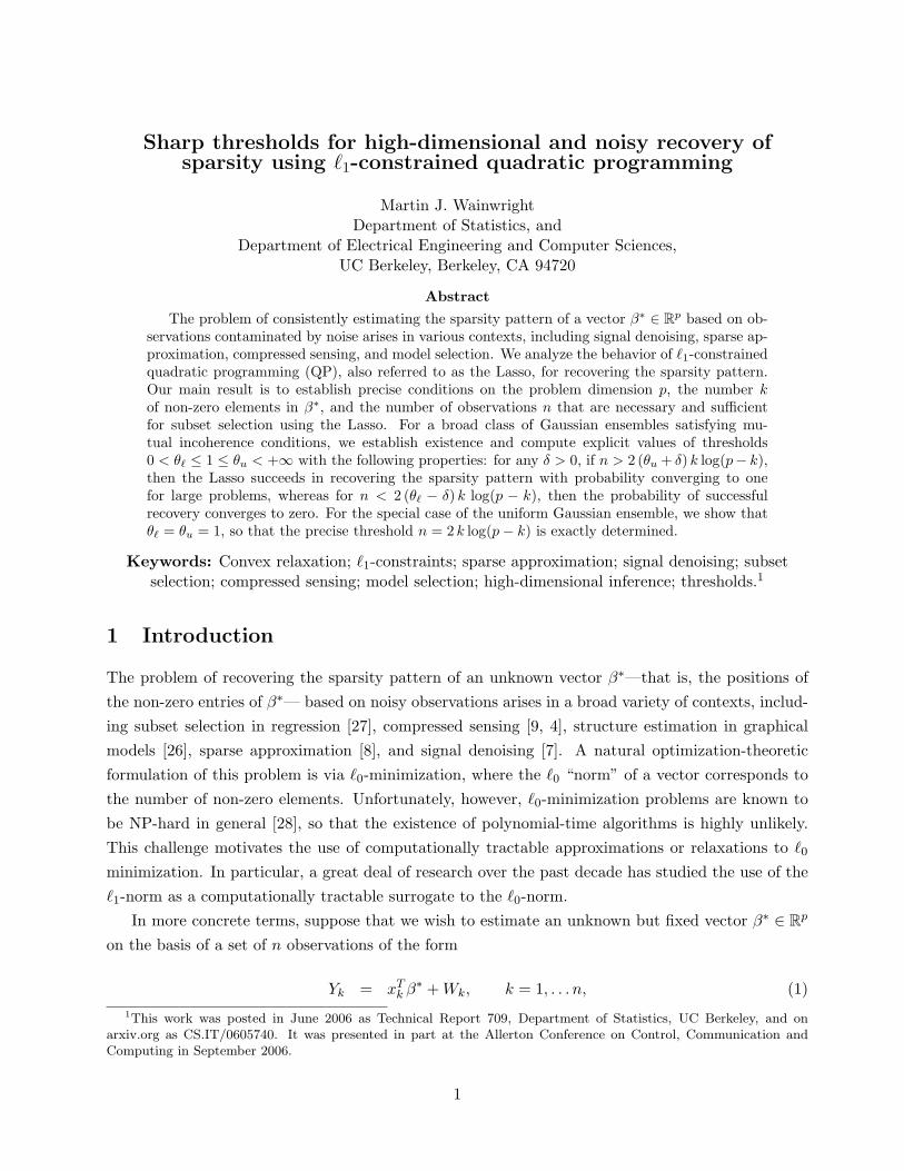
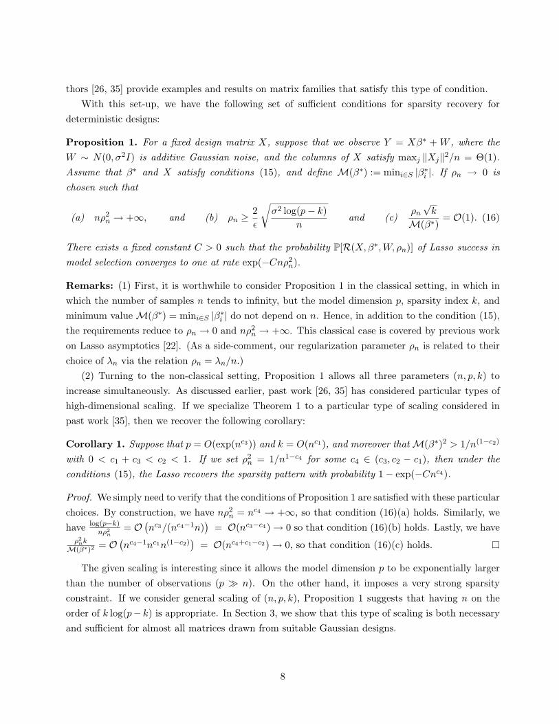
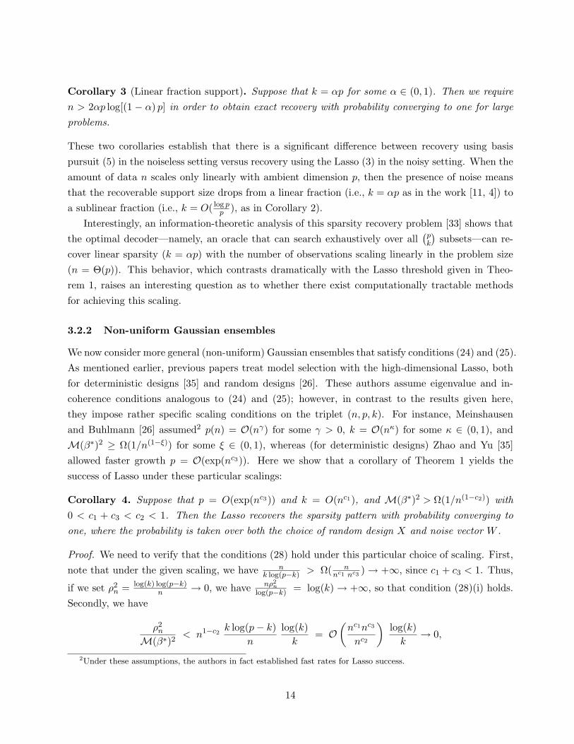
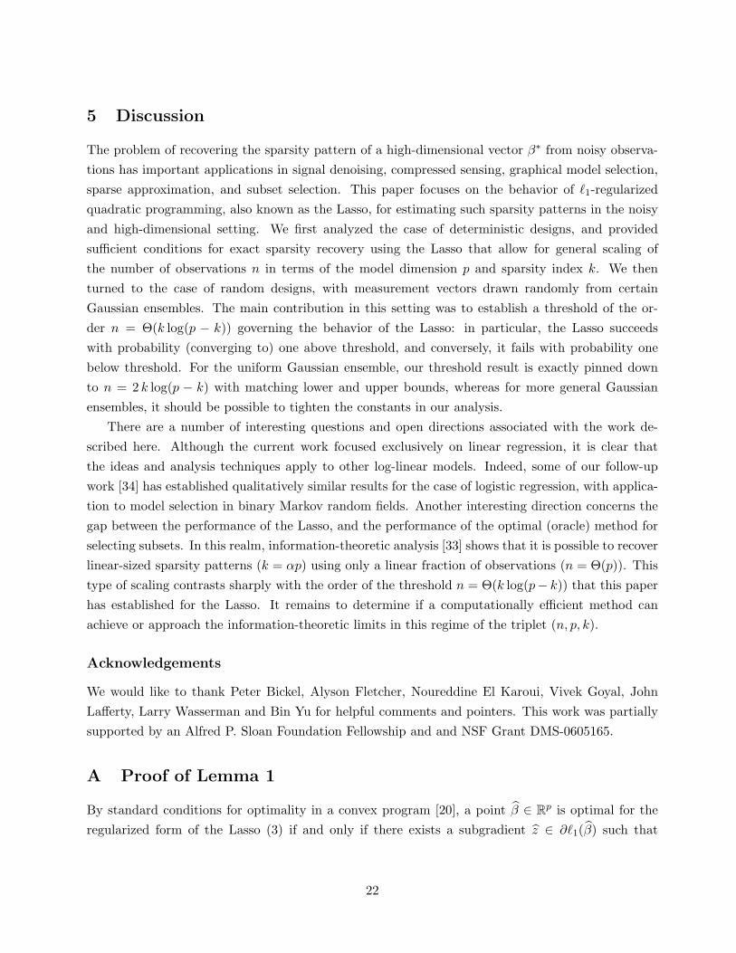
Figure 1. Plots of the number of data samples n = 2 θ k log(p− k), indexed by the control parameterθ, versus the probability of success in the Lasso for the uniform Gaussian ensemble. Each panel showsthree curves, corresponding to the problem sizes p ∈ 128, 256, 512, and each point on each curverepresents the average of 200 trials. (a) Linear sparsity index: k(p) = αp. (b) Sublinear sparsity indexk(p) = αp/ log(αp). (c) Fractional power sparsity index k(p) = αpγ with γ = 0.75. The thresholdin Lasso success probability occurs at θ∗ = 1, consistent with Theorem 1. See Section 4 for furtherdetails.

For the special case of the uniform Gaussian ensemble (i.e., xk ∼ N(0, Ip)) considered in past

work, we show that θℓ = θu = 1, so that the threshold is sharp. Figure 1 provides experimental

confirmation of the accuracy of this threshold behavior for finite-sized problems, with dimension p

ranging from 128 to 512. This threshold result has a number of connections to previous work in

the area that focuses on special forms of scaling. More specifically, as we discuss in more detail in

Section 3.2, in the special case of linear sparsity (i.e., k/p → α for some α > 0), this theorem provides

a noisy analog of results previously established for basis pursuit in the noiseless case [11, 4, 13].

5

Moreover, our result can also be adapted to an entirely different scaling regime, in which the sparsity

index is sublinear (k/p → 0), as considered by a separate body of recent work [26, 35] on the high-

dimensional Lasso.

The remainder of this paper is organized as follows. We begin in Section 2 with some necessary

and sufficient conditions, based on standard optimality conditions for convex programs, for property

R(X, β∗, W, ρn) to hold. We then prove a consistency result for the case of deterministic design

matrices X. Section 3 is devoted to the statement and proof of our main result on the asymptotic

behavior of the Lasso for random Gaussian ensembles. We illustrate this result via simulation in

Section 4, and conclude with a discussion in Section 5.

2 Preliminary analysis and deterministic designs

In this section, we provide necessary and sufficient conditions for Lasso to successfully recover the

sparsity pattern—or in shorthand, for property R(X, β∗, W, ρn) to hold. Based on these conditions,

we then define collections of random variables that play a central role in our analysis. In particular,

characterizing the event R(X, β∗, W, ρn) is reduced to studying the extreme order statistics of these

random variables. We then state and prove a result about the behavior of the Lasso for the case of

a deterministic design matrix X.

2.1 Convex optimality conditions

We begin with a simple set of necessary and sufficient conditions for property R(X, β∗, W, ρn) to

hold, which follow in a straightforward manner from optimality conditions for convex programs [20].

We define S := i ∈ 1, . . . , p | β∗i 6= 0 to be the support of β∗, and let Sc be its complement. For

any subset T ⊆ 1, 2, . . . , p, let XT be the n × |T | matrix with the vectors Xi, i ∈ T as columns.

Lemma 1. Assume that the matrix XTS XS is invertible. Then, for any given regularization parameter

ρ > 0 and noise vector w ∈ Rn, property R(X, β∗, w, ρ) holds if and only if

∣∣∣∣XTScXS

(XT

S XS

)−1[

1

nXT

S w − ρ sgn(β∗S)

]− 1

nXT

Scw

∣∣∣∣ ≤ ρ, and (10a)

sgn

β∗

S +

(1

nXT

S XS

)−1 [ 1

nXT

S w − ρ sgn(β∗S)

]= sgn(β∗

S), (10b)

where both of these vector relations should be taken elementwise. Moreover, if inequality (10a) holds

strictly, then any solution β of the Lasso (3) satisfies sgn(β) = sgn(β∗).

See Appendix A for the proof of this claim. For shorthand, define ~b := sgn(β∗S), and denote by

ei ∈ Rs the vector with 1 in the ith position, and zeroes elsewhere. Motivated by Lemma 1, much of

our analysis is based on the collections of random variables, defined each index i ∈ S and j ∈ Sc as

6

follows:

Ui := eTi

(1

nXT

S XS

)−1 [ 1

nXT

S W − ρn~b

](11a)

Vj := XTj

XS

(XT

S XS

)−1ρn

~b −[XS

(XT

S XS

)−1XT

S − In×n

]W

n

. (11b)

From Lemma 1, the behavior of R(X, β∗, W, ρn) is determined by the behavior of maxj∈Sc |Vj | and

maxi∈S |Ui|. In particular, condition (10a) holds if and only if the event

E(V ) :=

maxj∈Sc

|Vj | ≤ ρn

(12)

holds. On the other hand, if we define M(β∗) := mini∈S |β∗i |, then the event

E(U) :=

maxi∈S

|Ui| ≤ M(β∗)

(13)

is sufficient to guarantee that condition (10b) holds. Consequently, our proofs are based on analyzing

the asymptotic probability of these two events.

2.2 Recovery of sparsity: deterministic design

We now show how Lemma 1 can be used to analyze the behavior of the Lasso for the special

case of a deterministic (non-random) design matrix X. To gain intuition for the conditions in the

theorem statement, it is helpful to consider the zero-noise condition w = 0, in which each observation

Yk = xTk β∗ is uncorrupted. In this case, the conditions of Lemma 1 reduce to

∣∣∣XTScXS

(XT

S XS

)−1sgn(β∗

S)∣∣∣ ≤ 1 (14a)

sgn

(β∗

S − ρ

(1

nXT

S XS

)−1

sgn(β∗S)

)= sgn(β∗

S). (14b)

If the conditions of Lemma 1 fail to hold in the zero-noise setting, then there is little hope of

succeeding in the presence of noise. These zero-noise conditions motivate imposing the following set

of conditions on the design matrix:

∥∥∥XTScXS

(XT

S XS

)−1∥∥∥∞

≤ (1 − ǫ) for some ǫ ∈ (0, 1], and (15a)

λmin(1

nXT

S XS) ≥ Cmin > 0, (15b)

where λmin denotes the minimal eigenvalue. Mutual incoherence conditions of the form (15a) have

been considered in previous work on the Lasso, initially by Fuchs [17] and Tropp [32]. Other au-

7

thors [26, 35] provide examples and results on matrix families that satisfy this type of condition.

With this set-up, we have the following set of sufficient conditions for sparsity recovery for

deterministic designs:

Proposition 1. For a fixed design matrix X, suppose that we observe Y = Xβ∗ + W , where the

W ∼ N(0, σ2I) is additive Gaussian noise, and the columns of X satisfy maxj ‖Xj‖2/n = Θ(1).

Assume that β∗ and X satisfy conditions (15), and define M(β∗) := mini∈S |β∗i |. If ρn → 0 is

chosen such that

(a) nρ2n → +∞, and (b) ρn ≥ 2

ǫ

√σ2 log(p − k)

nand (c)

ρn

√k

M(β∗)= O(1). (16)

There exists a fixed constant C > 0 such that the probability P[R(X, β∗, W, ρn)] of Lasso success in

model selection converges to one at rate exp(−Cnρ2n).

Remarks: (1) First, it is worthwhile to consider Proposition 1 in the classical setting, in which in

which the number of samples n tends to infinity, but the model dimension p, sparsity index k, and

minimum value M(β∗) = mini∈S |β∗i | do not depend on n. Hence, in addition to the condition (15),

the requirements reduce to ρn → 0 and nρ2n → +∞. This classical case is covered by previous work

on Lasso asymptotics [22]. (As a side-comment, our regularization parameter ρn is related to their

choice of λn via the relation ρn = λn/n.)

(2) Turning to the non-classical setting, Proposition 1 allows all three parameters (n, p, k) to

increase simultaneously. As discussed earlier, past work [26, 35] has considered particular types of

high-dimensional scaling. If we specialize Theorem 1 to a particular type of scaling considered in

past work [35], then we recover the following corollary:

Corollary 1. Suppose that p = O(exp(nc3)) and k = O(nc1), and moreover that M(β∗)2 > 1/n(1−c2)

with 0 < c1 + c3 < c2 < 1. If we set ρ2n = 1/n1−c4 for some c4 ∈ (c3, c2 − c1), then under the

conditions (15), the Lasso recovers the sparsity pattern with probability 1 − exp(−Cnc4).

Proof. We simply need to verify that the conditions of Proposition 1 are satisfied with these particular

choices. By construction, we have nρ2n = nc4 → +∞, so that condition (16)(a) holds. Similarly, we

have log(p−k)nρ2

n= O

(nc3/(nc4−1n)

)= O(nc3−c4) → 0 so that condition (16)(b) holds. Lastly, we have

ρ2nk

M(β∗)2= O

(nc4−1nc1n(1−c2)

)= O(nc4+c1−c2) → 0, so that condition (16)(c) holds.

The given scaling is interesting since it allows the model dimension p to be exponentially larger

than the number of observations (p ≫ n). On the other hand, it imposes a very strong sparsity

constraint. If we consider general scaling of (n, p, k), Proposition 1 suggests that having n on the

order of k log(p− k) is appropriate. In Section 3, we show that this type of scaling is both necessary

and sufficient for almost all matrices drawn from suitable Gaussian designs.

8

2.3 Proof of Proposition 1

Recall the events E(V ) and E(U) defined in equations (12) and (13) respectively. To establish

the claim, we must show that that P[E(V )c or E(U)c] → 0, where E(V )c and E(U)c denote the

complements of these events. By union bound, it suffices to show both P[E(V )c] and P[E(U)c]

converge to zero, or equivalently that P[E(V )] and P[E(U)] both converge to one.

Analysis of E(V ): We begin by establishing that P[E(V )] → 1. Recalling our shorthand~b := sgn(β∗)

and the definition (11b) of the random variables Vj , note that E(V ) holds holds if and onlyminj∈Sc Vj

ρn≥

−1 andmaxj∈Sc Vj

ρn≤ 1. Moreover, we note that each Vj is Gaussian with mean µj = E[Vj ] =

ρnXTj XS

(XT

S XS

)−1~b . Using condition (15a), we have |µj | ≤ (1−ǫ) ρn for all indices j = 1, . . . , (p − k),

from which we obtain that

maxj∈Sc Vj

ρn≤ (1 − ǫ) +

1

ρnmax

jVj , and

minj∈Sc Vj

ρn≥ −(1 − ǫ) +

1

ρnmin

jVj ,

where Vj := XTj

[In×n − XS

(XT

S XS

)−1XT

S

]Wn

are zero-mean (correlated) Gaussian variables. Hence,

in order to establish condition (10a) of Lemma 1, we need to show that

P

[1

ρnminj∈Sc

Vj < −ǫ, or1

ρnmaxj∈Sc

Vj > ǫ

]→ 0. (17)

By symmetry (see Lemma 11 from Appendix C), it suffices to show that P[maxj∈Sc |eVj |

ρn> ǫ] → 0.

Using Gaussian comparison results [24] (see Lemma 9 in Appendix B), we haveE[maxj∈Sc |eVj |]

ρn≤

3√

log(p−k)

ρnmaxj

√E[V 2

j ]. Straightforward computation yields that

maxj

E[V 2j ] = max

j

σ2

n2XT

j

[In×n − XS

(XT

S XS

)−1XT

S

]Xj

≤ σ2

n2max

j‖Xj‖2 ≤ σ2

n,

since the projection matrix ΠS := In×n −XS

(XT

S XS

)−1XT

S has maximum eigenvalue equal to one,

and maxj ‖Xj‖22 ≤ n by assumption. Consequently, we have established that

E[maxj∈Sc

|Vj |] ≤√

σ2 log(p − k)

n

(i)

≤ ǫ ρn

2, (18)

where inequality (i) follows from condition (16)(b). We conclude the proof by claiming that for all

δ > 0, we have

P

[maxj∈Sc

|Vj | > E[maxj∈Sc

|Vj |] + δ

]≤ exp(−nδ2 σ2

2). (19)

9

To establish this claim, define a function f : Rn → R by f(w) = maxj∈Sc

∣∣∣∣σ2 XTj

nΠSw

∣∣∣∣. Note that by

construction, for a standard normal vector W ∼ N(0, In×n), we have f(W )d= maxj∈Sc |Vj |. Conse-

quently, the claim (19) will follow from measure concentration for Lipschitz functions of Gaussian

variates [23], as long as we can suitably upper bound the ℓ2-Lipschitz constant ‖f‖Lip. By the

triangle and Cauchy-Schwarz inequalities, we have

f(w) − f(v) ≤ maxj∈Sc

∣∣∣∣∣σ2XT

j

nΠS(w − v)

∣∣∣∣∣ = σ2 maxj∈Sc

‖Xj‖2

n‖ΠS‖2 ‖w − v‖2 =

σ2

√n‖w − v‖2,

since ‖ΠS‖2 = 1 and maxj ‖Xj‖2 ≤ √n by assumption. Hence, we have established that ‖f‖Lip ≤ σ2√

n

so that the concentration (19) follows.

Finally, if we set δ = ǫρn

2 , then we are guaranteed that δ + E[maxj∈Sc |Vj |] ≤ ρnǫ, so that

P

[maxj∈Sc |Vj | > ǫρn

]≤ exp(−nρ2

n ǫ2σ2

4 ) follows form the bound (19). Consequently, condition 16(a)

in the theorem statement—namely, that nρ2n → +∞—suffices to ensure that P(E(V )) → 1 at rate

exp(−Cnρ2n) as claimed.

Analysis of E(U): We now show that P(E(U)) → 1. Beginning with the triangle inequality, we

upper bound maxi∈S |Ui| := ‖( 1nXT

S XS)−1[ 1nXT

S W − ρn sgn(β∗S)]‖∞ as

maxi∈S

|Ui| ≤∥∥∥∥(

1

nXT

S XS)−1 1

nXT

S W

∥∥∥∥∞

+

∥∥∥∥(1

nXT

S XS)−1

∥∥∥∥∞

ρn (20)

The second term in this expansion is a deterministic quantity, which we bound as follows

ρn

∥∥∥∥(1

nXT

S XS)−1

∥∥∥∥∞

≤ ρn

√k λmax

((1

nXT

S XS)−1

)=

ρn

√k

λmin

(1nXT

S XS

) ≤ ρn

√k

Cmin, (21)

where we have use condition (15b) in the final step.

Turning to the first term in the expansion (20), let ei denote the unit vector with one in po-

sition i and zeroes elsewhere. Now define, for each index i ∈ S, the Gaussian random variable

Zi := eTi ( 1

nXT

S XS)−1 1nXT

S W . Each such Zi is a zero-mean Gaussian; computing its variance yields

var(Zi) = σ2

neTi ( 1

nXT

S XS)−1ei ≤ σ2

Cminn. Hence, by a standard Gaussian comparison theorem [24]

(in particular, see Lemma 9 in Appendix B), we have

E[maxi∈S

|Zi|] = E

[∥∥∥∥(1

nXT

S XS)−1 1

nXT

S W

∥∥∥∥∞

]≤ 3

√σ2 log k

nCmin. (22)

Now putting together the pieces, recall the definition M(β∗) := mini∈S |β∗i |. From the decom-

position (20) and the bound (21), order to have maxi∈S |Ui| ≤ M(β∗), it suffices to have ρn

√k

CminM(β∗)

be bounded above by constant (condition (16)(c)), which we may take equal to 12 by rescaling ρn as

10

necessary. With this deterministic term bounded, it suffices to have P[maxi∈S |Zi| > M(β∗)2 ] converge

to zero. To bound this probability, we first claim that for any δ > 0

P

[maxi∈S

|Zi| > E[maxi∈S

|Zi|] + δ

]≤ exp(−nδ2 σ2Cmin

2). (23)

As in the previous argument, this follows from concentration of measure for Lipschitz functions for

Gaussian random vectors, since ‖eTi ( 1

nXT

S XS)−1 1nXT

S ‖2 ≤ 1Cmin

√n.

Using the bound (22) and condition (16)(c), we have

E[maxi∈S |Zi|]M(β∗)

≤ 3

√σ2 log k

Cminn[M(β∗)]2= O

(√log k

Cminnρ2nk

)= O

(√1

nρ2n

),

which converges to zero using condition (16)(a) from the theorem statement. Hence, we may assume

that E[maxi∈S |Zi|] ≤ M(β∗)4 for sufficiently large n, and then take δ = M(β∗)

4 in the bound (23) to

conclude that

P[E(U)c] ≤ P

[maxi∈S

|Zi| >M(β∗)

2

]≤ exp(−nM(β∗)2 σ2Cmin

8) = O

(exp(−D

nρ2n σ2Cmin

8)

),

for some finite constant D, where the final inequality follows since ρ2n = O(M(β∗)2) from condi-

tion (16)(c). Thus, we have shown that P[E(U)] → 1 at rate exp(−Dnρ2n) for a suitable constant

D > 0 as claimed.

3 Recovery of sparsity: random Gaussian ensembles

The previous section treated the case of a deterministic design X, which allowed for a relatively

straightforward analysis. We now turn to the more complex case of random design matrices X,

in which each row xk is chosen as an i.i.d. Gaussian random vector with covariance matrix Σ. In

this setting, we provide precise conditions that govern the success and failure of the Lasso over this

ensemble; more specifically, we provide explicit thresholds that provide a sharp description of the

failure/success of the Lasso as a function of (n, p, k). We begin by setting up and providing a precise

statement of the main result, and then discussing its connections to previous work. In the later part

of this section, we provide the proof.

11

3.1 Statement of main result

Consider a covariance matrix Σ with unit diagonal, and with its minimum and maximum eigenvalues

(denoted λmin and λmax respectively) bounded as

λmin(ΣSS) ≥ Cmin, and λmax(Σ) ≤ Cmax (24)

for constants Cmin > 0 and Cmax < +∞. Given a vector β∗ ∈ Rp, define its support S = i ∈

1, . . . , p | β∗i 6= 0, as well as the complement Sc of its support. Suppose that Σ and S satisfy the

conditions ‖(ΣSS)−1‖∞ ≤ Dmax for some Dmax < +∞, and

‖ΣScS(ΣSS)−1‖∞ ≤ (1 − ǫ) (25)

for some ǫ ∈ (0, 1]. The simplest example of a covariance matrix satisfying these conditions is the

identity Σ = Ip×p, for which we have Cmin = Cmax = Dmax = 1, and ǫ = 1. Another well-known

matrix family satisfying these conditions are Toeplitz matrices (see Appendix D for details).

Under these conditions, we consider the observation model

Yk = xTk β∗ + Wk, k = 1, . . . , n, (26)

where xk ∼ N(0, Σ) and Wk ∼ N(0, σ2) are independent Gaussian variables for k = 1, . . . , n.

Furthermore, we define M(β∗) := mini∈S |β∗i |, and the sparsity index k = |S|.

Theorem 1. Consider a sequence of covariance matrices Σ[p] and solution vectors β∗[p] satisfy-

ing conditions (24) and (25). Under the observation model (26), consider a sequence (n, p(n), k(n))

such that k, (n − k) and (p − k) tend to infinity. Define the constants

θℓ :=(√

Cmax −√

Cmax − 1Cmax

)2

Cmax (2 − ǫ)2≤ 1, and θu :=

Cmax

ǫ2Cmin≥ 1. (27)

Then for any fixed δ > 0, we have the following

(a) If n < 2(θℓ − δ) k log(p− k), then P[R(X, β∗, W, ρn)] → 0 for any monotonic sequence ρn > 0.

(b) Conversely, if n > 2(θu + δ) k log(p − k), and ρn → 0 is chosen such that

(i)nρ2

n

log(p − k)→ +∞, and (ii)

ρn

M(β∗)= O(1) (28)

then P[R(X, β∗, W, ρn)] → 1.

Remark: Suppose for simplicity that M(β∗) remains bounded away from 0. In this case, the require-

ments on ρn reduce to ρn → 0, and ρ2nn/ log(p−k) → +∞. One suitable choice is ρ2

n = log(k) log(p−k)n

,

12

with which we have

ρ2n =

(k log(p − k)

n

)log(k)

k= O

(log k

k

)→ 0,

and nρ2n

log(p−k) = log(k) → +∞. More generally, under the threshold scaling of (n, p, k) given, the

theorem allows the minimum value M(β∗) := mini∈S |β∗i | to decay towards zero at rate Ω(1/

√k)

but not faster.

3.2 Some consequences

To develop intuition for this result, we begin by stating certain special cases as corollaries, and

discussing connections to previous work.

3.2.1 Uniform Gaussian ensembles

First, we consider the special case of the uniform Gaussian ensemble, in which Σ = Ip×p. Previous

work [4, 11] has focused on the uniform Gaussian ensemble in the the noiseless (σ2 = 0) and

underdetermined setting (n = γp for some γ ∈ (0, 1)). Analyzing the asymptotic behavior of the

linear program (5) for recovering β∗, the basic result is that there exists some α > 0 such that all

sparsity patterns with k ≤ αp can be recovered with high probability.

Applying Theorem 1 to the noisy version of this problem, the uniform Gaussian ensemble means

that we can choose ǫ = 1, and Cmin = Cmax = 1, so that the threshold constants reduce

θℓ =(√

Cmax −√

Cmax − 1Cmax

)2

Cmax (2 − ǫ)2= 1 and θu =

Cmax

ǫ2Cmin= 1.

Consequently, Theorem 1 provides a sharp threshold for the behavior of the Lasso, in that fail-

ure/success is entirely determined by whether or not n > 2k log(p − k). Thus, if we consider the

linear scaling n = Θ(p) analyzed in previous work on the noiseless case [11, 4], we have:

Corollary 2 (Linearly underdetermined setting). Suppose that n = γp for some γ ∈ (0, 1). Then

(a) If k = αp for any α ∈ (0, 1), then P [R(X, β∗, W, ρn)] → 0 for any positive sequence ρn > 0.

(b) On the other hand, if k = O( plog p

), then P [R(X, β∗, W, ρn)] → 1 for any sequence ρn satis-

fying the conditions of Theorem 1(a).

Conversely, suppose that the size k of the support of β∗ scales linearly with the number of parameters

p. The following result describes the amount of data required for the ℓ1-constrained QP to recover

the sparsity pattern in the noisy setting (σ2 > 0):

13

Corollary 3 (Linear fraction support). Suppose that k = αp for some α ∈ (0, 1). Then we require

n > 2αp log[(1 − α) p] in order to obtain exact recovery with probability converging to one for large

problems.

These two corollaries establish that there is a significant difference between recovery using basis

pursuit (5) in the noiseless setting versus recovery using the Lasso (3) in the noisy setting. When the

amount of data n scales only linearly with ambient dimension p, then the presence of noise means

that the recoverable support size drops from a linear fraction (i.e., k = αp as in the work [11, 4]) to

a sublinear fraction (i.e., k = O( log pp

), as in Corollary 2).

Interestingly, an information-theoretic analysis of this sparsity recovery problem [33] shows that

the optimal decoder—namely, an oracle that can search exhaustively over all(pk

)subsets—can re-

cover linear sparsity (k = αp) with the number of observations scaling linearly in the problem size

(n = Θ(p)). This behavior, which contrasts dramatically with the Lasso threshold given in Theo-

rem 1, raises an interesting question as to whether there exist computationally tractable methods

for achieving this scaling.

3.2.2 Non-uniform Gaussian ensembles

We now consider more general (non-uniform) Gaussian ensembles that satisfy conditions (24) and (25).

As mentioned earlier, previous papers treat model selection with the high-dimensional Lasso, both

for deterministic designs [35] and random designs [26]. These authors assume eigenvalue and in-

coherence conditions analogous to (24) and (25); however, in contrast to the results given here,

they impose rather specific scaling conditions on the triplet (n, p, k). For instance, Meinshausen

and Buhlmann [26] assumed2 p(n) = O(nγ) for some γ > 0, k = O(nκ) for some κ ∈ (0, 1), and

M(β∗)2 ≥ Ω(1/n(1−ξ)) for some ξ ∈ (0, 1), whereas (for deterministic designs) Zhao and Yu [35]

allowed faster growth p = O(exp(nc3)). Here we show that a corollary of Theorem 1 yields the

success of Lasso under these particular scalings:

Corollary 4. Suppose that p = O(exp(nc3)) and k = O(nc1), and M(β∗)2 > Ω(1/n(1−c2)) with

0 < c1 + c3 < c2 < 1. Then the Lasso recovers the sparsity pattern with probability converging to

one, where the probability is taken over both the choice of random design X and noise vector W .

Proof. We need to verify that the conditions (28) hold under this particular choice of scaling. First,

note that under the given scaling, we have nk log(p−k) > Ω( n

nc1 nc3) → +∞, since c1 + c3 < 1. Thus,

if we set ρ2n = log(k) log(p−k)

n→ 0, we have nρ2

n

log(p−k) = log(k) → +∞, so that condition (28)(i) holds.

Secondly, we have

ρ2n

M(β∗)2< n1−c2

k log(p − k)

n

log(k)

k= O

(nc1nc3

nc2

)log(k)

k→ 0,

2Under these assumptions, the authors in fact established fast rates for Lasso success.

14

since c1 + c3 − c2 < 0, which shows that condition (28)(ii) holds strongly.

3.3 Proof of Theorem 1(b)

We now turn to the proof of part (b) of our main result. As with the proof of Proposition 1, the

proof is based on analyzing the collections of random variables Vj | j ∈ Sc and Ui | i ∈ S,as defined in equations (11a) and (11b) respectively. We begin with some preliminary results that

serve to set up the argument.

3.3.1 Some preliminary results

We first note that for k < n, the random Gaussian matrix XS will have rank k with probability

one, whence the matrix XTS XS is invertible with probability one. Accordingly, the necessary and

sufficient conditions of Lemma 1 are applicable. Our first lemma, proved in Appendix E.1, concerns

the behavior of the random vector V = (V1, . . . , V(p−k)), when conditioned on XS and W . Recalling

the shorthand notation ~b := sgn(β∗), we summarize in the following

Lemma 2. Conditioned on XS and W , the random vector (V | W, XS) is Gaussian. Its mean

vector is upper bounded as

|E[V | W, XS ]| ≤ ρn(1 − ǫ)1. (29)

Moreover, its conditional covariance takes the form

cov[V | W, XS ] = MnΣ(Sc |S) = Mn

[ΣScSc − ΣScS(ΣSS)−1ΣSSc

], (30)

where

Mn := ρ2n~b T (XT

S XS)−1~b +1

n2W T

[In×n − XS

(XT

S XS

)−1XT

S

]W (31)

is a random scaling factor.

The following lemma, proved in Appendix E.2, captures the behavior of the random scaling factor

Mn defined in equation (31):

Lemma 3. The random variable Mn has mean

E[Mn] =ρ2

n

n − k − 1~b T (ΣSS)−1~b +

σ2 (n − k)

n2. (32)

Moreover, it is concentrated: for any δ > 0, we have P[∣∣Mn − E[Mn]

∣∣ ≥ δE[Mn]]→ 0 as n → +∞.

15

3.3.2 Main argument

With these preliminary results in hand, we now turn to analysis of the collections of random variables

Ui, i ∈ S and Vj , j ∈ Sc.

Analysis of E(V ): We begin by analyzing the behavior of maxj∈Sc |Vj |. First, for a fixed but

arbitrary δ > 0, define the event T (δ) := |Mn − E[Mn]| ≥ δE[Mn]. By conditioning on T (δ) and

its complement [T (δ)]c, we have the upper bound

P[maxj∈Sc

|Vj | > ρn] ≤ P

[maxj∈Sc

|Vj | > ρn | [T (δ)]c]

+ P[T (δ)].

By the concentration statement in Lemma 3, we have P[T (δ)] → 0, so that it suffices to analyze

the first term. Set µj = E[Vj |XS ], and let Z be a zero-mean Gaussian vector with cov(Z) =

cov(V |XS , W ). We then have

maxj∈Sc

|Vj | = maxj∈Sc

|µj + Zj |

≤ (1 − ǫ)ρn + maxj∈Sc

|Zj |,

where we have used the triangle inequality, and the upper bound (29) on the mean. This inequality

establishes the inclusion of events maxj∈Sc |Zj | ≤ ǫρn ⊆ maxj∈Sc |Vj | ≤ ρn, thereby showing

that it suffices to prove that P[maxj∈Sc |Zj | > ǫρn | [T (δ)]c] → 0.

Note that conditioned on [T (δ)]c, the maximum value of Mn is M∗n := (1 + δ)E[Mn]. Since

Gaussian maxima increase with increasing variance, we have

P

[maxj∈Sc

|Zj | > ǫρn | [T (δ)]c]

≤ P

[maxj∈Sc

|Zj | > ǫρn

],

where Z is zero-mean Gaussian with covariance M∗n Σ(Sc|S).

Using Lemma 11, it suffices to show that P[maxj∈Sc Zj > ǫρn] converges to zero. Accordingly, we

complete this part of the proof via the following two lemmas, both of which are proved in Appendix E:

Lemma 4. Under the stated assumptions of the theorem, we have M∗n

ρ2n

→ 0 and

limn→+∞

1

ρnE[max

j∈ScZj ] ≤ ǫ.

Lemma 5. For any η > 0, we have

P

[maxj∈Sc

Zj > η + E[maxj∈Sc

Zj ]

]≤ exp

(− η2

2M∗n

). (33)

Lemma 4 implies that for all δ > 0, we have E[maxj∈Sc Zj ] ≤ (1 + δ2)ǫρn for all n sufficiently

16

large. Therefore, setting η = δ2ρnǫ in the bound (33), we have for fixed δ > 0 and n sufficiently large:

P

[maxj∈Sc

Zj > (1 + δ)ρnǫ

]≤ P

[maxj∈Sc

Zj >δ

2ρnǫ + E[max

j∈ScZj ]

]

≤ 2 exp

(−δ2ρ2

nǫ2

8M∗n

).

From Lemma 4, we have ρ2n/M∗

n → +∞, which implies that P[maxj∈Sc Zj > (1 + δ)ρnǫ] → 0 for all

δ > 0. By the arbitrariness of δ > 0, we thus have P[maxj∈Sc Zj ≤ ǫρn] → 1, thereby establishing

that property (10a) of Lemma 1 holds w.p. one asymptotically.

Analysis of E(U): Next we prove that maxi∈S |Ui| < M(β∗) := mini∈S |β∗i | with probability one

as n → +∞. Conditioned on XS , the only random component in Ui is the noise vector W . A

straightforward calculation yields that this conditioned RV is Gaussian, with mean and variance

Yi := E[Ui | XS ] = −ρneTi

(1

nXT

S XS

)−1~b ,

Y ′i := var[Ui | XS ] =

σ2

neTi

[1

nXT

S XS

]−1

ei,

respectively. The following lemma, proved in Appendix E.5, is key to our proof:

Lemma 6. (a) The random variables Yi and Y ′i have means

E[Yi] =−ρn n

n − k − 1eTi (ΣSS)−1~b , and E[Y ′

i ] =σ2

n − k − 1eTi (ΣSS)−1ei, (34)

respectively, which are bounded as

|E[Yi]| ≤ 2Dmaxnρn

n − k − 1, and

σ2

Cmax (n − k − 1)≤ E[Y ′

i ] ≤ σ2Dmax

n − k − 1. (35)

(b) Moreover, each pair (Yi, Y′i ) is concentrated, in that we have

P

[|Yi| ≥

6Dmaxnρn

n − k − 1, or |Y ′

i | ≥ 2E[Y ′i ]

]= O

(1

n − k

). (36)

We exploit this lemma as follows. First define the event

T (δ) :=k⋃

i=1

|Yi| ≥

6Dmaxnρn

n − k − 1, or |Y ′

i | ≥ 2E[Y ′i ]

.

By the union bound and Lemma 6(b), we have P[T (δ)] = O(k 1

n−k

)= O

(1

nk−1

)→ 0, since

17

nk→ +∞ as n → +∞ under the scaling n > Ω(k log(p − k)). For convenience in notation, for any

a ∈ R and b ∈ R+, we use Ui(a, b) to denote a Gaussian random variable with mean a and variance

b. Conditioning on the event T (δ) and its complement, we have

P[maxi∈S

|Ui| > M(β∗)] ≤ P[maxi∈S

|Ui| > M(β∗) | T (δ)c] + P[T (δ)]

≤ P[maxi∈S

|Ui(µ∗i , ν(i))| > M(β∗)] + O

(1

nk− 1

), (37)

where each Ui(µ∗i , M

∗i ) is Gaussian with mean µ∗

i := 6Dmaxρnn

n−k−1 and variance νi := 2E[Y ′i ]

respectively. In asserting the inequality (37), we have used the fact that the probability of the event

Ui > M(β∗) increases as the mean and variance of Ui increase. Continuing the argument assuming

the conditioning on T (δ)c, we have via

P[1

M(β∗)maxi∈S

|Ui(µ∗i , νi)| > 1] ≤ P

[1

M(β∗)maxi∈S

|Ui(0, νi)| > 1 − maxi∈S |µ∗i |

M(β∗)

]

(i)

≤ P

[1

M(β∗)maxi∈S

|Ui(0, νi)| > 1 − 2Dmaxnρn

(n − k − 1)M(β∗)

]

≤ P

[1

M(β∗)maxi∈S

|Ui(0, νi)| > 1 − 2Dmaxρn

M(β∗)

]

(ii)

≤ P

[1

M(β∗)maxi∈S

|Ui(0, νi)| >1

2

],

where inequality (i) uses the conditioning on T (δ)c and Lemma 6(b), and inequality (ii) uses condition

(b) on ρn in the theorem statement.

Next we use Markov’s inequality, the bound (35) on νi := 2E[Y ′i ], and Lemma 9 on Gaussian

maxima (see Appendix B) to obtain the upper bound

P

[1

M(β∗)maxi∈S

|Ui(0, νi)| >1

2

]≤ 2E[maxi∈S |Ui(0, M∗

i )|]M(β∗)

≤ 6

M(β∗)

√2σ2 Dmax log k

n − k − 1.

Finally, using condition (ii) in equation (28), we have log kM(β∗)2 (n−k−1)

≤ log kρ2

n (n−k−1)= O( log(p−k)

ρ2n n

),

which converges to zero from condition (28)(i) in the theorem statement.

3.4 Proof of Theorem 1(a)

We establish the claim by proving that under the stated conditions, maxj∈Sc |Vj | > ρn with prob-

ability one, for any positive sequence ρn > 0. We begin by writing Vj = E[Vj ] + Vj , where Vj is

18

zero-mean. Now

maxj∈Sc

|Vj | ≥ maxj∈Sc

|Vj | − maxj∈Sc

|E[Vj ]|(i)

≥ maxj∈Sc

|Vj | − (1 − ǫ)ρn,

where have used Lemma 2 in obtaining the lower bound (i). Consequently, the event maxj∈Sc |Vj | >

(2 − ǫ)ρn implies the event maxj∈Sc |Vj | > ρn, so that

P[maxj∈Sc

|Vj | > ρn] ≥ P[maxj∈Sc

|Vj | > (2 − ǫ) ρn].

From the preceding proof of Theorem 1(b), we know that conditioned on XS and W , the random

vector (V1, . . . , V(p−k)) is Gaussian with covariance of the form Mn [ΣScSc −ΣScS(ΣSS)−1ΣSSc ]; thus,

the zero-mean version (V1, . . . , V(p−k)) has the same covariance. Moreover, Lemma 3 guarantees

that the random scaling term Mn is concentrated. In particular, defining for any δ > 0 the event

T (δ) := |Mn − E[Mn]| ≥ δE[Mn], we have P[T (δ)] → 0, and the bound

P[maxj∈Sc

|Vj | > (2 − ǫ) ρn] ≥ (1 − P[T (δ)]) P

[maxj∈Sc

|Vj | > (2 − ǫ) ρn | T (δ)c

]

(ii)

≥ (1 − P[T (δ)]) P

[maxj∈Sc

|Zj(M∗n)| > (2 − ǫ) ρn

],

where each Zj ≡ Zj(M∗n) is the conditioned version of Vj with the scaling factor Mn fixed to

M∗n := (1 − δ)E[Mn]. (In inequality (ii) above, we used the fact that Gaussian tail probabilities

decrease as the variance decreases, and the fact that var(Vj) ≥ M∗n when conditioned on T (δ)c.)

Our proof proceeds by first analyzing the expected value, and then exploiting Gaussian concen-

tration of measure for Lipschitz functions. We summarize the key results in the following:

Lemma 7. Under the stated conditions, one of the following two conditions must hold:

(a) either ρ2n

M∗n→ +∞, and there exists some γ > 0 such that 1

ρnE[maxj∈Sc Zj ] ≥ (2− ǫ) [1 + γ] for

all sufficiently large n, or

(b) there exist constants α, γ > 0 such that M∗n

ρ2n

≤ α and 1ρn

E[maxj∈Sc Zj ] ≥ γ√

log (p − k) for all

sufficiently large n.

Lemma 8. For any η > 0, we have

P[maxj∈Sc

Zj(M∗n) < E[max

j∈ScZj(M

∗n)] − η] ≤ exp

(− η2

2M∗n

). (38)

Using these two lemmas, we complete the proof as follows. First, if condition (a) of Lemma 7

19

holds, then we set η = (2−ǫ) γρn

2 in equation (38) to obtain that

P[1

ρnmaxj∈Sc

Zj(M∗n) ≥ (2 − ǫ) (1 +

γ

2) ] ≥ 1 − exp

(−(2 − ǫ)2 γ2ρ2

n

8M∗n

).

This probability converges to 1 since ρ2n

M∗n→ +∞ from Lemma 7(a). On the other hand, if condition

(b) holds, then we use the bound 1ρn

E[maxj∈Sc Zj ] ≥ γ√

log (p − k) and set η =γρn

√log (p−k)

2 in

equation (38) to obtain

P[1

ρnmaxj∈Sc

Zj(M∗n) > 2 (2 − ǫ) ] ≥ P[

1

ρnmaxj∈Sc

Zj(M∗n) ≥ γ

√log (p − k)

2]

≥ 1 − exp

(−γ2ρ2

n log (p − k)

8M∗n

).

This probability also converges to 1 since ρ2n

M∗n≥ 1/α and log (p − k) → +∞. Thus, in either case,

we have shown that limn→+∞ P[ 1ρn

maxj∈Sc Zj(M∗n) > (2 − ǫ)] = 1, thereby completing the proof of

Theorem 1(a).

4 Illustrative simulations

In this section, we provide some simulations to confirm the threshold behavior predicted by Theo-

rem 1. We consider the following three types of sparsity indices:

(a) linear sparsity, meaning that k(p) = αp for some α ∈ (0, 1);

(b) sublinear sparsity, meaning that k(p) = αp/(log(αp)) for some α ∈ (0, 1), and

(c) fractional power sparsity, meaning that k(p) = αpγ for some α, γ ∈ (0, 1).

For all three types of sparsity indices, we investigate the success/failure of the Lasso in recovering

the sparsity pattern, where the number of observations scales as n = 2 θ k log(p − k) + k + 1. The

control parameter θ is varied in the interval (0, 2.4). For all results shown here, we fixed α = 0.40 for

all three ensembles, and set γ = 0.75 for the fractional power ensemble. We specified the parameter

vector β∗ by choosing the subset S randomly, and for each i ∈ S setting β∗i equal to +1 or −1 with

equal probability, and β∗j = 0 for all indices j /∈ S. In addition, we fixed the noise level σ = 0.5, and

the regularization parameter ρn =

√log(p−k) log(k)

nin all cases.

We begin by considering the uniform Gaussian ensemble, in which each row xk is chosen in an

i.i.d. manner from the multivariate N(0, Ip×p) distribution. Recall that for the uniform Gaussian

ensemble, the critical value is θu = θℓ = 1. Figure 1, displayed earlier in Section 1, plots the control

parameter θ versus the probability of success, for linear sparsity (a), sublinear sparsity pattern (b),

and fractional power sparsity (c), for three different problem sizes (p ∈ 128, 256, 512). Each point

20

represents the average of 200 trials. Note how the probability of success rises rapidly from 0 around

the predicted threshold point θ = 1, with the sharpness of the threshold increasing for larger problem

sizes.

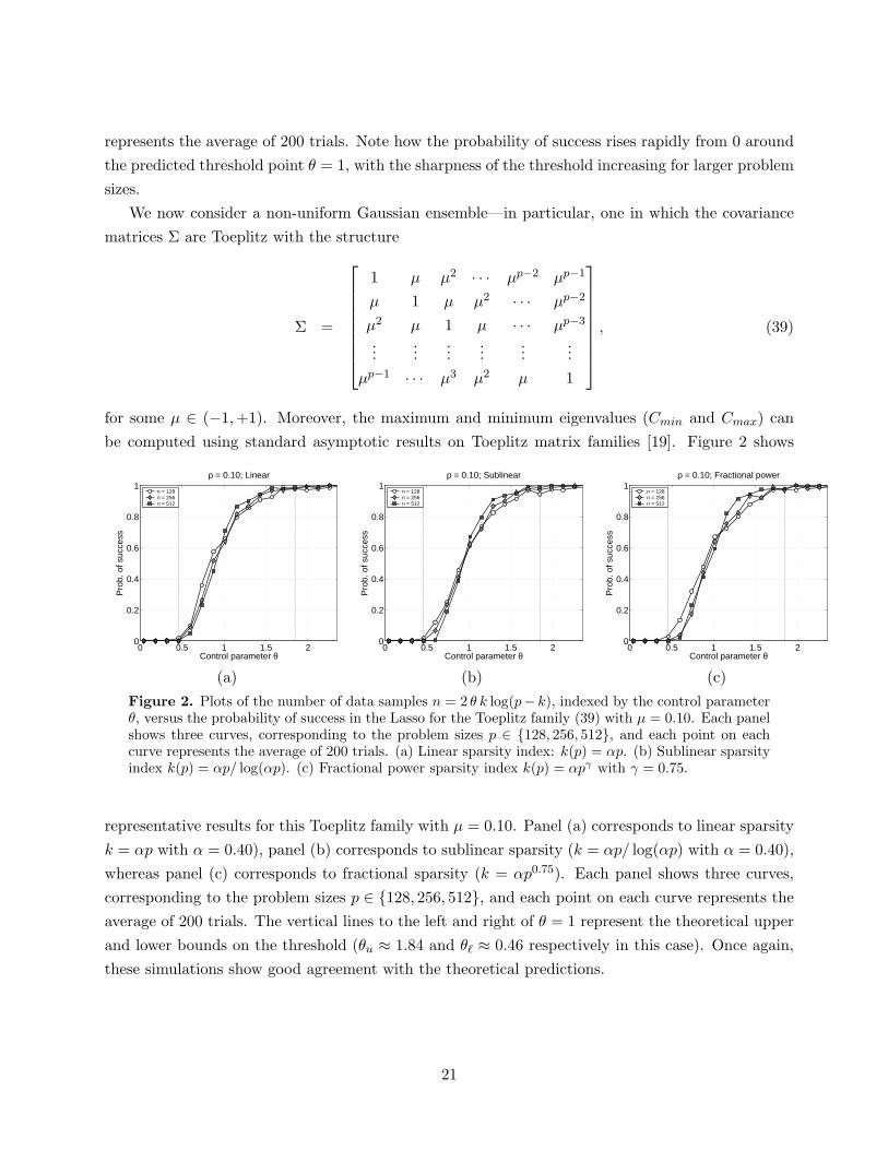
We now consider a non-uniform Gaussian ensemble—in particular, one in which the covariance

matrices Σ are Toeplitz with the structure

Σ =

1 µ µ2 · · · µp−2 µp−1

µ 1 µ µ2 · · · µp−2

µ2 µ 1 µ · · · µp−3

......

......

......

µp−1 · · · µ3 µ2 µ 1

, (39)

for some µ ∈ (−1, +1). Moreover, the maximum and minimum eigenvalues (Cmin and Cmax) can

be computed using standard asymptotic results on Toeplitz matrix families [19]. Figure 2 shows

0 0.5 1 1.5 20

0.2

0.4

0.6

0.8

1

Control parameter θ

Pro

b. o

f suc

cess

ρ = 0.10; Linear

n = 128n = 256n = 512

0 0.5 1 1.5 20

0.2

0.4

0.6

0.8

1

Control parameter θ

Pro

b. o

f suc

cess

ρ = 0.10; Sublinear

n = 128n = 256n = 512

0 0.5 1 1.5 20

0.2

0.4

0.6

0.8

1

Control parameter θ

Pro

b. o

f suc

cess

ρ = 0.10; Fractional power

n = 128n = 256n = 512

(a) (b) (c)

Figure 2. Plots of the number of data samples n = 2 θ k log(p− k), indexed by the control parameterθ, versus the probability of success in the Lasso for the Toeplitz family (39) with µ = 0.10. Each panelshows three curves, corresponding to the problem sizes p ∈ 128, 256, 512, and each point on eachcurve represents the average of 200 trials. (a) Linear sparsity index: k(p) = αp. (b) Sublinear sparsityindex k(p) = αp/ log(αp). (c) Fractional power sparsity index k(p) = αpγ with γ = 0.75.

representative results for this Toeplitz family with µ = 0.10. Panel (a) corresponds to linear sparsity

k = αp with α = 0.40), panel (b) corresponds to sublinear sparsity (k = αp/ log(αp) with α = 0.40),

whereas panel (c) corresponds to fractional sparsity (k = αp0.75). Each panel shows three curves,

corresponding to the problem sizes p ∈ 128, 256, 512, and each point on each curve represents the

average of 200 trials. The vertical lines to the left and right of θ = 1 represent the theoretical upper

and lower bounds on the threshold (θu ≈ 1.84 and θℓ ≈ 0.46 respectively in this case). Once again,

these simulations show good agreement with the theoretical predictions.

21

5 Discussion

The problem of recovering the sparsity pattern of a high-dimensional vector β∗ from noisy observa-

tions has important applications in signal denoising, compressed sensing, graphical model selection,

sparse approximation, and subset selection. This paper focuses on the behavior of ℓ1-regularized

quadratic programming, also known as the Lasso, for estimating such sparsity patterns in the noisy

and high-dimensional setting. We first analyzed the case of deterministic designs, and provided

sufficient conditions for exact sparsity recovery using the Lasso that allow for general scaling of

the number of observations n in terms of the model dimension p and sparsity index k. We then

turned to the case of random designs, with measurement vectors drawn randomly from certain

Gaussian ensembles. The main contribution in this setting was to establish a threshold of the or-

der n = Θ(k log(p − k)) governing the behavior of the Lasso: in particular, the Lasso succeeds

with probability (converging to) one above threshold, and conversely, it fails with probability one

below threshold. For the uniform Gaussian ensemble, our threshold result is exactly pinned down

to n = 2 k log(p − k) with matching lower and upper bounds, whereas for more general Gaussian

ensembles, it should be possible to tighten the constants in our analysis.

There are a number of interesting questions and open directions associated with the work de-

scribed here. Although the current work focused exclusively on linear regression, it is clear that

the ideas and analysis techniques apply to other log-linear models. Indeed, some of our follow-up

work [34] has established qualitatively similar results for the case of logistic regression, with applica-

tion to model selection in binary Markov random fields. Another interesting direction concerns the

gap between the performance of the Lasso, and the performance of the optimal (oracle) method for

selecting subsets. In this realm, information-theoretic analysis [33] shows that it is possible to recover

linear-sized sparsity patterns (k = αp) using only a linear fraction of observations (n = Θ(p)). This

type of scaling contrasts sharply with the order of the threshold n = Θ(k log(p− k)) that this paper

has established for the Lasso. It remains to determine if a computationally efficient method can

achieve or approach the information-theoretic limits in this regime of the triplet (n, p, k).

Acknowledgements

We would like to thank Peter Bickel, Alyson Fletcher, Noureddine El Karoui, Vivek Goyal, John

Lafferty, Larry Wasserman and Bin Yu for helpful comments and pointers. This work was partially

supported by an Alfred P. Sloan Foundation Fellowship and and NSF Grant DMS-0605165.

A Proof of Lemma 1

By standard conditions for optimality in a convex program [20], a point β ∈ Rp is optimal for the

regularized form of the Lasso (3) if and only if there exists a subgradient z ∈ ∂ℓ1(β) such that

22

1nXT Xβ − 1

nXT y + ρz = 0. Here the subdifferential of the ℓ1 norm takes the form

∂ℓ1(β) =

z ∈ Rp | zi = sgn(βi) for βi 6= 0, |zj | ≤ 1 otherwise

. (40)

Substituting our observation model y = Xβ∗ + w and re-arranging yields

1

nXT X(β − β∗) − 1

nXT w + ρz = 0. (41)

Now condition R(X, β∗, w, ρ) holds if and only if β satisfies βSc = 0 and βS 6= 0, and the subgradient

satisfies zS = sgn(β∗S) and |zSc | ≤ 1. From these conditions and using equation (41), we conclude

that the condition R(X, β∗, w, ρ) holds if and only if

1

nXT

ScXS

(βS − β∗

S

)− 1

nXT

Scw = −ρzSc .

1

nXT

S XS

(βS − β∗

S

)− 1

nXT

S w = −ρ sgn(β∗S).

Using the invertibility of XTS XS , we may solve for βS and zSc to conclude that

ρ zSc = XTScXS

(XT

S XS

)−1[

1

nXT

S w − ρ sgn(β∗S)

]− 1

nXT

Scw

βS = β∗S +

(1

nXT

S XS

)−1 [ 1

nXT

S w − ρ sgn(β∗S)

].

From these relations, the requirements |zSc | ≤ 1 and sgn(βS) = sgn(β∗S) yield conditions (10a)

and (10b) respectively. Lastly, note that if the vector inequality |zSc | < 1 holds strictly, then βSc = 0

for all solutions to the Lasso as claimed.

B Some Gaussian comparison results

We state here (without proof) some well-known comparison results on Gaussian maxima [24]. We

begin with a crude but useful bound:

Lemma 9. For any Gaussian RV (X1, . . . , Xn), E[ max1≤i≤n

|Xi|] ≤ 3√

log n max1≤i≤n

√EX2

i .

Next we state (a version of) the Sudakov-Fernique inequality [24]:

Lemma 10 (Sudakov-Fernique). Let X = (X1, . . . , Xn) and Y = (Y1, . . . , Yn) be Gaussian random

vectors such that for all i, j E[(Yi − Yj)2] ≤ E[(Xi − Xj)

2]. Then E[ max1≤i≤n

Yi] ≤ E[ max1≤i≤n

Xi].

C Auxiliary lemma

For future use, we state formally the following elementary

23

Lemma 11. Given a collection Z1, Z2, . . . , Z(p−k) of random variables with distribution symmetric

around zero, for any constant a > 0 we have

P[ max1≤j≤(p−k)

|Zj | ≤ a] ≤ P[ max1≤j≤(p−k)

Zj ≤ a], and (44a)

P[ max1≤j≤(p−k)

|Zj | > a] ≤ 2P[ max1≤j≤(p−k)

Zj > a]. (44b)

Proof. The first inequality is trivial. To establish the inequality (44b), we write

P[ max1≤j≤(p−k)

|Zj | > a] = P[( max1≤j≤(p−k)

Zj > a) or ( min1≤j≤(p−k)

Zj < −a)]

≤ P[ max1≤j≤(p−k)

Zj > a] + P[ min1≤j≤(p−k)

Zj < −a]

= 2P[ max1≤j≤(p−k)

Zj > a],

where we have used the union bound, and the symmetry of the events max1≤j≤(p−k) Zj > a and

min1≤j≤(p−k) Zj < −a.

D Toeplitz covariance matrices

In this appendix, we verify that Toeplitz covariance matrices satisfy the conditions of Theorem 1.

Standard results on Toeplitz matrices [19] show that the eigenvalues are suitably bounded. Previous

work [35] has shown that Toeplitz families satisfy the mutual incoherence condition (25). It remains

to verify the bound ‖(ΣSS)−1‖∞ ≤ Dmax. From the block matrix inversion formula [21], we have

(ΣSS)−1 = (Σ−1)SS − (Σ−1)SSc

[(Σ−1)ScSc

]−1(Σ−1)ScS . Applying the triangle inequality yields

‖(ΣSS)−1‖∞ ≤ ‖(Σ−1)SS‖∞ + ‖(Σ−1)SSc‖∞ ‖[(Σ−1)ScSc

]−1 ‖∞ ‖(Σ−1)ScS‖∞ (45)

For a Toeplitz matrix Σ = toep[1 µ . . . µp−1], the inverse is tridiagonal with bounded diagonal

entries ai(µ), immediate off-diagonals bij(µ), and all other entries equal to zero. Hence, it follows

immediately that the matrix norms ‖(Σ−1)SS |∞, ‖(Σ−1)SSc‖∞, and ‖(Σ−1)ScS‖∞ are all bounded

(independently of k and p). Finally, the matrix (Σ−1)ScSc is blockwise tridiagonal, with each block

corresponding to a subset of indices T ⊆ Sc all connected by single hops. Hence, the inverse matrix[(Σ−1)ScSc

]−1is a blockwise Toeplitz matrix. Each block can be interpreted as the covariance matrix

of a stable autoregressive process, so that the ℓ∞ norm of each row is bounded independently of p

and the choice of Sc. Thus, we conclude that ‖[(Σ−1)ScSc

]−1 ‖∞ is upper bounded independently

of p and Sc, and hence via equation (45) that the same holds for ‖(ΣSS)−1‖∞ as claimed.

24

E Lemma for Theorem 1

E.1 Proof of Lemma 2

Conditioned on both XS and W , the only random component in Vj is the column vector Xj . Using

standard LLSE formula [2] (i.e., for estimating XSc on the basis of XS), the random variable (XSc |XS , W ) ∼ (XSc | XS) is Gaussian with mean and covariance

E[XTSc | XS , W ] = ΣScS(ΣSS)−1XT

S , (46a)

var(XSc | XS) = Σ(Sc|S) = ΣScSc − ΣScS(ΣSS)−1ΣSSc . (46b)

Consequently, we have

|E[Vj | XS , W ]| =

∣∣∣∣∣ΣScS(ΣSS)−1XTS

XS

(XT

S XS

)−1ρn

~b −[XS

(XT

S XS

)−1XT

S − In×n

]W

n

∣∣∣∣∣

=∣∣∣ΣScS(ΣSS)−1ρn

~b∣∣∣ ≤ ρn(1 − ǫ)1,

as claimed.

Similarly, we compute the elements of the conditional covariance matrix as follows

cov(Vj , Vk

∣∣XS , W ) =

cov(Xji, Xki | XS , W )

ρ2

n~b T (XT

S XS)−1~b +1

n2W T

[In×n − XS

(XT

S XS

)−1XT

S

]W

.

E.2 Proof of Lemma 3

We begin by computing the expected value. Since XTS XS is Wishart with matrix ΣSS , the random

matrix (XTS XS)−1 is inverse Wishart with mean E[(XT

S XS)−1] = (ΣSS)−1

n−s−1 (see Lemma 7.7.1, [1]).

Hence we have

E

[ρ2

n~b T(XT

S XS

)−1~b]

=ρ2

n

n − s − 1~b T (ΣSS)−1~b . (47)

Now define the random matrix R = In×n − XS(XTS XS)−1XT

S . A straightforward calculation yields

that R2 = R, so that all the eigenvalues of R are either 0 or 1. In particular, for any vector z = XSu

in the range of XS , we have Rz =[In×n − XS(XT

S XS)−1XTS

]XSu = 0. Hence dim(ker R) =

dim(range XS) = s. Since R is symmetric and positive semidefinite, there exists an orthogonal

matrix U such that R = UT DU , where D is diagonal with (n − s) ones, and s zeros. The random

matrices D and U are both independent of W , since XS is independent of W . Hence we have

1

n2E[W T RW | XS

]=

1

n2E[W T UT DUW | XS

]

=1

n2trace

(DUUT

E[WW T | XS

])= σ2 n − k

n2, (48)

25

since E[WW T ] = σ2I. Consequently, we have established that E[Mn] = ρ2n

n−k−1~b T (ΣSS)−1~b + σ2 (n−k)

n2

as claimed.

We now compute the expected value of the squared variance

M2n = ρ4

n

[~b T(XT

S XS

)−1~b]2

︸ ︷︷ ︸+ 2

ρ2n

n2

[~b T(XT

S XS

)−1~b] (

W T RW)

︸ ︷︷ ︸+

1

n4

(W T RW

)2︸ ︷︷ ︸

T1 T2 T3

First, conditioning on XS and using the eigenvalue decomposition D of R, we have

E[T3|XS ] =1

n4E[(W T DW )2] =

1

n4E

[(n−k∑

i=1

Wi)2

]

=2(n − k)σ4

n4+

(n − k)2σ4

n4. (49)

whence E[T3] = 2(n−k)σ4

n4 + (n−k)2σ4

n4 as well.

Similarly, using conditional expectation and our previous calculation (48) of E[W T RW | XS ],

we have

E[T2] =2ρ2

n

n2E

[E

[~b T (XT

S XS)−1~b (W T RW ) | XS

]]

=2ρ2

n (n − k)σ2

n2E

[~b T (XT

S XS)−1~b]

=2ρ2

n (n − k)σ2

n2 (n − k − 1)~b T (ΣSS)−1~b , (50)

where the final step uses Lemma 7.7.1, [1] on inverse Wishart matrices.

Lastly, since (XTS XS)−1 is inverse Wishart with matrix (ΣSS)−1, we can use formula for second

moments of inverse Wishart matrices (see [29]) to write, for all n > k + 3,

E[T1] =ρ4

n

(n − k) (n − k − 3)

[~b T (ΣSS)−1~b

]21 +

1

n − k − 1

.

Consequently, combining our results, we have

var(Mn) = E[M2n] − (E[Mn])2

=3∑

i=1

E[Ti] −

σ4(n − k)2

n4+ 2

σ2(n − k)

n2

ρ2n

n − k − 1~b T (ΣSS)−1~b +

(ρ2

n

n − k − 1~b T (ΣSS)−1~b

)2

=2(n − k)σ4

n4︸ ︷︷ ︸+

ρ4n [~b T (ΣSS)−1~b ]2

(n − k − 1) (n − k − 3)

1

(n − k)+

n − k − 1

(n − k)− (n − k − 3)

(n − k − 1)

︸ ︷︷ ︸. (51)

H1 H2

26

Finally, we establish the concentration result. Using Chebyshev’s inequality, we have

P [|Mn − E[Mn]| ≥ δE[Mn]] ≤ var(Mn)

δ2(E[Mn])2,

so that it suffices to prove that var(Mn)/(E[Mn])2 → 0 as n → +∞. We deal with each of the two

variance terms H1 and H2 in equation (51) separately. First, we have

H1

(E[Mn])2≤ 2(n − k)σ4

n4

n4

(n − k)2σ4=

2

n − k→ 0.

Secondly, denoting A = (~b T (XTS XS)−1~b ) for short-hand, we have

H2

(E[Mn])2≤ (n − k − 1)2

ρ4nA2

ρ4nA2

(n − k − 1) (n − k − 3)

1

(n − k)+

n − k − 1

(n − k)− (n − k − 3)

(n − k − 1)

=(n − k − 1)

(n − k − 3)

1

(n − k)+

n − k − 1

(n − k)− (n − k − 3)

(n − k − 1)

,

which also converges to 0 as (n − k) → 0.

E.3 Proof of Lemma 4

Recall that the Gaussian random vector (Z1, . . . , Z(p−k)) is zero-mean with covariance M∗nΣ(Sc|S),

where Σ(Sc|S) := ΣScSc −ΣScS(ΣSS)−1ΣSSc . For any index i, let ei ∈ R(p−k) be equal to 1 in position

i, and zero otherwise. For any two indices i 6= j, we have

E[(Zi − Zj)2] = M∗

n(ei − ej)T Σ(Sc|S)(ei − ej)

≤ 2M∗nλmax(Σ(Sc|S)) ≤ 2CmaxM∗

n,

since Σ(Sc|S) ΣScSc by definition, and λmax(ΣScSc) ≤ λmax(Σ) ≤ Cmax.

Letting (X1, . . . , X(p−k)) ∼ N(0, CmaxM∗nI(p−k)×(p−k)), we have E[(Xi − Xj)

2] = 2CmaxM∗n.

Hence, applying the Sudakov-Fernique inequality (see Lemma 10) yields E[maxj Zj ] ≤ E[maxj Xj ].

From standard results on asymptotic behavior of Gaussian maxima [18], we have lim(p−k)→∞

E[maxj Xj ]√2CmaxM∗

n log (p−k)=

27

1. Consequently, for all δ′ > 0, there exists an N(δ′) such that for all (p − k) ≥ N(δ′), we have

1

ρnE[max

jZj(M

∗n)] ≤ 1

ρnE[max

jXj ]

≤ (1 + δ′)

√2CmaxM∗

n log (p − k)

ρ2n

= (1 + δ′)√

1 + δ

√2Cmax log (p − k)

n − k − 1~b T (ΣSS)−1~b +

2Cmaxσ2 (1 − kn) log (p − k)

nρ2n

≤ (1 + δ′)√

1 + δ

√2Cmax k log (p − k)

n − k − 1

1

Cmin+

2Cmaxσ2 log (p − k)

nρ2n

.

Now, using our assumption that n > 2(θu−ν)k log (p − k)−k−1 for some ν > 0, where θu = Cmax

ǫ2 Cmin,

we have

1

ρnE[max

jZj(M

∗n)] < (1 + δ′)

√1 + δ

√ǫ2(

1 − ν log (p − k)

n − k − 1

)+

2Cmaxσ2 log (p − k)

nρ2n

.

Recall that by assumption, as n, (p − k) → +∞, we have that log (p−k)nρ2

nand log (p−k)

n−k−1 converge to

zero. Consequently, the RHS converges to (1 + δ′)√

(1 + δ)ǫ as n, (p − k) → ∞. Hence, we have

limn→+∞ 1ρn

E[maxj Zj(M∗n)] < (1 + δ′)

√1 + δ ǫ. Since δ′ > 0 and δ > 0 were arbitrary, the result

follows.

E.4 Proof of Lemma 5

Consider the function f : R(p−k) → R given by f(w) :=

√M∗

n maxj∈Sc

[√Σ(Sc|S) w

], where Σ(Sc|S) :=

ΣScSc − ΣScS(ΣSS)−1ΣSSc . By construction, for a Gaussian random vector V ∼ N(0, I), we have

f(V )d= maxj∈Sc Zj .

We now bound the Lipschitz constant of f . Let R =√

Σ(Sc|S). For each w, v ∈ R(p−k) and index

j = 1, . . . , (p − k), we have

∣∣∣[√

M∗nRw]j − [

√M∗

nRv]j

∣∣∣ ≤√

M∗n

∣∣∣∣∣∑

k

Rjk[wk − vk]

∣∣∣∣∣

≤√

M∗n

√∑

k

R2jk ‖w − v‖2

≤√

M∗n‖w − v‖2,

where the last inequality follows since∑

k R2jk = [Σ(Sc|S)]jj ≤ 1. Therefore, by Gaussian concentra-

28

tion of measure for Lipschitz functions [23], we conclude that for any η > 0, it holds that

P[f(W ) ≥ E[f(W )] + η] ≤ exp

(− η2

2M∗n

), and P[f(W ) ≤ E[f(W )] − η] ≤ exp

(− η2

2M∗n

).

E.5 Proof of Lemma 6

Since the matrix XTS XS is Wishart with n degrees of freedom, using properties of the inverse Wishart

distribution, we have E[(XTS XS)−1] = (ΣSS)−1

n−k−1 (see Lemma 7.7.1, [1]). Thus, we compute

E[Yi] =−ρn n

n − k − 1eTi (ΣSS)−1~b , and

E[Y ′i ] =

σ2

n

n

n − k − 1eTi (ΣSS)−1ei =

σ2

n − k − 1eTi (ΣSS)−1ei.

Moreover, using formulae for second moments of inverse Wishart matrices (see, e.g., [29]), we compute

for all n > k + 3

E[Y 2i ] =

ρ2n n2

(n − k) (n − k − 3)

[(eTi (ΣSS)−1~b

)2+

1

n − k − 1

(~b T (ΣSS)−1~b

) (eTi (ΣSS)−1ei

)]

E[(Y ′i )2] =

σ4n2

(n − k − 1)2 (n − k) (n − k − 3)

(eTi (ΣSS)−1ei

)2[1 +

1

n − k − 1

].

We now compute and bound the variance of Yi. Setting Ai = eTi (ΣSS)−1~b and Bi = eT

i (ΣSS)−1~b

for shorthand, we have

var(Yi) =ρ2

n n2

(n − k) (n − k − 3)

[A2

i +1

n − k − 1AiBi

]− ρ2

n n2

(n − k − 1)2A2

i

=ρ2

nn2

(n − k) (n − k − 3)

[A2

i

(1 − (n − k) (n − k − 3)

(n − k − 1)2

)+

1

n − k − 1AiBi

]

≤ 2ρ2n

[3A2

i

n − k+

AiBi

n − k − 1

]

for n sufficiently large. Using the bound ‖(ΣSS)−1‖∞ ≤ Dmax, we see that the quantities Ai and

Bi are uniformly bounded for all i. Hence, we conclude that, for n sufficiently large, the variance is

bounded as

var(Yi) ≤ Kρ2n

n − k(54)

for some fixed constant K independent of k and n.

Now since |E[Yi]| ≤ 2Dmaxρnnn−k−1 , we have

|Yi − E[Yi]| ≥ |Yi| − |E[Yi]| ≥ |Yi| −2Dmaxρnn

n − k − 1.

29

Consequently, making use of Chebyshev’s inequality, we have

P[|Yi| ≥6Dmaxρnn

n − k − 1] = P[|Yi| −

2Dmaxρnn

n − k − 1≥ 4Dmaxρnn

n − k − 1]

≤ P[|Yi − E[Yi]| ≥4Dmaxρnn

n − k − 1]

≤ var(Yi)

16D2maxρ

2n

≤ K

16Dmax (n − k),

where the final step uses the bound (54). Next we compute and bound the variance of Y ′i . We have

var(Y ′i ) =

σ4n2

(n − k − 1)2 (n − k) (n − k − 3)

(A2

i

[1 +

1

n − k − 1

])− σ4

(n − k − 1)2A2

i

=σ4n2

(n − k − 1)2 (n − k) (n − k − 3)

(A2

i

[1 +

1

n − k − 1− (n − k) (n − k − 3)

n2

])

≤ Kσ4

(n − k − 1)3

for some constant K independent of k and n. Consequently, applying Chebyshev’s inequality, we

have

P[Y ′i ≥ 2E[Y ′

i ]] = P[Y ′i − E[Y ′

i ] ≥ E[Y ′i ]] ≤ var(Y ′

i )

(E[Y ′i ])2

≤ K

(n − k − 1)31

σ4

n2 eTi (ΣSS)−1ei

≤ Kn2Cmax

σ4(n − k − 1)3

≤ K ′

n − k − 1

for some constant K ′ independent of k and n.

E.6 Proof of Lemma 7

As in the proof of Lemma 4, we define and bound

∆Z(i, j) := E[(Zi − Zj)2] ≤ 2CmaxM∗

n.

Now let (X1, . . . , X(p−k)) be an i.i.d. zero-mean Gaussian vector with var(Xi) = CmaxM∗n, so that

∆X(i, j) := E[(Xi − Xj)2] = 2CmaxM∗

n. If we set

∆∗ := maxi,j∈Sc

|∆X(i, j) − ∆Z(i, j)| ,

30

then, by applying a known error bound for the Sudakov-Fernique inequality [6], we are guaranteed

that

E[maxj∈Sc

Zj ] ≥ E[maxj∈Sc

Xj ] −√

∆∗ log (p − k). (55)

We now show that the quantity ∆∗ is upper bounded as ∆∗ ≤ 2M∗n (Cmax − 1

Cmax). Using the

inversion formula for block-partitioned matrices [21], we have

Σ(Sc|S) := ΣScSc − ΣScS(ΣSS)−1ΣSSc =[Σ−1

]ScSc .

Consequently, we have the lower bound

E[(Zi − Zj)2] = M∗

n(ei − ej)T Σ(Sc|S)(ei − ej)

≥ 2M∗nλmin(Σ(Sc|S))

≥ 2M∗nλmin(Σ−1)

=2M∗

n

Cmax.

In turn, this leads to the upper bound

∆∗ = maxi,j∈Sc

|∆X(i, j) − ∆Z(i, j)| = maxi,j∈Sc

[2M∗nCmax − ∆Z(i, j)]

≤ 2M∗n

(Cmax − 1

Cmax

).

We now analyze the behavior of E[maxj∈Sc Xj ]. Using asymptotic results on the extrema of i.i.d.

Gaussian sequences [18], we have lim(p−k)→+∞E[maxj∈Sc Xj ]√

2CmaxM∗n log (p−k)

= 1. Consequently, for all δ′ > 0,

there exists an (p − k)(δ′) such that for all (p − k) ≥ (p − k)(δ′), we have

E[maxj∈Sc

Xj ] ≥ (1 − δ′)√

2CmaxM∗n log (p − k).

Applying this lower bound to the bound (55), we have

1

ρnE[max

j∈ScZj ] ≥ 1

ρn

[(1 − δ′)

√2CmaxM∗

n log (p − k) −√

∆∗ log (p − k)]

≥ 1

ρn

[(1 − δ′)

√2CmaxM∗

n log (p − k) −√

2 M∗n (Cmax − 1

Cmax) log (p − k)

]

=

[(1 − δ′)

√Cmax −

√Cmax − 1

Cmax

] √2M∗

n

ρ2n

log (p − k). (56)

31

First, assume that ρ2n/M∗

n does not diverge to infinity. Then, there exists some α > 0 such thatρ2

n

M∗n≤ α for all sufficiently large n. In this case, we have from the bound (56) that

1

ρnE[max

j∈ScZj ] ≥ γ

√log (p − k)

where γ :=[(1 − δ′)

√Cmax −

√Cmax − 1

Cmax

]1√α

> 0. (Note that by choosing δ′ > 0 sufficiently

small, we can always guarantee that γ > 0, since Cmax ≥ 1.) This completes the proof of condition

(b) in the lemma statement.

Otherwise, we may assume that ρ2n/M∗

n → +∞. We compute

1

ρn

√2M∗

n log (p − k) =√

1 − δ

√2 log (p − k)

n − k − 1~b T (ΣSS)−1~b +

2σ2 (1 − sn) log (p − k)

nρ2n

≥√

1 − δ

√2 log (p − k)

n − k − 1~b T (ΣSS)−1~b

≥√

1 − δ

Cmax

√2k log (p − k)

n − k − 1.

We now apply the condition

2k log (p − k)

n − k − 1>

1

θℓ − ν= Cmax (2 − ǫ)2/

[[√Cmax −

√Cmax − 1

Cmax

]2

− νCmax(2 − ǫ)2

]

to obtain that

1

ρnE[max

j∈ScZj ] ≥

√(1 − δ)

(1 − δ′)√

Cmax −√

Cmax − 1Cmax√[√

Cmax −√

Cmax − 1Cmax

]2− νCmax (2 − ǫ)2

(2 − ǫ) (57)

Recall that νCmax (2− ǫ)2 > 0 is fixed, and moreover that δ, δ′ > 0 are arbitrary. Let F (δ, δ′) be

the lower bound on the RHS (57). Note that F is a continuous function, and moreover that

F (0, 0) =

√Cmax −

√Cmax − 1

Cmax√[√Cmax −

√Cmax − 1

Cmax

]2− νCmax (2 − ǫ)2

(2 − ǫ) > (2 − ǫ).

Therefore, by the continuity of F , we can choose δ, δ′ > 0 sufficiently small to ensure that for some

γ > 0, we have 1ρn

E[maxj∈Sc Zj ] ≥ (2 − ǫ) (1 + γ) for all sufficiently large n.

E.7 Proof of Lemma 8

This claim follows from the proof of Lemma 5.

32

References

[1] T. W. Anderson. An Introduction to Multivariate Statistical Analysis. Wiley Series in Probabilityand Mathematical Statistics. Wiley, New York, 1984.

[2] P. J. Bickel and K. A. Doksum. Mathematical statistics: basic ideas and selected topics. PrenticeHall, Upper Saddle River, N.J., 2001.

[3] E. Candes, J. Romberg, and T. Tao. Robust uncertainty principles: exact signal reconstructionfrom highly incomplete frequency information. Technical report, Caltech, 2004.

[4] E. Candes and T. Tao. Decoding by linear programming. IEEE Trans. Info Theory, 51(12):4203–4215, December 2005.

[5] E. Candes and T. Tao. The Dantzig selector: Statistical estimation when p is much larger thann. Annals of Statistics, 2006.

[6] S. Chatterjee. An error bound in the Sudakov-Fernique inequality. Technical report, UC Berke-ley, October 2005. arXiv:math.PR/0510424.

[7] S. Chen, D. L. Donoho, and M. A. Saunders. Atomic decomposition by basis pursuit. SIAM J.Sci. Computing, 20(1):33–61, 1998.

[8] R. A. DeVore and G. G. Lorentz. Constructive Approximation. Springer-Verlag, New York,NY, 1993.

[9] D. Donoho. Compressed sensing. IEEE Trans. Info. Theory, 52(4):1289–1306, April 2006.

[10] D. Donoho. For most large underdetermined systems of linear equations, the minimal ℓ1-normnear-solution approximates the sparsest near-solution. Communications on Pure and AppliedMathematics, 59(7):907–934, July 2006.

[11] D. Donoho. For most large underdetermined systems of linear equations, the minimal ℓ1-normsolution is also the sparsest solution. Communications on Pure and Applied Mathematics,59(6):797–829, June 2006.

[12] D. Donoho, M. Elad, and V. M. Temlyakov. Stable recovery of sparse overcomplete representa-tions in the presence of noise. IEEE Trans. Info Theory, 52(1):6–18, January 2006.

[13] D. L. Donoho and J. M. Tanner. Counting faces of randomly-projected polytopes when theprojection radically lowers dimension. Technical report, Stanford University, 2006. Submittedto Journal of the AMS.

[14] B. Efron, T. Hastie, I. Johnstone, and R. Tibshirani. Least angle regression. Annals of Statistics,32(2):407–499, 2004.

[15] M. Elad and A. M. Bruckstein. A generalized uncertainty principle and sparse representationin pairs of bases. IEEE Trans. Info Theory, 48(9):2558–2567, September 2002.

[16] A. Feuer and A. Nemirovski. On sparse representation in pairs of bases. IEEE Trans. InfoTheory, 49(6):1579–1581, 2003.

33

[17] J. J. Fuchs. Recovery of exact sparse representations in the presence of noise. IEEE Trans.Info. Theory, 51(10):3601–3608, October 2005.

[18] J. Galambos. The Asymptotic Theory of Extreme Order Statistics. Wiley Series in Probabilityand Mathematical Statistics. Wiley, New York, 1978.

[19] R. M. Gray. Toeplitz and Circulant Matrices: A Review. Technical report, Stanford University,Information Systems Laboratory, 1990.

[20] J. Hiriart-Urruty and C. Lemarechal. Convex Analysis and Minimization Algorithms, volume 1.Springer-Verlag, New York, 1993.

[21] R. A. Horn and C. R. Johnson. Matrix Analysis. Cambridge University Press, Cambridge, 1985.

[22] K. Knight and W. J. Fu. Asymptotics for lasso-type estimators. Annals of Statistics, 28:1356–1378, 2000.

[23] M. Ledoux. The Concentration of Measure Phenomenon. Mathematical Surveys and Mono-graphs. American Mathematical Society, Providence, RI, 2001.

[24] M. Ledoux and M. Talagrand. Probability in Banach Spaces: Isoperimetry and Processes.Springer-Verlag, New York, NY, 1991.

[25] D. M. Malioutov, M. Cetin, and A. S. Willsky. Optimal sparse representations in generalovercomplete bases. In Int. Conf. on Acoustics, Speech, and Signal Processing, volume 2, pagesII–793–796, May 2004.

[26] N. Meinshausen and P. Buhlmann. High-dimensional graphs and variable selection with thelasso. Annals of Statistics, 2006. To appear.

[27] A. J. Miller. Subset selection in regression. Chapman-Hall, New York, NY, 1990.

[28] B. K. Natarajan. Sparse approximate solutions to linear systems. SIAM J. Computing,24(2):227–234, 1995.

[29] V. Siskind. Second moments of inverse Wishart-matrix elements. Biometrika, 59(3):690–691,December 1972.

[30] R. Tibshirani. Regression shrinkage and selection via the lasso. Journal of the Royal StatisticalSociety, Series B, 58(1):267–288, 1996.

[31] J. Tropp. Greed is good: algorithmic results for sparse approximation. IEEE Trans. Info Theory,50(10):2231–2242, 2004.

[32] J. Tropp. Just relax: Convex programming methods for identifying sparse signals in noise.IEEE Trans. Info Theory, 52(3):1030–1051, March 2006.

[33] M. J. Wainwright. Information-theoretic bounds for sparsity recovery in the high-dimensionaland noisy setting. Technical Report 725, Department of Statistics, UC Berkeley, January 2007.Posted as arxiv:math.ST/0702301; To be presented at International Symposium on InformationTheory, June 2007.

34

[34] M. J. Wainwright, P. Ravikumar, and J. Lafferty. High-dimensional graph selection using ℓ1-regularized logistic regression. In NIPS Conference, December 2006.

[35] P. Zhao and B. Yu. Model selection with the lasso. Technical report, UC Berkeley, Departmentof Statistics, March 2006. Accepted to Journal of Machine Learning Research.

35