COMPUTATION OF FOURIER TRANSFORMS FOR … COMPUTATION OF FOURIER TRANSFORMS FOR NOISY BANDLIMITED...
34
Outline COMPUTATION OF FOURIER TRANSFORMS FOR NOISY BANDLIMITED SIGNALS Weidong Chen, Georgia State University October 22, 2011 Weidong Chen, Georgia State University COMPUTATION OF FOURIER TRANSFORMS FOR NOISY B
Transcript of COMPUTATION OF FOURIER TRANSFORMS FOR … COMPUTATION OF FOURIER TRANSFORMS FOR NOISY BANDLIMITED...
Outline
COMPUTATION OF FOURIER TRANSFORMSFOR NOISY BANDLIMITED SIGNALS
Weidong Chen, Georgia State University
October 22, 2011
Weidong Chen, Georgia State University COMPUTATION OF FOURIER TRANSFORMS FOR NOISY BANDLIMITED SIGNALS
Outline
I. Introduction
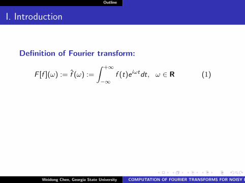
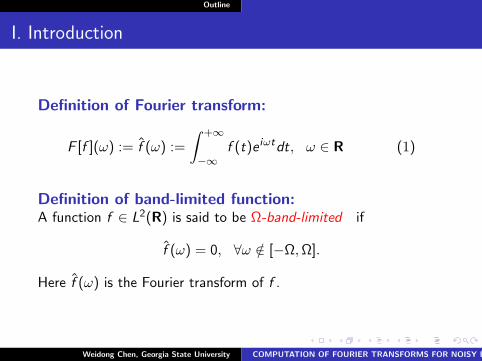
Definition of Fourier transform:
F [f ](ω) := f (ω) :=
∫ +∞
−∞f (t)e iωtdt, ω ∈ R (1)
Definition of band-limited function:A function f ∈ L2(R) is said to be Ω-band-limited if
f (ω) = 0, ∀ω /∈ [−Ω,Ω].
Here f (ω) is the Fourier transform of f .
Weidong Chen, Georgia State University COMPUTATION OF FOURIER TRANSFORMS FOR NOISY BANDLIMITED SIGNALS
Outline
I. Introduction
Definition of Fourier transform:
F [f ](ω) := f (ω) :=
∫ +∞
−∞f (t)e iωtdt, ω ∈ R (1)
Definition of band-limited function:A function f ∈ L2(R) is said to be Ω-band-limited if
f (ω) = 0, ∀ω /∈ [−Ω,Ω].
Here f (ω) is the Fourier transform of f .
Weidong Chen, Georgia State University COMPUTATION OF FOURIER TRANSFORMS FOR NOISY BANDLIMITED SIGNALS
Outline
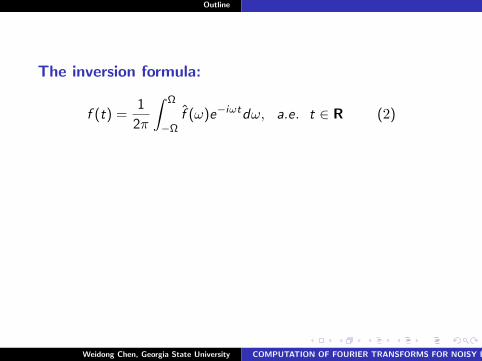
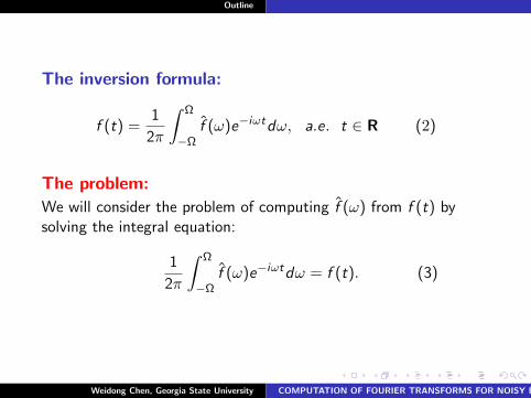
The inversion formula:
f (t) =1
2π
∫ Ω
−Ωf (ω)e−iωtdω, a.e. t ∈ R (2)
The problem:
We will consider the problem of computing f (ω) from f (t) bysolving the integral equation:
1
2π
∫ Ω
−Ωf (ω)e−iωtdω = f (t). (3)
Weidong Chen, Georgia State University COMPUTATION OF FOURIER TRANSFORMS FOR NOISY BANDLIMITED SIGNALS
Outline
Sampling Theorem
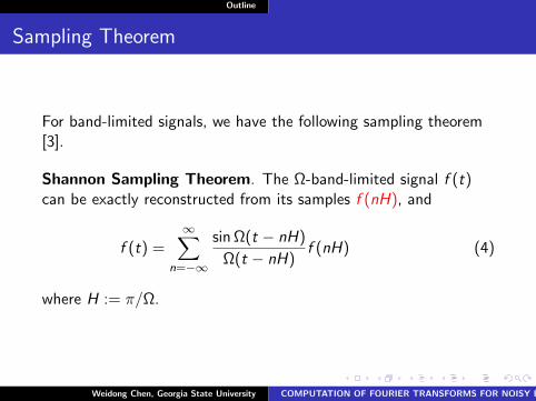
For band-limited signals, we have the following sampling theorem[3].
Shannon Sampling Theorem. The Ω-band-limited signal f (t)can be exactly reconstructed from its samples f (nH), and
f (t) =∞∑
n=−∞
sin Ω(t − nH)
Ω(t − nH)f (nH) (4)
where H := π/Ω.
Weidong Chen, Georgia State University COMPUTATION OF FOURIER TRANSFORMS FOR NOISY BANDLIMITED SIGNALS

Outline
Fourier Serious
Calculating the Fourier transform of f (t) by the formula (4), wehave the formula which is same as the Fourier series [4] p.3
f (ω) = H∞∑
n=−∞f (nH)e inHωP[−Ω, Ω] (5)
where P[−Ω,Ω] is the characteristic function of [−Ω,Ω].
Weidong Chen, Georgia State University COMPUTATION OF FOURIER TRANSFORMS FOR NOISY BANDLIMITED SIGNALS
Outline
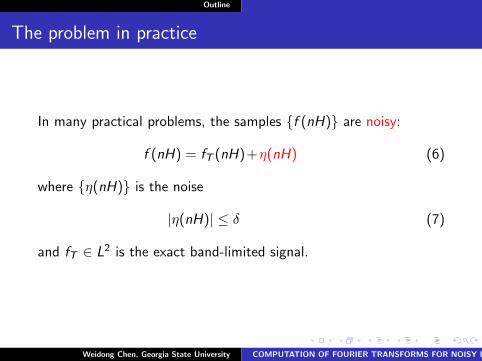
The problem in practice
In many practical problems, the samples f (nH) are noisy:
f (nH) = fT (nH)+η(nH) (6)
where η(nH) is the noise
|η(nH)| ≤ δ (7)
and fT ∈ L2 is the exact band-limited signal.
Weidong Chen, Georgia State University COMPUTATION OF FOURIER TRANSFORMS FOR NOISY BANDLIMITED SIGNALS
Outline
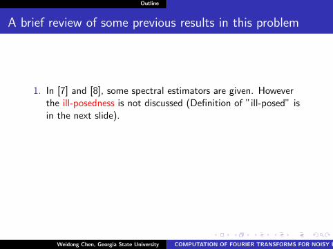
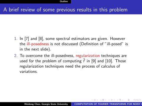
A brief review of some previous results in this problem
1. In [7] and [8], some spectral estimators are given. Howeverthe ill-posedness is not discussed (Definition of ”ill-posed” isin the next slide).
2. To overcome the ill-posedness, regularization techniques areused for the problem of computing f in [9] and [10]. Thoseregularization techniques need the process of calculus ofvariations.
Weidong Chen, Georgia State University COMPUTATION OF FOURIER TRANSFORMS FOR NOISY BANDLIMITED SIGNALS
Outline
II. The Ill-posedness of the Problem
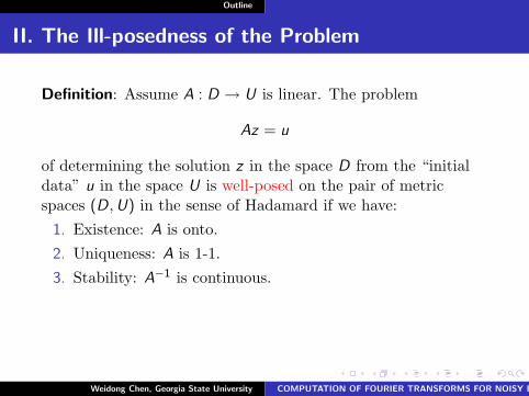
Definition: Assume A : D → U is linear. The problem
Az = u
of determining the solution z in the space D from the “initialdata” u in the space U is well-posed on the pair of metricspaces (D,U) in the sense of Hadamard if we have:
1. Existence: A is onto.2. Uniqueness: A is 1-1.3. Stability: A−1 is continuous.
Remark:Problems that violate any of the three conditions are ill-posed.
Weidong Chen, Georgia State University COMPUTATION OF FOURIER TRANSFORMS FOR NOISY BANDLIMITED SIGNALS
Outline
II. The Ill-posedness of the Problem
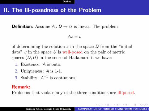
Definition: Assume A : D → U is linear. The problem
Az = u
of determining the solution z in the space D from the “initialdata” u in the space U is well-posed on the pair of metricspaces (D,U) in the sense of Hadamard if we have:
1. Existence: A is onto.2. Uniqueness: A is 1-1.3. Stability: A−1 is continuous.
Remark:Problems that violate any of the three conditions are ill-posed.
Weidong Chen, Georgia State University COMPUTATION OF FOURIER TRANSFORMS FOR NOISY BANDLIMITED SIGNALS
Outline
The Definition of the Operator A
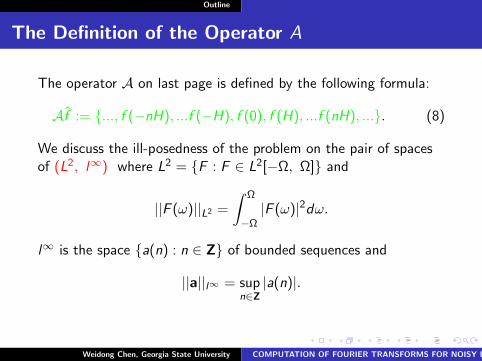
The operator A on last page is defined by the following formula:
Af := ..., f (−nH), ...f (−H), f (0), f (H), ...f (nH), .... (8)
We discuss the ill-posedness of the problem on the pair of spacesof (L2, l∞) where L2 = F : F ∈ L2[−Ω, Ω] and
||F (ω)||L2 =
∫ Ω
−Ω|F (ω)|2dω.
l∞ is the space a(n) : n ∈ Z of bounded sequences and
||a||l∞ = supn∈Z
|a(n)|.
Weidong Chen, Georgia State University COMPUTATION OF FOURIER TRANSFORMS FOR NOISY BANDLIMITED SIGNALS
Outline
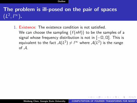
The problem is ill-posed on the pair of spaces(L2, l∞).
1. Existence: The existence condition is not satisfied.We can choose the sampling f (nH) to be the samples of asignal whose frequency distribution is not in [−Ω,Ω]. This isequivalent to the fact A(L2) 6= l∞ where A(L2) is the rangeof A.
2. Uniqueness: The uniqueness condition is satisfied, sincef (nH) ≡ 0 implies f (t) ≡ 0. So A is injective.
3. Stability: The stability condition is not satisfied. In otherwords, A−1 is not continuous from A(L2) to L2.
Proof of Instability
By Parseval equality, ||η||2 = 2πH∑∞
n=−∞ |η(nH)|2, it is easy tosee the stability condition is not satisfied. So, this is a highlyill-posed problem.
Weidong Chen, Georgia State University COMPUTATION OF FOURIER TRANSFORMS FOR NOISY BANDLIMITED SIGNALS
Outline
III. Regularization method
Definition of regularizing operator:
AssumeAze = ue (”e” for exact).
An operator R(∗, α) : U → D, depending on a parameter α, iscalled a regularizing operator for the equation Az = u in aneighborhood of ue if there exists a function α = α(δ) of δ suchthat if
limδ→0
||uδ − ue || = 0 and zα = R(uδ, α(δ))
thenlimδ→0
||zα − ze || = 0.
The approximate solution zα = R(u, α) to the exact solution ze
obtained by the method of regularization is called a regularizedsolution.
Weidong Chen, Georgia State University COMPUTATION OF FOURIER TRANSFORMS FOR NOISY BANDLIMITED SIGNALS
Outline
Regularized Fourier Transform
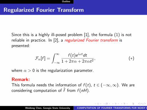
Since this is a highly ill-posed problem [1], the formula (1) is notreliable in practice. In [2], a regularized Fourier transform ispresented:
Fα[f ] =
∫ ∞
−∞
f (t)e iωtdt
1 + 2πα + 2παt2, (∗)
where α > 0 is the regularization parameter.
Remark:This formula needs the information of f (t), t ∈ (−∞,∞). We areconsidering computation of f from f (nH).
Weidong Chen, Georgia State University COMPUTATION OF FOURIER TRANSFORMS FOR NOISY BANDLIMITED SIGNALS
Outline
Regularized Fourier Transform
Since this is a highly ill-posed problem [1], the formula (1) is notreliable in practice. In [2], a regularized Fourier transform ispresented:
Fα[f ] =
∫ ∞
−∞
f (t)e iωtdt
1 + 2πα + 2παt2, (∗)
where α > 0 is the regularization parameter.
Remark:This formula needs the information of f (t), t ∈ (−∞,∞). We areconsidering computation of f from f (nH).
Weidong Chen, Georgia State University COMPUTATION OF FOURIER TRANSFORMS FOR NOISY BANDLIMITED SIGNALS
Outline
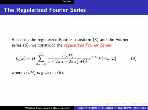
The Regularized Fourier Series
Based on the regularized Fourier transform (3) and the Fourierseries (5), we construct the regularized Fourier Series:
fα(ω) = H∞∑
n=−∞
f (nH)
1 + 2πα + 2πα(nH)2e inHωP[−Ω,Ω] (9)
where f (nH) is given in (6).
Weidong Chen, Georgia State University COMPUTATION OF FOURIER TRANSFORMS FOR NOISY BANDLIMITED SIGNALS
Outline
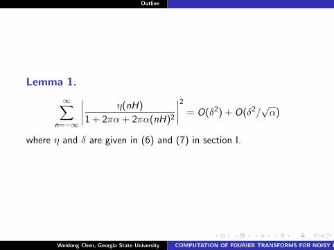
Lemma 1.
∞∑n=−∞
∣∣∣∣ η(nH)
1 + 2πα + 2πα(nH)2
∣∣∣∣2 = O(δ2) + O(δ2/√
α)
where η and δ are given in (6) and (7) in section I.
Weidong Chen, Georgia State University COMPUTATION OF FOURIER TRANSFORMS FOR NOISY BANDLIMITED SIGNALS
Outline
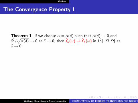
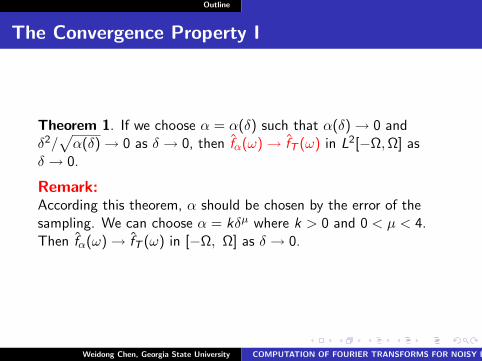
The Convergence Property I
Theorem 1. If we choose α = α(δ) such that α(δ) → 0 andδ2/
√α(δ) → 0 as δ → 0, then fα(ω) → fT (ω) in L2[−Ω,Ω] as
δ → 0.
Remark:According this theorem, α should be chosen by the error of thesampling. We can choose α = kδµ where k > 0 and 0 < µ < 4.Then fα(ω) → fT (ω) in [−Ω, Ω] as δ → 0.
Weidong Chen, Georgia State University COMPUTATION OF FOURIER TRANSFORMS FOR NOISY BANDLIMITED SIGNALS
Outline
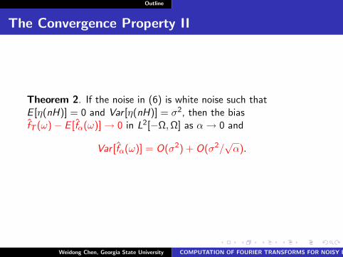
The Convergence Property II
Theorem 2. If the noise in (6) is white noise such thatE [η(nH)] = 0 and Var [η(nH)] = σ2, then the biasfT (ω)− E [fα(ω)] → 0 in L2[−Ω,Ω] as α → 0 and
Var [fα(ω)] = O(σ2) + O(σ2/√
α).
Weidong Chen, Georgia State University COMPUTATION OF FOURIER TRANSFORMS FOR NOISY BANDLIMITED SIGNALS
Outline
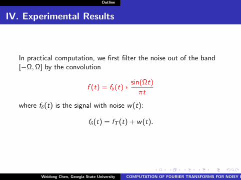
IV. Experimental Results
In practical computation, we first filter the noise out of the band[−Ω,Ω] by the convolution
f (t) = fδ(t) ∗sin(Ωt)
πt
where fδ(t) is the signal with noise w(t):
fδ(t) = fT (t) + w(t).
Weidong Chen, Georgia State University COMPUTATION OF FOURIER TRANSFORMS FOR NOISY BANDLIMITED SIGNALS
Outline
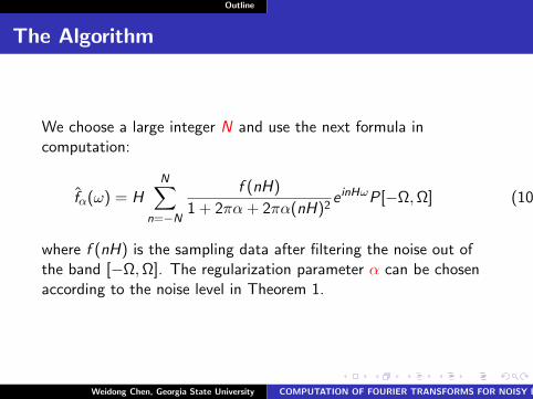
The Algorithm
We choose a large integer N and use the next formula incomputation:
fα(ω) = HN∑
n=−N
f (nH)
1 + 2πα + 2πα(nH)2e inHωP[−Ω,Ω] (10)
where f (nH) is the sampling data after filtering the noise out ofthe band [−Ω,Ω]. The regularization parameter α can be chosenaccording to the noise level in Theorem 1.
Weidong Chen, Georgia State University COMPUTATION OF FOURIER TRANSFORMS FOR NOISY BANDLIMITED SIGNALS
Outline
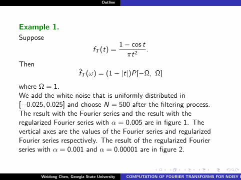
Example 1.
Suppose
fT (t) =1− cos t
πt2.
ThenfT (ω) = (1− |t|)P[−Ω, Ω]
where Ω = 1.We add the white noise that is uniformly distributed in[−0.025, 0.025] and choose N = 500 after the filtering process.The result with the Fourier series and the result with theregularized Fourier series with α = 0.005 are in figure 1. Thevertical axes are the values of the Fourier series and regularizedFourier series respectively. The result of the regularized Fourierseries with α = 0.001 and α = 0.00001 are in figure 2.
Weidong Chen, Georgia State University COMPUTATION OF FOURIER TRANSFORMS FOR NOISY BANDLIMITED SIGNALS
Outline
Discussion on the result
From the numerical results in Figure 1 and Figure 2, we can seethat bias is smaller if α is reduced from 0.005 to 0.001. Thismeans that fT (ω)− E [f (ω)] is close to zero which is the result ofTheorem 2. However if α is too small such as the caseα = 0.000001 in Figure 2, the error of the regularized Fourierseries is large. This is due to the second term O(σ/
√α) in the
estimation of Var [f (ω)] in Theorem 2.
Weidong Chen, Georgia State University COMPUTATION OF FOURIER TRANSFORMS FOR NOISY BANDLIMITED SIGNALS
Outline
The Tikhonov regularization method I
In example 2, we will compare the regularized Fourier series withthe Tikhonov regularization method used in [1], [9] and [10]. Weintroduce the Tikhonov regularization method next.First we write equation (2) by the finite difference method
Af = f
where
A =
(1
2πe iωj tk h
)(2N+1)×(2M+1)
, h = Ω/M
andf = (f−M , ..., f0, ..., fM)
f = (f−N , ..., f0, ..., fN).
Weidong Chen, Georgia State University COMPUTATION OF FOURIER TRANSFORMS FOR NOISY BANDLIMITED SIGNALS
Outline
The Tikhonov regularization method II
Define the smoothing functional
Mα[f , f ] = ||Af − f ||2 + α||f ||2.
Here the norms of f and f are defined by
||f ||2 =M∑
j=−M
|fj |2, ||f ||2 =N∑
k=−N
|fk |2.
We can find the approximate Fourier transform by minimizingMα[f , f ]. And the minimizer is the solution of the Euler equation(
ATA + αI)
f = AT f .
Weidong Chen, Georgia State University COMPUTATION OF FOURIER TRANSFORMS FOR NOISY BANDLIMITED SIGNALS
Outline
Example 2.
The signals are the same as the signals in Example 1. We chooseM=400. The results of the regularized Fourier series and theTikhonov regularized solution with α = 0.001 are in Figure 3, 4and 5 for the cases H = π, H = π/10 and H = π/50.We can see that if H is smaller the Tikhonov regularized solution ismore accurate, but it is not as good as the regularized Fourierseries.
Weidong Chen, Georgia State University COMPUTATION OF FOURIER TRANSFORMS FOR NOISY BANDLIMITED SIGNALS
Outline
References I
A. N. Tikhonov and V. Y. Arsenin,Solution of Ill-Posed Problems.Winston/Wiley, 1977.
W. Chen,An Efficient Method for An Ill-posed Problem—Band-limitedExtrapolation by Regularization.IEEE Trans. on Signal Processing, vol 54, pp.4611-4618, 2006.
C. E. Shannon,A mathematical theory of communication.The Bell System Technical Journal, vol. 27, July 1948.
J. R. Higgins,Sampling Theory in Fourier and Signal Analysis Foundations.Oxford University Press Inc., New York, 1996.
Weidong Chen, Georgia State University COMPUTATION OF FOURIER TRANSFORMS FOR NOISY BANDLIMITED SIGNALS
Outline
References II
R. Bhatia,Fourier Series.The Mathematical Association of American, 2005.
A. Steiner,Plancherel’s Theorem and the Shannon Series DerivedSimultaneously.The American Mathematical Monthly, vol. 87, no. 3, Mar.1980, pp. 193-197.
A. R. Nematollahi,Spectral Estimation of Stationary Time Series: RecentDevelopments.J. Statist. Res. Iran 2, 2005, pp.107-127..
Weidong Chen, Georgia State University COMPUTATION OF FOURIER TRANSFORMS FOR NOISY BANDLIMITED SIGNALS
Outline
References III
S. V. Narasimhan and M. Harish,Spectral estimation based on discrete cosine transform andmodified group delay.Signal Processing 86, 2004, pp.279-305..
H. Kim, B. Yang and B. Lee,Iterative Fourier transform algorithm with regularization forthe optimal design of diffractive optical elements.J. Opt. Soc. Am. A Vol. 21, No. 12, pp. 2353-2356, 2004.
I. V. Lyuboshenko and A. M. Akhmetshin,Regularization Of The Problem Of Image Restoration From ItsNoisy Fourier Transform Phase.International Conference on Image Processing, Volume 1, 1996pp. 793 - 796.
Weidong Chen, Georgia State University COMPUTATION OF FOURIER TRANSFORMS FOR NOISY BANDLIMITED SIGNALS

![[Eleutheria, iwanna, georgia]](https://static.fdocument.org/doc/165x107/55ccd4b6bb61eb3f6f8b4843/eleutheria-iwanna-georgia.jpg)