Chapter 3 Fourier Transforms of...

Chapter 3

Fourier Transforms of

Distributions

Questions

1) How do we transform a function f /∈ L1(R), f /∈ L2(R), for example

Weierstrass function

σ(t) =

∞∑

k=0

ak cos(2πbkt),

where b 6= integer (if b is an integer, then σ is periodic and we can use

Chapter I)?

2) Can we interpret both the periodic F -transform (on L1(T)) and the Fourier

integral (on L1(R)) as special cases of a “more general” Fourier transform?

3) How do you differentiate a discontinuous function?

The answer: Use “distribution theory”, developed in France by Schwartz in

1950’s.

3.1 What is a Measure?

We start with a simpler question: what is a “δ-function”? Typical definition:

δ(x) = 0, x 6= 0

δ(0) = ∞∫ ε−εδ(x)dx = 1, (for ε > 0).

67

CHAPTER 3. FOURIER TRANSFORMS OF DISTRIBUTIONS 68

We observe: This is pure nonsense. We observe that δ(x) = 0 a.e., so∫ ε−εδ(x)dx = 0.

Thus: The δ-function is not a function! What is it?

Normally a δ-function is used in the following way: Suppose that f is continuous

at the origin. Then

∫ ∞

−∞

f(x)δ(x)dx =

∫ ∞

−∞

[f(x) − f(0)]︸︷︷︸=0

when x=0

δ(x)︸︷︷︸=0

when x 6=0

dx+ f(0)

∫ ∞

−∞

δ(x)dx

= f(0)

∫ ∞

−∞

δ(x)dx = f(0).

This gives us a new interpretation of δ:

The δ-function is the “operator” which evaluates a continuous function at the

point zero.

Principle: You feed a function f(x) to δ, and δ gives you back the number

f(0) (forget about the integral formula).

Since the formal integral∫∞

−∞f(x)δ(x)dx resembles an inner product, we often

use the notation 〈δ, f〉. Thus

〈δ, f〉 = f(0)

Definition 3.1. The δ-operator is the (bounded linear) operator which maps

f ∈ C0(R) into the number f(0). Also called Dirac’s delta .

This is a special case of measure:

Definition 3.2. A measure µ is a bounded linear operator which maps func-

tions f ∈ C0(R) into the set of complex numbers C (or real). We denote this

number by 〈µ, f〉.

Example 3.3. The operator which maps f ∈ C0(R) into the number

f(0) + f(1) +

∫ 1

0

f(s)ds

is a measure.

Proof. Denote 〈G, f〉 = f(0) + f(1) +∫ 1

0f(s)ds. Then


i) G maps C0(R) → C.

ii) G is linear :

〈G, λf + µg〉 = λf(0) + µg(0) + λf(1) + µg(1)

+

∫ 1

0

(λf(s) + µg(s))ds

= λf(0) + λf(1) +

∫ 1

0

λf(s)ds

+µg(0) + µg(1) +

∫ 1

0

µg(s)ds

= λ〈G, f〉 + µ〈G, g〉.

iii) G is continuous : If fn → f in C0(R), then maxt∈R|fn(t) − f(t)| → 0 as

n→ ∞, so

fn(0) → f(0), fn(1) → f(1) and

∫ 1

0

fn(s)ds→

∫ 1

0

f(s)ds,

so

〈G, fn〉 → 〈G, f〉 as n→ ∞.

Thus, G is a measure.

Warning 3.4. 〈G, f〉 is linear in f , not conjugate linear:

〈G, λf〉 = λ〈G, f〉, and not = λ〈G, f〉.

Alternative notation 3.5. Instead of 〈G, f〉 many people write G(f) or Gf

(for example , Gripenberg). See Gasquet for more details.

3.2 What is a Distribution?

Physisists often also use “the derivative of a δ-function”, which is defined as

〈δ′, f〉 = −f ′(0),

here f ′(0) = derivative of f at zero. This is not a measure: It is not defined

for all f ∈ C0(R) (only for those that are differentiable at zero). It is linear,

but it is not continuous (easy to prove). This is an example of a more general

distribution.


Definition 3.6. A tempered distribution (=tempererad distribution) is a

continuous linear operator from S to C. We denote the set of such distributions

by S ′. (The set S was defined in Section 2.2).

Theorem 3.7. Every measure is a distribution.

Proof.

i) Maps S into C, since S ⊂ C0(R).

ii) Linearity is OK.

iii) Continuity is OK: If fn → f in S, then fn → f in C0(R), so 〈µ, fn〉 → 〈µ, f〉

(more details below!)

Example 3.8. Define 〈δ′, ϕ〉 = −ϕ′(0), ϕ ∈ S. Then δ′ is a tempered distribu-

tion

Proof.

i) Maps S → C? Yes!

ii) Linear? Yes!

iii) Continuous? Yes!

(See below for details!)

What does ϕn → ϕ in S mean?

Definition 3.9. ϕn → ϕ in S means the following: For all positive integers k, m,

tkϕ(m)n (t) → tkϕ(m)(t)

uniformly in t, i.e.,

limn→∞

maxt∈R

|tk(ϕ(m)n (t) − ϕ(m)(t))| = 0.

Lemma 3.10. If ϕn → ϕ in S, then

ϕ(m)n → ϕ(m) in C0(R)

for all m = 0, 1, 2, . . .

Proof. Obvious.

Proof that δ′ is continuous: If ϕn → ϕ in S, then maxt∈R|ϕ′n(t) − ϕ′(t)| → 0

as n→ ∞, so

〈δ′, ϕn〉 = −ϕ′n(0) → ϕ′(0) = 〈δ′, ϕ〉.


3.3 How to Interpret a Function as a Distribu-

tion?

Lemma 3.11. If f ∈ L1(R) then the operator which maps ϕ ∈ S into

〈F, ϕ〉 =

∫ ∞

−∞

f(s)ϕ(s)ds

is a continuous linear map from S to C. (Thus, F is a tempered distribution).

Note: No complex conjugate on ϕ!

Note: F is even a measure.

Proof.

i) For every ϕ ∈ S, the integral converges (absolutely), and defines a number

in C. Thus, F maps S → C.

ii) Linearity : for all ϕ, ψ ∈ S and λ, µ ∈ C,

〈F, λϕ+ µψ〉 =

∫

R

f(s)[λϕ(s) + µψ(s)]ds

= λ

∫

R

f(s)ϕ(s)ds+ µ

∫

R

f(s)ψ(s)ds

= λ〈F, ϕ〉 + µ〈F, ψ〉.

iii) Continuity : If ϕn → ϕ in S, then ϕn → ϕ in C0(R), and by Lebesgue’s

dominated convergence theorem,

〈F, ϕn〉 =

∫

R

f(s)ϕn(s)ds→

∫

R

f(s)ϕ(s)ds = 〈F, ϕ〉.

The same proof plus a little additional work proves:

Theorem 3.12. If ∫ ∞

−∞

|f(t)|

1 + |t|ndt <∞

for some n = 0, 1, 2, . . ., then the formula

〈F, ϕ〉 =

∫ ∞

−∞

f(s)ϕ(s)ds, ϕ ∈ S,

defines a tempered distribution F .


Definition 3.13. We call the distribution F in Lemma 3.11 and Theorem 3.12

the distribution induced by f , and often write 〈f, ϕ〉 instead of 〈F, ϕ〉. Thus,

〈f, ϕ〉 =

∫ ∞

−∞

f(s)ϕ(s)ds, ϕ ∈ S.

This is sort of like an inner product, but we cannot change places of f and ϕ: f

is “the distribution” and ϕ is “the test function” in 〈f, ϕ〉.

Does “the distribution f” determine “the function f” uniquely? Yes!

Theorem 3.14. Suppose that the two functions f1 and f2 satisfy∫

R

|fi(t)|

1 + |t|ndt <∞ (i = 1 or i = 2),

and that they induce the same distribution, i.e., that∫

R

f1(t)ϕ(t)dt =

∫

R

f2(t)ϕ(t)dt, ϕ ∈ S.

Then f1(t) = f2(t) almost everywhere.

Proof. Let g = f1 − f2. Then

∫

R

g(t)ϕ(t)dt = 0 for all ϕ ∈ S ⇐⇒

∫

R

g(t)

(1 + t2)n/2(1 + t2)n/2ϕ(t)dt = 0 ∀ϕ ∈ S.

Easy to show that (1 + t2)n/2ϕ(t)︸︷︷︸ψ(t)

∈ S ⇐⇒ ϕ ∈ S. If we define h(t) = g(t)

(1+t2)n/2 ,

then h ∈ L1(R), and∫ ∞

−∞

h(s)ψ(s)ds = 0 ∀ψ ∈ S.

If ψ ∈ S then also the function s 7→ ψ(t− s) belongs to S, so

∫

R

h(s)ψ(t− s)ds = 0

∀ψ ∈ S,

∀t ∈ R.(3.1)

Take ψn(s) = ne−π(ns)2 . Then ψn ∈ S, and by 3.1,

ψn ∗ h ≡ 0.

On the other hand, by Theorem 2.12, ψn ∗ h → h in L1(R) as n → ∞, so this

gives h(t) = 0 a.e.


Corollary 3.15. If we know “the distribution f”, then from this knowledge we

can reconstruct f(t) for almost all t.

Proof. Use the same method as above. We know that h(t) ∈ L1(R), and that

(ψn ∗ h)(t) → h(t) =f(t)

(1 + t2)n/2.

As soon as we know “the distribution f”, we also know the values of

(ψn ∗ h)(t) =

∫ ∞

−∞

f(s)

(1 + s2)n/2(1 + s2)n/2ψn(t− s)ds

for all t.

3.4 Calculus with Distributions

(=Rakneregler)

3.16 (Addition). If f and g are two distributions, then f + g is the distribution

〈f + g, ϕ〉 = 〈f, ϕ〉 + 〈g, ϕ〉, ϕ ∈ S.

(f and g distributions ⇐⇒ f ∈ S ′ and g ∈ S ′).

3.17 (Multiplication by a constant). If λ is a constant and f ∈ S ′, then λf is

the distribution

〈λf, ϕ〉 = λ〈f, ϕ〉, ϕ ∈ S.

3.18 (Multiplication by a test function). If f ∈ S ′ and η ∈ S, then ηf is the

distribution

〈ηf, ϕ〉 = 〈f, ηϕ〉 ϕ ∈ S.

Motivation: If f would be induced by a function, then this would be the natural

definition, because∫

R

[η(s)f(s)]ϕ(s)ds =

∫

R

f(s)[η(s)ϕ(s)]ds = 〈f, ηϕ〉.

Warning 3.19. In general, you cannot multiply two distributions. For example,

δ2 = δδ is nonsense(δ = “δ-function”)

=Dirac’s delta


However, it is possible to multiply distributions by a larger class of “test func-

tions”:

Definition 3.20. By the class C∞pol(R) of tempered test functions we mean the

following:

ψ ∈ C∞pol(R) ⇐⇒ f ∈ C∞(R),

and for every k = 0, 1, 2, . . . there are two numbers M and n so that

|ψ(k)(t)| ≤M(1 + |t|n), t ∈ R.

Thus, f ∈ C∞pol(R) ⇐⇒ f ∈ C∞(R), and every derivative of f grows at most as

a polynomial as t→ ∞.

Repetition:

S = “rapidly decaying test functions”

S ′ = “tempered distributions”

C∞pol(R) = “tempered test functions”.

Example 3.21. Every polynomial belongs to C∞pol. So do the functions

1

1 + x2, (1 + x2)±m (m need not be an integer)

Lemma 3.22. If ψ ∈ C∞pol(R) and ϕ ∈ S, then

ψϕ ∈ S.

Proof. Easy (special case used on page 72).

Definition 3.23. If ψ ∈ C∞pol(R) and f ∈ S ′, then ψf is the distribution

〈ψf, ϕ〉 = 〈f, ψϕ〉, ϕ ∈ S

(O.K. since ψϕ ∈ S).

Now to the big surprise : Every distribution has a derivative, which is another

distribution!

Definition 3.24. Let f ∈ S ′. Then the distribution derivative of f is the

distribution defined by

〈f ′, ϕ〉 = −〈f, ϕ′〉, ϕ ∈ S

(This is O.K., because ϕ ∈ S =⇒ ϕ′ ∈ S, so −〈f, ϕ′〉 is defined).


Motivation: If f would be a function in C1(R) (not too big at ∞), then

〈f, ϕ′〉 =

∫ ∞

−∞

f(s)ϕ′(s)ds (integrate by parts)

= [f(s)ϕ(s)]∞−∞︸︷︷︸=0

−

∫ ∞

−∞

f ′(s)ϕ(s)ds

= −〈f ′, ϕ〉.

Example 3.25. Let

f(t) =

e−t, t ≥ 0,

−et, t < 0.

Interpret this as a distribution, and compute its distribution derivative.

Solution:

〈f ′, ϕ〉 = −〈f, ϕ′〉 = −

∫ ∞

−∞

f(s)ϕ′(s)ds

=

∫ 0

−∞

esϕ′(s)ds−

∫ ∞

0

e−sϕ′(s)ds

= [esϕ(s)]0−∞ −

∫ 0

−∞

esϕ(s)ds−[e−sϕ(s)

]∞0−

∫ ∞

0

e−sϕ(s)ds

= 2ϕ(0) −

∫ ∞

−∞

e−|s|ϕ(s)ds.

Thus, f ′ = 2δ + h, where h is the “function” h(s) = −e−|s|, s ∈ R, and δ = the

Dirac delta (note that h ∈ L1(R) ∩ C(R)).

Example 3.26. Compute the second derivative of the function in Example 3.25!

Solution: By definition, 〈f ′′, ϕ〉 = −〈f ′, ϕ′〉. Put ϕ′ = ψ, and apply the rule

〈f ′, ψ〉 = −〈f, ψ′〉. This gives

〈f ′′, ϕ〉 = 〈f, ϕ′′〉.

By the preceding computation

−〈f, ϕ′〉 = −2ϕ′(0) −

∫ ∞

−∞

e−|s|ϕ′(s)ds

= (after an integration by parts)

= −2ϕ′(0) +

∫ ∞

−∞

f(s)ϕ(s)ds


(f = original function). Thus,

〈f ′′, ϕ〉 = −2ϕ′(0) +

∫ ∞

−∞

f(s)ϕ(s)ds.

Conclusion: In the distribution sense,

f ′′ = 2δ′ + f,

where 〈δ′, ϕ〉 = −ϕ′(0). This is the distribution derivative of Dirac’s delta. In

particular: f is a distribution solution of the differential equation

f ′′ − f = 2δ′.

This has something to do with the differential equation on page 59. More about

this later.

3.5 The Fourier Transform of a Distribution

Repetition: By Lemma 2.19, we have

∫ ∞

−∞

f(t)g(t)dt =

∫ ∞

−∞

f(t)g(t)dt

if f, g ∈ L1(R). Take g = ϕ ∈ S. Then ϕ ∈ S (See Theorem 2.24), so we can

interpret both f and f in the distribution sense and get

Definition 3.27. The Fourier transform of a distribution f ∈ S is the distribu-

tion defined by

〈f , ϕ〉 = 〈f, ϕ〉, ϕ ∈ S.

Possible, since ϕ ∈ S ⇐⇒ ϕ ∈ S.

Problem: Is this really a distribution? It is well-defined and linear, but is it

continuous? To prove this we need to know that

ϕn → ϕ in S ⇐⇒ ϕn → ϕ in S.

This is a true statement (see Gripenberg or Gasquet for a proof), and we get

Theorem 3.28. The Fourier transform maps the class of tempered distributions

onto itself:

f ∈ S ′ ⇐⇒ f ∈ S ′.


There is an obvious way of computing the inverse Fourier transform:

Theorem 3.29. The inverse Fourier transform f of a distribution f ∈ S ′ is

given by

〈f, ϕ〉 = 〈f , ψ〉, ϕ ∈ S,

where ψ = the inverse Fourier transform of ϕ, i.e., ψ(t) =∫∞

−∞e2πitωϕ(ω)dω.

Proof. If ψ = the inverse Fourier transform of ϕ, then ϕ = ψ and the formula

simply says that 〈f, ψ〉 = 〈f , ψ〉.

3.6 The Fourier Transform of a Derivative

Problem 3.30. Let f ∈ S ′. Then f ′ ∈ S ′. Find the Fourier transform of f ′.

Solution: Define η(t) = 2πit, t ∈ R. Then η ∈ C∞pol, so we can multiply a

tempered distribution by η. By various definitions (start with 3.27)

〈(f ′), ϕ〉 = 〈f ′, ϕ〉 (use Definition 3.24)

= −〈f, (ϕ)′〉 (use Theorem 2.7(g))

= −〈f, ψ〉 (where ψ(s) = −2πisϕ(s))

= −〈f , ψ〉 (by Definition 3.27)

= 〈f , ηϕ〉 (see Definition above of η)

= 〈ηf , ϕ〉 (by Definition 3.23).

Thus, (f ′) = ηf where η(ω) = 2πiω, ω ∈ R.

This proves one half of:

Theorem 3.31.

(f ′) = (i2πω)f and

(−2πitf) = (f)′

More precisely, if we define η(t) = 2πit, then η ∈ C∞pol, and

(f ′) = ηf , (ηf) = −f ′.

By repeating this result several times we get

Theorem 3.32.

(f (k)) = (2πiω)kf k ∈ Z+

( (−2πit)kf) = f (k).


Example 3.33. Compute the Fourier transform of

f(t) =

e−t, t > 0,

−et, t < 0.

Smart solution: By the Examples 3.25 and 3.26.

f ′′ = 2δ′ + f (in the distribution sense).

Transform this:

[(2πiω)2 − 1]f = 2(δ′) = 2(2πiω)δ

(since δ′ is the derivative of δ). Thus, we need δ:

〈δ, ϕ〉 = 〈δ, ϕ〉 = ϕ(0) =

∫

R

ϕ(s)ds

=

∫

R

1 · ϕ(s)ds =

∫

R

f(s)ϕ(s)ds,

where f(s) ≡ 1. Thus δ is the distribution which is induced by the function

f(s) ≡ 1, i.e., we may write δ ≡ 1 .

Thus, −(4π2ω2 + 1)f = 4πiω, so f is induced by the function 4πiω−(1+4π2ω2)

. Thus,

f(ω) =4πiω

−(1 + 4π2ω2).

In particular:

Lemma 3.34.

δ(ω) ≡ 1 and

1 = δ.

(The Fourier transform of δ is the function ≡ 1, and the Fourier transform of

the function ≡ 1 is the Dirac delta.)

Combining this with Theorem 3.32 we get

Lemma 3.35.

δ(k) = (2πiω)k, k ∈ Z+ = 0, 1, 2, . . .[(−2πit)k

]= δ(k)


3.7 Convolutions (”Faltningar”)

It is sometimes (but not always) possible to define the convolution of two distri-

butions. One possibility is the following: If ϕ, ψ ∈ S, then we know that

(ϕ ∗ ψ) = ϕψ,

so we can define ϕ ∗ψ to be the inverse Fourier transform of ϕψ. The same idea

applies to distributions in some cases:

Definition 3.36. Let f ∈ S ′ and suppose that g ∈ S ′ happens to be such that

g ∈ C∞pol(R) (i.e., g is induced by a function in C∞

pol(R), i.e., g is the inverse

F -transform of a function in C∞pol). Then we define

f ∗ g = the inverse Fourier transform of f g,

i.e. (cf. page 77):

〈f ∗ g, ϕ〉 = 〈f g, ϕ〉

where ϕ is the inverse Fourier transform of ϕ:

ϕ(t) =

∫ ∞

−∞

e2πiωtϕ(ω)dω.

This is possible since g ∈ C∞pol, so that f g ∈ S ′; see page 74

To get a direct interpretation (which does not involve Fourier transforms) we

need two more definitions:

Definition 3.37. Let t ∈ R, f ∈ S ′, ϕ ∈ S. Then the translations τtfand τtϕ

are given by

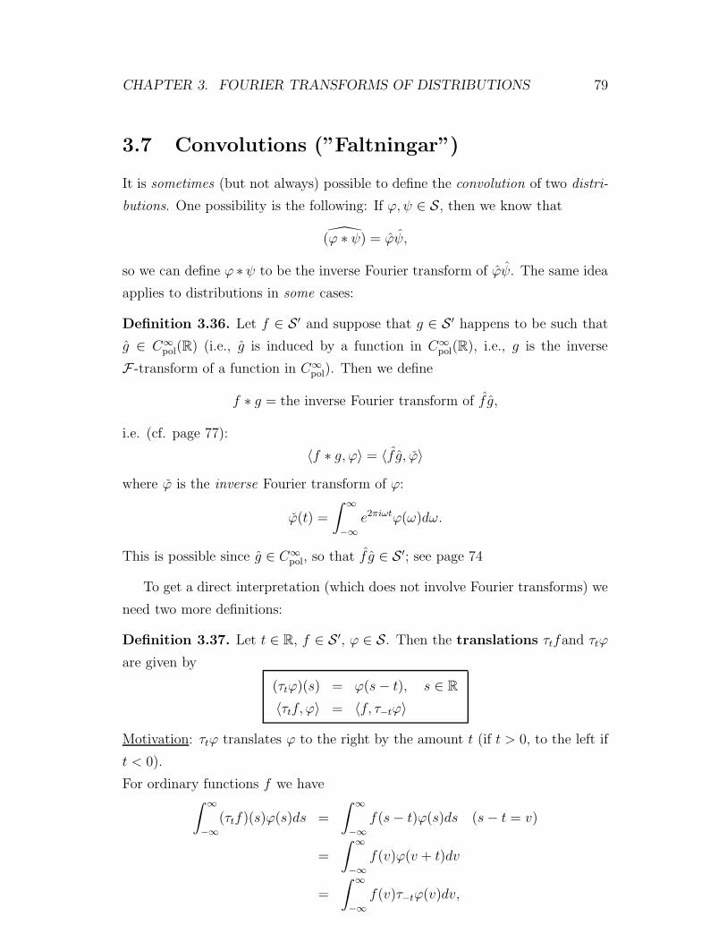
(τtϕ)(s) = ϕ(s− t), s ∈ R

〈τtf, ϕ〉 = 〈f, τ−tϕ〉

Motivation: τtϕ translates ϕ to the right by the amount t (if t > 0, to the left if

t < 0).

For ordinary functions f we have∫ ∞

−∞

(τtf)(s)ϕ(s)ds =

∫ ∞

−∞

f(s− t)ϕ(s)ds (s− t = v)

=

∫ ∞

−∞

f(v)ϕ(v + t)dv

=

∫ ∞

−∞

f(v)τ−tϕ(v)dv,


t

τ ϕt

ϕ

so the distribution definition coincides with the usual definition for functions

interpreted as distributions.

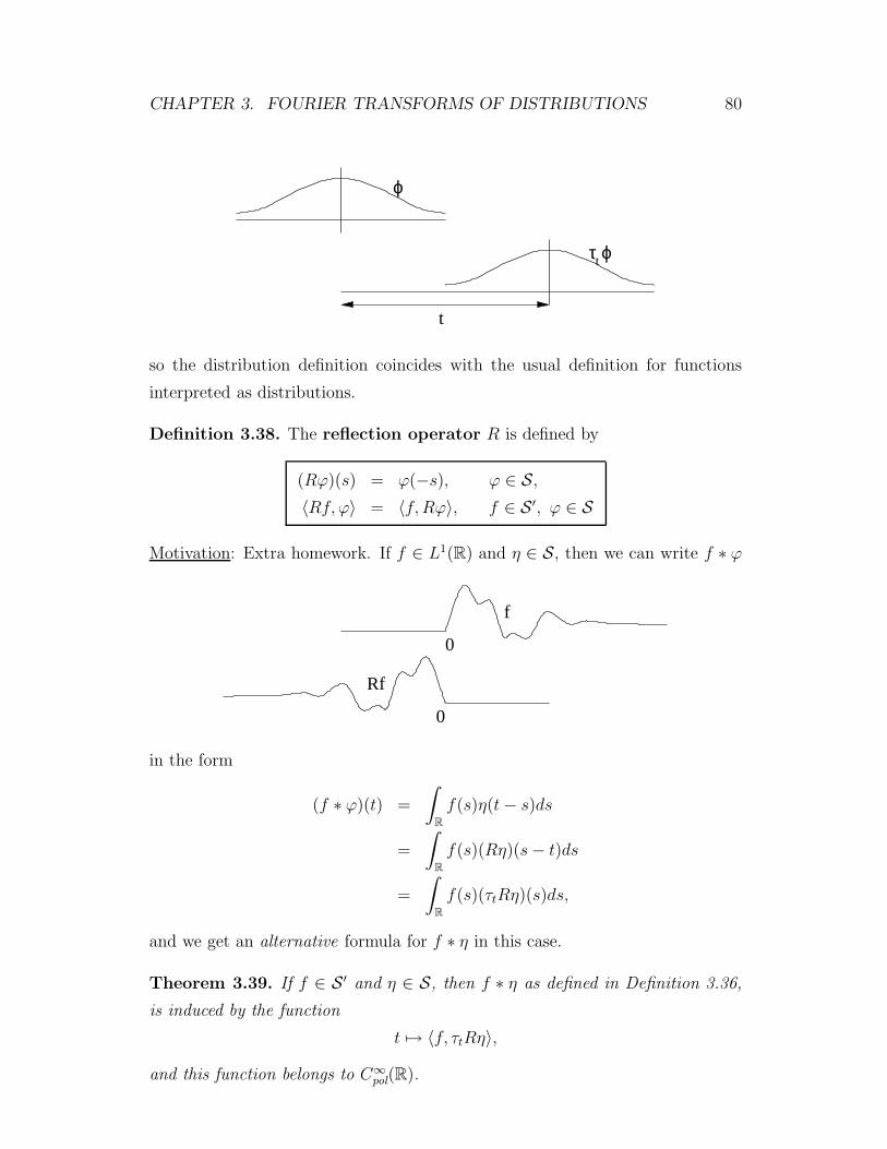
Definition 3.38. The reflection operator R is defined by

(Rϕ)(s) = ϕ(−s), ϕ ∈ S,

〈Rf, ϕ〉 = 〈f, Rϕ〉, f ∈ S ′, ϕ ∈ S

Motivation: Extra homework. If f ∈ L1(R) and η ∈ S, then we can write f ∗ ϕ

0

0

f

Rf

in the form

(f ∗ ϕ)(t) =

∫

R

f(s)η(t− s)ds

=

∫

R

f(s)(Rη)(s− t)ds

=

∫

R

f(s)(τtRη)(s)ds,

and we get an alternative formula for f ∗ η in this case.

Theorem 3.39. If f ∈ S ′ and η ∈ S, then f ∗ η as defined in Definition 3.36,

is induced by the function

t 7→ 〈f, τtRη〉,

and this function belongs to C∞pol(R).


We shall give a partial proof of this theorem (skipping the most complicated

part). It is based on some auxiliary results which will be used later, too.

Lemma 3.40. Let ϕ ∈ S, and let

ϕε(t) =ϕ(t+ ε) − ϕ(t)

ε, t ∈ R.

Then ϕε → ϕ′ in S as ε→ 0.

Proof. (Outline) Must show that

limε→0

supt∈R

|t|k|ϕ(m)ε (t) − ϕ(m+1)(t)| = 0

for all t,m ∈ Z+. By the mean value theorem,

ϕ(m)(t+ ε) = ϕ(m)(t) + εϕ(m+1)(ξ)

where t < ξ < t+ ε (if ε > 0). Thus

|ϕ(m)ε (t) − ϕ(m+1)(t)| = |ϕ(m+1)(ξ) − ϕ(m+1)(t)|

= |

∫ t

ξ

ϕ(m+2)(s)ds|

(where t < ξ < t+ ε if ε > 0

or t+ ε < ξ < t if ε < 0

)

≤

∫ t+|ε|

t−|ε|

|ϕ(m+2)(s)|ds,

and this multiplied by |t|k tends uniformly to zero as ε→ 0. (Here I am skipping

a couple of lines).

Lemma 3.41. For every f ∈ S ′ there exist two numbers M > 0 and N ∈ Z+ so

that

|〈f, ϕ〉| ≤M max0≤j,k≤Nt∈R

|tjϕ(k)(t)|. (3.2)

Interpretation: Every f ∈ S ′ has a finite order (we need only derivatives ϕ(k)

where k ≤ N) and a finite polynomial growth rate (we need only a finite power

tj with j ≤ N).

Proof. Assume to get a contradiction that (3.2) is false. Then for all n ∈ Z+,

there is a function ϕn ∈ S so that

|〈f, ϕn〉| ≥ n max0≤j,k≤nt∈R

|tjϕ(k)n (t)|.


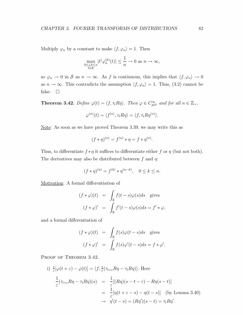
Multiply ϕn by a constant to make 〈f, ϕn〉 = 1. Then

max0≤j,k≤nt∈R

|tjϕ(k)n (t)| ≤

1

n→ 0 as n→ ∞,

so ϕn → 0 in S as n → ∞. As f is continuous, this implies that 〈f, ϕn〉 → 0

as n → ∞. This contradicts the assumption 〈f, ϕn〉 = 1. Thus, (3.2) cannot be

false.

Theorem 3.42. Define ϕ(t) = 〈f, τtRη〉. Then ϕ ∈ C∞pol, and for all n ∈ Z+,

ϕ(n)(t) = 〈f (n), τtRη〉 = 〈f, τtRη(n)〉.

Note: As soon as we have proved Theorem 3.39, we may write this as

(f ∗ η)(n) = f (n) ∗ η = f ∗ η(n).

Thus, to differentiate f ∗η it suffices to differentiate either f or η (but not both).

The derivatives may also be distributed between f and η:

(f ∗ η)(n) = f (k) ∗ η(n−k), 0 ≤ k ≤ n.

Motivation: A formal differentiation of

(f ∗ ϕ)(t) =

∫

R

f(t− s)ϕ(s)ds gives

(f ∗ ϕ)′ =

∫

R

f ′(t− s)ϕ(s)ds = f ′ ∗ ϕ,

and a formal differentiation of

(f ∗ ϕ)(t) =

∫

R

f(s)ϕ(t− s)ds gives

(f ∗ ϕ)′ =

∫

R

f(s)ϕ′(t− s)ds = f ∗ ϕ′.

Proof of Theorem 3.42.

i) 1ε[ϕ(t+ ε) − ϕ(t)] = 〈f, 1

ε(τt+εRη − τtRη)〉. Here

1

ε(τt+εRη − τtRη)(s) =

1

ε[(Rη)(s− t− ε) − Rη(s− t)]

=1

ε[η(t+ ε− s) − η(t− s)] (by Lemma 3.40)

→ η′(t− s) = (Rη′)(s− t) = τtRη′.


Thus, the following limit exists:

limε→0

1

ε[ϕ(t+ ε) − ϕ(t)] = 〈f, τtRη

′〉.

Repeating the same argument n times we find that ϕ is n times differen-

tiable, and that

ϕ(n) = 〈f, τtRη(n)〉

(or written differently, (f ∗ η)(n) = f ∗ η(n).)

ii) A direct computation shows: If we put

ψ(s) = η(t− s) = (Rη)(s− t) = (τtRη)(s),

then ψ′(s) = −η′(t − s) = −τtRη′. Thus 〈f, τtRη

′〉 = −〈f, ψ′〉 = 〈f ′, ψ〉 =

〈f ′, τtRη〉 (by the definition of distributed derivative). Thus, ϕ′ = 〈f, τtRη′〉 =

〈f ′, τtRη〉 (or written differently, f ∗ η′ = f ′ ∗ η). Repeating this n times

we get

f ∗ η(n) = f (n) ∗ η.

iii) The estimate which shows that ϕ ∈ C∞pol: By Lemma 3.41,

|ϕ(n)(t)| = |〈f (n), τtRη〉|

≤ M max0≤j,k≤Ns∈R

|sj(τtRη)(k)(s)| (ψ as above)

= M max0≤j,k≤Ns∈R

|sjη(k)(t− s)| (t− s = v)

= M max0≤j,k≤Nv∈R

|(t− v)jη(k)(s)|

≤ a polynomial in |t|.

To prove Theorem 3.39 it suffices to prove the following lemma (if two distribu-

tions have the same Fourier transform, then they are equal):

Lemma 3.43. Define ϕ(t) = 〈f, τtRη〉. Then ϕ = f η.

Proof. (Outline) By the distribution definition of ϕ:

〈ϕ, ψ〉 = 〈ϕ, ψ〉 for all ψ ∈ S.


We compute this:

〈ϕ, ψ〉 =

∫ ∞

−∞

ϕ(s)︸︷︷︸functionin C∞

pol

ψ(s)ds

=

∫ ∞

−∞

〈f, τsRη〉ψ(s)ds

= (this step is too difficult : To show that we may move

the integral to the other side of f requires more theory

then we have time to present)

= 〈f,

∫ ∞

−∞

τsRηϕ(s)ds〉 = (⋆)

Here τsRη is the function

(τsRη)(t) = (Rη)(t− s) = η(s− t) = (τtη)(s),

so the integral is∫ ∞

−∞

η(s− t)ψ(s)ds =

∫ ∞

−∞

(τtη)(s)ψ(s)ds (see page 43)

=

∫ ∞

−∞

(τtη)(s)ψ(s)ds (see page 38)

=

∫ ∞

−∞

e−2πitsη(s)ψ(s)ds

︸︷︷︸F-transform of ηψ

(⋆) = 〈f, ηψ〉 = 〈f , ηψ〉

= 〈f η, ψ〉. Thus, ϕ = f η.

Using this result it is easy to prove:

Theorem 3.44. Let f ∈ S ′, ϕ, ψ ∈ S. Then

(f ∗ ϕ)︸︷︷︸in C∞

pol

∗ ψ︸︷︷︸in S

︸︷︷︸in C∞

pol

= f︸︷︷︸in S′

∗ (ϕ ∗ ψ)︸︷︷︸in S︸︷︷︸

in C∞

pol

Proof. Take the Fourier transforms:

(f ∗ ϕ)︸︷︷︸↓

f ϕ

∗ ψ︸︷︷︸↓

ψ︸︷︷︸(f ϕ)ψ

= f︸︷︷︸↓

f

∗ (ϕ ∗ ψ)︸︷︷︸↓

ϕψ︸︷︷︸f(ϕψ)

.


The transforms are the same, hence so are the original distributions (note that

both (f ∗ϕ) ∗ψ and f ∗ (ϕ ∗ψ) are in C∞pol so we are allowed to take distribution

Fourier transforms).

3.8 Convergence in S ′

We define convergence in S ′ by means of test functions in S. (This is a special

case of “weak” or “weak*”-convergence).

Definition 3.45. fn → f in S ′ means that

〈fn, ϕ〉 → 〈f, ϕ〉 for all ϕ ∈ S.

Lemma 3.46. Let η ∈ S with η(0) = 1, and define ηλ(t) = λη(λt), t ∈ R, λ > 0.

Then, for all ϕ ∈ S,

ηλ ∗ ϕ→ ϕ in S as λ→ ∞.

Note: We had this type of ”δ-sequences” also in the L1-theory on page 36.

Proof. (Outline.) The Fourier transform is continuous S → S (which we have

not proved, but it is true). Therefore

ηλ ∗ ϕ→ ϕ in S ⇐⇒ ηλ ∗ ϕ→ ϕ in S

⇐⇒ ηλϕ→ ϕ in S

⇐⇒ η(ω/λ)ϕ(ω) → ϕ(ω) in S as λ→ ∞.

Thus, we must show that

supω∈R

∣∣∣ωk(d

dω

)j[η(ω/λ) − 1]ϕ(ω)

∣∣∣→ 0 as λ→ ∞.

This is a “straightforward” mechanical computation (which does take some time).

Theorem 3.47. Define ηλ as in Lemma 3.46. Then

ηλ → δ in S ′ as λ→ ∞.

Comment: This is the reason for the name ”δ-sequence”.

Proof. The claim (=”pastaende”) is that for all ϕ ∈ S,∫

R

ηλ(t)ϕ(t)dt→ 〈δ, ϕ〉 = ϕ(0) as λ→ ∞.


(Or equivalently,∫Rλη(λt)ϕ(t)dt→ ϕ(0) as λ→ ∞). Rewrite this as

∫

R

ηλ(t)(Rϕ)(−t)dt = (ηλ ∗Rϕ)(0),

and by Lemma 3.46, this tends to (Rϕ)(0) = ϕ(0) as λ→ ∞. Thus,

〈ηλ, ϕ〉 → 〈δ, ϕ〉 for all ϕ ∈ S as λ→ ∞,

so ηλ → δ in S ′.

Theorem 3.48. Define ηλ as in Lemma 3.46. Then, for all f ∈ S ′, we have

ηλ ∗ f → f in S ′ as λ→ ∞.

Proof. The claim is that

〈ηλ ∗ f, ϕ〉 → 〈f, ϕ〉 for all ϕ ∈ S.

Replace ϕ with the reflected

ψ = Rϕ =⇒ 〈ηλ ∗ f, Rψ〉 → 〈f, Rψ〉 for all ϕ ∈ S

⇐⇒ (by Thm 3.39) ((ηλ ∗ f) ∗ ψ)(0) → (f ∗ ψ)(0) (use Thm 3.44)

⇐⇒ f ∗ (ηλ ∗ ψ)(0) → (f ∗ ψ)(0) (use Thm 3.39)

⇐⇒ 〈f, R(ηλ ∗ ψ)〉 → 〈f, Rψ〉.

This is true because f is continuous and ηλ ∗ ψ → ψ in S, according to Lemma

3.46.

There is a General Rule about distributions:

Metatheorem: All reasonable claims about distribution convergence are true.

Problem: What is “reasonable”?

Among others, the following results are reasonable:

Theorem 3.49. All the operations on distributions and test functions which we

have defined are continuous. Thus, if

fn → f in S ′, gn → g in S ′,

ψn → ψ in C∞pol (which we have not defined!),

ϕn → ϕ in S,

λn → λ in C, then, among others,


i) fn + gn → f + g in S ′

ii) λnfn → λf in S ′

iii) ψnfn → ψf in S ′

iv) ψn ∗ fn → ψ ∗ f in S ′ (ψ =inverse F-transform of ψ)

v) ϕn ∗ fn → ϕ ∗ f in C∞pol

vi) f ′n → f ′ in S ′

vii) fn → f in S ′ etc.

Proof. “Easy” but long.

3.9 Distribution Solutions of ODE:s

Example 3.50. Find the function u ∈ L2(R+) ∩ C1(R+) with an “absolutely

continuous” derivative u′ which satisfies the equation

u′′(x) − u(x) = f(x), x > 0,

u(0) = 1.

Here f ∈ L2(R+) is given.

Solution. Let v be the solution of homework 22. Thenv′′(x) − v(x) = f(x), x > 0,

v(0) = 0.(3.3)

Define w = u− v. Then w is a solution ofw′′(x) − w(x) = 0, x ≥ 0,

w(0) = 1.(3.4)

In addition we require w ∈ L2(R+).

Elementary solution. The characteristic equation is

λ2 − 1 = 0, roots λ = ±1,

general solution

w(x) = c1ex + c2e

−x.


The condition w(x) ∈ L2(R+) forces c1 = 0. The condition w(0) = 1 gives

w(0) = c2e0 = c2 = 1. Thus: w(x) = e−x, x ≥ 0.

Original solution: u(x) = e−x + v(x), where v is a solution of homework 22, i.e.,

u(x) = e−x +1

2e−x

∫ ∞

0

e−yf(y)dy −1

2

∫ ∞

0

e−|x−y|f(y)dy.

Distribution solution. Make w an even function, and differentiate: we

denote the distribution derivatives by w(1) and w(2). Then

w(1) = w′ (since w is continuous at zero)

w(2) = w′′ + 2w′(0)︸︷︷︸due to jumpdiscontinuityat zero in w′

δ0 (Dirac delta at the point zero)

The problem says: w′′ = w, so

w(2) − w = 2w′(0)δ0. Transform:

((2πiγ)2 − 1)w(γ) = 2w′(0) (since δ0 ≡ 1)

=⇒ w(γ) = 2w′(0)1+4π2γ2 ,

whose inverse transform is −w′(0)e−|x| (see page 62). We are only interested in

values x ≥ 0 so

w(x) = −w′(0)e−x, x > 0.

The condition w(0) = 1 gives −w′(0) = 1, so

w(x) = e−x, x ≥ 0.

Example 3.51. Solve the equation

u′′(x) − u(x) = f(x), x > 0,

u′(0) = a,

where a =given constant, f(x) given function.

Many different ways exist to attack this problem:

Method 1. Split u in two parts: u = v + w, where

v′′(x) − v(x) = f(x), x > 0

v′(0) = 0,


and w′′(x) − w(x) = 0, x > 0

w′(0) = a,

We can solve the first equation by making an even extension of v. The second

equation can be solved as above.

Method 2. Make an even extension of u and transform. Let u(1) and u(2) be

the distribution derivatives of u. Then as above,

u(1) = u′ (u is continuous)

u(2) = u′′ + 2 u′(0)︸︷︷︸=a

δ0 (u′ discontinuous)

By the equation: u′′ = u+ f , so

u(2) − u = 2aδ0 + f

Transform this:[(2πiγ)2 − 1]u = 2a+ f , so

u = −2a1+4π2γ2 −

f1+4π2γ2

Invert:

u(x) = −ae−|x| −1

2

∫ ∞

−∞

e−|x−y|f(y)dy.

Since f is even, this becomes for x > 0:

u(x) = −ae−x −1

2e−x

∫ ∞

0

e−yf(y)dy −1

2

∫ ∞

0

e−|x−y|f(y)dy.

Method 3. The method to make u and f even or odd works, but it is a “dirty

trick” which has to be memorized. A simpler method is to define u(t) ≡ 0 and

f(t) ≡ 0 for t < 0, and to continue as above. We shall return to this method in

connection with the Laplace transform.

Partial Differential Equations are solved in a similar manner. The computations

become slightly more complicated, and the motivations become much more com-

plicated. For example, we can replace all the functions in the examples on page

63 and 64 by distributions, and the results “stay the same”.

3.10 The Support and Spectrum of a Distribu-

tion

“Support” = “the piece of the real line on which the distribution stands”


Definition 3.52. The support of a continuous function ϕ is the closure (=”slutna

holjet”) of the set x ∈ R : ϕ(x) 6= 0.

Note: The set x ∈ R : ϕ(x) 6= 0 is open, but the support contains, in addition,

the boundary points of this set.

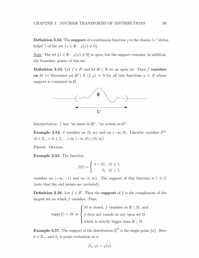
Definition 3.53. Let f ∈ S ′ and let U ⊂ R be an open set. Then f vanishes

on U (=”forsvinner pa U”) if 〈f, ϕ〉 = 0 for all test functions ϕ ∈ S whose

support is contained in U .

U

ϕ

Interpretation: f has “no mass in U”, “no action on U”.

Example 3.54. δ vanishes on (0,∞) and on (−∞, 0). Likewise vanishes δ(k)

(k ∈ Z+ = 0, 1, 2, . . .) on (−∞, 0) ∪ (0,∞).

Proof. Obvious.

Example 3.55. The function

f(t) =

1 − |t|, |t| ≤ 1,

0, |t| > 1,

vanishes on (−∞,−1) and on (1,∞). The support of this function is [−1, 1]

(note that the end points are included).

Definition 3.56. Let f ∈ S ′. Then the support of f is the complement of the

largest set on which f vanishes. Thus,

supp(f) = M ⇔

M is closed, f vanishes on R \M , and

f does not vanish on any open set Ω

which is strictly bigger than R \M .

Example 3.57. The support of the distribution δ(k)a is the single point a. Here

k ∈ Z+, and δa is point evaluation at a:

〈δa, ϕ〉 = ϕ(a).


Definition 3.58. The spectrum of a distribution f ∈ S ′ is the support of f .

Lemma 3.59. If M ⊂ R is closed, then supp(f) ⊂M if and only if f vanishes

on R \M .

Proof. Easy.

Example 3.60. Interpret f(t) = tn as a distribution. Then f = 1(−2πi)n δ

(n), as

we saw on page 78. Thus the support of f is 0, so the spectrum of f is 0.

By adding such functions we get:

Theorem 3.61. The spectrum of the function f(t) ≡ 0 is empty. The spectrum

of every other polynomial is the single point 0.

Proof. f(t) ≡ 0 ⇐⇒ spectrum is empty follows from definition. The other

half is proved above.

The converse is true, but much harder to prove:

Theorem 3.62. If f ∈ S ′ and if the spectrum of f is 0, then f is a polynomial

( 6≡ 0).

This follows from the following theorem by taking Fourier transforms:

Theorem 3.63. If the support of f is one single point a then f can be written

as a finite sum

f =

n∑

k=0

anδ(k)a .

Proof. Too difficult to include. See e.g., Rudin’s “Functional Analysis”.

Possible homework: Show that

Theorem 3.64. The spectrum of f is a ⇐⇒ f(t) = e2πiatP (t), where P is a

polynomial, P 6≡ 0.

Theorem 3.65. Suppose that f ∈ S ′ has a bounded support, i.e., f vanishes on

(−∞,−T ) and on (T,∞) for some T > 0 ( ⇐⇒ supp(f) ⊂ [−T, T ]). Then f

can be interpreted as a function, namely as

f(ω) = 〈f, η(t)e−2πiωt〉,

where η ∈ S is an arbitrary function satifying η(t) ≡ 1 for t ∈ [−T−1, T+1] (or,

more generally, for t ∈ U where U is an open set containing supp(f)). Moreover,

f ∈ C∞pol(R).


Proof. (Not quite complete)

Step 1. Define

ψ(ω) = 〈f, η(t)e−2πiωt〉,

where η is as above. If we choose two different η1 and η2, then η1(t) − η2(t) = 0

is an open set U containing supp(f). Since f vanishes on R\U , we have

〈f, η1(t)e−2πiωt〉 = 〈f, η2(t)e

−2πiωt〉,

so ψ(ω) does not depend on how we choose η.

Step 2. For simplicity, choose η(t) so that η(t) ≡ 0 for |t| > T + 1 (where T as

in the theorem). A “simple” but boring computation shows that

1

ε[e−2πi(ω+ε)t − e−2πiωt]η(t) →

∂

∂ωe−2πiωtη(t) = −2πite−2πiωtη(t)

in S as ε → 0 (all derivatives converge uniformly on [−T−1, T+1], and everything

is ≡ 0 outside this interval). Since we have convergence in S, also the following

limit exists:

limε→0

1

ε(ψ(ω + ε) − ψ(ω)) = ψ′(ω)

= limε→0

〈f,1

ε(e−2πi(ω+ε)t − e−2πiωt)η(t)〉

= 〈f,−2πite−2πiωtη(t)〉.

Repeating the same computation with η replaced by (−2πit)η(t), etc., we find

that ψ is infinitely many times differentiable, and that

ψ(k)(ω) = 〈f, (−2πit)ke−2πiωtη(t)〉, k ∈ Z+. (3.5)

Step 3. Show that the derivatives grow at most polynomially. By Lemma 3.41,

we have

|〈f, ϕ〉| ≤M max0≤t,l≤Nt∈R

|tjϕ(l)(t)|.

Apply this to (3.5) =⇒

|ψ(k)(ω)| ≤ M max0≤j,l≤Nt∈R

∣∣∣tj(d

dt

)l(−2πit)ke−2πiωtη(t)

∣∣∣.

The derivative l = 0 gives a constant independent of ω.

The derivative l = 1 gives a constant times |ω|.


The derivative l = 2 gives a constant times |ω|2, etc.

Thus, |ψ(k)(ω)| ≤ const. x[1 + |w|N ], so ψ ∈ C∞pol.

Step 4. Show that ψ = f . That is, show that∫

R

ψ(ω)ϕ(ω)dω = 〈f , ϕ〉(= 〈f, ϕ〉).

Here we need the same “advanced” step as on page 83:∫

R

ψ(ω)ϕ(ω)dω =

∫

R

〈f, e−2πiωtη(t)ϕ(ω)〉dω

= (why??) = 〈f,

∫

R

e−2πiωtη(t)ϕ(ω)dω〉

= 〈f, η(t)ϕ(t)〉

(since η(t) ≡ 1 in a

neighborhood of supp(f)

)

= 〈f, ϕ〉.

A very short explanation of why “why??” is permitted: Replace the integral by

a Riemann sum, which converges in S, i.e., approximate

∫

R

e−2πiωtϕ(ω)dω = limn→∞

∞∑

k=−∞

e−2πiωktϕ(ωk)1

n,

where ωk = k/n.

3.11 Trigonometric Polynomials

Definition 3.66. A trigonometric polynomial is a sum of the form

ψ(t) =m∑

j=1

cje2πiωjt.

The numbers ωj are called the frequencies of ψ.

Theorem 3.67. If we interpret ψ as a polynomial then the spectrum of ψ is

ω1, ω2, . . . , ωm, i.e., the spectrum consists of the frequencies of the polynomial.

Proof. Follows from homework 27, since supp(δωj) = ωj.

Example 3.68. Find the spectrum of the Weierstrass function

σ(t) =∞∑

k=0

ak cos(2πbkt),

where 0 < a < 1, ab ≥ 1.


To solve this we need the following lemma

Lemma 3.69. Let 0 < a < 1, b > 0. Then

N∑

k=0

ak cos(2πbkt) →

∞∑

k=0

ak cos(2πbkt)

in S ′ as N → ∞.

Proof. Easy. Must show that for all ϕ ∈ S,

∫

R

(N∑

k=0

−

∞∑

k=0

)ak cos(2πbkt)ϕ(t)dt→ 0 as N → ∞.

This is true because

∫

R

∞∑

k=N+1

|ak cos(2πbkt)ϕ(t)|dt ≤

∫

R

∞∑

k=N+1

ak|ϕ(t)|dt

≤

∞∑

k=N+1

ak∫ ∞

−∞

|ϕ(t)|dt

=aN+1

1 − a

∫ ∞

−∞

|ϕ(t)|dt→ 0 as N → ∞.

Solution of 3.68: Since∑N

k=0 →∑∞

k=0 in S ′, also the Fourier transforms converge

in S ′, so to find σ it is enough to find the transform of∑N

k=0 ak cos(2πbkt) and

to let N → ∞. This transform is

δ0 +1

2[a(δb + δ−b) + a2(δ−b2 + δb2) + . . .+ aN (δ−bN + δbN )].

Thus,

σ = δ0 +1

2

∞∑

n=1

an(δ−bn + δbn),

where the sum converges in S ′, and the support of this is 0,±b,±b2,±b3, . . .,

which is also the spectrum of σ.

Example 3.70. Let f be periodic with period 1, and suppose that f ∈ L1(T),

i.e.,∫ 1

0|f(t)|dt <∞. Find the Fourier transform and the spectrum of f .

Solution: (Outline) The inversion formula for the periodic transform says that

f =

∞∑

n=−∞

f(n)e2πint.


Working as on page 86 (but a little bit harder) we find that the sum converges

in S ′, so we are allowed to take transforms:

f =

∞∑

n=−∞

f(n)δn (converges still in S ′).

Thus, the spectrum of f is n ∈ N : f(n) 6= 0. Compare this to the theory of

Fourier series.

General Conclusion 3.71. The distribution Fourier transform contains all the

other Fourier transforms in this course. A “universal transform”.

3.12 Singular differential equations

Definition 3.72. A linear differential equation of the type

n∑

k=0

aku(k) = f (3.6)

is regular if it has exactly one solution u ∈ S ′ for every f ∈ S ′. Otherwise it is

singular.

Thus: Singular means: For some f ∈ S ′ it has either no solution or more than

one solution.

Example 3.73. The equation u′ = f . Taking f = 0 we get many different so-

lutions, namely u =constant (different constants give different solutions). Thus,

this equation is singular.

Example 3.74. We saw earlier on page 59-63 that if we work with L2-functions

instead of distributions, then the equation

u′′ + λu = f

is singular iff λ > 0. The same result is true for distributions:

Theorem 3.75. The equation (3.6) is regular

⇔n∑

k=0

ak(2πiω)k 6= 0 for all ω ∈ R.


Before proving this, let us define

Definition 3.76. The function D(ω) =∑n

k=0 ak(2πiω)k is called the symbol of

(3.6)

Thus: Singular ⇔ the symbol vanishes for some ω ∈ R.

Proof of theorem 3.75. Part 1: Suppose that D(ω) 6= 0 for all ω ∈ R.

Transform (3.6):

n∑

k=0

ak(2πiω)ku = f ⇔ D(ω)u = f .

If D(ω) 6= 0 for all ω, then 1D(ω)

∈ C∞pol, so we can multiply by 1

D(ω):

u =1

D(ω)f ⇔ u = K ∗ f

where K is the inverse distribution Fourier transform of 1D(ω)

. Therefore, (3.6)

has exactly one solution u ∈ S ′ for every f ∈ S ′.

Part 2: Suppose that D(a) = 0 for some a ∈ R. Then

〈Dδa, ϕ〉 = 〈δa, Dϕ〉 = D(a)ϕ(a) = 0.

This is true for all ϕ ∈ S, so Dδa is the zero distribution: Dδa = 0.

⇔

n∑

k=0

ak(2πiω)kδa = 0.

Let v be the inverse transform of δa, i.e.,

v(t) = e2πiat ⇒

n∑

k=0

akv(k) = 0.

Thus, v is one solution of (3.6) with f ≡ 0. Another solution is v ≡ 0. Thus,

(3.6) has at least two different solutions ⇒ the equation is singular.

Definition 3.77. If (3.6) is regular, then we call K =inverse transform of 1D(ω)

the Green’s function of (3.6). (Not defined for singular problems.)

How many solutions does a singular equation have? Find them all! (Solution

later!)


Example 3.78. If f ∈ C(R) (and |f(t)| ≤M(1 + |t|k) for some M and k), then

the equation

u′ = f

has at least the solutions

u(x) =

∫ x

0

f(x)dx+ constant

Does it have more solutions?

Answer: No! Why?

Suppose that u′ = f and v′ = f ⇒ u′−v′ = 0. Transform this ⇒ (2πiω)(u−v) =

0.

Let ϕ be a test function which vanishes in some interval [−ε, ε](⇔ the support

of ϕ is in (−∞,−ε] ∪ [ε,∞)). Then

ψ(ω) =ϕ(ω)

2πiω

is also a test function (it is ≡ 0 in [−ε, ε]), since (2πiω)(u− v) = 0 we get

0 = 〈(2πiω)(u− v), ψ〉

= 〈u− v, 2πiωψ(ω)〉 = 〈u− v, ϕ〉.

Thus, 〈u − v, ϕ〉 = 0 when supp(ϕ) ⊂ (−∞,−ε] ∪ [ε,∞), so by definition,

supp(u− v) ⊂ 0. By theorem 3.63, u− v is a polynomial. The only polynomial

whose derivative is zero is the constant function, so u− v is a constant.

A more sophisticated version of the same argument proves the following theorem:

Theorem 3.79. Suppose that the equation

n∑

k=0

aku(k) = f (3.7)

is singular, and suppose that the symbolD(ω) has exactly r simple zeros ω1, ω2, . . . , ωr.

If the equation (3.7) has a solution v, then every other solution u ∈ S ′ of (3.7)

is of the form

u = v +

r∑

j=1

bje2πiωjt,

where the coefficients bj can be chosen arbitrarily.


Compare this to example 3.78: The symbol of the equation u′ = f is 2πiω, which

has a simple zero at zero.

Comment 3.80. The equation (3.7) always has a distribution solution, for all

f ∈ S ′. This is proved for the equation u′ = f in [GW99, p. 277], and this can

be extended to the general case.

Comment 3.81. A zero ωj of order r ≥ 2 of D gives rise to terms of the type

P (t)e2πiωjt, where P (t) is a polynomial of degree ≤ r − 1.

Chapter 3 Fourier Transforms of...

Documents

Transcript of Chapter 3 Fourier Transforms of...