Edge Detection - University of Toronto · Edge Detection Goal: Detection and Localization of Image...

Edge Detection

Goal: Detection and Localization of Image Edges.

Motivation:

• Significant, often sharp, contrast variations in images caused byillumination, surface markings (albedo), and surface boundaries.These are useful for scene interpretation.

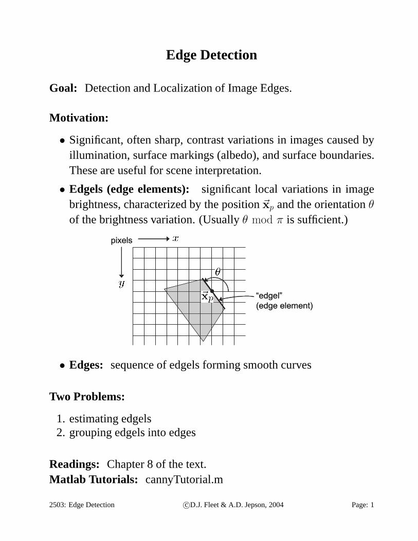
• Edgels (edge elements): significant local variations in imagebrightness, characterized by the position~xp and the orientationθof the brightness variation. (Usuallyθ mod π is sufficient.)

pixels

l“edgel”

(edge element)

pixels

l“edgel”

(edge element)

• Edges: sequence of edgels forming smooth curves

Two Problems:

1. estimating edgels2. grouping edgels into edges

Readings: Chapter 8 of the text.Matlab Tutorials: cannyTutorial.m

2503: Edge Detection c©D.J. Fleet & A.D. Jepson, 2004 Page: 1

1D Ideal Step Edges

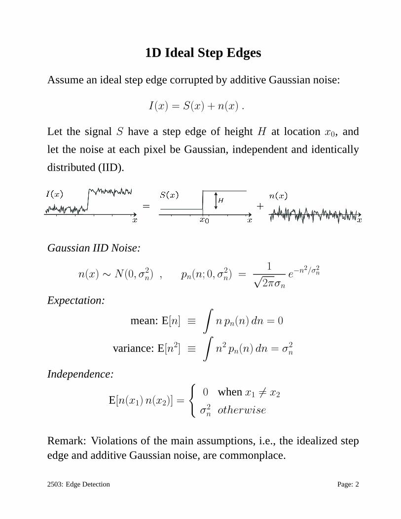
Assume an ideal step edge corrupted by additive Gaussian noise:

I(x) = S(x) + n(x) .

Let the signalS have a step edge of heightH at locationx0, and

let the noise at each pixel be Gaussian, independent and identically

distributed (IID).

Gaussian IID Noise:

n(x) ∼ N(0, σ2n) , pn(n; 0, σ2

n) =1√

2πσn

e−n2/σ2n

Expectation:

mean: E[n] ≡∫

n pn(n) dn = 0

variance: E[n2] ≡∫

n2 pn(n) dn = σ2n

Independence:

E[n(x1) n(x2)] =

{

0 whenx1 6= x2

σ2n otherwise

Remark: Violations of the main assumptions, i.e., the idealized stepedge and additive Gaussian noise, are commonplace.

2503: Edge Detection Page: 2

Optimal Linear Filter

What is the optimal linear filter for the detection and localization of a

step edge in an image?

Assume a linear filter, with impulse responsef(x):

r(x) = f(x) ∗ I(x) = f(x) ∗ S(x) + f(x) ∗ n(x)

= rS(x) + rn(x)

So the response is the sum of responses to the signal and the noise.

The mean and variance of the response to noisern(x),

rn(x) =K∑

k=−K

f(−k) n(x + k) ,

whereK is the radius of filter support, are easily shown to be

E[rn(x)] =∑

k

f(−k) E[n(x + k)] = 0

E[r2n(x)] =

∑

k

∑

l

f(−l) f(−k) E[n(x+k)n(x+l)] = σ2n

∑

k

f 2(k)

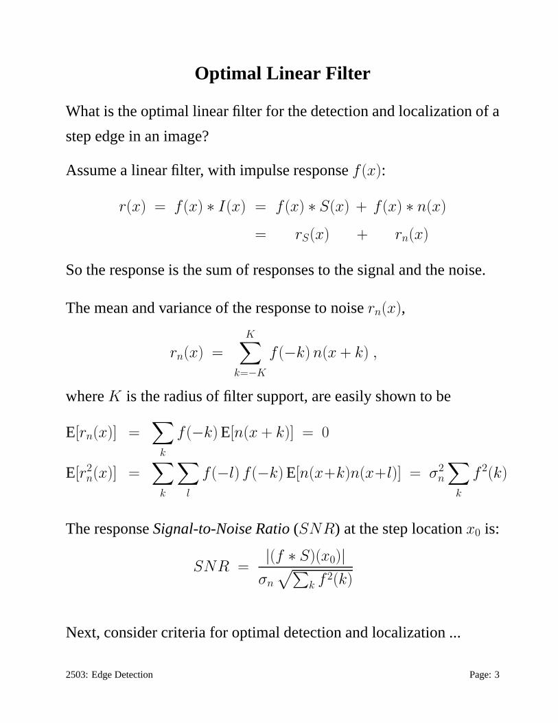
The responseSignal-to-Noise Ratio (SNR) at the step locationx0 is:

SNR =|(f ∗ S)(x0)|

σn

√∑

k f 2(k)

Next, consider criteria for optimal detection and localization ...


Criteria for Optimal Filters

Criterion 1: Good Detection. Choose the filter to maximize the the

SNR of the response at the edge location, subject to constraint that

the responses to constant sigals are zero.

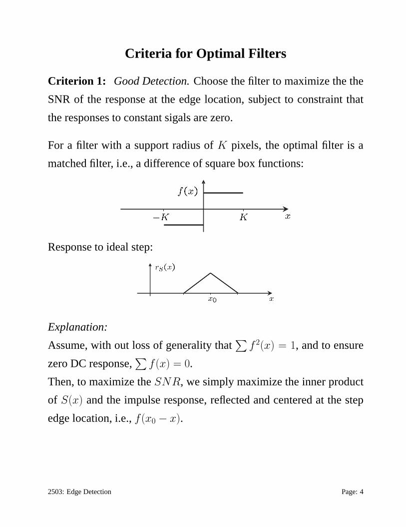
For a filter with a support radius ofK pixels, the optimal filter is a

matched filter, i.e., a difference of square box functions:

Response to ideal step:

Explanation:

Assume, with out loss of generality that∑

f 2(x) = 1, and to ensure

zero DC response,∑

f(x) = 0.

Then, to maximize theSNR, we simply maximize the inner product

of S(x) and the impulse response, reflected and centered at the step

edge location, i.e.,f(x0 − x).


Criteria for Optimal Filters (cont)

Criterion 2: Good Localization. Let {x∗l }L

l=1 be the local maxima

in response magnitude|r(x)|. Choose the filter to minimze the root

mean squared error between thetrue edge location and theclosest

peak in |r|; i.e., minmize

LOC =1

√

E[ mink |x∗l − x0|2 ]

Caveat: for an optimal filter this does not mean that the closest peak

should be the most significant peak, or even readily identifiable.

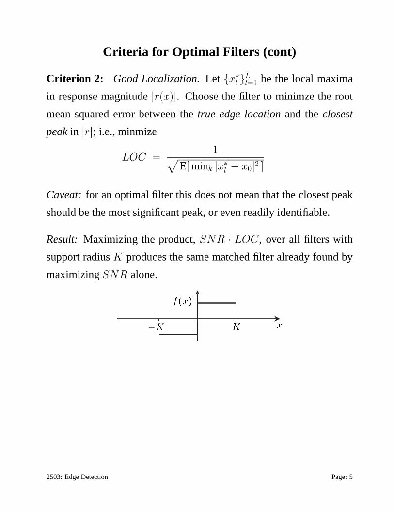
Result: Maximizing the product,SNR · LOC, over all filters with

support radiusK produces the same matched filter already found by

maximizingSNR alone.


Criteria for Optimal Filters (cont)

Criterion 3: Sparse Peaks. MaximizeSNR · LOC, subject to the

constraint that peaks in|r(x)| be as far apart, on average, as a manu-

ally selected constant,xPeak:

E[ |x∗k+1 − x∗

k| ] = xPeak

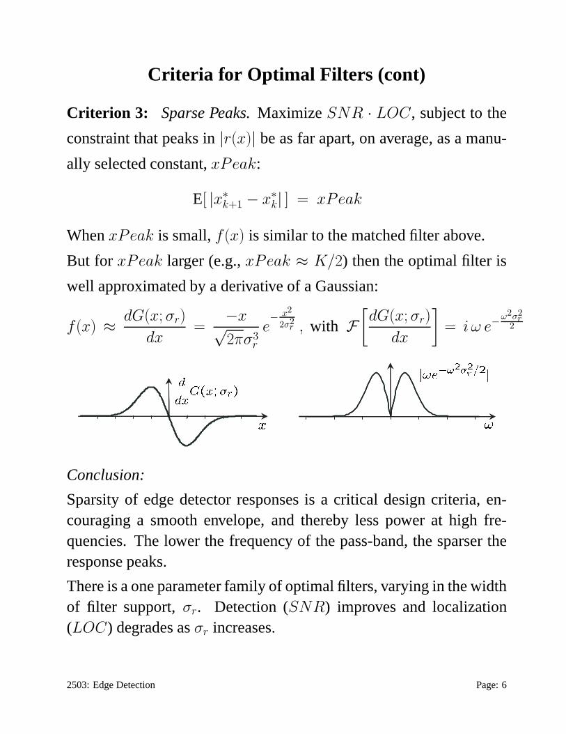
WhenxPeak is small,f(x) is similar to the matched filter above.

But for xPeak larger (e.g.,xPeak ≈ K/2) then the optimal filter is

well approximated by a derivative of a Gaussian:

f(x) ≈ dG(x; σr)

dx=

−x√2πσ3

r

e− x

2

2σ2r , with F

[

dG(x; σr)

dx

]

= i ω e−ω2σ2r

2

Conclusion:

Sparsity of edge detector responses is a critical design criteria, en-couraging a smooth envelope, and thereby less power at high fre-quencies. The lower the frequency of the pass-band, the sparser theresponse peaks.

There is a one parameter family of optimal filters, varying inthe widthof filter support,σr. Detection (SNR) improves and localization(LOC) degrades asσr increases.


Multiscale Edge Features

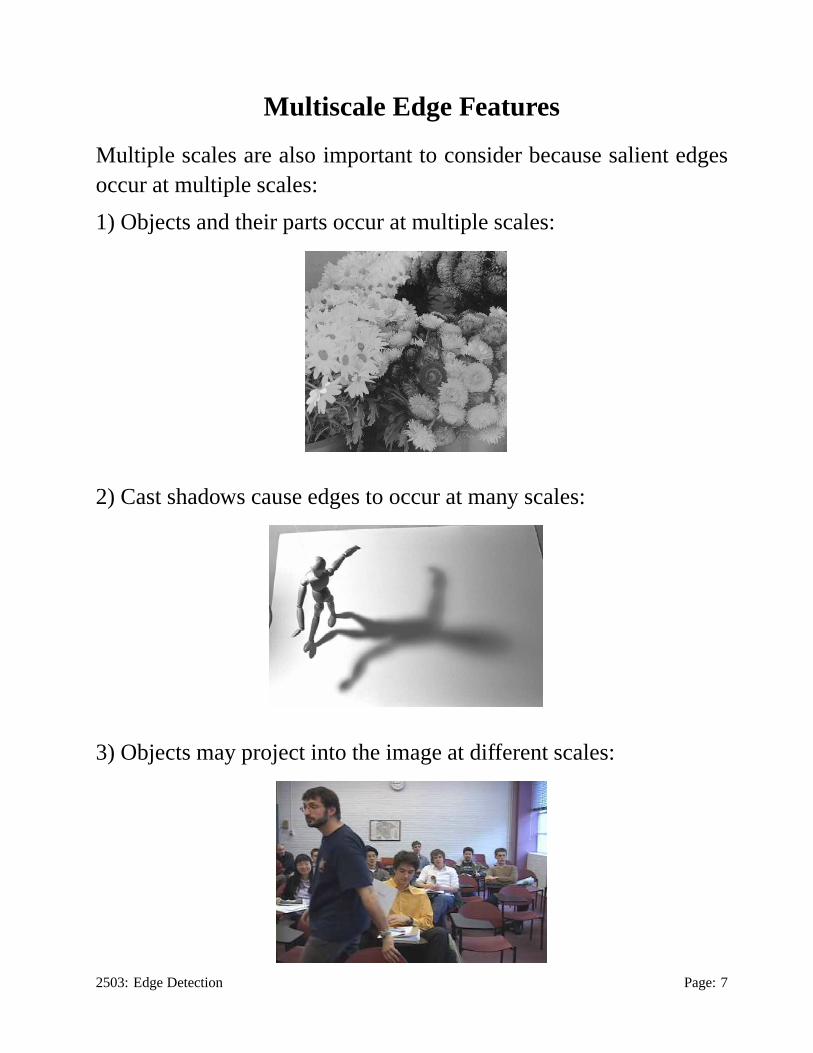
Multiple scales are also important to consider because salient edgesoccur at multiple scales:

1) Objects and their parts occur at multiple scales:

2) Cast shadows cause edges to occur at many scales:

3) Objects may project into the image at different scales:


2D Edge Detection

The corresponding 2D edge detector is based on the magnitudeof the

directional derivative of the image in the direction normalto the edge.

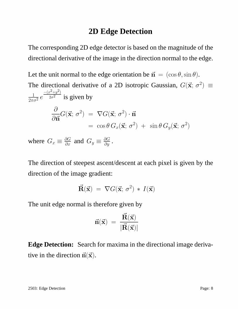
Let the unit normal to the edge orientation be~n = (cos θ, sin θ).

The directional derivative of a 2D isotropic Gaussian,G(~x; σ2) ≡1

2πσ2 e−(x2+y

2)

2σ2 is given by

∂

∂~nG(~x; σ2) = ∇G(~x; σ2) · ~n

= cos θ Gx(~x; σ2) + sin θ Gy(~x; σ2)

whereGx ≡ ∂G∂x

and Gy ≡ ∂G∂y

.

The direction of steepest ascent/descent at each pixel is given by the

direction of the image gradient:

~R(~x) = ∇G(~x; σ2) ∗ I(~x)

The unit edge normal is therefore given by

~n(~x) =~R(~x)

|~R(~x)|

Edge Detection: Search for maxima in the directional image deriva-

tive in the direction~n(~x).


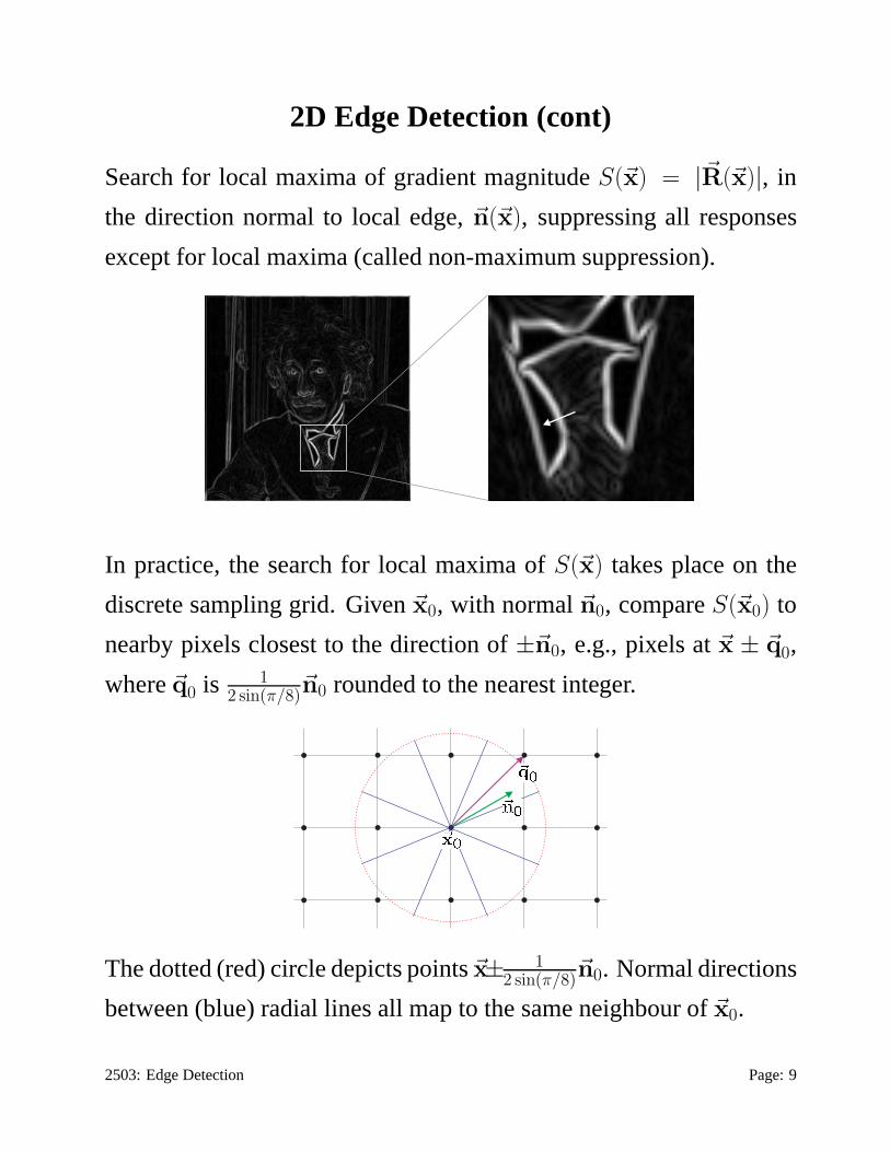
2D Edge Detection (cont)

Search for local maxima of gradient magnitudeS(~x) = |~R(~x)|, in

the direction normal to local edge,~n(~x), suppressing all responses

except for local maxima (called non-maximum suppression).

In practice, the search for local maxima ofS(~x) takes place on the

discrete sampling grid. Given~x0, with normal~n0, compareS(~x0) to

nearby pixels closest to the direction of±~n0, e.g., pixels at~x ± ~q0,

where~q0 is 12 sin(π/8)

~n0 rounded to the nearest integer.

l l

l l

l

l l l

l l l

l l l l

The dotted (red) circle depicts points~x± 12 sin(π/8)

~n0. Normal directions

between (blue) radial lines all map to the same neighbour of~x0.


Canny Edge Detection

Algorithm:

1. Convolve with gradient filters (at multiple scales)

~R(~x) ≡ (Rx(~x), Ry(~x) ) = ∇G(~x; σ2) ∗ I(~x) .

2. Compute response magnitude,S(~x) =√

R2x(~x) + R2

y(~x) .

3. Compute local edge orientation (represented by unit normal):

~n(~x) =

{

(Rx(~x), Ry(~x))/S(~x) if S(~x) > threshold

0 otherwise

4. Peak detection (non-maximum suppression along edge normal)

5. Non-maximum suppression through scale, and hysteresis thresh-

olding along edges (see Canny (1986) for details).

Implementation Remarks:

Separability: Partial derivatives of an isotropic Gaussian:

∂

∂xG(~x; σ2) = − x

σ2G(x; σ2) G(y; σ2) .

Filter Support: In practice, it’s good to sample the impulse response

so that the support radiusK ≥ 3σr. Common values forK are 7, 9,

and 11 (i.e., forσ ≈ 1, 4/3, and5/3).


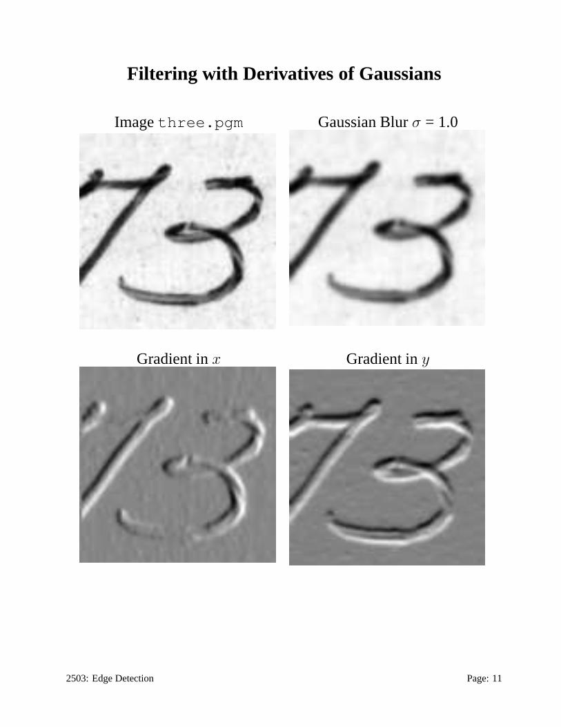
Filtering with Derivatives of Gaussians

Imagethree.pgm Gaussian Blurσ = 1.0

Gradient inx Gradient iny


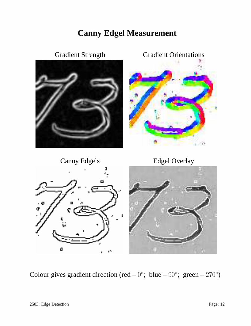
Canny Edgel Measurement

Gradient Strength Gradient Orientations

Canny Edgels Edgel Overlay

Colour gives gradient direction (red –0◦; blue –90◦; green –270◦)


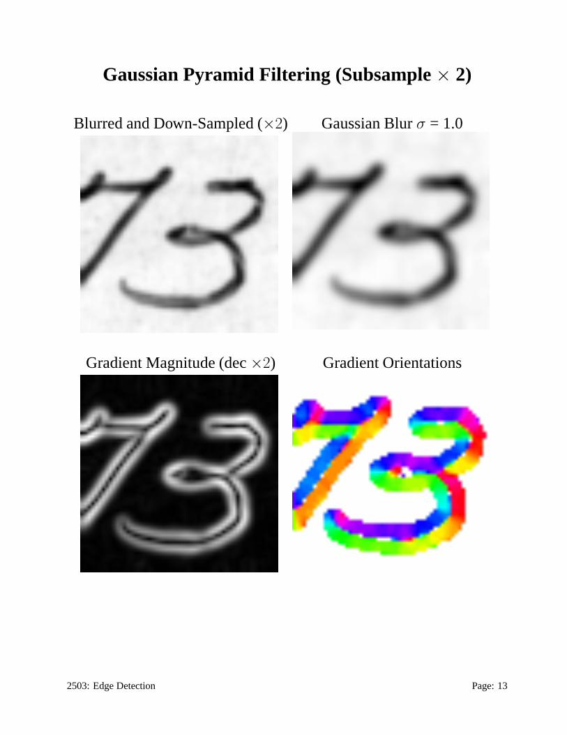
Gaussian Pyramid Filtering (Subsample× 2)

Blurred and Down-Sampled (×2) Gaussian Blurσ = 1.0

Gradient Magnitude (dec×2) Gradient Orientations


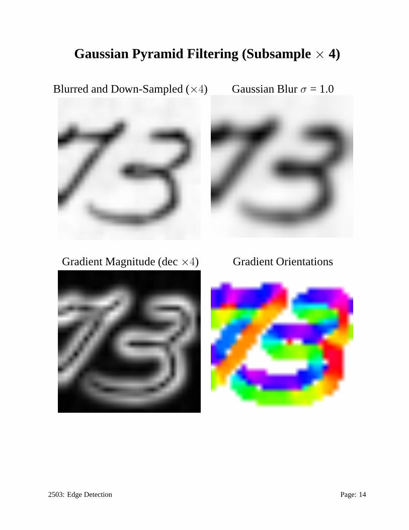
Gaussian Pyramid Filtering (Subsample× 4)

Blurred and Down-Sampled (×4) Gaussian Blurσ = 1.0

Gradient Magnitude (dec×4) Gradient Orientations


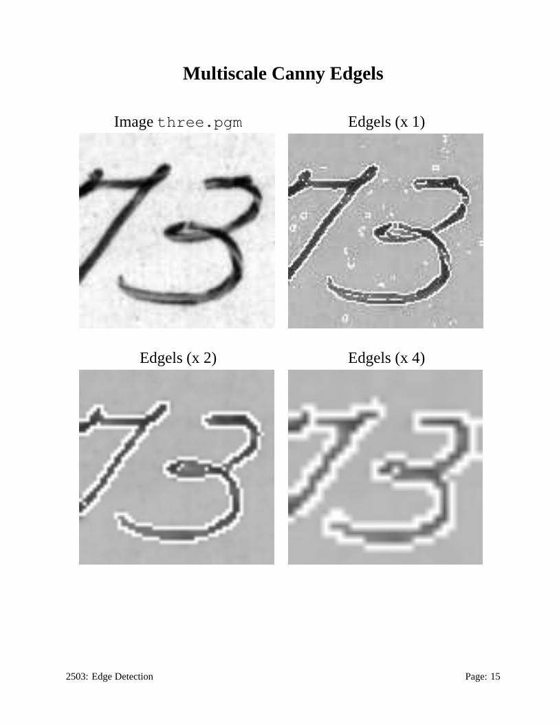
Multiscale Canny Edgels

Imagethree.pgm Edgels (x 1)

Edgels (x 2) Edgels (x 4)


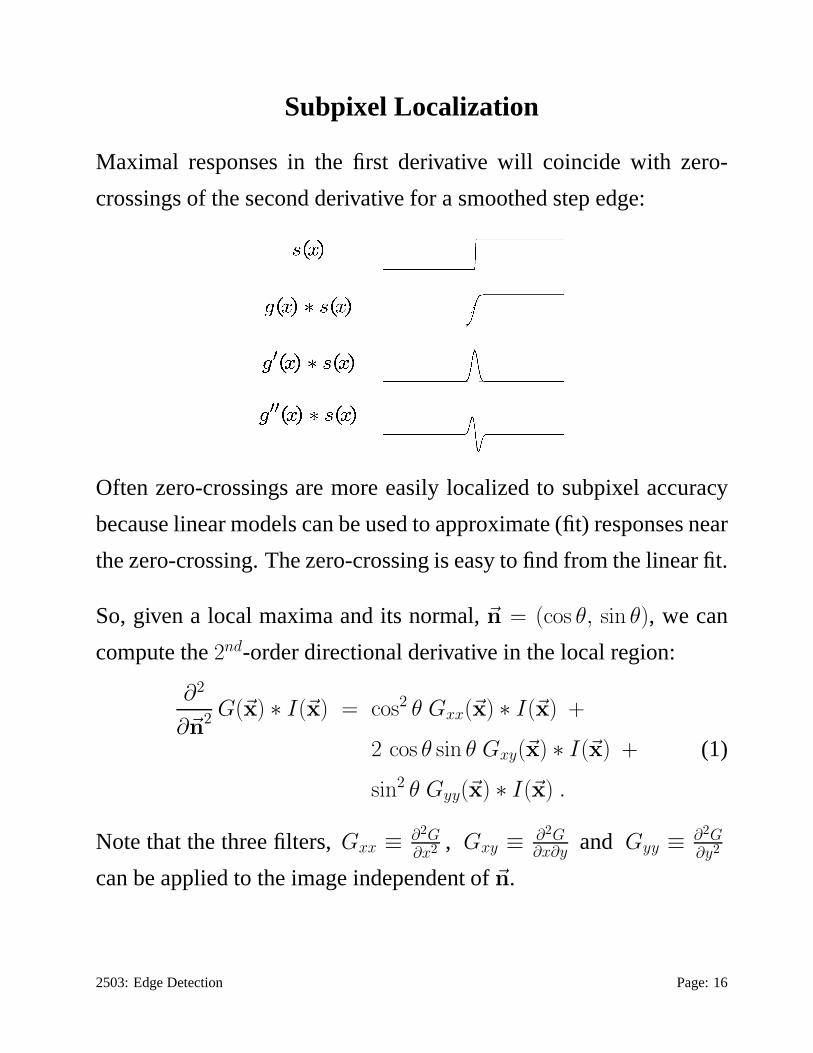
Subpixel Localization

Maximal responses in the first derivative will coincide withzero-

crossings of the second derivative for a smoothed step edge:

Often zero-crossings are more easily localized to subpixelaccuracy

because linear models can be used to approximate (fit) responses near

the zero-crossing. The zero-crossing is easy to find from thelinear fit.

So, given a local maxima and its normal,~n = (cos θ, sin θ), we can

compute the2nd-order directional derivative in the local region:

∂2

∂~n2 G(~x) ∗ I(~x) = cos2 θ Gxx(~x) ∗ I(~x) +

2 cos θ sin θ Gxy(~x) ∗ I(~x) + (1)

sin2 θ Gyy(~x) ∗ I(~x) .

Note that the three filters,Gxx ≡ ∂2G∂x2 , Gxy ≡ ∂2G

∂x∂y and Gyy ≡ ∂2G∂y2

can be applied to the image independent of~n.


Steerable Filters

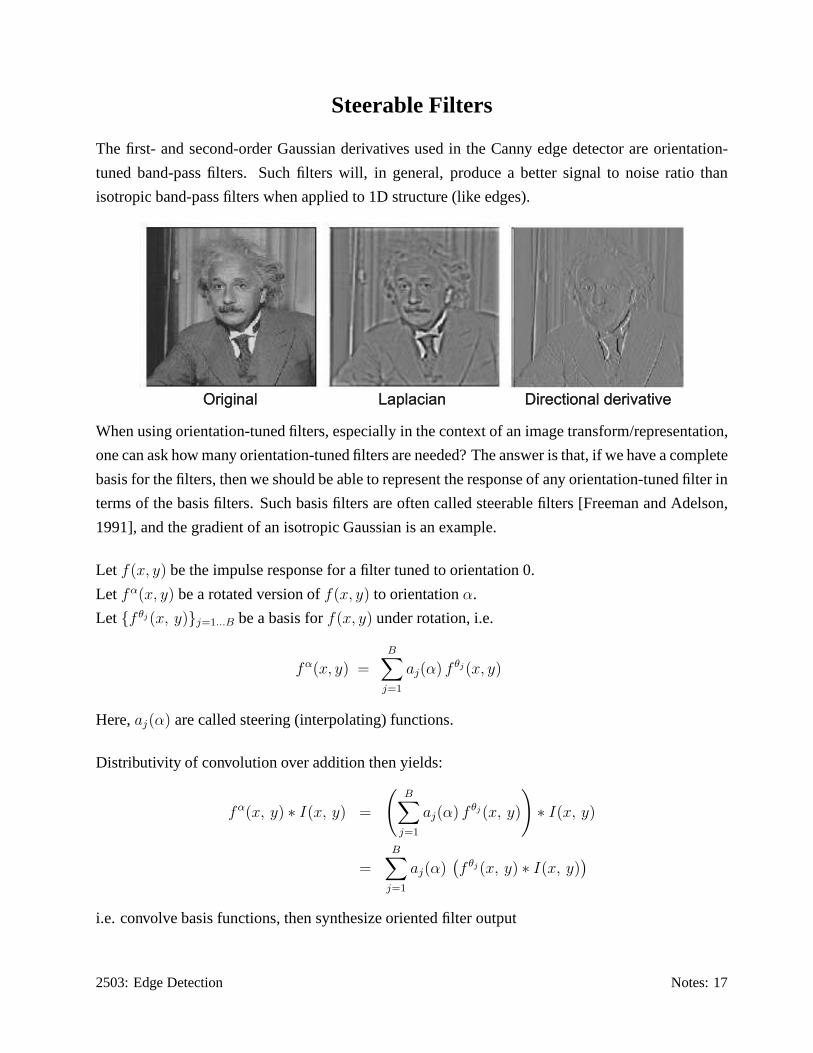
The first- and second-order Gaussian derivatives used in theCanny edge detector are orientation-

tuned band-pass filters. Such filters will, in general, produce a better signal to noise ratio than

isotropic band-pass filters when applied to 1D structure (like edges).

Original Laplacian Directional derivativeOriginal Laplacian Directional derivative

When using orientation-tuned filters, especially in the context of an image transform/representation,

one can ask how many orientation-tuned filters are needed? The answer is that, if we have a complete

basis for the filters, then we should be able to represent the response of any orientation-tuned filter in

terms of the basis filters. Such basis filters are often calledsteerable filters [Freeman and Adelson,

1991], and the gradient of an isotropic Gaussian is an example.

Let f(x, y) be the impulse response for a filter tuned to orientation 0.

Let fα(x, y) be a rotated version off(x, y) to orientationα.

Let {f θj(x, y)}j=1...B be a basis forf(x, y) under rotation, i.e.

fα(x, y) =

B∑

j=1

aj(α) f θj(x, y)

Here,aj(α) are called steering (interpolating) functions.

Distributivity of convolution over addition then yields:

fα(x, y) ∗ I(x, y) =

(

B∑

j=1

aj(α) f θj(x, y)

)

∗ I(x, y)

=

B∑

j=1

aj(α)(

f θj(x, y) ∗ I(x, y))

i.e. convolve basis functions, then synthesize oriented filter output

2503: Edge Detection Notes: 17

Steerable Filters – Directional Derivatives

Consider the directional first derivative of a Gaussian,g(x, y) = e−(x2+y2)/2.

The first derivatives in the horizontal and vertical directions:

gx(x, y) = −x e−(x2+y2)/2 , gy(x, y) = −y e−(x2+y2)/2

General derivative in direction~s = (s1, s2) = (cos(θ), sin(θ))

gs(x, y) = (s1, s2) · (gx(x, y), gy(x, y))

So output of filter tuned to orientationθ is given by

gs(x, y) ∗ I(x, y) = (s1 gx + s2 gy) ∗ I(x, y) = (s1, s2) · (gx ∗ I, gy ∗ I)

Explanation: In polar coordinates, the horizontal Gaussian derivative is:

gx(r, θ) = −r e−r2/2 cos(θ)

which is a polar separable product ofcos(θ) and−r e−r2/2. In polar coordinates it is easy to see that

a rotation byπ/2 is given by

gx(r, θ − π/2) = −re−r2/2 cos(θ − π/2)

= −re−r2/2 sin(θ)

= gy(r, θ)

And in general;, a rotation byθ0, i.e., to direction~s = (cos(θ0), sin(θ0))

gx(r, θ − θ0) = −re−r2/2 cos(θ − θ0)

= −re−r2/2 [cos(θ) cos(θ0) + sin(θ) sin(θ0)]

= cos(θ0) gx + sin(θ0) gy

The same ideas also work with higher-order derivatives, separable polynomial functions, and polar

separable functions having a limited numbers of angular frequency components. For example,

∂2

∂s2g(x, y) =

2∑

k=0

2!

k! (2 − k)!sk

x s2−ky

∂2g(x, y)

∂xk ∂y2−k.

This is precisely the form of the second directional derivative given in Eqn (1), for direction~s.


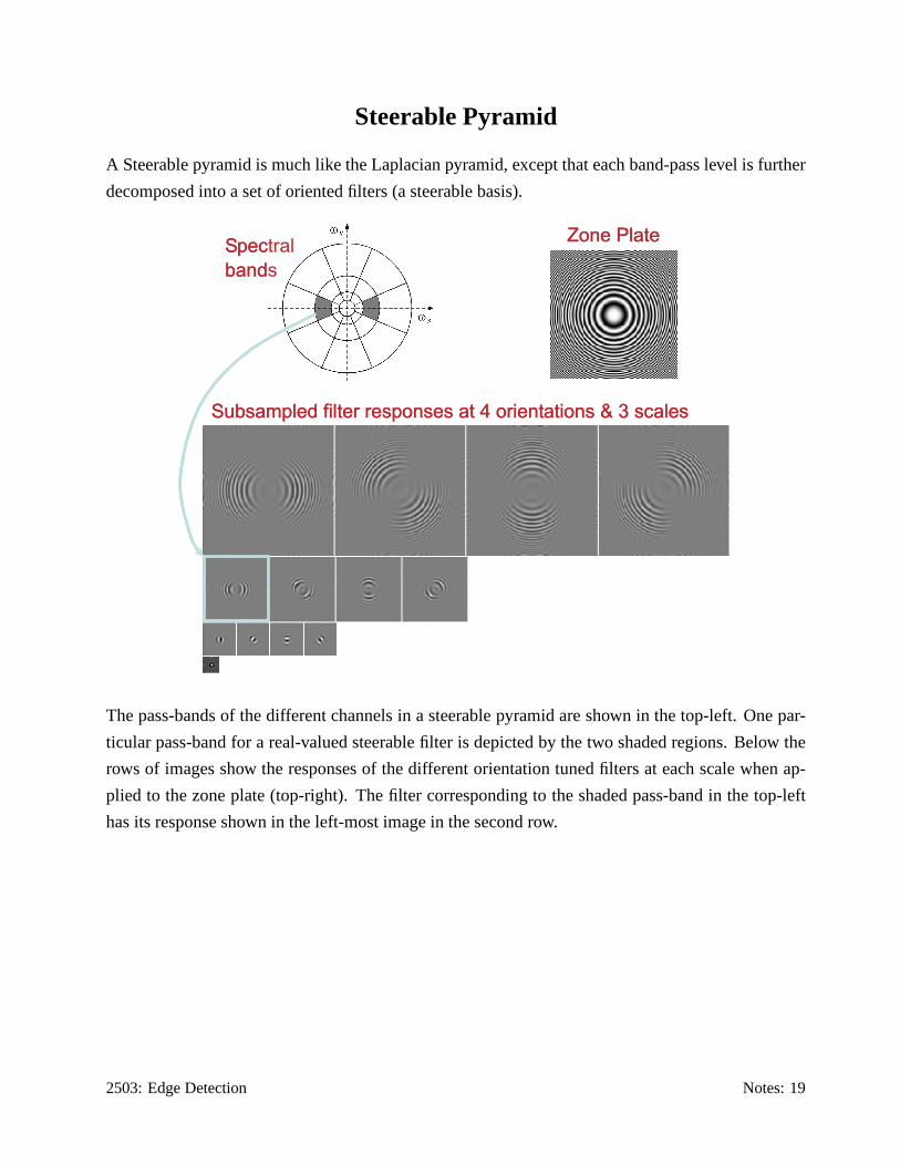
Steerable Pyramid

A Steerable pyramid is much like the Laplacian pyramid, except that each band-pass level is further

decomposed into a set of oriented filters (a steerable basis).

Zone Plate

Subsampled filter responses at 4 orientations & 3 scales

Spectral

bands

Zone Plate

Subsampled filter responses at 4 orientations & 3 scales

Spectral

bands

The pass-bands of the different channels in a steerable pyramid are shown in the top-left. One par-

ticular pass-band for a real-valued steerable filter is depicted by the two shaded regions. Below the

rows of images show the responses of the different orientation tuned filters at each scale when ap-

plied to the zone plate (top-right). The filter corresponding to the shaded pass-band in the top-left

has its response shown in the left-most image in the second row.


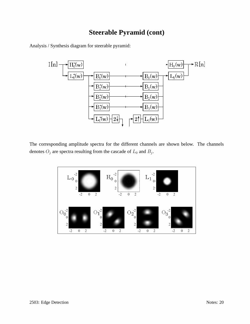
Steerable Pyramid (cont)

Analysis / Synthesis diagram for steerable pyramid:

The corresponding amplitude spectra for the different channels are shown below. The channels

denotesOj are spectra resulting from the cascade ofL0 andBj.

20-2 20-2 20-2

20-2 20-2 20-2 20-2

2

0

-2

2

0

-2

2

0

-2

2

0

-2

2

0

-2

2

0

-2

2

0

-2


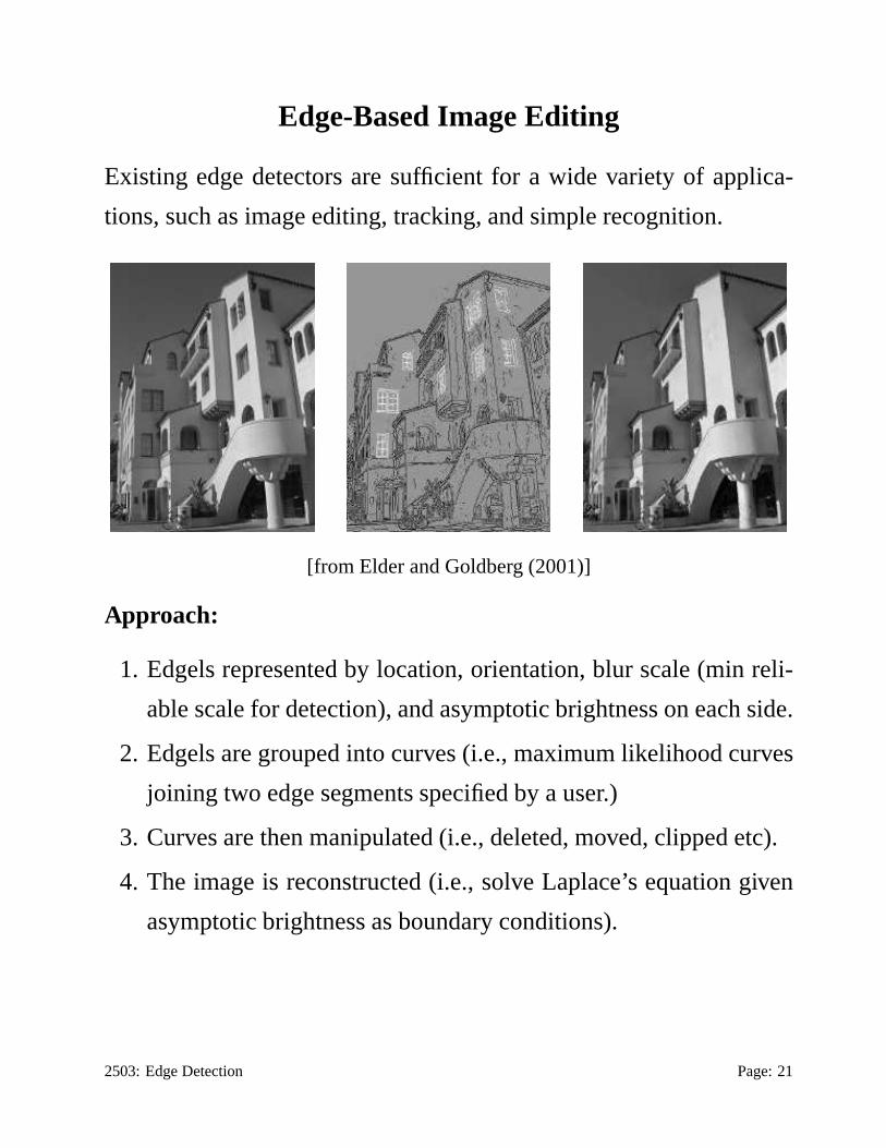
Edge-Based Image Editing

Existing edge detectors are sufficient for a wide variety of applica-

tions, such as image editing, tracking, and simple recognition.

[from Elder and Goldberg (2001)]

Approach:

1. Edgels represented by location, orientation, blur scale(min reli-

able scale for detection), and asymptotic brightness on each side.

2. Edgels are grouped into curves (i.e., maximum likelihoodcurves

joining two edge segments specified by a user.)

3. Curves are then manipulated (i.e., deleted, moved, clipped etc).

4. The image is reconstructed (i.e., solve Laplace’s equation given

asymptotic brightness as boundary conditions).


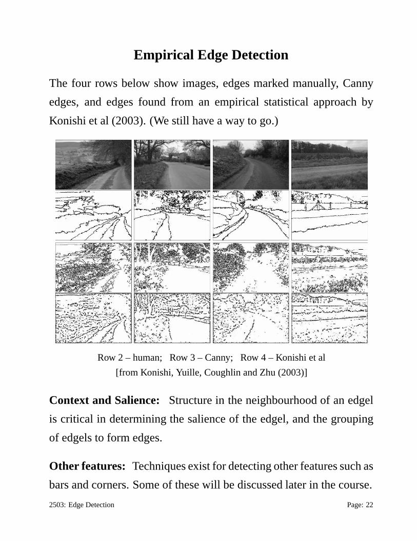
Empirical Edge Detection

The four rows below show images, edges marked manually, Canny

edges, and edges found from an empirical statistical approach by

Konishi et al (2003). (We still have a way to go.)

Row 2 – human; Row 3 – Canny; Row 4 – Konishi et al

[from Konishi, Yuille, Coughlin and Zhu (2003)]

Context and Salience: Structure in the neighbourhood of an edgel

is critical in determining the salience of the edgel, and thegrouping

of edgels to form edges.

Other features: Techniques exist for detecting other features such as

bars and corners. Some of these will be discussed later in thecourse.


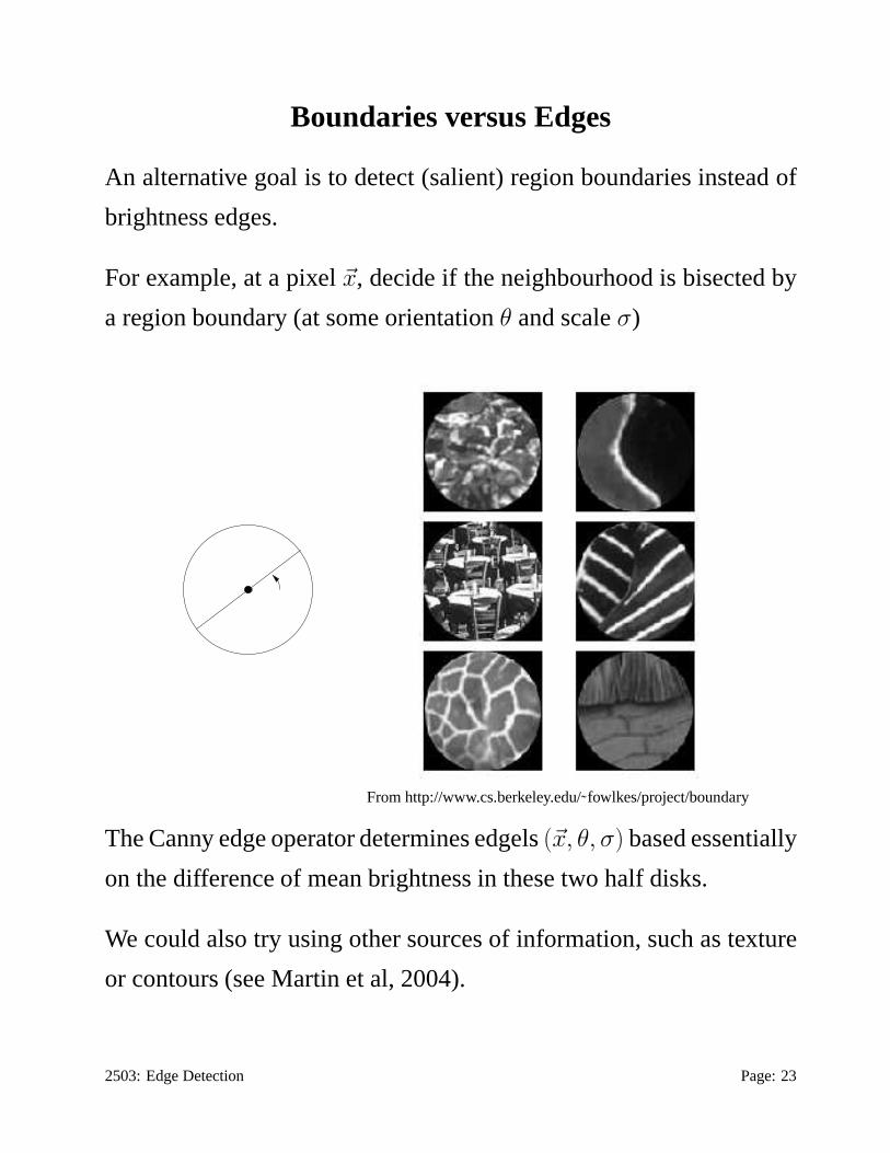
Boundaries versus Edges

An alternative goal is to detect (salient) region boundaries instead of

brightness edges.

For example, at a pixel~x, decide if the neighbourhood is bisected by

a region boundary (at some orientationθ and scaleσ)

From http://www.cs.berkeley.edu/˜fowlkes/project/boundary

The Canny edge operator determines edgels(~x, θ, σ) based essentially

on the difference of mean brightness in these two half disks.

We could also try using other sources of information, such astexture

or contours (see Martin et al, 2004).


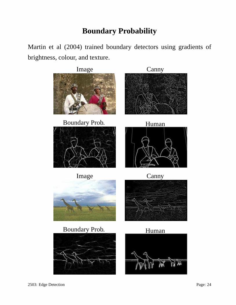
Boundary Probability

Martin et al (2004) trained boundary detectors using gradients of

brightness, colour, and texture.

Image Canny

Boundary Prob. Human

Image Canny

Boundary Prob. Human


Further Readings

Castleman, K.R.,Digital Image Processing, Prentice Hall, 1995

John Canny, ”A computational approach to edge detection.”IEEE Transactions on PAMI, 8(6):679–

698, 1986.

James Elder and Richard Goldberg, ”Image editing in the contour domain.”IEEE Transactions on

PAMI, 23(3):291–296, 2001.

Scott Konishi, Alan Yuille, James Coughlin, and Song Chun Zhu, ”Statistical edge detection:

Learning and evaluating edge cues.”IEEE Transactions on PAMI, 25(1):57–74, 2003.

William Freeman and Edward Adelson, ”The design and use of steerable filters.”IEEE Transac-

tions on PAMI, 13:891–906, 1991.

David Martin, Charless Fowlkes, and Jitendra Malik, ”Learning to detect natural image boundaries

using local brightness, color, and texture cues.”IEEE Transactions on PAMI, 26(5):530–549,

2004.


Edge Detection - University of Toronto · Edge Detection Goal: Detection and Localization of Image...

Documents

Transcript of Edge Detection - University of Toronto · Edge Detection Goal: Detection and Localization of Image...