Serdica Math. J.serdica/2006/2006-099-130.pdf · Serdica Math. J. 32 (2006), 99{130 Lp EXTREMAL...
33
Transcript of Serdica Math. J.serdica/2006/2006-099-130.pdf · Serdica Math. J. 32 (2006), 99{130 Lp EXTREMAL...
Serdica Math. J. 32 (2006), 99–130
Lp EXTREMAL POLYNOMIALS.
RESULTS AND PERSPECTIVES
Yamina Laskri and Rachid Benzine
Communicated by E. Horozov
Abstract. Let α = β+ γ be a positive finite measure defined on the Borelsets of C, with compact support, where β is a measure concentrated on aclosed Jordan curve or on an arc (a circle or a segment) and γ is a discretemeasure concentrated on an infinite number of points.In this survey paper, we present a synthesis on the asymptotic behaviourof orthogonal polynomials or Lp extremal polynomials associated to themeasure α. We analyze some open problems and discuss new ideas relatedto their solving.
1. Introduction. Let α be a positive finite measure defined on theBorel set B(C) of C, with compact support F . The Lp extremal polynomialsTn,p,α associated to the measure α and the support F are defined as the solutions
2000 Mathematics Subject Classification: 30C40, 30D50, 30E10, 30E15, 42C05.Key words: Asymptotic behaviour, orthogonal polynomials, Lp extremal polynomials, curve,
arc, circle, segment.
100 Yamina Laskri and Rachid Benzine
of extremal problems in the space Lp(F, α). Let mn,p(α) (n ∈ N, p > 0) denotethe extremal constants associated with α and F :
mn,p(α) = ‖Tn,p,α‖Lp(F,α)
= min
‖Qn‖Lp(F,α) : Qn = zn + an−1z
n−1 + · · · + a0,
a0, a1, . . . , an−1 ∈ C.
(1)
Let us remark that in the case p = 2, the polynomials Tn,2,α coincide exactly withthe (monic) orthogonal polynomials, and satisfy the following relations
Tn,2,α(z) = zn + · · · ;∫
FTn,2,α(z)Tm,2,α(z)dα(z) = 0; if n 6= m.(2)
Many schools have studied the properties of orthogonal polynomials or Lp extre-mal polynomials, particularly:
a) Schools which are interested with the formal or algebraic case oforthogonal polynomials or Lp extremal polynomials (recurrent properties, thezeros distribution, formal resolution of differential equations, . . . ).
b) Schools which are interested on the analytic or functional case oforthogonal polynomials or Lp extremal polynomials (representation of analyticfunctions by series of polynomials, interpolation, continued fractions, Sturm-Liouville operators, asymptotic behaviour, . . . ).
One of the fundamental problems of the orthogonal polynomials or Lp
extremal polynomials theory which can be classified in b) is the asymptoticbehaviour when n→ ∞. Among the present methods used to solve this problems,we can cite those which are based on the deep study of extremal problems inHardy spaces of holomorphic functions. These methods have been initiated anddeveloped by the Soviet school (Smirnov [45, 46], Gueronimus [10, 11], Korovkine[23], Souetine [47], . . . ), and the American one (Szego [50, 51, 52, 53], Widom[58], Nevai [37, 38], . . . ).
The study of the asymptotic behaviour of orthogonal or extremal polyno-mials contribute to solve important problems in mathematics, especially:
(i) The convergence of Pade approximants or of continued fractions (F =[−1,+1] ∪ zk, p = 2, see Gonchar [12]).
(ii) The spectral theory (F = [−1,+1] ∪ zk, p = 2, see Gueronimus [9],Nikishin [39])
(iii) The distribution of zeros of orthogonal polynomials or Lp extremalpolynomials (F = Γ = z : |z| = 1, p ≥ 1; F = Γ ∪ zk, p = 2, see [28]).
Lp extremal polynomials 101
(iv) The representation theory of analytic functions by series of polyno-mials (F = Γ or F = E, E being a rectifiable Jordan curve, see Szego [51], [53],Smirnov [45].)
In this survey paper, we consider a measure α of the following form:α = β + γ, where β is concentrated on a rectifiable Jordan curve E (or on theunit circle Γ) and γ is a discrete measure concentrated on an infinite number ofpoints which lay at the exterior of E. We establish a synthesis on the asymptoticbehaviour of orthogonal polynomials or Lp extremal polynomials associated tothe measure α. Some recent results will be exposed in this work. We analyzesome open problems and we discuss new ideas related to their solving.
2. Synthesis of the studied cases. Many mathematicians havestudied the problem of the asymptotic behaviour of orthogonal polynomials or ofLp extremal polynomials, for instance: Stieltjes [48, 49], Darboux [6], Fejer [8],Szego [50, 51, 52, 53], Smirnov [45, 46], Krein [25], Korovkine [23], Nevai [37, 38],Van Assche [55, 56], Marcellan [2, 3], Kaliaguine [14, 15], . . . .
In this section we present a synthesis of all cases of interest already studieddepending on different measures α and their different supports F .
2.1. Orthogonal polynomials (p = 2).(I) F = Γ, where Γ is the unit circle, α is a measure of the following form:
α is concentrated on Γ, is absolutely continuous with respect to the measure |dξ|on the arc, and also satisfies the Szego condition. This case was studied by Szego[52, 53] in 1921 and the asymptotic formula he obtained is:
Ln(z) ≈ zn
Dρ
(1z
) ; |z| > 1,
where Dρ is the Szego function and will be defined later on. The case of α notabsolutely continuous has been studied by Kolmogoroff [24], Krein [25] and byGueronimus [11].
(II) F = [−1,+1], α is absolutely continuous with respect to the Lebesguemeasure on F (which is dα = ρ(x)dx, 0 ≤ ρ ∈ L1(F, dx)), α satisfying the Szegocondition. This case was studied by Szego [52, 53] in 1921.
Other mathematicians as Mehler [35], Heine [13], Darboux [6], Stieljes[48, 49], Fejer [8], Perron [41, 42], Adamov [1] and Mehler [35] studied thesame problem before Szego, but for the particular cases of classical orthogonalpolynomials (Legendre, Chebychev, Jacobi, Laguerre, Hermite).
102 Yamina Laskri and Rachid Benzine
(III) F = E, where E is a rectifiable Jordan curve, α is absolutelycontinuous with respect to the measure |dξ| on the arc (i.e. dα = ρ(ξ)|dξ|,0 ≤ ρ ∈ L1(E, |dξ|)). This case was studied by Szego [52, 53] in 1921.
The same problem in the case where E is analytic and ρ ≡ 1 was studiedby Smirnov [46] (1928), Korovkine [23] (1941), Gueronimus [10] (1952), Souetine[47] (1966). They considered other classes of measures α and curves E.
(IV) F =n⋃
i=1Ei, where Ei is a curve or an arc, α is absolutely continuous
on Ei. This case was studied by H. Widom [58] (1968).
(V) F = Γ ∪ zklk=1, where Γ is the unit circle, zk ∈ Ext(Γ), α is a
measure of the form α = β + γ where β is concentrated on Γ and γ is a discrete
measure with the masses Ak at the points zk, i.e. γ =l∑
k=1
Akδzk(δzk
is the Dirac
measure at the point zk). This case was studied by Li and Pan [28] (1994).
(VI) F = E′ ∪ zklk=1, where E′ is a rectifiable arc, α is a measure of
the form: α = β + γ = β +l∑
k=1
Akδzk, β is concentrated on E ′ and is absolutely
continuous with respect to the measure |dξ| on the arc and also satisfies theSzego condition; γ is a discrete measure with the masses Ak at the points zk, i.e.
γ =l∑
k=1
Akδzk. This case was studied by Gonchar [12] (1975) for the case E ′ =
[−1,+1], who applied its result to prove the convergence of Pade approximantsfor some classes of meromorphic functions. Kaliaguine [18] (1995) studied thecase of arc.
(VII) F = [−1,+1] ∪ zk∞k=1, α = β + γ, β being concentrated on[−1,+1], γ being a discrete measure with the masses Ak at the points zk, i.e.
γ =∞∑
k=1
Akδzk. This case was studied by Peherstorfer and Yuditskii [40] in 2001.
(VIII) F = E ∪zklk=1, where E is a rectifiable Jordan curve belonging
to the Gueronimus class, zk ∈ Ext(E), α is a measure of the form: α = β +l∑
k=1
Akδzk, β being concentrated on E and being of the Szego type. This case was
studied by Kaliaguine and Benzine [14] in 1989.
Lp extremal polynomials 103
(IX) F = E∪zk∞k=1, where E is a rectifiable Jordan curve belonging to
the Gueronimus class, zk ∈ Ext(E), α is a measure of the form: α = β+∞∑
k=1
Akδzk,
∞∑k=1
Ak < +∞, β being concentrated on E and being of the Szego type. The
masses Ak∞k=1 and the points zk∞k=1 satisfy some conditions. This case wasstudied by Benzine [4] in 1997.
(X) F = E′ ∪ zk∞k=1, where E′ is a rectifiable arc, zk ∈ Ext(E), α is
a measure of the form: α = β +∞∑
k=1
Akδzk,
∞∑k=1
Ak < +∞; β being concentrated
on E′ and being of the Szego type. The masses Ak∞k=1 and the points zk∞k=1
satisfy some conditions. This case was studied by Khaldi and Benzine [20] (2001).
(XI) F = Γ ∪ zk∞k=1, where Γ is the unit circle, zk ∈ Ext(Γ), α is a
measure of the form: α = β +∞∑
k=1
Akδzk,
∞∑k=1
Ak < +∞; β being concentrated
on Γ and being of the Szego type. The masses Ak∞k=1 and the points zk∞k=1
verify only the natural condition:∞∑
k=1
(1 − |zk|) < ∞. This condition insures the
convergence of the Blaschke product: B(z) =∞∏
k=1
zk − z
1 − zkz
|zk|2zk
. This case was
studied by Khaldi and Benzine [19] in 2004.
2.2. Lp extremal polynomials (p > 0). In this section we presentsuccessive results concerning the asymptotic behaviour of Lp extremal polyno-mials depending on a considered measure and its support.
(I) F = [−1,+1] and dα(x) = ρ(x)dx, where ρ represents a non-negative,integrable on F weight function. The following cases of asymptotic behaviour ofLp extremal polynomials have been solved:
# The case of p = ∞ and ρ(x) ≡ 1 which leads to the classical Chebyschevpolynomials [54].
# The case of ρ(x) = t(x)/√
1 − x2 where log t(x) represents a Riemannintegrable function for which Bernstein [5] found the power asymptotics of theextremal constants mn,p(α).
# The case of 1/ρ(x) ∈ Lr([−1,+1]), ∀r > 1. This important generaliza-tion was studied by Lubinsky and Saff [31].
(II) 0 < p < ∞, F is a closed rectifiable Jordan curve satisfying some
104 Yamina Laskri and Rachid Benzine
condition of smoothness. The absolutely continuous part of α satisfies the Szegocondition. This problem was studied by Gueronimus [10] in 1952.
(III) 0 < p < ∞, F = ∪`k=1Ek, where Ek are smooth closed Jordan
curves. This case has been studied by Widom [58].
(IV) 0 < p < ∞, F = E ∪ zklk=1, where E is a closed rectifiable
Jordan curve with some smoothness condition, zk ∈ Ext(E), α = β + γ, whereβ is concentrated on E and of the Szego type, and γ is a discrete measure withmasses Ak at the points zk. This problem generalizes the Gueronimus problem(II) where only the case of a curve was considered. It was solved in 1993 byKaliaguine [15].
(V) p ≥ 1, F = E ∪zk∞k=1, where E is a closed rectifiable Jordan curve
with some smoothness condition, zk ∈ Ext(E), α = β +∞∑
k=1
Akδzk, where β is
concentrated on E and β is of the Szego type and γ is a discrete measure withmasses Ak at the points zk. This problem generalizes the Kaliaguine problem(IV) where only the case of a finite number of points was considered. It wassolved by Laskri and Benzine [26] (see also [21]).
(VI) 0 < p <∞, F = Γ∪zk∞k=1, where Γ is the unit circle, zk ∈ Ext(Γ),
the measure α = β+∞∑
k=1
Akδzk,
∞∑k=1
Ak < +∞, where β is concentrated on Γ and
is of the Szego type. The masses Ak∞k=1 and the points zk∞k=1 satisfy the
conditions:∞∑
k=1
(1 − |zk|) < ∞ andmn,p(α)
mn,p(β)≤
∞∏k=1
|zk|, n > N0. This problem
generalizes the Khaldi and Benzine result [19], where the authors consideredonly the case of orthogonal polynomials (p = 2). It was solved by Laskri andBenzine [27].
3. Functional spaces used to solve the asymptotic behaviour
problems. One can find in the literature several technics to solve the problemof the asymptotic behaviour of orthogonal or Lp extremal polynomials. Thetechnic that we use consists to generate and to study some sequences of extremalproblems in Hardy spaces. The limits of the optimal values associated to theseextremal problems give us, in general, the asymptotic formula of the Lp extremalpolynomials. These technics have been developed mainly by Gueronimus [10],Widom [58], Kaliaguine and Benzine [14], Kaliaguine [15], Benzine [4].
Lp extremal polynomials 105
3.1. Hardy spaces inside or outside the unit disk. We denote by∆ = z ∈ C : |z| < 1 the interior of the unit disk and by G = w ∈ C : |w| > 1the exterior of the unit disk.
We start with the usual Hp(∆) space, 1 ≤ p ≤ ∞. A function f(u) ∈H(∆), analytic in ∆, belongs to the Hp(∆) if
‖f‖pHp(∆) = sup
∫ 2π
0|f(reiθ)|pdθ <∞ (0 < r < 1).(3)
In this case, f has limit values on the unit circle (almost everywhere) and thelimit function is from the Lp class.
Changing the of variables by w =1
u, we can define the space Hp(G). A
function f(w) ∈ H(G) (analytic in G) is from Hp(G) space if g(u) = f
(1
u
)∈
Hp(∆).Hp(G) is a Banach space. Each function f(w) from this space has limit
values on the unit circle (almost everywhere) and
‖f‖pHp(G) =
∫
|w|=1|f(w)|p|dw|.(4)
For 0 < p < 1, Hp(∆) is not a normed space, but it is a metric space with thedistance
d(f, g) = ‖f − g‖pHp(∆) = sup
∫ 2π
0|f(reiθ) − g(reiθ)|pdθ <∞ (0 < r < 1),(5)
and it is a complete space. Each function f(w) of Hp(G) has a decomposition
f = B(w)[h(w)]2
p ,
where B(w) is the Blaschke product associated with zeros of f(w) and h(w) ∈H2(G). The function |f(w)|p has limit values on the unit circle.
3.2. Conformal mapping. Let E be a Jordan closed curve, Ω = Ext(E),G = w ∈ C : |w| > 1. Let w = Φ(z) be a function which maps Ω conformally on
G in such a manner that limz→∞
Φ(z)
z> 0 and Φ(∞) = ∞. In fact this limit is equal
to1
C(E), C(E) is the logarithmic capacity of E. Let Ψ : G → Ω be the inverse
function of Φ. The two functions Φ(z) and Ψ(w) have a continuous extension to
106 Yamina Laskri and Rachid Benzine
E and on the unit circle, respectively (Caratheodory Theorem). Their derivativesΦ′(z) and Ψ′(w) have no zeros in Ω and G and have limit values on E and onthe unit circle almost everywhere (with respect to the Lebesgue measure). Thefunctions Φ′(z) and Ψ′(w) are defined and integrable on E and on the unit circle.
This gives the possibility to define analytic functions (Φ′(z))1
p and (Ψ′(w))1
p forall p : 0 < p <∞.
3.3. Szego function. As previously we consider a measure of the follow-ing type: α = β + γ, where β is concentrated on the curve E. Suppose that theabsolutely continuous part dβ = ρ(ξ)|dξ|, ξ ∈ E, of α, satisfies the followingSzego condition: ∫
E(log ρ(ξ))Phi′(ξ)| |dξ| > −∞.(6)
Then, one can construct the so-called Szego function DE,ρ(z) associated with thecurve E and the weight function ρ(ξ) with the following properties:
(i) DE,ρ(z) is analytic in Ω, DE,ρ(z) 6= 0 in Ω, Dρ(∞) > 0;
(ii) DE,ρ(z) has limit values (almost everywhere on E) and
|DE,ρ(ξ)|−p|Φ′(ξ)| = ρ(ξ), ξ ∈ E (almost everywhere on E),
where DE,ρ(ξ) = limz→ξ
DE,ρ(z) (almost everywhere on E), explicitly DE,ρ(z) =
DG(Φ(z)) and
DG(w) = exp
− 1
2pπ
∫ 2π
0
w + eiθ
w − eiθlog
ρ(ξ)
|Φ′(ξ)| |Φ′(ξ)| |dξ|
(ξ = Ψ(eiθ)),(7)
3.4. Hp(Ω, ρ) space. An analytic function in Ω belongs to the H p(Ω, ρ)space if
f(Ψ(w))
DE,ρ(Ψ(w))∈ Hp(G).(8)
The spase Hp(Ω, ρ) (1 ≤ p <∞) is a Banach space. Each function f(z) belongingto Hp(Ω, ρ) has limit values on E and
‖f‖pHp(Ω,ρ) =
∫
E|f(ξ)|pρ(ξ)|dξ| = lim
R→1R>1
1
R
∫
ER
|f(z)|p|DE,ρ(z)|p
|Φ′(z)dz|,(9)
where ER = z ∈ Ω : |Φ(z)| = R.
Lp extremal polynomials 107
For 0 < p < 1, Hp(Ω, ρ) is as above, a metric space with the quasi-norm
‖f‖pHp(Ω,ρ) = sup
1
R
∫
ER
|f(z)|p|DE,ρ(z)|p
Φ′(z)dz|
= limR→1R>1
1
R
∫
ER
|f(z)|p|DE,ρ(z)|p
|Φ′(z)dz|.(10)
3.5. Extremal problems in HP (Ω, ρ) spaces, (0 < p < ∞). Inthis section we present three extremal problems in HP (Ω, ρ) for 0 < p <∞ andtheir solutions.
(I) Let F = E, where E is a closed rectifiable Jordan curve and Ω =Ext(E). The optimal solution ϕ∗ of the following extremal problem
inf‖ϕ‖pHp(Ω,ρ)
, ϕ ∈ Hp(Ω, ρ), ϕ(∞) = 1,(11)
is given by
ϕ∗(z) =DE,ρ(z)
DE,ρ(∞),(12)
i.e., the infinimum (11) denoted µ(β) is reached for ϕ∗ : µ(β) = ‖ϕ∗‖pHP (Ω,ρ)
.
(II) Let F = E∪zklk=1, zk ∈ Ω. The optimal solution ψ∗
l of the followingextremal problem
inf
‖ϕ‖pHp(Ω,ρ), ϕ ∈ Hp(Ω, ρ), ϕ(∞) = 1,
ϕ(zk) = 0, k = 1, 2, . . . , `
,(13)
is given by
ψ∗` =
DE,ρ(z)
DE,ρ(∞)·∏
k=1
Φ(z) − Φ(zk)
Φ(z)Φ(zk) − 1· |Φ(zk)|2
Φ(zk),(14)
i.e., the infinimum (13) denoted µ(αl) is reached for ψ∗l : µ(αl) = ‖ψ∗
l ‖pHP (Ω,ρ)
.
The optimal values of the problems (11) and (13) are connected by
µ(α`) =
(∏
k=1
|Φ(zk)|)p
· µ(β).(15)
(III) Let F = E ∪ zk∞k=1, zk ∈ Ω. The optimal solution ψ∗ of thefollowing extremal problem
inf
‖ϕ‖pHp(Ω,ρ), ϕ ∈ Hp(Ω, ρ), ϕ(∞) = 1,
ϕ(zk) = 0, k = 1, 2, . . .
,(16)
108 Yamina Laskri and Rachid Benzine
is given by
ψ∗(z) = ϕ∗(z) ·B∞(z) =DE,ρ(z)
DE,ρ(∞)·
∞∏
k=1
Φ(z) − Φ(zk)
Φ(z)Φ(zk) − 1· |Φ(zk)|2
Φ(zk),(17)
i.e., the infi nimum (16) denoted µ(α) is reached for ψ∗ : µ(α) = ‖ψ∗‖pHP (Ω,ρ)
.
The optimal values of the problems (11) and (16) are connected by
µ(α) =
(∞∏
k=1
|Φ(zk)|)p
· µ(β).(18)
4. Asymptotic behaviour of Lp extremal polynomials. Now,we are in position to give in details different results mentioned in Section 2.2,starting from the Gueronimus one [10] from 1952 until the latest one obtained in2005. We start with some definitions needed.
Let us consider a rectifiable Jordan curve belonging to the Gueronimusclass G [10] defined as follows:
Definition 1. For a closed Jordan curve, the Faber polynomials Fn(z)are defined by means of the following decomposition:
Φn(z) = Fn(z) + λn(z),
where
λn(z) = O(1/z), z → ∞.
One says that a curve E belongs to the class G, (notation E ∈ G) if
λn → 0 uniformly on E.
In [10] and [23], one can find examples of families of curves belonging tothe class G. For instance, such families are the analytic curves or the smoothcurves and some others curves.
In what follows, we consider measures α (or α`) of the following type: α(α`) is concentrated on the set E ∪ zk∞k=1 (or E ∪ zk`
k=1), zk ∈ Ω :
α = β + γ (or α` = β + γ`),(19)
Lp extremal polynomials 109
where β is concentrated on E and is absolutely continuous with respect to theLebesgue measure |dξ|, i.e.,
dβ(ξ) = ρ(ξ)|dξ|, ρ : E → R+ and
∫
Eρ(ξ)dξ < +∞,(20)
γ (or γ`) is a discrete measure with the masses Ak at the points zk ∈ Ext(E),i.e.,
γ =
∞∑
k=1
Akδzk( or γ` =
∑
k=1
Akδzk), Ak > 0, and
∞∑
k=1
Ak <∞,(21)
where each δzkis the Dirac measure at the point zk.
As it has been mentioned in the introduction, we associate to the measuresβ, α` and α the extremal constants mn,p(β), mn,p(α`), mn,p(α) and the Lp
extremal polynomials Tn,p,β(z), Tn,p,α`(z), Tn,p,α(z) as follows:
mn,p(β) = ‖Tn,p,β‖Lp(β) = min‖Qn(z)‖Lp(β), Qn(z) = zn + · · ·,(22)
mn,p(α`) = ‖Tn,p,α`‖Lp(α`) = min‖Qn(z)‖Lp(α`), Qn(z) = zn + · · ·,(23)
mn,p(α) = ‖Tn,p,α‖Lp(α) = min‖Qn(z)‖Lp(α), Qn(z) = zn + · · ·,(24)
with
‖g‖pLp(α) =
∫
E|g(ξ)|pρ(ξ)|dξ| +
∞∑
k=1
Ak|g(zk)|p.(25)
4.1. Case 0 < p < ∞ and where the measure is supported by acurve.
Theorem 1 (1952, Gueronimus [10]). Let E be a closed rectifiable Jordancurve belonging to the Gueronimus class G. Suppose that ρ(ξ) (dβ(ξ) = ρ(ξ)|dξ|)satisfies the Szego condition
∫
E(log ρ(ξ))|Φ′(ξ)||dξ| > −∞,
then
(i) limn→∞
mn,p(β)
C(E)n= µ(β)
1
p ,
(ii) limn→∞
∥∥∥∥Tn,p,β(z)
C(E)n.Φn(z)− DE,ρ(z)
DE,ρ(∞)
∥∥∥∥Hp(Ω,ρ)
= 0,
110 Yamina Laskri and Rachid Benzine
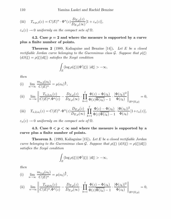
(iii) Tn,p,β(z) = C(E)n · Φn(z)DE,ρ(z)
DE,ρ(∞)[1 + εn(z)],
εn(z) → 0 uniformly on the compact sets of Ω.
4.2. Case p = 2 and where the measure is supported by a curveplus a finite number of points.
Theorem 2 (1989, Kaliaguine and Benzine [14]). Let E be a closedrectifiable Jordan curve belonging to the Gueronimus class G. Suppose that ρ(ξ)(dβ(ξ) = ρ(ξ)|dξ|) satisfies the Szego condition
∫
E(log ρ(ξ))|Φ′(ξ)| |dξ| > −∞,
then
(i) limn→∞
mn,2(α`)
C(E)n= µ(α`)
1
2 ,
(ii) limn→∞
∥∥∥∥∥Tn,2,αl
(z)
C(E)n.Φn(z)− DE,ρ(z)
DE,ρ(∞)·∏
k=1
Φ(z) − Φ(zk)
Φ(z)Φ(zk) − 1· |Φ(zk)|2
Φ(zk)
∥∥∥∥∥Hp(Ω,ρ)
= 0,
(iii) Tn,2,αl(z) = C(E)n ·Φn(z)
DE,ρ(z)
DE,ρ(∞)·∏
k=1
Φ(z) − Φ(zk)
Φ(z)Φ(zk) − 1· |Φ(zk)|2
Φ(zk)[1+εn(z)],
εn(z) → 0 uniformly on the compact sets of Ω.
4.3. Case 0 < p < ∞ and where the measure is supported by acurve plus a finite number of points.
Theorem 3. (1993, Kaliaguine [15]). Let E be a closed rectifiable Jordancurve belonging to the Gueronimus class G. Suppose that ρ(ξ) (dβ(ξ) = ρ(ξ)|dξ|)satisfies the Szego condition
∫
E(log ρ(ξ))|Φ′(ξ)| |dξ| > −∞,
then
(i) limn→∞
mn,p(α`)
C(E)n= µ(α`)
1
p ,
(ii) limn→∞
∥∥∥∥∥Tn,p,αl
(z)
C(E)n.Φn(z)− DE,ρ(z)
DE,ρ(∞)·∏
k=1
Φ(z) − Φ(zk)
Φ(z)Φ(zk) − 1· |Φ(zk)|2
Φ(zk)
∥∥∥∥∥Hp(Ω,ρ)
= 0,
Lp extremal polynomials 111
(iii) Tn,p,αl(z) = C(E)n ·Φn(z)
DE,ρ(z)
DE,ρ(∞)·∏
k=1
Φ(z) − Φ(zk)
Φ(z)Φ(zk) − 1· |Φ(zk)|2
Φ(zk)[1+εn(z)],
εn(z) → 0 uniformly on the compact sets of Ω.
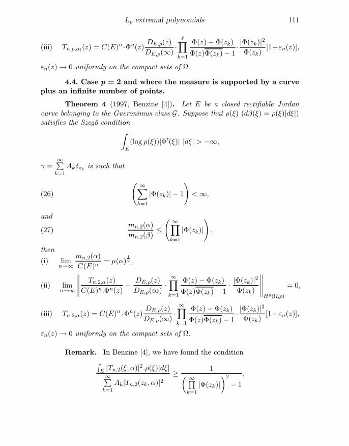
4.4. Case p = 2 and where the measure is supported by a curveplus an infinite number of points.
Theorem 4 (1997, Benzine [4]). Let E be a closed rectifiable Jordancurve belonging to the Gueronimus class G. Suppose that ρ(ξ) (dβ(ξ) = ρ(ξ)|dξ|)satisfies the Szego condition
∫
E(log ρ(ξ))|Φ′(ξ)| |dξ| > −∞,
γ =∞∑
k=1
Akδzkis such that
(∞∑
k=1
|Φ(zk)| − 1
)<∞,(26)
andmn,2(α)
mn,2(β)≤(
∞∏
k=1
|Φ(zk)|),(27)
then
(i) limn→∞
mn,2(α)
C(E)n= µ(α)
1
2 ,
(ii) limn→∞
∥∥∥∥∥Tn,2,α(z)
C(E)n.Φn(z)− DE,ρ(z)
DE,ρ(∞)·
∞∏
k=1
Φ(z) − Φ(zk)
Φ(z)Φ(zk) − 1· |Φ(zk)|2
Φ(zk)
∥∥∥∥∥Hp(Ω,ρ)
= 0,
(iii) Tn,2,α(z) = C(E)n ·Φn(z)DE,ρ(z)
DE,ρ(∞)·∞∏
k=1
Φ(z) − Φ(zk)
Φ(z)Φ(zk) − 1· |Φ(zk)|2
Φ(zk)[1+εn(z)],
εn(z) → 0 uniformly on the compact sets of Ω.
Remark. In Benzine [4], we have found the condition
∫E |Tn,2(ξ, α)|2.ρ(ξ)|dξ|∞∑
k=1
Ak|Tn,2(zk, α)|2≥ 1(
∞∏k=1
|Φ(zk)|)2
− 1
,
112 Yamina Laskri and Rachid Benzine
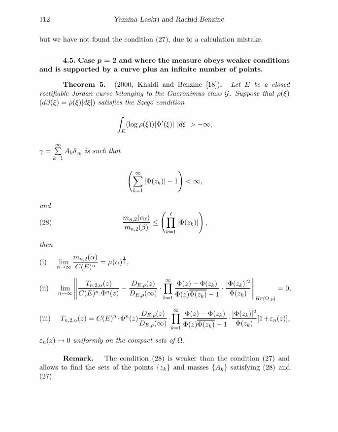
but we have not found the condition (27), due to a calculation mistake.
4.5. Case p = 2 and where the measure obeys weaker conditionsand is supported by a curve plus an infinite number of points.
Theorem 5. (2000, Khaldi and Benzine [18]). Let E be a closedrectifiable Jordan curve belonging to the Gueronimus class G. Suppose that ρ(ξ)(dβ(ξ) = ρ(ξ)|dξ|) satisfies the Szego condition
∫
E(log ρ(ξ))|Φ′(ξ)| |dξ| > −∞,
γ =∞∑
k=1
Akδzkis such that
(∞∑
k=1
|Φ(zk)| − 1
)<∞,
and
mn,2(α`)
mn,2(β)≤(∏
k=1
|Φ(zk)|),(28)
then
(i) limn→∞
mn,2(α)
C(E)n= µ(α)
1
2 ,
(ii) limn→∞
∥∥∥∥∥Tn,2,α(z)
C(E)n.Φn(z)− DE,ρ(z)
DE,ρ(∞)·
∞∏
k=1
Φ(z) − Φ(zk)
Φ(z)Φ(zk) − 1· |Φ(zk)|2
Φ(zk)
∥∥∥∥∥Hp(Ω,ρ)
= 0,
(iii) Tn,2,α(z) = C(E)n ·Φn(z)DE,ρ(z)
DE,ρ(∞)·∞∏
k=1
Φ(z) − Φ(zk)
Φ(z)Φ(zk) − 1· |Φ(zk)|2
Φ(zk)[1+εn(z)],
εn(z) → 0 uniformly on the compact sets of Ω.
Remark. The condition (28) is weaker than the condition (27) andallows to find the sets of the points zk and masses Ak satisfying (28) and(27).
Lp extremal polynomials 113
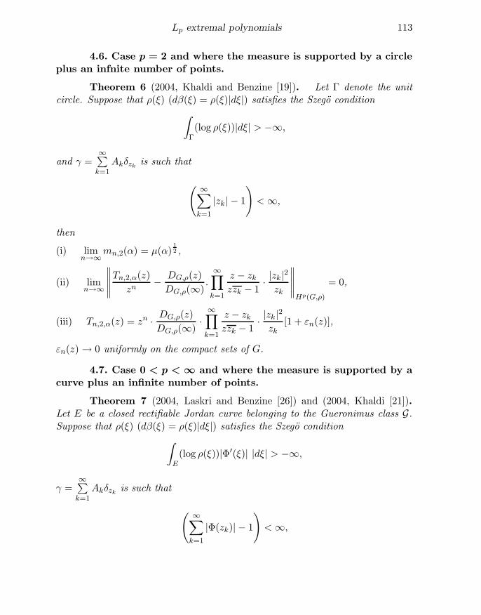
4.6. Case p = 2 and where the measure is supported by a circleplus an infnite number of points.
Theorem 6 (2004, Khaldi and Benzine [19]). Let Γ denote the unitcircle. Suppose that ρ(ξ) (dβ(ξ) = ρ(ξ)|dξ|) satisfies the Szego condition
∫
Γ(log ρ(ξ))|dξ| > −∞,
and γ =∞∑
k=1
Akδzkis such that
(∞∑
k=1
|zk| − 1
)<∞,
then
(i) limn→∞
mn,2(α) = µ(α)1
2 ,
(ii) limn→∞
∥∥∥∥∥Tn,2,α(z)
zn− DG,ρ(z)
DG,ρ(∞).
∞∏
k=1
z − zkzzk − 1
· |zk|2
zk
∥∥∥∥∥Hp(G,ρ)
= 0,
(iii) Tn,2,α(z) = zn · DG,ρ(z)
DG,ρ(∞)·
∞∏
k=1
z − zkzzk − 1
· |zk|2
zk[1 + εn(z)],
εn(z) → 0 uniformly on the compact sets of G.
4.7. Case 0 < p < ∞ and where the measure is supported by acurve plus an infinite number of points.
Theorem 7 (2004, Laskri and Benzine [26]) and (2004, Khaldi [21]).Let E be a closed rectifiable Jordan curve belonging to the Gueronimus class G.Suppose that ρ(ξ) (dβ(ξ) = ρ(ξ)|dξ|) satisfies the Szego condition
∫
E(log ρ(ξ))|Φ′(ξ)| |dξ| > −∞,
γ =∞∑
k=1
Akδzkis such that
(∞∑
k=1
|Φ(zk)| − 1
)<∞,
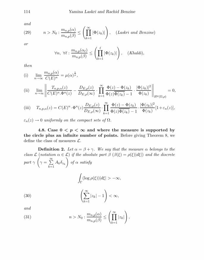
114 Yamina Laskri and Rachid Benzine
and
n > N0 :mn,p(α)
mn,p(β)≤(
∞∏
k=1
|Φ(zk)|), (Laskri and Benzine)(29)
or
∀n, ∀` :mn,p(α`)
mn,p(β)≤(∏
k=1
|Φ(zk)|), (Khaldi),
then
(i) limn→∞
mn,p(α)
C(E)n= µ(α)
1
p ,
(ii) limn→∞
∥∥∥∥∥Tn,p,α(z)
C(E)n.Φn(z)− DE,ρ(z)
DE,ρ(∞)·
∞∏
k=1
Φ(z) − Φ(zk)
Φ(z)Φ(zk) − 1· |Φ(zk)|2
Φ(zk)
∥∥∥∥∥Hp(Ω,ρ)
= 0,
(iii) Tn,p,α(z) = C(E)n ·Φn(z)DE,ρ(z)
DE,ρ(∞)·∞∏
k=1
Φ(z) − Φ(zk)
Φ(z)Φ(zk) − 1· |Φ(zk)|2
Φ(zk)[1+εn(z)],
εn(z) → 0 uniformly on the compact sets of Ω.
4.8. Case 0 < p < ∞ and where the measure is supported bythe circle plus an infinite number of points. Before giving Theorem 8, wedefine the class of measures L.
Definition 2. Let α = β + γ. We say that the measure α belongs to theclass L (notation α ∈ L) if the absolute part β (β(ξ) = ρ(ξ)|dξ|) and the discrete
part γ
(γ =
∞∑k=1
Akδzk
)of α satisfy
∫
Γ(log ρ(ξ))|dξ| > −∞,
(∞∑
k=1
|zk| − 1
)<∞,(30)
and
n > N0 :mn,p(α)
mn,p(β)≤(
∞∏
k=1
|zk|),(31)
Lp extremal polynomials 115
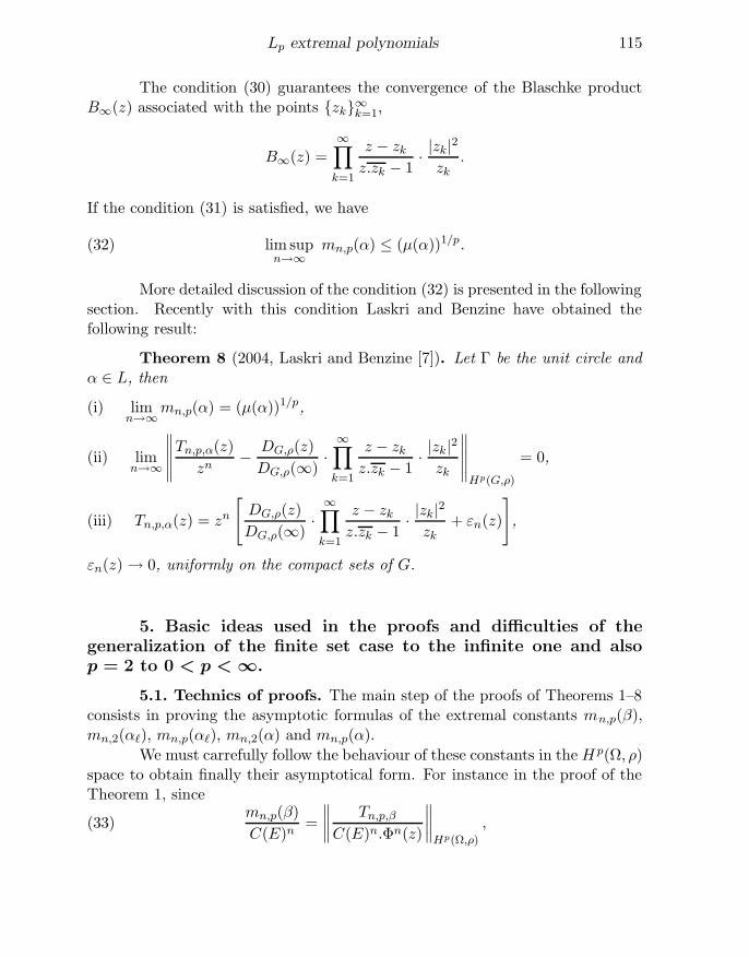
The condition (30) guarantees the convergence of the Blaschke productB∞(z) associated with the points zk∞k=1,
B∞(z) =∞∏
k=1
z − zkz.zk − 1
· |zk|2
zk.
If the condition (31) is satisfied, we have
lim supn→∞
mn,p(α) ≤ (µ(α))1/p.(32)
More detailed discussion of the condition (32) is presented in the followingsection. Recently with this condition Laskri and Benzine have obtained thefollowing result:
Theorem 8 (2004, Laskri and Benzine [7]). Let Γ be the unit circle andα ∈ L, then
(i) limn→∞
mn,p(α) = (µ(α))1/p,
(ii) limn→∞
∥∥∥∥∥Tn,p,α(z)
zn− DG,ρ(z)
DG,ρ(∞)·
∞∏
k=1
z − zkz.zk − 1
· |zk|2
zk
∥∥∥∥∥Hp(G,ρ)
= 0,
(iii) Tn,p,α(z) = zn
[DG,ρ(z)
DG,ρ(∞)·
∞∏
k=1
z − zkz.zk − 1
· |zk|2
zk+ εn(z)
],
εn(z) → 0, uniformly on the compact sets of G.
5. Basic ideas used in the proofs and difficulties of the
generalization of the finite set case to the infinite one and also
p = 2 to 0 < p < ∞.
5.1. Technics of proofs. The main step of the proofs of Theorems 1–8consists in proving the asymptotic formulas of the extremal constants mn,p(β),mn,2(α`), mn,p(α`), mn,2(α) and mn,p(α).
We must carrefully follow the behaviour of these constants in the H p(Ω, ρ)space to obtain finally their asymptotical form. For instance in the proof of theTheorem 1, since
mn,p(β)
C(E)n=
∥∥∥∥Tn,p,β
C(E)n.Φn(z)
∥∥∥∥Hp(Ω,ρ)
,(33)
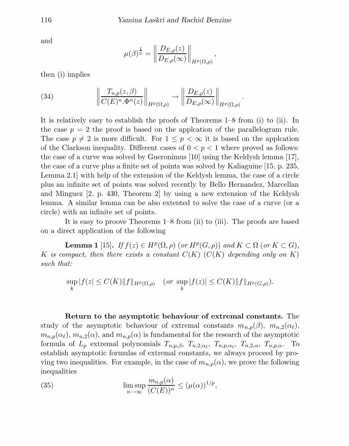
116 Yamina Laskri and Rachid Benzine
and
µ(β)1
p =
∥∥∥∥DE,ρ(z)
DE,ρ(∞)
∥∥∥∥Hp(Ω,ρ)
,
then (i) implies
∥∥∥∥Tn,p(z, β)
C(E)n.Φn(z)
∥∥∥∥Hp(Ω,ρ)
→∥∥∥∥DE,ρ(z)
DE,ρ(∞)
∥∥∥∥Hp(Ω,ρ)
.(34)
It is relatively easy to establish the proofs of Theorems 1–8 from (i) to (ii). Inthe case p = 2 the proof is based on the applcation of the parallelogram rule.The case p 6= 2 is more difficult. For 1 ≤ p < ∞ it is based on the applcationof the Clarkson inequality. Different cases of 0 < p < 1 where proved as follows:the case of a curve was solved by Gueronimus [10] using the Keldysh lemma [17],the case of a curve plus a finite set of points was solved by Kaliaguine [15, p. 235,Lemma 2.1] with help of the extension of the Keldysh lemma, the case of a circleplus an infinite set of points was solved recently by Bello Hernandez, Marcellanand Minguez [2, p. 430, Theorem 2] by using a new extension of the Keldyshlemma. A similar lemma can be also extented to solve the case of a curve (or acircle) with an infinite set of points.
It is easy to proove Theorems 1–8 from (ii) to (iii). The proofs are basedon a direct application of the following
Lemma 1 [15]. If f(z) ∈ Hp(Ω, ρ) (or Hp(G, ρ)) and K ⊂ Ω (or K ⊂ G),K is compact, then there exists a constant C(K) (C(K) depending only on K)such that:
supk
|f(z| ≤ C(K)‖f‖Hp(Ω,ρ) (or supk
|f(z)| ≤ C(K)‖f‖Hp(G,ρ)).
Return to the asymptotic behaviour of extremal constants. Thestudy of the asymptotic behaviour of extremal constants mn,p(β), mn,2(α`),mn,p(α`), mn,2(α), and mn,p(α) is fundamental for the research of the asymptoticformula of Lp extremal polynomials Tn,p,β, Tn,2,α`
, Tn,p,α`, Tn,2,α, Tn,p,α. To
establish asymptotic formulas of extremal constants, we always proceed by pro-ving two inequalities. For example, in the case of mn,p(α), we prove the followinginequalities
lim supn→∞
mn,p(α)
(C(E))n≤ (µ(α))1/p,(35)
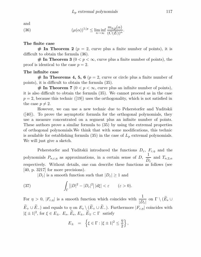
Lp extremal polynomials 117
and
(µ(α))1/p ≤ lim infn→∞
mn,p(α)
(C(E))n.(36)
The finite case# In Theorem 2 (p = 2, curve plus a finite number of points), it is
difficult to obtain the formula (36).# In Theorem 3 (0 < p <∞, curve plus a finite number of points), the
proof is identical to the case p = 2.
The infinite case# In Theorems 4, 5, 6 (p = 2, curve or circle plus a finite number of
points), it is difficult to obtain the formula (35).# In Theorem 7 (0 < p <∞, curve plus an infinite number of points),
it is also difficult to obtain the formula (35). We cannot proceed as in the casep = 2, because this technic ([19]) uses the orthogonality, which is not satisfied inthe case p 6= 2.
However, we can use a new technic due to Peherstorfer and Yuditskii([40]). To prove the asymptotic formula for the orthogonal polynomials, theyuse a measure concentrated on a segment plus an infinite number of points.These authors prove a similar formula to (35) by using the extremal propertiesof orthogonal polynomials.We think that with some modifications, this technicis available for establishing formula (35) in the case of Lp extremal polynomials.We will just give a sketch.
Peherstorfer and Yuditskii introduced the functions Dε, Fε,η and the
polynomials Pn,ε,η as approximations, in a certain sense of D,1
Dεand Tn,2,α
respectively. Without details, one can describe these functions as follows (see[40, p. 3217] for more precisions).
|Dε| is a smooth function such that |Dε| ≥ 1 and∫
Γ
∣∣|D|2 − |Dε|2∣∣ |dξ| < ε (ε > 0).(37)
For η > 0, |Fε,η| is a smooth function which coincides with1
|Dε|on Γ \ (Es ∪
E+ ∪ E−) and equals to η on Es \ (E+ ∪ E−). Furthermore |Fε,η| coincides with
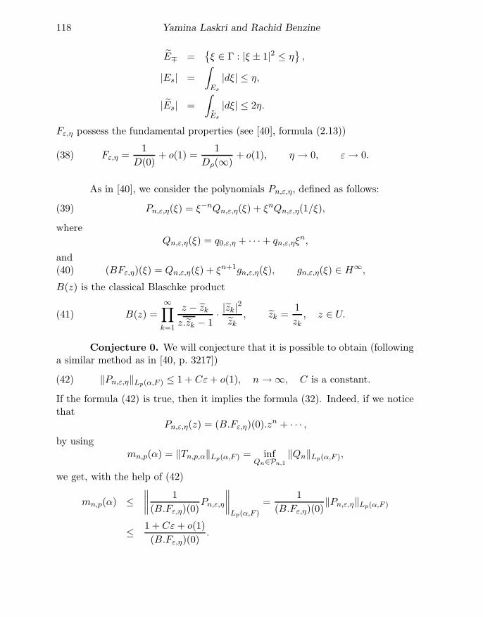
|ξ ± 1|2, for ξ ∈ E±. Es, Es, E±, E∓ ⊂ Γ satisfy
E± =ξ ∈ Γ : |ξ ± 1|2 ≤ η
2
,
118 Yamina Laskri and Rachid Benzine
E∓ =ξ ∈ Γ : |ξ ± 1|2 ≤ η
,
|Es| =
∫
Es
|dξ| ≤ η,
|Es| =
∫
Es
|dξ| ≤ 2η.
Fε,η possess the fundamental properties (see [40], formula (2.13))
Fε,η =1
D(0)+ o(1) =
1
Dρ(∞)+ o(1), η → 0, ε→ 0.(38)
As in [40], we consider the polynomials Pn,ε,η, defined as follows:
Pn,ε,η(ξ) = ξ−nQn,ε,η(ξ) + ξnQn,ε,η(1/ξ),(39)
whereQn,ε,η(ξ) = q0,ε,η + · · · + qn,ε,ηξ
n,
and(BFε,η)(ξ) = Qn,ε,η(ξ) + ξn+1gn,ε,η(ξ), gn,ε,η(ξ) ∈ H∞,(40)
B(z) is the classical Blaschke product
B(z) =
∞∏
k=1
z − zk
z.zk − 1· |zk|
2
zk, zk =
1
zk, z ∈ U.(41)
Conjecture 0. We will conjecture that it is possible to obtain (followinga similar method as in [40, p. 3217])
‖Pn,ε,η‖Lp(α,F ) ≤ 1 + Cε+ o(1), n→ ∞, C is a constant.(42)
If the formula (42) is true, then it implies the formula (32). Indeed, if we noticethat
Pn,ε,η(z) = (B.Fε,η)(0).zn + · · · ,
by usingmn,p(α) = ‖Tn,p,α‖Lp(α,F ) = inf
Qn∈Pn,1
‖Qn‖Lp(α,F ),
we get, with the help of (42)
mn,p(α) ≤∥∥∥∥
1
(B.Fε,η)(0)Pn,ε,η
∥∥∥∥Lp(α,F )
=1
(B.Fε,η)(0)‖Pn,ε,η‖Lp(α,F )
≤ 1 + Cε+ o(1)
(B.Fε,η)(0).
Lp extremal polynomials 119
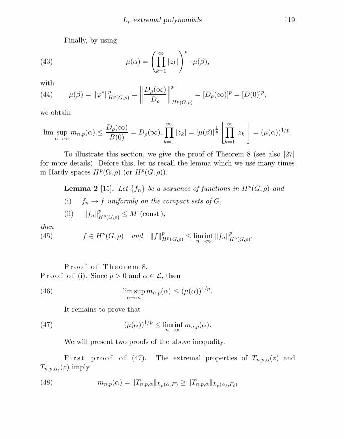
Finally, by using
µ(α) =
(∞∏
k=1
|zk|)p
· µ(β),(43)
with
µ(β) = ‖ϕ∗‖pHp(G,ρ) =
∥∥∥∥Dρ(∞)
Dρ
∥∥∥∥p
Hp(G,ρ)
= [Dρ(∞)]p = [D(0)]p,(44)
we obtain
lim supn→∞
mn,p(α) ≤ Dρ(∞)
B(0)= Dρ(∞).
∞∏
k=1
|zk| = [µ(β)]1
p
[∞∏
k=1
|zk|]
= (µ(α))1/p.
To illustrate this section, we give the proof of Theorem 8 (see also [27]for more details). Before this, let us recall the lemma which we use many timesin Hardy spaces Hp(Ω, ρ) (or Hp(G, ρ)).
Lemma 2 [15]. Let fn be a sequence of functions in Hp(G, ρ) and
(i) fn → f uniformly on the compact sets of G,
(ii) ‖fn‖pHp(G,ρ) ≤M (const ),
thenf ∈ Hp(G, ρ) and ‖f‖p
Hp(G,ρ) ≤ lim infn→∞
‖fn‖pHp(G,ρ).(45)
P r o o f o f Th e o r em 8.P r o o f o f (i). Since p > 0 and α ∈ L, then
lim supn→∞
mn,p(α) ≤ (µ(α))1/p.(46)
It remains to prove that
(µ(α))1/p ≤ lim infn→∞
mn,p(α).(47)
We will present two proofs of the above inequality.
F i r s t p r o o f o f (47). The extremal properties of Tn,p,α(z) andTn,p,α`
(z) imply
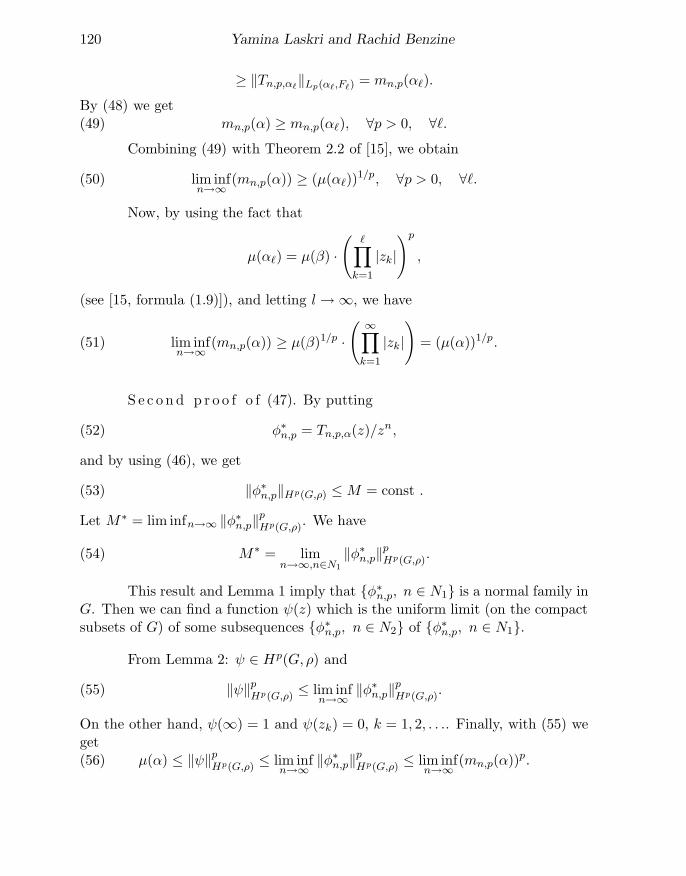
mn,p(α) = ‖Tn,p,α‖Lp(α,F ) ≥ ‖Tn,p,α‖Lp(α`,F`)(48)
120 Yamina Laskri and Rachid Benzine
≥ ‖Tn,p,α`‖Lp(α`,F`) = mn,p(α`).
By (48) we getmn,p(α) ≥ mn,p(α`), ∀p > 0, ∀`.(49)
Combining (49) with Theorem 2.2 of [15], we obtain
lim infn→∞
(mn,p(α)) ≥ (µ(α`))1/p, ∀p > 0, ∀`.(50)
Now, by using the fact that
µ(α`) = µ(β) ·(∏
k=1
|zk|)p
,
(see [15, formula (1.9)]), and letting l → ∞, we have
lim infn→∞
(mn,p(α)) ≥ µ(β)1/p ·(
∞∏
k=1
|zk|)
= (µ(α))1/p.(51)
S e c o n d p r o o f o f (47). By putting
φ∗n,p = Tn,p,α(z)/zn,(52)
and by using (46), we get
‖φ∗n,p‖Hp(G,ρ) ≤M = const .(53)
Let M∗ = lim infn→∞ ‖φ∗n,p‖pHp(G,ρ). We have
M∗ = limn→∞,n∈N1
‖φ∗n,p‖pHp(G,ρ).(54)
This result and Lemma 1 imply that φ∗n,p, n ∈ N1 is a normal family in
G. Then we can find a function ψ(z) which is the uniform limit (on the compactsubsets of G) of some subsequences φ∗
n,p, n ∈ N2 of φ∗n,p, n ∈ N1.
From Lemma 2: ψ ∈ Hp(G, ρ) and
‖ψ‖pHp(G,ρ) ≤ lim inf
n→∞‖φ∗n,p‖p
Hp(G,ρ).(55)
On the other hand, ψ(∞) = 1 and ψ(zk) = 0, k = 1, 2, . . .. Finally, with (55) weget
µ(α) ≤ ‖ψ‖pHp(G,ρ) ≤ lim inf
n→∞‖φ∗n,p‖p
Hp(G,ρ) ≤ lim infn→∞
(mn,p(α))p.(56)
Lp extremal polynomials 121
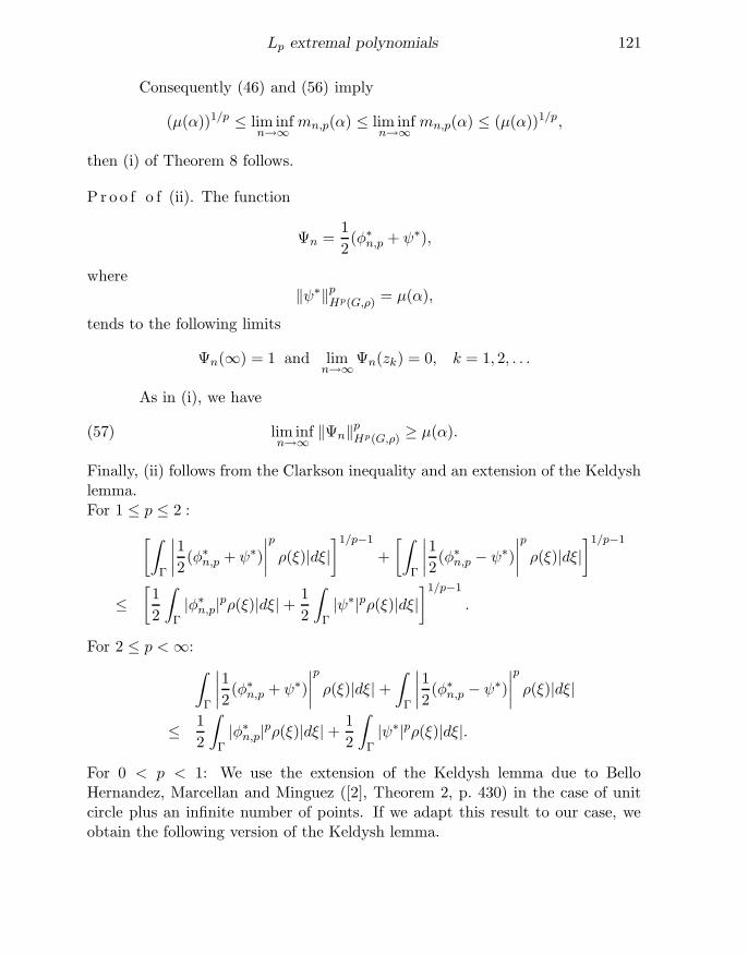
Consequently (46) and (56) imply
(µ(α))1/p ≤ lim infn→∞
mn,p(α) ≤ lim infn→∞
mn,p(α) ≤ (µ(α))1/p,
then (i) of Theorem 8 follows.
P r o o f o f (ii). The function
Ψn =1
2(φ∗n,p + ψ∗),
where‖ψ∗‖p
Hp(G,ρ) = µ(α),
tends to the following limits
Ψn(∞) = 1 and limn→∞
Ψn(zk) = 0, k = 1, 2, . . .
As in (i), we have
lim infn→∞
‖Ψn‖pHp(G,ρ) ≥ µ(α).(57)
Finally, (ii) follows from the Clarkson inequality and an extension of the Keldyshlemma.For 1 ≤ p ≤ 2 :
[∫
Γ
∣∣∣∣1
2(φ∗n,p + ψ∗)
∣∣∣∣p
ρ(ξ)|dξ|]1/p−1
+
[∫
Γ
∣∣∣∣1
2(φ∗n,p − ψ∗)
∣∣∣∣p
ρ(ξ)|dξ|]1/p−1
≤[1
2
∫
Γ|φ∗n,p|pρ(ξ)|dξ| +
1
2
∫
Γ|ψ∗|pρ(ξ)|dξ|
]1/p−1
.
For 2 ≤ p <∞:
∫
Γ
∣∣∣∣1
2(φ∗n,p + ψ∗)
∣∣∣∣p
ρ(ξ)|dξ| +∫
Γ
∣∣∣∣1
2(φ∗n,p − ψ∗)
∣∣∣∣p
ρ(ξ)|dξ|
≤ 1
2
∫
Γ|φ∗n,p|pρ(ξ)|dξ| +
1
2
∫
Γ|ψ∗|pρ(ξ)|dξ|.
For 0 < p < 1: We use the extension of the Keldysh lemma due to BelloHernandez, Marcellan and Minguez ([2], Theorem 2, p. 430) in the case of unitcircle plus an infinite number of points. If we adapt this result to our case, weobtain the following version of the Keldysh lemma.
122 Yamina Laskri and Rachid Benzine
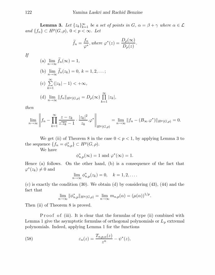
Lemma 3. Let zk∞k=1 be a set of points in G, α = β + γ where α ∈ Land fn ⊂ Hp(G, ρ), 0 < p <∞. Let
fn =fn
ϕ∗,where ϕ∗(z) =
Dρ(∞)
Dρ(z).
If(a) lim
n→∞fn(∞) = 1,
(b) limn→∞
fn(zk) = 0, k = 1, 2, . . . ;
(c)∞∑
k=1
(|zk| − 1) < +∞,
(d) limn→∞
‖fn‖Hp(G,ρ) = Dρ(∞)∞∏
k=1
|zk|,
then
limn→∞
∥∥∥∥∥fn −∞∏
k=1
z − zkz.zk − 1
· |zk|2
zk.ϕ∗
∥∥∥∥∥Hp(G,ρ)
= limn→∞
‖fn − (B∞.ϕ∗)‖Hp(G,ρ) = 0.
We get (ii) of Theorem 8 in the case 0 < p < 1, by applying Lemma 3 tothe sequence fn = φ∗n,p ⊂ Hp(G, ρ).
We haveφ∗n,p(∞) = 1 and ϕ∗(∞) = 1.
Hence (a) follows. On the other hand, (b) is a consequence of the fact thatϕ∗(zk) 6= 0 and
limn→∞
φ∗n,p(zk) = 0, k = 1, 2, . . . .
(c) is exactly the condition (30). We obtain (d) by considering (43), (44) and thefact that
limn→∞
‖φ∗n,p‖Hp(G,ρ) = limn→∞
mn,p(α) = (µ(α))1/p.
Then (ii) of Theorem 8 is proved.
P r o o f o f (iii). It is clear that the formulas of type (ii) combined withLemma 1 give the asymptotic formulas of orthogonal polynomials or Lp extremalpolynomials. Indeed, applying Lemma 1 for the functions
εn(z) =Tn,p,α(z)
zn− ψ∗(z),(58)
Lp extremal polynomials 123
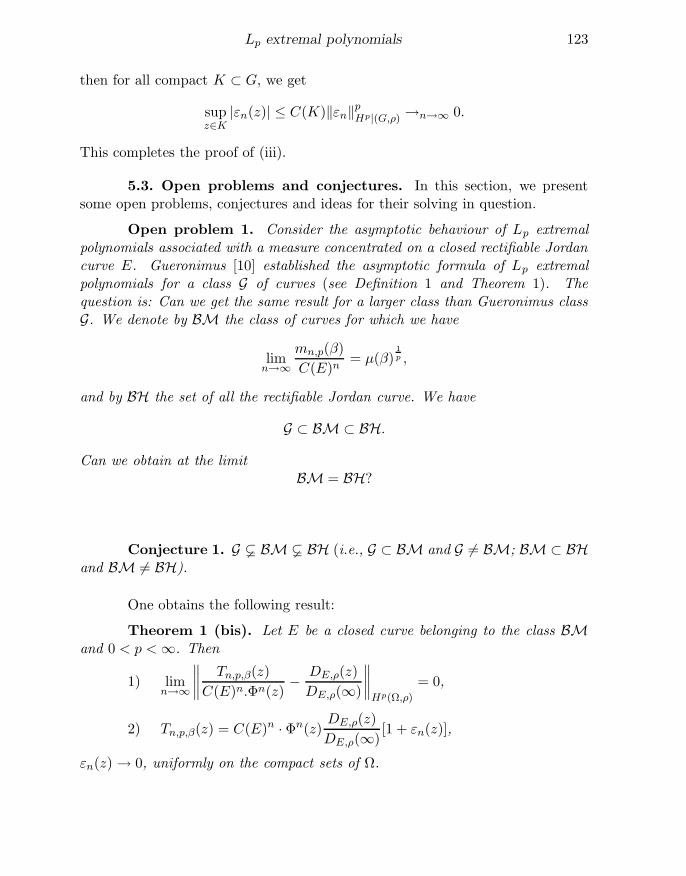
then for all compact K ⊂ G, we get
supz∈K
|εn(z)| ≤ C(K)‖εn‖pHp|(G,ρ) →n→∞ 0.
This completes the proof of (iii).
5.3. Open problems and conjectures. In this section, we presentsome open problems, conjectures and ideas for their solving in question.
Open problem 1. Consider the asymptotic behaviour of Lp extremalpolynomials associated with a measure concentrated on a closed rectifiable Jordancurve E. Gueronimus [10] established the asymptotic formula of Lp extremalpolynomials for a class G of curves (see Definition 1 and Theorem 1). Thequestion is: Can we get the same result for a larger class than Gueronimus classG. We denote by BM the class of curves for which we have
limn→∞
mn,p(β)
C(E)n= µ(β)
1
p ,
and by BH the set of all the rectifiable Jordan curve. We have
G ⊂ BM ⊂ BH.
Can we obtain at the limitBM = BH?
Conjecture 1. G BM BH (i.e., G ⊂ BM and G 6= BM; BM ⊂ BHand BM 6= BH).
One obtains the following result:
Theorem 1 (bis). Let E be a closed curve belonging to the class BMand 0 < p <∞. Then
1) limn→∞
∥∥∥∥Tn,p,β(z)
C(E)n.Φn(z)− DE,ρ(z)
DE,ρ(∞)
∥∥∥∥Hp(Ω,ρ)
= 0,
2) Tn,p,β(z) = C(E)n · Φn(z)DE,ρ(z)
DE,ρ(∞)[1 + εn(z)],
εn(z) → 0, uniformly on the compact sets of Ω.
124 Yamina Laskri and Rachid Benzine
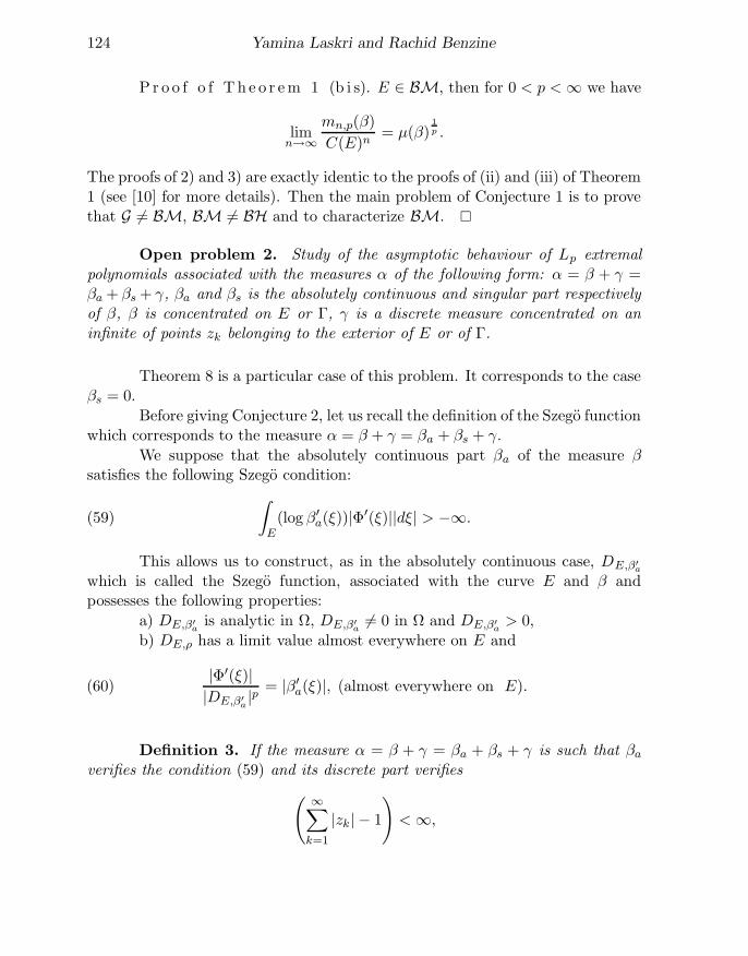
P r o o f o f Th e o r e m 1 (b i s). E ∈ BM, then for 0 < p <∞ we have
limn→∞
mn,p(β)
C(E)n= µ(β)
1
p .
The proofs of 2) and 3) are exactly identic to the proofs of (ii) and (iii) of Theorem1 (see [10] for more details). Then the main problem of Conjecture 1 is to provethat G 6= BM, BM 6= BH and to characterize BM.
Open problem 2. Study of the asymptotic behaviour of Lp extremalpolynomials associated with the measures α of the following form: α = β + γ =βa + βs + γ, βa and βs is the absolutely continuous and singular part respectivelyof β, β is concentrated on E or Γ, γ is a discrete measure concentrated on aninfinite of points zk belonging to the exterior of E or of Γ.
Theorem 8 is a particular case of this problem. It corresponds to the caseβs = 0.
Before giving Conjecture 2, let us recall the definition of the Szego functionwhich corresponds to the measure α = β + γ = βa + βs + γ.
We suppose that the absolutely continuous part βa of the measure βsatisfies the following Szego condition:
∫
E(log β′
a(ξ))|Φ′(ξ)||dξ| > −∞.(59)
This allows us to construct, as in the absolutely continuous case, DE,β′
a
which is called the Szego function, associated with the curve E and β andpossesses the following properties:
a) DE,β′
ais analytic in Ω, DE,β′
a6= 0 in Ω and DE,β′
a> 0,
b) DE,ρ has a limit value almost everywhere on E and
|Φ′(ξ)||DE,β′
a|p = |β′a(ξ)|, (almost everywhere on E).(60)
Definition 3. If the measure α = β + γ = βa + βs + γ is such that βa
verifies the condition (59) and its discrete part verifies
(∞∑
k=1
|zk| − 1
)<∞,
Lp extremal polynomials 125
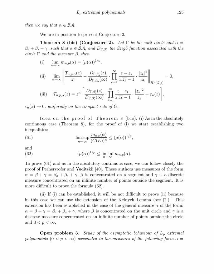
then we say that α ∈ BA.
We are in position to present Conjecture 2.
Theorem 8 (bis) (Conjecture 2). Let Γ be the unit circle and α =βa + βs + γ, such that α ∈ BA, and DΓ,β′
athe Szego function associated with the
circle Γ and the measure β, then
(i) limn→∞
mn,p(α) = (µ(α))1/p,
(ii) limn→∞
∥∥∥∥∥Tn,p,α(z)
zn− DΓ,β′
a(z)
DΓ,β′
a(∞)
·∞∏
k=1
z − zkz.zk − 1
· |zk|2
zk
∥∥∥∥∥Hp(G,ρ)
= 0,
(iii) Tn,p,α(z) = zn
[DΓ,β′
a(z)
DΓ,β′
a(∞)
·∞∏
k=1
z − zkz.zk − 1
· |zk|2
zk+ εn(z)
],
εn(z) → 0, uniformly on the compact sets of G.
I d e a o n t h e p r o o f o f Th e o r e m 8 (b i s). (i) As in the absolutelycontinuous case (Theorem 8), for the proof of (i) we start establishing twoinequalities:
lim supn→∞
mn,p(α)
(C(E))n≤ (µ(α))1/p,(61)
and
(µ(α))1/p ≤ lim infn→∞
mn,p(α).(62)
To prove (61) and as in the absolutely continuous case, we can follow closely theproof of Perherstofer and Yuditskii [40]. These authors use measures of the formα = β + γ = βa + βs + γ, β is concentrated on a segment and γ is a discretemeasure concentrated on an infinite number of points outside the segment. It ismore difficult to prove the formula (62).
(ii) If (i) can be established, it will be not difficult to prove (ii) becausein this case we can use the extension of the Keldych Lemma (see [2]). Thisextension has been established in the case of the general measure α of the form:α = β + γ = βa + βs + γ, where β is concentrated on the unit circle and γ is adiscrete measure concentrated on an infinite number of points outside the circleand 0 < p <∞.
Open problem 3. Study of the asymptotic behaviour of Lp extremalpolynomials (0 < p < ∞) associated to the measures of the following form α =
126 Yamina Laskri and Rachid Benzine
β+γ, where β is concentrated on the arc (segment), and is absolutely continuousor not, and γ is a discrete measure concentrated on an infinite number of pointszk∞k=1.
This is a difficult problem. It has been only solved for the particular casep = 2 for a finite number of points and an absolutely continuous measure byKaliaguine [16].
REFERE NCES
[1] A. Adamov. Uber asymptotische Ausdrucke fur die Polynome Un(x) =
e1
2ax2 dn
dxn (e−1
2ax2
) fur sehr große Werte von n. St. Petersb. Polyt. Inst. 5(1907) 127–143 (in Russian).
[2] M. Bello Hernandez, F. Marcellan, J. Minguez Ceniceros. Pseudouniform convexity in Hp and some extremal problems on Sobolev spaces.Complex variables, Theory Appl. 48, 5 (2003) 429–440.
[3] M. Bello Hernandez, J. Minguez Ceniceros. Strong asymptoticbehaviour for extremal polynomials with respect to varying measures onthe unit circle. J. Approx. Theory 125, 1 (2003) 131–144.
[4] R Benzine. Asymptotic behaviour of orthogonal polynomials correspondingto a measure with infinite discrete part off a curve. J. Approx. Theory 89(1997) 257–265.
[5] S. N. Bernstein. Sur les polynomes orthogonaux relatifs a un segment finiI, II. J. Math. Pures Appl. 9 (1930) 127–177; 10 (1931) 219–286.
[6] G. Darboux. Memoire sur l’approximation des fonctions de tres grandsnombres, et sur une classe etendue de developpements en serie. Liouville J.(3) IV (1878), 5–56, 377–416.
[7] P. L. Duren. Theory of Hp Spaces. Academic Press, New York, 1970.
[8] L. Fejer. Uber die Bestimmung asymptotischer Werte. Math. es termesz.ert. 27 (1909) 1–33 (in Hungarian).
[9] J.S. Geronimo, K. M. Case. Scattering theory and polynomialsorthogonal on the real line. Trans. Amer. Math. Soc. 258 (1980), 467–494,MR 82:c:81138.
Lp extremal polynomials 127
[10] Ya. L. Gueronimus. On some extremal problems in the space Lpσ. Mat.
Sb. (N.S.) 31(73) (1952), 3–26 (in Russian).
[11] Ya. L. Gueronimus. Polynomials Orthogonal on a Circle and Interval.Fizmatgiz, Moscow, 1958 (in Russian); (English translation: InternationalSeries of Monographs on Pure and Applied Mathematics, 18, Oxford-London-New York-Paris: Pergamon Press, 1961, 218 p.).
[12] A. A. Gonchar. On convergence of Pade approximants for some classes ofmeromorphic functions. Mat. Sb. 97(139), 4 (1975).
[13] E. Heine. Handbuch der Kugelfunctionen, Theorie und Anwendungen. Vols.I, II. 2nd edition. Berlin, 1878, 1881.
[14] V. Kaliaguine, R. Benzine. Sur la formule asymptotique des polynomesorthogonaux associes a une mesure concentree sur un contour plus une partiediscrete finie. Bull. Soc. Math. Belg. Ser. B 41, 1 (1989) 29–46.
[15] V. Kaliaguine. On Asymptotics of Lp extremal polynomials on a complexcurve (0 < p <∞). J. Approx. Theory 74 (1993), 226–236.
[16] V. Kaliaguine. A note on the asymptotics of orthogonal polynomials on acomplex arc: The case of a measure with a discrete part. J. Approx. Theory80 (1995), 138–145.
[17] M. V. Keldysh. Selected works. Moskva, Nauka, 1985, 448 p. (in Russian).
[18] R. Khaldi, R. Benzine. On a generalization of an asymptotic formula oforthogonal polynomials. Int. J. Appl. Math. 4, 3 (2000), 261–274.
[19] R. Khaldi, R. Benzine. Asymptotics for orthogonal polynomials off thecircle. J. Appl. Math. 1 (2004) 37–53.
[20] R. Khaldi, R. Benzine. Asymptotic behaviour of orthoghonal polynomialscorresponding to a measure with infinite discrete part off an arc. Internat.J. Math. Math. Sci. 26, 8 (2001) 449–455.
[21] R. Khaldi. Strong asymptotic of Lp extremal polynomials on the curve. J.Appl. Math. 5 (2004).
[22] P. Koosis. Introduction to Hp Spaces. London Math. Soc. Lecture NotesSeries, Vol. 40, Cambridge University Press, Cambridge, 1980.
[23] P. P. Korovkine. On orthogonal polynomials on a closed curve. Math. Sb.9 (1941) 469–484 (in Russian).
128 Yamina Laskri and Rachid Benzine
[24] A. Kolmogorov, S. Fomine. Elements de la theorie des fonctions et del’analyse fonctionnelle. Mir, Moscou, 1977.
[25] M. G. Krein. On a generalization of some investigations of G. Szego, V.Smirnoff and A. Kolmogorov. C. R. (Doklady) Acad. Sci. URSS (N.S.) 46(1945), 91–94, MR0013457 (7,156b).
[26] Y. Laskri, R. Benzine. On asymptotics of Lp extremal polynomials on acomplex curve plus an infinite number of points. J. Math. Stat. 1, 3 (2005),212–216.
[27] Y. Laskri, R. Benzine. Asymptotic behaviour of Lp extremal polynomialsin the presence of a denumerable set of mass points off the unit circle. Int.J. Appl. Math. (to appear).
[28] X. Li, K. Pan. Asymptotic behaviour of orthogonal polynomialscorresponding to measure with discrete part off the unit circle. J. Approx.Theory 79 (1994), 54–71.
[29] X. Li, K. Pan. Asymptotics for Lp Extremal Polynomials on the unit circle.J. Approx. Theory 67 (1991), 270–283.
[30] D. S. Lubinsky. Strong Asymptotics for Extremal Error and PolynomialsAssociated with Erdos-Type Weights. Pitman Research Notes inMathematics series, vol. 202, Longman, London, 1989.
[31] D. S. Lubinsky, E. B. Saff. Strong Asymptotics for Lp ExtremalPolynomials (p > 1) Associated with weight on [−1,+1]. Lecture Notesin Math., vol. 1287 (1987) 83–104.
[32] D. S. Lubinsky, E. B. Saff. Szego asymptotics for non Szego weightson [−1,+1]. Approximation Theory VI, Proc. 6th Int. Symp., CollegeStation/TX (USA) 1989, Vol. II, 409–412.
[33] D. S. Lubinsky, E. B. Saff. Strong asymptotics for extremal polynomialsassociated with weights on (−∞,+∞). Lecture Notes in Math., vol. 1305,Springer-Verlag, Berlin, 1988.
[34] D. S. Lubinsky, E. B. Saff. Sufficient Conditions for asymptoticsassociated with weighted extremal problems on R. Rocky Mountain J. Math.19 (1989) 261–269.
[35] F. G. Mehler. Ueber die vertheilung der statischen elektricitat in einemvon zwei Kugelkalotten begrenzten Korper. Rocky Mountain J. Math. 68(1868) 134–150.
Lp extremal polynomials 129
[36] H. N. Mhaskar, E. B. Saff. The distribution of zeros of asymptoticallyextremal polynomials. J. Approx. Theory 65 (1991) 279–300.
[37] P. Nevai. Orthogonal Polynomials. Mem. Amer. Math. Soc. 213 (1979).
[38] P. Nevai, Geza Freud. Orthogonal polynomials and Christoffel functions. Acase study. J. Approx. Theory 48 (1986) 3–17.
[39] E. M. Nikishin. The discrete Sturm-Liouville operator and some problemsof function theory. Trudy Sem. Petrovsk. 10 (1984) 3–77 (in Russian)(English Translation: Soviet Math., 35 (1987) 2679–2744) MR 92i:30037.
[40] F. Peherstorfer, P Yuditskii. Asymptotics of orthonormal polynomialsin the presence of a denumerable set of mass points. Proc. Amer. Math. Soc.129, 11 (2001) 3213–3220.
[41] O. Perron. Uber das Verhalten einer ausgarteten hypergeometrischenReihe bei unbegrenztem Wachstum eines Paramemeters. J. Reine Angew.Math. 151 (1920) 63–78.
[42] O. Perron. Die Lehre von den Kettenbruchen, Band II, Analytisch-funktionentheoretische Kettenbruche. 3. verb. und erw. Aufl. Stuttgart: B.G. Teubner Verlagsgesellschaft VI, 1957, 316 S.
[43] W. Rudin. Analytic functions of class Hp. Trans. Amer. Math. Soc. 78(1955) 46-66.
[44] W. Rudin. Real and Complex Analysis. McGraw-Hill, New York, 1968.
[45] V. I. Smirnov, N. A. Lebedev. The Constructive Theory of Functions ofa Complex Variable. Nauka, Moscow, 1964 (in Russian) (English translation:M.I.T. Press, Cambridge, MA, 1968).
[46] V. J. Smirnov. Sur la theorie des polynomes orthogonaux a une variablecomplexe. Journal de la Societe Physico-Mathematique de Leningrad 2(1928) 155–179.
[47] P. Souetine. Polynomes orthognaux sur le contour. Russian Math. Surveys21, (1966) (in Russian).
[48] T. J. Stieltjes. Sur les polynomes de Legendre. Toulouse Ann. IV. G.(1890) 1–17; Oeuvres Completes 2 (1890) 236–252.
[49] T. J. Stieltjes. Recherches sur les fractions continues. Toulouse Ann. VIIIJ. (1894), 1-122; IX A. (1895), 1–47.
130 Yamina Laskri and Rachid Benzine
[50] G. Szego. Orthogonal Polynomials. Amer. Math. Soc. Colloq. Publ., vol.23, 4th ed., American Math. Society, Providence, RI, 1975.
[51] G. Szego. Uber die Entwickelung einer analytischen Funktion nach denPolynomen eines Ortogonalsystems. Math. Ann. 82 (1921), 188–212.
[52] G. Szego. Uber orthogonale Polynome, die zu einer gegebenen Kurve derKomplexen ebene gehoren. Math. Z. 9 (1921), 218–270.
[53] G. Szego. Uber die entwicklung einer willkurlichen Funktion nach denPolynomen eines Orthogonalsystems. Math. Z. 12 (1921), 61–94
[54] J. P. Tiran, C. Detaille. Chebychev polynomials on circular arc in thecomplex plane. Preprint, Namur University, Belgium, 1990.
[55] W. Van Assche. Asymptotics for Orthogonal Polynomials. Lecture Notesin Math., vol. 1265. Springer Verlag, 1987.
[56] W. Van Assche, J. S. Geronimo. Asymptotics for orthogonal polynomialson and off the essential spectrum. J. Approx. Theory 55 (1988), 220–231.
[57] S. S. Walters. The space Hp, with 0 < p < 1. Proc. Amer. Mat. Soc. 1(1950), 800–805.
[58] H. Widom. Extremal polynomials associated with a system of curves andarcs in the complex plane. Adv. Math. 3 (1969), 127–232.
Department of Mathematics
University of Annaba
B.P.12 Annaba, ALGERIA
e-mail: [email protected]
e-mail: [email protected]
Received May 18, 2005
Revised March 28, 2006