Risk theory - Actuarial modelsefurman/risktheory2009/lecture2_1b.pdf · Actuarial models...
81
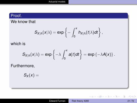
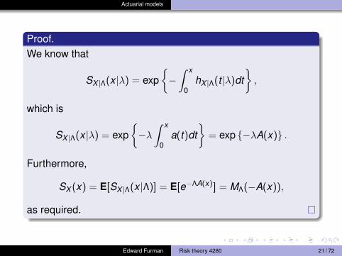
Actuarial models Proof. We know that S X |Λ (x |λ)= exp - Z x 0 h X |Λ (t |λ)dt , which is S X |Λ (x |λ)= exp -λ Z x 0 a(t )dt = exp {-λA(x )} . Furthermore, S X (x )= Edward Furman Risk theory 4280 21 / 72
-
Upload
phungkhuong -
Category
Documents
-
view
229 -
download
0
Transcript of Risk theory - Actuarial modelsefurman/risktheory2009/lecture2_1b.pdf · Actuarial models...
Actuarial models
Proof.We know that
SX |Λ(x |λ) = exp{−∫ x
0hX |Λ(t |λ)dt
},
which is
SX |Λ(x |λ) = exp{−λ∫ x
0a(t)dt
}= exp {−λA(x)} .
Furthermore,
SX (x) =
E[SX |Λ(x |Λ)] = E[e−ΛA(x)] = MΛ(−A(x)),
as required.
Edward Furman Risk theory 4280 21 / 72
Actuarial models
Proof.We know that
SX |Λ(x |λ) = exp{−∫ x
0hX |Λ(t |λ)dt
},
which is
SX |Λ(x |λ) = exp{−λ∫ x
0a(t)dt
}= exp {−λA(x)} .
Furthermore,
SX (x) = E[SX |Λ(x |Λ)] = E[e−ΛA(x)] = MΛ(−A(x)),
as required.
Edward Furman Risk theory 4280 21 / 72
Actuarial models
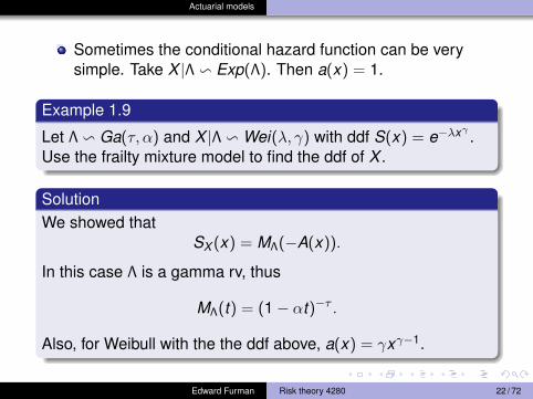
Sometimes the conditional hazard function can be verysimple.
Take X |Λ v Exp(Λ). Then a(x) = 1.
Example 1.9
Let Λ v Ga(τ, α) and X |Λ v Wei(λ, γ) with ddf S(x) = e−λxγ.
Use the frailty mixture model to find the ddf of X .
SolutionWe showed that
SX (x) = MΛ(−A(x)).
In this case Λ is a gamma rv, thus
MΛ(t) = (1− αt)−τ .
Also, for Weibull with the the ddf above, a(x) = γxγ−1.
Edward Furman Risk theory 4280 22 / 72
Actuarial models
Sometimes the conditional hazard function can be verysimple. Take X |Λ v Exp(Λ). Then a(x) = 1.
Example 1.9
Let Λ v Ga(τ, α) and X |Λ v Wei(λ, γ) with ddf S(x) = e−λxγ.
Use the frailty mixture model to find the ddf of X .
SolutionWe showed that
SX (x) = MΛ(−A(x)).
In this case Λ is a gamma rv, thus
MΛ(t) = (1− αt)−τ .
Also, for Weibull with the the ddf above, a(x) = γxγ−1.
Edward Furman Risk theory 4280 22 / 72
Actuarial models
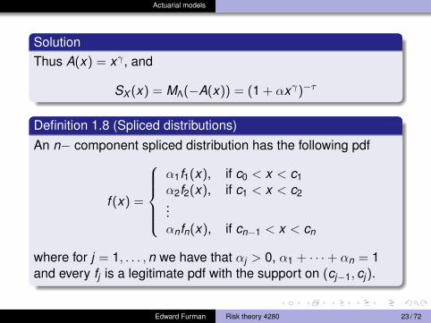
SolutionThus A(x) = xγ , and
SX (x) = MΛ(−A(x)) = (1 + αxγ)−τ
Definition 1.8 (Spliced distributions)An n− component spliced distribution has the following pdf
f (x) =
α1f1(x), if c0 < x < c1α2f2(x), if c1 < x < c2...αnfn(x), if cn−1 < x < cn
where for j = 1, . . . ,n we have that αj > 0, α1 + · · ·+ αn = 1and every fj is a legitimate pdf with the support on (cj−1, cj).
Edward Furman Risk theory 4280 23 / 72
Actuarial models
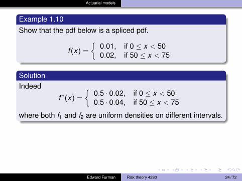
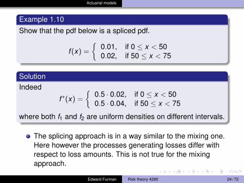
Example 1.10Show that the pdf below is a spliced pdf.
f (x) =
{0.01, if 0 ≤ x < 500.02, if 50 ≤ x < 75
SolutionIndeed
f ∗(x) =
{0.5 · 0.02, if 0 ≤ x < 500.5 · 0.04, if 50 ≤ x < 75
where both f1 and f2 are uniform densities on different intervals.
The splicing approach is in a way similar to the mixing one.Here however the processes generating losses differ withrespect to loss amounts. This is not true for the mixingapproach.
Edward Furman Risk theory 4280 24 / 72
Actuarial models
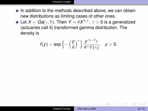
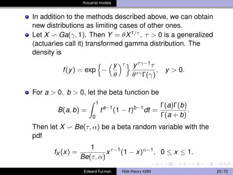
In addition to the methods described above, we can obtainnew distributions as limiting cases of other ones.
Let X v Ga(γ,1). Then Y = θX 1/τ , τ > 0 is a generalized(actuaries call it) transformed gamma distribution. Thedensity is
f (y) = exp{−(yθ
)τ} yτγ−1τ
θτγΓ(γ), y > 0.
For a > 0, b > 0, let the beta function be
B(a,b) =
∫ 1
0ta−1(1− t)b−1dt =
Γ(a)Γ(b)
Γ(a + b).
Then let X v Be(τ, α) be a beta random variable with thepdf
fX (x) =1
Be(τ, α)xτ−1(1− x)α−1, 0 ≤ x ≤ 1.
Edward Furman Risk theory 4280 25 / 72
Actuarial models
In addition to the methods described above, we can obtainnew distributions as limiting cases of other ones.Let X v Ga(γ,1). Then Y = θX 1/τ , τ > 0 is a generalized(actuaries call it) transformed gamma distribution. Thedensity is
f (y) = exp{−(yθ
)τ} yτγ−1τ
θτγΓ(γ), y > 0.
For a > 0, b > 0, let the beta function be
B(a,b) =
∫ 1
0ta−1(1− t)b−1dt =
Γ(a)Γ(b)
Γ(a + b).
Then let X v Be(τ, α) be a beta random variable with thepdf
fX (x) =1
Be(τ, α)xτ−1(1− x)α−1, 0 ≤ x ≤ 1.
Edward Furman Risk theory 4280 25 / 72
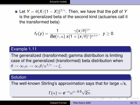
Actuarial models
Let Y = θ(X/(1− X ))1/γ . Then, we have that the pdf of Yis the generalized beta of the second kind (actuaries call itthe transformed beta)
fY (y) =1
Be(τ, α)
γ(x/θ)γτ
x(1 + (x/θ)γ)α+τ, y ≥ 0.
Example 1.11The generalized (transformed) gamma distribution is limitingcase of the generalized (transformed) beta distribution whenθ →∞,α→∞,θ/α1/γ → ξ.
SolutionThe well-known Stirling’s approximation says that for large α’s,
Γ(α) = e−ααα−0.5√
2π.
Edward Furman Risk theory 4280 26 / 72
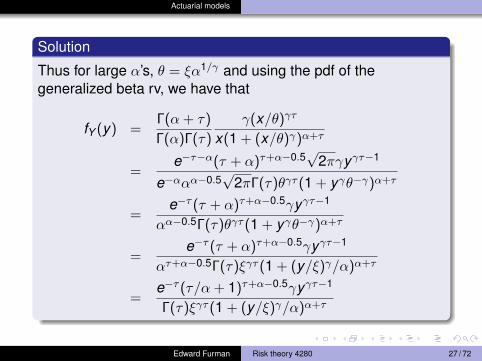
Actuarial models
Solution
Thus for large α’s, θ = ξα1/γ and using the pdf of thegeneralized beta rv, we have that
fY (y) =Γ(α + τ)
Γ(α)Γ(τ)
γ(x/θ)γτ
x(1 + (x/θ)γ)α+τ
=e−τ−α(τ + α)τ+α−0.5
√2πγyγτ−1
e−ααα−0.5√
2πΓ(τ)θγτ (1 + yγθ−γ)α+τ
=e−τ (τ + α)τ+α−0.5γyγτ−1
αα−0.5Γ(τ)θγτ (1 + yγθ−γ)α+τ
=e−τ (τ + α)τ+α−0.5γyγτ−1
ατ+α−0.5Γ(τ)ξγτ (1 + (y/ξ)γ/α)α+τ
=e−τ (τ/α + 1)τ+α−0.5γyγτ−1
Γ(τ)ξγτ (1 + (y/ξ)γ/α)α+τ
Edward Furman Risk theory 4280 27 / 72
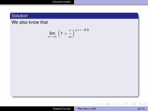
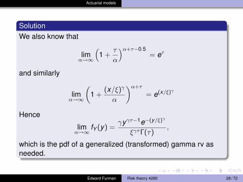
Actuarial models
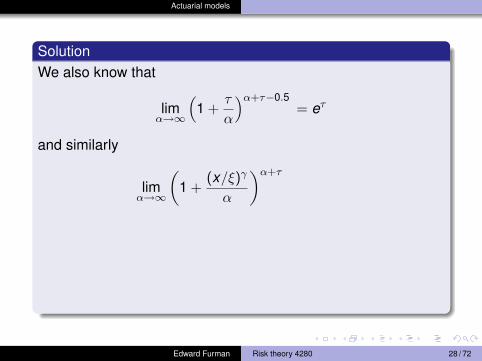
SolutionWe also know that
limα→∞
(1 +
τ
α
)α+τ−0.5
= eτ
and similarly
limα→∞
(1 +
(x/ξ)γ
α
)α+τ
= e(x/ξ)γ
Hence
limα→∞
fY (y) =γyγτ−1e−(y/ξ)γ
ξγτΓ(τ),
which is the pdf of a generalized (transformed) gamma rv asneeded.
Edward Furman Risk theory 4280 28 / 72
Actuarial models
SolutionWe also know that
limα→∞
(1 +
τ
α
)α+τ−0.5= eτ
and similarly
limα→∞
(1 +
(x/ξ)γ
α
)α+τ
= e(x/ξ)γ
Hence
limα→∞
fY (y) =γyγτ−1e−(y/ξ)γ
ξγτΓ(τ),
which is the pdf of a generalized (transformed) gamma rv asneeded.
Edward Furman Risk theory 4280 28 / 72
Actuarial models
SolutionWe also know that
limα→∞
(1 +
τ
α
)α+τ−0.5= eτ
and similarly
limα→∞
(1 +
(x/ξ)γ
α
)α+τ
= e(x/ξ)γ
Hence
limα→∞
fY (y) =γyγτ−1e−(y/ξ)γ
ξγτΓ(τ),
which is the pdf of a generalized (transformed) gamma rv asneeded.
Edward Furman Risk theory 4280 28 / 72
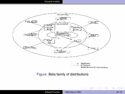
Actuarial models
Figure: Beta family of distributions
Edward Furman Risk theory 4280 29 / 72
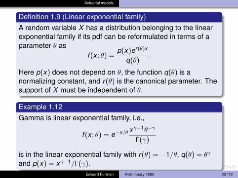
Actuarial models
Definition 1.9 (Linear exponential family)A random variable X has a distribution belonging to the linearexponential family if its pdf can be reformulated in terms of aparameter θ as
f (x ; θ) =p(x)er(θ)x
q(θ).
Here p(x) does not depend on θ, the function q(θ) is anormalizing constant, and r(θ) is the canonical parameter. Thesupport of X must be independent of θ.
Example 1.12Gamma is linear exponential family, i.e.,
f (x ; θ) = e−x/θ xγ−1θ−γ
Γ(γ)
is in the linear exponential family with r(θ) = −1/θ, q(θ) = θγ
and p(x) = xγ−1/Γ(γ).Edward Furman Risk theory 4280 30 / 72
Actuarial models
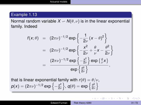
Example 1.13
Normal random variable X v N(θ, ν) is in the linear exponentialfamily. Indeed
f (x ; θ) = (2πν)−1/2 exp{− 1
2ν(x − θ)2
}= (2πν)−1/2 exp
{−x2
2ν+θ
νx − θ2
2ν
}
=(2πν)−1/2 exp
{− x2
2ν
}exp
{θν x}
exp{θ2
2ν
} ,
that is linear exponential family with r(θ) = θ/ν,p(x) = (2πν)−1/2 exp
{− x2
2ν
}, q(θ) = exp
{θ2
2ν
}
Edward Furman Risk theory 4280 31 / 72
Actuarial models
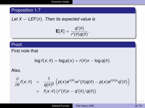
Proposition 1.7
Let X v LEF (θ). Then its expected value is
E[X ] =q′(θ)
r ′(θ)q(θ).
Proof.First note that
log f (x ; θ) = log p(x) + r(θ)x − log q(θ).
Also,
∂
∂θf (x ; θ) =
1q(θ)2
(p(x)er(θ)xr ′(θ)q(θ)− p(x)er(θ)xq′(θ)
)= f (x ; θ)
(r ′(θ)x − q′(θ)/q(θ)
)We will now differentiate the above with respect to x . ThenEdward Furman Risk theory 4280 32 / 72
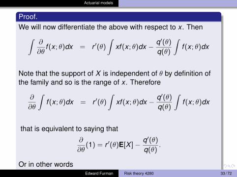
Actuarial models
Proof.We will now differentiate the above with respect to x . Then∫
∂
∂θf (x ; θ)dx = r ′(θ)
∫xf (x ; θ)dx − q′(θ)
q(θ)
∫f (x ; θ)dx
Note that the support of X is independent of θ by definition ofthe family and so is the range of x . Therefore
∂
∂θ
∫f (x ; θ)dx = r ′(θ)
∫xf (x ; θ)dx − q′(θ)
q(θ)
∫f (x ; θ)dx
that is equivalent to saying that
∂
∂θ(1) = r ′(θ)E[X ]− q′(θ)
q(θ).
Or in other wordsEdward Furman Risk theory 4280 33 / 72
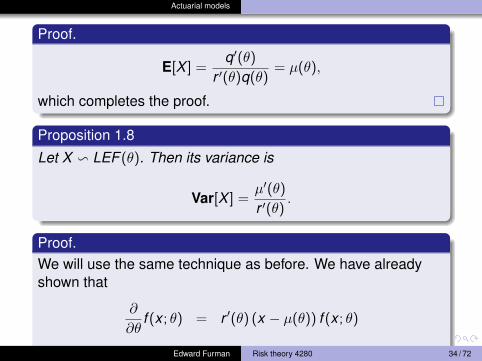
Actuarial models
Proof.
E[X ] =q′(θ)
r ′(θ)q(θ)= µ(θ),
which completes the proof.
Proposition 1.8
Let X v LEF (θ). Then its variance is
Var[X ] =µ′(θ)
r ′(θ).
Proof.We will use the same technique as before. We have alreadyshown that
∂
∂θf (x ; θ) = r ′(θ) (x − µ(θ)) f (x ; θ)
Edward Furman Risk theory 4280 34 / 72
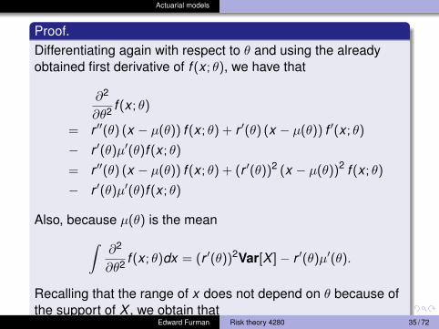
Actuarial models
Proof.Differentiating again with respect to θ and using the alreadyobtained first derivative of f (x ; θ), we have that
∂2
∂θ2 f (x ; θ)
= r ′′(θ) (x − µ(θ)) f (x ; θ) + r ′(θ) (x − µ(θ)) f ′(x ; θ)
− r ′(θ)µ′(θ)f (x ; θ)
= r ′′(θ) (x − µ(θ)) f (x ; θ) + (r ′(θ))2 (x − µ(θ))2 f (x ; θ)
− r ′(θ)µ′(θ)f (x ; θ)
Also, because µ(θ) is the mean∫∂2
∂θ2 f (x ; θ)dx = (r ′(θ))2Var[X ]− r ′(θ)µ′(θ).
Recalling that the range of x does not depend on θ because ofthe support of X , we obtain that
Edward Furman Risk theory 4280 35 / 72
Actuarial models
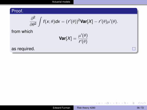
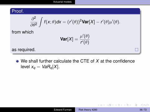
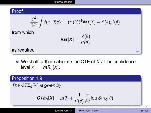
Proof.
∂2
∂θ2
∫f (x ; θ)dx = (r ′(θ))2Var[X ]− r ′(θ)µ′(θ).
from which
Var[X ] =µ′(θ)
r ′(θ)
as required.
We shall further calculate the CTE of X at the confidencelevel xq = VaRq[X ].
Proposition 1.9
The CTEq[X ] is given by
CTEq[X ] = µ(θ) +1
r ′(θ)
∂
∂θlog S(xq; θ).
Edward Furman Risk theory 4280 36 / 72
Actuarial models
Proof.
∂2
∂θ2
∫f (x ; θ)dx = (r ′(θ))2Var[X ]− r ′(θ)µ′(θ).
from which
Var[X ] =µ′(θ)
r ′(θ)
as required.
We shall further calculate the CTE of X at the confidencelevel xq = VaRq[X ].
Proposition 1.9
The CTEq[X ] is given by
CTEq[X ] = µ(θ) +1
r ′(θ)
∂
∂θlog S(xq; θ).
Edward Furman Risk theory 4280 36 / 72
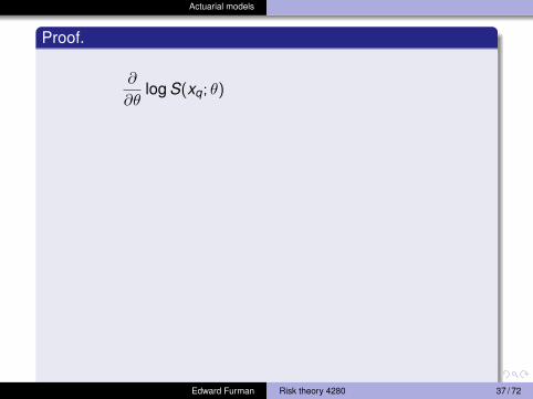
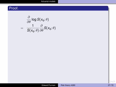
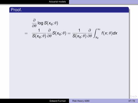
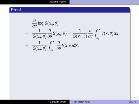
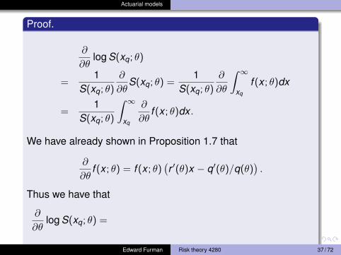
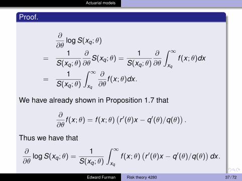
Actuarial models
Proof.
∂
∂θlog S(xq; θ)
=1
S(xq; θ)
∂
∂θS(xq; θ) =
1S(xq; θ)
∂
∂θ
∫ ∞xq
f (x ; θ)dx
=1
S(xq; θ)
∫ ∞xq
∂
∂θf (x ; θ)dx .
We have already shown in Proposition 1.7 that
∂
∂θf (x ; θ) = f (x ; θ)
(r ′(θ)x − q′(θ)/q(θ)
).
Thus we have that
∂
∂θlog S(xq; θ) =
1S(xq; θ)
∫ ∞xq
f (x ; θ)(r ′(θ)x − q′(θ)/q(θ)
)dx .
Edward Furman Risk theory 4280 37 / 72
Actuarial models
Proof.
∂
∂θlog S(xq; θ)
=1
S(xq; θ)
∂
∂θS(xq; θ)
=1
S(xq; θ)
∂
∂θ
∫ ∞xq
f (x ; θ)dx
=1
S(xq; θ)
∫ ∞xq
∂
∂θf (x ; θ)dx .
We have already shown in Proposition 1.7 that
∂
∂θf (x ; θ) = f (x ; θ)
(r ′(θ)x − q′(θ)/q(θ)
).
Thus we have that
∂
∂θlog S(xq; θ) =
1S(xq; θ)
∫ ∞xq
f (x ; θ)(r ′(θ)x − q′(θ)/q(θ)
)dx .
Edward Furman Risk theory 4280 37 / 72
Actuarial models
Proof.
∂
∂θlog S(xq; θ)
=1
S(xq; θ)
∂
∂θS(xq; θ) =
1S(xq; θ)
∂
∂θ
∫ ∞xq
f (x ; θ)dx
=1
S(xq; θ)
∫ ∞xq
∂
∂θf (x ; θ)dx .
We have already shown in Proposition 1.7 that
∂
∂θf (x ; θ) = f (x ; θ)
(r ′(θ)x − q′(θ)/q(θ)
).
Thus we have that
∂
∂θlog S(xq; θ) =
1S(xq; θ)
∫ ∞xq
f (x ; θ)(r ′(θ)x − q′(θ)/q(θ)
)dx .
Edward Furman Risk theory 4280 37 / 72
Actuarial models
Proof.
∂
∂θlog S(xq; θ)
=1
S(xq; θ)
∂
∂θS(xq; θ) =
1S(xq; θ)
∂
∂θ
∫ ∞xq
f (x ; θ)dx
=1
S(xq; θ)
∫ ∞xq
∂
∂θf (x ; θ)dx .
We have already shown in Proposition 1.7 that
∂
∂θf (x ; θ) = f (x ; θ)
(r ′(θ)x − q′(θ)/q(θ)
).
Thus we have that
∂
∂θlog S(xq; θ) =
1S(xq; θ)
∫ ∞xq
f (x ; θ)(r ′(θ)x − q′(θ)/q(θ)
)dx .
Edward Furman Risk theory 4280 37 / 72
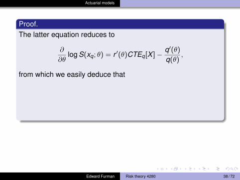
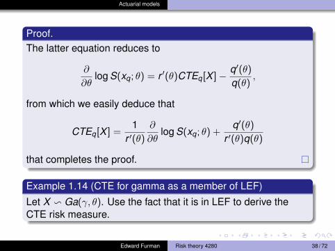
Actuarial models
Proof.The latter equation reduces to
∂
∂θlog S(xq; θ) = r ′(θ)CTEq[X ]− q′(θ)
q(θ),
from which we easily deduce that
CTEq[X ] =1
r ′(θ)
∂
∂θlog S(xq; θ) +
q′(θ)
r ′(θ)q(θ)
that completes the proof.
Example 1.14 (CTE for gamma as a member of LEF)
Let X v Ga(γ, θ). Use the fact that it is in LEF to derive theCTE risk measure.
Edward Furman Risk theory 4280 38 / 72

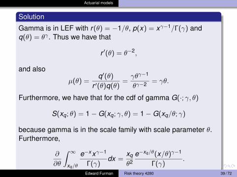
Actuarial models
Solution
Gamma is in LEF with r(θ) = −1/θ, p(x) = xγ−1/Γ(γ) andq(θ) = θγ . Thus we have that
r ′(θ) = θ−2,
and also
µ(θ) =q′(θ)
r ′(θ)q(θ)=γθγ−1
θγ−2 = γθ.
Furthermore, we have that for the cdf of gamma G(·; γ, θ)
S(xq; θ) = 1−G(xq; γ, θ) = 1−G(xq/θ; γ)
because
gamma is in the scale family with scale parameter θ.Furthermore,
∂
∂θ
∫ ∞xq/θ
e−xxγ−1
Γ(γ)dx =
xq
θ2e−xq/θ(x/θ)γ−1
Γ(γ).
Edward Furman Risk theory 4280 39 / 72
Actuarial models
Solution
Gamma is in LEF with r(θ) = −1/θ, p(x) = xγ−1/Γ(γ) andq(θ) = θγ . Thus we have that
r ′(θ) = θ−2,
and also
µ(θ) =q′(θ)
r ′(θ)q(θ)=γθγ−1
θγ−2 = γθ.
Furthermore, we have that for the cdf of gamma G(·; γ, θ)
S(xq; θ) = 1−G(xq; γ, θ) = 1−G(xq/θ; γ)
because gamma is in the scale family with scale parameter θ.Furthermore,
∂
∂θ
∫ ∞xq/θ
e−xxγ−1
Γ(γ)dx =
xq
θ2e−xq/θ(x/θ)γ−1
Γ(γ).
Edward Furman Risk theory 4280 39 / 72
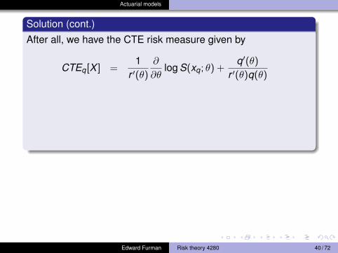
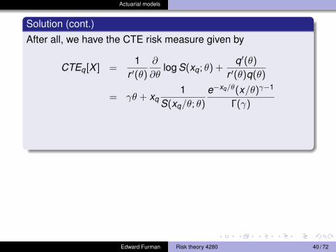
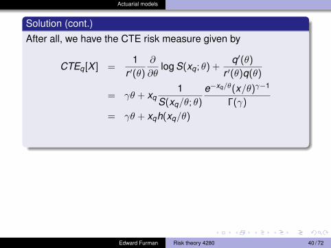
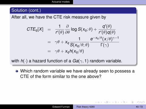
Actuarial models
Solution (cont.)After all, we have the CTE risk measure given by
CTEq[X ] =1
r ′(θ)
∂
∂θlog S(xq; θ) +
q′(θ)
r ′(θ)q(θ)
= γθ + xq1
S(xq/θ; θ)
e−xq/θ(x/θ)γ−1
Γ(γ)
= γθ + xqh(xq/θ)
with h(·) a hazard function of a Ga(γ,1) random variable.
Which random variable we have already seen to possess aCTE of the form similar to the one above?We have proved that for X v Ga(γ, θ),
CTEq[X ] = E[X ]1−G(xq; γ + 1, θ)
1−G(xq; γ, θ).
Make sure you can show the equivalence of the two.
Edward Furman Risk theory 4280 40 / 72
Actuarial models
Solution (cont.)After all, we have the CTE risk measure given by
CTEq[X ] =1
r ′(θ)
∂
∂θlog S(xq; θ) +
q′(θ)
r ′(θ)q(θ)
= γθ + xq1
S(xq/θ; θ)
e−xq/θ(x/θ)γ−1
Γ(γ)
= γθ + xqh(xq/θ)
with h(·) a hazard function of a Ga(γ,1) random variable.
Which random variable we have already seen to possess aCTE of the form similar to the one above?
We have proved that for X v Ga(γ, θ),
CTEq[X ] = E[X ]1−G(xq; γ + 1, θ)
1−G(xq; γ, θ).
Make sure you can show the equivalence of the two.
Edward Furman Risk theory 4280 40 / 72
Actuarial models
Solution (cont.)After all, we have the CTE risk measure given by
CTEq[X ] =1
r ′(θ)
∂
∂θlog S(xq; θ) +
q′(θ)
r ′(θ)q(θ)
= γθ + xq1
S(xq/θ; θ)
e−xq/θ(x/θ)γ−1
Γ(γ)
= γθ + xqh(xq/θ)
with h(·) a hazard function of a Ga(γ,1) random variable.
Which random variable we have already seen to possess aCTE of the form similar to the one above?We have proved that for X v Ga(γ, θ),
CTEq[X ] = E[X ]1−G(xq; γ + 1, θ)
1−G(xq; γ, θ).
Make sure you can show the equivalence of the two.Edward Furman Risk theory 4280 40 / 72
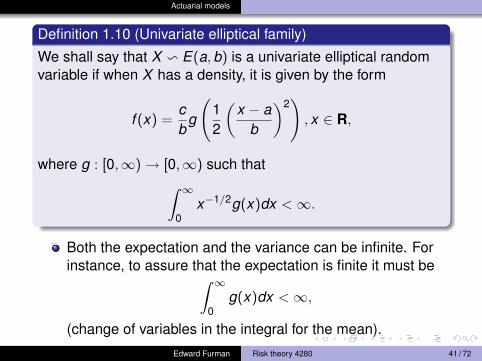
Actuarial models
Definition 1.10 (Univariate elliptical family)
We shall say that X v E(a,b) is a univariate elliptical randomvariable if when X has a density, it is given by the form
f (x) =cb
g
(12
(x − a
b
)2), x ∈ R,
where g : [0,∞)→ [0,∞) such that
∫ ∞0
x−1/2g(x)dx <∞.
Both the expectation and the variance can be infinite. Forinstance, to assure that the expectation is finite it must be∫ ∞
0g(x)dx <∞,
(change of variables in the integral for the mean).
Edward Furman Risk theory 4280 41 / 72
Actuarial models
Definition 1.10 (Univariate elliptical family)
We shall say that X v E(a,b) is a univariate elliptical randomvariable if when X has a density, it is given by the form
f (x) =cb
g
(12
(x − a
b
)2), x ∈ R,
where g : [0,∞)→ [0,∞) such that∫ ∞0
x−1/2g(x)dx <∞.
Both the expectation and the variance can be infinite. Forinstance, to assure that the expectation is finite it must be∫ ∞
0g(x)dx <∞,
(change of variables in the integral for the mean).Edward Furman Risk theory 4280 41 / 72
Actuarial models
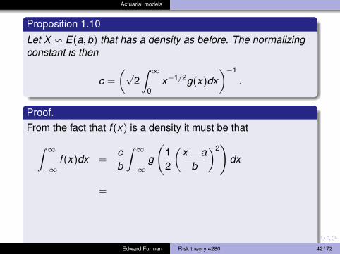
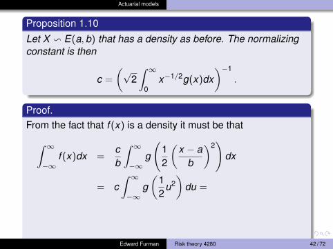
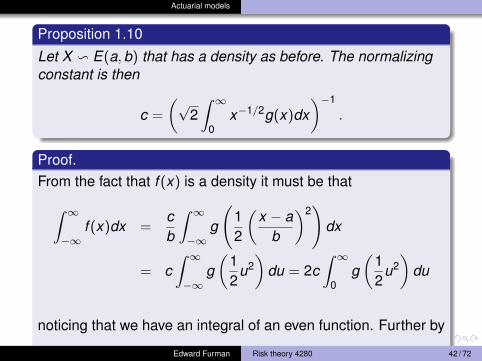
Proposition 1.10
Let X v E(a,b) that has a density as before. The normalizingconstant is then
c =
(√2∫ ∞
0x−1/2g(x)dx
)−1
.
Proof.From the fact that f (x) is a density it must be that∫ ∞
−∞f (x)dx =
cb
∫ ∞−∞
g
(12
(x − a
b
)2)
dx
= c∫ ∞−∞
g(
12
u2)
du = 2c∫ ∞
0g(
12
u2)
du
noticing that we have an integral of an even function. Further by
Edward Furman Risk theory 4280 42 / 72
Actuarial models
Proposition 1.10
Let X v E(a,b) that has a density as before. The normalizingconstant is then
c =
(√2∫ ∞
0x−1/2g(x)dx
)−1
.
Proof.From the fact that f (x) is a density it must be that∫ ∞
−∞f (x)dx =
cb
∫ ∞−∞
g
(12
(x − a
b
)2)
dx
=
c∫ ∞−∞
g(
12
u2)
du = 2c∫ ∞
0g(
12
u2)
du
noticing that we have an integral of an even function. Further by
Edward Furman Risk theory 4280 42 / 72
Actuarial models
Proposition 1.10
Let X v E(a,b) that has a density as before. The normalizingconstant is then
c =
(√2∫ ∞
0x−1/2g(x)dx
)−1
.
Proof.From the fact that f (x) is a density it must be that∫ ∞
−∞f (x)dx =
cb
∫ ∞−∞
g
(12
(x − a
b
)2)
dx
= c∫ ∞−∞
g(
12
u2)
du =
2c∫ ∞
0g(
12
u2)
du
noticing that we have an integral of an even function. Further by
Edward Furman Risk theory 4280 42 / 72
Actuarial models
Proposition 1.10
Let X v E(a,b) that has a density as before. The normalizingconstant is then
c =
(√2∫ ∞
0x−1/2g(x)dx
)−1
.
Proof.From the fact that f (x) is a density it must be that∫ ∞
−∞f (x)dx =
cb
∫ ∞−∞
g
(12
(x − a
b
)2)
dx
= c∫ ∞−∞
g(
12
u2)
du = 2c∫ ∞
0g(
12
u2)
du
noticing that we have an integral of an even function. Further by
Edward Furman Risk theory 4280 42 / 72
Actuarial models
Proof.
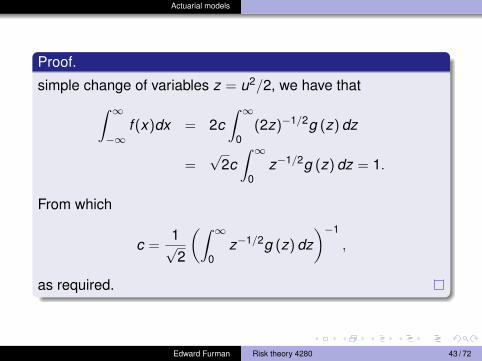
simple change of variables z = u2/2, we have that∫ ∞−∞
f (x)dx = 2c∫ ∞
0(2z)−1/2g (z) dz
=√
2c∫ ∞
0z−1/2g (z) dz = 1.
From which
c =1√2
(∫ ∞0
z−1/2g (z) dz)−1
,
as required.
Edward Furman Risk theory 4280 43 / 72
Actuarial models
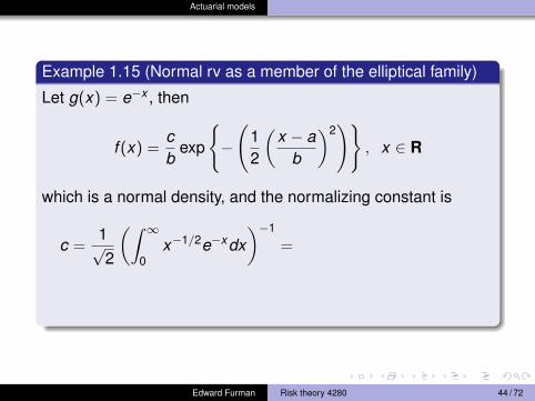
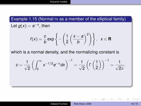
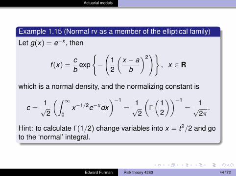
Example 1.15 (Normal rv as a member of the elliptical family)
Let g(x) = e−x , then
f (x) =cb
exp
{−
(12
(x − a
b
)2)}
, x ∈ R
which is a normal density, and the normalizing constant is
c =1√2
(∫ ∞0
x−1/2e−xdx)−1
=
1√2
(Γ
(12
))−1
=1√2π.
Hint: to calculate Γ(1/2) change variables into x = t2/2 and goto the ‘normal’ integral.
Edward Furman Risk theory 4280 44 / 72
Actuarial models
Example 1.15 (Normal rv as a member of the elliptical family)
Let g(x) = e−x , then
f (x) =cb
exp
{−
(12
(x − a
b
)2)}
, x ∈ R
which is a normal density, and the normalizing constant is
c =1√2
(∫ ∞0
x−1/2e−xdx)−1
=1√2
(Γ
(12
))−1
=1√2π.
Hint: to calculate Γ(1/2) change variables into x = t2/2 and goto the ‘normal’ integral.
Edward Furman Risk theory 4280 44 / 72
Actuarial models
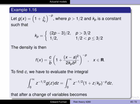
Example 1.16
Let g(x) =(
1 + xkp
)−p, where p > 1/2 and kp is a constant
such that
kp =
{(2p − 3)/2, p > 3/21/2, 1/2 < p ≤ 3/2
The density is then
f (x) =cb
(1 +
(x − a)2
2kpb2
)−p
, x ∈ R.
To find c, we have to evaluate the integral∫ ∞0
z−1/2g(z)dz =
∫ ∞0
z−1/2(1 + z/kp)−pdz,
that after a change of variables becomes
Edward Furman Risk theory 4280 45 / 72
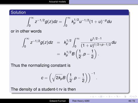
Actuarial models
Solution ∫ ∞0
z−1/2g(z)dz =
∫ ∞0
k1/2p u−1/2(1 + u)−pdu
or in other words∫ ∞0
z−1/2g(z)dz = k1/2p
∫ ∞0
u1/2−1
(1 + u)1/2+p−1/2 du
= k1/2p B
(12,p − 1
2
).
Thus the normalizing constant is
c =
(√2kpB
(12,p − 1
2
))−1
.
The density of a student-t rv is then
Edward Furman Risk theory 4280 46 / 72
Actuarial models
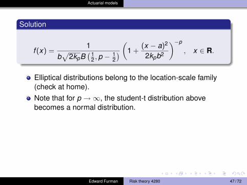
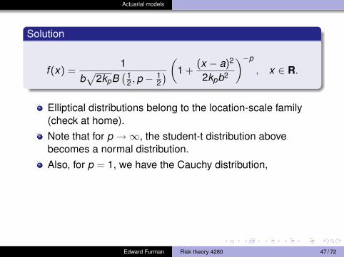
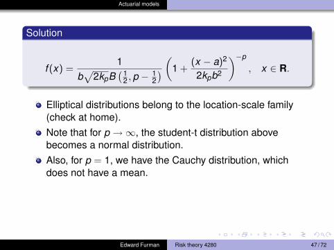
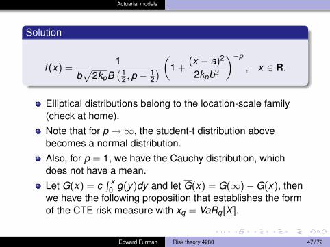
Solution
f (x) =1
b√
2kpB(1
2 ,p −12
) (1 +(x − a)2
2kpb2
)−p
, x ∈ R.
Elliptical distributions belong to the location-scale family(check at home).Note that for p →∞, the student-t distribution abovebecomes a normal distribution.
Also, for p = 1, we have the Cauchy distribution, whichdoes not have a mean.Let G(x) = c
∫ x0 g(y)dy and let G(x) = G(∞)−G(x), then
we have the following proposition that establishes the formof the CTE risk measure with xq = VaRq[X ].
Edward Furman Risk theory 4280 47 / 72
Actuarial models
Solution
f (x) =1
b√
2kpB(1
2 ,p −12
) (1 +(x − a)2
2kpb2
)−p
, x ∈ R.
Elliptical distributions belong to the location-scale family(check at home).Note that for p →∞, the student-t distribution abovebecomes a normal distribution.Also, for p = 1, we have the Cauchy distribution,
whichdoes not have a mean.Let G(x) = c
∫ x0 g(y)dy and let G(x) = G(∞)−G(x), then
we have the following proposition that establishes the formof the CTE risk measure with xq = VaRq[X ].
Edward Furman Risk theory 4280 47 / 72
Actuarial models
Solution
f (x) =1
b√
2kpB(1
2 ,p −12
) (1 +(x − a)2
2kpb2
)−p
, x ∈ R.
Elliptical distributions belong to the location-scale family(check at home).Note that for p →∞, the student-t distribution abovebecomes a normal distribution.Also, for p = 1, we have the Cauchy distribution, whichdoes not have a mean.
Let G(x) = c∫ x
0 g(y)dy and let G(x) = G(∞)−G(x), thenwe have the following proposition that establishes the formof the CTE risk measure with xq = VaRq[X ].
Edward Furman Risk theory 4280 47 / 72
Actuarial models
Solution
f (x) =1
b√
2kpB(1
2 ,p −12
) (1 +(x − a)2
2kpb2
)−p
, x ∈ R.
Elliptical distributions belong to the location-scale family(check at home).Note that for p →∞, the student-t distribution abovebecomes a normal distribution.Also, for p = 1, we have the Cauchy distribution, whichdoes not have a mean.Let G(x) = c
∫ x0 g(y)dy and let G(x) = G(∞)−G(x), then
we have the following proposition that establishes the formof the CTE risk measure with xq = VaRq[X ].
Edward Furman Risk theory 4280 47 / 72
Actuarial models
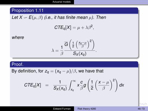
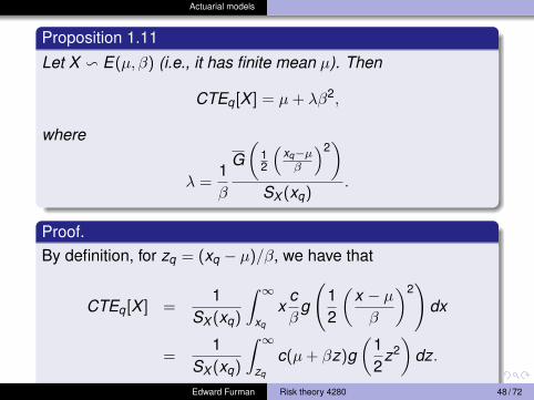
Proposition 1.11
Let X v E(µ, β) (i.e., it has finite mean µ). Then
CTEq[X ] = µ+ λβ2,
where
λ =1β
G(
12
(xq−µβ
)2)
SX (xq).
Proof.By definition, for zq = (xq − µ)/β, we have that
CTEq[X ] =1
SX (xq)
∫ ∞xq
xcβ
g
(12
(x − µβ
)2)
dx
=1
SX (xq)
∫ ∞zq
c(µ+ βz)g(
12
z2)
dz.
Edward Furman Risk theory 4280 48 / 72
Actuarial models
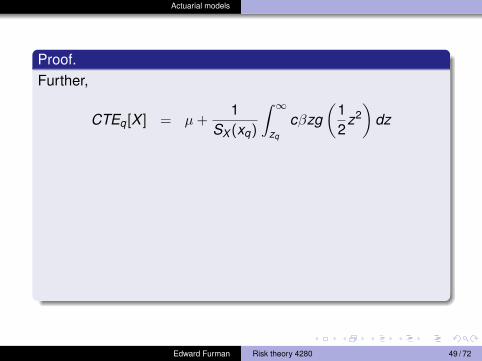
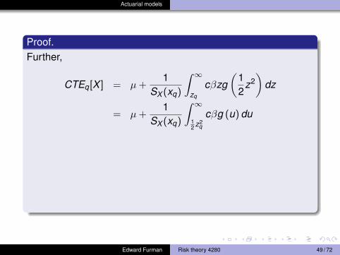
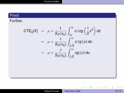
Proof.Further,
CTEq[X ] = µ+1
SX (xq)
∫ ∞zq
cβzg(
12
z2)
dz
= µ+1
SX (xq)
∫ ∞12 z2
q
cβg (u) du
= µ+β
SX (xq)
∫ ∞12 z2
q
cg (u) du
= µ+ β2 1/βSX (xq)
G(
12
z2q
),
which completes the proof.
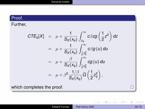
Edward Furman Risk theory 4280 49 / 72
Actuarial models
Proof.Further,
CTEq[X ] = µ+1
SX (xq)
∫ ∞zq
cβzg(
12
z2)
dz
= µ+1
SX (xq)
∫ ∞12 z2
q
cβg (u) du
= µ+β
SX (xq)
∫ ∞12 z2
q
cg (u) du
= µ+ β2 1/βSX (xq)
G(
12
z2q
),
which completes the proof.
Edward Furman Risk theory 4280 49 / 72
Actuarial models
Proof.Further,
CTEq[X ] = µ+1
SX (xq)
∫ ∞zq
cβzg(
12
z2)
dz
= µ+1
SX (xq)
∫ ∞12 z2
q
cβg (u) du
= µ+β
SX (xq)
∫ ∞12 z2
q
cg (u) du
= µ+ β2 1/βSX (xq)
G(
12
z2q
),
which completes the proof.
Edward Furman Risk theory 4280 49 / 72
Actuarial models
Proof.Further,
CTEq[X ] = µ+1
SX (xq)
∫ ∞zq
cβzg(
12
z2)
dz
= µ+1
SX (xq)
∫ ∞12 z2
q
cβg (u) du
= µ+β
SX (xq)
∫ ∞12 z2
q
cg (u) du
= µ+ β2 1/βSX (xq)
G(
12
z2q
),
which completes the proof.
Edward Furman Risk theory 4280 49 / 72
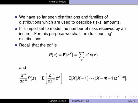
Actuarial models
We have so far seen distributions and families ofdistributions which are used to describe risks’ amounts.It is important to model the number of risks received by aninsurer. For this purpose we shall turn to ‘counting’distributions.Recall that the pgf is
P(z) = E[zX ] =∑
x
zxp(x)
and
dm
dzm P(z) = E[
dm
dzm zX]
= E[X (X−1) · · · (X−m+1)zX−m].
Edward Furman Risk theory 4280 50 / 72
Actuarial models
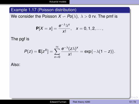
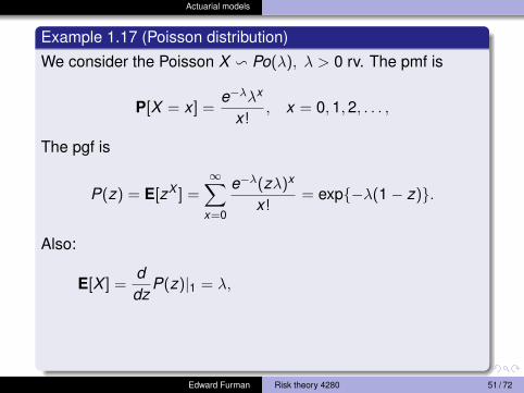
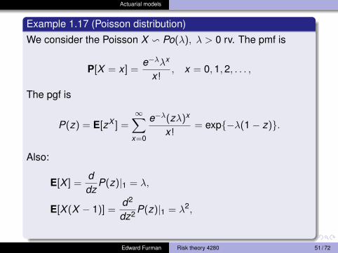
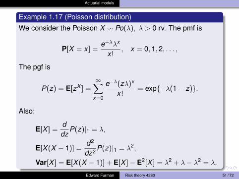
Example 1.17 (Poisson distribution)
We consider the Poisson X v Po(λ), λ > 0 rv. The pmf is
P[X = x ] =e−λλx
x!, x = 0,1,2, . . . ,
The pgf is
P(z) = E[zX ] =∞∑
x=0
e−λ(zλ)x
x!= exp{−λ(1− z)}.
Also:
E[X ] =ddz
P(z)|1 = λ,
E[X (X − 1)] =d2
dz2 P(z)|1 = λ2,
Var[X ] = E[X (X − 1)] + E[X ]− E2[X ] = λ2 + λ− λ2 = λ.
Edward Furman Risk theory 4280 51 / 72
Actuarial models
Example 1.17 (Poisson distribution)
We consider the Poisson X v Po(λ), λ > 0 rv. The pmf is
P[X = x ] =e−λλx
x!, x = 0,1,2, . . . ,
The pgf is
P(z) = E[zX ] =∞∑
x=0
e−λ(zλ)x
x!= exp{−λ(1− z)}.
Also:
E[X ] =ddz
P(z)|1 = λ,
E[X (X − 1)] =d2
dz2 P(z)|1 = λ2,
Var[X ] = E[X (X − 1)] + E[X ]− E2[X ] = λ2 + λ− λ2 = λ.
Edward Furman Risk theory 4280 51 / 72

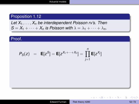
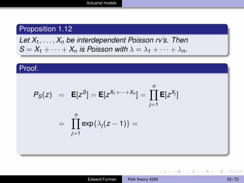
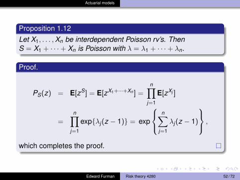
Actuarial models
Proposition 1.12Let X1, . . . ,Xn be interdependent Poisson rv’s. ThenS = X1 + · · ·+ Xn is Poisson with λ = λ1 + · · ·+ λn.
Proof.
PS(z) = E[zS] = E[zX1+···+Xn ] =
n∏j=1
E[zXj ]
=n∏
j=1
exp{λj(z − 1)} = exp
n∑
j=1
λj(z − 1)
,
which completes the proof.
Edward Furman Risk theory 4280 52 / 72
Actuarial models
Proposition 1.12Let X1, . . . ,Xn be interdependent Poisson rv’s. ThenS = X1 + · · ·+ Xn is Poisson with λ = λ1 + · · ·+ λn.
Proof.
PS(z) = E[zS] = E[zX1+···+Xn ] =n∏
j=1
E[zXj ]
=n∏
j=1
exp{λj(z − 1)} =
exp
n∑
j=1
λj(z − 1)
,
which completes the proof.
Edward Furman Risk theory 4280 52 / 72
Actuarial models
Proposition 1.12Let X1, . . . ,Xn be interdependent Poisson rv’s. ThenS = X1 + · · ·+ Xn is Poisson with λ = λ1 + · · ·+ λn.
Proof.
PS(z) = E[zS] = E[zX1+···+Xn ] =n∏
j=1
E[zXj ]
=n∏
j=1
exp{λj(z − 1)} = exp
n∑
j=1
λj(z − 1)
,
which completes the proof.
Edward Furman Risk theory 4280 52 / 72
Actuarial models
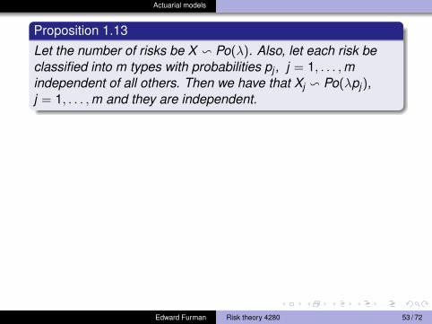
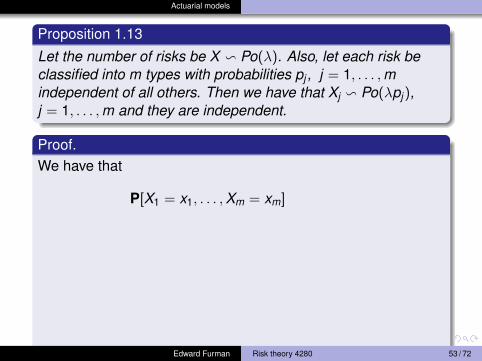
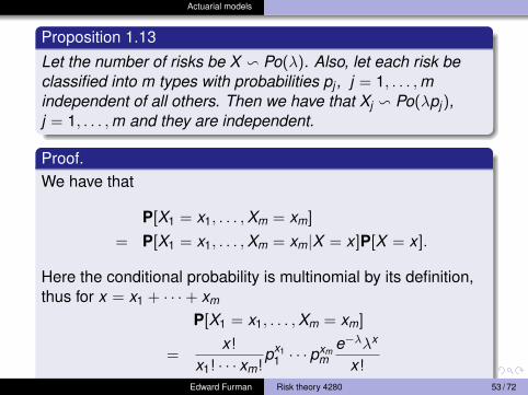
Proposition 1.13
Let the number of risks be X v Po(λ). Also, let each risk beclassified into m types with probabilities pj , j = 1, . . . ,mindependent of all others. Then we have that Xj v Po(λpj),j = 1, . . . ,m and they are independent.
Proof.We have that
P[X1 = x1, . . . ,Xm = xm]
= P[X1 = x1, . . . ,Xm = xm|X = x ]P[X = x ].
Here the conditional probability is multinomial by its definition,thus for x = x1 + · · ·+ xm
P[X1 = x1, . . . ,Xm = xm]
=x!
x1! · · · xm!px1
1 · · · pxmm
e−λλx
x!.
Edward Furman Risk theory 4280 53 / 72
Actuarial models
Proof.Hence
P[X1 = x1, . . . ,Xm = xm]
=1
x1! · · · xm!px1
1 · · · pxmm e−λλx1+···+xm
=1
x1! · · · xm!(λp1)x1 · · · (λpm)xme−
∑mj=1 λpj
=m∏
j=1
eλpj (λpj)xj
xj !.
Further, the marginal pmf is
P[Xj = xj ]
=∞∑
x=xj
P[Xj = xj ,X = x ] =∞∑
x=xj
P[Xj = xj |X = x ]P[X = x ].
Edward Furman Risk theory 4280 54 / 72