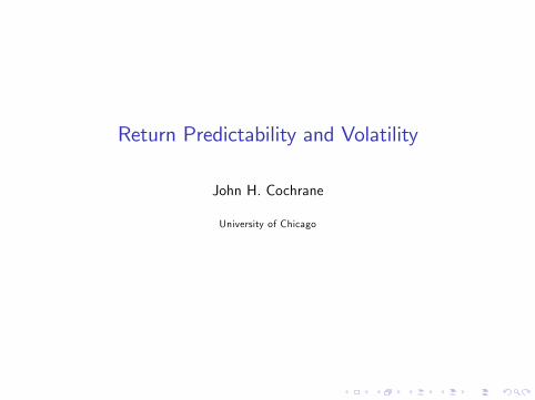
Return Predictability and Volatility

John H. Cochrane

University of Chicago

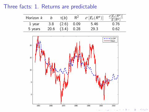
Three facts: 1. Returns are predictable

Horizon k b t(b) R2 σ [Et (Re )]σ[Et (R e )]E (R e )

1 year 3.8 (2.6) 0.09 5.46 0.765 years 20.6 (3.4) 0.28 29.3 0.62

1950 1960 1970 1980 1990 2000 2010

0

5

10

15

20

3 x D/PReturn

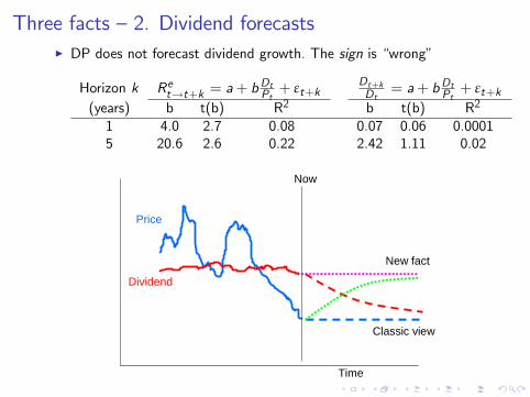
Three facts —2. Dividend forecastsI DP does not forecast dividend growth. The sign is “wrong”

Horizon k Ret→t+k = a+ bDtPt+ εt+k

Dt+kDt

= a+ bDtPt + εt+k(years) b t(b) R2 b t(b) R2

1 4.0 2.7 0.08 0.07 0.06 0.00015 20.6 2.6 0.22 2.42 1.11 0.02

Classic view

New fact

Dividend

Price

Time

Now

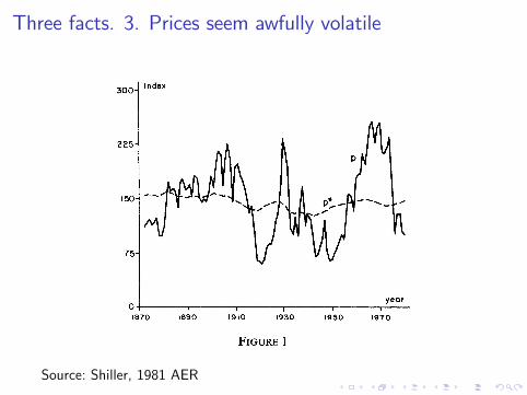
Three facts. 3. Prices seem awfully volatile

Source: Shiller, 1981 AER

Three facts - Shiller equations

P∗t =∞

∑j=1

1R jDt+j

Pt = Et (P∗t ) = Et

[∞

∑j=1

1R jDt+j

]

P∗t = Pt + εt

σ2(P∗t ) = σ2(Pt ) + σ2 (εt )

σ2(P∗t ) > σ2(Pt )

I Our task: tie all these ideas together. Along the way, develop somevery useful tools —dynamic present value identity

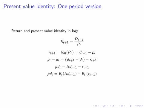
Present value identity: One period version

Return and present value identity in logs

Rt+1 =Dt+1Pt

rt+1 = log(Rt ) = dt+1 − ptpt − dt = (dt+1 − dt )− rt+1

pdt = ∆dt+1 − rt+1pdt = Et (∆dt+1)− Et (rt+1)

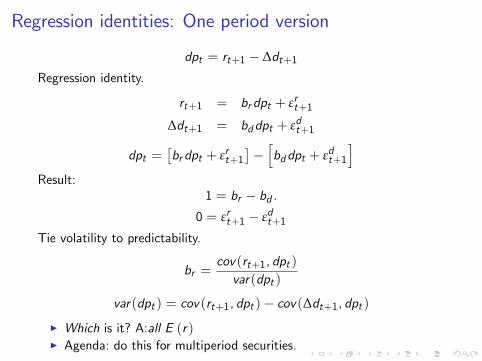
Regression identities: One period version

dpt = rt+1 − ∆dt+1Regression identity.

rt+1 = brdpt + εrt+1

∆dt+1 = bddpt + εdt+1

dpt =[brdpt + εrt+1

]−[bddpt + εdt+1

]Result:

1 = br − bd .0 = εrt+1 − εdt+1

Tie volatility to predictability.

br =cov(rt+1, dpt )var(dpt )

var(dpt ) = cov(rt+1, dpt )− cov(∆dt+1, dpt )I Which is it? A:all E (r)I Agenda: do this for multiperiod securities.

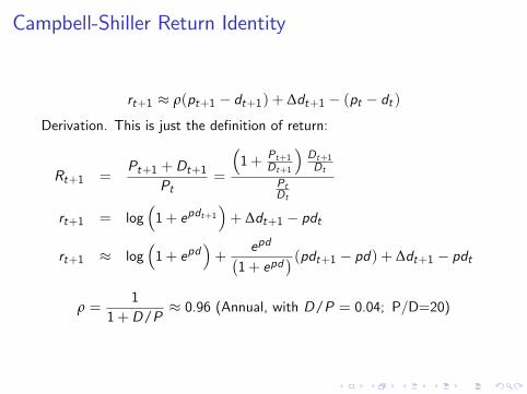
Campbell-Shiller Return Identity

rt+1 ≈ ρ(pt+1 − dt+1) + ∆dt+1 − (pt − dt )Derivation. This is just the definition of return:

Rt+1 =Pt+1 +Dt+1

Pt=

(1+ Pt+1

Dt+1

)Dt+1Dt

PtDt

rt+1 = log(1+ epdt+1

)+ ∆dt+1 − pdt

rt+1 ≈ log(1+ epd

)+

epd(1+ epd

) (pdt+1 − pd) + ∆dt+1 − pdt

ρ =1

1+D/P≈ 0.96 (Annual, with D/P = 0.04; P/D=20)

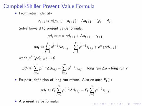
Campbell-Shiller Present Value FormulaI From return identity

rt+1 ≈ ρ(pt+1 − dt+1) + ∆dt+1 − (pt − dt )

Solve forward to present value formula.

pdt ≈ ρ× pdt+1 + ∆dt+1 − rt+1

pdt ≈k

∑j=1

ρj−1∆dt+j −k

∑j=1

ρj−1rt+j + ρk (pdt+k )

when ρk (pdt+k )→ 0

pdt ≈∞

∑j=1

ρj−1∆dt+j −∞

∑j=1

ρj−1rt+j = long run ∆d - long run r

I Ex-post; definition of long run return. Also ex ante Et (·)

pdt ≈ Et∞

∑j=1

ρj−1∆dt+j − Et∞

∑j=1

ρj−1rt+j

I A present value formula.

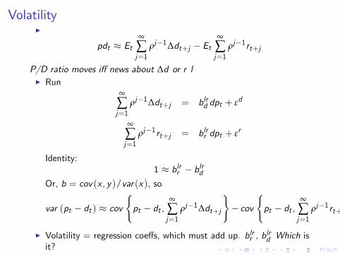
VolatilityI

pdt ≈ Et∞

∑j=1

ρj−1∆dt+j − Et∞

∑j=1

ρj−1rt+j

P/D ratio moves iff news about ∆d or r lI Run

∞

∑j=1

ρj−1∆dt+j = blrd dpt + εd

∞

∑j=1

ρj−1rt+j = blrr dpt + εr

Identity:1 ≈ blrr − blrd

Or, b = cov(x , y)/var(x), so

var (pt − dt ) ≈ cov{pt − dt ,

∞

∑j=1

ρj−1∆dt+j

}− cov

{pt − dt ,

∞

∑j=1

ρj−1rt+j

}I Volatility = regression coeffs, which must add up. blrr , b

lrd Which is

it?

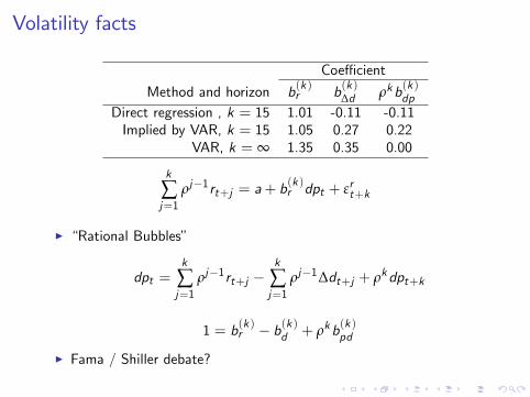
Volatility facts

Coeffi cient

Method and horizon b(k )r b(k )∆d ρkb(k )dpDirect regression , k = 15 1.01 -0.11 -0.11Implied by VAR, k = 15 1.05 0.27 0.22

VAR, k = ∞ 1.35 0.35 0.00

k

∑j=1

ρj−1rt+j = a+ b(k )r dpt + εrt+k

I “Rational Bubbles”

dpt =k

∑j=1

ρj−1rt+j −k

∑j=1

ρj−1∆dt+j + ρkdpt+k

1 = b(k )r − b(k )d + ρkb(k )pd

I Fama / Shiller debate?

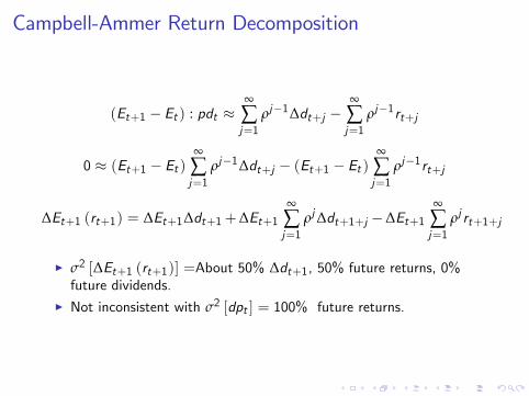
Campbell-Ammer Return Decomposition

(Et+1 − Et ) : pdt ≈∞

∑j=1

ρj−1∆dt+j −∞

∑j=1

ρj−1rt+j

0 ≈ (Et+1 − Et )∞

∑j=1

ρj−1∆dt+j − (Et+1 − Et )∞

∑j=1

ρj−1rt+j

∆Et+1 (rt+1) = ∆Et+1∆dt+1+∆Et+1∞

∑j=1

ρj∆dt+1+j −∆Et+1∞

∑j=1

ρj rt+1+j

I σ2 [∆Et+1 (rt+1)] =About 50% ∆dt+1, 50% future returns, 0%future dividends.

I Not inconsistent with σ2 [dpt ] = 100% future returns.

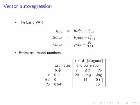
Vector autoregression

I The basic VAR

rt+1 = brdpt + εrt+1

∆dt+1 = bddpt + εdt+1

dpt+1 = φdpt + εdpt+1

I Estimates, round numbers

ε s. d. (diagonal)Estimates and correlation.b̂, φ̂ r ∆d dp

r 0.1 20 +big -big∆d 0 14 0 (!)dp 0.94 15

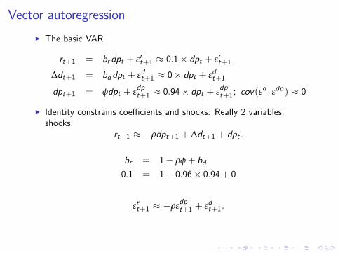
Vector autoregression

I The basic VAR

rt+1 = brdpt + εrt+1 ≈ 0.1× dpt + εrt+1

∆dt+1 = bddpt + εdt+1 ≈ 0× dpt + εdt+1

dpt+1 = φdpt + εdpt+1 ≈ 0.94× dpt + εdpt+1; cov(εd , εdp) ≈ 0

I Identity constrains coeffi cients and shocks: Really 2 variables,shocks.

rt+1 ≈ −ρdpt+1 + ∆dt+1 + dpt .

br = 1− ρφ+ bd0.1 = 1− 0.96× 0.94+ 0

εrt+1 ≈ −ρεdpt+1 + εdt+1.

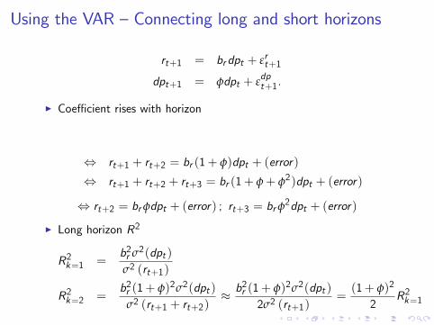
Using the VAR —Connecting long and short horizons

rt+1 = brdpt + εrt+1

dpt+1 = φdpt + εdpt+1.

I Coeffi cient rises with horizon

⇔ rt+1 + rt+2 = br (1+ φ)dpt + (error)

⇔ rt+1 + rt+2 + rt+3 = br (1+ φ+ φ2)dpt + (error)

⇔ rt+2 = brφdpt + (error) ; rt+3 = brφ2dpt + (error)

I Long horizon R2

R2k=1 =b2r σ2(dpt )σ2 (rt+1)

R2k=2 =b2r (1+ φ)2σ2(dpt )

σ2 (rt+1 + rt+2)≈ b2r (1+ φ)2σ2(dpt )

2σ2 (rt+1)=(1+ φ)2

2R2k=1

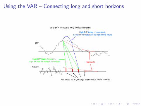
Using the VAR —Connecting long and short horizons

D/P

Return

Add these up to get large long­horizon return forecast

High D/P today forecastshigh returns for many future days

High D/P today is persistent,so return forecast will be high in the future

Forecasts

Why D/P forecasts long horizon returns

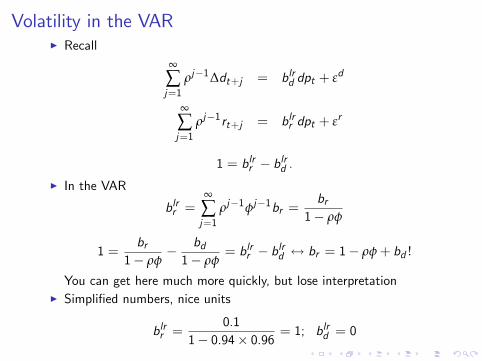
Volatility in the VARI Recall

∞

∑j=1

ρj−1∆dt+j = blrd dpt + εd

∞

∑j=1

ρj−1rt+j = blrr dpt + εr

1 = blrr − blrd .I In the VAR

blrr =∞

∑j=1

ρj−1φj−1br =br

1− ρφ

1 =br

1− ρφ− bd1− ρφ

= blrr − blrd ↔ br = 1− ρφ+ bd !

You can get here much more quickly, but lose interpretationI Simplified numbers, nice units

blrr =0.1

1− 0.94× 0.96 = 1; blrd = 0

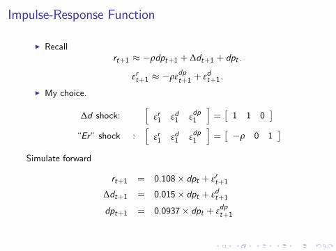
Impulse-Response Function

I Recallrt+1 ≈ −ρdpt+1 + ∆dt+1 + dpt .

εrt+1 ≈ −ρεdpt+1 + εdt+1.

I My choice.

∆d shock:[

εr1 εd1 εdp1

]=[1 1 0

]“Er”shock :

[εr1 εd1 εdp1

]=[−ρ 0 1

]Simulate forward

rt+1 = 0.108× dpt + εrt+1

∆dt+1 = 0.015× dpt + εdt+1

dpt+1 = 0.0937× dpt + εdpt+1

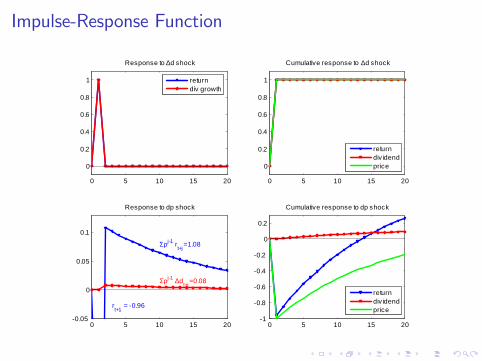
Impulse-Response Function

0 5 10 15 20

0

0.2

0.4

0.6

0.8

1

Response to ∆d shock

returndiv growth

0 5 10 15 20

0

0.2

0.4

0.6

0.8

1

Cumulative response to ∆d shock

returndiv idendprice

0 5 10 15 20­0.05

0

0.05

0.1

Response to dp shock

Σρj­1 rt+j =1.08

Σρj­1 ∆dt+j =0.08

rt+1

 = ­0.96

0 5 10 15 20­1

­0.8

­0.6

­0.4

­0.2

0

0.2

Cumulative response to dp shock

returndiv idendprice

Impulse-Response Function

1. Interpretation: how news about the future changes prices today.

1.1 εd , dividend shock with no dp change is a pure expected-cashflowshock with no change in expected returns

1.2 εdp , dp shock with no change in dividends is (almost) a purediscount-rate shock with no change in expected cashflows.

2. There is a “temporary component” to stock prices. You need tolook at both prices and dividends to see it.

Univariate vs multivariate responses

rt+1 = 0.1× rt + εt+1

0 5 10 15 200

0.2

0.4

0.6

0.8

1

Response to return shock

return

0 5 10 15 200

0.2

0.4

0.6

0.8

1

Cumulative response to return shock

return

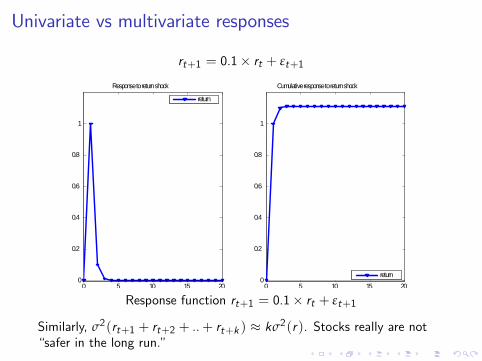
Response function rt+1 = 0.1× rt + εt+1

Similarly, σ2(rt+1 + rt+2 + ..+ rt+k ) ≈ kσ2(r). Stocks really are not“safer in the long run.”

Univariate vs multivariate responses

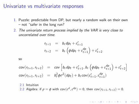
1. Puzzle: predictable from DP, but nearly a random walk on their own—not “safer in the long run?

2. The univariate return process implied by the VAR is very close touncorrelated over time.

rt+1 = brdpt + εrt+1

rt+2 = br(

φdpt + εdpt+1

)+ εrt+2

so

cov(rt+1, rt+2) = cov[brdpt + εrt+1, br

(φdpt + εdpt+1

)+ εrt+2

]cov(rt+1, rt+2) = b2r φσ2(dpt ) + br cov(εrt+1, ε

dpt+1)

2.1 Intuition2.2 Algebra: if ρ = φ with cov (εd , εdp ) = 0, then cov (rt+1, rt+2) = 0.

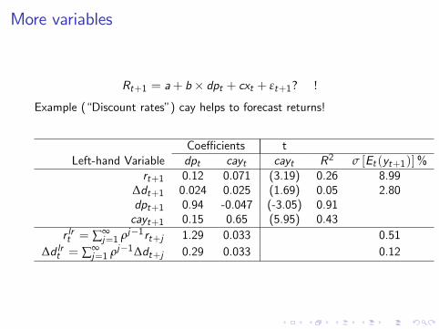
More variables

Rt+1 = a+ b× dpt + cxt + εt+1? !

Example (“Discount rates”) cay helps to forecast returns!

Coeffi cients tLeft-hand Variable dpt cayt cayt R2 σ [Et (yt+1)]%

rt+1 0.12 0.071 (3.19) 0.26 8.99∆dt+1 0.024 0.025 (1.69) 0.05 2.80dpt+1 0.94 -0.047 (-3.05) 0.91cayt+1 0.15 0.65 (5.95) 0.43

r lrt = ∑∞j=1 ρj−1rt+j 1.29 0.033 0.51

∆d lrt = ∑∞j=1 ρj−1∆dt+j 0.29 0.033 0.12

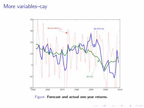
More variables—cay

1950 1960 1970 1980 1990 2000 2010­20

­10

0

10

20

30

40

dp and cay

dp only

Ac tual return rt+1

Figure: Forecast and actual one-year returns.

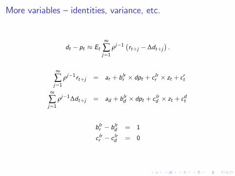
More variables — identities, variance, etc.

dt − pt ≈ Et∞

∑j=1

ρj−1(rt+j − ∆dt+j

).

∞

∑j=1

ρj−1rt+j = ar + blrr × dpt + c lrr × zt + εrt

∞

∑j=1

ρj−1∆dt+j = ad + blrd × dpt + c lrd × zt + εdt

blrr − blrd = 1

c lrr − c lrd = 0

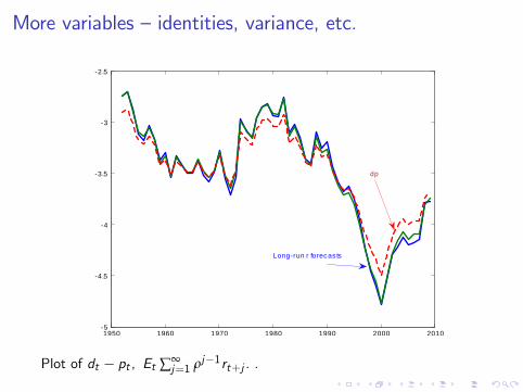
More variables — identities, variance, etc.

1950 1960 1970 1980 1990 2000 2010­5

­4.5

­4

­3.5

­3

­2.5

dp

Long­run r forecas ts

Plot of dt − pt , Et ∑∞j=1 ρj−1rt+j . .

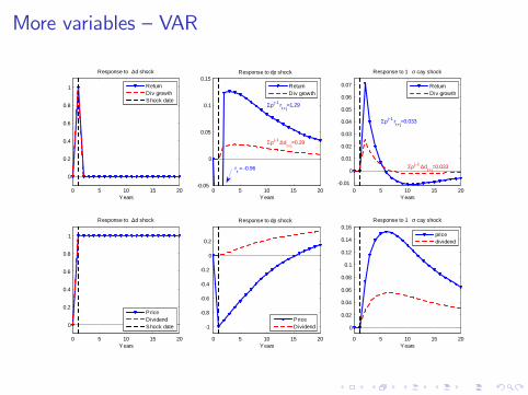
More variables —VAR

0 5 10 15 20

0

0.2

0.4

0.6

0.8

1

Years

Response to ∆d shock

ReturnDiv growthShock date

0 5 10 15 20­0.05

0

0.05

0.1

0.15

Years

Response to dp shock

Σρj ­1 rt+j

=1.29

Σρj ­1 ∆dt+j=0.29

rt = ­0.96

ReturnDiv growth

0 5 10 15 20­0.01

0

0.01

0.02

0.03

0.04

0.05

0.06

0.07

Years

Response to 1 σ cay shock

Σρj ­1 rt+j=0.033

Σρj ­1 ∆dt+j=0.033

ReturnDiv growth

0 5 10 15 20

0

0.2

0.4

0.6

0.8

1

Years

Response to ∆d shock

PriceDividendShock date

0 5 10 15 20

­1

­0.8

­0.6

­0.4

­0.2

0

0.2

Years

Response to dp shock

PriceDividend

0 5 10 15 20

0

0.02

0.04

0.06

0.08

0.1

0.12

0.14

0.16

Years

Response to 1 σ cay shock

pricedividend

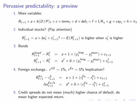
Pervasive predictability: a preview1. More variables:

Rt+1+ a+b(D/P)t + c× termt +d ×deft + f × I/Kt + g × cayt +h×πt + volatilityt +m×VIXt +n× volt ...+ εt+1

2. Individual stocks? (Pay attention)

R it+1 = a+ bxit + εit+1?↔ E (R it+1) is higher when x

it is higher

3. Bonds

Rbondt+1 − R ft = a+ 1× (y longt − y shortt ) + εt+1

R ft+1 − R ft = af + 0× (y longt − y shortt ) + εft+1

4. Foreign exchange.. rUS = 1%, rEu = 5% Implication?

REut+1 − r $t+1 = a+ 1× (rEut − r $

t ) + εt+1

∆eEu/$t+1 = ae + 0× (rEut − r $

t ) + εet+1

5. Credit spreads do not mean (much) higher chance of default, domean higher expected return.

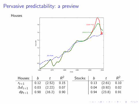
Pervasive predictability: a preview

Houses

1960 1970 1980 1990 2000 2010

6.8

7

7.2

7.4

7.6

7.8

20 x Rent

OFHE O P rice

CS W  P rice

Date

log 

scal

e

Houses: b t R2 Stocks: b t R2

rt+1 0.12 (2.52) 0.15 0.13 (2.61) 0.10∆d t+1 0.03 (2.22) 0.07 0.04 (0.92) 0.02dpt+1 0.90 (16.2) 0.90 0.94 (23.8) 0.91

Pervasive predictability/ time varying risk premiums

I Many questions!I Do the variables that forecast one thing forecast another?I What is the factor structure of expected returns across markets?I Correlation with business cycles / financial crises / economicexplanation?