Oil price shocks and stock market volatility

BANK OF GREECE

Economic Research Department – Special Studies Division

21, Ε. Venizelos Avenue

GR-102 50 Athens

Τel: +30210-320 3610

Fax: +30210-320 2432

www.bankofgreece.gr

Printed in Athens, Greece

at the Bank of Greece Printing Works.

All rights reserved. Reproduction for educational and non-commercial purposes is permitted

provided that the source is acknowledged.

ISSN 1109-6691

OIL PRICE SHOCKS AND STOCK MARKET VOLATILITY:

EVIDENCE FROM EUROPEAN DATA

Stavros Degiannakis

Bank of Greece

George Filis

Bournemouth University

Renatas Kizys

University of Portsmouth

ABSTRACT

The paper investigates the effects of oil price shocks on stock market volatility in Europe

by focusing on three measures of volatility, i.e. the conditional, the realised and the

implied volatility. The findings suggest that supply-side shocks and oil specific demand

shocks do not affect volatility, whereas, oil price changes due to aggregate demand

shocks lead to a reduction in stock market volatility. More specifically, aggregate demand

oil price shocks have significant explanatory power on both current- and forward-looking

volatilities. The results are qualitatively similar for aggregate stock market volatility and

industrial sectors’ volatilities. Finally, a robustness exercise using short- and long-run

volatility models supports the findings.

Keywords: Conditional Volatility, Realised Volatility, Implied Volatility, Oil Price

Shocks, SVAR

JEL classification: C13, C32, G10, G15, Q40

Acknowledgements: We would like to thank Heather Gibson for her constructive

suggestions which helped us to improve the clarity of the paper. The views expressed are

those of the authors and should not be interpreted as those of their respective institutions.

The authors are solely responsible for any remaining errors and deficiencies.

Correspondence:

Stavros Degiannakis

Bank of Greece

21, El. Venizelos Ave.

10250 Athens, Greece

Tel.: 0030-210-3202371

Email: [email protected]

5

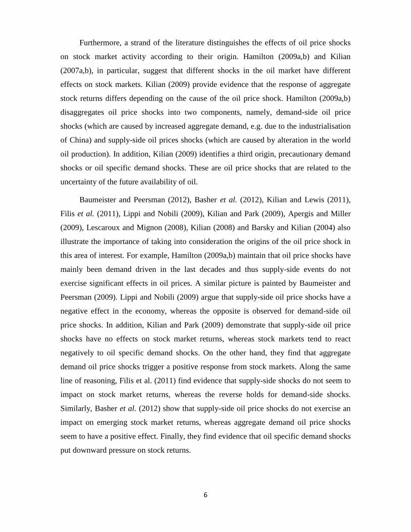
1. Introduction and brief review of the literature

There is a consensus among academics and practitioners that oil and stock

markets are often intertwined with global economic activity. Ascertaining exact nature

and sources of the linkage between oil and stock markets and global economic activity

has proved to be a promising area for researchers over the last few decades. Research

interest mainly concentrates either on the impact of oil prices on stock market

developments or the effects of oil prices on the economy. Adding to this literature, the

main objective of this paper is to conduct research into the effects of three oil price

shocks (namely, supply side shocks, aggregate demand shocks and oil specific demand

shocks) on stock market volatility, with particular reference in the European stock

market.

The seminal paper by Jones and Kaul (1996) was among the first to reveal a

negative relationship between oil prices and stock market returns. In addition, Sadorsky

(1999) concludes that oil price changes are important determinants of stock market

returns. In particular, he shows that stock markets respond negatively to a positive oil

price change. Filis (2010), Chen (2009), Miller and Ratti (2009), Park and Ratti (2008),

Driesprong et al. (2008) and Gjerde and Sættem (1999) second these findings by

Sadorsky (1999) and Jones and Kaul (1996).

The aforementioned negative relationship does not hold for stock markets operating

in oil-exporting countries. Arouri and Rault (2011) show that for the oil-exporting

countries there is a positive relationship between oil price shocks and stock market

returns. Other authors, though, do not find any relationship between oil price shocks and

stock market returns (Jammazi and Aloui, 2010; Cong et al., 2008; Haung et al., 1996).

Filis et al. (2011) provide an extensive review of the literature in the particular area.

Studies particularly focused on European stock markets reveal that positive oil

price changes tend to negatively affect stock returns; nevertheless, the exact relationship

depends on the sector. In particular, oil-related stock market sectors tend to appreciate in

the event of a positive oil price change, whereas the reverse holds for oil-intensive sectors

(see, for example, Scholtens and Yurtsever, 2012; Arouri, 2011; Arouri and Nguyen,

2010).

6

Furthermore, a strand of the literature distinguishes the effects of oil price shocks

on stock market activity according to their origin. Hamilton (2009a,b) and Kilian

(2007a,b), in particular, suggest that different shocks in the oil market have different

effects on stock markets. Kilian (2009) provide evidence that the response of aggregate

stock returns differs depending on the cause of the oil price shock. Hamilton (2009a,b)

disaggregates oil price shocks into two components, namely, demand-side oil price

shocks (which are caused by increased aggregate demand, e.g. due to the industrialisation

of China) and supply-side oil prices shocks (which are caused by alteration in the world

oil production). In addition, Kilian (2009) identifies a third origin, precautionary demand

shocks or oil specific demand shocks. These are oil price shocks that are related to the

uncertainty of the future availability of oil.

Baumeister and Peersman (2012), Basher et al. (2012), Kilian and Lewis (2011),

Filis et al. (2011), Lippi and Nobili (2009), Kilian and Park (2009), Apergis and Miller

(2009), Lescaroux and Mignon (2008), Kilian (2008) and Barsky and Kilian (2004) also

illustrate the importance of taking into consideration the origins of the oil price shock in

this area of interest. For example, Hamilton (2009a,b) maintain that oil price shocks have

mainly been demand driven in the last decades and thus supply-side events do not

exercise significant effects in oil prices. A similar picture is painted by Baumeister and

Peersman (2009). Lippi and Nobili (2009) argue that supply-side oil price shocks have a

negative effect in the economy, whereas the opposite is observed for demand-side oil

price shocks. In addition, Kilian and Park (2009) demonstrate that supply-side oil price

shocks have no effects on stock market returns, whereas stock markets tend to react

negatively to oil specific demand shocks. On the other hand, they find that aggregate

demand oil price shocks trigger a positive response from stock markets. Along the same

line of reasoning, Filis et al. (2011) find evidence that supply-side shocks do not seem to

impact on stock market returns, whereas the reverse holds for demand-side shocks.

Similarly, Basher et al. (2012) show that supply-side oil price shocks do not exercise an

impact on emerging stock market returns, whereas aggregate demand oil price shocks

seem to have a positive effect. Finally, they find evidence that oil specific demand shocks

put downward pressure on stock returns.

7

Despite the fact that evidence proposes that the origin of the oil price shock triggers

different responses from the stock markets, the majority of the literature does not

consider origin when examining its effects (see, inter alia, Arouri and Rault, 2011;

Arouri and Khuong, 2010; Bjornland, 2009; Chen, 2009; Park and Ratti, 2008).

As aforementioned, the aim of this paper is to direct the attention of the research

to the effects of the oil price shocks on stock market volatility. Studies in the early 80s

and 90s (see, for example, Pindyck, 1991 and Bernanke, 1983, among others) reveal that

increased energy prices generate uncertainty for firms, resulting in a delay in investment

decisions. Furthermore, some authors opine that oil price innovations exercise an impact

on aggregate uncertainty and they have significant negative effects on investments (see,

inter alia, Ratti et al., 2011; Rahman and Serletis, 2011; Elder and Serletis, 2010). In

addition, Bloom (2009) documents that stock market uncertainty increases after major

shocks, such as the 2001 terrorist attack in US, OPEC oil supply disruptions, etc.

Nevertheless, these studies have not considered the origins of the oil price shocks. We

argue, though, that Bloom’s choice of major shocks coincides with events that trigger

certain oil price shocks, as these have been identified by Hamilton (2009a,b) and Kilian

(2009, 2007a,b). For example, the 2001 terrorist attack in US triggered an oil specific

demand shock, whereas OPEC oil supply disruptions cause supply-side oil price shocks.

Thus, disentangling oil price shocks is of importance in understanding better stock market

uncertainty.

In addition, the literature has well established that the aforementioned firm’s

uncertainty and aggregate uncertainty can be represented by individual stock price

volatility and stock market volatility, respectively (see, for example, Baum et al., 2010

and Bloom, 2009).

Even though the characteristics of stock market volatility have been studied

extensively in the past1 , the literature remains silent on the effects of the different oil

price shocks on stock market volatility. Rather, a plethora of research output centres its

attention solely on spillover effects between the oil price volatility and stock market

1 See, among others, Xekalaki and Degiannakis (2010), Becker et al. (2007), Andersen et al. (2005),

Andersen et al. (2001) and Bollerslev et al. (1992).

8

returns and volatility or the relationship between oil price volatility and firm

investments2. This paper comes to fill this void.

More specifically, the contribution of the paper is threefold. First, it contributes to

the literature that studies the effects of three different oil price shocks – an oil supply

shock, an aggregate demand shock and an oil specific demand shock3 – on the stock

market. Unlike previous studies that examine the response of stock returns on oil price

shocks, we investigate the response of stock market volatility, as a measure of uncertainty

of stock market investments, using a Structural VAR model. Second, we provide

evidence from both aggregate stock market indices and industrial sector indices, as

according to Arouri et al. (2012, p.2) "the use of equity sector indices is, in our opinions,

advantageous because market aggregation may mask the characteristics of various

sectors". Third, in contrast to studies that mainly focus on the responses of stock market

returns in individual countries in Europe or in the US (Arouri 2011, Arouri and Nguyen

2010, and Scholtens and Yurtsever 2012 are notable exceptions), the emphasis of this

research is on the pan-European stock market.

In light of empirical evidence that underlines the relative importance of demand-

driven oil price shocks, we expect stock market volatility in Europe to be more sensitive

to an aggregate demand shock and an oil specific demand shock than to a supply-side

shock.

Three volatility measures are utilised; conditional volatility, realised volatility and

implied volatility. The use of three different volatility estimates is motivated by the fact

that part of the literature illustrates that implied volatility (a forward-looking measure) is

more informational efficient compared to other volatility estimates, which represent the

current-looking measures of volatility4. Thus, it is important to identify any differences in

their responses to oil price shocks. Koopman et al. (2005) propose that both implied

volatility and realised volatility are informationally accurate. Conversely, authors such as

Becker et al. (2007) and Corrado and Truong (2007) suggest that implied volatility

indices do not provide any incremental information compared to other volatility indices.

2 See, inter alia, Arouri et al. (2012), Henriques and Sadorsky (2011), Sadorsky (2011), Arouri et al.

(2011), Vo (2011), Malik and Ewing (2009), Chiou and Lee (2009). 3 Definitions of these shocks can be found in Kilian and Park (2009).

4 See for example Blair et al. (2001), Christensen and Prabhala (1998), Fleming (1998) and Day and Lewis

(1992).

9

Engle (2002), though, argues that there is not a simple answer as to which volatility

measure is the most accurate, as it depends upon the statistical approach adopted for the

evaluation of forecasts.

We provide evidence that supply-side shocks and oil specific demand shocks do not

affect stock market volatility, whereas, oil price changes due to aggregate demand shocks

lead to a reduction in stock market volatility. The results hold for the industrial sectors’

volatilities, as well. Prominent among our results is the finding that oil price shocks have

a qualitatively similar impact for both the current-looking volatility measures and implied

volatility, which is a forward-looking measure.

The rest of the paper is organised as follows: Section 2 presents the volatility

measures and the model used, Section 3 describes the dataset, Section 4 presents the

empirical findings of the research and Section 5 concludes the study.

2. Methodology

In the next section three measures of volatility are defined, i.e. conditional

volatility, realised volatility and implied volatility, whereas in section 2.2 the Structural

VAR model is presented.

2.1. Volatility estimates

According to the literature there are three main frameworks for measuring

volatility. The first two correspond to the current market volatility measures, whereas the

third is a forward-looking measure of volatility. In this paper we examine all three

volatility estimates.

The conditional volatility is the conditional standard deviation of the asset returns

given the most recently available information. The conditional variance process of ty

can be defined as 2

11| ttttt yVIyV , for 1tI denoting the information set

investors know when they make their investment decisions at time 1t .

The realised volatility is based on the idea of using high frequency data to

compute measures of volatility at a lower frequency, i.e. using hourly log-returns to

10

generate a measure of daily volatility. By the term monthly realized volatility we imply

the estimation of a monthly variance using daily data.

Implied volatility is the instantaneous standard deviation of the return on the

underlying asset, which would have to be input into a theoretical pricing model in order

to yield a theoretical value identical to the price of the option in the marketplace,

assuming all other inputs are known.

2.1.1. Conditional volatility

The conditional variance of the daily log-returns process, ty , is estimated with

Ding's et al. (1993) APARCH model. The APARCH model has an appealing feature that

it allows nesting tests of different types of asymmetry and functional forms (Hentschel,

1995). For instance, Laurent (2004) argues that the APARCH model nests at least seven

GARCH specifications. The asymmetric power ARCH, or APARCH model is estimated

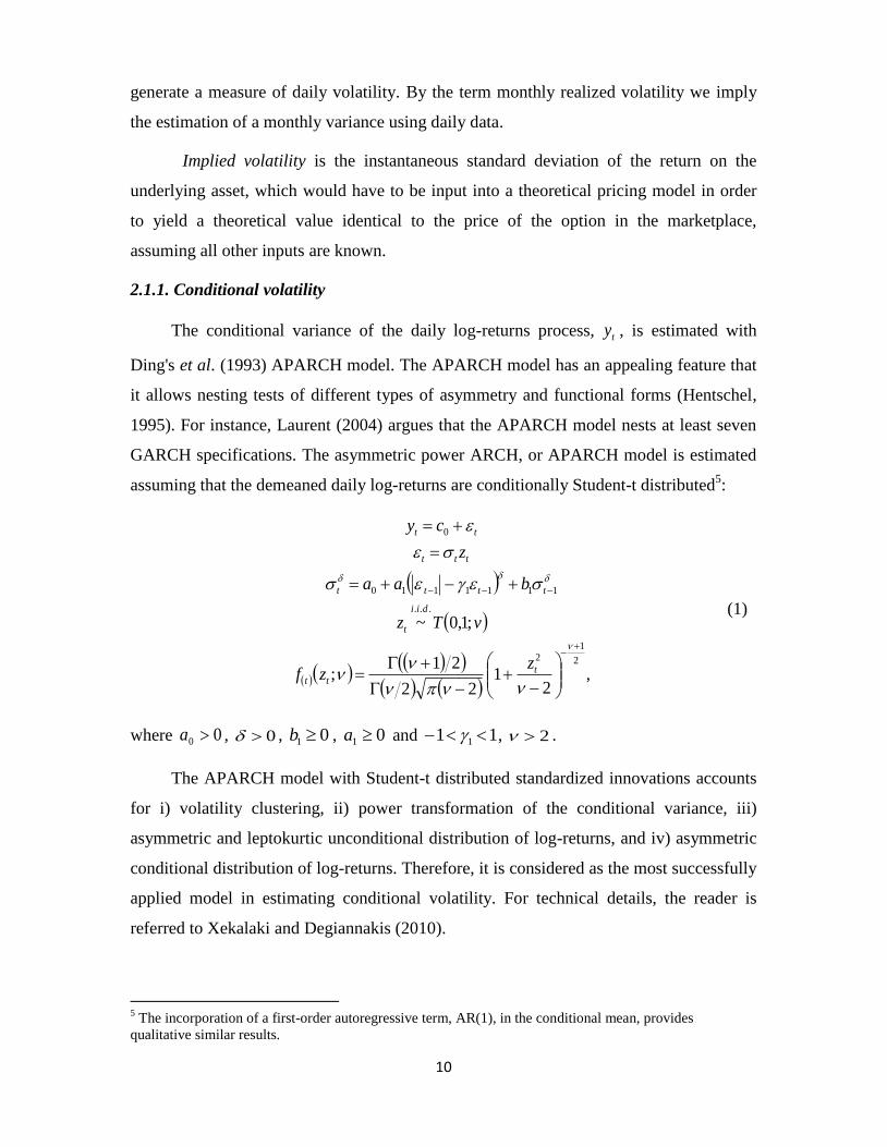
assuming that the demeaned daily log-returns are conditionally Student-t distributed5:

,

21

22

21;

;1,0~

2

12

...

1111110

0

ttt

dii

t

tttt

ttt

tt

zzf

vTz

baa

z

cy

(1)

where 00 a , 0 , 01 b , 01 a and 11 1 , 2 .

The APARCH model with Student-t distributed standardized innovations accounts

for i) volatility clustering, ii) power transformation of the conditional variance, iii)

asymmetric and leptokurtic unconditional distribution of log-returns, and iv) asymmetric

conditional distribution of log-returns. Therefore, it is considered as the most successfully

applied model in estimating conditional volatility. For technical details, the reader is

referred to Xekalaki and Degiannakis (2010).

5 The incorporation of a first-order autoregressive term, AR(1), in the conditional mean, provides

qualitative similar results.

11

The monthly conditional volatility is computed by summing the daily

conditional variances. Therefore, the annualized conditional volatility of month t , or

)(m

tCV , is computed as the square root of the sum of the conditional variances from the

16th

of the previous month up to and including the 15th

of the current month6:

1

2)( 12100j

t

m

t jCV , (2)

where 2

jt denotes the daily conditional variance for the ,...,1j trading days of month

t .

2.1.2. Realised volatility

Merton (1980) was the first to suggest the idea of using high frequency data to

compute measures of volatility at a lower frequency. The concept of the realised volatility

is based on the integrated volatility, dtt

b

a

IV

ba

22

, . The financial literature assumes

that the instantaneous logarithmic price, tplog , of a financial asset follows a diffusion

process, tdWttpd log , where t is the volatility of the instantaneous log-

returns process and tW is the standard Wiener process. The theory of quadratic

variation of semi-martingales provides a consistent estimate of the integrated volatility by

the realised variance,

1

2

, 1loglog

j

ttba jjPPRV , assuming that the time interval

ba, is partitioned in equidistant points in time; see Andersen et al. (2003) and

Barndorff-Nielsen and Shephard (2002).

For the purposes of the present study, we measure the monthly realised volatility,

partitioning the monthly time interval into daily equidistant points in time, for denoting

the number of trading days. Therefore, the annualized realised volatility of month t , or

m

tRV , is computed as the square root of the sum of the squared daily log-returns from

the 16th of the previous month up to the 15th of the current month:

6 The use of the daily observations from the 16

th of the previous month up to the 15

th of the current month is

justified by the availability of the monthly data on the 15th

of each month.

12

1

2

1loglog12100

j

tt

m

t jjPPRV . (3)

We estimate monthly volatility by summing daily volatility. However, this

measure would be biased by the number of trading days in the month. That is, volatility

in month with more trading days would be greater than volatility in any other month,

even if the volatility did not change. In order to check the robustness of the results, we

also estimate m

tRV by scaling each month’s volatility with

22 , assuming an equal

number of trading days for each month. The results remain qualitatively similar.

2.1.3. Implied volatility index - VSTOXX

Studies, see i.e. Blair et al. (2001), characterize implied volatility measures as less

informative than volatility estimated from asset returns, because they induce biases and

contain mis-specification problems. In 1993, the Chicago Board of Options Exchange

published the first implied volatility index. The computation of implied volatility indices

takes into account the latest advances in financial theory, eliminating measurement errors

that characterized the implied volatility measures.

Market participants consider the implied volatility index as an important tool for

measuring investors’ sentiment. Investors and risk managers refer to volatility indices as

fear indices or an investor fear gauge. The VSTOXX Volatility Index (which is the

volatility index for the Eurostoxx 50 Index, also named as EURO STOXX 50 Volatility

Index) measures the implied variance across all options of a given time to expiry. The

main index is designed as a rolling index at a fixed 30 days to expiry. This is achieved

using linear interpolation of the two nearest of the eight available sub-indices. The index

is calculated based on eight expiry months with a maximum time to expiry of two years.

The annualized implied volatility of month t , or m

tVSTOXX , is computed as the

average of the daily jtVSTOXX from the 16

th of the previous month up to the 15

th of the

current month:

1

21

j

t

m

t jVSTOXXVSTOXX , (4)

13

where jtVSTOXX denotes the daily implied volatility for the ,...,1j trading days of

month t . VSTOXX index is based on option prices and it is constructed by STOXX

limited7.

2.2. Structural VAR model

Using a Structural VAR framework, we examine the effects of three oil price

shocks on stock market volatility (VOL). Namely, the oil price shocks are the supply-side

shocks, the aggregate demand shocks and the oil specific demand shocks, as these are

identified from changes in world oil production (PROD), global economic activity (GEA)

and changes in oil prices (OP), respectively. VOL is the generic name of the volatility

series. For each SVAR model the volatility variable will be named after the method of

estimation (i.e. conditional, realised or implied volatility) and the name of the index

(either aggregate or industrial)8.

The structural representation of the VAR model of order p takes the following

general form:

t

p

i

itit εyAcyA

1

00 (5)

where, ty is a [4×1] vector of endogenous variables, i.e. ttttt VOLOPGEAPROD ,,,y ,

0A represents the [4x4] contemporaneous matrix, iA are [4x4] autoregressive coefficient

matrices, εt is a [4×1] vector of structural disturbances, assumed to have zero covariance

and be serially uncorrelated. The covariance matrix of the structural disturbances takes

the following form [ ]

[

]

. In order to get the reduce form

of our structural model (1) we multiply both sides with 1

0

A , such as that:

7 The interested reader can find all the necessary information about volatility index in the following link:

http://www.stoxx.com/indices/index_information.html?symbol=V2TX. 8 For example the realised volatility of the industrial sector will be named RV_INDUSTRIAL.

14

t

p

i

itit eyBay

1

0 (6)

where, 0

1

00 cAa , ii AAB

1

0

, and tt εAe1

0

, i.e. tt eAε 0 . The reduced form errors

te are linear combinations of the structural errors tε , with a covariance matrix of the form

'1

0

1

0

' DAAee ttE .

The structural disturbances can be derived by imposing suitable restrictions on 0A .

The following short-run restrictions are imposed in the model:

VOL

t

OP

t

GEA

t

PROD

t

VS

t

OSS

t

ADS

t

SS

t

e

e

e

e

aaaa

aaa

aa

a

,4

,3

,2

,1

44434241

333231

2221

11

,4

,3

,2

,1

0

00

000

where, SS=supply-side shocks, ADS=aggregate demand shock, OSS=oil specific demand

shock and VS=volatility shock.

The restrictions in the model are explained as follows. Oil production does not

respond contemporaneously to an increase/decrease in oil demand, caused by

higher/lower economic activity, due to adjustment costs in oil production. However, oil

supply disruption (a supply-side shock) can influence global economic activity, the price

of oil and stock market volatility, within the same month. Global economic activity is not

contemporaneously influenced by oil prices due to the time that is required for the world

economy to react. On the contrary, an aggregate demand shock will have an immediate

impact on oil prices and stock market volatility, considering the reaction time of the

commodities and financial markets. Turning to the oil price innovation, any increase in

the price can be driven by supply-side events, aggregate demand-side events, as well as,

oil specific demand events. Thus, oil production shocks, as well as, aggregate demand

shocks can contemporaneously trigger responses from the oil prices. In highly liquid

markets such as the European market, the stock market volatility reacts

contemporaneously to all aforementioned oil price shocks.

To proceed to the estimation of the reduced form of model (1), it is first necessary

to establish the stationarity of the variables. The ADF and PP unit root tests suggest that

15

all variables are I(0). The lag length of the VAR model was identified using the Akaike

Information Criterion (AIC). The AIC selects a VAR model with four lags9.

3. Data description

In order to estimate the volatility figures we use daily data from January 1999 to

December 2010 on aggregate European stock market indices. In particular, the stock

market index used is the Eurostoxx 50, which is Europe’s leading blue chips stock market

index and the data have been extracted from Datastream. In addition, we consider the

following industrial sectors indices, which have been constructed by Dow Jones:

Financials, Oil&Gas, Retail, Consumption Goods, Health, Industrial, Basic Materials,

Technology, Telecommunications and Utilities. The industrial sector indices data have

been extracted from Datastream. For consistency purposes we also considered the pan-

European stock market index constructed by Dow Jones. As mentioned in section 2.1,

once the daily volatility figures have been estimated, we then convert them into monthly

figures.

Furthermore, we use monthly data for the same time period for oil production, oil

prices and global economic activity. Brent crude oil is chosen, as a proxy for the world

oil price, due to the fact that this type of oil represents 60% of the world oil daily

consumption (Maghyereh, 2004). We use oil production data, as a proxy for oil supply.

Both Brent crude oil price and oil production data have been extracted from the Energy

Information Administration. Finally, we adopt Kilian’s (2009) measurement of the global

economic activity based on dry cargo freight rates10

. Prices are expressed in dollar terms

and are transformed in log-returns.

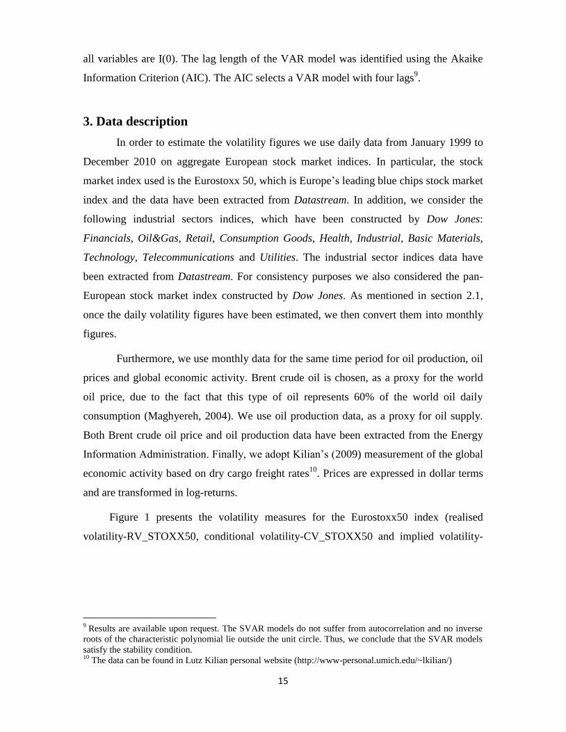
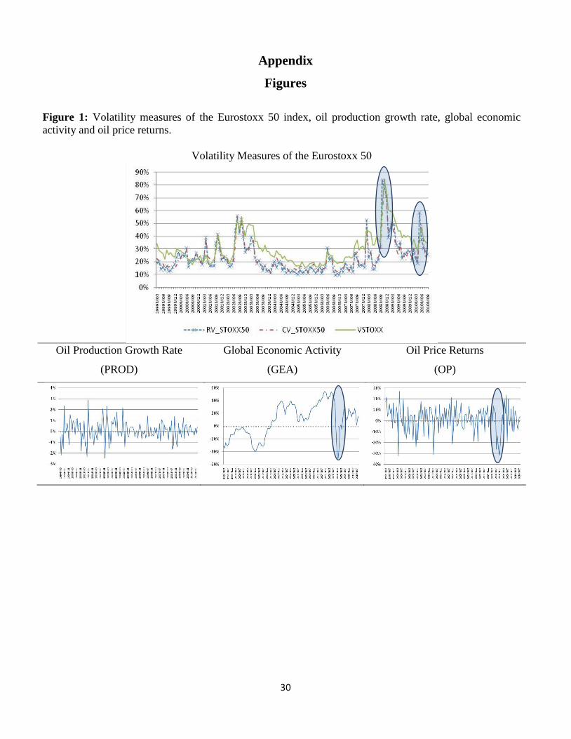
Figure 1 presents the volatility measures for the Eurostoxx50 index (realised

volatility-RV_STOXX50, conditional volatility-CV_STOXX50 and implied volatility-

9 Results are available upon request. The SVAR models do not suffer from autocorrelation and no inverse

roots of the characteristic polynomial lie outside the unit circle. Thus, we conclude that the SVAR models

satisfy the stability condition. 10

The data can be found in Lutz Kilian personal website (http://www-personal.umich.edu/~lkilian/)

16

VSTOXX), the growth rate of world oil production, global economic activity and oil

price returns11

.

[FIGURE 1 HERE]

It is immediately apparent that volatility (in all three expressions) reaches a peak

near the end of 2008 and again in May 2010. These periods coincide with the world

financial crisis and the Greek debt crisis, respectively. Similar patterns are observed in

the volatility measures of the pan-European stock market index by Dow Jones and of all

industrial sectors’ indices (not presented visually here, though). During 2008, we also

observe a trough in global economic activity and extreme negative returns for the oil

prices. This period has been also characterised by demand driven oil price shocks. These

preliminary findings may suggest that stock market volatility responds heavily to demand

driven oil price shocks. Nevertheless, the impulse responses from the SVAR model will

provide us with a clearer picture.

Furthermore, Table 1 presents some descriptive statistics for the volatility

measures of the Eurostoxx 50 index and the three oil variables. The mean values of the

realised volatility and conditional volatility are very close, whereas the VSTOXX mean

value is higher. In addition, all volatility measures exhibit significant variation over time

which is evident from the minimum, maximum and standard deviation statistics.

Naturally, the volatility measures are positively skewed and leptokurtic.

[TABLE 1 HERE]

As far as the oil variables are concerned, the global economic activity is the most

volatile, followed by oil price returns. Both variables are positively skewed, whereas oil

production growth rates are negatively skewed. The skewness measures suggest that there

are more negative oil log-returns and changes in the global economic activity, whereas

the oil production exhibits more positive returns.

11

The volatility graphs for the pan-European stock market index and the industrial sectors indices are

available upon request.

17

4. Estimation results

The purpose of the SVAR model is to examine the dynamic adjustments of each

of the variables to exogenous stochastic structural shocks (see, inter alia, Bjornland and

Leitemo, 2009; Kilian and Park, 2009). Thus, next we present the SVAR model findings

for the volatility indices of the Eurostoxx50 and the industrial sectors in terms of the

impulse response functions (IRF) and the variance decomposition12

.

Section 4.1 describes the estimation results based on current-looking measures of

stock market volatility (conditional and realised volatilities). The results for the aggregate

stock market and industrial sector indices are summarised in Sections 4.1.1 and 4.1.2,

respectively. Section 4.2 describes the estimation results based on the forward-looking

measure of stock market volatility (implied volatility).

4.1. Current-looking volatility measures

4.1.1. Aggregate European stock market indices

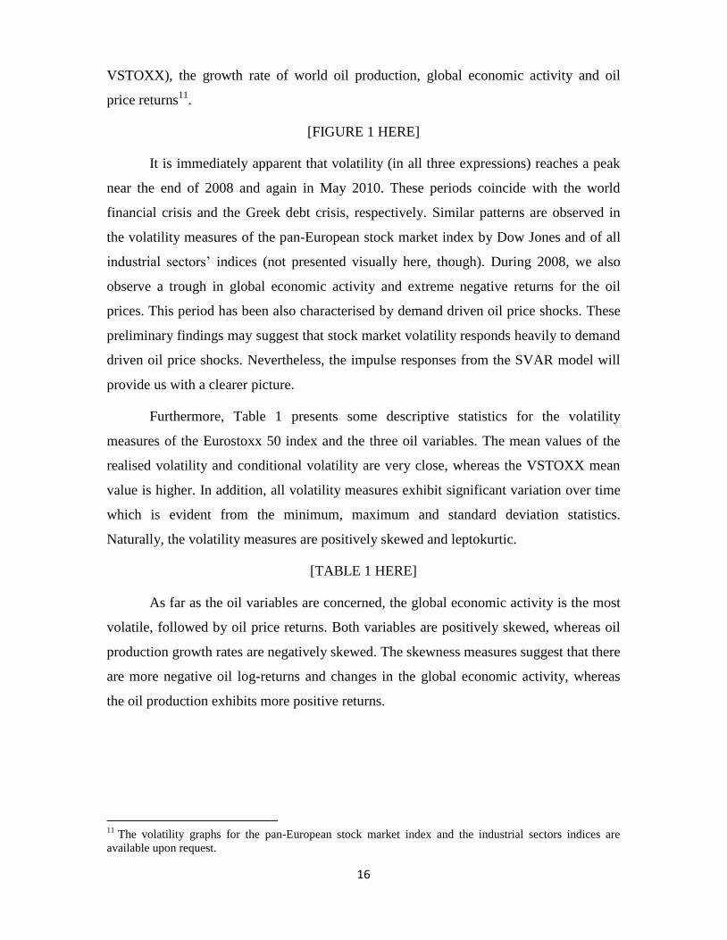
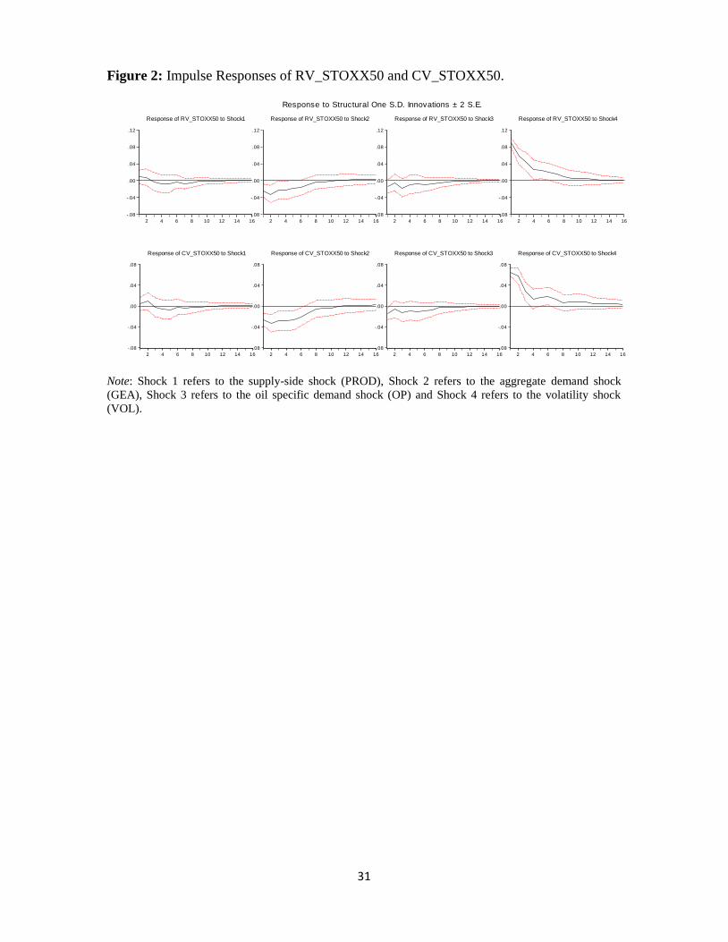
The impulse responses (Figure 2) depict that the reaction of the volatility measures

of the Eurostoxx50 index to the three oil shocks differ quite substantially.

[FIGURE 2 HERE]

Changes in world oil production do not exercise any significant impact on stock

market volatility. The argument that OPEC’s decisions on oil production levels do not

impact stock markets nowadays, finds support here. Thus, this finding does not come as a

surprise. Furthermore, the fact that stock market volatility does not react to supply-side

oil prices shocks complements the evidence provided by Basher et al. (2012), Filis et al.

(2011) and Kilian and Park (2009), who argue that changes in oil production do not affect

stock price returns. A similar observation can be made for the oil specific demand shock,

as its effect is not significant on any volatility measure. A plausible explanation of this

result lies in the nature of firms’ responses to oil price changes. We argue that firms,

nowadays, engage in effective hedging strategies which reduce the effects of adverse oil

price movements (Arouri, 2011), mainly caused by idiosyncratic oil price shocks (or oil

12

The SVAR results for the pan-European stock market index constructed by Dow Jones® are qualitatively

similar and thus they are not presented here. They are available upon request.

18

specific demand shocks). On the contrary, increases in world aggregate demand, which

implies increased economic activity, tend to reduce stock market volatility, as expected.

A positive aggregate demand shock can be regarded as good news for the stock market.

In the event of a positive aggregate demand shock, uncertainty about future cash flows

decreases, driving down stock market volatility. One can also argue positive news about

global economic activity is associated with a more stable business environment, which, in

turn, reduces uncertainty in the market. From an opposite angle, Bloom (2009) has shown

that negative news about the global economic activity, such as those during the Asian

crisis in 1997 and the credit crunch in 2008, tend to increase stock market volatility. In

general, stock markets tend to respond favourably when world economic developments

are positive. The preliminary findings had already provided an initial idea about the

inverse link between aggregate demand oil price shocks and stock market volatility.

Overall, the response is significant for about 6 months and dynamic convergence is

achieved after 12 months after the shock, for both volatility measures.

With regard to the variance decomposition (Table 2), we observe that the effects

of the supply-side and oil specific demand shocks are very small and it further suggests

that these shocks do not exercise an impact on stock market volatility. Furthermore, the

effects of the aggregate demand shocks are small in the short-run; however their

explanatory power exhibits an increasing pattern as the forecasting window increases.

This is suggestive of the fact that aggregate demand shocks have a very important role in

the European stock market volatility.

[TABLE 2 HERE]

In more detail, about 9%-18% (depending on the volatility measure) of the

variation in the volatility of the Eurostoxx50 index is associated with the oil price shocks,

during the first few months. In a period of 24 months a total of 24%-38% of the

variability of the volatility is explained by the oil price shocks. The main contributor to

this variability for both volatility measures is the aggregate demand oil price shock.

Linking these findings with the evidence on stock market returns (see, for example,

Kilian and Park, 2009; Hamilton, 2009a,b) suggests that supply-side shocks do not seem

to influence any of the stock markets characteristics (i.e. returns and volatilities), whereas

demand-side shocks – and in particular the aggregate demand oil price shocks – do.

19

Overall, the results suggest that increases in oil prices due to increased global

economic activity (aggregate demand shock) reduce stock market volatility, as global

economic activity is regarded as positive information by the stock markets.

4.1.2. European industrial sectors

Having analysed the effects of the three oil shocks on the aggregate stock market

volatility, we proceed to the analysis of these effects on the industrial sectors13

.

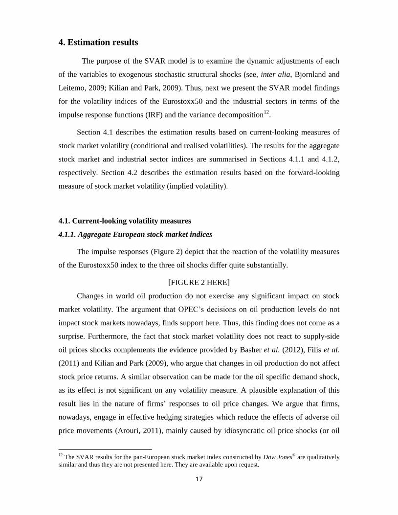
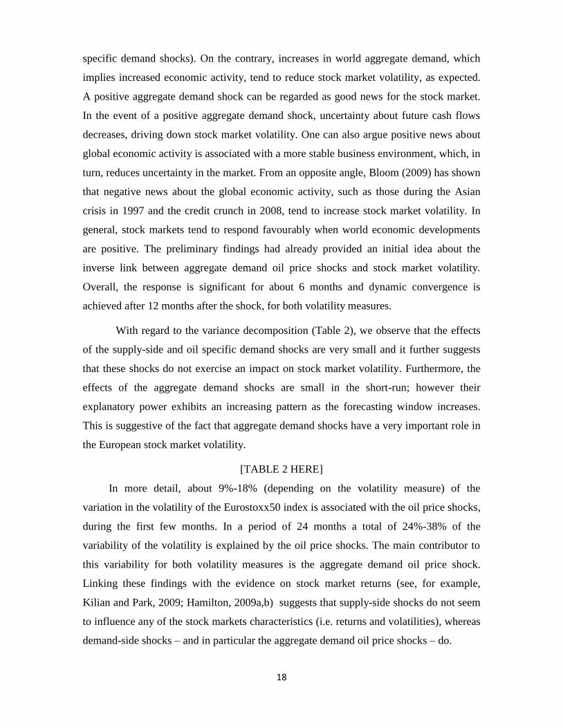
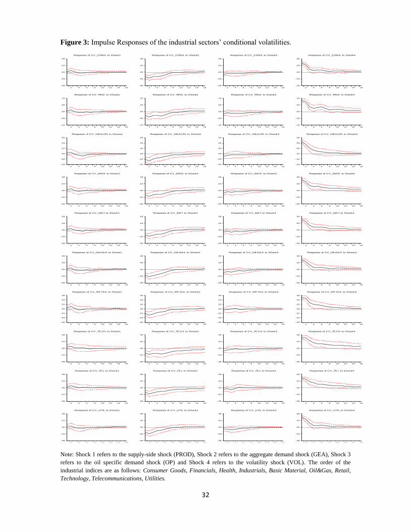
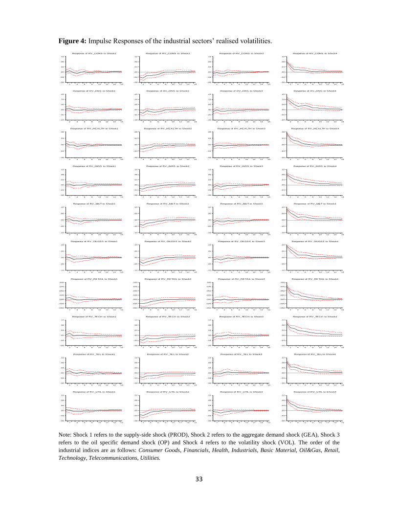
The impulse responses (Figure 3 and 4) suggest that the reaction of the volatility

measures for the industrial sectors on the three oil shocks is similar to those of the

Eurostoxx50 volatility measures. More specifically, the aggregate demand shock

exercises a significant negative effect on industrial sectors’ volatility (the same result

holds for both the realised volatility and the conditional volatility). The supply-side oil

price shocks and the oil specific demand shocks do not seem to influence any of the

sectors’ realised or conditional volatilities.

[FIGURE 3 HERE]

[FIGURE 4 HERE]

The only exemption is the Oil&Gas sector. Both the realised and conditional

volatility of the Oil&Gas sector respond negatively to the two demand-side shocks (i.e.

aggregate demand shock and oil specific demand shock). This finding is expected since

any increase in oil price is received as positive news for the companies listed in the

Oil&Gas sector. The effects remain significant for about 3-4 months and they are fully

absorbed after 8 to10 months. It could be argued that supply-side shocks should also

benefit the Oil&Gas sector; nevertheless, we cannot find such evidence in this study.

Overall, the findings suggest that disruptions or increases in world oil production

do not provide any information for the volatility of any sector, even the Oil&Gas one.

The opposite holds for the aggregate demand oil price shocks.

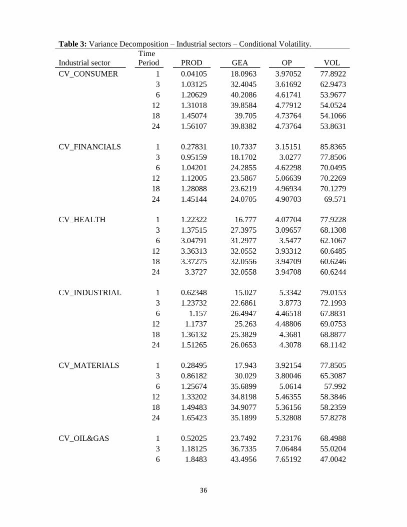
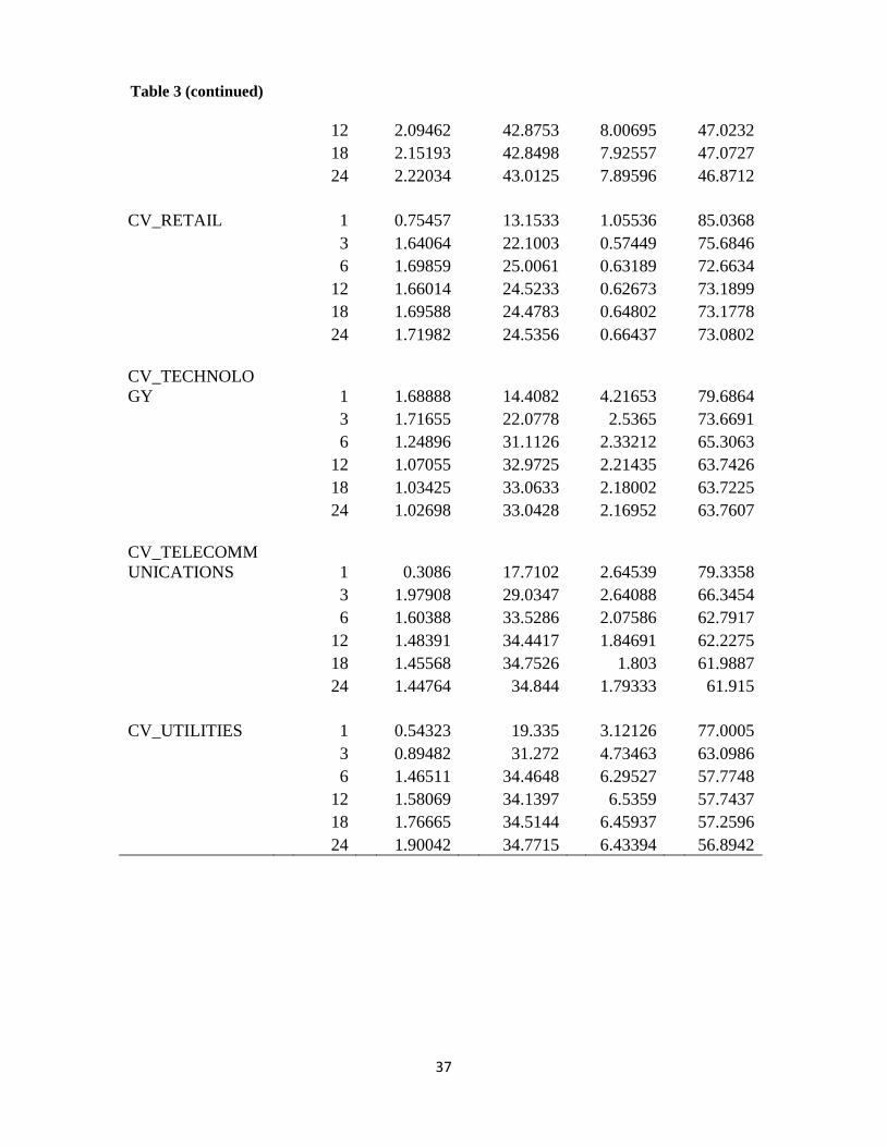
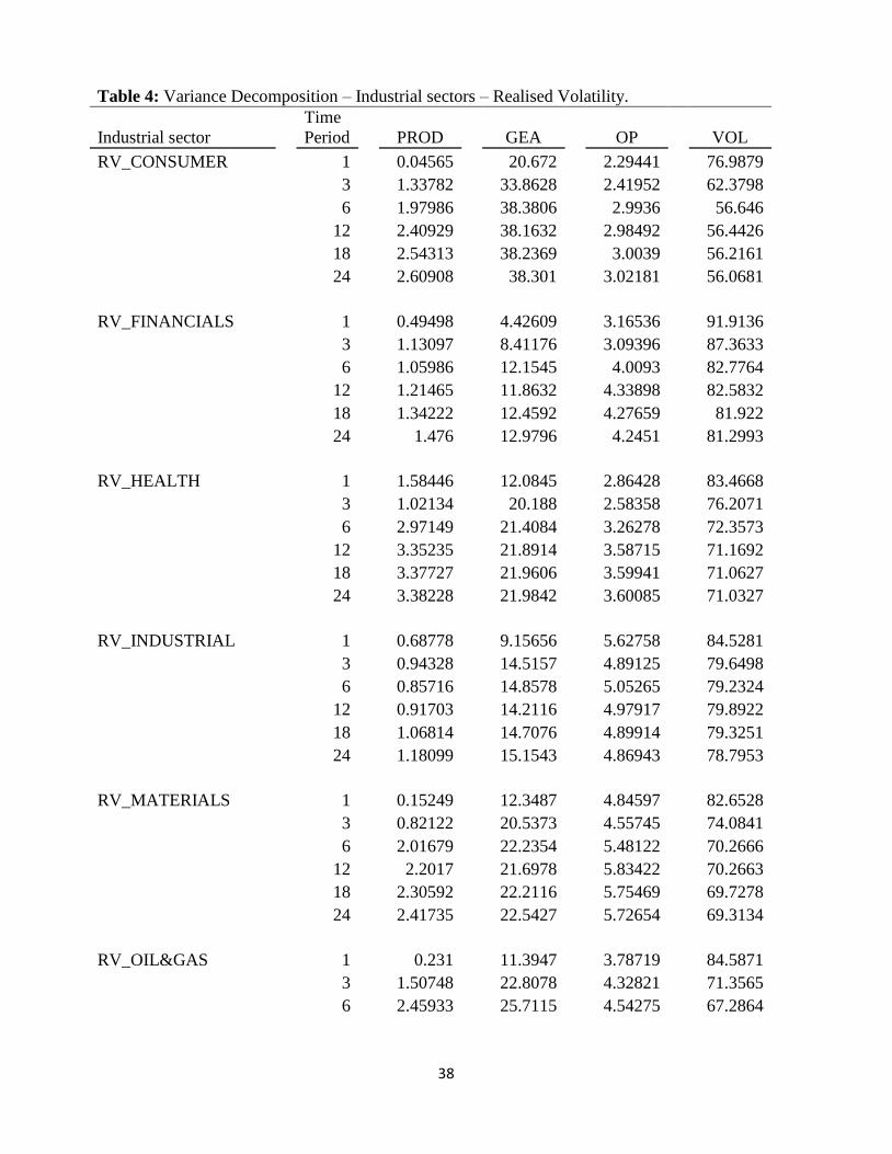
The variance decomposition analysis (Table 3 and 4) illustrates that the three oil

price shocks exercise the highest influence on the RV_OIL&GAS and CV_OIL&GAS

(about 53%), as expected, and it is followed by the RV_CONSUMPTION and

13

The descriptive statistics and figures of the industrial sectors’ volatility measures are available upon

request.

20

CV_CONSUMPTION (about 40%). The latter is expected to be influenced heavily from

the oil price shocks considering that Europe is mainly an oil importing region. Regarding

the remaining industrial indices, the three oil price shocks explain about 10%-20% of the

variability of their volatility. The lowest influenced is observed in the realised and

conditional volatility of the Financials sector (about 10%), suggesting that the Financials

sector’s volatility is mainly influenced by other variables, rather than the oil price shocks.

The main contributor of this influence, in all cases, is the aggregate demand shock, a

similar finding with the aggregate European stock market volatility.

[TABLE 3 HERE]

[TABLE 4 HERE]

4.2. Forward-looking volatility measure

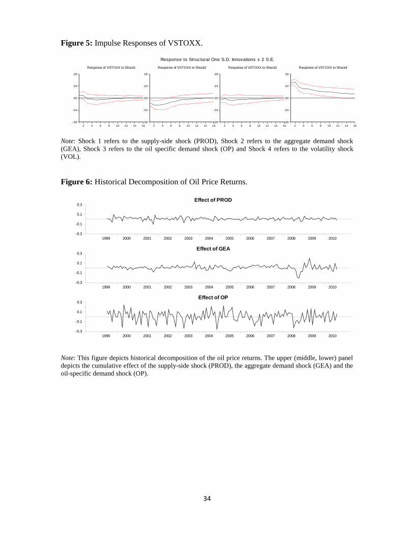
The impulse responses (Figure 5) of the Eurostoxx50 implied volatility (VSTOXX)

measure is essential the same as those produced by the conditional and realised

volatilities.

[FIGURE 5 HERE]

Again, both supply-side oil price shocks and oil specific demand shocks do not

exercise any significant impact on implied volatility, whereas positive aggregate demand

oil price shocks trigger a negative response.

In terms of the variance decomposition (Table 5), we observe that the explanatory

power of the three oil price shocks for implied volatility exhibits a peak in the medium-

term and starts to decline thereafter until it reaches a stable level after 24 months.

[TABLE 5 HERE]

More specifically, in the first month about 9% of the variation in the implied

volatility is associated with the oil price shocks, whereas in a period of 6-12 months this

figure increases to an average of 22%. The main contributor to this variability is the

aggregate demand oil price shock, as also suggested by the conditional and realised

volatilities.

Comparing the results among the three volatility measures, we observe that these

measures provide qualitatively and quantitatively similar information. Hence, the implied

volatility index (a forward-looking volatility measure) does not provide additional

21

information compared to the conditional and realised volatility measures, which estimate

the market volatility at the current time. This is a very interesting finding considering that

several aforementioned studies have concluded that implied volatility indices provide

superior information (see Xekalaki and Degiannakis, 2010; Becker et al., 2007; Andersen

et al., 2005; Andersen et al., 2001 and Bollerslev et al., 1992). Despite the fact that this

result may come as a surprise, it is not inexplicable. It is worth noting that this result does

not contradict the forward-looking feature of the implied volatility measure. The impulse

responses of the current-looking volatility measures suggest that the effects of the

aggregate demand oil price shocks do not fade immediately, but rather they require about

12 months to be fully absorbed. This means that the impact remains for the future months

and this is what it is captured by the implied volatility response to the aggregate demand

oil price shocks. The uncharacteristically prolonged response of the implied volatility is

also an artifact of its long memory, stemming from the estimate of equations 7 and 8 in

Section 5.

5. Robustness checks

In order to test for the robustness of our results a battery of alternative approaches

has been employed. More specifically, we estimate two volatility models (one with short

memory and one with long memory) and we examine whether the aggregate demand oil

price shock series has explanatory power for stock market volatility. The choice of the

aggregate demand oil price shock series is justified by the fact that it was the only oil

price shock that had a significant effect on stock market volatility, based on the impulse

response functions. Because stock market volatility is found to be invariant to the supply-

side shock and the oil specific demand shock, we deliberately discard these two shocks

from our robustness exercise.

First, we construct the aggregate demand oil price shock series (ADS). In order to

achieve that we proceed to a historical decomposition of the effects of all three oil price

shocks on the oil price returns14

.

14

See Burbidge and Harrison (1985) and Kilian and Park (2009) for a detailed description of the historical

decomposition.

22

Having decomposed the oil price returns series into the three components (i.e. the

three oil price shocks), the ADS series will represent the cumulative effect of the

aggregate demand shocks on oil price log-returns. The historical decomposition of the

oil-price returns is depicted in Figure 6. The upper, middle and lower panel depicts the

cumulative effect of the supply-side shock, the aggregate demand shock and the oil-

specific demand shock on the oil price returns, respectively.

[FIGURE 6 HERE]

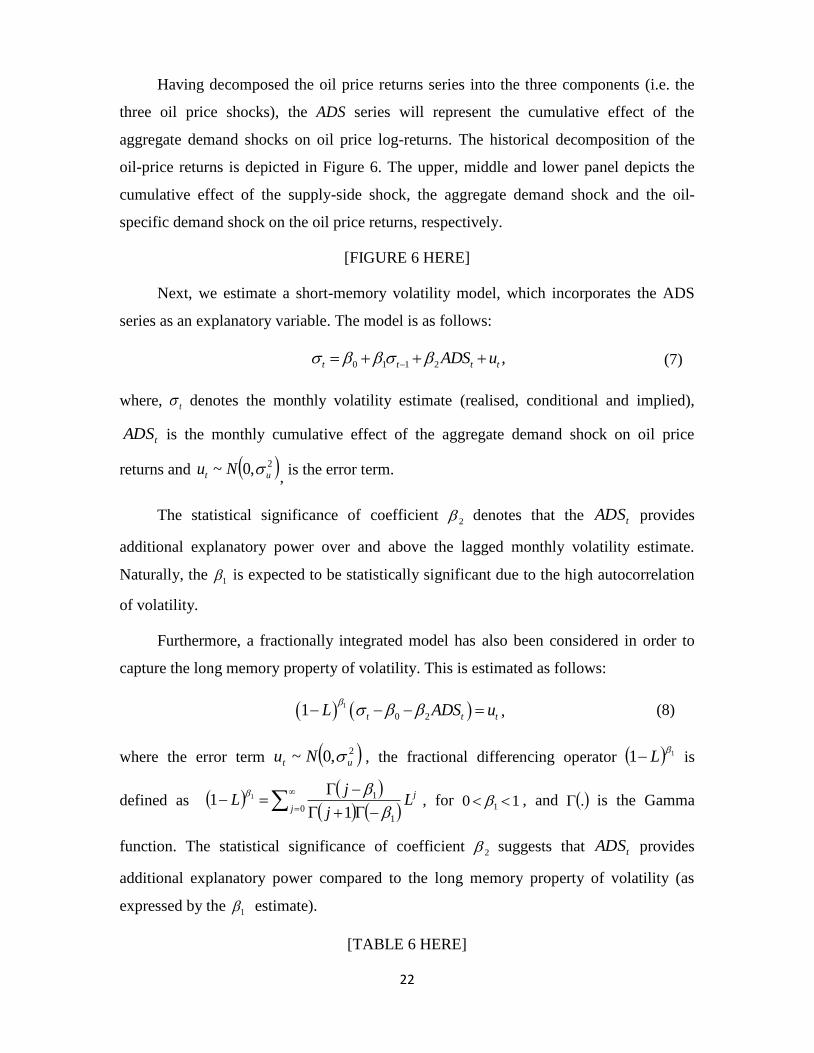
Next, we estimate a short-memory volatility model, which incorporates the ADS

series as an explanatory variable. The model is as follows:

0 1 1 2 ,t t t tADS u (7)

where, t denotes the monthly volatility estimate (realised, conditional and implied),

tADS is the monthly cumulative effect of the aggregate demand shock on oil price

returns and 2,0~ ut Nu , is the error term.

The statistical significance of coefficient 2 denotes that the tADS provides

additional explanatory power over and above the lagged monthly volatility estimate.

Naturally, the 1 is expected to be statistically significant due to the high autocorrelation

of volatility.

Furthermore, a fractionally integrated model has also been considered in order to

capture the long memory property of volatility. This is estimated as follows:

1

0 21 t t tL ADS u , (8)

where the error term 2,0~ ut Nu , the fractional differencing operator 11

L is

defined as

01

1

11 1

j

jLj

jL

, for 10 1 , and . is the Gamma

function. The statistical significance of coefficient 2 suggests that tADS provides

additional explanatory power compared to the long memory property of volatility (as

expressed by the 1 estimate).

[TABLE 6 HERE]

23

[TABLE 7 HERE]

The estimation results, summarised in Tables 6 and 7, indicate that the ADS

exercises a negative and significant effect on stock market volatility. The results are

qualitatively similar for the three volatility measures and for both the aggregate stock

market and industrial sector indices. In particular, a positive aggregate demand shock

causes a reduction in stock market volatility, which confirms the findings of the SVAR

model. The results are, thus, of particular importance as they could facilitate traders,

investors, researchers or policy makers, should they need to forecast stock market

volatility, price derivatives, manage risk and formulate regulation.

6. Concluding remarks

This study examines the effects of three oil prices shocks (i.e., supply-side shock,

aggregate demand shock and oil specific demand shock) on stock market volatility using

a Structural VAR framework. We consider two volatility measures, namely the

conditional volatility and the realised volatility, which measure current stock market

volatility. We also examine the effects of oil price shocks on implied volatility which is a

forward-looking volatility measure.

We conclude that supply-side and oil specific demand shocks do not affect

volatility, whereas, aggregate demand shocks influence volatility at a significant level.

This finding holds for both the current-looking volatility and the implied volatility

measures of aggregate stock market and industrial sector indices. Furthermore, the two

volatility models (short- and long-memory models) verify the SVAR results, suggesting

that the effect of the aggregate demand oil price shocks on volatility is negative and

significant for all indices and all measures. The findings of the study are essential in

pricing financial derivatives, selecting portfolios, measuring and managing investment

risk. Investors, risk managers, even policy makers of central banks and capital market

commissions will find the outcomes of the study useful in handling market's uncertainty

in relation with the state of the oil price shocks. For example, supervisors of financial

institutions must hold capital based on its internal model’s estimates of Value-at-Risk.

The Value-at-Risk internal model can take into consideration the interrelation between oil

price shocks and stock market volatility. The Basel Committee, in order to strengthen

24

bank capital requirements and introduce enhanced regulatory requirements on bank

liquidity, may take advantage of the ability to model the relationship between aggregate

demand oil price shocks and volatility of European stock markets.

It is essential that further studies will distinguish such effects for oil-importing

and oil-exporting countries and conditional correlation models can be used to identify the

aforementioned relationships in a time-varying environment. Finally, following Andersen

et al. (2005), an interesting question underpinning this research is whether and, if so, how

the betas of European stock market sectors respond to different oil price shocks.

25

References

Andersen, T., Bollerslev, T., Diebold, F.X. and Ebens, H. (2001). The

distribution of stock return volatility. Journal of Financial Economics, 61, 43-76.

Andersen, T., Bollerslev, T., Diebold, F.X. and Labys, P. (2003). Modeling and

forecasting realized volatility. Econometrica, 71, 529-626.

Andersen, T., Bollerslev, T. and Meddahi, N. (2005). Correcting the errors:

Volatility forecast evaluation using high-frequency data and realized volatilities.

Econometrica, 73(1), 279-296.

Andersen, T., Bollerslev, T., Diebold, F.X. and Wu, J. (2005). A framework for

exploring the macroeconomic determinants of systematic risk. American Economic

Review Papers and Proceedings, 95, 398-404.

Apergis, N. and Miller, S.M. (2009). Do structural oil - market shocks affect

stock prices? Energy Economics, 31(4), 569-575.

Arouri, M.E.H. (2011). Does crude oil move stock markets in Europe? A sectoral

investigation. Economic Modelling, 28, 1716-1725.

Arouri, M.E.H. and Nguyen, D.K. (2010). Oil prices, stock markets and

portfolio investment: Evidence from sector analysis in Europe over the last decade.

Energy Policy, 38(8), 4528-4539.

Arouri, M.E.H., Jouini, J. and Nguyen D.K. (2011). Volatility spillovers

between oil prices and stock sector returns: Implications for portfolio management.

Journal of International Money and Finance, 30(7), 1387-1405.

Arouri, M.E.H., Jouini, J. and Nguyen D.K. (2012). On the impacts of oil price

fluctuations on European equity markets: Volatility spillover and hedging effectiveness.

Energy Economics, 34, 611-617.

Arouri, M.E.H. and Rault, C. (2011). On the influence of oil prices on stock

markets: Evidence from panel analysis in GCC countries. International Journal of

Finance and Economics, in press, DOI: 10.1002/ijfe.443.

Barndorff-Nielsen, O.E. and Shephard, N. (2002). Econometric analysis of

realised volatility and its use in estimating stochastic volatility models, Journal of the

Royal Statistical Society, Series B, 64, 253–280.

Barsky, R. and Kilian, L. (2004). Oil and the macroeconomy since the 1970s.

Journal of Economic Perspectives, 18, 115-134.

26

Basher, S.A., Haug, A.A. and Sadorsky, P. (2012). Oil prices, exchange rates

and emerging stock markets. Energy Economics, 34, 227-240.

Baum, C.F., Caglaynan, M. and Talavera, O. (2010). On the sensitivity of

firms’ investment to cash flow and uncertainty. Oxford Economic Papers, 62, 286-306.

Baumeister, C. and Peersman, G. (2012). Time-varying effects of oil supply

shocks on the US economy. Bank of Canada Working Paper Series, WP2012-02.

Becker, R., Clements, A.E. and White, S.I. (2007). Does implied volatility

provide any information beyond that captured in model-based volatility forecasts?

Journal of Banking and Finance, 31, 2535-2549.

Bernanke, B.S. (1983). Irreversibility, uncertainty, and cyclical investment.

Quarterly Journal of Economics, 98, 85-106

Bjornland, C.H. (2009). Oil price shocks and stock market booms in an oil

exporting country. Scottish Journal of Political Economy, 2(5), 232-254.

Bjornland, C.H. and Leitemo, K. (2009). Identifying the interdependence

between US monetary policy and the stock market. Journal of Monetary Economics, 56,

275-282.

Blair, B.J., Poon, S-H and Taylor S.J. (2001). Forecasting S&P100 volatility:

The incremental information content of implied volatilities and high-frequency index

returns. Journal of Econometrics, 105, 5-26.

Bloom, N. (2009). The impact of uncertainty shocks. Econometrica, 77, 623-685.

Bollerslev, T., Chou, R. and Kroner, K.F. (1992). ARCH modeling in finance:

A review of the theory and empirical evidence. Journal of Econometrics, 52, 5-59.

Burbidge, J. & Harrison, A. (1985). A historical decomposition of the great

depression to determine the role of money. Journal of Monetary Economics, 16(1), 45-

54.

Chen, S.S. (2009). Do higher oil prices push the stock market into bear territory?

Energy Economics, 32(2), 490-495.

Chiou, J-S. and Lee, Y-H. (2009). Jump dynamics and volatility: Oil and the

stock markets. Energy, 34, 788–796.

Christensen, B.J. and Prabhala, N.R. (1998). The Relation between implied and

realised volatility. Journal of Financial Economics, 50, 125-150.

27

Corrado, C. and Truong, C. (2007). Forecasting stock index volatility:

comparing implied volatility and the intraday high-low price range. Journal of Financial

Research, XXX(2), 201-215.

Cong, R.G., Wei, Y.M., Jiao, J.L. and Fan, Y. (2008). Relationships between

oil price shocks and stock market: An empirical analysis from China. Energy Policy, 36,

3544-3553.

Day, T.E. and Lewis, C.M. (1992). Stock market volatility and the information

content of stock index options. Journal of Econometrics, 52, 267-287.

Ding, Z., Granger, C.W.J. and Engle, R.F. (1993). A long memory property of

stock market returns and a new model. Journal of Empirical Finance, 1, 83-106.

Driesprong, G., Jacobsen, B. and Maat, B. (2008). Striking oil: Another puzzle?

Journal of Financial Economics, 89(2), 307-327.

Elder, J. and Serletis, A. (2011). Oil price uncertainty. Journal of Money, Credit

and Banking, 42, 1137-1159.

Engle, R.F. (2002). New frontiers for ARCH models. Journal of Applied

Econometrics, 17, 425-446.

Filis, G. (2010). Macro economy, stock market and oil prices: Do meaningful

relationships exist among their cyclical fluctuations? Energy Economics, 32(4), 877-886.

Filis, G., Degiannakis, S. and Floros, C. 2011. Dynamic correlation between

stock market and oil prices: The case of oil-importing and oil-exporting countries.

International Review of Financial Analysis, 20(3), 152-164.

Fleming, J. (1998). The quality of market volatility forecast implied by S&P 100

index option prices. Journal of Empirical Finance, 5, 317-345.

Gjerde, O. and Sættem, F. (1999). Causal relations among stock returns and

macroeconomic variables in a small, open economy. Journal of International Financial

Markets, Institutions and Money, 9, 61–74.

Hamilton, J.D. (2009a). Understanding crude oil prices. Energy Journal, 30,

179-206.

Hamilton, J.D. (2009b). Causes and consequences of the oil shock of 2007-08.

Brookings Papers on Economic Activity, Spring 2009, 215-261.

Haung, D.R., Masulis, R.W. and Stoll, H. (1996). Energy shocks and financial

markets. Journal of Futures Markets, 16(1), 1-27.

28

Henriques, I. and Sadorsky, P. (2011). The effect of oil price volatility on

strategic investment. Energy Economics, 33, 79-87.

Hentschel, L. (1995). All in the family: Nesting symmetric and asymmetric

GARCH models. Journal of Financial Economics, 39, 71-104.

Jammazi, R. and Aloui, C. (2010). Wavelet decomposition and regime shifts:

Assessing the effects of crude oil shocks on stock market returns. Energy Policy, 38(3),

1415-1435.

Jones, M.C. and Kaul, G. (1996). Oil and stock markets. Journal of Finance,

51(2), 463-491.

Kilian, L. (2008). Exogenous oil supply shocks: How big are they and how much

do they matter for the U.S. economy? Review of Economics and Statistics, 90, 216-240.

Kilian, L. (2009). Not all oil price shocks are alike: Disentangling demand and

supply shocks in the crude oil market. American Economic Review, 99(3), 1053–1069.

Kilian, L. and Lewis, L.T. (2011). Does the Fed respond to oil price shocks? The

Economic Journal, 121, 1047–1072.

Kilian, L. and Park, C. (2009). The impact of oil price shocks on the U.S. stock

market. International Economic Review, 50(4), 1267-1287.

Koopman, S., Jungbacker, B. and Hol, E. (2005). Forecasting daily variability

of the S&P100 stock index using historical, realised and implied volatility measurements.

Journal of Empirical Finance, 12, 445–475.

Laurent, S. (2004). Analytical derivatives of the APARCH Model.

Computational Economics, 24, 51-57.

Lescaroux, F. and Mignon, V. (2008). On the influence of oil prices on

economic activity and other macroeconomic and financial variables. OPEC Energy

Review, 32, 343-380.

Lippi, F. and Nobili, A. (2009). Oil and the macroeconomy: A quantitative

structural analysis. Bank of Italy Working Paper Series, No. 704.

Maghyereh, A. (2004). Oil price shocks and emerging stock markets. A

generalized VAR approach. International Journal of Applied Econometrics and

Quantitative Studies, 1(2), 27-40.

Malik, F. and Ewing, B. (2009). Volatility transmission between oil prices and

equity sector returns. International Review of Financial Analysis, 18(3), 95-100.

29

Merton, R.C. (1980). On estimating the expected return on the market: An

explanatory investigation. Journal of Financial Economics, 8, 323-361.

Miller, J.I. and Ratti, R.A. (2009). Crude oil and stock markets: Stability,

instability, and bubbles. Energy Economics, 31(4), 559-568.

Park, J. and Ratti, R.A. (2008). Oil prices and stock markets in the U.S. and 13

European countries. Energy Economics, 30, 2587-2608.

Pindyck, R.S. (1991). Irreversibility, uncertainty, and investment. Journal of

Economic Literature, 29, 1110-1148.

Rahman, S. and Serletis, A. (2011). The asymmetric effects of oil price shocks.

Macroeconomic Dynamics, 15, 437-471.

Ratti, R.A., Seol, Y. and Yoon, K.H. (2011). Relative energy price and

investment by European firms. Energy Economics, 33, 721-731.

Sadorsky, P. (1999). Oil price shocks and stock market activity. Energy

Economics, 21, 449-469.

Sadorsky, P. (2011). Correlations and volatility spillovers between oil prices and

the stock prices of clean energy and technology companies. Energy Economics, in press,

DOI:10.1016/j.eneco.2011.03.006

Scholtens, B. and Yurtsever, C. (2012). Oil price shocks and European

industries. Energy Economics, in press, doi:10.1016/j.eneco.2011.10.012.

Vo, M. (2011). Oil and stock market volatility: A multivariate stochastic volatility

perspective. Energy Economics, 33(5), 956-965.

Xekalaki, E. and Degiannakis, S. (2010). ARCH models for financial

applications. New York: Wiley.

30

Appendix

Figures

Figure 1: Volatility measures of the Eurostoxx 50 index, oil production growth rate, global economic

activity and oil price returns.

Volatility Measures of the Eurostoxx 50

Oil Production Growth Rate

(PROD)

Global Economic Activity

(GEA)

Oil Price Returns

(OP)

31

Figure 2: Impulse Responses of RV_STOXX50 and CV_STOXX50.

Note: Shock 1 refers to the supply-side shock (PROD), Shock 2 refers to the aggregate demand shock

(GEA), Shock 3 refers to the oil specific demand shock (OP) and Shock 4 refers to the volatility shock

(VOL).

-.08

-.04

.00

.04

.08

.12

2 4 6 8 10 12 14 16

Response of RV_STOXX50 to Shock1

-.08

-.04

.00

.04

.08

.12

2 4 6 8 10 12 14 16


-.08

-.04

.00

.04

.08

.12

2 4 6 8 10 12 14 16


-.08

-.04

.00

.04

.08

.12

2 4 6 8 10 12 14 16


Response to Structural One S.D. Innovations ± 2 S.E.

-.08

-.04

.00

.04

.08

2 4 6 8 10 12 14 16

Response of CV_STOXX50 to Shock1

-.08

-.04

.00

.04

.08

2 4 6 8 10 12 14 16


-.08

-.04

.00

.04

.08

2 4 6 8 10 12 14 16


-.08

-.04

.00

.04

.08

2 4 6 8 10 12 14 16


32

Figure 3: Impulse Responses of the industrial sectors’ conditional volatilities.

Note: Shock 1 refers to the supply-side shock (PROD), Shock 2 refers to the aggregate demand shock (GEA), Shock 3

refers to the oil specific demand shock (OP) and Shock 4 refers to the volatility shock (VOL). The order of the

industrial indices are as follows: Consumer Goods, Financials, Health, Industrials, Basic Material, Oil&Gas, Retail,

Technology, Telecommunications, Utilities.

-.08

-.04

.00

.04

.08

2 4 6 8 10 12 14 16

Response of CV_CONS to Shock1

-.08

-.04

.00

.04

.08

2 4 6 8 10 12 14 16


-.08

-.04

.00

.04

.08

2 4 6 8 10 12 14 16


-.08

-.04

.00

.04

.08

2 4 6 8 10 12 14 16


-.10

-.05

.00

.05

.10

2 4 6 8 10 12 14 16

Response of CV_FINS to Shock1

-.10

-.05

.00

.05

.10

2 4 6 8 10 12 14 16


-.10

-.05

.00

.05

.10

2 4 6 8 10 12 14 16


-.10

-.05

.00

.05

.10

2 4 6 8 10 12 14 16


-.04

-.02

.00

.02

.04

.06

2 4 6 8 10 12 14 16

Response of CV_HEALTH to Shock1

-.04

-.02

.00

.02

.04

.06

2 4 6 8 10 12 14 16


-.04

-.02

.00

.02

.04

.06

2 4 6 8 10 12 14 16


-.04

-.02

.00

.02

.04

.06

2 4 6 8 10 12 14 16


-.08

-.04

.00

.04

.08

2 4 6 8 10 12 14 16

Response of CV_INDS to Shock1

-.08

-.04

.00

.04

.08

2 4 6 8 10 12 14 16


-.08

-.04

.00

.04

.08

2 4 6 8 10 12 14 16


-.08

-.04

.00

.04

.08

2 4 6 8 10 12 14 16


-.08

-.04

.00

.04

.08

2 4 6 8 10 12 14 16

Response of CV_MAT to Shock1

-.08

-.04

.00

.04

.08

2 4 6 8 10 12 14 16


-.08

-.04

.00

.04

.08

2 4 6 8 10 12 14 16


-.08

-.04

.00

.04

.08

2 4 6 8 10 12 14 16


-.08

-.04

.00

.04

.08

2 4 6 8 10 12 14 16

Response of CV_OILGAS to Shock1

-.08

-.04

.00

.04

.08

2 4 6 8 10 12 14 16


-.08

-.04

.00

.04

.08

2 4 6 8 10 12 14 16


-.08

-.04

.00

.04

.08

2 4 6 8 10 12 14 16


-.06

-.04

-.02

.00

.02

.04

.06

2 4 6 8 10 12 14 16

Response of CV_RETAIL to Shock1

-.06

-.04

-.02

.00

.02

.04

.06

2 4 6 8 10 12 14 16


-.06

-.04

-.02

.00

.02

.04

.06

2 4 6 8 10 12 14 16


-.06

-.04

-.02

.00

.02

.04

.06

2 4 6 8 10 12 14 16


-.08

-.04

.00

.04

.08

2 4 6 8 10 12 14 16

Response of CV_TECH to Shock1

-.08

-.04

.00

.04

.08

2 4 6 8 10 12 14 16


-.08

-.04

.00

.04

.08

2 4 6 8 10 12 14 16


-.08

-.04

.00

.04

.08

2 4 6 8 10 12 14 16


-.08

-.04

.00

.04

.08

2 4 6 8 10 12 14 16

Response of CV_TEL to Shock1

-.08

-.04

.00

.04

.08

2 4 6 8 10 12 14 16


-.08

-.04

.00

.04

.08

2 4 6 8 10 12 14 16


-.08

-.04

.00

.04

.08

2 4 6 8 10 12 14 16


-.08

-.04

.00

.04

.08

2 4 6 8 10 12 14 16

Response of CV_UTIL to Shock1

-.08

-.04

.00

.04

.08

2 4 6 8 10 12 14 16


-.08

-.04

.00

.04

.08

2 4 6 8 10 12 14 16


-.08

-.04

.00

.04

.08

2 4 6 8 10 12 14 16


33

Figure 4: Impulse Responses of the industrial sectors’ realised volatilities.

Note: Shock 1 refers to the supply-side shock (PROD), Shock 2 refers to the aggregate demand shock (GEA), Shock 3

refers to the oil specific demand shock (OP) and Shock 4 refers to the volatility shock (VOL). The order of the

industrial indices are as follows: Consumer Goods, Financials, Health, Industrials, Basic Material, Oil&Gas, Retail,

Technology, Telecommunications, Utilities.

-.08

-.04

.00

.04

.08

.12

2 4 6 8 10 12 14 16

Response of RV_CONS to Shock1

-.08

-.04

.00

.04

.08

.12

2 4 6 8 10 12 14 16


-.08

-.04

.00

.04

.08

.12

2 4 6 8 10 12 14 16


-.08

-.04

.00

.04

.08

.12

2 4 6 8 10 12 14 16


-.10

-.05

.00

.05

.10

.15

2 4 6 8 10 12 14 16

Response of RV_FINS to Shock1

-.10

-.05

.00

.05

.10

.15

2 4 6 8 10 12 14 16


-.10

-.05

.00

.05

.10

.15

2 4 6 8 10 12 14 16


-.10

-.05

.00

.05

.10

.15

2 4 6 8 10 12 14 16


-.08

-.04

.00

.04

.08

2 4 6 8 10 12 14 16

Response of RV_HEALTH to Shock1

-.08

-.04

.00

.04

.08

2 4 6 8 10 12 14 16


-.08

-.04

.00

.04

.08

2 4 6 8 10 12 14 16


-.08

-.04

.00

.04

.08

2 4 6 8 10 12 14 16


-.08

-.04

.00

.04

.08

.12

2 4 6 8 10 12 14 16

Response of RV_INDS to Shock1

-.08

-.04

.00

.04

.08

.12

2 4 6 8 10 12 14 16


-.08

-.04

.00

.04

.08

.12

2 4 6 8 10 12 14 16


-.08

-.04

.00

.04

.08

.12

2 4 6 8 10 12 14 16


-.10

-.05

.00

.05

.10

2 4 6 8 10 12 14 16

Response of RV_MAT to Shock1

-.10

-.05

.00

.05

.10

2 4 6 8 10 12 14 16


-.10

-.05

.00

.05

.10

2 4 6 8 10 12 14 16


-.10

-.05

.00

.05

.10

2 4 6 8 10 12 14 16


-.10

-.05

.00

.05

.10

2 4 6 8 10 12 14 16

Response of RV_OILGAS to Shock1

-.10

-.05

.00

.05

.10

2 4 6 8 10 12 14 16


-.10

-.05

.00

.05

.10

2 4 6 8 10 12 14 16


-.10

-.05

.00

.05

.10

2 4 6 8 10 12 14 16


-.050

-.025

.000

.025

.050

.075

.100

2 4 6 8 10 12 14 16

Response of RV_RETAIL to Shock1

-.050

-.025

.000

.025

.050

.075

.100

2 4 6 8 10 12 14 16


-.050

-.025

.000

.025

.050

.075

.100

2 4 6 8 10 12 14 16


-.050

-.025

.000

.025

.050

.075

.100

2 4 6 8 10 12 14 16


-.08

-.04

.00

.04

.08

.12

2 4 6 8 10 12 14 16

Response of RV_TECH to Shock1

-.08

-.04

.00

.04

.08

.12

2 4 6 8 10 12 14 16


-.08

-.04

.00

.04

.08

.12

2 4 6 8 10 12 14 16


-.08

-.04

.00

.04

.08

.12

2 4 6 8 10 12 14 16


-.08

-.04

.00

.04

.08

.12

2 4 6 8 10 12 14 16

Response of RV_TEL to Shock1

-.08

-.04

.00

.04

.08

.12

2 4 6 8 10 12 14 16


-.08

-.04

.00

.04

.08

.12

2 4 6 8 10 12 14 16


-.08

-.04

.00

.04

.08

.12

2 4 6 8 10 12 14 16


-.08

-.04

.00

.04

.08

.12

2 4 6 8 10 12 14 16

Response of RV_UTIL to Shock1

-.08

-.04

.00

.04

.08

.12

2 4 6 8 10 12 14 16


-.08

-.04

.00

.04

.08

.12

2 4 6 8 10 12 14 16


-.08

-.04

.00

.04

.08

.12

2 4 6 8 10 12 14 16


34

Figure 5: Impulse Responses of VSTOXX.

Note: Shock 1 refers to the supply-side shock (PROD), Shock 2 refers to the aggregate demand shock

(GEA), Shock 3 refers to the oil specific demand shock (OP) and Shock 4 refers to the volatility shock

(VOL).

Figure 6: Historical Decomposition of Oil Price Returns.

Note: This figure depicts historical decomposition of the oil price returns. The upper (middle, lower) panel

depicts the cumulative effect of the supply-side shock (PROD), the aggregate demand shock (GEA) and the

oil-specific demand shock (OP).

-.08

-.04

.00

.04

.08

2 4 6 8 10 12 14 16

Response of VSTOXX to Shock1

-.08

-.04

.00

.04

.08

2 4 6 8 10 12 14 16


-.08

-.04

.00

.04

.08

2 4 6 8 10 12 14 16


-.08

-.04

.00

.04

.08

2 4 6 8 10 12 14 16


Response to Structural One S.D. Innovations ± 2 S.E.

Effect of PROD

1999 2000 2001 2002 2003 2004 2005 2006 2007 2008 2009 2010

-0.3

-0.1

0.1

0.3

Effect of GEA

1999 2000 2001 2002 2003 2004 2005 2006 2007 2008 2009 2010

-0.3

-0.1

0.1

0.3

Effect of OP

1999 2000 2001 2002 2003 2004 2005 2006 2007 2008 2009 2010

-0.3

-0.1

0.1

0.3

35

Tables

Table 1: Descriptive statistics of RV_STOXX50, CV_STOXX50, VSTOXX, PROD, GEA

and OP.

RV_STOXX50 CV_STOXX50 VSTOXX PROD GEA OP

Mean 23.41% 23.94% 30.48% 0.06% 8.89% 1.49%

Maximum 83.55% 85.70% 82.72% 2.89% 54.30% 26.75%

Minimum 9.38% 10.61% 15.45% -2.44% -51.30% -32.11%

Std. Dev. 13.20% 11.57% 12.38% 0.91% 26.19% 11.98%

Skewness 2.038 2.170 1.448 0.045 -0.259 -0.643

Kurtosis 8.013 9.510 5.466 3.813 2.099 3.248

Table 2: Variance Decomposition – Current-looking volatility measures.

Volatility Measure

Time Period

PROD

GEA

OP

VOL

CV_STOXX50

1

0.318

13.389

4.334

81.959

3

0.873

22.524

3.613

72.990

6

1.238

30.827

4.793

63.141

12

1.370

30.799

5.035

62.796

18

1.417

30.720

5.004

62.859

24

1.469

30.872

4.988

62.671

RV_STOXX50

1

0.835

6.425

2.197

90.542

3

0.924

13.082

3.188

82.806

6

1.459

16.996

3.773

77.771

12

1.801

17.057

4.092

77.050

18

1.816

17.175

4.087

76.921

24

1.837

17.257

4.088

76.818

36

Table 3: Variance Decomposition – Industrial sectors – Conditional Volatility.

Industrial sector

Time

Period

PROD

GEA

OP

VOL

CV_CONSUMER

1

0.04105

18.0963

3.97052

77.8922

3

1.03125

32.4045

3.61692

62.9473

6

1.20629

40.2086

4.61741

53.9677

12

1.31018

39.8584

4.77912

54.0524

18

1.45074

39.705

4.73764

54.1066

24

1.56107

39.8382

4.73764

53.8631

CV_FINANCIALS

1

0.27831

10.7337

3.15151

85.8365

3

0.95159

18.1702

3.0277

77.8506

6

1.04201

24.2855

4.62298

70.0495

12

1.12005

23.5867

5.06639

70.2269

18

1.28088

23.6219

4.96934

70.1279

24

1.45144

24.0705

4.90703

69.571

CV_HEALTH

1

1.22322

16.777

4.07704

77.9228

3

1.37515

27.3975

3.09657

68.1308

6

3.04791

31.2977

3.5477

62.1067

12

3.36313

32.0552

3.93312

60.6485

18

3.37275

32.0556

3.94709

60.6246

24

3.3727

32.0558

3.94708

60.6244

CV_INDUSTRIAL

1

0.62348

15.027

5.3342

79.0153

3

1.23732

22.6861

3.8773

72.1993

6

1.157

26.4947

4.46518

67.8831

12

1.1737

25.263

4.48806

69.0753

18

1.36132

25.3829

4.3681

68.8877

24

1.51265

26.0653

4.3078

68.1142

CV_MATERIALS

1

0.28495

17.943

3.92154

77.8505

3

0.86182

30.029

3.80046

65.3087

6

1.25674

35.6899

5.0614

57.992

12

1.33202

34.8198

5.46355

58.3846

18

1.49483

34.9077

5.36156

58.2359

24

1.65423

35.1899

5.32808

57.8278

CV_OIL&GAS

1

0.52025

23.7492

7.23176

68.4988

3

1.18125

36.7335

7.06484

55.0204

6

1.8483

43.4956

7.65192

47.0042

37

Table 3 (continued)

12

2.09462

42.8753

8.00695

47.0232

18

2.15193

42.8498

7.92557

47.0727

24

2.22034

43.0125

7.89596

46.8712

CV_RETAIL

1

0.75457

13.1533

1.05536

85.0368

3

1.64064

22.1003

0.57449

75.6846

6

1.69859

25.0061

0.63189

72.6634

12

1.66014

24.5233

0.62673

73.1899

18

1.69588

24.4783

0.64802

73.1778

24

1.71982

24.5356

0.66437

73.0802

CV_TECHNOLO

GY

1

1.68888

14.4082

4.21653

79.6864

3

1.71655

22.0778

2.5365

73.6691

6

1.24896

31.1126

2.33212

65.3063

12

1.07055

32.9725

2.21435

63.7426

18

1.03425

33.0633

2.18002

63.7225

24

1.02698

33.0428

2.16952

63.7607

CV_TELECOMM

UNICATIONS

1

0.3086

17.7102

2.64539

79.3358

3

1.97908

29.0347

2.64088

66.3454

6

1.60388

33.5286

2.07586

62.7917

12

1.48391

34.4417

1.84691

62.2275

18

1.45568

34.7526

1.803

61.9887

24

1.44764

34.844

1.79333

61.915

CV_UTILITIES

1

0.54323

19.335

3.12126

77.0005

3

0.89482

31.272

4.73463

63.0986

6

1.46511

34.4648

6.29527

57.7748

12

1.58069

34.1397

6.5359

57.7437

18

1.76665

34.5144

6.45937

57.2596

24 1.90042 34.7715 6.43394 56.8942

38

Table 4: Variance Decomposition – Industrial sectors – Realised Volatility.

Industrial sector

Time

Period

PROD

GEA

OP

VOL

RV_CONSUMER

1

0.04565

20.672

2.29441

76.9879

3

1.33782

33.8628

2.41952

62.3798

6

1.97986

38.3806

2.9936

56.646

12

2.40929

38.1632

2.98492

56.4426

18

2.54313

38.2369

3.0039

56.2161

24

2.60908

38.301

3.02181

56.0681

RV_FINANCIALS

1

0.49498

4.42609

3.16536

91.9136

3

1.13097

8.41176

3.09396

87.3633

6

1.05986

12.1545

4.0093

82.7764

12

1.21465

11.8632

4.33898

82.5832

18

1.34222

12.4592

4.27659

81.922

24

1.476

12.9796

4.2451

81.2993

RV_HEALTH

1

1.58446

12.0845

2.86428

83.4668

3

1.02134

20.188

2.58358

76.2071

6

2.97149

21.4084

3.26278

72.3573

12

3.35235

21.8914

3.58715

71.1692

18

3.37727

21.9606

3.59941

71.0627

24

3.38228

21.9842

3.60085

71.0327

RV_INDUSTRIAL

1

0.68778

9.15656

5.62758

84.5281

3

0.94328

14.5157

4.89125

79.6498

6

0.85716

14.8578

5.05265

79.2324

12

0.91703

14.2116

4.97917

79.8922

18

1.06814

14.7076

4.89914

79.3251

24

1.18099

15.1543

4.86943

78.7953

RV_MATERIALS

1

0.15249

12.3487

4.84597

82.6528

3

0.82122

20.5373

4.55745

74.0841

6

2.01679

22.2354

5.48122

70.2666

12

2.2017

21.6978

5.83422

70.2663

18

2.30592

22.2116

5.75469

69.7278

24

2.41735

22.5427

5.72654

69.3134

RV_OIL&GAS

1

0.231

11.3947

3.78719

84.5871

3

1.50748

22.8078

4.32821

71.3565

6

2.45933

25.7115

4.54275

67.2864

39

Table 4 (continued)

12

2.8764

25.2687

4.58549

67.2694

18

2.90528

25.5085

4.57743

67.0088

24

2.94477

25.7099

4.5898

66.7555

RV_RETAIL

1

1.26258

7.93259

0.64978

90.1551

3

1.69779

14.9768

0.51573

82.8097

6

1.6629

15.3522

0.69026

82.2946

12

1.65921

15.1493

0.71461

82.4769

18

1.67259

15.2114

0.72079

82.3952

24

1.68415

15.2531

0.72898

82.3338

RV_TECHNOLOGY

1

0.32981

10.6097

4.61063

84.4499

3

1.43372

16.6987

2.86743

79.0001

6

1.11957

21.2468

2.26143

75.3722

12

1.13673

23.7168

2.00492

73.1416

18

1.17524

24.7174

1.96134

72.146

24

1.20144

25.0432

1.95172

71.8036

RV_TELECOMMUNI

CATIONS

1

0.53754

10.4097

1.20533

87.8475

3

1.90242

17.0721

1.5078

79.5176

6

1.54601

19.8576

1.88056

76.7159

12

1.63096

20.404

2.02587

75.9391

18

1.66546

21.0169

1.99595

75.3217

24

1.70046

21.238

1.98843

75.0731

RV_UTILITIES

1

0.52452

10.4482

0.97392

88.0534

3

0.72767

18.247

4.24764

76.7777

6

1.25227

17.9609

4.997

75.7898

12

1.4318

17.9779

5.20114

75.3892

18

1.55453

18.4291

5.20351

74.8129

24 1.63201 18.6198 5.21536 74.5328

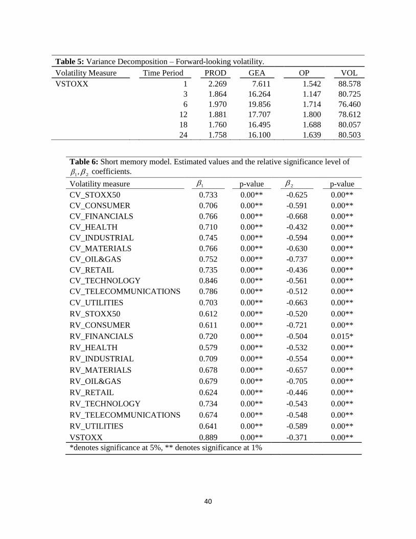
40

Table 5: Variance Decomposition – Forward-looking volatility.

Volatility Measure

Time Period

PROD

GEA

OP

VOL

VSTOXX

1

2.269

7.611

1.542

88.578

3

1.864

16.264

1.147

80.725

6

1.970

19.856

1.714

76.460

12

1.881

17.707

1.800

78.612

18

1.760

16.495

1.688

80.057

24 1.758 16.100 1.639 80.503

Table 6: Short memory model. Estimated values and the relative significance level of

1 ,2 coefficients.

Volatility measure

p-value

p-value

CV_STOXX50 0.733

0.00**

-0.625

0.00**

CV_CONSUMER 0.706

0.00**

-0.591

0.00**

CV_FINANCIALS 0.766

0.00**

-0.668

0.00**

CV_HEALTH 0.710

0.00**

-0.432

0.00**

CV_INDUSTRIAL 0.745

0.00**

-0.594

0.00**

CV_MATERIALS 0.766

0.00**

-0.630

0.00**

CV_OIL&GAS 0.752

0.00**

-0.737

0.00**

CV_RETAIL 0.735

0.00**

-0.436

0.00**

CV_TECHNOLOGY 0.846

0.00**

-0.561

0.00**

CV_TELECOMMUNICATIONS 0.786

0.00**

-0.512

0.00**

CV_UTILITIES 0.703

0.00**

-0.663

0.00**

RV_STOXX50 0.612

0.00**

-0.520

0.00**

RV_CONSUMER 0.611

0.00**

-0.721

0.00**

RV_FINANCIALS 0.720

0.00**

-0.504

0.015*

RV_HEALTH 0.579

0.00**

-0.532

0.00**

RV_INDUSTRIAL 0.709

0.00**

-0.554

0.00**

RV_MATERIALS 0.678

0.00**

-0.657

0.00**

RV_OIL&GAS 0.679

0.00**

-0.705

0.00**

RV_RETAIL 0.624

0.00**

-0.446

0.00**

RV_TECHNOLOGY 0.734

0.00**

-0.543

0.00**

RV_TELECOMMUNICATIONS 0.674

0.00**

-0.548

0.00**

RV_UTILITIES 0.641

0.00**

-0.589

0.00**

VSTOXX 0.889

0.00**

-0.371

0.00**

*denotes significance at 5%, ** denotes significance at 1%

1 2

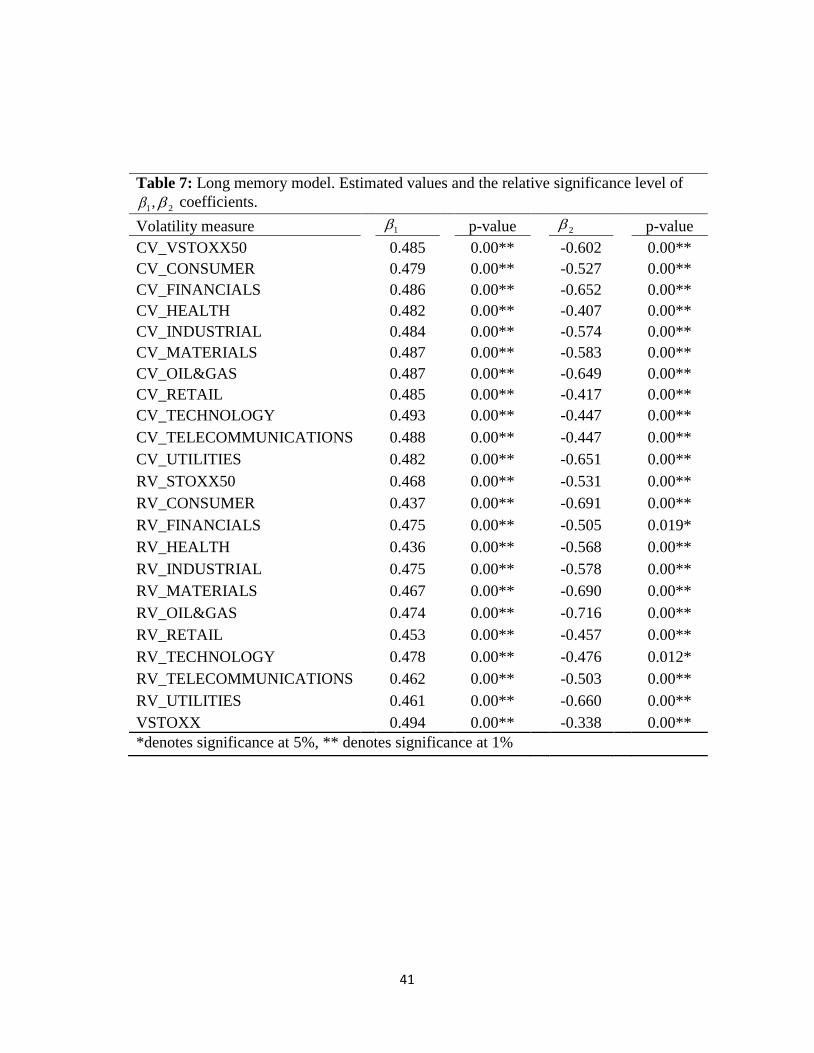
41

Table 7: Long memory model. Estimated values and the relative significance level of

1 ,2 coefficients.

Volatility measure

p-value

p-value

CV_VSTOXX50 0.485

0.00**

-0.602

0.00**

CV_CONSUMER 0.479

0.00**

-0.527

0.00**

CV_FINANCIALS 0.486

0.00**

-0.652

0.00**

CV_HEALTH 0.482

0.00**

-0.407

0.00**

CV_INDUSTRIAL 0.484

0.00**

-0.574

0.00**

CV_MATERIALS 0.487

0.00**

-0.583

0.00**

CV_OIL&GAS 0.487

0.00**

-0.649

0.00**

CV_RETAIL 0.485

0.00**

-0.417

0.00**

CV_TECHNOLOGY 0.493

0.00**

-0.447

0.00**

CV_TELECOMMUNICATIONS 0.488

0.00**

-0.447

0.00**

CV_UTILITIES 0.482

0.00**

-0.651

0.00**

RV_STOXX50 0.468

0.00**

-0.531

0.00**

RV_CONSUMER 0.437

0.00**

-0.691

0.00**

RV_FINANCIALS 0.475

0.00**

-0.505

0.019*

RV_HEALTH 0.436

0.00**

-0.568

0.00**

RV_INDUSTRIAL 0.475

0.00**

-0.578

0.00**

RV_MATERIALS 0.467

0.00**

-0.690

0.00**

RV_OIL&GAS 0.474

0.00**

-0.716

0.00**

RV_RETAIL 0.453

0.00**

-0.457

0.00**

RV_TECHNOLOGY 0.478

0.00**

-0.476

0.012*

RV_TELECOMMUNICATIONS 0.462

0.00**

-0.503

0.00**

RV_UTILITIES 0.461

0.00**

-0.660

0.00**

VSTOXX 0.494

0.00**

-0.338

0.00**

*denotes significance at 5%, ** denotes significance at 1%

1 2

42

BANK OF GREECE WORKING PAPERS

144. Gazopoulou, E. “A note on the effectiveness of price policy on tourist arrivals to Greece”, May 2012.

145. Tagkalakis, A. “The Effects of Financial Crisis on Fiscal Positions”, June 2012.

146. Bakas, D., and E. Papapetrou, “Unemployment in Greece: Evidence from Greek Regions”, June 2012.

147. Angelopoulou, E, H. Balfoussia and H. Gibson, “Building a Financial Conditions Index for the Euro Area and Selected Euro Area Countries: What Does it Tell Us About The Crisis?”, July 2012.

148. Brissimis, S, E. Garganas and S. Hall, “Consumer Credit in an Era of Financial Liberalisation: an Overreaction to Repressed Demand?”, October 2012

149. Dellas, H., and G. Tavlas, “The Road to Ithaca: the Gold Standard, the Euro and the Origins of the Greek Sovereign Debt Crisis”, November 2012.

150. Philippopoulos, A., P. Varthalitis, and V. Vassilatos, “On The Optimal Mix of Fiscal and Monetary Policy Actions”, December 2012.

151. Brissimis, N. S. and P. M. Migiakis, “Inflation Persistence and the Rationality of Inflation Expectations”, January 2013.

152. Tagkalakis, O. A., “Audits and Tax Offenders: Recent Evidence from Greece”, February 2013.

153. Bageri, V., Y. Katsoulacos, and G.Spagnolo, “The Distortive Effects of Antitrust Fines Based on Revenue”, February 2013.

154. Louzis, P. D., “Measuring Return and Volatility Spillovers in Euro Area Financial Markets”, March 2013

155. Louzis, P. D., and A.T. Vouldis,“A Financial Systemic Stress Index for Greece”, March 2013.

156. Nicolitsas, D., “Price Setting Practices in Greece: Evidence From a Small-Scale Firm-Level Survey”, April 2013

157. Bragoudakis, G. Z., S.T. Panagiotou and H. A. Thanopoulou, “Investment Strategy and Greek Shipping Earnings: Exploring The Pre & Post "Ordering-Frenzy" Period”, April 2013.

158. Kasselaki, Th. M. and O, Tagkalakis, “Financial Soundness Indicators and Financial Crisis Episodes”, April 2013.

159. Bardakas, C.I., “The Asymmetric Effect of Income on Import Demand in Greece”, May 2013.

160. Chassamboulli, A., and T. Palivos, “The Impact of Immigration on the Employment and Wages of Native Workers”, June 2013.

Oil price shocks and stock market volatility

Documents

Transcript of Oil price shocks and stock market volatility