DEWEK 2015 – 12th German Wind Energy Conference

1/4

Representativeness of short-term wind profile measurements with remote sensing devices and consideration of seasonal effects

Annette Westerhellweg, Daniel Fabian, Jan Raabe

UL International GmbH - DEWI, Wilhelmshaven, Germany, a.westerhellweg@dewi.de

Abstract

Especially in Germany hub heights greatly exceeding 100 m are more and more common for new planned wind farms. On the other hand reference wind turbines (wt) often have a significantly lower hub height and therefore the estimation of the vertical wind profile has high uncertainties. Short term measurements by remote sensing devices (RSD) provide a way to assess and verify the wind profile between the hub height of the reference wt or a parallel mast measurement and the planned hub height.

In general, there are strong daily and seasonal variations of the vertical wind profile. Therefore the measured wind profile of a short-term measurement campaign cannot be directly transferred to long-term conditions. The representativeness of the measured wind profile has to be validated and in case that it is not representative the wind profile has to be corrected. DEWI has developed and uses two different methods for the correction of seasonal effects, the seasonal correction based on the correlation with the solar altitude and the wind shear correlation [1]. The seasonal correction method has been further developed to include the dependency on the atmospheric stability.

A sensitivity study of the chosen period of a short term wind profile measurement on the predicted wind speed in hub height has been performed. Finally the results of applied corrections of the wind profile were compared.

1. Data Base

Seasonal effects have been tested on six remote sensing measurements in Germany which had a duration of a full year each. A sensitivity study has been conducted for varying input periods. The input periods have been varied in length (of 3 months and 6 months) and season. All sites are flat according to the definition in the IEC 61400-1 [2], but partly located in slightly undulated terrain. The roughness varies from open landscape to forest. In each case the 1-year measurement was subdivided in 3-months and 6-months periods. The wind shear exponent α has been calculated according to the

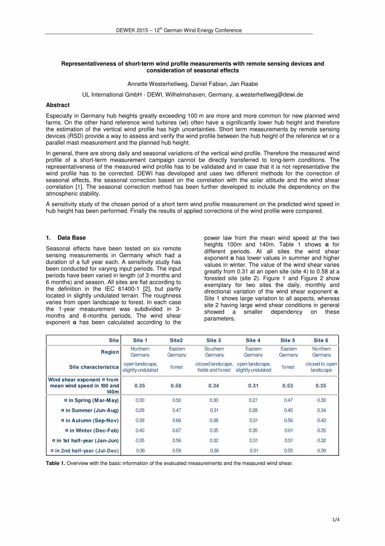
power law from the mean wind speed at the two heights 100m and 140m. Table 1 shows α for different periods. At all sites the wind shear exponent α has lower values in summer and higher values in winter. The value of the wind shear varies greatly from 0.31 at an open site (site 4) to 0.58 at a forested site (site 2). Figure 1 and Figure 2 show exemplary for two sites the daily, monthly and directional variation of the wind shear exponent α. Site 1 shows large variation to all aspects, whereas site 2 having large wind shear conditions in general showed a smaller dependency on these parameters.

Table 1. Overview with the basic information of the evaluated measurements and the measured wind shear.

Site Site 1 Site2 Site 3 Site 4 Site 5 Site 6

RegionNorthern

Germany

Eastern

Germany

Southern

Germany

Eastern

Germany

Eastern

Germany

Northern

Germany

Site characteristicaopen landscape,

slightly undulatedforest

closed landscape,

fields and forest

open landscape,

slightly undulatedforest

closed to open

landscape

Wind shear exponent α from mean wind speed in 100 and

140m

0.35 0.58 0.34 0.31 0.53 0.35

α in Spring (M ar-M ay) 0.30 0.50 0.30 0.27 0.47 0.30

α in Summer (Jun-Aug) 0.29 0.47 0.31 0.28 0.45 0.34

α in Autumn (Sep-Nov) 0.39 0.66 0.38 0.31 0.56 0.42

α in Winter (Dec-Feb) 0.40 0.67 0.35 0.35 0.61 0.35

α in 1st half-year (Jan-Jun) 0.35 0.56 0.32 0.31 0.51 0.32

α in 2nd half-year (Jul-Dec) 0.36 0.59 0.36 0.31 0.55 0.39

DEWEK 2015 – 12th German Wind Energy Conference

2/4

Figure 1. Diurnal, monthly and direction distribution of the wind shear exponent α for site 1.

Figure 2. Diurnal, monthly and direction distribution of the wind shear exponent α for site 2.

2. Dependency of wind shear on atmospheric stability

Two easily assessable parameters for a stability description are the solar altitude and z/L from MERRA [3] data.

MERRA data sets of the temperature, humidity and sensible heat flux have been used to calculate the stability parameter z/L as outlined in [4] with Monin-Obukhov length L and height z. Positive values of z/L indicate stable and negative values of z/L indicate unstable stratification. Under neutral conditions z/L is Zero.

The Monin-Obhukhov length L has been assessed according to [5]:

� � ���

� · � · � · �

� · � · ��

With v* = friction velocity �� · ���� κ = Karman Constant with κ = 0.40 g = gravidity �� · ���� with g = 9.81 Tv = virtual Temperature [K]

cp = specific heat capacity of air �� · ���� · ���� ρ0 = air density at sea level ��� · ���� QH = sensible heat flux �� · ����

with the virtual temperature being calculated from the temperature and specific humidity:

� � � · �1 � 0,61 · #$ with T = temperature [K] q = specific humidity [�� · ����] and with the heat capacity of air calculated by

� � �& · �1 � 0,84 · #$

With cpL = specific heat capacity of dry air �� · ���� ·

���� with cpL = 1004.67

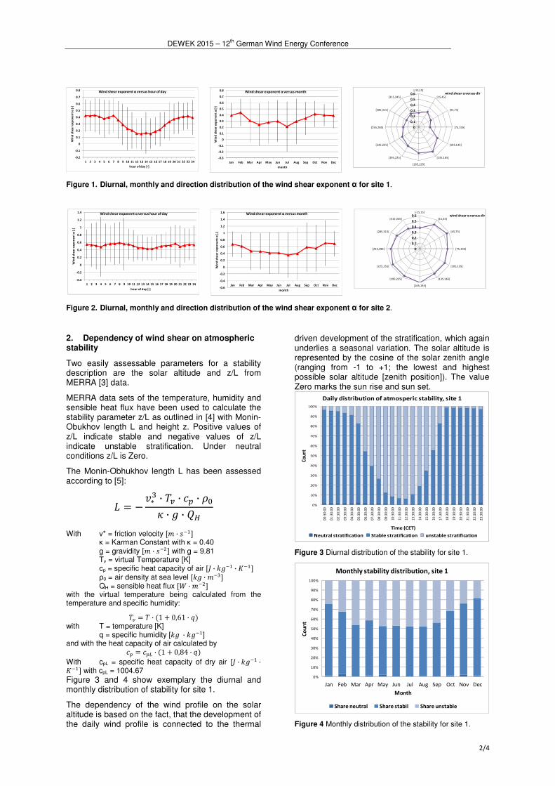
Figure 3 and 4 show exemplary the diurnal and monthly distribution of stability for site 1.

The dependency of the wind profile on the solar altitude is based on the fact, that the development of the daily wind profile is connected to the thermal

driven development of the stratification, which again underlies a seasonal variation. The solar altitude is represented by the cosine of the solar zenith angle (ranging from -1 to +1; the lowest and highest possible solar altitude [zenith position]). The value Zero marks the sun rise and sun set.

Figure 3 Diurnal distribution of the stability for site 1.

Figure 4 Monthly distribution of the stability for site 1.

-0.2

-0.1

0

0.1

0.2

0.3

0.4

0.5

0.6

0.7

0.8

1 2 3 4 5 6 7 8 9 10 11 12 13 14 15 16 17 18 19 20 21 22 23 24

Win

d s

he

ar

exp

on

en

t α

[-]

hour of day [-]

Wind shear exponent α versus hour of day

-0.3

-0.2

-0.1

0

0.1

0.2

0.3

0.4

0.5

0.6

0.7

0.8

Jan Feb Mar Apr May Jun Jul Aug Sep Oct Nov Dec

Win

d s

he

ar

exp

on

en

t α

[-]

month

Wind shear exponent α versus month

0

0.1

0.2

0.3

0.4

0.5

0.6[-15,15[

[15,45[

[45,75[

[75,105[

[105,135[

[135,165[

[165,195[

[195,225[

[225,255[

[255,285[

[285,315[

[315,345[

wind shear α versus dir

-0.4

-0.2

0

0.2

0.4

0.6

0.8

1

1.2

1.4

1 2 3 4 5 6 7 8 9 10 11 12 13 14 15 16 17 18 19 20 21 22 23 24

Win

d s

he

ar

exp

on

en

t α

[-]

hour of day [-]

Wind shear exponent α versus hour of day

-0.6

-0.4

-0.2

0

0.2

0.4

0.6

0.8

1

1.2

1.4

1.6

Jan Feb Mar Apr May Jun Jul Aug Sep Oct Nov Dec

Win

d s

he

ar

exp

on

en

t α

[-]

month

Wind shear exponent α versus month

0

0.1

0.2

0.3

0.4

0.5

0.6[-15,15[

[15,45[

[45,75[

[75,105[

[105,135[

[135,165[

[165,195[

[195,225[

[225,255[

[255,285[

[285,315[

[315,345[ wind shear α versus dir

0%

10%

20%

30%

40%

50%

60%

70%

80%

90%

100%

00

:30

:00

01

:30

:00

02

:30

:00

03

:30

:00

04

:30

:00

05

:30

:00

06

:30

:00

07

:30

:00

08

:30

:00

09

:30

:00

10

:30

:00

11

:30

:00

12

:30

:00

13

:30

:00

14

:30

:00

15

:30

:00

16

:30

:00

17

:30

:00

18

:30

:00

19

:30

:00

20

:30

:00

21

:30

:00

22

:30

:00

23

:30

:00

Cou

nt

Time (CET)

Daily distribution of atmosperic stability, site 1

Neutral stratification Stable stratification unstable stratification

0%

10%

20%

30%

40%

50%

60%

70%

80%

90%

100%

Jan Feb Mar Apr May Jun Jul Aug Sep Oct Nov Dec

Co

un

t

Month

Monthly stability distribution, site 1

Share neutral Share stabil Share unstable

DEWEK 2015 – 12th German Wind Energy Conference

3/4

3. Seasonal correction methods

DEWI has developed and uses two different methods for the correction of seasonal effects, the correlation with a stability parameter and the wind shear correlation [1].

4. Stability correlation

The correction method utilizes the dependence of the average wind profile on the atmospheric stability expressed by the solar altitude or z/L. For each time step the wind speed ratio of two heights is calculated, which are usually the hub height of the reference wt or the met mast top height and the height of interest (hub height of the planned wt).

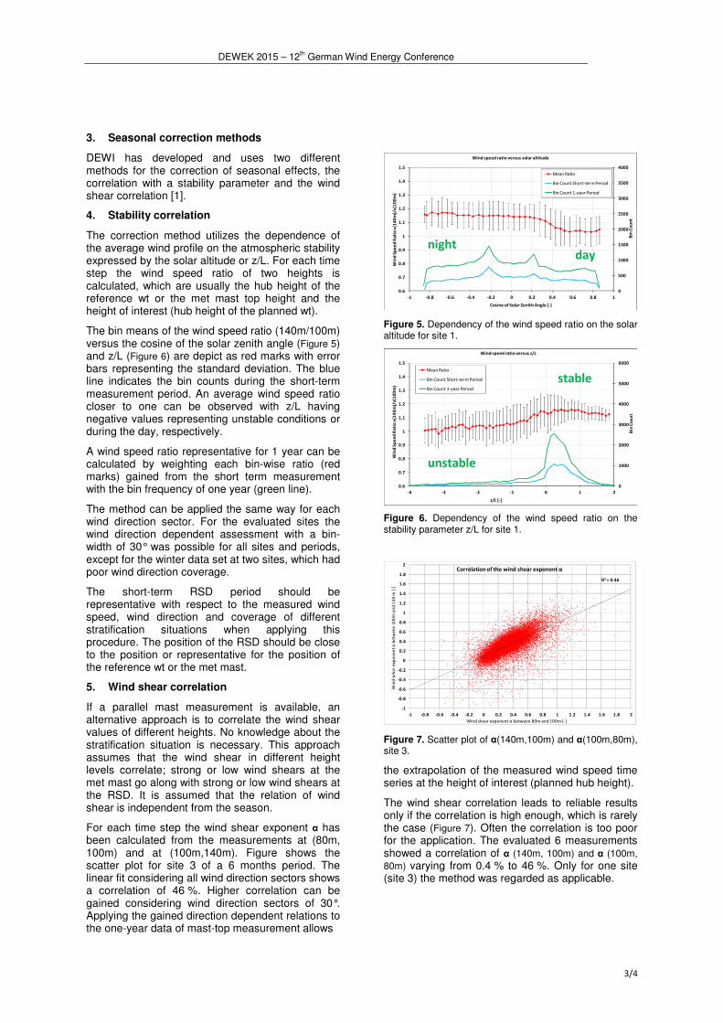
The bin means of the wind speed ratio (140m/100m) versus the cosine of the solar zenith angle (Figure 5) and z/L (Figure 6) are depict as red marks with error bars representing the standard deviation. The blue line indicates the bin counts during the short-term measurement period. An average wind speed ratio closer to one can be observed with z/L having negative values representing unstable conditions or during the day, respectively.

A wind speed ratio representative for 1 year can be calculated by weighting each bin-wise ratio (red marks) gained from the short term measurement with the bin frequency of one year (green line).

The method can be applied the same way for each wind direction sector. For the evaluated sites the wind direction dependent assessment with a bin-width of 30° was possible for all sites and periods, except for the winter data set at two sites, which had poor wind direction coverage.

The short-term RSD period should be representative with respect to the measured wind speed, wind direction and coverage of different stratification situations when applying this procedure. The position of the RSD should be close to the position or representative for the position of the reference wt or the met mast.

5. Wind shear correlation

If a parallel mast measurement is available, an alternative approach is to correlate the wind shear values of different heights. No knowledge about the stratification situation is necessary. This approach assumes that the wind shear in different height levels correlate; strong or low wind shears at the met mast go along with strong or low wind shears at the RSD. It is assumed that the relation of wind shear is independent from the season.

For each time step the wind shear exponent α has been calculated from the measurements at (80m, 100m) and at (100m,140m). Figure shows the scatter plot for site 3 of a 6 months period. The linear fit considering all wind direction sectors shows a correlation of 46 %. Higher correlation can be gained considering wind direction sectors of 30°. Applying the gained direction dependent relations to the one-year data of mast-top measurement allows

Figure 5. Dependency of the wind speed ratio on the solar altitude for site 1.

Figure 6. Dependency of the wind speed ratio on the stability parameter z/L for site 1.

Figure 7. Scatter plot of α(140m,100m) and α(100m,80m), site 3.

the extrapolation of the measured wind speed time series at the height of interest (planned hub height).

The wind shear correlation leads to reliable results only if the correlation is high enough, which is rarely the case (Figure 7). Often the correlation is too poor for the application. The evaluated 6 measurements showed a correlation of α (140m, 100m) and α (100m,

80m) varying from 0.4 % to 46 %. Only for one site (site 3) the method was regarded as applicable.

0

500

1000

1500

2000

2500

3000

3500

4000

0.6

0.7

0.8

0.9

1

1.1

1.2

1.3

1.4

1.5

-1 -0.8 -0.6 -0.4 -0.2 0 0.2 0.4 0.6 0.8 1

Bin

Co

un

t

Win

d S

pe

ed

Ra

tio

v(1

40

m)/

v(1

00

m)

Cosine of Solar Zenith Angle [-]

Wind speed ratio versus solar altitude

Mean Ratio

Bin Count Short-term Period

Bin Count 1-year Period

0

1000

2000

3000

4000

5000

6000

0.6

0.7

0.8

0.9

1

1.1

1.2

1.3

1.4

1.5

-4 -3 -2 -1 0 1 2

Bin

Co

un

t

Win

d S

pe

ed

Ra

tio

v(1

40

m)/

v(1

00

m)

z/L [-]

Wind speed ratio versus z/L

Mean Ratio

Bin Count Short-term Period

Bin Count 1-year Period

R² = 0.46

-1

-0.8

-0.6

-0.4

-0.2

0

0.2

0.4

0.6

0.8

1

1.2

1.4

1.6

1.8

2

-1 -0.8 -0.6 -0.4 -0.2 0 0.2 0.4 0.6 0.8 1 1.2 1.4 1.6 1.8 2

Win

d s

eh

ar

exp

on

en

t α

be

twe

en

10

0m

an

d 1

40

m [

-]

Wind shear exponent α between 80m and 100m [-]

Correlation of the wind shear exponent α

day night

stable

unstable

DEWEK 2015 – 12th German Wind Energy Conference

4/4

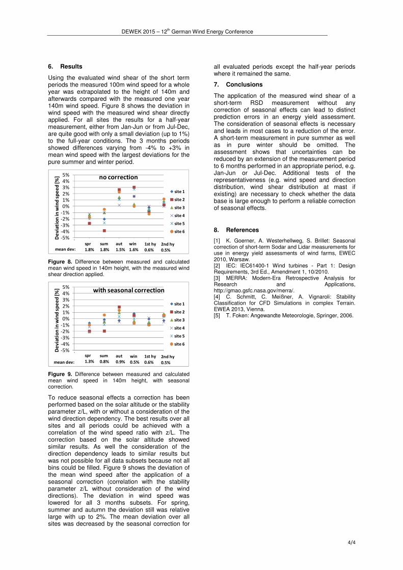
6. Results

Using the evaluated wind shear of the short term periods the measured 100m wind speed for a whole year was extrapolated to the height of 140m and afterwards compared with the measured one year 140m wind speed. Figure 8 shows the deviation in wind speed with the measured wind shear directly applied. For all sites the results for a half-year measurement, either from Jan-Jun or from Jul-Dec, are quite good with only a small deviation (up to 1%) to the full-year conditions. The 3 months periods showed differences varying from -4% to +3% in mean wind speed with the largest deviations for the pure summer and winter period.

Figure 8. Difference between measured and calculated mean wind speed in 140m height, with the measured wind shear direction applied.

Figure 9. Difference between measured and calculated mean wind speed in 140m height, with seasonal correction.

To reduce seasonal effects a correction has been performed based on the solar altitude or the stability parameter z/L, with or without a consideration of the wind direction dependency. The best results over all sites and all periods could be achieved with a correlation of the wind speed ratio with z/L. The correction based on the solar altitude showed similar results. As well the consideration of the direction dependency leads to similar results but was not possible for all data subsets because not all bins could be filled. Figure 9 shows the deviation of the mean wind speed after the application of a seasonal correction (correlation with the stability parameter z/L without consideration of the wind directions). The deviation in wind speed was lowered for all 3 months subsets. For spring, summer and autumn the deviation still was relative large with up to 2%. The mean deviation over all sites was decreased by the seasonal correction for

all evaluated periods except the half-year periods where it remained the same.

7. Conclusions

The application of the measured wind shear of a short-term RSD measurement without any correction of seasonal effects can lead to distinct prediction errors in an energy yield assessment. The consideration of seasonal effects is necessary and leads in most cases to a reduction of the error. A short-term measurement in pure summer as well as in pure winter should be omitted. The assessment shows that uncertainties can be reduced by an extension of the measurement period to 6 months performed in an appropriate period, e.g. Jan-Jun or Jul-Dec. Additional tests of the representativeness (e.g. wind speed and direction distribution, wind shear distribution at mast if existing) are necessary to check whether the data base is large enough to perform a reliable correction of seasonal effects.

8. References

[1] K. Goerner, A. Westerhellweg, S. Brillet: Seasonal correction of short-term Sodar and Lidar measurements for use in energy yield assessments of wind farms, EWEC 2010, Warsaw. [2] IEC: IEC61400-1 Wind turbines - Part 1: Design Requirements, 3rd Ed., Amendment 1, 10/2010. [3] MERRA: Modern-Era Retrospective Analysis for Research and Applications, http://gmao.gsfc.nasa.gov/merra/. [4] C. Schmitt, C. Meißner, A. Vignaroli: Stability Classification for CFD Simulations in complex Terrain. EWEA 2013, Vienna. [5] T. Foken: Angewandte Meteorologie, Springer, 2006.

-5%

-4%

-3%

-2%

-1%

0%

1%

2%

3%

4%

5%

0 1 2 3 4 5 6De

via

tio

n in

win

d s

pe

ed

[%

] no correction

site 1

site 2

site 3

site 4

site 5

site 6

sum

1.8%

aut

1.5%

win

1.6%

1st hy

0.6%

2nd hy

0.5%

spr

1.8%mean dev:

-5%

-4%

-3%

-2%

-1%

0%

1%

2%

3%

4%

5%

0 1 2 3 4 5 6

De

via

tio

n in

win

d s

pe

ed

[%

] with seasonal correction

site 1

site 2

site 3

site 4

site 5

site 6

sum

0.8%

aut

0.9%

win

0.5%

1st hy

0.6%

2nd hy

0.5%

spr

1.3%mean dev: