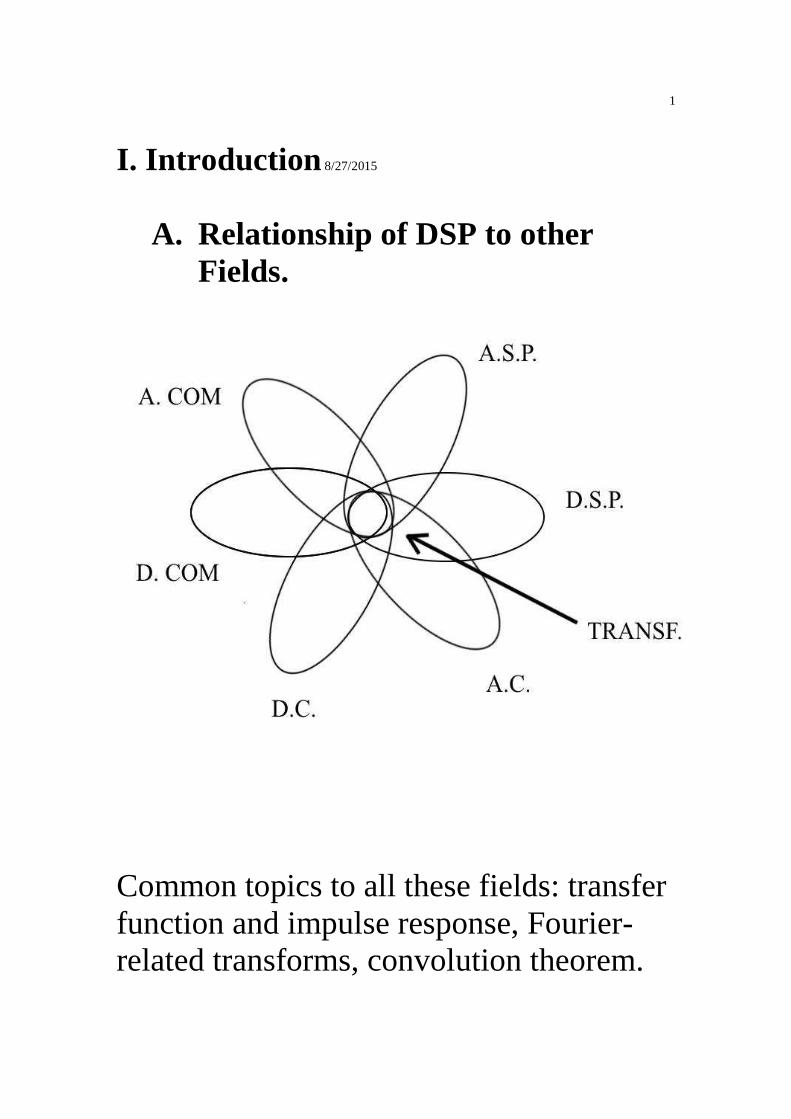
1

I. Introduction 8/27/2015

A. Relationship of DSP to other Fields.

Common topics to all these fields: transfer function and impulse response, Fourier-related transforms, convolution theorem.

2

y(t) = h( )x(t - )d∞

−∞

τ τ τ∫

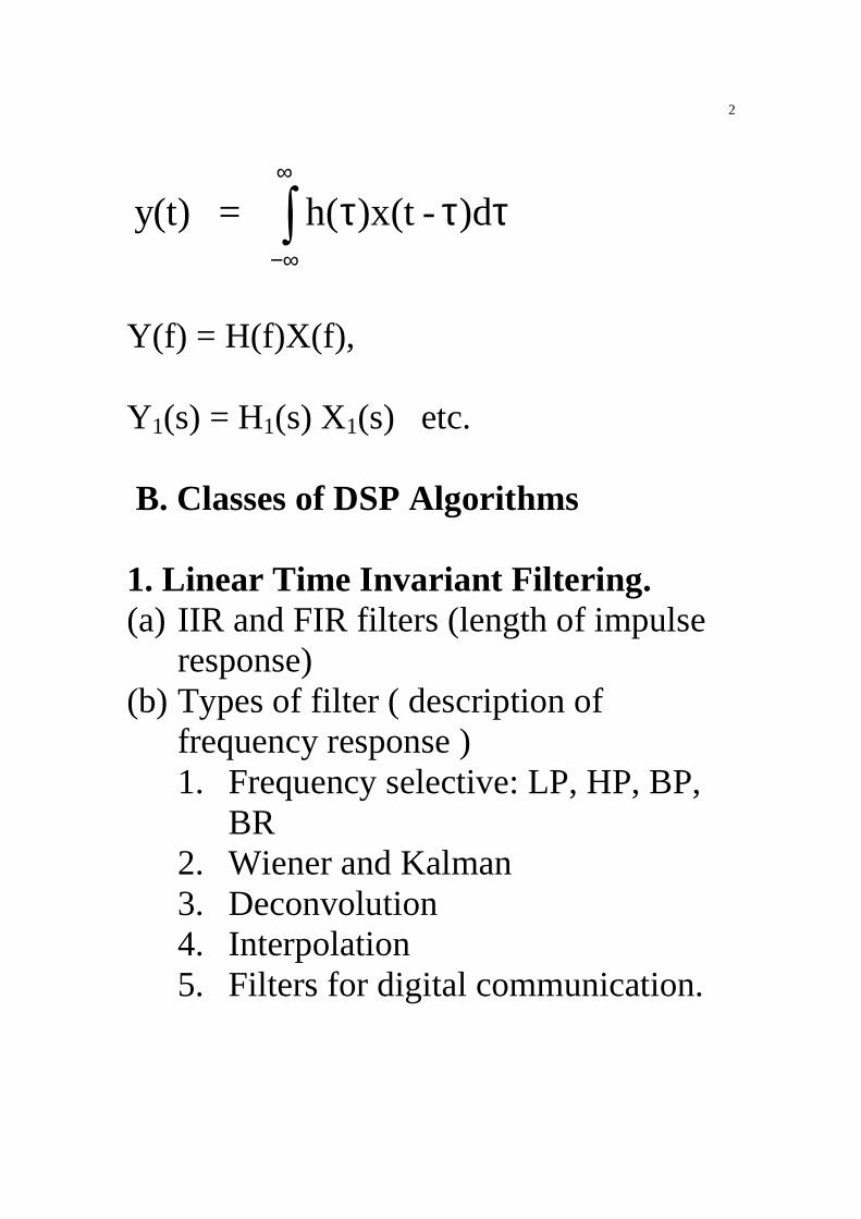
Y(f) = H(f)X(f), Y1(s) = H1(s) X1(s) etc. B. Classes of DSP Algorithms 1. Linear Time Invariant Filtering. (a) IIR and FIR filters (length of impulse

response) (b) Types of filter ( description of

frequency response ) 1. Frequency selective: LP, HP, BP,

BR 2. Wiener and Kalman 3. Deconvolution 4. Interpolation 5. Filters for digital communication.

3

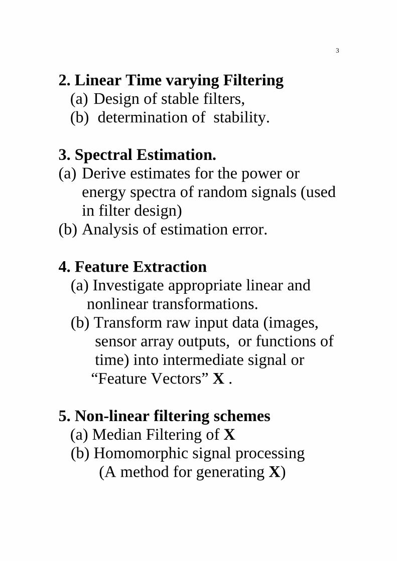
2. Linear Time varying Filtering (a) Design of stable filters, (b) determination of stability.

3. Spectral Estimation. (a) Derive estimates for the power or

energy spectra of random signals (used in filter design)

(b) Analysis of estimation error. 4. Feature Extraction (a) Investigate appropriate linear and nonlinear transformations. (b) Transform raw input data (images, sensor array outputs, or functions of time) into intermediate signal or “Feature Vectors” X . 5. Non-linear filtering schemes (a) Median Filtering of X (b) Homomorphic signal processing (A method for generating X)

4

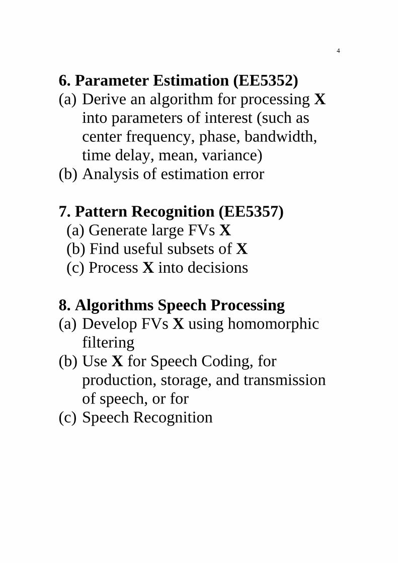
6. Parameter Estimation (EE5352) (a) Derive an algorithm for processing X

into parameters of interest (such as center frequency, phase, bandwidth, time delay, mean, variance)

(b) Analysis of estimation error 7. Pattern Recognition (EE5357) (a) Generate large FVs X (b) Find useful subsets of X (c) Process X into decisions

8. Algorithms Speech Processing (a) Develop FVs X using homomorphic

filtering (b) Use X for Speech Coding, for

production, storage, and transmission of speech, or for

(c) Speech Recognition

5

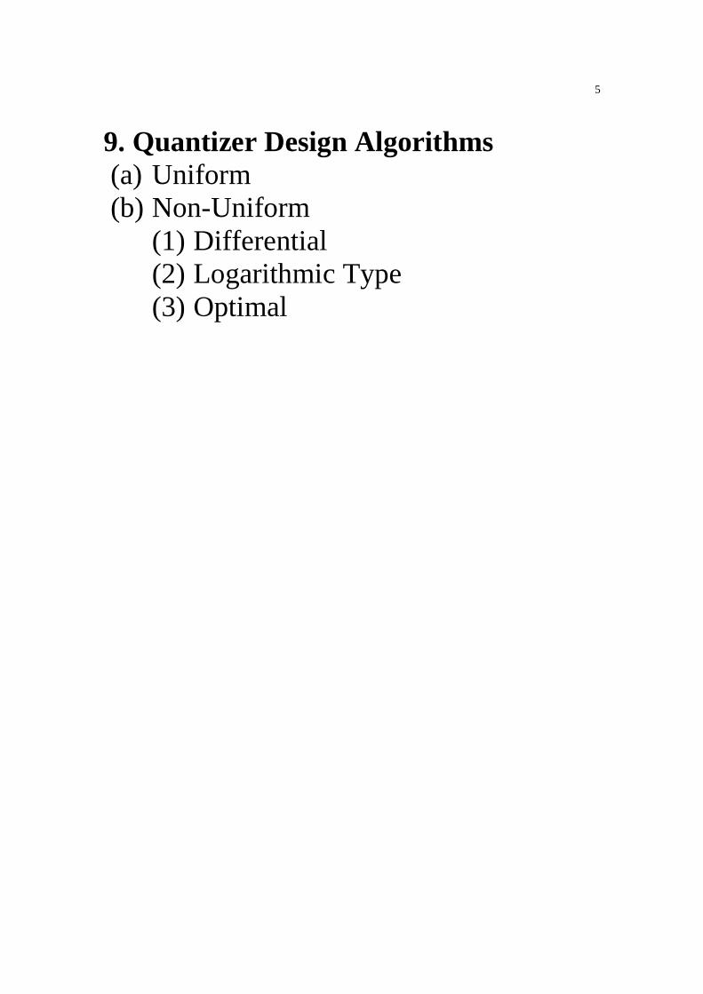
9. Quantizer Design Algorithms (a) Uniform (b) Non-Uniform

(1) Differential (2) Logarithmic Type (3) Optimal

6

B. Types of Hardware

(1) Computers: PC up to super computers (2) Array Processors (perform repetitive

operations very fast, sometimes in parallel)

(3) Switched capacitors filters. (4) FFT chips. DSP chips TMS 32010 TI (5) Filter Chips. (6) Special Purpose Machines.

7

D. DSP Example: NML - Nuclear Magnetic Logging In well-logging, a string of sondes is lowered into a borehole. As the string is pulled up, the sondes take measurements and relay them uphole, where the measurements are plotted on graphs or "logs." Together, graphs of porosity versus depth and conductivity versus depth can be used to: (1) Locate fluid and (2) Distinguish oil from saltwater or fresh water. The NML sonde uses earth's field NMR to detect hydrogen nuclei in fluid (oil or water). The resulting log yields an estimate of porosity versus depth.

8

1. Sketch

9

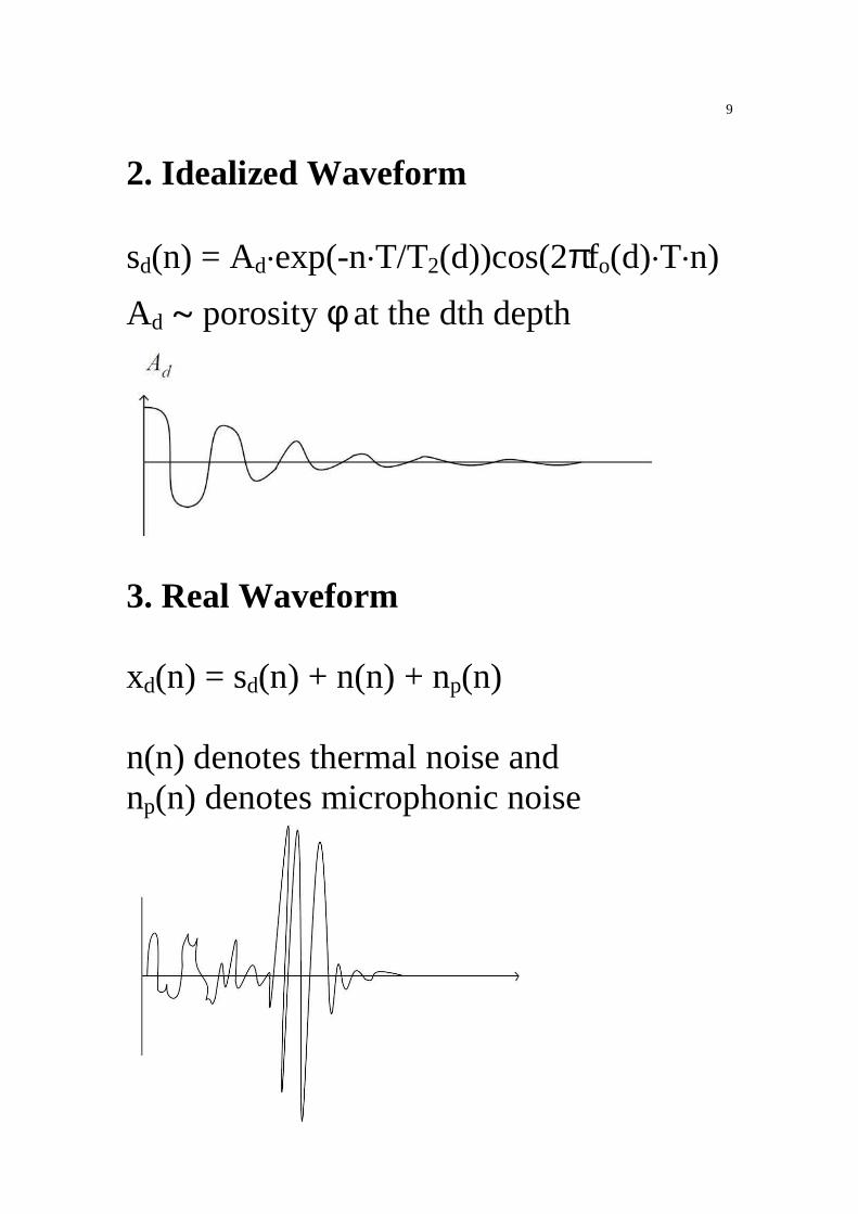
2. Idealized Waveform sd(n) = Ad⋅exp(-n⋅T/T2(d))cos(2πfo(d)⋅T⋅n)

Ad ~ porosity φ at the dth depth

3. Real Waveform xd(n) = sd(n) + n(n) + np(n) n(n) denotes thermal noise and np(n) denotes microphonic noise

10

4. DSP of NML Waveforms Block Diagram

11

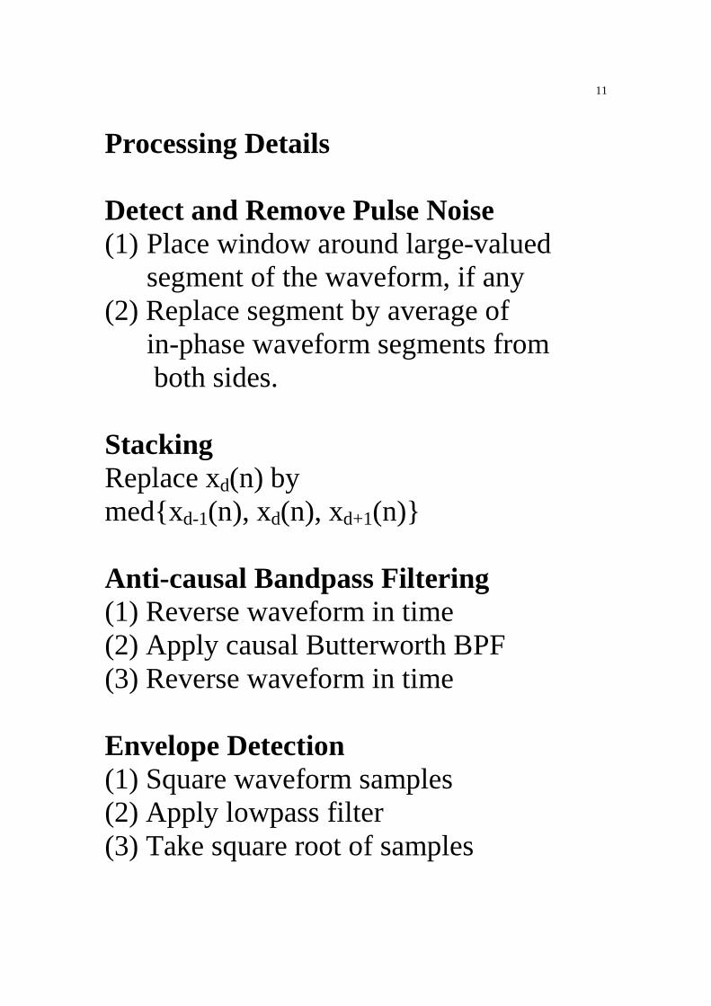
Processing Details Detect and Remove Pulse Noise (1) Place window around large-valued

segment of the waveform, if any (2) Replace segment by average of

in-phase waveform segments from both sides.

Stacking Replace xd(n) by med{xd-1(n), xd(n), xd+1(n)} Anti-causal Bandpass Filtering (1) Reverse waveform in time (2) Apply causal Butterworth BPF (3) Reverse waveform in time Envelope Detection (1) Square waveform samples (2) Apply lowpass filter (3) Take square root of samples

12

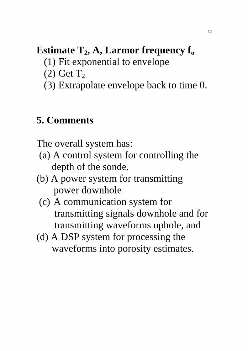
Estimate T2, A, Larmor frequency fo (1) Fit exponential to envelope (2) Get T2 (3) Extrapolate envelope back to time 0.

5. Comments The overall system has: (a) A control system for controlling the depth of the sonde, (b) A power system for transmitting

power downhole (c) A communication system for transmitting signals downhole and for transmitting waveforms uphole, and (d) A DSP system for processing the waveforms into porosity estimates.

13

II. Review of Relevant Math Topics A. Complex Arithmetic j= √-1 1. Rectangular Co-ordinates.

C = a + jb where a, b ∈ R and C ∈ C Re (C) = a, Im(C) = b, not jb. 2. Polar Co-ordinates

C= R ∠θ = R ejθ = R exp(jθ) Using Euler’s Formula, R exp(jθ) = R cos(θ) + j R sin (θ)

14

R, θ ∈ R R ≥ 0, θ in radians. 3. Conversion from Rectangular to Polar a = R cos(θ), b = R sin(θ) R = √a2 + b2 = |C| ( a2 + b2 ) = R2(cos2(θ)+ sin2(θ))= R2 tan (θ) = opposite / adjacent = b/a Sketch

15

θ = tan-1(b/a) = tan-1( Im(C) / Re(C) ) -π/2 ≤ tan-1(x) ≤ π / 2. tan-1(b/a) = tan-1(-b / -a) If Re( C ) is negative, we can add π to θ to correct it. ∴ θ = tan-1(b /a ) + π u (-a) where u(x) is the unit step function. 4. Basic Operations Addition (a + jb) + (c + jd) = ( a+c) + j(b+d) Multiplication (a+jb) (c+jd) = (ac-bd) + j(bc+ad) R1 e

jθ1 • R2 ejθ2 = R1 R2 e

j(θ1 + θ2)

16

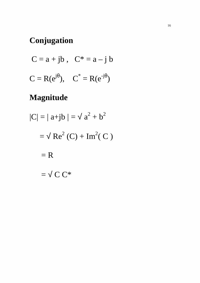
Conjugation C = a + jb , C* = a – j b C = R(ejθ), C* = R(e-jθ) Magnitude |C| = | a+jb | = √ a2 + b2 = √ Re2 (C) + Im2( C ) = R

= √ C C*

17

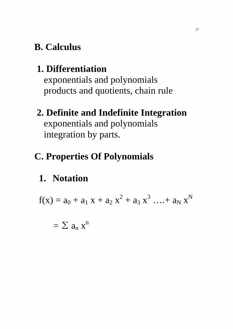
B. Calculus 1. Differentiation exponentials and polynomials products and quotients, chain rule 2. Definite and Indefinite Integration exponentials and polynomials integration by parts. C. Properties Of Polynomials 1. Notation f(x) = a0 + a1 x + a2 x

2 + a3 x3 ….+ aN xN

= ∑ an xn

18

Example f(x) = 1 + 3x + 5x2 + 2 x5 a0 = 1, a1 = 3, a2 = 5, a3 = 0, a4 = 0, a5 = 2 2. Factoring Fundamental Theorem of Algebra:

The zeroes zn can be real or complex. Example x2 – 5x + 6 = (x-2) (x-3)

NNn

n nn=0 n=1

f(x) = a x = K (x - z )⋅∑ ∏

19

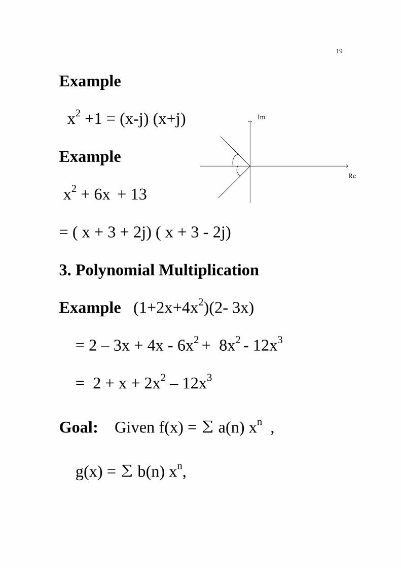
Example x2 +1 = (x-j) (x+j) Example x2 + 6x + 13 = ( x + 3 + 2j) ( x + 3 - 2j) 3. Polynomial Multiplication Example (1+2x+4x2)(2- 3x) = 2 – 3x + 4x - 6x2 + 8x2 - 12x3 = 2 + x + 2x2 – 12x3

Goal: Given f(x) = ∑ a(n) xn ,

g(x) = ∑ b(n) xn,

20

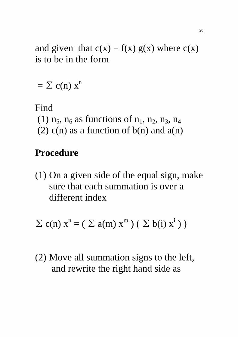
and given that c(x) = f(x) g(x) where c(x) is to be in the form

= ∑ c(n) xn Find (1) n5, n6 as functions of n1, n2, n3, n4 (2) c(n) as a function of b(n) and a(n) Procedure (1) On a given side of the equal sign, make

sure that each summation is over a different index

∑ c(n) xn = ( ∑ a(m) xm ) ( ∑ b(i) xi ) ) (2) Move all summation signs to the left,

and rewrite the right hand side as

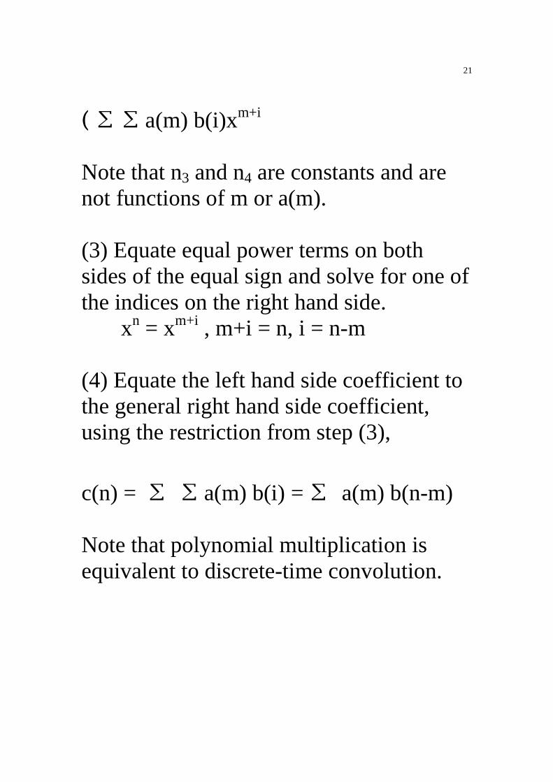
21

( ∑ ∑ a(m) b(i)xm+i Note that n3 and n4 are constants and are not functions of m or a(m). (3) Equate equal power terms on both sides of the equal sign and solve for one of the indices on the right hand side. xn = xm+i , m+i = n, i = n-m (4) Equate the left hand side coefficient to the general right hand side coefficient, using the restriction from step (3),

c(n) = ∑ ∑ a(m) b(i) = ∑ a(m) b(n-m) Note that polynomial multiplication is equivalent to discrete-time convolution.

22

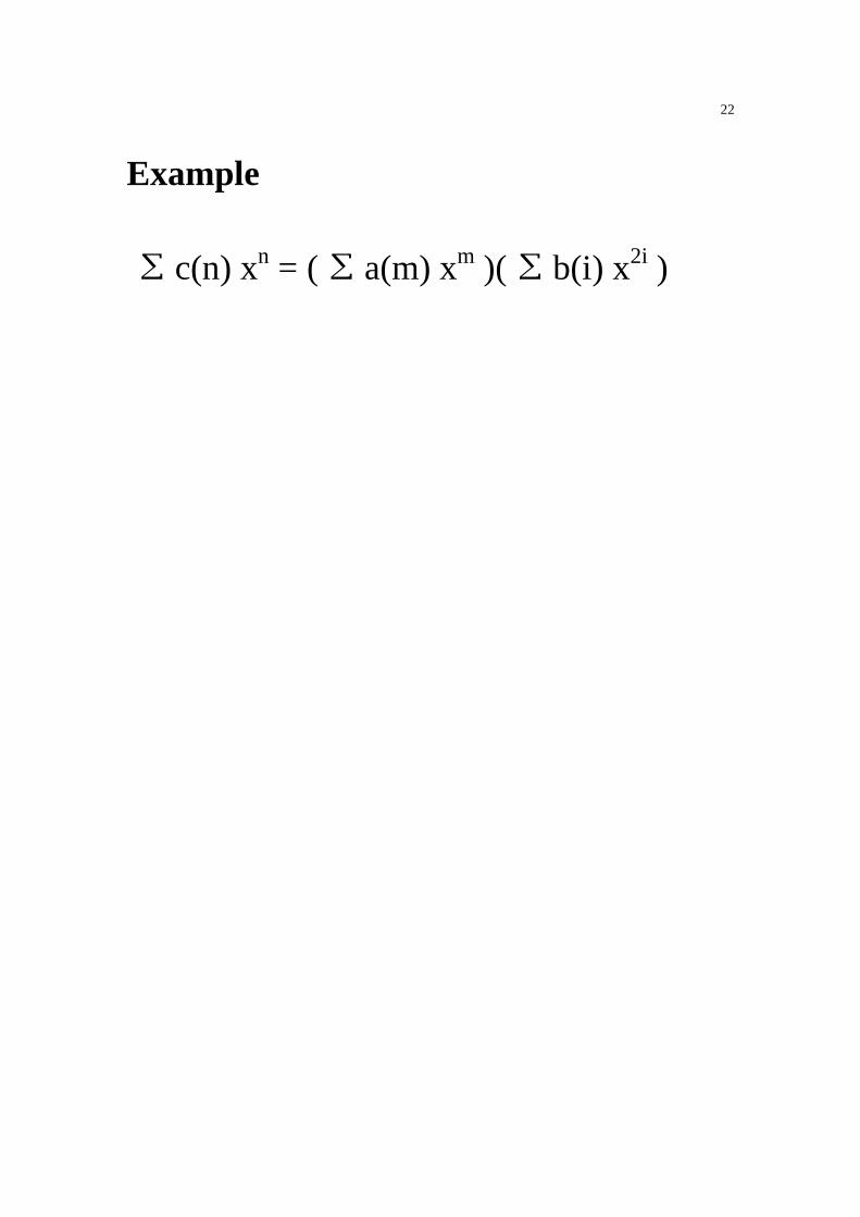
Example

∑ c(n) xn = ( ∑ a(m) xm )( ∑ b(i) x2i )

23

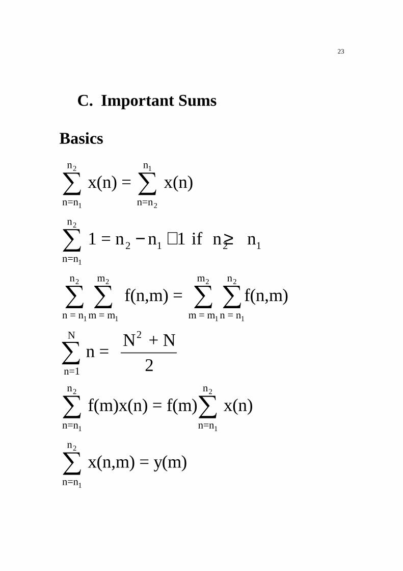
C. Important Sums

Basics

2 1

1 2

2

1

2 2 2 2

1 1 1 1

2 2

1 1

2

1

n n

n=n n=n

n

2 1 2 1n=n

n m m n

n = n m = m m = m n = n

2N

n=1

n n

n=n n=n

n

n=n

x(n) = x(n)

1 = n n 1 if n n

f(n,m) = f(n,m)

N + N n =

2

f(m)x(n) = f(m) x(n)

x(n,m) = y(m)

− + ≥

∑ ∑

∑

∑ ∑ ∑ ∑

∑

∑ ∑

∑

24

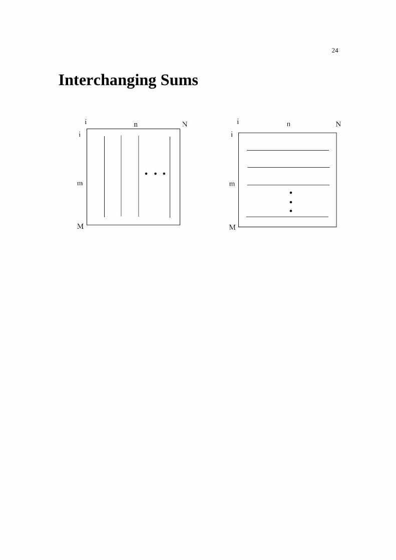
Interchanging Sums

25

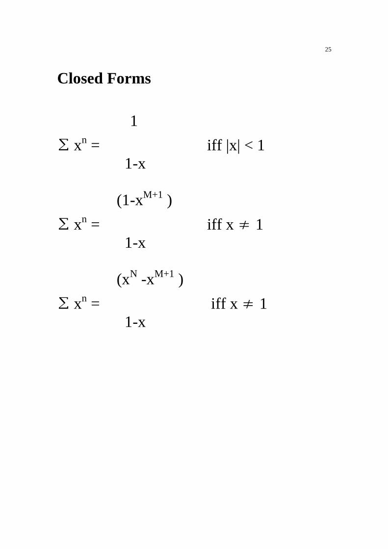
Closed Forms

1

∑ xn = iff |x| < 1 1-x (1-xM+1 )

∑ xn = iff x ≠ 1 1-x (xN -xM+1 )

∑ xn = iff x ≠ 1 1-x

26

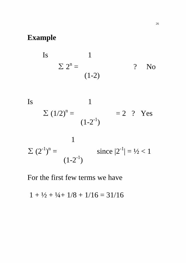
Example Is 1

∑ 2n = ? No (1-2) Is 1

∑ (1/2)n = = 2 ? Yes (1-2-1) 1

∑ (2-1)n = since |2-1| = ½ < 1 (1-2-1) For the first few terms we have 1 + ½ + ¼+ 1/8 + 1/16 = 31/16

27

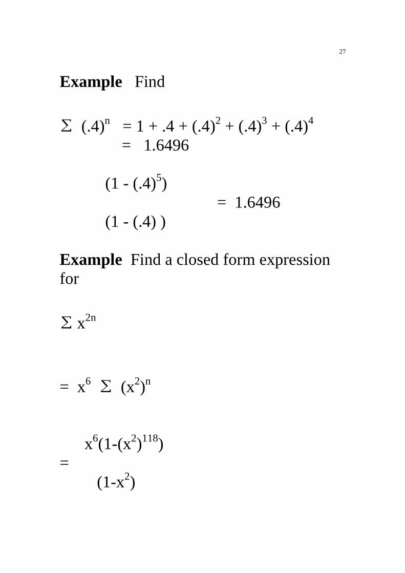
Example Find

∑ (.4)n = 1 + .4 + (.4)2 + (.4)3 + (.4)4 = 1.6496 (1 - (.4)5) = 1.6496 (1 - (.4) ) Example Find a closed form expression for

∑ x2n

= x6 ∑ (x2)n x6(1-(x2)118) = (1-x2)

28

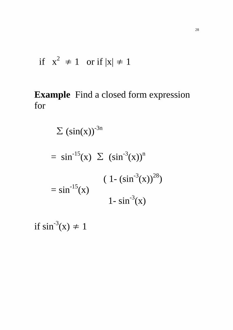
if x2 ≠ 1 or if |x| ≠ 1 Example Find a closed form expression for

∑ (sin(x))-3n

= sin-15(x) ∑ (sin-3(x))n ( 1- (sin-3(x))28) = sin-15(x) 1- sin-3(x)

if sin-3(x) ≠ 1

29

Example ∑ sin (nx) Example

∑ an bm-3n

30

E. Useful Functions

δ(n) = 1 if n =0 0 elsewhere δ(n-3) = 1 if (n-3) = 0 0 elsewhere Sifting Property x(n) = ∑ x(m) δ(n-m) Example Give a function that specifies x(n) as x(n) = n2 x(n) = ∑ m2 δ(n-m)

31

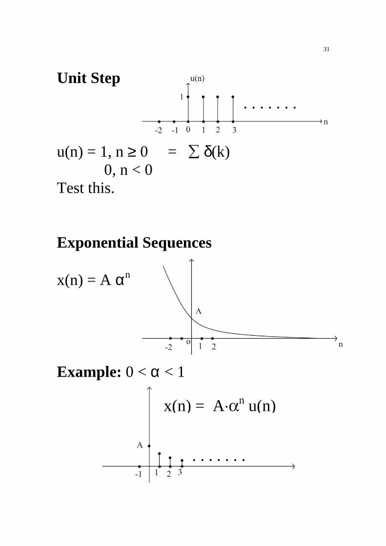
Unit Step u(n) = 1, n ≥ 0 = ∑ δ(k) 0, n < 0 Test this. Exponential Sequences x(n) = A αn Example: 0 < α < 1

. . . . . . .

. . . . . . .

x(n) = A⋅αn u(n)

32

Example Sketch for α < -1

Example Complex exponential sequence. α = Reiθ Complex exponential sequence.

x(n)

n

x(n) = (-2)n u(n)

33

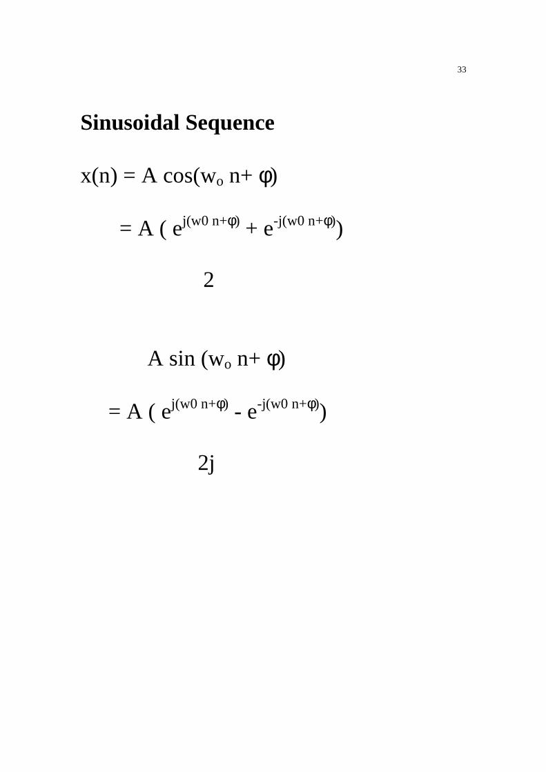
Sinusoidal Sequence x(n) = A cos(wo n+ φ) = A ( ej(w0 n+φ) + e-j(w0 n+φ)) 2 A sin (wo n+ φ) = A ( ej(w0 n+φ) - e-j(w0 n+φ)) 2j

34

Periodic Sequences x(n) = x(n+N) for all n. N = period N must be an integer.

Example Let x(n) = A cos (wo

n + φ). Under what condition is x(n) periodic ? A cos (wo

n + φ) = A cos (wo (n+N) + φ) woN = 2πk (1) wo = 2πk/N , given N. (2) N = 2πk/wo . Periodic if N is an integer

35

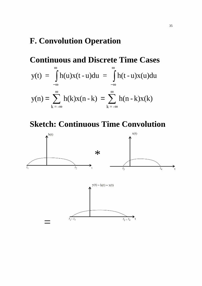
F. Convolution Operation Continuous and Discrete Time Cases

k = - k = -

y(t) = h(u)x(t - u)du = h(t - u)x(u)du

y(n) h(k)x(n - k) h(n - k)x(k)

∞ ∞

−∞ −∞∞ ∞

∞ ∞

= =

∫ ∫

∑ ∑

Sketch: Continuous Time Convolution

*

=

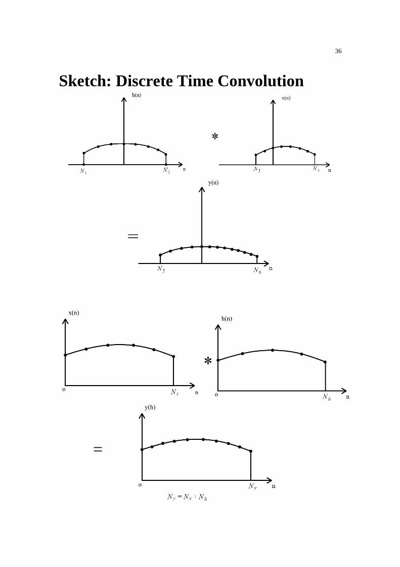
36

=

Sketch: Discrete Time Convolution

37

Pseudocode for Discrete Time Convolution of Causal Signals (1) Standard Offline Convolution y(n) = ∑ h(k) x(n-k) = ∑ h(n-k) x(k) Ny = Nh + Nx For 0 ≤ n ≤ Ny y(n) = 0 For 0 ≤ k ≤ Nh

m = n-k If(m ≥ 0 and m ≤ Nx)Then y(n) = y(n) + h(k)⋅x(n-k) Endif End End

38

(2) Alternate Offline Convolution Ny = Nh + Nx

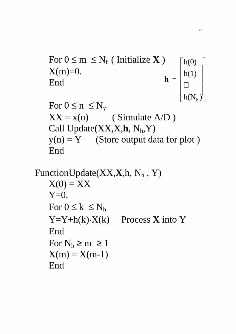
For 0 ≤ n ≤ Ny y(n) = 0 End For 0 ≤ n ≤ Nx For 0 ≤ m ≤ Nh y(n+m) = y(n+m) + h(m)⋅x(n) End End (3) Real-Time Version for Finite Length h(n) Idea: Store several delayed samples of x(n) in a vector X, which can be called an: (a) Intermediate signal vector (b) State vector (c) Feature Vector

39

For 0 ≤ m ≤ Nh ( Initialize X ) X(m)=0. End For 0 ≤ n ≤ Ny XX = x(n) ( Simulate A/D ) Call Update(XX,X,h, Nh,Y) y(n) = Y (Store output data for plot ) End FunctionUpdate(XX,X,h, Nh , Y) X(0) = XX Y=0. For 0 ≤ k ≤ Nh Y=Y+h(k)⋅X(k) Process X into Y End For Nh ≥ m ≥ 1 X(m) = X(m-1) End

h

h(0)

h(1) =

h(N )

⋅

h