Rapid function approximation by modiﬁed Fourier seriesdaan/research/MFS.pdf · Rapid function...

1

Rapid function approximation bymodified Fourier series

Daan Huybrechs and Sheehan Olver

Abstract

We review a set of algorithms and techniques to approximate smooth

functions on a domain Ω ⊂ Rd by an expansion in eigenfunctions of

the Laplacian. We refer to such expansions as modified Fourier series.

These series converge pointwise everywhere in the domain of approxima-

tion, including on the boundary, at an algebraic rate that is essentially

arbitrary. The computational complexity of the transformation is only

linear in the number of terms of the expansion. Moreover, additional

terms can be computed adaptively and efficiently.

1.1 Introduction

The subject of this review paper is the approximation of smooth func-

tions. The method of approximation is quite simple: a smooth function

f on a domain Ω is expanded into eigenfunctions un of the Laplace

operator, subject to Neumann boundary conditions:

−∆un(x) = λnun(x), x ∈ Ω,∂un

∂ν(x) = 0, x ∈ ∂Ω.

(1.1)

On the face of it, this may not appear to be a recent research topic.

It has long been known that such eigenfunctions are orthogonal and

dense in L2[Ω], making them ideally suitable for series expansions of

quite arbitrary functions on domains with great generality. The Laplace

operator has probably received the widest study among all partial differ-

ential operators. Yet, for the purpose of numerical approximation, it is

usually neglected in favour of alternative approaches. Two well-known

1

2 D. Huybrechs and S. Olver

and successful examples for univariate functions are the approximation

by Chebyshev polynomials, for smooth functions on an interval, and the

FFT algorithm, for smooth functions that are in addition periodic. The

recent research in modified Fourier series brings two properties that are

indispensable for any approximation method: fast algorithms and rapid

convergence, thereby adding competitiveness to generality.

One of the main results is an O(m) algorithm for the computation of

the first m coefficients in the series. This result holds for periodic and

non-periodic functions alike. Needless to say, this computational com-

plexity compares favourably to the alternatives mentioned above. The

result has been made possible primarily through the advent of efficient

computational schemes for highly oscillatory integrals. Such schemes

are the subject of a separate review paper in this same volume, to which

the interested reader is referred [9]. The connection to modified Fourier

series becomes obvious once we observe that Laplace–Neumann eigen-

functions become increasingly oscillatory. Hence, the coefficients of the

series are given by increasingly oscillatory integrals. The most important

development in the evaluation of highly oscillatory integrals is, arguably,

the Filon-type method [10]. We will show how Filon-type methods can

be extended and adapted to the setting of modified Fourier series. The

O(m) algorithm then follows immediately.

The second property is rapid convergence. In unaltered form, the al-

gorithm briefly described above yields O(m−2) convergence, pointwise

in the interior of Ω, and O(m−1) convergence on the boundary ∂Ω.

Note that the FFT-algorithm on an interval [a, b], though ideally suited

for periodic functions, yields only O(m−1) pointwise convergence for

non-periodic functions in the interior, and no convergence at all at the

boundary points. The convergence of modified Fourier series can be im-

proved in several ways. In this paper we discuss two approaches: faster

initial convergence through the use of eigenfunctions of polyharmonic

operators and accelerated convergence through the use of polynomial

subtraction. A possible third approach is based on extrapolation [14].

The main results in the approximation by modified Fourier series have

been established in a series of papers [11, 12, 13, 14, 8]. The current

paper mostly follows the same pattern of developments. We start by

reviewing one-dimensional approximation in §1.2. The generalization in

the direction of polyharmonic operators is discussed in §1.3. A gener-

alization in a different direction, to multivariate approximation, is re-

Rapid function approximation by modified Fourier series 3

viewed in §1.4. Finally, we treat the acceleration of convergence in §1.5.

We end with some concluding remarks in §1.6.

1.2 Univariate approximation

The simplest setting is that of a function f defined on the interval Ω :=

[−1, 1]. This univariate setting is well suited to motivate the use of

Laplace–Neumann expansions and to appreciate their basic properties.

1.2.1 Laplace–Neumann expansions

The standard Fourier series of f on the interval [−1, 1] is given by

1

2fC0 +

∞∑

n=1

fCn cosπnx + fD

n sinπnx,

where

fCn =

∫ 1

−1

f(x) cosπnxdx, fDn =

∫ 1

−1

f(x) sin πnxdx.

Let us assume that the function f is non-periodic. In that case, the

Fourier coefficients as defined above behave like fCn = O(n−2) and fD

n =

O(n−1) for n ≫ 1. We note that the sine coefficients are primarily

responsible for the slow convergence rate of the Fourier series.

The expansion in eigenfunctions of the Laplace operator, as defined

by (1.1), leads to a very similar series:

1

2fC0 +

∞∑

n=1

fCn cosπnx + fS

n sin π(n − 12 )x, (1.2)

where

fSn =

∫ 1

−1

f(x) sin π(n − 12 )xdx. (1.3)

The only difference compared to classical Fourier is a shift by 12 in the

argument of the sine functions, hence the name modified Fourier series.

This small change suffices to yield O(n−2) behaviour of the correspond-

ing coefficients in the series when f is differentiable and its derivative

has bounded variation. Moreover, both fC0 and fS

0 have an even expan-

sion if f is sufficiently smooth. This follows from integration by parts

and establishes a pattern for the upcoming generalizations.


100

101

102

10−15

10−10

10−5

100

(a) Absolute size of the coefficients

fCn (full lines) and fS

n (dashed lines)

−1 −0.5 0 0.5 110

−15

10−10

10−5

100

(b) Approximation error for m = 30terms on the interval (−1, 1)

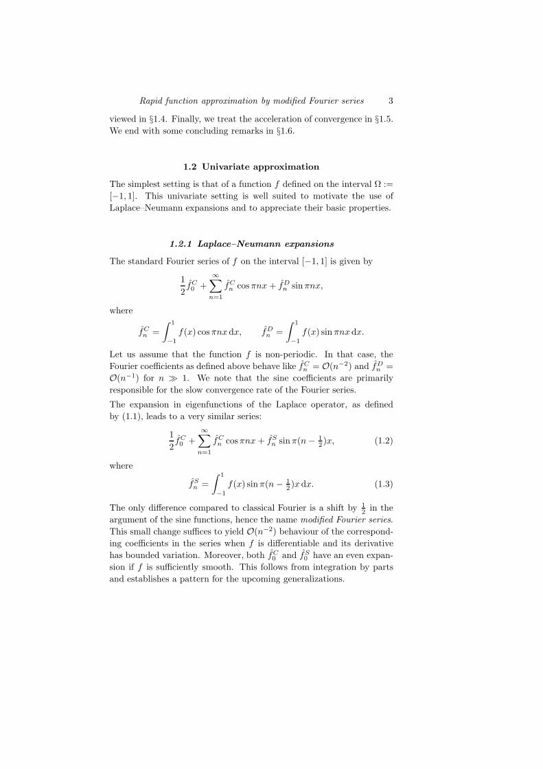
Fig. 1.1. Approximation of f(x) = cos(x + 1) sin(x + 1) by a modified Fourierseries. Polynomial subtraction was used with 0, 1 and 2 steps (from top tobottom), leading to convergence rates of O(m−2), O(m−4) and O(m−6).

Theorem 1.1 If f ∈ C∞[−1, 1] then for n ≫ 1 we have

fCn ∼ (−1)n

∑

∞

k=0(−1)k

(nπ)2k+2 [f (2k+1)(1) − f (2k+1)(−1)],

fSn ∼ (−1)n−1

∑

∞

k=0(−1)k

[(n− 12)π]2k+2 [f (2k+1)(1) + f (2k+1)(−1)].

Proof Integrating expression (1.3) by parts once yields

fSn = − f(x) cosπ(n − 1

2 )x

(n − 12 )π

∣

∣

∣

∣

1

−1

+1

(n − 12 )π

∫ 1

−1

f ′(x) cos π(n − 1

2)xdx.

The first term vanishes due to the homogeneous Neumann boundary

conditions. Integrating by parts once more leads to

fSn =

f ′(x) sin π(n − 12 )x

(n − 12 )2π2

∣

∣

∣

∣

1

−1

− 1

(n − 12 )2π2

∫ 1

−1

f (2)(x) sin π(n− 1

2)xdx.

Repeated invocation of integration by parts on the remainder integral

yields the result. The proof for the coefficients fCn is analogous.

It is thus established that the coefficients of the modified Fourier series

(1.2) decay faster than those of a classic Fourier series. We emphasize

the fact that this property essentially follows from the homogeneous

Neumann boundary conditions satisfied by the basis functions.

The asymptotic expansions in Theorem 1.1 also indicate that the coeffi-

cients asymptotically depend only on odd derivatives of f , evaluated at

the two boundary points of the interval [−1, 1]. This observation will be

used later on for efficiently accelerating the decay even further.


The size of the coefficients and the approximation error are illustrated

in Figure 1.1 (top curve). The figure also shows improved decay rates

through polynomial subtraction. This will be discussed later in §1.5.1.

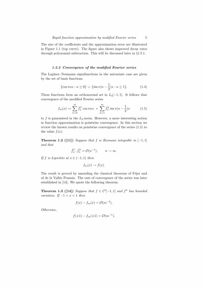
1.2.2 Convergence of the modified Fourier series

The Laplace–Neumann eigenfunctions in the univariate case are given

by the set of basis functions

cosπnx : n ≥ 0 ∪ sinπ(n − 1

2)x : n ≥ 1. (1.4)

These functions form an orthonormal set in L2[−1, 1]. It follows that

convergence of the modified Fourier series

fm(x) :=

m∑

n=0

fCn cosπnx +

m∑

n=1

fSn sin π(n − 1

2)x (1.5)

to f is guaranteed in the L2-norm. However, a more interesting notion

in function approximation is pointwise convergence. In this section we

review the known results on pointwise convergence of the series (1.5) to

the value f(x).

Theorem 1.2 ([11]) Suppose that f is Riemann integrable in [−1, 1]

and that

fCn , fS

n = O(n−1), n → ∞.

If f is Lipschitz at x ∈ (−1, 1) then

fm(x) → f(x).

The result is proved by amending the classical theorems of Fejer and

of de la Vallee Poussin. The rate of convergence of the series was later

established in [14]. We quote the following theorem.

Theorem 1.3 ([14]) Suppose that f ∈ C2[−1, 1] and f ′′ has bounded

variation. If −1 < x < 1 then

f(x) − fm(x) = O(m−2).

Otherwise,

f(±1) − fm(±1) = O(m−1).


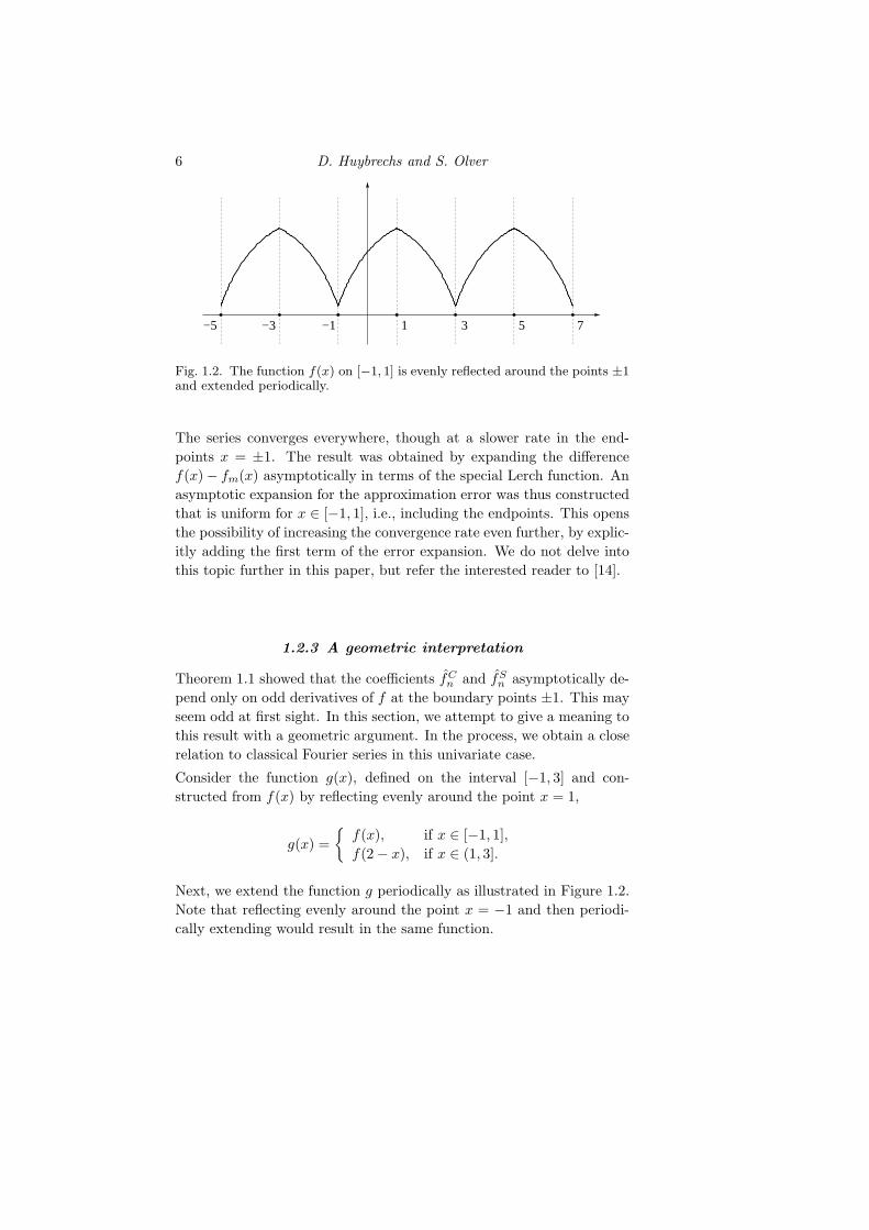
−1 1 3 5 7−3−5

Fig. 1.2. The function f(x) on [−1, 1] is evenly reflected around the points ±1and extended periodically.

The series converges everywhere, though at a slower rate in the end-

points x = ±1. The result was obtained by expanding the difference

f(x) − fm(x) asymptotically in terms of the special Lerch function. An

asymptotic expansion for the approximation error was thus constructed

that is uniform for x ∈ [−1, 1], i.e., including the endpoints. This opens

the possibility of increasing the convergence rate even further, by explic-

itly adding the first term of the error expansion. We do not delve into

this topic further in this paper, but refer the interested reader to [14].

1.2.3 A geometric interpretation

Theorem 1.1 showed that the coefficients fCn and fS

n asymptotically de-

pend only on odd derivatives of f at the boundary points ±1. This may

seem odd at first sight. In this section, we attempt to give a meaning to

this result with a geometric argument. In the process, we obtain a close

relation to classical Fourier series in this univariate case.

Consider the function g(x), defined on the interval [−1, 3] and con-

structed from f(x) by reflecting evenly around the point x = 1,

g(x) =

f(x), if x ∈ [−1, 1],

f(2 − x), if x ∈ (1, 3].

Next, we extend the function g periodically as illustrated in Figure 1.2.

Note that reflecting evenly around the point x = −1 and then periodi-

cally extending would result in the same function.


Now consider the classical Fourier series of g on the interval [−1, 3],

gm(x) =

m∑

n=0

gCn cos

(

2π

4n(x + 1)

)

+

m∑

n=1

gSn sin

(

2π

4n(x + 1)

)

,

where

gCn :=

∫ 3

−1g(x) cos

(

2π4 n(x + 1)

)

dx, n = 0, 1, . . . ,

gSn :=

∫ 3

−1g(x) sin

(

2π4 n(x + 1)

)

dx, n = 1, 2, . . . .

Since g(x) is even on [−1, 3] around the center point x = 1, we have

gSn = 0. One can also easily verify that

fCn = (−1)n gC

2n

2, fS

n = (−1)n gC2n−1

2.

In other words, the modified Fourier series of f is equivalent to the

classical Fourier series of g. Figure 1.2 now explains the importance of

odd derivatives at ±1. If f ′(1) = f ′(−1) = 0, then one sees that the

differentiability of g across the reflection points is increased. Thus, its

Fourier series converges faster. The values of the even derivatives of f

at ±1 are irrelevant, as they do not limit the continuity of g.

We observe that the modified Fourier series of f converges faster if f

can be extended as a smooth and even function across the boundary of

the domain Ω. We will see that this observation generalizes to different

domains Ω. The analogy to Fourier series, unfortunately, does not.

Due to this analogy with Fourier series, one may be tempted to com-

pute the coefficients fCn and fS

n using FFT. The alternative approaches

discussed in the next section are far more accurate however, because the

function g in general will not be a smooth function.

1.2.4 Computation of the coefficients

The coefficients fCn and fS

n are given by integrals that become increas-

ingly oscillatory as n ≫ 1. An account of recent research in efficient

methods for the evaluation of oscillatory integrals is given in [9]. From

the results in that review, it becomes apparent that the coefficients can

be computed at a cost that is asymptotically independent of n. That is,

each coefficient fCn and fS

n can be computed with O(1) evaluations of

f as n ≫ 1. An immediate result is that the first m coefficients can be

computed in O(m) operations.

An additional desire in the setting of modified Fourier series is to reuse


function evaluations of f for the computation of coefficients with varying

values of n. With this goal in mind, we will revisit Filon-type quadrature,

though noting that Levin-type methods are equally applicable [14].

The purpose of so-called exotic quadrature is again to maximize reuse of

function evaluations, this time for the computation of coefficients with

smaller n, in a further attempt to bridge the gap between oscillatory

and non-oscillatory quadrature.

1.2.4.1 Filon-type quadrature

The simplest approximation method for fCn and fS

n is, arguably, a trun-

cation of the asymptotic expansions in Theorem 1.1. For example, we

may define

ACs,n[f ] ∼ (−1)n

s−1∑

k=0

(−1)k

(nπ)2k+2[f (2k+1)(1) − f (2k+1)(−1)],

which corresponds to truncating the expansion for fCn after s terms.

This approximation carries an error of asymptotic order

fCn − AC

s,n[f ] ∼ O(n−2s−2), n ≫ 1. (1.6)

The error has the same size, asymptotically, as the first discarded term

in the expansion. It decreases rapidly as n becomes large.

This asymptotic approximation is not very useful however for small val-

ues of n. The idea of Filon-type quadrature is to maintain high asymp-

totic order, in the sense of (1.6), while also maintaining the classical

notion of polynomial exactness. That is, Filon-type quadrature rules

are exact when f is a polynomial of a certain degree. For general os-

cillatory integrals, this leads to quadrature rules involving derivatives.

Let

−1 = c1 < c2 < . . . < cν = 1

be a set of ν quadrature points with associated multiplicities mk ∈ N.

We construct a polynomial p of degree∑ν

k=1 mk − 1 such that

p(i)(ck) = f (i)(ck), i = 0, 1, . . . , mk − 1, k = 1, 2, . . . , ν.

Then a Filon-type method may be defined by

fCn ≈ QC

n [f ] := pCn =

∫ 1

−1

p(x) cosπnxdx.

This can be expressed in closed form since the moments are known,


which are computable either via integration by parts or the formula (for

k > 0):

∫ 1

−1xk cosπnxdx =

ℜ

(−inπ)−k−1[Γ(1 + k, inπ) − Γ(1 + k,−inπ)]

,

where Γ is the incomplete Gamma function.

In the context of modified Fourier series, this general setting changes

in the following way. The key to obtain high asymptotic order is to

interpolate the odd derivatives of f at the endpoints. In other words, it

is sufficient to interpolate precisely the data on which the early terms in

the asymptotic expansion depend. This leads to a set of interpolation

conditions of the form

p(2i+1)(ck) = f (2i+1)(ck), i = 0, 1, . . . , mk − 1, k = 1, 2, . . . , ν.

Augmented by the condition p(0) = f(0), this interpolation problem has

a unique solution. The corresponding quadrature rules take the form

QCn [f ] :=

ν∑

k=1

mk−1∑

j=0

θCk,j(n)f (2j+1)(ck). (1.7)

This rule has asymptotic error O(n−2s−2) if m1, mν ≥ s. Similar rules

can of course be constructed for the sine coefficients fSn .

The weights θCk,j(n) typically depend on n in an explicit manner. Sub-

stantial insights in the design of Filon-type quadrature methods are de-

veloped in [11, 12, 13], and we refer the reader to those papers for explicit

examples of suitable quadrature rules.

1.2.4.2 Exotic quadrature

For small values of n, the integrals fCn and fS

n to compute are non-

oscillatory in nature. One can resort to any of the known quadrature

schemes for smooth and non-oscillatory functions, such as composite

Gaussian quadrature [6]. Note that for achieving an O(m) algorithm

for the computation of the first m coefficients, it is actually irrelevant

how the first (finitely many) elements are computed. Nevertheless, one

naturally seeks for optimal methods that reduce computation time.

Given that the computation of coefficients for large n requires deriva-

tives at the endpoints, one can reuse this information in the computa-

tion of coefficients for small n. This leads to quadrature rules involving


derivatives that, for lack of an established name, were dubbed exotic

quadrature in [12]. They have the general form

∫ 1

−1

g(x) dx ≈ P [f ] :=

ν∑

k=1

∑

j∈Nmk

δk,jg(j)(ck),

and they are typically applied to the function g(x) = f(x)un(x), where

un(x) is one of the Laplace-Neumann eigenfunctions. We have intro-

duced the sets Nm to illustrate that the information about derivatives

in exotic quadrature may be lacunary. For example, in the case of uni-

variate modified Fourier series, we may define

Nm := 2j + 1m−1j=0 .

The main message embodied in the theory of Filon-type quadrature

and exotic quadrature is that the onset of asymptotic behaviour for

increasing n is quite rapid. It appears that asymptotic accuracy kicks

in for very moderate values of n. It is only reasonable to exploit this.

1.3 Polyharmonic approximation

The importance of imposing homogeneous Neumann boundary condi-

tions in the general setting (1.1) became visible in Theorem 1.1. The

boundary conditions rendered the first term in the asymptotic expan-

sion of the coefficients zero, thus generating faster decay. This obser-

vation leads in a natural way to the first generalization of the theory,

where faster convergence is achieved by imposing higher-order Neumann

boundary conditions. In particular, in this section we are interested in

eigenfunctions of the polyharmonic operator

u(2q) + (−1)q+1α2qu = 0, −1 ≤ x ≤ 1, (1.8)

subject to the Neumann boundary conditions

u(i)(−1) = u(i)(1) = 0, i = q, q + 1, . . . , 2q − 1. (1.9)

Here q is a fixed parameter determining the order of the polyharmonic

operator.

Denote the nth eigenvalue as

κn = (−1)qα2q,


with the corresponding nth eigenfunction denoted as un. Like the mod-

ified Fourier series, the basis of eigenfunctions u1, u2, . . . form an or-

thogonal series with respect to the L2 inner product. Furthermore, they

are dense in L2[−1, 1] [12]. Thus we can successfully utilize them for

function approximation, giving us the expansion

f(x) ∼∞∑

n=1

fnun, for fn =

∫ 1

−1

f(x)un(x) dx.

By repeatedly utilizing integration by parts and assuming that f is (q +

1)-times differentiable, we immediately find that

fn =

∫ 1

−1

f(x)un(x) dx =(−1)q

α2qn

∫ 1

−1

f(x)u(2q)n (x) dx

=1

α2qn

∫ 1

−1

f (q)(x)u(q)n (x) dx

=1

α2qn

[f (q)(1)u(q−1)n (1) − f (q)(−1)u(q−1)

n (−1)]

− 1

α2qn

∫ 1

−1

f (q+1)(x)u(q−1)n (x) dx.

From [12], we know that u(i)n (x) = O(αi

n). Furthermore, we also know

that αn ∼ O(n) [15]. It follows immediately that

fn = O(n−q−1).

Thus we can obtain any algebraic convergence rate by choosing q large

enough.

1.3.1 The basis of eigenfunctions

In this section we will demonstrate how αn and the eigenfunctions un

can be found. For simplicity we focus on the case where q = 2, referring

the interested reader to [12] for the derivation for other values of q.

The first two eigenfunctions are trivial (which we will not include in the

enumeration u1, u2, . . .): 1 and x. It follows immediately from (1.8)

that the other eigenfunctions can be expressed as a sum of exponentials.

In particular, for q = 2 we obtain

u(x) = c1 cosαx + c2 sin αx + c3 coshαx + c4 sinhαx.

Our goal, then, is to find which values of ck and α satisfy the boundary


-1.0 -0.5 0.5 1.0

-1.0

-0.5

0.5

1.0

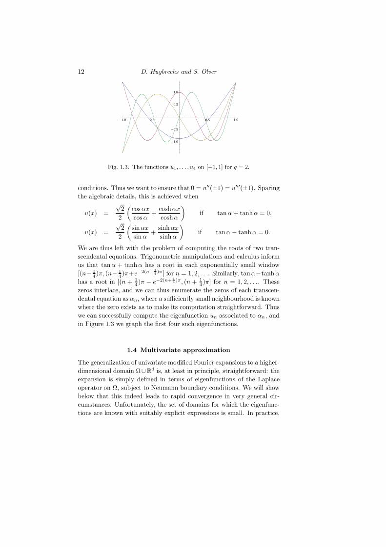
Fig. 1.3. The functions u1, . . . , u4 on [−1, 1] for q = 2.

conditions. Thus we want to ensure that 0 = u′′(±1) = u′′′(±1). Sparing

the algebraic details, this is achieved when

u(x) =

√2

2

(

cosαx

cosα+

coshαx

coshα

)

if tanα + tanhα = 0,

u(x) =

√2

2

(

sinαx

sin α+

sinhαx

sinhα

)

if tanα − tanhα = 0.

We are thus left with the problem of computing the roots of two tran-

scendental equations. Trigonometric manipulations and calculus inform

us that tanα + tanhα has a root in each exponentially small window

[(n− 14 )π, (n− 1

4 )π+e−2(n− 14)π] for n = 1, 2, . . .. Similarly, tanα−tanhα

has a root in [(n + 14 )π − e−2(n+ 1

4)π, (n + 1

4 )π] for n = 1, 2, . . .. These

zeros interlace, and we can thus enumerate the zeros of each transcen-

dental equation as αn, where a sufficiently small neighbourhood is known

where the zero exists as to make its computation straightforward. Thus

we can successfully compute the eigenfunction un associated to αn, and

in Figure 1.3 we graph the first four such eigenfunctions.

1.4 Multivariate approximation

The generalization of univariate modified Fourier expansions to a higher-

dimensional domain Ω∪Rd is, at least in principle, straightforward: the

expansion is simply defined in terms of eigenfunctions of the Laplace

operator on Ω, subject to Neumann boundary conditions. We will show

below that this indeed leads to rapid convergence in very general cir-

cumstances. Unfortunately, the set of domains for which the eigenfunc-

tions are known with suitably explicit expressions is small. In practice,


multivariate modified Fourier expansions are therefore limited to a few

domains. In two dimensions, the list includes ellipses, rectangles, annuli

and a number of different triangles.

1.4.1 Laplace–Neumann eigenfunctions

We are looking for eigenfunctions u of the Laplace–Neumann problem

in a simply-connected and bounded domain Ω ⊂ Rd,

−∆u = λu, x ∈ Ω,∂u

∂ν= 0, x ∈ ∂Ω. (1.10)

We can in general denote the countable set of eigenvalues and eigenfunc-

tions by λn and un, n ≥ 0, with λk ≤ λn if k < n. It is always true that

λ0 = 0 and u0 ≡ 1, and all subsequent eigenvalues are strictly positive.

With this ordering, the Weyl theorem holds:

λn ∼ meas(Ω)n2d , n ≫ 1,

where meas(Ω) denotes the measure of Ω [5]. A function f can be

expanded in the series

f ∼∞∑

n=0

fn

un

un, (1.11)

where un = 〈un, un〉 and

fn = 〈f, un〉 =

∫

Ω

f(x)un(x) dV. (1.12)

In practice, other notation is often more convenient, as explicitly known

eigenfunctions in more than one dimension typically depend on more

than one parameter. This of course depends on the case at hand. We

will review the case of the d-dimensional cube in §1.4.3. First however,

we continue the general setting to discuss convergence.

1.4.2 Convergence of the approximation

Convergence of the series (1.11) implies decay of the coefficients. In

one dimension, the rate of decay of the coefficients was established in

Theorem 1.1 via integration by parts. The multivariate counterpart of

integration by part is the Stokes theorem. This, in connection with

the Weyl theorem, will again establish rapid decay of Laplace–Neumann

coefficients in the general setting treated so far.


Given f ∈ C∞[Ω], we replace un with λ−1∆un in (1.12). Applying

Stokes theorem twice and substituting homogeneous Neumann boundary

conditions [13], this leads to

〈f, un〉 =1

λn

∫

∂Ω

∂f(x)

∂νun(x) dS − 1

λn

〈∆f, un〉.

Iterating the approach, we obtain the expansion

〈f, un〉 ∼ −∞∑

m=0

1

(−λn)m+1

∫

∂Ω

∂∆mf(x)

∂νun(x) dS, λn ≫ 1.

(1.13)

We make the following remarks:

(i) (1.13) converges only in an asymptotic sense, that is for λn ≫ 1

(or, equivalently, n ≫ 1).

(ii) the size of the coefficient is given, asymptotically, by the first term

in the expansion. Assuming orthonormal un, the integral remains

bounded as n ≫ 1. It follows that fn = O(λ−1n ) = O(n−

2d ) from

the Weyl theorem.

(iii) the coefficients decay faster if f can be extended as a smooth and

even function across ∂Ω (recall §1.2.3). This follows because, for

such functions, the normal derivatives ∂2j+1fν2j+1 of odd order vanish

on ∂Ω, j = 0, 1, . . .. Consequently, one can show that the normal

derivatives ∂∆mf∂ν

also vanish, m = 0, 1, . . ..

It appears that expansion (1.13) is very informative. Yet, at the same

time it may also be misleading. Most coefficients are in fact much smaller

than the 1λn

estimate obtained above. In particular, for most values

of n, the boundary integrals in (1.13) are themselves oscillatory inte-

grals. This means they are much smaller than O(1) as was assumed in

(ii). They can typically be expanded further asymptotically, using either

Stokes’ theorem or partial integration on the piecewise smooth parts of

∂Ω. The results depend on the particular shape of Ω.

Such further expansion is possible only if un is oscillatory along the

boundary ∂Ω of the domain. This is not always the case, even if n ≫ 1.

This phenomenon gives rise to the so-called hyperbolic cross [2], to which

we will return later in §1.5.


1.4.3 d-dimensional cubes

The case of the d-dimensional cube is the most obvious setting for a

generalization of modified Fourier series to higher dimension. In this

case, the Laplace–Neumann eigenfunctions are given by a tensor-product

of the univariate eigenfunctions. We illustrate the points raised in §1.4.2

above with the two-dimensional square Ω = [−1, 1]2.

As indicated earlier, it is convenient to switch notation and have eigen-

functions depend on two parameters m and n, rather than just n. These

parameters correspond to frequency in x and y direction respectively.

There are four kinds of eigenfunctions,

u[0,0]m,n(x, y) = cos(πmx) cos(πny),

u[0,0]m,n(x, y) = cos(πmx) sin[π(n − 1

2 )y],

u[0,0]m,n(x, y) = sin[π(m − 1

2 )x] cos(πny),

u[0,0]m,n(x, y) = sin[π(m − 1

2 )x] sin[π(n − 12 )y].

The eigenvalues corresponding to u[0,0]m,n , for example, are λ

[0,0]m,n := π2(m2+

n2). This means that the coefficients decay as

〈f, u[0,0]m,n〉 ∼

1

λ[0,0]m,n

∼ O(

1

m2 + n2

)

, m2 + n2 ≫ 1.

This estimate is valid as soon as either m ≫ 1 or n ≫ 1. However, if

both m and n are large, we actually have

〈f, u[0,0]m,n〉 ∼ O

(

1

m2n2

)

, m, n ≫ 1.

This follows from a further integration by parts on the boundary inte-

grals in (1.13). The same procedure shows that such coefficients asymp-

totically depend only on certain partial derivatives of f at the vertices.

In the (m, n) plane, we conclude that coefficients near the edge m =

0 behave as O(n−2) and coefficients near the edge n = 0 behave as

O(m−2). Elsewhere the coefficients are much smaller and behave as

O(m−2n−2). Such setting leads to the typical shape of a hyperbolic

cross, that is illustrated further on in Figure 1.4. Note that the decay of

the coefficients compares to O(m−1n−1) had we considered a classical

tensor-product Fourier series instead.


1.4.4 Computation of the coefficients

The computation of coefficients in the multivariate case is more involved

than constructing a Cartesian product generalization of the univariate

quadrature. This is true even in the case of a d-dimensional cube. We

focus briefly on two of the issues surrounding multivariate quadrature

(cubature) in the setting of modified Fourier series.

Cubature is based on polynomial interpolation, but not all sets of points

are suitable for such interpolation [4]. The interpolation problem can be

elegantly circumvented in the design of Filon-type methods by consider-

ing a Filon-type method as a correction to the asymptotic method. We

formally write

QFs,n[f ] = As,n[f ] + Es,n[f ],

where As,n[f ] is the asymptotic expansion up to an order defined by s.

The correction term Es,n is found as the best approximation to the next

terms of the expansion, based on the available function evaluations of

f . This can be achieved using finite differences. All known Filon-type

methods that are exact for polynomials fit this formalism.

The second issues arises in so-called edge coefficients. These are coeffi-

cients given by integrals that are non-oscillatory in some variables, but

oscillatory in the others. For example, in the case of the square as de-

fined above, edge coefficients are those coefficients f[0,0]m,n where m ≫ 1

and n ≈ 1, or m ≈ 1 and n ≫ 1. The issue can be resolved by combin-

ing oscillatory and non-oscillatory quadrature, for example combining

Filon-type quadrature in x with exotic quadrature in y. We refer the

reader to [13] for an in-depth discussion.

1.5 Convergence acceleration

Modified Fourier series converge quite rapidly, at least faster than clas-

sical Fourier series, while yielding convergence everywhere. Yet, the

convergence rate can also be improved to essentially arbitrarily high

algebraic rates. The first method reviewed in §1.3, by considering poly-

harmonic operators, yields faster initial convergence of O(m−q−1) but

does not scale well to high order. An alternative is acceleration of the

standard Laplace–Neumann case. In the section we focus on acceleration

through the techniques of polynomial subtraction.


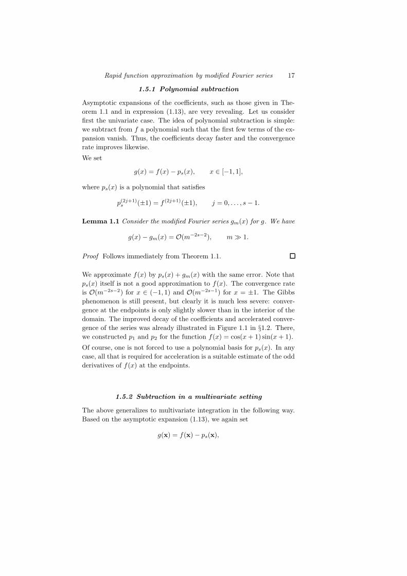
1.5.1 Polynomial subtraction

Asymptotic expansions of the coefficients, such as those given in The-

orem 1.1 and in expression (1.13), are very revealing. Let us consider

first the univariate case. The idea of polynomial subtraction is simple:

we subtract from f a polynomial such that the first few terms of the ex-

pansion vanish. Thus, the coefficients decay faster and the convergence

rate improves likewise.

We set

g(x) = f(x) − ps(x), x ∈ [−1, 1],

where ps(x) is a polynomial that satisfies

p(2j+1)s (±1) = f (2j+1)(±1), j = 0, . . . , s − 1.

Lemma 1.1 Consider the modified Fourier series gm(x) for g. We have

g(x) − gm(x) = O(m−2s−2), m ≫ 1.

Proof Follows immediately from Theorem 1.1.

We approximate f(x) by ps(x) + gm(x) with the same error. Note that

ps(x) itself is not a good approximation to f(x). The convergence rate

is O(m−2s−2) for x ∈ (−1, 1) and O(m−2s−1) for x = ±1. The Gibbs

phenomenon is still present, but clearly it is much less severe: conver-

gence at the endpoints is only slightly slower than in the interior of the

domain. The improved decay of the coefficients and accelerated conver-

gence of the series was already illustrated in Figure 1.1 in §1.2. There,

we constructed p1 and p2 for the function f(x) = cos(x + 1) sin(x + 1).

Of course, one is not forced to use a polynomial basis for ps(x). In any

case, all that is required for acceleration is a suitable estimate of the odd

derivatives of f(x) at the endpoints.

1.5.2 Subtraction in a multivariate setting

The above generalizes to multivariate integration in the following way.

Based on the asymptotic expansion (1.13), we again set

g(x) = f(x) − ps(x),


10 20 30 40 50

5

10

15

20

25

30

35

40

45

50−14

−12

−10

−8

−6

−4

−2

0

(a) No acceleration

10 20 30 40 50

5

10

15

20

25

30

35

40

45

50−14

−12

−10

−8

−6

−4

−2

0

(b) Subtraction of 1 boundary term

10 20 30 40 50

5

10

15

20

25

30

35

40

45

50−14

−12

−10

−8

−6

−4

−2

0

(c) Subtraction of 2 boundary terms

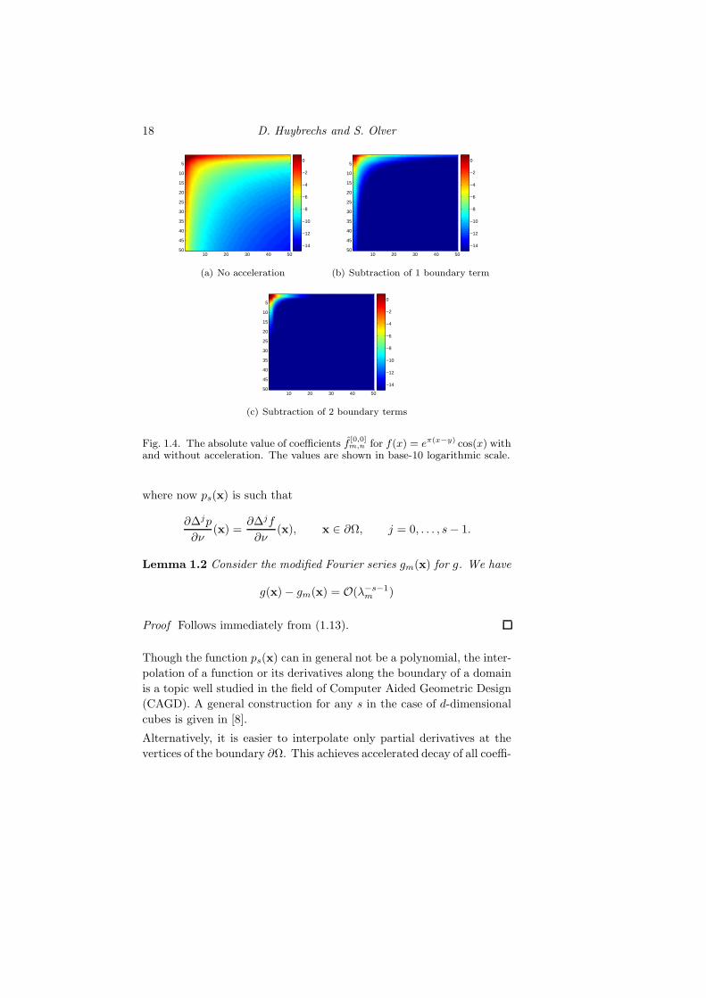
Fig. 1.4. The absolute value of coefficients f[0,0]m,n for f(x) = eπ(x−y) cos(x) with

and without acceleration. The values are shown in base-10 logarithmic scale.

where now ps(x) is such that

∂∆jp

∂ν(x) =

∂∆jf

∂ν(x), x ∈ ∂Ω, j = 0, . . . , s − 1.

Lemma 1.2 Consider the modified Fourier series gm(x) for g. We have

g(x) − gm(x) = O(λ−s−1m )

Proof Follows immediately from (1.13).

Though the function ps(x) can in general not be a polynomial, the inter-

polation of a function or its derivatives along the boundary of a domain

is a topic well studied in the field of Computer Aided Geometric Design

(CAGD). A general construction for any s in the case of d-dimensional

cubes is given in [8].

Alternatively, it is easier to interpolate only partial derivatives at the

vertices of the boundary ∂Ω. This achieves accelerated decay of all coeffi-


cients except for edge coefficients. The minimal set of partial derivatives

to interpolate depends on the shape of Ω.

We remark however that in boundary value problems, Neumann data

is precisely the sort of information that may be available. The use of

modified Fourier series in spectral methods for boundary value problems

was recently explored in [1]. It was found that modified Fourier series are

better behaved in this setting than Chebyshev expansions. In particular,

the condition number of the discretization matrix behaves as O(m2) for

modified Fourier series, but as O(m4) for Chebyshev expansions.

Figure 1.4 illustrates the size of the modified Fourier coefficients for

the case of the square Ω := [−1, 1] and the smooth function f(x) =

eπ(x−y) cos(x). The level curves roughly correspond to constant m2n2,

due to the O(m−2n−2) behaviour of the coefficients. The hyperbolic

cross derives from the hyperbolic shape of these curves. The hyper-

bolic cross is particularly interesting in higher dimension: one can show

that the number of coefficients larger than a given threshold grows only

logarithmically with dimension, rather than exponentially [8]. The ac-

celeration procedure in this two-dimensional example is very effective

indeed. For example, the number of elements larger than 10−5 in panel

(a) is 2, 113, in panel (b) it is 184 and in panel (c) only 58. In the latter

case, the coefficients behave as O(m−6n−6), for m, n ≫ 1.

1.6 Concluding remarks

At the beginning of this paper, we motivated the use of modified Fourier

series by comparing to classical Fourier series and Chebyshev expansions.

To summarize, we note the following advantages:

(i) The first m coefficients can be computed in O(m) operations.

(ii) Additional coefficients can be computed adaptively, with an O(1)

cost associated to each term.

(iii) The method of approximation generalizes in different directions:

to eigenfunctions of polyharmonic operators and to general do-

mains Ω including ellipses, cubes and triangles. (And, by ex-

tension, to any Ω that can be tessellated by these basic shapes.

For example, any polygon can be divided in a set of triangles,

and functions defined on a polygon can be approximated in each

triangle separately.)

(iv) Modified Fourier series are more stable in spectral methods than


Chebyshev expansions, exhibiting a typical O(m2) condition num-

ber of the discretization matrix rather than O(m4).

Compared to FFT for non-periodic functions, modified Fourier series

overcome the Gibbs phenomenon and yield pointwise convergence at the

boundary. These facts are even more true when convergence accelera-

tion is used. An alternative, and very effective, procedure for defeating

the Gibbs phenomenon in one dimension was also reviewed in [7]. The

described method achieves exponential accuracy in the reconstruction of

a non-periodic function f from its values in equidistant points, much like

FFT for periodic functions, by expanding the partial Fourier sum into a

set of Gegenbauer polynomials. The computations involved can become

unstable however if f has singularities close to the real axis [3]. Modified

Fourier series on the other hand, leaving generality aside, are guaran-

teed to be stable for all domains Ω: all coefficients are easily bounded

in terms of the maximum of |f | on Ω. Moreover, the techniques for

convergence acceleration are quite flexible, and we anticipate that the

degrees of freedom may be used in the future to produce numerically

stable algorithms in a variety of applications.

Bibliography

[1] Adcock, B. (2007). Spectral methods and modified Fourier series, TechnicalReport 2007/NA08, University of Cambridge.

[2] Babenko, K. (1960). Approximation of periodic functions of many variablesby trigonometric polynomials, Soviet Maths 1, 513–516.

[3] Boyd, J.P. (2005). Trouble with Gegenbauer reconstruction for defeatingGibbs’ phenomenon: Runge phenomenon in the diagonal limit of Gegen-bauer polynomial approximations, J. Comput. Phys. 204, 253–264.

[4] Cools, R. (1997). Constructing cubature formulae: The science behind theart, Acta Numer. 6, 1–54.

[5] Courant, R. and Hilbert, D. (1962). Methods of mathematical physics (WileyInterscience, New York).

[6] Davis, P. J. and Rabinowitz, P. (1984). Methods of numerical integra-tion, Computer Science and Applied Mathematics (Academic Press, NewYork).

[7] Gottlieb, D. and Shu, C.-W. (1997). On the Gibbs phenomenon and itsresolution, SIAM Rev. 39, 644–668.

[8] Huybrechs, D., Iserles, A. and Nørsett, S. P. (2007). From high oscillationto rapid approximation IV: Accelerating convergence, Technical ReportNA2007/07, University of Cambridge.

[9] Huybrechs, D. and Olver, S. (2008). Highly oscillatory quadrature, in HighlyOscillatory Problems: Computation, Theory and Applications, ed. B. En-gquist et al (Cambridge University Press, Cambridge).


[10] Iserles, A. and Nørsett, S. P. (2005). Efficient quadrature of highly oscilla-tory integrals using derivatives, Proc. R. Soc. Lond. A 461, 1383–1399.

[11] Iserles, A. and Nørsett, S. P. (2006). From high oscillation to rapid approx-imation I: Modified Fourier expansions, Technical Report 2006/NA05,University of Cambridge.

[12] Iserles, A. and Nørsett, S. P. (2006). From high oscillation to rapid approx-imation II: Expansions in polyharmonic eigenfunctions, Technical Report2006/NA07, University of Cambridge.

[13] Iserles, A. and Nørsett, S. P. (2007). From high oscillation to rapid ap-proximation III:Multivariate expansions, Technical Report 2007/NA01,University of Cambridge.

[14] Olver, S. (2007). On the convergence rate of a modified Fourier series,Technical Report 2007/NA02, University of Cambridge.

[15] Poschel, J. and Trubowitz, E. (1987). Inverse Spectral Theory (AcademicPress, Boston).

Rapid function approximation by modiﬁed Fourier seriesdaan/research/MFS.pdf · Rapid function...

Documents

Transcript of Rapid function approximation by modiﬁed Fourier seriesdaan/research/MFS.pdf · Rapid function...