· 16 random setting in the family of all geometric equations, F(p,x) = |p|+ < V ·p >, satisfying...
112
1 homogenization of the G-equation in random environments Panagiotis E. Souganidis University of Chicago
Transcript of · 16 random setting in the family of all geometric equations, F(p,x) = |p|+ < V ·p >, satisfying...
1
homogenization of the G-equation in random environments
Panagiotis E. SouganidisUniversity of Chicago
2
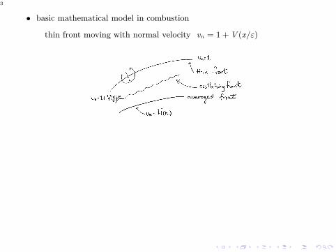
• basic mathematical model in combustion
thin front moving with normal velocity vn = 1 + V (x/ε)
3
• basic mathematical model in combustion
thin front moving with normal velocity vn = 1 + V (x/ε)
4
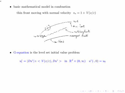
• basic mathematical model in combustion
thin front moving with normal velocity vn = 1 + V (x/ε)
• G-equation is the level set initial value problem
uεt = |Duε|+ < V (x/ε), Duε > in R
d × (0, ∞) uε(·, 0) = u0
5
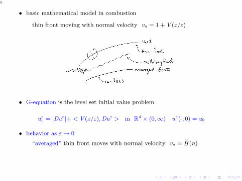
• basic mathematical model in combustion
thin front moving with normal velocity vn = 1 + V (x/ε)
• G-equation is the level set initial value problem
uεt = |Duε|+ < V (x/ε), Duε > in R
d × (0, ∞) uε(·, 0) = u0
• behavior as ε → 0
“averaged” thin front moves with normal velocity vn = H (n)
6
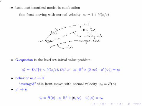
• basic mathematical model in combustion
thin front moving with normal velocity vn = 1 + V (x/ε)
• G-equation is the level set initial value problem
uεt = |Duε|+ < V (x/ε), Duε > in R
d × (0, ∞) uε(·, 0) = u0
• behavior as ε → 0
“averaged” thin front moves with normal velocity vn = H (n)
• uε → u
ut = H (u) in Rd × (0, ∞) u(·, 0) = u0
7
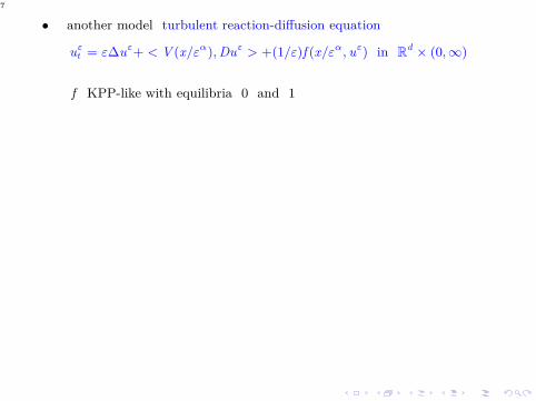
• another model turbulent reaction-diffusion equation
uεt = ε∆uε+ < V (x/εα), Duε > +(1/ε)f (x/εα, uε) in R
d × (0, ∞)
f KPP-like with equilibria 0 and 1
8
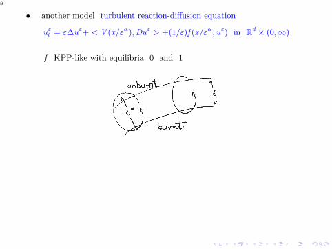
• another model turbulent reaction-diffusion equation
uεt = ε∆uε+ < V (x/εα), Duε > +(1/ε)f (x/εα, uε) in R
d × (0, ∞)
f KPP-like with equilibria 0 and 1
9
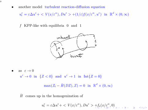
• another model turbulent reaction-diffusion equation
uεt = ε∆uε+ < V (x/εα), Duε > +(1/ε)f (x/εα, uε) in R
d × (0, ∞)
f KPP-like with equilibria 0 and 1
• as ε → 0
uε → 0 in Z < 0 and uε → 1 in IntZ = 0
max(Zt − H (DZ), Z) = 0 in Rd × (0, ∞)
H comes up in the homogenization of
uεt = ε∆uε+ < V (x/εα), Duε > +fu(x/εα, 0)
10
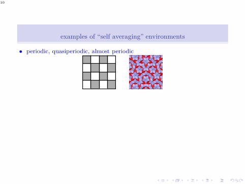
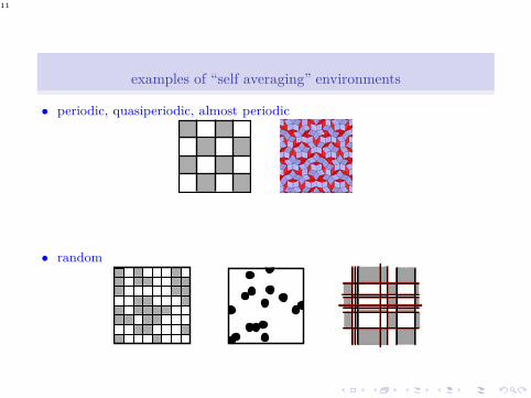
examples of “self averaging” environments
• periodic, quasiperiodic, almost periodic
11
examples of “self averaging” environments
• periodic, quasiperiodic, almost periodic
• random
12
some more random examples
13
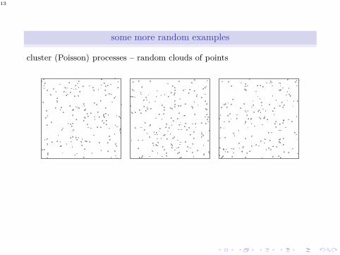
some more random examples
cluster (Poisson) processes – random clouds of points
14
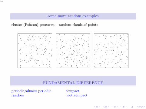
some more random examples
cluster (Poisson) processes – random clouds of points
FUNDAMENTAL DIFFERENCE
periodic/almost periodic compactrandom not compact
15
random setting
in the family of all geometric equations, F(p, x) = |p|+ < V · p >, satisfyingsome common uniform properties, like common Lip bounds, ... concentrateon a subfamily F(p, x, ω) appearing with some “frequency” described bythe fact that ω belongs to a probability space (Ω,F,P) such that
16
random setting
in the family of all geometric equations, F(p, x) = |p|+ < V · p >, satisfyingsome common uniform properties, like common Lip bounds, ... concentrateon a subfamily F(p, x, ω) appearing with some “frequency” described bythe fact that ω belongs to a probability space (Ω,F,P) such that
• if F(p, ·, ω) is in the family and we change position to y,then F(p, · + y, ω) is also in the family, i.e.,F(p, · + y, ω) = F(p, ·, τyω), and the frequency of appearance isindependent of the change of the location, i.e.,τy : Ω → Ω is measure preserving stationarity
17
random setting
in the family of all geometric equations, F(p, x) = |p|+ < V · p >, satisfyingsome common uniform properties, like common Lip bounds, ... concentrateon a subfamily F(p, x, ω) appearing with some “frequency” described bythe fact that ω belongs to a probability space (Ω,F,P) such that
• if F(p, ·, ω) is in the family and we change position to y,then F(p, · + y, ω) is also in the family, i.e.,F(p, · + y, ω) = F(p, ·, τyω), and the frequency of appearance isindependent of the change of the location, i.e.,τy : Ω → Ω is measure preserving stationarity
• under translations, the operators “repeat themselves”, i.e.,
if P(A) > 0, then P(∪y∈Rn τyA) = 1 ergodicity
18
a heuristic picture
• different equations have the same “frequency” no matter where they arelocated

19
a heuristic picture
• different equations have the same “frequency” no matter where they arelocated
20
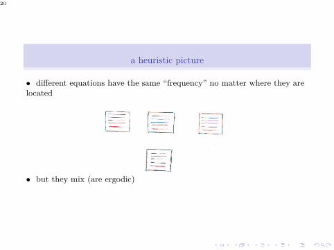
a heuristic picture
• different equations have the same “frequency” no matter where they arelocated
• but they mix (are ergodic)
21
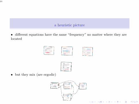
a heuristic picture
• different equations have the same “frequency” no matter where they arelocated
• but they mix (are ergodic)
22
the G-equation
uεt = |Duε|+ < V (x/ε), Duε > in R
d × (0, ∞)
23
the G-equation
uεt = |Duε|+ < V (x/ε), Duε > in R
d × (0, ∞)
• ‖V ‖ < 1 =⇒ problem is coercive
homogenization follows from results of
Lions, Papanicolaou, Varadhan (periodic), Ishii (almost periodic),Souganidis (stationary ergodic)
24
the G-equation
uεt = |Duε|+ < V (x/ε), Duε > in R
d × (0, ∞)
• ‖V ‖ < 1 =⇒ problem is coercive
homogenization follows from results of
Lions, Papanicolaou, Varadhan (periodic), Ishii (almost periodic),Souganidis (stationary ergodic)
• ‖V ‖ ≥ 1 =⇒ problem is not coercive
homogenization may not be possible
the uε’s may not converge locally uniformly
25
• an example
uεt = |Duε|+ < V (x/ε), Duε > in R
d × (0, ∞) and uε(·, 0) = u0
26
• an example
uεt = |Duε|+ < V (x/ε), Duε > in R
d × (0, ∞) and uε(·, 0) = u0
V = V (x) is 1-periodic and in Q1 = (−1/2, 1/2)d
V (x) = −10x if |x| < 1/6 and V (x) = 0 if |x| ≥ 1/3
27
• an example
uεt = |Duε|+ < V (x/ε), Duε > in R
d × (0, ∞) and uε(·, 0) = u0
V = V (x) is 1-periodic and in Q1 = (−1/2, 1/2)d
V (x) = −10x if |x| < 1/6 and V (x) = 0 if |x| ≥ 1/3
variational (control) representation formula ⇒ uǫ(x, t) = sup u0(X(x, t))
sup over all Lipschitz paths X with Xx(0) = x and
Xx(s) = V (Xx(s)) = α for controls |α| ≤ 1
28
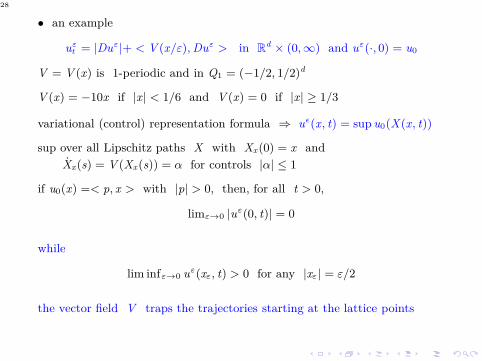
• an example
uεt = |Duε|+ < V (x/ε), Duε > in R
d × (0, ∞) and uε(·, 0) = u0
V = V (x) is 1-periodic and in Q1 = (−1/2, 1/2)d
V (x) = −10x if |x| < 1/6 and V (x) = 0 if |x| ≥ 1/3
variational (control) representation formula ⇒ uǫ(x, t) = sup u0(X(x, t))
sup over all Lipschitz paths X with Xx(0) = x and
Xx(s) = V (Xx(s)) = α for controls |α| ≤ 1
if u0(x) =< p, x > with |p| > 0, then, for all t > 0,
limε→0 |uε(0, t)| = 0
while
lim infε→0 uε(xε, t) > 0 for any |xε| = ε/2
the vector field V traps the trajectories starting at the lattice points
29
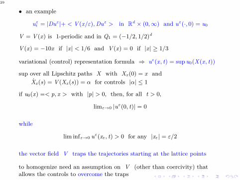
• an example
uεt = |Duε|+ < V (x/ε), Duε > in R
d × (0, ∞) and uε(·, 0) = u0
V = V (x) is 1-periodic and in Q1 = (−1/2, 1/2)d
V (x) = −10x if |x| < 1/6 and V (x) = 0 if |x| ≥ 1/3
variational (control) representation formula ⇒ uǫ(x, t) = sup u0(X(x, t))
sup over all Lipschitz paths X with Xx(0) = x and
Xx(s) = V (Xx(s)) = α for controls |α| ≤ 1
if u0(x) =< p, x > with |p| > 0, then, for all t > 0,
limε→0 |uε(0, t)| = 0
while
lim infε→0 uε(xε, t) > 0 for any |xε| = ε/2
the vector field V traps the trajectories starting at the lattice points
to homogenize need an assumption on V (other than coercivity) thatallows the controls to overcome the traps
30
the G-equation in the periodic setting
uεt = |Duε|+ < V (x/ε), Duε > in R
d × (0, ∞) and uε(·, 0) = u0
31
the G-equation in the periodic setting
uεt = |Duε|+ < V (x/ε), Duε > in R
d × (0, ∞) and uε(·, 0) = u0
V bounded, Lip. continuous, periodic and with “small divergence ”, i.e.
cI ‖ div V ‖Ld (Q) ≤ 1 (cI is the isoperimetric constant in the cube Q)
32
the G-equation in the periodic setting
uεt = |Duε|+ < V (x/ε), Duε > in R
d × (0, ∞) and uε(·, 0) = u0
V bounded, Lip. continuous, periodic and with “small divergence ”, i.e.
cI ‖ div V ‖Ld (Q) ≤ 1 (cI is the isoperimetric constant in the cube Q)
Theorem (convergence (Nolen, Cardaliaguet and Souganidis))
there exists a positively homogeneous (of degree one), Lipschitz continuous,convex, nonnegative H such that if ut = H (Du) = 0 in R
d × (0, ∞) andu(·, 0) = u0, then, as ε → 0, uε → u locally uniformly in R
d × (0, ∞)
special case by Xin and Yu
33
the G-equation in the periodic setting
uεt = |Duε|+ < V (x/ε), Duε > in R
d × (0, ∞) and uε(·, 0) = u0
V bounded, Lip. continuous, periodic and with “small divergence ”, i.e.
cI ‖ div V ‖Ld (Q) ≤ 1 (cI is the isoperimetric constant in the cube Q)
Theorem (convergence (Nolen, Cardaliaguet and Souganidis))
there exists a positively homogeneous (of degree one), Lipschitz continuous,convex, nonnegative H such that if ut = H (Du) = 0 in R
d × (0, ∞) andu(·, 0) = u0, then, as ε → 0, uε → u locally uniformly in R
d × (0, ∞)
special case by Xin and Yu
Theorem (enhancement (Nolen, Cardaliaguet and Souganidis))
(i) H (p) ≥ |p|(1 − cI ‖divV ‖Ld(Q))+ < E(V + x div V ), p >
(ii) if EV = 0 and div V = 0, then H (p) > |p| if and only if< V (x), p >= 0 for all x
34
the G-equation in random environments
uεt = |Duε|+ < V (x/ε), Duε > in R
d × (0, ∞) and uε(·, 0) = u0
35
the G-equation in random environments
uεt = |Duε|+ < V (x/ε), Duε > in R
d × (0, ∞) and uε(·, 0) = u0
V bounded, Lip. cont., stationary ergodic and EV = 0 and div V = 0
36
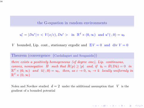
the G-equation in random environments
uεt = |Duε|+ < V (x/ε), Duε > in R
d × (0, ∞) and uε(·, 0) = u0
V bounded, Lip. cont., stationary ergodic and EV = 0 and div V = 0
Theorem (convergence (Cardaliaguet and Souganidis))
there exists a positively homogeneous (of degree one), Lip. continuous,convex, nonnegative H such that H (p) ≥ |p| and, if ut = H (Du) = 0 inR
d × (0, ∞) and u(·, 0) = u0, then, as ε → 0, uε → u locally uniformly inR
d × (0, ∞)
Nolen and Novikov studied d = 2 under the additional assumption that V is the
gradient of a bounded potential
37
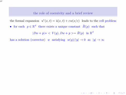
the role of coersivity and a brief review
the formal expansion uε(x, t) = u(x, t) + εw(x/ε) leads to the cell problem
• for each p ∈ Rd there exists a unique constant H (p) such that
|Dw + p|+ < V (y), Dw + p >= H (p) in Rd
has a solution (corrector) w satisfying w(y)/|y| → 0 as |y| → ∞
38
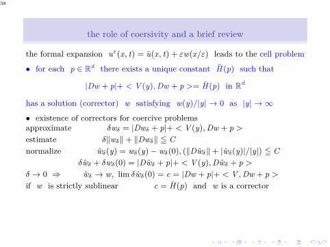
the role of coersivity and a brief review
the formal expansion uε(x, t) = u(x, t) + εw(x/ε) leads to the cell problem
• for each p ∈ Rd there exists a unique constant H (p) such that
|Dw + p|+ < V (y), Dw + p >= H (p) in Rd
has a solution (corrector) w satisfying w(y)/|y| → 0 as |y| → ∞
• existence of correctors for coercive problemsapproximate δwδ = |Dwδ + p|+ < V (y), Dw + p >
estimate δ‖wδ‖ + ‖Dwδ‖ ≦ C
normalize wδ(y) = wδ(y) − wδ(0), (‖Dwδ‖ + |wδ(y)|/|y|) ≦ C
δwδ + δwδ(0) = |Dwδ + p|+ < V (y), Dwδ + p >
δ → 0 ⇒ wδ → w, lim δwδ(0) = c = |Dw + p|+ < V , Dw + p >
if w is strictly sublinear c = H (p) and w is a corrector
39
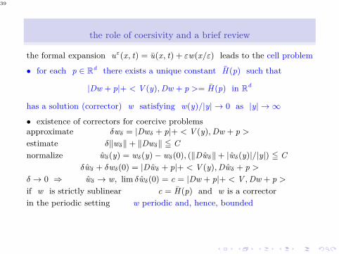
the role of coersivity and a brief review
the formal expansion uε(x, t) = u(x, t) + εw(x/ε) leads to the cell problem
• for each p ∈ Rd there exists a unique constant H (p) such that
|Dw + p|+ < V (y), Dw + p >= H (p) in Rd
has a solution (corrector) w satisfying w(y)/|y| → 0 as |y| → ∞
• existence of correctors for coercive problemsapproximate δwδ = |Dwδ + p|+ < V (y), Dw + p >
estimate δ‖wδ‖ + ‖Dwδ‖ ≦ C
normalize wδ(y) = wδ(y) − wδ(0), (‖Dwδ‖ + |wδ(y)|/|y|) ≦ C
δwδ + δwδ(0) = |Dwδ + p|+ < V (y), Dwδ + p >
δ → 0 ⇒ wδ → w, lim δwδ(0) = c = |Dw + p|+ < V , Dw + p >
if w is strictly sublinear c = H (p) and w is a corrector
in the periodic setting w periodic and, hence, bounded
40
the role of coersivity and a brief review
the formal expansion uε(x, t) = u(x, t) + εw(x/ε) leads to the cell problem
• for each p ∈ Rd there exists a unique constant H (p) such that
|Dw + p|+ < V (y), Dw + p >= H (p) in Rd
has a solution (corrector) w satisfying w(y)/|y| → 0 as |y| → ∞
• existence of correctors for coercive problemsapproximate δwδ = |Dwδ + p|+ < V (y), Dw + p >
estimate δ‖wδ‖ + ‖Dwδ‖ ≦ C
normalize wδ(y) = wδ(y) − wδ(0), (‖Dwδ‖ + |wδ(y)|/|y|) ≦ C
δwδ + δwδ(0) = |Dwδ + p|+ < V (y), Dwδ + p >
δ → 0 ⇒ wδ → w, lim δwδ(0) = c = |Dw + p|+ < V , Dw + p >
if w is strictly sublinear c = H (p) and w is a corrector
in the periodic setting w periodic and, hence, bounded
• strict sublinearity is a problem in stationary environments(counterexamples)
• no gradient bounds in noncoercive settings

41
remarks about the cell problem

42
remarks about the cell problem
approximate cell problem
δwδ = H (Dwδ + p, y) = |Dwδ + p|+ < V , Dwδ + p >
enough to prove δwδ → H uniformly in balls of radious 1/δ

43
remarks about the cell problem
approximate cell problem
δwδ = H (Dwδ + p, y) = |Dwδ + p|+ < V , Dwδ + p >
enough to prove δwδ → H uniformly in balls of radious 1/δ
• it is the best one can hope
44
remarks about the cell problem
approximate cell problem
δwδ = H (Dwδ + p, y) = |Dwδ + p|+ < V , Dwδ + p >
enough to prove δwδ → H uniformly in balls of radious 1/δ
• it is the best one can hope
wδ(x) = δwδ(x/δ) solves wδ = H (Dwδ + p, x/δ) in Rd
if the problem homogenizes, then the wδ’s converge locally uniformly to w
solving w = H (Dw + p) in Rd and, hence, w = H (p)
45
remarks about the cell problem
approximate cell problem
δwδ = H (Dwδ + p, y) = |Dwδ + p|+ < V , Dwδ + p >
enough to prove δwδ → H uniformly in balls of radious 1/δ
• it is the best one can hope
wδ(x) = δwδ(x/δ) solves wδ = H (Dwδ + p, x/δ) in Rd
if the problem homogenizes, then the wδ’s converge locally uniformly to w
solving w = H (Dw + p) in Rd and, hence, w = H (p)
• δwδ’s in balls of radius 1/δ ⇒ H is unique
46
remarks about the cell problem
approximate cell problem
δwδ = H (Dwδ + p, y) = |Dwδ + p|+ < V , Dwδ + p >
enough to prove δwδ → H uniformly in balls of radious 1/δ
• it is the best one can hope
wδ(x) = δwδ(x/δ) solves wδ = H (Dwδ + p, x/δ) in Rd
if the problem homogenizes, then the wδ’s converge locally uniformly to w
solving w = H (Dw + p) in Rd and, hence, w = H (p)
• δwδ’s in balls of radius 1/δ ⇒ H is unique
in periodic environments above convergence is equivalent to uniform andfollows if appropriate estimates are available
47
remarks about the cell problem
approximate cell problem
δwδ = H (Dwδ + p, y) = |Dwδ + p|+ < V , Dwδ + p >
enough to prove δwδ → H uniformly in balls of radious 1/δ
• it is the best one can hope
wδ(x) = δwδ(x/δ) solves wδ = H (Dwδ + p, x/δ) in Rd
if the problem homogenizes, then the wδ’s converge locally uniformly to w
solving w = H (Dw + p) in Rd and, hence, w = H (p)
• δwδ’s in balls of radius 1/δ ⇒ H is unique
in periodic environments above convergence is equivalent to uniform andfollows if appropriate estimates are available
in random media is not known how to obtain it without proving firsthomogenization – the problem is not luck of estimates but the luck ofcompactness

48
noncoercive periodic G-equation
49
noncoercive periodic G-equation
δwδ = |Dwδ + p|+ < V (y), Dwδ + p >
the Lipschitz bounded is replaced by
50
noncoercive periodic G-equation
δwδ = |Dwδ + p|+ < V (y), Dwδ + p >
the Lipschitz bounded is replaced by
• osc(δwδ) ≤ Cδ for some C = C (d, |p|)
51
noncoercive periodic G-equation
δwδ = |Dwδ + p|+ < V (y), Dwδ + p >
the Lipschitz bounded is replaced by
• osc(δwδ) ≤ Cδ for some C = C (d, |p|)
the key steps are
• if, for some θ ∈ (inf δwδ, sup δwδ), |δwδ < θ ∩ Q| < 1/2, then
δwδ ≥ θ − Cδ in Q
• if, for some θ ∈ (inf δwδ, sup δwδ), |δwδ > θ ∩ Q| > 1/2, then
δwδ ≤ θ + Cδ in Q
52
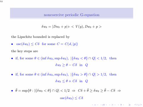
noncoercive periodic G-equation
δwδ = |Dwδ + p|+ < V (y), Dwδ + p >
the Lipschitz bounded is replaced by
• osc(δwδ) ≤ Cδ for some C = C (d, |p|)
the key steps are
• if, for some θ ∈ (inf δwδ, sup δwδ), |δwδ < θ ∩ Q| < 1/2, then
δwδ ≥ θ − Cδ in Q
• if, for some θ ∈ (inf δwδ, sup δwδ), |δwδ > θ ∩ Q| > 1/2, then
δwδ ≤ θ + Cδ in Q
• θ = supθ : |δwδ < θ ∩ Q| < 1/2 ⇒ Cδ + θ ≥ δwδ ≥ θ − Cδ ⇒
osc(δwδ) ≤ Cδ
53
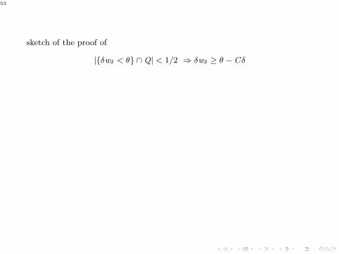
sketch of the proof of
|δwδ < θ ∩ Q| < 1/2 ⇒ δwδ ≥ θ − Cδ
54
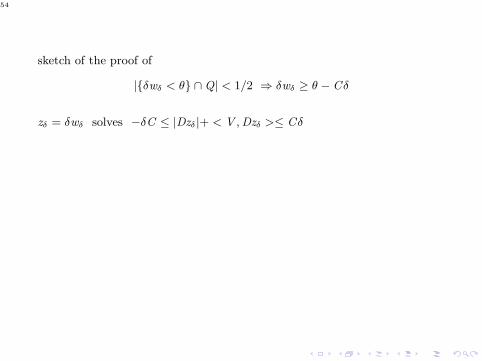
sketch of the proof of
|δwδ < θ ∩ Q| < 1/2 ⇒ δwδ ≥ θ − Cδ
zδ = δwδ solves −δC ≤ |Dzδ |+ < V , Dzδ >≤ Cδ
55
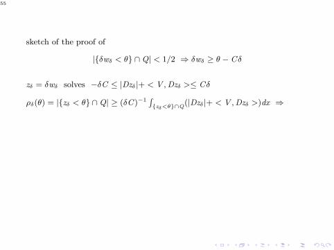
sketch of the proof of
|δwδ < θ ∩ Q| < 1/2 ⇒ δwδ ≥ θ − Cδ
zδ = δwδ solves −δC ≤ |Dzδ |+ < V , Dzδ >≤ Cδ
ρδ(θ) = |zδ < θ ∩ Q| ≥ (δC )−1´
zδ<θ∩Q(|Dzδ|+ < V , Dzδ >)dx ⇒
56
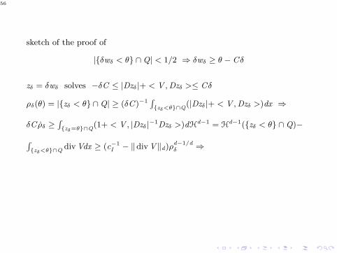
sketch of the proof of
|δwδ < θ ∩ Q| < 1/2 ⇒ δwδ ≥ θ − Cδ
zδ = δwδ solves −δC ≤ |Dzδ |+ < V , Dzδ >≤ Cδ
ρδ(θ) = |zδ < θ ∩ Q| ≥ (δC )−1´
zδ<θ∩Q(|Dzδ|+ < V , Dzδ >)dx ⇒
δC ρδ ≥´
zδ=θ∩Q(1+ < V , |Dzδ |−1Dzδ >)dHd−1 = H
d−1(zδ < θ ∩ Q)−
´
zδ<θ∩Qdiv Vdx ≥ (c−1
I − ‖ div V ‖d)ρd−1/d
δ ⇒
57
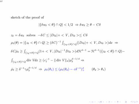
sketch of the proof of
|δwδ < θ ∩ Q| < 1/2 ⇒ δwδ ≥ θ − Cδ
zδ = δwδ solves −δC ≤ |Dzδ |+ < V , Dzδ >≤ Cδ
ρδ(θ) = |zδ < θ ∩ Q| ≥ (δC )−1´
zδ<θ∩Q(|Dzδ|+ < V , Dzδ >)dx ⇒
δC ρδ ≥´
zδ=θ∩Q(1+ < V , |Dzδ |−1Dzδ >)dHd−1 = H
d−1(zδ < θ ∩ Q)−
´
zδ<θ∩Qdiv Vdx ≥ (c−1
I − ‖ div V ‖d)ρd−1/d
δ ⇒
ρδ ≥ δ−1γρd−1/d
δ ⇒ ρδ(θ1) ≤ (ρδ(θ2) − cδ−1)d+ (θ2 > θ1)
58
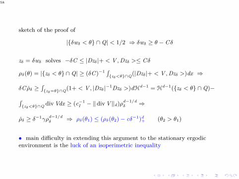
sketch of the proof of
|δwδ < θ ∩ Q| < 1/2 ⇒ δwδ ≥ θ − Cδ
zδ = δwδ solves −δC ≤ |Dzδ |+ < V , Dzδ >≤ Cδ
ρδ(θ) = |zδ < θ ∩ Q| ≥ (δC )−1´
zδ<θ∩Q(|Dzδ|+ < V , Dzδ >)dx ⇒
δC ρδ ≥´
zδ=θ∩Q(1+ < V , |Dzδ |−1Dzδ >)dHd−1 = H
d−1(zδ < θ ∩ Q)−
´
zδ<θ∩Qdiv Vdx ≥ (c−1
I − ‖ div V ‖d)ρd−1/d
δ ⇒
ρδ ≥ δ−1γρd−1/d
δ ⇒ ρδ(θ1) ≤ (ρδ(θ2) − cδ−1)d+ (θ2 > θ1)
• main difficulty in extending this argument to the stationary ergodicenvironment is the luck of an isoperimetric inequality
59
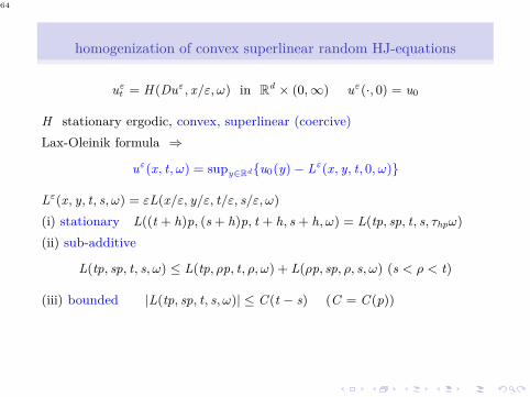
homogenization of convex superlinear random HJ-equations
uεt = H (Duε, x/ε, ω) in R
d × (0, ∞) uε(·, 0) = u0
H stationary ergodic, convex, superlinear (coercive)
60
homogenization of convex superlinear random HJ-equations
uεt = H (Duε, x/ε, ω) in R
d × (0, ∞) uε(·, 0) = u0
H stationary ergodic, convex, superlinear (coercive)
Lax-Oleinik formula ⇒
uε(x, t, ω) = supy∈Rd u0(y) − Lε(x, y, t, 0, ω)
61
homogenization of convex superlinear random HJ-equations
uεt = H (Duε, x/ε, ω) in R
d × (0, ∞) uε(·, 0) = u0
H stationary ergodic, convex, superlinear (coercive)
Lax-Oleinik formula ⇒
uε(x, t, ω) = supy∈Rd u0(y) − Lε(x, y, t, 0, ω)
Lε(x, y, t, s, ω) = εL(x/ε, y/ε, t/ε, s/ε, ω)
62
homogenization of convex superlinear random HJ-equations
uεt = H (Duε, x/ε, ω) in R
d × (0, ∞) uε(·, 0) = u0
H stationary ergodic, convex, superlinear (coercive)
Lax-Oleinik formula ⇒
uε(x, t, ω) = supy∈Rd u0(y) − Lε(x, y, t, 0, ω)
Lε(x, y, t, s, ω) = εL(x/ε, y/ε, t/ε, s/ε, ω)
(i) stationary L((t + h)p, (s + h)p, t + h, s + h, ω) = L(tp, sp, t, s, τhpω)
63
homogenization of convex superlinear random HJ-equations
uεt = H (Duε, x/ε, ω) in R
d × (0, ∞) uε(·, 0) = u0
H stationary ergodic, convex, superlinear (coercive)
Lax-Oleinik formula ⇒
uε(x, t, ω) = supy∈Rd u0(y) − Lε(x, y, t, 0, ω)
Lε(x, y, t, s, ω) = εL(x/ε, y/ε, t/ε, s/ε, ω)
(i) stationary L((t + h)p, (s + h)p, t + h, s + h, ω) = L(tp, sp, t, s, τhpω)
(ii) sub-additive
L(tp, sp, t, s, ω) ≤ L(tp, ρp, t, ρ, ω) + L(ρp, sp, ρ, s, ω) (s < ρ < t)
64
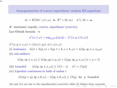
homogenization of convex superlinear random HJ-equations
uεt = H (Duε, x/ε, ω) in R
d × (0, ∞) uε(·, 0) = u0
H stationary ergodic, convex, superlinear (coercive)
Lax-Oleinik formula ⇒
uε(x, t, ω) = supy∈Rd u0(y) − Lε(x, y, t, 0, ω)
Lε(x, y, t, s, ω) = εL(x/ε, y/ε, t/ε, s/ε, ω)
(i) stationary L((t + h)p, (s + h)p, t + h, s + h, ω) = L(tp, sp, t, s, τhpω)
(ii) sub-additive
L(tp, sp, t, s, ω) ≤ L(tp, ρp, t, ρ, ω) + L(ρp, sp, ρ, s, ω) (s < ρ < t)
(iii) bounded |L(tp, sp, t, s, ω)| ≤ C (t − s) (C = C (p))
65
homogenization of convex superlinear random HJ-equations
uεt = H (Duε, x/ε, ω) in R
d × (0, ∞) uε(·, 0) = u0
H stationary ergodic, convex, superlinear (coercive)
Lax-Oleinik formula ⇒
uε(x, t, ω) = supy∈Rd u0(y) − Lε(x, y, t, 0, ω)
Lε(x, y, t, s, ω) = εL(x/ε, y/ε, t/ε, s/ε, ω)
(i) stationary L((t + h)p, (s + h)p, t + h, s + h, ω) = L(tp, sp, t, s, τhpω)
(ii) sub-additive
L(tp, sp, t, s, ω) ≤ L(tp, ρp, t, ρ, ω) + L(ρp, sp, ρ, s, ω) (s < ρ < t)
(iii) bounded |L(tp, sp, t, s, ω)| ≤ C (t − s) (C = C (p))
(iv) Lipschitz continuous in balls of radius t
|L(t(p + q), tp, t, 0, ω) − L(tp, t, 0, ω)| ≤ Ct|q| for p bounded
(iii) and (iv) are due to the superlinearity/coercivity while (ii) follows form convexity
66
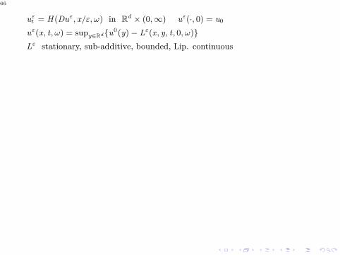
uεt = H (Duε, x/ε, ω) in R
d × (0, ∞) uε(·, 0) = u0
uε(x, t, ω) = supy∈Rd u0(y) − Lε(x, y, t, 0, ω)
Lε stationary, sub-additive, bounded, Lip. continuous
67
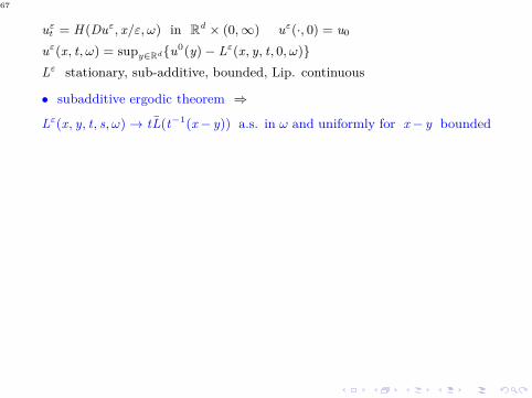
uεt = H (Duε, x/ε, ω) in R
d × (0, ∞) uε(·, 0) = u0
uε(x, t, ω) = supy∈Rd u0(y) − Lε(x, y, t, 0, ω)
Lε stationary, sub-additive, bounded, Lip. continuous
• subadditive ergodic theorem ⇒
Lε(x, y, t, s, ω) → tL(t−1(x − y)) a.s. in ω and uniformly for x − y bounded
68
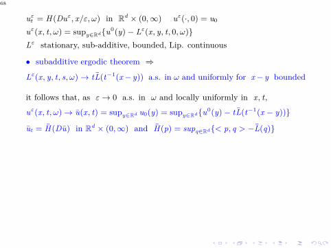
uεt = H (Duε, x/ε, ω) in R
d × (0, ∞) uε(·, 0) = u0
uε(x, t, ω) = supy∈Rd u0(y) − Lε(x, y, t, 0, ω)
Lε stationary, sub-additive, bounded, Lip. continuous
• subadditive ergodic theorem ⇒
Lε(x, y, t, s, ω) → tL(t−1(x − y)) a.s. in ω and uniformly for x − y bounded
it follows that, as ε → 0 a.s. in ω and locally uniformly in x, t,
uε(x, t, ω) → u(x, t) = supy∈Rd u0(y) = supy∈Rd u0(y) − tL(t−1(x − y))
ut = H (Du) in Rd × (0, ∞) and H (p) = supq∈Rd < p, q > −L(q)
69
uεt = H (Duε, x/ε, ω) in R
d × (0, ∞) uε(·, 0) = u0
uε(x, t, ω) = supy∈Rd u0(y) − Lε(x, y, t, 0, ω)
Lε stationary, sub-additive, bounded, Lip. continuous
• subadditive ergodic theorem ⇒
Lε(x, y, t, s, ω) → tL(t−1(x − y)) a.s. in ω and uniformly for x − y bounded
it follows that, as ε → 0 a.s. in ω and locally uniformly in x, t,
uε(x, t, ω) → u(x, t) = supy∈Rd u0(y) = supy∈Rd u0(y) − tL(t−1(x − y))
ut = H (Du) in Rd × (0, ∞) and H (p) = supq∈Rd < p, q > −L(q)
main difficulty for the G-equation is the lack of coercivity
70
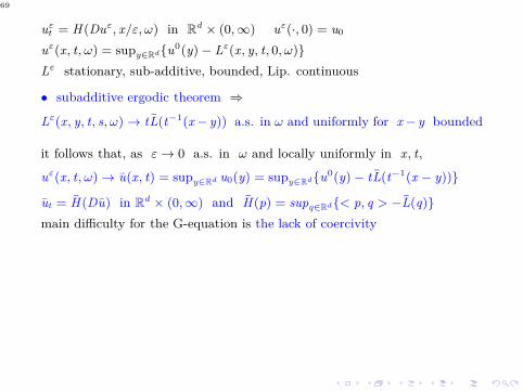
uεt = H (Duε, x/ε, ω) in R
d × (0, ∞) uε(·, 0) = u0
uε(x, t, ω) = supy∈Rd u0(y) − Lε(x, y, t, 0, ω)
Lε stationary, sub-additive, bounded, Lip. continuous
• subadditive ergodic theorem ⇒
Lε(x, y, t, s, ω) → tL(t−1(x − y)) a.s. in ω and uniformly for x − y bounded
it follows that, as ε → 0 a.s. in ω and locally uniformly in x, t,
uε(x, t, ω) → u(x, t) = supy∈Rd u0(y) = supy∈Rd u0(y) − tL(t−1(x − y))
ut = H (Du) in Rd × (0, ∞) and H (p) = supq∈Rd < p, q > −L(q)
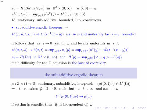
main difficulty for the G-equation is the lack of coercivity
the sub-additive ergodic theorem
µ : B × Ω → R stationary, subadditive, integrable (µ((0, 1), ·) ∈ L1(Ω))
⇒ there exists µ : Ω → R such that, as t → ∞ and a.s. in ω,
t−1µ((0, t), ω) → µ(ω)
if setting is ergodic, then µ is independent of ω
71
noncoercive G-equation in stationary random media
72
noncoercive G-equation in stationary random media
uεt = |Duε|+ < V (x/ε), Duε > in R
d × (0, ∞) uε(·, 0) = u0
73
noncoercive G-equation in stationary random media
uεt = |Duε|+ < V (x/ε), Duε > in R
d × (0, ∞) uε(·, 0) = u0
Lax-Oleinik formula ⇒
uε(x, t, ω) = supα∈A u0(Xα,ε,ωx (t)) = supy∈Rε(x,t,ω) u0(y)
= supy∈Rd u0(y) − Lε(x, y, t, ω)
74
noncoercive G-equation in stationary random media
uεt = |Duε|+ < V (x/ε), Duε > in R
d × (0, ∞) uε(·, 0) = u0
Lax-Oleinik formula ⇒
uε(x, t, ω) = supα∈A u0(Xα,ε,ωx (t)) = supy∈Rε(x,t,ω) u0(y)
= supy∈Rd u0(y) − Lε(x, y, t, ω)
A = α : L∞((0, ∞);Rd) with ‖α‖ ≤ 1
Xα,εx (s) = V (Xα,ε
x (s)/ε, ω) + α(s) Xα,εx (0) = x
75
noncoercive G-equation in stationary random media
uεt = |Duε|+ < V (x/ε), Duε > in R
d × (0, ∞) uε(·, 0) = u0
Lax-Oleinik formula ⇒
uε(x, t, ω) = supα∈A u0(Xα,ε,ωx (t)) = supy∈Rε(x,t,ω) u0(y)
= supy∈Rd u0(y) − Lε(x, y, t, ω)
A = α : L∞((0, ∞);Rd) with ‖α‖ ≤ 1
Xα,εx (s) = V (Xα,ε
x (s)/ε, ω) + α(s) Xα,εx (0) = x
Rε(x, t, ω) the reachable set of x at time t
76
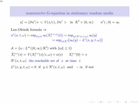
noncoercive G-equation in stationary random media
uεt = |Duε|+ < V (x/ε), Duε > in R
d × (0, ∞) uε(·, 0) = u0
Lax-Oleinik formula ⇒
uε(x, t, ω) = supα∈A u0(Xα,ε,ωx (t)) = supy∈Rε(x,t,ω) u0(y)
= supy∈Rd u0(y) − Lε(x, y, t, ω)
A = α : L∞((0, ∞);Rd) with ‖α‖ ≤ 1
Xα,εx (s) = V (Xα,ε
x (s)/ε, ω) + α(s) Xα,εx (0) = x
Rε(x, t, ω) the reachable set of x at time t
Lε(x, y, t, ω) = 0 if y ∈ Rε(x, t, ω) and − ∞ if not
77
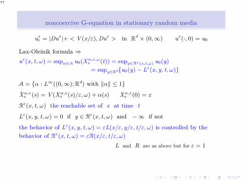
noncoercive G-equation in stationary random media
uεt = |Duε|+ < V (x/ε), Duε > in R
d × (0, ∞) uε(·, 0) = u0
Lax-Oleinik formula ⇒
uε(x, t, ω) = supα∈A u0(Xα,ε,ωx (t)) = supy∈Rε(x,t,ω) u0(y)
= supy∈Rd u0(y) − Lε(x, y, t, ω)
A = α : L∞((0, ∞);Rd) with ‖α‖ ≤ 1
Xα,εx (s) = V (Xα,ε
x (s)/ε, ω) + α(s) Xα,εx (0) = x
Rε(x, t, ω) the reachable set of x at time t
Lε(x, y, t, ω) = 0 if y ∈ Rε(x, t, ω) and − ∞ if not
the behavior of Lε(x, y, t, ω) = εL(x/ε, y/ε, t/ε, ω) is controlled by the
behavior of Rε(x, t, ω) = εR(x/ε, t/ε, ω)
L and R are as above but for ε = 1
78
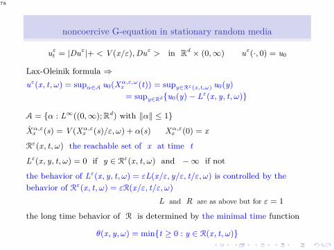
noncoercive G-equation in stationary random media
uεt = |Duε|+ < V (x/ε), Duε > in R
d × (0, ∞) uε(·, 0) = u0
Lax-Oleinik formula ⇒
uε(x, t, ω) = supα∈A u0(Xα,ε,ωx (t)) = supy∈Rε(x,t,ω) u0(y)
= supy∈Rd u0(y) − Lε(x, y, t, ω)
A = α : L∞((0, ∞);Rd) with ‖α‖ ≤ 1
Xα,εx (s) = V (Xα,ε
x (s)/ε, ω) + α(s) Xα,εx (0) = x
Rε(x, t, ω) the reachable set of x at time t
Lε(x, y, t, ω) = 0 if y ∈ Rε(x, t, ω) and − ∞ if not
the behavior of Lε(x, y, t, ω) = εL(x/ε, y/ε, t/ε, ω) is controlled by the
behavior of Rε(x, t, ω) = εR(x/ε, t/ε, ω)
L and R are as above but for ε = 1
the long time behavior of R is determined by the minimal time function
θ(x, y, ω) = mint ≥ 0 : y ∈ R(x, t, ω)
79
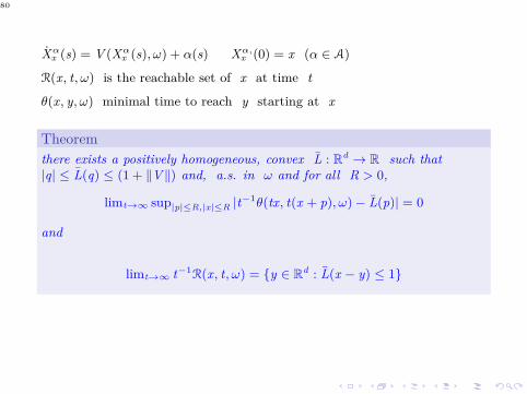
Xαx (s) = V (Xα
x (s), ω) + α(s) Xα,x (0) = x (α ∈ A)
R(x, t, ω) is the reachable set of x at time t
θ(x, y, ω) minimal time to reach y starting at x
80
Xαx (s) = V (Xα
x (s), ω) + α(s) Xα,x (0) = x (α ∈ A)
R(x, t, ω) is the reachable set of x at time t
θ(x, y, ω) minimal time to reach y starting at x
Theorem
there exists a positively homogeneous, convex L : Rd → R such that|q| ≤ L(q) ≤ (1 + ‖V ‖) and, a.s. in ω and for all R > 0,
limt→∞ sup|p|≤R,|x|≤R |t−1θ(tx, t(x + p), ω) − L(p)| = 0
and
limt→∞ t−1R(x, t, ω) = y ∈ R
d : L(x − y) ≤ 1
81
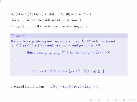
Xαx (s) = V (Xα
x (s), ω) + α(s) Xα,x (0) = x (α ∈ A)
R(x, t, ω) is the reachable set of x at time t
θ(x, y, ω) minimal time to reach y starting at x
Theorem
there exists a positively homogeneous, convex L : Rd → R such that|q| ≤ L(q) ≤ (1 + ‖V ‖) and, a.s. in ω and for all R > 0,
limt→∞ sup|p|≤R,|x|≤R |t−1θ(tx, t(x + p), ω) − L(p)| = 0
and
limt→∞ t−1R(x, t, ω) = y ∈ R
d : L(x − y) ≤ 1
averaged Hamiltonian H (p) = sup< p, q >: L(q) = 1
82
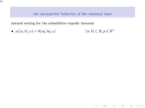
the asymptotic behavior of the minimal time
natural setting for the subadditive ergodic theorem
• µ((a, b), ω) = θ(aq, bq, ω) (a, b) ⊂ R, p ∈ Rd
83
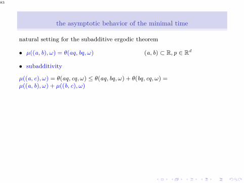
the asymptotic behavior of the minimal time
natural setting for the subadditive ergodic theorem
• µ((a, b), ω) = θ(aq, bq, ω) (a, b) ⊂ R, p ∈ Rd
• subadditivity
µ((a, c), ω) = θ(aq, cq, ω) ≤ θ(aq, bq, ω) + θ(bq, cq, ω) =µ((a, b), ω) + µ((b, c), ω)
84
the asymptotic behavior of the minimal time
natural setting for the subadditive ergodic theorem
• µ((a, b), ω) = θ(aq, bq, ω) (a, b) ⊂ R, p ∈ Rd
• subadditivity
µ((a, c), ω) = θ(aq, cq, ω) ≤ θ(aq, bq, ω) + θ(bq, cq, ω) =µ((a, b), ω) + µ((b, c), ω)
• stationarity
µ(c + (a, b), ω) = θ((a + c)q, (b + c)q, ω) = θ((aq, bq, τcqω) =µ((a, b), τcqω)
85
the asymptotic behavior of the minimal time
natural setting for the subadditive ergodic theorem
• µ((a, b), ω) = θ(aq, bq, ω) (a, b) ⊂ R, p ∈ Rd
• subadditivity
µ((a, c), ω) = θ(aq, cq, ω) ≤ θ(aq, bq, ω) + θ(bq, cq, ω) =µ((a, b), ω) + µ((b, c), ω)
• stationarity
µ(c + (a, b), ω) = θ((a + c)q, (b + c)q, ω) = θ((aq, bq, τcqω) =µ((a, b), τcqω)
• L1– bound there is a nontrivial difficulty here
for all ε ∈ (0, ε0) and a.s. in ω, there exists T (ω, ε) > 0 such that
θ(x, y, ω) ≤ T (ω, ε) + ε|x| + (1 + ε)|y − x| for all x, y ∈ Rd
not known whether T (·, ε) ∈ L1(Ω)
cannot use subadditive ergodic thm
86
new strategy
for each q ∈ Rd with |q| < 1 find α ∈ A so that the soln X0,0,α,ω of
X0,0,α,ω(s) = V (X0,0,α,ω(s), ω) + α(s) with X0,0,α,ω(0) = 0
(i) has, a.s. in ω and as t → ∞, an average t−1X0,0,α,ω(t) close to q
(ii) the subadditive ergodic thm can be applied to the minimal timeθ(X0,0,α,ω(s), X0,0,α,ω(t)) yielding a random variable γ such that, ast → ∞ and a.s. in ω, t−1θ(0, X0,0,α,ω(t), ω) → γ(ω)
87
new strategy
for each q ∈ Rd with |q| < 1 find α ∈ A so that the soln X0,0,α,ω of
X0,0,α,ω(s) = V (X0,0,α,ω(s), ω) + α(s) with X0,0,α,ω(0) = 0
(i) has, a.s. in ω and as t → ∞, an average t−1X0,0,α,ω(t) close to q
(ii) the subadditive ergodic thm can be applied to the minimal timeθ(X0,0,α,ω(s), X0,0,α,ω(t)) yielding a random variable γ such that, ast → ∞ and a.s. in ω, t−1θ(0, X0,0,α,ω(t), ω) → γ(ω)
fix q, α; write Xs for X0,0,α,ω(s); recall |Xs| ≤ C (1 + | V ‖)t
subadditivity, reachability estimate ⇒
θ(0, tq, ω) ≤ θ(0, Xt , ω) + θ(Xt, tq, ω) ≤
θ(0, Xt, ω) + T (ω, ε) + ε|Xt| + (1 + ε)|Xt − tq|
88
new strategy
for each q ∈ Rd with |q| < 1 find α ∈ A so that the soln X0,0,α,ω of
X0,0,α,ω(s) = V (X0,0,α,ω(s), ω) + α(s) with X0,0,α,ω(0) = 0
(i) has, a.s. in ω and as t → ∞, an average t−1X0,0,α,ω(t) close to q
(ii) the subadditive ergodic thm can be applied to the minimal timeθ(X0,0,α,ω(s), X0,0,α,ω(t)) yielding a random variable γ such that, ast → ∞ and a.s. in ω, t−1θ(0, X0,0,α,ω(t), ω) → γ(ω)
fix q, α; write Xs for X0,0,α,ω(s); recall |Xs| ≤ C (1 + | V ‖)t
subadditivity, reachability estimate ⇒
θ(0, tq, ω) ≤ θ(0, Xt , ω) + θ(Xt, tq, ω) ≤
θ(0, Xt, ω) + T (ω, ε) + ε|Xt| + (1 + ε)|Xt − tq|
properties of Xt ⇒ lim supt→∞ t−1θ(0, tq, ω) ≤ γ(ω) + εC
89
new strategy
for each q ∈ Rd with |q| < 1 find α ∈ A so that the soln X0,0,α,ω of
X0,0,α,ω(s) = V (X0,0,α,ω(s), ω) + α(s) with X0,0,α,ω(0) = 0
(i) has, a.s. in ω and as t → ∞, an average t−1X0,0,α,ω(t) close to q
(ii) the subadditive ergodic thm can be applied to the minimal timeθ(X0,0,α,ω(s), X0,0,α,ω(t)) yielding a random variable γ such that, ast → ∞ and a.s. in ω, t−1θ(0, X0,0,α,ω(t), ω) → γ(ω)
fix q, α; write Xs for X0,0,α,ω(s); recall |Xs| ≤ C (1 + | V ‖)t
subadditivity, reachability estimate ⇒
θ(0, tq, ω) ≤ θ(0, Xt , ω) + θ(Xt, tq, ω) ≤
θ(0, Xt, ω) + T (ω, ε) + ε|Xt| + (1 + ε)|Xt − tq|
properties of Xt ⇒ lim supt→∞ t−1θ(0, tq, ω) ≤ γ(ω) + εC
ε → 0 ⇒ limt→∞ t−1θ(0, tq, ω) = γ(ω) a.s. in ω
90
new strategy
for each q ∈ Rd with |q| < 1 find α ∈ A so that the soln X0,0,α,ω of
X0,0,α,ω(s) = V (X0,0,α,ω(s), ω) + α(s) with X0,0,α,ω(0) = 0
(i) has, a.s. in ω and as t → ∞, an average t−1X0,0,α,ω(t) close to q
(ii) the subadditive ergodic thm can be applied to the minimal timeθ(X0,0,α,ω(s), X0,0,α,ω(t)) yielding a random variable γ such that, ast → ∞ and a.s. in ω, t−1θ(0, X0,0,α,ω(t), ω) → γ(ω)
fix q, α; write Xs for X0,0,α,ω(s); recall |Xs| ≤ C (1 + | V ‖)t
subadditivity, reachability estimate ⇒
θ(0, tq, ω) ≤ θ(0, Xt , ω) + θ(Xt, tq, ω) ≤
θ(0, Xt, ω) + T (ω, ε) + ε|Xt| + (1 + ε)|Xt − tq|
properties of Xt ⇒ lim supt→∞ t−1θ(0, tq, ω) ≤ γ(ω) + εC
ε → 0 ⇒ limt→∞ t−1θ(0, tq, ω) = γ(ω) a.s. in ω
θ stationary ⇒ limt→∞ t−1θ(0, tq, ω) is independent of ω a.s.
91
new strategy
for each q ∈ Rd with |q| < 1 find α ∈ A so that the soln X0,0,α,ω of
X0,0,α,ω(s) = V (X0,0,α,ω(s), ω) + α(s) with X0,0,α,ω(0) = 0
(i) has, a.s. in ω and as t → ∞, an average t−1X0,0,α,ω(t) close to q
(ii) the subadditive ergodic thm can be applied to the minimal timeθ(X0,0,α,ω(s), X0,0,α,ω(t)) yielding a random variable γ such that, ast → ∞ and a.s. in ω, t−1θ(0, X0,0,α,ω(t), ω) → γ(ω)
fix q, α; write Xs for X0,0,α,ω(s); recall |Xs| ≤ C (1 + | V ‖)t
subadditivity, reachability estimate ⇒
θ(0, tq, ω) ≤ θ(0, Xt , ω) + θ(Xt, tq, ω) ≤
θ(0, Xt, ω) + T (ω, ε) + ε|Xt| + (1 + ε)|Xt − tq|
properties of Xt ⇒ lim supt→∞ t−1θ(0, tq, ω) ≤ γ(ω) + εC
ε → 0 ⇒ limt→∞ t−1θ(0, tq, ω) = γ(ω) a.s. in ω
θ stationary ⇒ limt→∞ t−1θ(0, tq, ω) is independent of ω a.s.
how can we find such a control?
92
the special control
for each q ∈ Rd with |q| ≤ 1 there exists α ∈ A so that the solution
Xt = X0,0,α,ω(t) of the ode
X0,0,α,ω(s) = V (X0,0,α,ω(s), ω) + α(s) X0,0,α,ω(0) = 0
has, as t → ∞ and a.s. in ω, the properties
(i) t−1Xt − q is small
(ii) t−1θ(0, Xt, ω) has a limit γ(ω)
93
the special control
for each q ∈ Rd with |q| ≤ 1 there exists α ∈ A so that the solution
Xt = X0,0,α,ω(t) of the ode
X0,0,α,ω(s) = V (X0,0,α,ω(s), ω) + α(s) X0,0,α,ω(0) = 0
has, as t → ∞ and a.s. in ω, the properties
(i) t−1Xt − q is small
(ii) t−1θ(0, Xt, ω) has a limit γ(ω)
• key idea
construct a random control as an independent Markov process and show,using the Kakutani and the subadditive ergodic thms, that (i) and (ii)hold in the augmented probability space
94
the special control
for each q ∈ Rd with |q| ≤ 1 there exists α ∈ A so that the solution
Xt = X0,0,α,ω(t) of the ode
X0,0,α,ω(s) = V (X0,0,α,ω(s), ω) + α(s) X0,0,α,ω(0) = 0
has, as t → ∞ and a.s. in ω, the properties
(i) t−1Xt − q is small
(ii) t−1θ(0, Xt, ω) has a limit γ(ω)
• key idea
construct a random control as an independent Markov process and show,using the Kakutani and the subadditive ergodic thms, that (i) and (ii)hold in the augmented probability space
when d = 2, there is a simpler construction
95
the path
X0,0,a,ωs = V (X0,0,a,ω
s , ω) + a X0,0,a,ω0 = 0 a constant control
div(V + a) = 0 ⇒ t → T at ω = τ
X0,0,a,ω
t
ω is measure preserving
96
the path
X0,0,a,ωs = V (X0,0,a,ω
s , ω) + a X0,0,a,ω0 = 0 a constant control
div(V + a) = 0 ⇒ t → T at ω = τ
X0,0,a,ω
t
ω is measure preserving
Fa σ-algebra of T a
t -invariant sets
97
the path
X0,0,a,ωs = V (X0,0,a,ω
s , ω) + a X0,0,a,ω0 = 0 a constant control
div(V + a) = 0 ⇒ t → T at ω = τ
X0,0,a,ω
t
ω is measure preserving
Fa σ-algebra of T a
t -invariant sets
ergodic thm ⇒ t−1´ t
0(V (X0,0,a,ω
s , ω) + a)ds → Z a = E[V + a|Fa] a.s
Θa(s, t, ω) = θ(X0,0,a,ωs , X0,0,a,ω
t , ω) is subadditive, stationary and
integrable, since 0 ≤ Θa(s, t, ω) ≤ (t − s)
98
the path
X0,0,a,ωs = V (X0,0,a,ω
s , ω) + a X0,0,a,ω0 = 0 a constant control
div(V + a) = 0 ⇒ t → T at ω = τ
X0,0,a,ω
t
ω is measure preserving
Fa σ-algebra of T a
t -invariant sets
ergodic thm ⇒ t−1´ t
0(V (X0,0,a,ω
s , ω) + a)ds → Z a = E[V + a|Fa] a.s
Θa(s, t, ω) = θ(X0,0,a,ωs , X0,0,a,ω
t , ω) is subadditive, stationary and
integrable, since 0 ≤ Θa(s, t, ω) ≤ (t − s)
subadditive erg thm ⇒ t−1Θa(0, t, ω) has a random limit a.s.
99
the path
X0,0,a,ωs = V (X0,0,a,ω
s , ω) + a X0,0,a,ω0 = 0 a constant control
div(V + a) = 0 ⇒ t → T at ω = τ
X0,0,a,ω
t
ω is measure preserving
Fa σ-algebra of T a
t -invariant sets
ergodic thm ⇒ t−1´ t
0(V (X0,0,a,ω
s , ω) + a)ds → Z a = E[V + a|Fa] a.s
Θa(s, t, ω) = θ(X0,0,a,ωs , X0,0,a,ω
t , ω) is subadditive, stationary and
integrable, since 0 ≤ Θa(s, t, ω) ≤ (t − s)
subadditive erg thm ⇒ t−1Θa(0, t, ω) has a random limit a.s.
W a = w ∈ Rd : P|Z a − w| < ε > 0 for ε > 0 essential support of Z a
w ∈ W a =⇒ limt→∞ t−1θ(0, tw, ω) exists a.s.
100
the path
X0,0,a,ωs = V (X0,0,a,ω
s , ω) + a X0,0,a,ω0 = 0 a constant control
div(V + a) = 0 ⇒ t → T at ω = τ
X0,0,a,ω
t
ω is measure preserving
Fa σ-algebra of T a
t -invariant sets
ergodic thm ⇒ t−1´ t
0(V (X0,0,a,ω
s , ω) + a)ds → Z a = E[V + a|Fa] a.s
Θa(s, t, ω) = θ(X0,0,a,ωs , X0,0,a,ω
t , ω) is subadditive, stationary and
integrable, since 0 ≤ Θa(s, t, ω) ≤ (t − s)
subadditive erg thm ⇒ t−1Θa(0, t, ω) has a random limit a.s.
W a = w ∈ Rd : P|Z a − w| < ε > 0 for ε > 0 essential support of Z a
w ∈ W a =⇒ limt→∞ t−1θ(0, tw, ω) exists a.s.
d = 2 =⇒ W a ⊂ Ra
in general not true in higher dimensions
101
an additional random setting
fix a ∈ Rd with |a| < 1 and δ > 0
(Ω, F, P) probability space of sequences Z = ((tn , kn))n∈Z of iid randomvalues on ∆ = (0, 2δ) × 1, ..., 2d with law Q such that
E(t0) = δ E|t − δ| ≤ δ2
ak ∈ Rd with |ak | ≤ 1 and E(ak0 ) = a
102
an additional random setting
fix a ∈ Rd with |a| < 1 and δ > 0
(Ω, F, P) probability space of sequences Z = ((tn , kn))n∈Z of iid randomvalues on ∆ = (0, 2δ) × 1, ..., 2d with law Q such that
E(t0) = δ E|t − δ| ≤ δ2
ak ∈ Rd with |ak | ≤ 1 and E(ak0 ) = a
(T z)z∈∆ with T zω = τX
0,0,ak ,ω
t
ω is measure preserving and ergodic on Ω

103
an additional random setting
fix a ∈ Rd with |a| < 1 and δ > 0
(Ω, F, P) probability space of sequences Z = ((tn , kn))n∈Z of iid randomvalues on ∆ = (0, 2δ) × 1, ..., 2d with law Q such that
E(t0) = δ E|t − δ| ≤ δ2
ak ∈ Rd with |ak | ≤ 1 and E(ak0 ) = a
(T z)z∈∆ with T zω = τX
0,0,ak ,ω
t
ω is measure preserving and ergodic on Ω
right shift τ : Ω → Ω is measure preserving and (Zn)n∈Z stationary wrt τ
104
an additional random setting
fix a ∈ Rd with |a| < 1 and δ > 0
(Ω, F, P) probability space of sequences Z = ((tn , kn))n∈Z of iid randomvalues on ∆ = (0, 2δ) × 1, ..., 2d with law Q such that
E(t0) = δ E|t − δ| ≤ δ2
ak ∈ Rd with |ak | ≤ 1 and E(ak0 ) = a
(T z)z∈∆ with T zω = τX
0,0,ak ,ω
t
ω is measure preserving and ergodic on Ω
right shift τ : Ω → Ω is measure preserving and (Zn)n∈Z stationary wrt τ
Kakutani ergodic thm:
if g ∈ L1(Ω), then, a.s. and in L1 wrt P ⊗ P,
limn→+∞ n−1∑n−1
i=0g(T Zi(ω) · · · T Z0(ω)ω) = E(g)
105
the path in all dimensions
the random control α = α(ω) is defined by
α(ω)(t) = akn (ω) for t ∈ [σn(ω), σn+1(ω)] where σn(ω) =∑n
i=0ti(ω)
106
the path in all dimensions
the random control α = α(ω) is defined by
α(ω)(t) = akn (ω) for t ∈ [σn(ω), σn+1(ω)] where σn(ω) =∑n
i=0ti(ω)
Kakutani erg thm, E(V ) = 0, T Zi(ω) · · · T Z0(ω)ω = τX
0,0,α(ω),ω
σi(ω)
ω =⇒
limn→+∞ n−1∑n−1
i=0V (X
0,0,α(ω),ω
σi (ω), ω) = E(V ) = 0
107
the path in all dimensions
the random control α = α(ω) is defined by
α(ω)(t) = akn (ω) for t ∈ [σn(ω), σn+1(ω)] where σn(ω) =∑n
i=0ti(ω)
Kakutani erg thm, E(V ) = 0, T Zi(ω) · · · T Z0(ω)ω = τX
0,0,α(ω),ω
σi(ω)
ω =⇒
limn→+∞ n−1∑n−1
i=0V (X
0,0,α(ω),ω
σi (ω), ω) = E(V ) = 0
=⇒
lim supt→+∞ |t−1X0,0,α(ω),ωt − a| ≤ Cδ a.s.
108
the path in all dimensions
the random control α = α(ω) is defined by
α(ω)(t) = akn (ω) for t ∈ [σn(ω), σn+1(ω)] where σn(ω) =∑n
i=0ti(ω)
Kakutani erg thm, E(V ) = 0, T Zi(ω) · · · T Z0(ω)ω = τX
0,0,α(ω),ω
σi(ω)
ω =⇒
limn→+∞ n−1∑n−1
i=0V (X
0,0,α(ω),ω
σi (ω), ω) = E(V ) = 0
=⇒
lim supt→+∞ |t−1X0,0,α(ω),ωt − a| ≤ Cδ a.s.
=⇒
limn→+∞ n−1θ(0, X0,0,α(ω),ω
σn (ω)) → Γ(ω, ω) a.s.
109
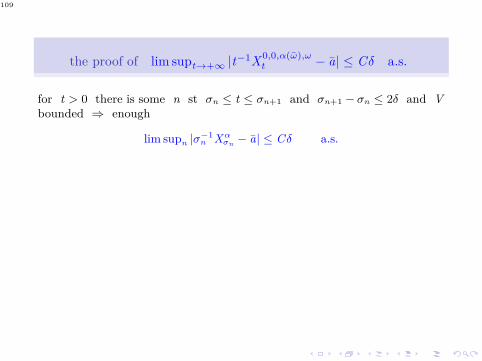
the proof of lim supt→+∞|t−1
X0,0,α(ω),ω
t − a| ≤ Cδ a.s.
for t > 0 there is some n st σn ≤ t ≤ σn+1 and σn+1 − σn ≤ 2δ and Vbounded ⇒ enough
lim supn |σ−1n Xα
σn− a| ≤ Cδ a.s.
110
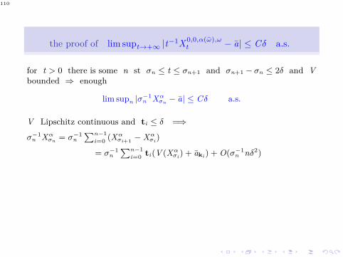
the proof of lim supt→+∞|t−1
X0,0,α(ω),ω
t − a| ≤ Cδ a.s.
for t > 0 there is some n st σn ≤ t ≤ σn+1 and σn+1 − σn ≤ 2δ and Vbounded ⇒ enough
lim supn |σ−1n Xα
σn− a| ≤ Cδ a.s.
V Lipschitz continuous and ti ≤ δ =⇒
σ−1n Xα
σn= σ−1
n
∑n−1
i=0(Xα
σi+1− Xα
σi)
= σ−1n
∑n−1
i=0ti(V (Xα
σi) + aki ) + O(σ−1
n nδ2)
111
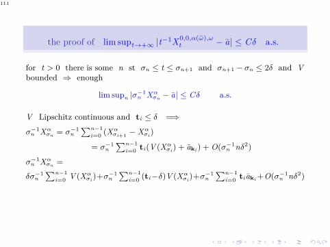
the proof of lim supt→+∞|t−1
X0,0,α(ω),ω
t − a| ≤ Cδ a.s.
for t > 0 there is some n st σn ≤ t ≤ σn+1 and σn+1 − σn ≤ 2δ and Vbounded ⇒ enough
lim supn |σ−1n Xα
σn− a| ≤ Cδ a.s.
V Lipschitz continuous and ti ≤ δ =⇒
σ−1n Xα
σn= σ−1
n
∑n−1
i=0(Xα
σi+1− Xα
σi)
= σ−1n
∑n−1
i=0ti(V (Xα
σi) + aki ) + O(σ−1
n nδ2)
σ−1n Xα
σn=
δσ−1n
∑n−1
i=0V (Xα
σi)+σ−1
n
∑n−1
i=0(ti −δ)V (Xα
σi)+σ−1
n
∑n−1
i=0ti aki +O(σ−1
n nδ2)
112
the proof of lim supt→+∞|t−1
X0,0,α(ω),ω
t − a| ≤ Cδ a.s.
for t > 0 there is some n st σn ≤ t ≤ σn+1 and σn+1 − σn ≤ 2δ and Vbounded ⇒ enough
lim supn |σ−1n Xα
σn− a| ≤ Cδ a.s.
V Lipschitz continuous and ti ≤ δ =⇒
σ−1n Xα
σn= σ−1
n
∑n−1
i=0(Xα
σi+1− Xα
σi)
= σ−1n
∑n−1
i=0ti(V (Xα
σi) + aki ) + O(σ−1
n nδ2)
σ−1n Xα
σn=
δσ−1n
∑n−1
i=0V (Xα
σi)+σ−1
n
∑n−1
i=0(ti −δ)V (Xα
σi)+σ−1
n
∑n−1
i=0ti aki +O(σ−1
n nδ2)
the law of large number =⇒
n−1σn → E(σ0) = δ; n−1∑n−1
i=0ti aki → δa;
n−1∑n−1
i=0|ti − δ| → E(|t0 − δ|) ≤ δ2


![1 Appendix: Common distributionsfaculty.chicagobooth.edu/nicholas.polson/teaching/41900/Appendices...1 Appendix: Common distributions ... Beta • A random variable X ∈ [0,1] has](https://static.fdocument.org/doc/165x107/5ae3e1407f8b9a595d8f03f5/1-appendix-common-appendix-common-distributions-beta-a-random-variable.jpg)