
RadialBasisFunctionRegularizationforLinearInverse ...my2550/papers/inverse.pdf ·...
29
Radial Basis Function Regularization for Linear Inverse Problems with Random Noise Carlos Valencia and Ming Yuan H. Milton Stewart School of Industrial and Systems Engineering Georgia Institute of Technology (February 20, 2011) Abstract In this paper, we study the statistical properties of method of regularization with radial basis functions in the context of linear inverse problems. Radial basis function regularization is widely used in machine learning because of its demonstrated effec- tiveness in numerous applications and computational advantages. From a statistical viewpoint, one of the main advantages of radial basis function regularization in gen- eral and Gaussian radial basis function regularization in particular is their ability to adapt to varying degree of smoothness in a direct problem. We show here that similar approaches for inverse problems not only share such adaptivity to the smoothness of the signal but also can accommodate different degrees of ill-posedness. These results render further theoretical support to the superior performance observed empirically for radial basis function regularization. Keywords: Inverse problem, minimax rate of convergence, radial basis function, regular- ization. 1
Transcript of RadialBasisFunctionRegularizationforLinearInverse ...my2550/papers/inverse.pdf ·...
Radial Basis Function Regularization for Linear Inverse
Problems with Random Noise
Carlos Valencia and Ming Yuan
H. Milton Stewart School of Industrial and Systems Engineering
Georgia Institute of Technology
(February 20, 2011)
Abstract
In this paper, we study the statistical properties of method of regularization with
radial basis functions in the context of linear inverse problems. Radial basis function
regularization is widely used in machine learning because of its demonstrated effec-
tiveness in numerous applications and computational advantages. From a statistical
viewpoint, one of the main advantages of radial basis function regularization in gen-
eral and Gaussian radial basis function regularization in particular is their ability to
adapt to varying degree of smoothness in a direct problem. We show here that similar
approaches for inverse problems not only share such adaptivity to the smoothness of
the signal but also can accommodate different degrees of ill-posedness. These results
render further theoretical support to the superior performance observed empirically for
radial basis function regularization.
Keywords: Inverse problem, minimax rate of convergence, radial basis function, regular-
ization.
1
1 Introduction
Radial basis function regularization is one of the most popular tools in machine learning (see,
e.g., Girosi, Jones, and Poggio (1993); Smola, Scholkopf, and Muller (1998); Wahba (1999);
Evgeniou, Pontil, and Poggio (2000); Lin and Brown (2004); Zhang, Genton and Liu (2004);
Lin and Yuan (2006); Shi and Yu (2006)). Let Φ(x) = φ(‖x‖) for vector x ∈ Rd be a radial
basis function where φ : [0,+∞) → R is a univariate function. Typical examples include
φ(r) = r2m log(r) (thin plate spline), φ(r) = e−r2/2 (Gaussian), and φ(r) = (c2 + r2)1/2
(multiquadrics) among others. When KΦ(x, y) = Φ(x−y) is (conditionally) positive definite
in that for any n ∈ Z and any distinct x1, ..., xn ∈ Rd,
n∑
j=1
n∑
k=1
ajakK(xj , xk) > 0,
Φ can be identified with a reproducing kernel Hilbert space (Aronszajn (1950)), denoted by
HΦ. The squared norm in HΦ can be written as
J(f) = (2π)−d/2
∫
Rd
|f(ω)|2/Φ(ω)dω
for any function f ∈ HΦ, where f stands for the Fourier transform of f , that is,
f(ω) = (2π)−d/2
∫
Rd
f(x)e−ixTωdx.
The method of regularization with a radial basis function estimates a functional parameter
by the solution to
minf∈HΦ
{L(f, data) + λJ(f)},
where L is the empirical loss, often taken to be the negative log-likelihood. The tuning
parameter λ > 0 controls the trade-off between minimizing the empirical loss and obtaining
a smooth solution.
Consider in particular estimating a periodic function f0 : [−π, π] → R based on noisy
observations of Af where A is a bounded linear operator, i.e.,
dY (t) = (Af0)(t)dt + ǫdW (t), t ∈ [−π, π]. (1)
Here ǫ > 0 is the noise level and W (t) is a standard Brownian motion on [−π, π]. The
white noise model (1) connects to a number of common statistical problems in the light
2
of results on its equivalence to nonparametric regression (Brown and Low, 1996), density
estimation (Nussbaum, 1996), spectral density estimation (Golubev and Nussbaum, 1998),
and nonparametric generalized regression (Grama and Nussbaum, 1997). The radial basis
function regularization in this case gives the following estimate of f0:
fλ = argminf∈HΦ
{
‖Y − Af‖2L2+ λJ(f)
}
.
Lin and Brown (2004) and Lin and Yuan (2006) recently studied the statistical properties
of fλ in a special case when A is the identity operator. They found that when f is a member of
any finite-order Sobolev spaces, the method of regularization with many radial basis functions
is rate optimal when the tuning parameter is appropriately chosen, which partially explains
the success of such methods in this particular setting. Of course in many applications, A is
not an identity operator but rather a general compact operator. Problems of this type can
be found in almost all areas of science and engineering (see, e.g., Chalmond (2008); Kaipo
and Somersalo (2004); Ramm (2009)). These problems, commonly referred to as inverse
problems, are often ill-posed and therefore, fundamentally more difficult than the case when
A is the identity, often referred to as direct problems (see, e.g., Cavalier (2008)). In this
paper, we study the statistical properties of radial basis function regularization estimator fλ
in this setting.
Similar to direct problems, the difficulty in estimating f0 in an inverse problem is de-
termined by the complexity of the functional class it belongs to. Differing from direct
problems, in an inverse problem, the difficulty of estimating f0 also depends on the degree
of ill-posedness of the linear operator A. We consider a variety of combinations of functional
classes and linear operators and show that for many common choices of radial basis functions,
fλ is rate optimal whenever λ is appropriately tuned. Our results suggest that the superior
statistical properties established earlier for the direct problems continue to hold in the in-
verse problems and therefore further make clear why the radial basis function regularization
is so effective in a wider range of applications.
The rest of this article is organized as follows. In the next section, we describe in more
details the parameter spaces and the ill-posedness of the problem. We study in Section 3
the statistical properties of radial basis function regularization. All proofs are relegated to
Section 6. Section 4 reports results from numerical experiments to illustrate the implications
of our theoretical development.
3
2 Radial Basis Function Regularization in Linear In-
verse Problems
The white noise model (1) can be expressed in terms of the corresponding Fourier coefficients
and leads to a sequence model that is often more amenable to statistical analysis (see, e.g.,
Johnstone, 1998).
2.1 Sequence model via singular value decomposition
Let A∗ be the adjoint operator of A. Because of the compactness of A, A∗A admits spectral
decomposition
A∗Af =∞∑
k=1
b2k〈f, ϕk〉L2ϕk (2)
for any square integrable periodic function f , where the eigenfunctions {ϕ1, ϕ2, . . .} consti-
tute an orthornormal basis of L2, the collection of square integrable periodic functions, and
the eigenvalues {b21, b22, . . .} are arranged in a non-increasing order without loss of generality.
Denote by ψk the normalized image of ϕk, that is, Aϕk = bkψk. It is easy to show that
A∗ψk = bkϕk.
From the singular value decomposition, we can convert the linear inverse problem (1) into a
sequence model. More specifically,
yk := 〈Y, ψk〉L2 = 〈Af0, ψk〉L2 + 〈ǫW, ψk〉L2 = bk〈f0, ϕk〉L2 + ǫ〈W,ψk〉L2 =: bkθk + ǫξk
for k = 1, 2, . . ..
Unlike the direct problem where all singular values are one, in an inverse problem, bk → 0
as k → ∞. The vanishing singular values poses challenges in inverting the linear operator A
and makes the problem ill-posed. As a result, the estimation of f0 becomes fundamentally
more difficult for an inverse problem than for a direct problem. The rate of decay of {bk :
k ≥ 1} quantifies the ill-posedness. Typically, an inverse problem is called mildly ill-posed
if bk ∼ k−β and severe ill-posed if bk ∼ exp(−βk) for some parameter β > 0 often referred
to as the degree of ill-posedness. Hereafter, ak ∼ bk means that both ak/bk and bk/ak are
bounded away from zero.
4
2.2 Parameter spaces
In addition to the ill-posedness, the difficulty of estimating f0 in (1) is also determined
by the parameter space for the functional parameter. It is often convenient to describe
the parameters space using the Fourier coefficient with respect to the basis {ϕk : k ≥ 1}.
Typically, f0 belongs to the functional class corresponding to an ellipsoid Θ in the space of
Fourier coefficients {θk : k ≥ 1}:
Θ =
{
(θk : k ≥ 1) :∑
k≥1
a2kθ2k ≤ Q
}
, (3)
for a non-deceasing sequence 0 ≤ a1 ≤ a2 ≤ . . . such that ak → ∞ as k → ∞, and a positive
constant Q.
It is instructive to consider the case when {ϕk : k ≥ 1} is the usual trigonometric basis,
that is, ϕ1(t) = (2π)−1/2, ϕ2l(t) = π−1/2 sin(lt) and ϕ2l+1(t) = π−1/2 cos(lt) for l ≥ 1. In this
case, the usual Sobolev spaces are perhaps the most popular examples of Θ. Let Sm(Q) be
the mth order Sobolev space of periodic functions on [−π, π], that is,
Sm(Q) =
{
f ∈ L2 : f is 2π−periodic, and
∫ π
−π
f 2 + (f (m))2 ≤ Q
}
.
Simple calculation shows that Sm(Q) can also be equivalently expressed as
Sm(Q) =
{
f ∈ L2 : f =∑
k≥1
θkϕk,∑
k≥1
a2kθ2k ≤ Q, a1 = 1, a2l = a2l+1 = k2m + 1
}
.
In the same spirit, analytic functions or sometimes referred to as infinit-order Sobolev space
can be described as
S∞(α;Q) =
{
f ∈ L2 : f =∑
k≥1
θkϕk,∑
k≥1
a2kθ2k ≤ Q, a1 = 1, a2l = a2l+1 = eαl
}
.
See Johnstone (1998) for details.
Appealing to this connection, in what follows, we shall write
Θα(Q) =
{
(θk : k ≥ 1) :∑
k≥1
a2kθ2k ≤ Q, a1 = 1, a2l = a2l+1 = kα + 1
}
as Sobolev type of spaces of order α; and
Θ∞(α;Q) =
{
(θk : k ≥ 1) :∑
k≥1
a2kθ2k ≤ Q, a1 = 1, a2l = a2l+1 = eαk
}
to represent spaces similar to S∞.
5
2.3 Radial basis function regularization
We now describe the radial basis functions and the reproducing kernel Hilbert spaces they
induce. Because we focus here on periodic functions, it is natural to consider periodized
radial basis functions
Φ0(r) =∑
k∈Z
Φ(r − 2πk),
where Φ is a radial basis function. See Smola, Scholkopf and Muller (1998), Lin and Brown
(2004) among others for further discussion of periodized radial basis functions and their
applications in machine learning. As shown in Lin and Yuan (2006), Φ0 (or equivalently
KΦ0) is positive definite so long as Φ is positive definite and furthermore the norm of HΦ0
can be given by
‖f‖2HΦ0=∑
k≥1
γkθ2k,
where θks are the Fourier coefficients of f , and γ1 = (2π)−1/2{Φ(0)}−1, γ2l = γ2l+1 =
(2π)−1/2{Φ(l)}−1, l = 1, 2, . . .. When {ϕk : k ≥ 1} is taken to be the classical trigono-
metric basis, the method of regularization with radial basis function Φ0 can be equivalently
expressed in terms of the sequence of Fourier coefficients:
fλ = argminf=
∑k≥0 θkϕk∈HΦ0
{
∑
k≥1
(yk − bkθk)2 + λ
∑
k≥1
γkθ2k
}
.
Consider, for example, the periodic Gaussian kernel
G0(r) =∑
k∈Z
G(r − 2πk),
where
G(r) =1
√
2π2exp
(
−r2
22
)
for some parameter > 0. Simple calculation yields that γ2l = γ2l+1 = el22/2. Other
popular examples include periodic multiquadratics and Wendland kernels (Wendland (1998))
that corresponds to γ2l = γ2l+1 = el and γ2l = γ2l+1 = k respectively. There are also
other common choices of radial basis functions for which γk behaves similarly to these three
examples. See Buhlmann (2003) for further details.
6
3 Main Results
Following the discussion before, we shall focus on the following sequence model hereafter:
yk = bkθk + ǫξk, k = 1, 2, . . . . (4)
The inverse problem under investigation is either mildly or severely ill-posed, that is, bk ∼
k−β or bk ∼ e−βk respectively. We shall also consider Sobolev type of parameter spaces, that
is, (θk : k ≥ 1) ∈ Θα for some α > 1/2 or Θ∞(α,Q). Our primary interest is to evaluate the
statistical performance of radial basis function regularization:
(θkλ : k ≥ 1) = argmin(ηk :k≥1)
{
∑
k≥1
(yk − bkηk)2 + λ
∑
k≥1
γkη2k
}
. (5)
In particular, we consider three different types of radial basis functions: (1) γk ∼ eγk2for
some γ > 0 with periodic Gaussian kernel as a typical example; (2) γk ∼ eγk with periodic
multiquadrics kernel as a typical example; and (3) γk ∼ kγ with periodic Wendland kernel
or the usual spline kernels (see, e.g., Wahba (1990)) as typical examples.
We begin with Gaussian type of kernel, that is, γk ∼ eγk2for some γ > 0.
Theorem 1 Assume that γk ∼ eγk2for some γ > 0.
(a) (Mildly ill-posed with Sobolev spaces) If bk ∼ k−β and
λ ∼ exp(
−ǫ4
2α+2β+1
)
,
then
sup(θk:k≥1)∈Θα(Q)
∑
k≥1
E
(
θkλ − θk
)2
∼ ǫ4α
2α+2β+1 .
(b) (Mildly ill-posed with analytic functions) If bk ∼ k−β and
λ ∼ exp
(
−γ
4α2
(
log1
ǫ2
)2)
,
then
sup(θk :k≥1)∈Θ∞(α,Q)
∑
k≥1
E
(
θkλ − θk
)2
∼ ǫ2(
log1
ǫ2
)2β+1
.
7
(c) (Severely ill-posed with Sobolev spaces) If bk ∼ k−β and
λ ∼ exp
(
−
(
log1
ǫ2
)2)
,
then
sup(θk :k≥1)∈Θα(Q)
∑
k≥1
E
(
θkλ − θk
)2
∼
(
log1
ǫ
)−2α
.
(d) (Severely ill-posed with analytic functions) If bk ∼ e−βk and
λ ∼ exp
(
−γ
(2α + 2β)2
(
log1
ǫ2
)2)
,
then
sup(θk:k≥1)∈Θ∞(α,Q)
∑
k≥1
E
(
θkλ − θk
)2
∼ ǫ2α
α+β .
We note that all the rates obtained in Theorem 1 are minimax optimal (see, e.g., Cavalier
(2008)). In other words, when the tuning parameter λ is appropriately chosen, Gaussian
radial basis function regularization is rate optimal for all combinations of ill-posedness as
well as parameter spaces. This result, together with similar results for direct problems (Lin
and Brown (2004)), partly explain its success in numerous applications.
Next we consider the case with a multiquadrics type of kernel.
Theorem 2 Assume that γk ∼ eγk for some γ > 0.
(a) (Mildly ill-posed with Sobolev spaces) If bk ∼ k−β and
λ ∼ exp(
−ǫ−2
2α+2β+1
)
,
then
sup(θk:k≥1)∈Θα(Q)
∑
k≥1
E
(
θkλ − θk
)2
∼ ǫ4α
2α+2β+1 .
(b) (Mildly ill-posed with analytic functions) If bk ∼ k−β, then
sup(θk :k≥1)∈Θ∞(α,Q)
∑
k≥1
E
(
θkλ − θk
)2
∼ ǫ2(
log1
ǫ2
)2β+1
.
provided that
λ ∼
ǫγα γ > α− 2β
ǫ γ ≤ α− 2β.
8
(c) (Severely ill-posed with Sobolev spaces) If bk ∼ k−β and λ ∼ ǫ2, then
sup(θk :k≥1)∈Θα(Q)
∑
k≥1
E
(
θkλ − θk
)2
∼
(
log1
ǫ
)−2α
.
(d) (Severely ill-posed with analytic functions) Suppose that bk ∼ e−βk. If γ > α− 2β and
λ ∼ ǫ−β+γα+β ,
then
sup(θk:k≥1)∈Θ∞(α,Q)
∑
k≥1
E
(
θkλ − θk
)2
∼ ǫ2α
α+β .
If γ ≤ α− 2β, then the best achievable rate is
sup(θk:k≥1)∈Θ∞(α,Q)
∑
k≥1
E
(
θkλ − θk
)2
∼ ǫ4β+2γ3β+γ ,
and it is attained when
λ ∼ ǫ2β+γ3β+γ .
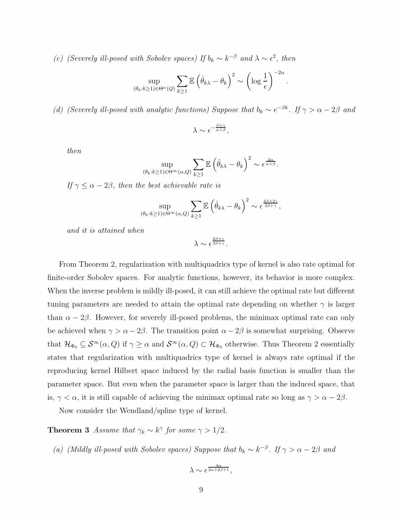
From Theorem 2, regularization with multiquadrics type of kernel is also rate optimal for
finite-order Sobolev spaces. For analytic functions, however, its behavior is more complex.
When the inverse problem is mildly ill-posed, it can still achieve the optimal rate but different
tuning parameters are needed to attain the optimal rate depending on whether γ is larger
than α − 2β. However, for severely ill-posed problems, the minimax optimal rate can only
be achieved when γ > α− 2β. The transition point α− 2β is somewhat surprising. Observe
that HΦ0 ⊆ S∞(α,Q) if γ ≥ α and S∞(α,Q) ⊂ HΦ0 otherwise. Thus Theorem 2 essentially
states that regularization with multiquadrics type of kernel is always rate optimal if the
reproducing kernel Hilbert space induced by the radial basis function is smaller than the
parameter space. But even when the parameter space is larger than the induced space, that
is, γ < α, it is still capable of achieving the minimax optimal rate so long as γ > α− 2β.
Now consider the Wendland/spline type of kernel.
Theorem 3 Assume that γk ∼ kγ for some γ > 1/2.
(a) (Mildly ill-posed with Sobolev spaces) Suppose that bk ∼ k−β. If γ > α− 2β and
λ ∼ ǫ4α
2α+2β+1 ,
9

then
sup(θk:k≥1)∈Θα(Q)
∑
k≥1
E
(
θkλ − θk
)2
∼ ǫ4α
2α+2β+1 .
If γ ≤ α− 2β, the best achivable rate is
sup(θk :k≥1)∈Θα(Q)
∑
k≥1
E
(
θkλ − θk
)2
∼ ǫ2(4β+2γ)6β+2γ+1 ,
and it is attained when
λ ∼ ǫ4β+2γ
6β+2γ+1 .
(b) (Mildly ill-posed with analytic functions) Suppose the bk ∼ k−β. If γ > α− 2β and
λ ∼ ǫ2(
log1
ǫ
)−2β−γ
,
then
sup(θk :k≥1)∈Θα(Q)
∑
k≥1
E
(
θkλ − θk
)2
∼ ǫ2(
log1
ǫ
)2β+1
.
If γ ≤ α− 2β, the best achievable rate is
sup(θk :k≥1)∈Θα(Q)
∑
k≥1
E
(
θkλ − θk
)2
∼ ǫ2(4β+2γ)6β+2γ+1 ,
and it is attained when
λ ∼ ǫ4β+2γ
6β+2γ+1 .
(c) (Severely ill-posed with Sobolev spaces) If bk ∼ e−βk
λ ∼ ǫ2
then
sup(θk :k≥1)∈Θα(Q)
∑
k≥1
E
(
θkλ − θk
)2
∼
(
log1
ǫ
)−2α
(d) (Severely ill-posed with analytic functions) Suppose bk ∼ e−βk. If γ > α− 2β, then the
achievable rate is
sup(θk:k≥1)∈Θα(Q)
∑
k≥1
E
(
θkλ − θk
)2
∼ ǫ2β
α+2β ,
and it is attained when
λ ∼ ǫ4β
α+2β .
10
When γ ≤ α− 2β, the best achievable rate is
sup(θk:k≥1)∈Θα(Q)
∑
k≥1
E
(
θkλ − θk
)2
∼ ǫ43 ,
and it is attained when λ ∼ ǫ23 .
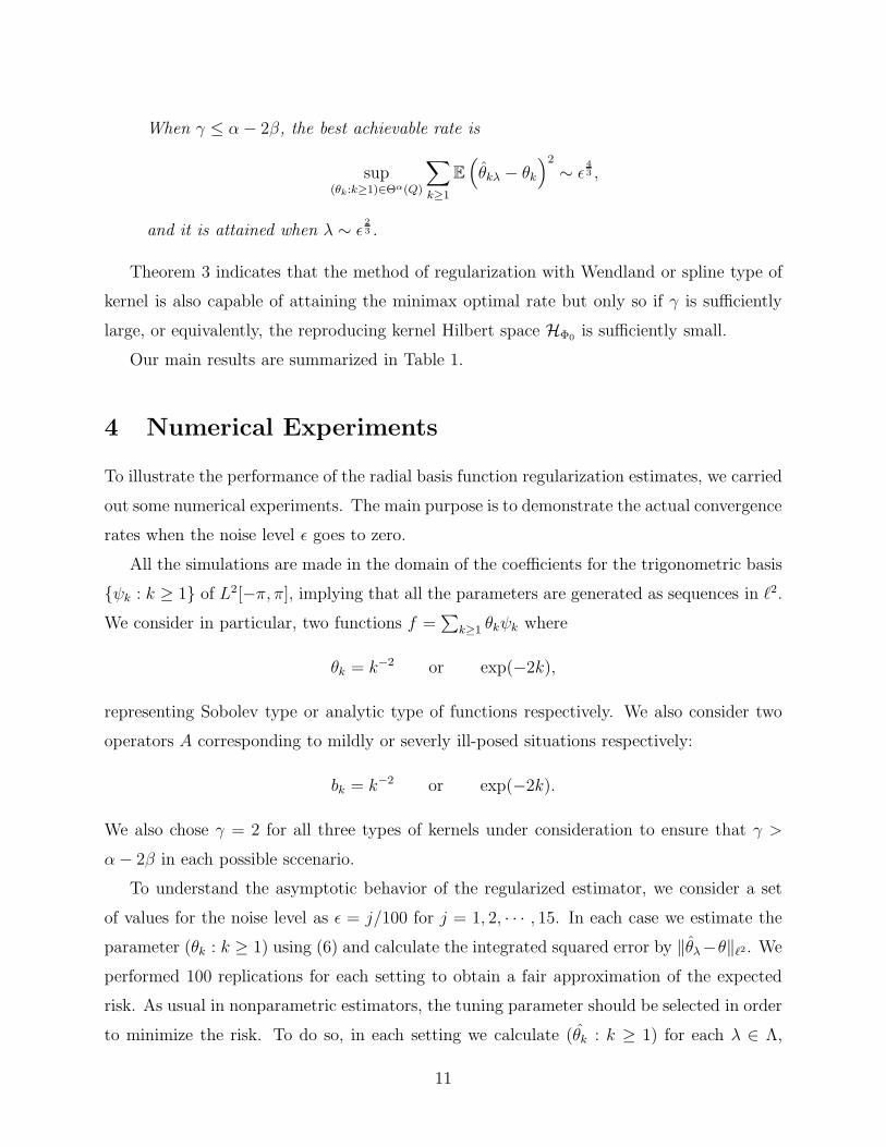
Theorem 3 indicates that the method of regularization with Wendland or spline type of
kernel is also capable of attaining the minimax optimal rate but only so if γ is sufficiently
large, or equivalently, the reproducing kernel Hilbert space HΦ0 is sufficiently small.
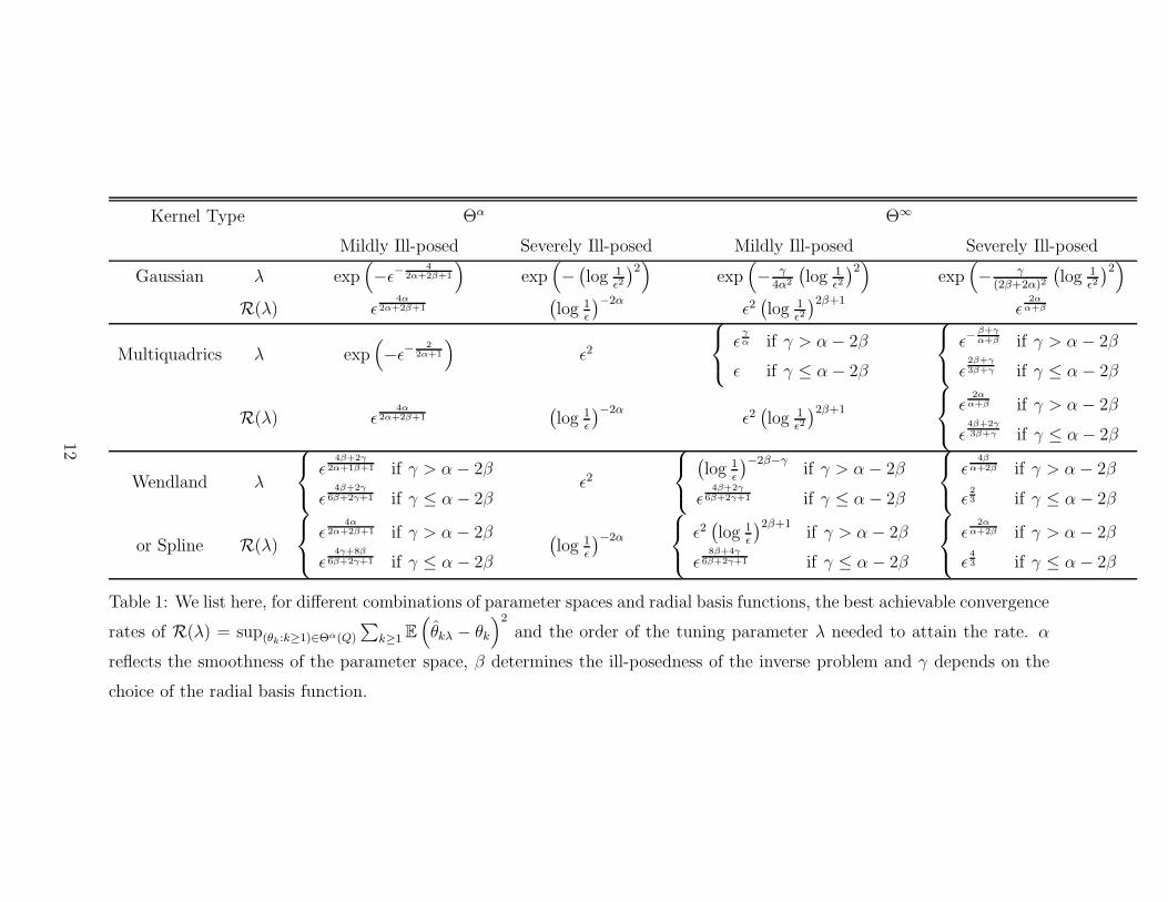
Our main results are summarized in Table 1.
4 Numerical Experiments
To illustrate the performance of the radial basis function regularization estimates, we carried
out some numerical experiments. The main purpose is to demonstrate the actual convergence
rates when the noise level ǫ goes to zero.
All the simulations are made in the domain of the coefficients for the trigonometric basis
{ψk : k ≥ 1} of L2[−π, π], implying that all the parameters are generated as sequences in ℓ2.
We consider in particular, two functions f =∑
k≥1 θkψk where
θk = k−2 or exp(−2k),
representing Sobolev type or analytic type of functions respectively. We also consider two
operators A corresponding to mildly or severly ill-posed situations respectively:
bk = k−2 or exp(−2k).
We also chose γ = 2 for all three types of kernels under consideration to ensure that γ >
α− 2β in each possible sccenario.
To understand the asymptotic behavior of the regularized estimator, we consider a set
of values for the noise level as ǫ = j/100 for j = 1, 2, · · · , 15. In each case we estimate the
parameter (θk : k ≥ 1) using (6) and calculate the integrated squared error by ‖θλ−θ‖ℓ2 . We
performed 100 replications for each setting to obtain a fair approximation of the expected
risk. As usual in nonparametric estimators, the tuning parameter should be selected in order
to minimize the risk. To do so, in each setting we calculate (θk : k ≥ 1) for each λ ∈ Λ,
11
Kernel Type Θα Θ∞
Mildly Ill-posed Severely Ill-posed Mildly Ill-posed Severely Ill-posed
Gaussian λ exp(
−ǫ−4
2α+2β+1
)
exp(
−(
log 1ǫ2
)2)
exp(
− γ4α2
(
log 1ǫ2
)2)
exp(
− γ(2β+2α)2
(
log 1ǫ2
)2)
R(λ) ǫ4α
2α+2β+1(
log 1ǫ
)−2αǫ2(
log 1ǫ2
)2β+1ǫ
2αα+β
Multiquadrics λ exp(
−ǫ−2
2α+1
)
ǫ2
ǫγα if γ > α− 2β
ǫ if γ ≤ α− 2β
ǫ−β+γα+β if γ > α− 2β
ǫ2β+γ3β+γ if γ ≤ α− 2β
R(λ) ǫ4α
2α+2β+1(
log 1ǫ
)−2αǫ2(
log 1ǫ2
)2β+1
ǫ2α
α+β if γ > α− 2β
ǫ4β+2γ3β+γ if γ ≤ α− 2β
Wendland λ
ǫ4β+2γ
2α+1β+1 if γ > α− 2β
ǫ4β+2γ
6β+2γ+1 if γ ≤ α− 2βǫ2
(
log 1ǫ
)−2β−γif γ > α− 2β
ǫ4β+2γ
6β+2γ+1 if γ ≤ α− 2β
ǫ4β
α+2β if γ > α− 2β
ǫ23 if γ ≤ α− 2β
or Spline R(λ)
ǫ4α
2α+2β+1 if γ > α− 2β
ǫ4γ+8β
6β+2γ+1 if γ ≤ α− 2β
(
log 1ǫ
)−2α
ǫ2(
log 1ǫ
)2β+1if γ > α− 2β
ǫ8β+4γ
6β+2γ+1 if γ ≤ α− 2β
ǫ2α
α+2β if γ > α− 2β
ǫ43 if γ ≤ α− 2β
Table 1: We list here, for different combinations of parameter spaces and radial basis functions, the best achievable convergence
rates of R(λ) = sup(θk:k≥1)∈Θα(Q)
∑
k≥1E
(
θkλ − θk
)2
and the order of the tuning parameter λ needed to attain the rate. α
reflects the smoothness of the parameter space, β determines the ill-posedness of the inverse problem and γ depends on the
choice of the radial basis function.
12
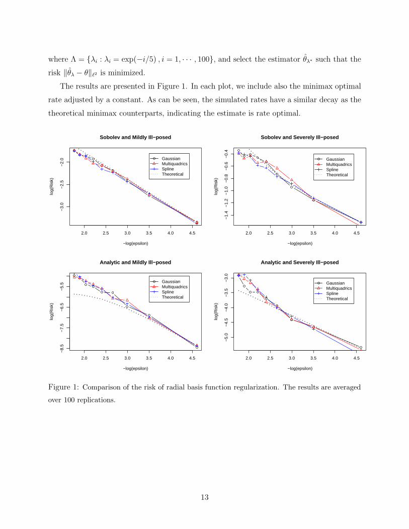
where Λ = {λi : λi = exp(−i/5) , i = 1, · · · , 100}, and select the estimator θλ∗ such that the
risk ‖θλ − θ‖ℓ2 is minimized.
The results are presented in Figure 1. In each plot, we include also the minimax optimal
rate adjusted by a constant. As can be seen, the simulated rates have a similar decay as the
theoretical minimax counterparts, indicating the estimate is rate optimal.
2.0 2.5 3.0 3.5 4.0 4.5
−3.
0−
2.5
−2.
0
Sobolev and Mildly Ill−posed
−log(epsilon)
log(
Ris
k)
GaussianMultiquadricsSplineTheoretical
2.0 2.5 3.0 3.5 4.0 4.5
−1.
4−
1.2
−1.
0−
0.8
−0.
6−
0.4
Sobolev and Severely Ill−posed
−log(epsilon)
log(
Ris
k)
GaussianMultiquadricsSplineTheoretical
2.0 2.5 3.0 3.5 4.0 4.5
−8.
5−
7.5
−6.
5−
5.5
Analytic and Mildly Ill−posed
−log(epsilon)
log(
Ris
k)
GaussianMultiquadricsSplineTheoretical
2.0 2.5 3.0 3.5 4.0 4.5
−5.
0−
4.5
−4.
0−
3.5
−3.
0
Analytic and Severely Ill−posed
−log(epsilon)
log(
Ris
k)
GaussianMultiquadricsSplineTheoretical
Figure 1: Comparison of the risk of radial basis function regularization. The results are averaged
over 100 replications.
13

5 Risk Analysis of Radial Basis Function Regulariza-
tion
We now set out to establish the results presented in the previous section. Recall that the
regularization estimator (θkλ : k ≥ 1) is defined as
(θkλ : k ≥ 1) = argmin(ηk :k≥1)
{
∑
k≥1
(yk − bkηk)2 + λ
∑
k≥1
γkη2k
}
.
It can be written explicitly as
θkλ =bk
b2k + λγ−1k
yk , k = 1, 2, · · · . (6)
In particular, here we consider
bk ∼
k−β Mildly ill− posed
exp(−βk) Severely ill− posed.
Furthermore, the true Fourier coefficients (θk : k ≥ 1) are assumed to be in an ellipsiod
Θ(Q) =
{
(θk : k ≥ 1) :∑
k≥1
a2kθ2k ≤ Q
}
,
where
ak ∼
kα Θ = Θα(Q)
exp(αk) Θ = Θ∞(α;Q).
Observe that the risk of the radial basis function regularization estimator (θkλ : k ≥ 1) can
be decomposed as the sum of the squared bias and the variance:
∑
k≥1
E
(
θkλ − θk
)2
=∑
k≥1
(
Eθkλ − θk
)2
+∑
k≥1
Var(
θkλ
)
=: B2θ
(
θλ
)
+Varθ
(
θλ
)
. (7)
By (6), we can further write
B2θ
(
θλ
)
=∑
k≥1
λ2γ−2k θ2k
(
b2k + λγ−1k
)2
and
Varθ
(
θλ
)
= ǫ2∑
k≥1
b2k(
b2k + λγ−1k
)2 .
14

The squared bias and variance can be further bounded as follows:
B2θ
(
θλ
)
≤ maxk
{
λ2γ−2k a−2
k(
b2k + λγ−1k
)2
}(
∑
k≥1
a2kθ2k
)
≤ maxk
(
λ2γ−2k a−2
k
b4k + λ2γ−2k
)
(
∑
k≥1
a2kθ2k
)
, (8)
and
Varθ
(
θλ
)
≤ ǫ2∑
k≥1
b2kγ2k
b4kγ2k + λ2
. (9)
5.1 Proof of Theorem 1
We begin with the case when γk ∼ eγk2for some γ > 0.
5.1.1 Mildly ill-posed with Sobolev spaces
In this case, bk ∼ k−β and ak ∼ kα. From (8)
supθ∈Θα(Q)
B2θ
(
θλ
)
≤ Cλ2(
minx≥1
{
x2α−4β exp(−2γx2) + λ2x2α}
)−1
. (10)
Hereafter we use C as a generic positive constant which may take different values at each
appearance. By the first order condition, the minimum on the right hand side is achieved
at the root of(
2α− 4β
x− 4γx
)
x2α−4β exp(−2γx2) +2αλ2
xx2α = 0,
implying that
supθ∈Θα(Q)
B2θ
(
θλ
)
≤ C (− log λ)−α . (11)
Now consider Varθ
(
θλ
)
. From (9)
Varθ
(
θλ
)
≤ ǫ2∑
k≥1
k−2β exp(−2γk2)
k−4β exp(−2γk2) + λ2≈ ǫ2
∫ ∞
1
x−2β exp(−2γx2)
x−4β exp(−2γx2) + λ2dx.
The integral on the rightmost hand side can be bounded by
∫ ∞
1
1
x−2β + λ2x2β exp(2γx2)dx ≤
∫ x0
1
x2βdx+
∫ ∞
x0
λ−2x−2β exp(−2γx2)dx,
where x0 is the positive root of
x−2β = λ2x2β exp(2γx2),
15

which is of the order (−γ−1 log λ)12 . Because
∫ ∞
x0
λ−2x−2β exp(−2γx2)dx = o(
x2β0
)
,
for small values of λ, we have
∑
k≥1
Var(
θkλ
)
= O
(
ǫ2(
log1
λ
)2α+ 12
)
(12)
as λ→ 0.
Combining (11) and (12), we have
∑
k≥1
E
(
θkλ − θk
)2
= O
(
(
log1
λ
)−α
+ ǫ2(
log1
λ
)β+1/2)
as ǫ→ 0. Taking
λ = O(
exp(
−ǫ4
2α+2β+1
))
yields
sup(θk:k≥1)∈Θα(Q)
∑
k≥1
E
(
θkλ − θk
)2
= O(
exp(
−ǫ4α
2α+2β+1
))
,
as ǫ→ 0.
5.1.2 Mildly ill-posed with analytic function
For this case, bk ∼ k−β and ak ∼ exp(αk). First observe that the variance Varθ
(
θλ
)
does
not change with the parameter space and can still be bounded as in (12). On the other
hand, from (8),
sup(θk:k≥1)∈Θ∞(α,Q)
B2θ
(
θλ
)
≤ Cλ2(
minx≥1
{
x−4β exp(2αx− 2γx2) + λ2 exp(2αx)}
)−1
,
and following the first order condition for the minimization on the right hand side, we have
sup(θk:k≥1)∈Θ∞(α,Q)
B2θ
(
θλ
)
= O
(
exp
[
−2α
(
−1
γlog λ
)1/2])
, (13)
as λ→ 0. Summing up, we have
∑
k≥1
E
(
θkλ − θk
)2
= O
(
exp
[
−2α
(
−1
γlog λ
)1/2]
+ ǫ2(
log1
λ
)β+1/2)
, (14)
16
as ǫ→ 0. Consequently, if λ takes the optimal value
λ = O
(
exp
(
−γ
2α2
(
log1
ǫ2
)2))
,
the risk is minimax rate optimal, i.e.,
sup(θk :k≥1)∈Θ∞(α,Q)
∑
k≥1
E
(
θkλ − θk
)2
= O
(
ǫ2(
log1
ǫ
)2β+1)
,
as ǫ→ 0.
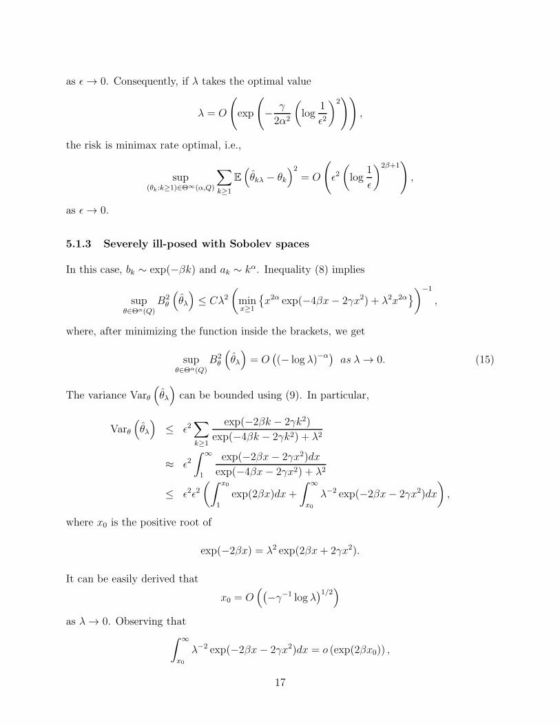
5.1.3 Severely ill-posed with Sobolev spaces
In this case, bk ∼ exp(−βk) and ak ∼ kα. Inequality (8) implies
supθ∈Θα(Q)
B2θ
(
θλ
)
≤ Cλ2(
minx≥1
{
x2α exp(−4βx− 2γx2) + λ2x2α}
)−1
,
where, after minimizing the function inside the brackets, we get
supθ∈Θα(Q)
B2θ
(
θλ
)
= O(
(− log λ)−α) as λ→ 0. (15)
The variance Varθ
(
θλ
)
can be bounded using (9). In particular,
Varθ
(
θλ
)
≤ ǫ2∑
k≥1
exp(−2βk − 2γk2)
exp(−4βk − 2γk2) + λ2
≈ ǫ2∫ ∞
1
exp(−2βx− 2γx2)dx
exp(−4βx− 2γx2) + λ2
≤ ǫ2ǫ2(∫ x0
1
exp(2βx)dx+
∫ ∞
x0
λ−2 exp(−2βx− 2γx2)dx
)
,
where x0 is the positive root of
exp(−2βx) = λ2 exp(2βx+ 2γx2).
It can be easily derived that
x0 = O(
(
−γ−1 log λ)1/2)
as λ→ 0. Observing that∫ ∞
x0
λ−2 exp(−2βx− 2γx2)dx = o (exp(2βx0)) ,
17
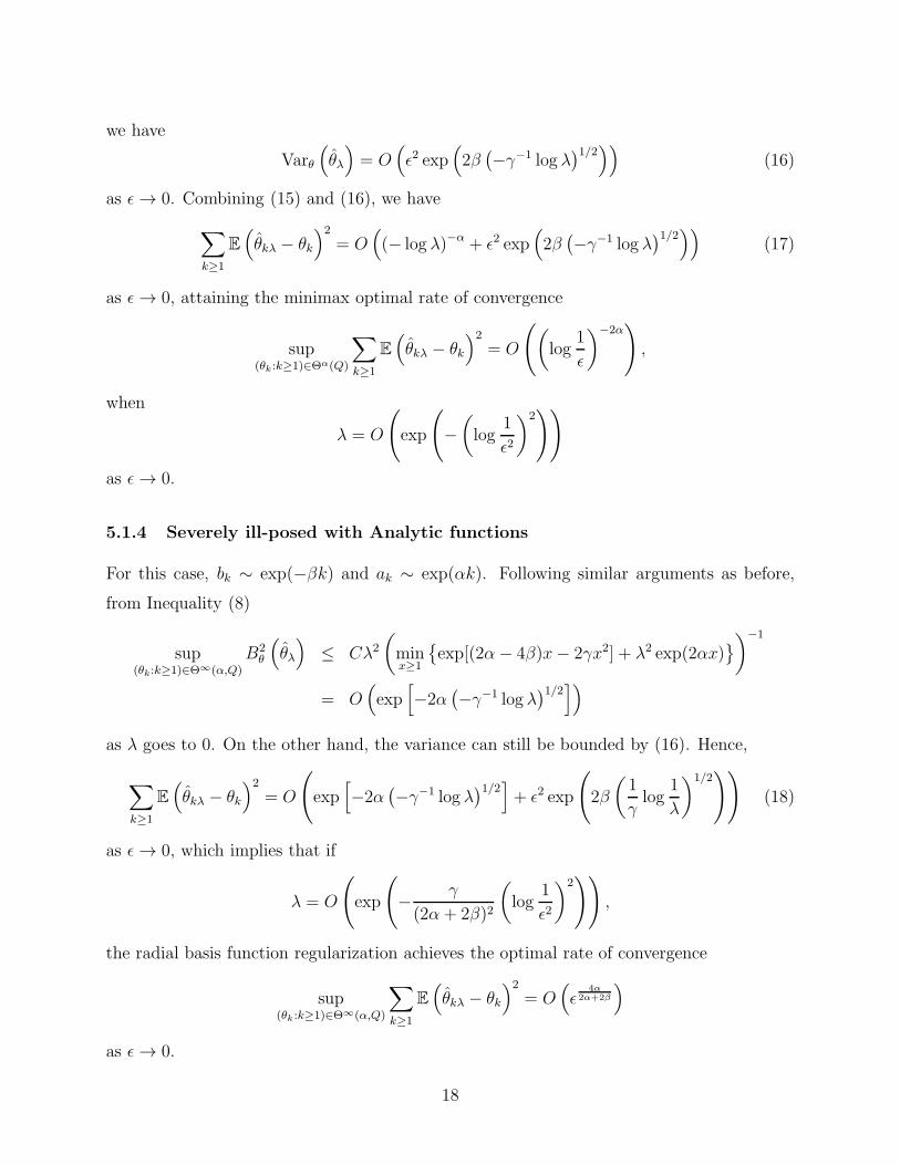
we have
Varθ
(
θλ
)
= O(
ǫ2 exp(
2β(
−γ−1 log λ)1/2))
(16)
as ǫ→ 0. Combining (15) and (16), we have
∑
k≥1
E
(
θkλ − θk
)2
= O(
(− log λ)−α + ǫ2 exp(
2β(
−γ−1 log λ)1/2))
(17)
as ǫ→ 0, attaining the minimax optimal rate of convergence
sup(θk :k≥1)∈Θα(Q)
∑
k≥1
E
(
θkλ − θk
)2
= O
(
(
log1
ǫ
)−2α)
,
when
λ = O
(
exp
(
−
(
log1
ǫ2
)2))
as ǫ→ 0.
5.1.4 Severely ill-posed with Analytic functions
For this case, bk ∼ exp(−βk) and ak ∼ exp(αk). Following similar arguments as before,
from Inequality (8)
sup(θk:k≥1)∈Θ∞(α,Q)
B2θ
(
θλ
)
≤ Cλ2(
minx≥1
{
exp[(2α− 4β)x− 2γx2] + λ2 exp(2αx)}
)−1
= O(
exp[
−2α(
−γ−1 log λ)1/2])
as λ goes to 0. On the other hand, the variance can still be bounded by (16). Hence,
∑
k≥1
E
(
θkλ − θk
)2
= O
(
exp[
−2α(
−γ−1 log λ)1/2]
+ ǫ2 exp
(
2β
(
1
γlog
1
λ
)1/2))
(18)
as ǫ→ 0, which implies that if
λ = O
(
exp
(
−γ
(2α + 2β)2
(
log1
ǫ2
)2))
,
the radial basis function regularization achieves the optimal rate of convergence
sup(θk :k≥1)∈Θ∞(α,Q)
∑
k≥1
E
(
θkλ − θk
)2
= O(
ǫ4α
2α+2β
)
as ǫ→ 0.
18

5.2 Proof of Theorem 2
We now consider the case when γk ∼ eγk.
5.2.1 Mildly ill-posed with Sobolev spaces
Observe that bk ∼ k−β and ak ∼ kα. From (8),
supθ∈Θα(Q)
B2θ
(
θλ
)
≤ Cλ2(
minx≥1
{xα−2β exp(−γx) + λxα}
)−2
.
By the first order condition, the minimun is acieved when x is the root of the equation
(
x−1(α− 2β)− γ)
xα−2β exp(−γx) + αλxα−1 = 0,
whose solution, after simple algebraic manipulations, implies
supθ∈Θα(Q)
B2θ
(
θλ
)
= O(
(− log λ)−2α) (19)
as λ becomes small. On the other hand, in the light of (9),
Varθ
(
θλ
)
≤ ǫ2∞∑
k=1
k−2β exp(−2γk)
k−4β exp(−2γk) + λ2≈ ǫ2
∫ ∞
1
dx
x−2β + λ2x2β exp(2γx),
where the integral on the right hand side can be bounded by
∫ x0
1
x2βdx+
∫ ∞
x0
λ−2x−2β exp(−2γx)dx,
and x0 is the positive root of
x−2β = λ2x2β exp(2γx).
It is easy to check that
x0 = O(
−γ−1 log λ)
as λ→ 0. Observing that
∫ ∞
x0
λ−2x−2β exp(−2γx)dx = o(
x2β0
)
,
we have
Varθ
(
θλ
)
= O(
ǫ2 (− log λ)2β+1)
(20)
19

as ǫ→ 0. Combining (19) and (20), we have
∑
k≥1
E
(
θkλ − θk
)2
= O(
(− log λ)−2α + ǫ2 (− log λ)2β+1)
, (21)
which implies that if
λ = O(
exp(
−ǫ−2
2α+2β+1
))
,
it achieves the minimax optimal rate of convergence
sup(θk:k≥1)∈Θα(Q)
∑
k≥1
E
(
θkλ − θk
)2
= O(
ǫ4α
2α+2β+1
)
as ǫ→ 0.
5.2.2 Mildly ill-posed with analytic function
In this case, bk ∼ k−β and ak ∼ exp(αk). From (8),
sup(θk:k≥1)∈Θ∞(α,Q)
B2θ
(
θλ
)
≤ Cλ2(
minx≥1
{x−4β exp(2αx− 2γx) + λ2 exp(2αx)}
)−1
.
By the first order condition, the minimum on the right hand side is attained at the root of
(
−4βx−1 + 2α− 2γ)
x−4β exp(−2γx) + 2αλ2 = 0.
Thus,
sup(θk:k≥1)∈Θ∞(α,Q)
B2θ
(
θλ
)
=
O(
exp(
2αγlog(λ)
))
if γ > α− 2β
O (λ2) if γ ≤ α− 2β. (22)
Combining (22) and the bound on the variance given in (20), we have
(a) if γ > α− 2β,
sup(θk:k≥1)∈Θ∞(α,Q)
∑
k≥1
E
(
θkλ − θk
)2
= O
(
exp
(
2α
γlog(λ)
)
+ ǫ2 (− log λ)2β+1
)
;
(b) if γ ≤ α− 2β.
sup(θk:k≥1)∈Θ∞(α,Q)
∑
k≥1
E
(
θkλ − θk
)2
= O(
λ2 + ǫ2 (− log λ)2β+1)
.
20

Taking
λ =
O(
ǫγα
)
if γ > α− 2β
O(ǫ) if γ ≤ α− 2β,
the radial basis function regularization achieves the minimax optimal rate of
sup(θk :k≥1)∈Θ∞(α,Q)
∑
k≥1
E
(
θkλ − θk
)2
= O
(
ǫ2(
log1
ǫ
)2β+1)
,
as ǫ→ 0.
5.2.3 Severely ill-posed with Sobolev spaces
Observe that bk ∼ exp(−βk) and ak ∼ kα. From (8),
sup(θk :k≥1)∈Θα(Q)
B2θ
(
θλ
)
≤ Cλ2(
minx≥1
{xα exp(−2βx− γx) + λxα}
)−2
= O(
(− log λ)−2α)
as λ goes to 0. To bound the variance, note that from (9),
∑
k≥1
Var(
θkλ
)
≈ ǫ2∫ ∞
1
dx
exp(−2βx) + λ2 exp(2βx+ 2γx),
where the integral on the right side can be bounded by∫ x0
1
exp(2βx)dx+
∫ ∞
x0
λ−2 exp(−2βx− 2γx)dx,
and x0 is the positive root of
exp(−2βx) = λ2 exp(2βx+ 2γx).
It can be easily derived that
x0 = O(
−(2β + γ)−1 log λ)
as λ goes to 0. Using∫ ∞
x0
λ−2 exp(−2βx− 2γx)dx = o (exp(2βx0)) ,
we conclude∑
k≥1
Var(
θkλ
)
= O
(
ǫ2 exp
(
−2β
2β + γlog λ
))
. (23)
21

In summary,
sup(θk:k≥1)∈Θα(Q)
∑
k≥1
E
(
θkλ − θk
)2
= O
(
(
log1
λ
)−2α
+ ǫ2 exp
(
−2β
2β + γlog λ
)
)
,
which attains the minimax optimal rate of
sup(θk :k≥1)∈Θα(Q)
∑
k≥1
E
(
θkλ − θk
)2
= O
(
(
log1
ǫ
)−2α)
if λ = O (ǫ2) as ǫ→ 0.
5.2.4 Severely ill-posed with Analytic functions
For this case, bk ∼ exp(−βk) and ak ∼ exp(αk). Similar to (8),
sup(θk :k≥1)∈Θ∞(α,Q)
B2θ
(
θλ
)
≤ Cλ2(
minx≥1
{exp(2αx− 4βx− 2γx) + λ2 exp(2αx)}
)−1
.
By the first order condition, the minimum on the right hand side is achieved at the root of
(2α− 4β + 2γ) exp(−4βx− 2γx) + 2αλ2 = 0.
if and only if α < γ + 2β. Otherwise, it is achieved at one. Thus, for small values of λ,
sup(θk :k≥1)∈Θ∞(α,Q)
B2θ
(
θλ
)
=
O(
exp(
2α2β+γ
log λ))
if γ > α− 2β
O (λ2) if γ ≤ α− 2β. (24)
Similarly, from (23), as ǫ goes to 0,
∑
k≥1
Var(
θkλ
)
= O
(
ǫ2 exp
(
−2β
2β + γlog λ
))
.
(a) if γ > α− 2β,
∑
k≥1
E
(
θkλ − θk
)2
= O
(
exp
(
2α
2β + γlog λ
)
+ ǫ2 exp
(
−2β
2β + γlog λ
))
, (25)
which attains the optimal rate of convergence
sup(θk:k≥1)∈Θ∞(α,Q)
∑
k≥1
E
(
θkλ − θk
)2
= O(
ǫ2α
α+β
)
,
when
λ = O(
ǫ−β+γα+β
)
,
as ǫ→ 0.
22

(b) if γ ≤ α− 2β, following a similar argument as before, we note that
∑
k≥1
E
(
θkλ − θk
)2
= O
(
λ2 + ǫ2 exp
(
−2β
2β + γlog λ
))
. (26)
The best achievable rate is
sup(θk :k≥1)∈Θ∞(α,Q)
∑
k≥1
E
(
θkλ − θk
)2
= O(
ǫ4β+2γ3β+γ
)
as ǫ→ 0,
and it is attained when
λ = O(
ǫ2β+γ3β+γ
)
as ǫ→ 0. It is clear then that in this case the optimal minimax rate is not attained.
5.3 Proof of Theorem 3
In this setting γk ∼ kγ.
5.3.1 Mildly ill-posed with Sobolev spaces
Observe that bk ∼ k−β and ak ∼ kα. Similar to before,
supθ∈Θα(Q)
B2θ
(
θλ
)
≤ Cλ2(
minx≥1
{xα−2β−γ + λxα}
)−2
,
where it is easy to see that if γ ≤ α−2β, the function inside the brackets is strictly increasing
on x ≥ 1. By the first order condition, for small values of λ,
supθ∈Θα(Q)
B2θ
(
θλ
)
=
O(
λ2α
2β+γ
)
if γ > α− 2β
O (λ2) if γ ≤ α− 2β. (27)
Similarly, from inequality (9),
Varθ
(
θλ
)
≤ ǫ2∑
k≥1
k−2β−2γ
k−4β−2γ + λ2≈ ǫ2
∫ ∞
1
dx
x−2β + λ2x2β+2γ.
The integral on the right side can be bounded by∫ x0
1
x2βdx+
∫ ∞
x0
λ−2x−2β−2γdx,
where x0 is the positive root of
x−2β − λ2x2β+2γ = 0,
23

i.e., as λ goes to 0,
x0 = O(
λ−1
2β+γ
)
.
Observe that∫ ∞
x0
λ−2x−2β−2γdx = o(
x2β0
)
.
Thus, for small values of λ,
Varθ
(
θλ
)
= O(
ǫ2λ−2β+12β+γ
)
. (28)
Combining (27) and (28),
sup(θk:k≥1)∈Θα(Q)
∑
k≥1
E
(
θkλ − θk
)2
=
O(
λ2α
2β+γ + ǫ2λ−1+2β2β+γ
)
if γ > α− 2β
O(
λ2 + ǫ2λ−1+2β2β+γ
)
if γ ≤ α− 2β,
implying that
(a) if γ > α− 2β, the estimator achieves the optimal rate in the minimax sense, that is
sup(θk:k≥1)∈Θα(Q)
∑
k≥1
E
(
θkλ − θk
)2
= O(
ǫ4α
2α+2β+1
)
,
provided that
λ = O(
ǫ4β+2γ
2α+2β+1
)
as ǫ→ 0;
(b) if γ ≤ α− 2β, the best achievable rate is
sup(θk :k≥1)∈Θα(Q)
∑
k≥1
E
(
θkλ − θk
)2
= O(
ǫ2(4β+2γ)6β+2γ+1
)
,
and it is attained when
λ = O(
ǫ4β+2γ
6β+2γ+1
)
as ǫ→ 0.
5.3.2 Mildly ill-posed with analytic function
Similar to before,
sup(θk:k≥1)∈Θ∞(α,Q)
B2θ
(
θλ
)
≤ Cλ2(
minx≥1
{x−4β−2γ exp(2αx) + λ2 exp(2αx)}
)−1
.
24

Then, by the first order condition, the minimum on the right hand side is achieved at one if
γ ≤ α− 2β and at the root of
(
− (4β + 2γ) x−1 + 2α)
x−4β−2γ + 2αλ2 = 0
otherwise. Thus, for small values of λ,
sup(θk :k≥1)∈Θ∞(α,Q)
B2θ
(
θλ
)
=
O(
exp(
−2αλ−1
2β+γ
))
if γ > α− 2β
O (λ2) if γ ≤ α− 2β.
Together with (28), this implies that
sup(θk:k≥1)∈Θ∞(α,Q)
∑
k≥1
E
(
θkλ − θk
)2
=
O(
exp(
−2αλ−1
2β+γ
)
+ ǫ2λ−1+2βγ+2β
)
if γ > α− 2β
O(
λ2 + ǫ2λ−1+2βγ+2β
)
if γ ≤ α− 2β.
(29)
Thus,
(a) if γ > α− 2β, the estimator is optimal in the minimax sense, that is
sup(θk :k≥1)∈Θ∞(α,Q)
∑
k≥1
E
(
θkλ − θk
)2
= O
(
ǫ2(
log1
ǫ
)2β+1)
when
λ = O
(
(
1
2αlog
1
ǫ2
)−2β−γ)
as ǫ goes to 0.
(b) if γ ≤ α− 2β, the best achievable rate is
sup(θk:k≥1)∈Θ∞(α,Q)
∑
k≥1
E
(
θkλ − θk
)2
= O(
ǫ2(4β+2γ)6β+2γ+1
)
,
and it is attained when
λ = O(
ǫ4β+2γ
6β+2γ+1
)
as ǫ→ 0.
25
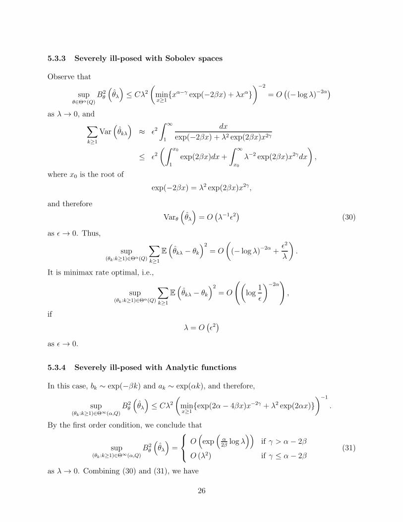
5.3.3 Severely ill-posed with Sobolev spaces
Observe that
supθ∈Θα(Q)
B2θ
(
θλ
)
≤ Cλ2(
minx≥1
{xα−γ exp(−2βx) + λxα}
)−2
= O(
(− log λ)−2α)
as λ→ 0, and
∑
k≥1
Var(
θkλ
)
≈ ǫ2∫ ∞
1
dx
exp(−2βx) + λ2 exp(2βx)x2γ
≤ ǫ2(∫ x0
1
exp(2βx)dx+
∫ ∞
x0
λ−2 exp(2βx)x2γdx
)
,
where x0 is the root of
exp(−2βx) = λ2 exp(2βx)x2γ,
and therefore
Varθ
(
θλ
)
= O(
λ−1ǫ2)
(30)
as ǫ→ 0. Thus,
sup(θk:k≥1)∈Θα(Q)
∑
k≥1
E
(
θkλ − θk
)2
= O
(
(− log λ)−2α +ǫ2
λ
)
.
It is minimax rate optimal, i.e.,
sup(θk :k≥1)∈Θα(Q)
∑
k≥1
E
(
θkλ − θk
)2
= O
(
(
log1
ǫ
)−2α)
,
if
λ = O(
ǫ2)
as ǫ→ 0.
5.3.4 Severely ill-posed with Analytic functions
In this case, bk ∼ exp(−βk) and ak ∼ exp(αk), and therefore,
sup(θk :k≥1)∈Θ∞(α,Q)
B2θ
(
θλ
)
≤ Cλ2(
minx≥1
{exp(2α− 4βx)x−2γ + λ2 exp(2αx)}
)−1
.
By the first order condition, we conclude that
sup(θk :k≥1)∈Θ∞(α,Q)
B2θ
(
θλ
)
=
O(
exp(
α2β
log λ))
if γ > α− 2β
O (λ2) if γ ≤ α− 2β(31)
as λ→ 0. Combining (30) and (31), we have
26

(a) if γ ≥ α− 2β,
sup(θk:k≥1)∈Θ∞(α,Q)
∑
k≥1
E
(
θkλ − θk
)2
= O
(
exp
(
α
2βlog λ
)
+ λ−1ǫ2)
. (32)
The best achievable rate is
sup(θk:k≥1)∈Θ∞(α,Q)
∑
k≥1
E
(
θkλ − θk
)2
= O(
ǫ2α
α+2β
)
,
and it can be attained when
λ = O(
ǫ4β
α+2β
)
as ǫ→ 0 ;
(b) if γ < α− 2β,
sup(θk :k≥1)∈Θ∞(α,Q)
∑
k≥1
E
(
θkλ − θk
)2
= O(
λ2 + λ−1ǫ2)
.
The best achievable rate is
sup(θk:k≥1)∈Θ∞(α,Q)
∑
k≥1
E
(
θkλ − θk
)2
= O(
ǫ43
)
and it is attained when
λ = O(
ǫ43
)
as ǫ→ 0.
References
[1] Aronszajn, N. (1950). Theory of reproducing kernels. Transactions of the American
Mathematical Society, 68 (3), 337-404.
[2] Brown, L. D. and Low, M. G. (1996). Asymptotic equivalence of nonparametric regres-
sion and white noise. Annals of Statististics, 24, 2384-2398.
[3] Buhmann, M. D. (2003). Radial Basis Functions: Theory and Implementations. Cam-
bridge: University Press.
27
[4] Cavalier, L. (2008). Nonparametric statistical inverse problems. Inverse Problems, 24,
1-19.
[5] Chalmond, B. (2008). Modeling and Inverse Problems in Image Analysis. New York:
Springer.
[6] Evgeniou, T., Pontil, M., and Poggio,T. (2000). Statistical Learning Theory: A Primer.
International Journal of Computer Vision, 38 (1), 9-13.
[7] Girosi, F., Jones, M. and Poggio, T. (1993). Priors, stabilizers and basis functions: From
regularization to radial, tensor and additive splines. Artificial Intelligence memo 1430,
MIT, Artificial Intelligence Laboratory.
[8] Golubev, G. and Nussbaum, M. (1998). Asymptotic equivalence of spectral density and
regression estimation. Technical report, Weierstrass Institute for Applied Analysis and
Stochastics, Berlin.
[9] Grama, I. and Nussbaum, M. (1997). Asymptotic equivalence for nonparametric gen-
eralized linear models. Technical report, Weierstrass Institute for Applied Analysis and
Stochastics, Berlin.
[10] Johnstone, I. (1998). Function Estimation and Gaussian Sequence Models. Unpublished
manuscript.
[11] Kaipo, J. and Somersalo, E. (2004). Statistical and Computational Inverse Problems.
New York: Springer.
[12] Lin, Y. and Brown, L. (2004). Statistical properties of the method of regularization with
periodic Gaussian reproducing kernel, Annals of Statistics, 32, 1723-1743.
[13] Lin, Y. and Yuan, M. (2006). Convergence rates of compactly supported radial basis
function regularization. Statistica Sinica, 16, 425-439.
[14] Nussbaum, M. (1996). Asymptotic equivalence of density estimation and Gaussian white
noise. Annals of Statististics, 24, 2399-2430.
[15] Ramm, A. (2009). Inverse Problems: Mathematical and Analytical Techniques with Ap-
plications to Engineering. New York: Springer.
28
[16] Shi, T. and Yu, B. (2005). Binning in Gaussian Kernel Regularization. Statistica Sinica
16, 541-567.
[17] Smola, A., Scholkopf, B. and Muller, K.R. (1998). The connection between regulariza-
tion operators and support vector kernels. Neural Networks, 11, 637-649.
[18] Wahba, G. (1990). Spline Models for Observational Data. Philadelphia: SIAM.
[19] Wahba, G. (1999). Support vector machines, reproducing kernel Hilbert spaces and the
randomized GACV. In B. Scholkopf, C. Burges & A. Smola, eds, Advances in Kernel
Methods Support Vector Learning. Cambridge: MIT Press, 69-88
[20] Wendland, H. (1998). Error estimates for interpolation by compactly supported radial
basis functions of minimal degree. Journal of Approximation Theory, 93, 258-272.
[21] Zhang, H., Genton, M. and Liu, P. (2004). Compactly supported radial basis function
kernels. Institute of Statistics Mimeo Series 2570, North Carolina State University.
29