
18 GeneralRVs-3 Gaussian
77
3. General Random Variables Part III: Normal (Gaussian) Random Variable ECE 302 Spring 2012 Purdue University, School of ECE Prof. Ilya Pollak
description
guassian revo2
Transcript of 18 GeneralRVs-3 Gaussian

3. General Random Variables Part III: Normal (Gaussian) Random
Variable
ECE 302 Spring 2012 Purdue University, School of ECE
Prof. Ilya Pollak
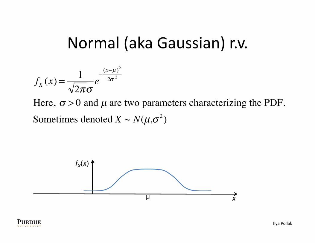
Normal (aka Gaussian) r.v.
�
fX (x) = 12πσ
e− (x−µ )2
2σ 2
Here, σ > 0 and µ are two parameters characterizing the PDF.Sometimes denoted X ~ N(µ,σ 2)
x
fX(x)
µ
Ilya Pollak
NormalizaKon fX (x) = 1
2πσe−
(x−µ )2
2σ 2
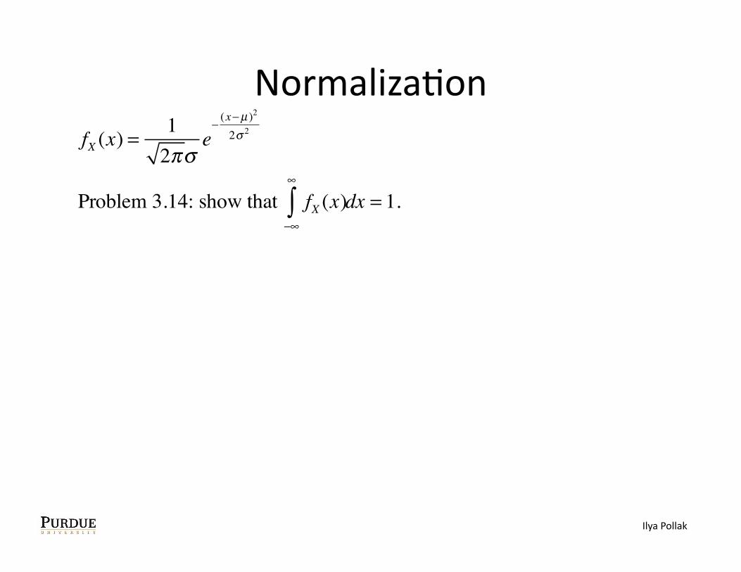
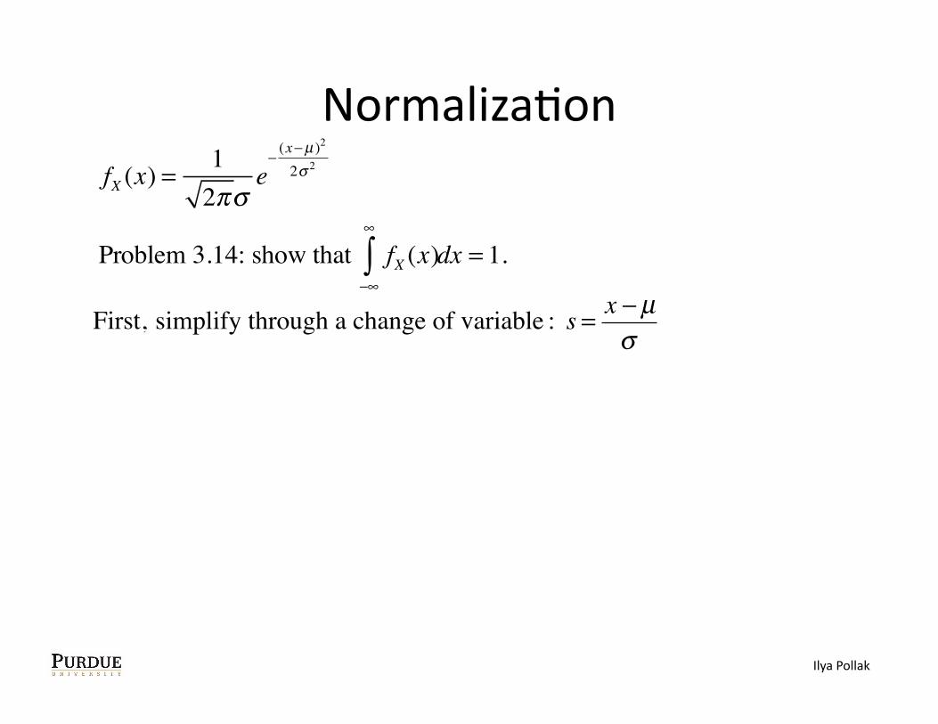
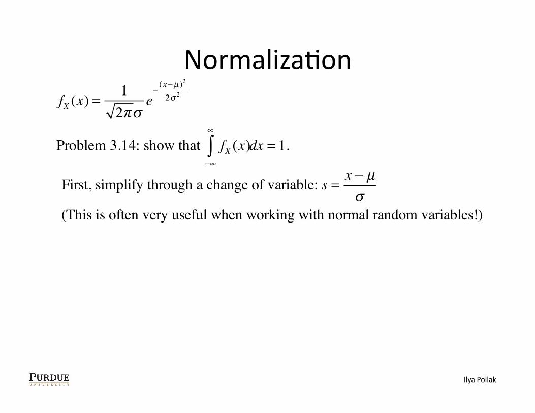
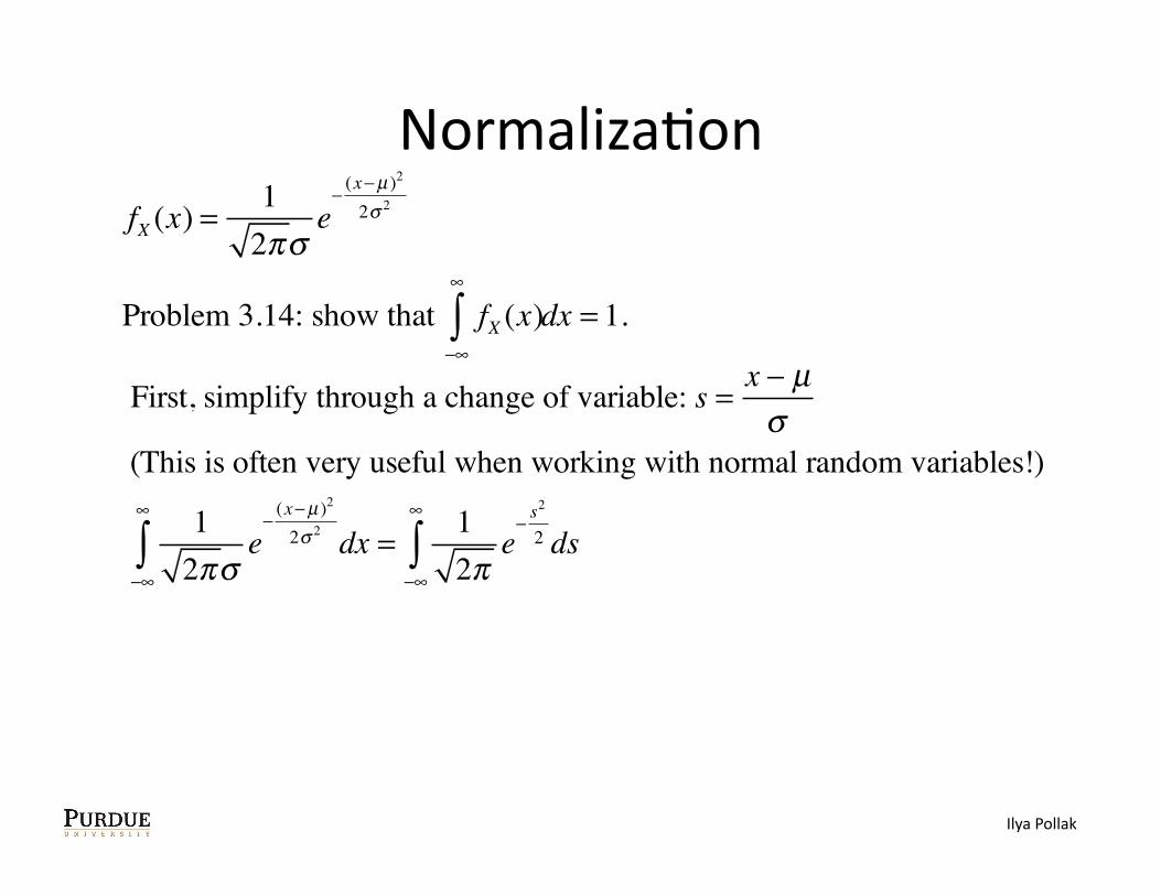
Problem 3.14: show that fX (x)−∞
∞
∫ dx = 1.
Ilya Pollak
NormalizaKon fX (x) = 1
2πσe−
(x−µ )2
2σ 2
Problem 3.14: show that fX (x)−∞
∞
∫ dx = 1.
�
First, simplify through a change of variable : s = x − µσ
Ilya Pollak
NormalizaKon fX (x) = 1
2πσe−
(x−µ )2
2σ 2
Problem 3.14: show that fX (x)−∞
∞
∫ dx = 1.
First, simplify through a change of variable: s = x − µσ
(This is often very useful when working with normal random variables!)
Ilya Pollak
NormalizaKon fX (x) = 1
2πσe−
(x−µ )2
2σ 2
Problem 3.14: show that fX (x)−∞
∞
∫ dx = 1.
First, simplify through a change of variable: s = x − µσ
(This is often very useful when working with normal random variables!)
12πσ
e−
(x−µ )2
2σ 2
−∞
∞
∫ dx = 12π
e−s2
2
−∞
∞
∫ ds
Ilya Pollak
NormalizaKon fX (x) = 1
2πσe−
(x−µ )2
2σ 2
Problem 3.14: show that fX (x)−∞
∞
∫ dx = 1.
First, simplify through a change of variable: s = x − µσ
(This is often very useful when working with normal random variables!)
12πσ
e−
(x−µ )2
2σ 2
−∞
∞
∫ dx = 12π
e−s2
2
−∞
∞
∫ ds
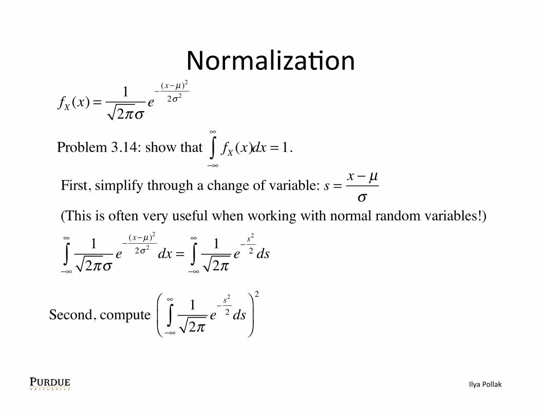
Second, compute 12π
e−s2
2
−∞
∞
∫ ds⎛
⎝⎜
⎞
⎠⎟
2
Ilya Pollak
NormalizaKon fX (x) = 1
2πσe−
(x−µ )2
2σ 2
Problem 3.14: show that fX (x)−∞
∞
∫ dx = 1.
First, simplify through a change of variable: s = x − µσ
(This is often very useful when working with normal random variables!)
12πσ
e−
(x−µ )2
2σ 2
−∞
∞
∫ dx = 12π
e−s2
2
−∞
∞
∫ ds
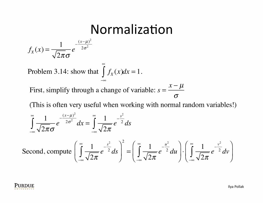
Second, compute 12π
e−s2
2
−∞
∞
∫ ds⎛
⎝⎜
⎞
⎠⎟
2
=12π
e−u2
2
−∞
∞
∫ du⎛
⎝⎜
⎞
⎠⎟ ⋅
12π
e−v2
2
−∞
∞
∫ dv⎛
⎝⎜
⎞
⎠⎟
Ilya Pollak
NormalizaKon fX (x) = 1
2πσe−
(x−µ )2
2σ 2
Problem 3.14: show that fX (x)−∞
∞
∫ dx = 1.
First, simplify through a change of variable: s = x − µσ
(This is often very useful when working with normal random variables!)
12πσ
e−
(x−µ )2
2σ 2
−∞
∞
∫ dx = 12π
e−s2
2
−∞
∞
∫ ds
Second, compute 12π
e−s2
2
−∞
∞
∫ ds⎛
⎝⎜
⎞
⎠⎟
2
=12π
e−u2
2
−∞
∞
∫ du⎛
⎝⎜
⎞
⎠⎟ ⋅
12π
e−v2
2
−∞
∞
∫ dv⎛
⎝⎜
⎞
⎠⎟
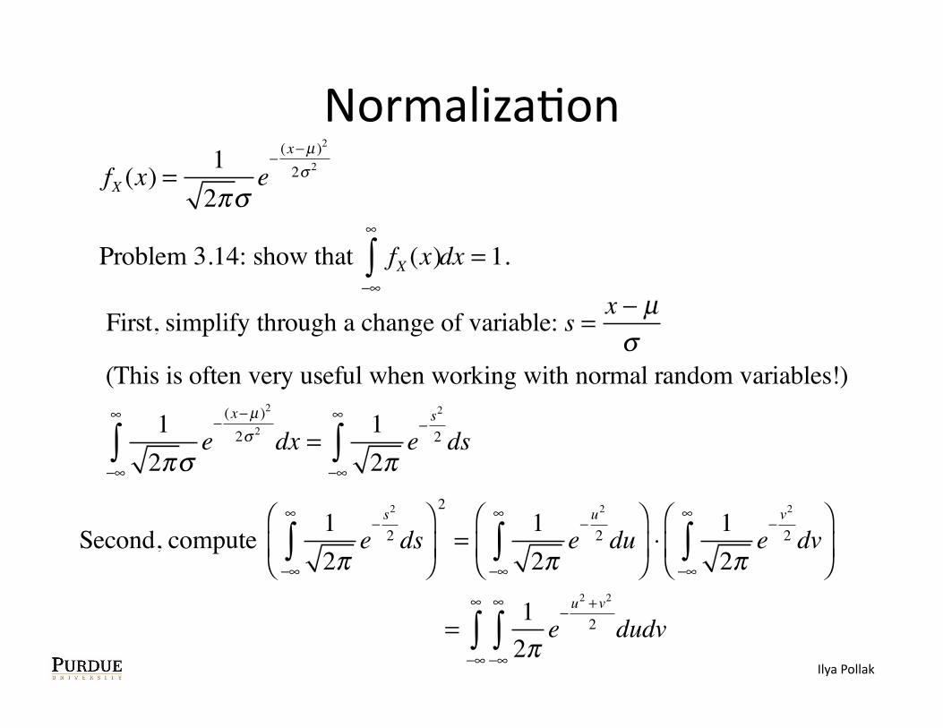
= 12π
e−u2 +v2
2
−∞
∞
∫−∞
∞
∫ dudvIlya Pollak
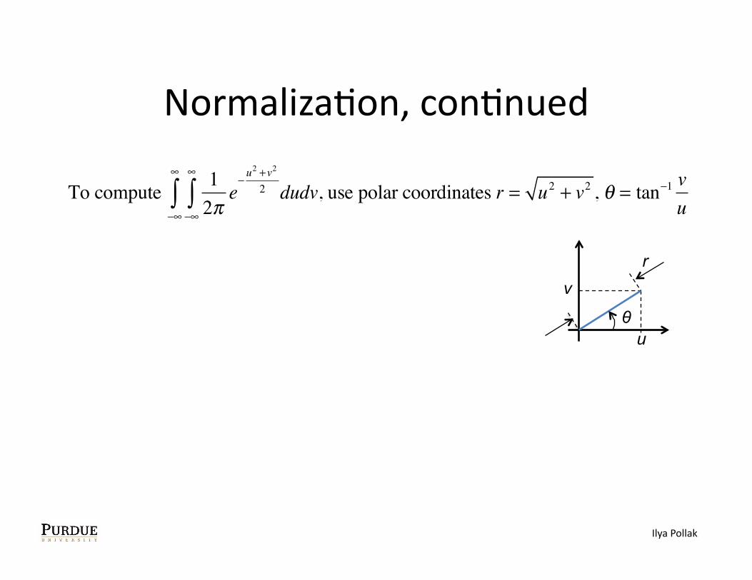
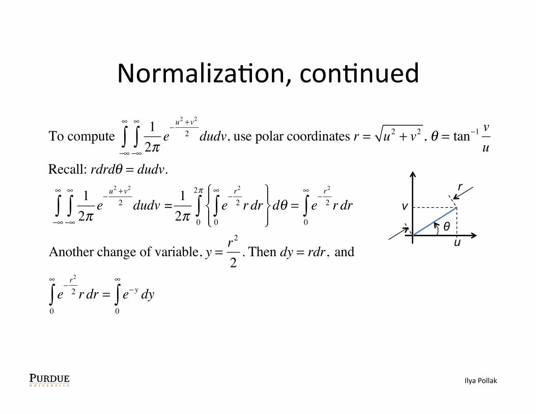
NormalizaKon, conKnued
To compute 12π
e−u2 +v2
2
−∞
∞
∫−∞
∞
∫ dudv, use polar coordinates r = u2 + v2 , θ = tan−1 vu
v
u θ
r
Ilya Pollak
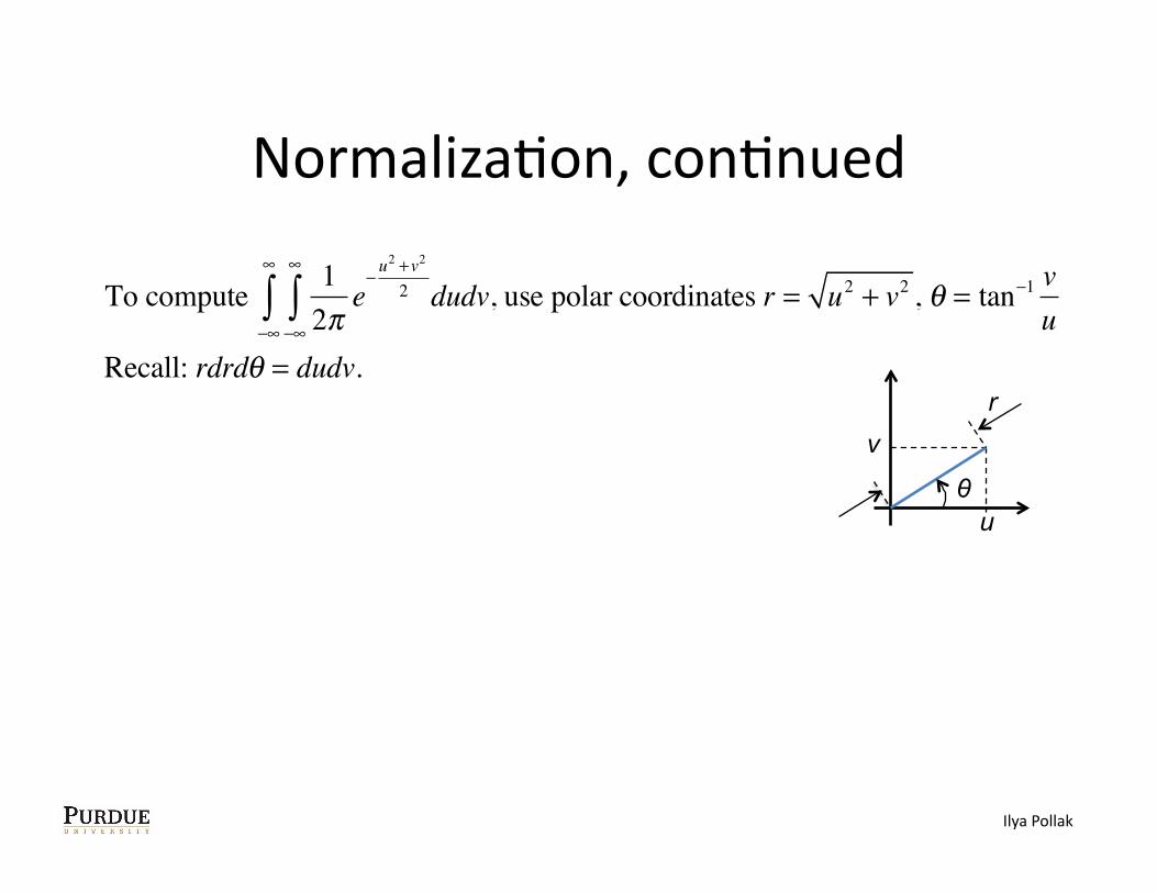
NormalizaKon, conKnued
To compute 12π
e−u2 +v2
2
−∞
∞
∫−∞
∞
∫ dudv, use polar coordinates r = u2 + v2 , θ = tan−1 vu
Recall: rdrdθ = dudv.
v
u θ
r
Ilya Pollak

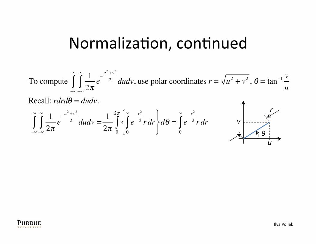
NormalizaKon, conKnued
To compute 12π
e−u2 +v2
2
−∞
∞
∫−∞
∞
∫ dudv, use polar coordinates r = u2 + v2 , θ = tan−1 vu
Recall: rdrdθ = dudv.
12π
e−u2 +v2
2
−∞
∞
∫−∞
∞
∫ dudv = 12π
e−r2
2 r dr0
∞
∫⎧⎨⎪
⎩⎪
⎫⎬⎪
⎭⎪dθ
0
2π
∫ v
u θ
r
Ilya Pollak
NormalizaKon, conKnued
To compute 12π
e−u2 +v2
2
−∞
∞
∫−∞
∞
∫ dudv, use polar coordinates r = u2 + v2 , θ = tan−1 vu
Recall: rdrdθ = dudv.
12π
e−u2 +v2
2
−∞
∞
∫−∞
∞
∫ dudv = 12π
e−r2
2 r dr0
∞
∫⎧⎨⎪
⎩⎪
⎫⎬⎪
⎭⎪dθ
0
2π
∫ = e−r2
2 r dr0
∞
∫ v
u θ
r
Ilya Pollak
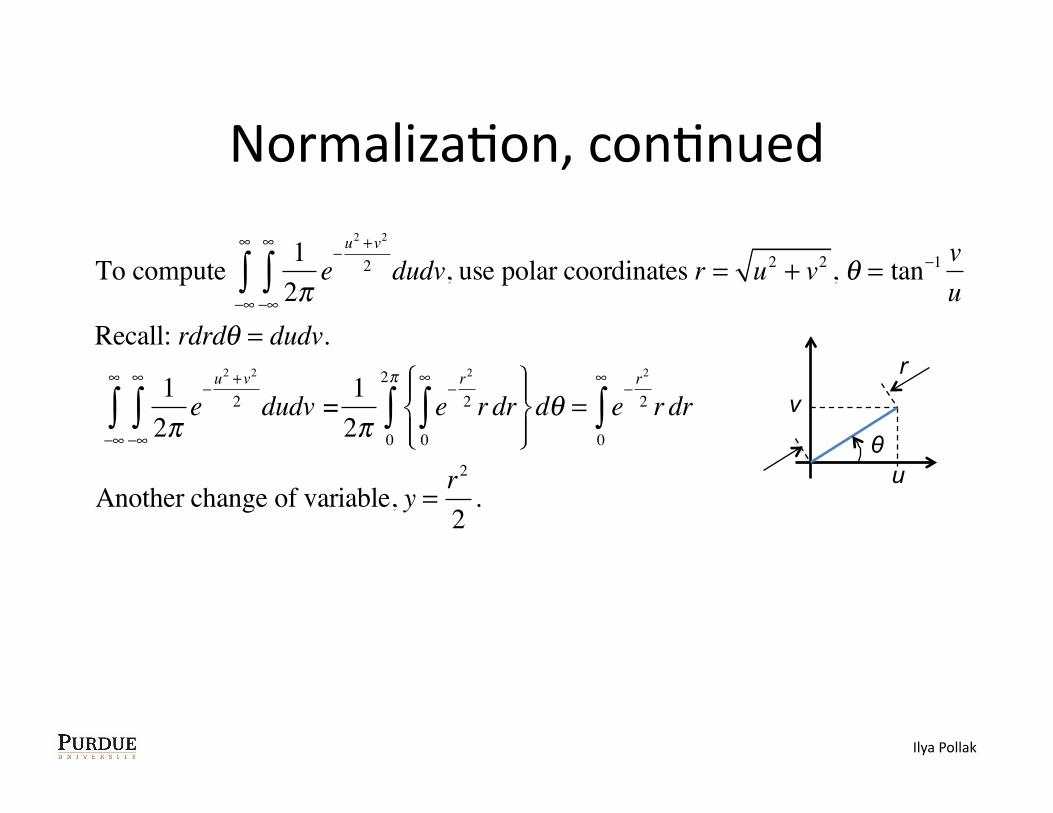
NormalizaKon, conKnued
To compute 12π
e−u2 +v2
2
−∞
∞
∫−∞
∞
∫ dudv, use polar coordinates r = u2 + v2 , θ = tan−1 vu
Recall: rdrdθ = dudv.
12π
e−u2 +v2
2
−∞
∞
∫−∞
∞
∫ dudv = 12π
e−r2
2 r dr0
∞
∫⎧⎨⎪
⎩⎪
⎫⎬⎪
⎭⎪dθ
0
2π
∫ = e−r2
2 r dr0
∞
∫
Another change of variable, y = r2
2.
v
u θ
r
Ilya Pollak
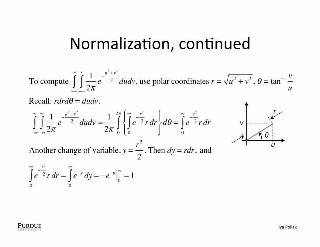
NormalizaKon, conKnued
To compute 12π
e−u2 +v2
2
−∞
∞
∫−∞
∞
∫ dudv, use polar coordinates r = u2 + v2 , θ = tan−1 vu
Recall: rdrdθ = dudv.
12π
e−u2 +v2
2
−∞
∞
∫−∞
∞
∫ dudv = 12π
e−r2
2 r dr0
∞
∫⎧⎨⎪
⎩⎪
⎫⎬⎪
⎭⎪dθ
0
2π
∫ = e−r2
2 r dr0
∞
∫
Another change of variable, y = r2
2. Then dy = rdr, and
e−r2
2 r dr0
∞
∫ = e− y dy0
∞
∫
v
u θ
r
Ilya Pollak
NormalizaKon, conKnued
To compute 12π
e−u2 +v2
2
−∞
∞
∫−∞
∞
∫ dudv, use polar coordinates r = u2 + v2 , θ = tan−1 vu
Recall: rdrdθ = dudv.
12π
e−u2 +v2
2
−∞
∞
∫−∞
∞
∫ dudv = 12π
e−r2
2 r dr0
∞
∫⎧⎨⎪
⎩⎪
⎫⎬⎪
⎭⎪dθ
0
2π
∫ = e−r2
2 r dr0
∞
∫
Another change of variable, y = r2
2. Then dy = rdr, and
e−r2
2 r dr0
∞
∫ = e− y dy = −e−u0
∞= 1
0
∞
∫
v
u θ
r
Ilya Pollak
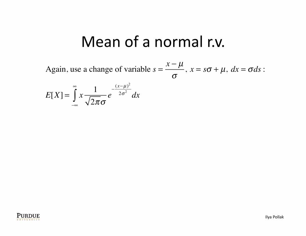
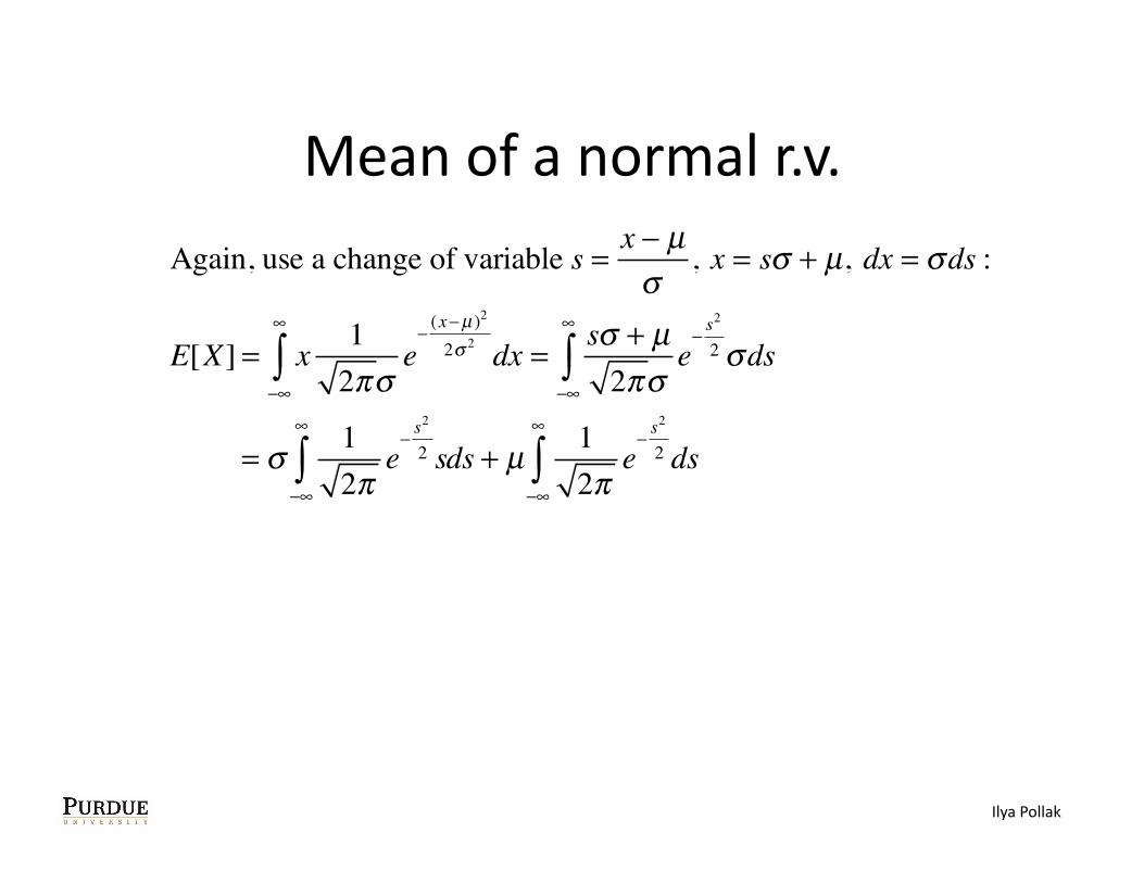
Mean of a normal r.v.
Again, use a change of variable s = x − µσ
, x = sσ + µ, dx = σds :
E[X] = x 12πσ
e−
(x−µ )2
2σ 2
−∞
∞
∫ dx
Ilya Pollak
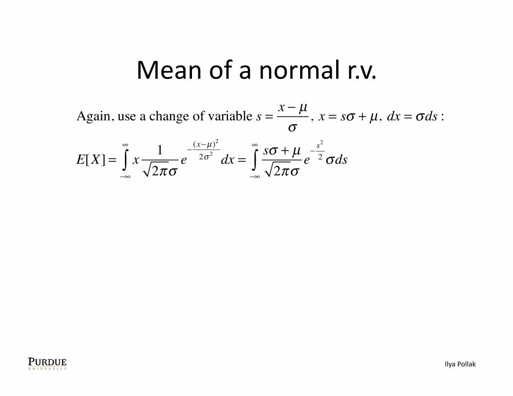
Mean of a normal r.v.
Again, use a change of variable s = x − µσ
, x = sσ + µ, dx = σds :
E[X] = x 12πσ
e−
(x−µ )2
2σ 2
−∞
∞
∫ dx = sσ + µ2πσ
e−s2
2
−∞
∞
∫ σds
Ilya Pollak
Mean of a normal r.v.
Again, use a change of variable s = x − µσ
, x = sσ + µ, dx = σds :
E[X] = x 12πσ
e−
(x−µ )2
2σ 2
−∞
∞
∫ dx = sσ + µ2πσ
e−s2
2
−∞
∞
∫ σds
= σ 12π
e−s2
2 s−∞
∞
∫ ds + µ 12π
e−s2
2
−∞
∞
∫ ds
Ilya Pollak
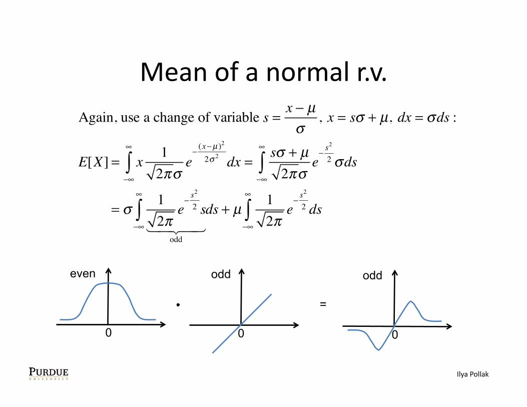
Mean of a normal r.v. Again, use a change of variable s = x − µ
σ, x = sσ + µ, dx = σds :
E[X] = x 12πσ
e−
(x−µ )2
2σ 2
−∞
∞
∫ dx = sσ + µ2πσ
e−s2
2
−∞
∞
∫ σds
= σ 12π
e−s2
2 s
odd −∞
∞
∫ ds + µ 12π
e−s2
2
−∞
∞
∫ ds
even
0
odd
0
odd
0
=
Ilya Pollak
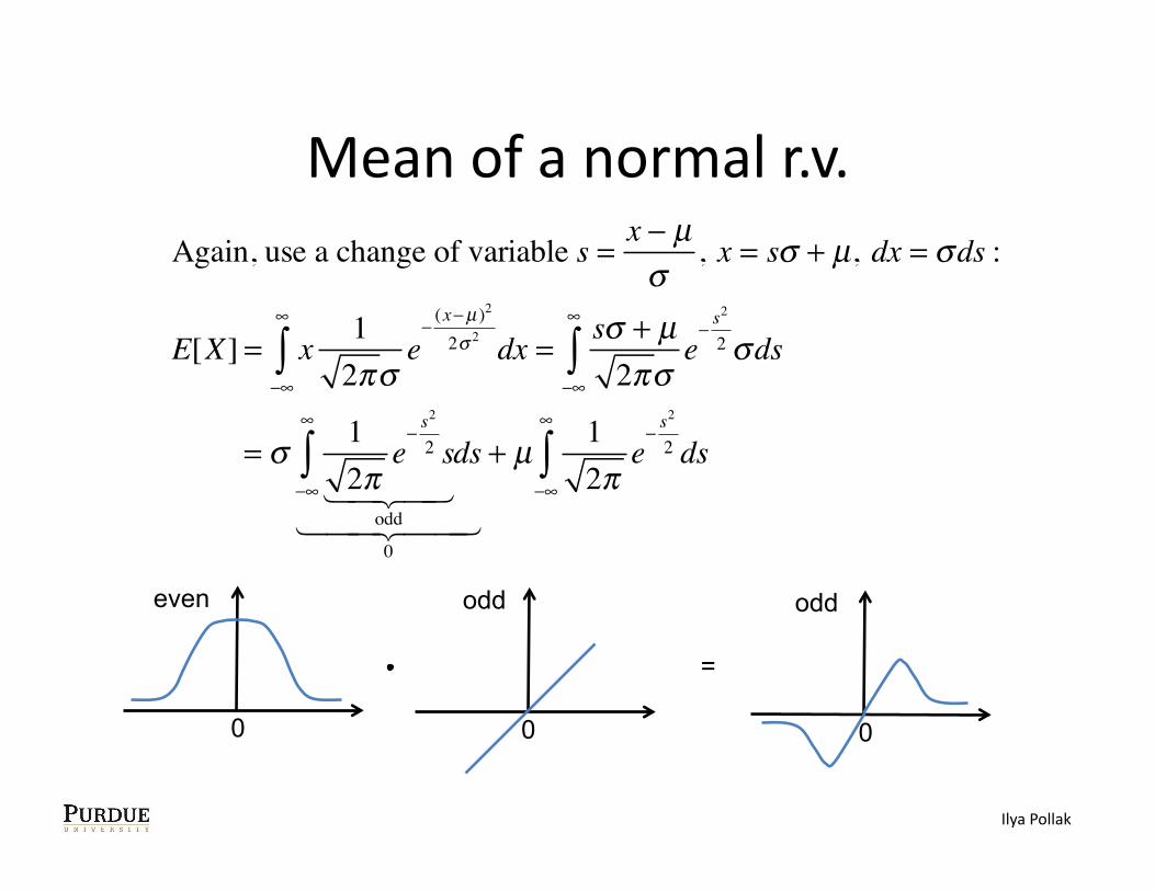
Mean of a normal r.v. Again, use a change of variable s = x − µ
σ, x = sσ + µ, dx = σds :
E[X] = x 12πσ
e−
(x−µ )2
2σ 2
−∞
∞
∫ dx = sσ + µ2πσ
e−s2
2
−∞
∞
∫ σds
= σ 12π
e−s2
2 s
odd −∞
∞
∫ ds
0
+ µ 12π
e−s2
2
−∞
∞
∫ ds
even
0
odd
0
odd
0
=
Ilya Pollak

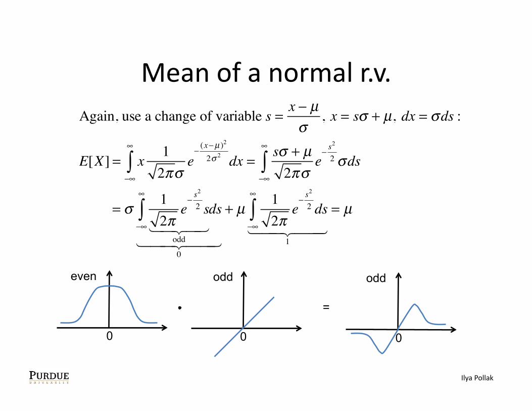
Mean of a normal r.v. Again, use a change of variable s = x − µ
σ, x = sσ + µ, dx = σds :
E[X] = x 12πσ
e−
(x−µ )2
2σ 2
−∞
∞
∫ dx = sσ + µ2πσ
e−s2
2
−∞
∞
∫ σds
= σ 12π
e−s2
2 s
odd −∞
∞
∫ ds
0
+ µ 12π
e−s2
2
−∞
∞
∫ ds
1
even
0
odd
0
odd
0
=
Ilya Pollak
Mean of a normal r.v. Again, use a change of variable s = x − µ
σ, x = sσ + µ, dx = σds :
E[X] = x 12πσ
e−
(x−µ )2
2σ 2
−∞
∞
∫ dx = sσ + µ2πσ
e−s2
2
−∞
∞
∫ σds
= σ 12π
e−s2
2 s
odd −∞
∞
∫ ds
0
+ µ 12π
e−s2
2
−∞
∞
∫ ds
1
= µ
even
0
odd
0
odd
0
=
Ilya Pollak

Normal PDF is symmetric around the mean
�
fX (µ + u) = 12πσ
e− u2
2σ 2 = fX (µ − u)
fX (x) =12πσ
e−(x−µ )2
2σ 2
Ilya Pollak

The maximum of a normal PDF is at its mean
�
′ f X (x) = − x − µσ 2
12πσ
e− (x−µ )2
2σ 2
�
fX (x) = 12πσ
e− (x−µ )2
2σ 2
Ilya Pollak

The maximum of a normal PDF is at its mean
�
′ f X (x) = − x − µσ 2
12πσ
e− (x−µ )2
2σ 2
Unique extremum is at x = µ.Since ′ f X (x) > 0 for x < µ and ′ f X (x) < 0 for x > µ,it's a maximum.
�
fX (x) = 12πσ
e− (x−µ )2
2σ 2
Ilya Pollak
The variance and standard deviaKon of a normal r.v.
• Variance = σ2 • Standard deviaKon = σ • Exercise: integraKon by parts
�
fX (x) = 12πσ
e− (x−µ )2
2σ 2
Ilya Pollak
A linear funcKon of a normal r.v. is a normal r.v.
• Suppose X is normal with mean μ and variance σ2, and a ≠ 0, b are real numbers
Ilya Pollak
A linear funcKon of a normal r.v. is a normal r.v.
• Suppose X is normal with mean μ and variance σ2, and a ≠ 0, b are real numbers
• Let Y = aX + b
Ilya Pollak
A linear funcKon of a normal r.v. is a normal r.v.
• Suppose X is normal with mean μ and variance σ2, and a ≠ 0, b are real numbers
• Let Y = aX + b • Then Y is a normal random variable
Ilya Pollak
A linear funcKon of a normal r.v. is a normal r.v.
• Suppose X is normal with mean μ and variance σ2, and a ≠ 0, b are real numbers
• Let Y = aX + b • Then Y is a normal random variable
• E[Y] = aμ + b
Ilya Pollak
A linear funcKon of a normal r.v. is a normal r.v.
• Suppose X is normal with mean μ and variance σ2, and a ≠ 0, b are real numbers
• Let Y = aX + b • Then Y is a normal random variable
• E[Y] = aμ + b • var(Y) = a2σ2
Ilya Pollak
A linear funcKon of a normal r.v. is a normal r.v.
�
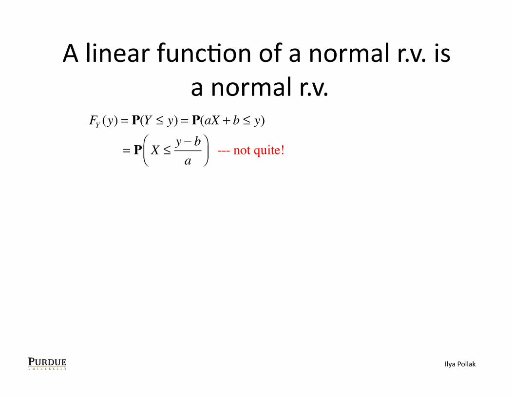
FY (y) = P(Y ≤ y) = P(aX + b ≤ y)
Ilya Pollak
A linear funcKon of a normal r.v. is a normal r.v.
FY (y) = P(Y ≤ y) = P(aX + b ≤ y)
= P X ≤y − ba
⎛⎝⎜
⎞⎠⎟
Ilya Pollak
A linear funcKon of a normal r.v. is a normal r.v.
FY (y) = P(Y ≤ y) = P(aX + b ≤ y)
= P X ≤y − ba
⎛⎝⎜
⎞⎠⎟
--- not quite!
Ilya Pollak
A linear funcKon of a normal r.v. is a normal r.v.
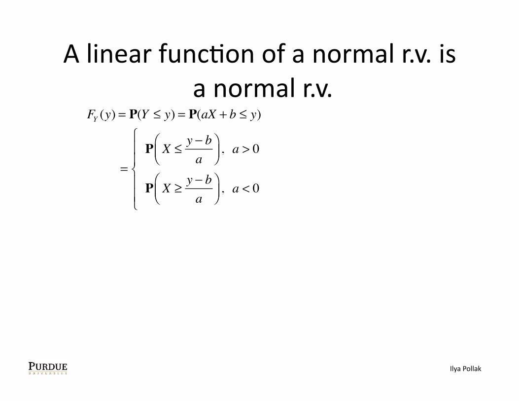
FY (y) = P(Y ≤ y) = P(aX + b ≤ y)
=P X ≤
y − ba
⎛⎝⎜
⎞⎠⎟
, a > 0
P X ≥y − ba
⎛⎝⎜
⎞⎠⎟
, a < 0
⎧
⎨⎪⎪
⎩⎪⎪
Ilya Pollak
A linear funcKon of a normal r.v. is a normal r.v.
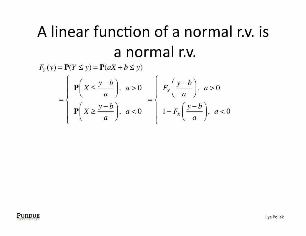
FY (y) = P(Y ≤ y) = P(aX + b ≤ y)
=P X ≤
y − ba
⎛⎝⎜
⎞⎠⎟
, a > 0
P X ≥y − ba
⎛⎝⎜
⎞⎠⎟
, a < 0
⎧
⎨⎪⎪
⎩⎪⎪
=FX
y − ba
⎛⎝⎜
⎞⎠⎟
, a > 0
1− FXy − ba
⎛⎝⎜
⎞⎠⎟
, a < 0
⎧
⎨⎪⎪
⎩⎪⎪
Ilya Pollak
A linear funcKon of a normal r.v. is a normal r.v.
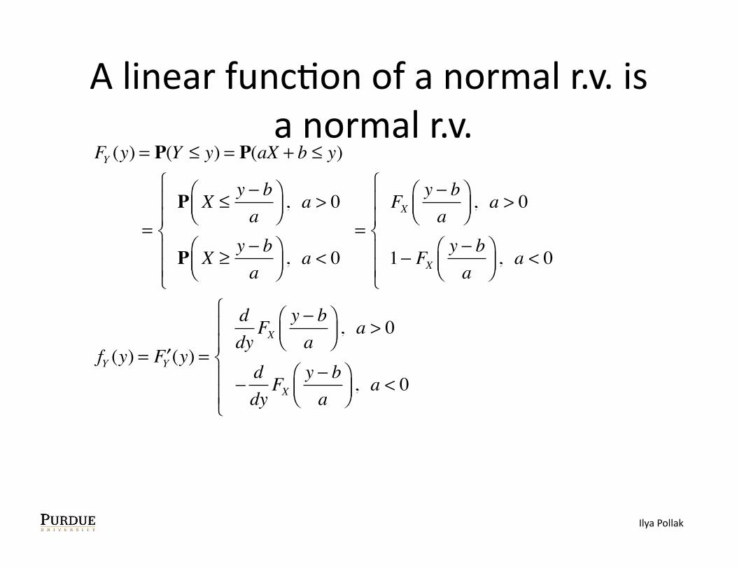
FY (y) = P(Y ≤ y) = P(aX + b ≤ y)
=P X ≤
y − ba
⎛⎝⎜
⎞⎠⎟
, a > 0
P X ≥y − ba
⎛⎝⎜
⎞⎠⎟
, a < 0
⎧
⎨⎪⎪
⎩⎪⎪
=FX
y − ba
⎛⎝⎜
⎞⎠⎟
, a > 0
1− FXy − ba
⎛⎝⎜
⎞⎠⎟
, a < 0
⎧
⎨⎪⎪
⎩⎪⎪
fY (y) = ′FY (y) =
ddyFX
y − ba
⎛⎝⎜
⎞⎠⎟
, a > 0
−ddyFX
y − ba
⎛⎝⎜
⎞⎠⎟
, a < 0
⎧
⎨
⎪⎪
⎩
⎪⎪
Ilya Pollak
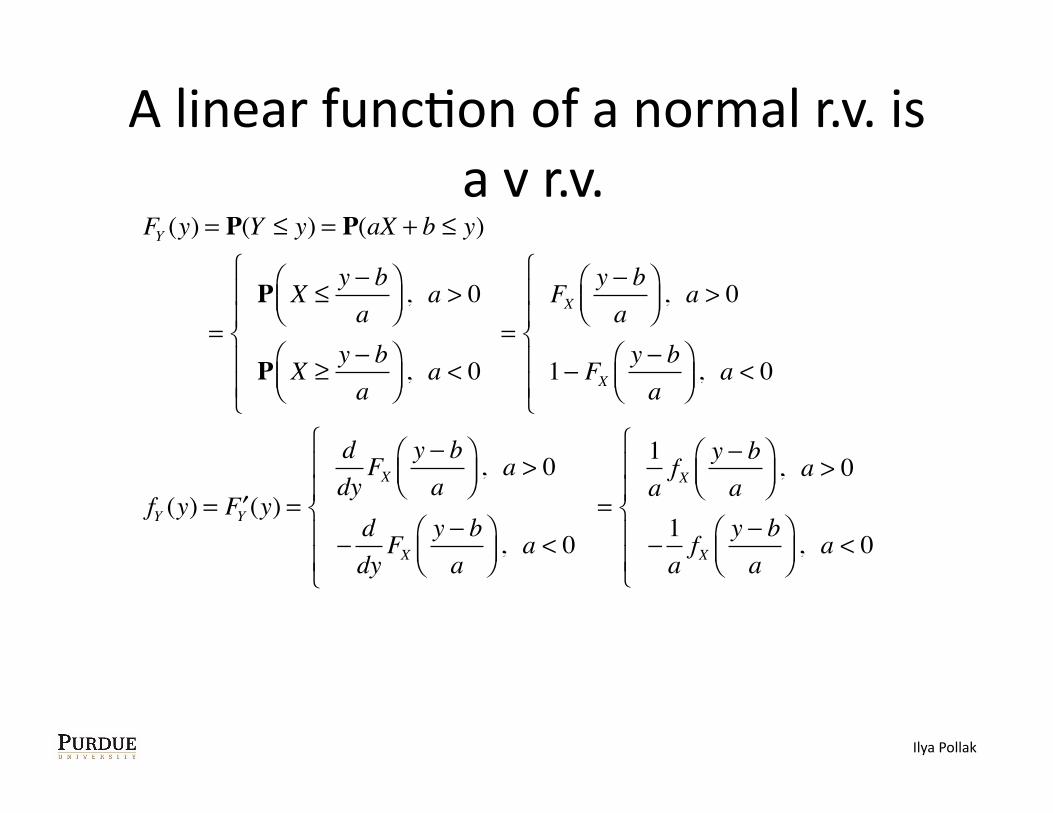
A linear funcKon of a normal r.v. is a v r.v.
FY (y) = P(Y ≤ y) = P(aX + b ≤ y)
=P X ≤
y − ba
⎛⎝⎜
⎞⎠⎟
, a > 0
P X ≥y − ba
⎛⎝⎜
⎞⎠⎟
, a < 0
⎧
⎨⎪⎪
⎩⎪⎪
=FX
y − ba
⎛⎝⎜
⎞⎠⎟
, a > 0
1− FXy − ba
⎛⎝⎜
⎞⎠⎟
, a < 0
⎧
⎨⎪⎪
⎩⎪⎪
fY (y) = ′FY (y) =
ddyFX
y − ba
⎛⎝⎜
⎞⎠⎟
, a > 0
−ddyFX
y − ba
⎛⎝⎜
⎞⎠⎟
, a < 0
⎧
⎨
⎪⎪
⎩
⎪⎪
=
1afX
y − ba
⎛⎝⎜
⎞⎠⎟
, a > 0
−1afX
y − ba
⎛⎝⎜
⎞⎠⎟
, a < 0
⎧
⎨⎪⎪
⎩⎪⎪
Ilya Pollak
A linear funcKon of a normal r.v. is a normal r.v.
FY (y) = P(Y ≤ y) = P(aX + b ≤ y)
=P X ≤
y − ba
⎛⎝⎜
⎞⎠⎟
, a > 0
P X ≥y − ba
⎛⎝⎜
⎞⎠⎟
, a < 0
⎧
⎨⎪⎪
⎩⎪⎪
=FX
y − ba
⎛⎝⎜
⎞⎠⎟
, a > 0
1− FXy − ba
⎛⎝⎜
⎞⎠⎟
, a < 0
⎧
⎨⎪⎪
⎩⎪⎪
fY (y) = ′FY (y) =
ddyFX
y − ba
⎛⎝⎜
⎞⎠⎟
, a > 0
−ddyFX
y − ba
⎛⎝⎜
⎞⎠⎟
, a < 0
⎧
⎨
⎪⎪
⎩
⎪⎪
=
1afX
y − ba
⎛⎝⎜
⎞⎠⎟
, a > 0
−1afX
y − ba
⎛⎝⎜
⎞⎠⎟
, a < 0
⎧
⎨⎪⎪
⎩⎪⎪
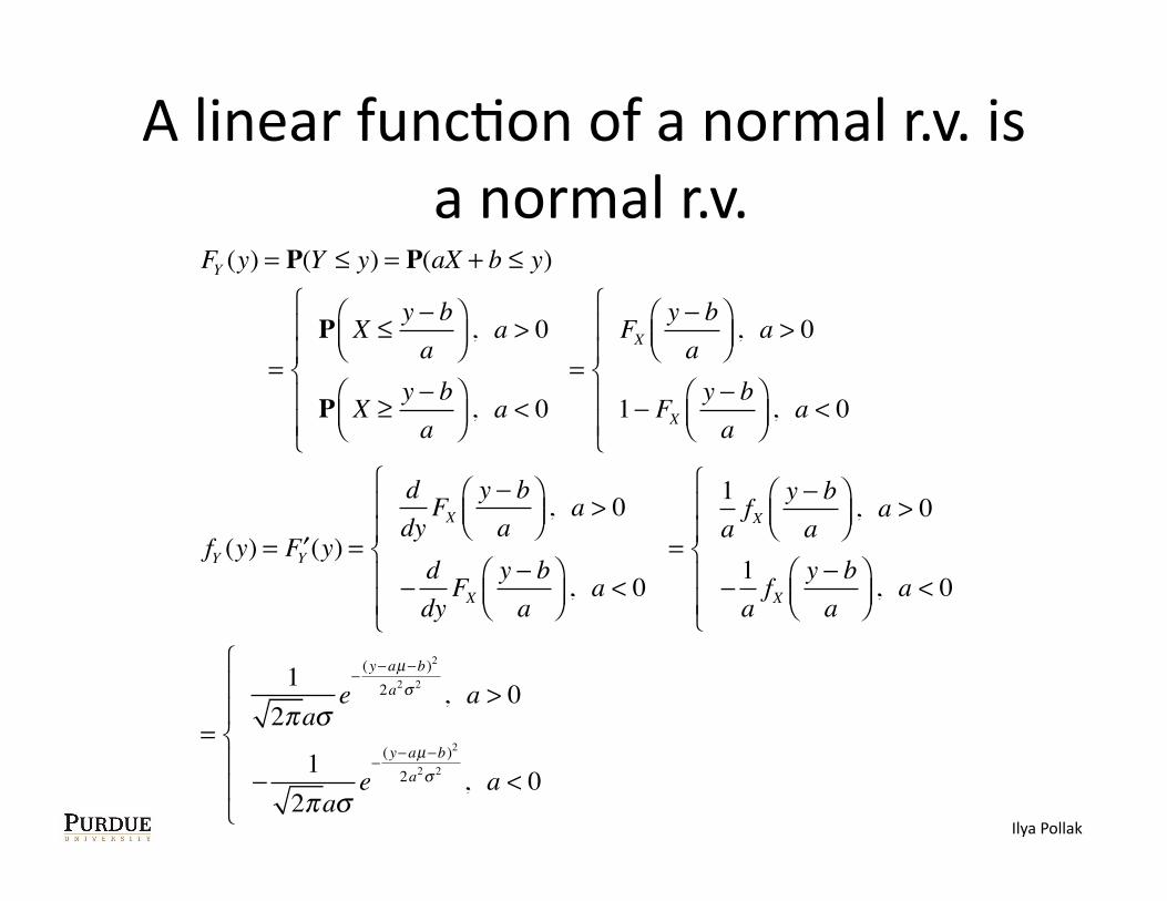
=
12πaσ
e−
(y−aµ−b)2
2a2σ 2 , a > 0
−1
2πaσe−
(y−aµ−b)2
2a2σ 2 , a < 0
⎧
⎨
⎪⎪
⎩
⎪⎪
Ilya Pollak
A linear funcKon of a normal r.v. is a normal r.v.
FY (y) = P(Y ≤ y) = P(aX + b ≤ y)
=P X ≤
y − ba
⎛⎝⎜
⎞⎠⎟
, a > 0
P X ≥y − ba
⎛⎝⎜
⎞⎠⎟
, a < 0
⎧
⎨⎪⎪
⎩⎪⎪
=FX
y − ba
⎛⎝⎜
⎞⎠⎟
, a > 0
1− FXy − ba
⎛⎝⎜
⎞⎠⎟
, a < 0
⎧
⎨⎪⎪
⎩⎪⎪
fY (y) = ′FY (y) =
ddyFX
y − ba
⎛⎝⎜
⎞⎠⎟
, a > 0
−ddyFX
y − ba
⎛⎝⎜
⎞⎠⎟
, a < 0
⎧
⎨
⎪⎪
⎩
⎪⎪
=
1afX
y − ba
⎛⎝⎜
⎞⎠⎟
, a > 0
−1afX
y − ba
⎛⎝⎜
⎞⎠⎟
, a < 0
⎧
⎨⎪⎪
⎩⎪⎪
=
12πaσ
e−
(y−aµ−b)2
2a2σ 2 , a > 0
−1
2πaσe−
(y−aµ−b)2
2a2σ 2 , a < 0
⎧
⎨
⎪⎪
⎩
⎪⎪
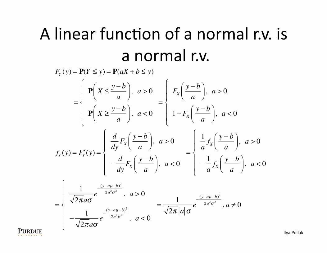
=1
2π a σe−
(y−aµ−b)2
2a2σ 2 , a ≠ 0
Ilya Pollak
Standard normal (aka standard Gaussian) r.v.
• Normal random variable • Mean μ=0
• Standard deviaKon σ=1
Ilya Pollak
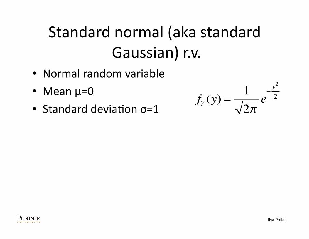
Standard normal (aka standard Gaussian) r.v.
• Normal random variable • Mean μ=0
• Standard deviaKon σ=1 fY (y) =
12π
e−y2
2
Ilya Pollak
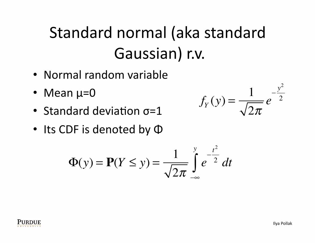
Standard normal (aka standard Gaussian) r.v.
• Normal random variable • Mean μ=0
• Standard deviaKon σ=1 • Its CDF is denoted by Φ
fY (y) =12π
e−y2
2
Φ(y) = P(Y ≤ y) = 12π
e−t2
2 dt−∞
y
∫
Ilya Pollak

How to evaluate normal CDF
• No closed form available for normal CDF
Ilya Pollak

How to evaluate normal CDF
• No closed form available for normal CDF • But there are tables (for standard normal)
Ilya Pollak
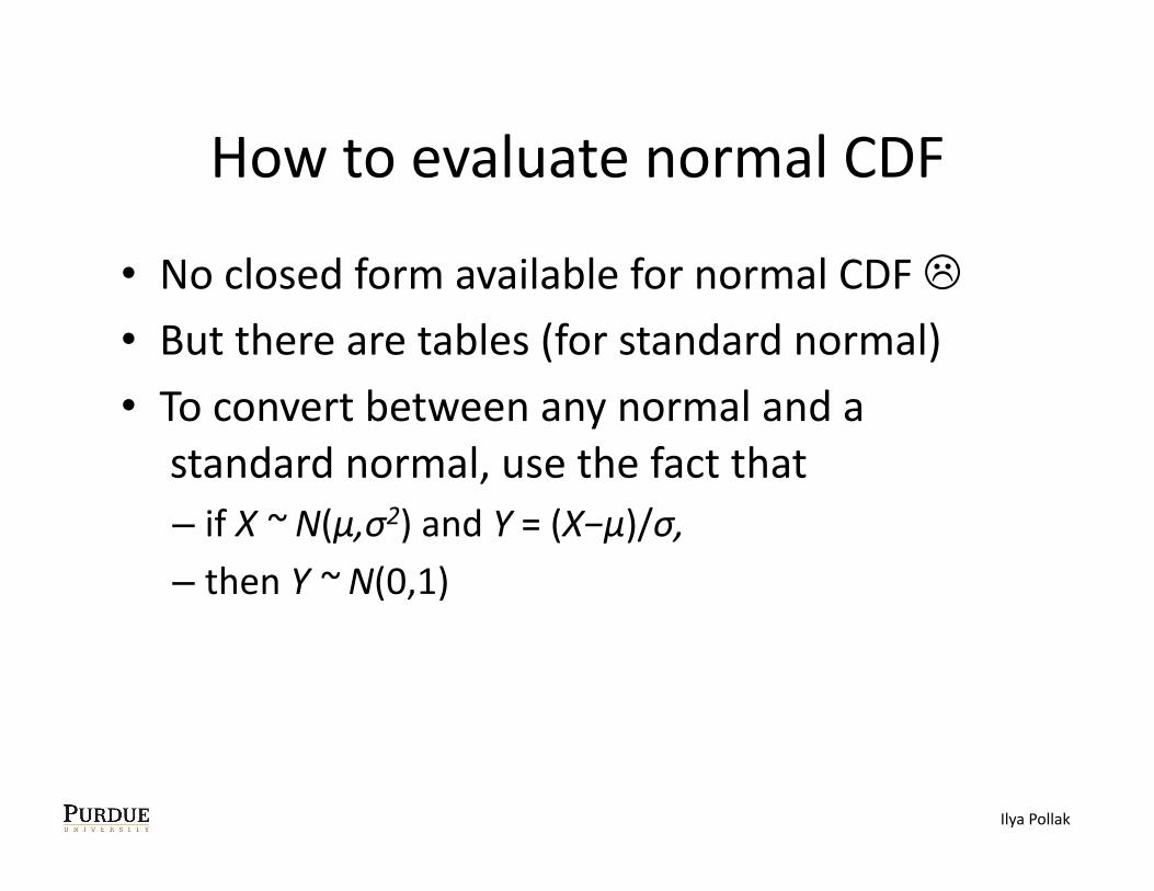
How to evaluate normal CDF
• No closed form available for normal CDF • But there are tables (for standard normal)
• To convert between any normal and a standard normal, use the fact that – if X ~ N(μ,σ2) and Y = (X−μ)/σ, – then Y ~ N(0,1)
Ilya Pollak

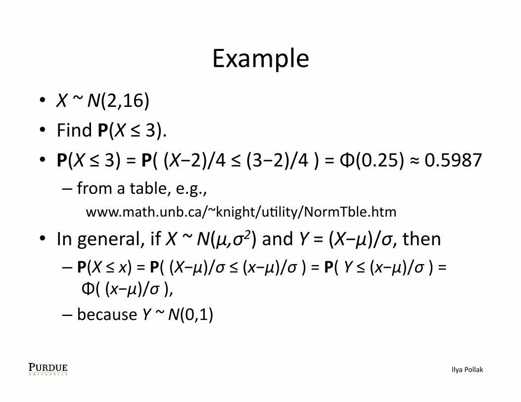
Example • X ~ N(2,16) • Find P(X ≤ 3).
Ilya Pollak
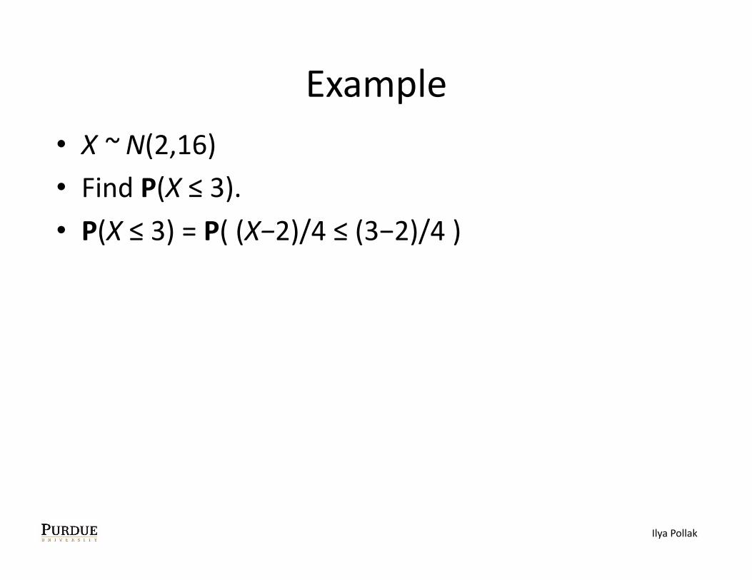
Example • X ~ N(2,16) • Find P(X ≤ 3). • P(X ≤ 3) = P( (X−2)/4 ≤ (3−2)/4 )
Ilya Pollak
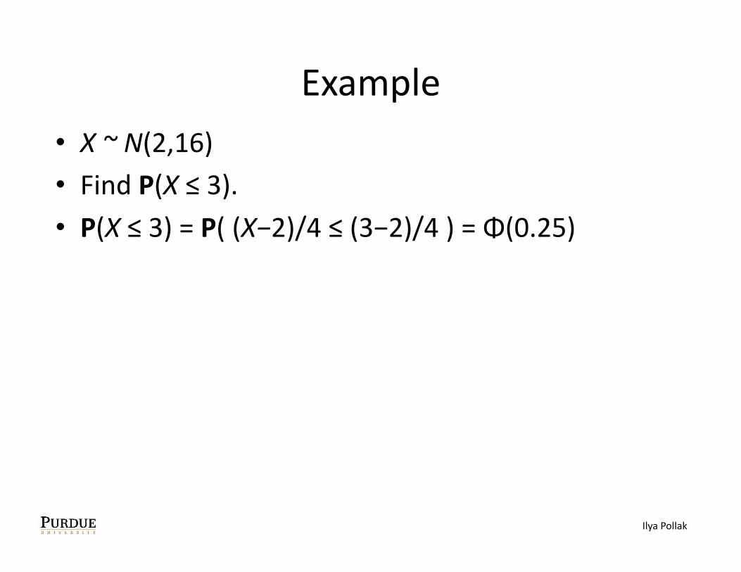
Example • X ~ N(2,16) • Find P(X ≤ 3). • P(X ≤ 3) = P( (X−2)/4 ≤ (3−2)/4 ) = Φ(0.25)
Ilya Pollak
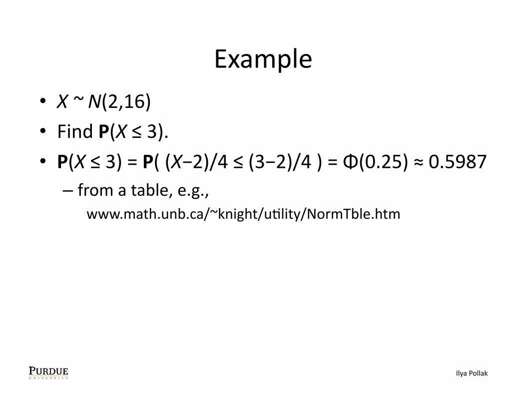
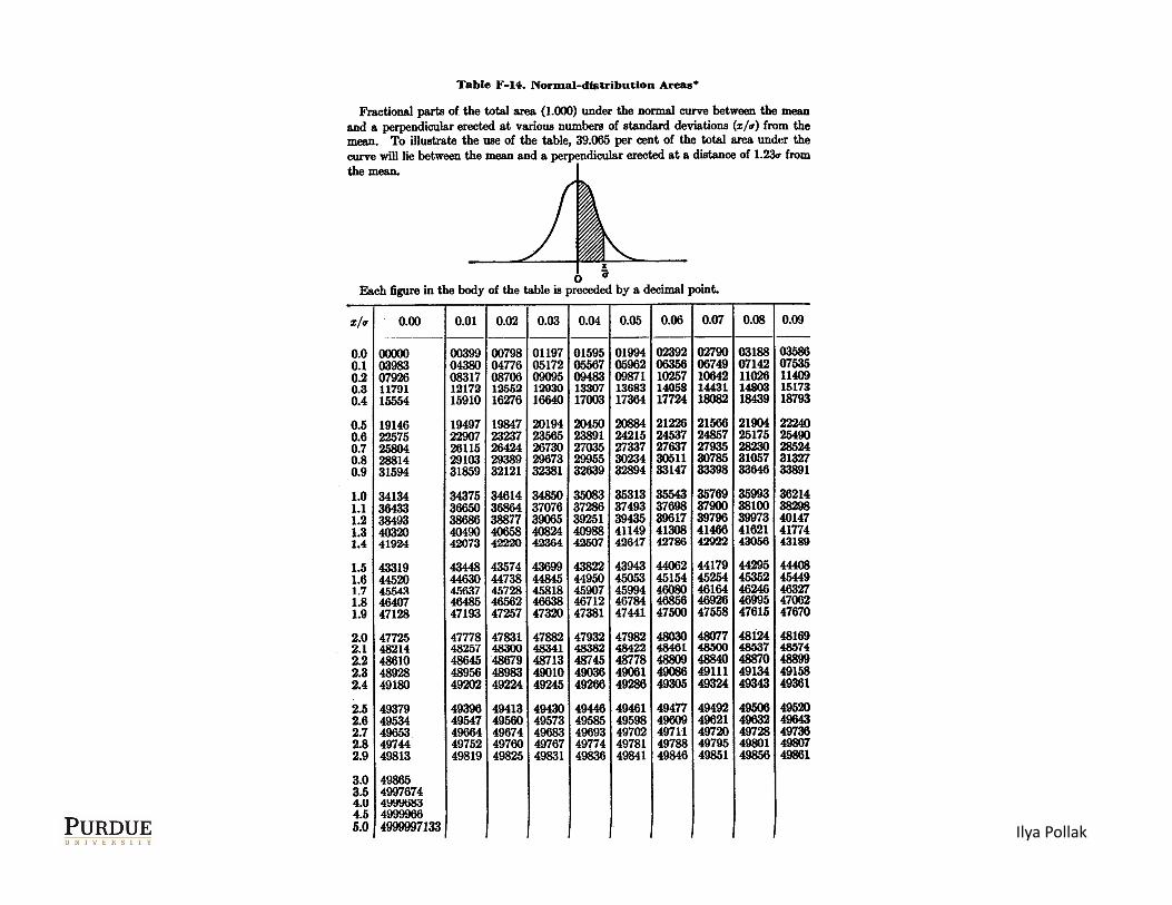
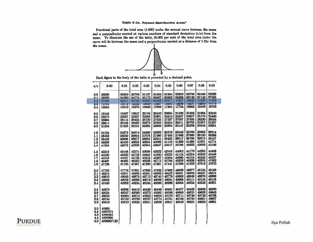
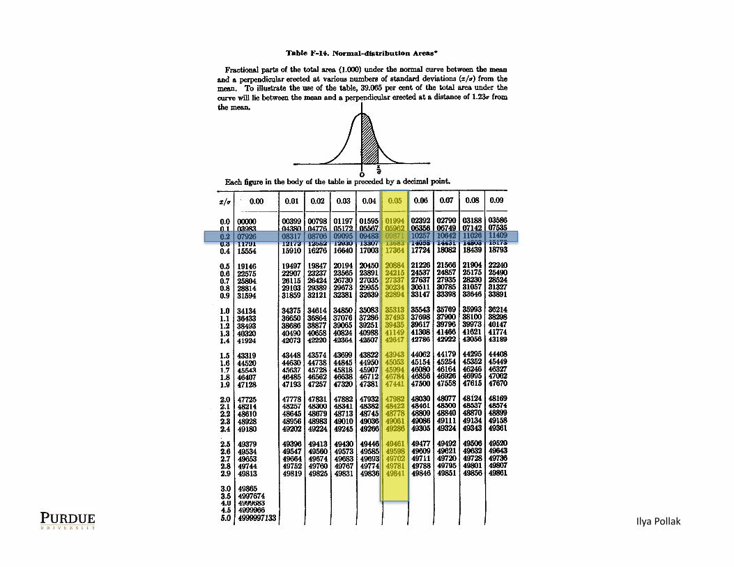
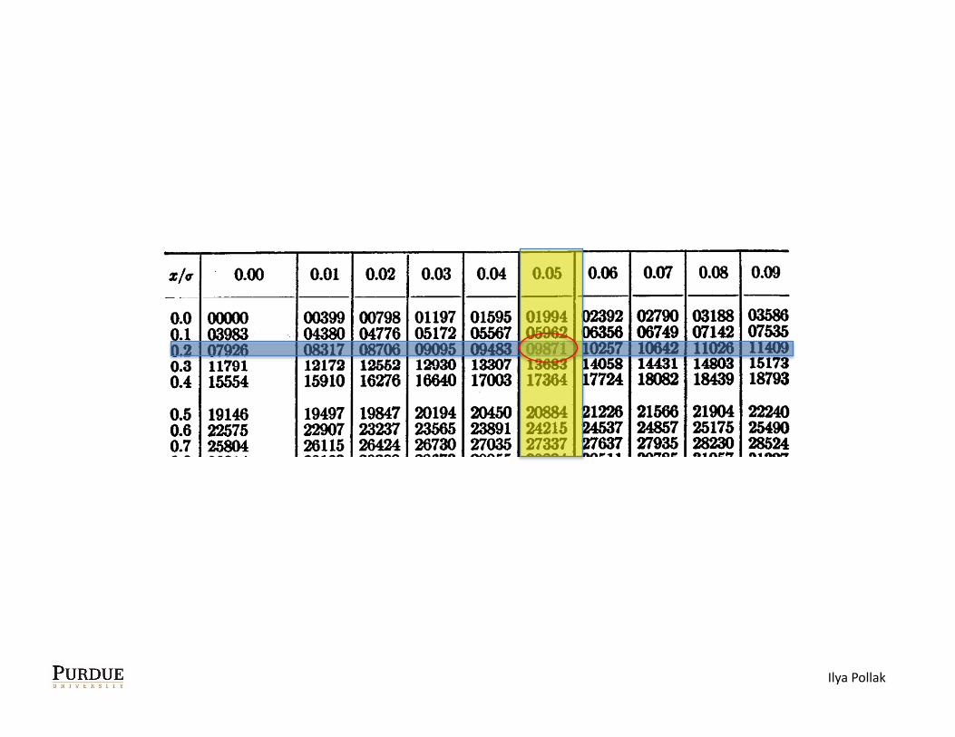
Example • X ~ N(2,16) • Find P(X ≤ 3). • P(X ≤ 3) = P( (X−2)/4 ≤ (3−2)/4 ) = Φ(0.25) ≈ 0.5987
– from a table, e.g., www.math.unb.ca/~knight/uKlity/NormTble.htm
Ilya Pollak
Ilya Pollak
Ilya Pollak
Ilya Pollak

Ilya Pollak
Ilya Pollak
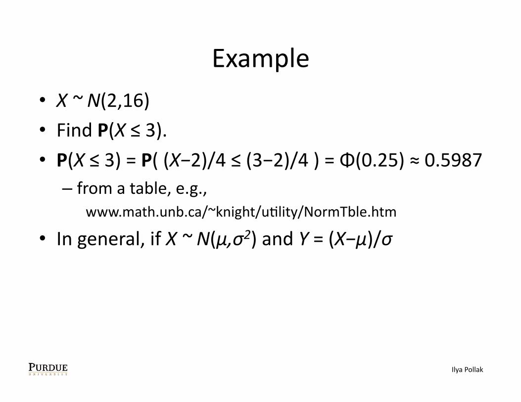
Example • X ~ N(2,16) • Find P(X ≤ 3). • P(X ≤ 3) = P( (X−2)/4 ≤ (3−2)/4 ) = Φ(0.25) ≈ 0.5987
– from a table, e.g., www.math.unb.ca/~knight/uKlity/NormTble.htm
• In general, if X ~ N(μ,σ2) and Y = (X−μ)/σ
Ilya Pollak
Example • X ~ N(2,16) • Find P(X ≤ 3). • P(X ≤ 3) = P( (X−2)/4 ≤ (3−2)/4 ) = Φ(0.25) ≈ 0.5987
– from a table, e.g., www.math.unb.ca/~knight/uKlity/NormTble.htm
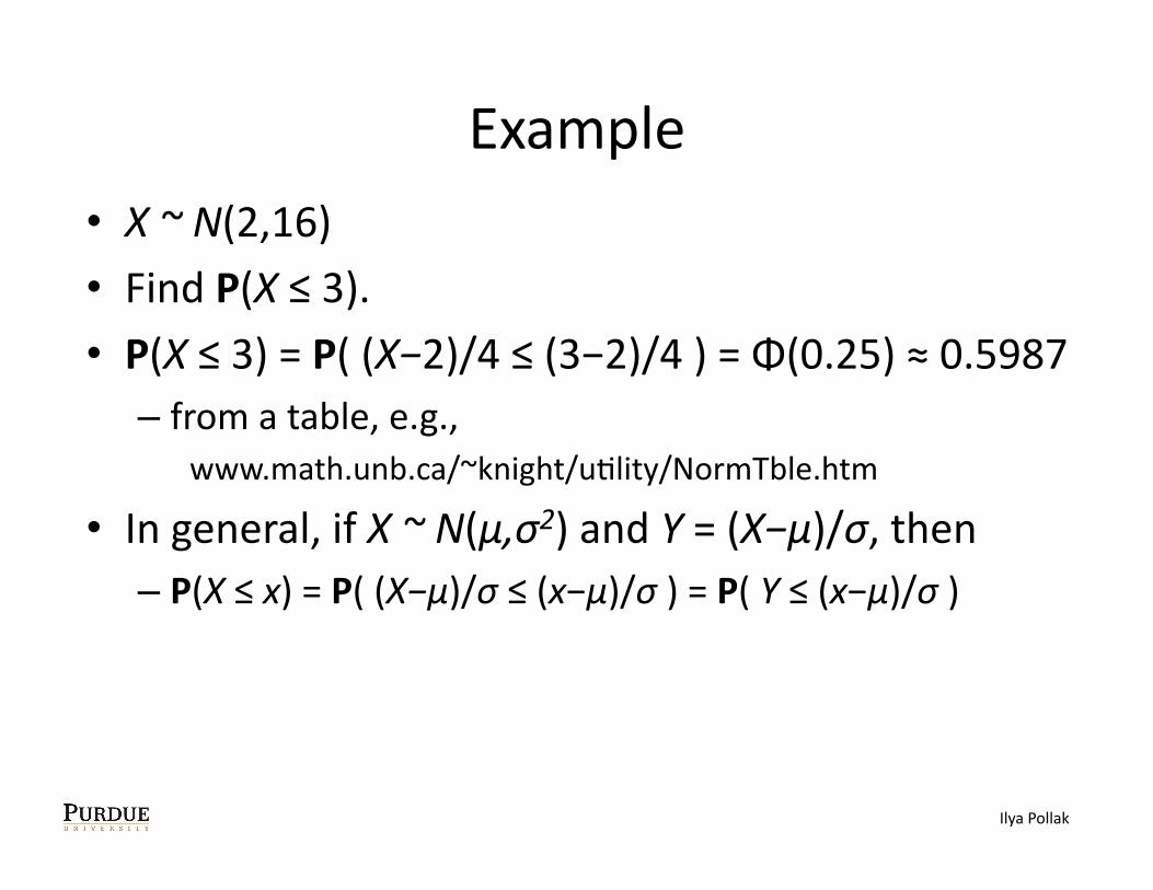
• In general, if X ~ N(μ,σ2) and Y = (X−μ)/σ, then – P(X ≤ x) = P( (X−μ)/σ ≤ (x−μ)/σ ) = P( Y ≤ (x−μ)/σ )
Ilya Pollak
Example • X ~ N(2,16) • Find P(X ≤ 3). • P(X ≤ 3) = P( (X−2)/4 ≤ (3−2)/4 ) = Φ(0.25) ≈ 0.5987
– from a table, e.g., www.math.unb.ca/~knight/uKlity/NormTble.htm
• In general, if X ~ N(μ,σ2) and Y = (X−μ)/σ, then – P(X ≤ x) = P( (X−μ)/σ ≤ (x−μ)/σ ) = P( Y ≤ (x−μ)/σ ) = Φ( (x−μ)/σ ),
– because Y ~ N(0,1)
Ilya Pollak
Then there is Wolfram Alpha
• cdf[normal distribuKon, mean 1, standard deviaKon 3, 2] computes the CDF of a N(1,9) random variable at 2.
Then there is Wolfram Alpha and other soiware packages
• cdf[normal distribuKon, mean 1, standard deviaKon 3, 2] computes the CDF of a N(1,9) random variable at 2.
• Most scienKfic soiware packages (e.g., Matlab) have normal CDF.
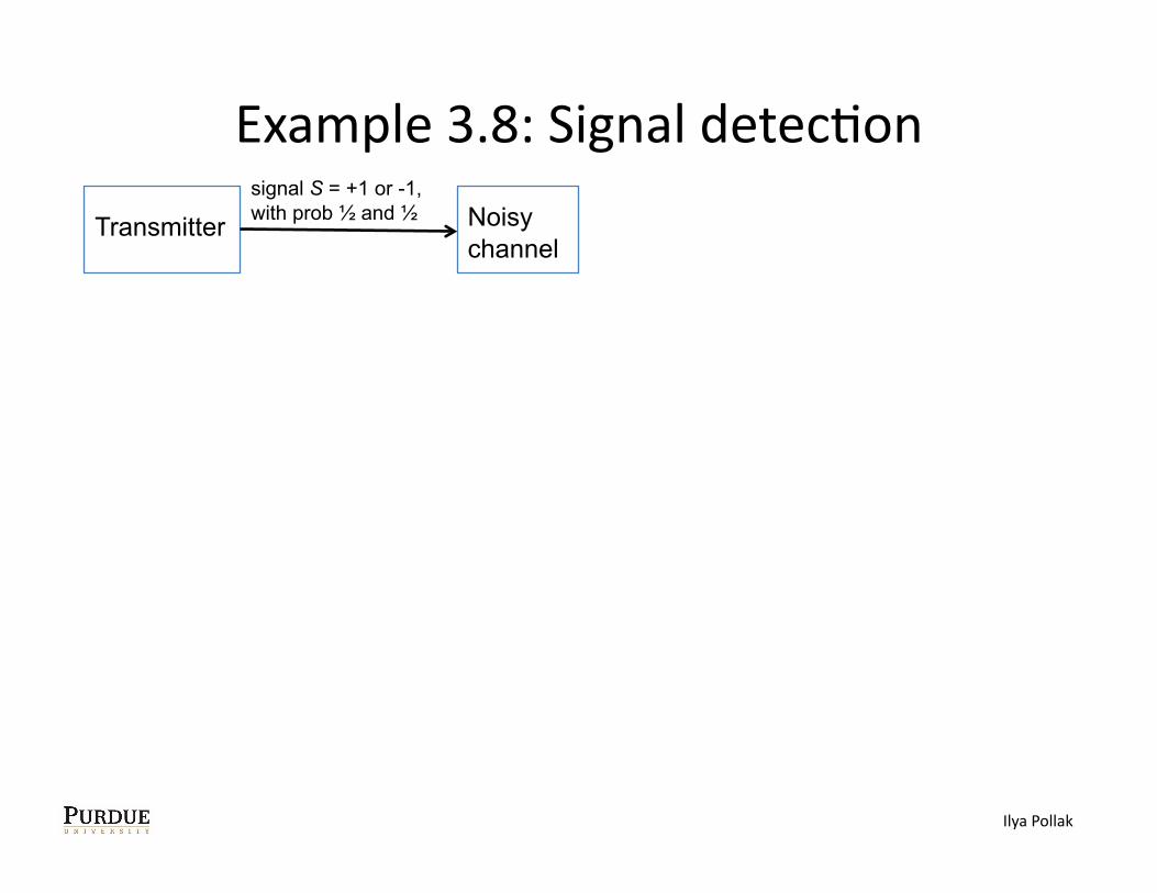
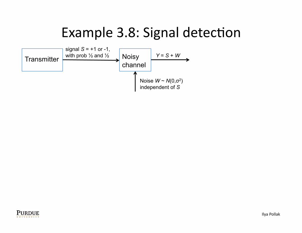
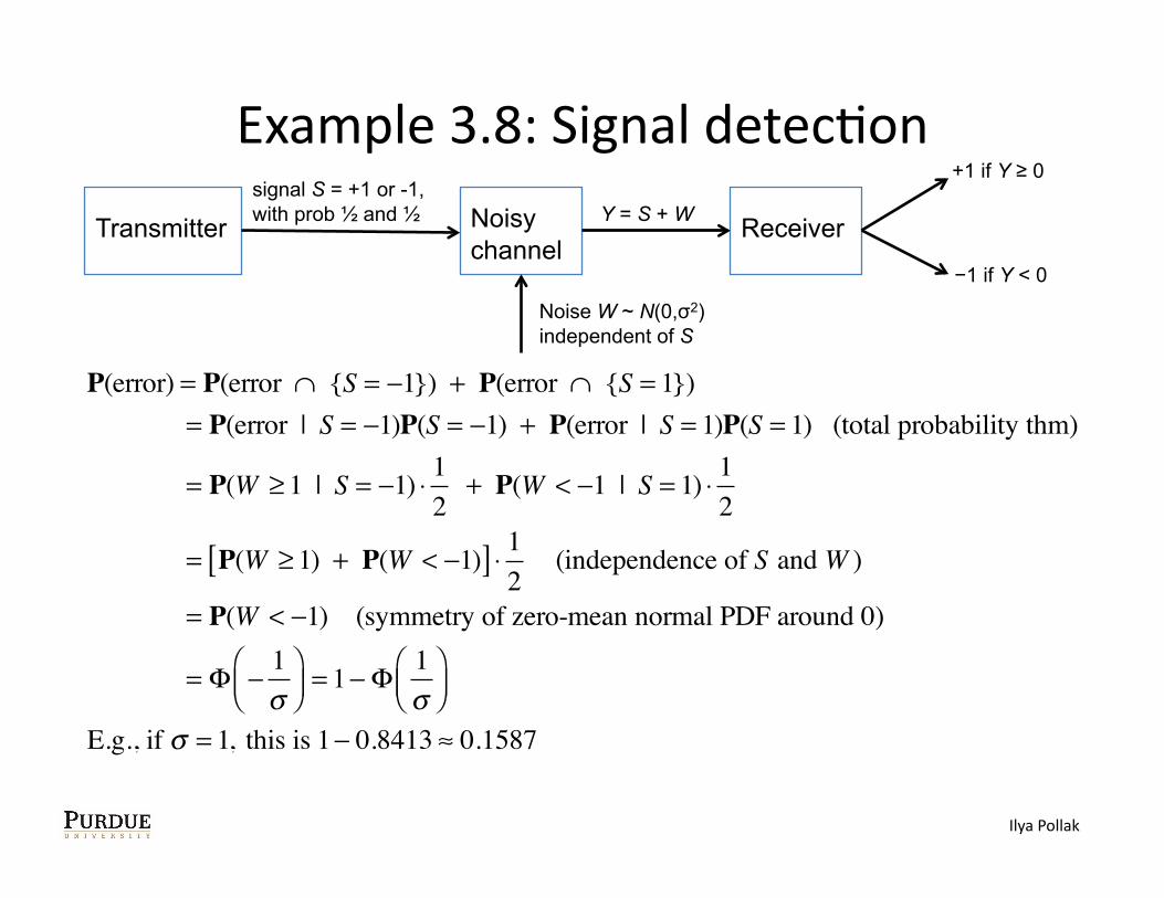
Example 3.8: Signal detecKon
Transmitter Noisy channel
signal S = +1 or -1, with prob ½ and ½
Ilya Pollak
Example 3.8: Signal detecKon
Transmitter Noisy channel
signal S = +1 or -1, with prob ½ and ½
Noise W ~ N(0,σ2) independent of S
Y = S + W
Ilya Pollak
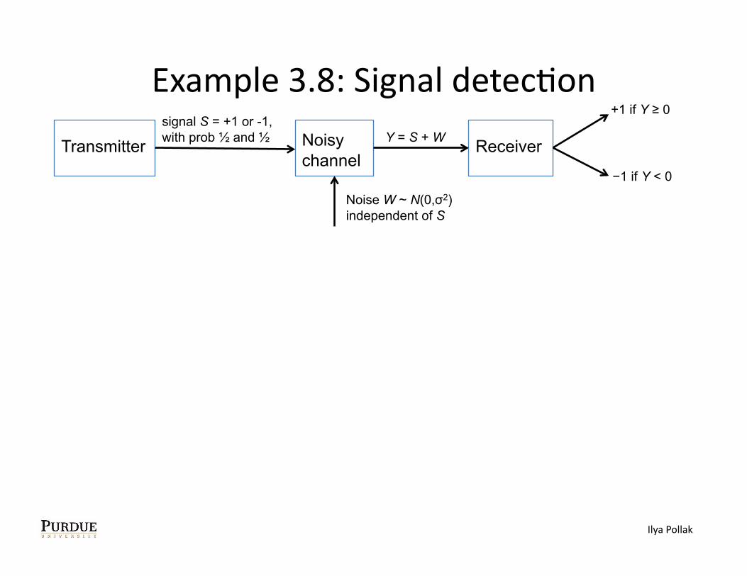
Example 3.8: Signal detecKon
Transmitter Noisy channel
Receiver signal S = +1 or -1, with prob ½ and ½
Noise W ~ N(0,σ2) independent of S
Y = S + W
+1 if Y ≥ 0
−1 if Y < 0
Ilya Pollak
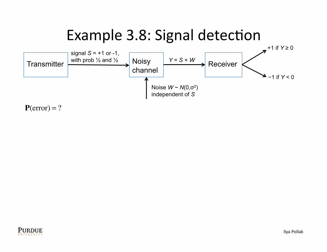
Example 3.8: Signal detecKon
Transmitter Noisy channel
Receiver signal S = +1 or -1, with prob ½ and ½
Noise W ~ N(0,σ2) independent of S
Y = S + W
+1 if Y ≥ 0
−1 if Y < 0
�
P(error) = ?
Ilya Pollak
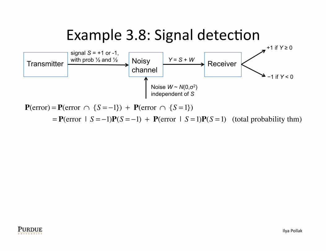
Example 3.8: Signal detecKon
Transmitter Noisy channel
Receiver signal S = +1 or -1, with prob ½ and ½
Noise W ~ N(0,σ2) independent of S
Y = S + W
+1 if Y ≥ 0
−1 if Y < 0
�
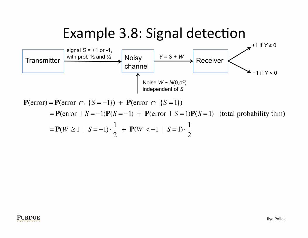
P(error) = P(error ∩ {S = −1}) + P(error ∩ {S = 1}) = P(error | S = −1)P(S = −1) + P(error | S = 1)P(S = 1) (total probability thm)
Ilya Pollak
Example 3.8: Signal detecKon
Transmitter Noisy channel
Receiver signal S = +1 or -1, with prob ½ and ½
Noise W ~ N(0,σ2) independent of S
Y = S + W
+1 if Y ≥ 0
−1 if Y < 0
�
P(error) = P(error ∩ {S = −1}) + P(error ∩ {S = 1}) = P(error | S = −1)P(S = −1) + P(error | S = 1)P(S = 1) (total probability thm)
= P(W ≥1 | S = −1) ⋅ 12
+ P(W < −1 | S = 1) ⋅ 12
Ilya Pollak
Example 3.8: Signal detecKon
Transmitter Noisy channel
Receiver signal S = +1 or -1, with prob ½ and ½
Noise W ~ N(0,σ2) independent of S
Y = S + W
+1 if Y ≥ 0
−1 if Y < 0
�
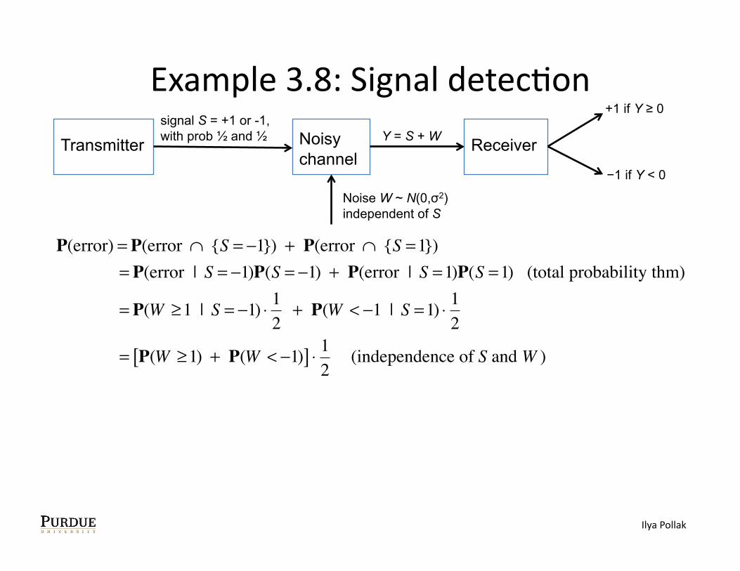
P(error) = P(error ∩ {S = −1}) + P(error ∩ {S = 1}) = P(error | S = −1)P(S = −1) + P(error | S = 1)P(S = 1) (total probability thm)
= P(W ≥1 | S = −1) ⋅ 12
+ P(W < −1 | S = 1) ⋅ 12
= P(W ≥1) + P(W < −1)[ ] ⋅ 12
(independence of S and W )
Ilya Pollak
Example 3.8: Signal detecKon
Transmitter Noisy channel
Receiver signal S = +1 or -1, with prob ½ and ½
Noise W ~ N(0,σ2) independent of S
Y = S + W
+1 if Y ≥ 0
−1 if Y < 0
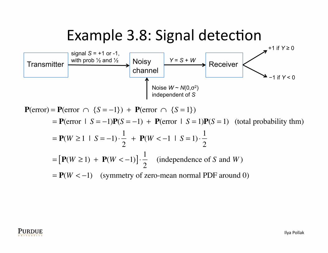
P(error) = P(error ∩ {S = −1}) + P(error ∩ {S = 1}) = P(error | S = −1)P(S = −1) + P(error | S = 1)P(S = 1) (total probability thm)
= P(W ≥ 1 | S = −1) ⋅ 12
+ P(W < −1 | S = 1) ⋅ 12
= P(W ≥ 1) + P(W < −1)[ ] ⋅ 12
(independence of S and W )
= P(W < −1) (symmetry of zero-mean normal PDF around 0)
Ilya Pollak
Example 3.8: Signal detecKon
Transmitter Noisy channel
Receiver signal S = +1 or -1, with prob ½ and ½
Noise W ~ N(0,σ2) independent of S
Y = S + W
+1 if Y ≥ 0
−1 if Y < 0
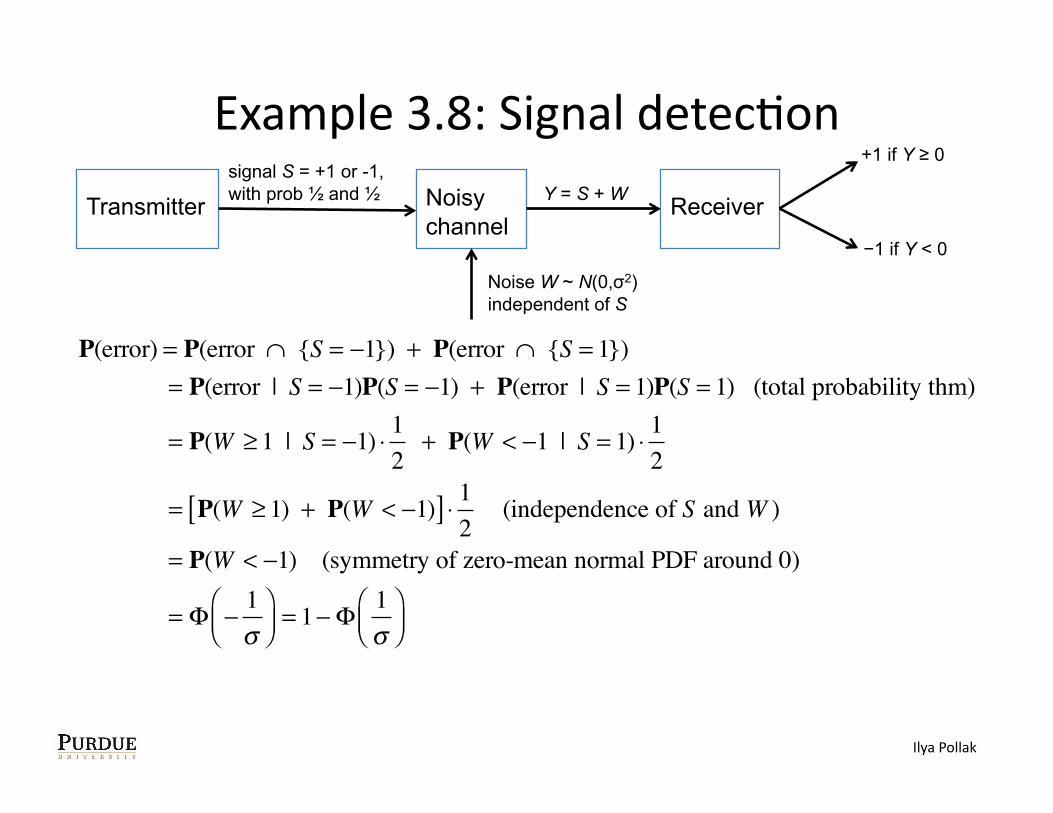
P(error) = P(error ∩ {S = −1}) + P(error ∩ {S = 1}) = P(error | S = −1)P(S = −1) + P(error | S = 1)P(S = 1) (total probability thm)
= P(W ≥ 1 | S = −1) ⋅ 12
+ P(W < −1 | S = 1) ⋅ 12
= P(W ≥ 1) + P(W < −1)[ ] ⋅ 12
(independence of S and W )
= P(W < −1) (symmetry of zero-mean normal PDF around 0)
= Φ −1σ
⎛⎝⎜
⎞⎠⎟= 1− Φ
1σ
⎛⎝⎜
⎞⎠⎟
Ilya Pollak
Example 3.8: Signal detecKon
Transmitter Noisy channel
Receiver signal S = +1 or -1, with prob ½ and ½
Noise W ~ N(0,σ2) independent of S
Y = S + W
+1 if Y ≥ 0
−1 if Y < 0
P(error) = P(error ∩ {S = −1}) + P(error ∩ {S = 1}) = P(error | S = −1)P(S = −1) + P(error | S = 1)P(S = 1) (total probability thm)
= P(W ≥ 1 | S = −1) ⋅ 12
+ P(W < −1 | S = 1) ⋅ 12
= P(W ≥ 1) + P(W < −1)[ ] ⋅ 12
(independence of S and W )
= P(W < −1) (symmetry of zero-mean normal PDF around 0)
= Φ −1σ
⎛⎝⎜
⎞⎠⎟= 1− Φ
1σ
⎛⎝⎜
⎞⎠⎟
E.g., if σ = 1, this is 1− 0.8413 ≈ 0.1587
Ilya Pollak
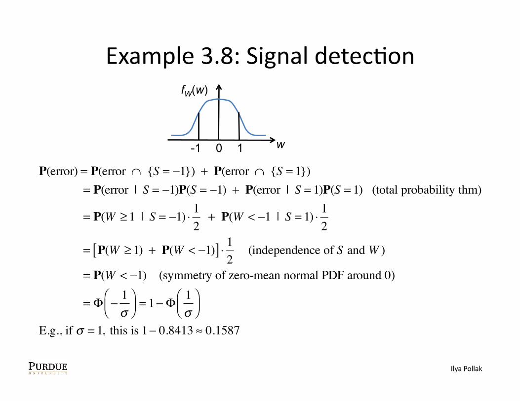
Example 3.8: Signal detecKon
P(error) = P(error ∩ {S = −1}) + P(error ∩ {S = 1}) = P(error | S = −1)P(S = −1) + P(error | S = 1)P(S = 1) (total probability thm)
= P(W ≥ 1 | S = −1) ⋅ 12
+ P(W < −1 | S = 1) ⋅ 12
= P(W ≥ 1) + P(W < −1)[ ] ⋅ 12
(independence of S and W )
= P(W < −1) (symmetry of zero-mean normal PDF around 0)
= Φ −1σ
⎛⎝⎜
⎞⎠⎟= 1− Φ
1σ
⎛⎝⎜
⎞⎠⎟
E.g., if σ = 1, this is 1− 0.8413 ≈ 0.1587
fW(w)
0 w -1 1
Ilya Pollak
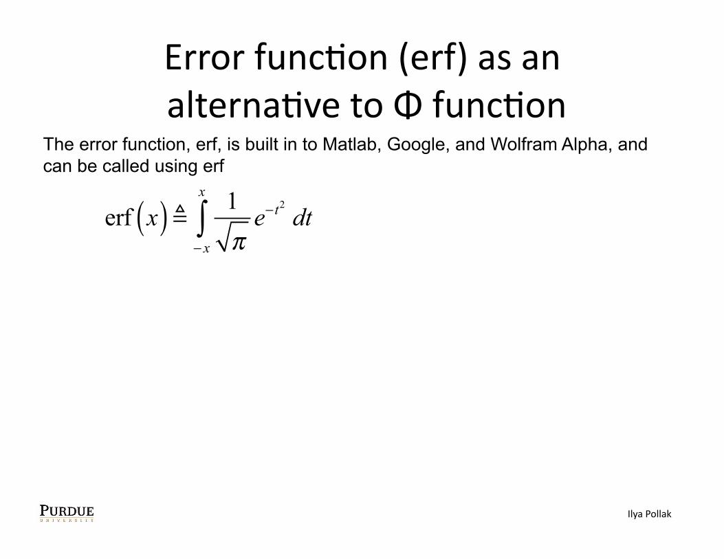
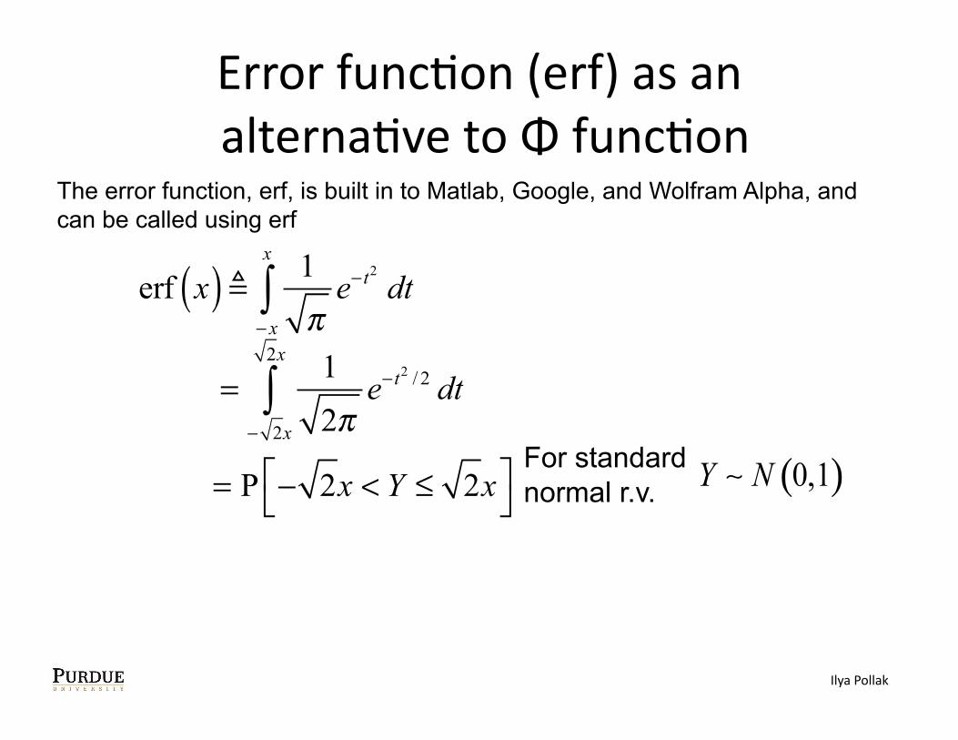
Error funcKon (erf) as an alternaKve to Φ funcKon
erf x( ) 1πe− t
2
dt− x
x
∫
The error function, erf, is built in to Matlab, Google, and Wolfram Alpha, and can be called using erf
Ilya Pollak
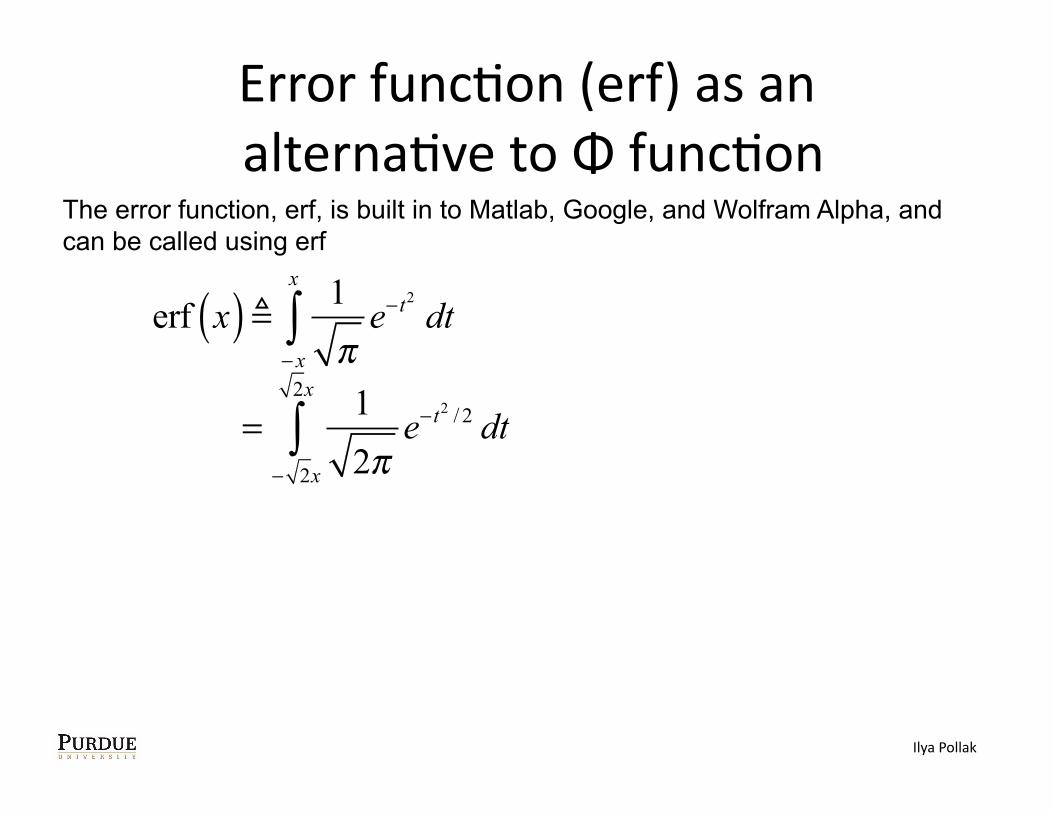
Error funcKon (erf) as an alternaKve to Φ funcKon
erf x( ) 1πe− t
2
dt− x
x
∫
=12πe− t
2 / 2 dt− 2x
2x
∫
Ilya Pollak
The error function, erf, is built in to Matlab, Google, and Wolfram Alpha, and can be called using erf
Error funcKon (erf) as an alternaKve to Φ funcKon
erf x( ) 1πe− t
2
dt− x
x
∫
=12πe− t
2 / 2 dt− 2x
2x
∫
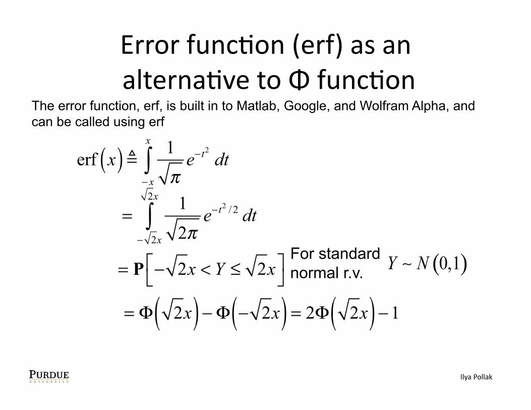
= P − 2x < Y ≤ 2x⎡⎣
⎤⎦
For standard normal r.v.
Ilya Pollak
The error function, erf, is built in to Matlab, Google, and Wolfram Alpha, and can be called using erf
Error funcKon (erf) as an alternaKve to Φ funcKon
erf x( ) 1πe− t
2
dt− x
x
∫
=12πe− t
2 / 2 dt− 2x
2x
∫
= P − 2x < Y ≤ 2x⎡⎣
⎤⎦
For standard normal r.v.
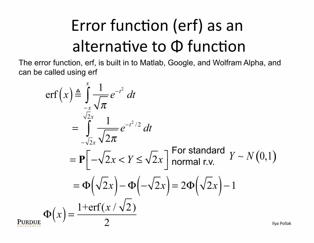
= Φ 2x( ) − Φ − 2x( ) = 2Φ 2x( ) −1Ilya Pollak
The error function, erf, is built in to Matlab, Google, and Wolfram Alpha, and can be called using erf
Error funcKon (erf) as an alternaKve to Φ funcKon
erf x( ) 1πe− t
2
dt− x
x
∫
=12πe− t
2 / 2 dt− 2x
2x
∫
= P − 2x < Y ≤ 2x⎡⎣
⎤⎦
For standard normal r.v.
= Φ 2x( ) − Φ − 2x( ) = 2Φ 2x( ) −1Φ x( ) = 1+erf (x / 2)
2 Ilya Pollak
The error function, erf, is built in to Matlab, Google, and Wolfram Alpha, and can be called using erf


![18/3/2015 [Συζήτηση για την Ανθρωπιστική Κρίση]](https://static.fdocument.org/doc/165x107/55cf916c550346f57b8d6de3/1832015-.jpg)