RA15 C2 intferometry concepts v1 Astronomy, Leiden, 13 Feb 2015 /01 Nature of radiation •Radio...
36
Interferometry Concepts Huib Jan van Langevelde JIVE /Leiden
-
Upload
nguyendiep -
Category
Documents
-
view
215 -
download
2
Transcript of RA15 C2 intferometry concepts v1 Astronomy, Leiden, 13 Feb 2015 /01 Nature of radiation •Radio...
Interferometry Concepts
Huib Jan van Langevelde
JIVE/Leiden
hu
ib 1
1/0
2/1
5
/33Radio Astronomy, Leiden, 13 Feb 2015
Hello
!
•Introduction
!
•Do we all know our Fourier transforms?
!
•Done your homework?
2
hu
ib 1
1/0
2/1
5
/33Radio Astronomy, Leiden, 13 Feb 2015
Practical work
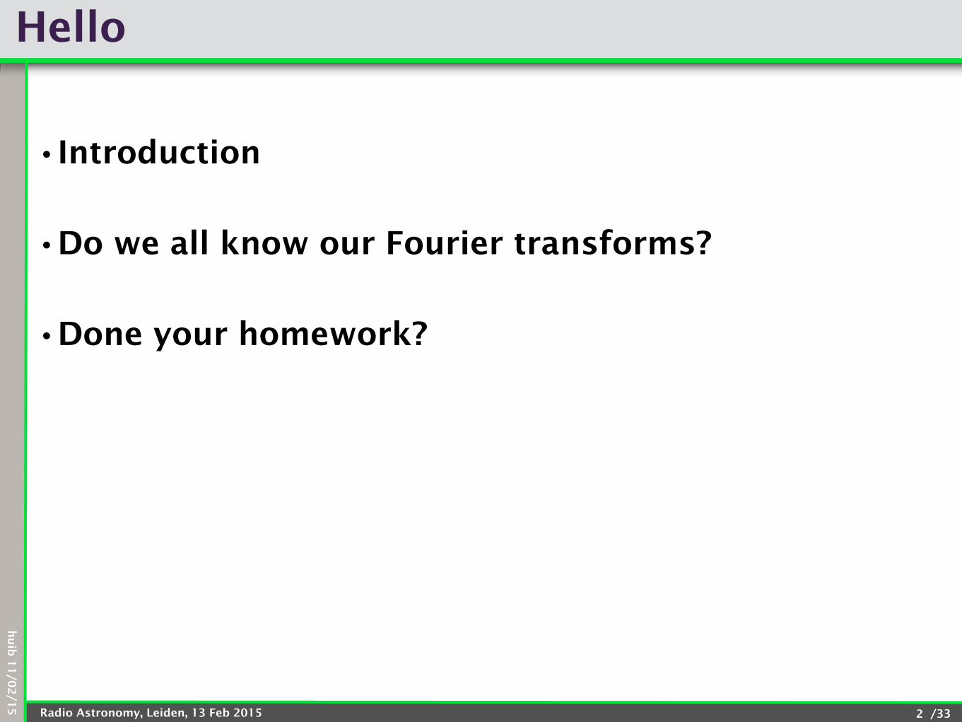
•Tutorials •Objective basic concepts interferometry
•And introduction to casa, get ready for Assignments
•Two sessions: 13 and 20 February •13 March will take all afternoon in HL411 (13:45 - 17:30)
•20 March will follow normal lecture HL414 - HL411 (15:45 - 17:30)
•Assignments •Objective: research a data processing problem independently
•HL411 + assistance available every week
•Form: write a short report (max 3000 words) with scientific discussion •Preferably done in pairs, could be singles (but no groups of 3)
•Choose somebody with similar experience
•Pick one of 3 assignments based on experience (will coordinate this on 27 Feb)
•Evaluation: will form 25% of your mark •Must be turned in May 8, well before oral exam
•Report will be discussed at the exam and grade determined there
3
https://www.astron.nl/~mag/dokuwiki/doku.php?id=radio_astronomy_course_description:practicum
hu
ib 1
1/0
2/1
5
/33Radio Astronomy, Leiden, 13 Feb 2015
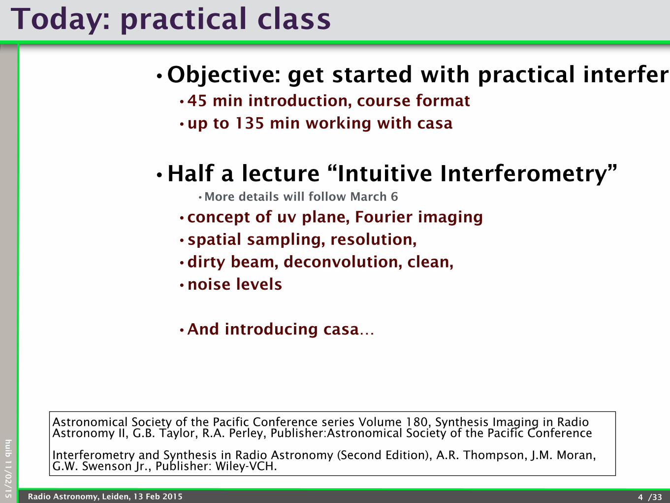
Today: practical class
•Objective: get started with practical interferometry •45 min introduction, course format
•up to 135 min working with casa
!
•Half a lecture “Intuitive Interferometry” •More details will follow March 6
•concept of uv plane, Fourier imaging
•spatial sampling, resolution,
•dirty beam, deconvolution, clean,
•noise levels
!•And introducing casa…
4
Astronomical Society of the Pacific Conference series Volume 180, Synthesis Imaging in Radio Astronomy II, G.B. Taylor, R.A. Perley, Publisher:Astronomical Society of the Pacific Conference !Interferometry and Synthesis in Radio Astronomy (Second Edition), A.R. Thompson, J.M. Moran, G.W. Swenson Jr., Publisher: Wiley-VCH.
/01Radio Astronomy, Leiden, 13 Feb 2015
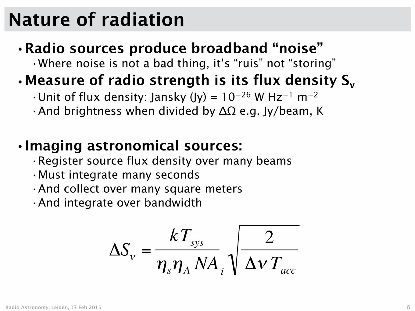
Nature of radiation
•Radio sources produce broadband “noise” •Where noise is not a bad thing, it’s “ruis” not “storing”
•Measure of radio strength is its flux density Sν
•Unit of flux density: Jansky (Jy) = 10−26 W Hz−1 m−2
•And brightness when divided by ΔΩ e.g. Jy/beam, K
!•Imaging astronomical sources:
•Register source flux density over many beams •Must integrate many seconds •And collect over many square meters •And integrate over bandwidth
5
€
ΔSν =kTsys
ηsηA NA i
2Δν Tacc
!
/01Radio Astronomy, Leiden, 13 Feb 2015
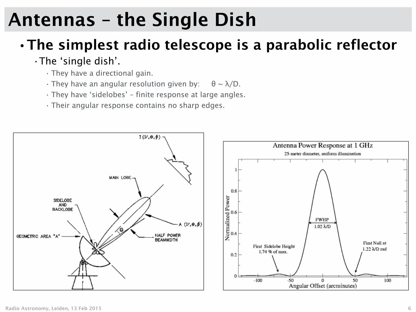
Antennas – the Single Dish•The simplest radio telescope is a parabolic reflector
•The ‘single dish’. • They have a directional gain.
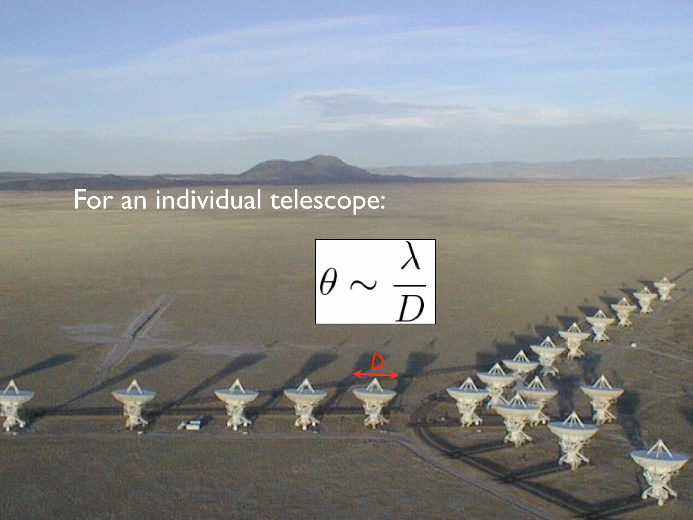
• They have an angular resolution given by: θ ~ λ/D.
• They have ‘sidelobes’ – finite response at large angles.
• Their angular response contains no sharp edges.
6
/01Radio Astronomy, Leiden, 13 Feb 2015
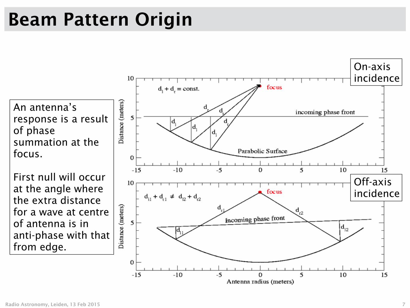
Beam Pattern Origin
7
An antenna’s response is a result of phase summation at the focus. !First null will occur at the angle where the extra distance for a wave at centre of antenna is in anti-phase with that from edge.
On-axis incidence
Off-axis incidence
/01Radio Astronomy, Leiden, 13 Feb 2015
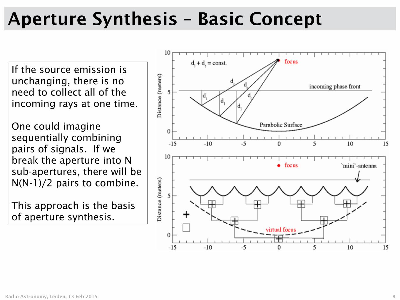
Aperture Synthesis – Basic Concept
8
If the source emission is unchanging, there is no need to collect all of the incoming rays at one time. !One could imagine sequentially combining pairs of signals. If we break the aperture into N sub-apertures, there will be N(N-1)/2 pairs to combine. !This approach is the basis of aperture synthesis.
/01Radio Astronomy, Leiden, 13 Feb 2015 9
D
For an individual telescope:
/01Radio Astronomy, Leiden, 13 Feb 2015 10
B
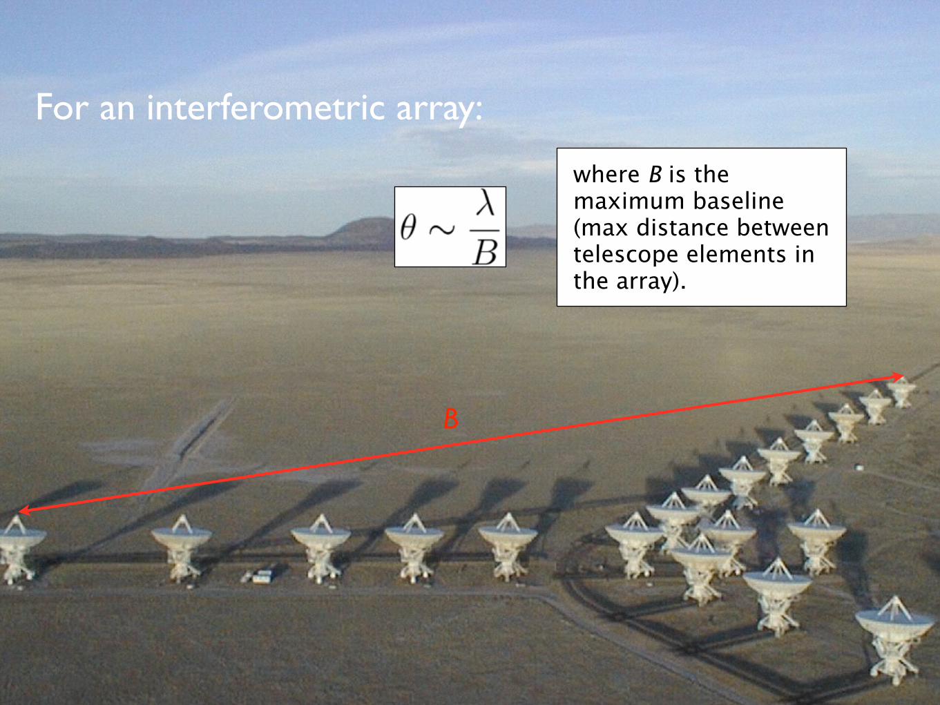
where B is the maximum baseline (max distance between telescope elements in the array).
For an interferometric array:
/01Radio Astronomy, Leiden, 13 Feb 2015 11
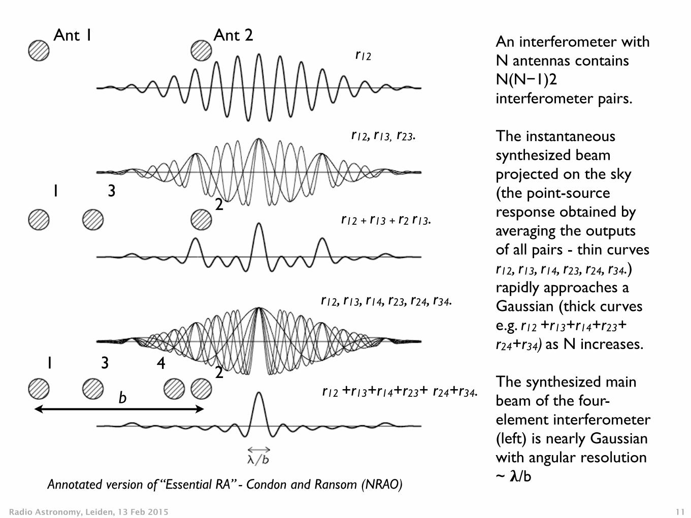
An interferometer with N antennas contains N(N−1)2 interferometer pairs. !The instantaneous synthesized beam projected on the sky (the point-source response obtained by averaging the outputs of all pairs - thin curves r12, r13, r14, r23, r24, r34.) rapidly approaches a Gaussian (thick curves e.g. r12 +r13+r14+r23+ r24+r34) as N increases. !The synthesized main beam of the four-element interferometer (left) is nearly Gaussian with angular resolution ~ 𝛌/b
r12
r12 + r13 + r2 r13.
r12, r13, r23.
r12, r13, r14, r23, r24, r34.
r12 +r13+r14+r23+ r24+r34.
Annotated version of “Essential RA” - Condon and Ransom (NRAO)
Ant 1 Ant 2
1
1
2
2
3
3 4
b
/01Radio Astronomy, Leiden, 13 Feb 2015
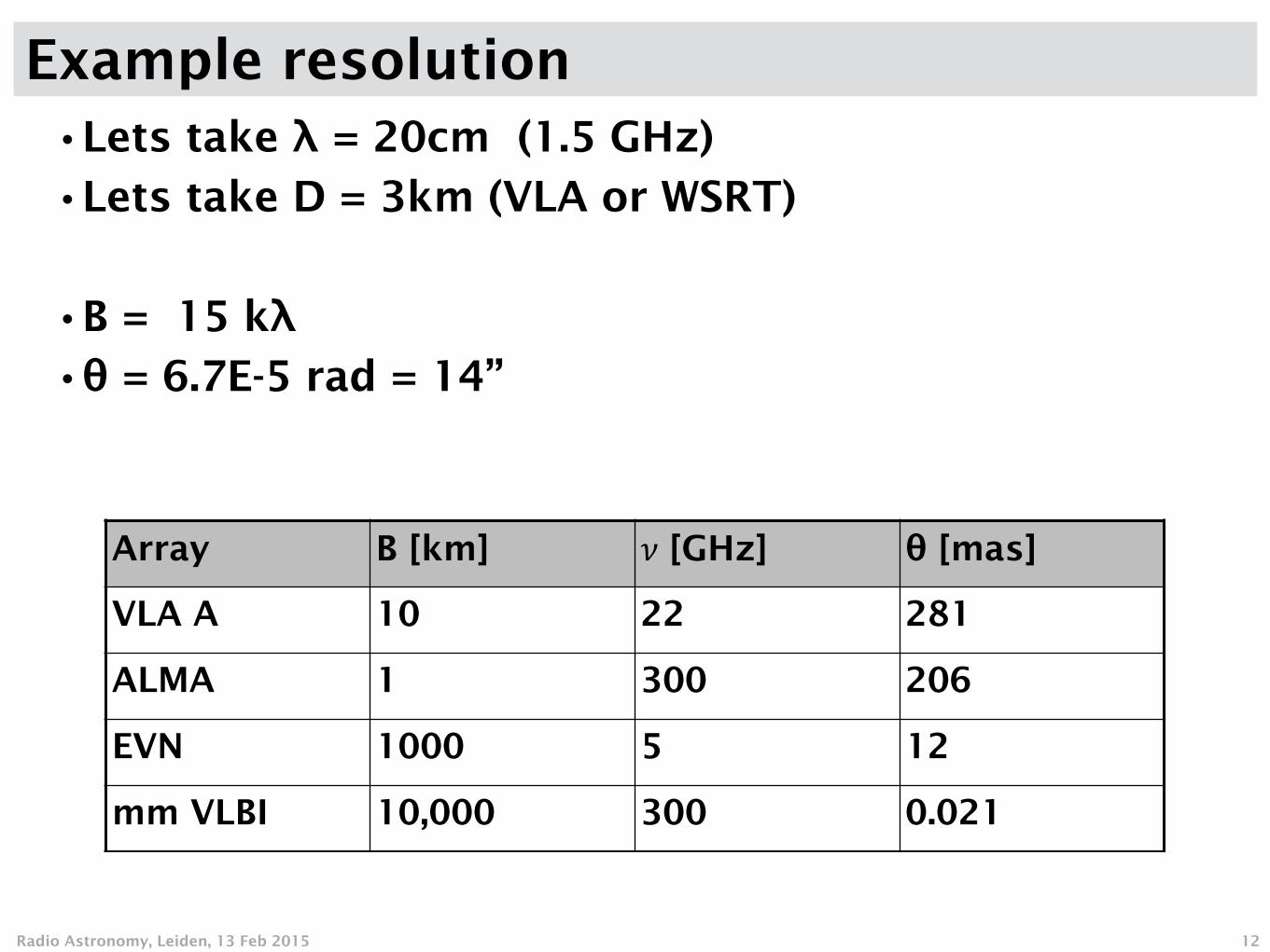
Example resolution•Lets take λ = 20cm (1.5 GHz)
•Lets take D = 3km (VLA or WSRT)
!
•B = 15 kλ
•θ = 6.7E-5 rad = 14”
12
Array B [km] 𝜈 [GHz] θ [mas]
VLA A 10 22 281
ALMA 1 300 206
EVN 1000 5 12
mm VLBI 10,000 300 0.021
/01Radio Astronomy, Leiden, 13 Feb 2015
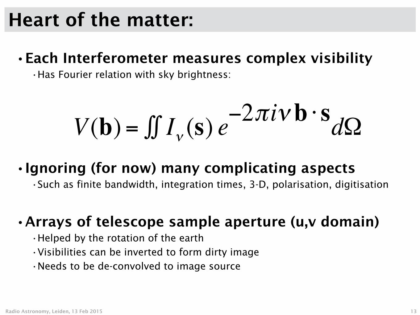
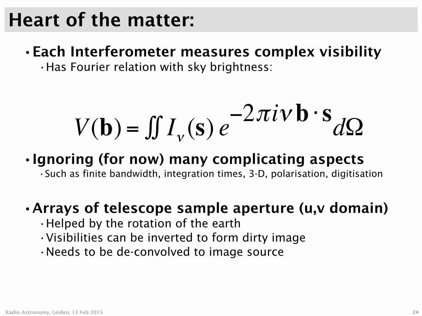
Heart of the matter:
•Each Interferometer measures complex visibility •Has Fourier relation with sky brightness:
!!!!
!
•Ignoring (for now) many complicating aspects •Such as finite bandwidth, integration times, 3-D, polarisation, digitisation
!
•Arrays of telescope sample aperture (u,v domain) •Helped by the rotation of the earth
•Visibilities can be inverted to form dirty image
•Needs to be de-convolved to image source
13
!
€
V (b) = Iν (s)∫∫ e−2π iν b ⋅ sdΩ
/01Radio Astronomy, Leiden, 13 Feb 2015
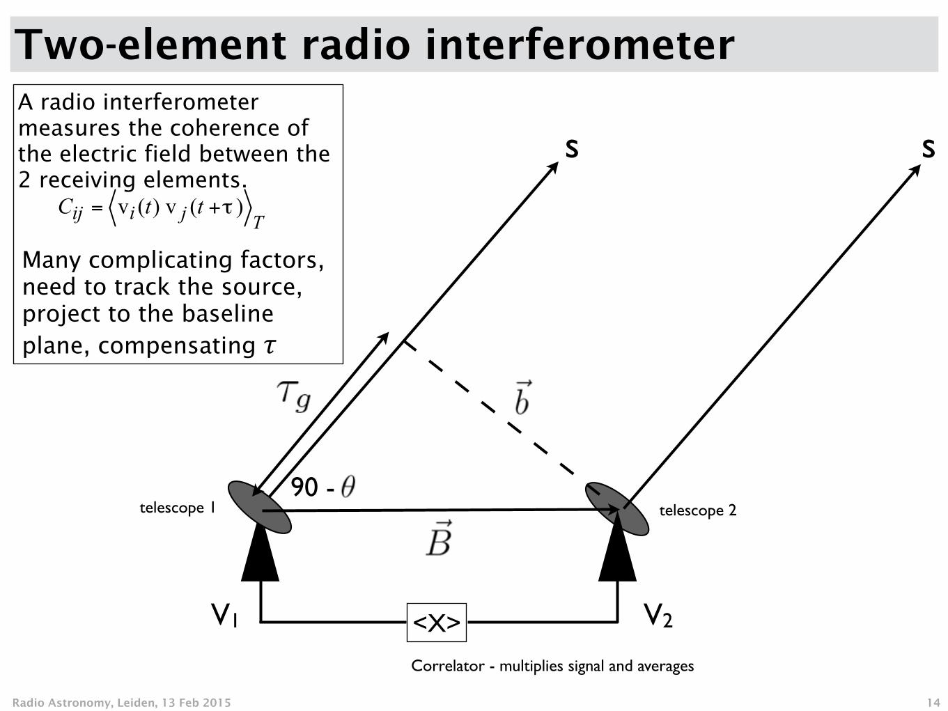
Two-element radio interferometer
14
<X>
Correlator - multiplies signal and averages
telescope 2telescope 1
s s
V1 V2
90 -
A radio interferometer measures the coherence of the electric field between the 2 receiving elements. !!Many complicating factors, need to track the source, project to the baseline plane, compensating 𝜏
Tjiij ttC )(v)(v τ+=

/01Radio Astronomy, Leiden, 13 Feb 2015
•Each Interferometer measures complex visibility •Has Fourier relation with sky brightness: !!!!
!•Ignoring (for now) many complicating aspects
•Such as finite bandwidth, integration times, 3-D, polarisation, digitisation
!•Arrays of telescope sample aperture (u,v domain)
•Helped by the rotation of the earth •Visibilities can be inverted to form dirty image •Needs to be de-convolved to image source
Heart of the matter:
15
!
€
V (b) = Iν (s)∫∫ e−2π iν b ⋅ sdΩ
/01Radio Astronomy, Leiden, 13 Feb 2015 16
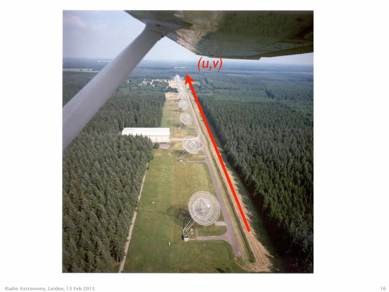
(u,v)
/01Radio Astronomy, Leiden, 13 Feb 2015 17
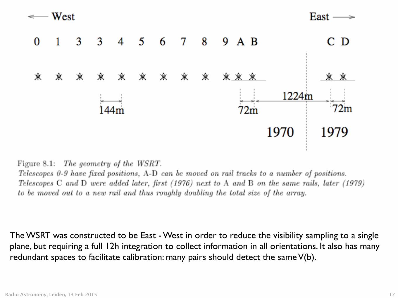
Westerbork telescope on rails.
The WSRT was constructed to be East - West in order to reduce the visibility sampling to a single plane, but requiring a full 12h integration to collect information in all orientations. It also has many redundant spaces to facilitate calibration: many pairs should detect the same V(b).
/01Radio Astronomy, Leiden, 13 Feb 2015 18
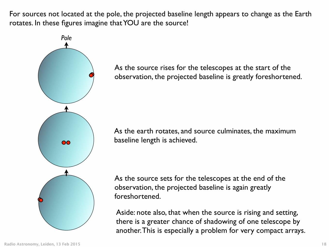
For sources not located at the pole, the projected baseline length appears to change as the Earth rotates. In these figures imagine that YOU are the source!
Pole
As the source rises for the telescopes at the start of the observation, the projected baseline is greatly foreshortened.
As the earth rotates, and source culminates, the maximum baseline length is achieved.
As the source sets for the telescopes at the end of the observation, the projected baseline is again greatly foreshortened.
Aside: note also, that when the source is rising and setting, there is a greater chance of shadowing of one telescope by another. This is especially a problem for very compact arrays.
/01Radio Astronomy, Leiden, 13 Feb 2015
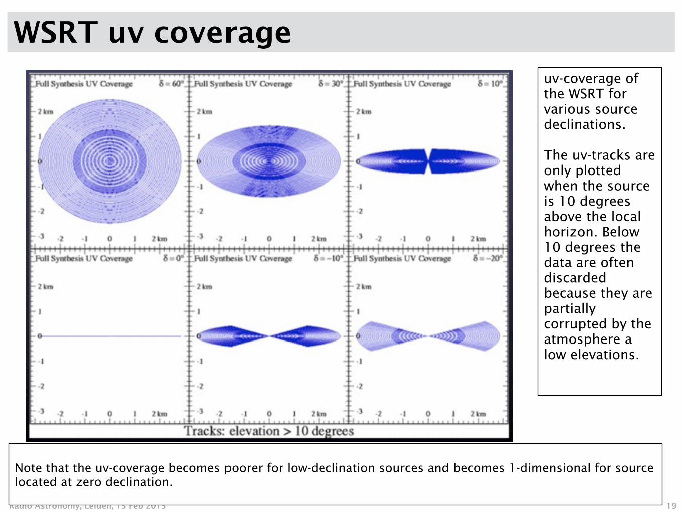
WSRT uv coverage
19
uv-coverage of the WSRT for various source declinations. !The uv-tracks are only plotted when the source is 10 degrees above the local horizon. Below 10 degrees the data are often discarded because they are partially corrupted by the atmosphere a low elevations. !
Note that the uv-coverage becomes poorer for low-declination sources and becomes 1-dimensional for source located at zero declination.

/01Radio Astronomy, Leiden, 13 Feb 2015
•Each Interferometer measures complex visibility •Has Fourier relation with sky brightness: !!!!
!•Ignoring (for now) many complicating aspects
•Such as finite bandwidth, integration times, 3-D, polarisation, digitisation
!•Arrays of telescope sample aperture (u,v domain)
•Helped by the rotation of the earth •Visibilities can be inverted to form dirty image •Needs to be de-convolved to image source
Heart of the matter:
20
!
€
V (b) = Iν (s)∫∫ e−2π iν b ⋅ sdΩ

/01Radio Astronomy, Leiden, 13 Feb 2015
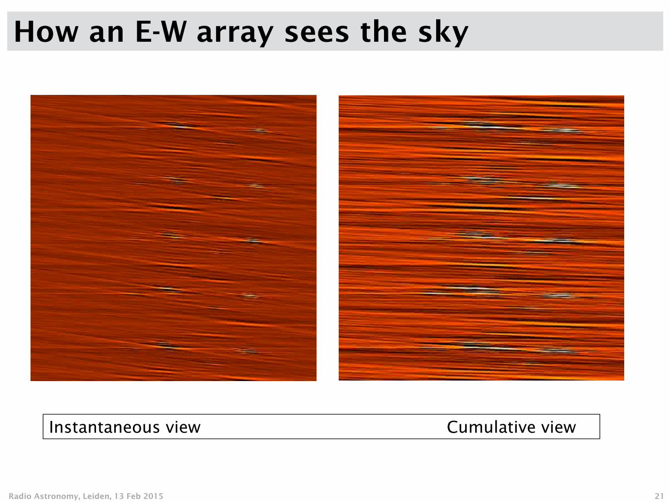
How an E-W array sees the sky
21
Instantaneous view Cumulative view
/01Radio Astronomy, Leiden, 13 Feb 2015
How an E-W array sees the sky
21
Instantaneous view Cumulative view
/01Radio Astronomy, Leiden, 13 Feb 2015
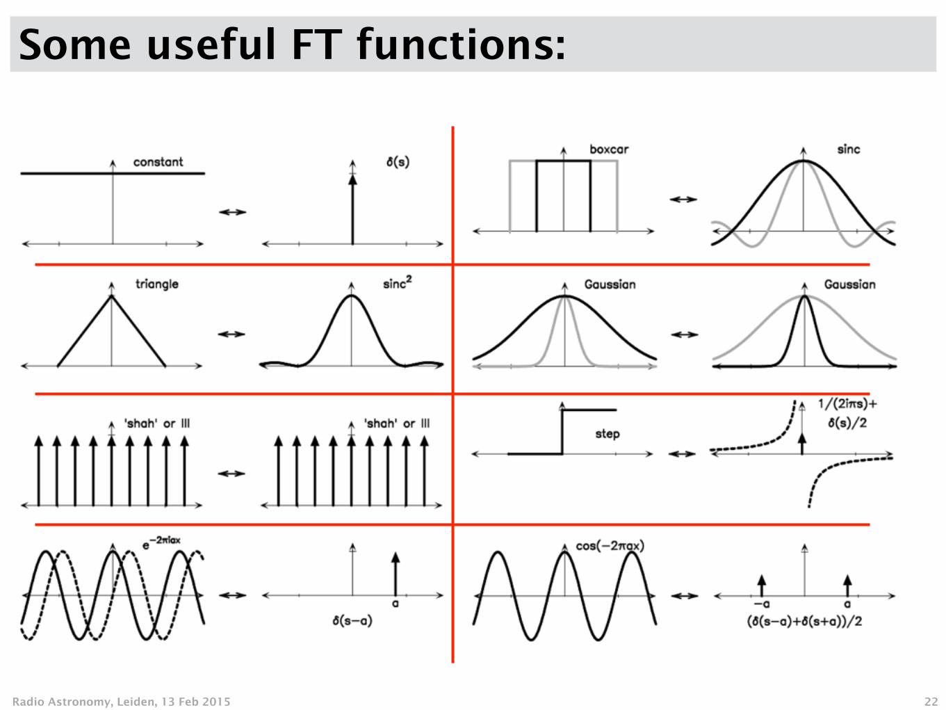
Some useful FT functions:
22
/01Radio Astronomy, Leiden, 13 Feb 2015
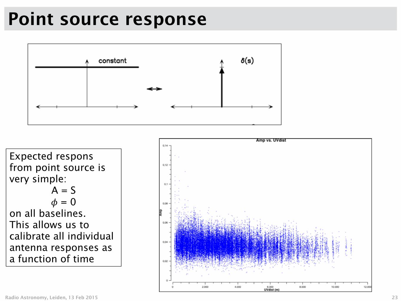
Point source response
23
Expected respons from point source is very simple:
A = S 𝜙 = 0
on all baselines. This allows us to calibrate all individual antenna responses as a function of time
/01Radio Astronomy, Leiden, 13 Feb 2015
•Each Interferometer measures complex visibility •Has Fourier relation with sky brightness: !!!!
!•Ignoring (for now) many complicating aspects
•Such as finite bandwidth, integration times, 3-D, polarisation, digitisation
!•Arrays of telescope sample aperture (u,v domain)
•Helped by the rotation of the earth •Visibilities can be inverted to form dirty image •Needs to be de-convolved to image source
Heart of the matter:
24
!
€
V (b) = Iν (s)∫∫ e−2π iν b ⋅ sdΩ
/01Radio Astronomy, Leiden, 13 Feb 2015
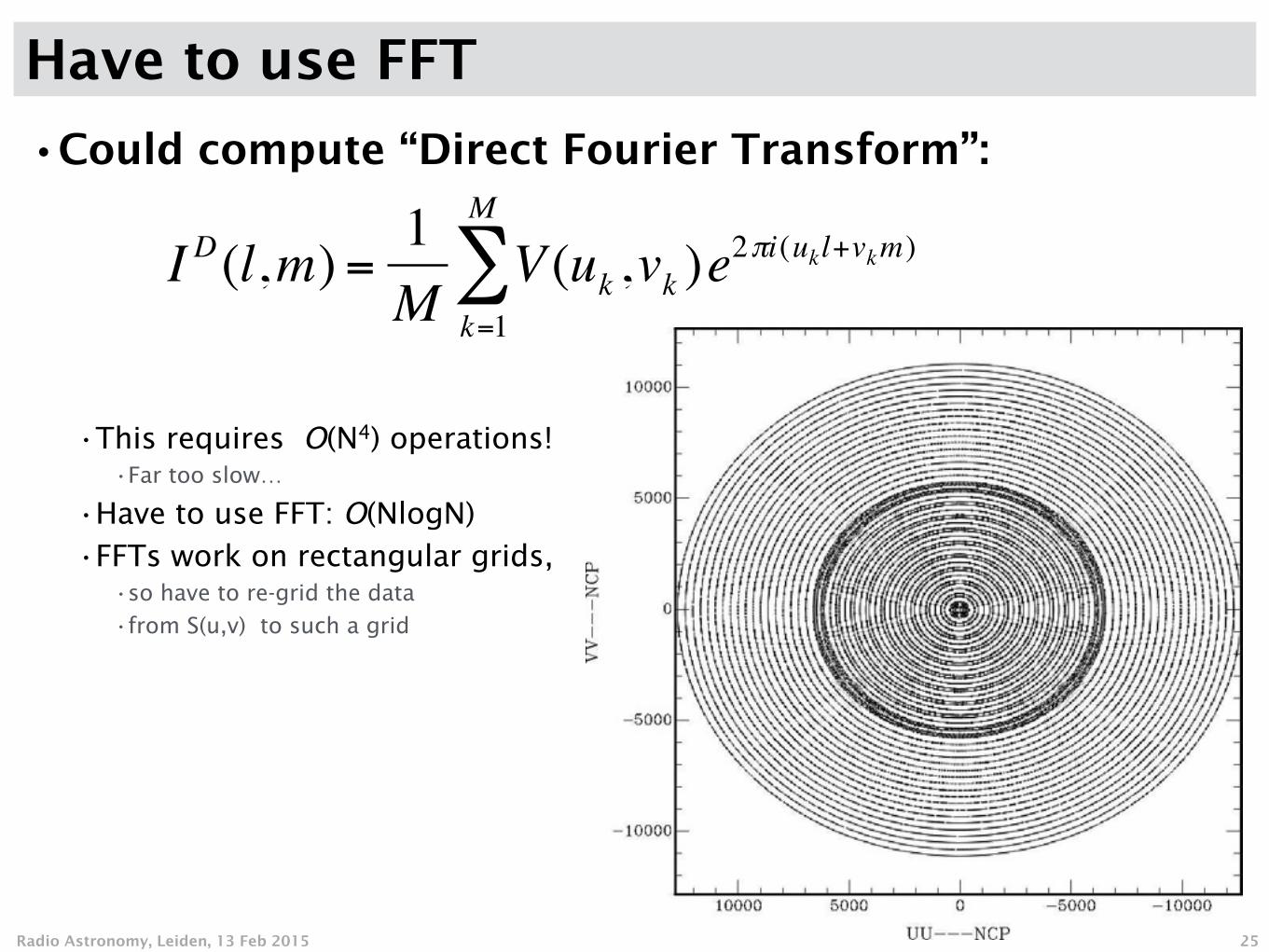
Have to use FFT
•Could compute “Direct Fourier Transform”:
!
!
!
!•This requires O(N4) operations!
•Far too slow…
•Have to use FFT: O(NlogN)
•FFTs work on rectangular grids, •so have to re-grid the data
•from S(u,v) to such a grid
25
€
I D(l,m) =1M
V (uk ,vk )e2πi(ukl+vkm)
k=1
M
∑ !
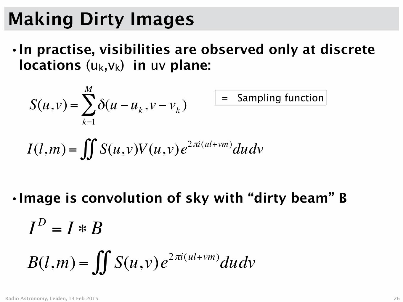
•In practise, visibilities are observed only at discrete locations (uk,vk) in uv plane:
!
!
!
!
!
!
•Image is convolution of sky with “dirty beam” B
/01Radio Astronomy, Leiden, 13 Feb 2015
Making Dirty Images
26
= Sampling function
€
S(u,v) = δ(u −uk ,v− vk )k=1
M
∑ !
€
I(l,m) = S(u,v)V∫∫ (u,v)e2πi(ul+vm )dudv !
€
I D = I ∗ B!
€
B(l,m) = S(u,v)∫∫ e2πi(ul+vm)dudv !
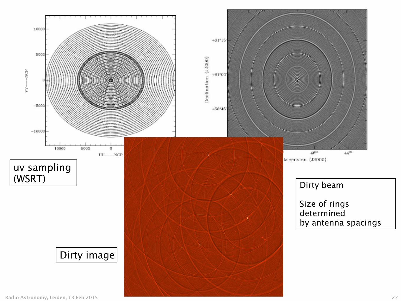
/01Radio Astronomy, Leiden, 13 Feb 2015 27
uv sampling (WSRT)
Dirty beam !Size of rings determined by antenna spacings
Dirty image
/01Radio Astronomy, Leiden, 13 Feb 2015
The classic Clean algorithm•Start with calculating the Beam
•Fourier transform of the u,v sampling
•Start an ImageModel •Which will be made of set of delta functions
•Algorithm: •1. Search for the peak in the dirty image.
•2. Add a fraction g (loop gain) of the peak value to ImageModel •(add delta-function to model).
•3. Subtract a scaled version of the PSF from the position of the peak.
!!
•4. If residuals are not “noise like”, goto 1.
•5. Smooth IM by an estimate of the main lobe (the “clean beam”) of the PSF and add the residuals to make the “restored image”2
!
•Many variations exist: •Clark clean: go back to discrete Visibilities in major cycles
•Multi-resolution: not just delta-functions
28
€
Ii+1R = Ii
R − g ⋅ B ⋅max(IiR )!
Högbom, 1974

/01Radio Astronomy, Leiden, 13 Feb 2015
Clean in action
29
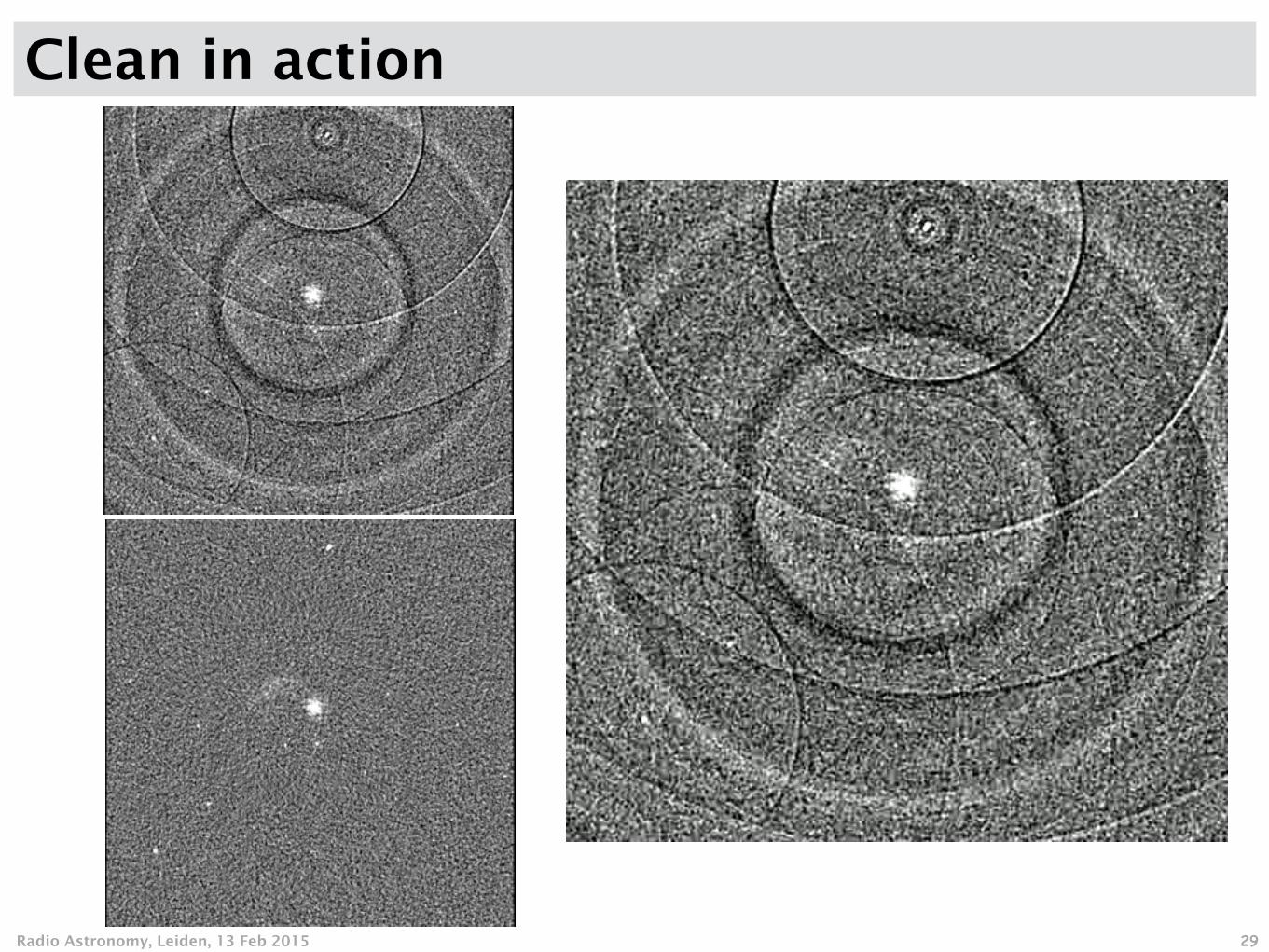
/01Radio Astronomy, Leiden, 13 Feb 2015
Clean in action
29

/01Radio Astronomy, Leiden, 13 Feb 2015
Clean in action
29
hu
ib 1
1/0
2/1
5
/33Radio Astronomy, Leiden, 13 Feb 2015
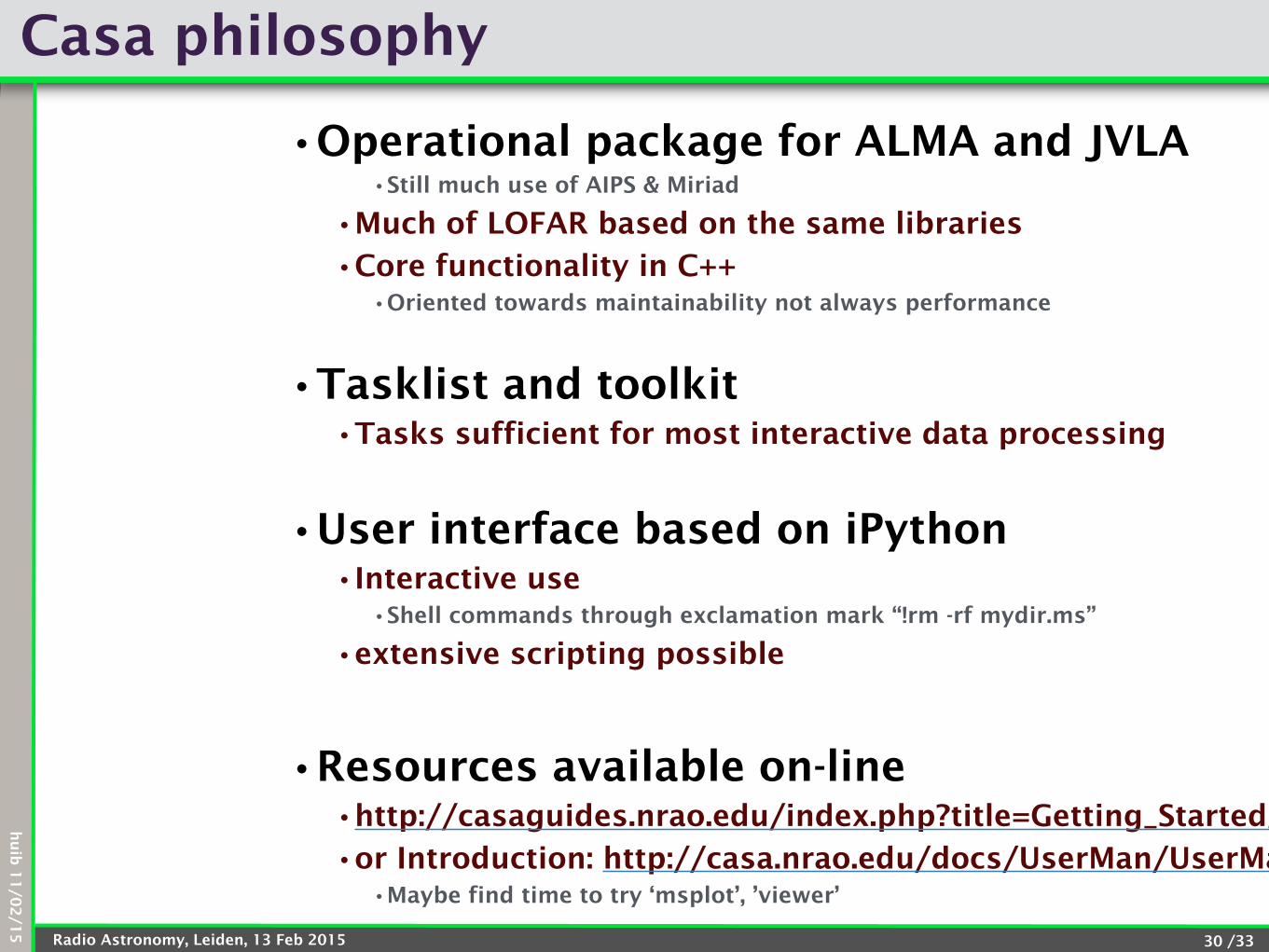
Casa philosophy
•Operational package for ALMA and JVLA •Still much use of AIPS & Miriad
•Much of LOFAR based on the same libraries
•Core functionality in C++ •Oriented towards maintainability not always performance
!•Tasklist and toolkit
•Tasks sufficient for most interactive data processing
!
•User interface based on iPython •Interactive use
•Shell commands through exclamation mark “!rm -rf mydir.ms”
•extensive scripting possible
!
•Resources available on-line •http://casaguides.nrao.edu/index.php?title=Getting_Started_in_CASA
•or Introduction: http://casa.nrao.edu/docs/UserMan/UserMan.html •Maybe find time to try ‘msplot’, ’viewer’
30
/01Radio Astronomy, Leiden, 13 Feb 2015
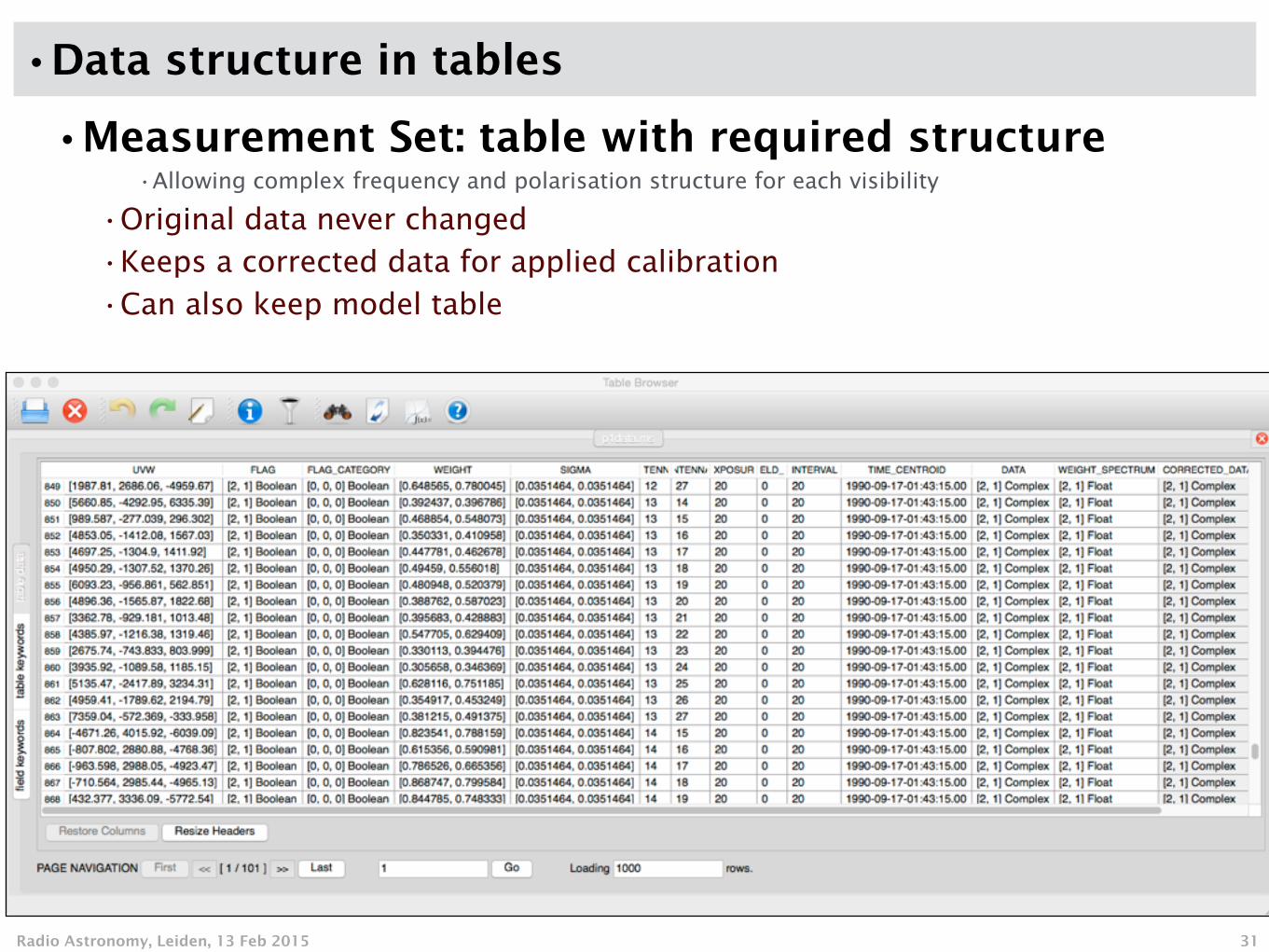
•Data structure in tables
•Measurement Set: table with required structure •Allowing complex frequency and polarisation structure for each visibility
•Original data never changed
•Keeps a corrected data for applied calibration
•Can also keep model table
31
hu
ib 1
1/0
2/1
5
/33Radio Astronomy, Leiden, 13 Feb 2015
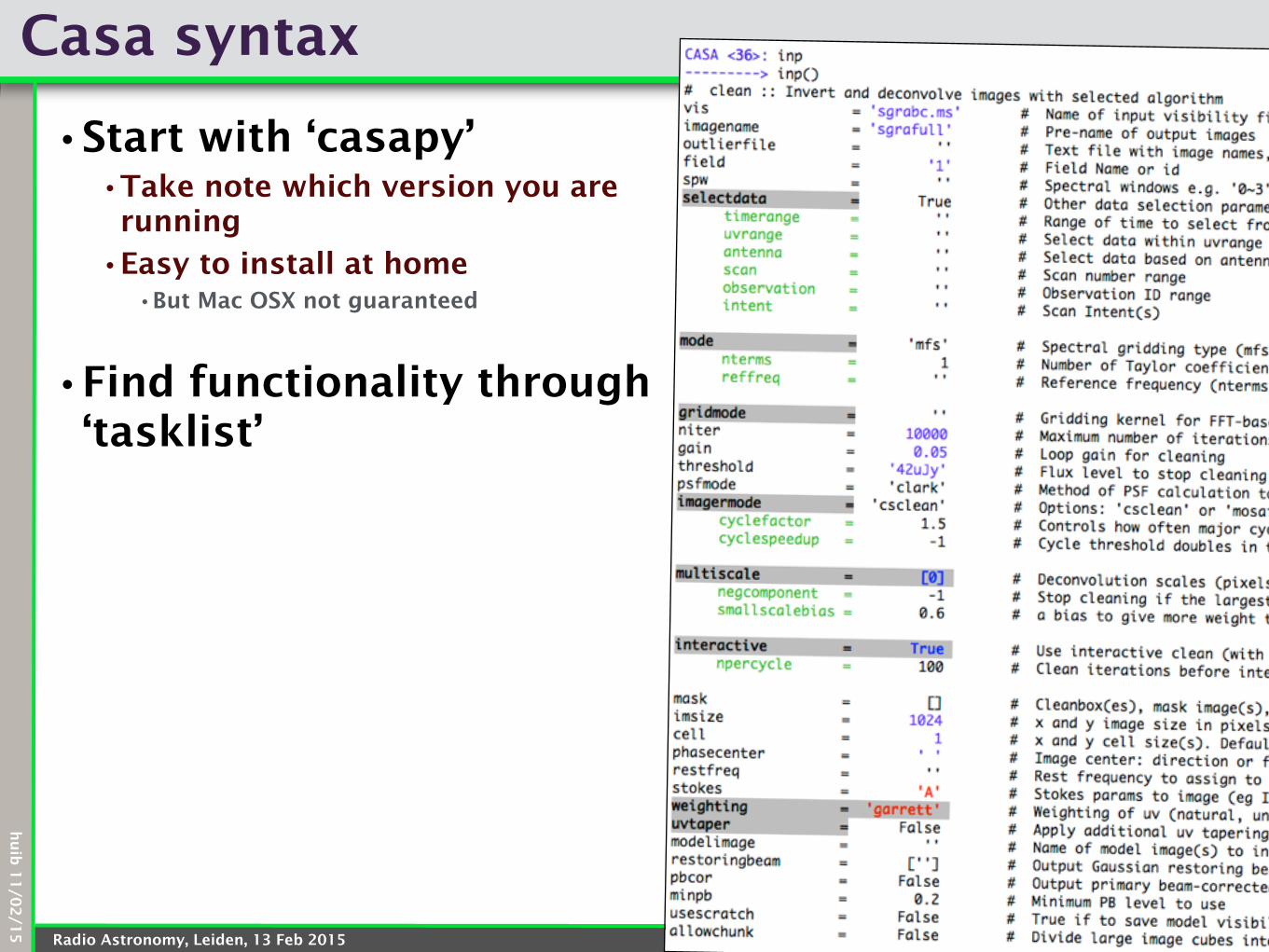
Casa syntax
•Start with ‘casapy’ •Take note which version you are
running
•Easy to install at home •But Mac OSX not guaranteed
!•Find functionality through
‘tasklist’
32
/01Radio Astronomy, Leiden, 13 Feb 2015
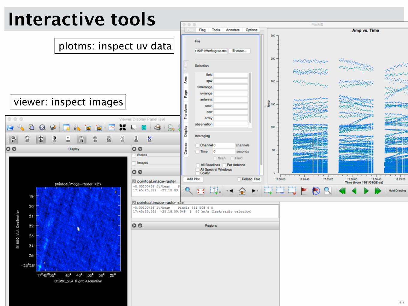
Interactive tools
33
viewer: inspect images
plotms: inspect uv data