Quasi stationary distributions.

P. Collet

Centre de Physique Theorique

CNRS UMR 7644

Ecole Polytechnique

F-91128 Palaiseau Cedex (France)

e-mail: collet@cpht.polytechnique.fr

Content of Lecture 1.

• The setting.

• A simple example of dynamical system.

• A simple example of Markov chain.

• General definitions.

• General results.

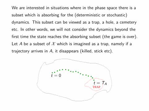
We are interested in situations where in the phase space there is a

subset which is absorbing for the (deterministic or stochastic)

dynamics. This subset can be viewed as a trap, a hole, a cemetery

etc. In other words, we will not consider the dynamics beyond the

first time the state reaches the absorbing subset (the game is over).

Let A be a subset of X which is imagined as a trap, namely if a

trajectory arrives in A, it disappears (killed, stick etc).

TRAP

t = 0

t = TA

For example in population dynamics, the number n of individuals of

a specie is an integer, the phase space is X = N∗ = 0, 1, 2, . . ..

Individuals can die, reproduce, for example in a birth and death

process. The number of individuals vary with time n(t). However

if there is no spontaneous generation, the state n = 0 is a trap, the

specie disappears at this state. If the system has reached that

state it stays there forever.

There are several natural questions associated to this setting.

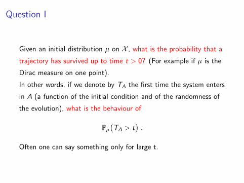
Question I

Given an initial distribution µ on X , what is the probability that a

trajectory has survived up to time t > 0? (For example if µ is the

Dirac measure on one point).

In other words, if we denote by TA the first time the system enters

in A (a function of the initial condition and of the randomness of

the evolution), what is the behaviour of

Pµ

(

TA > t)

.

Often one can say something only for large t.

Question II

Assume a trajectory initially distributed with µ has survived up to

time t > 0, what is the distribution of the state at time t?

In other words, can we say something about

Pµ

(

Xt ∈ B∣

∣TA > t)

=Pµ

(

Xt ∈ B , TA > t)

Pµ

(

TA > t) ,

B a measurable subset of X .

Question III

Are there trajectories which never reach the trap A? (TA = ∞).

If so, how are they distributed?

How is this related to Question II?

Question II (distribution of survivors at large time) deals with

trajectories which have survived for a large time but as we will see

later, most of them are on the verge of falling in the trap. This will

be the main subject of these lectures.

Question III deals with trajectories that will never see the trap, this

is very different.

Question II (distribution of survivors at large time) and Question

III (eternal life) have in general very different answers. This can be

seen clearly in the case of dynamical systems (deterministic time

evolution).

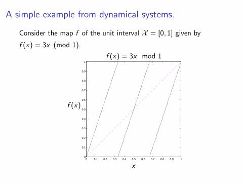
A simple example from dynamical systems.

Consider the map f of the unit interval X = [0, 1] given by

f (x) = 3x (mod 1).

0 0.1 0.2 0.3 0.4 0.5 0.6 0.7 0.8 0.9 10

0.1

0.2

0.3

0.4

0.5

0.6

0.7

0.8

0.9

1

x

f (x)

f (x) = 3x mod 1

It is easy to verify that the Lebesgue measure Leb is invariant,

namely for any Borel set B

Leb(

f −1(B))

= Leb(

B)

,

where f −1(B) is the preimage set of B , namely

f −1(B) =

x ∈ [0, 1]∣

∣ f (x) ∈ B

.

Given an initial distribution µ0 on [0, 1], and a map f of [0, 1], we

can define a discrete time stochastic process on [0, 1] as follows.

The probability space is [0, 1] and the process is defined recursively

by Xn+1 = f (Xn), X0 being distributed according to µ0.

The time evolution is deterministic, but the initial condition is

chosen at random. This randomness is propagated (here

“amplified”) by the time evolution.

We have a measure on the set of trajectories, this is a stochastic

process.

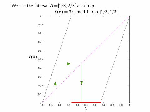
We use the interval A =]1/3, 2/3[ as a trap.

0 0.1 0.2 0.3 0.4 0.5 0.6 0.7 0.8 0.9 10

0.1

0.2

0.3

0.4

0.5

0.6

0.7

0.8

0.9

1

x

f (x)

f (x) = 3x mod 1 trap ]1/3, 2/3[

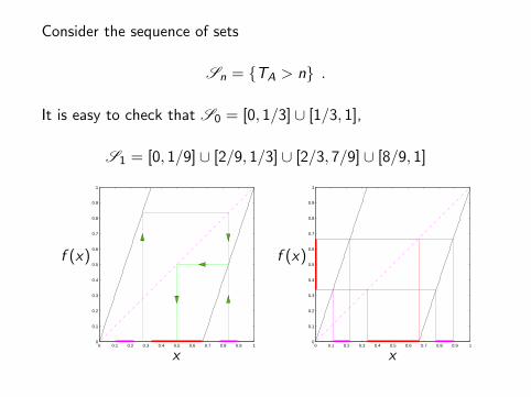
Consider the sequence of sets

Sn = TA > n .

It is easy to check that S0 = [0, 1/3] ∪ [1/3, 1],

S1 = [0, 1/9] ∪ [2/9, 1/3] ∪ [2/3, 7/9] ∪ [8/9, 1]

0 0.1 0.2 0.3 0.4 0.5 0.6 0.7 0.8 0.9 10

0.1

0.2

0.3

0.4

0.5

0.6

0.7

0.8

0.9

1

x

f (x)

0 0.1 0.2 0.3 0.4 0.5 0.6 0.7 0.8 0.9 10

0.1

0.2

0.3

0.4

0.5

0.6

0.7

0.8

0.9

1

x

f (x)

Consider the sequence of sets

Sn = TA > n .

It is easy to check that S0 = [0, 1/3] ∪ [1/3, 1],

S1 = [0, 1/9] ∪ [2/9, 1/3] ∪ [2/3, 7/9] ∪ [8/9, 1]

and so on. Therefore

Lebesgue(

Sn

)

=

(

2

3

)n+1

.

Namely we have the answer to question I: probability of surviving

up to time n starting from the Lebesgue measure. This probability

follows an exponential law.

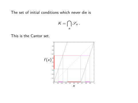
The set of initial conditions which never die is

K =⋂

n

Sn .

This is the Cantor set.

0 0.1 0.2 0.3 0.4 0.5 0.6 0.7 0.8 0.9 10

0.1

0.2

0.3

0.4

0.5

0.6

0.7

0.8

0.9

1

x

f (x)

The set of initial conditions which never die is

K =⋂

n

Sn .

This is the Cantor set.

K is of zero Lebesgue measure.

Moreover, during the recursive construction, if we start with the

Lebesgue measure, all the intervals of Sn have the same length

and hence the same weight. We get at the end the Cantor measure

which is very singular (absolutely singular with respect to the

Lebesgue measure).

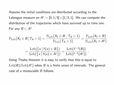
Assume the initial conditions are distributed according to the

Lebesgue measure on Ac = [0, 1/3]∪ [1/3, 1]. We can compute the

distribution of the trajectories which have survived up to time one.

For any B ⊂ Ac

PLeb

(

X1 ∈ B∣

∣TA > 1)

=PLeb

(

X1 ∈ B , TA > 1)

PLeb

(

TA > 1) =

PLeb

(

X1 ∈ B)

PLeb

(

X1 ∈ Ac)

=Leb

(

x∣

∣ f (x) ∈ B)

Leb(

x∣

∣ f (x) ∈ Ac) =

Leb(

f −1(B))

Leb(

f −1(Ac)) .

Using Thales theorem it is easy to verify that this is equal to

Leb(B)/Leb(Ac) when B is a finite union of intervals. The general

case of a measurable B follows.

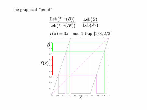
The graphical “proof”

Leb(

f −1(B))

Leb(

f −1(Ac)) =

Leb(B)

Leb(Ac)

0 0.1 0.2 0.3 0.4 0.5 0.6 0.7 0.8 0.9 10

0.1

0.2

0.3

0.4

0.5

0.6

0.7

0.8

0.9

1

x

f (x)

f (x) = 3x mod 1 trap ]1/3, 2/3[

B

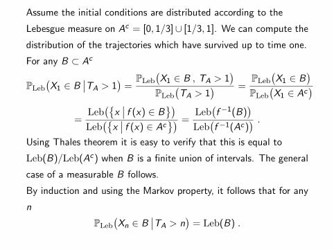
Assume the initial conditions are distributed according to the

Lebesgue measure on Ac = [0, 1/3]∪ [1/3, 1]. We can compute the

distribution of the trajectories which have survived up to time one.

For any B ⊂ Ac

PLeb

(

X1 ∈ B∣

∣TA > 1)

=PLeb

(

X1 ∈ B , TA > 1)

PLeb

(

TA > 1) =

PLeb

(

X1 ∈ B)

PLeb

(

X1 ∈ Ac)

=Leb

(

x∣

∣ f (x) ∈ B)

Leb(

x∣

∣ f (x) ∈ Ac) =

Leb(

f −1(B))

Leb(

f −1(Ac)) .

Using Thales theorem it is easy to verify that this is equal to

Leb(B)/Leb(Ac) when B is a finite union of intervals. The general

case of a measurable B follows.

By induction and using the Markov property, it follows that for any

n

PLeb

(

Xn ∈ B∣

∣TA > n)

= Leb(B) .

We have solved Question II (distribution of survivors at large time)

for the case of the (normalised) Lebesgue measure as initial

condition: the distribution stays Lebesgue.

Question III (survive forever) deals with trajectories that will never

see the trap. In the case of dynamical systems, these trajectories

concentrate on a very small set (a Cantor set) which is invariant

and disjoint from the trap.

Question II (distribution of survivors at large time) and Question

III (eternal life) have very different answers.

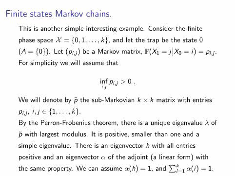
Finite states Markov chains.

This is another simple interesting example. Consider the finite

phase space X = 0, 1, . . . , k, and let the trap be the state 0

(A = 0). Let (pi ,j) be a Markov matrix, P(X1 = j∣

∣X0 = i) = pi ,j .

For simplicity we will assume that

infi ,j

pi ,j > 0 .

We will denote by p the sub-Markovian k × k matrix with entries

pi ,j , i , j ∈ 1, . . . , k.By the Perron-Frobenius theorem, there is a unique eigenvalue λ of

p with largest modulus. It is positive, smaller than one and a

simple eigenvalue. There is an eigenvector h with all entries

positive and an eigenvector α of the adjoint (a linear form) with

the same property. We can assume α(h) = 1, and∑k

i=1 α(i) = 1.

It is easy to verify that for 0 ≤ m ≤ n, x0, x ∈ 1, . . . , k

Px0

(

Xm = x , T0 > n)

=∑

y∈1,...,kpmx0,x p

n−mx ,y .

Therefore from spectral theory (pnx0,x = λn h(x0)α(x) + o(

λn)

)

Px0

(

T0 > n)

= λn h(x0) + o(

λn)

.

This is the answer to Question I: the survival probability decays

asymptotically exponentially fast. Moreover

limn→∞

Px0

(

Xn = x∣

∣T0 > n)

= α(x) .

This is the answer to Question II: the trajectories which have

survived up to time n (large) are asymptotically distributed

accordingly to the probability α.

For a fixed m ≥ 0

limn→∞

Px0

(

Xm = x∣

∣T0 > n)

= λ−m h(x)

h(x0)pm(x0, x)

This is the answer to Question III: the trajectories which survive

forever evolve according to a so called Q-process which is the

h-transform of p. This is a Markov process with transition

probabilities

λ−1 h(x)

h(x0)p(x0, x)

In particular, the invariant measure of the Q-process is the measure

µ with µ(x) = α(x) h(x), which in general is different from the

measure α.

We see the same phenomenon as in the case of dynamical systems

although less spectacular here.

One says that a probability measure ν is the Yaglom limit if for any

initial point x , and any Borel set B

limt→∞

Px

(

Xt ∈ B , TA > t)

Px

(

TA > t) = ν(B) .

A probability ν is a quasi limiting distribution (q.l.d.) if there is a

probability π such that in distribution

limt→∞

Pπ

(

Xt ∈ •∣

∣TA > t)

= ν(•) .

We say that ν (a probability on X ) is a quasi stationary

distribution (q.s.d.) if for any t ≥ 0

Pν

(

Xt ∈ B∣

∣TA > t)

= ν(B)

for any measurable set B . If there is no trap, this is a stationary

measure.

It is easy to prove using the Markov property that any q.l.d. is a

q.s.d. Any Yaglom limit is a q.l.d. (π = δx), hence a q.s.d.

There are few general results about q.s.d.

A first result concerns the entrance time TA in the trap A for a

Markov process(

Xt

)

.

Theorem 1

Let ν be a q.s.d. distribution for(

Xt

)

, then TA has an exponential

law, namely there is a number θ > 0 such that

Pν

(

TA > t)

= e−θt .

This result follows from the Markov property and the definition of

q.s.d. Note that this implies that for the q.s.d. most trajectories

which have survived up to time t will die very soon.

The case θ = 0 corresponds to invariant measure, and in the sequel

we will only consider θ > 0.

Proof of the exponential law.

One can verify by direct computations that this result holds in the

two previous examples. In the discrete time case we have

Pν

(

TA > n)

= Pν

(

X0 /∈ A, . . . ,Xn /∈ A)

= Pν

(

Xn /∈ A∣

∣X0 /∈ A, . . . ,Xn−1 /∈ A)

Pν

(

TA > n − 1)

and by the Markov property and stationarity

= Pν

(

Xn /∈ A∣

∣Xn−1 /∈ A)

Pν

(

TA > n − 1)

= Pν

(

X1 /∈ A∣

∣X0 /∈ A)

Pν

(

TA > n − 1)

= Pν

(

TA > 1)

Pν

(

TA > n − 1)

and the result follows by iteration.

The problem of existence of q.s.d. is in a sense similar to the

problem of existence of invariant measures.

There is however a supplementary difficulty: the rate of decay θ is

unknown (θ = 0 for invariant measures).

Up to now, no general existence theorem of q.s.d. is known, for

example there is nothing similar to the Krylov-Bogoliubov theorem

for stationary(invariant) measures.

We will see later on some particular results and techniques.

It is easy to construct examples where there is no q.s.d..

For example, if P(X1 ∈ A∣

∣X0 ∈ X\A) = 1, there cannot be any

q.s.d..

Indeed, here we have TA = 1 (almost surely!), but we have seen

before that if there is a q.s.d., this random variable should be

exponential.

Another less trivial example is given by the Brownian motion (Wt)

in dimension one with the trap A equal to the negative real line.

There is no Yaglom limit, no q.s.d..

One can show easily that (for x > 0)

Px

(

Wt ∈ [y , y+dy ] , T0 > t)

=1√2πt

(

e−(x−y)2/2t − e−(x+y)2/2t)

dy ,

hence

Px

(

T > t)

= x

√

2

πt+O

(

1

t3/2

)

,

no exponential decay. But there is renormalised Yaglom limit. It

follows by a short computation that

limt→∞

Px

(

Wt/√t ∈ [y , y + dy ]

∣

∣T0 > t)

= ye−y2/2dy .

The strategy to survive is to escape to infinity.

Some existence theorems in particular cases.

For continuous time Markov processes on countable phase space

(0, 1, 2, · · · , with trap 0), Ferrari Kesten Martinez and Picco

have proved the following result.

Theorem 2

Assume the process restricted to 1, 2, · · · is irreducible,

limx→∞ Px(T < t) = 0 for any t > 0 and Px(T <∞) = 1 for one

(and hence for all) x ∈ 1, 2, · · · . Then a necessary and sufficient

condition for the existence of a q.s.d. is

Ex

(

eλT)

<∞

for some λ > 0 and for one (hence for all) x ∈ 1, 2, · · · .

In a study of a birth and death process with mutation of the

phenotype, with S.Meleard, S.Martınez and J.San Martın, we came

to the following result.

Theorem 3

Let X be a polish space. Let S be a bounded positive linear

operator on C 0b (X ) the Banach space of bounded continuous

functions on X satisfying

S1 > c > 0 .

Assume there exists a continuous function ϕ ≥ 1 such that for any

u > 1, ϕ−1([1, u]) is compact and there exists D > 0 and γ ∈]0, c[such that for any ψ ∈ C 0

b (X ) with 0 ≤ ψ ≤ ϕ we have

Sψ ≤ γ ϕ+ D .

Then there exists a probability measure ν on X satisfying

S†ν = βν with β = ν(S1) > 0, (and ν(ϕ) <∞).

For continuous time, this result is used to prove the existence of a

q.s.d. by considering S = P1 where Pt is the semi-group

associated to the (killed) Makov process.

Example: birth and death processes. Let (an) and (bn) be two

sequences of strictly positive numbers, and consider the birth and

death process N(t) on N given by

P(

N(t + dt) = n + 1∣

∣N(t) = n)

= n an dt ,

P(

N(t + dt) = n − 1∣

∣N(t) = n)

= n bn dt ,

P(

|N(t + dt)− n| > 1∣

∣N(t) = n)

= 0 .

We assume no spontaneous generation, namely a0 = b0 = 0.

Theorem 4

Assume that

lim supn→∞

anbn

= β < 1 , and α = lim infn→∞

bn > 0 .

Then (N(t) has a q.s.d. (for the trap A = 0).

There are many ways to prove this theorem and one can get more

information on the q.s.d.(s) (see for example the recent review by

Van Doorn and Pollett). I will just illustrate how to use our

abstract result in this case. The proof is almost the same when

individuals carry phenotypic traits and birth can lead to mutations.

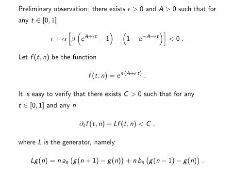
Preliminary observation: there exists ǫ > 0 and A > 0 such that for

any t ∈ [0, 1]

ǫ+ α[

β(

eA+ǫt − 1)

−(

1− e−A−ǫt)]

< 0 .

Let f (t, n) be the function

f (t, n) = en (A+ǫ t) .

It is easy to verify that there exists C > 0 such that for any

t ∈ [0, 1] and any n

∂t f (t, n) + Lf (t, n) < C ,

where L is the generator, namely

Lg(n) = n an(

g(n + 1)− g(n))

+ n bn(

g(n − 1)− g(n))

.

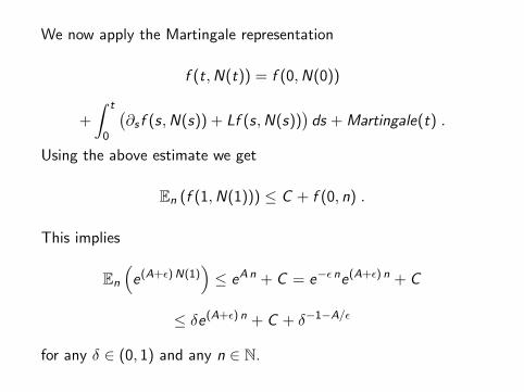
We now apply the Martingale representation

f (t,N(t)) = f (0,N(0))

+

∫ t

0

(

∂s f (s,N(s)) + Lf (s,N(s)))

ds +Martingale(t) .

Using the above estimate we get

En (f (1,N(1))) ≤ C + f (0, n) .

This implies

En

(

e(A+ǫ)N(1))

≤ eAn + C = e−ǫ ne(A+ǫ) n + C

≤ δe(A+ǫ) n + C + δ−1−A/ǫ

for any δ ∈ (0, 1) and any n ∈ N.

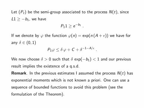
Let (Pt) be the semi-group associated to the process N(t), since

L1 ≥ −b1, we have

P11 ≥ e−b1 .

If we denote by ϕ the function ϕ(n) = exp(n (A+ ǫ)) we have for

any δ ∈ (0, 1)

P1ϕ ≤ δ ϕ+ C + δ−1−A/ǫ .

We now choose δ > 0 such that δ exp(−b1) < 1 and our previous

result implies the existence of a q.s.d.

Remark. In the previous estimates I assumed the process N(t) has

exponential moments which is not known a priori. One can use a

sequence of bounded functions to avoid this problem (see the

formulation of the Theorem).

A short bibliography

E. Van Doorn, P.Pollett. Quasi-stationary distributions. Memorandum

No. 1945, Department of Applied Mathematics, University of Twente

(2011).

P.Collet, S.Martınez, J. San Martın. Quasi-Stationary Distributions,

Stochastic Processes, Dynamical Systems, Applications. Prepared (2011).

P.Pollett. Quasi-stationary Distributions: A Bibliography.

www.maths.uq.edu.au/ pkp/papers/qsds/qsds.pdf

P.Ferrari, H.Kesten, S.Martınez, P.Picco. Existence of quasi-stationary

distributions. A renewal dynamical approach. Ann. Probab. 23, 501-521

(1995).

P.Collet, S.Meleard, S.Martınez and J.San Martın. Quasi-stationary

distributions for structured birth and death processes with mutations.

Probab. Th. and Rel. fields. 151, 191-231 (2011).

Q.S.D. for diffusions.

Content

• The setting.

• Bounded domain.

• Half line.

• The Ornstein Uhlenbeck process.

• Down from infinity.

We will consider diffusions which are solutions of a stochastic

differential equation

dX = α(X ) dt + dWt

where X ∈ Rn, α is a regular vector field on R

n. We will assume

that α satisfies the standard hypothesis so that the process (Xt) is

well defined for all (non negative) times. Many results below can

be extended to processes satisfying dX = α(X ) dt + σ(X ) dWt . In

order to simplify the exposition and for lack of time we will leave

to the interested reader this more general case.

We will only consider two cases: the case of a bounded domain B

in Rn with regular boundary (the trap is A = Bc), and the case

n = 1 (Xt ∈ R) with trap A = (−∞, 0].

Besides these cases, very few other situations have been studied

(Cattiaux-Meleard, Villemonais).

Bounded domain.

Let B be a bounded (nonempty) open connected domain in Rn

with regular boundary. The trap is A = Bc . The problem of q.s.d.

and Q-process in this case was studied by Pinsky.

The process (Xt)t∈R+ is well defined for X0 ∈ B , and we will study

its conditioning to the event T > t where T is the first time the

process hits the boundary of B .

Recall that the C0 semi-group (Pt) is defined on C 0(B) by

Pt f (x) = Ex

(

f (Xt)1T>t

)

.

Fix t > 0, then Pt is a continuous linear map of C 0(B). Moreover

the cone of non-negative functions in C 0(B) has nonempty

interior. Therefore by a theorem of Krein, there exists a probability

measure ν and a number λ ≥ 0 such that

P†1ν = λ ν .

By simple arguments it follows that there exists a q.s.d. (if λ > 0).

This abstract argument does not provide precise information,

although using that a q.s.d. is an eigenvector of the generator of

the semi group we obtain that it is absolutely continuous with a

regular density.

We will prove by other means (spectral theory)

Theorem 5

There is a unique q.s.d. and it is absolutely continuous with

respect to the Lebesgue measure.

Many more results follow from this approach: speed of

convergence, central limit theorem etc.

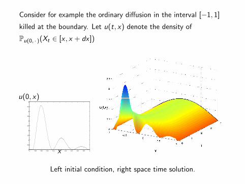
Consider for example the ordinary diffusion in the interval [−1, 1]

killed at the boundary. Let u(t, x) denote the density of

Pu(0, · )(Xt ∈ [x , x + dx ])

−1 −0.8 −0.6 −0.4 −0.2 0 0.2 0.4 0.6 0.8 10

0.5

1

1.5

2

2.5

3

3.5

4

4.5

5

x

u(0, x)

Left initial condition, right space time solution.

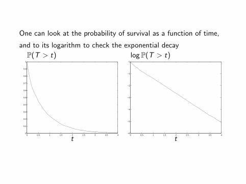
One can look at the probability of survival as a function of time,

and to its logarithm to check the exponential decay

0 0.5 1 1.5 2 2.5 3 3.5 40

0.1

0.2

0.3

0.4

0.5

0.6

0.7

0.8

0.9

1

t

P(T > t)

0 0.5 1 1.5 2 2.5 3 3.5 4−6

−5

−4

−3

−2

−1

0

t

logP(T > t)

We will use spectral theory of the associated semi-group Pt to

study q.s.d. and related properties.

Although the spectral theory of (Pt) can be studied in C 0(B), it is

slightly more convenient to work in L2(B). The relation is given by

the following Lemma.

Theorem 6

For any t > 0, Pt is a continuous map from L2(B) to C 0(B). (Pt)

extends to a C0 semi-group in L2(B).

Proof of the first part.

Let α be a smooth vector field with compact support, equal to α

in B , and (Xt) the process satisfying dX = α(X )dt + dWt . This

process coincides with (Xt) as long as (Xt) has not left B . For

f ≥ 0 in C 0(B), let f ≥ 0 be a continuous function with compact

support coinciding with f on B and satisfying

‖f ‖L2(Rn) ≤ 2‖f ‖L2(B). We have

Pt f (x) = Ex

(

f (Xt)1T>t(X.))

= Ex

(

f (Xt)1T>t(X.))

≤ Ex

(

f (Xt))

Girsanov= Ex

(

e∫ t

0 〈α(ws),dWs〉−1/2∫ t

0 α2(s)ds f (Wt)) Schwarz

≤

Ex

(

e2∫ t

0 〈α(ws),dWs〉−(1/2)∫ t

0 (2α)2(s)ds

)1/2Ex

(

e∫ t

0 α2(s)ds f 2(Wt))1/2

exp.martingale

≤ C te

(

1

(2πt)d/2

∫

Rn

e−(x−y)2/(2t) f 2(y) dy

)1/2

≤ C te‖f ‖L2(B)

and the proof of the first part follows by density of C 0(B) in L2(B).

Proof of the second part.

Note that in the above estimate, the constant is uniform on

compact sets in t.

Since the domain B is bounded, we have from the previous

inequality

‖Pt f ‖L2(B) ≤ C te∥

∥f∥

∥

L2(B),

with a constant uniform on compact sets in t. In other words, the

semi-group (Pt) is uniformly bounded in L2(B).

The C0 property in L2(B) follows from the density of C 0(B) in

L2(B) and a 3 ǫ argument.

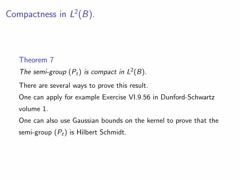
Compactness in L2(B).

Theorem 7

The semi-group (Pt) is compact in L2(B).

There are several ways to prove this result.

One can apply for example Exercise VI.9.56 in Dunford-Schwartz

volume 1.

One can also use Gaussian bounds on the kernel to prove that the

semi-group (Pt) is Hilbert Schmidt.

We will see later on that the spectral radius is strictly positive.

Hence the peripheral spectrum of any (Pt), is for t > 0 composed

of a finite number of points which are finite dimensional

eigenvalues. The rest of the spectrum lies in a closed disk of

smaller radius. The following result will be used several times in

the sequel. Let Br (y) denote the ball centered in y with radius r .

Lemma 8

For any r > 0, any t > 0, and any x , y ∈ B,

Pt1Br (y)(x) > 0 .

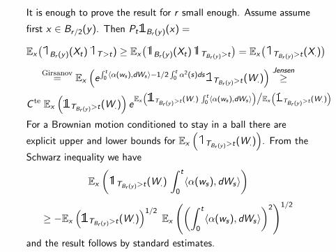
It is enough to prove the result for r small enough. Assume assume

first x ∈ Br/2(y). Then Pt1Br (y)(x) =

Ex

(

1Br (y)(Xt)1T>t) ≥ Ex

(

1Br (y)(Xt)1TBr (y)>t

)

= Ex

(

1TBr (y)>t(X.))

Girsanov= Ex

(

e∫ t

0 〈α(ws),dWs〉−1/2∫ t

0 α2(s)ds1TBr (y)>t(W.)

) Jensen≥

C teEx

(

1TBr (y)>t(W.))

eEx

(

1TBr (y)>t(W.)

∫ t

0 〈α(ws),dWs〉)/

Ex

(

1TBr (y)>t(W.)

)

For a Brownian motion conditioned to stay in a ball there are

explicit upper and lower bounds for Ex

(

1TBr (y)>t(W.))

. From the

Schwarz inequality we have

Ex

(

1TBr (y)>t(W.)

∫ t

0〈α(ws), dWs〉

)

≥ −Ex

(

1TBr (y)>t(W.))1/2

Ex

(

(∫ t

0〈α(ws), dWs〉

)2)1/2

and the result follows by standard estimates.

For x and y in B in general positions one can use a finite chain of

overlapping balls contained in B , “joining” x to y (recall that we

assumed B connected with regular boundary).

The following result is an important consequence.

Proposition 9

There is a function f0 in C 0(B) which is positive almost

everywhere and a number λ0 > 0 such that

Pt f0 = e−λ0t f0 .

This result is used to prove uniqueness of the q.s.d.

We now sketch the proof.

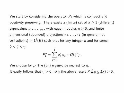
We start by considering the operator P1 which is compact and

positivity preserving. There exists a (finite) set of k ≥ 1 (different)

eigenvalues ρ1, . . . , ρk , with equal modulus η > 0, and finite

dimensional (bounded) projections π1, . . . , πk (in general not

self-adjoint) in L2(B) such that for any integer n and for some

0 < ζ < η

Pn1 =

k∑

j=1

ρnj πj +O(ζn) .

We choose for ρ1 the (an) eigenvalue nearest to η.

It easily follows that η > 0 from the above result Pt1Br (y)(x) > 0.

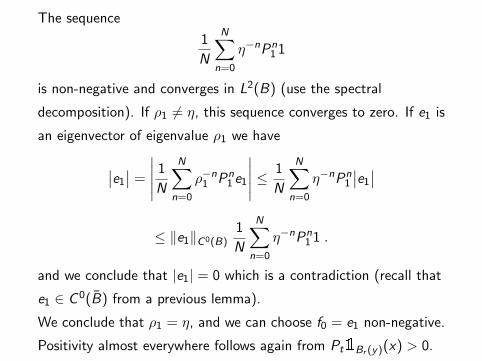
The sequence

1

N

N∑

n=0

η−nPn1 1

is non-negative and converges in L2(B) (use the spectral

decomposition). If ρ1 6= η, this sequence converges to zero. If e1 is

an eigenvector of eigenvalue ρ1 we have

∣

∣e1∣

∣ =

∣

∣

∣

∣

∣

1

N

N∑

n=0

ρ−n1 Pn

1 e1

∣

∣

∣

∣

∣

≤ 1

N

N∑

n=0

η−nPn1

∣

∣e1∣

∣

≤ ‖e1‖C0(B)1

N

N∑

n=0

η−nPn1 1 .

and we conclude that |e1| = 0 which is a contradiction (recall that

e1 ∈ C 0(B) from a previous lemma).

We conclude that ρ1 = η, and we can choose f0 = e1 non-negative.

Positivity almost everywhere follows again from Pt1Br (y)(x) > 0.

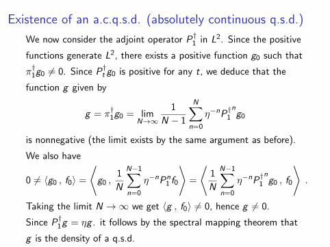
Existence of an a.c.q.s.d. (absolutely continuous q.s.d.)

We now consider the adjoint operator P†1 in L2. Since the positive

functions generate L2, there exists a positive function g0 such that

π†1g0 6= 0. Since P†t g0 is positive for any t, we deduce that the

function g given by

g = π†1g0 = limN→∞

1

N − 1

N∑

n=0

η−nP†1

ng0

is nonnegative (the limit exists by the same argument as before).

We also have

0 6= 〈g0 , f0〉 =⟨

g0 ,1

N

N−1∑

n=0

η−nPn1 f0

⟩

=

⟨

1

N

N−1∑

n=0

η−nP†1

ng0 , f0

⟩

.

Taking the limit N → ∞ we get 〈g , f0〉 6= 0, hence g 6= 0.

Since P†1g = ηg . it follows by the spectral mapping theorem that

g is the density of a q.s.d.

We now prove uniqueness.

We first observe that if ν is a q.s.d., since ν P1 = λν, and P1

maps L2 to C0, ν is a continuous linear functional on L2 and hence

absolutely continuous. We denote by g its density (note that g

also belongs to L1). Hence we have to prove uniqueness in L2.

Assume e1 and e ′1 are two independent non-negative eigenvectors

of P1 with eigenvalue η, which differ on a set of positive measure,

and such that∫

B

g e1 dx =

∫

B

g e ′1 dx = 1 .

Then, from P11Br (y)(x) > 0 and the continuity of e1 and e ′1η∣

∣e1 − e ′1∣

∣ =∣

∣P1e1 − P1e′1

∣

∣ < P1

∣

∣e1 − e ′1∣

∣ .

Integrating against g we get

η

∫

B

g∣

∣e1 − e ′1∣

∣ dx <

∫

B

g P1

∣

∣e1 − e ′1∣

∣ dx = η

∫

B

g∣

∣e1 − e ′1∣

∣ dx

a contradiction, hence the eigenvalue η of P1 is simple. The same

result holds for the adjoint P†1 , proving uniqueness of the q.s.d.

One can show more, namely that there is no other spectral point

on the circle of radius η.

This spectral gap implies an exponential rate of convergence in L2

for q.l.d. and Yaglom limits.

One can also give results on the regularity of the density of the

q.s.d., central limit theorem etc.

The Ornstein-Uhlenbeck process on R+.

This process provides an interesting example and was studied in

details by Lladser and San Martın. Recall that

dX = −X dt + dWt .

The trap is (−∞, 0].

Theorem 10 (Lladser San Martın)

For any θ ∈ (0, 1], there is a q.s.d. νθ absolutely continuous with

respect to the Lebesgue measure and such that

Pνθ

(

T > t)

= e−θ t .

In particular we see here that contrary to the case of bounded

domains, there is a continuum of q.s.d.

The densities uθ of these measures are related to special functions,

they are given by

uθ(x) = e−x2/2yθ(x)

where yθ is a parabolic cylinder function. In particular

u1(x) = 2xe−x2 .

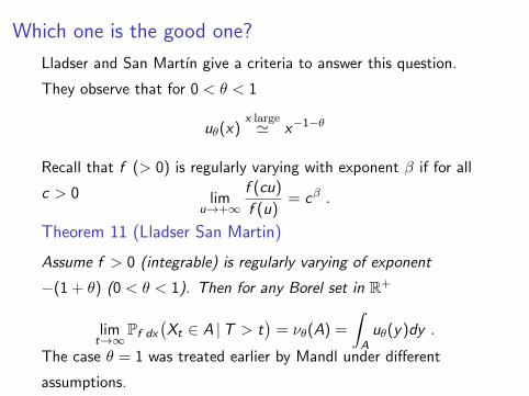
Which one is the good one?

Lladser and San Martın give a criteria to answer this question.

They observe that for 0 < θ < 1

uθ(x)x large≃ x−1−θ

Recall that f (> 0) is regularly varying with exponent β if for all

c > 0 limu→+∞

f (cu)

f (u)= cβ .

Theorem 11 (Lladser San Martin)

Assume f > 0 (integrable) is regularly varying of exponent

−(1 + θ) (0 < θ < 1). Then for any Borel set in R+

limt→∞

Pf dx

(

Xt ∈ A |T > t)

= νθ(A) =

∫

A

uθ(y)dy .

The case θ = 1 was treated earlier by Mandl under different

assumptions.

Down from infinity.

Why such a difference of behaviors between bounded and

unbounded domains: a continuum of q.s.d. versus one? This

seems to be related to the behavior of the drift near infinity.

Theorem 12

The process dZ = −Z 2dt + dWt on R+ (trap (−∞, 0]) has a

unique q.s.d. which is absolutely continuous with respect to

Lebesgue.

To prove this result we start by showing that this process comes

down from infinity very fast. This is not the case for the

Ornstein-Uhlenbeck process, which comes down from infinity but

not fast enough (the transition kernel from y to x is

z(t)−1 exp(−a(t)(x − b(t)y)2) with a(t) > 0 and 0 < b(t) < 1 for

t > 0).

Theorem 13

There exists a constant C > 0 such that for any x , y ∈ R+

Px

(

Z1 > y , T > 1)

≤ C e−√1+y

In order to prove this result, we will use the function

ϕ(t, x) = et√1+x .

It is easy to verify that for any x ≥ 0 and t ∈ [0, 1]

∂tϕ(t, x)− x2∂xϕ(t, x) +1

2∂2xϕ(t, x) ≤

(

2√t+ 1

)

ϕ .

From Ito’s formula it follows that for some constant C > 0, for any

x > 0 and t ∈ [0, 1]

Ex

(

ϕ(t,Zt)1T>t

)

≤ 1 +

∫ t

0

(

1 +2√s

)

Ex

(

ϕ(s,Zs)1T>s

)

ds .

It follows from Gronwall Lemma that Ex

(

ϕ(1,Z1)1T>1

)

<∞ and

the result follows by a Chebyshev inequality.

First consequence.

Theorem 14

There exists a q.s.d.

For the proof, apply Krein’s Theorem in C 0b (R

+) to the operator

P1. One gets a positive eigenvector ν in the dual space.

We have to prove the eigenvalue λ ≥ 0 is not zero. It is easy to

show that lim infx→∞ Px(T > 1) > 0. Since ν(P11) = λ ν(1), if

λ = 0 the functional is identically zero, a contradiction.

Finally the functional is a measure since tightness follows from the

previous estimate and the eigenvalue equation ν = λ−1 ν P1.

Second consequence.

Theorem 15

Let B = e√x/2C 0

b (R+) (this is a Banach space). The operator P1

is compact in B. The peripheral spectrum is finite and contains a

positive point which is a simple eigenvalue with positive

eigenvector.

For the proof, one first show that P1 extends to B using the

previous estimate. Better, P1 maps continuously B to C 0b (R

+).

Using Girsanov’s theorem one proves an estimate∣

∣P1f (x)∣

∣ ≤ C te x ‖f ‖B for x ∈ (0, 1]. On any compact interval (in

x) one uses Harnack regularity and compactness follows. The rest

of the theorem is proved as in the case of bounded domains.

Another proof relies on Gaussian bounds for the kernel in some

wheighted L2 space.

Third consequence.

Theorem 16

The q.s.d. is unique, a.c. with a continuous density.

By the q.s.d. equation, P†1ν = λ ν, a q.s.d. belongs to B∗, and we

know by the previous result that it is unique.

Moreover, in R+, the q.s.d. ν satisfies in the sense of distributions

1

2

d2

dx2ν +

d

dx

(

x2 ν)

= log(λ) ν

and therefore is a function.

As in the case of bounded domains, one can prove the existence of

a spectral gap etc.

Q.S.D. for Dynamical Systems.I will briefly explain one of the results: the Pianigiani Yorke

measure (for discrete time dynamical systems).

Theorem 17

Let T be a C 1+α map of Rn, and assume that there is an open set

Ω0 with compact closure such that

Ω0 ⊂ Int(

T (Ω0))

.

Assume there is a closed neighborhood V of Ω0 such that

supx∈V

∥

∥(DTx)−1‖ < 1 .

Then there is an a.c.q.s.d. ν for the trap A = Ω0c.

The result can be generalized in many directions, and one has

exponential convergence of q.l.d. (for adequate initial

distributions).

−2.5 −2 −1.5 −1 −0.5 0 0.5 1 1.5 2 2.5−2

−1.5

−1

−0.5

0

0.5

1

1.5

2

ℜ z

ℑ z

AΩ

0

Ω1

Ω∞

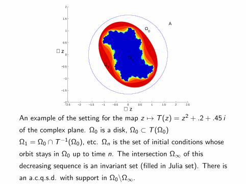
An example of the setting for the map z 7→ T (z) = z2 + .2 + .45 i

of the complex plane. Ω0 is a disk, Ω0 ⊂ T (Ω0)

Ω1 = Ω0 ∩ T−1(Ω0), etc. Ωn is the set of initial conditions whose

orbit stays in Ω0 up to time n. The intersection Ω∞ of this

decreasing sequence is an invariant set (filled in Julia set). There is

an a.c.q.s.d. with support in Ω0\Ω∞.

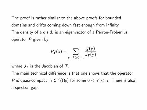
The proof is rather similar to the above proofs for bounded

domains and drifts coming down fast enough from infinity.

The density of a q.s.d. is an eigenvector of a Perron-Frobenius

operator P given by

Pg(x) =∑

y ,T (y)=x

g(y)

JT (y)

where JT is the Jacobian of T .

The main technical difference is that one shows that the operator

P is quasi-compact in Cα′

(Ω0) for some 0 < α′ < α. There is also

a spectral gap.

An example in numerical analysis: can you solve z3 = 1?

Yes! but we will test Newton’s method on this example. This

amounts to iterating the map

T (z) =2 z

3+

1

3 z2.

According to the choice of an initial condition, one converges to

one of the three roots of z3 = 1 which are the three (superstable)

fixed points of T or not.

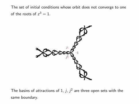
The set of initial conditions whose orbit does not converge to one

of the roots of z3 = 1.

1

j

j2

The basins of attractions of 1, j , j2 are three open sets with the

same boundary.

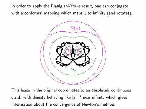
In order to apply the Pianigiani-Yorke result, one can conjugate

with a conformal mapping which maps 1 to infinity (and rotates).

u2u1

T(0 )

0

This leads in the original coordinates to an absolutely continuous

q.s.d. with density behaving like |z |−4 near infinity which gives

information about the convergence of Newton’s method.

A short bibliography

P.Cattiaux, P.Collet, A.Lambert, S.Martınez, S.Meleard , J.San Martın.

Quasi-stationary distributions and diffusions models in population

dynamics. Ann. Probab. 37, 1926-1969 (2009).

P.Collet, S.Martınez, J. San Martın. Quasi-Stationary Distributions,

Stochastic Processes, Dynamical Systems, Applications. Prepared (2011).

M.Lladser, J.San Martın. Domain of Attraction of the Quasi-stationary

distributions for the Ornstein-Uhlenbeck Process. Journal of Applied

Probability 37, 511-520 (2000).

T.Oikhberg, V.Troitsky. A theorem of Krein revisited. Rocky Mountain

J. Math. 35, 195-210 (2005).

R. Pinsky. On the convergence of diffusion processes conditioned to

remain in bounded region for large time to limiting positive recurrent

diffusion processes. Ann. Probab. 13, 363-378 (1985).

P.Pollett. Quasi-stationary Distributions: A Bibliography.

www.maths.uq.edu.au/ pkp/papers/qsds/qsds.pdf