Quantitative stability for the Brunn-Minkowski inequality

Alessio Figalli∗ and David Jerison†

Abstract

We prove a quantitative stability result for the Brunn-Minkowski inequality: if |A| = |B| = 1,t ∈ [τ, 1−τ ] with τ > 0, and |tA+(1−t)B|1/n ≤ 1+δ for some small δ, then, up to a translation,both A and B are quantitatively close (in terms of δ) to a convex set K.

1 Introduction

Given two sets A,B ⊂ Rn, and c > 0, we define the set sum and scalar multiple by

A+B := a+ b : a ∈ A, b ∈ B, cA := ca : a ∈ A (1.1)

Let |E| denote the Lebesgue measure of a set E (if E is not measurable, |E| denotes the outerLebesgue measure of E). The Brunn-Minkowski inequality states that, given A,B ⊂ Rn nonemptymeasurable sets,

|A+B|1/n ≥ |A|1/n + |B|1/n. (1.2)

In addition, if |A|, |B| > 0, then equality holds if and only if there exist a convex set K ⊂ Rn,λ1, λ1 > 0, and v1, v2 ∈ Rn, such that

λ1A+ v1 ⊂ K, λ2B + v2 ⊂ K, |K \ (λ1A+ v1)| = |K \ (λ2B + v2)| = 0.

Our aim is to investigate the stability of such a statement.

When n = 1, the following sharp stability result holds as a consequence of classical theorems inadditive combinatorics (an elementary proof of this result can be given using Kemperman’s theorem[C3, C4]):

Theorem 1.1. Let A,B ⊂ R be measurable sets. If |A + B| < |A| + |B| + δ for some δ ≤min|A|, |B|, then there exist two intervals I, J ⊂ R such that A ⊂ I, B ⊂ J , |I \ A| ≤ δ, and|J \B| ≤ δ.∗The University of Texas at Austin, Mathematics Dept. RLM 8.100, 2515 Speedway Stop C1200, Austin, TX

78712-1202 USA. E-mail address: figalli@math.utexas.edu†Department of Mathematics, Massachusetts Institute of Technology, 77 Massachusetts Ave, Cambridge, MA

02139-4307 USA. E-mail address: jerison@math.mit.edu

1

Concerning the higher dimensional case, in [C1, C2] M. Christ proved a qualitative stabilityresult for (1.2), namely, if |A+B|1/n is close to |A|1/n+|B|1/n then A and B are close to homotheticconvex sets.

On the quantitative side, first V. I. Diskant [D] and then H. Groemer [G] obtained some stabilityresults for convex sets in terms of the Hausdorff distance. More recently, sharp stability results interms of the L1 distance have been obtained by the first author together with F. Maggi and A.Pratelli [FMP1, FMP2]. Since this latter result will play a role in our proofs, we state it in detail.

We begin by noticing that, after dilating A and B appropriately, we can assume |A| = |B| = 1while replacing the sum A + B by a convex combination S := tA + (1 − t)B. It follows by (1.2)that |S| = 1 + δ for some δ ≥ 0.

Theorem 1.2. (see [FMP1, FMP2]) There is a computable dimensional constant C0(n) such thatif A,B ⊂ Rn are convex sets satisfying |A| = |B| = 1, |tA+(1− t)B| = 1+δ for some t ∈ [τ, 1− τ ],then, up to a translation,

|A∆B| ≤ C0(n)τ−1/2nδ1/2

(Here and in the sequel, E∆F denotes the symmetric difference between two sets E and F , that isE∆F = (E \ F ) ∪ (F \ E).)

Our main theorem here is a quantitative version of Christ’s result. His result relies on com-pactness and, for that reason, does not yield any explicit information about the dependence on theparameter δ. Since our proof is by induction on the dimension, it will be convenient to allow themeasures of |A| and |B| not to be exactly equal, but just close in terms of δ. Here is the mainresult of this paper, which shows that the measure of the difference between the sets A and B andtheir convex hull is bounded by a power δε, confirming a conjecture of Christ [C1].

Theorem 1.3. Let n ≥ 2, let A,B ⊂ Rn be measurable sets, and define S := tA + (1 − t)B forsome t ∈ [τ, 1− τ ], 0 < τ ≤ 1/2. There are computable dimensional constants Nn and computablefunctions Mn(τ), εn(τ) > 0 such that if∣∣|A| − 1

∣∣+∣∣|B| − 1

∣∣+∣∣|S| − 1

∣∣ ≤ δ (1.3)

for some δ ≤ e−Mn(τ), then there exists a convex set K ⊂ Rn such that, up to a translation,

A,B ⊂ K and |K \A|+ |K \B| ≤ τ−Nnδεn(τ).

Explicitly, we may take

Mn(τ) =23n+2

n3n | log τ |3n

τ3n, εn(τ) =

τ3n

23n+1n3n | log τ |3n.

It is interesting to make some comments on the above theorem: first of all, notice that the resultholds only under the assumption that δ is sufficiently small, namely δ ≤ e−Mn(τ). A smallnessassumption on δ is actually necessary, as can be easily seen from the following example:

A = B := Bρ(0) ∪ 2Le1,

2

where L 1, e1 denotes the first vector of the canonical basis in Rn, and ρ > 0 is chosen so that|Bρ(0)| = 1. Then it is easily checked that∣∣1

2A+ 12B∣∣ =

∣∣Bρ(0) ∪Bρ/2(Le1) ∪ 2Le1∣∣ = 1 + 2−n,

while | co(A)| ≈ L can be arbitrarily large, hence the result is false unless we assume that δ < 2−n.Concerning the exponent εn(τ), at the moment it is unclear to us whether a dimensional depen-

dency is necessary. It is however worth to point out that there are stability results for functionalinequalities where a dimensional dependent exponent is needed (see for instance [BP, Theorem 3.5]),so it would not be completely surprising if in this situation the optimal exponent does depend onn. We plan to investigate this very delicate question in future works.

Another important direction to develop would be to understand the analytic counterpart of theBrunn-Minkowski inequality, namely the Prekopa-Leindler inequality. At the moment, some sta-bility estimates are known only in one dimension or for some special class of functions [BB1, BB2],and a general stability result would be an important direction of future investigations.

The paper is structured as follows. In the next section we introduce a few notations and givean outline of the proof along with some commentary on the techniques and ideas. Then, in Section3 we collect most of the technical results we will use. Since the proofs of some of these technicalresults are delicate and involved, we postpone them to Section 5. Section 4 is devoted to the proofof Theorem 1.3.

Acknowledgements: AF was partially supported by NSF Grant DMS-1262411. DJ was partiallysupported by the Bergman Trust and NSF Grant DMS-1069225.

2 Notation and an outline of the proof

Let Hk denote k-dimensional Hausdorff measure on Rn. Denote by x = (y, s) ∈ Rn−1 × R a pointin Rn, and let π : Rn → Rn−1 and π : Rn → R denote the canonical projections, i.e.,

π(y, s) := y and π(y, s) := s.

Given a compact set E ⊂ Rn, y ∈ Rn−1, and λ > 0, we use the notation

Ey := E ∩ π−1(y) ⊂ y × R, E(s) := E ∩ π−1(s) ⊂ Rn−1 × s, (2.1)

E(λ) :=y ∈ Rn−1 : H1(Ey) > λ

. (2.2)

Following Christ [C2], we consider different symmetrizations.

Definition 2.1. Let E ⊂ Rn be a compact set. We define the Schwarz symmetrization E∗ of Eas follows. For each t ∈ R,

- If Hn−1(E(s)

)> 0, then E∗(s) is the closed disk centered at 0 ∈ Rn−1 with the same measure.

- If Hn−1(E(s)

)= 0, then E∗(s) is empty.

We define the Steiner symmetrization E? of E so that for each y ∈ Rn−1, the set E?y is empty ifH1(Ey) = 0; otherwise it is the closed interval of length H1(Ey) centered at 0 ∈ R. Finally, wedefine E\ := (E?)∗.

3

Outline of the proof of Theorem 1.3

The proof of Theorem 1.3 is very elaborate, combining the techniques of M. Christ with those de-veloped by the present authors in [FJ] (where we proved Theorem 1.3 in the special case A = B andt = 1/2), as well as several new ideas. For that reason, we give detailed description of the argument.

In Section 4.1 we prove the theorem in the special case A = A\ and B = B\. In this case wehave that

Ay = y × [−a(y), a(y)] and By = y × [−b(y), b(y)],

for some functions a, b : Rn−1 → R+, and it is easy to show that a and b satisfy the “3-pointconcavity inequality”

ta(y′) + (1− t)b(y′′) ≤ [ta+ (1− t)b](y) + δ1/4 (2.3)

whenever y′, y′′, and y := ty′ + (1 − t)y′′ belong to a large subset F of π(A) ∩ π(B). From this3-point inequality and an elementary argument (Remark 4.1) we show that a satisfies the “4-pointconcavity inequality”

a(y1) + a(y2) ≤ a(y′12) + a(y′′12) +2

tδ1/4 (2.4)

with y′12 := t′y1 + (1− t′)y2, y′′12 := t′′y1 + (1− t′′)y2, t′ := 12−t , t

′′ := 1− t′, provided all four pointsbelong to F . (The analogous inequality for b involves a different set of four points.)

Using this inequality and Lemma 3.6, we deduce that a is quantitatively close in L1 to a concavefunction. The proof, in Section 5, of Lemma 3.6, although reminiscent of Step 4 in the proof of[FJ, Theorem 1.2], is delicate and involved.

Once we know that a (and analogously b) is L1-close to a concave function, we deduce thatboth A and B are L1-close to convex sets KA and KB respectively, and we would like to say thatthese convex sets are nearly the same. This is demonstrated as part of Proposition 3.4, which isproved by first showing that S is close to tKA + (1− t)KB, then applying Theorem 1.2 to deducethat KA and KB are almost homothetic, and then constructing a convex set K close to A and Band containing both of them.

This concludes the proof of Theorem 1.3 in the case A = A\ and B = B\.

In Section 4.2 we consider the general case, which we prove in several steps, culminating ininduction on dimension.

Step 1. This first step is very close to the argument used by M. Christ in [C2], although ouranalysis is more elaborate since we have to quantify every estimate.

Given A, B, and S, as in the theorem, we consider their symmetrizations A\, B\, and S\, andapply the result from Section 4.1 to deduce that A\ and B\ are close to the same convex set. Thisinformation combined with Christ’s Lemma 3.1 allows us to deduce that functions y 7→ H1(Ay)and y 7→ H1(By) are almost equipartitioned (that is, the measure of their level sets A(λ) and B(λ)are very close). This fact combined with a Fubini argument yields that, for most levels λ, A(λ)and B(λ) are almost optimal for the (n−1)-dimensional Brunn-Minkowski inequality. Thus, by theinductive step, we can find a level λ ∼ δζ (ζ > 0) such that we can apply the inductive hypothesisto A(λ) and B(λ). Consequently, after removing sets of small measure both from A and B and

4

translating in y, we deduce that π(A), π(B) ⊂ Rn−1 are close to the same convex set.

Step 2. This step is elementary: we apply a Fubini argument and Theorem 1.1 to most ofthe sets Ay and By for y ∈ A(λ) ∩ B(λ) to deduce that they are close to their convex hulls.Note, however, that to apply Fubini and Theorem 1.1 it is crucial that, thanks to Step 1, wefound a set in Rn−1 onto which both A and B project almost fully. Indeed, in order to say thatH1(Ay + By) ≥ H1(Ay) +H1(By) it is necessary to know that both Ay and By are nonempty, asotherwise the inequality would be false!

Step 3. The argument here uses several ideas from our previous paper [FJ] to obtain a 3-pointconcavity inequality as in (2.3) above for the “upper profile” of A and B (and an analogous in-equality for the “lower profile”). This inequality allows us to say that the barycenter of Ay satisfiesthe 4-point inequality (2.4) both from above and from below, and from this information we candeduce that, as a function of y, the barycenter of Ay (resp. By) is at bounded distance from alinear function (see Lemma 5.1). It follows that the barycenters of Sy are a bounded distance froma linear function for a set S which is almost of full measure inside S. Then a variation of [FJ, Proofof Theorem 1.2, Step 3] allows us to show that, after an affine measure preserving transformation,S is universally bounded, that is, bounded in diameter by a constant of the form Cnτ

−Mn whereCn and Mn are dimensional constants.

Step 4. By a relatively easy argument we find sets A∼ and B∼ of the form

A∼ =⋃y∈Fy × [aA(y), bA(y)] B∼ =

⋃y∈Fy × [aB(y), bB(y)]

which are close to A and B, respectively, and are universally bounded.

Step 5. This is a crucial step: we want to show that A∼ and B∼ are close to convex sets. As inthe case A = A\ and B = B\, we would like to apply Lemma 3.6 to deduce that bA and bB (resp.aA and aB) are L1-close to concave (resp. convex) functions.

The main issue is that the hypothesis of the lemma, in addition to asking for boundednessand concavity of bA and bB at most points, also requires that the level sets of bA and bB be closeto their convex hulls. To deduce this we wish to show that most slices of A∼ and B∼ are nearlyoptimal in the Brunn-Minkowski inequality in dimension n−1 and invoke the inductive hypothesis.We achieve this by an inductive proof of the Brunn-Minkowski inequality, based on combining thevalidity of Brunn-Minkowski in dimension n− 1 with 1-dimensional optimal transport (see Lemma3.5).

An examination of this proof of the Brunn-Minkowski inequality in the situation near equalityshows that if A and B are almost optimal for the Brunn-Minkowski inequality in dimension n,then for most levels s, the slices A(s) and B(T (s)) have comparable (n − 1)-measure, where T isthe 1-dimensional optimal transport map, and this pair of sets is almost optimal for the Brunn-Minkowski inequality in dimension n− 1. In particular, we can apply the inductive hypothesis todeduce that most (n− 1)-dimensional slices are close to their convex hulls.

This nearly suffices to apply Lemma 3.6. But this lemma asks for control of the superlevel setsof the function bA, which a priori may be very different from the slices of A∼. To avoid this issue,

5

we simply replace A∼ and B∼ by auxiliary sets A− and B− which consist of the top profile of A∼

and B∼ with a flat bottom, so that the slices coincide with the superlevel sets of bA and bB. Wethen show that Lemma 3.5 applies to A− and B−. In this way, we end up proving that A∼ andB∼ are close to convex sets, as desired.

Step 6. Since A∼ and B∼ are close to A and B respectively, we simply apply Proposition 3.4as before in 4.1 to conclude the proof of the theorem.

Step 7. Tracking down the exponents in the proof, we provide an explicit lower (resp. upper)bound on εn(τ) (resp. Mn(τ)).

3 Technical Results

In this section we state most of the important lemmas we will need. The first three are due to M.Christ (or are easy corollaries of his results).

It is well-known that both the Schwarz and the Steiner symmetrization preserve the measureof sets, while they decrease the measure of the semi-sum (see for instance [C2, Lemma 2.1]). Also,as shown in [C2, Lemma 2.2], the \-symmetrization preserves the measure of the sets E(λ). Wecombine these results into one lemma, and refer to [C2, Section 2] for a proof.

Lemma 3.1. Let A,B ⊂ Rn be compact sets. Then |A| = |A∗| = |A?| = |A\|,

|tA∗+(1−t)B∗| ≤ |tA+(1−t)B|, |tA?+(1−t)B?| ≤ |tA+(1−t)B|, |tA\+(1−t)B\| ≤ |tA+(1−t)B|,

and, with the notation in (2.2),∣∣A \ π−1(A(λ)

)∣∣ =∣∣A\ \ π−1

(A\(λ)

)∣∣ and Hn−1(A(λ)

)= Hn−1

(A\(λ)

)for almost every λ > 0.

Another important fact is that a bound on the measure of tA+(1−t)B in terms of the measuresof A and B implies bounds relating the sizes of

supyH1(Ay), sup

yH1(By), Hn−1

(π(A)

), Hn−1

(π(B)

).

Lemma 3.2. Let A,B ⊂ Rn be compact sets such that |A|, |B| ≥ 1/2 and |tA+ (1− t)B| ≤ 2 forsome t ∈ (0, 1), and set τ := mint, 1− t There exists a dimensional constant M > 1 such that

supyH1(Ay)

supyH1(By)∈(τn

M,M

τn

),

Hn−1(π(A)

)Hn−1

(π(B)

) ∈ (τnM,M

τn

),

(supyH1(Ay)

)Hn−1

(π(A)

)∈(

1

M,M

τ2n

),

(supyH1(By)

)Hn−1

(π(B)

)∈(

1

M,M

τ2n

).

and, up a measure preserving affine transformation of the form (y, s) 7→ (λy, λ1−nt) with λ > 0, wehave

Hn−1(π(A)

)+Hn−1

(π(B)

)+ sup

yH1(Ay) + sup

yH1(By) ≤

M

τ2n. (3.1)

In this case, we say that A and B are (M, τ)-normalized.

6

Proof. As observed in [C2, Lemma 3.1] and in the discussion immediately after that lemma,(supyH1(Ay)

)Hn−1

(π(B)

)≤ |tA+ (1− t)B|

t(1− t)n−1≤ 2

τn,

(supyH1(Ay)

)Hn−1

(π(A)

)≥ |A| ≥ 1/2.

By exchanging the roles of A and B, the first part of the lemma follows. To prove the second part,it suffices to choose λ > 0 so that λn−1Hn−1

(π(A)

)= 1/τn.

The third lemma is a result of Christ [C1, Lemma 4.1] showing that supsHn−1(A(s)

)and

supsHn−1(B(s)

)are close in terms of δ:

Lemma 3.3. Let A,B ⊂ Rn be compact sets, define S := tA+ (1− t)B for some t ∈ [τ, 1− τ ], andassume that (1.3) holds for some δ ≤ 1/2. Then there exists a numerical constant L > 0 such that

supsHn−1(A(s)

)supsHn−1

(B(s)

) ∈ (1− Lτ−1/2δ1/2, 1 + Lτ−1/2δ1/2).

Proof. Set

γ :=

(supsHn−1

(A(s)

)supsHn−1

(B(s)

))1−t, γ :=

(supsHn−1

(B(s)

)supsHn−1

(A(s)

))t,and after possibly exchanging A and B, we may assume that γ ≤ 1. By the argument in the proofof [C1, Lemma 4.1] we get

|S| ≥ tγ−1|A|+ (1− t)γ−1|B|,

so, by (1.3), (tγ−1 + (1− t)γt/(1−t)

)− 1 ≤ 4δ.

The functionγ 7→ tγ−1 + (1− t)γt/(1−t)

is convex for γ ∈ (0, 1], attains its minimum at γ = 1, and its second derivative is bounded belowby τ . It follows that

4δ ≥(tγ−1 + (1− t)γt/(1−t)

)− 1 ≥ τ

2|γ − 1|2,

which proves the result.

There are several other important ingredients in the proof of Theorem 1.3, which are to ourknowledge new. Because their proofs are long and involved, we postpone them to Section 5.

The first of these results shows that if A and B are L1-close to convex sets KA and KB

respectively, then A and B are close to each other, and we can find a convex set K which containsboth A and B with a good control on the measure. As we shall see, the proof relies primarily onTheorem 1.2.

Proposition 3.4. Let A,B ⊂ Rn be compact sets, define S := tA+(1− t)B for some t ∈ [τ, 1− τ ],and assume that (1.3) holds. Suppose A,B ⊂ BR, for some R ≤ τ−Nn with Nn a dimensionalconstant Nn > 1. Suppose further that we can find a convex sets KA,KB ⊂ Rn such that

|A∆KA|+ |B∆KB| ≤ ζ (3.2)

7

for some ζ ≥ δ. Then there exists a dimensional constant Ln > 1 such that after a translation,

|A∆B| ≤ τ−Lnζ1/2n

and there exists a convex set K containing both A and B such that

|K \A|+ |K \B| ≤ τ−Lnζ1/2n3.

Our next result is a consequence of a proof of the Brunn-Minkowski inequality by induction,using horizontal (n− 1)-dimensional slices. The lemma says that when A, B, and S satisfy (1.3),then most of their horizontal slices (chosen at suitable levels) satisfy near equality in the Brunn-Minkowski inequality and the ratio of their volumes of the slices is comparable to 1 on a largeset.

Lemma 3.5. Given compact sets A,B ⊂ Rn and S := tA + (1 − t)B, and recalling the notationE(s) ⊂ Rn−1 × s in (2.1), we define the probability densities on the real line

ρA(s) :=Hn−1

(A(s)

)|A|

, ρB(s) :=Hn−1

(B(s)

)|B|

, ρS(s) :=Hn−1

(S(s)

)|S|

. (3.3)

Let T : R→ R be the monotone rearrangement sending ρA onto ρB, that is T is an increasing mapsuch that T]ρA = ρB.1 Then

|S| −(t|A|1/n + (1− t)|B|1/n

)n≥∫Ren−1(s)

(t+ (1− t)T ′(s)

)ds, (3.4)

where Tt(s) := ts+ (1− t)T (s) and

en−1(s) := Hn−1(S(Tt(s))

)−[tHn−1

(A(s)

)1/(n−1)+ (1− t)Hn−1

(B(T (s))

)1/(n−1)]n−1

.

Moreover, if t ∈ [τ, 1− τ ] and (1.3) holds with δ/τn is sufficiently small, then∫R

∣∣∣∣ ρA(s)

ρB(T (s))− 1

∣∣∣∣ ρA(s) ds ≤ C(n)

τn/2δ1/2. (3.5)

Finally, we have a lemma saying that if a function ψ is nearly concave on a large set, and mostof its level sets are close to their convex hulls, then it is L1-close to a concave function. Here andin the sequel, given a set E we will use co(E) to denote its convex hull.

1T] denotes the push-forward through the map T , that is,

T]ρA = ρB ⇔∫E

ρB(s) ds =

∫T−1(E)

ρA(s) ds ∀E ⊂ R Borel.

An explicit formula for T can be given using the distribution functions of ρA and ρB : if we define

GA(s) :=

∫ s

−∞ρA(s′) ds′, GB(s) :=

∫ s

−∞ρB(s′) ds′,

and we set G−1B (r) := infs ∈ R : GA(s) > t, then T = G−1

B GA.

8

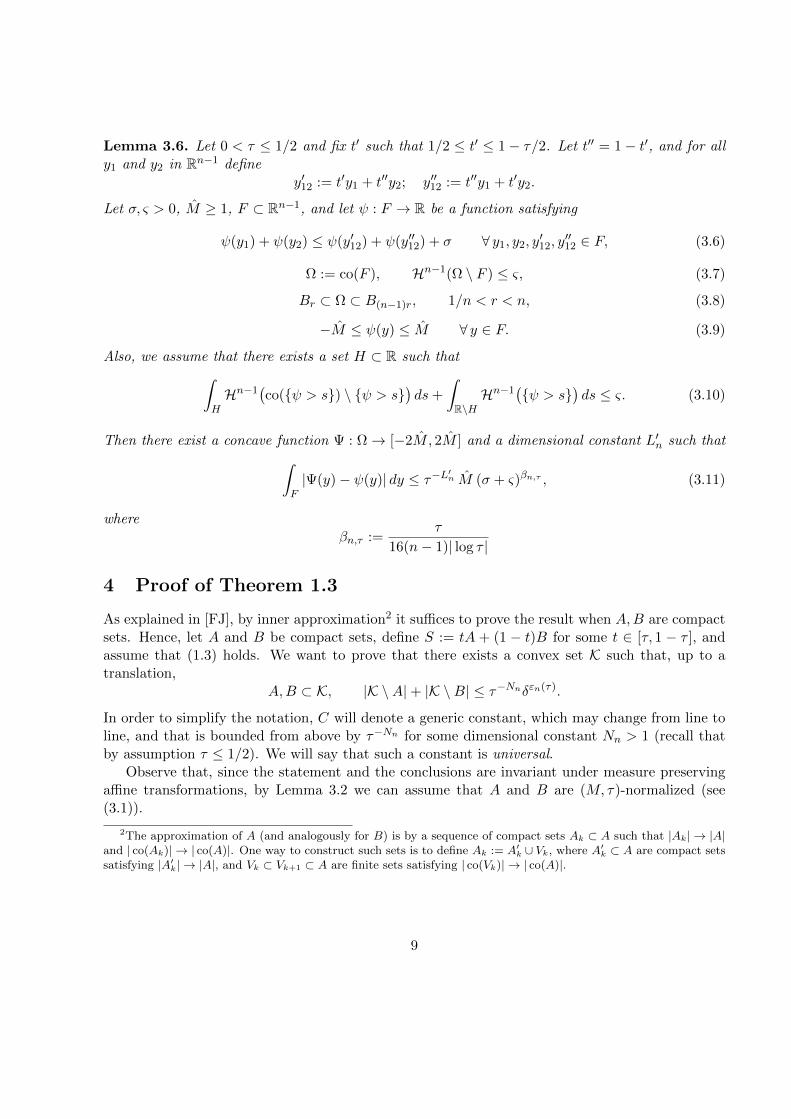
Lemma 3.6. Let 0 < τ ≤ 1/2 and fix t′ such that 1/2 ≤ t′ ≤ 1− τ/2. Let t′′ = 1− t′, and for ally1 and y2 in Rn−1 define

y′12 := t′y1 + t′′y2; y′′12 := t′′y1 + t′y2.

Let σ, ς > 0, M ≥ 1, F ⊂ Rn−1, and let ψ : F → R be a function satisfying

ψ(y1) + ψ(y2) ≤ ψ(y′12) + ψ(y′′12) + σ ∀ y1, y2, y′12, y

′′12 ∈ F, (3.6)

Ω := co(F ), Hn−1(Ω \ F ) ≤ ς, (3.7)

Br ⊂ Ω ⊂ B(n−1)r, 1/n < r < n, (3.8)

−M ≤ ψ(y) ≤ M ∀ y ∈ F. (3.9)

Also, we assume that there exists a set H ⊂ R such that∫HHn−1

(co(ψ > s) \ ψ > s

)ds+

∫R\HHn−1

(ψ > s

)ds ≤ ς. (3.10)

Then there exist a concave function Ψ : Ω→ [−2M, 2M ] and a dimensional constant L′n such that∫F|Ψ(y)− ψ(y)| dy ≤ τ−L′n M (σ + ς)βn,τ , (3.11)

whereβn,τ :=

τ

16(n− 1)| log τ |

4 Proof of Theorem 1.3

As explained in [FJ], by inner approximation2 it suffices to prove the result when A,B are compactsets. Hence, let A and B be compact sets, define S := tA + (1 − t)B for some t ∈ [τ, 1 − τ ], andassume that (1.3) holds. We want to prove that there exists a convex set K such that, up to atranslation,

A,B ⊂ K, |K \A|+ |K \B| ≤ τ−Nnδεn(τ).

In order to simplify the notation, C will denote a generic constant, which may change from line toline, and that is bounded from above by τ−Nn for some dimensional constant Nn > 1 (recall thatby assumption τ ≤ 1/2). We will say that such a constant is universal.

Observe that, since the statement and the conclusions are invariant under measure preservingaffine transformations, by Lemma 3.2 we can assume that A and B are (M, τ)-normalized (see(3.1)).

2The approximation of A (and analogously for B) is by a sequence of compact sets Ak ⊂ A such that |Ak| → |A|and | co(Ak)| → | co(A)|. One way to construct such sets is to define Ak := A′k ∪ Vk, where A′k ⊂ A are compact setssatisfying |A′k| → |A|, and Vk ⊂ Vk+1 ⊂ A are finite sets satisfying | co(Vk)| → | co(A)|.

9

4.1 The case A = A\ and B = B\

Let A,B ⊂ Rn be compact sets satisfying A = A\, B = B\. Since

π(A(s)

)⊂ π

(A(0)

)= π(A) and π

(B(s)

)⊂ π

(B(0)

)= π(B) are disks centered at the origin,

applying Lemma 3.3 we deduce that

Hn−1(π(A)∆π(B)

)≤ C δ1/2. (4.1)

Hence, if we define

S :=⋃

y∈π(A)∩π(B)

tAy + (1− t)By,

then Sy ⊂ Sy for all y ∈ Rn−1. In addition, using (1.3), (3.1), and (4.1), we have

1 + δ ≥ |S| =∫Rn−1

H1(Sy) dy ≥∫π(A)∩π(B)

H1(Sy) dy ≥∫π(A)∩π(B)

H1(Sy) dy

= |S| ≥ t∫π(A)∩π(B)

H1(Ay) dy + (1− t)∫π(A)∩π(B)

H1(By) dy

≥ t|A|+ (1− t)|B|2

− CHn−1(π(A)∆π(B)

)≥ 1− C δ1/2,

which implies (since S ⊂ S)|S \ S| ≤ C δ1/2. (4.2)

Also, by Chebyshev’s inequality we deduce that there exists a set F ⊂ π(A) ∩ π(B) such that

Hn−1((π(A) ∩ π(B)) \ F

)≤ C δ1/4, H1

(Sy \ Sy

)≤ δ1/4 ∀ y ∈ F.

This implies that, if we write

Ay := y × [−a(y), a(y)] and By := y × [−b(y), b(y)],

with a and b radial decreasing, then

ta(y′) + (1− t)b(y′′) ≤ [ta+ (1− t)b](y) + δ1/4 ∀ y = ty′ + (1− t)y′′, y, y′, y′′ ∈ F.

We show next that a three-point inequality for two functions f and g implies a four-point in-equality for each of f and g separately.

Remark 4.1. Let F ⊂ Rn−1, and f, g : F → R be two bounded Borel functions satisfying

tf(y′) + (1− t)g(y′′) ≤ [tf + (1− t)g](y) + σ ∀ y = ty′ + (1− t)y′′, y, y′, y′′ ∈ F,

for some σ ≥ 0. Let t ∈ [τ, 1− τ ] and define

t′ :=1

2− t, t′′ := 1− t′; y′12 := t′y1 + (1− t′)y2, y′′12 := t′′y1 + (1− t′′)y2 (4.3)

10

We claim that

f(y1) + f(y2) ≤ f(y′12) + f(y′′12) +2

tσ. (4.4)

(The analogous statement for g involves replacing t with 1 − t, so gives different values of t′ andt′′.) Notice that, if τ ≤ t ≤ 1/2, then

1/2 ≤ t′ ≤ 2/3 (4.5)

independent of τ , whereas if 1/2 ≤ t ≤ 1− τ , then

2/3 ≤ t′ ≤ 1− τ/2. (4.6)

To prove (4.4), note that the definitions above imply

y′12 = ty1 + (1− t)y′′12, y′′12 = ty′12 + (1− t)y2.

Hence, assuming that y1, y2, y′12, y

′′12 ∈ F , we can add together the two inequalities

tf(y1) + (1− t)g(y′′12) ≤ [tf + (1− t)g](y′12) + σ,

tf(y2) + (1− t)g(y′12) ≤ [tf + (1− t)g](y′′12) + σ,

to get (4.4).

By the remark above and Lemma 3.6 (notice that the level sets of a and b are both disks, so(3.10) holds with ς = 0), we obtain that both functions a and b are L1-close to concave functionsΨA and ΨB, both defined on π(A) ∩ π(B). Hence, if we define the convex sets

KA :=

(y, s) ∈ Rn : y ∈ π(A) ∩ π(B), −ΨA(y) ≤ s ≤ ΨA(y),

KB :=

(y, s) ∈ Rn : y ∈ π(A) ∩ π(B), −ΨB(y) ≤ s ≤ ΨB(y),

we deduce that|A∆KA|+ |B∆KB| ≤ C δβn,τ/4.

Hence, it follows from Proposition 3.4 that, up to a translation, there exists a convex set K suchthat A ∪B ⊂ K and

|A∆B| ≤ C δβn,τ/8n, |K \A|+ |K \B| ≤ C δβn,τ/8n3. (4.7)

Notice that, because A = A\ and B = B\, it is easy to check that the above properties still holdwith K\ in place of K. Hence, in this case, without loss of generality one can assume that K = K\.

4.2 The general case

Since the result is true when n = 1 (by Theorem 1.1), we assume that we already proved Theorem1.3 through n− 1, and we want to show its validity for n.

11

Step 1: There exist a dimensional constant ζ > 0 and λ ∼ δζ such that the inductivehypothesis applies to A(λ) and B(λ).

Let A\ and B\ be as in Definition 2.1. Thanks to Lemma 3.1, A\ and B\ still satisfy (1.3), so wecan apply the result proved in Section 4.1 above to get (see (4.7))∫

Rn−1

∣∣H1(A\y)−H1

(B\y

)∣∣ dy ≤ ∫Rn−1

∣∣H1(A\y∆B

\y

)∣∣ dy = |A\∆B\| ≤ C δα (4.8)

andK ⊃ A\ ∪B\, |K \A\|+ |K \B\| ≤ C δα/n2

(4.9)

for some convex set K = K\, where

α :=βn,τ8n

. (4.10)

In addition, because A and B are (M, τ)-normalized (see (3.1)), so are A\ and B\, and by (4.9) wededuce that there exists a universal constant R > 0 such that

K ⊂ BR. (4.11)

Also, by (4.8) and Chebyshev’s inequality we obtain that, up to a set of measure ≤ C δα/2,∣∣H1(A\y)−H1

(B\y

)∣∣ ≤ δα/2.Thus, recalling Lemma 3.1, for almost every λ > 0

Hn−1(A(λ)

)= Hn−1

(A\(λ)

)≤ Hn−1

(B\(λ− δα/2)

)+ C δα/2 = Hn−1

(B(λ− δα/2)

)+ C δα/2.

Since, by (3.1),∫ τ−2nM

0

(Hn−1

(B(λ)

)−Hn−1

(B(λ+ δα/2)

))dλ =

∫ δα/2

0Hn−1

(B(λ)

)dλ ≤ C δα/2,

by Chebyshev’s inequality we deduce that

Hn−1(A(λ)

)≤ Hn−1

(B(λ)

)+ C δα/4

for all λ outside a set of measure δα/4. Exchanging the roles of A and B we obtain that there existsa set G ⊂ [0, τ−2nM ] such that

H1(G) ≤ C δα/4,∣∣Hn−1

(A(λ)

)−Hn−1

(B(λ)

)∣∣ ≤ C δα/4 ∀λ ∈ [0,∞] \G. (4.12)

Using the elementary inequality(ta+ (1− t)b

)n−1≥ tan−1 + (1− t)bn−1 − C|a− b|2 ∀ 0 ≤ a, b ≤ M

τ2n,

and replacing a and b with a1/(n−1) and b1/(n−1), respectively, we get(ta1/(n−1) + (1− t)b1/(n−1)

)n−1≥ ta+ (1− t)b− C|a− b|2/(n−1) ∀ 0 ≤ a, b ≤ M

τ2n(4.13)

12

(notice that |a1/(n−1) − b1/(n−1)| ≤ |a− b|1/(n−1)). Finally, it is easy to check that

tA(λ) + (1− t)B(λ) ⊂ S(λ) ∀λ > 0.

Hence, by the Brunn-Minkowski inequality (1.2) applied to A(λ) and B(λ), using (1.3), (3.1), (4.13),and (4.12), we get

1 + δ ≥ |S| =∫ τ−2nM

0Hn−1

(S(λ)

)dλ

≥∫ τ−2nM

0

(tHn−1

(A(λ)

)1/(n−1)+ (1− t)Hn−1

(B(λ)

)1/(n−1))n−1

dλ

≥∫ τ−2nM

0

(tHn−1

(A(λ)

)+ (1− t)Hn−1

(B(λ)

))dλ

− C∫ τ−2nM

0

∣∣Hn−1(A(λ)

)−Hn−1

(B(λ)

)∣∣2/(n−1)dλ

= t|A|+ (1− t)|B| − C δα/[2(n−1)]

≥ 1− C δα/[2(n−1)].

(4.14)

We also observe that, since K = K\, by Lemma 3.1, (4.11), and [C2, Lemma 4.3], for almost everyλ > 0 we have ∣∣A \ π−1

(A(λ)

)∣∣ =∣∣A\ \ π−1

(A\(λ)

)∣∣≤∣∣K \ π−1

(K(λ)

)∣∣+M Hn−1(A\(λ)∆K(λ)

)≤ Cλ2 +M Hn−1(A\(λ)∆K(λ)),

(4.15)

and analogously for B. Also, by (4.9),∫ τ−2nM

0

(Hn−1

(A\(λ)∆K(λ)

)+Hn−1

(B\(λ)∆K(λ)

))dλ ≤ |K \A\|+ |K \B\| ≤ C δα/n2

. (4.16)

We set

η :=α

n2, (4.17)

and we notice that η ≤ min

α2(n−1) ,

α4

.

Take ζ > 0 to be fixed later. Then by (4.12), (4.14), (4.15), (4.16), and by Chebyshev’sinequality, we can find a level

λ ∈[

10 δζ

τ,20 δζ

τ

](4.18)

such that

Hn−1(S(λ)

)≤(tHn−1

(A(λ)

)1/(n−1)+ (1− t)Hn−1

(B(λ)

)1/(n−1))n−1

+ C δη−ζ , (4.19)

13

∣∣A \ π−1(A(λ)

)∣∣+∣∣B \ π−1

(B(λ)

)∣∣ ≤ C(δ2ζ + δη−ζ), (4.20)∣∣Hn−1

(A(λ)

)−Hn−1

(B(λ)

)∣∣ ≤ C δη. (4.21)

In addition, from the propertiesHn−1

(A(λ)

)≤ τ−2nM for any λ > 0 (see (3.1)),∫ τ−2nM

0 Hn−1(A(λ)

)dλ = |A| ≥ 1− δ,

λ 7→ Hn−1(A(λ)

)is a decreasing function,

we deduce thatτ2n

2M≤ Hn−1

(A(λ)

)≤ M

τ2n∀λ ∈

(0, τ2n(2M)−1

).

The same holds for B and S, hence

Hn−1(S(λ)

),Hn−1

(A(λ)

),Hn−1

(B(λ)

)∈[τ2n(2M)−1, τ−2nM

]provided δ ≤ τ−N for some large dimensional constant N . Set ρ := 1/Hn−1

(A(λ)

)1/(n−1) ∈[1/C,C], and define

A′ := ρA(λ), B′ := ρB(λ), S′ := ρS(λ).

By (4.19) and (4.21) we get

Hn−1(A′) = 1,∣∣Hn−1(B′)− 1

∣∣ ≤ C δη, Hn−1(S′) ≤ 1 + C δη−ζ .

while, by (1.2),

Hn−1(S′)1/(n−1) ≥ tHn−1(A′)1/(n−1) + (1− t)Hn−1(B′)1/(n−1) ≥ 1− C δη,

therefore ∣∣Hn−1(A′)− 1∣∣+∣∣Hn−1(B′)− 1

∣∣+∣∣Hn−1(S′)− 1

∣∣ ≤ C δη−ζ .Thus, by Theorem 1.3 applied with n − 1, up to a translation there exists a (n − 1)-dimensionalconvex set Ω′ such that

Ω′ ⊃ A′ ∪B′, Hn−1(Ω′ \A′

)+Hn−1

(Ω′ \B′

)≤ C δ(η−ζ)εn−1(τ).

Define ζ by

ζ :=εn−1(τ)

3η, (4.22)

and set Ω := Ω′/ρ. Then we obtain (recall that 1/ρ ≤ C and that εn−1(τ) ≤ 1)

Ω ⊃ A(λ) ∪ B(λ), Hn−1(Ω \ A(λ)

)+Hn−1

(Ω \ B(λ)

)≤ C δ2ζ . (4.23)

14

Step 2: Theorem 1.1 applies to most of the sets Ay and By for y ∈ A(λ) ∩ B(λ).

Define C := A(λ) ∩ B(λ) ⊂ S(λ). By (4.20), (4.23), (3.1), and (4.22), we have

|A \ π−1(C)|+ |B \ π−1(C)| ≤∣∣A \ π−1

(A(λ)

)∣∣+∣∣B \ π−1

(B(λ)

)∣∣+

∫(A(λ))\(B(λ))

H1(Ay) dy +

∫(B(λ))\(A(λ))

H1(By) dy

≤ C(δ2ζ + δη−ζ

)+ C

(Hn−1

(Ω \ A(λ)

)+Hn−1

(Ω \ B(λ)

))≤ C

(δ2ζ + δη−ζ

)≤ C δ2ζ

(4.24)

Hence, by (1.3) and (4.24),∫CH1(Sy \

(tAy + (1− t)By

))dy =

∫C

[H1(Sy)−H1(tAy + (1− t)By)

]dy

≤∫C

[H1(Sy)− tH1(Ay)− (1− t)H1(By)

]dy

= |S ∩ π−1(C)| − t|A ∩ π−1(C)| − (1− t)|B ∩ π−1(C)|≤ |S| − t|A| − (1− t)|B|+ t|A \ π−1(C)|+ (1− t)|B \ π−1(C)|≤ C δ2ζ .

(4.25)

Write C as C1 ∪ C2, where

C1 :=y ∈ C : H1(Sy)− tH1(Ay)− (1− t)H1(By) ≤ δζ

, C2 := C \ C1.

By Chebyshev’s inequalityHn−1

(C2

)≤ C δζ , (4.26)

while, recalling (4.18),

minH1(Ay),H1(By)

≥ λ > δζ/2 ∀ y ∈ C1.

Hence, by Theorem 1.1 applied to Ay, By ⊂ R for y ∈ C1, we deduce that

H1(co(Ay) \Ay

)+H1

(co(By) \By

)≤ C δζ (4.27)

(recall that co(E) denotes the convex hull of a set E). Let C1 ⊂ C1 denote the set of y ∈ C1 suchthat

H1(Sy \

(tAy + (1− t)By

))≤ δζ , (4.28)

and notice that, by (4.25) and Chebyshev’s inequality, Hn−1(C1 \ C1) ≤ C δζ . Then choose acompact set C1 ⊂ C1 such that Hn−1(C1 \ C1) ≤ δζ to obtain

Hn−1(C1 \ C1) ≤ C δζ . (4.29)

In particular, it follows from (4.23) that

Hn−1(Ω \ C1) ≤ C δζ . (4.30)

15

Step 3: There is S ⊂ S so that |S \ S| is small and S is bounded.

Define the compact sets

A :=⋃y∈C1

Ay, B :=⋃y∈C1

By, S :=⋃y∈C1

tAy + (1− t)By. (4.31)

Note that by (3.1), (4.24), (4.26), (4.29),

|A∆A|+ |B∆B| = |A \ π−1(C1)|+ |B \ π−1(C1)| ≤ Cδζ , (4.32)

therefore

|S| =∫C1H1(tAy + (1− t)By) dy ≥

∫C1

[tH1(Ay) + (1− t)H1(By)

]dy = t|A|+ (1− t)|B| ≥ 1−Cδζ .

Hence, by (1.3) (and S ⊂ S),|S∆S| ≤ Cδζ (4.33)

Next we show that S is bounded. First recall that

Sy =⋃

y=ty′+(1−t)y′′tAy′ + (1− t)By′′ , (4.34)

and by (4.28) we get

H1

(( ⋃y=ty′+(1−t)y′′

tAy′ + (1− t)By′′)\ tAy + (1− t)By

)≤ δζ ∀ y ∈ C1. (4.35)

Recalling that π : Rn → R is the orthogonal projection onto the last component (that is, π(y, s) =s), we define the characteristic functions

χAy (s) :=

1 if s ∈ π(tAy)0 otherwise,

χA,∗y (s) :=

1 if s ∈ π(t co(Ay))0 otherwise,

and analogously for By (with 1− t in place of t). Hence, by (4.27) we have the following estimateon the convolution of the functions χy and χ∗y:

‖χA,∗y′ ∗ χB,∗y′′ − χ

Ay′ ∗ χBy′′‖L∞(R) ≤ ‖χ

B,∗y′′ − χ

By′′‖L1(R) + ‖χA,∗y′ − χ

Ay′‖L1(R)

≤ H1(co(By′′) \By′′

)+H1

(co(Ay′) \Ay′

)< 3 δζ ∀ y′, y′′ ∈ C1.

(4.36)

Let us denote by [a, b] the interval π(t co(Ay′) + (1 − t) co(By′′)

), and notice that, since by con-

structionmin

tH1(Ay), (1− t)H1(By)

≥ minτ, 1− τλ ≥ 10 δζ ∀ y ∈ C1

(see (4.18)), this interval has length greater than 20 δζ . Also, it is easy to check that the functionχ∗y′ ∗χ∗y′′ is supported on [a, b], has slope equal to 1 (resp. −1) inside [a, a+ 3 δζ ] (resp. [b−3 δζ , b]),

16

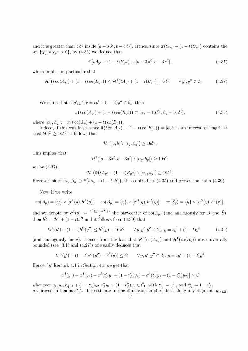
and it is greater than 3 δζ inside [a+ 3 δζ , b− 3 δζ ]. Hence, since π(tAy′ + (1− t)By′′

)contains the

set χy′ ∗ χy′′ > 0, by (4.36) we deduce that

π(tAy′ + (1− t)By′′

)⊃ [a+ 3 δζ , b− 3 δζ ], (4.37)

which implies in particular that

H1(t co(Ay′) + (1− t) co(By′′)

)≤ H1

(tAy′ + (1− t)By′′

)+ 6 δζ ∀ y′, y′′ ∈ C1. (4.38)

We claim that if y′, y′′, y = ty′ + (1− t)y′′ ∈ C1, then

π(t co(Ay′) + (1− t) co(By′′)

)⊂ [αy − 16 δζ , βy + 16 δζ ], (4.39)

where [αy, βy] := π(t co(Ay) + (1− t) co(By)

).

Indeed, if this was false, since π(t co(Ay′) + (1 − t) co(By′′)

)= [a, b] is an interval of length at

least 20δζ ≥ 16δζ , it follows that

H1([a, b] \ [αy, βy]

)≥ 16δζ .

This implies thatH1([a+ 3δζ , b− 3δζ ] \ [αy, by]

)≥ 10δζ ,

so, by (4.37),H1(π(tAy′ + (1− t)By′′

)\ [αy, βy]

)≥ 10δζ .

However, since [αy, βy] ⊃ π(tAy + (1− t)By

), this contradicts (4.35) and proves the claim (4.39).

Now, if we write

co(Ay) = y × [aA(y), bA(y)], co(By) = y × [aB(y), bB(y)], co(Sy) = y × [aS(y), bS(y)],

and we denote by cA(y) := aA(y)+bA(y)2 the barycenter of co(Ay) (and analogously for B and S),

then bS = tbA + (1− t)bB and it follows from (4.39) that

tbA(y′) + (1− t)bB(y′′) ≤ bS(y) + 16 δζ ∀ y, y′, y′′ ∈ C1, y = ty′ + (1− t)y′′ (4.40)

(and analogously for a). Hence, from the fact that H1(co(Ay)

)and H1

(co(By)

)are universally

bounded (see (3.1) and (4.27)) one easily deduces that∣∣tcA(y′) + (1− t)cB(y′′)− cS(y)∣∣ ≤ C ∀ y, y′, y′′ ∈ C1, y = ty′ + (1− t)y′′.

Hence, by Remark 4.1 in Section 4.1 we get that∣∣cA(y1) + cA(y2)− cA(t′Ay1 + (1− t′A)y2)− cA(t′′Ay1 + (1− t′′A)y2)∣∣ ≤ C

whenever y1, y2, t′Ay1 + (1− t′A)y2, t

′′Ay1 + (1− t′′A)y2 ∈ C1, with t′A := 1

2−t and t′′A := 1− t′A.As proved in Lemma 5.1, this estimate in one dimension implies that, along any segment [y1, y2]

17

on which C1 has large measure and such that y1, y2, t′Ay1 + (1− t′A)y2, t

′′Ay1 + (1− t′′A)y2 ∈ C1, cA is

at bounded distance from a linear function `A. Analogously,∣∣cB(y1) + cB(y2)− cB(t′By1 + (1− t′B)y2)− cB(t′′By1 + (1− t′′B)y2)∣∣ ≤ C

whenever y1, y2, t′By1 + (1 − t′B)y2, t

′′By1 + (1 − t′′B)y2 ∈ C1, now with t′B := 1

1+t and t′′B := 1 − t′B(recall again Remark 4.1), so cB is at bounded distance from a linear function `B along any segment[y1, y2] on which C1 has large measure and such that y1, y2, t

′By1 +(1− t′B)y2, t

′′By1 +(1− t′′B)y2 ∈ C1.

Hence, along any segment [y1, y2] on which C1 has large measure and such that y1, y2, t′Ay1 + (1−

t′A)y2, t′′Ay1 + (1− t′′A)y2, t

′By1 + (1− t′B)y2, t

′′By1 + (1− t′′B)y2 ∈ C1, cS is at bounded distance from

the linear function `(y) := t`A(y) + (1− t)`B(y).

We now use this information to deduce that, up to an affine transformation of the form

Rn−1 × R 3 (y, s) 7→ (Ty, t− Ly) + (y0, t0) (4.41)

with T : Rn−1 → Rn−1, det(T ) = 1, and (y0, t0) ∈ Rn, the set S is universally bounded, say S ⊂ BRfor some universal constant R.

Indeed, first of all, since C1 is almost of full measure inside the convex set Ω (see (4.23), (4.26),and (4.29)), by a simple Fubini argument (see the analogous argument in [FJ, Proof of Theorem1.2, Step 3-b] for more details) we can choose n “good” points y1, . . . , yn ∈ C1 such that:

(a) All points

y1, . . . , yn and t′Ay1 + (1− t′A)y2, t′′Ay1 + (1− t′′A)y2, t

′By1 + (1− t′B)y2, t

′′By1 + (1− t′′B)y2

belong to C1.

(b) Let Σi, i = 1, . . . , n, denote the (i − 1)-dimensional simplex generated by y1, . . . , yi, anddefine

Σ′i :=[t′AΣi+(1−t′A)yi+1

]∪[t′′AΣi+(1−t′′A)yi+1

]∪[t′BΣi+(1−t′B)yi+1

]∪[t′′BΣi+(1−t′′B)yi+1

],

i = 1, . . . , n− 1. Then

(i)

Hi−1(Σi) ≥ cn,Hi−1(Σi ∩ C1)

Hi−1(Σi)≥ 1− δζ/2, ∀ i = 2, . . . , n;

(ii)Hi−1

(Σ′i ∩ C1

)Hi−1 (Σ′i)

≥ 1− δζ/2 ∀ i = 2, . . . , n− 1.

Then, thanks to John’s Lemma [J], up to an affine transformation of the form (4.41) we can assumethat

Br ⊂ Ω ⊂ B(n−1)r, 1/Cn < r < Cn with Cn dimensional, (4.42)

and(yk, 0) ∈ S, ∀ k = 1, . . . , n . (4.43)

18

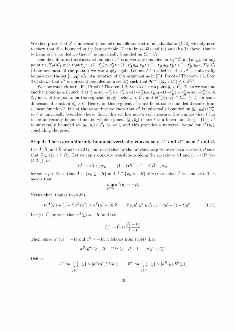
We then prove that S is universally bounded as follows: first of all, thanks to (4.42) we only needto show that S is bounded in the last variable. Then, by (4.43) and (a) and (b)-(i) above, thanksto Lemma 5.1 we deduce that cS is universally bounded on Σ2 ∩ C1.

One then iterates this construction: since cS is universally bounded on Σ2∩C′1 and at y3, for anypoint z ∈ Σ2∩C1 such that t′Az+(1−t′A)y3, t

′′Az+(1−t′′A)y3, t

′Bz+(1−t′B)y3, t

′′Bz+(1−t′′B)y2 ∈ Σ′2∩C1

(these are most of the points) we can apply again Lemma 5.1 to deduce that cS is universallybounded on the set [z, y3]∩ C1. An iteration of this argument as in [FJ, Proof of Theorem 1.2, Step3-d] shows that cS is universal bounded on a set Σ′′n such that Hn−1(Σn \ Σ′′n) ≤ C δζ/2.

We now conclude as in [FJ, Proof of Theorem 1.2, Step 3-e]: fix a point y1 ∈ C1. Then we can findanother point y2 ∈ C1 such that t′Ay1+(1−t′A)y2, t

′′Ay1+(1−t′′A)y2, t

′B y1+(1−t′B)y2, t

′′B y1+(1−t′′B)y2 ∈

C1, most of the points on the segment [y1, y2] belong to C1, and H1([y1, y2] ∩ Σ′′n

)≥ c′n for some

dimensional constant c′n > 0. Hence, on this segment cS must be at some bounded distance froma linear function `, but at the same time we know that cS is universally bounded on [y1, y2] ∩ Σ′′n,so ` is universally bounded there. Since this set has non-trivial measure, this implies that ` hasto be universally bounded on the whole segment [y1, y2] (since ` is a linear function). Thus cS

is universally bounded on [y1, y2] ∩ C1 as well, and this provides a universal bound for cS(y1),concluding the proof.

Step 4: There are uniformly bounded vertically convex sets A∼ and B∼ near A and B.

Let A, B, and S be as in (4.31), and recall that by the previous step there exists a constant R suchthat S ⊂ |xn| ≤ R. Let us apply opposite translations along the en-axis to tA and (1− t)B (see(4.31)), i.e.,

tA 7→ tA+ µen, (1− t)B 7→ (1− t)B − µen,

for some µ ∈ R, so that A ⊂ xn ≥ −R and A ∩ xn = −R 6= ∅ (recall that A is compact). Thismeans that

miny∈C1

aA(y) = −R.

Notice that, thanks to (4.39),

taA(y′) + (1− t)aB(y′′) ≥ aS(y)− 16 δζ ∀ y, y′, y′′ ∈ C1, y = ty′ + (1− t)y′′. (4.44)

Let y ∈ C1 be such that aA(y) = −R, and set

C−1 := C1 ∩C1 − ty1− t

.

Then, since aA(y) = −R and aS ≥ −R, it follows from (4.44) that

aB(y′′) ≥ −R− C δζ ≥ −R− 1 ∀ y′′ ∈ C−1 .

DefineA∼ :=

⋃y∈C−1

y × [aA(y), bA(y)], B∼ :=⋃y∈C−1

y × [aB(y), bB(y)].

19

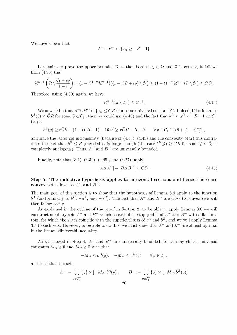
We have shown thatA∼ ∪B∼ ⊂ xn ≥ −R− 1.

It remains to prove the upper bounds. Note that because y ∈ Ω and Ω is convex, it followsfrom (4.30) that

Hn−1

(Ω \ C1 − ty

1− t

)= (1− t)1−nHn−1

(((1− t)Ω + ty) \ C1

)≤ (1− t)1−nHn−1(Ω \ C1) ≤ C δζ .

Therefore, using (4.30) again, we have

Hn−1(Ω \ C−1 ) ≤ C δζ . (4.45)

We now claim that A∼∪B∼ ⊂ xn ≤ CR for some universal constant C. Indeed, if for instancebA(y) ≥ CR for some y ∈ C−1 , then we could use (4.40) and the fact that bB ≥ aB ≥ −R− 1 on C−1to get

bS(y) ≥ tCR− (1− t)(R+ 1)− 16 δζ ≥ τCR−R− 2 ∀ y ∈ C1 ∩ (ty + (1− t)C−1 ),

and since the latter set is nonempty (because of (4.30), (4.45) and the convexity of Ω) this contra-dicts the fact that bS ≤ R provided C is large enough (the case bB(y) ≥ CR for some y ∈ C1 iscompletely analogous). Thus, A∼ and B∼ are universally bounded.

Finally, note that (3.1), (4.32), (4.45), and (4.27) imply

|A∆A∼|+ |B∆B∼| ≤ Cδζ . (4.46)

Step 5: The inductive hypothesis applies to horizontal sections and hence there areconvex sets close to A∼ and B∼.

The main goal of this section is to show that the hypotheses of Lemma 3.6 apply to the functionbA (and similarly to bB, −aA, and −aB). The fact that A∼ and B∼ are close to convex sets willthen follow easily.

As explained in the outline of the proof in Section 2, to be able to apply Lemma 3.6 we willconstruct auxiliary sets A− and B− which consist of the top profile of A∼ and B∼ with a flat bot-tom, for which the slices coincide with the superlevel sets of bA and bB, and we will apply Lemma3.5 to such sets. However, to be able to do this, we must show that A− and B− are almost optimalin the Brunn-Minkowski inequality.

As we showed in Step 4, A∼ and B∼ are universally bounded, so we may choose universalconstants MA ≥ 0 and MB ≥ 0 such that

−MA ≤ aA(y), −MB ≤ aB(y) ∀ y ∈ C−1 ,

and such that the sets

A− :=⋃y∈C−1

y × [−MA, bA(y)], B− :=

⋃y∈C−1

y × [−MB, bB(y)],

20

are universally bounded. We may also adjust the constants MA and MB so that |A−| = |B−|.Define

S− := tA− + (1− t)B−; C−(y) := (y′, y′′) ∈ C− × C− : ty′ + (1− t)y′′ = y.

We estimate the measure of S− using (4.40) as follows:

|S−| =∫tC−1 +(1−t)C−1

H1

( ⋃(y′,y′′)∈C−(y)

t[−MA, bA(y′)] + (1− t)[−MB, b

B(y′′)]

)dy

≤∫tC−1 +(1−t)C−1

(bS(y) + 16 δζ + tMA + (1− t)MB

)dy

≤∫C−1

(bS(y) + tMA + (1− t)MB

)dy + C δζ ,

where, in the final inequality, we used that Hn−1((tC−1 + (1 − t)C−1 ) \ C−1

)≤ C δζ (recall that

C−1 ⊂ Ω and Ω is convex, thus tC−1 + (1− t)C−1 ⊂ Ω and the bound follows from (4.45)) and that bS

is universally bounded on C−1 . Next, since bS = tbA + (1− t)bB and |A−| = |B−|, it follows that

|S−| ≤ t∫C−1

(bA(y)−MA) dy + (1− t)∫C−1

(bB(y)−MB) dy + C δζ

= t|A−|+ (1− t)|B−|+ C δζ = |A−|+ C δζ ,

On the other hand (1.2) implies

|S−| ≥(t|A−|1/n + (1− t)|B−|1/n

)n= |A−|.

Hence, in all, we find that

0 ≤ |S−| − |A−| ≤ C δζ and |A−| = |B−| (4.47)

We are now in a position to apply Lemma 3.5 to A− and B− to confirm that hypothesis (3.10) ofLemma 3.6 is valid for bA and bB.

Let us recall the notation E(s) ⊂ Rn−1 × s in (2.1). Since |cA−| = |cB−| = 1 for someuniversal constant c > 0, by applying (4.47) and Lemma 3.5 to the sets cA−, cB−, and cS−, wefind a monotone map T : R→ R such that

T]ρA− = ρB− , ρA−(s) :=Hn−1

(A−(s)

)|A−|

, ρB−(s) :=Hn−1

(B−(s)

)|B−|

,

T ′(s) =Hn−1

(A−(s)

)|B−|

Hn−1(B−(T (s))

)|A−|

ρA-a.e., (4.48)∫Ren−1(s) [t+ (1− t)T ′(s)] ds ≤ C δζ , (4.49)

21

and ∫R

∣∣∣∣ ρA−(s)

ρB−(T (s))− 1

∣∣∣∣ ρA−(s) ds ≤ C δζ/2, (4.50)

where Tt(s) = ts+ (1− t)T (s) and

en−1(s) := Hn−1(S−(Tt(s))

)−[tHn−1

(A−(s)

)1/(n−1)+ (1− t)Hn−1

(B−(T (s))

)1/(n−1)]n−1

.

Let us define the set

G :=

s ∈ R : en−1(s) ≤ δζ/2

, (4.51)

and observe that, thanks to (4.49), (4.51), and T ′ ≥ 0,

H1(R \G) ≤ 1

τ

∫R\G

[t+ (1− t)T ′(s)] ds ≤ C δζ/2. (4.52)

Next, note that the formula for T (with A and B replaced by A− and B−) given in the footnote inthe statement of Lemma 3.5 implies that the distributional derivative of T has no singular part onT−1(ρB− > 0). Hence, the area formula gives

H1((R \ T (G)

)∩ ρB > 0

)=

∫(R\G)∩T−1(ρB>0)

T ′(s) ds,

and it follows that

H1((R \ T (G)

)∩ ρB− > 0

)≤∫R\G

T ′(s) ds ≤ 1

τ

∫R\G

[t+ (1− t)T ′(s)] ds ≤ C δζ/2. (4.53)

Also, we define

IA− :=s ∈ R : Hn−1

(A−(s)

)> δζ/4

, IB− :=

s ∈ R : , Hn−1

(B−(s)

)> δζ/4

,

and

IT :=

s ∈ R :

2

3≤ ρA−(s)

ρB−(T (s))≤ 3

2

.

Notice that, thanks to (4.50), ∫IT

ρA−(s) ds ≥ 1− C δζ/2.

Also, since ρA− and ρB− are probability densities supported inside some bounded interval (beingA− and B− universally bounded), we have∫

IA−

ρA−(s) ds =

∫ρA−>δζ/4|A−|

ρA−(s) ds ≥ 1− C δζ/4

and (using the condition T]ρA− = ρB−)∫T−1(IB− )

ρA−(s) ds =

∫IB−

ρB−(s) ds =

∫ρB−>δζ/4|B−|

ρB−(s) ds ≥ 1− C δζ/4.

22

Therefore∫IρA−(s) ds =

∫T (I)

ρB−(s) ds ≥ 1− C δζ/4, I := IA− ∩ T−1(IB−) ∩ IT . (4.54)

We now apply the inductive hypothesis to A−(s), B−(T (s)), S−(Tt(s)): define

As :=A−(s)

Hn−1(A−(s)

)1/(n−1), Bs :=

B−(T (s))

Hn−1(B−(T (s))

)1/(n−1),

Ss :=S−(Tt(s))

tHn−1(A−(s)

)1/(n−1)+ (1− t)Hn−1

(B−(T (s))

)1/(n−1),

ts :=tHn−1

(A−(s)

)1/(n−1)

tHn−1(A−(s)

)1/(n−1)+ (1− t)Hn−1

(B−(T (s))

)1/(n−1).

Then, since 23 ≤

ρA− (s)

ρB− (T (s)) ≤32 for s ∈ I, and |A−| = |B−|, it follows that

ts ∈[τ

2, 1− τ

2

]∀ s ∈ I.

In addition, recalling the definition of G, for any s ∈ I ∩G we also have

Ss = tsAs + (1− ts)Bs, Hn−1(As) = Hn−1(Bs) = 1, Hn−1(Ss) ≤ 1 + δζ/4.

Hence, ifδζ/4 ≤ e−Mn−1(τ/2), (4.55)

then by the inductive hypothesis we deduce the existence of a convex set Ks such that, up to atranslation (which may depend on s)

Ks ⊃ As ∪Bs, Hn−1(Ks \As

)+Hn−1

(Ks \Bs

)≤ C δ

ζ4εn−1(τ/2).

Thus, in particular,

Hn−1(co(As) \As

)+Hn−1

(co(Bs) \Bs

)≤ δ

ζ4εn−1(τ/2),

which implies that

Hn−1(co(A−(s)

)\A−(s)

)+Hn−1

(co(B−(T (s))

)\B−(T (s))

)≤ δ

ζ4εn−1(τ/2) ∀ s ∈ I ∩G.

Hence, integrating with respect to s ∈ I ∩G and using that T ′ ≤ C on I ∩G (as a consequence of(4.48) and the fact that I ⊂ IT ) we obtain∫

I∩GHn−1

(co(A−(s)

)\A−(s)

)ds ≤ C δ

ζ4εn−1(τ/2), (4.56)

23

∫T (I∩G)

Hn−1(co(B−(s)

)\B−(s)

)ds =

∫I∩GHn−1

(co(B−(T (s))

)\B−(T (s))

)T ′(s) ds

≤ C δζ4εn−1(τ/2).

(4.57)

Also, recalling the definition of ρA− and ρB− , it follows from (4.54), (4.52), (4.53), that∫R\(I∩G)

Hn−1(A−(s)) ds+

∫R\(T (I∩G))

Hn−1(B−(s)) ds ≤ C δζ/4

(notice that B−(s) = ∅ on ρB = 0).

By the bound above, (4.40), (4.44), (4.54), (4.56), (4.57), and Remark 4.1 (see Section 4.1), wecan apply Lemma 3.6 to bA find a concave function Ψ+(y) defined on Ω such that∫

C−1|bA(y)−Ψ+(y)| dy ≤ C δ

ζ βn,τ4

εn−1(τ/2).

Similarly, there is a convex function Ψ− on Ω such that∫C−1|aA(y)−Ψ−(y)| dy ≤ C δ

ζ βn,τ4

εn−1(τ/2),

so the convex setKA :=

(y, s) : y ∈ Ω, Ψ−(y) ≤ s ≤ Ψ+(y)

satisfies |A∼∆KA| ≤ C δ

ζ βn,τ4

εn−1(τ/2). The same argument also applies to B− so that, in all, wehave

|A∼∆KA|+ |B∼∆KB| ≤ C δζ βn,τ

4εn−1(τ/2). (4.58)

Step 6: Conclusion.

By (4.58) and (4.46), we can apply Proposition 3.4 to deduce that, up to a translation, there existsa convex set K convex such that A ∪B ⊂ K and

|K \A|+ |K \B| ≤ C δζ βn,τ

8n3 εn−1(τ/2), (4.59)

concluding the proof.

Step 7: An explicit bound for εn(τ) and Mn(τ).

By (4.59) and (4.55) it follows that the recurrence for εn(τ) and Mn(τ) is given, respectively, by

εn(τ) =ζ βn,τ8n2

εn−1(τ/2), Mn(τ) =4

ζMn−1(τ/2).

Recall that (see (4.22) and Lemma 3.6)

ζ =εn−1(τ)

3η, βn,τ =

τ

16(n− 1)| log(τ)|.

24

For n = 1, Theorem 1.1 implies that if δ < τ/2, then

|K \A|+ |K \B| ≤ 8δ/τ.

In other words, ε1(τ) = 1 and M1(τ) = | log(τ/3)| are admissible choices.For n ≥ 2 we have (see (4.10) and (4.17))

η =α

n2=βn,τ24n2

=τ

27(n− 1)n2| log τ |,

thusζ =

τ

27 · 3(n− 1)n2 | log τ |εn−1(τ),

which gives

εn(τ) =τ2

214 · 3(n− 1)2n4| log τ |2εn−1(τ)εn−1(τ/2).

In particular, we obtain and explicit lower bound for all n ≥ 2 (which can be easily checked to holdby induction):

εn(τ) ≥ τ3n

23n+1n3n | log τ |3n.

Concerning Mn(τ) we have

Mn(τ) =4

ζMn−1(τ/2) =

29 · 3(n− 1)n2 | log τ |τ εn−1(τ)

Mn−1(τ/2)

from which we get

Mn(τ) ≤ 23n+2n3n | log τ |3n

τ3n.

5 Proof of the technical results

As in the previous section, we use C to denote a generic constant, which may change from line toline, and that is bounded from above by τ−Nn for some dimensional constant Nn > 1. Again, wewill say that such a constant is universal.

5.1 Proof of Lemma 3.5: an inductive proof of the Brunn-Minkowski inequality

In this section we show how to prove the Brunn-Minkowski inequality (1.2) by induction on dimen-sion.3 As a byproduct of our proof we obtain the bounds (3.4) and (3.5).

Given compact sets A,B ⊂ Rn and S := tA+(1−t)B, we define the probability densities on thereal line ρA, ρB, and ρS as in (3.3), and we let T : R→ R be the monotone rearrangement sending

3The one-dimensional case is elementary, and can be proved for instance as follows: given A,B ⊂ R compact,after translation we can assume that

A ⊂ (−∞, 0], B ⊂ [0,+∞), A ∩B = 0.

Then A+B ⊃ A ∪B, hence |A+B| ≥ |A ∪B| = |A|+ |B|, as desired.

25

ρA onto ρB. Since monotone functions are differentiable almost everywhere, as a consequence ofthe Area Formula one has (see for instance [AGS, Lemma 5.5.3])

T ′(s) =ρA(s)

ρB(T (s))ρA-a.e. (5.1)

Set Tt(s) := ts + (1 − t)T (s) and observe that S(Tt(s)) ⊃ tA(s) + (1 − t)B(T (s)), so by theBrunn-Minkowski inequality in Rn−1 we get

Hn−1(S(Tt(s))

)1/(n−1) ≥ tHn−1(A(s)

)1/(n−1)+ (1− t)Hn−1

(B(T (s))

)1/(n−1). (5.2)

We now write

|S| = |S|∫RρS(s) ds ≥ |S|

∫RρS(Tt(s))T

′t(s) ds

=

∫RHn−1

(S(Tt(s))

)[t+ (1− t)T ′(s)] ds,

(Here, when we applied the change of variable s 7→ Tt(s), we used the fact that since Tt is increasing,its pointwise derivative is bounded from above by its distributional derivative.)

Define

µ1(s) = . . . = µn−1(s) :=1− tt

|B|1/(n−1)ρB(T (s))1/(n−1)

|A|1/(n−1)ρA(s)1/(n−1), µn(s) :=

1− tt

ρA(s)

ρB(T (s))(5.3)

Using (5.2) and (5.1), we obtain

|S| ≥∫R

(tHn−1

(A(s)

)1/(n−1)+ (1− t)Hn−1

(B(T (s))

)1/(n−1))n−1

[t+ (1− t)T ′(s)] ds

=

∫R

(t|A|1/(n−1)ρA(s)1/(n−1) + (1− t)|B|1/(n−1)ρB(T (s))1/(n−1)

)n−1(t+ (1− t) ρA(s)

ρB(T (s))

)ds

= |A|∫Rtn

n∏i=1

(1 + µi(s)) ρA(s) ds.

We now use the following inequality, see [FMP2, Equation (22)] and [FMP1, Lemma 2.5]: thereexists a dimensional constant c(n) > 0 such that, for any choice of nonnegative numbers µii=1,...,n,

n∏i=1

(1 + µi) ≥(

1 +

( n∏i=1

µi

)1/n)n+ c(n)

1

maxi µi

n∑j=1

(µj −

( n∏i=1

µi

)1/n)2

.

Hence, we get

n∏i=1

(1 + µi(s)) ≥(

1 +1− tt

|B|1/n

|A|1/n

)n+ c(n)

1

maxi µi(s)

n∑j=1

(µj(s)−

1− tt

|B|1/n

|A|1/n

)2

,

26

which gives (recall that∫ρA = 1)

|S| ≥ |A|∫Rtn(

1 +1− tt

|B|1/n

|A|1/n

)nρA(s) ds

+ c(n)|A|tn∫R

1

maxi µi(s)

n∑j=1

(µj(s)−

1− tt

|B|1/n

|A|1/n

)2

ρA(s)ds

≥(t|A|1/n + (1− t)|B|1/n

)n,

which proves the validity of Brunn-Minkowski in dimension n. As a byproduct of this proof we willdeduce (3.4) and (3.5).

Indeed (3.4) is immediate from our proof. Moreover, we have

|S|−(t|A|1/n+(1−t)|B|1/n

)n≥ c(n)|A|tn

∫R

1

maxi µi(s)

n∑j=1

(µj(s)−

1− tt

|B|1/n

|A|1/n

)2

ρA(s) ds. (5.4)

With the further assumption (1.3), (5.4) gives∫R

1

maxi µi(s)

( n∑j=1

∣∣∣ t

1− tµj(s)−

|B|1/n

|A|1/n∣∣∣)2

ρA(s) ds

≤ n∫R

1

maxi µi(s)

n∑j=1

(t

1− tµj(s)−

|B|1/n

|A|1/n

)2

ρA(s) ds

≤ C(n)

tn−2(1− t)2δ ≤ C(n)

τnδ,

which, combined with the Schwarz inequality, leads to∫R

n∑j=1

∣∣∣ t

1− tµj(s)−

|B|1/n

|A|1/n∣∣∣ ρA(s) ds

≤ C(n)

τn/2δ1/2

√∫R

maxiµi(s) ρA(s) ds

≤ C(n)

τn/2δ1/2

(√∫R

maxi

∣∣∣ t

1− tµi(s)−

|B|1/n|A|1/n

∣∣∣ ρA(s) ds+

√|B|1/n|A|1/n

)

≤ C(n)

τn/2δ1/2

(√√√√∫R

n∑j=1

∣∣∣ t

1− tµj(s)−

|B|1/n|A|1/n

∣∣∣ ρA(s) ds+ 2

).

Hence, provided δ/τn is sufficiently small we get∫R

n∑j=1

∣∣∣∣ t

1− tµj(s)−

|B|1/n

|A|1/n

∣∣∣∣ ds ≤ C(n)

τn/2δ1/2.

Recalling the definition of µi (see (5.3)) and using that 1− 4δ ≤ |B|/|A| ≤ 1 + 4δ, we deduce that(3.5) holds.

27

5.2 Proof of Lemma 3.6

We first remark that it suffices to prove the result in the case M = 1, since the general case followsby applying the result to the function f/M . The proof of this result is rather involved and isdivided into several steps.

Step a: Making ψ uniformly concave at points that are well separated

Let β ∈ (0, 1/3] to be fixed later, and define ϕ : Ω→ R as

ϕ(y) :=

ψ(y) + 2− 20 (σ + ς)β|y|2 y ∈ F,0 y ∈ Ω \ F. (5.5)

Notice that,

|y′12|2 + |y′′12|2 − |y1|2 − |y2|2 = −2t′(1− t′)|y1 − y2|2 ≤ −τ

2|y1 − y2|2.

Because of this, (3.9) and (3.6), we have 0 ≤ ϕ ≤ 3 and

ϕ(y1) + ϕ(y2) ≤ ϕ(y′12) + ϕ(y′′12) + σ − 10τ (σ + ς)β|y1 − y2|2 ∀ y1, y2, y′12, y

′′12 ∈ F,

which implies in particular that

ϕ(y1) + ϕ(y2) ≤ ϕ(y′12) + ϕ(y′′12) + σ ∀ y1, y2, y′12, y

′′12 ∈ F. (5.6)

Also, since β ≤ 1/3,

ϕ(y1) +ϕ(y2) < ϕ(y′12) +ϕ(y′′12)− τ(σ+ ς)β|y1− y2|2 ∀ y1, y2, y′12, y

′′12 ∈ F, |y1− y2| ≥

(σ + ς)β√τ

,

(5.7)that is ϕ is uniformly concave on points of F that are at least (σ + ς)β/

√τ -apart.

Step b: Constructing a concave function that should be close to ϕ

Let us take γ ∈ (0, β] to be fixed later, and define

ϕ(y) := minϕ(y), h,

where h ∈ [0, 3] is given by

h := inft > 0 : Hn−1(ϕ > t) ≤ (σ + ς)γ

. (5.8)

Since 0 ≤ ϕ ≤ 3, we get∫Ω

[ϕ(y)− ϕ(y)] dy =

∫ 3M

hHn−1(ϕ > s) ds ≤ 3M(σ + ς)γ . (5.9)

Notice that whenever maxϕ(y′12), ϕ(y′′12) ≤ h, ϕ satisfies (5.6) and (5.7).We define Φ : Ω→ [0, h] to be the concave envelope of ϕ, that is, the infimum among all linear

functions that are above ϕ in Ω. Our goal is to show that Φ is L1-close to ϕ (and hence to ϕ).

28

Step c: The set Φ = ϕ is K(σ + ς)β dense in Ω \ co(ϕ > h−K(σ + ς)β).

Let β ∈ (0, 1/3] be as in Step b. We claim that there exists a universal constant K > 0 such thatthe following holds, provided β is sufficiently small (chosen later depending on τ and dimension):For any y ∈ Ω,– either there is x ∈ Φ = ϕ ∩ Ω with |y − x| ≤ K(σ + ς)β;– or y belongs to the convex hull of the set ϕ > h−K(σ + ς)β.

To prove this, we define

Ωβ :=y ∈ Ω : dist(y, ∂Ω) ≥ (σ + ς)β

.

Of course, with a suitable value of K, it suffices to consider the case when y ∈ Ωβ. So, let us fixy ∈ Ωβ.

Since Ω is a convex set comparable to a ball of unit size (see (3.8)) and Φ is a nonnegativeconcave function bounded by 3 inside Ω, there exists a dimensional constant C ′ such that, for everylinear function L ≥ Φ satisfying L(y) = Φ(y), we have

|∇L| ≤ C ′

(σ + ς)β. (5.10)

By [FJ, Step 4-c], there are m ≤ n points y1, . . . , ym ∈ F such that y ∈ S := co(y1, . . . , ym), andall yj ’s are contact points:

Φ(yj) = L(yj) = ϕ(yj), j = 1, . . . ,m.

If the diameter of S is less than K(σ + ς)β, then its vertices are contact points within K(σ + ς)β

of y and we are done.Hence, let us assume that the diameter of S is at least K(σ + ς)β. We claim that

ϕ(yi) > h−Kσβ ∀ i = 1, . . . ,m. (5.11)

Observe that, if we can prove (5.11), then

y ∈ S ⊂ co(ϕ > h−K(σ + ς)β),

and we are done again.

It remains only to prove (5.11). To begin the proof, given i ∈ 1, . . . ,m, take j ∈ 1, . . . ,msuch that |yi−yj | ≥ K(σ+ ς)β/2 (such a j always exists because of the assumption on the diameterof S). We rename i = 1 and j = 2.

Fix N ∈ N to be chosen later. For x, y ∈ Ω, define

HN (x, y) :=

N⋂k=0

k⋂j=0

(1

(t′)j(t′′)k−jF [y]−

( 1

(t′)j(t′′)k−j− 1)x

),

where

F [y] := F ∩ F − t′y

1− t′∩ F − t

′′y

1− t′′.

29

Observe that, since Ω is convex and by (3.7),

Hn−1(Ω \ F [y]

)≤ CHn−1(Ω \ F ) ≤ C ς,

Hn−1

(Ω \

(1

(t′)j(t′′)k−jF [y]−

( 1

(t′)j(t′′)k−j− 1)x

))=

1

(t′)j(n−1)(t′′)(k−j)(n−1)Hn−1

(((t′)j(t′′)k−jΩ +

(1− (t′)j(t′′)k−j

)x)\ F [y]

)≤ 1

(t′)j(n−1)(t′′)(k−j)(n−1)Hn−1(Ω \ F [y]) ≤ C

(t′)j(n−1)(t′′)(k−j)(n−1)ς,

(and analogously for t′′), so

Hn−1(Ω \HN (x, y)

)≤ C

N∑k=0

k∑j=0

1

(t′)j(n−1)(t′′)(k−j)(n−1)ς

≤ C(

1

t′′

)N(n−1)

ς,

(5.12)

where we used that t′′ ≤ t′. Choose N such that(τ

2

)N(n−1)

= C ς (5.13)

for some large dimensional constant C. In this way, from (3.8) and (5.12) we get

Hn−1(HN (y2, y1)

)≥ cn/2 > 0,

and hence HN (y2, y1) is nonempty.Now, choose w0 ∈ HN (y2, y1), and apply (5.6) iteratively in the following way: if we set

w′1 := t′w0 + (1 − t′)y2, w′′1 := t′′w0 + (1 − t′′)y2, then the fact that w0 ∈ HN (y2, y1) impliesthat w′1, w

′′1 ∈ F (and also that t′y1 + (1− t′)w0, t

′′y1 + (1− t′′)w0 ∈ F ). Hence we can apply (5.6)to obtain

ϕ(w′1) + ϕ(w′′1) ≥ ϕ(y2) + ϕ(w0)− σ.

Then define w1 to be equal either to w′1 or to w′′1 so that ϕ(w1) = maxϕ(w′1), ϕ(w′′1). Then, itfollows from the equation above that

ϕ(w1) ≥ ϕ(y2) + ϕ(w0)

2− σ

2.

We now set w′2 := t′w1 + (1− t′)y2, w′′2 := t′′w1 + (1− t′′)y2 ∈ F , and apply (5.6) again to get

ϕ(w′2) + ϕ(w′′2) ≥ ϕ(y2) + ϕ(w1)− σ ≥ (1− 1/4)ϕ(y2) + ϕ(w0)/4−(1 + 1/2

)σ.

30

Again we choose w2 ∈ w′2, w′′2 so that ϕ(w2) = maxϕ(w′2), ϕ(w′′2) and we keep iterating thisconstruction, so that in N steps we get (recall that 0 ≤ ϕ ≤ 3)

ϕ(wN ) ≥ (1− 2−N )ϕ(y2) + 2−Nϕ(w0)− 2σ

≥ (1− 2−N )ϕ(y2)− 2σ

≥ ϕ(y2)− 3 · 2−N − 2σ

Hence,ϕ(wN ) ≥ ϕ(y2)− 3 · 2−N − 2σ. (5.14)

In addition, since w0 ∈ HN (y1, y2),

y′ := t′y1 + t′′wN ∈ F, y′′ := t′′y1 + t′wN ∈ F.

Since the diameter of F is bounded (see (3.7) and (3.8)) it is easy to check that

|wN − y2| ≤ C (t′)N ≤ C(1− τ/2)N .

Therefore, by (5.10) we have

|L(y′ + y′′)− L(y1 + y2)| = |L(wN − y2)| ≤ C (σ + ς)−β(1− τ/2)N .

Hence, since y1 and y2 are contact points and L ≥ ϕ, using (5.14) and (5.13) we get

ϕ(y1) + ϕ(wN ) ≥ ϕ(y1) + ϕ(y2)− 3 · 2−N − 2σ

= L(y1 + y2)− 3 · 2−N − 2σ

≥ L(y′ + y′′)− C(

2−N + σ + (σ + ς)−β(1− τ/2)N)

≥ ϕ(y′) + ϕ(y′′)− C(σ + ς

)minθ,κ−β,

(5.15)

where (recall (4.5))

θ :=1

n− 1

log(2)

| log(τ/2)|, κ :=

1

n− 1

| log(1− τ/2)|| log(τ/2)|

. (5.16)

Now assume by way of contradiction that

ϕ(y1) ≤ h−K(σ + ς)β.

We also have (recalling that t′′ = 1− t′)

L(wN ) ≤ L(wN − y2) + L(y2) = L(wN − y2) + ϕ(y2)

≤ C(σ + ς)−β(1− τ/2)N + h ≤ h+ C(σ + ς)κ−β

Hence, since L(y1) = ϕ(y1),

L(y′′) = t′′ϕ(y1) + t′L(wN )

≤ t′′h− K

2(σ + ς)β + t′h+ C(σ + ς)κ−β < h,

31

provided K > 2C and β ≤ κ/2. Similarly (and more easily since t′′ ≤ t′), we have L(y′) < h. SinceL ≥ ϕ, we have maxϕ(y′), ϕ(y′′) < h. Applying (5.7) with y2 replaced by wN we get

ϕ(y′) + ϕ(y′′) = ϕ(y′) + ϕ(y′′) ≥ ϕ(y1) + ϕ(wN ) + τ(σ + ς)β|y1 − wN |2,

and since |y1 − wN | ≥ |y1 − y2|/2 ≥ K(σ + ς)β/4 this implies

ϕ(y′) + ϕ(y′′) ≥ ϕ(y1) + ϕ(wN ) +τK2

16(σ + ς)3β,

which contradicts (5.15) provided we choose β := minθ3 ,

κ4

and K sufficiently large.

Recalling the definition of θ and κ (see (5.16)), this concludes the proof with the choice

β :=1

(n− 1)| log(τ/2)|min

log(2)

3,| log(1− τ/2)|

4

≥ τ

8(n− 1)| log τ |. (5.17)

Step d: Most of the level sets of ϕ+ 20(σ + ς)β|y|2 are close to their convex hull

This will follow from the fact that it is true for ψ. Indeed, define

ψ(y) := minϕ(y) + 20(σ + ς)β|y|2, h

Then

y ∈ F : ψ(y) > s =

y ∈ F : ψ(y) > s− 2 if s < h,

∅ if s ≥ h.

DefineH1 := s ∈ R : s− 2 ∈ H ∪ [h,∞), H2 := R \H1.

Then it follows from (3.10) and (3.7) that∫H1

Hn−1(co(ψ > s) \ ψ > s

)ds+

∫H2

Hn−1(ψ > s

)ds ≤ 3Hn−1(Ω \ F ) + ς ≤ C ς. (5.18)

Notice that, since ψ > s ⊃ ϕ > s, by (5.8) we have Hn−1(ψ > s

)≥ (σ + ς)γ for all s < h.

So by (5.18)H1(H2) ≤ C (σ + ς)1−γ . (5.19)

Step e: ψ is L1-close to a concave function

Since the sets ψ > s are decreasing in s, so are their convex hulls co(ψ > s). Hence, we candefine a new function ξ : Ω→ R with convex level sets given by

ξ > s := co(ψ > s) if s ∈ H1, ξ > s :=⋂

s′∈H1, s′<s

co(ψ > s′) if s ∈ H2,

Recall that Φ denotes the concave envelope of φ, and in particular, ψ ≤ Φ + C(σ + ς)β. It followsfrom the definition of ξ that

0 ≤ ψ ≤ ξ; ξ ≤ Φ + C(σ + ς)β. (5.20)

32

By (5.18) and (5.19), we see that ξ satisfies∫Ω|ξ − ψ| ≤ ς + C(σ + ς)1−γ . (5.21)

Also, because of (5.8), we see that

Hn−1(ξ > s) ≥ (σ + ς)γ ∀ 0 ≤ s < h. (5.22)

Recall from Step c that the contact set Φ = ϕ is ε1-dense in

Ω \ co(ϕ > h− ε1)

with ε1 := K(σ + ς)β.

Letε := C

ε1

(σ + ς)γ= C(σ + ς)β−γ , (5.23)

where C is a large universal constant (to be chosen).We claim that, if s < h− ε1,

y ∈ Ω : Φ(y) > s ⊂ ε-neighborhood of y ∈ Ω : ξ(y) > s. (5.24)

To prove (5.24), assume by contradiction that there exists y ∈ Φ > s such that Bε(y) ∩ ξ >s = ∅. Since, s+ ε1 < h, (5.22) implies

Hn−1(ξ > s+ ε1) ≥ (σ + ς)γ .

In addition, ξ > s+ ε1 is a universally bounded convex set, so there is y′ ∈ Ω and ρ = c(σ+ ς)γ ,with c > 0 a dimensional constant, such that

Bρ(y′) ⊂ ξ > s+ ε1 ⊂ Φ > s.

Since Ω is universally bounded, there exists y′′ ∈ Ω and r = cρε, with c > 0 a dimensional constant,such that

Br(y′′) ⊂ co(Bρ(y

′) ∪ y) ∩Bε(y) ⊂ Φ > s ∩ ξ ≤ s.

Thus for any z ∈ Br(y′′),ϕ(z) ≤ ξ(z) ≤ s < Φ(z),

and there are no contact points of Φ = ϕ in Br(y′′). But note that for our choice of ε, r = cρε > ε1

provided C is sufficiently large. This contradicts the ε1-density property, proving (5.24).

Since all level sets of ξ are (universally) bounded convex sets, as a consequence of (5.24) wededuce that

Hn−1(Φ > s) ≤ Hn−1(ξ > s) + Cε ∀ s < h− ε1.

Furthermore, since ξ ≤ Φ+ε1, we obviously have that |Φ−ξ| ≤ 2ε1 on the set ξ > h−ε1. Hence,by Fubini’s Theorem (and ε > ε1), ∫

Ω|Φ− ξ| ≤ C ε.

33

Combining this estimate with (5.21) and the fact that |ψ − ϕ| ≤ C(σ + ς)β < ε, we get∫Ω|Φ− ϕ| ≤ C ε

By construction |ϕ(y)− 2− ψ(y)| ≤ C (σ + ς)β on F (see (5.5)). Hence, by (5.9) we have∫Ω|ϕ(y)− 2− ψ(y)| dy ≤ 3 |Ω \ F |+

∫F

[|ϕ(y)− ϕ(y)|+ |ϕ(y)− 2M − f(y)|

]dy

≤ 3((σ + ς)γ + ς

)+ ε|F | ≤ C

((σ + ς)γ + ε

).

Taking γ = β/2 and recalling (5.23) and (5.17), this proves (3.11) with Ψ := Φ− 2.

5.3 A linearity result

The aim of this section it to show that, if a one dimensional function satisfies on a large set theconcavity-type estimate in Remark 4.1 (see Section 4.1) both from above and from below, then itis universally close to a linear function.

Lemma 5.1. Let 0 < τ ≤ 1/2 and fix t′ such that 1/2 ≤ t′ ≤ 1− τ/2. Let t′′ = 1− t′, and for allm1,m2 ∈ R define

m′12 := t′m1 + t′′m2; m′′12 := t′′m1 + t′m2.

Let E ⊂ R, and let f : E → R be a bounded measurable function such that∣∣f(m1) + f(m2)− f(m′12)− f(m′′12)∣∣ ≤ 1 ∀m1,m2,m

′12,m

′′12 ∈ E. (5.25)

Assume that there exist points m1, m2 ∈ R such that m1, m2, m′12, m

′′12 ∈ E and |E ∩ [m1, m2]| ≥

(1 − ε)|m2 − m1|. Then the following hold provided ε is sufficiently small (the smallness beinguniversal):

(i) There exist a linear function ` : [m1, m2]→ R and a universal constant M , such that

|f − `| ≤ M in E ∩ [m1, m2].

(ii) If in addition |f(m1)|+ |f(m2)| ≤ K for some constant K, then |f | ≤ K + M inside E.

Proof. Without loss of generality, we can assume that [m1, m2] = [−1, 1] and E ⊂ [−1, 1]. Givennumbers a ∈ R and b > 0, we write a = O(b) if |a| ≤ Cb for some universal constant C.

To prove (i), let us define

`(m) :=f(1)− f(−1)

2m+

f(1) + f(−1)

2,

and set F := f − `. Observe that F (−1) = F (1) = 0, and F still satisfies (5.25). Hence, since byassumption −1, 1, 1− 2t′, 1− 2t′′ ∈ E, by (5.25) we get |F (1− 2t′) +F (1− 2t′′)| ≤ 1. Let us extendF to the whole interval [−1, 1] as F (m) = 0 if m 6∈ E, and set

M := supm∈[−1,1]

|F (m)|.

34

We want to show that M is universally bounded.Averaging (5.25) (applied to F in place of f) with respect to m2 ∈ E and using that |E ∩

[−1, 1]| ≥ 2(1− ε), we easily obtain the following bound:

F (m1) =1

2− 2t′

∫ t′m1+(1−t′)

t′m1−(1−t′)F (m) dm+

1

2− 2t′′

∫ t′′m1+(1−t′′)

t′′m1−(1−t′′)F (m) dm

− 1

2

∫ 1

−1F (m) dm+O(1) +O(εM),

from which it follows that

|F (m′)− F (m′′)| ≤ C(M |m′ −m′′|+ 1 + εM

)∀m′,m′′ ∈ E. (5.26)

Now, pick a point m ∈ E such that

|F (m)| ≥ M − 1. (5.27)

With no loss of generality we assume that F (m) ≥ M − 1. Since⋃m0∈[−1,1]

−t′′ + (1− t′′)m0 = [−1, 1− 2t′′],⋃

m0∈[−1,1]

t′m0 + (1− t′) = [1− 2t′′, 1],

we can find a point m0 ∈ [−1, 1] such that

either m = −t′′ + (1− t′′)m0 or m = t′m0 + (1− t′).

Without loss of generality we can assume that we are in the fist case.Set m0 := −1. We want to find a point m0 ∈ E close to m0 such that

t′m0 + (1− t′)m0, t′′m0 + (1− t′′)m0 ∈ E. (5.28)

Define Ct := 2(

11−t′ + 1

1−t′′)

. Then the above inclusions mean

m0 ∈E − t′m0

1− t′∩ E − t

′′m0

1− t′′,

and since the latter set contains [−1, 1] up to a set of measure Ctε, we can find such a point at adistance at most Ctε from m0. Notice that in this way we also get |t′′m0 + (1− t′′)m0 − m| ≤ Ctε,so, by (5.26) and (5.27),

F (t′′m0 + (1− t′′)m0) ≥ M − 1− C(1 + (1 + Ct)εM

).

Then, thanks to (5.28), we can apply (5.25) with F in place of f , m1 = m0, and m2 = m0, todeduce that (recall that F (m0) = F (−1) = 0 and that |F | ≤ M)

F (t′m0 + (1− t′)m0) ≤ 1 + F (m0)− F (t′′m0 + (1− t′′)m0) + F (m0)

≤ 1 + (1− M) + C(1 + (1 + Ct)εM

)+ M

= 2 + C(1 + (1 + Ct)εM

).

35

We now define m1 := t′m0 + (1− t′)m0 and we choose m1 ∈ [−1, 1] such that

m = t′′m1 + (1− t′′)m1.

Again we pick a point m1 ∈ [m1 − Ctε, m1 + Ctε] ∩ E such that

tm′1 + (1− t′)m1, t′′m1 + (1− t′′)m1 ∈ E,

and applying again (5.26) and (5.25) we get

F (t′′m1 + (1− t′′)m1) ≥ M − 1− C(1 + (1 + Ct)εM

),

hence

F (t′m1 + (1− t′)m1) ≤ 1 + F (m1)− F (t′′m1 + (1− t′′)m1) + F (m1)

≤ 1 + 2 + C(1 + (1 + Ct)εM

)+ (1− M) + C

(1 + (1 + Ct)εM

)+ M

≤ 4 + 2C(1 + (1 + Ct)εM

).

Iterating this procedure, after k steps we get

F (t′mk + (1− t′)mk) ≤ 2(k + 1) + (k + 1)C(1 + (1 + Ct)εM

),

and it is easy to check that the points mk and mk converge geometrically to m up to an additiveerror Ctε at every step, that is

|mk − m|+ |mk − m| ≤ C(

2−k + kCtε).

Hence, thanks to (5.26) applied with m′ = t′mk + (1− t′)mk and m′′ = m we get

M − 1− 2(k + 1)(

2 + C(1 + (1 + Ct)εM

))≤ F (m)− F (t′mk + (1− t′)mk)

≤ C(M(2−k + kCtε

)+ εM

),

for some universal constant C. Hence, by choosing k = N a large universal constant so thatC 2−N ≤ 1/2, we obtain

M ≤ M

2+ C

(1 +N + εNM

),

which proves that M is universally bounded provided ε is sufficiently small (the smallness beinguniversal). This proves (i).

To prove (ii), it suffices to observe that if |f(−1)|+ |f(1)| ≤ K then |`| ≤ K, so (i) gives

|f | ≤ |`|+ |F | ≤ K + M.

36

5.4 Proof of Proposition 3.4

After translating and replacing R by 2R, we can assume that the barycenter of both KA and KB

coincide with the origin. Then observe that

‖χtA ∗ χ(1−t)B − χtKA ∗ χ(1−t)KB‖L∞(Rn) ≤ ‖χtA − χtKA‖L1(Rn) + ‖χ(1−t)B − χ(1−t)KB‖L1(Rn)

≤ |A∆KA|+ |B∆KB| ≤ ζ.

We claim that

χtKA ∗ χ(1−t)KB (x) > ζ ∀x ∈(1− Cζ1/n

)[tKA + (1− t)KB], (5.29)

for C a universal constant. Indeed, by John’s lemma, since KA and KB are convex sets in BR ofvolume comparable to 1 with barycenter 0, there is a ball Bc centered at 0 such that

Bc ⊂ KA ∩KB, c ≥ cnR1−n.

Since we are assuming R ≤ τ−Nn , c is a universal positive constant. Let x = tx1 + (1 − t)x2 forsome x1 ∈ (1− δ1)KA and x2 ∈ (1− δ1)KB, then

δ1Bc + x1 ⊂ KA, δ1Bc + x2 ⊂ KB.

Hence δ1Bc ⊂ (x1 −KA) and δ1Bc ⊂ (KB − x2), and consequently

τδ1Bc ⊂ [t(x1 −KA)] ∩ [(1− t)(KB − x2)].

Thus

χtKA ∗ χ(1−t)KB (x) = |(x− tKA) ∩ (1− t)KB| = |t(x1 −KA) ∩ (1− t)(KB − x2)| ≥ |τδ1Bc| > ζ

provided δ1 = Cζ1/n for some universal constant C, proving the claim.

It follows from (5.29) that χtA ∗ χ(1−t)B(x) > 0, which implies x ∈ S. In all, we have(1− Cζ1/n

)[tKA + (1− t)KB] ⊂ S. (5.30)

Therefore by (1.3) (since, by assumption, δ ≤ ζ)

|tKA + (1− t)KB| ≤ (1 + Cζ1/n)|S| ≤ 1 + C ζ1/n.

Since ∣∣|KA| − 1∣∣+∣∣|KB| − 1

∣∣ ≤ C ζ (5.31)

(by (1.3) and (3.2)), it follows from Theorem 1.2 that

|KA∆KB| ≤ C ζ1/2n. (5.32)

37

(Notice that since KA and KB have the same barycenter, there is not need to translate them.) Inparticular this immediately implies that

|A∆B| ≤ C ζ1/2n.

Now observe that, by (1.2) and (5.31) we get∣∣(1− Cζ1/n)[tKA + (1− t)KB]

∣∣ ≥ 1− C ζ1/n,

and hence it follows from (5.30) and (1.3) that∣∣(tKA + (1− t)KB

)∆S∣∣ ≤ C ζ1/n. (5.33)

Consider the convex set K0 := co(KA ∪KB) ⊃ tKA + (1− t)KB. By a simple geometric argumentusing (5.32), we easily deduce that

K0 ⊂(1 + C ζ1/2n2)

KA, K0 ⊂(1 + C ζ1/2n2)

KB, K0 ⊂(1 + C ζ1/2n2)

[tKA + (1− t)KB],

so, by (3.2) and (5.33) we obtain

|A∆K0|+ |B∆K0|+ |S∆K0| ≤ C ζ1/2n2. (5.34)

Finally, we claim thatA ⊂ (1 + C ζ1/2n3

)K0.

Indeed, following the argument used in the proof of [C1, Lemma 13.3] (see also [FJ, Proof ofTheorem 1.2, Step 5]), let x ∈ A \ K0, denote by x′ ∈ ∂K0 the closest point in K0 to x, setρ := |x− x′| = dist(x,K0), and let v ∈ Sn−1 be the unit normal to a supporting hyperplane to K0

at x′, that is(z − x′) · v ≤ 0 ∀ z ∈ K.

Let us define Kρ :=z ∈ K0 : (z − x′) · v ≥ − t

1−tρ

. Observe that, since K0 is a bounded convex

set with volume close to 1, |Kρ| ≥ cnτnρn for some dimensional constant cn > 0. Since x ∈ A we

haveS = tA+ (1− t)B ⊃

(tx+ (1− t)[Kρ ∩B]

)∪ (S ∩ K0),

and the two sets in the right hand side are disjoint. This implies that (see (5.34))

|S| ≥ τn(|Kρ| − |K0 \ S|

)+ |S ∩ K0| ≥ ρn/C + |S| − C ζ1/2n2

,

from which we deduceρ ≤ C ζ1/2n3

.

Since x is arbitrary, this implies that A is contained inside the(C ζ1/2n3

)-neighborhood of K0,

proving the claim.

38

Since the analogous statement holds for B, we obtain that

A ∪B ⊂ K := (1 + C ζ1/2n3)K0,

and (thanks to (5.34))

|K0 \A|+ |K0 \B| ≤ C ζ1/2n3,

as desired.

References

[AGS] Ambrosio, L.; Gigli, N.; Savare, G. Gradient flows in metric spaces and in the space ofprobability measures. Second edition. Lectures in Mathematics ETH Zurich. Birkhauser Verlag,Basel, 2008.

[BB1] Ball, K. M.; Boroczky, K. J. Stability of some versions of the Prekopa-Leindler inequality.Monatsh. Math. 163 (2011), no. 1, 1-14.

[BB2] Ball, K. M.; Boroczky, K. J. Stability of the Prekopa-Leindler inequality. Mathematika 56(2010), no. 2, 339-356.

[BP] Brasco, L.; Pratelli, A. Sharp stability of some spectral inequalities. Geom. Funct. Anal. 22(2012), no. 1, 107-135.

[C1] Christ M. Near equality in the two-dimensional Brunn-Minkowski inequality. Preprint, 2012.Available online at http://arxiv.org/abs/1206.1965

[C2] Christ M. Near equality in the Brunn-Minkowski inequality. Preprint, 2012. Available onlineat http://arxiv.org/abs/1207.5062

[C3] Christ M. An approximate inverse Riesz-Sobolev inequality. Preprint, 2012. Available onlineat http://arxiv.org/abs/1112.3715

[C4] Christ M. Personal communication.

[D] Diskant, V. I. Stability of the solution of a Minkowski equation. (Russian) Sibirsk. Mat. Z. 14(1973), 669-673, 696.

[FJ] Figalli A.; Jerison D. Quantitative stability for sumsets in Rn. J. Europ. Math. Soc. (JEMS),to appear.

[FMP1] Figalli, A.; Maggi, F.; Pratelli, A. A mass transportation approach to quantitative isoperi-metric inequalities. Invent. Math. 182 (2010), no. 1, 167-211.

[FMP2] Figalli, A.; Maggi, F.; Pratelli, A. A refined Brunn-Minkowski inequality for convex sets.Ann. Inst. H. Poincare Anal. Non Lineaire 26 (2009), no. 6, 2511-2519.

[G] Groemer, H. On the Brunn-Minkowski theorem. Geom. Dedicata 27 (1988), no. 3, 357-371.

39

[J] John F. Extremum problems with inequalities as subsidiary conditions. In Studies and EssaysPresented to R. Courant on his 60th Birthday, January 8, 1948, pages 187-204. Interscience,New York, 1948.

[S] Schneider, R. Convex bodies: the Brunn-Minkowski theory. Encyclopedia of Mathematics andits Applications, 44. Cambridge University Press, Cambridge, 1993.

40