JHEP10(2019)178

Published for SISSA by Springer

Received: August 27, 2019

Accepted: October 3, 2019

Published: October 16, 2019

First measurement of the CKM angle φ3 with

B± → D(K0Sπ

+π−π0)K± decays

BELLE

The BELLE collaborationP. K. Resmi,21,∗ J. Libby,21 K. Trabelsi,37 I. Adachi,13,10 H. Aihara,79 S. Al Said,74,31

D.M. Asner,2 V. Aulchenko,3,60 T. Aushev,49 V. Babu,6 I. Badhrees,74,30

A.M. Bakich,73 C. Beleno,9 J. Bennett,46 V. Bhardwaj,17 B. Bhuyan,19 T. Bilka,4

J. Biswal,27 A. Bozek,57 M. Bracko,43,27 M. Campajola,24,52 D. Cervenkov,4

A. Chen,54 B.G. Cheon,11 H.E. Cho,11 K. Cho,33 Y. Choi,72 S. Choudhury,20

D. Cinabro,83 S. Cunliffe,6 N. Dash,18 G. De Nardo,24,52 F. Di Capua,24,52

S. Di Carlo,37 Z. Dolezal,4 T.V. Dong,8 S. Eidelman,3,60,39 D. Epifanov,3,60 J.E. Fast,62

T. Ferber,6 B.G. Fulsom,62 R. Garg,63 V. Gaur,82 N. Gabyshev,3,60 A. Garmash,3,60

A. Giri,20 P. Goldenzweig,28 B. Golob,40,27 Y. Guan,5 K. Hayasaka,59 H. Hayashii,53

W.-S. Hou,56 K. Huang,56 T. Iijima,51,50 K. Inami,50 G. Inguglia,23 A. Ishikawa,13,10

R. Itoh,13,10 M. Iwasaki,61 Y. Iwasaki,13 W.W. Jacobs,22 H.B. Jeon,36 Y. Jin,79

D. Joffe,29 A.B. Kaliyar,21 K.H. Kang,36 G. Karyan,6 T. Kawasaki,32 C. Kiesling,44

D.Y. Kim,71 K.T. Kim,34 S.H. Kim,11 K. Kinoshita,5 P. Kodys,4 D. Kotchetkov,12

P. Krizan,40,27 R. Kroeger,46 P. Krokovny,3,60 T. Kuhr,41 R. Kumar,66 A. Kuzmin,3,60

Y.-J. Kwon,85 S.C. Lee,36 Y.B. Li,64 K. Lieret,41 D. Liventsev,82,13 P.-C. Lu,56

T. Luo,8 C. MacQueen,45 M. Masuda,78 T. Matsuda,47 D. Matvienko,3,60,39

M. Merola,24,52 K. Miyabayashi,53 R. Mizuk,39,49 G.B. Mohanty,75 H.K. Moon,34

T. Nakano,67 M. Nakao,13,10 K.J. Nath,19 M. Nayak,83,13 M. Niiyama,35 N.K. Nisar,65

S. Nishida,13,10 K. Nishimura,12 S. Ogawa,76 H. Ono,58,59 Y. Onuki,79 P. Pakhlov,39,48

G. Pakhlova,39,49 B. Pal,2 S. Pardi,24 H. Park,36 T.K. Pedlar,42 R. Pestotnik,27

L.E. Piilonen,82 E. Prencipe,15 M.T. Prim,28 M. Ritter,41 M. Rohrken,6 G. Russo,52

D. Sahoo,75 Y. Sakai,13,10 S. Sandilya,5 L. Santelj,13 T. Sanuki,77 V. Savinov,65

O. Schneider,38 G. Schnell,1,16 C. Schwanda,23 A.J. Schwartz,5 Y. Seino,59 K. Senyo,84

M.E. Sevior,45 V. Shebalin,12 C.P. Shen,8 J.-G. Shiu,56 B. Shwartz,3,60 E. Solovieva,39

M. Staric,27 Z.S. Stottler,82 J.F. Strube,62 T. Sumiyoshi,81 M. Takizawa,70,14,68

∗Corresponding author.

Open Access, c© The Authors.

Article funded by SCOAP3.https://doi.org/10.1007/JHEP10(2019)178

JHEP10(2019)178

U. Tamponi,25 K. Tanida,26 F. Tenchini,6 M. Uchida,80 T. Uglov,39,49 S. Uno,13,10

Y. Usov,3,60 R. Van Tonder,28 G. Varner,12 A. Vinokurova,3,60 V. Vorobyev,3,60,39

A. Vossen,7 B. Wang,44 C.H. Wang,55 M.-Z. Wang,56 X.L. Wang,8 S. Watanuki,77

E. Won,34 S.B. Yang,34 H. Ye,6 Z.P. Zhang,69 V. Zhilich3,60 and V. Zhukova39

1University of the Basque Country UPV/EHU, 48080 Bilbao, Spain2Brookhaven National Laboratory, Upton, New York 11973, U.S.A.3Budker Institute of Nuclear Physics SB RAS, Novosibirsk 630090, Russian Federation4Faculty of Mathematics and Physics, Charles University, 121 16 Prague, The Czech Republic5University of Cincinnati, Cincinnati, OH 45221, U.S.A.6Deutsches Elektronen-Synchrotron, 22607 Hamburg, Germany7Duke University, Durham, NC 27708, U.S.A.8Key Laboratory of Nuclear Physics and Ion-beam Application (MOE) and Institute of Modern

Physics, Fudan University, Shanghai 200443, PR China9II. Physikalisches Institut, Georg-August-Universitat Gottingen, 37073 Gottingen, Germany

10SOKENDAI (The Graduate University for Advanced Studies), Hayama 240-0193, Japan11Department of Physics and Institute of Natural Sciences, Hanyang University,

Seoul 04763, South Korea12University of Hawaii, Honolulu, HI 96822, U.S.A.13High Energy Accelerator Research Organization (KEK), Tsukuba 305-0801, Japan14J-PARC Branch, KEK Theory Center, High Energy Accelerator Research Organization (KEK),

Tsukuba 305-0801, Japan15Forschungszentrum Julich, 52425 Julich, Germany16IKERBASQUE, Basque Foundation for Science, 48013 Bilbao, Spain17Indian Institute of Science Education and Research Mohali, SAS Nagar, 140306, India18Indian Institute of Technology Bhubaneswar, Satya Nagar 751007, India19Indian Institute of Technology Guwahati, Assam 781039, India20Indian Institute of Technology Hyderabad, Telangana 502285, India21Indian Institute of Technology Madras, Chennai 600036, India22Indiana University, Bloomington, IN 47408, U.S.A.23Institute of High Energy Physics, Vienna 1050, Austria24INFN — Sezione di Napoli, 80126 Napoli, Italy25INFN — Sezione di Torino, 10125 Torino, Italy26Advanced Science Research Center, Japan Atomic Energy Agency, Naka 319-1195, Japan27J. Stefan Institute, 1000 Ljubljana, Slovenia28Institut fur Experimentelle Teilchenphysik, Karlsruher Institut fur Technologie,

76131 Karlsruhe, Germany29Kennesaw State University, Kennesaw GA 30144, U.S.A.30King Abdulaziz City for Science and Technology, Riyadh 11442, Saudi Arabia31Department of Physics, Faculty of Science, King Abdulaziz University,

Jeddah 21589, Saudi Arabia32Kitasato University, Sagamihara 252-0373, Japan33Korea Institute of Science and Technology Information, Daejeon 34141, South Korea34Korea University, Seoul 02841, South Korea35Kyoto University, Kyoto 606-8502, Japan

JHEP10(2019)178

36Kyungpook National University, Daegu 41566, South Korea37LAL, Univ. Paris-Sud, CNRS/IN2P3, Universite Paris-Saclay, Orsay 91898, France38Ecole Polytechnique Federale de Lausanne (EPFL), Lausanne 1015, Switzerland39P.N. Lebedev Physical Institute of the Russian Academy of Sciences,

Moscow 119991, Russian Federation40Faculty of Mathematics and Physics, University of Ljubljana, 1000 Ljubljana, Slovenia41Ludwig Maximilians University, 80539 Munich, Germany42Luther College, Decorah, IA 52101, U.S.A.43University of Maribor, 2000 Maribor, Slovenia44Max-Planck-Institut fur Physik, 80805 Munchen, Germany45School of Physics, University of Melbourne, Victoria 3010, Australia46University of Mississippi, University, MS 38677, U.S.A.47University of Miyazaki, Miyazaki 889-2192, Japan48Moscow Physical Engineering Institute, Moscow 115409, Russian Federation49Moscow Institute of Physics and Technology, Moscow Region 141700, Russian Federation50Graduate School of Science, Nagoya University, Nagoya 464-8602, Japan51Kobayashi-Maskawa Institute, Nagoya University, Nagoya 464-8602, Japan52Universita di Napoli Federico II, 80055 Napoli, Italy53Nara Women’s University, Nara 630-8506, Japan54National Central University, Chung-li 32054, Taiwan55National United University, Miao Li 36003, Taiwan56Department of Physics, National Taiwan University, Taipei 10617, Taiwan57H. Niewodniczanski Institute of Nuclear Physics, Krakow 31-342, Poland58Nippon Dental University, Niigata 951-8580, Japan59Niigata University, Niigata 950-2181, Japan60Novosibirsk State University, Novosibirsk 630090, Russian Federation61Osaka City University, Osaka 558-8585, Japan62Pacific Northwest National Laboratory, Richland, WA 99352, U.S.A.63Panjab University, Chandigarh 160014, India64Peking University, Beijing 100871, PR China65University of Pittsburgh, Pittsburgh, PA 15260, U.S.A.66Punjab Agricultural University, Ludhiana 141004, India67Research Center for Nuclear Physics, Osaka University, Osaka 567-0047, Japan68Theoretical Research Division, Nishina Center, RIKEN, Saitama 351-0198, Japan69University of Science and Technology of China, Hefei 230026, PR China70Showa Pharmaceutical University, Tokyo 194-8543, Japan71Soongsil University, Seoul 06978, South Korea72Sungkyunkwan University, Suwon 16419, South Korea73School of Physics, University of Sydney, New South Wales 2006, Australia74Department of Physics, Faculty of Science, University of Tabuk, Tabuk 71451, Saudi Arabia75Tata Institute of Fundamental Research, Mumbai 400005, India76Toho University, Funabashi 274-8510, Japan77Department of Physics, Tohoku University, Sendai 980-8578, Japan78Earthquake Research Institute, University of Tokyo, Tokyo 113-0032, Japan

JHEP10(2019)178

79Department of Physics, University of Tokyo, Tokyo 113-0033, Japan80Tokyo Institute of Technology, Tokyo 152-8550, Japan81Tokyo Metropolitan University, Tokyo 192-0397, Japan82Virginia Polytechnic Institute and State University, Blacksburg, VA 24061, U.S.A.83Wayne State University, Detroit, MI 48202, U.S.A.84Yamagata University, Yamagata 990-8560, Japan85Yonsei University, Seoul 03722, South Korea

E-mail: resmipk@physics.iitm.ac.in

Abstract: We present the first model-independent measurement of the CKM unitarity

triangle angle φ3 using B± → D(K0Sπ

+π−π0)K± decays, where D indicates either a D0 or

D0

meson. Measurements of the strong-phase difference of the D → K0Sπ

+π−π0 amplitude

obtained from CLEO-c data are used as input. This analysis is based on the full Belle

data set of 772 × 106 BB events collected at the Υ(4S) resonance. We obtain φ3 =

(5.7 +10.2−8.8 ±3.5±5.7)◦ and the suppressed amplitude ratio rB = 0.323±0.147±0.023±0.051.

Here the first uncertainty is statistical, the second is the experimental systematic, and the

third is due to the precision of the strong-phase parameters measured from CLEO-c data.

The 95% confidence interval on φ3 is (−29.7, 109.5)◦, which is consistent with the current

world average.

Keywords: CKM angle gamma, CP violation, e+-e- Experiments, B physics, Flavor

physics

ArXiv ePrint: 1908.09499

JHEP10(2019)178

Contents

1 Introduction 1

2 Formalism for measuring φ3 with B+ → D(K0Sπ

+π−π0)K+ decays 2

3 External measurements of ci and si 4

4 Data samples and the Belle detector 5

5 Analysis overview 6

5.1 Efficiency 7

5.2 Momentum resolution 7

5.3 Signal extraction 7

6 Event selection 8

7 Determination of Ki and Ki from the D∗+ sample 10

8 Determination of (x±, y±) from the B± → Dh± sample 13

9 Systematic uncertainties 18

10 Determination of φ3, rB and δB 19

11 Conclusion 22

A Efficiency and migration matrix 24

1 Introduction

The description of CP violation in the standard model (SM) can be tested via measure-

ments of observables related to the Cabibbo-Kobayashi-Maskawa (CKM) matrix [1, 2].

One such test is the measurement of the unitarity-triangle angle φ3 ≡ arg(−VudV ∗ub/VcdV ∗cb),also denoted as γ. Here, Vij refers to the CKM matrix element. The angle φ3 is accessi-

ble through tree-level amplitudes, and the associated theoretical uncertainty is negligible[O(10−7)

][3]. A comparison of the direct measurements of φ3 with the value inferred from

other measurements related to the CKM matrix [4], which are more likely to be influenced

by beyond-SM physics [5, 6], provides a probe for new physics. The current experimental

uncertainty on φ3 [4] limits such tests, motivating more precise measurements of the angle.

The measurement of φ3 is possible when there is interference between the transitions

b → cus and b → ucs. This is the case in the decay B+ → DK+, where D is a neutral

– 1 –

JHEP10(2019)178

charm meson decaying to a final state common to both D0 and D0. Here and elsewhere

in this paper, inclusion of charge-conjugate final states is implied unless explicitly stated

otherwise. Currently, the most precise measurement of φ3 [7] exploits the self-conjugate

final state D → K0Sπ

+π−, where the CP asymmetry in different regions of the D meson

Dalitz plot is measured to determine φ3 [8, 9]. The analysis requires knowledge of the

strong-phase difference between the D0 and D0

decay amplitudes, and measured values of

the strong-phase differences averaged over Dalitz plot bins are used as input [10]. Given

the success of such analyses in obtaining φ3 [7, 11], other self-conjugate final states can be

studied in a similar fashion to improve the determination of φ3.

In this paper, we present the first measurements of the decay B+ → D(K0Sπ

+π−π0)K+

to determine φ3 using the same formalism as with B+ → D(K0Sπ

+π−)K+ [8, 9]. The decay

D → K0Sπ

+π−π0 is a suitable addition because it has a branching fraction of 5.2% [12],

which is large compared to that of other multibody final states including K0Sπ

+π−. The

decay occurs through many intermediate resonances, such as K0Sω and K∗±ρ∓, that lead

to variations of the strong-phase difference over the phase space, a requirement for extract-

ing φ3 from a single final state. However, a significant complication is that the four-body

final state requires a binning of the five-dimensional D phase space, as opposed to a two-

dimensional Dalitz plot for the three-body case. The measurement is performed with

an e+e− collision data sample collected by the Belle detector at a centre-of-mass energy

corresponding to the Υ(4S) resonance. The sample contains 772 × 106 BB events corre-

sponding to an integrated luminosity of 711 fb−1. As an input to the analysis, we use the

strong-phase difference measurements in phase space bins [13] obtained from an analysis

of CLEO-c [14–17] data.1

The remainder of this paper is arranged as follows. Section 2 describes the formalism

of the method for measuring φ3. The inputs derived from CLEO-c data and the Belle

data and detector are described in sections 3 and 4, respectively, after which an overview

of the analysis strategy is presented, in section 5. The event selection criteria are given

in section 6, and the signal yield determination in the flavour-tagged D sample, which

is a required input to the analysis, is presented in section 7. The measurement of CP

violation in the B sample in bins of the D phase space is explained in section 8 and the

related systematic uncertainty estimation is listed in section 9. The extraction of the

physics parameter φ3 and the average of this result with previous Belle measurements are

presented in section 10, before conclusions given in section 11.

2 Formalism for measuring φ3 with B+ → D(K0Sπ

+π−π0)K+ decays

The determination of φ3 from B+ → DK+ decays, where the D meson decays to a multi-

body self-conjugate final state, can be performed via two methods: model-dependent and

-independent. The model-dependent method requires a model of the amplitudes describing

1Normal activities of the CLEO Collaboration ceased in 2012. However, access to the data was still

possible for former CLEO Collaboration members and several results have been published. Any such

publication, such as ref. [13] are not official results of the CLEO Collaboration. Hence we refer to results

from CLEO-c data rather than from the CLEO Collaboration.

– 2 –

JHEP10(2019)178

the intermediate resonances and partial waves, assumed to be contributing to the decay,

to be fitted to the distribution of events over the D phase space. Model assumptions used

in the method lead to a difficult determination of systematic uncertainty and may limit

the precision of the φ3 measurement, to as much as ±8–9◦ [18]. On the other hand, the

model-independent method requires that measurements of CP -violating asymmetries are

made in distinct regions of D meson phase space, which we refer to as bins. The bin-

ning reduces the statistical precision compared to the model-dependent method, but the

uncertainty related to model assumptions is removed by using independent measurements

of the average strong-phase differences, bin-by-bin. The average strong-phase differences

can be determined using e+e− collision data at the open-charm threshold, which has been

done for D0 → K0Sπ

+π−π0 [13]. Therefore, given its systematic robustness, we follow the

model-independent approach. We introduce the method in the remainder of this section.

The amplitude for the decay B+ → DK+, D → f , where f is a common multibody

final state from the D0 and D0

decay, can be written as

AB = A+ rBei(δB+φ3)A, (2.1)

where A is the amplitude for D0 → f at a point in the allowed phase space D, A is the

amplitude for D0 → f at the same point in phase space, rB is the ratio of the absolute

values of B+ → D0K+ and B+ → D0K+ decay amplitudes, and δB is the strong-phase

difference between the two B → DK amplitudes. Thus, the probability density for a decay

at a point in D is

PB = |AB|2 = |A|2 + r2B|A|2 + 2rB<

[A∗Aei(δB+φ3)

]. (2.2)

Furthermore,

A∗A = |A||A|ei(δD−δD) = |A||A|ei∆δD , (2.3)

where δD and δD are the strong phases for D0 → f and D0 → f decays, respectively. With

this, eq. (2.2) becomes

PB = |A|2 + r2B|A|2 + 2rB|A||A| [cos ∆δD cos(δB + φ3)− sin ∆δD sin(δB + φ3)]

= P + r2BP + 2

√PP (x+C − y+S), (2.4)

where P = |A|2, P = |A|2, x+ = rB cos(δB + φ3), y+ = rB sin(δB + φ3), C = cos ∆δD and

S = sin ∆δD. For the charge-conjugate mode, B− → DK−, the density is given by the same

expression, with A↔ A and φ3 → −φ3, which leads to the definitions x− = rB cos(δB−φ3)

and y− = rB sin(δB − φ3). The partial decay rates for B± → DK± within the ith bin of

D, which corresponds to a subset of phase space Di, are

Γ−i = h

(Ki + r2

BKi + 2

√KiKi(cix− + siy−)

), (2.5)

Γ+i = h

(Ki + r2

BKi + 2

√KiKi(cix+ − siy+)

), (2.6)

where Ki and Ki are the fractions of flavour-tagged D0 and D0

events in Di and h is the

common normalization factor. A sample of D0 → K0Sπ

+π−π0 candidates from D∗+ →

– 3 –

JHEP10(2019)178

D0π+ decays, where the charge of the pion from the D∗+ decay tags the flavour of the

D meson, are used to determine values of Ki and Ki. The ci and si parameters are the

amplitude-weighted averages of C and S over the region Di. The ci parameter is defined as

ci =

∫Di

√PPC dD√∫

Di P dD∫Di P dD

, (2.7)

and the definition of si is the same, with C being replaced by S. Therefore, with ci, si, Ki,

and Ki given as external inputs to the analysis, one can determine x±, y± and h from a set

of partial decay rate measurements, when D is divided into three or more bins. The loss of

statistical precision can be mitigated by increasing the number of bins; with an increased

number of bins, however, the uncertainty on the external inputs also increases, limiting the

precision of the measurement. The method by which the values of x± and y± are used to

constrain φ3, rB and δB is described in section 10.

3 External measurements of ci and si

The values of ci and si for the decay D → K0Sπ

+π−π0 have been determined using e+e− col-

lision data collected at a centre-of-mass energy corresponding to the ψ(3770) resonance [13].

The quantum correlations between the neutral D mesons produced in decays of the ψ(3770)

are exploited to extract the strong-phase differences in bins of the phase space. This four-

body final state has a five-dimensional phase space, which was divided into nine exclusive

bins, selected to contain different intermediate resonances, thus minimizing the strong-

phase variation within the bin as much as possible. The sensitivity of the binning could

be improved upon using an amplitude model of D0 → K0Sπ

+π−π0, which is unavailable

at present. The binning scheme is listed in table 1. In each successive bin, only events

that do not belong to the previous bins are selected (e.g. bin 2 is populated by events with

mK0Sπ

− and mπ+π0 within the denoted intervals, and mπ+π−π0 not in the denoted interval

for bin 1). The bins are thus exclusive.

Certain constraints are imposed in the fit, which arise from the nature of the symmetry

between the bins, to extract ci and si parameters. Bins 1, 6 and 9 are CP self-conjugate,

which implies

s1 = 0, s6 = 0, s9 = 0. (3.1)

Bin 9 is CP self-conjugate because the region corresponding to the sum of bins 1 to 8 is

CP self-conjugate. Bins 2 and 3, 4 and 5, and 7 and 8 are pairwise CP -conjugate, which

imposes a relation between their si values:

si

√KiKi + si+1

√Ki+1Ki+1 = 0, (3.2)

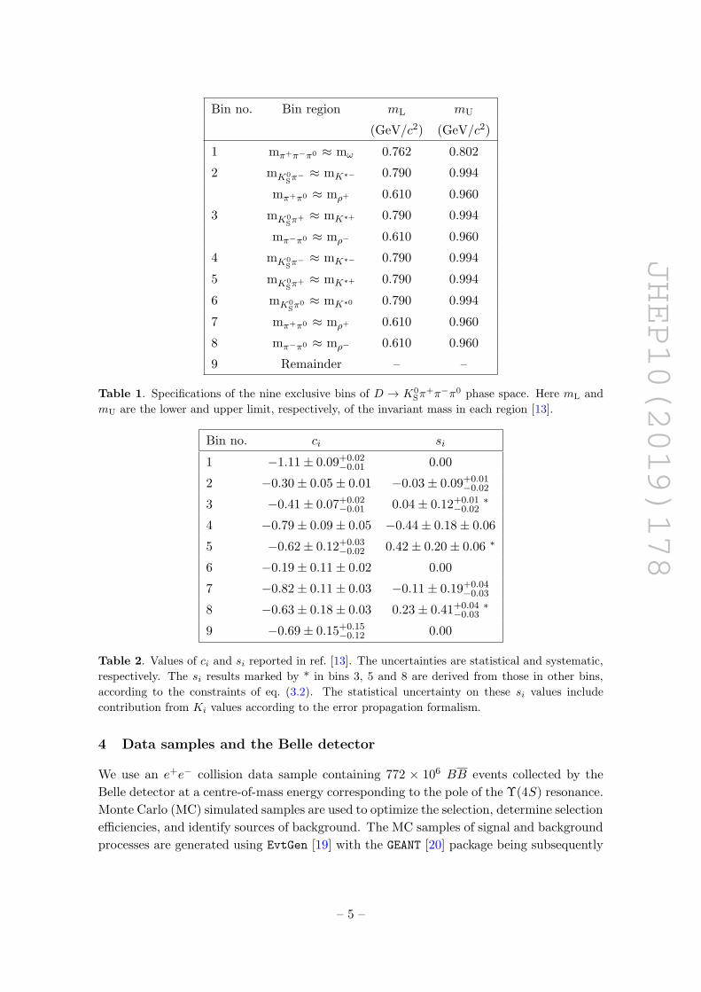
where i = 2, 4 and 7. The results for ci and si are summarized in table 2 and are shown

in figure 1. In the analysis we use the same binning scheme so that ci and si can be taken

as external inputs in determining x± and y±.

– 4 –

JHEP10(2019)178

Bin no. Bin region mL mU

(GeV/c2) (GeV/c2)

1 mπ+π−π0 ≈ mω 0.762 0.802

2 mK0Sπ

− ≈ mK∗− 0.790 0.994

mπ+π0 ≈ mρ+ 0.610 0.960

3 mK0Sπ

+ ≈ mK∗+ 0.790 0.994

mπ−π0 ≈ mρ− 0.610 0.960

4 mK0Sπ

− ≈ mK∗− 0.790 0.994

5 mK0Sπ

+ ≈ mK∗+ 0.790 0.994

6 mK0Sπ

0 ≈ mK∗0 0.790 0.994

7 mπ+π0 ≈ mρ+ 0.610 0.960

8 mπ−π0 ≈ mρ− 0.610 0.960

9 Remainder – –

Table 1. Specifications of the nine exclusive bins of D → K0Sπ

+π−π0 phase space. Here mL and

mU are the lower and upper limit, respectively, of the invariant mass in each region [13].

Bin no. ci si

1 −1.11± 0.09+0.02−0.01 0.00

2 −0.30± 0.05± 0.01 −0.03± 0.09+0.01−0.02

3 −0.41± 0.07+0.02−0.01 0.04± 0.12+0.01 ∗

−0.02

4 −0.79± 0.09± 0.05 −0.44± 0.18± 0.06

5 −0.62± 0.12+0.03−0.02 0.42± 0.20± 0.06 ∗

6 −0.19± 0.11± 0.02 0.00

7 −0.82± 0.11± 0.03 −0.11± 0.19+0.04−0.03

8 −0.63± 0.18± 0.03 0.23± 0.41+0.04 ∗−0.03

9 −0.69± 0.15+0.15−0.12 0.00

Table 2. Values of ci and si reported in ref. [13]. The uncertainties are statistical and systematic,

respectively. The si results marked by * in bins 3, 5 and 8 are derived from those in other bins,

according to the constraints of eq. (3.2). The statistical uncertainty on these si values include

contribution from Ki values according to the error propagation formalism.

4 Data samples and the Belle detector

We use an e+e− collision data sample containing 772 × 106 BB events collected by the

Belle detector at a centre-of-mass energy corresponding to the pole of the Υ(4S) resonance.

Monte Carlo (MC) simulated samples are used to optimize the selection, determine selection

efficiencies, and identify sources of background. The MC samples of signal and background

processes are generated using EvtGen [19] with the GEANT [20] package being subsequently

– 5 –

JHEP10(2019)178

ic

-1.5 -1 -0.5 0 0.5 1 1.5

is

-1.5

-1

-0.5

0

0.5

1

1.5

1 69

2

3

4

7

8

5

Figure 1. Values of ci and si reported in ref. [13]. The black and red error bars represent statistical

and systematic uncertainties, respectively.

used to model the detector response to the decay products. PHOTOS [21] incorporates effects

due to final-state radiation from charged particles.

The Belle detector [22, 23] was located at the interaction point of the KEKB

asymmetric-energy e+e− collider [24, 25]. The detector subsystems relevant for this study

are: the silicon vertex detector (SVD) and central drift chamber (CDC), for charged particle

tracking and measurement of energy loss due to ionization (dE/dx); the aerogel thresh-

old Cherenkov counters (ACC) and time-of-flight (TOF) scintillation counters, for particle

identification (PID); and the electromagnetic calorimeter (ECL) consisting of an array of

CsI(Tl) crystals to measure photon energies. These subsystems are situated in a magnetic

field of 1.5 T. A more detailed description of the Belle detector can be found in refs. [22, 23].

5 Analysis overview

The essence of the analysis lies in eqs. (2.5) and (2.6), which describe the partial decay

rates in each bin. However, these relations do not account for experimental resolution and

acceptance. For example, the invariant mass resolution causes events to be assigned to bins

outside of their origin, an effect we shall call “migration”. The background contributions

are to be considered as well. Here we briefly summarize how these experimental effects are

accounted for.

– 6 –

JHEP10(2019)178

5.1 Efficiency

Three different samples are used in this analysis, each with differing selection efficiencies

due to the kinematic differences between the final states: the quantum correlated DD

sample from ψ(3770) decays, the Belle sample of B+ → Dh+, where h = (K,π), and the

Belle sample of D∗+ → Dπ+ used to determine Ki and Ki. The sample of B+ → Dπ+ is

used as a control sample, as it is topologically identical to the signal, but with negligible

expected CP violation [26]. The ci and si results measured with CLEO-c data have been

corrected for efficiency. Efficiency variation among bins will not matter if the efficiency

profile is the same for both B+ → Dh+ and flavour-tagged D samples. This is partially

achieved by requiring similar kinematic properties for the D meson in both samples. The

efficiency profile depends primarily on D momentum, hence we select the flavour-tagged D

sample in such a way that the D momentum approximately matches that of the B+ → Dh+

sample. The matching is not exact, so independent efficiency corrections are applied to the

yields in both samples while calculating the parameters of interest.

5.2 Momentum resolution

The finite momentum resolution causes events to migrate among the bins. The ci and siresults are obtained after applying corrections for these migration effects. The amount of

migration in both B and D∗ samples is estimated as a migration matrix Mij . The matrix

has its diagonal elements close to one, and off-diagonal elements are small. MC samples

of signal events are used to obtain the migration matrix. The data yield in each bin, Yi,

is modified as Y ′i = MijYj . Any difference between the invariant mass resolution in the

data and MC samples must be taken into account. We find the effect of the difference

in resolution is only significant in bin 1, which contains the ω resonance. This bin is

narrow due to the small natural width of the ω. However, the natural width is the same

order as the mπ+π−π0 resolution, so there is significant migration out of this bin that is

not compensated by migration into bin 1. Therefore, the M1j elements of the migration

matrix are determined after applying a Gaussian smearing to the value of mπ+π−π0 by a

scale factor. The scale factor is obtained from the observed difference in ω mass resolution

between data and MC samples. The scale factors are 1.13 ± 0.02 and 1.09 ± 0.02 for the

B+ → Dh+ and D∗+ → Dπ+ samples, respectively.

5.3 Signal extraction

It is important to account for the background contributions in the sample while extracting

the specified parameters. An extended maximum likelihood fit is performed on the data

in each bin of the flavour-tagged D sample to extract the values of Ki and Ki. The fit to

the B sample in the bins of D phase space is performed using an extended likelihood fit

that simultaneously fits all bins in the B+ → DK+ and B+ → Dπ+ decay modes, so that

the values of the parameters x± and y± that are common to the expectation for each bin

yield, can be extracted, as well as the cross-feed between these samples.

– 7 –

JHEP10(2019)178

6 Event selection

We reconstruct the decays B+ → DK+ and B+ → Dπ+, where the neutral D meson decays

to the four-body final state of K0Sπ

+π−π0. In addition, D∗+ → D0π+ decays produced via

the e+e− → cc continuum process are selected to determine the Ki and Ki parameters.

For charged particle candidates originating directly from the B and D decays, we

require that the track be within 0.5 cm and ±3.0 cm of the interaction point (IP) in the

directions perpendicular to (radial) and parallel to the z-axis, respectively; the z-axis is

defined to be opposite to the e+ beam direction. The charged tracks are classified as pions

or kaons based on information from CDC, ACC, and TOF sub-detector systems. The pion

(kaon) identification efficiency is 92% (84%) and the probability of misidentification as a

kaon (pion) is 15% (8%) [27].

We select K0S candidates from two oppositely charged tracks assumed to be pions. The

invariant mass of the two tracks is required to be within the range 0.487–0.508 GeV/c2

corresponding to ±3σ of the known K0S mass [12], where σ is the mass resolution. A neural

network [28] based selection is applied on the daughter tracks to remove background from

random combinations [29, chapter 4]. The input variables to the neural network are the K0S

momentum in the lab frame, the distance between the two track helices along the z-axis

at their point of closest approach, the K0S flight length in the radial direction, the angle

between the K0S momentum and the vector joining the IP to the K0

S decay vertex, the

angle between pion momentum and the boost direction of lab frame in K0S rest frame and

pion momentum in K0S rest frame, the distances of closest approach in the radial direction

between IP and the two pion helices, the number of hits in CDC for each pion track, and

the presence of hits in the SVD for each pion track. The K0S selection efficiency is 87%,

which is determined from an MC sample of generic BB events.

The π0 candidates are reconstructed from pairs of photons detected in the ECL. We

select candidates with diphoton invariant mass Mπ0 in the range 0.119–0.148 GeV/c2, which

corresponds to 3σ about the nominal π0 mass [12]. The photon energy thresholds are

optimized separately for π0 candidates detected in combinations of the barrel, forward

endcap (FWD EC) and backward endcap (BWD EC) regions of the ECL as given in

table 3 by maximizing the significance S/√S +B, where S and B are the number of

signal and background events selected from MC samples in the signal region, respectively.

(The criteria that define the signal region are described later in this section.) Studies of

MC samples indicate that candidates in the other ECL sector combinations make up only

1.5% of the total, and a common energy threshold of 50 MeV is applied on these. All

selected combinations of K0Sπ

+π−π0 candidates are retained for further study. In addition,

kinematic constraints are applied to the K0S, π0, and D invariant masses and decay vertices

to improve the momentum resolution of the B candidates, as well as the invariant masses

used to bin the D phase space.

The D∗+ → D0π+ decay uses the charge of the accompanying pion to identify the

flavour of the D meson. This pion is referred to as a slow pion because of the limited

phase space of the decay that results in it having lower momentum on average than other

final-state particles. To improve the momentum resolution of the slow pion, it is required

– 8 –

JHEP10(2019)178

γ1 γ2 Eγ1 (MeV) Eγ2 (MeV)

Barrel Barrel 70 65

FWD EC Barrel 220 65

Barrel BWD EC 65 95

FWD EC FWD EC 150 210

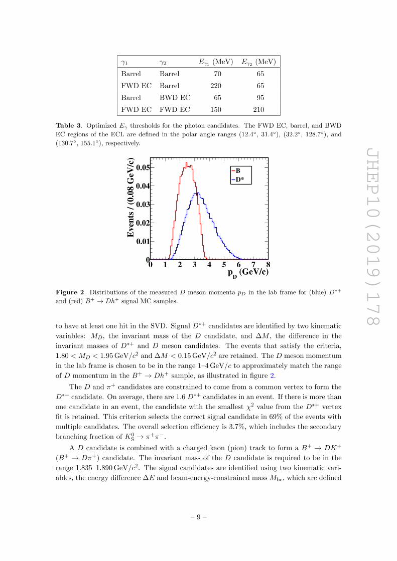
Table 3. Optimized Eγ thresholds for the photon candidates. The FWD EC, barrel, and BWD

EC regions of the ECL are defined in the polar angle ranges (12.4◦, 31.4◦), (32.2◦, 128.7◦), and

(130.7◦, 155.1◦), respectively.

(GeV/c)D

p0 1 2 3 4 5 6 7 8

Even

ts /

(0.0

8 G

eV/c

)

0

0.01

0.02

0.03

0.04

0.05 B

D*

Figure 2. Distributions of the measured D meson momenta pD in the lab frame for (blue) D∗+

and (red) B+ → Dh+ signal MC samples.

to have at least one hit in the SVD. Signal D∗+ candidates are identified by two kinematic

variables: MD, the invariant mass of the D candidate, and ∆M , the difference in the

invariant masses of D∗+ and D meson candidates. The events that satisfy the criteria,

1.80 < MD < 1.95 GeV/c2 and ∆M < 0.15 GeV/c2 are retained. The D meson momentum

in the lab frame is chosen to be in the range 1–4 GeV/c to approximately match the range

of D momentum in the B+ → Dh+ sample, as illustrated in figure 2.

The D and π+ candidates are constrained to come from a common vertex to form the

D∗+ candidate. On average, there are 1.6 D∗+ candidates in an event. If there is more than

one candidate in an event, the candidate with the smallest χ2 value from the D∗+ vertex

fit is retained. This criterion selects the correct signal candidate in 69% of the events with

multiple candidates. The overall selection efficiency is 3.7%, which includes the secondary

branching fraction of K0S → π+π−.

A D candidate is combined with a charged kaon (pion) track to form a B+ → DK+

(B+ → Dπ+) candidate. The invariant mass of the D candidate is required to be in the

range 1.835–1.890 GeV/c2. The signal candidates are identified using two kinematic vari-

ables, the energy difference ∆E and beam-energy-constrained mass Mbc, which are defined

– 9 –

JHEP10(2019)178

as ∆E = EB−Ebeam and Mbc = c−2√E2

beam − |~pB|2c2, where EB (~pB) is the energy (mo-

mentum) of the B candidate and Ebeam is the beam energy in the centre-of-mass frame. We

select candidates that satisfy the criteria Mbc > 5.27 GeV/c2 and −0.13 < ∆E < 0.30 GeV.

The asymmetric ∆E window is chosen to avoid the peaking structure appearing at lower

values from partially reconstructed B+ → D(∗)K(∗)+ decays. The signal region used while

performing optimization of the selection is |∆E| < 0.05 GeV. The average B candidate

multiplicity is 1.3. In events with more than one candidate, we retain the candidate with

the smallest value of(Mbc−MPDG

BσMbc

)2+(MD−MPDG

DσMD

)2+(Mπ0−M

PDGπ0

σMπ0

)2. Here, the masses

MPDGi are those reported by the Particle Data Group [12] and the resolutions σMbc

, σMD,

and σMπ0are obtained from MC simulated samples of signal events. The best candidate

selection criterion is 80% efficient in selecting the correctly reconstructed candidate.

The background from e+e− → qq (q = u, d, s, c) continuum processes is suppressed

by exploiting the difference in event topology compared to e+e− → Υ(4S) → BB events.

The continuum events are jet-like in nature, whereas BB events have a spherical topology,

due to the low momentum of the B mesons produced via the Υ(4S) resonance. A neural-

network-based algorithm [28] is used to discriminate between continuum background and

B events. We also use variables related to the displaced vertices of B decays from the IP

and the associated leptons/kaons from the non-signal B meson in the event, which give an

additional handle to distinguish continuum events.

The eight input variables to the neural network are the likelihood ratio obtained via

Fisher discriminants [30] formed from modified Fox-Wolfram moments [31, 32], the absolute

value of the cosine of the angle between the B candidate and the z axis in the e+e− centre-

of-mass frame, the absolute value of the cosine of the angle between the thrust axis of

the B candidate and that of the rest of the event in the centre-of-mass frame, the vertex

separation between the two B candidates [33] along z-axis, the absolute value of the B

flavour-dilution factor [34], the difference between the sum of the charges of particles in

the hemisphere about the D direction in the centre-of-mass frame and the one in the

opposite hemisphere, excluding the particles used for the reconstruction of B, the product

of the charge of the B and the sum of the charges of all kaons not used for reconstruction

of B, and the cosine of the angle between the D direction and the direction opposite to

that of the Υ(4S) in the B rest frame.

Signal and continuum MC samples are used to train the neural network. We require

the neural network output, CNN, to be greater than −0.6, which reduces the continuum

background by 67% with a loss of only 5% of the signal. The overall selection efficiency is

4.7% and 5.3% for B+ → DK+ and B+ → Dπ+ decays, respectively. These efficiencies

include the secondary branching fraction of K0S → π+π−. The efficiencies in each bin and

the migration matrix for the B+ → Dh+ selection are given in appendix A.

7 Determination of Ki and Ki from the D∗+ sample

The fractions of D0 and D0

events in each D phase space bin, represented as Ki and

Ki, are measured from the selected sample of D∗+ → Dπ+ candidates. The yield of signal

– 10 –

JHEP10(2019)178

events is obtained from a two-dimensional unbinned extended maximum-likelihood fit to the

distribution of MD and ∆M for the selected candidates. The fit is performed independently

in each bin. In general, there are two types of background: combinatorial, which is due

to the random combination of final-state particles to form a D∗+ candidate, and random-

slow-pion, in which a correctly reconstructed D meson combines with a π+, which is not

from a common D∗+ decay, to form a candidate. The combinatorial background peaks

neither in the MD nor ∆M distributions, whereas the random-slow-pion background peaks

only in the MD distribution.

The signal component of the MD distribution is described by a probability density

function (PDF) that is the sum of a Crystal Ball (CB) [35, appendix E] function and

two Gaussian functions with a common mean. The combinatorial background PDF is

parametrized by a first-order polynomial. The signal PDF is also used to model the random-

slow-pion background distribution in MD. The ∆M signal PDF is described by the sum

of an asymmetric Gaussian and three Gaussian functions with a common mean. The

combinatorial background ∆M distribution is parametrized by the sum of a threshold

function and two Gaussian PDFs. The threshold function is

f(∆M) = (∆M −mπ)12 + α(∆M −mπ)

32 + β(∆M −mπ)

52 , (7.1)

where mπ is the mass of a charged pion [12], and α and β are shape parameters. In the

final fit to data, the shape parameters are fixed to the values obtained from MC. The

Gaussian functions describe a small peak in the ∆M combinatorial distribution, which is

due to misreconstructed π0 candidates. The parameters of the Gaussian functions and the

fraction of candidates in the peak are fixed to the values obtained from a MC sample. The

random-slow-pion background PDF is the same as the threshold function used to describe

the combinatorial background.

The signal MD and ∆M PDFs are correlated such that the width of the ∆M dis-

tribution depends upon MD. The width of the core Gaussian in the ∆M signal PDF is

parametrized as

σ(∆M) = a0 + a2(MD −MPDGD )2, (7.2)

where a0 and a2 are parameters to be determined from data. The correlation between

MD and ∆M distributions is found to be negligible in studies of background MC samples.

Therefore, the one-dimensional PDFs are multiplied to obtain the total background PDF.

The yields, except that describing the peaking component in the combinatorial back-

ground ∆M distribution and the shape parameters a0(2), as well as the means of the signal

in both MD and ∆M are floated in the fit; all other parameters are fixed to the values

obtained from fits to the corresponding MC sample. In each bin, the fit is performed si-

multaneously for D0 and D0

categories to obtain the signal yield. Figure 3 shows the fit

projections compared to the data within bin 1. These projections are signal-enhanced by

considering events in the signal region of the variable that is not plotted; the signal regions

are defined as 1.86 < MD < 1.87 GeV/c2 and 0.144 < ∆M < 0.146 GeV/c2. The large

statistics of the sample makes it difficult for the model to fit data exactly, resulting in

systematic deviations in the pull values from zero in the tails. Studies of MC samples have

– 11 –

JHEP10(2019)178

)2 (GeV/cDM1.8 1.82 1.84 1.86 1.88 1.9 1.92 1.94

)2

Even

ts /

(1.5

MeV

/c

0

1

2

3

4

5

6

310×

Data

Total fit

Signal

Combinatorial

Random-slow-pion

(a)

Pu

ll

-404

)2M (GeV/c∆

0.14 0.142 0.144 0.146 0.148 0.15

)2

Ev

ents

/ (

0.1

MeV

/c

0

1

2

3

4

5

310×

Data

Total fit

Signal

Combinatorial

Random-slow-pion

(b)

Pu

ll

-404

Figure 3. Signal-enhanced fit projections of (a) MD and (b) ∆M distributions from D∗± → Dπ±

data sample in bin 1. The black points with error bars are the data and the solid blue curves

show the total fit. The error bars are barely visible as they are smaller than the size of the points.

The dotted red, blue and magenta curves represent the signal, combinatorial and random-slow-pion

backgrounds, respectively. The pull between the fit and the data is shown below the distributions.

Bin no. ND0 ND

0 Ki Ki

1 51048±282 50254±280 0.2229±0.0008 0.2249±0.0008

2 137245±535 58222±382 0.4410±0.0009 0.1871±0.0007

3 31027±297 105147±476 0.0954±0.0005 0.3481±0.0009

4 24203±280 16718±246 0.0726±0.0005 0.0478±0.0004

5 13517±220 20023±255 0.0371±0.0003 0.0611±0.0004

6 21278±269 20721±267 0.0672±0.0005 0.0679±0.0005

7 15784±221 13839±209 0.0403±0.0004 0.0394±0.0004

8 6270±148 7744±164 0.0165±0.0002 0.0183±0.0002

9 6849±193 6698±192 0.0070±0.0002 0.0054±0.0001

Table 4. D0 and D0

yield in each bin of D phase space along with Ki and Ki values measured in

D∗ tagged data sample.

shown that the signal yield is unbiased and this systematic deviation in the pull values has

negligible effect on the measured Ki and Ki values. The efficiency- and migration-corrected

yields are then used to determine the values of Ki and Ki, which are given in table 4. The

values of Ki and Ki are in reasonable agreement with those reported in ref. [13]; the only

deviation larger than 3σ is in bin 9, which contains only 1.2% of the data.

– 12 –

JHEP10(2019)178

8 Determination of (x±, y±) from the B± → Dh± sample

We select both B+ → DK+ and B+ → Dπ+ decays because they have an identical topol-

ogy, but the latter is less sensitive to CP -violation measurements because rDπB is approxi-

mately twenty times smaller than rDKB . However, the B+ → Dπ+ branching fraction is an

order of magnitude larger than that of B+ → DK+ and hence serves as an excellent cali-

bration sample for the signal determination procedure. Furthermore, there is a significant

background from B+ → Dπ+ decays in the B+ → DK+ sample from the misidentification

of the charged pion as a kaon; a simultaneous fit to both samples allows this cross-feed to

be directly determined from data.

The signal yield in each bin is obtained via a simultaneous two-dimensional fit to the

nine D phase space bins with the data divided into B+ → DK+, B− → DK−, B+ → Dπ+

and B− → Dπ− candidates, so there are 36 samples in total. The signal extraction is done

by fitting ∆E and CNN. The distribution of CNN cannot be described readily by an analytic

PDF. Therefore, we transform CNN as

C ′NN = log

(CNN − CNN,low

CNN,high − CNN

), (8.1)

where CNN,low = −0.6 and CNN,high = 0.9985 are the minimum and maximum values of

CNN in the sample, respectively. The signal and background distributions of C ′NN can be

described by combinations of Gaussian PDFs. The three background components consid-

ered are:

• continuum background from e+e− → qq processes, where q = (u, d, s, c)

• combinatorial BB background, in which the final state particles could be coming

from both B mesons in an event; and

• cross-feed peaking background from B+ → Dh+, where h = π, K, in which the

charged kaon is misidentified as a pion or vice versa.

There is no significant correlation between ∆E and C ′NN, so the two-dimensional PDF

for each of the components is the product of one-dimensional ∆E and C ′NN PDFs. The

sum of a CB function and two Gaussian functions with a common mean is used as the

PDF to model the ∆E signal component in both B samples. The sum of a Gaussian and

an asymmetric Gaussian with different mean values is used to parametrize the PDF that

describes the C ′NN signal component. The continuum background distribution is modeled

with a first-order polynomial in ∆E and by the sum of two Gaussian PDFs with different

mean values in C ′NN. The ∆E distribution of combinatorial BB background in B+ → Dπ+

is described by an exponential function. There is a small peaking structure due to misre-

constructed π0 events, and this is modeled by a CB function. A first-order polynomial is

added to the above two PDFs in the case of B+ → DK+ decays. The C ′NN distribution

for each of the samples is modeled by an asymmetric Gaussian function. The cross-feed

peaking background in ∆E is modeled with the sum of three Gaussian functions, whereas

the signal PDF itself is used for the C ′NN distribution.

– 13 –

JHEP10(2019)178

E (GeV)∆

-0.1 0 0.1 0.2 0.3

Even

ts /

(8.6

MeV

)

0

100

200

300Data

Total fit

Signal

qContinuum q

BCombinatorial B

cross-feedπK-

(a)P

ull

-4

0

4NNC'

-10 -5 0 5 10

Even

ts /

(0.4

8)

0

50

100

150Data

Total fit

Signal

qContinuum q

BCombinatorial B

cross-feedπK-

(b)

Pu

ll-4

0

4

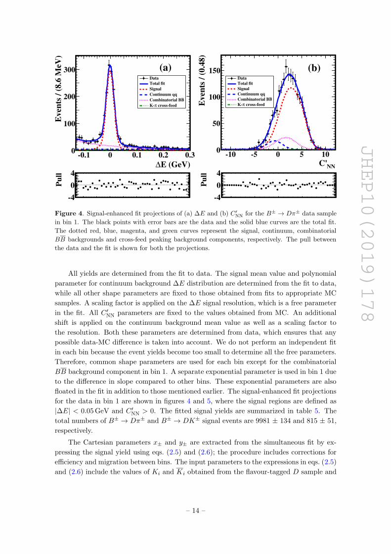
Figure 4. Signal-enhanced fit projections of (a) ∆E and (b) C ′NN for the B± → Dπ± data sample

in bin 1. The black points with error bars are the data and the solid blue curves are the total fit.

The dotted red, blue, magenta, and green curves represent the signal, continuum, combinatorial

BB backgrounds and cross-feed peaking background components, respectively. The pull between

the data and the fit is shown for both the projections.

All yields are determined from the fit to data. The signal mean value and polynomial

parameter for continuum background ∆E distribution are determined from the fit to data,

while all other shape parameters are fixed to those obtained from fits to appropriate MC

samples. A scaling factor is applied on the ∆E signal resolution, which is a free parameter

in the fit. All C ′NN parameters are fixed to the values obtained from MC. An additional

shift is applied on the continuum background mean value as well as a scaling factor to

the resolution. Both these parameters are determined from data, which ensures that any

possible data-MC difference is taken into account. We do not perform an independent fit

in each bin because the event yields become too small to determine all the free parameters.

Therefore, common shape parameters are used for each bin except for the combinatorial

BB background component in bin 1. A separate exponential parameter is used in bin 1 due

to the difference in slope compared to other bins. These exponential parameters are also

floated in the fit in addition to those mentioned earlier. The signal-enhanced fit projections

for the data in bin 1 are shown in figures 4 and 5, where the signal regions are defined as

|∆E| < 0.05 GeV and C ′NN > 0. The fitted signal yields are summarized in table 5. The

total numbers of B± → Dπ± and B± → DK± signal events are 9981 ± 134 and 815 ± 51,

respectively.

The Cartesian parameters x± and y± are extracted from the simultaneous fit by ex-

pressing the signal yield using eqs. (2.5) and (2.6); the procedure includes corrections for

efficiency and migration between bins. The input parameters to the expressions in eqs. (2.5)

and (2.6) include the values of Ki and Ki obtained from the flavour-tagged D sample and

– 14 –

JHEP10(2019)178

E (GeV)∆

-0.1 0 0.1 0.2 0.3

Even

ts /

(8.6

MeV

)

0

10

20

30Data

Total fit

Signal

qContinuum q

BCombinatorial B

cross-feedπK-

(a)P

ull

-4

0

4NNC'

-10 -5 0 5 10

Even

ts /

(0.4

8)

0

10

20

30

40Data

Total fit

Signal

qContinuum q

BCombinatorial B

cross-feedπK-

(b)

Pu

ll-4

0

4

Figure 5. Signal-enhanced fit projections of (a) ∆E and (b) C ′NN for the B± → DK± data sample

in bin 1. The black points with error bars are the data and the solid blue curves are the total fit.

The dotted red, blue, magenta, and green curves represent the signal, continuum, combinatorial

BB backgrounds and cross-feed peaking background components, respectively. The pull between

the data and the fit is also shown for both the projections.

B± → Dπ± B± → DK±

Bin no. N+i N−i N+

i N−i

1 772±33 860±34 80±13 58±12

2 1077±41 2088±55 98±16 190±21

3 1639±49 450±28 121±18 57±13

4 263±24 451±29 21±9 30±11

5 377±27 256±23 23±9 18±9

6 338±26 321±26 35±11 23±9

7 253±21 255±22 16±9 5±7

8 154±17 109±15 9±6 13±7

9 162±19 138±19 21±9 30±10

Table 5. Signal yields in each D phase space bin for B± → Dπ± and B± → DK± data samples

obtained from a simultaneous fit to the nine bins.

the D strong-phase difference parameters ci and si [13]. The results are summarized in

table 6, and the statistical likelihood contours are shown in figure 6. The statistical cor-

relation matrices are given in tables 7 and 8. The measured and expected yields for the

binned B+ and B− data are compared in figures 7 and 8.

– 15 –

JHEP10(2019)178

B± → Dπ± B± → DK±

x+ 0.039 ± 0.024 +0.018 +0.014−0.013 −0.012 −0.030 ± 0.121 +0.017 +0.019

−0.018 −0.018

y+ −0.196 +0.080 +0.038 +0.032−0.059 −0.034 −0.030 0.220 +0.182

−0.541 ± 0.032 +0.072−0.071

x− −0.014 ±0.021 +0.018 +0.019−0.010 −0.010 0.095 ± 0.121 +0.017 +0.023

−0.016 −0.025

y− −0.033 ± 0.059+0.018 +0.019−0.019 −0.010 0.354 +0.144 +0.015 +0.032

−0.197 −0.021 −0.049

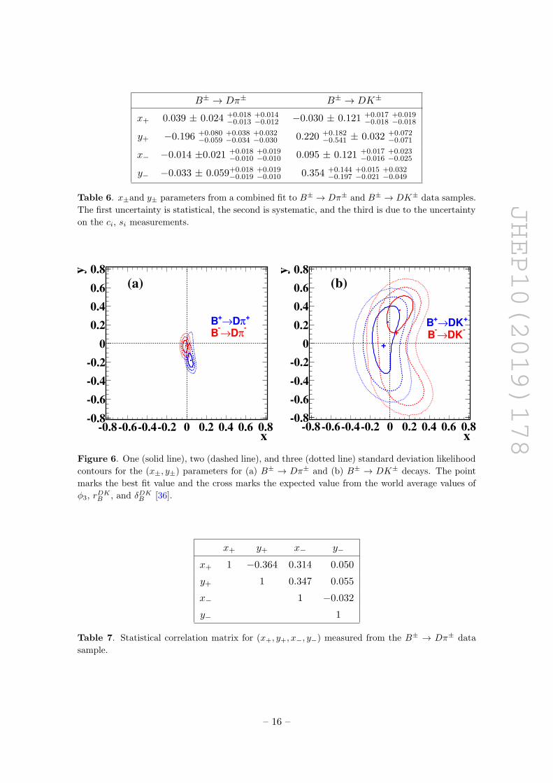
Table 6. x±and y± parameters from a combined fit to B± → Dπ± and B± → DK± data samples.

The first uncertainty is statistical, the second is systematic, and the third is due to the uncertainty

on the ci, si measurements.

x-0.8-0.6-0.4-0.2 0 0.2 0.4 0.6 0.8

y

-0.8

-0.6

-0.4

-0.2

0

0.2

0.4

0.6

0.8

.

.

+πD→

+B

-πD→

-B

(a)

x-0.8-0.6-0.4-0.2 0 0.2 0.4 0.6 0.8

y

-0.8

-0.6

-0.4

-0.2

0

0.2

0.4

0.6

0.8

.

.

+

+

+DK→

+B

-DK→

-B

(b)

Figure 6. One (solid line), two (dashed line), and three (dotted line) standard deviation likelihood

contours for the (x±, y±) parameters for (a) B± → Dπ± and (b) B± → DK± decays. The point

marks the best fit value and the cross marks the expected value from the world average values of

φ3, rDKB , and δDKB [36].

x+ y+ x− y−

x+ 1 −0.364 0.314 0.050

y+ 1 0.347 0.055

x− 1 −0.032

y− 1

Table 7. Statistical correlation matrix for (x+, y+, x−, y−) measured from the B± → Dπ± data

sample.

– 16 –

JHEP10(2019)178

Bin number1 2 3 4 5 6 7 8 9

πD+

N

0

0.5

1

1.5

2

310×

(best fit x, y)predM

measM

(a)

Pu

ll

-5

0

5Bin number

1 2 3 4 5 6 7 8 9

πD-

N

0

0.5

1

1.5

2

310×

(best fit x, y)predM

measM

(b)

Pu

ll-5

0

5

Figure 7. Measured and expected yields in bins for (a) B+ → Dπ+ and (b) B− → Dπ− data

samples. The data points with error bars are the measured yields, and the solid histogram is the

expected yield from the best fit (x±, y±) parameter values.

Bin number1 2 3 4 5 6 7 8 9

DK

+N

0

0.05

0.1

0.15

0.2

310×

(best fit x, y)predM

measM

(a)

Pu

ll

-5

0

5Bin number

1 2 3 4 5 6 7 8 9

DK

-N

0

0.05

0.1

0.15

0.2

310×

(best fit x, y)predM

measM

(b)

Pu

ll

-5

0

5

Figure 8. Measured and expected yields in bins for (a) B+ → DK+ and (b) B− → DK− data

samples. The data points with error bars are the measured yields, and the solid histogram is the

expected yield from the best fit (x±, y±) parameter values.

– 17 –

JHEP10(2019)178

x+ y+ x− y−

x+ 1 0.486 0.172 −0.231

y+ 1 −0.127 0.179

x− 1 0.365

y− 1

Table 8. Statistical correlation matrix for (x+, y+, x−, y−) measured from the B± → DK± data

sample.

9 Systematic uncertainties

We consider several possible sources of systematic uncertainty, as listed in table 9, along

with their contributions. The remainder of this section describes how these uncertainties

are estimated.

The limited size of the signal MC sample used for estimating the efficiency and the

migration matrix is a source of systematic uncertainty. Efficiencies in B and D∗ samples

are varied by their statistical uncertainty (±1σ) in each bin independently. The resultant

negative and positive deviations in (x±, y±) are separately summed in quadrature. Sim-

ilarly, the migration matrix elements are varied by their statistical uncertainty in B and

D∗ samples, one element at a time. The resultant positive and negative deviations are

considered separately.

The systematic uncertainty due to the difference in mass resolution between data and

the MC samples is considered by varying the width on the π+π−π0 invariant mass distribu-

tion by the uncertainty on the resolution scale factor obtained in data, when compared to

that in MC. The resultant deviations in (x±, y±) are taken as the systematic uncertainty

from this source. All the other resonances are wide and the resolution difference is an order

of magnitude smaller than the resolution, thus the modelling of resolution does not affect

our measurements. The systematic effect of the uncertainty on the Ki and Ki values is

estimated by varying them by their statistical uncertainties independently. The resultant

sum of deviations in quadrature is taken as the associated systematic uncertainty.

Modelling the data with PDFs that have parameters fixed to values obtained from MC

samples is another source of systematic uncertainty. There are 14 signal and 23 background

shape parameters fixed in the B± → Dh± simultaneous fit. These are fixed to the values

obtained from MC samples. The uncertainty due to PDF modelling is taken into account

by repeating the fit by individually varying the fixed parameters by ±1σ, where σ is

the uncertainty on these parameters in MC component fits, and taking the difference in

quadrature as the uncertainty. Any possible bias in the fit is studied with a set of pseudo-

experiments with different input values for (x±, y±). The fit is found to give an unbiased

response within the statistical uncertainty from the finite number of pseudo-experiments,

and this uncertainty is taken as the systematic uncertainty from this source.

The kaon identification efficiency and pion fake rate used in the fit are also fixed

parameters that are determined from control samples of D∗+ → D0π+, D0 → K−π+. They

– 18 –

JHEP10(2019)178

Source B± → Dπ± B± → DK±

x+ y+ x− y− x+ y+ x− y−

Efficiency +0.013 +0.030 +0.012 +0.012 +0.012 +0.022 +0.012 +0.013

uncertainty −0.009 −0.027 −0.008 −0.013 −0.013 −0.023 −0.012 −0.016

Migration matrix +0.011 +0.021 +0.011 +0.013 +0.007 +0.015 +0.007 +0.006

uncertainty −0.004 −0.019 −0.003 −0.014 −0.008 −0.016 −0.007 −0.012

mπππ0 resolution 0.003 0.001 0.004 0.001 0.001 0.001 0.001 0.003

Ki, Ki +0.004 +0.007 +0.004 +0.002 +0.001 +0.001 +0.002 +0.001

uncertainty −0.001 −0.006 −0.001 −0.002 −0.002 −0.001 −0.002 −0.001

PDF shape +0.004 +0.004 +0.004 +0.001 +0.009 +0.017 +0.009 +0.001

−0.008 −0.003 −0.004 −0.001 −0.008 −0.016 −0.007 −0.005

Fit bias 0.000 0.001 0.000 0.000 0.001 0.001 0.001 0.003

PID 0.001 0.001 0.001 0.000 0.002 0.001 0.002 0.001

Total systematic +0.018 +0.038 +0.018 +0.018 +0.017 +0.032 +0.017 +0.015

uncertainty −0.013 −0.034 −0.010 −0.019 −0.018 −0.032 −0.016 −0.021

ci, si +0.014 +0.032 +0.010 +0.019 +0.019 +0.072 +0.023 +0.032

uncertainty −0.012 −0.030 −0.006 −0.010 −0.018 −0.071 −0.025 −0.049

Total statistical +0.024 +0.080 +0.021 +0.059 +0.121 +0.182 +0.121 +0.144

uncertainty −0.024 −0.059 −0.021 −0.059 −0.121 −0.541 −0.121 −0.197

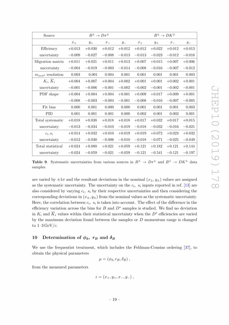
Table 9. Systematic uncertainties from various sources in B± → Dπ± and B± → DK± data

samples.

are varied by ±1σ and the resultant deviations in the nominal (x±, y±) values are assigned

as the systematic uncertainty. The uncertainty on the ci, si inputs reported in ref. [13] are

also considered by varying ci, si by their respective uncertainties and then considering the

corresponding deviations in (x±, y±) from the nominal values as the systematic uncertainty.

Here, the correlation between ci, si is taken into account. The effect of the difference in the

efficiency variation across the bins for B and D∗ samples is studied. We find no deviation

in Ki and Ki values within their statistical uncertainty when the D∗ efficiencies are varied

by the maximum deviation found between the samples or D momentum range is changed

to 1–3 GeV/c.

10 Determination of φ3, rB and δB

We use the frequentist treatment, which includes the Feldman-Cousins ordering [37], to

obtain the physical parameters

µ = (φ3, rB, δB) ,

from the measured parameters

z = (x+, y+, x−, y−) ,

– 19 –

JHEP10(2019)178

Parameter Results 2σ interval

φ3 (◦) 5.7 +10.2−8.8 ± 3.5 ± 5.7 (−29.7, 109.5)

δB (◦) 83.4 +18.3−16.6 ± 3.1 ± 4.0 (35.7, 175.0)

rB 0.323 ± 0.147 ± 0.023 ± 0.051 (0.031, 0.616)

Table 10. (φ3, δB , rB) obtained from the B± → DK± data sample. The first uncertainty is

statistical, second is systematic and, the third one is due to the uncertainty on ci, si measurements.

in B± → DK± sample; this is the same procedure as was used in ref. [11]. We do not

use the B± → Dπ± sample to constrain φ3, which has been the case in previous Belle

analyses [11, 38]. We note that the constraints presented by the LHCb Collaboration [39]

allow values up to rDπB < 0.028 at a 2σ confidence level, which is five times larger than the

expectation; if the value of rDπB is significantly larger than expected then future analyses

could include B± → Dπ± channel to determine φ3. The confidence level is calculated as

α(µ) =

∫D(µ) p(z|µ)dz∫∞ p(z|µ)dz

, (10.1)

where p(z|µ) is the probability density to observe the measurements z given the set of

physical parameters µ. The integration domain D(µ) is given by the likelihood ratio or-

dering in the Feldman-Cousins method. The PDF p(z|µ) is a multivariate Gaussian PDF

with the uncertainties and correlations between (x±, y±) taken from the measurements.

We obtain the parameters µ = (φ3, rB, δB) from the fit as given in table 10. The

systematic uncertainty is estimated by varying the z parameters by their corresponding

systematic uncertainties. Figure 9 shows the confidence level contours representing one,

two, and three standard deviations in (φ3, rB) and (φ3, δB) planes.

We performed a check of the assumption that the (x±, y±) likelihood can be approx-

imated to be Gaussian when using the Feldman-Cousins method to extract (φ3, rB, δB).

The check used the measured confidence intervals in (φ3, rB, δB) to generate an ensemble of

simulated data sets. Each simulated data set was then fit to form a distribution of (x±, y±),

which was found to be consistent with the (x±, y±) confidence intervals measured. Hence

we conclude that the reported confidence intervals for (φ3, rB, δB) are appropriate.

There is a two-fold ambiguity in φ3 and δB results with φ3 + 180◦ and δB + 180◦.

We choose the solution that satisfies 0◦ < φ3 < 180◦. This result includes the current

world-average value [36] within two standard deviations. We observe that there is a local

minimum of the likelihood around φ3 = 75◦ and δB = 155◦.

We combine the results presented here with the model-independent

B+→D(K0Sπ

+π−)K+ [11] and B0→D0(K0Sπ

+π−)K∗0 [38] results from Belle. Without

our measurement, the combination leads to φ3 = (78+14−15)◦. Including our measurement,

the combination gives φ3 = (74+13−14)◦. The distributions of p-values for the φ3 measure-

ments from the individual D final states and the combination are given in figure 10. The

separate measurements and the combination likelihood contours in the (φ3, rB) plane are

shown in figure 11.

– 20 –

JHEP10(2019)178

(degrees)3

φ0 50 100 150 200 250 300 350

Br

0

0.1

0.2

0.3

0.4

0.5

0.6

0.7

0.8

0.9

1

. .

(a)

+ +

(degrees)3

φ0 50 100 150 200 250 300 350

(d

egre

es)

Bδ

0

50

100

150

200

250

300

350

.

.

(b)

+

+

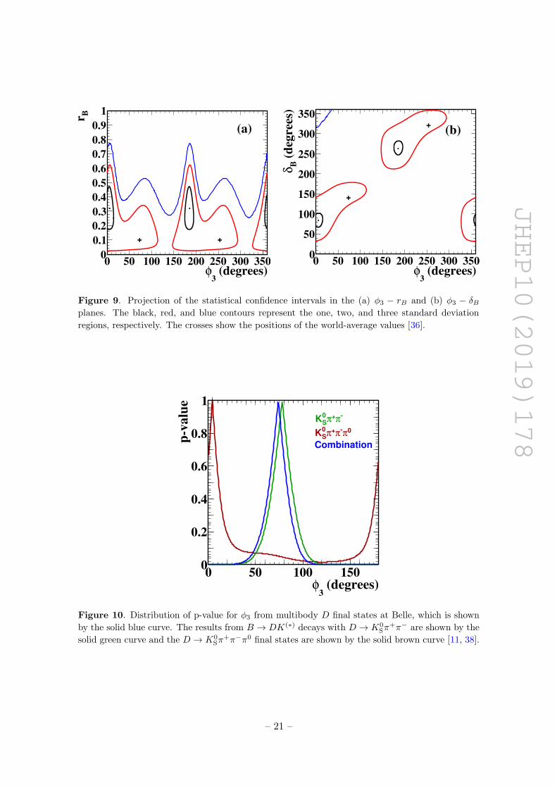
Figure 9. Projection of the statistical confidence intervals in the (a) φ3 − rB and (b) φ3 − δBplanes. The black, red, and blue contours represent the one, two, and three standard deviation

regions, respectively. The crosses show the positions of the world-average values [36].

(degrees)3

φ0 50 100 150

p-v

alu

e

0

0.2

0.4

0.6

0.8

1-π+π

0

SK

0π-π+π0

SK

Combination

Figure 10. Distribution of p-value for φ3 from multibody D final states at Belle, which is shown

by the solid blue curve. The results from B → DK(∗) decays with D → K0Sπ

+π− are shown by the

solid green curve and the D → K0Sπ

+π−π0 final states are shown by the solid brown curve [11, 38].

– 21 –

JHEP10(2019)178

(degrees)3

φ0 50 100 150

Br

0

0.1

0.2

0.3

0.4-π+π

0

SK

0π-π+π0

SK

Combination

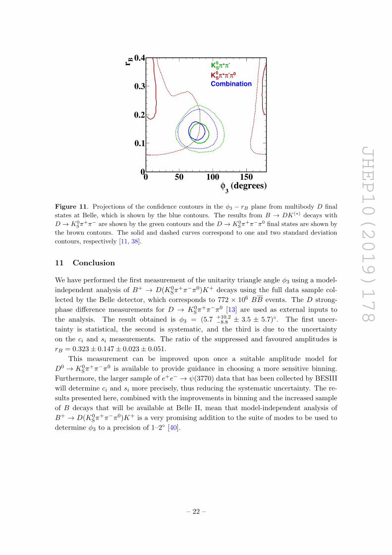
Figure 11. Projections of the confidence contours in the φ3 − rB plane from multibody D final

states at Belle, which is shown by the blue contours. The results from B → DK(∗) decays with

D → K0Sπ

+π− are shown by the green contours and the D → K0Sπ

+π−π0 final states are shown by

the brown contours. The solid and dashed curves correspond to one and two standard deviation

contours, respectively [11, 38].

11 Conclusion

We have performed the first measurement of the unitarity triangle angle φ3 using a model-

independent analysis of B+ → D(K0Sπ

+π−π0)K+ decays using the full data sample col-

lected by the Belle detector, which corresponds to 772 × 106 BB events. The D strong-

phase difference measurements for D → K0Sπ

+π−π0 [13] are used as external inputs to

the analysis. The result obtained is φ3 = (5.7 +10.2−8.8 ± 3.5 ± 5.7)◦. The first uncer-

tainty is statistical, the second is systematic, and the third is due to the uncertainty

on the ci and si measurements. The ratio of the suppressed and favoured amplitudes is

rB = 0.323± 0.147± 0.023± 0.051.

This measurement can be improved upon once a suitable amplitude model for

D0 → K0Sπ

+π−π0 is available to provide guidance in choosing a more sensitive binning.

Furthermore, the larger sample of e+e− → ψ(3770) data that has been collected by BESIII

will determine ci and si more precisely, thus reducing the systematic uncertainty. The re-

sults presented here, combined with the improvements in binning and the increased sample

of B decays that will be available at Belle II, mean that model-independent analysis of

B+ → D(K0Sπ

+π−π0)K+ is a very promising addition to the suite of modes to be used to

determine φ3 to a precision of 1–2◦ [40].

– 22 –

JHEP10(2019)178

Acknowledgments

We thank the KEKB group for the excellent operation of the accelerator; the KEK cryo-

genics group for the efficient operation of the solenoid; and the KEK computer group,

and the Pacific Northwest National Laboratory (PNNL) Environmental Molecular Sci-

ences Laboratory (EMSL) computing group for strong computing support; and the Na-

tional Institute of Informatics, and Science Information NETwork 5 (SINET5) for valu-

able network support. We acknowledge support from the Ministry of Education, Culture,

Sports, Science, and Technology (MEXT) of Japan, the Japan Society for the Promotion

of Science (JSPS), and the Tau-Lepton Physics Research Center of Nagoya University; the

Australian Research Council including grants DP180102629, DP170102389, DP170102204,

DP150103061, FT130100303; Austrian Science Fund (FWF); the National Natural Sci-

ence Foundation of China under Contracts No. 11435013, No. 11475187, No. 11521505,

No. 11575017, No. 11675166, No. 11705209; Key Research Program of Frontier Sciences,

Chinese Academy of Sciences (CAS), Grant No. QYZDJ-SSW-SLH011; the CAS Center

for Excellence in Particle Physics (CCEPP); the Shanghai Pujiang Program under Grant

No. 18PJ1401000; the Ministry of Education, Youth and Sports of the Czech Republic

under Contract No. LTT17020; the Carl Zeiss Foundation, the Deutsche Forschungsge-

meinschaft, the Excellence Cluster Universe, and the VolkswagenStiftung; the Depart-

ment of Science and Technology of India; the Istituto Nazionale di Fisica Nucleare of

Italy; National Research Foundation (NRF) of Korea Grants No. 2016R1D1A1B01010135,

No. 2016R1D1A1B02012900, No. 2018R1A2B3003643, No. 2018R1A6A1A06024970,

No. 2018R1D1A1B07047294, No. 2019K1A3A7A09033840; Radiation Science Research In-

stitute, Foreign Large-size Research Facility Application Supporting project, the Global

Science Experimental Data Hub Center of the Korea Institute of Science and Technol-

ogy Information and KREONET/GLORIAD; the Polish Ministry of Science and Higher

Education and the National Science Center; the Grant of the Russian Federation Govern-

ment, Agreement No. 14.W03.31.0026; the Slovenian Research Agency; Ikerbasque, Basque

Foundation for Science, Spain; the Swiss National Science Foundation; the Ministry of Ed-

ucation and the Ministry of Science and Technology of Taiwan; and the United States

Department of Energy and the National Science Foundation.

– 23 –

JHEP10(2019)178

A Efficiency and migration matrix

The efficiencies in nine bins of D phase space in D∗± → Dπ±, B± → DK± and B± → Dπ±

decays determined from signal MC samples are given in table 11. The migration matrices

for B+ → DK+ and B+ → Dπ+ decays estimated from signal MC samples are given in

tables 12 and 13, respectively.

Bin ε (%)

D∗+ → D0π+ D∗− → D0π− B+ → DK+ B− → DK− B+ → Dπ+ B− → Dπ−

1 3.07±0.06 3.02±0.06 3.77±0.05 3.84±0.05 4.43±0.06 4.35±0.06

2 3.77±0.05 4.83±0.09 5.44±0.07 5.01±0.04 6.15±0.08 5.47±0.04

3 5.66±0.14 3.66±0.05 4.97±0.04 4.88±0.10 5.55±0.05 5.55±0.10

4 3.60±0.11 3.72±0.12 4.55±0.10 4.63±0.09 5.29±0.11 5.17±0.09

5 3.77±0.14 3.38±0.11 4.89±0.10 4.28±0.10 5.47±0.10 4.53±0.11

6 3.71±0.11 3.45±0.11 4.68±0.09 4.28±0.09 5.46±0.10 5.04±0.09

7 3.87±0.17 4.03±0.19 4.92±0.16 4.66±0.14 5.64±0.18 5.29±0.14

8 3.36±0.24 3.53±0.21 5.36±0.19 4.77±0.20 5.75±0.20 5.56±0.22

9 3.32±0.16 3.21±0.16 4.64±0.14 4.21±0.13 4.87±0.15 4.83±0.14

Table 11. Efficiency in each bin of the D phase space for D∗± → Dπ±, B± → DK±, and

B± → Dπ± decays determined from the corresponding signal MC samples.

Bin no. 1 2 3 4 5 6 7 8 9

1 0.93 0.01 0.01 0.01 0.01 0.01 0.00 0.00 0.01

2 0.01 0.96 0.02 0.00 0.00 0.00 0.00 0.00 0.00

3 0.01 0.02 0.95 0.00 0.00 0.00 0.00 0.00 0.00

4 0.04 0.03 0.02 0.90 0.00 0.00 0.00 0.00 0.01

5 0.04 0.01 0.03 0.01 0.91 0.01 0.00 0.00 0.01

6 0.02 0.02 0.01 0.01 0.01 0.92 0.01 0.00 0.00

7 0.01 0.03 0.02 0.00 0.01 0.02 0.91 0.00 0.01

8 0.01 0.02 0.02 0.01 0.00 0.01 0.01 0.88 0.02

9 0.06 0.02 0.02 0.01 0.01 0.01 0.01 0.00 0.86

Table 12. Migration matrix for B+ → DK+ decays estimated from the signal MC sample. The

rows correspond to the true bins and columns show the reconstructed bins.

– 24 –

JHEP10(2019)178

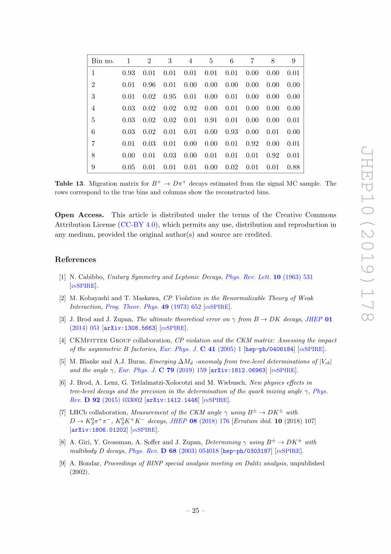
Bin no. 1 2 3 4 5 6 7 8 9

1 0.93 0.01 0.01 0.01 0.01 0.01 0.00 0.00 0.01

2 0.01 0.96 0.01 0.00 0.00 0.00 0.00 0.00 0.00

3 0.01 0.02 0.95 0.01 0.00 0.01 0.00 0.00 0.00

4 0.03 0.02 0.02 0.92 0.00 0.01 0.00 0.00 0.00

5 0.03 0.02 0.02 0.01 0.91 0.01 0.00 0.00 0.01

6 0.03 0.02 0.01 0.01 0.00 0.93 0.00 0.01 0.00

7 0.01 0.03 0.01 0.00 0.00 0.01 0.92 0.00 0.01

8 0.00 0.01 0.03 0.00 0.01 0.01 0.01 0.92 0.01

9 0.05 0.01 0.01 0.01 0.00 0.02 0.01 0.01 0.88

Table 13. Migration matrix for B+ → Dπ+ decays estimated from the signal MC sample. The

rows correspond to the true bins and columns show the reconstructed bins.

Open Access. This article is distributed under the terms of the Creative Commons

Attribution License (CC-BY 4.0), which permits any use, distribution and reproduction in

any medium, provided the original author(s) and source are credited.

References

[1] N. Cabibbo, Unitary Symmetry and Leptonic Decays, Phys. Rev. Lett. 10 (1963) 531

[INSPIRE].

[2] M. Kobayashi and T. Maskawa, CP Violation in the Renormalizable Theory of Weak

Interaction, Prog. Theor. Phys. 49 (1973) 652 [INSPIRE].

[3] J. Brod and J. Zupan, The ultimate theoretical error on γ from B → DK decays, JHEP 01

(2014) 051 [arXiv:1308.5663] [INSPIRE].

[4] CKMfitter Group collaboration, CP violation and the CKM matrix: Assessing the impact

of the asymmetric B factories, Eur. Phys. J. C 41 (2005) 1 [hep-ph/0406184] [INSPIRE].

[5] M. Blanke and A.J. Buras, Emerging ∆Md -anomaly from tree-level determinations of |Vcb|and the angle γ, Eur. Phys. J. C 79 (2019) 159 [arXiv:1812.06963] [INSPIRE].

[6] J. Brod, A. Lenz, G. Tetlalmatzi-Xolocotzi and M. Wiebusch, New physics effects in

tree-level decays and the precision in the determination of the quark mixing angle γ, Phys.

Rev. D 92 (2015) 033002 [arXiv:1412.1446] [INSPIRE].

[7] LHCb collaboration, Measurement of the CKM angle γ using B± → DK± with

D → K0Sπ

+π−, K0SK

+K− decays, JHEP 08 (2018) 176 [Erratum ibid. 10 (2018) 107]

[arXiv:1806.01202] [INSPIRE].

[8] A. Giri, Y. Grossman, A. Soffer and J. Zupan, Determining γ using B± → DK± with

multibody D decays, Phys. Rev. D 68 (2003) 054018 [hep-ph/0303187] [INSPIRE].

[9] A. Bondar, Proceedings of BINP special analysis meeting on Dalitz analysis, unpublished

(2002).

– 25 –

JHEP10(2019)178

[10] CLEO collaboration, Model-independent determination of the strong-phase difference

between D0 and D0 → K0S,Lh

+h− (h = π,K) and its impact on the measurement of the

CKM angle γ/φ3, Phys. Rev. D 82 (2010) 112006 [arXiv:1010.2817] [INSPIRE].

[11] Belle collaboration, First measurement of φ3 with a model-independent Dalitz plot analysis

of B± → DK±, D → K0Sπ

+π− decay, Phys. Rev. D 85 (2012) 112014 [arXiv:1204.6561]

[INSPIRE].

[12] Particle Data Group, Review of Particle Physics, Phys. Rev. D 98 (2018) 030001

[INSPIRE].

[13] P.K. Resmi, J. Libby, S. Malde and G. Wilkinson, Quantum-correlated measurements of

D → K0Sπ

+π−π0 decays and consequences for the determination of the CKM angle γ, JHEP

01 (2018) 082 [arXiv:1710.10086] [INSPIRE].

[14] CLEO collaboration, The CLEO-II detector, Nucl. Instrum. Meth. A 320 (1992) 66

[INSPIRE].

[15] D. Peterson et al., The CLEO III drift chamber, Nucl. Instrum. Meth. A 478 (2002) 142

[INSPIRE].

[16] M. Artuso et al., Construction, pattern recognition and performance of the CLEO-III

LiF-TEA RICH detector, Nucl. Instrum. Meth. A 502 (2003) 91 [hep-ex/0209009]

[INSPIRE].

[17] CLEO-c/CESR-c taskforces and CLEO-c collaboration, CLEO-c and CESR-c: a new

frontier of weak and strong interactions, Cornell LEPP Report CLNS Report No. 01/1742

(2001) [INSPIRE].

[18] Belle collaboration, Evidence for direct CP violation in the decay B± → D(∗)K±,

D → K0Sπ

+π− and measurement of the CKM phase φ3, Phys. Rev. D 81 (2010) 112002

[arXiv:1003.3360] [INSPIRE].

[19] D.J. Lange, The EvtGen particle decay simulation package, Nucl. Instrum. Meth. A 462

(2001) 152 [INSPIRE].

[20] R. Brun et al., GEANT 3.21, CERN Program Library Long Writeup W5013, unpublished.

[21] E. Barberio and Z. Was, PHOTOS: A Universal Monte Carlo for QED radiative corrections.

Version 2.0, Comput. Phys. Commun. 79 (1994) 291 [INSPIRE].

[22] Belle collaboration, The Belle Detector, Nucl. Instrum. Meth. A 479 (2002) 117 [INSPIRE].

[23] Belle collaboration, Physics Achievements from the Belle Experiment, PTEP 2012 (2012)

04D001 [arXiv:1212.5342] [INSPIRE].

[24] S. Kurokawa and E. Kikutani, Overview of the KEKB accelerators, Nucl. Instrum. Meth. A

499 (2003) 1 [INSPIRE].

[25] T. Abe et al., Achievements of KEKB, PTEP 2013 (2013) 03A001 [INSPIRE].

[26] M. Kenzie, M. Martinelli and N. Tuning, Estimating rDπB as an input to the determination of

the CKM angle γ, Phys. Rev. D 94 (2016) 054021 [arXiv:1606.09129] [INSPIRE].

[27] Belle collaboration, Evidence for the Suppressed Decay B− → DK−, D → K+π−, Phys.

Rev. Lett. 106 (2011) 231803 [arXiv:1103.5951] [INSPIRE].

[28] M. Feindt and U. Kerzel, The NeuroBayes neural network package, Nucl. Instrum. Meth. A

559 (2006) 190 [INSPIRE].

– 26 –

JHEP10(2019)178

[29] H. Nakano, Search for new physics by a time-dependent CP violation analysis of the decay

B → KSηγ using the Belle detector, Ph.D. Thesis, Tohoku University (2014)

[https://belle.kek.jp/belle/theses/doctor/nakano15.pdf].

[30] R.A. Fisher, The use of multiple measurements in taxonomic problems, Annals Eugen. 7

(1936) 179 [INSPIRE].

[31] G.C. Fox and S. Wolfram, Observables for the Analysis of Event Shapes in e+e−

Annihilation and Other Processes, Phys. Rev. Lett. 41 (1978) 1581 [INSPIRE].

[32] Belle collaboration, Evidence for B0 → π0π0, Phys. Rev. Lett. 91 (2003) 261801

[hep-ex/0308040] [INSPIRE].

[33] H. Tajima et al., Proper time resolution function for measurement of time evolution of B

mesons at the KEK B factory, Nucl. Instrum. Meth. A 533 (2004) 370 [hep-ex/0301026]

[INSPIRE].

[34] Belle collaboration, Neutral B flavor tagging for the measurement of mixing induced

CP-violation at Belle, Nucl. Instrum. Meth. A 533 (2004) 516 [hep-ex/0403022] [INSPIRE].

[35] T. Skwarnicki, A study of the radiative cascade transitions between the Υ and Υ′ resonances,

Ph.D. Thesis, DESY F31-86-02 (1986).

[36] HFLAV collaboration, Averages of b-hadron, c-hadron and τ -lepton properties as of summer

2016, Eur. Phys. J. C 77 (2017) 895 [arXiv:1612.07233] [INSPIRE].

[37] G.J. Feldman and R.D. Cousins, A Unified approach to the classical statistical analysis of

small signals, Phys. Rev. D 57 (1998) 3873 [physics/9711021] [INSPIRE].

[38] Belle collaboration, First model-independent Dalitz analysis of B0 → DK∗0, D → K0Sπ

+π−

decay, PTEP 2016 (2016) 043C01 [arXiv:1509.01098] [INSPIRE].

[39] LHCb collaboration, Measurement of the CKM angle γ from a combination of LHCb results,

JHEP 12 (2016) 087 [arXiv:1611.03076] [INSPIRE].

[40] Belle-II collaboration, The Belle II Physics Book, arXiv:1808.10567 [INSPIRE].

– 27 –