Published for SISSA by Springer2014...JHEP07(2014)072 Published for SISSA by Springer Received: May...
21
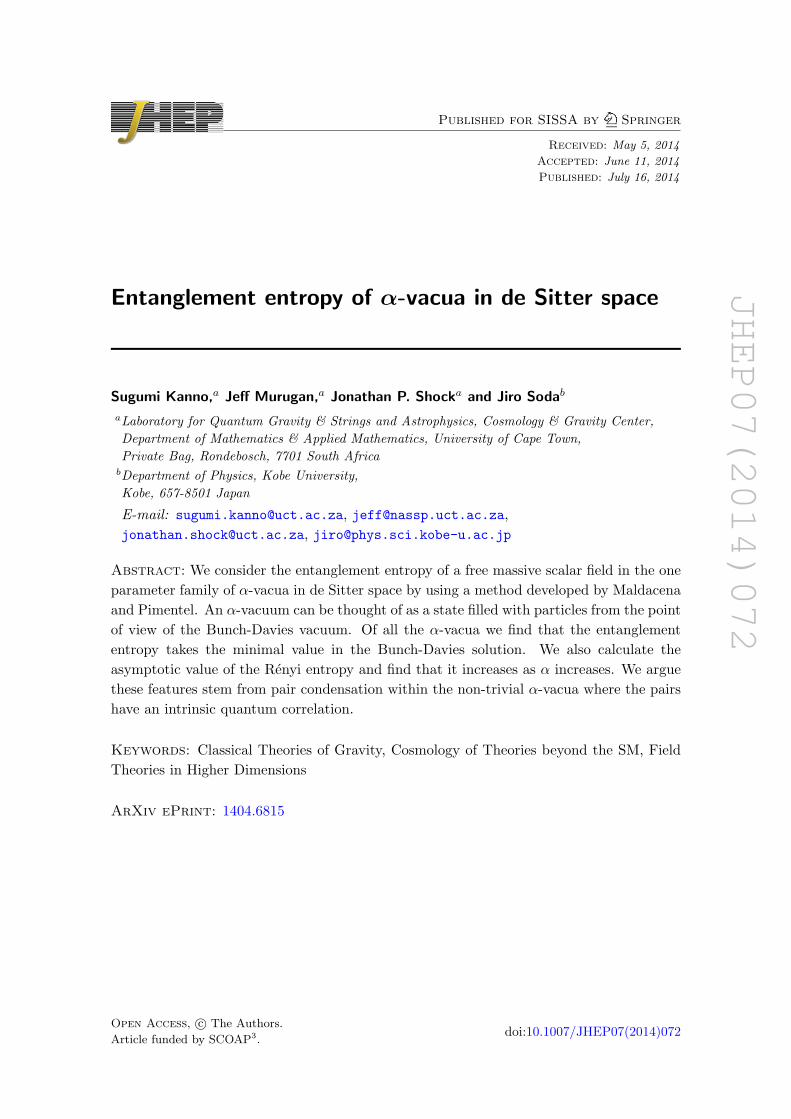
JHEP07(2014)072 Published for SISSA by Springer Received: May 5, 2014 Accepted: June 11, 2014 Published: July 16, 2014 Entanglement entropy of α-vacua in de Sitter space Sugumi Kanno, a Jeff Murugan, a Jonathan P. Shock a and Jiro Soda b a Laboratory for Quantum Gravity & Strings and Astrophysics, Cosmology & Gravity Center, Department of Mathematics & Applied Mathematics, University of Cape Town, Private Bag, Rondebosch, 7701 South Africa b Department of Physics, Kobe University, Kobe, 657-8501 Japan E-mail: [email protected], [email protected], [email protected], [email protected] Abstract: We consider the entanglement entropy of a free massive scalar field in the one parameter family of α-vacua in de Sitter space by using a method developed by Maldacena and Pimentel. An α-vacuum can be thought of as a state filled with particles from the point of view of the Bunch-Davies vacuum. Of all the α-vacua we find that the entanglement entropy takes the minimal value in the Bunch-Davies solution. We also calculate the asymptotic value of the R´ enyi entropy and find that it increases as α increases. We argue these features stem from pair condensation within the non-trivial α-vacua where the pairs have an intrinsic quantum correlation. Keywords: Classical Theories of Gravity, Cosmology of Theories beyond the SM, Field Theories in Higher Dimensions ArXiv ePrint: 1404.6815 Open Access,c The Authors. Article funded by SCOAP 3 . doi:10.1007/JHEP07(2014)072
Transcript of Published for SISSA by Springer2014...JHEP07(2014)072 Published for SISSA by Springer Received: May...
JHEP07(2014)072
Published for SISSA by Springer
Received: May 5, 2014
Accepted: June 11, 2014
Published: July 16, 2014
Entanglement entropy of α-vacua in de Sitter space
Sugumi Kanno,a Jeff Murugan,a Jonathan P. Shocka and Jiro Sodab
aLaboratory for Quantum Gravity & Strings and Astrophysics, Cosmology & Gravity Center,
Department of Mathematics & Applied Mathematics, University of Cape Town,
Private Bag, Rondebosch, 7701 South AfricabDepartment of Physics, Kobe University,
Kobe, 657-8501 Japan
E-mail: [email protected], [email protected],
[email protected], [email protected]
Abstract: We consider the entanglement entropy of a free massive scalar field in the one
parameter family of α-vacua in de Sitter space by using a method developed by Maldacena
and Pimentel. An α-vacuum can be thought of as a state filled with particles from the point
of view of the Bunch-Davies vacuum. Of all the α-vacua we find that the entanglement
entropy takes the minimal value in the Bunch-Davies solution. We also calculate the
asymptotic value of the Renyi entropy and find that it increases as α increases. We argue
these features stem from pair condensation within the non-trivial α-vacua where the pairs
have an intrinsic quantum correlation.
Keywords: Classical Theories of Gravity, Cosmology of Theories beyond the SM, Field
Theories in Higher Dimensions
ArXiv ePrint: 1404.6815
Open Access, c© The Authors.
Article funded by SCOAP3.doi:10.1007/JHEP07(2014)072
JHEP07(2014)072
Contents
1 Introduction 1
2 A review of entanglement entropy of the Bunch-Davies vacuum 3
2.1 Entanglement entropy 3
2.2 Setup of entanglement entropy in de Sitter space 4
2.3 Entanglement entropy in the Bunch-Davies vacuum 5
2.4 Large mass range 10
2.5 Super-curvature modes 11
3 Entanglement entropy of α-vacua 11
3.1 α-vacua 11
3.2 Bogoliubov transformation to R, L-vacua 12
3.3 Diagonalization 13
3.4 Long range entanglement entropy 14
3.5 Large mass range 15
3.6 Renyi entropy 15
4 Discussion 17
1 Introduction
It is well recognized that entanglement entropy is a useful tool to characterize a quan-
tum state [1]. Historically, quantum entanglement has been one of the most mysterious
and fascinating features of quantum mechanics in that performing a local measurement
may instantaneously affect the outcome of local measurements beyond the lightcone. This
apparent violation of causality is known as the Einstein-Podolsky-Rosen paradox [2]. How-
ever, since information does not get transferred in such a measurement, causality remains
intact. There are many phenomena which we are now finding that quantum entanglement
may play a role, including bubble nucleation [3]. Schwinger pair production in a constant
electric field can be considered as an analogue of bubble nucleation in a false vacuum. In
the case of pair creation, electron-positron pairs are spontaneously created with a certain
separation and such particle states should then be quantum correlated. Recent studies of
the Schwinger effect infer that observer frames will be strongly correlated to each other
when they observe the nucleation frame [4–6].
Entanglement entropy has now been established as a suitable measure of the degree of
entanglement of a quantum system. Entanglement entropy has since become a useful tool
in understanding phenomena in condensed matter physics, quantum information and high
energy physics. For example, entanglement entropy plays the roll of an order parameter
– 1 –
JHEP07(2014)072
in condensed matter systems and thus the phase structure can be examined using this
measure of quantum correlation. It would be interesting to consider the consequences of a
measurable entanglement entropy in a cosmological setting, especially in view of the bubble
nucleation and the multiverse. Indeed, it may be possible to investigate whether a universe
entangled with our own universe exists within the multiverse framework. Such a scenario
may be observable through the cosmic microwave background radiation (CMB).
To calculate the entanglement entropy in quantum field theories explicitly has, until
recently, not been an easy task. In [7], Ryu and Takayanagi proposed a method of calcu-
lating the entanglement entropy of a strongly coupled quantum field theory with a gravity
dual using holographic techniques. This has proved extremely powerful and their formula
has passed many consistency checks [8]. Consequently, entanglement entropy, especially
within a holographic context has been attracting a great deal of attention of late.
In [9] Maldacena and Pimentel developed a method to explicitly calculate the entan-
glement entropy in a quantum field theory in the Bunch-Davies vacuum of de Sitter space
and discussed the gravitational dual of this theory and its holographic interpretation. In
this paper, we extend the calculation of the entanglement entropy in the Bunch-Davies vac-
uum to α-vacua. The use of conformal symmetry of the de Sitter invariant Bunch-Davies
vacuum as utilized by Maldacena and Pimental can be also extended to the α-vacua and
this will significantly simplify the calculation.
Our interest in α-vacua is three-fold: firstly, these new examples serve to further
develop our understanding of the nature of entanglement entropy in the non-trivial vacua
with de Sitter invariance. Second, understanding entanglement entropy in this de Sitter
invariant family of backgrounds will provide a non-trivial check of the holographic methods
employed by Ryu and Takayanagi which even today is the only tool at our disposal to
access the entanglement entropy of strongly-coupled quantum field theories. We would like
to clarify here how the change of the vacuum can be implemented into the holographic
scheme. This is related to the issue of how to describe the entanglement entropy of excited
states from the holographic point of view. Our final motivation stems from cosmology.
In conjunction with CMB observations, it has been suggested [10] that non-Bunch-Davies
vacua are preferable to explain the results of BICEP2 [11].
In this paper we calculate the entanglement entropy of a massive scalar field in the
family of α-vacua in a fixed de Sitter background. Note that this is not the entropy of the
metric on the de Sitter horizon which has already been discussed extensively in the liter-
ature [12, 13]. Intuitively, an α-vacuum can be thought of as a state of pair condensation
or, alternatively, as a squeezed state [14–17]. Thus the quantum uncertainty of the state
is heavily constrained. The pair condensation itself has an intrinsic quantum correlation
associated with it. When the rate of pair condensation increases, it is expected that the
quantum correlation would increase. Hence, we expect an increase of the entanglement en-
tropy with increasing α parameter, corresponding to the increased pair condensation. We
are also able to investigate the Renyi entropy using the same mathematical techniques. This
will gives rise to a new measure of quantum correlation in these vacua and we will explore
the α dependence. We try to give a holographic interpretation in the discussion, however,
we find it difficult to implement the change of the vacuum in a conventional manner.
– 2 –

JHEP07(2014)072
The paper is organized as follows. In section 2, we review the method developed
by Maldacena and Pimentel with some comments relevant to the calculation of the en-
tanglement entropy of α-vacua. In section 3, we introduce the α-vacua and calculate the
relevant density matrix and the entanglement entropy. We also evaluate the Renyi entropy.
We conclude in section 4 with some summary remarks and speculation about a possible
holographic interpretation of our results.
2 A review of entanglement entropy of the Bunch-Davies vacuum
In [9], Maldacena and Pimentel developed a method to calculate a specific contribution
to the entanglement entropy of a massive scalar field in de Sitter space explicitly. They
showed that the long range correlations implied by the entanglement entropy are maximal
for small masses and decay exponentially as the mass increases. Here we will review the
formalism developed in that paper before extending it to α-vacua in section 3.
2.1 Entanglement entropy
The entanglement entropy is a quantity which characterizes quantum correlations of a
system. In particular it is the long-range correlations in which we will be interested. It can
be thought of as a measure of how much we can discover about the full state of a system,
given only a subsystem of it to measure. To explain this, let us divide the system into two
subsystems A and B. The Hilbert space becomes a direct product H = HA ⊗HB. As an
illustration, we choose a special state
|Ψ〉 =∑i
ci| i 〉A| i 〉B , (2.1)
where ci is the amplitude of finding the i-th state. In this case, the density matrix is
ρ = |Ψ〉〈Ψ| =∑i
∑j
cic∗j | i 〉A| i 〉B A〈 j |B〈 j | . (2.2)
If we trace over the degrees of freedom of B, we find that the density matrix of the
subsystem A is given by
ρA = TrB ρ =∑i,j,k
cic∗j B〈 k| i 〉A| i 〉B A〈 j |B〈 j | k 〉B =
∑k
|ck|2 | k 〉AA〈 k | , (2.3)
and the density matrix is normalized to 1 because of the conservation of probability
TrA ρA =∑k
|ck|2 = 1 . (2.4)
However, TrA ρ2A =
∑k |ck|4 6= 1 in general.
The entanglement entropy is defined via the density matrix as the Von-Neumann en-
tropy
S = −TrA ρA log ρA = −∑k
|ck|2 log |ck|2 , (2.5)
– 3 –
JHEP07(2014)072
where we traced over the subsystem A. For a pure state such as c1 = 1, c2 = c3 =
· · · cN = 0, the entanglement entropy is given by S = 0. For a mixed state such as
c1 = c2 = · · · cN = 1/√N , where N is the dimensionality of the correlated Hilbert space,
the entanglement entropy takes the maximum value
S = −N∑k
1
Nlog
1
N= logN . (2.6)
Since the number N describes the extent to which the system correlates, the entanglement
entropy is certainly a measure of the quantum correlations. In other words, the entangle-
ment entropy is related to the relevant degrees of freedom in the system. For instance, in
a two dimensional conformal field theory the entanglement entropy is proportional to the
central charge which counts the degrees of freedom in such a system [18].
2.2 Setup of entanglement entropy in de Sitter space
In order to study entanglement entropy in 3 + 1-dimensional de Sitter space we consider a
closed surface S2 in a hypersurface at fixed time. This divides the spacelike hypersurface
into an inside region (A) and an outside region (B). The total Hilbert space, as in the
previous section can then be written as a direct product H = Hin⊗Hout. From this we can
trace over the outside region to construct the density matrix for the internal region ρin =
Trout |Ψ〉〈Ψ|. From this we can then obtain the entanglement entropy defined in eq. (2.5).
In order to apply this procedure to de Sitter space, we first consider the closed surface
in the flat chart. In the flat chart of de Sitter space, the metric reads
ds2 =1
H2η2
[−dη2 + δij dx
idxj], (2.7)
where indices (i, j) denote the three spatial components. H is the Hubble parameter and
η is conformal time.
We consider a free scalar field of mass m on a η = constant hypersurface. The entan-
glement entropy associated to this field in the field theory consists of UV divergent and
UV finite parts
S = SUV-div + SUV-fin . (2.8)
The divergent part is well known and takes the form [19, 20]
SUV-div = c1Aε2
+ log(εH)[c2 + c3Am2 + c4AH2
], (2.9)
where ci are numerical coefficients. Here, ε is the UV-cutoff and A is the proper area of
the shared surface of the two regions. Since all of these terms arise in flat space and from
local effects, we are not interested in this part. The UV-finite part contains information
about the long-range correlations of the quantum state in de Sitter space. We can expect
the IR behavior (η → 0 limit) of the UV-finite part to be of the form
SUV-fin = c5AH2 − c6
2log(AH2
)+ finite = c5
Aη2
+ c6 log η + finite , (2.10)
– 4 –
JHEP07(2014)072
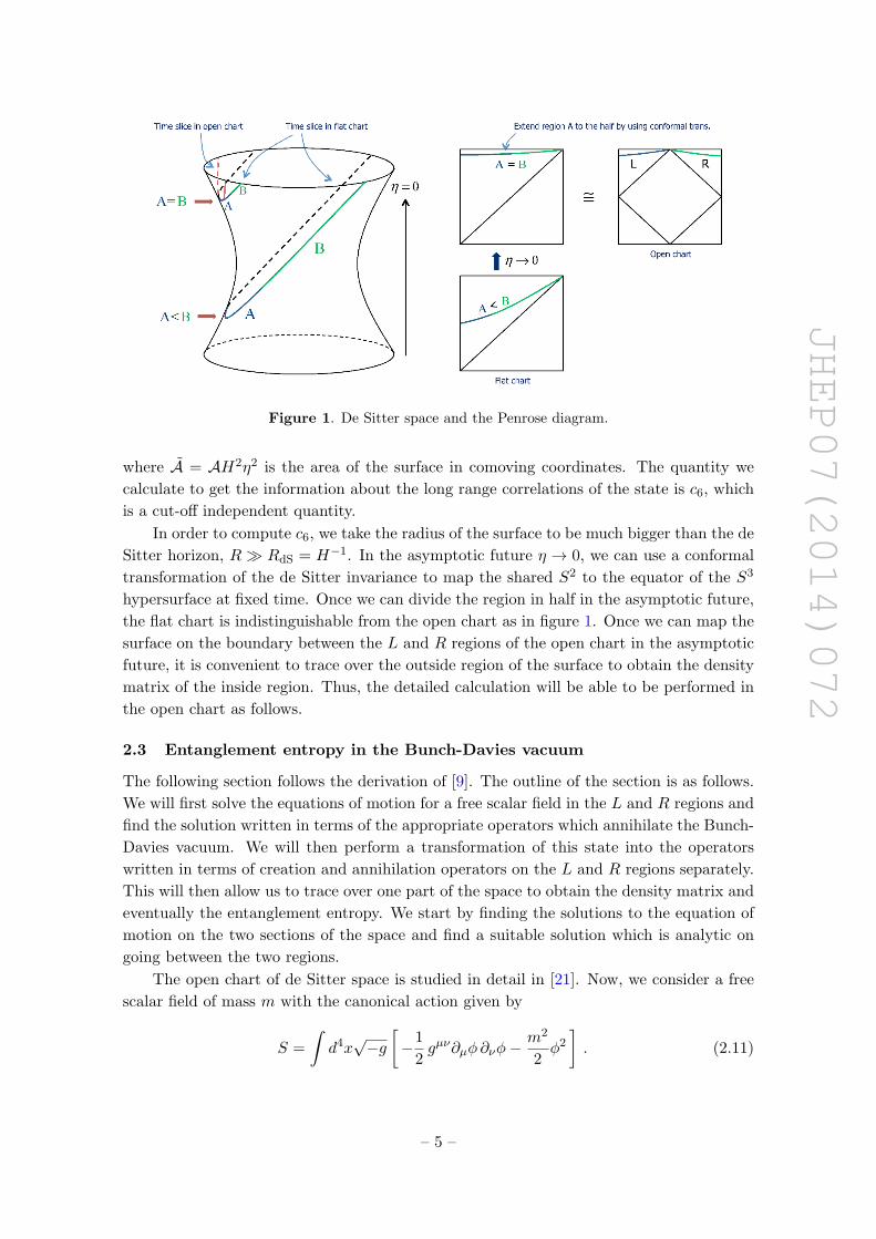
Figure 1. De Sitter space and the Penrose diagram.
where A = AH2η2 is the area of the surface in comoving coordinates. The quantity we
calculate to get the information about the long range correlations of the state is c6, which
is a cut-off independent quantity.
In order to compute c6, we take the radius of the surface to be much bigger than the de
Sitter horizon, R RdS = H−1. In the asymptotic future η → 0, we can use a conformal
transformation of the de Sitter invariance to map the shared S2 to the equator of the S3
hypersurface at fixed time. Once we can divide the region in half in the asymptotic future,
the flat chart is indistinguishable from the open chart as in figure 1. Once we can map the
surface on the boundary between the L and R regions of the open chart in the asymptotic
future, it is convenient to trace over the outside region of the surface to obtain the density
matrix of the inside region. Thus, the detailed calculation will be able to be performed in
the open chart as follows.
2.3 Entanglement entropy in the Bunch-Davies vacuum
The following section follows the derivation of [9]. The outline of the section is as follows.
We will first solve the equations of motion for a free scalar field in the L and R regions and
find the solution written in terms of the appropriate operators which annihilate the Bunch-
Davies vacuum. We will then perform a transformation of this state into the operators
written in terms of creation and annihilation operators on the L and R regions separately.
This will then allow us to trace over one part of the space to obtain the density matrix and
eventually the entanglement entropy. We start by finding the solutions to the equation of
motion on the two sections of the space and find a suitable solution which is analytic on
going between the two regions.
The open chart of de Sitter space is studied in detail in [21]. Now, we consider a free
scalar field of mass m with the canonical action given by
S =
∫d4x√−g[−1
2gµν∂µφ∂νφ−
m2
2φ2
]. (2.11)
– 5 –
JHEP07(2014)072
We write the metric in each region R and L in terms of the local definitions of t and r as
defined from the Euclidean coordinates
ds2R = H−2
[−dt2R + sinh2 tR
(dr2R + sinh2 rR dΩ2
)],
ds2L = H−2
[−dt2L + sinh2 tL
(dr2L + sinh2 rL dΩ2
)], (2.12)
where dΩ2 is the metric on the two-sphere. These coordinate systems are obtained by
analytic continuation from the Euclidean metric. Since it is natural to choose the Eu-
clidean vacuum (the Bunch-Davies vacuum [22–24]) as the initial condition, we need to
find the positive frequency mode functions corresponding to the Euclidean vacuum. After
separation of variables
φ =H
sinh tχp(t)Yp`m(r,Ω) , (2.13)
the equations of motion for χp and Yp`m in the R or L regions are found to be[∂2
∂t2+ 3 coth t
∂
∂t+
1 + p2
sinh2 t+m2
H2
]χp(t) = 0 , (2.14)[
∂2
∂r2+ 2 coth r
∂
∂r− 1
sinh2 rL2
]Yp`m(r,Ω) = −
(1 + p2
)Yp`m(r,Ω) , (2.15)
where L2 is the Laplacian operator on the unit two-sphere, the Yp`m are eigenfunctions
on the three-dimensional hyperboloid and the temporal and radial coordinates are left
undistinguished for the R and L regions. The solutions can be found explicitly in [21]. By
defining a parameter
ν =
√9
4− m2
H2, (2.16)
the time dependent part of χp(t) is given by
χp,σ(t) =
1
2 sinhπp
(eπp−iσe−iπνΓ(ν+ip+1/2)P
ipν−1/2(cosh tR)− e−πp−iσe−iπν
Γ(ν−ip+1/2) P−ipν−1/2(cosh tR)
),
σ2 sinhπp
(eπp−iσe−iπνΓ(ν+ip+1/2)P
ipν−1/2(cosh tL)− e−πp−iσe−iπν
Γ(ν−ip+1/2) P−ipν−1/2(cosh tL)
),
(2.17)
where the index σ takes the values ±1 and P±ipν− 1
2
are Legendre functions. This is a solution
supported on the R and L regions respectively. Two independent solutions for each region
are distinguished by the sign of σ. Note that the solutions are obtained by analytic contin-
uation between the L and R regions. This procedure requires the solutions to be analytic in
the Euclidean hemisphere and produces the factor e−πp in the above solutions. In this way,
the Bunch-Davies vacuum is selected. As the Bunch-Davies vacuum is de Sitter invariant,
it is legitimate to use the mapping in figure 1.
We expand the field in terms of the creation and anihilation operators,
φ(t, r,Ω) =∑σ,`,m
∫dp[aσp`m uσp`m(t, r,Ω) + a†σp`m u
∗σp`m(t, r,Ω)
], (2.18)
– 6 –
JHEP07(2014)072
where aσp`m satisfies aσp`m|BD〉 = 0. The mode function uσp`m(t, r,Ω) representing the
Bunch-Davies vacuum is
uσp`m =H
sinh tχp,σ(t)Yp`m(r,Ω) . (2.19)
In order to calculate the density matrix, we write the states in a matrix form. If we write
the bases of the L and R regions in a simple form PR,L ≡ P ipν−1/2(cosh tR,L) , P ∗R,L ≡P−ipν−1/2(cosh tR,L), the two lines of eq. (2.17) are expressed in one line
χσ = N−1p
∑q=R,L
[ασq P
q + βσq P∗ q ] , (2.20)
where the support of the functions of tL and tR are the relevant sub-regions. Np is a
normalization factor including the 1/ sinhπp in eq. (2.17) and
ασR =eπp − iσe−iπν
Γ(ν + ip+ 1
2
) , βσR = −e−πp − iσe−iπν
Γ(ν − ip+ 1
2
) , (2.21)
ασL = σeπp − iσe−iπν
Γ(ν + ip+ 1
2
) , βσL = −σ e−πp − iσe−iπν
Γ(ν − ip+ 1
2
) . (2.22)
The complex conjugate of eq. (2.20) which is needed in eq. (2.18) is
χ∗σ = N−1p
∑q=R,L
[β∗qσ P q + α∗q
σ P ∗ q ] . (2.23)
Then eq. (2.17) and its conjugate can be accommodated into the simple matrix form
χI = N−1p M I
J PJ , (2.24)
where the capital indices (I, J) run from 1 to 4 and
χI = (χσ, χ∗σ ) , M IJ =
ασq βσq
β∗qσ α∗q
σ
, P J =(PR, PL, P ∗R, P ∗L
). (2.25)
Now we focus on the time dependent part1 of the field operator, which is written as
φ(t) = aI χI = N−1
p aIMIJ P
J , aI =(aσ , a
†σ
), (2.26)
where the mode functions are defined via the appropriate annihilation of the Bunch-Davies
vacuum. Note that this relation can be regarded as the Bogoliubov transformation by
changing the mode functions defined in the Bunch-Davies vacuum into the Legendre func-
tions, which realize the positive frequency modes in the past. The Bogoliubov coefficients
are then expressed by α and β in the matrix M . To trace out the region R (or L) in the
end to obtain the density matrix of the L (or R) regions, we need to know the relation
between the Bunch-Davies vacuum and the R and L-vacua. By introducing new creation
1We omit the factor 1/ sinh t because it will be canceled when comparing eqs. (2.26) with (2.27).
– 7 –
JHEP07(2014)072
and anihilation operators bJ defined such that bR|R〉 = 0 and bL|L〉 = 0, we expand the
field operator as
φ(t) = N−1p bJ P
J , bJ =(bR , bL , b
†R , b
†L
). (2.27)
Note that we took the Legendre functions as the mode functions of the R,L-vacua because
they realize the positive frequency mode in the past. By comparing eqs. (2.26) with (2.27),
we find the relation between aJ and bJ such as
aJ = bI(M−1
)IJ ,
(M−1
)IJ =
ξqσ δqσ
δ∗qσ ξ∗qσ
,
ξ =(α− β α∗−1β∗
)−1,
δ = −α−1β ξ∗ .(2.28)
This leads to the relation between aσ and bq
aσ =∑q=R,L
[ξqσ bq + δ∗qσ b
†q
]. (2.29)
Thus, the Bunch-Davies vacuum can be regarded as the Bogoliubov transformation
from the R,L-vacua as
|BD〉 = exp
1
2
∑i,j=R,L
mij b†i b†j
|R〉|L〉 , (2.30)
where the operators bi satisfy the commutation relation[bi, b
†j
]= δij . The condition
aσ|BD〉 = 0 gives
mij = −δ∗iσ(ξ−1)σj
= −Γ (ν − ip+ 1/2)
Γ (ν + ip+ 1/2)
2 eiπν
e2πp + e2iπν
(cosπν i sinh pπ
i sinh pπ cosπν
). (2.31)
The phase terms are unimportant for ν2 > 0. We will comment on the case ν2 < 0 later in
section 2.4. Here, we consider ν2 > 0 and write them as eiθ for simplicity. Then
mij = eiθ√
2 e−pπ√cosh 2πp+ cos 2πν
(cosπν i sinh pπ
i sinh pπ cosπν
), (2.32)
where eiθ contains all phase factors. We write mRR = mLL ≡ ω, which is real and
mLR = mRL ≡ ζ, which is purely imaginary for positive ν2.
It is still difficult to trace over the R (or L) degrees of freedom when the state is
written in the form of eq. (2.30). Thus, we perform the Bogoliubov transformation again
by introducing new operators cR and cL
cR = u bR + v b†R , cL = u bL + v b†L , (2.33)
to get the relation
|BD〉 = exp(γp c
†R c†L
)|R′〉|L′〉 , (2.34)
– 8 –
JHEP07(2014)072
where |u|2−|v|2 = 1 and |u|2−|v|2 = 1 are assumed. The operators satisfy the commutation
relation[ci, c
†j
]= δij . It should be noted that the Bogoliubov transformation does not mix
L and R Hilbert spaces although the vacuum is changed by this transformation from |R〉|L〉into |R′〉|L′〉. The consistency conditions for eq. (2.34) are
cR |BD〉 = γp c†L |BD〉 , cL |BD〉 = γp c
†R |BD〉 . (2.35)
Putting eqs. (2.33) and (2.34) into eq. (2.35), we find the system of four homogeneous
equations
ω u+ v − γp ζ v∗ = 0 , ζ u− γp u∗ − γp ω v∗ = 0 , (2.36)
ω u+ v − γp ζ v∗ = 0 , ζ u− γp u∗ − γp ω v∗ = 0 . (2.37)
Here, ω is real ω∗ = ω and ζ is pure imaginary ζ∗ = −ζ for positive ν2. Taking the compex
conjugate of eq. (2.36), we find that we can set v∗ = v and u∗ = u if γp is pure imaginary
γ∗p = −γp. Then eq. (2.37) becomes identical with eq. (2.36) and the system is reduced to
that of two homogeneous equations. The normalization condition |u|2 − |v|2 = 1 must be
imposed.
In order to have a non-trivial solution in the system of equations (2.36), γp must be
γp =1
2ζ
[−ω2 + ζ2 + 1−
√(ω2 − ζ2 − 1)2 − 4ζ2
], (2.38)
where we took a minus sign in front of the square root term to make γp converge. Plugging
the ω and ζ defined in eq. (2.32) into eq. (2.38), we get
γp = i
√2√
cosh 2πp+ cos 2πν +√
cosh 2πp+ cos 2πν + 2. (2.39)
Note that γp is pure imaginary. For negative ν2, eq. (2.39) is analytic under substitution
ν → ±i|ν| as we will explain in section 2.4.
If we trace over the R degree of freedom, the density matrix is found to be diagonalized
ρL = TrR |BD〉〈BD| =(1− |γp|2
) ∞∑n=0
|γp|2n |n; p`m〉〈n; p`m| , (2.40)
where we used eq. (2.34) and defined |n; p`m〉 = 1/√n!(c†L
)n|L′〉. Notice that we put the
normalization factor 1− |γp|2 because
∞∑n=0
|γp|2n = limn→∞
1− |γp|2n
1− |γp|2|γp|<1−−−−→ 1
1− |γp|2. (2.41)
Then, the entanglement entropy as a function of p and ν is calculated to be
S(p, ν) = −Tr ρL(p) log ρL(p) = − log(1− |γp|2
)− |γp|2
1− |γp|2log |γp|2 . (2.42)
Note that this formula is derived under the condition |γp| < 1.
– 9 –
JHEP07(2014)072
2ν
intr 1/2/S Sν =
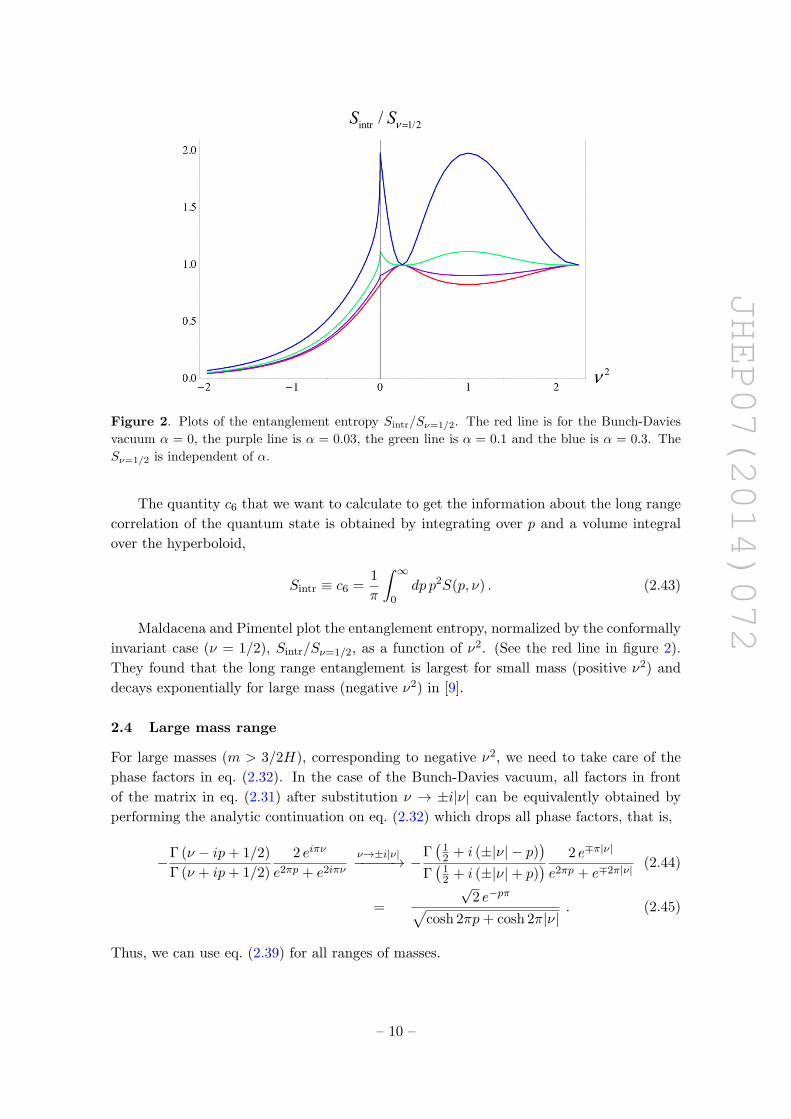
Figure 2. Plots of the entanglement entropy Sintr/Sν=1/2. The red line is for the Bunch-Davies
vacuum α = 0, the purple line is α = 0.03, the green line is α = 0.1 and the blue is α = 0.3. The
Sν=1/2 is independent of α.
The quantity c6 that we want to calculate to get the information about the long range
correlation of the quantum state is obtained by integrating over p and a volume integral
over the hyperboloid,
Sintr ≡ c6 =1
π
∫ ∞0
dp p2S(p, ν) . (2.43)
Maldacena and Pimentel plot the entanglement entropy, normalized by the conformally
invariant case (ν = 1/2), Sintr/Sν=1/2, as a function of ν2. (See the red line in figure 2).
They found that the long range entanglement is largest for small mass (positive ν2) and
decays exponentially for large mass (negative ν2) in [9].
2.4 Large mass range
For large masses (m > 3/2H), corresponding to negative ν2, we need to take care of the
phase factors in eq. (2.32). In the case of the Bunch-Davies vacuum, all factors in front
of the matrix in eq. (2.31) after substitution ν → ±i|ν| can be equivalently obtained by
performing the analytic continuation on eq. (2.32) which drops all phase factors, that is,
−Γ (ν − ip+ 1/2)
Γ (ν + ip+ 1/2)
2 eiπν
e2πp + e2iπν
ν→±i|ν|−−−−−→ −Γ(
12 + i (±|ν| − p)
)Γ(
12 + i (±|ν|+ p)
) 2 e∓π|ν|
e2πp + e∓2π|ν| (2.44)
=
√2 e−pπ√
cosh 2πp+ cosh 2π|ν|. (2.45)
Thus, we can use eq. (2.39) for all ranges of masses.
– 10 –
JHEP07(2014)072
2.5 Super-curvature modes
So far, we have considered only continuous spectrum for the eigenvalue p. However, it
is known that there exists a discrete mode p = i (ν − 1/2) in the spectrum, the so-called
super-curvature mode [21]. We need to worry about it, namely, the super-curvature mode
may contribute to the long-range entanglement of a quantum state. However, since the
super-curvature modes exist with a spacial value of p = i (ν − 1/2), it is plausible that the
integration would not produce a finite measure unless the super-curvature modes behaves
as delta-functions due to unnormalizable nature of the super-curvature mode. It would be
interesting to investigate this more precisely.
3 Entanglement entropy of α-vacua
In the previous section, we reviewed the entanglement entropy in the Bunch-Davies vac-
uum [9]. Here, we extend the calculation to more general α-vacua, which corresponds to
a state filled with particles from the point of view of the Bunch-Davies vacuum [25, 26].
The α-vacua are also de Sitter invariant, so we can use the same mapping in figure 1 that
was used to define a simple representation of the two subspaces. We will examine if the
long range entanglement is affected by the state in which particles are pair-created in the
vacuum.
3.1 α-vacua
The CPT invariant α-vacua can be parametrized by a single positive real parameter α.
The Bunch-Davies vacuum is realized when α = 0. The mode function is obtained by
the Bogoliubov transformation from the mode function of the Bunch-Davies vacuum in
eq. (2.19) such as
Uσp`m(t, r,Ω) = coshαuσp`m(t, r,Ω) + sinhαu∗σp`m(t, r,Ω) . (3.1)
The relation between the annihilation operators in the α-vacua and the Bunch-Davies
vacuum is also defined by the Bogoliubov transformation
dσ = coshαaσ − sinhαa†σ . (3.2)
The definition of an α-vacuum is then simply
dσ|α〉 = 0 . (3.3)
The scalar field in eq. (2.18) is expanded by those mode functions and operators
φ(t, r,Ω) =∑σ,`,m
∫dp[dσp`m Uσp`m(t, r,Ω) + d†σp`m U
∗σp`m(t, r,Ω)
]. (3.4)
– 11 –
JHEP07(2014)072
It is helpful to note that the α-vacua are directly related to the Bunch-Davies vacuum
and the R and L-vacua as
|α〉 = exp
[1
2tanhα a†σa
†σ
]|BD〉
= exp
1
2tanhα
∑q=R,L
[ξ∗qσ b
†q + δqσ bq
] ∑q=R,L
[ξ∗qσ b
†q + δqσ bq
]× exp
1
2
∑i,j=R,L
mij b†i b†j
|R〉|L〉 , (3.5)
where we used eqs. (2.29) and (2.30) and pairs of σ are summed over. It is well known that
the α-vacua are nothing but squeezed states. Looking at the above formula, we see that
the α-vacua should create extra correlations across the R and L sub-systems.
3.2 Bogoliubov transformation to R, L-vacua
We calculate the entanglement entropy of α-vacua with the setup of the previous subsection.
The calculation is completely parallel to that of the Bunch-Davies vacuum but we start
with a different set of creation and annihilation operators.
We first to find a relation between operators of α-vacua and ones of R (or L) vacua.
Plugging eq. (2.29) into eq. (3.2), we get the relation
dσ =∑q=R,L
[coshα ξqσ − sinhα δqσ bq +
coshα δ∗qσ − sinhα ξ∗qσ
b†q
]. (3.6)
Comparing this with eq. (2.29), we find that the Bogoliubov transformation for the original
ξqσ and δ∗qσ is
ξqσ → coshα ξqσ − sinhα δqσ , δ∗qσ → coshα δ∗qσ − sinhα ξ∗qσ . (3.7)
The Bogoliubov transformation between α-vacua and R (or L) vacua can be found by the
consistency of the definition of the α-vacua eq. (3.3) of
|α 〉 = exp
1
2
∑i,j=R,L
mij b†i b†j
|R〉|L〉 , (3.8)
provided
mij = − coshα δ∗iσ − sinhα ξ∗iσ coshα ξ − sinhα δ −1σ j , (3.9)
where we used the first equation in eq. (2.31) and eq. (3.7). Using the expression of ξ and
δ given by eq. (2.28), we get
mij = −Γ(ν − ip+ 1
2
)Γ(ν + ip+ 1
2
) 2
e2πp (coshα− sinhα e−2πp)2 + e2iπν (coshα+ sinhα e−2iπν)2
×
(DRR DRL
DLR DLL
), (3.10)
– 12 –
JHEP07(2014)072
where
DRR = DLL =(cosh2 α eiπν + sinh2 α e−iπν
)cosπν − sinh 2α sinh2 πp , (3.11)
DRL = DLR = i[cosh2 α eiπν + sinh2 α e−iπν + sinh 2α cosπν
]sinhπp . (3.12)
3.3 Diagonalization
In order to trace out the R (or L) degree of freedom, the density matrix has to be diagonal-
ized as in the form eq. (2.40). To do this, we need to perform the Bogoliubov transformation
eq. (2.33) again to get the relation
|α〉 = exp(γp c
†L c†R
)|R′〉|L′〉 . (3.13)
The consistency conditions for eq. (3.13)
cR |α〉 = γp c†L |α〉 , cL |α〉 = γp c
†R |α〉 , (3.14)
gives rise to the system of four homogeneous equations eqs. (2.36) and (2.37). Here, ω and
ζ in the case of α-vacua are read off from eq. (3.10) and
ω ≡ mRR = mLL , ζ ≡ mRL = mLR . (3.15)
We see that ω and ζ are not real and pure imaginary respectively for positive ν2, which
are different from the case of de Sitter vacuum. Thus we cannot reduce the system of four
homogeneous equation eqs. (2.36) and (2.37) into two by setting v∗ = v and u∗ = u in the
case of α-vacua. We need to solve the system of four homegeneous equations for positive
ν2, with conditions |u|2 − |v|2 = 1 and |u|2 − |v|2 = 1.
Fortunately, we find a non-trivial solution of γp of this system:
|γp|2 =1
2|ζ|2
[− ω2ζ∗2 − ω∗2ζ2 + |ω|4 − 2|ω|2 + 1 + |ζ|4
−√
(ω2ζ∗2 + ω∗2ζ2 − |ω|4 + 2|ω|2 − 1− |ζ|4 )2 − 4|ζ|4]. (3.16)
This recovers eq. (2.38) when α = 0, ω∗ = ω and ζ∗ = −ζ. So these results are analytically
consistent. For negative ν2, we find eq. (3.16) is analytic under substitution ν → −i|ν|.2
This can be checked as follows. As we will see in section 3.5, ω becomes real and ζ becomes
pure imaginary for negative ν2. So we can reduce the system of four equations into that
of two equation as in the case of the Bunch-Davies vacuum. We can plot from ν2 < 0
by using eq. (2.38) and we find the plots agree with the ones obtained by using analytic
continuation of eq. (3.16).
2Here, we have two choices of ν → ±i|ν|. In the case of the Bunch-Davies vacuum, the result doesn’t
change whichever sign we choose. In the α-vacua case, however, we find that the substitution i|ν| produces
the divergence where |γp| ≥ 1.
– 13 –
JHEP07(2014)072
intr 1/2/S Sν =
Reν
Imν
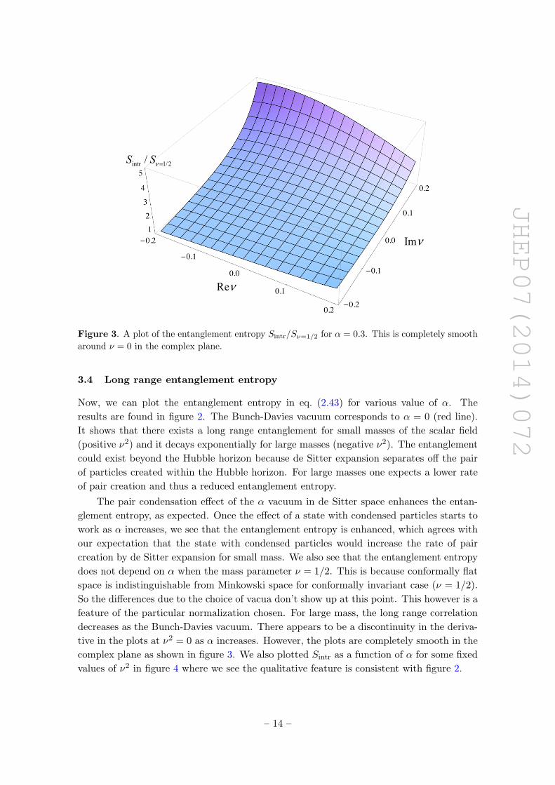
Figure 3. A plot of the entanglement entropy Sintr/Sν=1/2 for α = 0.3. This is completely smooth
around ν = 0 in the complex plane.
3.4 Long range entanglement entropy
Now, we can plot the entanglement entropy in eq. (2.43) for various value of α. The
results are found in figure 2. The Bunch-Davies vacuum corresponds to α = 0 (red line).
It shows that there exists a long range entanglement for small masses of the scalar field
(positive ν2) and it decays exponentially for large masses (negative ν2). The entanglement
could exist beyond the Hubble horizon because de Sitter expansion separates off the pair
of particles created within the Hubble horizon. For large masses one expects a lower rate
of pair creation and thus a reduced entanglement entropy.
The pair condensation effect of the α vacuum in de Sitter space enhances the entan-
glement entropy, as expected. Once the effect of a state with condensed particles starts to
work as α increases, we see that the entanglement entropy is enhanced, which agrees with
our expectation that the state with condensed particles would increase the rate of pair
creation by de Sitter expansion for small mass. We also see that the entanglement entropy
does not depend on α when the mass parameter ν = 1/2. This is because conformally flat
space is indistinguishable from Minkowski space for conformally invariant case (ν = 1/2).
So the differences due to the choice of vacua don’t show up at this point. This however is a
feature of the particular normalization chosen. For large mass, the long range correlation
decreases as the Bunch-Davies vacuum. There appears to be a discontinuity in the deriva-
tive in the plots at ν2 = 0 as α increases. However, the plots are completely smooth in the
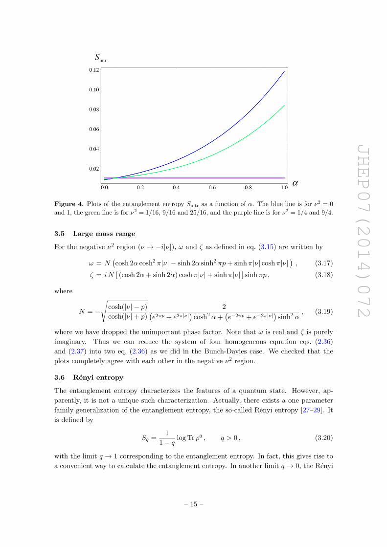
complex plane as shown in figure 3. We also plotted Sintr as a function of α for some fixed
values of ν2 in figure 4 where we see the qualitative feature is consistent with figure 2.
– 14 –
JHEP07(2014)072
intrS
α
Figure 4. Plots of the entanglement entropy Sintr as a function of α. The blue line is for ν2 = 0
and 1, the green line is for ν2 = 1/16, 9/16 and 25/16, and the purple line is for ν2 = 1/4 and 9/4.
3.5 Large mass range
For the negative ν2 region (ν → −i|ν|), ω and ζ as defined in eq. (3.15) are written by
ω = N(cosh 2α cosh2 π|ν| − sinh 2α sinh2 πp+ sinhπ|ν| coshπ|ν|
), (3.17)
ζ = iN [ (cosh 2α+ sinh 2α) coshπ|ν|+ sinhπ|ν| ] sinhπp , (3.18)
where
N = −
√cosh(|ν| − p)cosh(|ν|+ p)
2(e2πp + e2π|ν|
)cosh2 α+
(e−2πp + e−2π|ν|
)sinh2 α
, (3.19)
where we have dropped the unimportant phase factor. Note that ω is real and ζ is purely
imaginary. Thus we can reduce the system of four homogeneous equation eqs. (2.36)
and (2.37) into two eq. (2.36) as we did in the Bunch-Davies case. We checked that the
plots completely agree with each other in the negative ν2 region.
3.6 Renyi entropy
The entanglement entropy characterizes the features of a quantum state. However, ap-
parently, it is not a unique such characterization. Actually, there exists a one parameter
family generalization of the entanglement entropy, the so-called Renyi entropy [27–29]. It
is defined by
Sq =1
1− qlog Tr ρq , q > 0 , (3.20)
with the limit q → 1 corresponding to the entanglement entropy. In fact, this gives rise to
a convenient way to calculate the entanglement entropy. In another limit q → 0, the Renyi
– 15 –
JHEP07(2014)072
2ν
,intr , 1/2/q qS S ν =
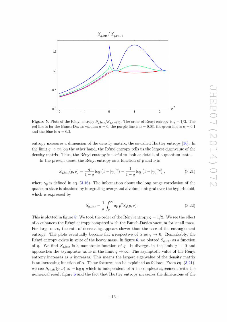
Figure 5. Plots of the Renyi entropy Sq,intr/Sq,ν=1/2. The order of Renyi entropy is q = 1/2. The
red line is for the Bunch-Davies vacuum α = 0, the purple line is α = 0.03, the green line is α = 0.1
and the blue is α = 0.3.
entropy measures a dimension of the density matrix, the so-called Hartley entropy [30]. In
the limit q →∞, on the other hand, the Renyi entropy tells us the largest eigenvalue of the
density matrix. Thus, the Renyi entropy is useful to look at details of a quantum state.
In the present cases, the Renyi entropy as a function of p and ν is
Sq,intr(p, ν) =q
1− qlog(1− |γp|2
)− 1
1− qlog(1− |γp|2q
), (3.21)
where γp is defined in eq. (3.16). The information about the long range correlation of the
quantum state is obtained by integrating over p and a volume integral over the hyperboloid,
which is expressed by
Sq,intr =1
π
∫ ∞0
dp p2Sq(p, ν) . (3.22)
This is plotted in figure 5. We took the order of the Renyi entropy q = 1/2. We see the effect
of α enhances the Renyi entropy compared with the Bunch-Davies vacuum for small mass.
For large mass, the rate of decreasing appears slower than the case of the entanglement
entropy. The plots eventually become flat irrespective of α as q → 0. Remarkably, the
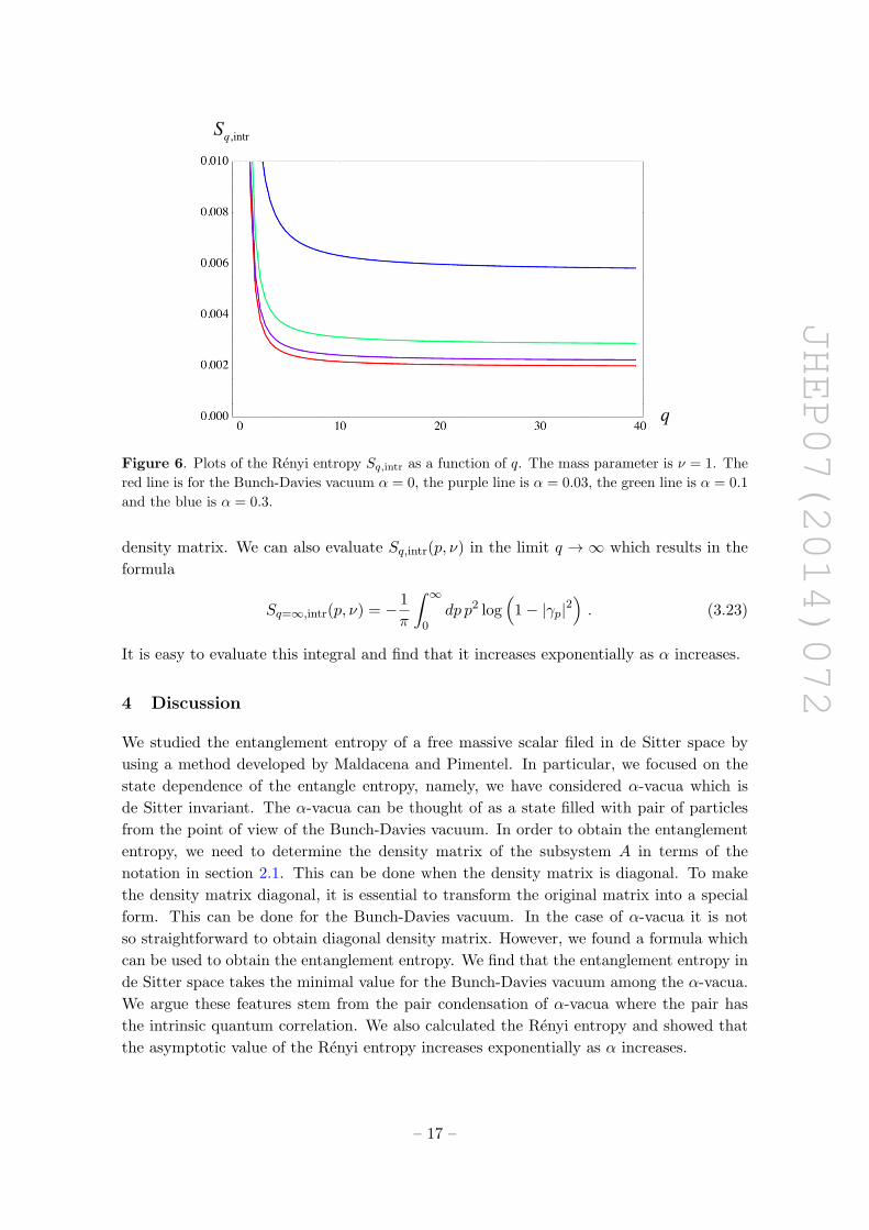
Renyi entropy exists in spite of the heavy mass. In figure 6, we plotted Sq,intr as a function
of q. We find Sq,intr is a monotonic function of q. It diverges in the limit q → 0 and
approaches the asymptotic value in the limit q → ∞. The asymptotic value of the Renyi
entropy increases as α increases. This means the largest eigenvalue of the density matrix
is an increasing function of α. These features can be explained as follows. From eq. (3.21),
we see Sq,intr(p, ν) ∝ − log q which is independent of α in complete agreement with the
numerical result figure 6 and the fact that Hartley entropy measures the dimensions of the
– 16 –
JHEP07(2014)072
q
,intrqS
Figure 6. Plots of the Renyi entropy Sq,intr as a function of q. The mass parameter is ν = 1. The
red line is for the Bunch-Davies vacuum α = 0, the purple line is α = 0.03, the green line is α = 0.1
and the blue is α = 0.3.
density matrix. We can also evaluate Sq,intr(p, ν) in the limit q → ∞ which results in the
formula
Sq=∞,intr(p, ν) = − 1
π
∫ ∞0
dp p2 log(
1− |γp|2). (3.23)
It is easy to evaluate this integral and find that it increases exponentially as α increases.
4 Discussion
We studied the entanglement entropy of a free massive scalar filed in de Sitter space by
using a method developed by Maldacena and Pimentel. In particular, we focused on the
state dependence of the entangle entropy, namely, we have considered α-vacua which is
de Sitter invariant. The α-vacua can be thought of as a state filled with pair of particles
from the point of view of the Bunch-Davies vacuum. In order to obtain the entanglement
entropy, we need to determine the density matrix of the subsystem A in terms of the
notation in section 2.1. This can be done when the density matrix is diagonal. To make
the density matrix diagonal, it is essential to transform the original matrix into a special
form. This can be done for the Bunch-Davies vacuum. In the case of α-vacua it is not
so straightforward to obtain diagonal density matrix. However, we found a formula which
can be used to obtain the entanglement entropy. We find that the entanglement entropy in
de Sitter space takes the minimal value for the Bunch-Davies vacuum among the α-vacua.
We argue these features stem from the pair condensation of α-vacua where the pair has
the intrinsic quantum correlation. We also calculated the Renyi entropy and showed that
the asymptotic value of the Renyi entropy increases exponentially as α increases.
– 17 –
JHEP07(2014)072
In terms of future extensions of this work, one of the most pressing would be a holo-
graphic interpretation along the lines of the work of Maldacena and Pimentel for the
Bunch-Davies vacuum in [9]. To summarize their argument; a free field theory on a curved
de Sitter space
ds2 = dw2 + sinh2w[−dt2 + cosh2 t
(dθ2 + cos2 θ dΩ2
)], (4.1)
can be investigated in a holographic context by treating the de Sitter space as the boundary
of an anti-de Sitter (AdS) bulk which can then be considered as the gravitational dual [31,
32]. Here, dΩ2 is the metric of a two-sphere and w, t, θ are a radial, a time, and an angular
coordinate, respectively. Then, following Ryu and Takayanagi [7], they match the field
theory computation of the entanglement entropy to the area of an appropriate minimal
surface in the AdS space. The minimal surface is identified as the surface t = constant and
θ = 0. Starting with a conformally coupled scalar (ν = 1/2), they generalize the model to
non-conformal theories in this holographic scheme. Then, the bulk geometry is modified as
ds2 = dw2 + a2(w) ds2dS4 , (4.2)
where ds2dS4 is a four-dimensional de Sitter metric and the function a(w) is determined by
solving the Einstein equation with the scalar field. The surface we should take is the one
at θ = 0, t = t(w) which extremizes the area
A = VS2
∫a2 cosh2 t(w)
√dw2 − a2dt2 , (4.3)
where VS2 is two-volume. It would be of great interest to understand how this line of
reasoning is modified for α-vacua.
The first hurdle to such a holographic computation of the entanglement entropy of
the α-vacua in a strongly coupled phase is the lack of clarity as to what precisely the
gravity duals of a field theory on such α backgrounds are beyond the fact that they will
likely be some one-parameter deformation of AdS. Nevertheless, having demonstrated that
at ν = 1/2 the entanglement entropy is α-independent, we believe that in this case, the
Maldacena-Pimentel argument should go through essentially unchanged since the latter
does not require a choice of vacuum. More generally though, as we saw above, the entan-
glement entropy of α-vacua is decidedly different from that of the Bunch-Davies vacuum.
Hence, we expect the three-dimensional area at θ = 0, t = t(w) in the AdS bulk must
be further deformed to match the entanglement entropy. However, it is not clear how to
implement this state dependence in to the holographic scheme.3 In the conventional case,
the boundary geometry is Minkowski space where we do not have vacuum ambiguity. Now
that there is a continuum of vacua in de Sitter space, we are not sure what surface corre-
sponds to each vacuum. A naive answer is that because there is a difficulty in defining an
interacting field theory on an α-vacuum [15–17] the holographic principle may not lead to
a well-defined gravitational theory. We leave these considerations for future investigation.
3There is a possible approach to this direction in [33].
– 18 –
JHEP07(2014)072
Acknowledgments
We would very much like to thank Juan Maldacena and Guilherme Pimentel for their
invaluable advice and assistance during the writing of this paper. This work was supported
in part by funding from the University Research Council of the University of Cape Town,
Grants-in-Aid for Scientific Research (C) No.25400251 and Grants-in-Aid for Scientific
Research on Innovative Areas No.26104708. JM is supported by the National Research
Foundation of South Africa through the IPRR and CPRR programs.
Open Access. This article is distributed under the terms of the Creative Commons
Attribution License (CC-BY 4.0), which permits any use, distribution and reproduction in
any medium, provided the original author(s) and source are credited.
References
[1] R. Horodecki, P. Horodecki, M. Horodecki and K. Horodecki, Quantum entanglement, Rev.
Mod. Phys. 81 (2009) 865 [quant-ph/0702225] [INSPIRE].
[2] A. Einstein, B. Podolsky and N. Rosen, Can quantum mechanical description of physical
reality be considered complete?, Phys. Rev. 47 (1935) 777 [INSPIRE].
[3] S.R. Coleman and F. De Luccia, Gravitational Effects on and of Vacuum Decay, Phys. Rev.
D 21 (1980) 3305 [INSPIRE].
[4] J. Garriga, S. Kanno, M. Sasaki, J. Soda and A. Vilenkin, Observer dependence of bubble
nucleation and Schwinger pair production, JCAP 12 (2012) 006 [arXiv:1208.1335]
[INSPIRE].
[5] J. Garriga, S. Kanno and T. Tanaka, Rest frame of bubble nucleation, JCAP 06 (2013) 034
[arXiv:1304.6681] [INSPIRE].
[6] M.B. Frob et al., Schwinger effect in de Sitter space, JCAP 04 (2014) 009
[arXiv:1401.4137] [INSPIRE].
[7] S. Ryu and T. Takayanagi, Holographic derivation of entanglement entropy from AdS/CFT,
Phys. Rev. Lett. 96 (2006) 181602 [hep-th/0603001] [INSPIRE].
[8] T. Takayanagi, Entanglement Entropy from a Holographic Viewpoint, Class. Quant. Grav. 29
(2012) 153001 [arXiv:1204.2450] [INSPIRE].
[9] J. Maldacena and G.L. Pimentel, Entanglement entropy in de Sitter space, JHEP 02 (2013)
038 [arXiv:1210.7244] [INSPIRE].
[10] A. Ashoorioon, K. Dimopoulos, M.M. Sheikh-Jabbari and G. Shiu, Non-Bunch-Davis Initial
State Reconciles Chaotic Models with BICEP and Planck, arXiv:1403.6099 [INSPIRE].
[11] BICEP2 collaboration, P.A.R. Ade et al., Detection of B-Mode Polarization at Degree
Angular Scales by BICEP2, Phys. Rev. Lett. 112 (2014) 241101 [arXiv:1403.3985]
[INSPIRE].
[12] G.W. Gibbons and S.W. Hawking, Cosmological Event Horizons, Thermodynamics and
Particle Creation, Phys. Rev. D 15 (1977) 2738 [INSPIRE].
[13] M. Spradlin, A. Strominger and A. Volovich, Les Houches lectures on de Sitter space,
hep-th/0110007 [INSPIRE].
– 19 –
JHEP07(2014)072
[14] R. Bousso, A. Maloney and A. Strominger, Conformal vacua and entropy in de Sitter space,
Phys. Rev. D 65 (2002) 104039 [hep-th/0112218] [INSPIRE].
[15] U.H. Danielsson, On the consistency of de Sitter vacua, JHEP 12 (2002) 025
[hep-th/0210058] [INSPIRE].
[16] M.B. Einhorn and F. Larsen, Squeezed states in the de Sitter vacuum, Phys. Rev. D 68
(2003) 064002 [hep-th/0305056] [INSPIRE].
[17] H. Collins, R. Holman and M.R. Martin, The Fate of the α-vacuum, Phys. Rev. D 68 (2003)
124012 [hep-th/0306028] [INSPIRE].
[18] C. Holzhey, F. Larsen and F. Wilczek, Geometric and renormalized entropy in conformal
field theory, Nucl. Phys. B 424 (1994) 443 [hep-th/9403108] [INSPIRE].
[19] L. Bombelli, R.K. Koul, J. Lee and R.D. Sorkin, A Quantum Source of Entropy for Black
Holes, Phys. Rev. D 34 (1986) 373 [INSPIRE].
[20] M. Srednicki, Entropy and area, Phys. Rev. Lett. 71 (1993) 666 [hep-th/9303048] [INSPIRE].
[21] M. Sasaki, T. Tanaka and K. Yamamoto, Euclidean vacuum mode functions for a scalar field
on open de Sitter space, Phys. Rev. D 51 (1995) 2979 [gr-qc/9412025] [INSPIRE].
[22] T.S. Bunch and P.C.W. Davies, Quantum Field Theory in de Sitter Space: Renormalization
by Point Splitting, Proc. Roy. Soc. Lond. A 360 (1978) 117 [INSPIRE].
[23] N.A. Chernikov and E.A. Tagirov, Quantum theory of scalar fields in de Sitter space-time,
Ann. I. H. Poincare A 9 (1968) 109.
[24] J.B. Hartle and S.W. Hawking, Wave Function of the Universe, Phys. Rev. D 28 (1983)
2960 [INSPIRE].
[25] E. Mottola, Particle Creation in de Sitter Space, Phys. Rev. D 31 (1985) 754 [INSPIRE].
[26] B. Allen, Vacuum States in de Sitter Space, Phys. Rev. D 32 (1985) 3136 [INSPIRE].
[27] A. Renyi, On measures of information and entropy, in Proceedings of the 4th Berkeley
Symposium on Mathematics, Statistics and Probability, vol. 1, University of California Press,
Berkeley CA U.S.A. (1961), pg. 547.
[28] A. Renyi, On the foundations of information theory, Rev. Int. Stat. Inst. 33 (1965) 1.
[29] I.R. Klebanov, S.S. Pufu, S. Sachdev and B.R. Safdi, Renyi Entropies for Free Field
Theories, JHEP 04 (2012) 074 [arXiv:1111.6290] [INSPIRE].
[30] M. Headrick, Entanglement Renyi entropies in holographic theories, Phys. Rev. D 82 (2010)
126010 [arXiv:1006.0047] [INSPIRE].
[31] S. Hawking, J.M. Maldacena and A. Strominger, de Sitter entropy, quantum entanglement
and AdS/CFT, JHEP 05 (2001) 001 [hep-th/0002145] [INSPIRE].
[32] K. Koyama and J. Soda, Strongly coupled CFT in FRW universe from AdS/CFT
correspondence, JHEP 05 (2001) 027 [hep-th/0101164] [INSPIRE].
[33] W. Fischler, S. Kundu and J.F. Pedraza, Entanglement and out-of-equilibrium dynamics in
holographic models of de Sitter QFTs, arXiv:1311.5519 [INSPIRE].
– 20 –