Propagation of errors - Instituto Tecnológico de Aeronáutica · Physics 2BL 7 Histograms and...
36
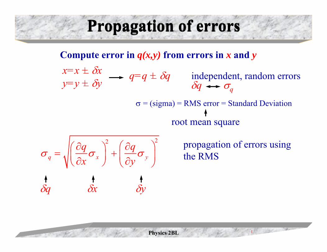
Physics 2BL Physics 2BL 1 Propagation of errors Propagation of errors Compute error in q(x,y) from errors in x and y 2 2 q x y q q x y σ σ σ ⎛ ⎞ ∂ ∂ ⎛ ⎞ = + ⎜ ⎟ ⎜ ⎟ ∂ ∂ ⎝ ⎠ ⎝ ⎠ propagation of errors using the RMS σ = (sigma) = RMS error = Standard Deviation δq δx δy root mean square q=q + δq _ y=y + δy x=x + δx _ _ independent, random errors δq σ q
Transcript of Propagation of errors - Instituto Tecnológico de Aeronáutica · Physics 2BL 7 Histograms and...
Physics 2BLPhysics 2BL 1
Propagation of errorsPropagation of errors
Compute error in q(x,y) from errors in x and y
22
q x yq qx y
σ σ σ⎛ ⎞∂ ∂⎛ ⎞= +⎜ ⎟ ⎜ ⎟∂ ∂⎝ ⎠ ⎝ ⎠
propagation of errors using the RMS
σ = (sigma) = RMS error = Standard Deviation
δq δx δy
root mean square
q=q + δq_
y=y + δyx=x + δx
__ independent, random errors
δq σq
Physics 2BLPhysics 2BL 2
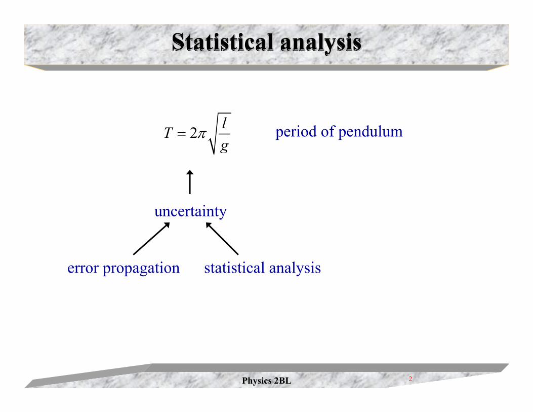
Statistical analysisStatistical analysisStatistical analysis
uncertainty
period of pendulum2 lTg
π=
error propagation statistical analysis
Physics 2BLPhysics 2BL 3
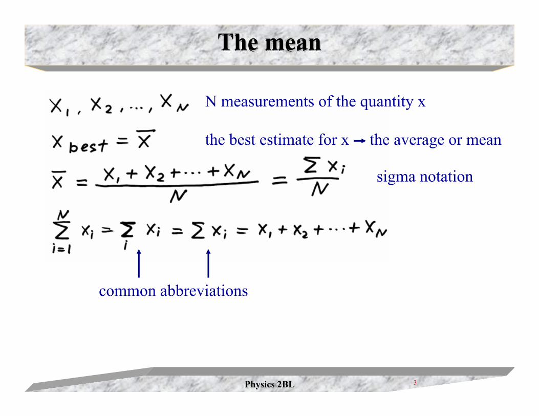
The meanThe meanThe mean
the best estimate for x the average or mean
sigma notation
N measurements of the quantity x
common abbreviations
Physics 2BLPhysics 2BL 4
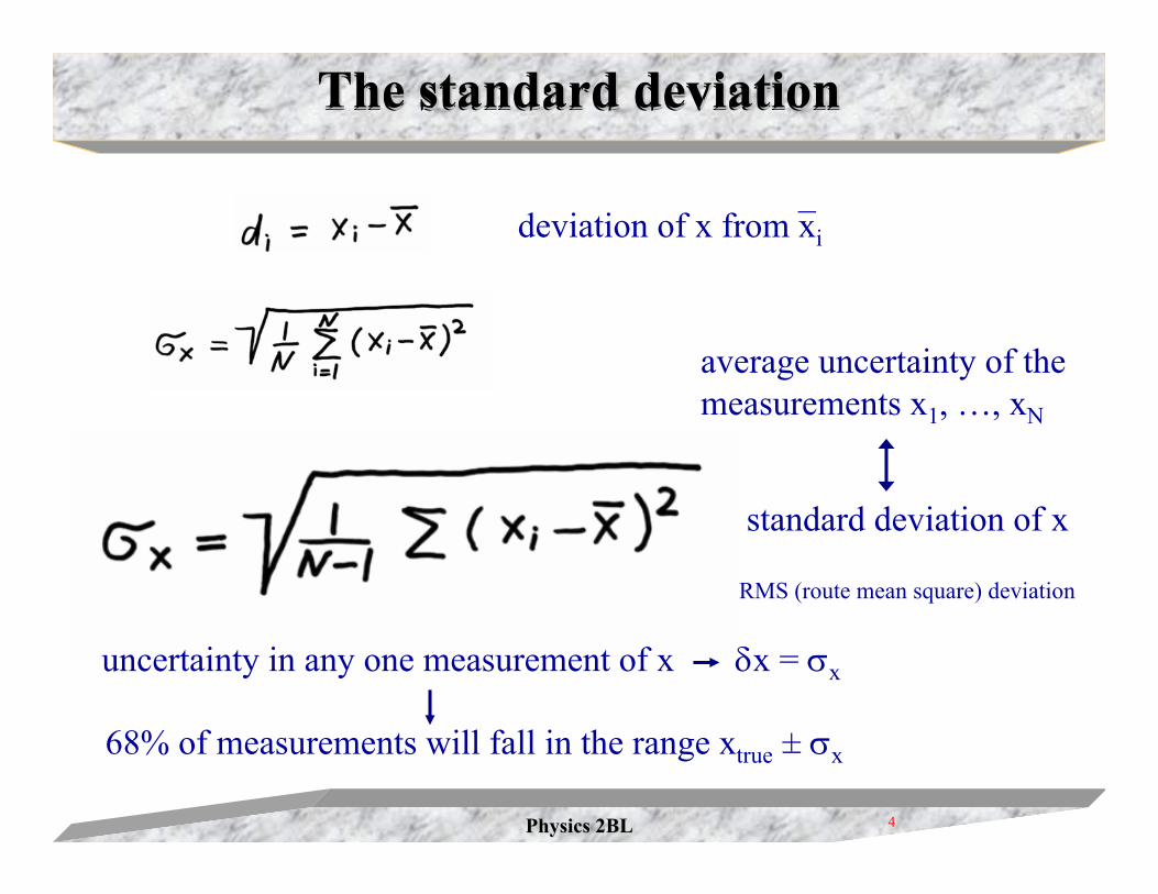
The standard deviationThe standard deviationThe standard deviation
deviation of x from xi
_
standard deviation of x
RMS (route mean square) deviation
average uncertainty of the measurements x1, …, xN
uncertainty in any one measurement of x δx = σx
68% of measurements will fall in the range xtrue + σx_
Physics 2BLPhysics 2BL 5
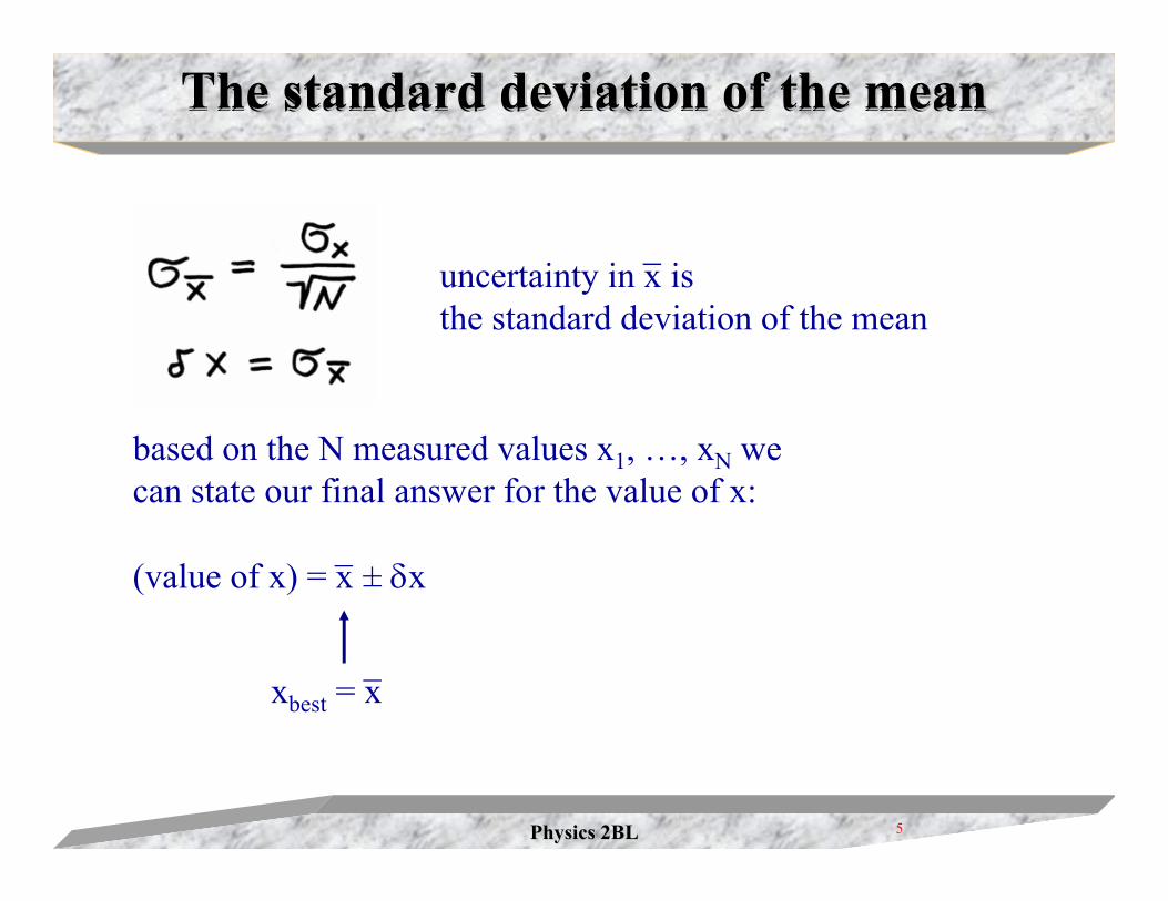
The standard deviation of the meanThe standard deviation of the meanThe standard deviation of the mean
uncertainty in x isthe standard deviation of the mean
_
based on the N measured values x1, …, xN we can state our final answer for the value of x:
(value of x) = x + δx__
xbest = x_
Physics 2BLPhysics 2BL 6
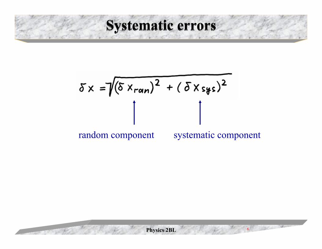
Systematic errorsSystematic errorsSystematic errors
random component systematic component
Physics 2BLPhysics 2BL 7
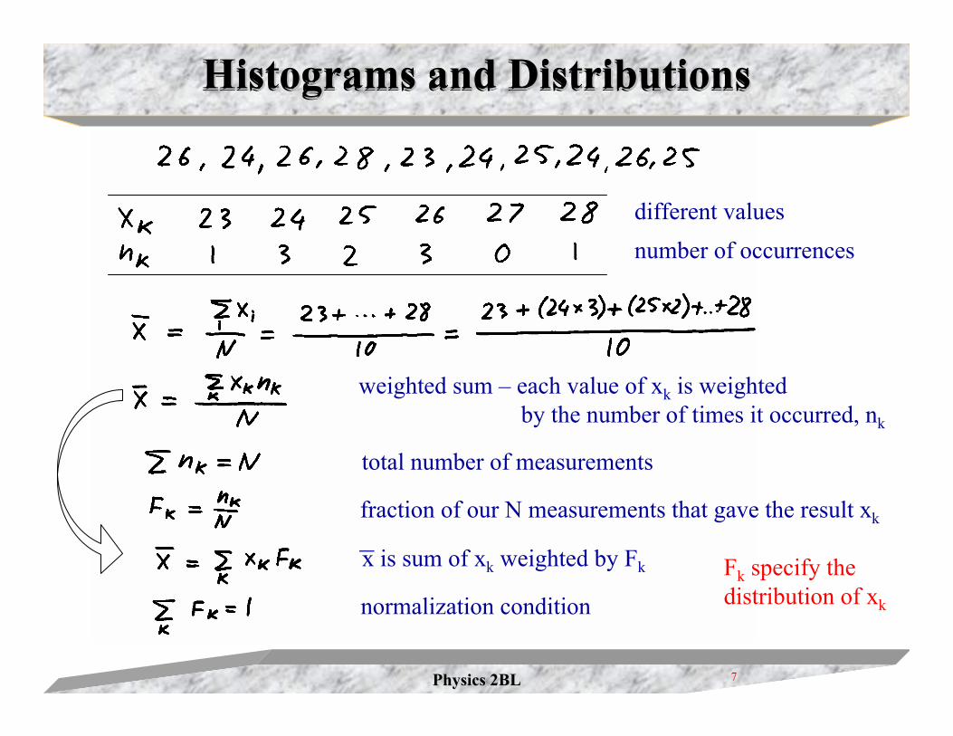
Histograms and DistributionsHistograms and DistributionsHistograms and Distributions
different valuesnumber of occurrences
weighted sum – each value of xk is weighted by the number of times it occurred, nk
total number of measurements
fraction of our N measurements that gave the result xk
normalization condition
x is sum of xk weighted by Fk
_Fk specify the distribution of xk
Physics 2BLPhysics 2BL 8
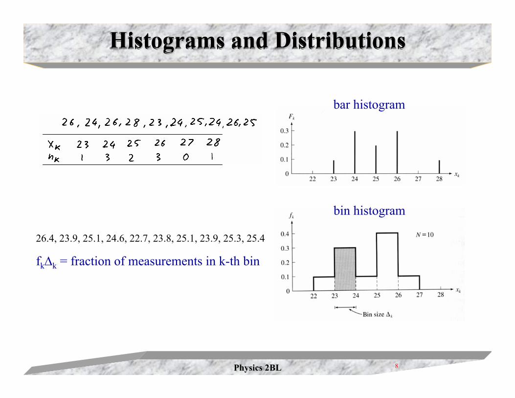
Histograms and DistributionsHistograms and DistributionsHistograms and Distributions
bar histogram
bin histogram
26.4, 23.9, 25.1, 24.6, 22.7, 23.8, 25.1, 23.9, 25.3, 25.4
fk∆k = fraction of measurements in k-th bin
Physics 2BLPhysics 2BL 9
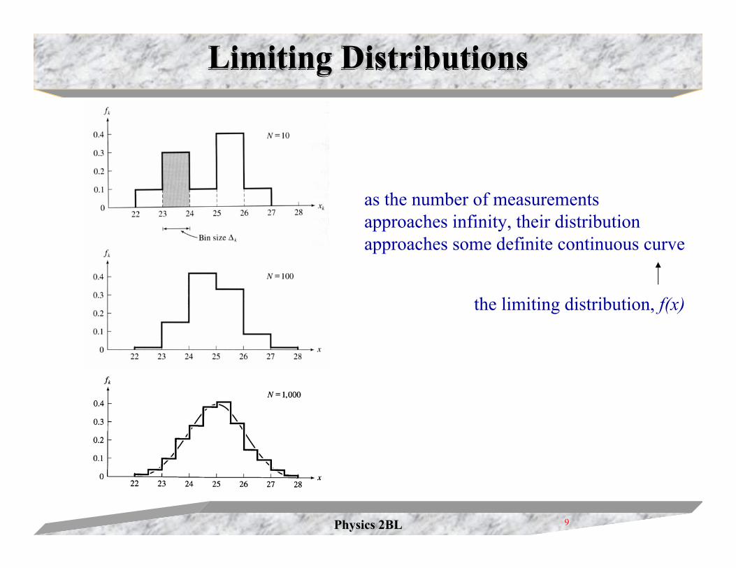
Limiting DistributionsLimiting DistributionsLimiting Distributions
as the number of measurements approaches infinity, their distribution approaches some definite continuous curve
the limiting distribution, f(x)
Physics 2BLPhysics 2BL 10
Limiting DistributionsLimiting DistributionsLimiting Distributions
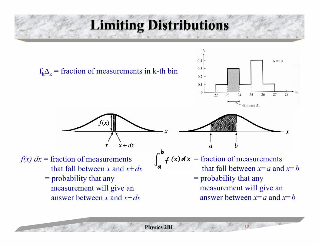
f(x) dx = fraction of measurements that fall between x and x+dx
= probability that any measurement will give an answer between x and x+dx
= fraction of measurements that fall between x=a and x=b
= probability that any measurement will give an answer between x=a and x=b
fk∆k = fraction of measurements in k-th bin
Physics 2BLPhysics 2BL 11
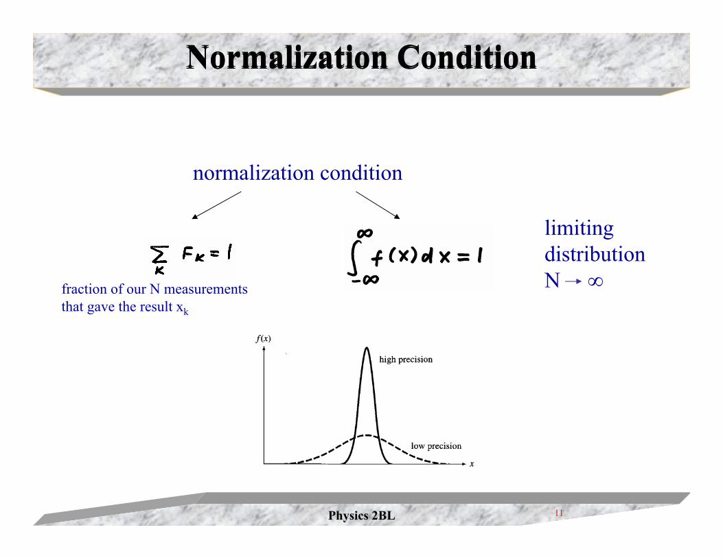
Normalization ConditionNormalization Condition
normalization condition
limiting distribution N ∞fraction of our N measurements
that gave the result xk
Physics 2BLPhysics 2BL 12
The Mean and Standard DeviationThe Mean and Standard DeviationThe Mean and Standard Deviation
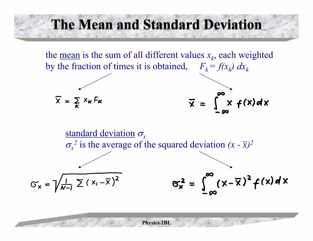
the mean is the sum of all different values xk, each weighted by the fraction of times it is obtained, Fk = f(xk) dxk
standard deviation σxσx
2 is the average of the squared deviation (x - x)2_
Physics 2BLPhysics 2BL 13
The Normal DistributionThe Normal DistributionThe Normal Distribution
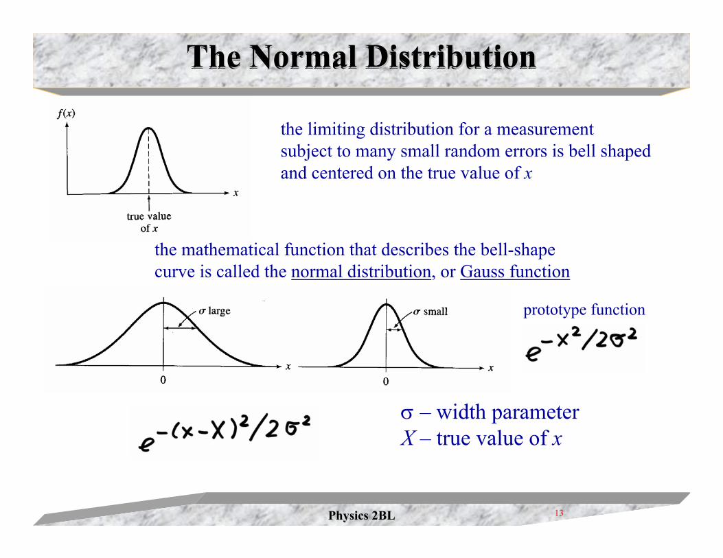
the limiting distribution for a measurement subject to many small random errors is bell shapedand centered on the true value of x
the mathematical function that describes the bell-shape curve is called the normal distribution, or Gauss function
prototype function
σ – width parameterX – true value of x
Physics 2BLPhysics 2BL 14
The Gauss, or Normal DistributionThe Gauss, or Normal DistributionThe Gauss, or Normal Distribution
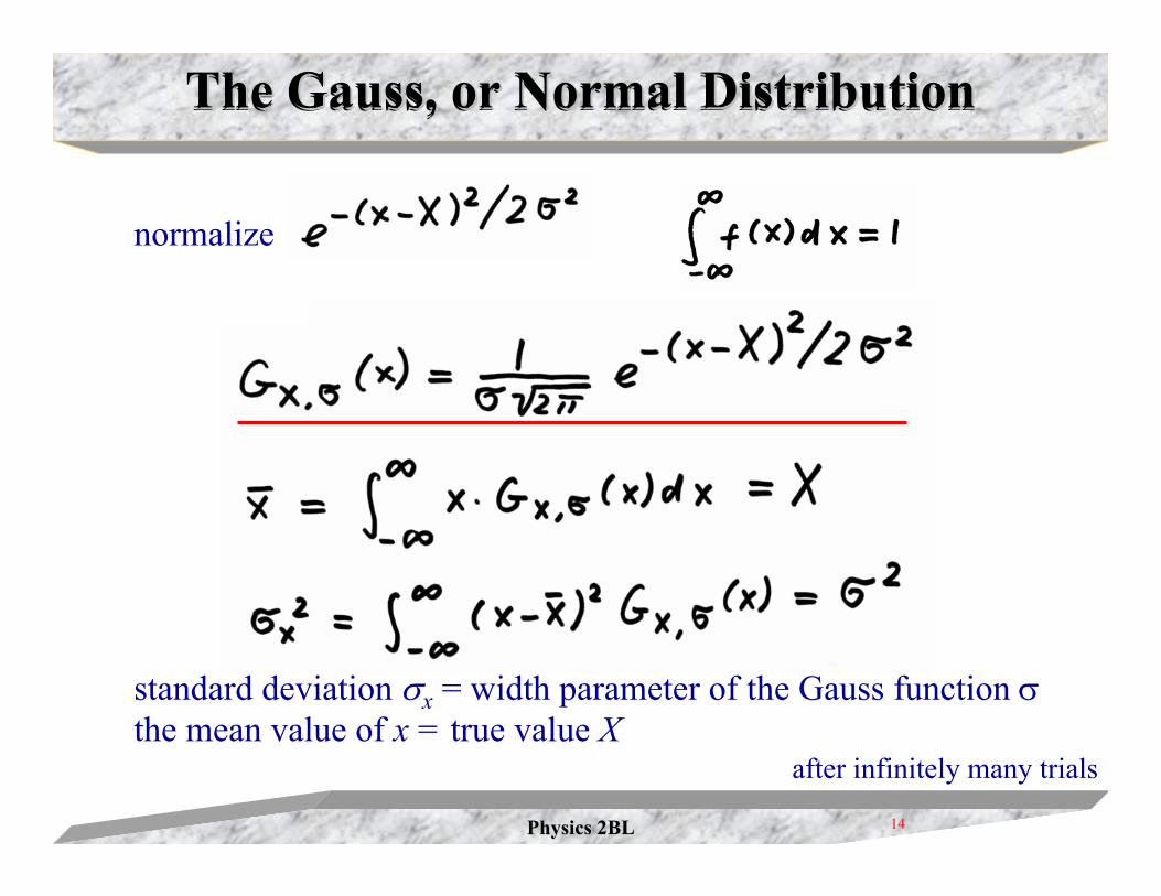
normalize
standard deviation σx = width parameter of the Gauss function σthe mean value of x = true value X
after infinitely many trials
Physics 2BLPhysics 2BL 15
The standard Deviation as 68%Confidence LimitThe standard Deviation as 68%Confidence LimitThe standard Deviation as 68%Confidence Limit
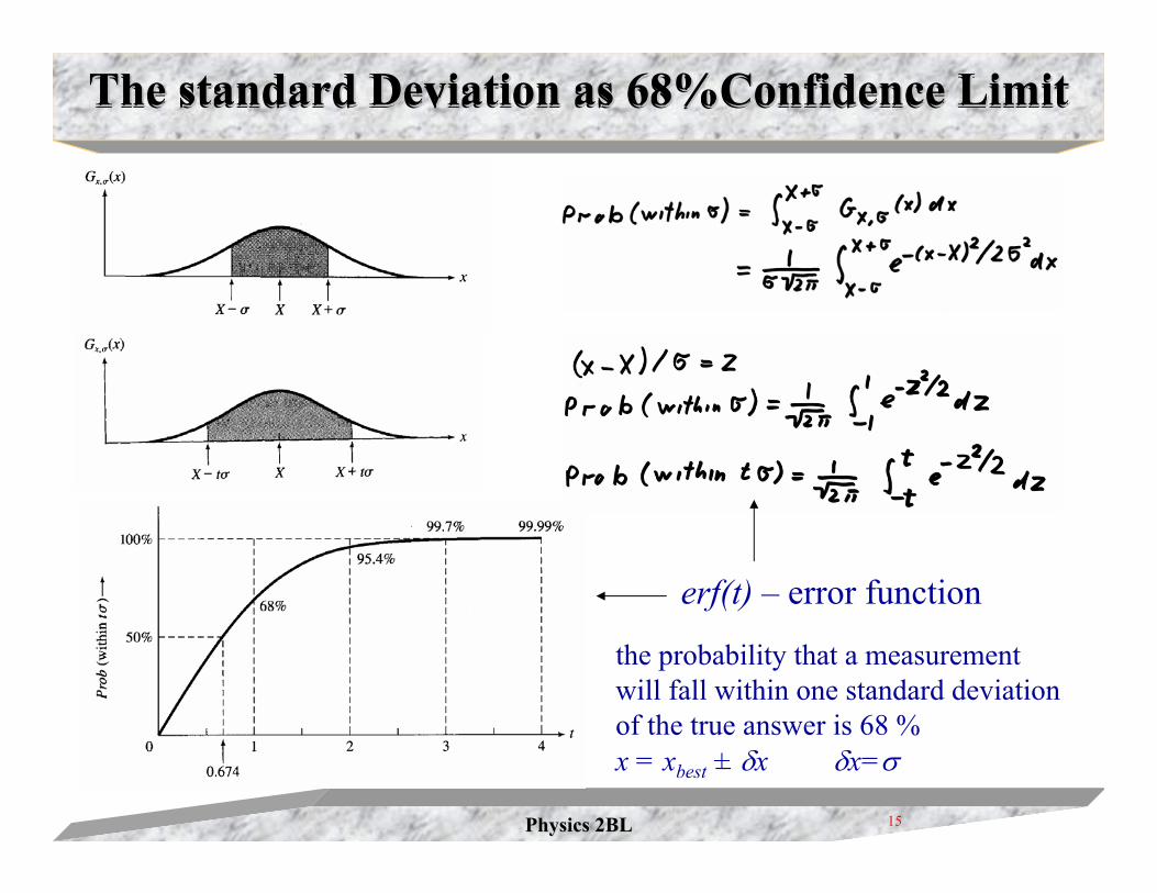
erf(t) – error function
the probability that a measurement will fall within one standard deviationof the true answer is 68 %x = xbest + δx δx=σ_
Physics 2BLPhysics 2BL 16
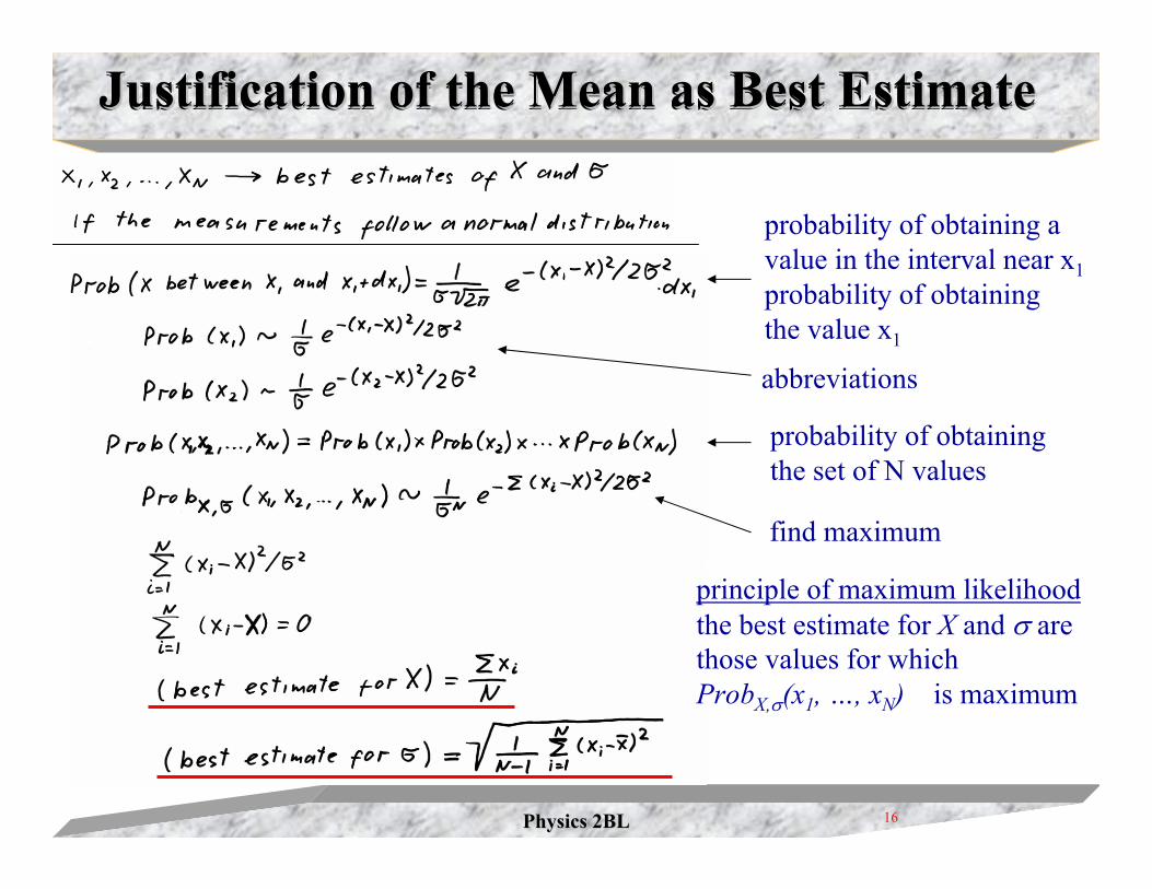
Justification of the Mean as Best EstimateJustification of the Mean as Best EstimateJustification of the Mean as Best Estimate
probability of obtaining avalue in the interval near x1probability of obtaining the value x1
abbreviations
probability of obtaining the set of N values
principle of maximum likelihoodthe best estimate for X and σ are those values for which ProbX,σ(x1, …, xN) is maximum
find maximum
Physics 2BLPhysics 2BL 17
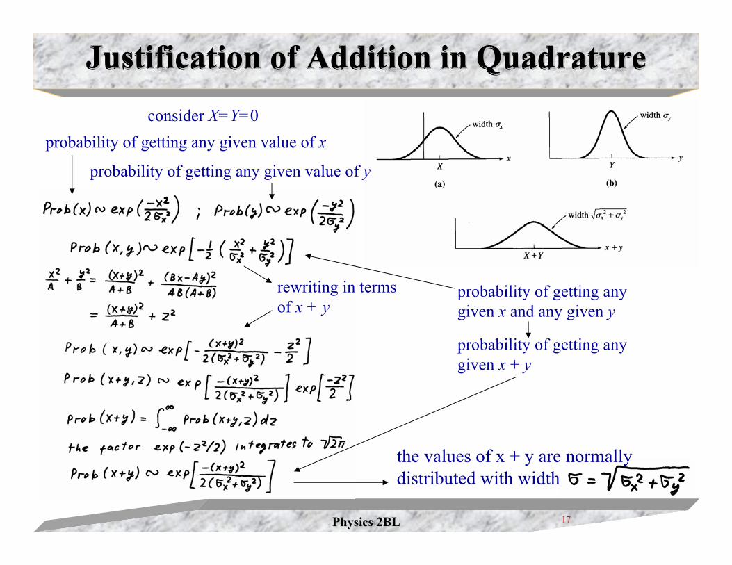
Justification of Addition in QuadratureJustification of Addition in Justification of Addition in QuadratureQuadratureconsider X=Y=0
probability of getting any given value of x
probability of getting any given value of y
probability of getting any given x and any given y
probability of getting any given x + y
rewriting in terms of x + y
the values of x + y are normally distributed with width
Physics 2BLPhysics 2BL 18
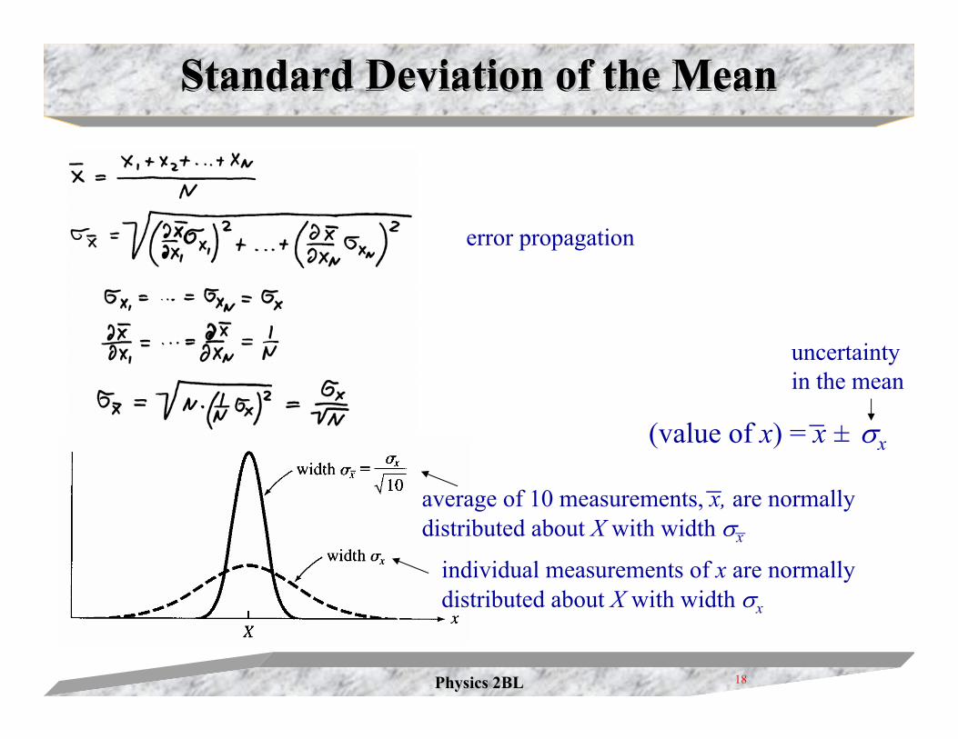
Standard Deviation of the MeanStandard Deviation of the MeanStandard Deviation of the Mean
error propagation
(value of x) = x + σx__
uncertainty in the mean
individual measurements of x are normallydistributed about X with width σx
average of 10 measurements, x, are normallydistributed about X with width σx
__
Physics 2BLPhysics 2BL 19
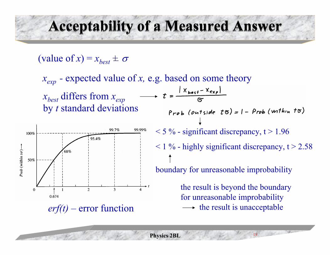
Acceptability of a Measured AnswerAcceptability of a Measured AnswerAcceptability of a Measured Answer
(value of x) = xbest + σ_
xexp - expected value of x, e.g. based on some theory
xbest differs from xexpby t standard deviations
< 5 % - significant discrepancy, t > 1.96
< 1 % - highly significant discrepancy, t > 2.58
boundary for unreasonable improbability
erf(t) – error function
the result is beyond the boundary for unreasonable improbability
the result is unacceptable
Physics 2BLPhysics 2BL 20
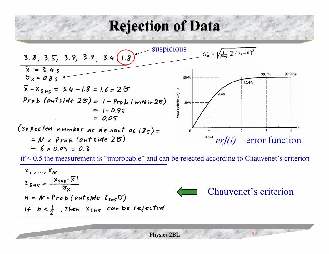
Rejection of DataRejection of DataRejection of Data
erf(t) – error function
Chauvenet’s criterion
if < 0.5 the measurement is “improbable” and can be rejected according to Chauvenet’s criterion
suspicious
Physics 2BLPhysics 2BL 21
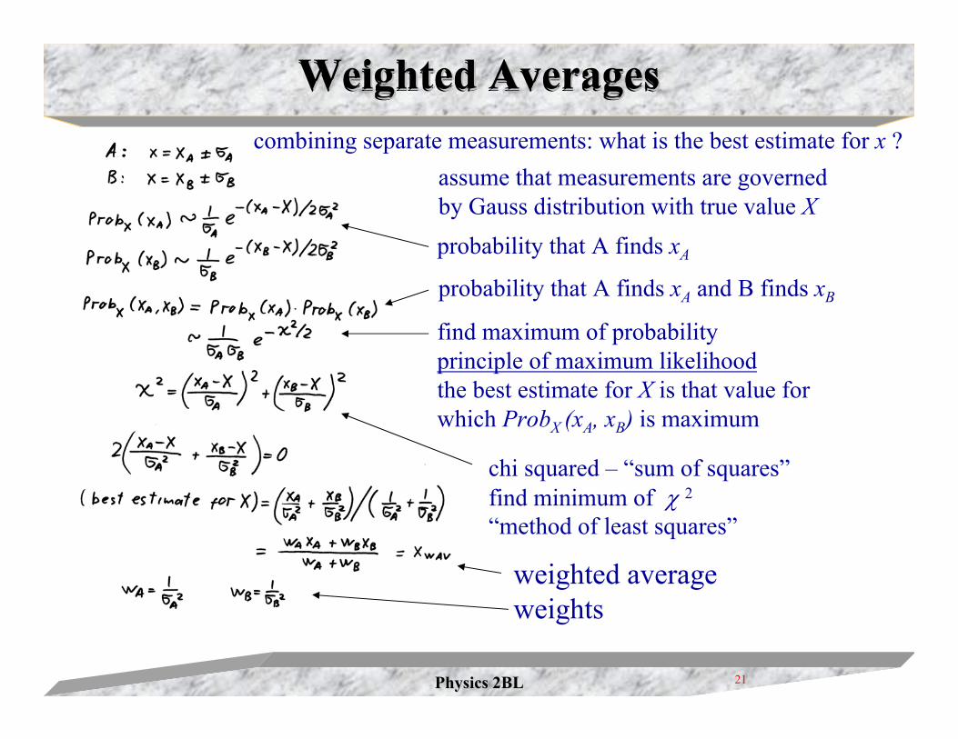
Weighted AveragesWeighted AveragesWeighted Averagescombining separate measurements: what is the best estimate for x ?
probability that A finds xA
find maximum of probabilityprinciple of maximum likelihoodthe best estimate for X is that value for which ProbX (xA, xB) is maximum
assume that measurements are governed by Gauss distribution with true value X
probability that A finds xA and B finds xB
chi squared – “sum of squares”find minimum of χ 2“method of least squares”
weighted averageweights
Physics 2BLPhysics 2BL 22
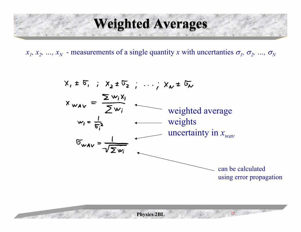
Weighted AveragesWeighted AveragesWeighted Averages
x1, x2, …, xN - measurements of a single quantity x with uncertanties σ1, σ2, …, σN
weighted averageweightsuncertainty in xwav
can be calculated using error propagation
Physics 2BLPhysics 2BL 23
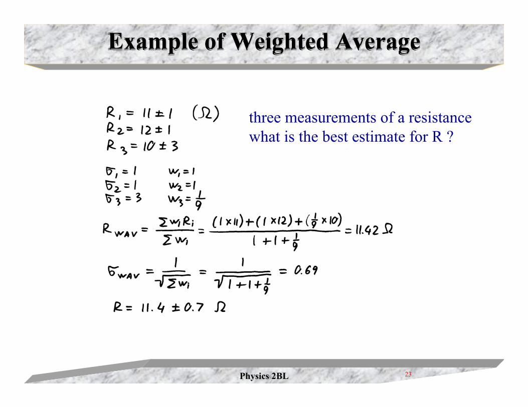
Example of Weighted AverageExample of Weighted AverageExample of Weighted Average
three measurements of a resistancewhat is the best estimate for R ?
Physics 2BLPhysics 2BL 24
Least-Squares FittingLeastLeast--Squares FittingSquares Fitting
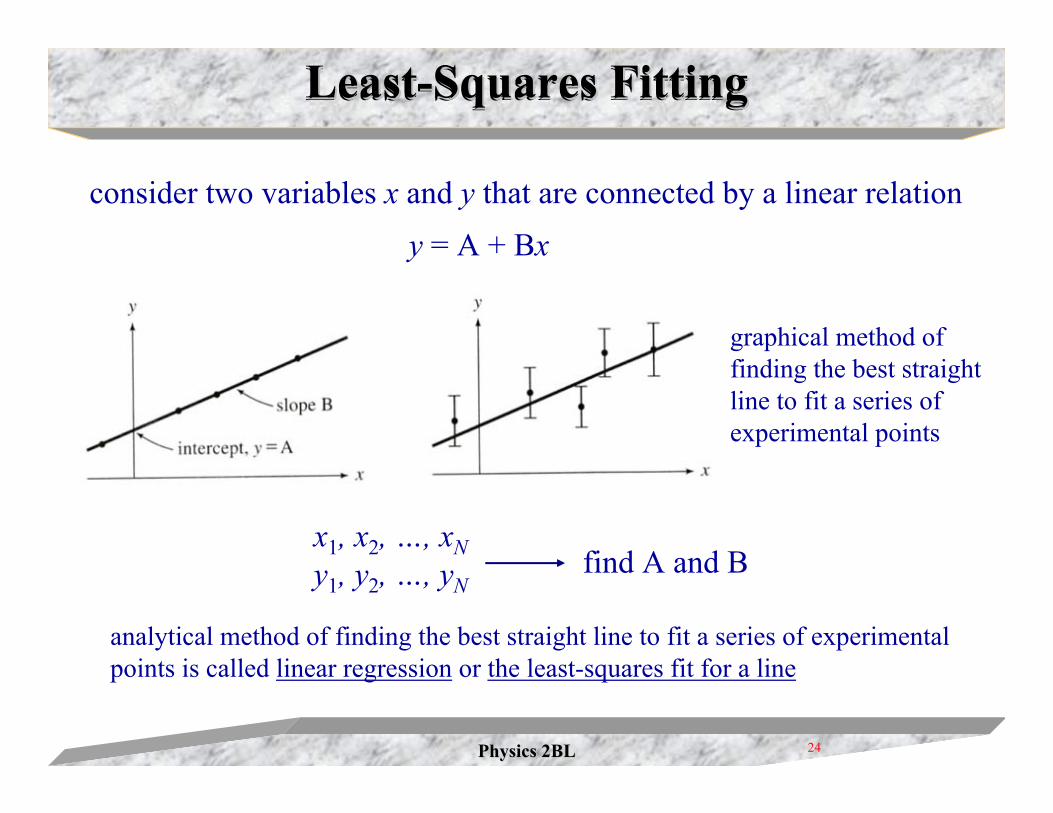
x1, x2, …, xNy1, y2, …, yN
consider two variables x and y that are connected by a linear relationy = A + Bx
find A and B
analytical method of finding the best straight line to fit a series of experimental points is called linear regression or the least-squares fit for a line
graphical method of finding the best straight line to fit a series of experimental points
Physics 2BLPhysics 2BL 25
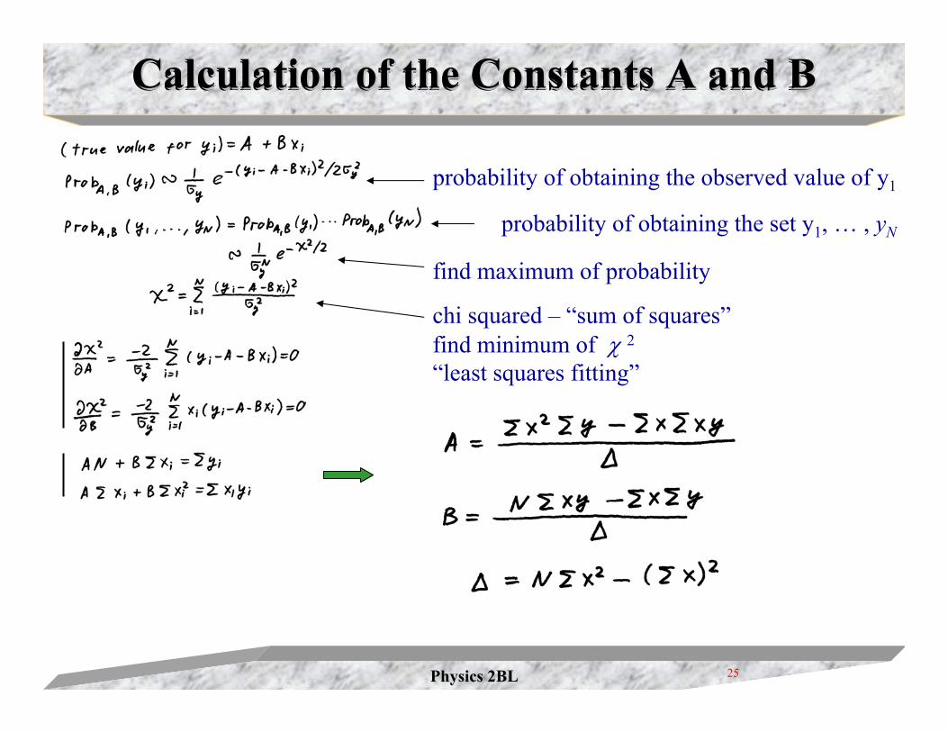
Calculation of the Constants A and BCalculation of the Constants A and BCalculation of the Constants A and B
probability of obtaining the observed value of y1
probability of obtaining the set y1, … , yN
find maximum of probability
chi squared – “sum of squares”find minimum of χ 2“least squares fitting”
Physics 2BLPhysics 2BL 26
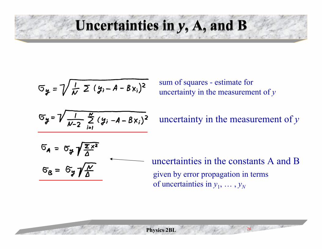
Uncertainties in y, A, and BUncertainties in Uncertainties in yy, A, and B, A, and B
uncertainty in the measurement of y
uncertainties in the constants A and B
sum of squares - estimate for uncertainty in the measurement of y
given by error propagation in terms of uncertainties in y1, … , yN
Physics 2BLPhysics 2BL 27
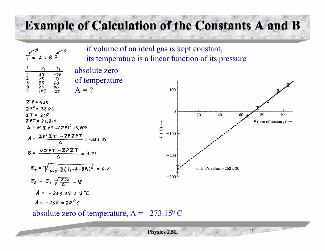
Example of Calculation of the Constants A and BExample of Calculation of the Constants A and BExample of Calculation of the Constants A and B
absolute zero of temperature, A = - 273.150 C
if volume of an ideal gas is kept constant, its temperature is a linear function of its pressure
absolute zero of temperatureA = ?
Physics 2BLPhysics 2BL 28
Covariance and CorrelationCovariance and CorrelationCovariance and Correlation
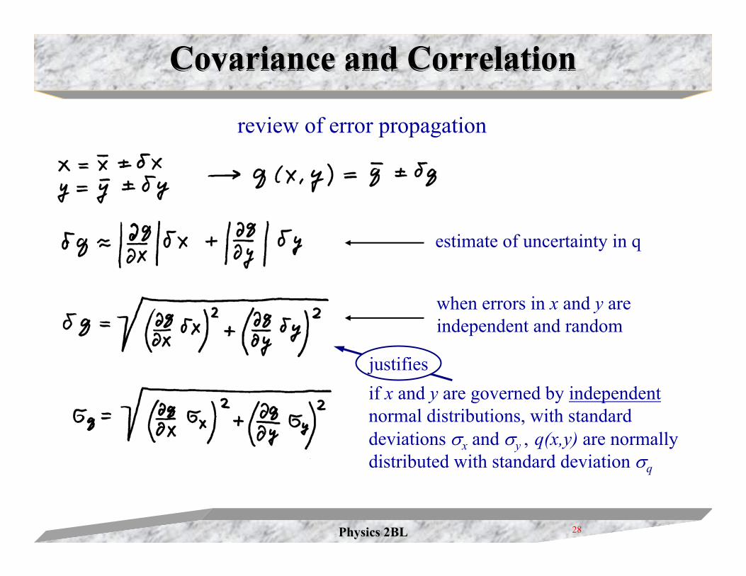
review of error propagation
when errors in x and y are independent and random
estimate of uncertainty in q
if x and y are governed by independent normal distributions, with standard deviations σx and σy , q(x,y) are normally distributed with standard deviation σq
justifies
Physics 2BLPhysics 2BL 29
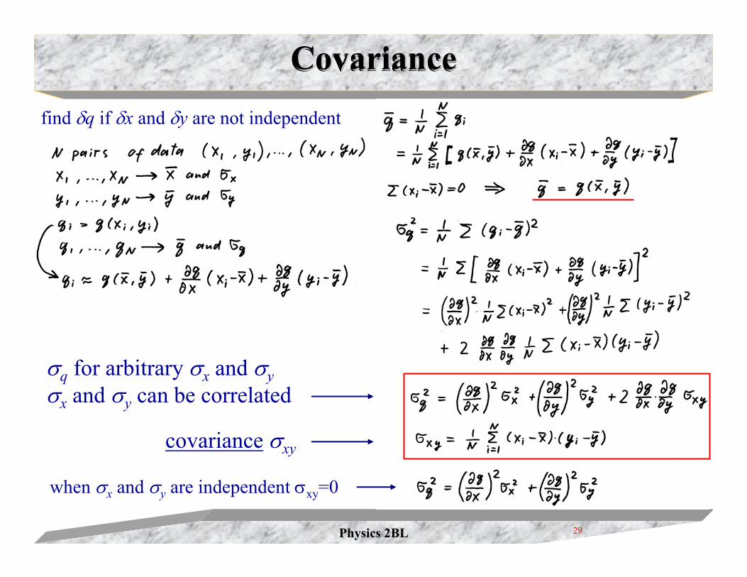
CovarianceCovarianceCovariancefind δq if δx and δy are not independent
σq for arbitrary σx and σyσx and σy can be correlated
covariance σxy
when σx and σy are independent σxy=0
Physics 2BLPhysics 2BL 30
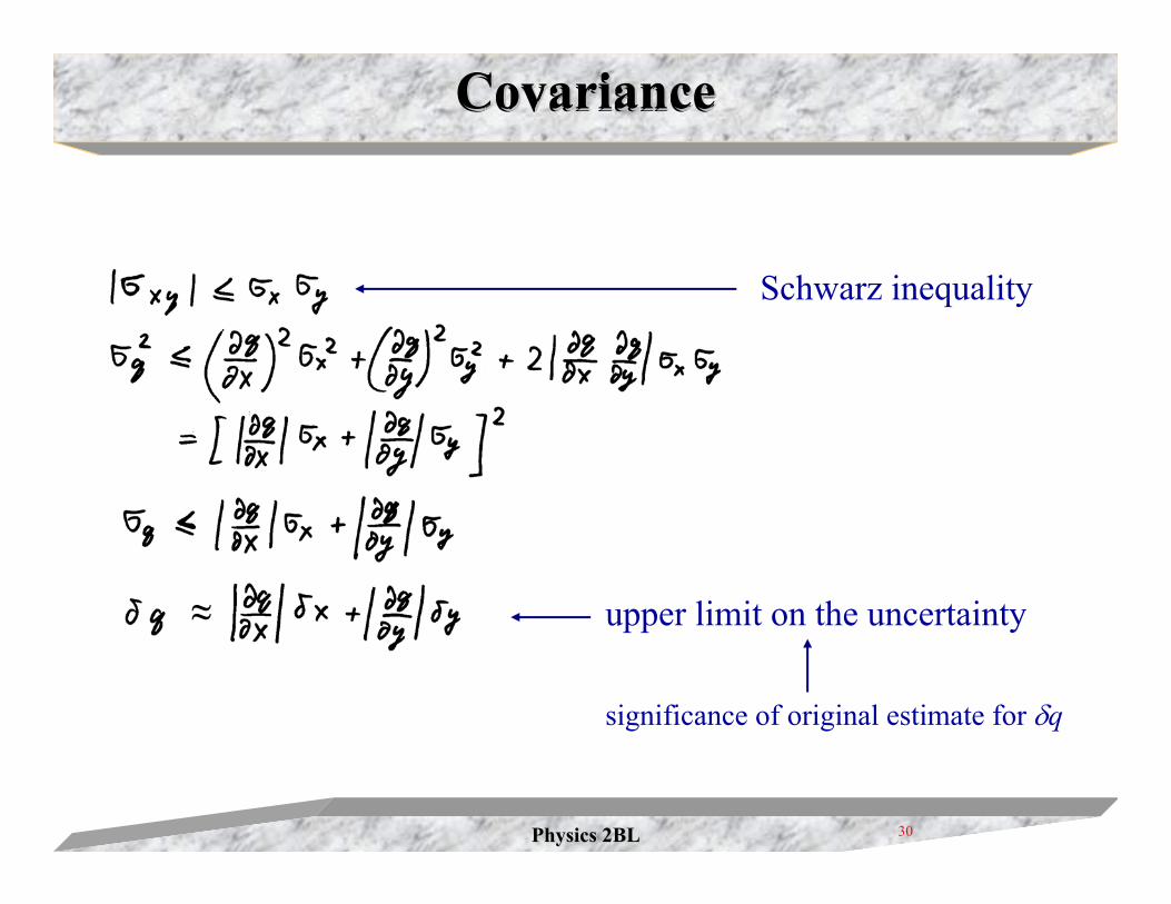
CovarianceCovarianceCovariance
Schwarz inequality
upper limit on the uncertainty≈
significance of original estimate for δq
Physics 2BLPhysics 2BL 31
Coefficient of Linear CorrelationCoefficient of Linear CorrelationCoefficient of Linear Correlation
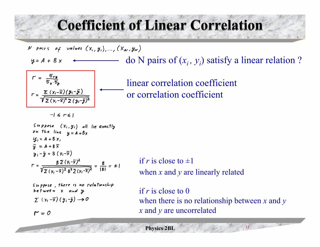
do N pairs of (xi , yi) satisfy a linear relation ?
linear correlation coefficientor correlation coefficient
if r is close to +1 when x and y are linearly related
if r is close to 0 when there is no relationship between x and yx and y are uncorrelated
_
Physics 2BLPhysics 2BL 32
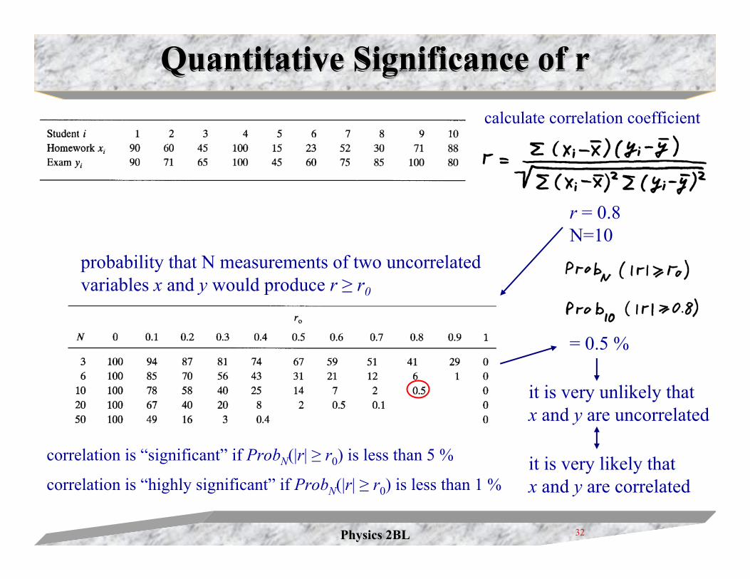
Quantitative Significance of rQuantitative Significance of rQuantitative Significance of r
r = 0.8N=10
probability that N measurements of two uncorrelated variables x and y would produce r ≥ r0
= 0.5 %
it is very unlikely that x and y are uncorrelated
it is very likely that x and y are correlated
calculate correlation coefficient
correlation is “significant” if ProbN(|r| ≥ r0) is less than 5 %
correlation is “highly significant” if ProbN(|r| ≥ r0) is less than 1 %
Physics 2BLPhysics 2BL 33
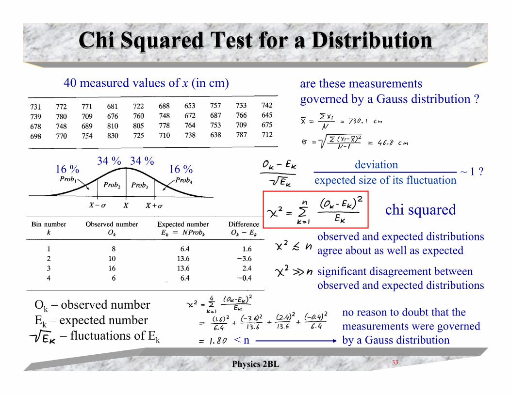
Chi Squared Test for a DistributionChi Squared Test for a DistributionChi Squared Test for a Distribution
40 measured values of x (in cm) are these measurements governed by a Gauss distribution ?
Ok – observed numberEk – expected number
– fluctuations of Ek
deviationexpected size of its fluctuation
16 % 16 %34 % 34 %
chi squared
~ 1 ?
observed and expected distributions agree about as well as expected
significant disagreement betweenobserved and expected distributions
no reason to doubt that the measurements were governed by a Gauss distribution< n
Physics 2BLPhysics 2BL 34
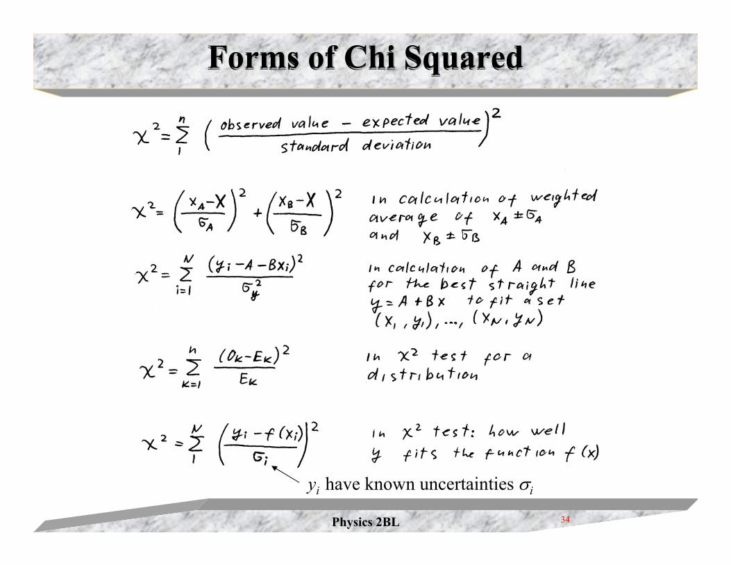
Forms of Chi SquaredForms of Chi SquaredForms of Chi Squared
yi have known uncertainties σi
Physics 2BLPhysics 2BL 35
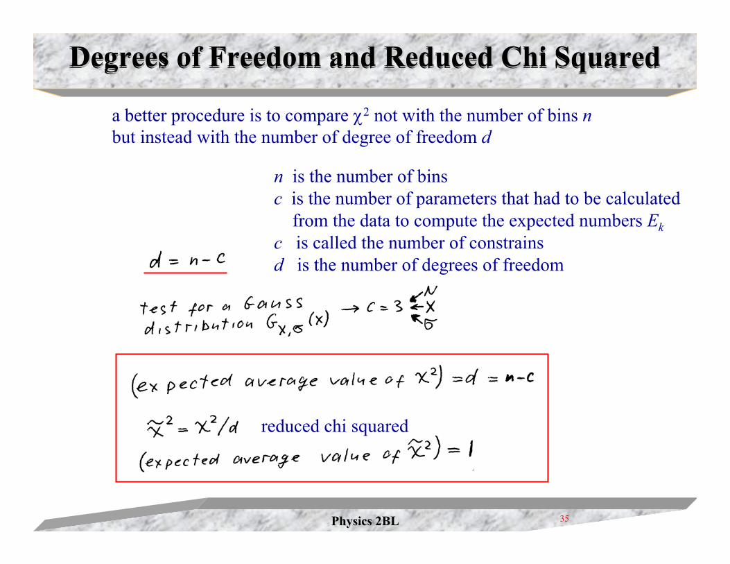
Degrees of Freedom and Reduced Chi SquaredDegrees of Freedom and Reduced Chi SquaredDegrees of Freedom and Reduced Chi Squared
n is the number of binsc is the number of parameters that had to be calculated
from the data to compute the expected numbers Ekc is called the number of constrainsd is the number of degrees of freedom
a better procedure is to compare χ2 not with the number of bins nbut instead with the number of degree of freedom d
reduced chi squared
Physics 2BLPhysics 2BL 36
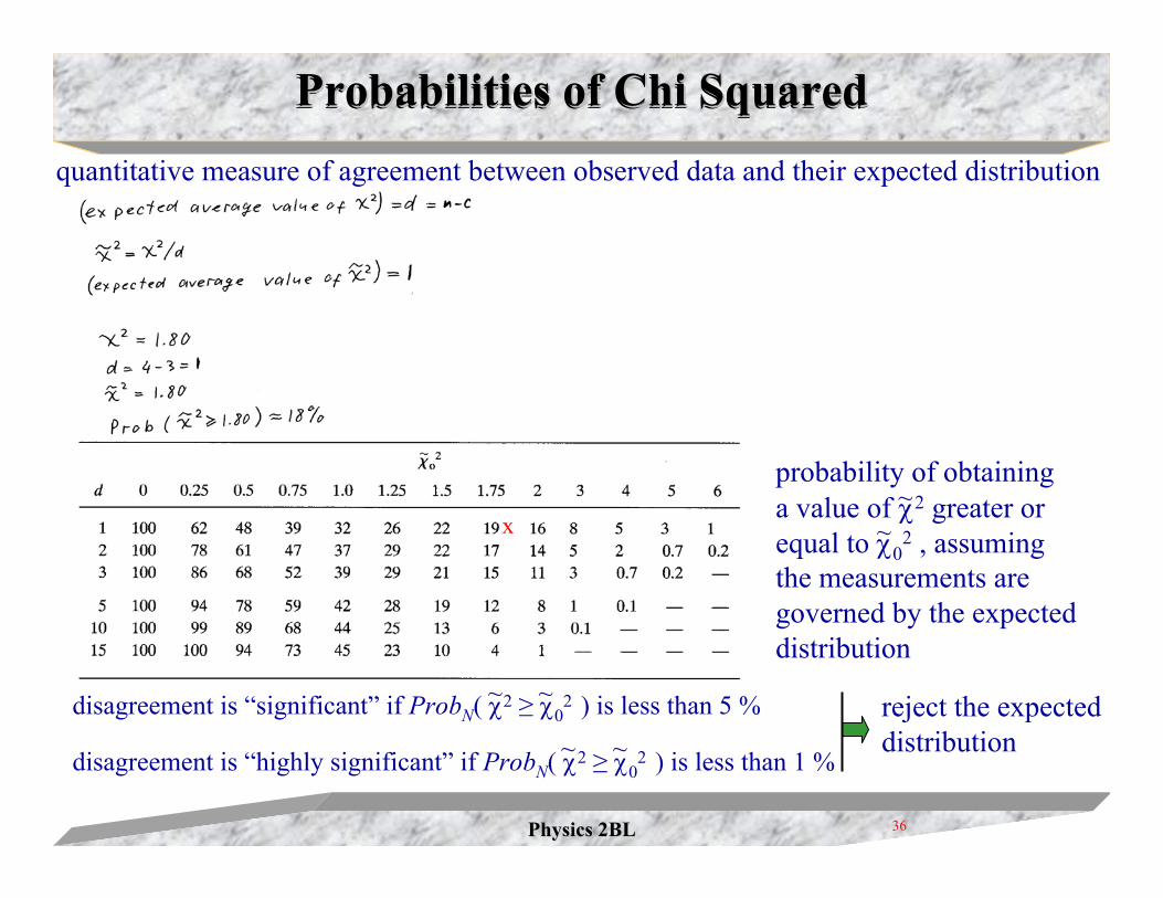
Probabilities of Chi SquaredProbabilities of Chi SquaredProbabilities of Chi Squaredquantitative measure of agreement between observed data and their expected distribution
x
disagreement is “significant” if ProbN( χ2 ≥ χ02 ) is less than 5 %
disagreement is “highly significant” if ProbN( χ2 ≥ χ02 ) is less than 1 %~~
~~
probability of obtaining a value of χ2 greater or equal to χ0
2 , assumingthe measurements are governed by the expected distribution
~~
reject the expected distribution