Computer Graphics III – Monte Carlo integration Direct...
61
Computer Graphics III – Monte Carlo integration Direct illumination Jaroslav Křivánek, MFF UK [email protected]
Transcript of Computer Graphics III – Monte Carlo integration Direct...
Computer Graphics III – Monte Carlo integration Direct illumination
Jaroslav Křivánek, MFF UK [email protected]

Entire the lecture in 5 slides
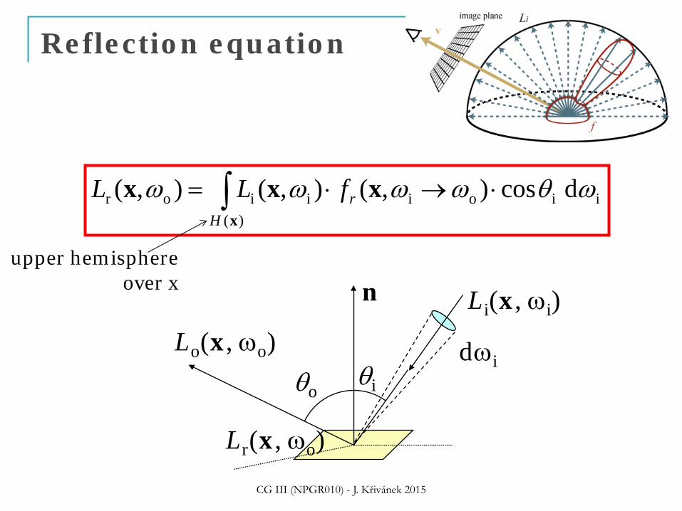
Reflection equation
∫ ⋅→⋅=)(
iioiiior dcos),(),(),(x
xxxH
rfLL ωθωωωω
dωi Lo(x, ωo)
θo
n Li(x, ωi)
θi
Lr(x, ωo)
upper hemisphere over x
CG III (NPGR010) - J. Křivánek 2015
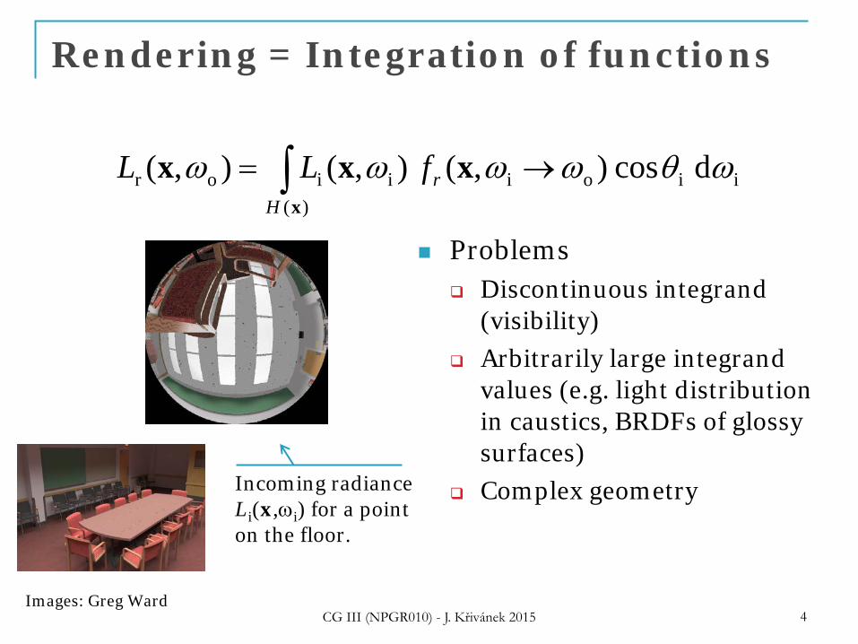
Rendering = Integration of functions
Problems Discontinuous integrand
(visibility) Arbitrarily large integrand
values (e.g. light distribution in caustics, BRDFs of glossy surfaces)
Complex geometry
CG III (NPGR010) - J. Křivánek 2015 4
∫ →=)(
iioiiior dcos),(),(),(x
xxxH
rfLL ωθωωωω
Incoming radiance Li(x,ωi) for a point on the floor.
Images: Greg Ward

Monte Carlo integration
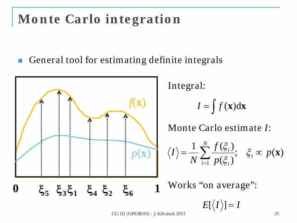
General tool for estimating definite integrals
ξ1
f(x)
0 1
p(x)
ξ2 ξ3 ξ4 ξ5 ξ6
∫= xx d)(fI
)(;)()(1
1xp
pf
NI i
N
i i
i ∝= ∑=
ξξξ
Integral:
Monte Carlo estimate I:
Works “on average”:
IIE =][CG III (NPGR010) - J. Křivánek 2015 5

Integral to be estimated:
PDF for cosine-proportional sampling:
MC estimator:
Application of MC to reflection eq: Estimator of reflected radiance
CG III (NPGR010) - J. Křivánek 2015 6
( )( )
∑
∑
=
=
→=
=
N
k,kr,k
N
k ,k
,kN
fLN
NF
1oiii
1 i
i
),(),(
pdfintegrand1
ωωωπ
ωω
xx
πθω cos)( =p
∫ →)(
iioiii dcos),(),(x
xxH
rfL ωθωωω

Variance => image noise
CG III (NPGR010) - J. Křivánek 2015 7

… and now the slow way

Digression: Numerical quadrature

Quadrature formulas for numerical integration
General formula in 1D:
f integrand (i.e. the integrated function) n quadrature order (i.e. number of integrand samples) xi node points (i.e. positions of the samples) f(xi) integrand values at node points wi quadrature weights
∑=
=n
iii xfwI
1)(ˆ
CG III (NPGR010) - J. Křivánek 2015 10
Quadrature formulas for numerical integration
Quadrature rules differ by the choice of node point positions xi and the weights wi
E.g. rectangle rule, trapezoidal rule, Simpson’s method,
Gauss quadrature, …
The samples (i.e. the node points) are placed deterministically
CG III (NPGR010) - J. Křivánek 2015 11
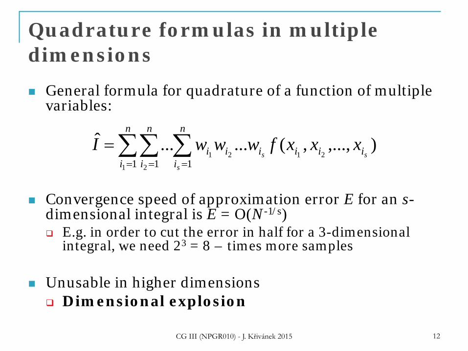
Quadrature formulas in multiple dimensions
General formula for quadrature of a function of multiple variables:
Convergence speed of approximation error E for an s-dimensional integral is E = O(N-1/s) E.g. in order to cut the error in half for a 3-dimensional
integral, we need 23 = 8 – times more samples
Unusable in higher dimensions Dimensional explosion
∑∑ ∑= = =
=n
i
n
i
n
iiiiiii
s
ssxxxfwwwI
1 1 11 2
2121),...,,(......ˆ
CG III (NPGR010) - J. Křivánek 2015 12
Quadrature formulas in multiple dimensions
Deterministic quadrature vs. Monte Carlo
In 1D deterministic better than Monte Carlo In 2D roughly equivalent From 3D, MC will always perform better
Remember, quadrature rules are NOT the Monte Carlo method
CG III (NPGR010) - J. Křivánek 2015 13

Monte Carlo

History of the Monte Carlo method
Atomic bomb development, Los Alamos 1940
John von Neumann, Stanislav Ulam, Nicholas Metropolis
Further development and practical applications from the early 50’s
CG III (NPGR010) - J. Křivánek 2015 15
Monte Carlo method
We simulate many random occurrences of the same type
of events, e.g.: Neutrons – emission, absorption, collisions with hydrogen
nuclei
Behavior of computer networks, traffic simulation.
Sociological and economical models – demography, inflation, insurance, etc.
CG III (NPGR010) - J. Křivánek 2015 16
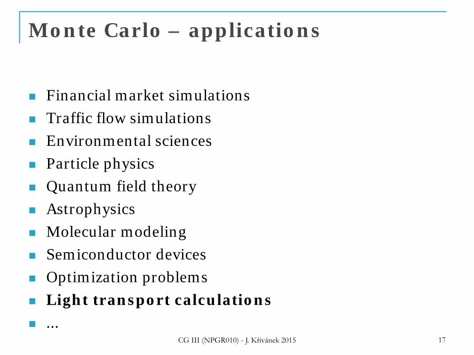
Monte Carlo – applications
Financial market simulations Traffic flow simulations Environmental sciences Particle physics Quantum field theory Astrophysics Molecular modeling Semiconductor devices Optimization problems Light transport calculations ...
CG III (NPGR010) - J. Křivánek 2015 17
CG III (NPGR010) - J. Křivánek 2015
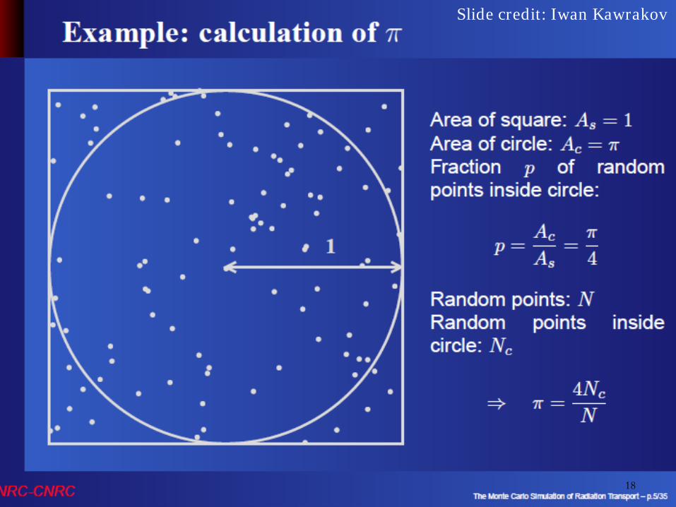
Slide credit: Iwan Kawrakov
18
CG III (NPGR010) - J. Křivánek 2015
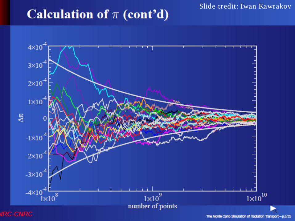
Slide credit: Iwan Kawrakov
19
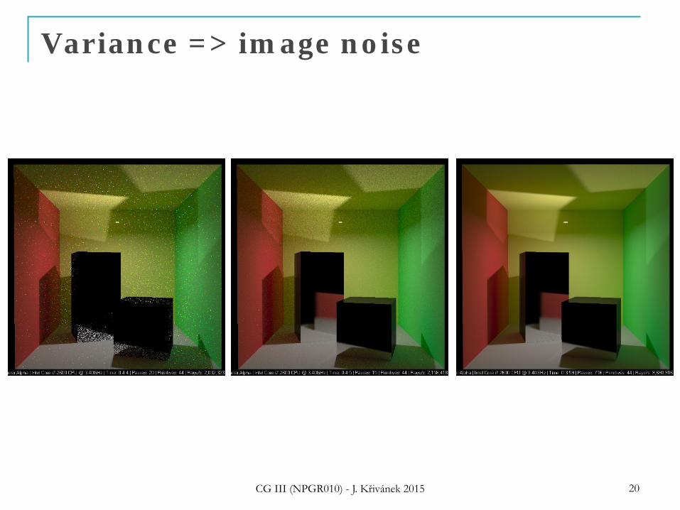
Variance => image noise
CG III (NPGR010) - J. Křivánek 2015 20
Monte Carlo integration
General tool for estimating definite integrals
ξ1
f(x)
0 1
p(x)
ξ2 ξ3 ξ4 ξ5 ξ6
∫= xx d)(fI
)(;)()(1
1xp
pf
NI i
N
i i
i ∝= ∑=
ξξξ
Integral:
Monte Carlo estimate I:
Works “on average”:
IIE =][CG III (NPGR010) - J. Křivánek 2015 21
Monte Carlo integration
Samples are placed randomly (or pseudo-randomly)
Convergence of standard error: std. dev. = O(N-1/2) Convergence speed independent of dimension Faster than classic quadrature rules for 3 and more
dimensions
Special methods for placing samples exist Quasi-Monte Carlo Faster asymptotic convergence than MC for “smooth”
functions
CG III (NPGR010) - J. Křivánek 2015 22
Monte Carlo integration
Pros Simple implementation Robust solution for complex integrands and integration
domains Effective for high-dimensional integrals
Cons
Relatively slow convergence – halving the standard error requires four times as many samples
In rendering: images contain noise that disappears slowly
CG III (NPGR010) - J. Křivánek 2015 23
Review – Random variables
Random variable
X … random variable
X assumes different values with different probability
Given by the probability distribution D X ∼ D
CG III (NPGR010) - J. Křivánek 2015 25
Discrete random variable
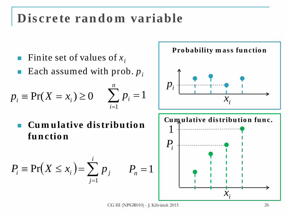
Finite set of values of xi Each assumed with prob. pi
Cumulative distribution function
CG III (NPGR010) - J. Křivánek 2015 26
0)Pr( ≥=≡ ii xXp ∑=
=n
iip
11
ipix
Probability mass function
( ) ∑=
=≤≡i
jjii pxXP
1Pr 1=nP
iP
ix
Cumulative distribution func. 1

Continuous random variable
Probability density function, pdf, p(x)
In 1D:
CG III (NPGR010) - J. Křivánek 2015 27
( ) xxpDXD
d)(Pr ∫=∈
( ) ∫=≤<b
attpbXa d)(Pr
Continuous random variable
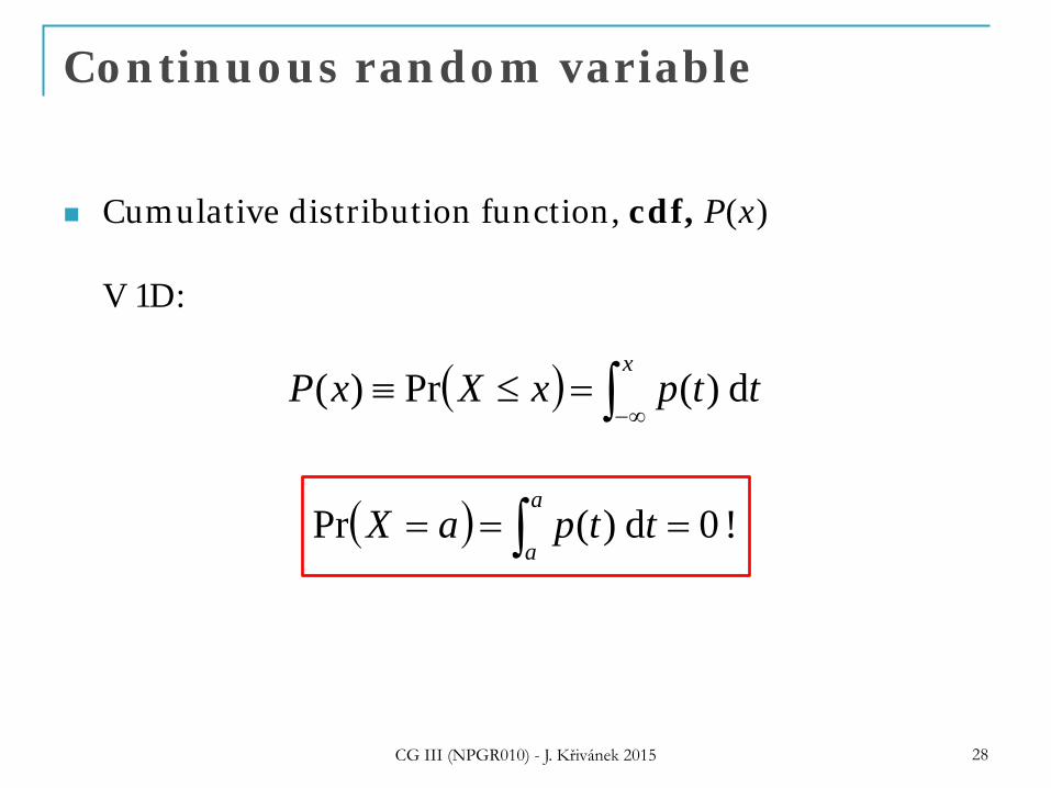
Cumulative distribution function, cdf, P(x) V 1D:
CG III (NPGR010) - J. Křivánek 2015 28
( ) ∫ ∞−=≤≡
xttpxXxP d)(Pr)(
( ) !0d)(Pr === ∫a
attpaX
Continuous random variable
CG III (NPGR010) - J. Křivánek 2015 29
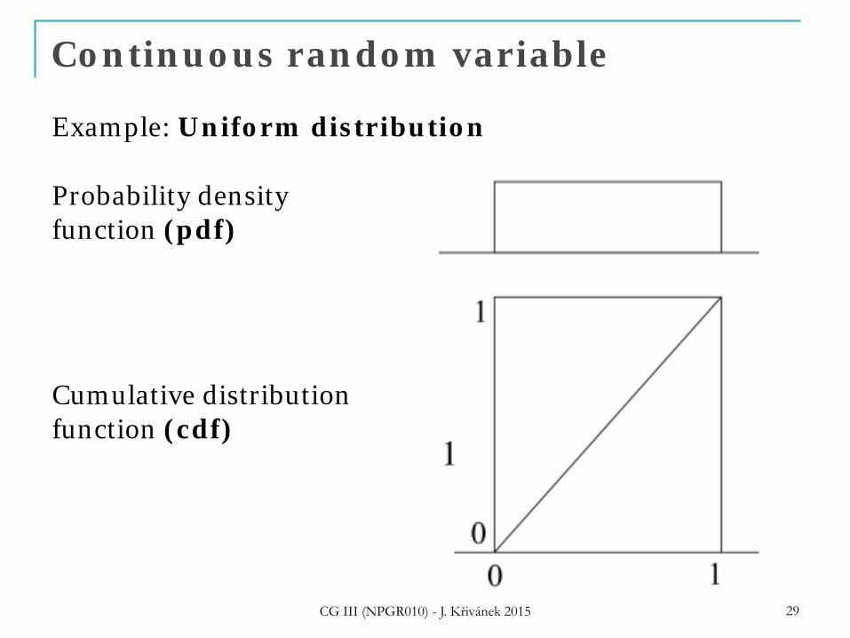
Example: Uniform distribution
Probability density function (pdf)
Cumulative distribution function (cdf)
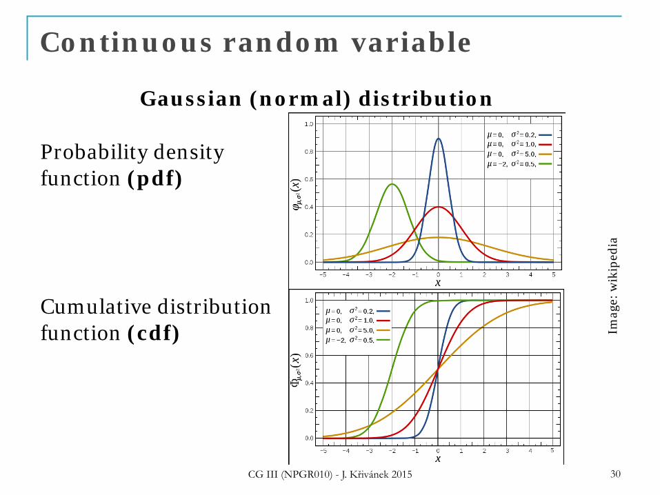
Continuous random variable
CG III (NPGR010) - J. Křivánek 2015 30
Imag
e: w
ikip
edia
Gaussian (normal) distribution
Probability density function (pdf)
Cumulative distribution function (cdf)
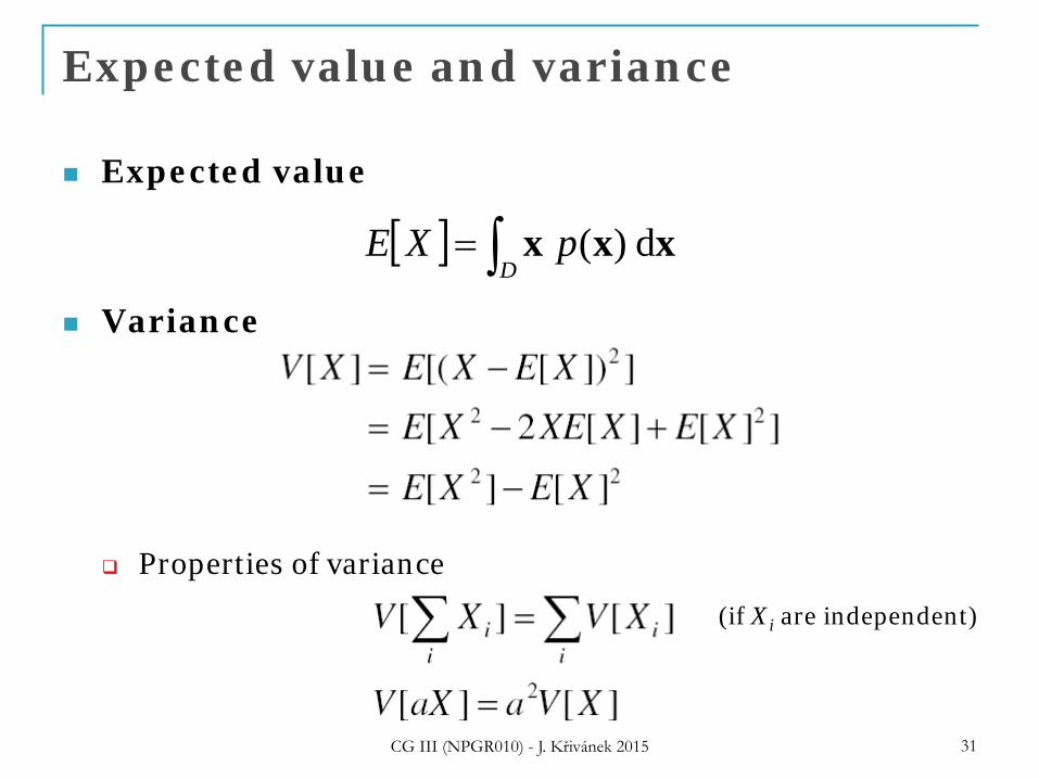
Expected value and variance
Expected value
Variance
Properties of variance
[ ] ∫=D
pXE xxx d)(
(if Xi are independent)
CG III (NPGR010) - J. Křivánek 2015 31
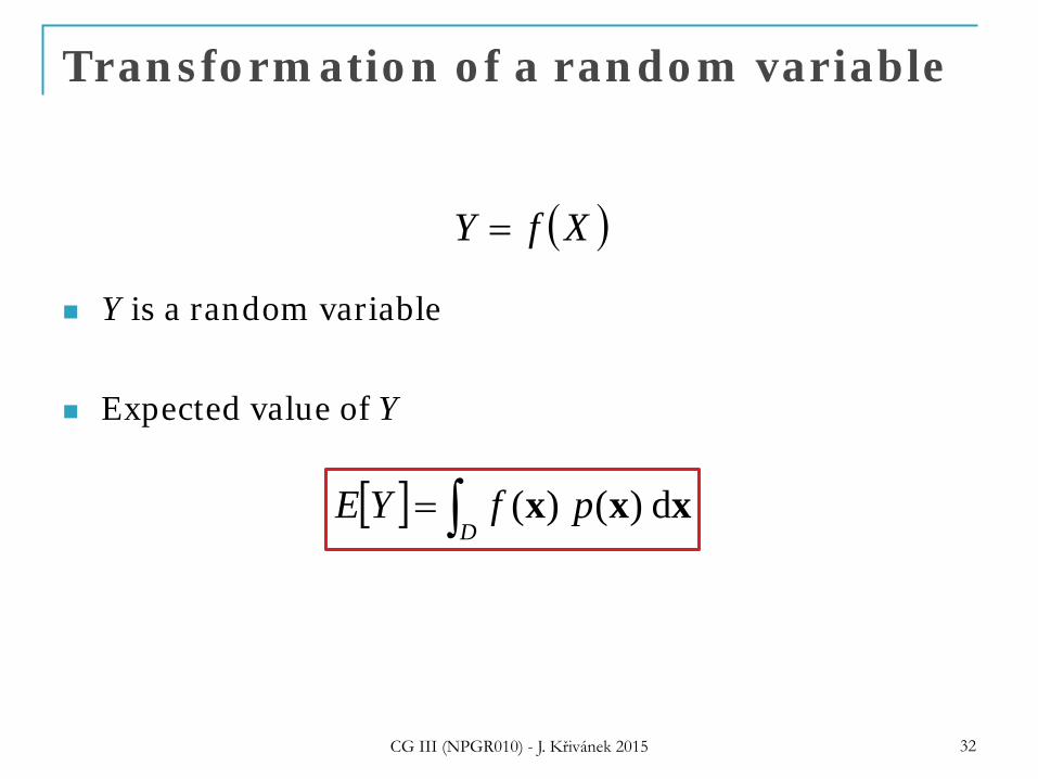
Transformation of a random variable
Y is a random variable
Expected value of Y
CG III (NPGR010) - J. Křivánek 2015 32
( )XfY =
[ ] ∫=D
pfYE xxx d)()(

Monte Carlo integration

Monte Carlo integration
General tool for estimating definite integrals
ξ1
f(x)
0 1
p(x)
ξ2 ξ3 ξ4 ξ5 ξ6
∫= xx d)(fI
)(;)()(1
1xp
pf
NI i
N
i i
i ∝= ∑=
ξξξ
Integral:
Monte Carlo estimate I:
Works “on average”:
IIE =][CG III (NPGR010) - J. Křivánek 2015 34
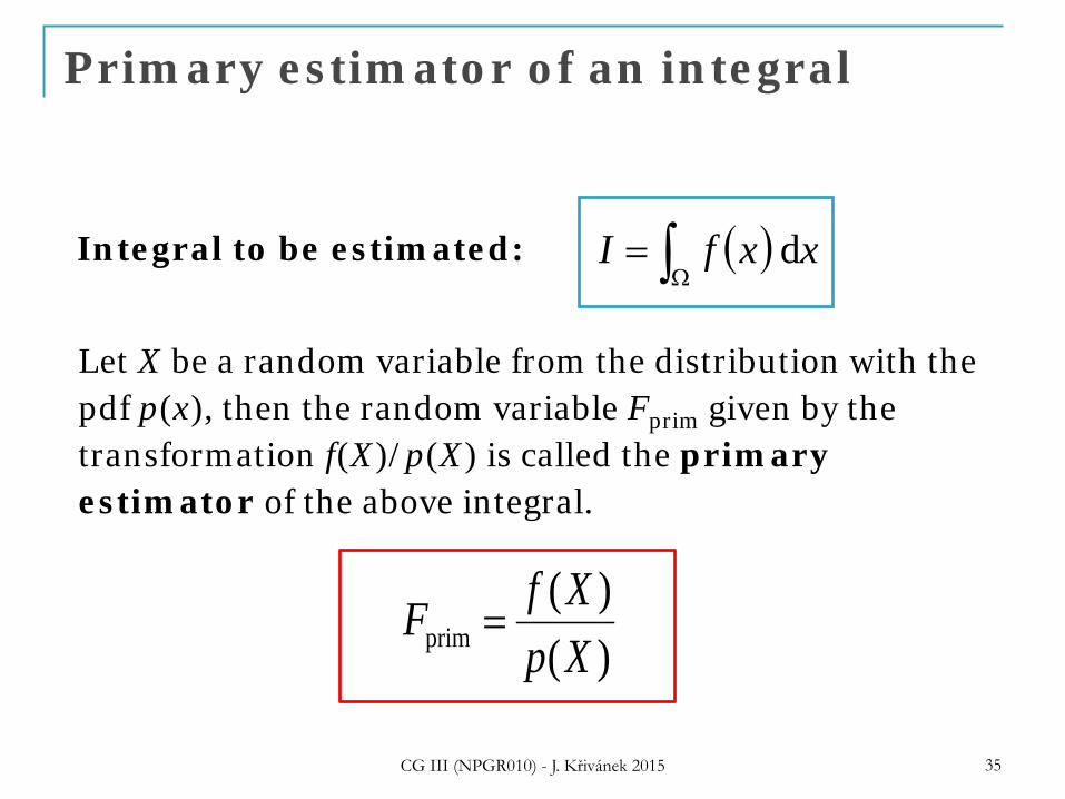
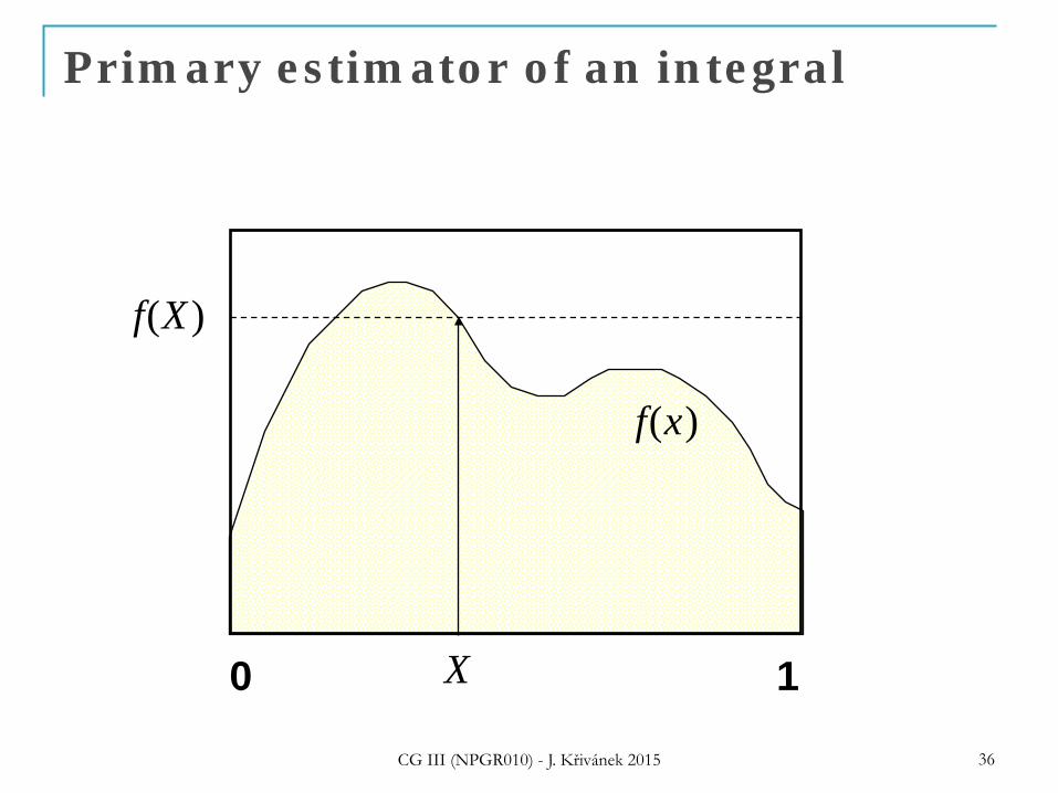
( )∫Ω= xxfI dIntegral to be estimated:
Let X be a random variable from the distribution with the pdf p(x), then the random variable Fprim given by the transformation f(X)/p(X) is called the primary estimator of the above integral.
)()(
prim XpXfF =
CG III (NPGR010) - J. Křivánek 2015 35
Primary estimator of an integral
Primary estimator of an integral
X
f(x)
f(X)
0 1
CG III (NPGR010) - J. Křivánek 2015 36
Estimator vs. estimate
Estimator is a random variable It is defined though a transformation of another random
variable
Estimate is a concrete realization (outcome) of the estimator
No need to worry: the above distinction is important for proving theorems but less important in practice
CG III (NPGR010) - J. Křivánek 2015 37
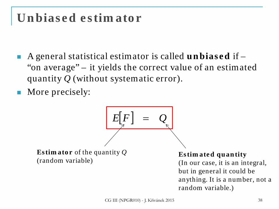
Unbiased estimator
A general statistical estimator is called unbiased if – “on average” – it yields the correct value of an estimated quantity Q (without systematic error).
More precisely:
CG III (NPGR010) - J. Křivánek 2015 38
[ ] QFE =
Estimated quantity (In our case, it is an integral, but in general it could be anything. It is a number, not a random variable.)
Estimator of the quantity Q (random variable)
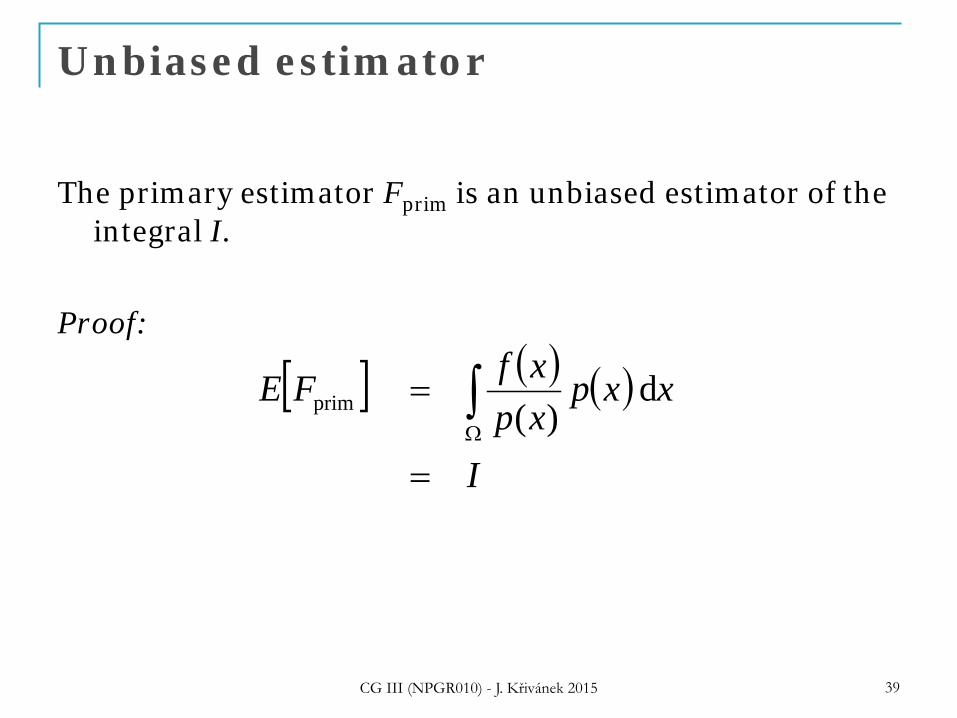
Unbiased estimator
The primary estimator Fprim is an unbiased estimator of the integral I.
Proof:
CG III (NPGR010) - J. Křivánek 2015 39
[ ] ( ) ( )
I
xxpxpxfFE
=
= ∫Ω
d)(prim
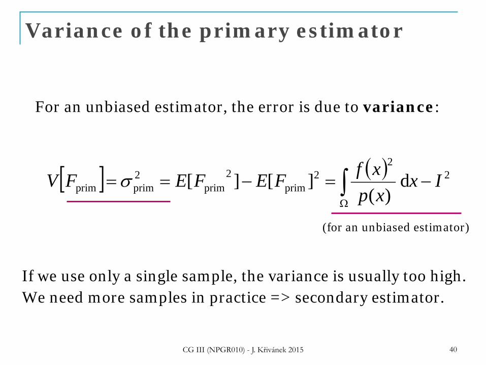
Variance of the primary estimator
[ ] ( ) 22
2prim
2prim
2primprim d
)(][][ Ix
xpxfFEFEFV −=−== ∫
Ω
σ
For an unbiased estimator, the error is due to variance:
If we use only a single sample, the variance is usually too high. We need more samples in practice => secondary estimator.
(for an unbiased estimator)
CG III (NPGR010) - J. Křivánek 2015 40
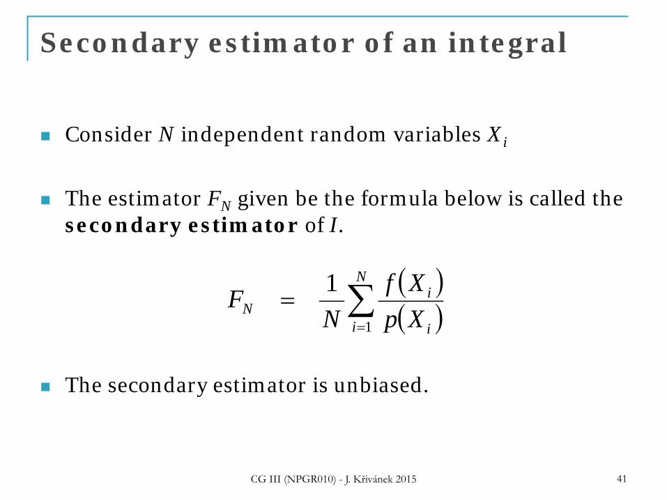
Secondary estimator of an integral
Consider N independent random variables Xi
The estimator FN given be the formula below is called the secondary estimator of I.
The secondary estimator is unbiased.
CG III (NPGR010) - J. Křivánek 2015 41
( )( )∑
=
=N
i i
iN Xp
XfN
F1
1
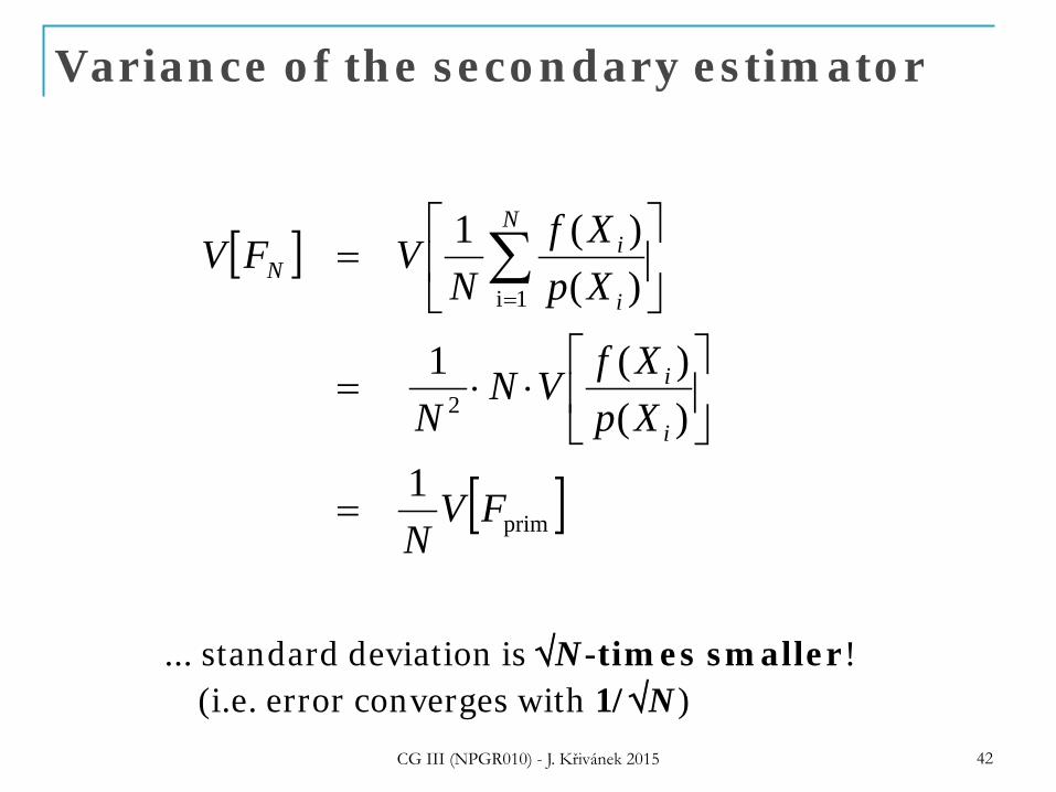
Variance of the secondary estimator
[ ]
[ ]prim
2
1i
1)()(1
)()(1
FVN
XpXfVN
N
XpXf
NVFV
i
i
N
i
iN
=
⋅⋅=
= ∑
=
... standard deviation is √N-times smaller! (i.e. error converges with 1/√N)
CG III (NPGR010) - J. Křivánek 2015 42

Properties of estimators

Unbiased estimator
A general statistical estimator is called unbiased if – “on average” – it yields the correct value of an estimated quantity Q (without systematic error).
More precisely:
CG III (NPGR010) - J. Křivánek 2015 44
[ ] QFE =
Estimated quantity (In our case, it is an integral, but in general it could be anything. It is a number, not a random variable.)
Estimator of the quantity Q (random variable)
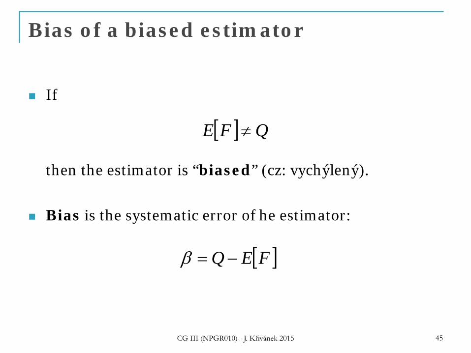
Bias of a biased estimator
If then the estimator is “biased” (cz: vychýlený).
Bias is the systematic error of he estimator:
CG III (NPGR010) - J. Křivánek 2015 45
[ ] QFE ≠
[ ]FEQ −=β
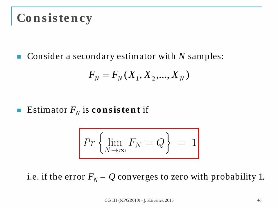
Consistency
Consider a secondary estimator with N samples:
Estimator FN is consistent if i.e. if the error FN – Q converges to zero with probability 1.
CG III (NPGR010) - J. Křivánek 2015 46
),...,,( 21 NNN XXXFF =
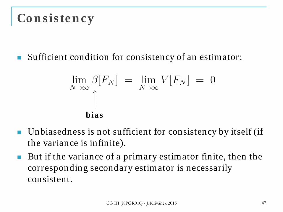
Consistency
Sufficient condition for consistency of an estimator:
Unbiasedness is not sufficient for consistency by itself (if
the variance is infinite). But if the variance of a primary estimator finite, then the
corresponding secondary estimator is necessarily consistent.
CG III (NPGR010) - J. Křivánek 2015 47
bias
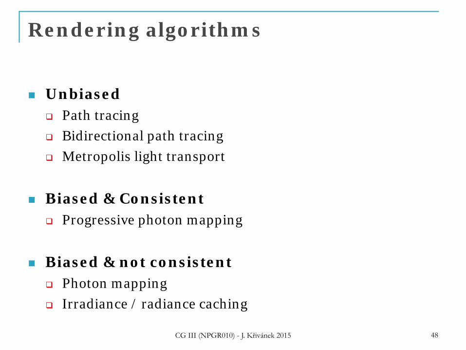
Rendering algorithms
Unbiased Path tracing Bidirectional path tracing Metropolis light transport
Biased & Consistent
Progressive photon mapping
Biased & not consistent Photon mapping Irradiance / radiance caching
CG III (NPGR010) - J. Křivánek 2015 48
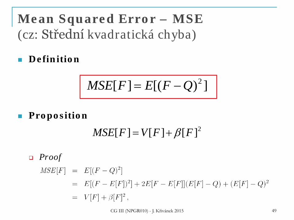
Mean Squared Error – MSE (cz: Střední kvadratická chyba)
Definition
Proposition
Proof
CG III (NPGR010) - J. Křivánek 2015 49
])[(][ 2QFEFMSE −=
2][][][ FFVFMSE β+=

Mean Squared Error – MSE (cz: Střední kvadratická chyba)
If the estimator F is unbiased, then i.e. for an unbiased estimator, it is much easier to estimate the error, because it can be estimated directly from the samples Yi = f(Xi) / p(Xi).
Unbiased estimator of variance
CG III (NPGR010) - J. Křivánek 2015 50
][][ FVFMSE =
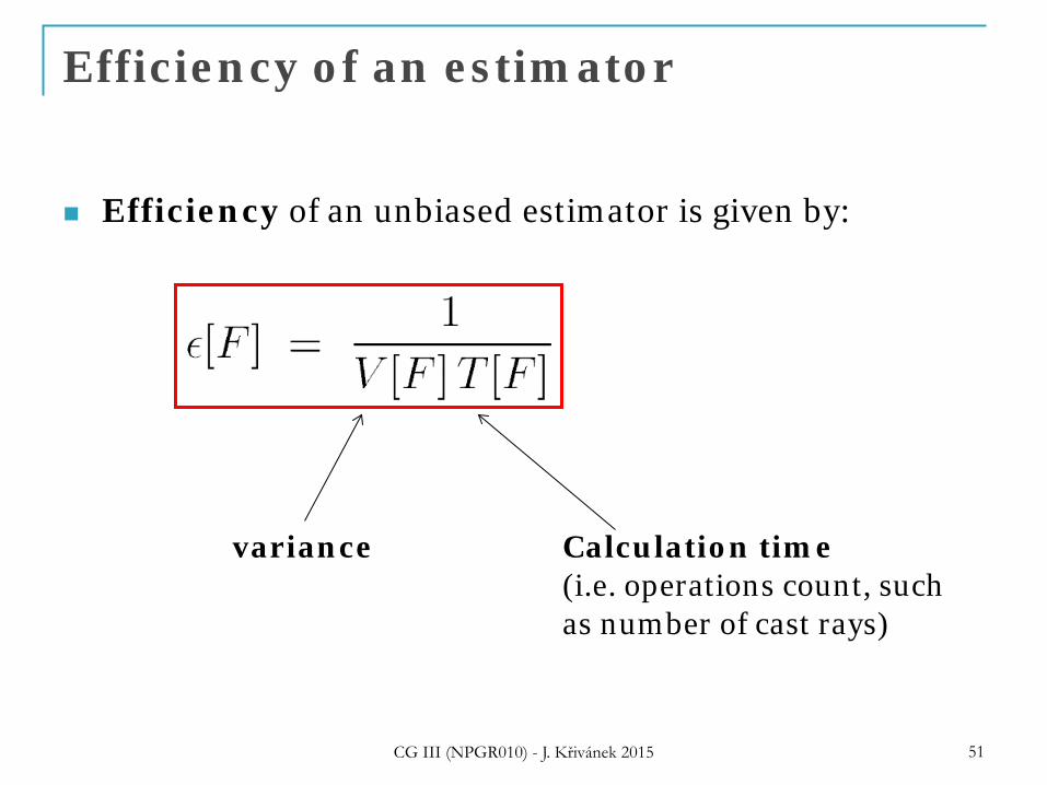
Efficiency of an estimator
Efficiency of an unbiased estimator is given by:
CG III (NPGR010) - J. Křivánek 2015 51
variance Calculation time (i.e. operations count, such as number of cast rays)
MC estimators for illumination calculation

PDF for uniform sampling:
Estimator:
Irradiance estimator – uniform sampling
CG III (NPGR010) - J. Křivánek 2015 53
∫ ⋅=)(
iiii dcos),()(x
xxH
LE ωθωπ
ω21)( =p
( )( )
∑
∑
=
=
⋅=
=
N
k,kk
N
k k
kN
LN
pf
NF
1ii,i
1 i,
i,
cos),(2
1
θωπ
ωω
x
Integral to be estimated:
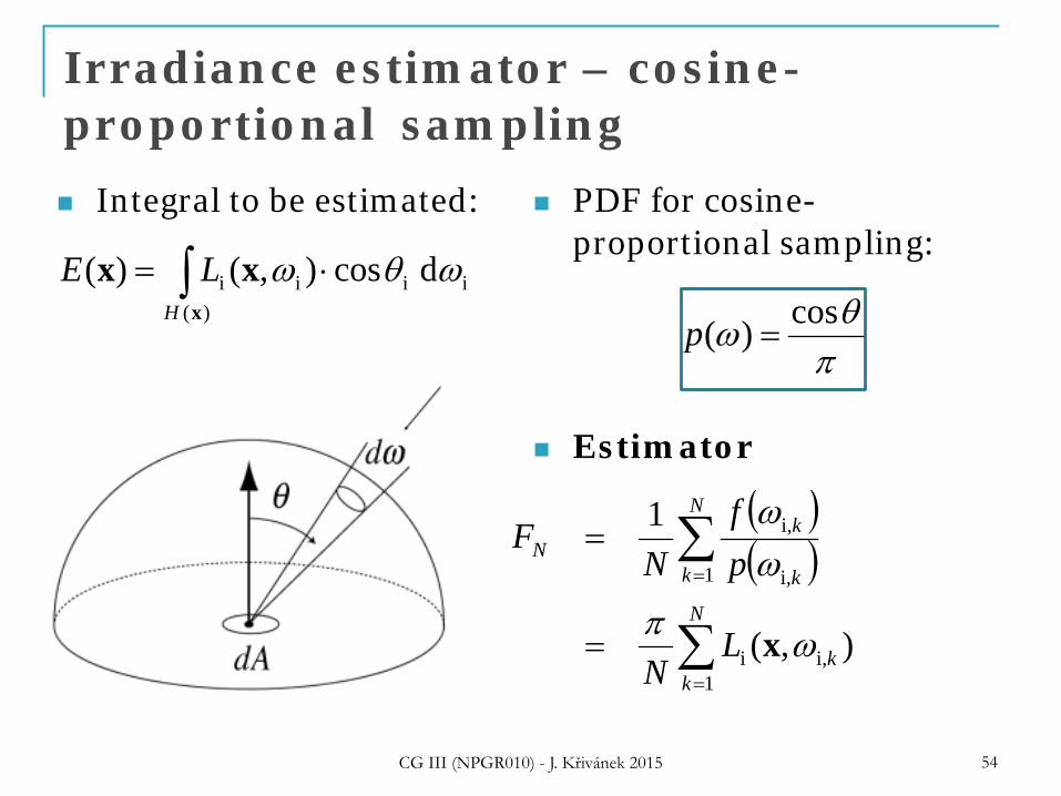
Irradiance estimator – cosine-proportional sampling
CG III (NPGR010) - J. Křivánek 2015 54
( )( )
∑
∑
=
=
=
=
N
k,k
N
k ,k
,kN
LN
pf
NF
1ii
1 i
i
),(
1
ωπ
ωω
x
PDF for cosine-proportional sampling:
Estimator
Integral to be estimated:
∫ ⋅=)(
iiii dcos),()(x
xxH
LE ωθω
πθω cos)( =p
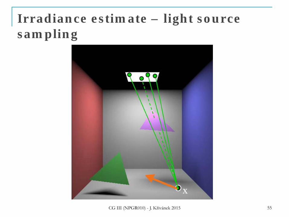
Irradiance estimate – light source sampling
CG III (NPGR010) - J. Křivánek 2015 55
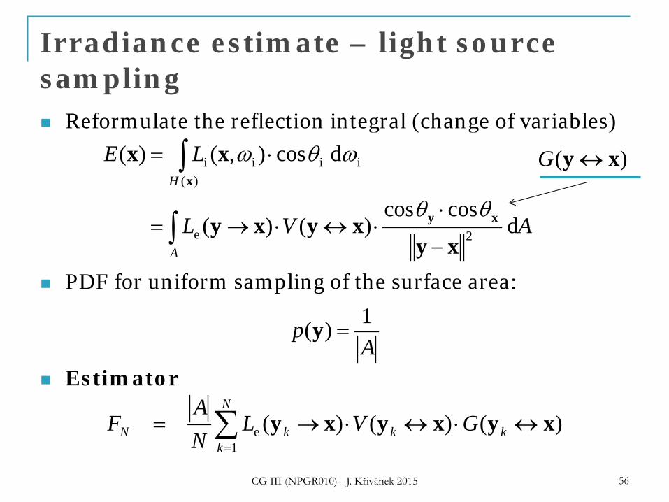
Irradiance estimate – light source sampling Reformulate the reflection integral (change of variables)
PDF for uniform sampling of the surface area:
Estimator
CG III (NPGR010) - J. Křivánek 2015 56
∫
∫
−
⋅⋅↔⋅→=
⋅=
A
H
AVL
LE
dcoscos
)()(
dcos),()(
2e
)(iiii
xyxyxy
xx
xy
x
θθ
ωθω )( xy ↔G
Ap 1)( =y
∑=
↔⋅↔⋅→=N
kkkkN GVL
NA
F1
e )()()( xyxyxy
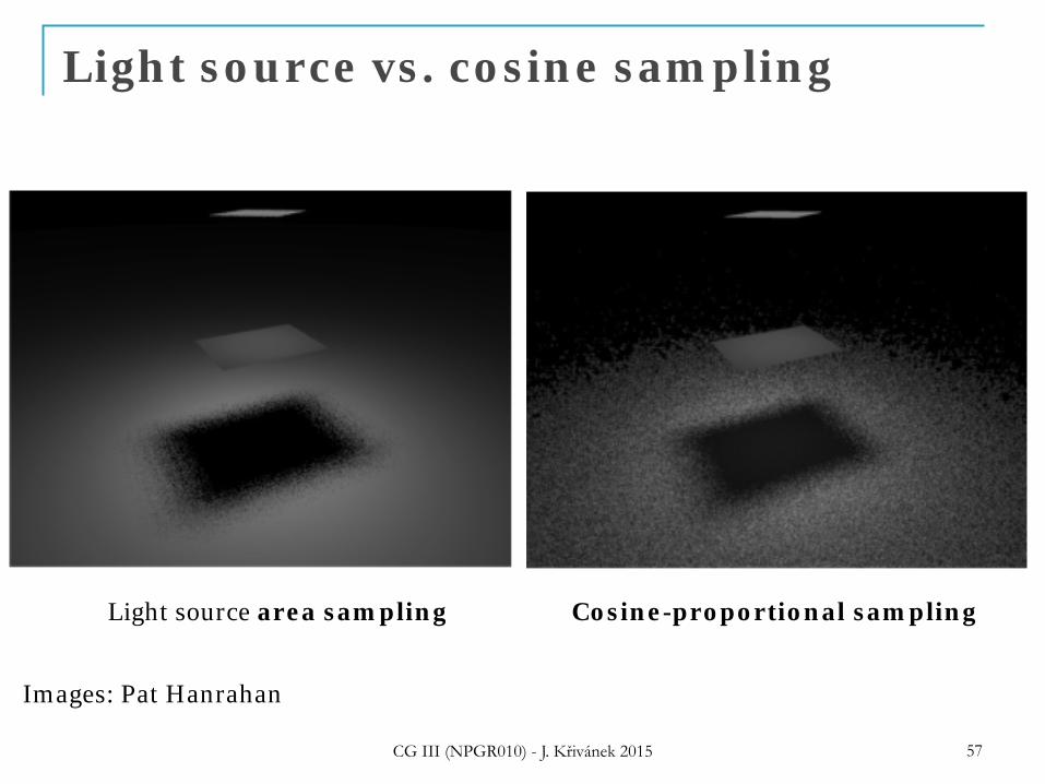
Light source vs. cosine sampling
CG III (NPGR010) - J. Křivánek 2015 57
Light source area sampling Cosine-proportional sampling
Images: Pat Hanrahan
CG III (NPGR010) - J. Křivánek 2015 58
CG III (NPGR010) - J. Křivánek 2015 59
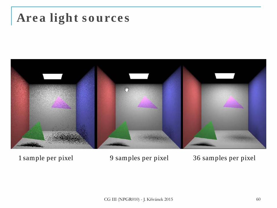
Area light sources
1 sample per pixel 9 samples per pixel 36 samples per pixel
CG III (NPGR010) - J. Křivánek 2015 60
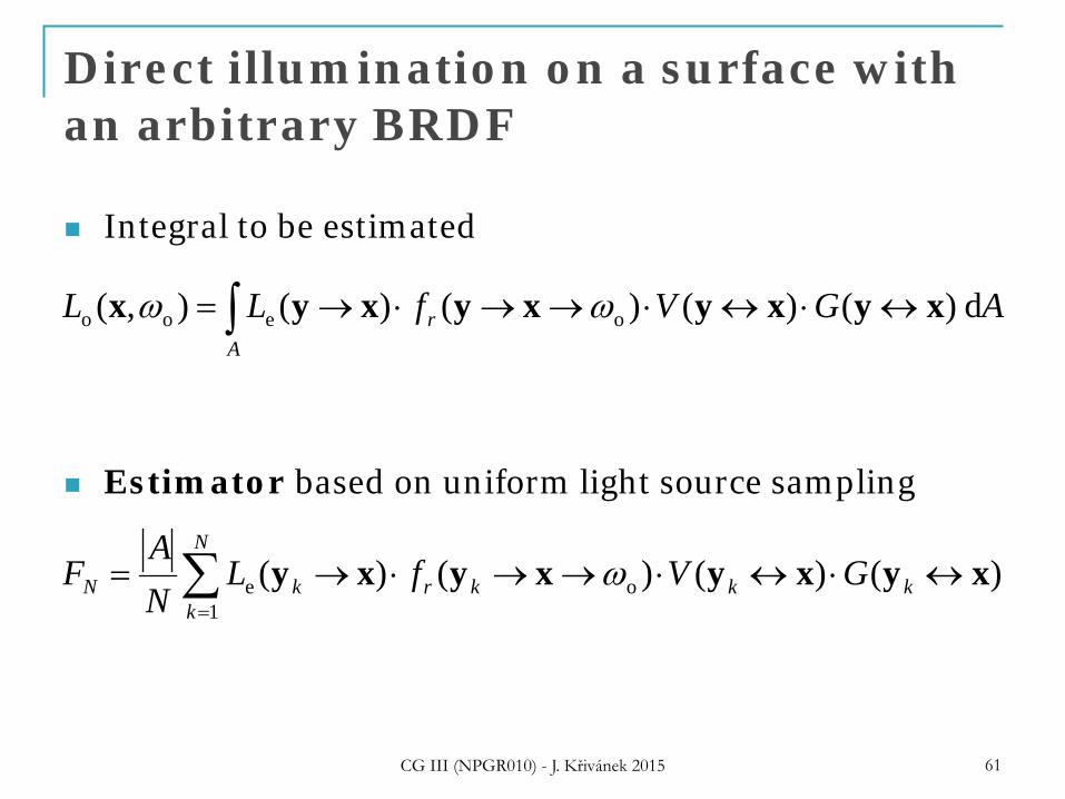
Direct illumination on a surface with an arbitrary BRDF
Integral to be estimated
Estimator based on uniform light source sampling
CG III (NPGR010) - J. Křivánek 2015 61
∫ ↔⋅↔⋅→→⋅→=A
r AGVfLL d)()()()(),( oeoo xyxyxyxyx ωω
∑=
↔⋅↔⋅→→⋅→=N
kkkkrkN GVfL
NA
F1
oe )()()()( xyxyxyxy ω