
Princeton University Diffusion of Networking Technologies Sharon Goldberg Boston University BIRS...
40
Princeton University Diffusion of Networking Technologies Sharon Goldberg Boston University BIRS workshop 2013 Zhenming Liu Princeton University ISP
Transcript of Princeton University Diffusion of Networking Technologies Sharon Goldberg Boston University BIRS...
Princeton University
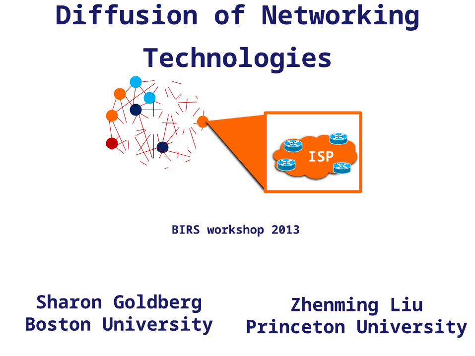
Diffusion of Networking
Technologies
Sharon GoldbergBoston University
BIRS workshop 2013
Zhenming LiuPrinceton University
ISP
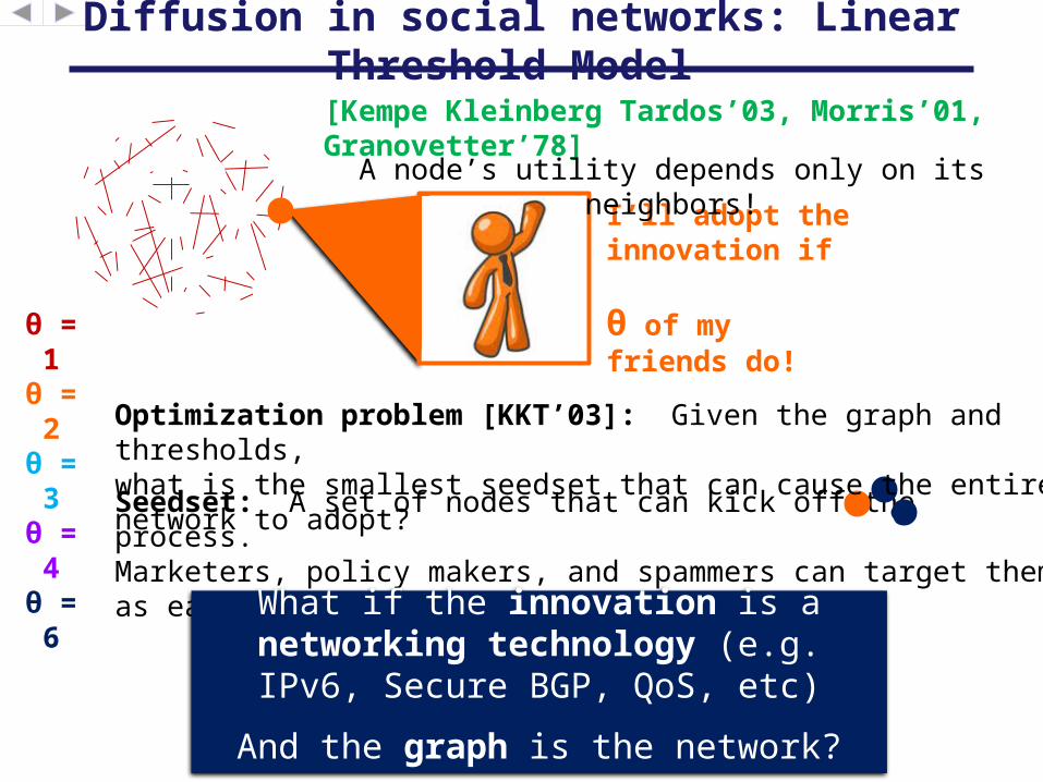
Seedset: A set of nodes that can kick off the process.Marketers, policy makers, and spammers can target them as early adopters!
I’ll adopt the innovation if θ of my friends do!
Diffusion in social networks: Linear Threshold Model
What if the innovation is a networking technology (e.g. IPv6,
Secure BGP, QoS, etc)
And the graph is the network?
[Kempe Kleinberg Tardos’03, Morris’01, Granovetter’78]
θ = 1
θ = 2
θ = 3
θ = 4
θ = 6
Optimization problem [KKT’03]: Given the graph and thresholds,what is the smallest seedset that can cause the entire network to adopt?
A node’s utility depends only on its neighbors!
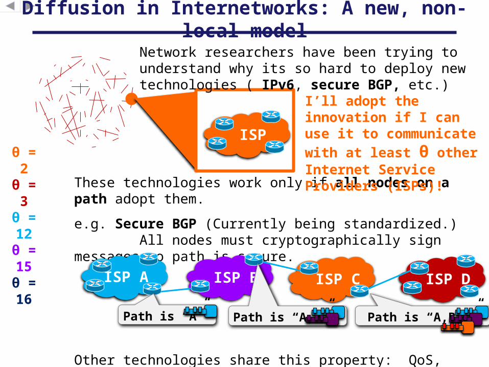
These technologies work only if all nodes on a path adopt them.
e.g. Secure BGP (Currently being standardized.) All nodes must cryptographically sign messages so path is secure.
Other technologies share this property: QoS, fault localization, IPv6, …
Diffusion in Internetworks: A new, non-local model
I’ll adopt the innovation if I can use it to communicate with at least θ other Internet Service Providers (ISPs)!
ISP
Network researchers have been trying to understand why its so hard to deploy new technologies ( IPv6, secure BGP, etc.)
ISP B ISP A ISP C ISP D
Path is “A” Path is “A,B” Path is “A,B,C”
θ = 2
θ = 3
θ = 12θ = 15θ = 16
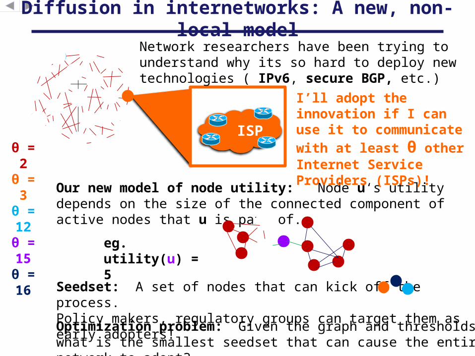
Diffusion in internetworks: A new, non-local model
θ = 2
θ = 3
θ = 12θ = 15θ = 16
Our new model of node utility: Node u‘s utility depends on the size of the connected component of active nodes that u is part of.
Optimization problem: Given the graph and thresholds,what is the smallest seedset that can cause the entire network to adopt?
ISP
Network researchers have been trying to understand why its so hard to deploy new technologies ( IPv6, secure BGP, etc.)
Seedset: A set of nodes that can kick off the process.Policy makers, regulatory groups can target them as early adopters!
I’ll adopt the innovation if I can use it to communicate with at least θ other Internet Service Providers (ISPs)!
eg. utility(u) = 5
Interpretation of the model
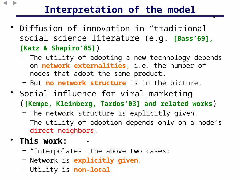
• Diffusion of innovation in “traditional” social science literature (e.g. [Bass’69], [Katz & Shapiro’85])– The utility of adopting a new technology depends on
network externalities, i.e. the number of nodes that adopt the same product.
– But no network structure is in the picture. • Social influence for viral marketing ([Kempe,
Kleinberg, Tardos’03] and related works)– The network structure is explicitly given. – The utility of adoption depends only on a node’s direct
neighbors. • This work:
– “Interpolates” the above two cases:– Network is explicitly given. – Utility is non-local.
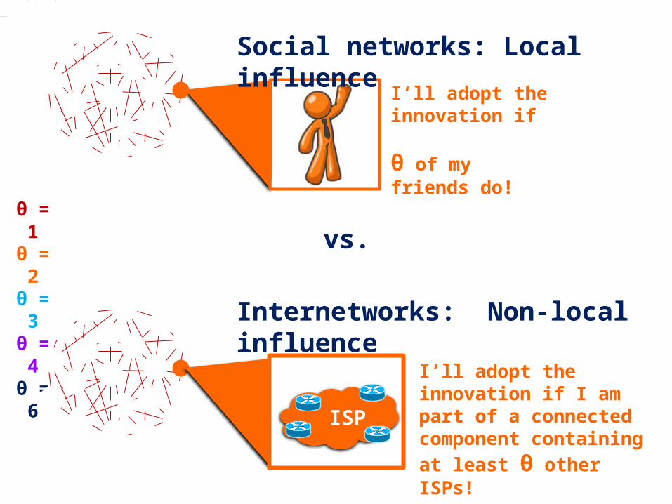
I’ll adopt the innovation if θ of my friends do!
Social networks: Local influence
θ = 1
θ = 2
θ = 3
θ = 4
θ = 6
I’ll adopt the innovation if I am part of a connected component containing at least θ other ISPs!
ISP
Internetworks: Non-local influence
vs.
Social networks vs Internetworks
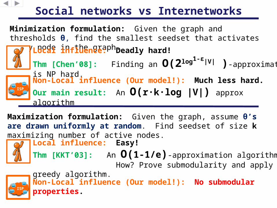
Minimization formulation: Given the graph and thresholds θ, find the smallest seedset that activates every node in the graph.
Local influence: Deadly hard!
Thm [Chen’08]: Finding an O(2log1-ε|V| )-approximation is NP hard.
Maximization formulation: Given the graph, assume θ’s are drawn uniformly at random. Find seedset of size k maximizing number of active nodes.
Local influence: Easy!
Thm [KKT’03]: An O(1-1/e)-approximation algorithm. How? Prove submodularity and apply greedy
algorithm.
ISP
Non-Local influence (Our model!): Much less hard.
Our main result: An O(r∙k∙log |V|) approx algorithm
ISPNon-Local influence (Our model!): No submodular properties.
Our Results: Internetworks (non-local)
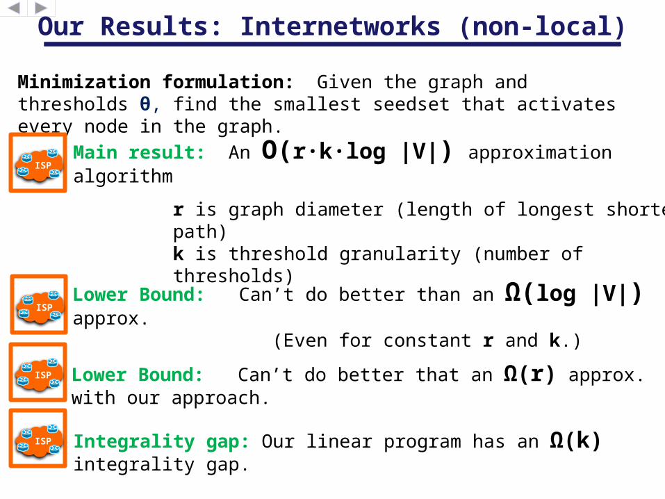
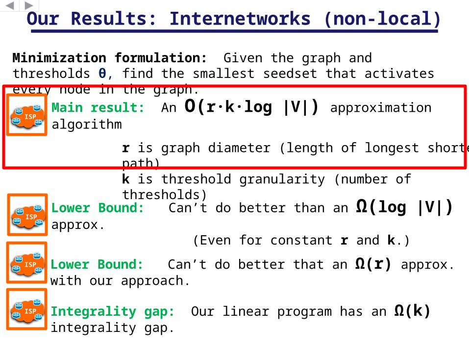
Minimization formulation: Given the graph and thresholds θ, find the smallest seedset that activates every node in the graph.
ISPMain result: An O(r∙k∙log |V|) approximation algorithm
r is graph diameter (length of longest shortest path)k is threshold granularity (number of thresholds)
Lower Bound: Can’t do better than an Ω(log |V|) approx. (Even for constant r and k.)
ISP
Lower Bound: Can’t do better that an Ω(r) approx. with our approach.
ISP
Integrality gap: Our linear program has an Ω(k) integrality gap. ISP
Our Results: Internetworks (non-local)
Minimization formulation: Given the graph and thresholds θ, find the smallest seedset that activates every node in the graph.
ISPMain result: An O(r∙k∙log |V|) approximation algorithm
r is graph diameter (length of longest shortest path)k is threshold granularity (number of thresholds)
Lower Bound: Can’t do better than an Ω(log |V|) approx. (Even for constant r and k.)
ISP
Lower Bound: Can’t do better that an Ω(r) approx. with our approach.
ISP
Integrality gap: Our linear program has an Ω(k) integrality gap.
ISP
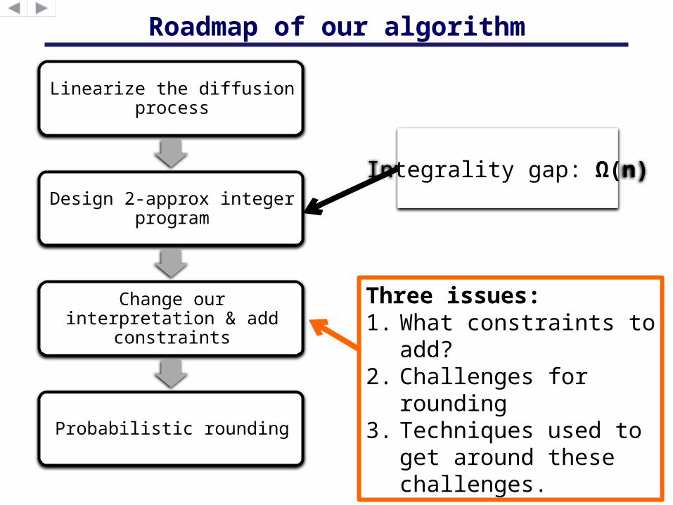
Roadmap of our algorithm
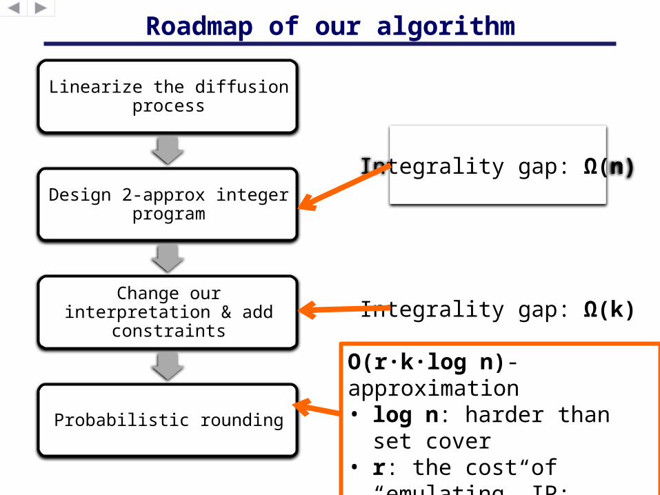
Linearize the diffusion process
Design 2-approx integer program
Change our interpretation & add constraints
Probabilistic rounding
Integrality gap: Ω(n)
Integrality gap: Ω(k)
O(r∙k∙log n)-approximation• log n: harder than set
cover• r: the cost of
“emulating” IP: requires a connected seedset
Linearization: terminology
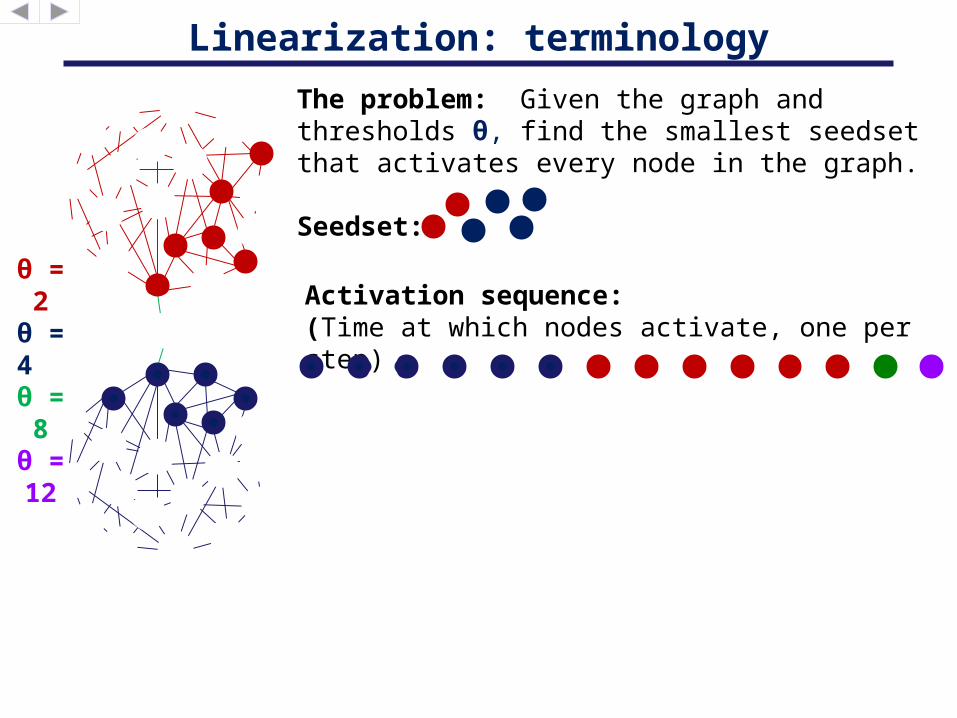
Seedset:
Activation sequence:(Time at which nodes activate, one per step)
The problem: Given the graph and thresholds θ, find the smallest seedset that activates every node in the graph.
θ = 2
θ = 4 θ = 8
θ = 12
Linearization: connectivity
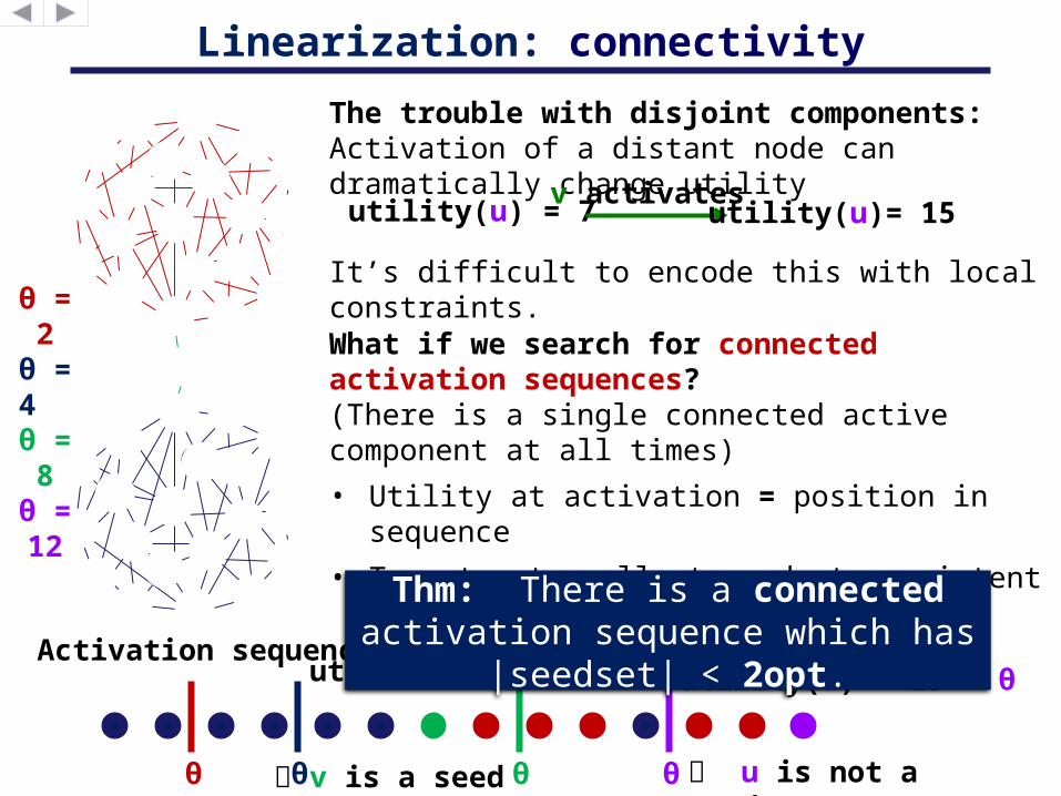
utility(u) = 7
The trouble with disjoint components: Activation of a distant node can dramatically change utility v activates
utility(u)= 15
It’s difficult to encode this with local constraints.
What if we search for connected activation sequences?(There is a single connected active component at all times)
• Utility at activation = position in sequence
• To extract smallest seedset consistent with sequence:
Just check if t > θ !Activation sequence
θ u is not a seed!
utility(u) = 15 > θ
θ = 2
θ = 4 θ = 8
θ = 12
θ θ θ
utility(v) < θ
v is a seed
Thm: There is a connected activation sequence which has |
seedset| < 2opt.
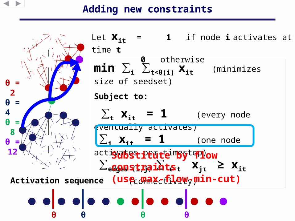
Activation sequence
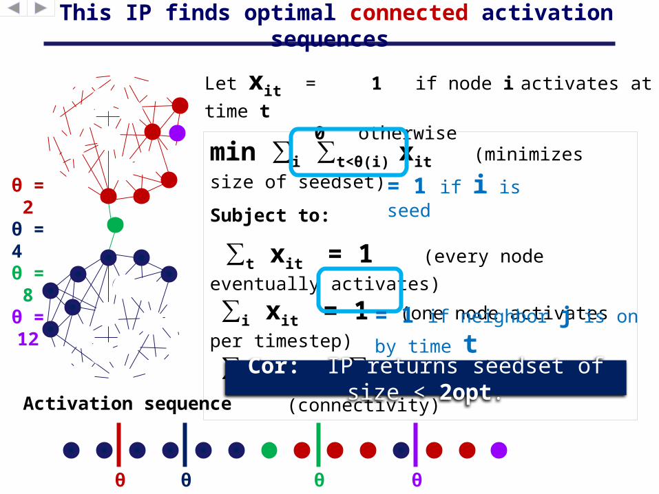
This IP finds optimal connected activation sequences
Let xit = 1 if node i activates at time t
0 otherwise
min ∑i ∑t<θ(i) xit (minimizes size
of seedset)
Subject to:
∑t xit = 1 (every node eventually
activates)
∑i xit = 1 (one node activates per
timestep)
∑edges (i,j) ∑ τ<t xjτ ≥ xit (connectivity)
Cor: IP returns seedset of size < 2opt.
θθ θ θ
θ = 2
θ = 4 θ = 8
θ = 12
= 1 if i is seed
= 1 if neighbor j is on by
time t
Roadmap of our algorithm
Linearize the diffusion process
Design 2-approx integer program
Change our interpretation & add constraints
Probabilistic rounding
Integrality gap: Ω(n)
Three issues:1. What constraints to
add?2. Challenges for
rounding3. Techniques used to
get around these challenges.
Activation sequence
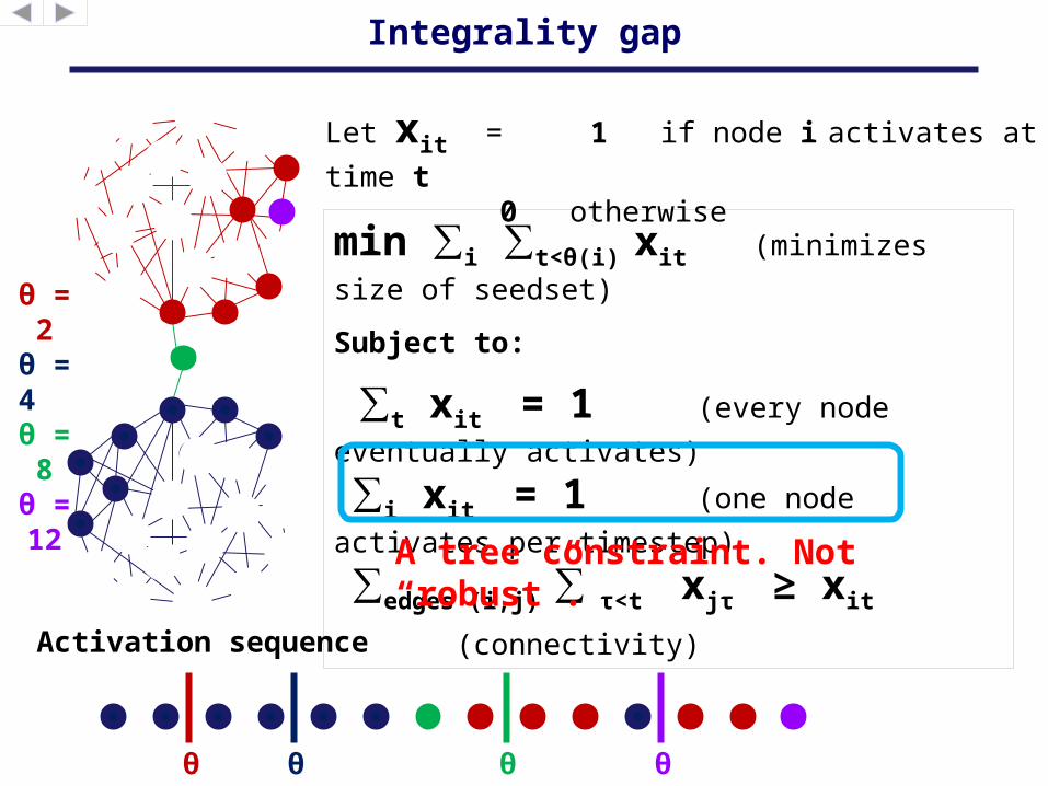
Integrality gap
Let xit = 1 if node i activates at time t
0 otherwise
min ∑i ∑t<θ(i) xit (minimizes size
of seedset)
Subject to:
∑t xit = 1 (every node
eventually activates)
∑i xit = 1 (one node activates
per timestep)
∑edges (i,j) ∑ τ<t xjτ ≥ xit (connectivity)
θθ θ θ
θ = 2
θ = 4 θ = 8
θ = 12 A tree constraint. Not
“robust”.
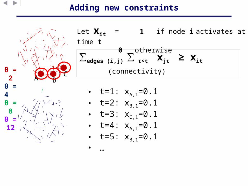
Adding new constraints
Let xit = 1 if node i activates at time t
0 otherwise
∑edges (i,j) ∑ τ<t xjτ ≥ xit (connectivity)θ =
2θ = 4 θ = 8
θ = 12
A BC
• t=1: xA,1=0.1
• t=2: xB,1=0.1
• t=3: xC,1=0.1
• t=4: xA,1=0.1
• t=5: xB,1=0.1• …
Activation sequence
Adding new constraints
Let xit = 1 if node i activates at time t
0 otherwise
min ∑i ∑t<θ(i) xit (minimizes size
of seedset)
Subject to:
∑t xit = 1 (every node
eventually activates)
∑i xit = 1 (one node activates
per timestep)
∑edges (i,j) ∑ τ<t xjτ ≥ xit (connectivity)
θθ θ θ
θ = 2
θ = 4 θ = 8
θ = 12 Substitute by flow
constraints(use max-flow-min-cut)
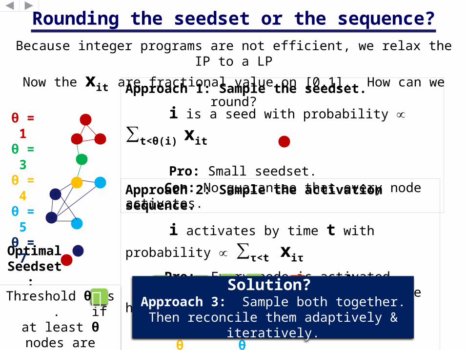
Rounding the seedset or the sequence?
Optimal Seedset
:
θ = 1
θ = 3
θ = 4
θ = 5
θ = 7
Because integer programs are not efficient, we relax the IP to a LP
Now the xit are fractional value on [0,1]. How can we round?
Approach 1: Sample the seedset.
i is a seed with probability ∝∑t<θ(i) xit
Pro: Small seedset. Con: No guarantee that every node activates.Approach 2: Sample the activation sequence.
i activates by time t with probability ∝
∑τ<t xiτ
Pro: Every node is activated. Con: Corresponding seedset can be huge!
Necessary
seedset:
θ θ θ θ θ
Threshold θ is . if at least θ
nodes are active by time θ
Solution?
Approach 3: Sample both together.Then reconcile them adaptively &
iteratively.
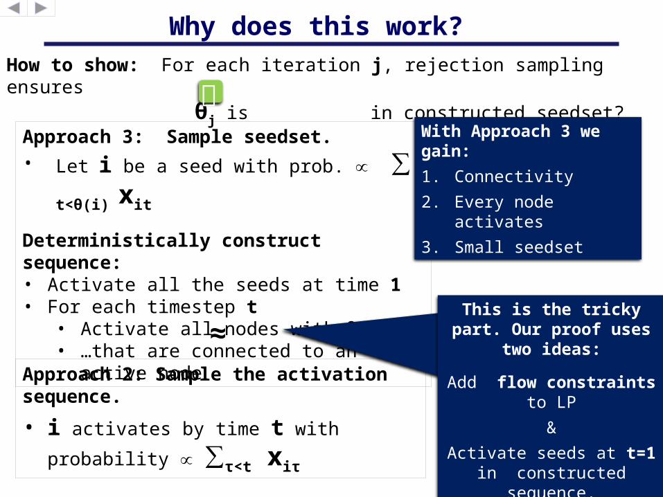
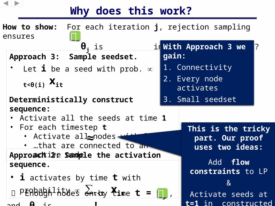
Why does this work? How to show: For each iteration j, rejection sampling ensures
θj is in constructed seedset?Approach 3: Sample seedset.
• Let i be a seed with prob. ∝ ∑ t<θ(i)
xit
Deterministically construct sequence:• Activate all the seeds at time 1• For each timestep t
• Activate all nodes with θ > t• …that are connected to an active
node≈
Approach 2: Sample the activation sequence.
• i activates by time t with probability ∝
∑τ<t xiτ
This is the tricky part. Our proof uses two
ideas:
Add flow constraints to LP
&
Activate seeds at t=1 in constructed sequence.
( connected seedset)
With Approach 3 we gain:
1. Connectivity
2. Every node activates
3. Small seedset
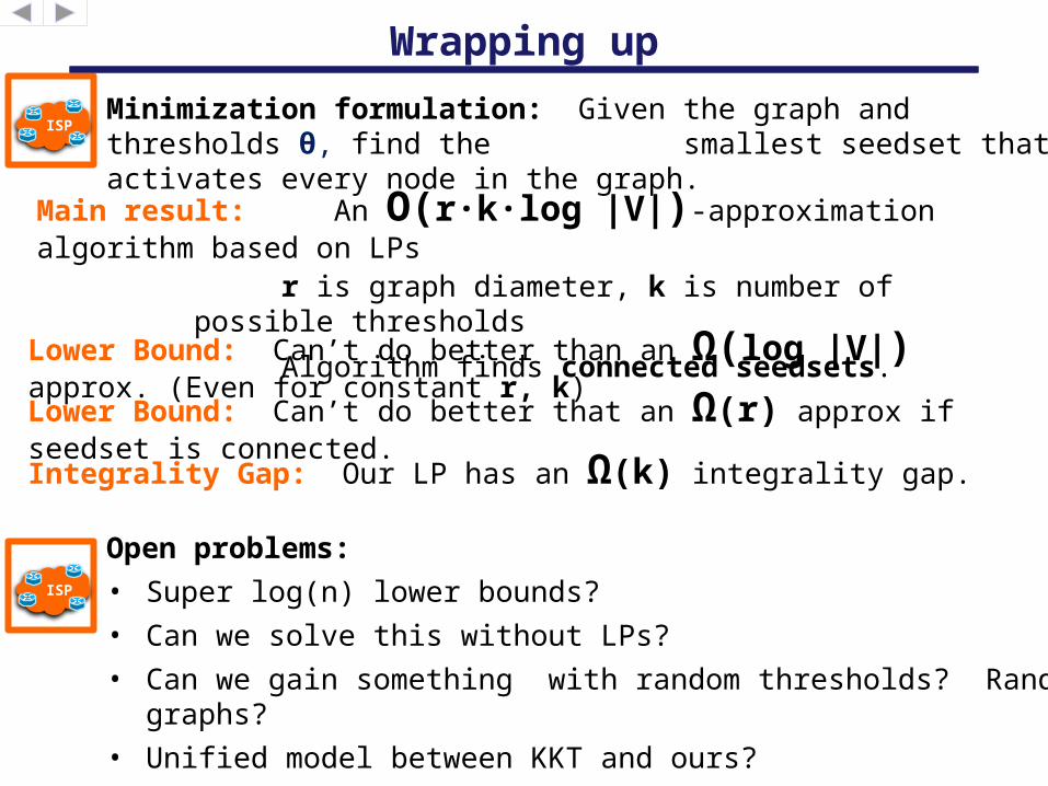
Wrapping up
Minimization formulation: Given the graph and thresholds θ, find the smallest seedset that activates every node in the graph.
ISP
Main result: An O(r∙k∙log |V|)-approximation algorithm based on LPs
r is graph diameter, k is number of possible thresholds
Algorithm finds connected seedsets. Lower Bound: Can’t do better than an Ω(log |V|) approx. (Even for constant r, k)Lower Bound: Can’t do better that an Ω(r) approx if seedset is connected.
Open problems:• Super log(n) lower bounds?• Can we solve this without LPs?• Can we gain something with random thresholds? Random
graphs?• Unified model between KKT and ours?
ISP
Integrality Gap: Our LP has an Ω(k) integrality gap.
Princeton University
Thanks!
Full report:
http://arxiv.org/abs/1202.2928
ISP
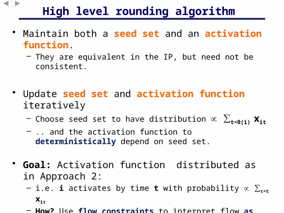
High level rounding algorithm
• Maintain both a seed set and an activation function. – They are equivalent in the IP, but need not be consistent.
• Update seed set and activation function iteratively– Choose seed set to have distribution ∝ ∑t<θ(i) xit
– .. and the activation function to deterministically depend on seed set.
• Goal: Activation function distributed as in
Approach 2:– i.e. i activates by time t with probability ∝ ∑τ<t xiτ
– How? Use flow constraints to interpret flow as probability mass.
– Performance degrade:• Emulate the IP process seed set connected a loss of r
in approx. ratio.
Seedset:
Optimal (disconnected) activation sequence
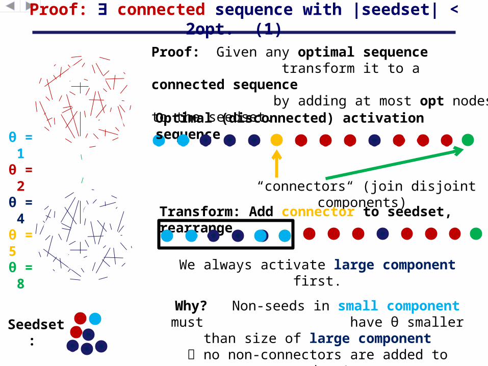
Proof: ∃ connected sequence with |seedset| < 2opt. (1)
Proof: Given any optimal sequence transform it to a connected sequence by adding at most opt nodes to the seedset.
“connectors“ (join disjoint components)
Transform: Add connector to seedset, rearrange
We always activate large component first.
Why? Non-seeds in small component must have θ smaller than size of
large component no non-connectors are added to seedset!
θ = 1
θ = 2
θ = 4
θ = 5 θ = 8
Optimal (disconnected) activation sequence
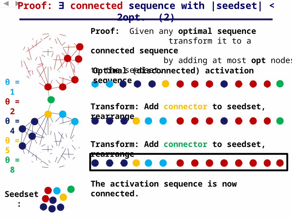
Proof: ∃ connected sequence with |seedset| < 2opt. (2)
Transform: Add connector to seedset, rearrange
Transform: Add connector to seedset, rearrange
Seedset:
The activation sequence is now connected.
Proof: Given any optimal sequence transform it to a connected sequence by adding at most opt nodes to the seedset.
θ = 1
θ = 2
θ = 4
θ = 5 θ = 8
Optimal (disconnected) activation sequence
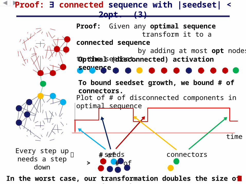
Proof: ∃ connected sequence with |seedset| < 2opt. (3)
To bound seedset growth, we bound # of connectors.
seeds
time
Plot of # of disconnected components in optimal sequence
connectors # of > # of
In the worst case, our transformation doubles the size of the seedset!
Every step up needs a step
down
Proof: Given any optimal sequence transform it to a connected sequence by adding at most opt nodes to the seedset.

Princeton University
Part II: How do we round this?
Iterative and adaptive rounding with both the seedset and
sequence.
We return connected seedsets instead of connected activation
sequences. ( O(r)-approx instead of 2-approx )
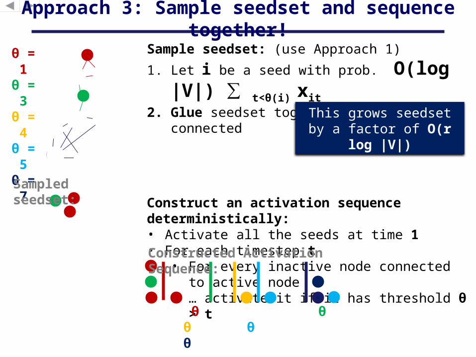
Sample seedset: (use Approach 1)
1. Let i be a seed with prob. O(log |V|) ∑ t<θ(i) xit
2. Glue seedset together so it’s connected
Construct an activation sequence deterministically:• Activate all the seeds at time 1• For each timestep t
• For every inactive node connected to active node
• … activate it if it has threshold θ > t
Approach 3: Sample seedset and sequence together!
θ = 1
θ = 3
θ = 4
θ = 5
θ = 7
θ θ θ θ θ
Constructed Activation Sequence:
Sampled seedset:
This grows seedset by a factor of O(r log |V|)
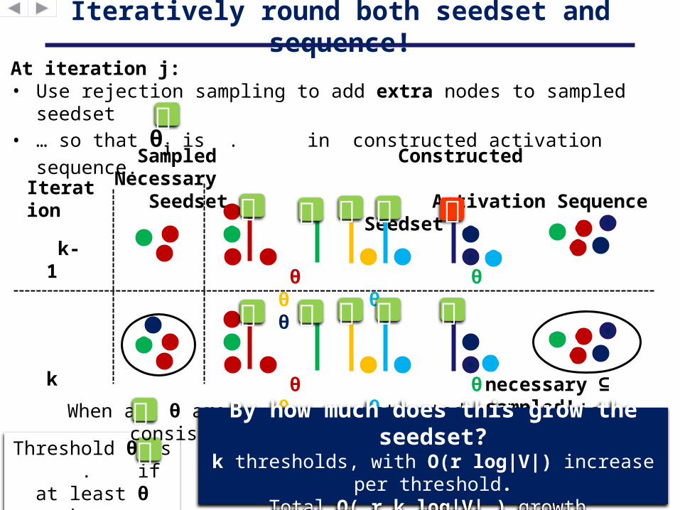
Iteratively round both seedset and sequence!
Sampled Constructed Necessary Seedset Activation Sequence Seedset
At iteration j:• Use rejection sampling to add extra nodes to sampled seedset• … so that θj is . in constructed activation sequence.
Iteration
k-1
necessary ⊆sampled!
θ θ θ θ θ
k
θ θ θ θ θ
Threshold θ is . if at least θ
nodes are active by time θ
When all θ are , , constructed sequence is consistent with the sampled seedset.
By how much does this grow the seedset?
k thresholds, with O(r log|V|) increase per threshold.
Total O( r k log|V| ) growth.
Why does this work? How to show: For each iteration j, rejection sampling ensures
θj is in constructed seedset?Approach 3: Sample seedset.
• Let i be a seed with prob. ∝ ∑ t<θ(i)
xit
Deterministically construct sequence:• Activate all the seeds at time 1• For each timestep t
• Activate all nodes with θ > t• …that are connected to an active
node≈
Approach 2: Sample the activation sequence.
• i activates by time t with probability ∝
∑τ<t xiτ Enough nodes on by time t = θj , and
θj is !
This is the tricky part. Our proof uses
two ideas:
Add flow constraints to LP
&
Activate seeds at t=1 in constructed
sequence.
( connected seedset)
With Approach 3 we gain:
1. Connectivity
2. Every node activates
3. Small seedset
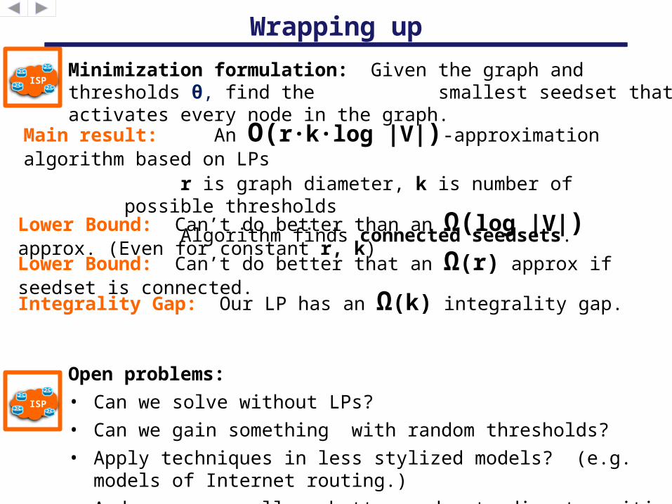
Wrapping up
Minimization formulation: Given the graph and thresholds θ, find the smallest seedset that activates every node in the graph.
ISP
Main result: An O(r∙k∙log |V|)-approximation algorithm based on LPs
r is graph diameter, k is number of possible thresholds
Algorithm finds connected seedsets. Lower Bound: Can’t do better than an Ω(log |V|) approx. (Even for constant r, k)Lower Bound: Can’t do better that an Ω(r) approx if seedset is connected.
Open problems:• Can we solve without LPs?• Can we gain something with random thresholds?• Apply techniques in less stylized models? (e.g. models of
Internet routing.)• And more generally – better understanding transitions to new
technology
ISP
Integrality Gap: Our LP has an Ω(k) integrality gap.

Princeton University
Thanks!
To appear at SODA’13
http://arxiv.org/abs/1202.2928
ISP

Standard submodularity tricks fail in our setting!
E[on | clique and v ] ≈ n + Pr[1st blue on] E[clique on] ≈ n + 1/2 ∙ n/2
E[on | clique] ≈ n + Pr[v on] Pr[1st blue on] ] E[clique on ] ≈ n + 1/2 ∙ 1/2 ∙ n/2
E[on | v] ≈ 3
Submodularity:
E[on | clique and v ] ≤ E[on | clique ] + E[on| v]n + n/4 n + n/8 3>
Not submodular!
Let’s use the standard trick of choosing thresholds uniformly at
random.
0 0.3 0 0 0 0.6 0 0.1
0 0 0.3 0 0.6 0.1 0 0
0 0 0 0.3 0 0 0 0.7
t
i
θ θ θ
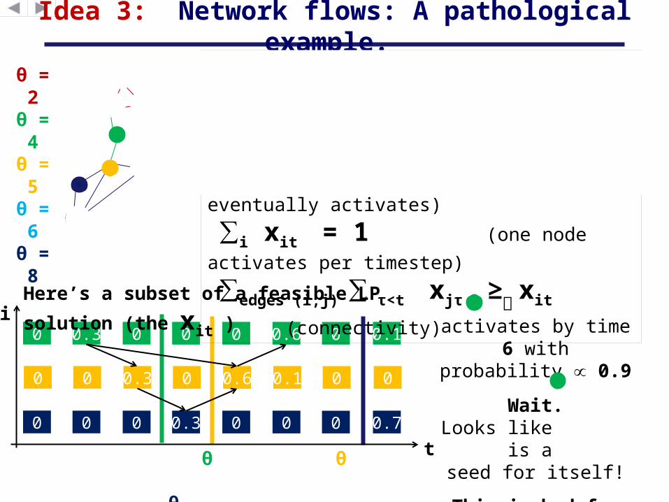
Idea 3: Network flows: A pathological example.
min ∑i ∑t<θ(i) xit (minimizes size
of seedset)
Subject to:
∑t xit = 1 (every node
eventually activates)
∑i xit = 1 (one node
activates per timestep)
∑edges (i,j) ∑ τ<t xjτ ≥ xit (connectivity)
θ = 2
θ = 4
θ = 5
θ = 6
θ = 8Here’s a subset of a feasible LP
solution (the xit ) activates by
time 6 with probability ∝ 0.9
Wait.Looks like is a
seed for itself!
This is bad for us.

0 0.3 0.1 0 0 0.6 0 0
0 0 0.3 0 0.6 0.1 0 0
0 0 0 0.3 0 0 0 0.7
t
i
θ θ θ
0 0.3 0.1 0 0 0.6 0 0
0 0 0.3 0 0.6 0.1 0 0
0 0 0 0.3 0 0 0 0.7
t
i
θ θ θ
Idea 3: Network flows: Adding flow constraints
θ = 2
θ = 4
θ = 5
θ = 6
θ = 81 0 0 0 0 0 0 0
source
The ( , 2) flow problem
sinks
We add a few extra constraints to the LP1) Constrain a source node to start at time
12) Require a solution to each (i,t) flow
problem.
The source must supply the
demand of all the sinks over paths of capacity given by
node and edge weights.
1
0.6
This flow problem has no solution, since we can’t supply the
sink!
No morepathological example!
Q. How does this achieve:
“ i activates by time t with prob. ∝∑τ<t xiτ”
A. The flow constraints ensure that i has a path to at least one active seed with this
probability!
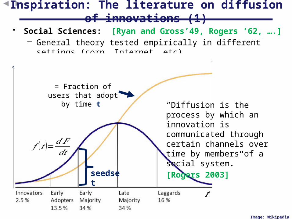
Inspiration: The literature on diffusion of innovations (1)
• Social Sciences: [Ryan and Gross’49, Rogers ’62, ….]– General theory tested empirically in different settings (corn,
Internet, etc)
Image: Wikipedia
𝑡
= Fraction of users that adopt by time t
𝑓 (𝑡 )=𝑑𝐹𝑑𝑡
“Diffusion is the process by which an innovation is communicated through certain channels over time by members of a social system.”[Rogers 2003]
seedset
• Social Sciences: [Ryan and Gross’49, Rogers ’62, ….]– General theory tested empirically in different settings (corn,
Internet, etc)
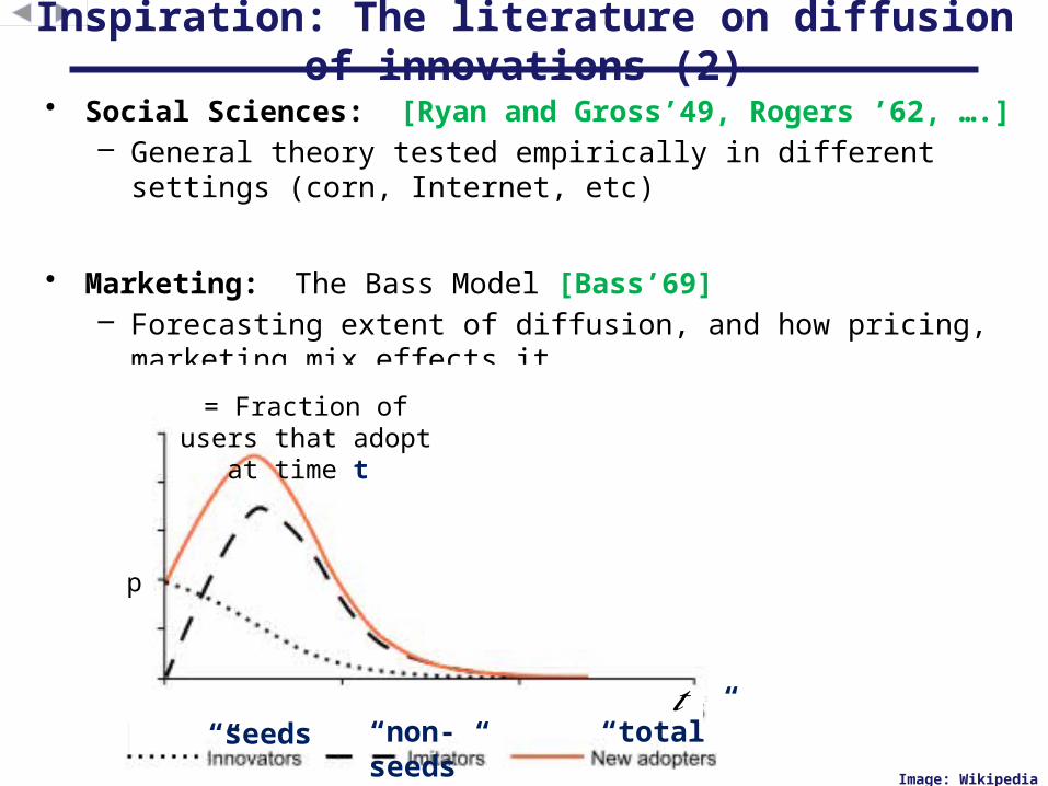
• Marketing: The Bass Model [Bass’69]– Forecasting extent of diffusion, and how pricing, marketing
mix effects it
Inspiration: The literature on diffusion of innovations (2)
p
𝑡
Image: Wikipedia
= Fraction of users that adopt at time t
“seeds”
“non-seeds”
“total”
• Social Sciences: [Ryan and Gross’49, Rogers ’62, ….]– General theory tested empirically in different settings (corn,
Internet, etc)
• Marketing: The Bass Model [Bass’69]– Forecasting extent of diffusion, and how pricing, marketing
mix effects it
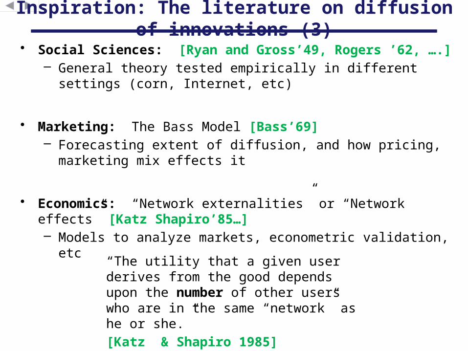
• Economics: “Network externalities” or “Network effects” [Katz Shapiro’85…] – Models to analyze markets, econometric validation, etc
Inspiration: The literature on diffusion of innovations (3)
“The utility that a given user derives from the good depends upon the number of other users who are in the same “network” as he or she.”[Katz & Shapiro 1985]
• Social Sciences: [Ryan and Gross’49, Rogers ’62, ….]– General theory tested empirically in different settings (corn,
Internet, etc)
• Marketing: The Bass Model [Bass’69]– Forecasting extent of diffusion, and how pricing, marketing
mix effects it
• Economics: “Network externalities” or “Network effects” [Katz Shapiro’85…] – Models to analyze markets, econometric validation, etc
• Popular Science: “Metcalfe’s Law” [Metcalfe 1995]
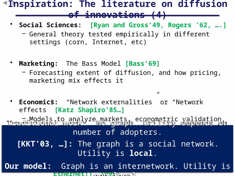
Inspiration: The literature on diffusion of innovations (4)
“The utility that a single user gets for being part of a network of n users scales as n.”[Metcalfe, (inventor of Ethernet!), 1995]
Traditional work: No graph. Utility depends on number of adopters.
[KKT’03, …]: The graph is a social network. Utility is local.
Our model: Graph is an internetwork. Utility is non-local.
Princeton University
Part I: From global to local.
(via a 2-approximation )