The Complex Zeros of Random Polynomials. - Princeton University

THE COMPLEX ZEROS OF RANDOM POLYNOMIALS

LARRY A. SHEPP AND ROBERT J. VANDERBEI

ABSTRACT. Mark Kac gave an explicit formula for the expectation of the number, νn(Ω), of zerosof a random polynomial,

Pn(z) =

n−1∑j=0

ηjzj ,

in any measurable subset Ω of the reals. Here, η0, . . . , ηn−1 are independent standard normal ran-dom variables. In fact, for each n > 1, he obtained an explicit intensity function gn for which

Eνn(Ω) =

∫Ω

gn(x)dx.

Here, we extend this formula to obtain an explicit formula for the expected number of zeros in anymeasurable subset Ω of the complex plane IC. Namely, we show that

Eνn(Ω) =

∫Ω

hn(x, y)dxdy +

∫Ω∩IR

gn(x)dx,

where hn is an explicit intensity function. We also study the asymptotics of hn showing that forlarge n its mass lies close to, and is uniformly distributed around, the unit circle.

1. INTRODUCTION.

More than fifty years ago, Mark Kac [7] gave an explicit formula for the expectation of thenumber, νn(Ω), of zeros of a random polynomial,

(1.1) Pn(z) =n−1∑j=0

ηjzj, z ∈ IC,

in any measurable subset Ω of the reals. Here, η0, . . . , ηn−1 are independent standard normalrandom variables (which Kac argues is the most natural choice for a “typical” polynomial sincethis distribution is invariant under orthogonal transformations - but of course other choices for themeasure are also interesting). In fact, for each n > 1, he obtained an explicit intensity function gnfor which

Eνn(Ω) =

∫Ω

gn(x)dx.

1991 Mathematics Subject Classification. Primary 30C15, Secondary 30B20, 26C10, 60B99.Second author’s research supported by AFOSR through grant AFOSR-91-0359.

1

2 LARRY A. SHEPP AND ROBERT J. VANDERBEI

Here, we extend this result by deriving an explicit formula for the expected number of zeros in anymeasurable subset Ω of the complex plane IC. Namely, we show that

Eνn(Ω) =

∫Ω

hn(x, y)dxdy +

∫Ω∩IR

gn(x)dx,

where hn is an explicit intensity function. (Note that we make the usual identification between apoint z of the complex plane and its real and imaginary parts, x and y.)

The intensity function hn is conveniently expressed in terms of the following three real-valuedfunctions defined on IC

Bk(z) =n−1∑j=0

jk|z|2j, z ∈ IC, k = 0, 1, 2,

and the following two complex-valued functions

Ak(z) =n−1∑j=0

jkz2j, z ∈ IC, k = 0, 1.

Finally, let

(1.2) D0(z) =√B2

0(z)− |A0|2(z).

Our main result is

Theorem 1.1. For each region Ω ∈ IC,

(1.3) Eνn(Ω) =

∫Ω

hn(x, y)dxdy +

∫Ω∩IR

gn(x)dx,

where

hn =B2D

20 −B0(B2

1 + |A1|2) +B1(A0A1 + A0A1)

π|z|2D30

,

and

gn =(B0B2 −B2

1)1/2

π|z|B0

.

As already mentioned, Kac [7] was the first to study the real zeros for random polynomials ofthis type and he obtained the intensity function gn. Somewhat earlier (but delayed in publicationby the war), Rice [12] obtained a similar formula for the expected number of zeros of a generalstochastic process X(t) again depending on a real parameter t but did not consider the special casewhen X is a polynomial in t. Here, we obtain Kac’s gn as a consequence of our analysis of thezeros in the complex plane.

ZEROS OF RANDOM POLYNOMIALS 3

While the definition of hn in Theorem 1.1 looks rather complicated, it is nevertheless amenableboth to computation (see Figures 1 to 6) and to asymptotic analysis. Indeed, the computed plotsappearing on the left-hand side in Figures 1 to 6 clearly show that as n gets large the zeros tend tolie very close to the unit circle and, ignoring the real roots, appear to be approximately uniformlydistributed around the circle. Regarding analysis, the next Theorem shows that the intensities hnand gn have well-defined limits as n tends to infinity. These limits are best expressed in terms ofthe following functions:

(1.4) B(z) =1

1− |z|2,

(1.5) A(z) =1

1− z2,

and

(1.6) D(z) =√B2(z)− |A|2(z).

Theorem 1.2. We have the following limits:

h = limnhn =

|B|Dπ

and

g = limngn =

1

π|B|.

The limit functions, h and g, can be viewed as intensity functions for the zeros of the randompower series

P (z) =∞∑j=0

ηjzj

(at least within its radius of convergence, |z| < 1).

Following the initial work of Kac and Rice, a large body of research on zeros of random polyno-mials has appeared – see [2] for a fairly complete account including an extensive list of references.Most of this work has focused on the real zeros; [4], [5] and [14] being a few notable exceptions.Also, the recent paper of Edelman and Kostlan [3] gives a very elegent geometric treatment of theproblem.

In the following section, we derive explicit formulas for the intensity functions hn and gn. Thenin Section 3, we study the limiting form of these functions as n tends to infinity. Section 4 presentsmore delicate asymptotic analysis that shows how hn and gn behave when n is large, but finite.Next, in Section 5, we discuss computational issues and finally, in Section 6 we offer some specu-lation and suggest future research directions.


We end this section by remarking that even though we usually consider the entire complex plane,it suffices in general to study simply the unit disk centered at the origin since, given a randompolynomial Pn(z), the transformation to znPn(1/z) produces a new random polynomial whosezeros are exactly the reciprocals of the zeros of Pn(z). Hence, for any set A, we have that

(1.7) Eνn(A−1) = Eνn(A),

where A−1 = z : z−1 ∈ A. From this it follows easily that any intensity function, say h mustsatisfy

(1.8) h(z) = h(1/z)1

|z|2.

2. THE INTENSITY FUNCTIONS hn AND gn.

This section is devoted to the proof of Theorem 1.1. We begin with

Proposition 2.1. For each region Ω ∈ IC whose boundary intersects the real axis at most onlyfinitely many times,

(2.1) Eνn(Ω) =1

2πi

∫∂Ω

1

zF (z)dz,

where

(2.2) F =B1D0 +B0B1 − A0A1

B0D0 +B20 − A0A0

.

Proof. The argument principle (see, e.g., [1], p. 151) gives an explicit formula for the randomvariable νn(Ω), namely

(2.3) νn(Ω) =1

2πi

∫∂Ω

P ′n(z)

Pn(z)dz.

Taking expectations in (2.3) and then interchanging expectation and contour integration (thejustification of which is tedious but doable), we get

(2.4) Eνn(Ω) =1

2πi

∫∂Ω

EP ′n(z)

Pn(z)dz.

To facilitate computations, it is advantagous to multiply and divide by z (multiplying inside theexpectation and dividing outside). The following Lemma shows that away from the real axis thefunction

(2.5) F (z) = EzP ′n(z)

Pn(z)


simplifies to the expression given in (2.2) and, since we’ve assumed that ∂Ω intersects the real axisat only finitely many points, this finishes the proof.

Lemma 2.2. Let F denote the function defined by (2.5). Off the real axis,

F =B1D0 +B0B1 − A0A1

B0D0 +B20 − A0A0

.

On the real axis, F has a jump discontinuity. Indeed, for each x ∈ IR,

limz→x: Im(z)>0

F =B1 − i(B0B2 −B2

1)1/2

B0

and

limz→x: Im(z)<0

F =B1 + i(B0B2 −B2

1)1/2

B0

.

Proof. First we consider the case where z does not lie on the real axis. Note that Pn(z) and zP ′n(z)are complex Gaussian random variables. It is convenient to work with their real and imaginaryparts,

Pn(z) = ξ1 + iξ2,(2.6)zP ′n(z) = ξ3 + iξ4,(2.7)

which are just linear combinations of the original standard normal random variables:

ξ1 =∑n−1

j=0 ajηj, ξ2 =∑n−1

j=0 bjηj,

ξ3 =∑n−1

j=0 cjηj, ξ4 =∑n−1

j=0 djηj.

The coefficients in these linear combinations are given by

(2.8)

aj = Re(zj) =zj + zj

2,

bj = Im(zj) =zj − zj

2i,

cj = jaj,dj = jbj.

Put ξ = [ ξ1 ξ2 ξ3 ξ4 ]T . The covariance among these four Gaussian random variables is easyto compute:

(2.9) Cov(ξ) = EξξT =

aTa aT b aT c aTdbTa bT b bT c bTdcTa cT b cT c cTddTa dT b dT c dTd

We now represent these four correlated Gaussian random variables in terms of four standard nor-mals. To this end, we seek a lower triangular matrix L = [ lij ] such that the vector ξ is equal indistribution to Lζ , where ζ = [ ζ1 ζ2 ζ3 ζ4 ]T is a vector of four independent standard normal


random variables. The following simple calculation shows that L is the Cholesky factor for thecovariance matrix:

(2.10) Cov(ξ) = EξξT = ELζζTLT = LLT .

Now, since ξ D= Lζ and L is lower triangular (the symbol D

= denotes equality in distribution), weget that

zP ′n(z)

Pn(z)=

ξ3 + iξ4

ξ1 + iξ2

D=

(l31 + il41)ζ1 + (l32 + il42)ζ2 + (l33 + il43)ζ3 + il44ζ4

(l11 + il21)ζ1 + il22ζ2

.

Hence, exploiting the independence of the ζi’s, we see that

(2.11) F (z) = EzP ′n(z)

Pn(z)= E

αζ1 + βζ2

γζ1 + δζ2

,

whereα = l31 + il41 β = l32 + il42

γ = l11 + il21 δ = il22.

Splitting up the numerator in (2.11) and exploiting the exchangeability of ζ1 and ζ2, we can rewritethe expectation as follows:

F (z) =α

δf(γ/δ) +

β

γf(δ/γ),

where f is a complex-valued function defined on IC \ IR by

f(w) = Eζ1

wζ1 + ζ2

.

The expectation appearing in the definition of f can be explicitly computed. Indeed,

f(w) =1

2π

∫ 2π

0

∫ ∞0

ρ cos θ

wρ cos θ + ρ sin θe−ρ

2/2ρdρdθ

=1

2π

∫ 2π

0

dθ

w + tan θ

and the substitution u = tan θ can then be used to rewrite this integral as

f(w) =1

π

∫ ∞−∞

1

(w + u)(1 + u2)du

which is easily solved using the calculus of residues. The final result is that

f(w) =

1

w + i, Im(w) > 0,

1

w − i, Im(w) < 0.


Recalling the definition of δ and γ, we see that

γ

δ=l21

l22

− i l11

l22

.

In general, l11 and l22 are just nonnegative. However, it is not hard to show that they are bothstrictly positive whenever z has a nonzero imaginary part. Hence, γ/δ lies in the lower half-plane,δ/γ lies in the upper half-plane, and

F (z) =α

δ

1γδ− i

+β

γ

1δγ

+ i

=iα + β

iγ + δ

=l32 − l41 + i(l31 + l42)

−l21 + i(l11 + l22).(2.12)

At this point, we need explicit formulas for the elements of the Cholesky factor L. From (2.9) and(2.10), we see that

aTa = l211

bTa = l21l11

cTa = l31l11

dTa = l41l11

bT b = l221 + l222

cT b = l31l21 + l32l22

dT b = l41l21 + l42l22.


Solving these equations in succession, we get

l11 =aTa√aTa

l21 =bTa√aTa

l31 =cTa√aTa

l41 =dTa√aTa

l22 =(aTa)(bT b)− (bTa)2

√aTaR

l32 =(aTa)(cT b)− (cTa)(bTa)√

aTaR

l42 =(aTa)(dT b)− (dTa)(bTa)√

aTaR,

whereR =

√(aTa)(bT b)− (bTa)2.

Substituting these expressions into (2.12) and simplifying, we see that

(2.13) F (z) =−dTa+ icTa− i

(aTa(−dT b+ icT b)− (−dTa+ icTa)bTa

)/R

−bTa+ iaTa+ iR.

Recalling the definitions of aj , bj , cj , and dj given in (2.8), it is easy to check that the followingidentities hold:

aTa = +1

4(A0 + 2B0 + A0),

bTa = − i4

(A0 − A0),

cTa = +1

4(A1 + 2B1 + A1),

dTa = − i4

(A1 − A1),

bT b = −1

4(A0 − 2B0 + A0),

cT b = − i4

(A1 − A1),

dT b = −1

4(A1 − 2B1 + A1).


Plugging these expressions into (2.13) and simplifying, we get that

(2.14) F (z) =A1 +B1 + (A0B1 +B0B1 − A1B0 − A0A1)/D0

A0 +B0 +D0

,

where D0 is given in (1.2). It turns out that further simplification occurs if we make the denomi-nator real by the usual technique of multiplying and dividing by its complex conjugate. We leaveout the algebraic details except to mention that a factor of A0 + 2B0 + A0 cancels out from thenumerator and denominator leaving us with

(2.15) F (z) =B1D0 +B0B1 − A0A1

D0(B0 +D0),

or, expanding out D20,

(2.16) F (z) =B1D0 +B0B1 − A0A1

B0D0 +B20 − A0A0

.

The expression in (2.15) is as simple as possible, whereas (2.16) illustrates a certain parallelismbetween the numerator and denominator.

Now consider a point x on the real axis. On the reals, Ak = Bk, k = 0, 1, and so D0 = 0.Hence, the right-hand side in (2.15) is an indeterminate form. To analyze the limiting behavior ofF near the real axis, we first divide the numerator and denominator by D0:

(2.17) F =B1 +

B0B1 − A0A1

D0

B0 +D0

.

Now, only the ratio in the numerator is indeterminate. To study it, we write z = reiθ and investigatethe numerator and denominator of this ratio when θ is small. From the definitions, we see that

B0B1 − A0A1 =∑j,k

kr2(k+j)(1− e2(k−j)θi)(2.18)

=∑j,k

kr2(k+j)2(j − k)θi+ o(θ)

= 2θi(B21 −B0B2) + o(θ)

and

B20 − |A0|2 =

∑j,k

r2(k+j)(1− e2(k−j)θi)(2.19)

= −∑j,k

r2(k+j)2(k − j)2θ2i2 + o(θ2)

= 4θ2(B0B2 −B21) + o(θ2).


Hence, recalling that D0 =√B2

0 − |A0|2, we see that

B0B1 − A0A1

D0

= sgn(θ)iB2

1 −B0B2 + o(θ)

(B0B2 −B21 + o(θ2))1/2

= −sgn(θ)i(B0B2 −B21)1/2 + o(θ).(2.20)

Combining (2.17) and (2.20), we get the desired limits expressing the jump discontinuity on thereal axis.

Proof of Theorem 1.1. Without loss of generality, it suffices to consider regions Ω that are eitherregions that do not intersect the real axis or polar rectangles that do intersect the real axis. Webegin by considering a region Ω that does not intersect the real axis. Applying Stokes’ theorem tothe expression for Eνn(Ω) given in Proposition 2.1, we see that

Eνn(Ω) =1

π

∫Ω

1

z

∂

∂zF (z, z)dxdy.

Note that we are now writing F (z, z) to emphasize the fact that F depends on both z and z. Lettingthe dagger symbol stand for the derivative with respect to z, we see from Lemma 2.2 that

∂F

∂z=

(B0D0 +B2

0 − A0A0)(B†1D0 +B1D†0 +B†0 +B0B

†1 − A

†0A1)

−(B1D0 +B0B1 − A0A1)(B†0D0 +B0D†0 + 2B0B

†0 − A

†0A0)

/(B0D0 +B2

0 − |A0|2)2.

From their definitions, it is easy to verify that

B†0 =B1

z, A†0 =

2A1

z, B†1 =

B2

z.

Recalling that D0 =√B2

0 − |A|2, we get that

D†0 =B0B1 − A0A1

zD0

.

Substituting these formulas for the derivatives into the expression given above for ∂F/∂z and thenengaging in tedious algebraic simplifications (a computer algebra package such as Mathematicawould be useful here, but we confess that we did this by hand), we eventually arrive at the fact that(πz)−1∂F (z, z)/∂z equals the expression given in Theorem 1.1 for hn.

Now consider a polar rectangle that covers a portion of the real axis. In other words, let Ω bethe angular interval (−θ, θ) crossed with a radial interval (r0, r1) (we have assumed without lossof generality that the polar rectangle does not intersect the negative part of the real axis). Writing


down the contour integral for Eνn(Ω) given by Proposition 2.1 and letting θ tend to 0, we see that

Eνn((r0, r1)) =1

2πi

∫ r1

r0

F (r−)− F (r+)

rdr,

where νn((r0, r1)) denotes the number of zeros in the interval (r0, r1) of the real axis and

F (r−) = limz→r:Im(z)<0

F (z) and F (r+) = limz→r:Im(z)>0

F (z).

Hence, from Lemma 2.2, we see that

gn(r) =1

2πi

F (r−)− F (r+)

r=

√B0B2 −B2

1

πrB0

.

This completes the proof.

3. LIMITING INTENSITY.

In this section we study the limits obtained by letting n tend to infinity. As mentioned in theintroduction, these limits can be viewed as intensity functions for the limiting random power series.We begin by proving Theorem 1.2:

Proof of Theorem 1.2. The sums used to define the functions Bk and Ak can be summed explicitly.Recalling the functions A and B defined by (1.5) and (1.4), respectively, we have

B0 = B − |z|2nB,(3.1)B1 = |z|2B2 −

(n|z|2nB + |z|2n+2B2

),(3.2)

B2 = |z|2(1 + |z|2)B3

−(n2|z|2nB + 2n|z|2n+2B2 + |z|2n+2(1 + |z|2)B3

),(3.3)

A0 = A− z2nA,

A1 = z2A2 −(nz2nA+ z2n+2A2

).

For |z| < 1, we have the following limits:

limn→∞

B0 = B,(3.4)

limn→∞

B1 = |z|2B2,(3.5)

limn→∞

B2 = |z|2(1 + |z|2)B3,(3.6)

limn→∞

A0 = A,

limn→∞

A1 = z2A2.


Using these limits, it is easy to check that

limn→∞

(B2B

20 −B0B

21

)= |z|2B5,

and

limn→∞

(−B2|A0|2 −B0|A1|2 +B1(A0A1 + A0A1)

)= −|z|2B|A|2

(B2 + |zB − zA|2

).

Then, using the definitions of A, B, and D, we see that

|zB − zA|2 = D2.

Substituting these ingredients into the expression given in Theorem 1.1 for hn and simplifying, wefind that

limn→∞

hn =|z|2B5 − |z|2B|A|2 (B2 + |zB − zA|2)

π|z|2D3

=BD

π.(3.7)

The case |z| > 1 is more tedious (and less interesting!). We can either refer to the inversionsymmetry formula (1.8) or we can compute in a manner similar to the |z| < 1 case. Opting forthe detailed computation, we note that this time we must keep track of terms involving the threehighest orders: n2|z|2n, n|z|2n, and |z|2n. Then we compute the numerator of the right-hand factorin the expression given in Theorem 1.1 for hn and we discover that the two highest-order termscancel out leaving terms of the order |z|2n as the highest remaining order. Indeed,

B2B20 −B0B

21 = −|z|6n|z|2B5 + o(|z|6n),

−B2|A0|2 −B0|A1|2 +B1(A0A1 + A0A1) =

|z|6n|z|2B|A|2 (B2 + |zB − zA|2) + o(|z|6n),

andD2

0 = |z|4nD2 + o(|z|4n).

Hence, the numerator and denominator of the right-hand factor both have |z|6n as their highest or-der terms, so this factor can be canceled. For the left-hand factor, both numerator and denominatorhave |z|4n as their highest order terms. Eliminating these and passing to the limit, we get

(3.8) limn→∞

hn =−BDπ

.

Bearing in mind that B > 0 for |z| < 1 and B < 0 for |z| > 1, we see that (3.7) and (3.8) canbe combined to give the formula asserted for h.


The same method is used to find limn→∞ gn. Indeed, for |z| < 1, we use (3.4), (3.5), and (3.6)to see that

limn→∞

gn =1

πB.

For |z| > 1, we retain the three highest order terms from (3.1), (3.2), and (3.3). As before the twohighest order terms cancel out in the expression for B0B2 −B2

1 leaving us with

B0B2 −B21 = |z|4n|z|2B4 + o(|z|4n).

From this expression, we easily see that

limn→∞

gn = − 1

πB,

which completes the proof.

4. ASYMPTOTICS FOR THE NUMBER OF ROOTS.

In this section we derive limiting expressions for the expected number of zeros in disks andsectors. We start with the disk, B(r), of radius r centered at 0.

Theorem 4.1. For r < 1,

limn→∞

Eνn(B(r)) =r2

1− r2+O(1).

Proof. From Proposition 2.1, we have that

Eνn(B(r)) =1

2πi

∫∂B(r)

1

zF (z)dz

=1

2π

∫ 2π

0

F (z)dθ.

Now, applying the bounded convergence theorem, we see that

limn→∞

Eνn(B(r)) =1

2π

∫ 2π

0

limn→∞

F (z)dθ

and, using the expression given in (2.15) for F , we get that

limn→∞

F (z) =|z|2B2D +B|z|2B2 − Az2A2

(B +D)D.

Adding and subtracting |z|2B|A|2 from the numerator and using the fact that |z|2B = r2/(1− r2)on the contour of integration, we see that

(4.1) limn→∞

F (z) =r2

1− r2+

|A|2

(B +D)D

(|z|2B − z2A

).


From the definitions of A, B, and D, it is easy to check that

|z|2B − z2A =(|z|2 − z2

)AB

and thatD = 2|Im(z)|B|A|.

Hence, the second term on the right in (4.1) simplifies to

(4.2) (1− r2)|A|A(r2 − z2)

2 (1 + 2|Im(z)||A|) |Im(z)|

and so the proof will be complete if we show that the integral of this expression over the circle ofradius r is bounded. To this end, we note that the triangle inequality combined with the fact that| sin θ| = |1− e2iθ|/2 gives us

(4.3)∣∣∣∣∫ 2π

0

|A|A(r2 − z2)

2 (1 + 2|Im(z)||A|) |Im(z)|dθ

∣∣∣∣ ≤ r

∫ 2π

0

1

|1− r2e2iθ|2dθ

The integral on the right-hand side can be integrated explicitly:

(4.4)∫ 2π

0

1

|1− r2e2iθ|2dθ =

2π

(1− r2)(1 + r2).

Combining (4.4), (4.3), and (4.2), we get that the second term in (4.1) is bounded by 2πr/(1 + r2).This completes the proof.

Theorem 4.2. For s ≥ 0,

limn→∞

E1

nνn(B(e−s/2n)

)=

(1− e−s(1 + s))

s(1− e−s)=

1

2− s

12+ o(s).

Proof. We begin as we began the proof of the previous theorem with

Eνn(B(r)) =1

2π

∫ 2π

0

F (z)dθ,

where

F (z) =B1 + B0B1−A0A1

D0

B0 +D0

,

and this timer = e−s/2n,

andz = reiθ.


The theorem then follows from the dominated convergence theorem and the following easy-to-derive asymptotic formulas (the last two holding everywhere except θ = 0 and θ = π):

limn→∞

1

nB0 = lim

n→∞

1

nD0 = (1− e−s)/s,

limn→∞

1

n2B1 =

(1− e−s(1 + s)

)/s2,

limn→∞

1

nA0 = lim

n→∞

1

nA1 = 0.

Let S(θ0, θ1) denote the sector of the complex plane consisting of all points whose argument liesbetween θ0 and θ1. The next theorem shows that asymptotically the zeros are uniformly distributedin argument. Of course, the 2/π log n real zeros disappear since we are normalizing by dividingby n.

Theorem 4.3. For each sector S(θ0, θ1) that does not intersect the real axis,

limn→∞

1

nEνn(S(θ0, θ1)) =

θ1 − θ0

2π.

Sparo and Sur [] have obtained the analogous result for complex Gaussians using a very generaland elegent result of Erdos and Turan [] (see also [], Theorem 8.1).

Proof. According to (1.7), it suffices to prove the analogous limit for the intersection, P (θ0, θ1), ofS(θ0, θ1) with the unit disk. By Proposition 2.1,

Eνn(P (θ0, θ1)) =1

2πi

∫ 1

0

1

r

(F (reiθ0)− F (reiθ1)

)dr +

1

2π

∫ θ1

θ0

F (eiθ)dθ,

where F is given by (2.2). Note that the first integrand is bounded uniformly in n even at r = 0.To see this, we take note of the following limits:

limr→0

B0 = limr→0

A0 = 1,

limr→0

D0 = 0,

limr→0

1

rB1 = 1,

and

limr→0

1

r

B0B1 − A0A1

D0

= − eiθ

2 sin θ.

This last limit is easy to obtain from expressions (2.18) and (2.19). Hence, from (2.17) we see that

limr→0

1

rF (reiθ) = 1− eiθ

2 sin θ


and so we can interchange limit and integration to see that in the limit 1/n times the first integralvanishes.

To study the limiting behavior of 1/n times the second integral, we first rewrite F as

F =B1

D0

− A0A1

D0(B0 +D0).

Now, for z = eiθ,

B0 = n, B1 =n(n− 1)

2, and D0 =

√n2 − |A0|2.

Since A0 and A1 are bounded on P (θ0, θ1), it follows that

limn→∞

1

n

B1

D0

=1

2

and

limn→∞

1

n

A0A1

D0(B0 +D0)= 0.

Therefore,

limn→∞

1

nF (eiθ) =

1

2and so the dominated convergence theorem implies that

limn→∞

1

nEνn(P (θ0, θ1)) =

θ1 − θ0

4π.

This completes the proof.

5. NUMERICAL COMPUTATION.

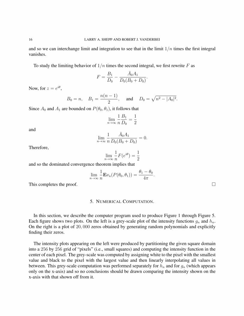
In this section, we describe the computer program used to produce Figure 1 through Figure 5.Each figure shows two plots. On the left is a grey-scale plot of the intensity functions gn and hn.On the right is a plot of 20, 000 zeros obtained by generating random polynomials and explicitlyfinding their zeros.

The intensity plots appearing on the left were produced by partitioning the given square domaininto a 256 by 256 grid of “pixels” (i.e., small squares) and computing the intensity function in thecenter of each pixel. The grey-scale was computed by assigning white to the pixel with the smallestvalue and black to the pixel with the largest value and then linearly interpolating all values inbetween. This grey-scale computation was performed separately for hn and for gn (which appearsonly on the x-axis) and so no conclusions should be drawn comparing the intensity shown on thex-axis with that shown off from it.


FIGURE 1. Random quadratics (n = 3). In this figure and the next several, theleft-hand plot is a grey-scale image of the intensity functions hn and gn (which isconcentrated on the x-axis). The right-hand plot shows 20, 000 roots from randomlygenerated polynomials. Subsequent captions give more information pertaining toeach of these figures.

Of course, the intensity function gn is one-dimensional and therefore it would be natural (andmore informative) to make separate plots of values of gn verses x, but such plots appear in manyplaces (see, e.g., [8]) and so it seemed unnecessary to produce them here. Suffice it to say that gnis a density whose mass lies primarily near ±1.

The 20, 000 zeros plotted on the right were produced by a novel root finding algorithm, whichwe shall describe briefly. Given a polynomial P , the algorithm that finds its zeros in a given squareR is recursive. Let S denote the smallest disk that contains R. Using the argument principle, wecan compute the number of zeros in S:

(5.1) ν(S) =1

2πi

∫∂S

P ′(z)

P (z)dz.

If ν(S) is zero, then we stop since there are then no zeros in R. Otherwise, we compute the sumof the zeros using the following analogue of the argument principle:

(5.2) σ(S) =∑i:zi∈S

zi =1

2πi

∫∂S

zP ′(z)

P (z)dz.


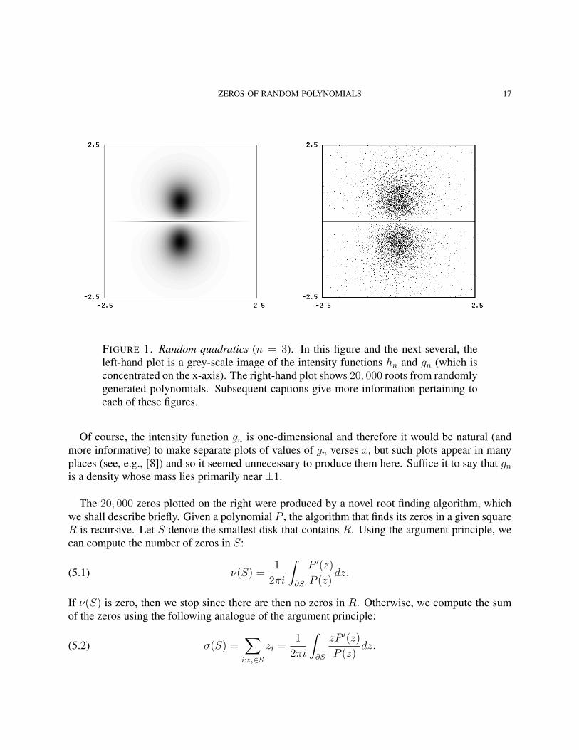
FIGURE 2. Random cubics (n = 4). Note that, for the left-hand plots, the grey-scales for hn and gn are produced separately and in such a way that both use the fullrange from white to black.

Here, the zi’s denote the zeros of P . The ratio

α(S) = σ(S)/ν(S)

is then the barycenter of the zeros contained in S (counting multiplicities). Next, let B be a diskof very small radius centered at α(S) and again using the argument principle we count the numberof zeros in this disk. If this number equals ν(S), then there is only one zero in S, it is at α(S) andit has multiplicity ν(S). Hence, again we stop (but first, we check whether the zero is in fact in Rand if it is, we add it to our list of zeros found so far). In all other cases, there are still two or morezeros to be found and so we partition the square into four subsquares and recursively call this sameprocedure on those subsquares. Except for discussing how to compute the contour integrals, thisis a complete description of the algorithm used to produce the right-hand plots.

The contour integrals in (5.1) and (5.2) are computed as follows. First we compute ν(S). Todo this, we begin by simply using a discrete approximation to the integral consisting of 8 pointsspread equally around the boundary of S. Then we check to see if ν(S) is close to being an integer.If it is, we are done. If it isn’t, then we spread 8 more points midway between each point alreadyused in the sum and we update the sum with these points. Again we check nearness to integrality.We continue in this way until the integrality condition is satisfied. The contour integral in (5.2) isthen computed using the same number of points as was used in (5.1).


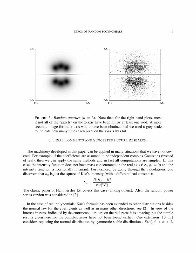
FIGURE 3. Random quartics (n = 5). Note that, for the right-hand plots, mostif not all of the “pixels” on the x-axis have been hit by at least one root. A moreaccurate image for the x-axis would have been obtained had we used a grey-scaleto indicate how many times each pixel on the x-axis was hit.

6. FINAL COMMENTS AND SUGGESTED FUTURE RESEARCH.

The machinery developed in this paper can be applied in many situations that we have not cov-ered. For example, if the coefficients are assumed to be independent complex Gaussains (insteadof real), then we can apply the same methods and in fact all computations are simpler. In thiscase, the intensity function does not have mass concentrated on the real axis (i.e., gn = 0) and theintensity function is rotationally invariant. Furthermore, by going through the calculations, onediscovers that hn is just the square of Kac’s intensity (with a different lead constant):

hn =B0B2 −B2

1

π|z|2B20

.

The classic paper of Hammersley [5] covers this case (among others). Also, the random powerseries version was considered in [3].

In the case of real polynomials, Kac’s formula has been extended to other distributions besidesthe normal law for the coefficients as well as in many other directions, see [2]. In view of theinterest in zeros indicated by the enormous literature on the real zeros it is amazing that the simpleresults given here for the complex zeros have not been found earlier. One extension [10, 11]considers replacing the normal distribution by symmetric stable distributions, S(α), 0 < α < 2,


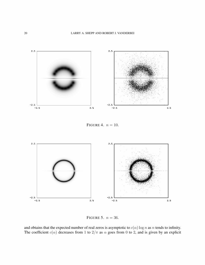
FIGURE 4. n = 10.

FIGURE 5. n = 36.

and obtains that the expected number of real zeros is asymptotic to c(α) log n as n tends to infinity.The coefficient c(α) decreases from 1 to 2/π as α goes from 0 to 2, and is given by an explicit


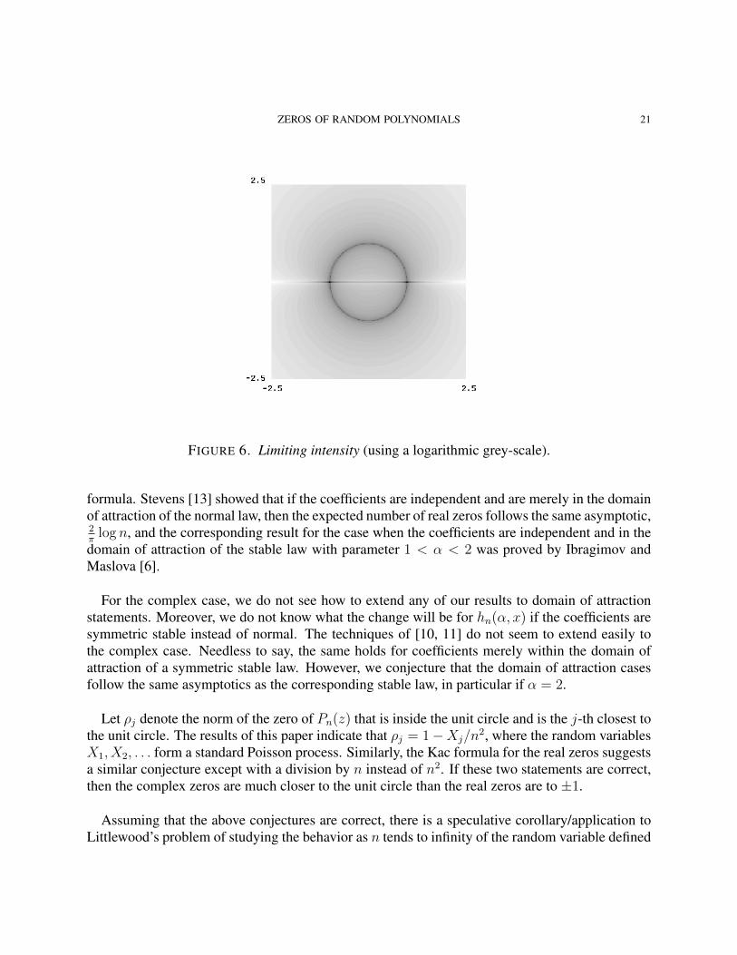
FIGURE 6. Limiting intensity (using a logarithmic grey-scale).

formula. Stevens [13] showed that if the coefficients are independent and are merely in the domainof attraction of the normal law, then the expected number of real zeros follows the same asymptotic,2π

log n, and the corresponding result for the case when the coefficients are independent and in thedomain of attraction of the stable law with parameter 1 < α < 2 was proved by Ibragimov andMaslova [6].

For the complex case, we do not see how to extend any of our results to domain of attractionstatements. Moreover, we do not know what the change will be for hn(α, x) if the coefficients aresymmetric stable instead of normal. The techniques of [10, 11] do not seem to extend easily tothe complex case. Needless to say, the same holds for coefficients merely within the domain ofattraction of a symmetric stable law. However, we conjecture that the domain of attraction casesfollow the same asymptotics as the corresponding stable law, in particular if α = 2.

Let ρj denote the norm of the zero of Pn(z) that is inside the unit circle and is the j-th closest tothe unit circle. The results of this paper indicate that ρj = 1−Xj/n

2, where the random variablesX1, X2, . . . form a standard Poisson process. Similarly, the Kac formula for the real zeros suggestsa similar conjecture except with a division by n instead of n2. If these two statements are correct,then the complex zeros are much closer to the unit circle than the real zeros are to ±1.

Assuming that the above conjectures are correct, there is a speculative corollary/application toLittlewood’s problem of studying the behavior as n tends to infinity of the random variable defined


as

(6.1) mn = inf0≤θ≤2π

∣∣Pn(eiθ)∣∣ ,

i.e., the infimum on the unit circle of Pn(z). Here, the coefficients are assumed to be independentsymmetric ±1 random variables. Konyagin gave a new estimate for mn in [9] by a rather com-plicated argument. We cannot obtain his delicate estimate by our methods, but there is at leastsome hope that this can be done provided that some further developments can be carried out. Onewould have to prove that the conjecture that the nearest complex zero to the unit circle is withinO(1/n2) holds not only for normal coefficients but for +-1 coefficients. As pointed out privately byA.M. Odlyzko, it would then follow from Bernstein’s theorem that an alternate proof to Konyagin’sestimates in [9] would be obtainable.

Acknowledgement 6.1. The results of this paper and our resulting speculations on finding an alter-nate proof based on studying the zeros of Pn(z) near the unit circle were stimulated by a talk byS.V. Konyagin. In the course of these speculations, the study of the zeros themselves began to beeven more interesting to us that the application to Littlewood’s problem. The application will haveto await further inspiration and another paper (possibly by other authors).

We would also like to acknowledge Ofer Zeitouni for carefully reading an early draft of thepaper and suggesting some important algebraic simplifications.

REFERENCES

1. L.V. Ahlfors, Complex analysis, McGraw-Hill, New York, NY, 1966.2. A.T. Bharucha-Reid and M. Sambandham, Random polynomials, Academic Press, 1986.3. A. Edelman and E. Kostlan, How many zeros of a random polynomial are real?, J. AMS (1995), To appear.4. P. Erdos and P. Turan, On the distribution of roots of polynomials, Ann. Math. 51 (1950), 105–119.5. J. Hammersley, The zeros of a random polynomial, Proc. Third Berkeley Symp. Math. Stat. Probability, vol. 2,

1956, pp. 89–111.6. I.A. Ibragimov and N.B. Maslova, On the expected number of real zeros of random polynomials. i. coefficients

with zero means, Teor. Veroyatn. Ee Primen. 16 (1971), 229–248.7. M. Kac, On the average number of real roots of a random algebraic equation, Bull. Amer. Math. Soc. 49 (1943),

314–320,938.8. , Probability and related topics in physical sciences, Interscience, London, 1959.9. S.V. Konyagin, On minimum of modulus of random trigonometric oolynomials with coefficients ±1, Matem.

zametki 56 (1994), 80–101, In Russian.10. B.F. Logan and L.A. Shepp, Real zeros of random polynomials, Proc. London Math. Soc. Third Series 18 (1968),

29–35.11. , Real zeros of random polynomials ii, Proc. London Math. Soc. Third Series 18 (1968), 308–314.12. S.O. Rice, Mathematical theory of random noise, Bell System Tech. J. 25 (1945), 46–156.13. D.C. Stevens, The average and variance of the number of real zeros of random functions, Ph.D. Dissertation, New

York University, New York, 1965.14. D.I. Sparo and M.G. Sur, On the distribution of roots of random polynomials, Vestn. Mosk. Univ., Ser. 1: Mat.,

Mekh. (1962), 40–53.


LARRY A. SHEPP, AT&T BELL LABORATORIES, MURRAY HILL, NJ 07974

E-mail address: [email protected]

ROBERT J. VANDERBEI, PROGRAM IN STATISTICS AND OPERATIONS RESEARCH, PRINCETON UNIVERSITY,PRINCETON, NJ 08544

E-mail address: [email protected]

The Complex Zeros of Random Polynomials. - Princeton University

Documents

Transcript of The Complex Zeros of Random Polynomials. - Princeton University