11 Interconnected Systems

A positive system Σ with input u{t) and output y(t) is often composed of q inter-connected positive subsystems Ej with input i/j(t) and output Zj(£). If the system is discrete-time, each subsystem E¿ is described by the equations

Xi{t + 1) = AiXi(t) + biVi(t) (11.1)

zi{t) = cjxi{t) (11.2)

where x¿(t) 6 Rní,i/¿(í) G R and z¿(í) e R. The interconnections define the dependency of the input i>i(t) of each Ej upon

the outputs zi(t), Zi(t),..., zq(t) of the subsystems and upon the input u(t) of Σ, as well as the dependency of the output y(t) of Σ upon the outputs ζ,·(ί) of the subsystems Σ«. In other words, letting

V(t) = (u1(t) V2(t) ... Vq{t))T

z(t) = (Zl(t) z2(t) . . . zg(t))T

one has

v(t) = ílz(t) + 7ti(í) (11.3)

y{t) = VTz(t) (11.4)

where Ω in a q x q matrix and 7 and Φ are g-dimensional vectors. The triplet (Ω, 7, Φ τ ) can be represented by means of a graph, called the interconnection graph.

101

Positive Linear Systems: Theory and Applications by Lorenzo Farina and Sergio Rinaldi

Copyright © 2000 John Wiley & Sons, Inc.

102 INTERCONNECTED SYSTEMS

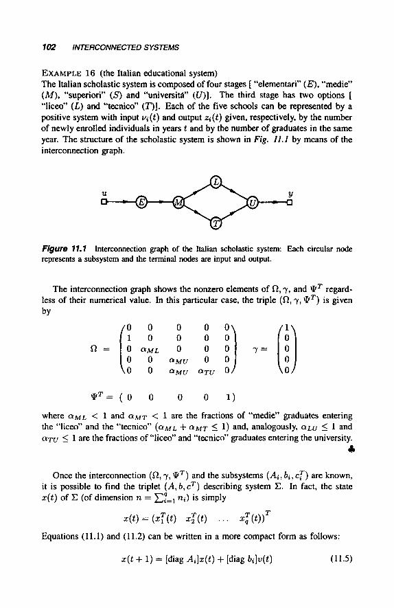
EXAMPLE 16 (the Italian educational system) The Italian scholastic system is composed of four stages [ "elementan" (E), "medie" (M), "superiori" (S) and "universitá" (Í/)]· The third stage has two options [ "liceo" (L) and "técnico" (T)]· Each of the five schools can be represented by a positive system with input f¿(t) and output Zj(i) given, respectively, by the number of newly enrolled individuals in years t and by the number of graduates in the same year. The structure of the scholastic system is shown in Fig. 11.1 by means of the interconnection graph.

Figure 11.1 Interconnection graph of the Italian scholastic system: Each circular node represents a subsystem and the terminal nodes are input and output.

The interconnection graph shows the nonzero elements of Ω, 7, and Φ τ regard-less of their numerical value. In this particular case, the triple (Ω, 7, Φ τ ) is given by

Ω = f°

0 0

\ 0

0 0

<*ML

0 0

0 0 0

O-MU

<*MU

0 0 0 0

aTu

0 0 0 0)

7 = CA

0 0

Φ3 ( 0 0 0 0 1)

where CIML < 1 and OMT < 1 are the fractions of "medie" graduates entering the "liceo" and the "técnico" (CXML + (*MT < 1) and, analogously, am < 1 and αχυ ^ 1 are the fractions of "liceo" and "técnico" graduates entering the university.

Once the interconnection (Ω, 7, Φ τ ) and the subsystems (Ai} 6i; cf) are known, it is possible to find the triplet (A, b, cT) describing system Σ. In fact, the state x(t) of Σ (of dimension n = £ ] ' = 1

n<) ' s simply

x(t) = (xj(t) xZ(t) . . . xTq{t)f

Equations (11.1) and (11.2) can be written in a more compact form as follows:

x(t + 1) = [diag Ai]x(t) + [diag bi]v(t) (11.5)

PROPERTIES 103

z(t) = [diag cf]x{t) (11.6)

where [Ai ] is a matrix of matrices having on its diagonal the matrices A\, A<i,..., Aq

and zeros elsewhere, while [diag 6J and [diag cf ] are matrices of (column and row) vectors with nonzero vectors (6¿ and cf) on their diagonal. If we take into account (11.3), (11.4), (11.5), and (11.6), we can obtain the state equations and the output transformation of system Σ

x(t + l) = Ax(t)+bu(t)

y(t) = cTx(t)

and it is readily seen that

A = [diag Ai] + [diag 6¿]n[diag cf]

b = [diag &ift

CT _ tyTfdiag CT)

Moreover, if the subsystems are positively interconnected, that is, if Ω7 and Φ τ

are nonnegative, system Σ is a positive system. In the sequel, we will refer to this class of interconnected systems.

In order to discuss the properties of an interconnected system, one could first compute the triplet (A, b, cT), and then apply to it the methods described in the previous chapters. However, by doing so, one would not take any advantage from the specific structure of the interconnections. In some cases, it is possible to derive a number of properties of the interconnected system by studying only the analogous properties of its subsystems. When this happens, there is often a great advantage since it is generally easier to study the properties of q matrices (Ai) of dimensions rii x rii, than the analogous property of a single matrix A of dimensions nxn with

n = Σ?=ι η>· A first property, concerning the stability of the interconnections of positive sys-

tems, is Theorem 36.

THEOREM 36 (asymptotically stable interconnected systems)

If an interconnected system Σ is asymptotically stable, then all its subsystems Σί are asymptotically stable.

Proof. The proof is a straightforward consequence of the fact, previously described, that asymptotically stable positive systems are connectively stable.

It is worth noting that Theorem 36 is false for nonpositive linear systems. For example, an unstable system can be stabilized using a feedback scheme. By contrast, an unstable positive system cannot be stabilized by positively interconnecting it with

104 INTERCONNECTED SYSTEMS

other positive systems. In particular, an unstable positive system (.A, b, cT) cannot be stabilized using an algebraic linear control law

u(t) = kiii(t) + A;2X2(i) H l· knxn(t)

if the gains ki are constrained to be nonnegative [in order to guarantee that u(£) is nonnegative].

An analogous property (Theorem 37) holds for excitability.

THEOREM 37 (excitable interconnected systems)

If an interconnected system Σ is excitable, then all its subsystems E¿ are ex-citable.

Proof. If Σ is excitable there exists a nonnegative input that brings the system from the origin x(0) = 0 to a strictly positive state in a finite time interval T. Since x(T) = (xf (Γ) xl{T) ... xj(T))T, then x¿(T) » 0, i = 1 ,2 , . . . , q. This implies that each subsystem E¿ initially at rest, has been transferred to a strictly positive state in finite time. Thus, each subsystem E¿ is excitable.

0

For interconnected systems that are asymptotically stable and excitable (i.e., standard), both Theorems 36 and 37 hold so that Theorem 38 holds.

THEOREM 38 (standard interconnected systems)

If an interconnected system Σ is standard, then all its subsystems Σ< are stan-dard.

The following result (Theorem 39), which extends Theorem 35, concerns the minimum phase of interconnected positive systems.

THEOREM 39 (condition for minimum phase)

An asymptotically stable interconnected system Σ with an interconnection graph containing a unique direct input-output path, is minimum phase if and only if all the subsystems E¿ composing such a path are minimum phase.

Proof. Denote by 1 ,2 , . . . , q the subsystems composing the unique direct input-output path of the interconnection graph and by Fi(p) their transfer functions. Following the same procedure used in the proof of Theorem 35, it is possible to construct an interconnected system of the type shown in Fig. 10.1 having the same transfer function of Σ. Then, all the subsystems of the block diagram in Fig. 10.1 are externally stable, since Σ is connectively stable (being asymptotically stable), while all the subsystems composing the direct input-output path are, by assumption, minimum phase. Consequently, a and b used in the proof of Theorem 35 are fulfilled and we can conclude, through the same reasoning, that the system is minimum phase. On the other hand, it is easy to check that if the transfer function

PROPERTIES 105

of the system has no unstable zeros, the transfer functions Fi(p) must be minimum phase.

0

Example 17 illustrates how Theorem 39 can be fruitfully exploited to show that a system is minimum phase.

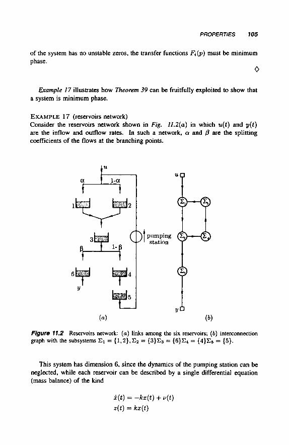
EXAMPLE 17 (reservoirs network) Consider the reservoirs network shown in Fig. 11.2(a) in which u(t) and y(t) are the inflow and outflow rates. In such a network, a and ß are the splitting coefficients of the flows at the branching points.

a 1-a u n

©—®

C^) I Pumping ( ξ ν — / Ώ v . ^ 1 station ΊΓ ^ - '

(a) (6)

Figure 11.2 Reservoirs network: (a) links among the six reservoirs; (6) interconnection graph with the subsystems Σι = {1,2},Σ2 = {3}Σ3 = {6}Σ4 = {4}Σ5 = {5}.

This system has dimension 6, since the dynamics of the pumping station can be neglected, while each reservoir can be described by a single differential equation (mass balance) of the kind

x(t) = -kx(t) + u(t)

z(t) = kx{t)

106 INTERCONNECTED SYSTEMS

where x(t) is the water storage and k is the ratio between outflow rate z(t) and storage.

Theorem 35 is not applicable, since the influence graph of the system, which is not shown, contains two direct input-output paths (the water can flow directly from the input to the output through the reservoirs 1,3,6 or 2,3,6).

We could therefore determine the triplet (A, b, cT) describing the whole system and explicitly evaluate its transfer function in order to check whether its zeros have a negative real part. The reader is invited to perform these calculations in order to better appreciate the following considerations, based on Theorem 39.

By grouping reservoirs 1 and 2 together into a single subsystem Σι and con-sidering each of the remaining reservoirs as a subsystem, the network depicted in Fig. 11.2(a) is described by the interconnection graph of Fig. 11.2(b) in which Σι = {1,2},Σ2 = {3},Σ3 = {6},Σ4 = {4},Σ5 = {5}. Since in such a graph there exists a unique direct input-output path and since the system is, for obvious physical reasons, asymptotically stable, we can apply Theorem 39, which states that the system is minimum phase if and only if the three subsystems Σι , Σ2, and Σ3 composing the direct path are minimum phase. Two of these subsystems (Σ2 and Σ3 ) are single reservoirs, that is, first-order linear systems that do not have zeros and are, therefore, minimum phase. Thus, we must only check whether subsystem Σι , composed of reservoirs 1 and 2, is minimum phase or not. Since the transfer function of a single reservoir is

G(s) s + k

subsystem Σ ι , composed by the parallel connection of reservoirs 1 and 2 with splitting coefficient a , has the transfer function

&! k2 [aki + (1 -a)k2}3 + k1k2 Fi(s) = a ;—h (1 - a) — = . , . .—-r-r w s + k! K 's + k2 (s + k^s + fa)

The zero of the transfer function Fi(s) is negative for all values of the splitting coefficient a. We can then conclude that Σι is minimum phase, so that, thanks to Theorem 39, the whole network is minimum phase for every value of the splitting coefficients a and β.

*