Seshadri Constants and Fujita’s Conjecture viaPositive Characteristic Methods

by

Takumi Murayama

A dissertation submitted in partial fulfillmentof the requirements for the degree of

Doctor of Philosophy(Mathematics)

in the University of Michigan2019

Doctoral Committee:

Professor Mircea Mustata, ChairProfessor Ratindranath AkhouryProfessor Melvin HochsterProfessor Mattias JonssonProfessor Karen E. Smith

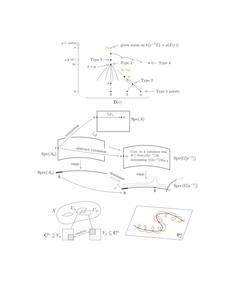
x0

x ∨ y

0 b a

Type 2

Type 1 points

Type 2

given norm on kr−1T = p(E(r))

Type 3

ρ = radius

r

0

ρ /∈ |k∗||a|

D(r)

Type 4

y

x

[y, x0]

aa−1

· · ·Spec(G[a−1])

pq

Spv(G[a−1])

supp

sCorr. to a valuation ringR ⊂ Frac(G[a−1]/q)

dominating (G[a−1]/q)p/q

Spv(Aa)

t abstract extension

dominant

Spec(Aa)

supp

q

Spv(A)

⊆

u

restriction

v·|cΓu

XUα Uβ

analytic

Cn ⊇ VαVβ ⊆ Cn

P2k

p

Takumi Murayama

takumim@umich.edu

ORCID iD: 0000-0002-8404-8540

c© Takumi Murayama 2019

To my family

ii

Acknowledgments

First of all, I am tremendously grateful to my advisor Mircea Mustata for his constant

support throughout the last five years. I learned much of the philosophy and many of

the methods behind the results in this thesis from him, and I am very thankful for his

patience and guidance as I worked out the many moving pieces that came together to

become this thesis.

I would also like to thank the rest of my doctoral committee. I have benefited greatly

from taking courses from Ratindranath Akhoury, Melvin Hochster, Mattias Jonsson,

and Karen E. Smith, and I am especially glad that they are willing to discuss physics

or mathematics with me when I have questions about their work or the classes they

are teaching. My intellectual debt to Mel and Karen is particularly apparent in this

thesis, since much of the underlying commutative-algebraic theory was developed by Mel

and his collaborators, and this theory was first applied to algebraic geometry by Karen

among others. I would also like to thank Bhargav Bhatt, from whom I also learned a lot

of mathematics through courses and in the seminars that he often led.

Next, I would like to thank my collaborators Rankeya Datta, Yajnaseni Dutta, Mihai

Fulger, Jeffrey C. Lagarias, Lance E. Miller, David Harry Richman, and Jakub Witaszek

for their willingness to work on mathematics with me. While only some of our joint work

appears explicitly in this thesis, the ideas I learned through conversations with them

have had a substantial impact on the work presented here.

I would also like to extend my gratitude toward my fellow colleagues at Michigan for

many useful conversations, including (but not limited to) Harold Blum, Eric Canton,

Francesca Gandini, Jack Jeffries, Zhan Jiang, Hyung Kyu Jun, Devlin Mallory, Eamon

Quinlan-Gallego, Ashwath Rabindranath, Emanuel Reinecke, Matthew Stevenson, Robert

M. Walker, Rachel Webb, and Ming Zhang. I am particularly grateful to Farrah Yhee,

without whose support I would have had a much harder and definitely more stressful

time as a graduate student. I would also like to thank Javier Carvajal-Rojas, Alessandro

iii

De Stefani, Lawrence Ein, Krishna Hanumanthu, Mitsuyasu Hashimoto, Janos Kollar,

Alex Kuronya, Yuchen Liu, Linquan Ma, Zsolt Patakfalvi, Thomas Polstra, Mihnea

Popa, Kenta Sato, Karl Schwede, Junchao Shentu, Daniel Smolkin, Shunsuke Takagi,

Hiromu Tanaka, Kevin Tucker, and Ziquan Zhuang for helpful discussions about material

in this thesis through the years.

Finally, I would like to thank my parents, sisters, grandparents, and other relatives

for their constant support throughout my life. They have always been supportive of me

working in mathematics, and of my career and life choices. I hope that my grandparents

in particular are proud of me, even though all of them probably have no idea what I

work on, and some of them did not have the chance to witness me receiving my Ph.D.

This material is based upon work supported by the National Science Foundation under

Grant Nos. DMS-1265256 and DMS-1501461.

iv

Table of Contents

Dedication ii

Acknowledgments iii

List of Figures viii

List of Tables ix

List of Appendices x

List of Symbols xi

Abstract xiv

Chapter 1. Introduction 11.1. Outline . . . . . . . . . . . . . . . . . . . . . . . . . . . . . . . . . . . . 91.2. Notation and conventions . . . . . . . . . . . . . . . . . . . . . . . . . 10

Chapter 2. Motivation and examples 112.1. Fujita’s conjecture . . . . . . . . . . . . . . . . . . . . . . . . . . . . . 112.2. Seshadri constants . . . . . . . . . . . . . . . . . . . . . . . . . . . . . 162.3. A relative Fujita-type conjecture . . . . . . . . . . . . . . . . . . . . . . 232.4. Difficulties in positive characteristic . . . . . . . . . . . . . . . . . . . . 24

2.4.1. Proof of Theorem B . . . . . . . . . . . . . . . . . . . . . . . . 252.4.2. Raynaud’s counterexample to Kodaira vanishing . . . . . . . . . 30

Chapter 3. Characterizations of projective space 363.1. Background . . . . . . . . . . . . . . . . . . . . . . . . . . . . . . . . . 373.2. Proof of Theorem A . . . . . . . . . . . . . . . . . . . . . . . . . . . . 41

Chapter 4. Preliminaries in arbitrary characteristic 464.1. Morphisms essentially of finite type . . . . . . . . . . . . . . . . . . . . 464.2. Cartier and Weil divisors . . . . . . . . . . . . . . . . . . . . . . . . . . 494.3. Reflexive sheaves . . . . . . . . . . . . . . . . . . . . . . . . . . . . . . 51

v

4.4. Dualizing complexes and Grothendieck duality . . . . . . . . . . . . . . 524.5. Base ideals and base loci . . . . . . . . . . . . . . . . . . . . . . . . . . 534.6. Asymptotic invariants of line bundles . . . . . . . . . . . . . . . . . . . 55

4.6.1. Stable base loci . . . . . . . . . . . . . . . . . . . . . . . . . . . 554.6.2. Augmented base loci . . . . . . . . . . . . . . . . . . . . . . . . 564.6.3. Asymptotic cohomological functions . . . . . . . . . . . . . . . . 594.6.4. Restricted volumes . . . . . . . . . . . . . . . . . . . . . . . . . 61

4.7. Log pairs and log triples . . . . . . . . . . . . . . . . . . . . . . . . . . 624.8. Singularities of pairs and triples . . . . . . . . . . . . . . . . . . . . . . 62

4.8.1. Log canonical thresholds . . . . . . . . . . . . . . . . . . . . . . 644.9. Multiplier ideals . . . . . . . . . . . . . . . . . . . . . . . . . . . . . . . 66

Chapter 5. Preliminaries in positive characteristic 705.1. Conventions on the Frobenius morphism . . . . . . . . . . . . . . . . . 705.2. The pigeonhole principle . . . . . . . . . . . . . . . . . . . . . . . . . . 715.3. F -finite schemes . . . . . . . . . . . . . . . . . . . . . . . . . . . . . . . 735.4. F -singularities of pairs and triples . . . . . . . . . . . . . . . . . . . . . 74

5.4.1. The trace of Frobenius . . . . . . . . . . . . . . . . . . . . . . . 775.4.2. F -pure thresholds . . . . . . . . . . . . . . . . . . . . . . . . . . 80

5.5. Test ideals . . . . . . . . . . . . . . . . . . . . . . . . . . . . . . . . . . 815.6. Reduction modulo p . . . . . . . . . . . . . . . . . . . . . . . . . . . . 89

5.6.1. Singularities vs. F -singularities . . . . . . . . . . . . . . . . . . 93

Chapter 6. The ampleness criterion of de Fernex–Kuronya–Lazarsfeld 966.1. Motivation and statement . . . . . . . . . . . . . . . . . . . . . . . . . 976.2. A lemma on base loci . . . . . . . . . . . . . . . . . . . . . . . . . . . . 996.3. Proof of Theorem E . . . . . . . . . . . . . . . . . . . . . . . . . . . . . 105

Chapter 7. Moving Seshadri constants 1117.1. Definition and basic properties . . . . . . . . . . . . . . . . . . . . . . . 1117.2. Alternative descriptions . . . . . . . . . . . . . . . . . . . . . . . . . . 113

7.2.1. Nakamaye’s description . . . . . . . . . . . . . . . . . . . . . . . 1147.2.2. A description in terms of jet separation . . . . . . . . . . . . . . 116

7.3. A generalization of Theorem B . . . . . . . . . . . . . . . . . . . . . . . 1277.3.1. Proof in positive characteristic . . . . . . . . . . . . . . . . . . . 1287.3.2. Proof in characteristic zero . . . . . . . . . . . . . . . . . . . . . 133

Chapter 8. The Angehrn–Siu theorem 1388.1. The lifting theorem . . . . . . . . . . . . . . . . . . . . . . . . . . . . . 1398.2. Constructing singular divisors and proof of Theorem D . . . . . . . . . 145

vi

Appendices 155

Bibliography 173

vii

List of Figures

1.1. Raphael’s School of Athens (1509–1511) . . . . . . . . . . . . . . . . . . . 21.2. Kobe Port Tower in the Kobe harbor (2006) . . . . . . . . . . . . . . . . . 3

2.1. Kollar’s example (Example 2.1.6) . . . . . . . . . . . . . . . . . . . . . . . 132.2. Computing the Seshadri constant of the hyperplane class on Pn

k . . . . . . 172.3. Miranda’s example (Example 2.2.9) . . . . . . . . . . . . . . . . . . . . . . 212.4. Raynaud’s example (Example 2.4.4) . . . . . . . . . . . . . . . . . . . . . . 32

3.1. Mori’s characterization of Pnk . . . . . . . . . . . . . . . . . . . . . . . . . 38

4.1. Log resolution of a cuspidal cubic . . . . . . . . . . . . . . . . . . . . . . . 66

5.1. Singularities vs. F -singularities . . . . . . . . . . . . . . . . . . . . . . . . 94

6.1. Asymptotic cohomological functions on an abelian surface . . . . . . . . . 986.2. Hypercohomology spectral sequence computing Hj(X,OX(mL− rA)) . . . 109

A.1. Relationships between different classes of F -singularities . . . . . . . . . . 161

viii

List of Tables

2.1. Known cases of Fujita’s freeness conjecture over the complex numbers . . . 16

5.1. Some properties preserved under spreading out . . . . . . . . . . . . . . . 915.2. Some properties preserved under reduction modulo p . . . . . . . . . . . . 93

A.1. Proofs of relationships between different classes of F -singularities . . . . . 162

ix

List of Appendices

Appendix A. F -singularities for non-F -finite rings 155

Appendix B. The gamma construction of Hochster–Huneke 163B.1. Construction and main result . . . . . . . . . . . . . . . . . . . . . . . 163B.2. Applications . . . . . . . . . . . . . . . . . . . . . . . . . . . . . . . . 170

B.2.1. Openness of F -singularities . . . . . . . . . . . . . . . . . . . . 170B.2.2. F -singularities for rings essentially of finite type . . . . . . . . 171

x

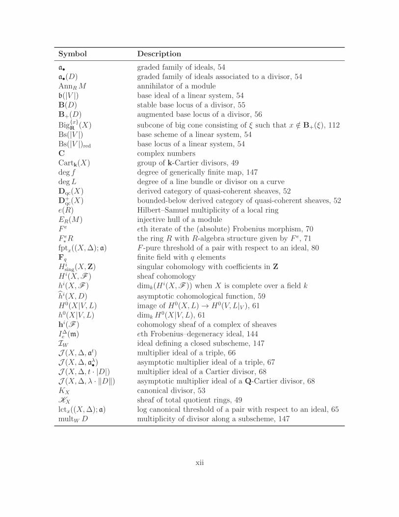
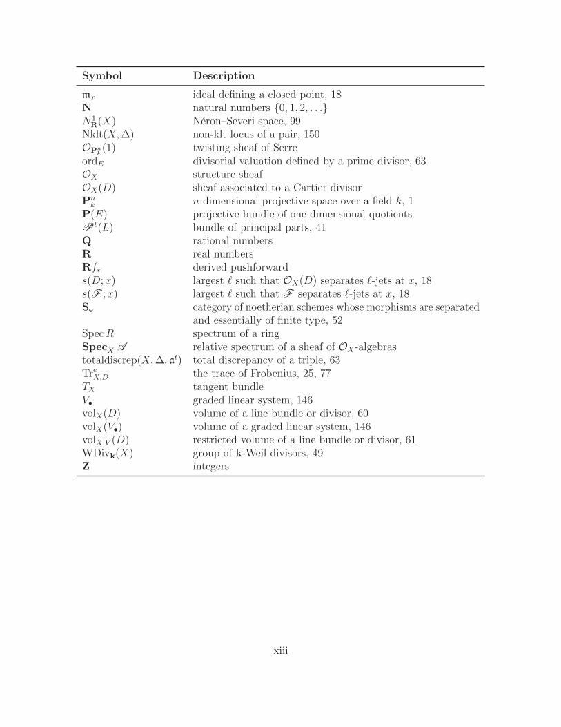
List of Symbols

Symbols are grouped into three groups, depending on whether they start with punctuation,Greek letters, or Latin letters.

Symbol Description

(−)! exceptional pullback of Grothendieck duality, 52(−)∗(−) tight closure, 88, 155

(−)[pe] eth Frobenius power of an ideal or module, 71, 88(−) complement of the union of minimal primes in a ring, 62(−)∨ dual of a sheaf, 51≡k k-numerical equivalence∼k k-linear equivalence(LdimV · V ) intersection product, 10(X,∆, aλ•) log triple, 62dDe round-up of a divisor, 50bDc round-down of a divisor, 50|D| complete linear system, 54|V | linear system, 54ε(D;x) Seshadri constant, 17ε(‖D‖;x) moving Seshadri constant, 111εjet(‖D‖;x) jet separation description for ε(‖D‖;x), 117εN(‖D‖;x) Nakamaye’s description for ε(‖D‖;x), 114ε`F (D;x) `th Frobenius–Seshadri constant, 132ε∆F -sig(D;x) F -signature Seshadri constant, 144τ(X,∆, at) test ideal of a triple, 82, 84τ(X,∆, aλ•) asymptotic test ideal of a triple, 87τ(X,∆, t · |D|) test ideal of a Cartier divisor, 87τ(X,∆, λ · ‖D‖) asymptotic test ideal of a Q-Cartier divisor, 88ΩX cotangent bundleωX canonical bundle or sheaf, 53ω•X (normalized) dualizing complex, 53a(E,X,∆, at) discrepancy of E with respect to a triple, 63

xi

Symbol Description

a• graded family of ideals, 54a•(D) graded family of ideals associated to a divisor, 54AnnRM annihilator of a moduleb(|V |) base ideal of a linear system, 54B(D) stable base locus of a divisor, 55B+(D) augmented base locus of a divisor, 56

BigxR (X) subcone of big cone consisting of ξ such that x /∈ B+(ξ), 112

Bs(|V |) base scheme of a linear system, 54Bs(|V |)red base locus of a linear system, 54C complex numbersCartk(X) group of k-Cartier divisors, 49deg f degree of generically finite map, 147degL degree of a line bundle or divisor on a curveDqc(X) derived category of quasi-coherent sheaves, 52D+

qc(X) bounded-below derived category of quasi-coherent sheaves, 52e(R) Hilbert–Samuel multiplicity of a local ringER(M) injective hull of a moduleF e eth iterate of the (absolute) Frobenius morphism, 70F e∗R the ring R with R-algebra structure given by F e, 71

fptx((X,∆); a) F -pure threshold of a pair with respect to an ideal, 80Fq finite field with q elementsH i

sing(X,Z) singular cohomology with coefficients in ZH i(X,F ) sheaf cohomologyhi(X,F ) dimk(H

i(X,F )) when X is complete over a field k

hi(X,D) asymptotic cohomological function, 59H0(X|V, L) image of H0(X,L)→ H0(V, L|V ), 61h0(X|V, L) dimkH

0(X|V, L), 61hi(F ) cohomology sheaf of a complex of sheavesI∆e (m) eth Frobenius–degeneracy ideal, 144IW ideal defining a closed subscheme, 147J (X,∆, at) multiplier ideal of a triple, 66J (X,∆, aλ•) asymptotic multiplier ideal of a triple, 67J (X,∆, t · |D|) multiplier ideal of a Cartier divisor, 68J (X,∆, λ · ‖D‖) asymptotic multiplier ideal of a Q-Cartier divisor, 68KX canonical divisor, 53KX sheaf of total quotient rings, 49lctx((X,∆); a) log canonical threshold of a pair with respect to an ideal, 65multW D multiplicity of divisor along a subscheme, 147

xii

Symbol Description

mx ideal defining a closed point, 18N natural numbers 0, 1, 2, . . .N1

R(X) Neron–Severi space, 99Nklt(X,∆) non-klt locus of a pair, 150OPnk

(1) twisting sheaf of SerreordE divisorial valuation defined by a prime divisor, 63OX structure sheafOX(D) sheaf associated to a Cartier divisorPnk n-dimensional projective space over a field k, 1

P(E) projective bundle of one-dimensional quotientsP`(L) bundle of principal parts, 41Q rational numbersR real numbersRf∗ derived pushforwards(D;x) largest ` such that OX(D) separates `-jets at x, 18s(F ;x) largest ` such that F separates `-jets at x, 18Se category of noetherian schemes whose morphisms are separated

and essentially of finite type, 52SpecR spectrum of a ringSpecX A relative spectrum of a sheaf of OX-algebrastotaldiscrep(X,∆, at) total discrepancy of a triple, 63TreX,D the trace of Frobenius, 25, 77TX tangent bundleV• graded linear system, 146volX(D) volume of a line bundle or divisor, 60volX(V•) volume of a graded linear system, 146volX|V (D) restricted volume of a line bundle or divisor, 61WDivk(X) group of k-Weil divisors, 49Z integers

xiii

Abstract

In 1988, Fujita conjectured that there is an effective and uniform way to turn an ample line

bundle on a smooth projective variety into a globally generated or very ample line bundle.

We study Fujita’s conjecture using Seshadri constants, which were first introduced by

Demailly in 1992 with the hope that they could be used to prove cases of Fujita’s

conjecture. While examples of Miranda seemed to indicate that Seshadri constants could

not be used to prove Fujita’s conjecture, we present a new approach to Fujita’s conjecture

using Seshadri constants and positive characteristic methods. Our technique recovers

some known results toward Fujita’s conjecture over the complex numbers, without the

use of vanishing theorems, and proves new results for complex varieties with singularities.

Instead of vanishing theorems, we use positive characteristic techniques related to the

Frobenius–Seshadri constants introduced by Mustata–Schwede and the author. As an

application of our results, we give a characterization of projective space using Seshadri

constants in positive characteristic, which was proved in characteristic zero by Bauer

and Szemberg.

xiv

Chapter 1

Introduction

Algebraic geometry is the study of algebraic varieties, which are geometric spaces defined

by polynomial equations. Some varieties are particularly simple, and the simplest

algebraic varieties are perhaps the n-dimensional projective spaces Pnk . Recall that if k is

a field (e.g. the complex numbers C), then the projective space of dimension n over k is

Pnk :=

kn+1 r 0k∗

.

A projective variety over k is an algebraic variety that is isomorphic to a subset of Pnk

defined as the zero set of homogeneous polynomials.

Projective spaces are very well understood. The most relevant property of projective

space for us is its intersection theory. Since at least the Renaissance, artists have used

the intersection theory of P2k to paint perspective: in Raphael’s School of Athens (see

Figure 1.1), every pair of lines not parallel to the plane of vision appear to intersect

between the two central figures, Plato and Aristotle. Mathematically, a concise way to

describe this feature is that the singular cohomology ring of PnC can be described as

H∗sing

(Pn

C,Z)' Z[h]

(hn+1), (1.1)

where h ∈ H2(PnC,Z) is the cohomology class associated to a hyperplane.

In addition to its intersection theory, we understand many more things about projective

spaces, in particular the values of various cohomological invariants associated to algebraic

varieties that come from sheaf cohomology. It is therefore useful to know when a variety

1

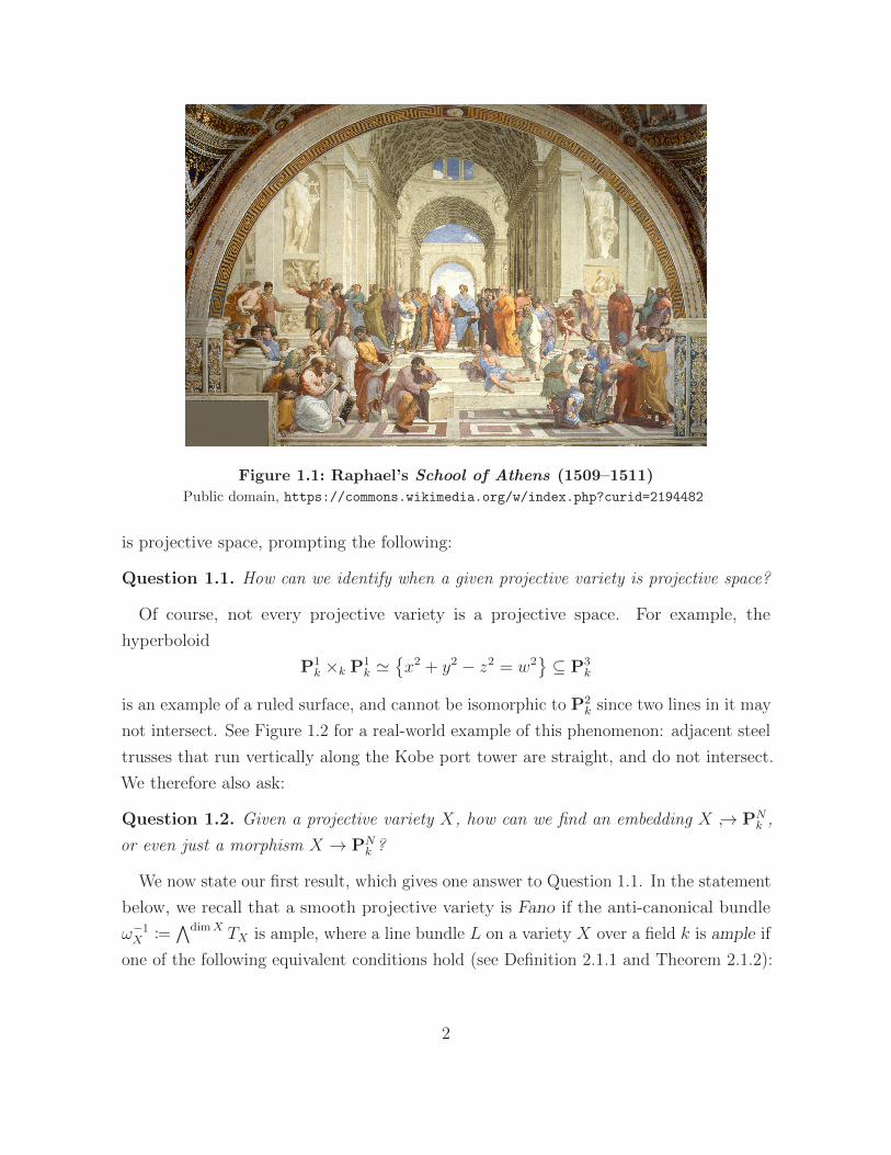
Figure 1.1: Raphael’s School of Athens (1509–1511)

Public domain, https://commons.wikimedia.org/w/index.php?curid=2194482

is projective space, prompting the following:

Question 1.1. How can we identify when a given projective variety is projective space?

Of course, not every projective variety is a projective space. For example, the

hyperboloid

P1k ×k P1

k 'x2 + y2 − z2 = w2

⊆ P3

k

is an example of a ruled surface, and cannot be isomorphic to P2k since two lines in it may

not intersect. See Figure 1.2 for a real-world example of this phenomenon: adjacent steel

trusses that run vertically along the Kobe port tower are straight, and do not intersect.

We therefore also ask:

Question 1.2. Given a projective variety X, how can we find an embedding X → PNk ,

or even just a morphism X → PNk ?

We now state our first result, which gives one answer to Question 1.1. In the statement

below, we recall that a smooth projective variety is Fano if the anti-canonical bundle

ω−1X :=

∧dimX TX is ample, where a line bundle L on a variety X over a field k is ample if

one of the following equivalent conditions hold (see Definition 2.1.1 and Theorem 2.1.2):

2

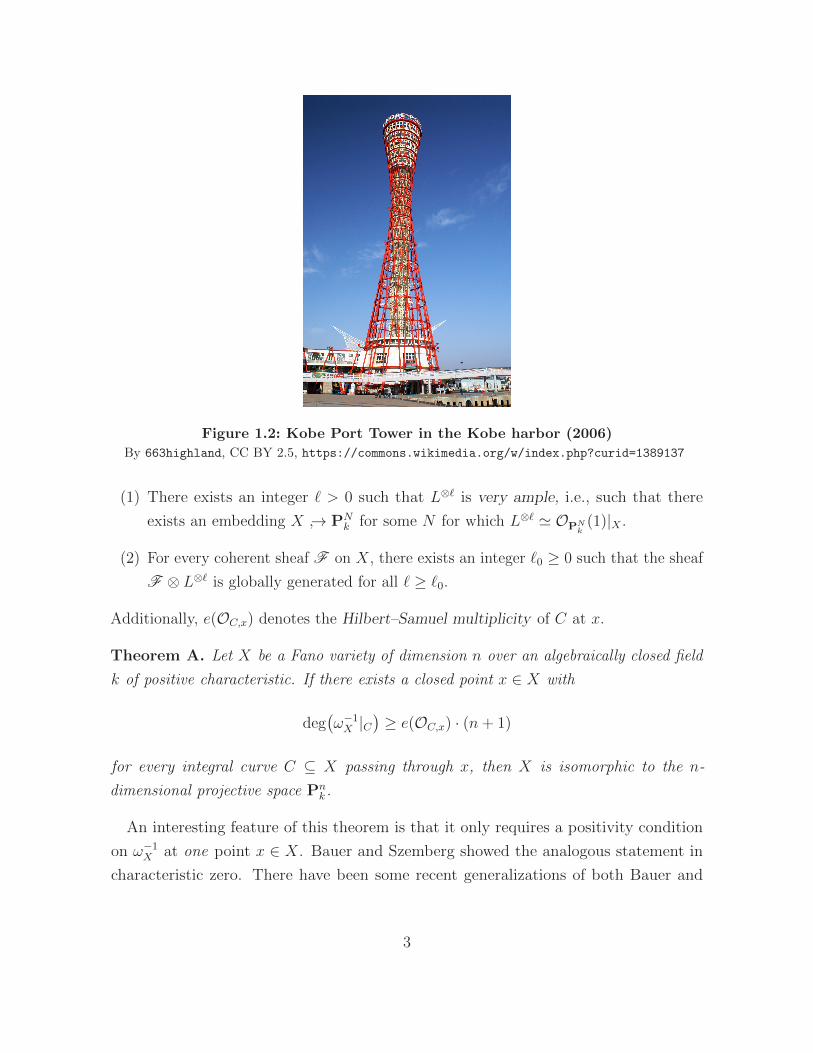
Figure 1.2: Kobe Port Tower in the Kobe harbor (2006)

By 663highland, CC BY 2.5, https://commons.wikimedia.org/w/index.php?curid=1389137

(1) There exists an integer ` > 0 such that L⊗` is very ample, i.e., such that there

exists an embedding X → PNk for some N for which L⊗` ' OPNk

(1)|X .

(2) For every coherent sheaf F on X, there exists an integer `0 ≥ 0 such that the sheaf

F ⊗ L⊗` is globally generated for all ` ≥ `0.

Additionally, e(OC,x) denotes the Hilbert–Samuel multiplicity of C at x.

Theorem A. Let X be a Fano variety of dimension n over an algebraically closed field

k of positive characteristic. If there exists a closed point x ∈ X with

deg(ω−1X |C

)≥ e(OC,x) · (n+ 1)

for every integral curve C ⊆ X passing through x, then X is isomorphic to the n-

dimensional projective space Pnk .

An interesting feature of this theorem is that it only requires a positivity condition

on ω−1X at one point x ∈ X. Bauer and Szemberg showed the analogous statement in

characteristic zero. There have been some recent generalizations of both Bauer and

3

Szemberg’s result and of Theorem A due to Liu and Zhuang; see Remark 3.2.3. There is

also an interesting connection between Theorem A and the Mori–Mukai conjecture (see

Conjecture 3.1.5), which states that if X is a Fano variety of dimension n such that the

anti-canonical bundle ω−1X satisfies deg(ω−1

X |C) ≥ n + 1 for all rational curves C ⊆ X,

then X is isomorphic to Pnk . Theorem A strengthens the positivity assumption on ω−1

X

to incorporate the multiplicity of the curves passing through x, but has the advantage

of not having to impose any generality conditions on the point x. See §3.1 for further

discussion.

Our next result is the main ingredient in proving Theorem A, and gives a partial

answer to Question 1.2. We motivate this result by first stating Fujita’s conjecture, a

proof of which would answer Question 1.2. Below, ωX :=∧dimX ΩX is the canonical

bundle on X.

Conjecture 1.3 [Fuj87, Conj.; Fuj88, no 1]. Let X be a smooth projective variety of

dimension n over an algebraically closed field k, and let L be an ample line bundle on X.

We then have the following:

(i) (Fujita’s freeness conjecture) ωX ⊗ L⊗` is globally generated for all ` ≥ n+ 1.

(ii) (Fujita’s very ampleness conjecture) ωX ⊗ L⊗` is very ample for all ` ≥ n+ 2.

The essence of Fujita’s conjecture is that an ample line bundle L can effectively and

uniformly be turned into a globally generated or very ample line bundle. Over the

complex numbers, Fujita’s freeness conjecture holds in dimensions ≤ 5 [Rei88; EL93a;

Kaw97; YZ], and Fujita’s very ampleness conjecture holds in dimensions ≤ 2 [Rei88]. On

the other hand, in arbitrary characteristic, much less is known. While the same proof as

over the complex numbers works for curves, only partial results are known for surfaces

[SB91; Ter99; DCF15], and in higher dimensions, we only know that Fujita’s conjecture

1.3 holds when L is additionally assumed to be globally generated [Smi97]. See §2.1 and

especially Table 2.1 for a summary of existing results.

We now describe our approach to Fujita’s conjecture 1.3, and state our second main

result. In 1992, Demailly introduced Seshadri constants to measure the local positivity of

line bundles with the hope that they could be used to prove cases of Fujita’s conjecture

[Dem92, §6]. These constants are defined as follows. Let L be an ample line bundle on a

4

projective variety X over an algebraically closed field, and consider a closed point x ∈ X.

The Seshadri constant of L at x is

ε(L;x) := supt ∈ R≥0

∣∣ µ∗L(−tE) is ample, (1.2)

where µ : X → X is the blowup of X at x with exceptional divisor E. The connection

between Seshadri constants and Fujita’s conjecture 1.3 is given by the following result,

which says that if the Seshadri constant ε(L;x) is sufficiently large, then ωX ⊗ L has

many global sections. This is the main ingredient in the proof of Theorem A.

Theorem B. Let X be a smooth projective variety of dimension n over an algebraically

closed field k of characteristic p > 0, and let L be an ample line bundle on X. Let x ∈ Xbe a closed point, and consider an integer ` ≥ 0. If ε(L;x) > n+ `, then ωX⊗L separates

`-jets at x, i.e., the restriction morphism

H0(X,ωX ⊗ L) −→ H0(X,ωX ⊗ L⊗OX/m`+1x )

is surjective, where mx ⊆ OX is the ideal defining x.

In particular, then, to show Fujita’s freeness conjecture 1.3(i), it would suffice to show

that ε(L;x) > nn+1

for every point x ∈ X, where n = dimX. Theorem B was proved

over the complex numbers by Demailly; see Proposition 2.2.6. In positive characteristic,

the special case when ` = 0 is due to Mustata and Schwede [MS14, Thm. 3.1]. Our

contribution is that the same result holds for all ` ≥ 0 in positive characteristic.

Remark 1.4. Theorem B holds more generally for line bundles that are not necessarily

ample, and for certain singular varieties over arbitrary fields; see Theorem 7.3.1. This

version of Theorem B for singular varieties is new even over the complex numbers, and

we do not know of a proof of this more general result that does not reduce to the

positive characteristic case. Moreover, by combining Theorem 7.3.1 with lower bounds

on Seshadri constants due to Ein, Kuchle, and Lazarsfeld (Theorem 2.2.11), we obtain

generic results toward Fujita’s conjecture 1.3 for singular varieties; see Corollary 2.2.13

and Remark 2.2.14.

The main difficulty in proving Theorem B is that Kodaira-type vanishing theorems

can fail in positive characteristic. Recall that if X is a smooth projective variety over

5

the complex numbers, and L is an ample line bundle on X, then the Kodaira vanishing

theorem states that

H i(X,ωX ⊗ L) = 0

for every i > 0. This vanishing theorem was a critical ingredient in Demailly’s proof

of Theorem B over the complex numbers. In positive characteristic, however, the

Kodaira vanishing theorem is often false, as was first discovered by Raynaud [Ray78] (see

Example 2.4.4). We note that the strategy behind known cases of Fujita’s conjecture 1.3

is to construct global sections of ωX ⊗ L⊗` inductively by using versions of the Kodaira

vanishing theorem to lift sections from smaller dimensional subvarieties. It has therefore

been thought that the failure of vanishing theorems may be the greatest obstacle to

making progress on Fujita’s conjecture 1.3 in positive characteristic.

In order to replace vanishing theorems, we build on the theory of so-called “Frobenius

techniques.” A key insight in positive characteristic algebraic geometry is that while

vanishing theorems are false, there is one major advantage to working in positive

characteristic: every variety X has an interesting endomorphism, called the Frobenius

morphism. This endomorphism F : X → X is defined as the identity map on points, and

the p-power map

OX(U) F∗OX(U)

f fp

on functions over every open set U ⊆ X, where p is the characteristic of the ground field

k. Even if one is only interested in algebraic geometry over the complex numbers, some

results necessitate reducing to the case when the ground field is of positive characteristic

and then using the Frobenius morphism. For example, this “reduction modulo p”

technique is used in one proof of the Ax–Grothendieck theorem, which says that an

injective polynomial endomorphism Cn → Cn is bijective [Ax68, Thm. C; EGAIV3,

Prop. 10.4.11], and in Mori’s bend and break technique, which is used to find rational

curves on varieties [Mor79, §2]. The latter in particular is a fundamental technique in

modern birational geometry, but there is no known direct proof of Mori’s theorems over

the complex numbers.

In its current form, Frobenius techniques were developed simultaneously in commutative

algebra (see, e.g., [HR76; HH90]) and in representation theory (see, e.g., [MR85; RR85]).

Particularly important is the theory of tight closure developed by Hochster and Huneke,

6

which was used by Smith to show special cases of Fujita’s conjecture [Smi97; Smi00a].

The Frobenius techniques used in proving Theorem B can be used to give progress

toward Fujita’s conjecture 1.3. As mentioned above, Theorem B implies that to show

Fujita’s freeness conjecture 1.3(i), it would suffice to show that ε(L;x) > nn+1

for every

point x ∈ X, where n = dimX. Unfortunately, Miranda showed that the Seshadri

constant ε(L;x) can get arbitrarily small at special points x ∈ X; see Example 2.2.9.

Nevertheless, we show that the dimension n in the statement of Theorem B can be

replaced by a smaller number, called the log canonical threshold, over which one has

more control. See Definition 4.8.6 for a precise definition of the log canonical threshold.

This invariant is associated to the data of the variety X together with a formal Q-

linear combination ∆ of codimension one subvarieties of X, and measures how bad the

singularities of X and ∆ are. We also mention that ε(‖H‖;x) below denotes the moving

Seshadri constant of H at x, which is a version of the Seshadri constant defined above in

(1.2) for line bundles that are not necessarily ample; see Definition 7.1.1.

Theorem C. Let (X,∆) be an effective log pair such that X is a projective normal

variety over a field k of characteristic zero, and such that KX +∆ is Q-Cartier. Consider

a k-rational point x ∈ X such that (X,∆) is klt, and suppose that D is a Cartier divisor

on X such that H = D − (KX + ∆) satisfies

ε(‖H‖;x

)> lctx

((X,∆);mx

).

Then, OX(D) has a global section not vanishing at x.

While we have stated Theorem C over a field of characteristic zero, our proof uses

reduction modulo p and Frobenius techniques to reduce to a similar result in positive

characteristic (Theorem 8.1.1).

Using Theorem C, we then show the following version of a theorem of Angehrn and

Siu [AS95, Thm. 0.1]. Our statement is modeled after that in [Kol97, Thm. 5.8]. Below,

volX|Z(H) denotes the restricted volume, which measures how many global sections

OZ(mH|Z) has on Z that are restrictions of global sections of OX(mH) on X as m→∞;

see Definition 4.6.13.

Theorem D. Let (X,∆) be an effective log pair, where X is a normal projective variety

over an algebraically closed field k of characteristic zero, ∆ is a Q-Weil divisor, and

7

KX + ∆ is Q-Cartier. Let x ∈ X be a closed point such that (X,∆) is klt at x, and let

D be a Cartier divisor on X such that setting H := D − (KX + ∆), there exist positive

numbers c(m) with the following properties:

(i) For every positive dimensional variety Z ⊆ X containing x, we have

volX|Z(H) > c(dimZ)dimZ .

(ii) The numbers c(m) satisfy the inequality

dimX∑

m=1

m

c(m)≤ 1.

Then, OX(D) has a global section not vanishing at x.

A version of this result for smooth complex projective varieties appears in [ELM+09,

Thm. 2.20]. As a consequence, we recover the following result, which gives positive

evidence toward Fujita’s freeness conjecture 1.3(i).

Corollary 1.5 (cf. [AS95, Cor. 0.2]). Let X be a smooth projective variety of dimension

n over an algebraically closed field of characteristic zero, and let L be an ample line bundle

on X. Then, the line bundle ωX ⊗ L⊗` is globally generated for all ` ≥ 12n(n+ 1) + 1.

This corollary is obtained from Theorem D by setting c(m) =(n+1

2

)for every m. Since

we prove Corollary 1.5 without the use of Kodaira-type vanishing theorems, Theorem D

and Corollary 1.5 support the validity of the following:

Principle 1.6. The failure of Kodaira-type vanishing theorems is not the main obstacle

to proving Fujita’s conjecture 1.3 over fields of positive characteristic.

Instead, the difficulty is in constructing certain boundary divisors that are very singular

at a point, but have mild singularities elsewhere; cf. Theorem 8.2.1.

Finally, we mention one intermediate result used in the proofs of Theorems C and D,

which is of independent interest. This statement characterizes ampleness in terms of

asymptotic growth of higher cohomology groups. It is well known that if X is a projective

variety of dimension n > 0, then hi(X,OX(mL)) := dimkHi(X,OX(mL)) = O(mn) for

8

every Cartier divisor L; see [Laz04a, Ex. 1.2.20]. It is therefore natural to ask when

cohomology groups have submaximal growth. The following result says that ample

Cartier divisors L are characterized by having submaximal growth of higher cohomology

groups for small perturbations of L.

Theorem E. Let X be a projective variety of dimension n > 0 over a field k. Let L be

an R-Cartier divisor on X. Then, L is ample if and only if there exists a very ample

Cartier divisor A on X and a real number ε > 0 such that

hi(X,L− tA) := lim supm→∞

hi(X,OX

(dm(L− tA)e

))

mn/n!= 0

for all i > 0 and for all t ∈ [0, ε).

Here, the hi(X,−) are the asymptotic higher cohomological functions introduced

by Kuronya [Kur06]; see §4.6.3. Theorem E was first proved by de Fernex, Kuronya,

and Lazarsfeld over the complex numbers [dFKL07, Thm. 4.1]. We note that one can

have hi(X,L) = 0 for all i > 0 without L being ample, or even pseudoeffective; see

Example 6.1.1.

1.1. Outline

This thesis is divided into two parts, followed by two appendices. The first part consists

of Chapters 2 and 3, and is more introductory in nature. In Chapter 2, we give more

motivation and many examples illustrating the questions we are studying in this thesis.

After highlighting some difficulties in positive characteristic, we prove Theorem B. We

then devote Chapter 3 to proving our characterization of projective space (Theorem A).

The second part of this thesis consists of the remaining chapters. In Chapters 4 and 5,

we review some preliminary material that will be used in the rest of the thesis. Since

almost all of this material is not new, we recommend the reader to skip ahead to the

results they are interested in, and to refer back to these preliminary chapters as necessary.

We then focus on proving Theorem 7.3.1, which is a generalization of Theorem B for

singular varieties, and on proving Theorems C and D. To do so, we prove Theorem E in

Chapter 6, which is used when we study moving Seshadri constants in Chapter 7. This

9

latter chapter is also where we prove Theorem 7.3.1. Finally, we prove Theorems C and

D in Chapter 8.

The two appendices are devoted to some technical aspects of the theory of F -

singularities for rings and schemes whose Frobenius endomorphisms are not necessarily

finite. Appendix A reviews the definitions of and relationships between different classes

of F -singularities, and Appendix B develops a scheme-theoretic version of the gamma

construction of Hochster–Huneke, which we use throughout the thesis to reduce to the

case when the ground field k satisfies [k : kp] <∞, where char k = p > 0.

1.2. Notation and conventions

We mostly follow the notation and conventions of [Har77] for generalities in algebraic

geometry, of [Laz04a; Laz04b] for positivity of divisors, line bundles, and vector bundles,

and of [Har66] for Grothendieck duality theory. See also the List of Symbols. A notable

exception is that we do not assume anything a priori about the ground field that we work

over, and in particular, the ground field may not be algebraically closed or even perfect.

All rings are commutative with identity. A variety is a reduced and irreducible scheme

that is separated and of finite type over a field k. A complete scheme is a scheme

that is proper over a field k. Intersection products (LdimV · V ) are defined using Euler

characteristics, following Kleiman; see [Kle05, App. B].

10

Chapter 2

Motivation and examples

In this chapter, we motivate the questions posed in the introduction with some more

background and examples. The new material is a slight modification of Kollar’s example

2.1.6 to work in arbitrary characteristic, and the proof of Theorem B; see §2.4.1. A

different proof of Theorem B originally appeared in [Mur18, §3].

2.1. Fujita’s conjecture

To motivate Fujita’s conjectural answer to Question 1.2, we give some background. First,

we recall the following definition.

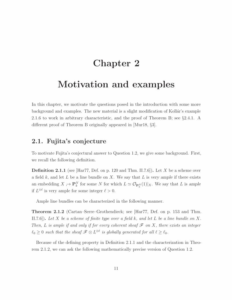
Definition 2.1.1 (see [Har77, Def. on p. 120 and Thm. II.7.6]). Let X be a scheme over

a field k, and let L be a line bundle on X. We say that L is very ample if there exists

an embedding X → PNk for some N for which L ' OPNk

(1)|X . We say that L is ample

if L⊗` is very ample for some integer ` > 0.

Ample line bundles can be characterized in the following manner.

Theorem 2.1.2 (Cartan–Serre–Grothendieck; see [Har77, Def. on p. 153 and Thm.

II.7.6]). Let X be a scheme of finite type over a field k, and let L be a line bundle on X.

Then, L is ample if and only if for every coherent sheaf F on X, there exists an integer

`0 ≥ 0 such that the sheaf F ⊗ L⊗` is globally generated for all ` ≥ `0.

Because of the defining property in Definition 2.1.1 and the characterization in Theo-

rem 2.1.2, we can ask the following mathematically precise version of Question 1.2.

11

Question 2.1.3. Let L be an ample line bundle on a projective variety X. What power

of L is very ample or globally generated?

The best thing we could hope for is that the power needed in Question 2.1.3 depends

on some invariants of X. For curves, we can give a very explicit answer to Question 2.1.3.

We use the language of divisors instead of line bundles below to simplify notation.

Example 2.1.4 (Curves I; see [Har77, Cor. IV.3.2]). Let X be a smooth curve over

an algebraically closed field k, i.e., a projective variety of dimension 1 over k. Let D

be a divisor on X. We claim that the complete linear system |D| is basepoint-free if

degD ≥ 2g, and is very ample if degD ≥ 2g + 1, where g is the genus of X. Recall that

by [Har77, Prop. IV.3.1], the complete linear system |D| is basepoint-free if and only if

h0(X,OX(D − P )

)= h0

(X,OX(D)

)− 1

for every closed point P ∈ X, and is very ample if and only if

h0(X,OX(D − P −Q)

)= h0

(X,OX(D)

)− 2

for every pair of closed points P,Q ∈ X. We will verify these properties below.

Suppose degD ≥ 2g (resp. degD ≥ 2g+1). By Serre duality, we have h1(X,OX(D)) =

0, and h1(X,OX(D − P −Q)) = 0 for every closed point P ∈ X (resp. h1(X,OX(D −P −Q)) = 0 for every two closed points P,Q ∈ X). We therefore have

h0(X,OX(D − P )

)= deg(D − P ) + 1− g= degD − 1 + 1− g = h0

(X,OX(D)

)− 1

h0(X,OX(D − P −Q)

)= deg(D − P −Q) + 1− g= degD − 2 + 1− g = h0

(X,OX(D)

)− 2

in each case by the Riemann–Roch theorem [Har77, Thm. IV.1.3]. As a result, we see

that if L is an ample divisor on X, the complete linear system |`L| is basepoint-free for

all ` ≥ 2g, and is very ample for all ` ≥ 2g + 1, where g is the genus of X.

We can answer Question 2.1.3 for abelian varieties as well.

12

F1

F2

∆

B

X = E × E

3 : 1

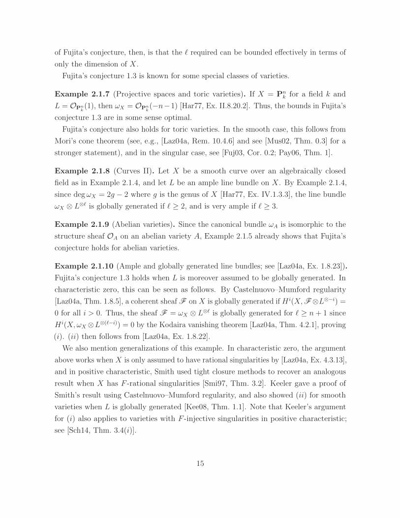
fY

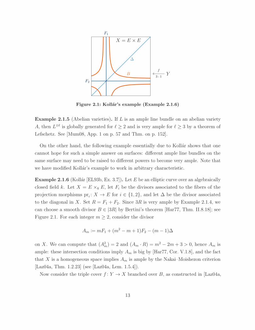
Figure 2.1: Kollar’s example (Example 2.1.6)

Example 2.1.5 (Abelian varieties). If L is an ample line bundle on an abelian variety

A, then L⊗` is globally generated for ` ≥ 2 and is very ample for ` ≥ 3 by a theorem of

Lefschetz. See [Mum08, App. 1 on p. 57 and Thm. on p. 152].

On the other hand, the following example essentially due to Kollar shows that one

cannot hope for such a simple answer on surfaces: different ample line bundles on the

same surface may need to be raised to different powers to become very ample. Note that

we have modified Kollar’s example to work in arbitrary characteristic.

Example 2.1.6 (Kollar [EL93b, Ex. 3.7]). Let E be an elliptic curve over an algebraically

closed field k. Let X = E ×k E, let Fi be the divisors associated to the fibers of the

projection morphisms pri : X → E for i ∈ 1, 2, and let ∆ be the divisor associated

to the diagonal in X. Set R = F1 + F2. Since 3R is very ample by Example 2.1.4, we

can choose a smooth divisor B ∈ |3R| by Bertini’s theorem [Har77, Thm. II.8.18]; see

Figure 2.1. For each integer m ≥ 2, consider the divisor

Am := mF1 + (m2 −m+ 1)F2 − (m− 1)∆

on X. We can compute that (A2m) = 2 and (Am · R) = m2 − 2m+ 3 > 0, hence Am is

ample: these intersection conditions imply Am is big by [Har77, Cor. V.1.8], and the fact

that X is a homogeneous space implies Am is ample by the Nakai–Moishezon criterion

[Laz04a, Thm. 1.2.23] (see [Laz04a, Lem. 1.5.4]).

Now consider the triple cover f : Y → X branched over B, as constructed in [Laz04a,

13

Prop. 4.1.6]. For every m ≥ 2, the divisors Dm := f ∗Am are ample by [Laz04a, Prop.

1.2.13], but we claim that mDm is not ample. It suffices to show that the pullback

homomorphism

f ∗ : H0(X,OX(mAm)

)−→ H0

(Y,OY (mDm)

)(2.1)

is an isomorphism, since if this were the case, then the morphism

Y|mDm|−−−−→ P

(H0(Y,OY (mDm)

))

would factor through the 3 : 1 morphism f . To show that (2.1) is an isomorphism, we

first note that

f∗(OY (mDm)

)' f∗OY ⊗OX(mAm)

' OX(mAm)⊕OX(mAm −R)⊕OX(mAm − 2R)(2.2)

by the projection formula and by the construction of Y (see [Laz04a, Rem. 4.1.7]). On

global sections, the inclusion H0(X,OX(mAm)) → H0(X, f∗(OY (mDm))) induced by

the isomorphism (2.2) can be identified with the pullback homomorphism (2.1) by the

construction of Y . On the other hand, since (mAm − R)2 < 0 and (mAm − 2R)2 < 0,

we have that H0(X,OX(mAm − R)) = H0(X,OX(mAm − 2R)) = 0 by [Laz04a, Lem.

1.5.4]. Thus, (2.1) is an isomorphism.

To get bounds only in terms of the dimension of X, Mukai suggested that the correct

bundles to look at are adjoint line bundles, i.e., line bundles of the form ωX ⊗ L, where

ωX is the canonical bundle on X. In this direction, Fujita conjectured the following:

Conjecture 1.3 [Fuj87, Conj.; Fuj88, no 1]. Let X be a smooth projective variety of

dimension n over an algebraically closed field, and let L be an ample line bundle on X.

We then have the following:

(i) (Fujita’s freeness conjecture) ωX ⊗ L⊗` is globally generated for all ` ≥ n+ 1.

(ii) (Fujita’s very ampleness conjecture) ωX ⊗ L⊗` is very ample for all ` ≥ n+ 2.

Note that both properties hold for some `: (i) holds for some ` by Theorem 2.1.2, and

for (ii), it suffices to note that if ωX ⊗L⊗`1 is globally generated and L⊗`2 is very ample,

then their tensor product ωX ⊗L⊗(`1+`2) is very ample [EGAII, Prop. 4.4.8]. The essence

14

of Fujita’s conjecture, then, is that the ` required can be bounded effectively in terms of

only the dimension of X.

Fujita’s conjecture 1.3 is known for some special classes of varieties.

Example 2.1.7 (Projective spaces and toric varieties). If X = Pnk for a field k and

L = OPnk(1), then ωX = OPnk

(−n−1) [Har77, Ex. II.8.20.2]. Thus, the bounds in Fujita’s

conjecture 1.3 are in some sense optimal.

Fujita’s conjecture also holds for toric varieties. In the smooth case, this follows from

Mori’s cone theorem (see, e.g., [Laz04a, Rem. 10.4.6] and see [Mus02, Thm. 0.3] for a

stronger statement), and in the singular case, see [Fuj03, Cor. 0.2; Pay06, Thm. 1].

Example 2.1.8 (Curves II). Let X be a smooth curve over an algebraically closed

field as in Example 2.1.4, and let L be an ample line bundle on X. By Example 2.1.4,

since degωX = 2g − 2 where g is the genus of X [Har77, Ex. IV.1.3.3], the line bundle

ωX ⊗ L⊗` is globally generated if ` ≥ 2, and is very ample if ` ≥ 3.

Example 2.1.9 (Abelian varieties). Since the canonical bundle ωA is isomorphic to the

structure sheaf OA on an abelian variety A, Example 2.1.5 already shows that Fujita’s

conjecture holds for abelian varieties.

Example 2.1.10 (Ample and globally generated line bundles; see [Laz04a, Ex. 1.8.23]).

Fujita’s conjecture 1.3 holds when L is moreover assumed to be globally generated. In

characteristic zero, this can be seen as follows. By Castelnuovo–Mumford regularity

[Laz04a, Thm. 1.8.5], a coherent sheaf F on X is globally generated if H i(X,F⊗L⊗−i) =

0 for all i > 0. Thus, the sheaf F = ωX ⊗ L⊗` is globally generated for ` ≥ n+ 1 since

H i(X,ωX⊗L⊗(`−i)) = 0 by the Kodaira vanishing theorem [Laz04a, Thm. 4.2.1], proving

(i). (ii) then follows from [Laz04a, Ex. 1.8.22].

We also mention generalizations of this example. In characteristic zero, the argument

above works when X is only assumed to have rational singularities by [Laz04a, Ex. 4.3.13],

and in positive characteristic, Smith used tight closure methods to recover an analogous

result when X has F -rational singularities [Smi97, Thm. 3.2]. Keeler gave a proof of

Smith’s result using Castelnuovo–Mumford regularity, and also showed (ii) for smooth

varieties when L is globally generated [Kee08, Thm. 1.1]. Note that Keeler’s argument

for (i) also applies to varieties with F -injective singularities in positive characteristic;

see [Sch14, Thm. 3.4(i)].

15

Dimension Result (over C) Method

1 Classical [Har77, Cor. IV.3.2(a)] Riemann–Roch

2 Reider [Rei88, Thm. 1(i)] Bogomolov instability

3 Ein–Lazarsfeld [EL93a, Cor. 2*]Cohomological method of

Kawamata–Reid–Shokurov4 Kawamata [Kaw97, Thm. 4.1]

5 Ye–Zhu [YZ, Main Thm.]

Table 2.1: Known cases of Fujita’s freeness conjecture over the complex numbers

For general smooth complex projective varieties, Fujita’s freeness conjecture 1.3(i)

holds in dimensions n ≤ 5 (see Table 2.1) while Fujita’s very ampleness conjecture 1.3(ii)

is only known in dimensions n ≤ 2 [Rei88, Thm. 1(ii)]. In positive characteristic, the

usual statement of Fujita’s conjecture holds for surfaces that are neither quasi-elliptic

nor of general type [SB91, Cor. 8], and weaker bounds are known for quasi-elliptic and

general type surfaces [Ter99, Thm.; DCF15, Thm. 1.4].

In arbitrary dimension, one of the best results toward Fujita’s conjecture so far is the

following result due to Angehrn and Siu, which they proved using analytic methods.

Theorem 2.1.11 [AS95, Cor. 0.2]. Let X be a smooth complex projective variety of

dimension n, and let L be an ample line bundle on X. Then, the line bundle ωX ⊗ L⊗`is globally generated for all ` ≥ 1

2n(n+ 1) + 1.

Kollar later gave an algebraic proof of Theorem 2.1.11, which also applies to klt

pairs [Kol97, Thm. 5.8]. Improved lower bounds for ` have also been obtained by

Helmke [Hel97, Thm. 1.3; Hel99, Thm. 4.4] and Heier [Hei02, Thm. 1.4]. Note that

Theorem 2.1.11 is a special case of Theorem D, which we will prove later in this thesis,

since we can set c(m) =(n+1

2

)for all m; see Corollary 1.5.

2.2. Seshadri constants

To study Fujita’s conjecture 1.3, Demailly introduced Seshadri constants, which measure

the local positivity of nef divisors. Recall that an R-Cartier divisor D is nef if (D ·C) ≥ 0

for every curve C ⊆ X. See Definition 4.2.1 for the definition of an R-Cartier divisor.

16

H

C

x

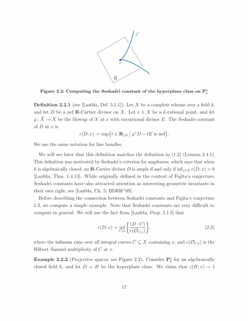
Figure 2.2: Computing the Seshadri constant of the hyperplane class on Pnk

Definition 2.2.1 (see [Laz04a, Def. 5.1.1]). Let X be a complete scheme over a field k,

and let D be a nef R-Cartier divisor on X. Let x ∈ X be a k-rational point, and let

µ : X → X be the blowup of X at x with exceptional divisor E. The Seshadri constant

of D at x is

ε(D;x) := supt ∈ R≥0

∣∣ µ∗D − tE is nef.

We use the same notation for line bundles.

We will see later that this definition matches the definition in (1.2) (Lemma 2.4.1).

This definition was motivated by Seshadri’s criterion for ampleness, which says that when

k is algebraically closed, an R-Cartier divisor D is ample if and only if infx∈X ε(D;x) > 0

[Laz04a, Thm. 1.4.13]. While originally defined in the context of Fujita’s conjecture,

Seshadri constants have also attracted attention as interesting geometric invariants in

their own right; see [Laz04a, Ch. 5; BDRH+09].

Before describing the connection between Seshadri constants and Fujita’s conjecture

1.3, we compute a simple example. Note that Seshadri constants are very difficult to

compute in general. We will use the fact from [Laz04a, Prop. 5.1.5] that

ε(D;x) = infC3x

(D · C)

e(OC,x)

, (2.3)

where the infimum runs over all integral curves C ⊆ X containing x, and e(OC,x) is the

Hilbert–Samuel multiplicity of C at x.

Example 2.2.2 (Projective spaces; see Figure 2.2). Consider Pnk for an algebraically

closed field k, and let D = H be the hyperplane class. We claim that ε(H;x) = 1

17

for every closed point x ∈ Pnk . By Bezout’s theorem [Har77, Thm. I.7.7], we have

(H ·C) ≥ e(OC,x) for every such curve C 3 x, hence ε(H;x) ≥ 1 by (2.3). The inequality

ε(H;x) ≤ 1 also holds by considering the case when C is a line containing x.

Example 2.2.2 can be generalized as follows.

Example 2.2.3 (Ample and globally generated line bundles; see [Laz04a, Ex. 5.1.18]).

We claim that if D is an ample and free Cartier divisor, then ε(D;x) ≥ 1. Let C 3 x be

a curve; it suffices to show that (D · C) ≥ e(OC,x). Since the complete linear system |D|is basepoint-free, there exists a divisor H ∈ |D| such that H does not contain C. We

then see that

(D · C) = deg(D|C) ≥ `(OD|C ,x) ≥ e(OC,x),

where the first inequality follows from definition (see [GW10, Def. 15.29]) and the second

inequality is a consequence of [Mat89, Thm. 14.10].

Demailly’s original motivation for defining Seshadri constants seems to have been its

potential application to Fujita’s conjecture 1.3. Before we state the result realizing this

connection, we make the following definition.

Definition 2.2.4. Let X be a scheme, and let F be a coherent sheaf on X. Fix a

closed point x ∈ X, and denote by mx ⊆ OX the ideal sheaf defining x. For every integer

` ≥ −1, we say that F separates `-jets at x if the restriction morphism

H0(X,F ) −→ H0(X,F/m`+1x F ) (2.4)

is surjective. We denote by s(F ;x) the largest integer ` ≥ −1 such that F separates `-jets

at x. If F = OX(D) for a Cartier divisor D, then we denote s(D;x) := s(OX(D);x).

Remark 2.2.5. The convention that s(F ;x) = −1 if F does not separate `-jets for

every ` ≥ 0 is from [FMa, Def. 6.1]. This differs from the convention s(F ;x) = −∞,

which is used in [Dem92, p. 96] and [Mur18, Def. 2.1], and the convention s(F ;x) = 0,

which is used in [ELM+09, p. 646]. Our convention is chosen to make a variant of the

Seshadri constant defined using jet separation (Definition 7.2.4) detect augmented base

loci (Lemma 7.2.6), while distinguishing whether or not F has any non-vanishing global

sections.

18

We now prove the following result due to Demailly, which connects Seshadri constants

to separation of jets.

Proposition 2.2.6 [Dem92, Prop. 6.8(a)]. Let X be a smooth projective variety of

dimension n over an algebraically closed field of characteristic zero, and let L be a big

and nef divisor on X. Let x ∈ X be a closed point, and consider an integer ` ≥ 0. If

ε(L;x) > n+ `, then ωX ⊗OX(L) separates `-jets at x.

Proof. Consider the short exact sequence

0 −→ m`+1x · ωX ⊗OX(L) −→ ωX ⊗OX(L) −→ ωX ⊗OX(L)⊗OX/m`+1

x −→ 0.

By the associated long exact sequence on sheaf cohomology, to show the surjectivity of

the restriction morphism (2.4), it suffices to show that

H1(X,m`+1

x · ωX ⊗OX(L))' H1

(X, µ∗

(ωX ⊗OX(L)

)(−(`+ 1)E

))

' H1(X, ωX ⊗OX

(µ∗L− (n+ `)E

))= 0,

where µ : X → X is the blowup of X at x. Here, the first isomorphism follows from

the Leray spectral sequence and the quasi-isomorphism m`+1x ' Rµ∗OX(−(` + 1)E)

[Laz04a, Lem. 4.3.16], and the second isomorphism follows from how the canonical

bundle transforms under a blowup with a smooth center [Har77, Exer. II.8.5(b)]. The

vanishing of the last group follows from the Kawamata–Viehweg vanishing theorem

[Laz04a, Thm. 4.3.1] since µ∗L− (n+ `)E is nef by the assumption ε(L;x) > n+ `, and

is big because by [Laz04a, Prop. 5.1.9], we have

(µ∗L− (n+ `)E

)n= (Ln)− (n+ `)n ≥

(ε(L;x)

)n − (n+ `)n > 0.

Demailly showed that a similar technique can be used to deduce separation of points

from the existence of lower bounds on Seshadri constants, and in particular, that if

infx∈X ε(L;x) > 2n where n = dimX, then ωX ⊗OX(L) is very ample [Dem92, Prop.

6.8(b)]. Because of these results, Demailly asked:

Question 2.2.7 [Dem92, Quest. 6.9]. Given a smooth projective variety X over an

19

algebraically closed field and an ample divisor L on X, does there exist a lower bound for

ε(L) := infx∈X

ε(L;x) ?

If such a lower bound were to exist, could we compute this lower bound explicitly in terms

of geometric invariants of X?

Remark 2.2.8. We note that the divisors constructed in Kollar’s example 2.1.6 do not

give a counterexample to Question 2.2.7. In the notation of Example 2.1.6, the divisor

2Am is free on X by Example 2.1.5. The pullback 2Dm = f ∗(2Am) is therefore ample

and free, hence ε(2Dm;x) ≥ 1 for every point x ∈ Y . By the homogeneity of Seshadri

constants [Laz04a, Ex. 5.1.4], we have ε(Dm;x) ≥ 1/2.

A very optimistic answer to Question 2.2.7 would be that ε(L) > nn+1

where n = dimX,

since if this were the case, Proposition 2.2.6 would then imply Fujita’s freeness conjecture

1.3(i). The following example of Miranda, however, shows that ε(L) can become

arbitrarily small, even on smooth surfaces.

Example 2.2.9 (Miranda [EL93b, Ex. 3.1]). Let δ > 0 be arbitrary. We will construct

a smooth projective surface X over an algebraically closed field k such that ε(L;x) < δ

for an ample divisor L on X and a closed point x ∈ X.

Choose an integer m ≥ 1 such that 1m< δ, and let Γ ⊆ P2

k be an integral curve of

degree d ≥ 3 and multiplicity m at a closed point ξ ∈ P2k. Let Γ′ ⊆ P2

k be a general

curve of degree d, which by generality we may assume is integral and intersects Γ in d2

reduced points. We moreover claim that for general Γ′, every curve in the pencil |W |spanned by Γ and Γ′ is irreducible. Note that such a pencil is a one-dimensional linear

system, while the codimension of the space of reducible curves in |dH| is

(d+ 2

2

)− max

1≤i≤d−1

(i+ 2

2

)+

(d− i+ 2

2

)+ 1

≥ (d+ 1)(d+ 2)

2−(d

2+ 1

)(d

2+ 2

)+ 1 =

d2

4≥ 2,

by the assumption d ≥ 3. Thus, for general Γ′, the pencil |W | does not contain any

reducible curves.

We now consider the blowup X → P2k along Γ ∩ Γ′ (see Figure 2.3). Since we have

20

Γ′

Γ

ξ

P2k

E

x

C C ′

X

P1k

π

blowup

Γ ∩ Γ′

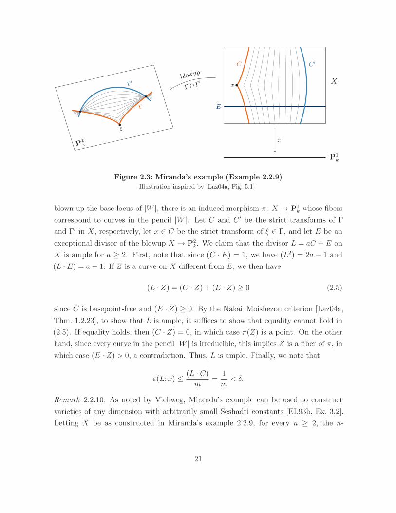
Figure 2.3: Miranda’s example (Example 2.2.9)

Illustration inspired by [Laz04a, Fig. 5.1]

blown up the base locus of |W |, there is an induced morphism π : X → P1k whose fibers

correspond to curves in the pencil |W |. Let C and C ′ be the strict transforms of Γ

and Γ′ in X, respectively, let x ∈ C be the strict transform of ξ ∈ Γ, and let E be an

exceptional divisor of the blowup X → P2k. We claim that the divisor L = aC + E on

X is ample for a ≥ 2. First, note that since (C · E) = 1, we have (L2) = 2a − 1 and

(L · E) = a− 1. If Z is a curve on X different from E, we then have

(L · Z) = (C · Z) + (E · Z) ≥ 0 (2.5)

since C is basepoint-free and (E · Z) ≥ 0. By the Nakai–Moishezon criterion [Laz04a,

Thm. 1.2.23], to show that L is ample, it suffices to show that equality cannot hold in

(2.5). If equality holds, then (C · Z) = 0, in which case π(Z) is a point. On the other

hand, since every curve in the pencil |W | is irreducible, this implies Z is a fiber of π, in

which case (E · Z) > 0, a contradiction. Thus, L is ample. Finally, we note that

ε(L;x) ≤ (L · C)

m=

1

m< δ.

Remark 2.2.10. As noted by Viehweg, Miranda’s example can be used to construct

varieties of any dimension with arbitrarily small Seshadri constants [EL93b, Ex. 3.2].

Letting X be as constructed in Miranda’s example 2.2.9, for every n ≥ 2, the n-

21

dimensional smooth projective variety X ×k Pn−2k satisfies

ε(p∗1L⊗ p∗2O(1); (x, z)

)≤ ε(L;x)

for every z ∈ Pn−2k by considering the curve C ×k z, where p1, p2 are the first and

second projection morphisms, respectively.

Bauer has also shown that Miranda’s example is not as exceptional as it might appear:

suitable blowups of any surface with Picard number one have arbitrarily small Seshadri

constants [Bau99, Prop. 3.3].

Despite Miranda’s example, Ein, Kuchle, and Lazarsfeld were able to prove that at

very general points on complex projective varieties, lower bounds for ε(L;x) do exist.

Theorem 2.2.11 [EKL95, Thm. 1]. Let X be a complex projective variety of dimension

n, and let L be a big and nef divisor on X. Then, for all closed points x ∈ X outside of

a countable union of proper closed subvarieties in X, we have

ε(L;x) ≥ 1

n.

Moreover, for every δ > 0, the locus

x ∈ X

∣∣∣∣ ε(L;x) >1

n+ δ

contains a Zariski-open dense set in X(C).

When L is ample and X is smooth of dimension n ≤ 3, the lower bound in Theo-

rem 2.2.11 can be improved to ε(L;x) ≥ 1/(n− 1) [EL93b, Thm.; CN14, Thm. 1.2]. The

case n = 2 supports the following strengthening of Theorem 2.2.11.

Conjecture 2.2.12 [EKL95, p. 194]. Let X be a projective variety over an algebraically

closed field, and let L be a big and nef divisor on X. Then, for all closed points x ∈ Xoutside of a countable union of proper closed subvarieties of X, we have ε(L;x) ≥ 1.

By combining Proposition 2.2.6 and Theorem 2.2.11, we obtain the following:

Corollary 2.2.13. Let X be a smooth complex projective variety of dimension n, and

let L be a big and nef divisor on X. Then, the bundle ωX ⊗ L⊗m separates `-jets at all

22

general points x ∈ X for all m ≥ n(n+ `) + 1. In particular, we have

h0(X,ωX ⊗ L⊗m) ≥(n+ `

n

)

for all m ≥ n(n+ `) + 1.

Remark 2.2.14. By replacing Proposition 2.2.6 with Theorem 7.3.1, we see that Corol-

lary 2.2.13 holds for X with singularities of at worst dense F -injective type. See Defini-

tion 5.6.7 for the definition of this class of singularities. In particular, Corollary 2.2.13

holds for X with at worst rational singularities by Figure 5.1.

2.3. A relative Fujita-type conjecture

We also mention the following relative version of Fujita’s conjecture. Inspired by

Kollar and Viehweg’s work on weak positivity, which partially answers an analogue of

Question 1.2 for families of varieties, Popa and Schnell proposed the following:

Conjecture 2.3.1 [PS14, Conj. 1.3]. Let f : Y → X be a morphism of smooth complex

projective varieties, where X is of dimension n, and let L be an ample line bundle on X.

Then, for every k ≥ 1, the sheaf f∗ω⊗kY ⊗ L⊗m is globally generated for all m ≥ k(n+ 1).

Note that if f is the identity morphism X → X, then Conjecture 2.3.1 is identical

to Fujita’s freeness conjecture 1.3(i). Popa and Schnell proved Conjecture 2.3.1 when

dimX = 1 [PS14, Prop. 2.11], or when L is additionally assumed to be globally generated

[PS14, Thm. 1.4]. This latter result was shown using Castelnuovo–Mumford regularity

in a similar fashion to Example 2.1.10, with Ambro and Fujino’s Kollar-type vanishing

theorem replacing the Kodaira vanishing theorem in the proof.

In joint work with Yajnaseni Dutta, we proved the following effective global generation

result in the spirit of Conjecture 2.3.1, which we later extended to higher-order jets in

joint work with Mihai Fulger. Note that the case when (Y,∆) is klt and k = 1 is due to

de Cataldo [dC98, Thm. 2.2].

Theorem 2.3.2 [DM19, Thm. A; FMa, Cor. 8.2]. Let f : Y → X be a surjective

morphism of complex projective varieties, where X is of dimension n. Let (Y,∆) be a log

canonical pair and let L be a big and nef line bundle on X. Consider a Cartier divisor

23

P on Y such that P ∼R k(KY + ∆) for some integer k ≥ 1. Then, the sheaf

f∗OY (P )⊗ L⊗m

separates `-jets at all general points x ∈ X for all m ≥ k(n(n+ `) + 1).

The proof of Theorem 2.3.2 is a relativization of the argument in Proposition 2.2.6,

and uses the lower bound on Seshadri constants in Theorem 2.2.11. A generic global

generation result in this direction was first obtained by Dutta for klt Q-pairs (Y,∆)

[Dut, Thm. A]. Using analytic techniques, Deng and Iwai later obtained improvements

of Dutta’s original result for klt pairs with better lower bounds, under the additional

assumption that X is smooth and L is ample [Den, Thm. C; Iwa, Thm. 1.5]. In [DM19,

Thm. B], we proved algebraic versions of Deng’s and Iwai’s results as a consequence of a

new weak positivity result for pairs [DM19, Thms. E and F]. Note, however, that only

our methods in [DM19; FMa] apply to log canonical pairs.

Remark 2.3.3. In positive characteristic, there is an example of a curve fibration over P1k

which gives a counterexample both to Popa and Schnell’s relative Fujita-type conjecture

2.3.1, and to the analogue of Theorem 2.3.2 in positive characteristic. The example is

based on a construction due to Moret-Bailly [MB81]; see [SZ, Prop. 4.11].

2.4. Difficulties in positive characteristic

While most of the questions, conjectures, and examples seen so far have been stated

over fields of arbitrary characteristic, the majority of the results stated, in particular

on Fujita’s conjecture (Table 2.1 and Theorem 2.1.11) and lower bounds on Seshadri

constants (Theorem 2.2.11), are only known over fields of characteristic zero. The most

problematic situation is when the ground field k is an imperfect field of characteristic

p > 0, in which case there are at least three major difficulties. First, since k is of

characteristic p > 0,

(I) Resolutions of singularities are not known to exist (see [Hau10]), and

(II) Kodaira-type vanishing theorems are false [Ray78] (see §2.4.2).

A common workaround for the lack of resolutions is to use de Jong’s theory of alterations

[dJ96]. The lack of vanishing theorems is harder to circumvent, however, since over the

24

complex numbers, vanishing theorems are a fundamental ingredient used to construct

global sections of line bundles. A useful workaround is to exploit the Frobenius morphism

F : X → X and its Grothendieck trace F∗ω•X → ω•X ; see [PST17; Pat18]. For imperfect

fields, however, this approach runs into another problem:

(III) Applications of Frobenius techniques in algebraic geometry usually require the

ground field k to be F -finite, i.e., satisfy [k : kp] <∞.

The last issue arises since Grothendieck duality cannot be applied to the Frobenius if it

is not finite. Working around this last issue is the focus of Appendix B.

2.4.1. Proof of Theorem B

To illustrate how Frobenius techniques can be used in practice, we prove the following

positive characteristic version of Proposition 2.2.6.

Theorem B. Let X be a smooth projective variety of dimension n over an algebraically

closed field k of characteristic p > 0, and let L be an ample line bundle on X. Let x ∈ Xbe a closed point, and consider an integer ` ≥ 0. If ε(L;x) > n+ `, then ωX⊗L separates

`-jets at x.

The case ` = 0 is due to Mustata and Schwede [MS14, Thm. 3.1]. The case for

arbitrary ` ≥ 0 first appeared in [Mur18, Thm. A]. These proofs used a positive-

characteristic version of Seshadri constants called Frobenius–Seshadri constants ε`F (L;x);

see Remark 7.3.4. Note that we will later prove a generalization of Theorem B; see

Theorem 7.3.1.

We give a new proof of Theorem B, which is an adaptation of the proof in [PST17,

Exer. 6.3], which proves the case when ` = 0. As in the proof of [MS14, Thm. 3.1], the

main ingredient in the proof is the Grothendieck trace

TrX : F∗ωX −→ ωX

associated to the (absolute) Frobenius morphism F : X → X. Recall that the Frobenius

morphism is defined as the identity map on points, and the p-power map

OX(U) F∗OX(U)

f fp

25

on functions over every open set U ⊆ X. This map TrX is a morphism of OX-modules,

which can be obtained by applying Grothendieck duality for finite flat morphisms to the

(absolute) Frobenius morphism F : X → X; see §4.4. Note that F is finite since k is

F -finite (see Example 5.3.2), and is flat by Kunz’s theorem [Kun69, Thm. 2.1] since X

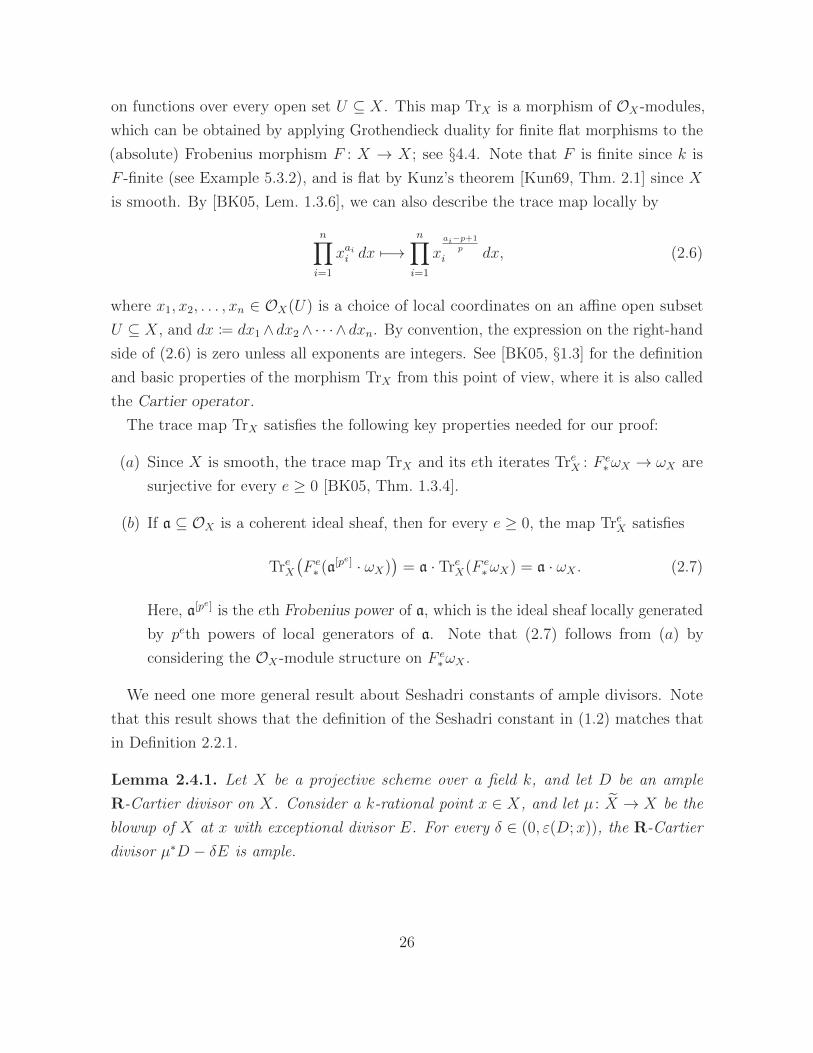
is smooth. By [BK05, Lem. 1.3.6], we can also describe the trace map locally by

n∏

i=1

xaii dx 7−→n∏

i=1

xai−p+1

p

i dx, (2.6)

where x1, x2, . . . , xn ∈ OX(U) is a choice of local coordinates on an affine open subset

U ⊆ X, and dx := dx1∧dx2∧ · · ·∧dxn. By convention, the expression on the right-hand

side of (2.6) is zero unless all exponents are integers. See [BK05, §1.3] for the definition

and basic properties of the morphism TrX from this point of view, where it is also called

the Cartier operator.

The trace map TrX satisfies the following key properties needed for our proof:

(a) Since X is smooth, the trace map TrX and its eth iterates TreX : F e∗ωX → ωX are

surjective for every e ≥ 0 [BK05, Thm. 1.3.4].

(b) If a ⊆ OX is a coherent ideal sheaf, then for every e ≥ 0, the map TreX satisfies

TreX(F e∗ (a

[pe] · ωX))

= a · TreX(F e∗ωX) = a · ωX . (2.7)

Here, a[pe] is the eth Frobenius power of a, which is the ideal sheaf locally generated

by peth powers of local generators of a. Note that (2.7) follows from (a) by

considering the OX-module structure on F e∗ωX .

We need one more general result about Seshadri constants of ample divisors. Note

that this result shows that the definition of the Seshadri constant in (1.2) matches that

in Definition 2.2.1.

Lemma 2.4.1. Let X be a projective scheme over a field k, and let D be an ample

R-Cartier divisor on X. Consider a k-rational point x ∈ X, and let µ : X → X be the

blowup of X at x with exceptional divisor E. For every δ ∈ (0, ε(D;x)), the R-Cartier

divisor µ∗D − δE is ample.

26

Proof. Let V ⊆ X be a subvariety. If V 6⊆ E, then V is the strict transform of a

subvariety V0 ⊆ X, and

((µ∗D − δE

)dimV · V)

=(DdimV · V0

)− δ e(OV0,x) > 0

by the assumption ε(D;x) > δ and [Laz04a, Prop. 5.1.9]. Otherwise, if V ⊆ E, then

((µ∗D − δE

)dimV · V)

=((−δE|E

)dimV · V)> 0

since OE(−E|E) ' OPn−1(1) is very ample. Thus, the divisor µ∗D − δE is ample by the

Nakai–Moishezon criterion [Laz04a, Thm. 1.2.23].

We can now prove Theorem B.

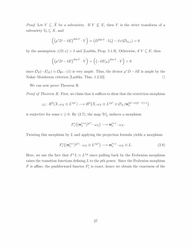
Proof of Theorem B. First, we claim that it suffices to show that the restriction morphism

ϕe : H0(X,ωX ⊗ L⊗pe

) −→ H0(X,ωX ⊗ L⊗p

e ⊗OX/m`pe+n(pe−1)+1x

)

is surjective for some e ≥ 0. By (2.7), the map TreX induces a morphism

F e∗((m`+1

x )[pe] · ωX)−→ m`+1

x · ωX .

Twisting this morphism by L and applying the projection formula yields a morphism

F e∗((m`+1

x )[pe] · ωX ⊗ L⊗pe) −→ m`+1

x · ωX ⊗ L. (2.8)

Here, we use the fact that F ∗L ' L⊗p since pulling back by the Frobenius morphism

raises the transition functions defining L to the pth power. Since the Frobenius morphism

F is affine, the pushforward functor F e∗ is exact, hence we obtain the exactness of the

27

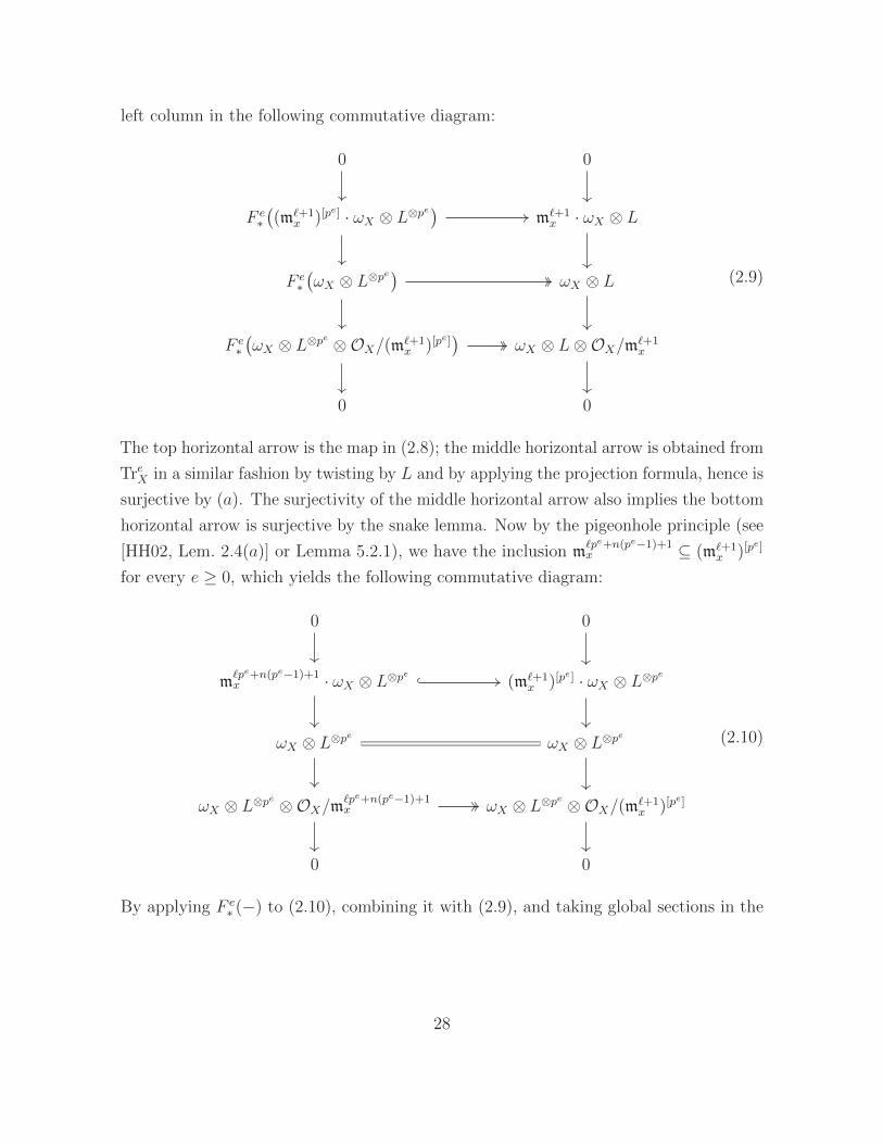
left column in the following commutative diagram:

0 0

F e∗((m`+1

x )[pe] · ωX ⊗ L⊗pe)

m`+1x · ωX ⊗ L

F e∗(ωX ⊗ L⊗pe

)ωX ⊗ L

F e∗(ωX ⊗ L⊗pe ⊗OX/(m`+1

x )[pe])

ωX ⊗ L⊗OX/m`+1x

0 0

(2.9)

The top horizontal arrow is the map in (2.8); the middle horizontal arrow is obtained from

TreX in a similar fashion by twisting by L and by applying the projection formula, hence is

surjective by (a). The surjectivity of the middle horizontal arrow also implies the bottom

horizontal arrow is surjective by the snake lemma. Now by the pigeonhole principle (see

[HH02, Lem. 2.4(a)] or Lemma 5.2.1), we have the inclusion m`pe+n(pe−1)+1x ⊆ (m`+1

x )[pe]

for every e ≥ 0, which yields the following commutative diagram:

0 0

m`pe+n(pe−1)+1x · ωX ⊗ L⊗pe (m`+1

x )[pe] · ωX ⊗ L⊗pe

ωX ⊗ L⊗pe ωX ⊗ L⊗pe

ωX ⊗ L⊗pe ⊗OX/m`pe+n(pe−1)+1x ωX ⊗ L⊗pe ⊗OX/(m`+1

x )[pe]

0 0

(2.10)

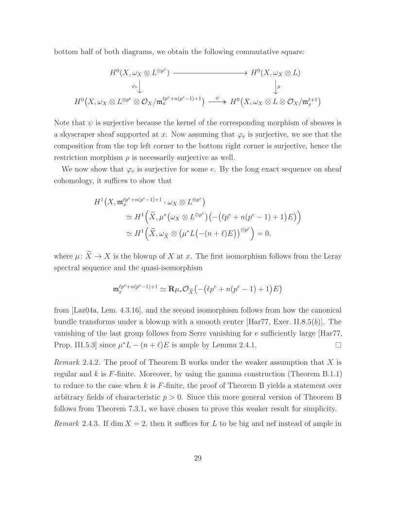
By applying F e∗ (−) to (2.10), combining it with (2.9), and taking global sections in the

28

bottom half of both diagrams, we obtain the following commutative square:

H0(X,ωX ⊗ L⊗pe) H0(X,ωX ⊗ L)

H0(X,ωX ⊗ L⊗pe ⊗OX/m`pe+n(pe−1)+1

x

)H0(X,ωX ⊗ L⊗OX/m`+1

x

)ϕe ρ

ψ

Note that ψ is surjective because the kernel of the corresponding morphism of sheaves is

a skyscraper sheaf supported at x. Now assuming that ϕe is surjective, we see that the

composition from the top left corner to the bottom right corner is surjective, hence the

restriction morphism ρ is necessarily surjective as well.

We now show that ϕe is surjective for some e. By the long exact sequence on sheaf

cohomology, it suffices to show that

H1(X,m`pe+n(pe−1)+1

x · ωX ⊗ L⊗pe)

' H1(X, µ∗

(ωX ⊗ L⊗p

e)(−(`pe + n(pe − 1) + 1

)E))

' H1(X, ωX ⊗

(µ∗L

(−(n+ `)E

))⊗pe)= 0,

where µ : X → X is the blowup of X at x. The first isomorphism follows from the Leray

spectral sequence and the quasi-isomorphism

m`pe+n(pe−1)+1x ' Rµ∗OX

(−(`pe + n(pe − 1) + 1

)E)

from [Laz04a, Lem. 4.3.16], and the second isomorphism follows from how the canonical

bundle transforms under a blowup with a smooth center [Har77, Exer. II.8.5(b)]. The

vanishing of the last group follows from Serre vanishing for e sufficiently large [Har77,

Prop. III.5.3] since µ∗L− (n+ `)E is ample by Lemma 2.4.1.

Remark 2.4.2. The proof of Theorem B works under the weaker assumption that X is

regular and k is F -finite. Moreover, by using the gamma construction (Theorem B.1.1)

to reduce to the case when k is F -finite, the proof of Theorem B yields a statement over

arbitrary fields of characteristic p > 0. Since this more general version of Theorem B

follows from Theorem 7.3.1, we have chosen to prove this weaker result for simplicity.

Remark 2.4.3. If dimX = 2, then it suffices for L to be big and nef instead of ample in

29

Theorem B. To prove this, it suffices to replace Serre vanishing with a vanishing theorem

of Szpiro [Szp79, Prop. 2.1] and Lewin-Menegaux [LM81, Prop. 2], which asserts that for

a big and nef divisor L on a smooth projective surface X, we have

H1(X,OX(−mL)

)= 0

for m sufficiently large. Fujita has shown that a similar vanishing theorem also holds for

higher-dimensional projective varieties that are only assumed to be normal [Fuj83, Thm.

7.5], although the positivity condition on L is stronger. Fujita’s theorem cannot be used

to prove Theorem B in higher dimensions for big and nef divisors L, however, since the

required vanishing Hn−1(X,OX(−mL)) = 0 does not hold in general, even as m→∞;

see Example 2.4.5.

2.4.2. Raynaud’s counterexample to Kodaira vanishing

To illustrate what goes wrong in positive characteristic, we give a version of Raynaud’s

original example showing that Kodaira vanishing is false in positive characteristic, with

some changes in presentation following Mukai [Muk79; Muk13]. See also [Tak10; Zhe17].

Note that Mukai also constructs versions of Raynaud’s example in higher dimensions.

Example 2.4.4 (Raynaud [Ray78; Muk79; Muk13]). Let k be an algebraically closed

field of characteristic p > 0. The construction proceeds in four steps.

Step 1. Construction of a smooth projective curve C over k and a Cartier divisor D on

C such that the morphism

F ∗ : H1(C,OC(−D)

)−→ H1

(C,OC(−pD)

)(2.11)

induced by the Frobenius morphism is not injective.

Let h > 0 be an integer, let P be a polynomial of degree h in one variable over k, and

consider the plane curve

C =P (xp)− x = yph−1

⊆ P2

k

of degree ph, where P2k has variables x, y, z, and P (xp) − x = yph−1 is the equation

defining C on the open set z 6= 0. Note that C has exactly one point ∞ along

30

z = 0. By the Jacobian criterion [Har77, Exer. I.5.8], since the homogeneous Jacobian

(−zph−1, yph−2z, xzph−2 − yph−1) associated to C has full rank along C, we see that C

is smooth.

We claim that the morphism (2.11) is not injective for the divisor D = h(ph− 3) · ∞.

By [Tan72, Lem. 12], since the kernel of the morphism in (2.11) can be described by

ker(F ∗) 'df ∈ ΩK(C)

∣∣ f ∈ K(C) such that (df) ≥ pD,

it suffices to construct a rational function f ∈ K(C) satisfying (df) ≥ pD. Here, (df) is

the divisor of zeroes and poles of the differential form df . Consider the rational function

y ∈ K(C). By the relation −dx = −yph−2dy on C r ∞, we see that ΩC is generated

by dy over C r ∞, hence dy has no poles or zeroes away from ∞. Since by [Har77,

Ex. V.1.5.1], we have

deg ΩC = 2g(C)− 2 = ph(ph− 3), (2.12)

we obtain (dy) = ph(ph− 3) · ∞ = pD, as desired. We note that C is an example of a

Tango curve.

Step 2. Construction of a projective bundle π : P(E)→ C with two distinguished divisors

F and G arising from sections of P(E) and of P(E(p)).

By identifying the sheaf cohomology groups in (2.11) with Ext1 groups [Har77, Prop.

III.6.3], we obtain a short exact sequence

0 −→ OC −→ E −→ OC(D) −→ 0 (2.13)

such that after pulling back via the Frobenius morphism F : C → C on C, the resulting

short exact sequence

0 −→ OC −→ E(p) −→ OC(pD) −→ 0 (2.14)

splits. The projective bundles of one-dimensional quotients P(E) and P(E(p)) associated

31

C

P(E) P(E(p))

F F ′

G G′

ϕ

f

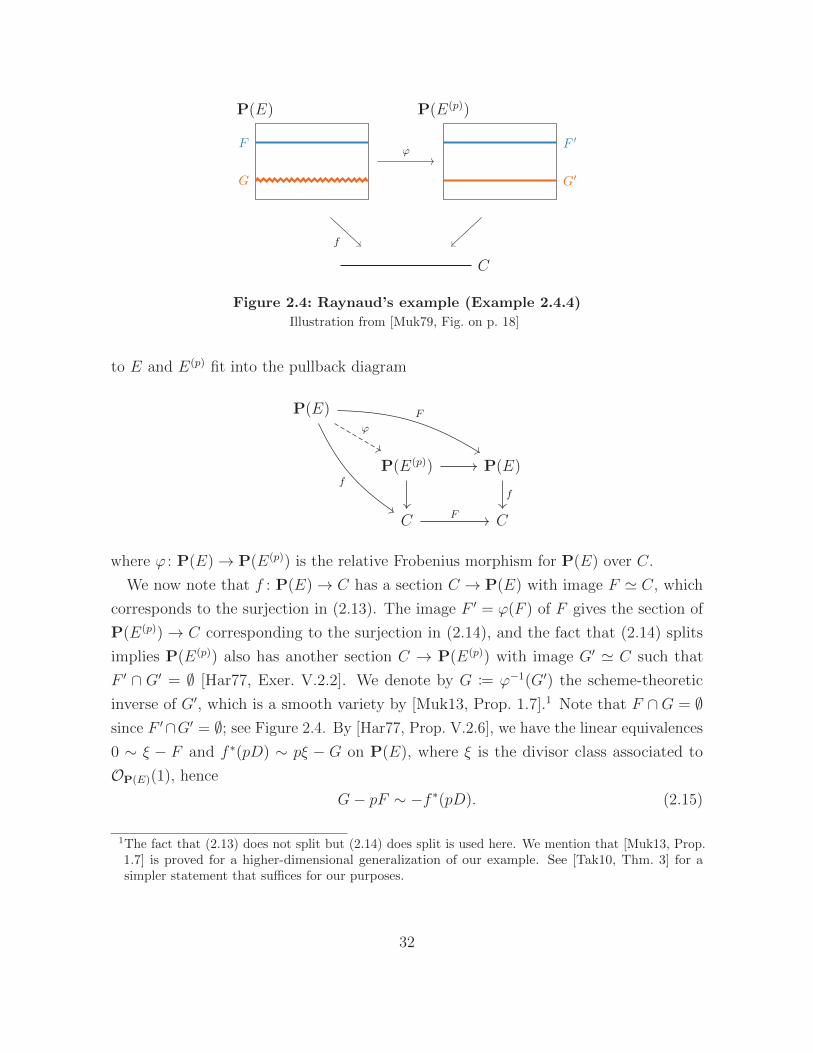
Figure 2.4: Raynaud’s example (Example 2.4.4)

Illustration from [Muk79, Fig. on p. 18]

to E and E(p) fit into the pullback diagram

P(E)

P(E(p)) P(E)

C C

ϕ

F

ff

F

where ϕ : P(E)→ P(E(p)) is the relative Frobenius morphism for P(E) over C.

We now note that f : P(E)→ C has a section C → P(E) with image F ' C, which

corresponds to the surjection in (2.13). The image F ′ = ϕ(F ) of F gives the section of

P(E(p))→ C corresponding to the surjection in (2.14), and the fact that (2.14) splits

implies P(E(p)) also has another section C → P(E(p)) with image G′ ' C such that

F ′ ∩ G′ = ∅ [Har77, Exer. V.2.2]. We denote by G := ϕ−1(G′) the scheme-theoretic

inverse of G′, which is a smooth variety by [Muk13, Prop. 1.7].1 Note that F ∩G = ∅since F ′∩G′ = ∅; see Figure 2.4. By [Har77, Prop. V.2.6], we have the linear equivalences

0 ∼ ξ − F and f ∗(pD) ∼ pξ − G on P(E), where ξ is the divisor class associated to

OP(E)(1), hence

G− pF ∼ −f ∗(pD). (2.15)

1The fact that (2.13) does not split but (2.14) does split is used here. We mention that [Muk13, Prop.1.7] is proved for a higher-dimensional generalization of our example. See [Tak10, Thm. 3] for asimpler statement that suffices for our purposes.

32

Step 3. Construction of a cyclic cover π : X → P(E) where X is a smooth surface and

a suitable ample divisor D on X.

Let r ≥ 2 be an integer such that r | p+ 1 and r | h(ph− 3) for some choice of integer

h > 0 in Step 1. For example, if p 6= 2 then we can set r = 2 for arbitrary h > 0; if

p = 2, then we can set r = 3 for h > 0 such that 3 | h. By adding (p+ 1)F to (2.15), we

have G+ F ∼ (p+ 1)F − f ∗(pD) ∼ rM , where

M :=p+ 1

rF − f ∗

(ph(ph− 3)

r· ∞),

since D = h(ph− 3) · ∞. We can therefore construct a degree r cyclic cover

X := SpecP(E)

(OP(E) ⊕OP(E)(−M)⊕ · · · ⊕ OP(E)

(−(r − 1)M

)) π−→ P(E)

branched along G + F , which is smooth by the fact that both P(E) and G + F are

smooth [Laz04a, Prop. 4.1.6]. We then set

D = F + (f π)∗(h(ph− 3)

r· ∞),

where F = π−1(F )red is the inverse image of F with reduced scheme structure. To show

that D is ample, we first note that F +f ∗(h(ph−3) ·∞) is ample by the Nakai–Moishezon

criterion [Laz04a, Thm. 1.2.23] since it intersects both the section F and the fibers of the

ruled surface f : P(E)→ C positively. The pullback rD ∼ π∗(rF ) + π∗f ∗(h(ph− 3) ·∞)

is therefore also ample by [Laz04a, Prop. 4.1.6], hence D is ample. We note that X is an

example of a Raynaud surface.

Step 4. Proof that H1(X,OX(−D)) 6= 0.

First, we note that

H1(X,OX(−D)

)' H1

(P(E), π∗OX(−D)

)

' H1

(P(E),OP(E)(−F )⊕

r−1⊕

i=1

OP(E)(−iM)

).

The first isomorphism holds by the fact that π is finite. The second isomorphism holds

by properties of cyclic covers; see [Zhe16, Prop. 6.3.4] for a proof using local coordinates,

33

or see [Zhe17, Prop. 3.3] for a shorter proof. Now consider the Leray spectral sequence

Ep,q2 = Hp

(C,Rqf∗

(OP(E)(−F )⊕

r−1⊕

i=1

OP(E)(−iM)

))

⇒ Hp+q

(P(E),OP(E)(−F )⊕

r−1⊕

i=1

OP(E)(−iM)

) (2.16)

which already degenerates on the E2 page. We have that E1,02 = 0, since the pushforward

f∗

(OP(E)(−F )⊕

r−1⊕

i=1

OP(E)(−iM)

)

' f∗OP(E)(−1)⊕r−1⊕

i=1

f∗OP(E)

(−i(p+ 1)

r

)⊗OC

(iph(ph− 3)

r· ∞)

is zero by the fact that f∗OP(E)(−n) = 0 for n > 0. Thus, the Leray spectral sequence

(2.16) implies that

H1(X,OX(−D)

)' H0

(C,R1f∗

(OP(E)(−F )⊕

r−1⊕

i=1

OP(E)(−iM)

)). (2.17)

Since R1f∗(OP(E)(−F )) ' R1f∗(OP(E)(−1)) = 0, we will consider the summands con-

taining OP(E)(−iM). By [Har77, Exer. II.8.4(c)], we have

R1f∗

(OP(E)

(−i(p+ 1)

r

))'(f∗OP(E)

(i(p+ 1)− 2r

r

))∨'(Sym

i(p+1)−2rr E

)∨,

hence the projection formula implies

R1f∗(OP(E)(−iM)

)'(Sym

i(p+1)−2rr E

)∨ ⊗OC(iph(ph− 3)

r· ∞).

The short exact sequence (2.13) implies that there is a surjection Symi(p+1)−2r

r E

OC( i(p+1)−2r

rD), hence there is an injection

OC(

(2r − i)h(ph− 3)

r· ∞)−→ R1f∗

(OP(E)(−iM)

).

34

We therefore have

H0

(C,OC

((2r − i)h(ph− 3)

2· ∞))

−→ H0(C,R1f∗

(OP(E)(−iM)

)),

where the left-hand side is nonzero as long as 2r − i ≥ 0. By the assumption r ≥ 2, the

left-hand side is nonzero for i = 1, hence (2.17) implies H1(X,OX(−D)) 6= 0.

As noted by Fujita, Raynaud’s example 2.4.4 also gives counterexamples to the

vanishing theorem in Remark 2.4.3 for smooth projective varieties of dimension 3.

Example 2.4.5 [Fuj83, (7.10)]. Let X and D be as constructed in Example 2.4.4, and

consider the P1-bundle

Y := P(OX(D)⊕OX

) π−→ X

over X. Note that OY (1) is big and nef by [Laz04a, Lems. 2.3.2(iii) and 2.3.2(iv)]. We

claim that H2(Y,OY (−m)) 6= 0 for all m ≥ 2. We have

H2(Y,OY (−m)

)∨ ' H1(Y, ωY ⊗OY (m)

)

' H1(Y,OY (m− 2)⊗ π∗

(ωX ⊗OX(D)

))

by Serre duality [Har77, Cor. 7.7] and by [Har77, Exer. II.8.4(b)], respectively. By the

projection formula, we therefore have

H2(Y,OY (−m)

)∨ ' H1(X, Symm−2

(OX(D)⊕OX

)⊗ ωX ⊗OX(D)

).

The right-hand side contains H1(X,ωX ⊗ OX(D)) ' H1(X,OX(−D))∨ as a direct

summand for all m ≥ 2. Since H1(X,OX(−D)) 6= 0 by the construction in Example 2.4.4,

we see that H2(Y,OY (−m)) 6= 0 for all m ≥ 2.

35

Chapter 3

Characterizations of

projective space

In this chapter, we describe how Seshadri constants can be used to study the following:

Question 1.1. How can we identify when a given projective variety is projective space?

Recall that a smooth projective variety X of dimension n is Fano if its anti-canonical

bundle ω−1X :=

∧n TX is ample. In this chapter, we prove the following characterization

of projective space amongst Fano varieties using Seshadri constants. Note that the lower

bound deg(ω−1X |C) ≥ e(OC,x) · (n+ 1) below is equivalent to ε(ω−1

X ;x) ≥ n+ 1; see the

statement of Theorem A*.

Theorem A. Let X be a Fano variety of dimension n over an algebraically closed field

k of positive characteristic. If there exists a closed point x ∈ X with

deg(ω−1X |C

)≥ e(OC,x) · (n+ 1)

for every integral curve C ⊆ X passing through x, then X is isomorphic to the n-

dimensional projective space Pnk .

This result is originally due to Bauer and Szemberg in characteristic zero [BS09, Thm.

1.7]. The material in this chapter is from [Mur18, §4].

36

3.1. Background

We start by motivating the statement of Theorem A. Our story begins with the following

observation about projective space.

Principle 3.1.1. The n-dimensional projective space Pnk over a field k has a “positive”

tangent bundle TX . For example, we have the following:

(1) TX is an ample vector bundle [Laz04b, Prop. 6.3.1(i)].

(2) There exists an ample line bundle H on Pnk such that

∧n TX ' H⊗(n+1).

(3)∧n TX = ω−1

X is ample (i.e., X is Fano) and deg(ω−1X |C) ≥ n + 1 for all integral

curves C ⊆ X.

Note that (2) and (3) hold since ω−1Pnk

= OPnk(n+ 1) [Har77, Ex. II.8.20.2]. We recall that

a vector bundle E on X is ample if OP(E)(1) is ample [Laz04b, Def. 6.1.1].

These properties seem very special, and lead us to ask the following more specific

version of Question 1.1.

Question 3.1.2. Let X be a smooth projective variety of dimension n over an alge-

braically closed field k. If X satisfies one of (1)–(3), is X isomorphic to Pnk?

Many results in this direction are known. The first result, due to Mori, is in some

sense the birthplace of modern birational geometry and the minimal model program.

Theorem 3.1.3 [Mor79, Thm. 8]. Let X be a smooth projective variety of dimension n

over an algebraically closed field k. If (1) holds, then X is isomorphic to Pnk .

The sufficiency of (1) was first conjectured by Frankel [Fra61, Conj.] in the analytic

context, and by Hartshorne [Har70, Prob. III.2.3] in the algebraic context. The idea

of Mori’s proof is to produce many copies of P1k inside X passing through a point

x0 ∈ X using bend and break techniques. Letting µ : X → X be the blowup of X at

x0, Mori shows that X has the structure of a P1k-bundle over Pn−1

k ; see Figure 3.1 for

an illustration. This P1k-bundle structure for X forces X ' Pn

k [Kol96, Lem. V.3.7.8].

An interesting feature of Mori’s bend and break techniques is that in characteristic zero,

Mori’s techniques require reducing modulo p and utilizing the Frobenius morphism. It is

unknown whether one can prove Theorem 3.1.3 directly, without reducing modulo p.

37

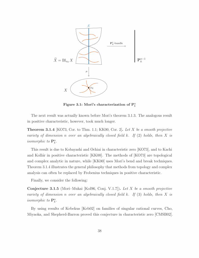
E

Pn−1k

µ

P1k-bundle

X = Blx0 X

Xx0

Figure 3.1: Mori’s characterization of Pnk

The next result was actually known before Mori’s theorem 3.1.3. The analogous result

in positive characteristic, however, took much longer.

Theorem 3.1.4 [KO73, Cor. to Thm. 1.1; KK00, Cor. 2]. Let X be a smooth projective

variety of dimension n over an algebraically closed field k. If (2) holds, then X is

isomorphic to Pnk .

This result is due to Kobayashi and Ochiai in characteristic zero [KO73], and to Kachi

and Kollar in positive characteristic [KK00]. The methods of [KO73] are topological

and complex analytic in nature, while [KK00] uses Mori’s bend and break techniques.

Theorem 3.1.4 illustrates the general philosophy that methods from topology and complex

analysis can often be replaced by Frobenius techniques in positive characteristic.

Finally, we consider the following:

Conjecture 3.1.5 (Mori–Mukai [Kol96, Conj. V.1.7]). Let X be a smooth projective

variety of dimension n over an algebraically closed field k. If (3) holds, then X is

isomorphic to Pnk .

By using results of Kebekus [Keb02] on families of singular rational curves, Cho,

Miyaoka, and Shepherd-Barron proved this conjecture in characteristic zero [CMSB02].

38

More precisely, they showed the following statement, which is stronger than the Mori–

Mukai conjecture 3.1.5 since Fano varieties are uniruled [Kol96, Cor. IV.1.15].

Theorem 3.1.6 [CMSB02, Cor. 0.4(11)]. Let X be a smooth projective variety of

dimension n over an algebraically closed field k of characteristic zero. If X is uniruled,

and the inequality

deg(ω−1X |C

)≥ n+ 1

holds for every rational curve C ⊆ X passing through a general closed point x0 ∈ X,

then X is isomorphic to Pnk .

Because of the assumption on the characteristic, we ask the following:

Question 3.1.7. Is the Mori–Mukai conjecture 3.1.5 true in positive characteristic?

In arbitrary characteristic, as far as we know the only result in this direction is the

following result due to Kachi and Kollar, which we state using the language of divisors.

Theorem 3.1.8 [KK00, Cor. 3]. Let X be a smooth projective variety of dimension n

over an algebraically closed field k. Suppose KX is not nef. If

(a) (−KX · C) ≥ n+ 1 for every rational curve C ⊆ X; and

(b) (−KX)n ≥ (n+ 1)n,

then X is isomorphic to Pnk .

The major issue in trying to mimic the proof in [CMSB02] is the use of deformation

theory and, more specifically, the use of generic smoothness in studying deformations of

curves. Note that generic smoothness is false in positive characteristic, since the absolute

Frobenius morphism F : X → X for a smooth variety X is nowhere smooth [Har77,

Ex. III.10.5.1]. One way to interpret Theorem A is that we avoid issues with generic

smoothness and deformation theory by building singularities into the statement of the

Mori–Mukai conjecture 3.1.5. The advantage of this modification is that Theorem A can

be interpreted in terms of Seshadri constants in the following manner.

Theorem A*. Let X be a Fano variety of dimension n over an algebraically closed field

k of positive characteristic. If there exists a closed point x ∈ X with ε(ω−1X ;x) ≥ (n+ 1),

then X is isomorphic to the n-dimensional projective space Pnk .

39

Note that the conditions in Theorem A and in Theorem A* are equivalent by (2.3).

Using this reinterpretation, we can show that Theorem A is a consequence of Theo-

rem 3.1.6 in characteristic zero, and a version of Theorem A assuming a slightly stronger

lower bound on ε(ω−1X ;x) at all points x ∈ X is a consequence of Theorem 3.1.8. The

statement in characteristic zero gives a different proof of [BS09, Thm. 1.7].

Proposition 3.1.9. Let X be a Fano variety of dimension n over an algebraically closed

field k. Suppose one of the following is satisfied:

(i) We have char k = 0 and ε(ω−1X ;x) > n holds for a single closed point x ∈ X; or

(ii) We have char k = p > 0 and ε(ω−1X ;x) ≥ n+ 1 holds for all closed points x ∈ X.

Then, X is isomorphic to Pnk .

Proof. For (i), we use Theorem 3.1.6. It suffices to verify the condition deg(ω−1X |C) > n.

First, the locus x ∈ X | ε(ω−1X ;x) > n contains a Zariski open set [EKL95, Lem.

1.4], hence we have ε(ω−1X ;x0) > n at a general point x0 ∈ X. By the alternative

characterization of Seshadri constants in terms of curves in (2.3), we have the chain of

inequalities

n < ε(ω−1X ;x0) ≤ deg(ω−1

X |C)

e(OC,x0)≤ deg(ω−1

X |C)

for any rational curve C containing x0.

For (ii), we use Theorem 3.1.8. The verification of condition (a) proceeds as in (i) by

applying (2.3) to a closed point x ∈ C contained in a given rational curve C ⊆ X. For

condition (b), we use the inequality ε(ω−1X ;x) ≤ n

√(−KX)n, which is [Laz04a, eq. 5.2].

The inequality ε(ω−1X ;x) ≥ n+ 1 then implies condition (b).

Given the similarity between the Mori–Mukai conjecture 3.1.5 and Theorem A, we ask

the following:

Question 3.1.10. Let X be a Fano variety of dimension n over an algebraically closed

field k. If the inequality

deg(ω−1X |C

)≥ n+ 1

holds for every curve C ⊆ X, then does there exist a closed point x ∈ X with

deg(ω−1X |C) ≥ e(OC,x) · (n+ 1)

40

for every curve C ⊆ X containing x?

The answer to this question is “yes” in characteristic zero by using Theorem 3.1.6,

since Theorem 3.1.6 implies X ' Pnk , and therefore the required positivity property

on ω−1X holds by Example 2.2.2. If one could answer Question 3.1.10 affirmatively

independently of Theorem 3.1.6, then [BS09, Thm. 1.7] would give an alternative proof

of the Mori–Mukai conjecture 3.1.5 in characteristic zero, and Theorem A would resolve

their conjecture in positive characteristic.

Finally, we mention another conjectural characterization of projective space that ties

in with our discussion in Chapter 1.

Remark 3.1.11. In Chapter 1, we noted that the cohomology ring of PnC is Z[h]/(hn+1);

see (1.1). Fujita conjectured that a smooth complex projective variety of dimension

n with this singular cohomology ring is isomorphic to PnC [Fuj80, Conj. Cn]. Fujita

himself proved this conjecture in dimensions n ≤ 5 [Fuj80, Thm. 1] (under the additional

assumption that X is Fano), and Libgober and Wood proved this conjecture in dimensions

n ≤ 6 [LW90, Thm. 1]. See also [Deb, Thm. 2]. It is unclear what the right formulation

of this conjecture would be in positive characteristic.

3.2. Proof of Theorem A

We now turn to the proof of Theorem A. The main technical tool is the notion of bundles

of principal parts, which are also known as jet bundles in the literature. See [LT95, §4]

or [EGAIV4, §16] for a detailed discussion.

Definition 3.2.1. Let X be a variety over an algebraically closed field k. Denote by p1

and p2 the projections

X ×k X

X X

p1 p2

Let I ⊂ OX×X be the ideal defining the diagonal, and let L be a line bundle on X. For

each integer ` ≥ 0, the `th bundle of principal parts associated to L is the sheaf

P`(L) := p1∗(p∗2L⊗OX×X/I `+1).

41

Note that P0(L) ' L, since the diagonal in X ×X is isomorphic to X.

We will use the following facts about these sheaves from [LT95, §4], under the

assumption that X is a smooth variety over an algebraically closed field.

(a) There exists a short exact sequence [LT95, no 4.2]

0 −→ Sym`(ΩX)⊗ L −→P`(L) −→P`−1(L) −→ 0, (3.1)

where ΩX denotes the cotangent bundle on X. By using induction and this short

exact sequence, we see that the sheaf P`(L) is a vector bundle for all integers

` ≥ 0.

(b) There exists an identification P`(L) ' p2∗(p∗2L⊗OX×X/I `+1), and by applying

adjunction to the map p∗2L → p∗2L ⊗ OX×X/I `+1, there is a morphism d` : L →P`(L) of sheaves [LT95, no 4.1], such that the diagram

H0(X,L) H0(X,P`(L)

)

H0(X,L⊗OX/m`+1x ) H0

(X,P`(L)⊗OX/mx

)

H0(d`)

∼

commutes for all closed points x ∈ X [LT95, Lem. 4.5(1)], where the vertical arrows

are the restriction maps. Thus, if L separates `-jets at x, then P`(L) is globally

generated at x.

We will also use the following description of the determinant of the `th bundle of

principal parts. This description is stated in [DRS01, p. 1660].

Lemma 3.2.2. Let X be a smooth variety of dimension n over an algebraically closed

field, and let L be a line bundle on X. Then, for each ` ≥ 0, we have an isomorphism

det(P`(L)) '(ω`X ⊗ L⊗(n+1)

) 1n+1(n+`

n ).

Proof. We proceed by induction on ` ≥ 0. If ` = 0, then P0(L) ' L, so we are done.

42

Now suppose ` > 0. Since X is smooth, the cotangent bundle ΩX has rank n, and we

have isomorphisms

det(Sym`(ΩX)⊗ L

)' det

(Sym`(ΩX)

)⊗ L⊗(n+`−1

n−1 ) ' ω⊗(n+`−1

n )X ⊗ L⊗(n+`−1

n−1 ).

By induction and taking top exterior powers in the short exact sequence (3.1), we obtain

det(P`(L)) ' ω⊗(n+`−1

n )X ⊗ L⊗(n+`−1

n−1 ) ⊗ det(P`−1(L))

' ω⊗(n+`−1

n )X ⊗ L⊗(n+`−1

n−1 ) ⊗(ω⊗(`−1)X ⊗ L⊗(n+1)

)⊗ 1n+1(n+`−1

n )

'(ω⊗`X ⊗ L⊗(n+1)

)⊗ 1n+1(n+`

n ).

Note that the last isomorphism holds because of the identities

(n+ `− 1

n

)+`− 1

n+ 1

(n+ `− 1

n

)=n+ `

n+ 1

(n+ `− 1

n

)=

`

n+ 1

(n+ `

n

),

(n+ `− 1

n− 1

)+

(n+ `− 1

n

)=

(n+ `

n

)

involving binomial coefficients.

We now prove Theorem A. We actually show the equivalent formulation in Theorem A*.

To prove Theorem A*, we mostly follow the proof of [BS09, Thm. 1.7], although we must

be more careful with tensor operations in positive characteristic.

Proof of Theorem A*. We first show that Pn+1(ω−1X ) is a trivial bundle. First, ω−1

X 'ωX ⊗ (ω−1

X )⊗2 separates (n+ 1)-jets by Theorem 7.3.1 (or the special cases in Proposi-

tion 2.2.6 and Theorem B) since ε(ω−1X ;x) ≥ n+1. By property (b) of bundles of principal

parts, we therefore have that Pn+1(ω−1X ) is globally generated at x. On the other hand,

by Lemma 3.2.2 applied to L = ω−1X , we have an isomorphism det(Pn+1(ω−1

X )) ' OX .

Now to show that Pn+1(ω−1X ) is a trivial bundle, consider the following diagram:

det(Pn+1(ω−1

X ))

OX

det(Pn+1(ω−1

X )⊗OX/mx

)OX/mx

∼

∼

43

Suppose the isomorphism in the top row is given by a non-vanishing global section

s ∈ H0(X, det

(Pn+1(ω−1

X ))).

Let s1,x ∧ s2,x ∧ · · · ∧ sr,x be the image of s in det(Pn+1(ω−1

X )⊗OX/mx

), which gives

the isomorphism in the bottom row. Then, since Pn+1(ω−1X ) is globally generated at x,

each si,x can be lifted to a global section si ∈ H0(X,Pn+1(ω−1

X )). Because the exterior

product s1 ∧ s2 ∧ · · · ∧ sr does not vanish at x, this exterior product does not vanish

anywhere, since H0(X,OX) = k [Har77, Thm. I.3.4(a)]. Thus, the global sections si give

a frame for Pn+1(ω−1X ), and therefore Pn+1(ω−1

X ) is a trivial bundle.

To show X ' Pnk , we use a generalization of Mori’s characterization of projective

space [Kol96, Thm. V.3.2]. It suffices to show that for every non-constant morphism

f : P1k → X, the pull back f ∗TX is a sum of line bundles of positive degree. Since every

vector bundle on P1k splits [Har77, Exer. V.2.6], we may write

f ∗(TX) 'n⊕

i=1

O(ai) and f ∗(ω−1X ) ' O(b),

where b is positive since ω−1X is ample. We want to show that each ai is positive. We have

f ∗(ΩX) ' f ∗(TX)∨ 'n⊕

i=1

O(−ai).

Dualizing the short exact sequence (3.1) for ` = n+ 1, we have the short exact sequence

0 −→Pn(ω−1X )∨ −→Pn+1(ω−1

X )∨ −→ (Symn+1 ΩX)∨ ⊗ ωX −→ 0.

The quotient on the right is globally generated because it is a quotient of the trivial

bundle Pn+1(ω−1X )∨. We have isomorphisms

f ∗((Symn+1 ΩX)∨ ⊗ ωX

)'(Symn+1 f ∗(ΩX)

)∨ ⊗ f ∗(ωX)

'(

Symn+1n⊕

i=1

O(−ai))∨⊗O(−b),

and this bundle is globally generated since it is the pullback of a globally generated

44

bundle. By expanding out the symmetric power on the right-hand side, we have a

surjection

f ∗((Symn+1 ΩX)∨ ⊗ ωX

) n⊕

i=1

O((n+ 1)ai − b

),

hence the direct sum on the right-hand side is also globally generated. Finally, this

implies (n+ 1)ai − b ≥ 0, and therefore since b > 0, we have that ai > 0 as required.

Remark 3.2.3. Liu and Zhuang’s characteristic zero statement in [LZ18, Thm. 2] is

stronger than Theorem A: it only assumes that X is Q-Fano, and in particular that

X is not necessarily smooth. While a version of Theorem B holds for a large class of

singular varieties (see Theorem 7.3.1) the rest of our approach does not generalize to

the non-smooth setting, since Mori’s characterization of projective space uses bend and

break techniques. Zhuang has since proved [LZ18, Thm. 2] in positive characteristic by

studying the global F -singularities of the blowup of X at x [Zhu, Thm. 3]. Zhuang has

also shown a version of Theorem A using lower bounds on the moving Seshadri constant

ε(‖−KX‖;x) without the assumption that X is Fano, but only in characteristic zero

[Zhu18, Thm. 1.7].

45

Chapter 4

Preliminaries in arbitrary

characteristic

In this chapter, we collect some background material that will be used throughout the rest

of this thesis. The only new result is Proposition 4.6.7, which describes how sufficiently

large twists of a coherent sheaf by a big Q-Cartier divisor D are globally generated away

from the augmented base locus of D.

4.1. Morphisms essentially of finite type

Recall that a ring homomorphism A→ B is essentially of finite type if B is isomorphic

(as A-algebras) to a localization of an A-algebra of finite type [EGAIV1, (1.3.8)]. The

corresponding scheme-theoretic notion is the following:

Definition 4.1.1 [Nay09, Def. 2.1(a)]. Let f : X → Y be a morphism of schemes.

(a) We say that f is locally essentially of finite type if there is an affine open covering

Y =⋃

i

SpecAi

such that for every i, there is an affine open covering

f−1(SpecAi) =⋃

j

SpecBij

46

for which the corresponding ring homomorphisms Ai → Bij are essentially of finite

type.

(b) We say that f is essentially of finite type if it is locally essentially of finite type

and quasi-compact.

We will also use the following alternative characterization of these morphisms.

Lemma 4.1.2. A morphism f : X → Y of schemes is locally essentially of finite type

(resp. essentially of finite type) if and only if for every affine open subset SpecA ⊆ Y ,

there is an affine open covering (resp. finite affine open covering)

f−1(SpecA) =⋃

i

SpecBi

for which the corresponding ring homomorphisms A→ Bi are essentially of finite type.

Proof. It suffices to show the statement for morphisms locally essentially of finite type

since a similar statement holds for quasi-compactness [EGAInew, p. 290]. Moreover, the

direction ⇐ is clear, hence it remains to prove the direction ⇒.

Fix coverings for f as in Definition 4.1.1(a), and let SpecA ⊆ Y be an arbitrary open

affine subset. By [GW10, Lem. 3.3], there exist gk ∈ A such that SpecA =⋃k SpecAgk

and such that SpecAgk = Spec (Ai)hk as open subsets in Y for some hk ∈ Ai. The

preimage of Spec (Ai)hk is covered by the Spec (Bij)hk , and the compositions

A −→ Agk∼−→ (Ai)hk −→ (Bij)hk

are essentially of finite type since the class of ring homomorphisms essentially of finite

type is stable under composition and base change [EGAIV1, Prop. 1.3.9]. We therefore

use the affine open covering

f−1(SpecA) =⋃

i,j,k

Spec (Bij)hk .

Using this characterization, we can show the following:

Lemma 4.1.3 [Nay09, (2.2)]. The class of morphisms (locally) essentially of finite type

is closed under composition and base change.

47

Proof. It suffices to show the statement for morphisms locally essentially of finite type

since the corresponding statement holds for quasi-compactness [EGAInew, Prop. 6.1.5].

For composition, let f : X → Y and g : Y → Z be locally essentially of finite type. Let

SpecA ⊆ Z be an arbitrary affine open set. By Lemma 4.1.2, there exists an affine open

covering

g−1(SpecA) =⋃

i

SpecBi

where the corresponding ring homomorphisms A → Bi are essentially of finite type.

Applying f−1 and using Lemma 4.1.2 again, there exists an affine open covering

(g f)−1(SpecA) =⋃

i

f−1(SpecBi) =⋃

i,j

SpecCij,

where the corresponding ring homomorphisms Bi → Cij are essentially of finite type. The

compositions A→ Bi → Cij are essentially of finite type by [EGAIV1, Prop. 1.3.9(i)],

hence g f is locally essentially of finite type.

For base change, let f : X → Y be locally essentially of finite type and fix coverings

for f as in Definition 4.1.1(a). Let g : Y ′ → Y be an arbitrary morphism of schemes, and

denote the base change of f by f ′ : X ′ → Y ′. Choose an affine open covering

g−1(SpecAi) =⋃

k

SpecCik,

in which case Y ′ =⋃i,k SpecCik. Then, the affine open covering

f ′−1(SpecCik) =⋃

j

Spec(Bij ⊗Ai Cik)

is such that the corresponding ring homomorphisms Cik → Bij ⊗Ai Cik are essentially of

finite type by base change [EGAIV1, Prop. 1.3.9(ii)].

Remark 4.1.4. This notion of morphisms essentially of finite type is somewhat subtle. For

example, even if SpecB → SpecA is essentially of finite type, it is not known whether

the corresponding ring homomorphism A→ B is essentially of finite type [Nay09, (2.3)].

48

4.2. Cartier and Weil divisors

We will work often with Q- or R-coefficients for both Cartier and Weil divisors.

Definition 4.2.1 (see [EGAIV4, Def. 21.1.2; Laz04a, §1.3]). LetX be a locally noetherian

scheme. A Cartier divisor on X is an element of the abelian group

Cart(X) := H0(X,K ∗

X/O∗X),

where KX is the sheaf of total quotient rings of OX [Kle79, p. 204], and K ∗X (resp. O∗X)

is the subsheaf of KX (resp. OX) consisting of invertible sections. Concretely, a Cartier

divisor is represented by the data (Ui, fi)i, where fi ∈ K ∗X (Ui) are local sections, and

X =⋃i Ui. A Cartier divisor D is effective if the functions fi ∈ K ∗(Ui) are regular on

Ui, i.e., if fi ∈ OX(Ui).

A Q-Cartier divisor (resp. R-Cartier divisor) is an element of the group CartQ(X) :=

Cart(X)⊗Z Q (resp. CartR(X) := Cart(X)⊗Z R). A Q-Cartier divisor (resp. R-Cartier

divisor) is effective if it is a Q≥0-linear combination (resp. R≥0-linear combination) of

effective Cartier divisors. A Q-Cartier divisor (resp. R-Cartier divisor) is a Cartier divisor

if it is in the image of the map Cart(X)→ CartQ(X) (resp. Cart(X)→ CartR(X)).

Definition 4.2.2 (see [EGAIV4, §21.6; Laz04a, §1.3]). Let X be a locally noetherian

scheme. A Weil divisor on X is a formal Z-linear combination of codimension 1 cycles

on X. These form an abelian group, which we denote by WDiv(X). A Weil divisor D

on X is effective if D is a formal Z≥0-linear combination of codimension 1 cycles on X.

A Q-Weil divisor (resp. R-Weil divisor) is an element of the group WDivQ(X) :=

WDiv(X)⊗Z Q (resp. WDivR(X) := WDiv(X)⊗Z R). A Q-Weil divisor (resp. R-Weil

divisor) is effective if it is a Q≥0-linear combination (resp. R≥0-linear combination) of

effective Weil divisors. A Q-Weil divisor (resp. R-Weil divisor) is a Weil divisor if it is

in the image of the map WDiv(X)→WDivQ(X) (resp. WDiv(X)→WDivR(X)).

If X is a locally noetherian scheme, then there is a cycle map

cyc : Cart(X) −→WDiv(X)

sending a Cartier divisor to its associated Weil divisor; see [EGAIV4, §21.6]. If X is

locally factorial, then the cycle map cyc is bijective [EGAIV4, Thm. 21.6.9(ii)], hence

49

we can identify Cartier and Weil divisors, as well as their corresponding versions with Q-

or R-coefficients.

Even if X is not locally factorial, as long as X is normal, we can pass from Cartier

divisors to Weil divisors:

Definition 4.2.3. Let X be a locally noetherian scheme. If X is a normal, then the

cycle map cyc is injective [EGAIV4, Thm. 21.6.9(i)]. We then say that a Weil divisor

(resp. Q-Weil divisor, R-Weil divisor) is Cartier (resp. Q-Cartier, R-Cartier) if it is in

the image of cyc (resp. cyc⊗Z Q, cyc⊗Z R).

Finally, we will use the following conventions for rounding up and down.

Definition 4.2.4 (see [BGGJ+, Def. 3.4.1; Laz04b, Def. 9.1.2]). Let X be a locally

noetherian scheme, and let D ∈ CartR(X). A decomposition D of D is an expression

D =r∑

i=1

aiDi

for some ai ∈ R and Cartier divisors Di. We note that such a decomposition is not

unique, since Cart(X) may have torsion. The round-up and round-down of D with

respect to D are the Cartier divisors

dDeD :=r∑

i=1

daieDi and bDcD :=r∑

i=1

baicDi,

respectively. Note that the round-up and round-down depend on the decomposition D.

Now let D ∈WDivR(X). By definition, we have

D =r∑

i=1

aiDi.

Then, the round-up and round-down of D are the Weil divisors

dDe :=r∑

i=1

daieDi and bDc :=r∑

i=1

baicDi,

respectively.

50

4.3. Reflexive sheaves

We will need some basic results on reflexive sheaves, which we collect here. Our main

reference is [Har94, §1].

Definition 4.3.1. Let F be a coherent sheaf on a scheme X. The dual of F is

F∨ := HomOX (F ,OX). We say that F is reflexive if the natural map F → F∨∨ is

an isomorphism. We say that F is normal if for every open subset U ⊆ X and every

subset Y ⊆ U of codimension ≥ 2, the restriction map F (U)→ F (U r Y ) is bijective.

We note that all locally free sheaves are reflexive [Har77, Exer. II.5.1(a)].

By the following result, all reflexive sheaves on reasonably nice schemes are normal.

Below, we recall that a noetherian scheme X satisfies Gi for an integer i ≥ 0 if for every

point x ∈ X such that dimOX,x ≤ i, the local ring OX,x is Gorenstein.

Proposition 4.3.2 [Har94, Prop. 1.11]. Let X be a noetherian scheme satisfying G1

and S2. Then, every reflexive sheaf F is normal.

We will also need the following:

Lemma 4.3.3. Let X be a locally noetherian scheme satisfying G0 and S1. Let F and

G be coherent sheaves on X. If G is reflexive, then HomOX (F ,G ) is also reflexive.

Proof. Since G is reflexive, we have

HomOX (F ,G ) 'HomOX(F ,HomOX (G ∨,OX)

)'HomOX (F ⊗OX G ∨,OX)

where the second isomorphism is by tensor–hom adjunction. Since the dual of any

coherent sheaf is reflexive [Har94, Cor. 1.8], we are done.

We will often use this fact to extend morphisms from the complement of codimension

at least two.

Corollary 4.3.4. Let X be a locally noetherian scheme satisfying G1 and S2, and let F

and G be coherent sheaves on X such that F is reflexive. If U ⊆ X is an open subset

such that codim(X r U) ≥ 2, then every morphism ϕ : G |U → F |U extends uniquely to

a morphism ϕ : G → F .

51

Proof. The morphism ϕ corresponds to a section of the sheaf HomOX (G ,F ) over U .

The sheaf HomOX (G ,F ) is reflexive by Lemma 4.3.3, hence the section ϕ extends

uniquely to a section ϕ of HomOX (G ,F ) over X by Proposition 4.3.2.

The following result says that on noetherian schemes satisfying G1 and S2, reflexive

sheaves are determined by their codimension one behavior.

Theorem 4.3.5 [Har94, Thm. 1.12]. Let X be a noetherian scheme satisfying G1 and

S2, and let Y ⊆ X be a closed subset of codimension at least 2. Then, the restriction

functor induces an equivalence of categories

reflexive coherent

OX-modules

reflexive coherent

OXrY -modules

F F |XrY

4.4. Dualizing complexes and Grothendieck duality

The main references for this section are [Har66; Con00], although we need the extension

of the theory to separated morphisms that are essentially of finite type, following [Nay09].

In the statement below, recall that for a noetherian scheme X, Dqc(X) denotes the

derived category of OX-modules with quasi-coherent cohomology, and D+qc(X) is the full

subcategory of Dqc(X) whose objects are complexes F such that hiF = 0 for all i 0.

Theorem 4.4.1 ([Nay09, Thm. 5.3]; cf. [Har66, Cor. V.3.4]). Let Se denote the sub-

category of the category of schemes whose objects are noetherian schemes, and whose

morphisms are separated and essentially of finite type morphisms of schemes. Then,

there exists a contravariant D+qc-valued pseudofunctor (−)! on Se such that

(i) For proper morphisms, (−)! is pseudofunctorially isomorphic to the right adjoint

of the right-derived direct image pseudofunctor Rf∗;

(ii) For essentially etale morphisms, (−)! equals the inverse image pseudofunctor (−)∗;

52

(iii) For every cartesian diagram

U X

V Y

j

g f

i

of noetherian schemes, where f is proper and i is flat, there is a flat base change

isomorphism j∗f ! ∼→ g!i∗.

We note that a morphism is essentially etale (resp. essentially smooth) if it is separated,

formally etale (resp. formally smooth), and essentially of finite type [Nay09, (5.1) and

(5.4)]. Note that for certain classes of morphisms, the pseudofunctor (−)! has concrete

descriptions; see [Har66, Prop. III.6.5 and Thm. III.6.7] for finite morphisms, and see

[Har66, III.2; Nay09, (5.4)] for essentially smooth morphisms.

Theorem 4.4.1 allows us to define the following:

Definition 4.4.2. Let h : X → Spec k be an equidimensional scheme that is separated

and essentially of finite type over a field k. The normalized dualizing complex for X is

ω•X := h!k, where h! is the functor in Theorem 4.4.1. The canonical sheaf on X is the

coherent sheaf

ωX := h− dimXω•X .

Note that the canonical sheaf is reflexive if X satisfies G1 and S2, since it is S2 by [Har07,

Lem. 1.3], hence reflexive [Har94, Thm. 1.9]. If X is normal, we can therefore define

a canonical divisor KX as a choice of Weil divisor whose associated sheaf OX(KX) is

isomorphic to ωX . Note that KX is only well-defined up to linear equivalence.

When X is essentially smooth, the canonical sheaf ωX is isomorphic to the invertible

sheaf of top differential forms∧dimX ΩX [Har66, III.2; Nay09, (5.4)]. When X is

Gorenstein, the canonical sheaf ωX is invertible [Har66, Exer. V.9.7; Nay09, (5.10)].

4.5. Base ideals and base loci

We define the classical notions of base ideals and base loci for Cartier divisors.

Definition 4.5.1 (see [Laz04a, §1.1.B]). Let X be a scheme over a field k, and let L be

a line bundle on X. If V ⊆ H0(X,L) is a finite-dimensional k-vector space, then the

53

associated projective space |V | := P(V ∨) of one-dimensional subspaces of V is called a

linear system. If V = H0(X,L), then |V | is the complete linear system associated to L.

The base ideal of |V | is

b(|V |)

:= im(V ⊗k L−1 eval−−→ OX

). (4.1)

The base scheme of |V | is the closed subscheme Bs(|V |) of X defined by b(|V |), and the

base locus of |V | is the underlying closed subset Bs(|V |)red of Bs(|V |).If the line bundle L is of the form OX(D) for a Cartier divisor D, then the complete

linear system associated to OX(D) is denoted by |D|.

Note that if X is either projective over a field or reduced, then every line bundle L on

X is of the form OX(D) for a Cartier divisor D [Laz04a, Ex. 1.1.5].

We will need the following description for how base ideals transform under birational

morphisms.

Lemma 4.5.2. Let f : X ′ → X be a birational morphism between complete varieties,

where X is normal. Then, for every Cartier divisor D on X, we have

f−1b(|D|)· OX′ = b

(|f ∗D|

).

Proof. Since X is normal, we have f∗OX′ ' OX [Har77, Proof of Cor. III.11.4]. By the

projection formula, we then have H0(X,OX(D)) = H0(X ′,OX′(f ∗D)), and the lemma

then follows by pulling back the evaluation map (4.1).

We define the notion of a graded family of ideals, of which base ideals will be an

important example.

Definition 4.5.3 (see [Laz04b, Def. 2.4.14]). Let X be a locally noetherian scheme. A

graded family of ideals a• = amm∈N on X is a collection of coherent ideal sheaves

am ⊆ OX such that a0 = OX , and such that for all m,n ≥ 0, we have am · an ⊆ am+n.

We now describe how base ideals can form a graded family of ideals.

Example 4.5.4 (see [Laz04a, Ex. 1.1.9]). Let X be a complete scheme over a field k,

and let D be a Q-Cartier divisor on X. We define a graded family of ideals a•(D) by

54

setting

am(D) =

b(|mD|

)if mD is integral

0 otherwise

where b(|mD|) is the base ideal of the complete linear series |mD| (Definition 4.5.1). Note

that a•(D) is a graded family since the multiplication map H0(X,mD)⊗kH0(X,nD)→H0(X, (m+ n)D) induces an inclusion b(|mD|) · b(|nD|) ⊆ b(|(m+ n)D|).

4.6. Asymptotic invariants of line bundles

In this section, we review some aspects of the theory of asymptotic invariants of Cartier

divisors and their base loci. We have taken care to work over arbitrary fields; see

[ELM+05] for an overview on the theory of asymptotic invariants for smooth complex

varieties.

4.6.1. Stable base loci

We start by defining a stable “asymptotic” version of the base locus due to Fujita.

Definition 4.6.1 [Fuj83, Def. 1.17]. Let X be a complete scheme over a field, and let

D be a Cartier divisor on X. The stable base locus of D is the closed subset

B(D) :=⋂

m

Bs(|mD|

)red

(4.2)

of X, where the intersection runs over every integer m > 0. The noetherian property

implies B(D) = B(nD) for every integer n > 0 [Laz04a, Ex. 2.1.23], hence the formula

(4.2) can be used for Q-Cartier divisors D by taking the intersection over every integer

m > 0 such that mD is a Cartier divisor.

The stable base locus is not a numerical invariant of D, as we can see in the following

example.

Example 4.6.2 (cf. [Laz04b, Ex. 10.3.3]). Let C be an elliptic curve, and let P1 and P2

be degree zero divisors on C that are torsion and non-torsion, respectively. Then, P1 is

55

semiample, hence B(P1) = ∅. On the other hand, we have B(P2) = C since no multiple

of P2 has global sections.

Using this observation, we also construct an example where the stable base locus is

not a numerical invariant, even for big and nef divisors. The construction below is due to

Cutkosky; see [Laz04a, §2.3.B]. Let A be divisor on C of degree 1, and for every degree

zero divisor P on C, consider the projective space bundle

XP := P(OC(P )⊕OC(A+ P )

)−→ C.

Denote by ξP the divisor on XP corresponding to the tautological line bundle OXP (1),

which is big and nef by [Laz04a, Lems. 2.3.2(iii) and 2.3.2(iv)]. Since the bundles defining

XP only differ by a twist by the divisor P , the varieties XP are all naturally isomorphic

to X0, and under this identification, the divisors ξP are numerically equivalent divisors

on X0. Now let P1 and P2 be as in the previous paragraph. Then, since P1 is semiample,

ξP1 is also semiample by [Laz04a, Lem. 2.3.2(v)], hence B(ξP1) = ∅. On the other hand,

B(ξP2) contains the section C ' P(OC(P2)) ⊆ XP2 corresponding to the first projection

OC(P2)⊕OC(A+ P2)→ OC(P2), since B(P2) = C.

We will see in the next subsection how one can define a numerically invariant approxi-

mation of B(D).

4.6.2. Augmented base loci

We define a numerically invariant upper approximation of the stable base locus, which

was first introduced by Nakamaye [Nak00].

Definition 4.6.3 (see [ELM+06, Def. 1.2]). Let X be a projective scheme over a field,

and let D be an R-Cartier divisor on X. The augmented base locus of D is the closed

subset

B+(D) :=⋂

A

B(D − A)

of X, where the intersection runs over all ample R-Cartier divisors A such that D − Ais a Q-Cartier divisor. If X is a variety, then by [ELM+06, Rem. 1.3], we have

B+(D) =⋂

D≡RA+E

SuppE

56

where the intersections runs over all R-numerical equivalences D ≡R A+ E where A is

an ample Q-Cartier divisor and E is an effective R-Cartier divisor.

We note that D is ample if and only if B+(D) = ∅, and if X is a variety, then D is

big if and only if B+(D) 6= X; see [ELM+06, Ex. 1.7].

We will need the following birational transformation rule for augmented base loci.

Proposition 4.6.4 (cf. [BBP13, Prop. 2.3]). Let f : X ′ → X be a birational morphism

between normal projective varieties. If D is an R-Cartier divisor on X, then we have

B+(f ∗D) = f−1(B+(D)

)∪ Exc(f). (4.3)

The proof of [BBP13, Prop. 2.3] applies in this setting after setting F = 0 in their

notation, since this makes the application of the negativity lemma unnecessary.

Remark 4.6.5. If one works over an algebraically closed field, then the augmented base

locus on the left-hand side of (4.3) can be replaced by B+(f ∗D + F ), where F is any

f -exceptional R-Cartier divisor on X ′. The proof of this follows [BBP13, Prop. 2.3],

after proving the negativity lemma in arbitrary characteristic (see [Bir16, (2.3)]).

We also need the following description for the augmented base locus for nef Cartier

divisors, which is originally due to Nakamaye for smooth projective varieties over

algebraically closed fields of characteristic zero.

Theorem 4.6.6 ([Bir17, Thm. 1.4]; cf. [Nak00, Thm. 0.3]). Let X be a projective scheme

over a field, and suppose D is a nef R-Cartier divisor. Then, we have

B+(D) =⋃

(LdimV ·V )=0

V,

where V runs over all positive-dimensional subvarieties V ⊆ X such that (LdimV ·V ) = 0.

We will also need the following result, which describes how B+(D) is the locus where

D is ample. Regularity in the proof below is in the sense of Castelnuovo and Mumford;

see [Laz04a, Def. 1.8.4] for the definition.

Proposition 4.6.7 (cf. [Kur13, Prop. 2.7; FMa, Lem. 7.12]). Let X be a projective

scheme over a field, and let D be a Q-Cartier divisor on X with a decomposition D.

57

Then, B+(D) is the smallest closed subset of X such that for every coherent sheaf F on

X and for every R-Cartier divisor E with decomposition E, there exists an integer n0

such that the sheaves

F ⊗OX(bE + nDc+ P

)and F ⊗OX

(dE + nDe+ P

)

are globally generated on X r B+(D) for every integer n ≥ n0 and every nef Cartier

divisor P , where the rounding is done with respect to D and E.

If X is normal, then the same conclusion holds for Q-Cartier Q-Weil divisors D and

R-Weil divisors E, where the rounding is done in the sense of R-Weil divisors.

Proof. We first show that B+(D) satisfies the condition in the proposition. If B+(D) = X,

then the condition trivially holds. We therefore assume that B+(D) 6= X.

Let A be an ample and free Cartier divisor on X. By [ELM+06, Prop. 1.5] and [Laz04a,

Prop. 2.1.21], there exist positive integers q and r such that qrD is a Cartier divisor and

B+(D) = B(rD − A) = Bs(∣∣q(rD − A)

∣∣)red. (4.4)

After possibly replacing A and r by qr and qA, respectively, we can assume that r is an

integer such that rD is Cartier, and B+(D) = Bs(rD − A)red.

Now we claim that there exists an integer m0 such that F ⊗OX(mA+ bE + jDc+P )

(resp. F ⊗ OX(mA + dE + jDe + P )) is globally generated for every m ≥ m0, every

1 ≤ j < r, and every nef Cartier divisor P , where bE + jDc (resp. dE + jDe) should

either be interpreted in the sense of R-Cartier divisors with respect to the decomposition

D and E , or interpreted in the sense of R-Cartier R-Weil divisors in the situation when

X is normal. By Fujita’s vanishing theorem [Fuj83, Thm. 5.1], there exists an integer

m1 such that for all integers m ≥ m1 and all i > 0, we have

H i(X,F ⊗OX

(mA+ bE + jDc+ P

))= 0

H i(X,F ⊗OX

(mA+ dE + jDe+ P

))= 0

for all 0 ≤ j < r, and every nef Cartier divisor P . Thus, if m ≥ m1 + dimX, then the

coherent sheaf F ⊗OX(mA+ bE + jDc+ P ) (resp. F ⊗OX(mA+ dE + jDe+ P )) is

0-regular with respect to A, hence is globally generated by [Laz04a, Thm. 1.8.5(i)]. It

58

therefore suffices to set m0 = m1 + dimX.

To prove that B+(D) satisfies the condition in the proposition, we note that by the

above, the sheaves

F ⊗OX(mA+ bE + jDc+ P

)⊗OX

(q(rD − A)

)

F ⊗OX(mA+ dE + jDe+ P

)⊗OX

(q(rD − A)

)

are globally generated away from B+(D) for all m ≥ m0, all q ≥ 1, all 0 ≤ j < r, and

every nef Cartier divisor P . Setting q = m, we see that the sheaves

F ⊗OX(mrD + bE + jDc+ P

)' F ⊗OX

(bE + (mr + j)Dc+ P

)

F ⊗OX(mrD + dE + jDe+ P

)' F ⊗OX

(dE + (mr + j)De+ P

)

are globally generated away from B+(D) for all m ≥ m0, all 0 ≤ j < r, and every nef

Cartier divisor P . It therefore suffices to set n0 = m0r.

Finally, we show B+(D) is the smallest closed subset satisfying the condition in the

proposition. Let x ∈ B+(D); it suffices to show that for F = OX(−A) where A is

ample, the sheaf F ⊗ OX(mD) = OX(nD − A) is not globally generated at x for all

n ≥ 0 such that nD is a Cartier divisor. This follows from [ELM+06, Prop. 1.5] since

x ∈ B+(D).

4.6.3. Asymptotic cohomological functions

We now review Kuronya’s asymptotic cohomological functions with suitable modifications

to work over arbitrary fields, following [Kur06, §2] and [BGGJ+, §3]. Asymptotic

cohomological functions are defined as follows.

Definition 4.6.8 [BGGJ+, Def. 3.4.6]. Let X be a projective scheme of dimension n

over a field. For every integer i ≥ 0, the ith asymptotic cohomological function hi(X,−)

on X is the function defined by setting

hi(X,D) := lim supm→∞

hi(X,OX

(dmDeD

))

mn/n!

for an R-Cartier divisor D, where D is a decomposition of D (see Definition 4.2.4).

59

The numbers hi(X,D) only depend on the R-linear equivalence class of D and are

independent of the decomposition D by [BGGJ+, Rem. 3.4.5], hence hi(X,−) gives rise

to a well-defined function CartR(X)→ R and CartR(X)/∼R → R.

A key property of asymptotic cohomological functions is the following:

Proposition 4.6.9 [BGGJ+, Prop. 3.4.8]. Let X be a projective scheme of dimension

n over a field. For every i ≥ 0, the function hi(X,−) on CartR(X) is homogeneous of

degree n, and is continuous on every finite-dimensional R-subspace of CartR(X) with

respect to every norm.

Proposition 4.6.9 shows that Definition 4.6.8 is equivalent to Kuronya’s original

definition in [Kur06, Def. 2.1], and that when i = 0, the asymptotic cohomological function

hi(X,D) matches the volume function volX(D) from [Laz04a, §2.2]. Proposition 4.6.9

also allows us to prove that asymptotic cohomological functions behave well with respect

to generically finite morphisms.

Proposition 4.6.10 (cf. [Kur06, Prop. 2.9(1)]). Let f : Y → X be a surjective mor-

phism of projective varieties, and consider an R-Cartier divisor D on X. Suppose f is

generically finite of degree d. Then, for every i, we have

hi(Y, f ∗D) = d · hi(X,D).

Proof. The proof of [Kur06, Prop. 2.9(1)] works in our setting with the additional

hypothesis that D is a Cartier divisor. It therefore suffices to reduce to this case. If

the statement holds for Cartier divisors D, then it also holds for D ∈ CartQ(X) by

homogeneity of hi (Proposition 4.6.9). Moreover, the subspace of CartR(X) spanned by

the Cartier divisors appearing in a decomposition of D is finite-dimensional, hence by

approximating each coefficient in D by rational numbers, Proposition 4.6.9 implies the

statement for D ∈ CartR(X) by continuity.

Remark 4.6.11. We will repeatedly use the same steps as in the proof of Proposition 4.6.10

to prove statements about hi(X,D) for arbitrary R-Cartier divisors by reducing to the

case when D is a Cartier divisor. If D is an R-Cartier divisor, we can write D as the limit

of Q-Cartier divisors by approximating each coefficient in a decomposition ofD by rational

numbers, and continuity of asymptotic cohomological functions (Proposition 4.6.9) then

60

allows us to reduce to the case when D is a Q-Cartier divisor. By homogeneity of

asymptotic cohomology functions (Proposition 4.6.9), one can then reduce to the case

when D is a Cartier divisor.

We also need the following:

Proposition 4.6.12 (Asymptotic Serre duality; cf. [Kur06, Cor. 2.11]). Let X be a

projective variety of dimension n, and let D be an R-Cartier divisor on X. Then, for

every 0 ≤ i ≤ n, we have

hi(X,D) = hn−i(X,−D).

Proof. As in Remark 4.6.11, it suffices to consider the case when D is a Cartier divisor.

Let f : Y → X be a regular alteration of degree d [dJ96, Thm. 4.1]. We then have

hi(Y, f ∗D) = lim supm→∞

hn−i(Y,OY

(KY − f ∗(mD)

))

mn/n!= hn−i(Y,−f ∗D)

by Serre duality and [BGGJ+, Lem. 3.2.1], respectively. By Proposition 4.6.10, the

left-hand side is equal to d · hi(X,D) and the right-hand side is equal to d · hn−i(X,−D),

hence the statement follows after dividing by d.

4.6.4. Restricted volumes

We will also need the following variant of the volume function volX(D) = h0(X,D).

Definition 4.6.13 [ELM+09, Def. 2.1]. Let X be a projective variety of dimension n

over a field k, and let V ⊆ X be a subvariety of dimension d ≥ 1. Consider a Q-Cartier

divisor D on X. The restricted volume of D along V is

volX|V (D) := lim supm→∞

h0(X|V,OX(mD))

md/d!,

where

H0(X|V,OX(mD)

):= im

(H0(X,OX(mD)

)→ H0

(V,OV (mD|V )

)),

and h0(X|V,OX(mD)) := dimkH0(X|V,OX(mD)).

61

4.7. Log pairs and log triples

To simplify notation, we will use the following conventions for log pairs and log triples.

Recall that if R is a ring, then R is the complement of the union of the minimal primes

of R.

Definition 4.7.1. A log triple (X,∆, aλ•) consists of

(i) an excellent reduced noetherian scheme X;

(ii) an R-Weil divisor ∆ on X; and

(iii) a symbol aλ• where a• is a graded family of ideals on X such that for every open

affine subset U = SpecR ⊆ X, we have am(U) ∩R 6= ∅ for some m > 0, and λ is

a real number;

where we assume that X is normal and integral if ∆ 6= 0. We say that (X,∆, aλ•) is

effective if ∆ ≥ 0 and λ ≥ 0. We drop λ from our notation if λ = 1. If a• = am∞m=0

for some fixed ideal sheaf a, then we denote the log triple by (X,∆, at) where t = λ. If

X = SpecR for a ring R, then we denote the log triple by (R,∆, aλ•), and denote by

R(b∆c) (resp. R(d∆e)) the ring of global sections of OSpecR(b∆c) (resp. OSpecR(d∆e)). A

log pair (X,∆) (resp. (X, aλ•)) is a log triple such that am = OX for all m (resp. ∆ = 0).

We will often call log triples (resp. log pairs) triples (resp. pairs) when there is no risk

of confusion.

4.8. Singularities of pairs and triples

We will need the notion of singularities of log pairs and log triples. We mostly follow the

conventions of [Kol97, §3], with some adaptations to work with log triples as well.

Definition 4.8.1 (Discrepancies; cf. [Kol97, Defs. 3.3 and 3.4]). Let (X,∆, at) be a

log triple, where X is a normal variety and KX + ∆ is R-Cartier. Write ∆ =∑diDi.

Suppose f : Y → X is a birational morphism from a normal variety Y , and choose

canonical divisors KY and KX such that f∗KY = KX . In this case, we may write

KY = f ∗(KX + ∆) +∑

E

a(E,X,∆)E, (4.5)

62

where the E are distinct prime Weil divisors over X. The right-hand side is not unique

since we allow non-exceptional divisors to appear on the right-hand side. To make the

sum on the right-hand side unique, we adopt the convention that a non-exceptional

divisor E appears on the right-hand side of (4.5) if and only if E = f−1∗ Di for some i, in

which case we set a(E,X,∆) = −di.For each E, the real number a(E,X,∆) is called the discrepancy of E with respect

to (X,∆). Note that if f ′ : Y ′ → X is another birational morphism and E ′ ⊆ Y ′ is the

birational transform of E, then a(E,X,∆) = a(E ′, X,∆), hence the discrepancy of E

only depends on E and not on Y .

The discrepancy of E with respect to (X,∆, at) is

a(E,X,∆, at) := a(E,X,∆)− t · ordE(a)

where ordE is the divisorial valuation on the function field of X defined by E.

The total discrepancy of (X,∆, at) is

totaldiscrep(X,∆, at) := inff : Y→X

a(E,X,∆, at)

∣∣ E is a Weil divisor on Y

where the infimum runs over all birational morphisms f : Y → X as above.

Definition 4.8.2 (Singularities of pairs and triples; cf. [Kol97, Def. 3.5]). Let (X,∆, at)

be a log triple, where X is a normal variety and KX + ∆ is R-Cartier. We say

that (X,∆, at) is sub-klt if totaldiscrep(E,X,∆, at) > −1, and is sub-log canonical

if totaldiscrep(E,X,∆, at) ≥ −1. A sub-klt (resp. sub-log canonical) log triple (X,∆, at)

is klt (resp. log canonical) if (X,∆, at) is effective.

When we say that (X,∆, at) is sub-klt (resp. sub-log canonical, klt, log canonical) at

a point x ∈ X, we mean that there exists an open neighborhood U ⊆ X of x such that

(U,∆|U , a|tU) is sub-klt (resp. sub-log canonical, klt, log canonical).

We note that klt is short for Kawamata log terminal.

Next, we recall the following:

Definition 4.8.3. A log resolution of a log triple (X,∆, at) is a projective, birational

morphism f : Y → X, with Y regular, such that

(i) We have f−1a · OY = OY (−F ) for an effective Cartier divisor F ;

63

(ii) If ∆ =∑

i diDi, and Di is the strict transform of Di, then the divisor ExcDiv(f) +

F +∑

i Di has simple normal crossing support, where ExcDiv(f) is the sum of

exceptional divisors of f .

Note that log resolutions exist for varieties over a field of characteristic zero [Hir64a;

Hir64b], and even for reduced noetherian quasi-excellent Q-schemes [Tem18].

Remark 4.8.4. Since the existence of log resolutions is not stated explicitly in [Tem18],

we describe how this follows from results therein. First, apply the principalization result

in [Tem18, Thm. 1.1.11] to the closed subscheme Supp ∆ ∪ Z(a) to obtain a resolution

g : X ′ → X such that g−1(Supp ∆ ∪ Z(a)) is a divisor with simple normal crossing

support. Then, one can apply [Tem18, Thm. 1.1.9] to the subscheme g−1(Supp ∆ ∪Z(a)) ∪ ExcDiv(g) to ensure that the simple normal crossing condition in (ii) holds.

The result below says that to check what singularities a given log triple has, it suffices

to check on a log resolution.

Lemma 4.8.5. Let (X,∆, at) be a log triple, and consider a log resolution f : Y → X

for (X,∆, at). Choose canonical divisors KY and KX such that f∗KY = KX , and write

KY − f ∗(KX + ∆)− tF =∑

E

a(E,X,∆)E

using our conventions in Definition 4.8.1 for the right-hand side, where F is the effective

Cartier divisor defined by f−1a · OY . Then, we have that (X,∆, at) is sub-klt (resp.

sub-log canonical) if and only if minEa(E,X,∆) > −1 (resp. ≥ −1), where E runs

over all prime divisors on Y .

Proof. The statement for log pairs is [Kol97, Cor. 3.13]. The statement for log triples

then follows, since (X,∆, at) is sub-klt (resp. sub-log canonical) if and only (Y,∆Y + tF )

is sub-klt (resp. sub-log canonical), where ∆Y is defined by KY + ∆Y = f ∗(KX + ∆).

4.8.1. Log canonical thresholds

We also define the following:

Definition 4.8.6 (Log canonical threshold; cf. [Kol97, Def. 8.1]). Let (X,∆, a) be a

triple and let x ∈ X be a closed point. The log canonical threshold of (X,∆) at x with

64

respect to a is

lctx((X,∆); a

):= sup

c ∈ R≥0

∣∣ (X,∆, ac) is sub-log canonical at x,

where if (X,∆) is not sub-log canonical, then we set lctx((X,∆); a) = −∞. If a =

OX(−D) for a Cartier divisor D, then we denote

lctx((X,∆);D

):= lctx

((X,∆);OX(−D)

).

We also drop ∆ from our notation if ∆ = 0.

Log canonical thresholds can be computed on a log resolution:

Proposition 4.8.7 (cf. [Kol97, Prop. 8.5]). Let (X,∆, a) be a log triple such that (X,∆)

is sub-log canonical, and let x ∈ X be a closed point. Consider a log resolution f : Y → X

for (X,∆, a). Using our conventions in Definition 4.8.1, write

KY − f ∗(KX + ∆) =∑

j

ajEj and F =∑

j

bjEj,

where F is the effective Cartier divisor defined by f−1a · OY . Then,

lctx((X,∆); a

)= minj|f(Ej)=x

aj + 1

bj

.

Proof. This follows from Lemma 4.8.5, since (X,∆, ac) is sub-log canonical if and only if

aj − cbj ≥ −1 for all j.

We compute one example of a log canonical threshold.

Example 4.8.8 (Cuspidal cubic). Let k be an algebraically closed field, and consider

the cuspidal cubic C = x2 + y3 = 0 ⊆ A2k. We would like to compute the log canonical

threshold lct0(A2k;C), where 0 ∈ A2

k is the origin. First, there is a log resolution

π : W → A2k as in Figure 4.1, which is constructed as a sequence of blowups at the

intersection of the divisors shown, where

π∗C = 2E1 + 3E2 + 6E3 + C and KW − π∗KA2k

= E1 + 2E2 + 4E3.

65

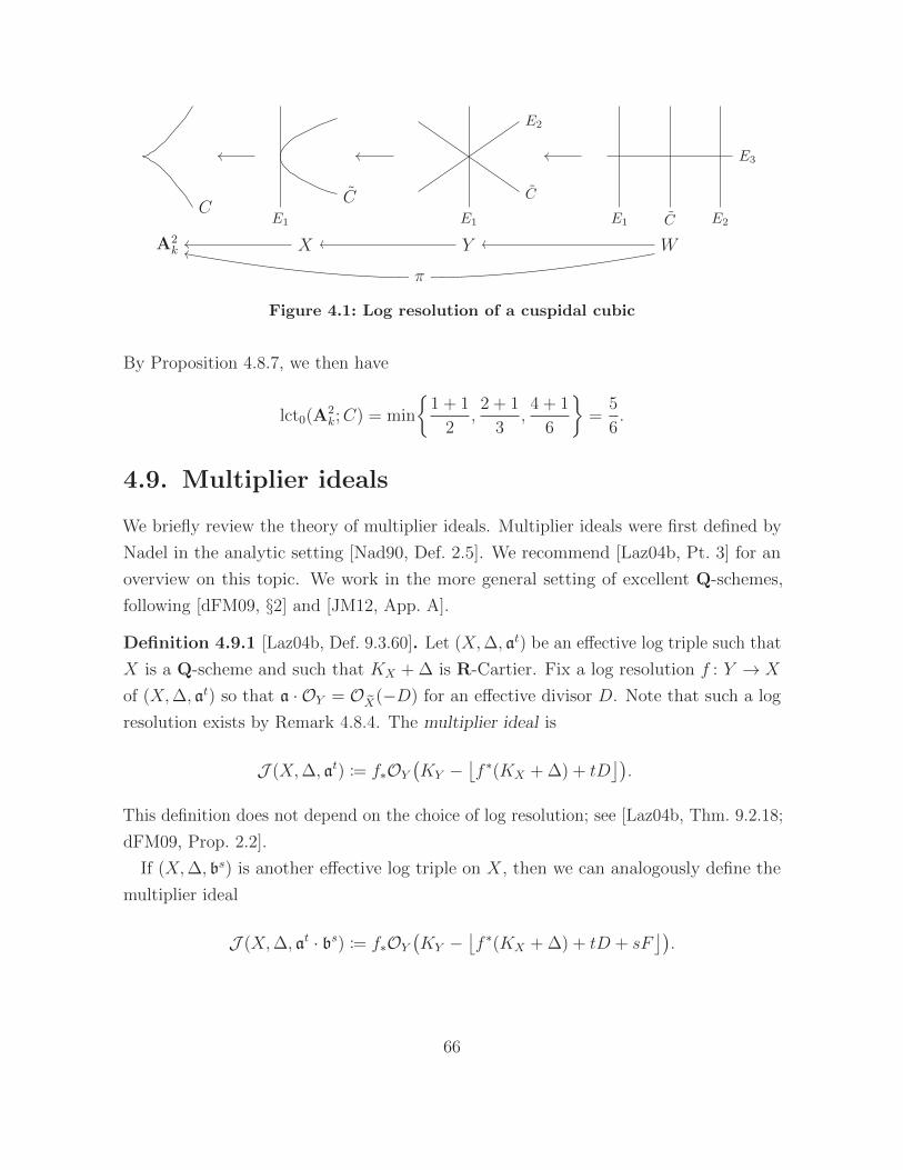
CC

E1 E1

C

E2

E3

E1 C E2

A2k X Y W

π

Figure 4.1: Log resolution of a cuspidal cubic

By Proposition 4.8.7, we then have

lct0(A2k;C) = min

1 + 1

2,2 + 1

3,4 + 1

6

=

5

6.

4.9. Multiplier ideals

We briefly review the theory of multiplier ideals. Multiplier ideals were first defined by

Nadel in the analytic setting [Nad90, Def. 2.5]. We recommend [Laz04b, Pt. 3] for an

overview on this topic. We work in the more general setting of excellent Q-schemes,

following [dFM09, §2] and [JM12, App. A].

Definition 4.9.1 [Laz04b, Def. 9.3.60]. Let (X,∆, at) be an effective log triple such that

X is a Q-scheme and such that KX + ∆ is R-Cartier. Fix a log resolution f : Y → X

of (X,∆, at) so that a · OY = OX(−D) for an effective divisor D. Note that such a log

resolution exists by Remark 4.8.4. The multiplier ideal is

J (X,∆, at) := f∗OY(KY −

⌊f ∗(KX + ∆) + tD

⌋).

This definition does not depend on the choice of log resolution; see [Laz04b, Thm. 9.2.18;

dFM09, Prop. 2.2].

If (X,∆, bs) is another effective log triple on X, then we can analogously define the

multiplier ideal

J (X,∆, at · bs) := f∗OY(KY −

⌊f ∗(KX + ∆) + tD + sF

⌋).

66

where f is a simultaneous log resolution for (X,∆, a) and (X,∆, b) such that b · OY =

OX(−F ) for an effective divisor F .

Note that if (X,∆, at) is an effective log triple such that X is a normal variety and

KX + ∆ is R-Cartier, then (X,∆, at) is klt if and only if J (X,∆, at) = OX [Laz04a, p.

165]. See [Laz04b, Ex. 9.2.30, Prop. 9.2.32, and p. 185] for some other basic properties

of multiplier ideals, which carry over to the setting of excellent Q-schemes. Some more

subtle properties in our context are checked in [dFM09, Prop. 2.3; JM12, App. A]. In

particular, the subadditivity theorem of Demailly–Ein–Lazarsfeld [DEL00, Thm. on p.

137] holds for regular excellent Q-schemes; see [JM12, Thm. A.2].

We will also need an asymptotic version of multiplier ideals for graded families of

ideals. Note that an asymptotic version of multiplier ideals first appeared in the work of

Siu [Siu98, pp. 668–669] in the analytic setting.

Definition 4.9.2 (see [Laz04a, Def. 11.1.15]). Let (X,∆, aλ•) be an effective log triple

such that X is a Q-scheme and such that KX + ∆ is R-Cartier. If m and r are positive

integers, then

J (X,∆, aλ/mm ) = J(X,∆, (arm)λ/(mr)

)⊆ J

(X,∆, aλ/(mr)mr

),

by [Laz04b, Rem. 9.2.4 and Prop. 9.2.32(iii)], and by the graded property arm ⊆ amr.

Thus, the set of ideals J (X,∆, aλ/mm )

∞m=1

(4.6)

is partially ordered, and has a unique maximal element by the noetherian property

that coincides with J (X,∆, aλ/mm ) for m sufficiently large and divisible. The asymptotic

multiplier ideal

J (X,∆, aλ•) ⊆ OX

is the maximal element of the partially ordered set (4.6).

If (X,∆, bλ•) is another effective log triple on X, then we can analogously define the

multiplier ideal J (X,∆, aλ• · bµ•).

The following examples of multiplier ideals will be the most useful in our applications.

Example 4.9.3 (see [Laz04b, Defs. 9.2.10 and 11.1.2]). Suppose (X,∆) is an effective

log pair where X is a complete scheme over a field of characteristic zero. If D is a Cartier

67

divisor such that H0(X,OX(mD)) 6= 0 for some positive integer m, then for every real

number t ≥ 0, we set

J(X,∆, t · |D|

):= J

(X,∆, b

(|D|)t).

If D is a Q-Cartier divisor such that H0(X,OX(mD)) 6= 0 for some sufficiently divisible

m > 0, then for every real number λ ≥ 0, we set

J(X,∆, λ · ‖D‖

):= J

(X,∆, a•(D)λ

),

where a•(D) is the graded family of ideals defined in Example 4.5.4.

Finally, we have the following uniform global generation result for the (asymptotic)

multiplier ideals defined in Example 4.9.3.

Theorem 4.9.4 (cf. [Laz04b, Prop. 9.4.26 and Cor. 11.2.13]). Let (X,∆) be an effective

log pair where X is a normal projective variety over a field k of characteristic zero and

∆ is an effective Q-Weil divisor such that KX + ∆ is Q-Cartier. Let D, L, and H be

Cartier divisors on X such that H is ample and free. If λ is a non-negative real number

such that L− (KX + ∆ + λ ·D) is ample, then the sheaves

J(X,∆, λ · |D|

)⊗OX(L+ dH) and J

(X,∆, λ · ‖D‖

)⊗OX(L+ dH)

are globally generated for every integer d > dimX.

Proof. By choosing n sufficiently divisible such that

J(X,∆, λ · ‖D‖

)= J

(X,∆, (λ/n) · |nD|

),

it suffices to consider the case for the usual multiplier ideals. Global generation follows

from Nadel vanishing when k is algebraically closed [Laz04b, Prop. 9.4.26 and Rem.

9.4.27], hence it suffices to reduce to this case.

Let π : X := X ×k k → X denote the base extension to the algebraic closure k of k.

Since the extension k ⊆ k is faithfully flat, the sheaf J (X,∆, λ · |D|) ⊗ OX(L + dH)

is globally generated if its pullback to X is globally generated. The pullback to X is

isomorphic to

J(X, π∗∆, λ · |π∗D|

)⊗OX(π∗L+ dπ∗H) (4.7)

68

since the formation of multiplier ideals commutes with faithfully flat base change [JM12,

Prop. 1.9]. Moreover, the R-Cartier divisor

π∗(L− (KX + ∆ + λ ·D)

)= π∗L− (KX + π∗∆ + λ · π∗D)

is ample and π∗H is ample and free by faithfully flat base change [EGAIV2, Cor. 2.7.2].

To apply the special case when k is algebraically closed, we note that while X may not

be irreducible, it is still the disjoint union of normal varieties [Mat89, Rem. on pp. 64–65].

Thus, by applying [Laz04b, Prop. 9.4.26 and Rem. 9.4.27] to each connected component

of X individually, we see that the sheaf in (4.7) is globally generated.

69

Chapter 5

Preliminaries in positive

characteristic

In this chapter, we review some preliminaries on commutative algebra and algebraic

geometry in positive characteristic. See [ST12] and [TW18] for overviews on the topic.

See also [PST17] and [Pat18] for more geometric applications.

The only new material is a new, short proof of the subadditivity theorem for test

ideals (Theorem 5.5.8), and some material on F -pure triples in §5.4.

5.1. Conventions on the Frobenius morphism

We start by establishing our conventions for the Frobenius morphism.

Definition 5.1.1. Let X be a scheme of characteristic p > 0. The (absolute) Frobenius

morphism is the morphism F : X → X of schemes given by the identity on points and

the p-power map

OX(U) F∗OX(U)

f fp

on structure sheaves for every open subset U ⊆ X. If R is a ring of characteristic

p > 0, we denote the corresponding ring homomorphism by F : R → F∗R. For every

integer e ≥ 0, the eth iterate of the Frobenius morphism is denoted by F e : X → X

and F e : R → F e∗R. If a ⊆ OX is a coherent ideal sheaf, we define the eth Frobenius

70

power a[pe] to be the inverse image of a under the eth iterate of the Frobenius morphism.

Locally, if a is generated by (hi)i∈I , then a[pe] is generated by (hpe

i )i∈I .

We note that the notation F e∗R is used to remind us that the R-algebra structure on

F e∗R is given by the ring homomorphism F e.

5.2. The pigeonhole principle

A surprisingly important fact in this thesis is the following combinatorial result based on

the pigeonhole principle.

Lemma 5.2.1 (cf. [HH02, Lem. 2.4(a)]). Let R be a commutative ring of characteristic

p > 0. Then, for any ideal a generated by n elements and for all non-negative integers e

and `, we have the sequence of inclusions

a`pe+n(pe−1)+1 ⊆ (a`+1)[pe] ⊆ a(`+1)pe . (5.1)

Moreover, if R is a regular local ring of dimension n and m is the maximal ideal of R,

then

m`pe+n(pe−1) 6⊆ (m`+1)[pe].

Proof. The second inclusion in (5.1) is clear by the definition of Frobenius powers. We

want to show the first inclusion. Let y1, y2, . . . , yn be a set of generators for a. The ideal

a`pe+n(pe−1)+1 is generated by all elements of the form

n∏

i=1

yaii such thatn∑

i=1

ai = `pe + n(pe − 1) + 1, (5.2)

and the ideal (a`+1)[pe] is generated by all elements of the form

n∏

i=1

ypebii such that

n∑

i=1

bi = `+ 1. (5.3)

We want to show that the elements (5.2) are divisible by some elements of the form (5.3).

By the division algorithm, we may write ai = ai,0 + pea′i for some non-negative integers

71

ai,0 and a′i such that 0 ≤ ai,0 ≤ pe − 1. We then have

n∏

i=1

yaii =n∏

i=1

yai,0i ·

n∏

i=1

ypea′ii ,

and since ai,0 ≤ pe− 1, we have that∑n

i=1 ai,0 ≤ n(pe− 1). Thus, we have the inequality

`pe + n(pe − 1) + 1 =n∑

i=1

ai ≤ n(pe − 1) +n∑

i=1

pea′i,

which implies `+ p−e ≤∑ni=1 a

′i. Since the right-hand side of this inequality is an integer,

we have that `+ 1 ≤∑ni=1 a

′i, i.e., the element

∏ni=1 y

pea′ii is divisible by one of the form

(5.3). Thus, each element of the form in (5.2) is divisible by one of the form in (5.3).

Now suppose R is a regular local ring of dimension n, and m is the maximal ideal of

R. Let y1, y2, . . . , yn be a regular system of parameters. Then, we have

y`pe

i0·n∏

i=1

ype−1i ∈ m`pe+n(pe−1)

for all i0 ∈ 1, 2, . . . , n. This monomial does not lie in (m`+1)[pe] since its image is not in

the extension of (m`+1)[pe] in the completion of R at m, which is isomorphic to a formal

power series ring with variables y1, y2, . . . , yn by the Cohen structure theorem.

We moreover show that asymptotically, the number n of elements generating a can be

replaced by the analytic spread of a. See [HS06, Def. 5.1.5] for the definition of analytic

spread.

Lemma 5.2.2. Let (R,m, k) be a noetherian local ring of characteristic p > 0. Then,

for every ideal a of analytic spread h, there exists an integer t ≥ 0 such that for all

non-negative integers e and `, we have the sequence of inclusions

a`pe+h(pe−1)+1+t ⊆ (a`+1)[pe] ⊆ a(`+1)pe . (5.4)

In particular, if a = m, then (5.4) holds for h = dimR.

Proof. The right inclusion in (5.4) is clear as in Lemma 5.2.1. It therefore suffices to prove

the left inclusion in (5.4). We first reduce to the case when k is infinite. Consider the

72

ring S = R[x]mR[x] as in [HS06, §8.4]. Then, S is a noetherian local ring of characteristic

p > 0 such that R ⊆ S is faithfully flat and S/mS ' k(x) is infinite. Since we can check

the inclusions in (5.4) after a faithfully flat extension [Mat89, Thm. 7.5(ii)], and since

analytic spread does not change after passing to S [HS06, Lem. 8.4.2(4)], we can replace

R with S to assume that k is infinite.

We now prove the left inclusion in (5.4) under the assumption that k is infinite. Recall

that since k is infinite, there exists an ideal q ⊆ a called a minimal reduction ideal and

an integer t > 0 such that q is generated by h elements, and as+t = qs · at for every

integer s ≥ 0; see [HS06, Def. 1.2.1 and Prop. 8.3.7]. Setting s = `pe + h(pe − 1) + 1, we

have

a`pe+h(pe−1)+1+t = q`p

e+h(pe−1)+1 · at ⊆ (q`+1)[pe] · at ⊆ (a`+1)[pe]

for all non-negative integers e and `, where the first inclusion holds by Lemma 5.2.1.

The special case for a = m follows from [HS06, Cor. 8.3.9].

5.3. F -finite schemes

As mentioned in §2.4, in positive characteristic, one often needs to restrict or reduce to

the case when the Frobenius morphism is finite. We isolate this class of schemes.

Definition 5.3.1. Let X be a scheme of characteristic p > 0. We say that X is F -finite

if the (absolute) Frobenius morphism F : X → X is finite. We say that a ring R of

characteristic p > 0 is F -finite if SpecR is F -finite, or equivalently if F : R → F∗R is

module-finite.

Note that a field k is F -finite if and only if [k : kp] < ∞. F -finite schemes are

ubiquitous in geometric contexts because of the following:

Example 5.3.2 (see [Kun76, p. 999; BMS08, Ex. 2.1]). If X is a scheme that is locally

essentially of finite type over an F -finite scheme of characteristic p > 0, then X is F -finite.

In particular, schemes essentially of finite type over perfect or F -finite fields are F -finite.

If a scheme X of characteristic p > 0 is F -finite, then Grothendieck duality (Theo-

rem 4.4.1) can be applied to the Frobenius morphism since it is finite. The F -finiteness

condition implies other desirable conditions as well.

73

Theorem 5.3.3 [Kun76, Thm. 2.5; Gab04, Rem. 13.6]. Let R be a noetherian F -finite

ring of characteristic p > 0. Then, R is excellent and is isomorphic to a quotient of a

regular ring of finite Krull dimension. In particular, R admits a dualizing complex.

See [Har66, Def. on p. 258] for the definition of a dualizing complex.

5.4. F -singularities of pairs and triples

We now define F -singularities for log triples in the sense of Definition 4.7.1. These are

common generalizations of the notions for log pairs (X,∆) and (X, at) due to Hara–

Watanabe [HW02] and Takagi [Tak04b], respectively. While an equivalent definition

of strong F -regular triples has appeared before (see Example 5.4.5), the definition of

F -pure triples appears to be new.

We note that we assume F -finiteness throughout. See Appendix A for an overview on

F -singularities for rings, where we work without F -finiteness assumptions.

Definition 5.4.1 (cf. [HW02, Def. 2.1; Tak04b, Def. 3.1]). Let (R,∆, at) be an effective

log triple such that R is an F -finite local ring of characteristic p > 0.

(a) The triple (R,∆, at) is F -pure if there exists an integer e′ > 0 such that for all

e ≥ e′, there exists an element d ∈ ab(pe−1)tc for which the composition

RF e−→ F e

∗R −→ F e∗R(b(pe − 1)∆c

) F e∗ (−·d)−−−−→ F e∗R(b(pe − 1)∆c

)(5.5)

splits as an R-module homomorphism.

(b) The triple (R,∆, at) is sharply F -pure if there exists an integer e > 0 and an

element d ∈ ad(pe−1)te for which the composition

RF e−→ F e

∗R −→ F e∗R(d(pe − 1)∆e

) F e∗ (−·d)−−−−→ F e∗R(d(pe − 1)∆e

)(5.6)

splits as an R-module homomorphism.

(c) The triple (R,∆, at) is strongly F -regular if for all c ∈ R, there exists an integer

e > 0 and an element d ∈ ab(pe−1)tc for which the composition

RF e−→ F e

∗R −→ F e∗R(b(pe − 1)∆c

) F e∗ (−·cd)−−−−−→ F e∗R(b(pe − 1)∆c

)(5.7)

74

splits as an R-module homomorphism.

Now suppose that (X,∆, at) is an effective log triple such that X is an F -finite scheme

of characteristic p > 0, and let x ∈ X be a point. The triple (X,∆, at) is F -pure (resp.

sharply F -pure, strongly F -regular) at x if the localized triple (OX,x,∆|SpecOX,x , atx) is

F -pure (resp. sharply F -pure, strongly F -regular). The triple (X,∆, at) is F -pure (resp.

sharply F -pure, strongly F -regular) if it is F -pure (resp. strongly F -regular) at every

point x ∈ X.

Remark 5.4.2. A triple (R, 0, R1) as in Definition 5.4.1 is F -pure if and only if R is

F -pure in the sense of Hochster–Roberts (since F -purity and F -splitting coincide F -finite

rings; see Figure A.1), and is strongly F -regular if and only if R is strongly F -regular in

the sense of Hochster–Huneke (Definition A.7(a)).

We collect some basic properties of F -singularities for triples.

Proposition 5.4.3 (cf. [HW02, Prop. 2.2; Tak04b, Prop. 3.3]). Let (R,∆, at) be an

effective log triple such that R is an F -finite local ring of characteristic p > 0.

(i) If (R,∆, at) is F -pure (resp. sharply F -pure, strongly F -regular), then so is

(R,∆′, bs) for every triple such that ∆′ ≤ ∆, b ⊇ a, and s ∈ [0, t].

(ii) If (R,∆, at) is F -pure, then d∆e is reduced, i.e., the nonzero coefficients of d∆eare equal to 1.

(iii) (R,∆, at) is strongly F -regular if and only if for all c ∈ R, there exists an integer

e′ > 0 such that for all e ≥ e′, there exists d ∈ adpete for which the composition

RF e−→ F e

∗R −→ F e∗R(dpe∆e

) F e∗ (−·cd)−−−−−→ F e∗R(dpe∆e

)(5.8)

splits as an R-module homomorphism.

(iv) We have the implications

strongly F -regular sharply F -pure

F -pure

where the dashed implication holds when ∆ is Cartier and a is locally principal.

75

Proof. (i) follows since the splitting conditions for (R,∆′, bs) are weaker than those for

(R,∆, at). For (ii), we note that (R,∆) is F -pure by (i), hence (ii) follows from [HW02,

Prop. 2.2(4)].

For (iii), we note that ⇐ is clear. For ⇒, the case when ∆ = 0 is shown in [Tak04b,

Prop. 3.3(3)], hence it suffices to consider when ∆ 6= 0, in which case R is a normal

domain by our conventions in Definition 4.7.1. Let c′ ∈ R be arbitrary; we want to show

that for c = c′, the composition (5.8) splits for some d ∈ adpete for all e 0. Choose

nonzero elements a ∈ R(−2d∆e) and b ∈ a2dte, in which case

a ·R(dpe∆e

)⊆ R

(dpe∆e − 2d∆e

)⊆ R

(b(pe − 1)∆c

)

b · ab(pe−1)tc ⊆ a2dte+b(pe−1)tc ⊆ adpete

for every integer e > 0. By the assumption that (R,∆, at) is strongly F -regular, there

exist e′ > 0 and d′ ∈ ab(pe′−1)tc such that the composition (5.7) splits for e = e′ and with

c = abc′. This composition factors as

RF e′

−→ F e′∗ R −→ F e′

∗ R(dpe′∆e

)

F e′∗ (−·bc′d′)−−−−−−−→ F e′

∗ R(dpe′∆e

) F e′∗ (−·a)−−−−−→ F e′

∗ R(b(pe′ − 1)∆c

),

hence the composition of the first three homomorphisms splits. Now since R is F -pure

by (i), the homomorphism

F e′∗ R(dpe′∆e

) F e′∗ (F e−e

′(dpe′∆e))−−−−−−−−−−−→ F e

∗R(pe−e

′dpe′∆e),

which is obtained by twisting the (e− e′)th iterate of the Frobenius homomorphism by

dpe′∆e and applying F e′∗ , also splits for every e ≥ e′. The composition

RF e′

−→ F e′∗ R −→ F e′

∗ R(dpe′∆e

) F e′∗ (−·bc′d′)−−−−−−−→ F e′

∗ R(dpe′∆e

)

F e′∗ (F e−e

′(dpe′∆e))−−−−−−−−−−−→ F e

∗R(pe−e

′dpe′∆e)

76

therefore splits for e ≥ e′. Finally, this composition factors as

RF e−→ F e

∗R −→ F e∗R(dpe∆e

) F e∗ (−·(bc′d′)pe−e′)−−−−−−−−−−→ F e

∗R(dpe∆e

)−→ F e

∗R(pe−e

′dpe′∆e),

hence the composition (5.8) splits for c = c′ and

d = bpe−e′

(c′)pe−e′−1(d′)p

e−e′ ∈(a2dte+b(pe′−1)tc)pe−e′ ⊆

(adp

e′ te)pe−e′ ⊆ adpete.

Finally, for (iv), we note that strong F -regularity implies sharp F -purity by (iii), and

the dashed implication holds by [Sch08, Prop. 3.5].

Remark 5.4.4. It seems to be unknown whether sharp F -purity implies F -purity in

general [Sch08, Ques. 3.8].

Example 5.4.5. While Proposition 5.4.3(iii) shows that the rounding “b(pe − 1)−c” in

Definition 5.4.1(c) can be replaced by “d(pe − 1)−e” (this is the convention in [Sch10b,

Def. 2.11; Sch10a, Def. 3.2]), this is not the case for F -purity. For example, the pair

(F2Jx, y, zK, (x2 + y5 + z5)1/2

)

from [MY09, Ex. 4.3] is F -pure but not sharply F -pure by [Her12, Thm. 4.1].

5.4.1. The trace of Frobenius

We now describe variants of the Grothendieck trace map associated to the Frobenius

morphism, and its relationship to F -singularities. This material is essentially contained

in [Sch09a], although we use some of the notation of [Tan15, §2] and [CTX15, §2.3].

Proposition 5.4.6 [CTX15, Def.-Prop. 2.5]. Let X be a normal scheme essentially of

finite type over an F -finite field of characteristic p > 0, let D be an effective Weil divisor

on X, and let e be a positive integer. Then, there exists a homomorphism

TreX,D : F e∗(OX((1− pe)KX −D

))−→ OX

77

of OX-modules that fits into a commutative diagram

F e∗(OX((1− pe)KX −D

))OX

HomOX(F e∗(OX(D)

),OX

)HomOX (OX ,OX)

TreX,D

θ

∼ ∼

(F eD)∗

(5.9)

of OX-modules, where the left vertical arrow is an isomorphism of (F e∗OX ,OX)-bimodules

and the right vertical arrow is an isomorphism of OX-modules.

Proof. Consider the composition map

OX F e−→ F e∗OX −→ F e

∗OX(D),

which we denote by F eD. Applying the contravariant functor HomOX (−,OX), we have

the top arrow in the commutative diagram

HomOX(F e∗(OX(D)

),OX

)HomOX (OX ,OX)

HomOX(F e∗(OX(peKX +D)

),OX(KX)

)HomOX

(OX(KX),OX(KX)

)

(F eD)∗

∼ ∼where the vertical arrows are isomorphisms by restricting to the regular locus of X, by

the fact that OX(KX) is a reflexive sheaf, and by Lemma 4.3.3 and Theorem 4.3.5. By

Grothendieck duality for finite morphisms (see Theorem 4.4.1), the sheaf in the bottom

left corner satisfies

HomOX(F e∗(OX(peKX +D)

),OX(KX)

)' F e

∗ HomOX(OX(peKX +D), F e!OX(KX)

)

' F e∗ HomOX

(OX(peKX +D),OX(KX)

)

' F e∗OX

((1− pe)KX −D

)

where the second isomorphism follows from the fact that F e!ωX ' ωX by Definition 4.4.2

and Theorem 4.4.1, and the last isomorphism follows from restricting to the regular

locus of X and using the reflexivity of the sheaves involved [Har94, Prop. 2.7]. We can

78

therefore define θ to be the composition of isomorphisms

F e∗OX

((1− pe)KX −D

)'HomOX

(F e∗(OX(peKX +D)

),OX(KX)

)

'HomOX(F e∗(OX(D)

),OX

).

Note that θ is an isomorphism of left-F e∗OX-modules by tracing through these isomor-

phisms, where the left-F e∗OX-module structure comes from precomposition by multipli-

cation by an element in F e∗OX .

We then use Proposition 5.4.6 to prove the following characterization of F -singularities.

Corollary 5.4.7. Let (X,∆, at) be an effective log triple such that X is F -finite and of

characteristic p > 0.

(i) The triple (X,∆, at) is F -pure if and only if there exists an integer e′ > 0 such that

for all e ≥ e′, the morphism

F e∗(ab(p

e−1)tc · OX((1− pe)KX − b(pe − 1)∆c

))

−→ F e∗(OX((1− pe)KX − b(pe − 1)∆c

)) TreX,b(pe−1)∆c−−−−−−−−→ OX

is surjective.

(ii) The triple (X,∆, at) is sharply F -pure if and only if there exists an integer e > 0

such that the morphism

F e∗(ad(p

e−1)te · OX((1− pe)KX − d(pe − 1)∆e

))

−→ F e∗(OX((1− pe)KX − d(pe − 1)∆e

)) TreX,d(pe−1)∆e−−−−−−−−→ OX

is surjective.

(iii) The triple (X,∆, at) is strongly F -regular if and only if for every Cartier divisor E

on X, there there exists an integer e > 0 such that the morphism

F e∗(ab(p

e−1)tc · OX((1− pe)KX − b(pe − 1)∆c − E

))

−→ F e∗(OX((1− pe)KX − b(pe − 1)∆c − E

)) TreX,b(pe−1)∆c+E−−−−−−−−−→ OX

79

is surjective.

Proof. We first consider the case of a pair (X,∆). Let D stand for one of b(pe − 1)∆c,d(pe − 1)∆e, or b(pe − 1)∆c+E. By Proposition 5.4.6, we see that TreX,D is surjective if

and only if

(F eD)∗ : HomOX

(F e∗(OX(D)

),OX

)−→HomOX (OX ,OX)

is surjective. Since X is F -finite, these morphisms are surjective if and only if for every

x ∈ X, the morphism

(F eD)∗ : HomOX,x

(F e∗(OX,x(D)

),OX,x

)−→ HomOX,x(OX,x,OX,x)

is surjective. Finally, this condition is equivalent to the splitting of the map

OX,x −→ F e∗OX,x −→ F e

∗(OX,x(D)

),

hence all three statements follow by comparing this condition to Definition 5.4.1.

Finally, the case for a triple (X,∆, at) follows from the fact that under the isomorphism

θ in Proposition 5.4.6, the multiplication F e∗ (− · d) or F e

∗ (− · cd) in Definition 5.4.1

corresponds to precomposition of the trace TreX,D by multiplication by an element in

ab(pe−1)tc or ad(p

e−1)te.

5.4.2. F -pure thresholds

We define the F -pure threshold, which is the positive characteristic analogue of the log

canonical threshold.

Definition 5.4.8 [TW04, Def. 2.1]. Let (X,∆, a) be an effective log triple such that X

is F -finite of characteristic p > 0. The F -pure threshold of the pair (X,∆) with respect

to a at a point x ∈ X is

fptx((X,∆); a

):= sup

c ∈ R≥0

∣∣ the triple (X,∆, ac) is F -pure at x,

where if (X,∆) is not F -pure at x, then we set fptx((X,∆); a) = −∞.

80

F -pure thresholds can be very different from log canonical thresholds, even for the

same defining equation.

Example 5.4.9 [MTW05, Ex. 4.3]. Let R = kJx, yK with maximal ideal m, where k is

an F -finite field of characteristic p > 0, and let f = x2 + y3. The F -pure threshold then

depends on the characteristic of k:

fptm(SpecR;x2 + y3

)=

1

2if p = 2

2

3if p = 3

5

6if p ≡ 1 mod 3

5

6− 1

6pif p ≡ 2 mod 3 and p 6= 2

We see that as p → ∞, the F -pure threshold approaches the log canonical threshold

as computed in Example 4.8.8, as predicted by Theorem 5.6.8. For more examples of

similar phenomena, see [TW04, Exs. 2.4 and 2.5; MTW05, §4; CHSW16].

5.5. Test ideals

We review the theory of test ideals, which are the positive characteristic analogues of

multiplier ideals. Test ideals for rings were originally defined by Hochster and Huneke

[HH90, Def. 8.22] using tight closure, and versions for pairs and triples were first defined

by Hara–Yoshida [HY03, Def.-Thm. 6.5] and Takagi [Tak04a, Def. 2.6; Tak08, Def. 2.2]

using generalized versions of tight closure; see Remark 5.5.14. While test ideals can

be defined in this way without F -finiteness assumptions, we will assume F -finiteness

throughout and define test ideals using the notion of F -compatibility, following Schwede

[Sch10b]. We recommend [ST12, §6; TW18, §5] for surveys on this topic.

We start with the following definition.

Definition 5.5.1 [Sch10b, Def. 3.1]. Let (R,∆, at) be an effective log triple such that

R is an F -finite ring of characteristic p > 0. An ideal J ⊆ R is uniformly (∆, at, F )-

compatible if for every integer e > 0 and every ϕ ∈ HomR(F e∗R(d(pe − 1)∆e), R), we

81

have

ϕ(F e∗(J · adt(pe−1)e)) ⊆ J. (5.10)

We drop ∆ or at from our notation when working with pairs or the ring itself.

If (R,∆, bs) is another effective log triple on R, then we can analogously define uniform

(∆, at · bs, F )-compatibility by using the ideal adt(pe−1)e · bds(pe−1)e in (5.10).

We can now define test ideals.

Definition 5.5.2 [Sch10b, Def. 3.1 and Thm. 6.3]. Let (R,∆, at) be an effective log

triple such that R is an F -finite ring of characteristic p > 0. The test ideal

τ(R,∆, at) ⊆ R

is the smallest ideal which is uniformly (∆, at, F )-compatible and whose intersection with

R is nonempty. We drop ∆ or at from our notation when working with pairs or the

ring itself. We also often drop the ring R from our notation if it is clear from context.

If (R,∆, bs) is another effective log triple on R, then we can analogously define the

test ideal τ(R,∆, at · bs) as the smallest uniformly (∆, at · bs, F )-compatible ideal that

intersects R.

The test ideal as defined in Definition 5.5.2 exists since it matches the earlier notion

(see Remark 5.5.14) defined using tight closure [Sch10b, Thm. 6.3]. We briefly describe a

direct proof of existence, following [Sch11]. The key ingredient is the following:

Definition 5.5.3 (cf. [Sch11, Def. 3.19]). Let (R,∆, at) be an effective log triple such

that R is an F -finite ring of characteristic p > 0. An element c ∈ R is a big sharp test

element for (R,∆, at) if, for every d ∈ R, there exists ϕ ∈ HomR(F e∗R(d(pe − 1)∆e), R)

for some integer e > 0 such that

c ∈ ϕ(F e∗(d · adt(pe−1)e)). (5.11)

If c is a big sharp test element, then c′c is also for all c′ ∈ R by considering the

composition (c′ · −) ϕ for ϕ as in (5.11).

If (R,∆, bs) is another effective log triple on R, then we can analogously define the big

sharp test elements for (R,∆, at) and (R,∆, bs) by using the ideal adt(pe−1)e · bds(pe−1)e in

(5.11).

82

Various versions of test elements were shown to exist in the context of tight closure;

see [HH90, §6; HY03, Thm. 6.4; Tak04a, Thm. 2.5(2); Hoc07, Thm. on p. 90]. Big sharp

test elements as defined in Definition 5.5.3 exist by [Sch10b, Lem. 2.17; Sch11, Prop.

3.21]. Assuming this fact, we can show that test ideals exist. Note that the description

(5.12) is originally due to Hara and Takagi [HT04, Lem. 2.1].

Theorem 5.5.4 [Sch11, Thm. 3.18]. Let (R,∆, at) be an effective log triple such that

R is an F -finite ring of characteristic p > 0. Then, for every choice of big sharp test

element c ∈ R for the triple (R,∆, at), we have

τ(R,∆, at) =∞∑

e=0

∑

ϕe

ϕe

(F e∗(c · adt(pe−1)e)), (5.12)

where ϕe ranges over all elements in HomR(F e∗R(d(pe− 1)∆e), R). In particular, the test

ideal τ(R,∆, at) exists. If (R,∆, bs) is another effective log triple, then τ(R,∆, at · bs)exists by replacing c with a big sharp test element for (R,∆, at) and (R,∆, bs) and by

using the ideal adt(pe−1)e · bds(pe−1)e in (5.12).

Proof. By definition of a big sharp test element (Definition 5.5.3), we have c ∈ J for

every (∆, at, F )-compatible ideal J ⊆ R. On the other hand, the ideal on the right-hand

side of (5.12) is the smallest (∆, at, F )-compatible ideal containing c, hence must coincide

with τ(R,∆, at). The proof for τ(R,∆, at · bs) is similar.

To define test ideals on schemes, we use the following consequence of the proof of the

existence of big sharp test elements.

Proposition 5.5.5 [Sch11, Prop. 3.23(ii)]. Let (R,∆, at) be an effective log triple such

that R is an F -finite ring of characteristic p > 0. For every multiplicative set W ⊆ R,

we have

W−1 τ(R,∆, at) = τ(W−1R,∆|SpecW−1R, (W

−1a)t),

and similarly for τ(R,∆, at · bs).

We can now define test ideals on schemes.

Definition 5.5.6. Let (X,∆, at) be an effective log triple such that X is an F -finite

scheme of characteristic p > 0. By Proposition 5.5.5, we can define the test ideal

83

τ(X,∆, at) ⊆ OX locally on every open affine subset U = SpecR ⊆ X by

τ(X,∆, at)(U) = τ(R,∆|U , a(U)t

).

We drop ∆ or at from our notation when working with pairs or the scheme itself. We

also often drop the scheme X from our notation if it is clear from context.

If (X,∆, bs) is another effective log triple on X, then we can analogously define the

test ideal τ(X,∆, at · bs).

We now state some properties of test ideals that we will use often, which are reminiscent

of those for multiplier ideals in [Laz04b, §9.2].

Proposition 5.5.7 (see [TW18, Prop. 5.6]). Let (X,∆, at) be an effective log triple such

that X is an F -finite scheme of characteristic p > 0.

(i) If (X, b) is a log pair on X, then τ(∆, at) · b ⊆ τ(∆, at · b).

(ii) Let (X,∆′, bs) be another effective log triple on X. If ∆ ≥ ∆′ and adt(pe−1)e ⊆

bds(pe−1)e for every integer e > 0, then τ(∆, at) ⊆ τ(∆′, bs).

(iii) For every non-negative real number s, we have τ(∆, as · at) = τ(∆, as+t).

(iv) For every non-negative integer m, we have τ(∆, (am)t) = τ(∆, amt).

(v) There exists ε > 0 such that for all s ∈ [t, t+ ε], we have τ(∆, at) = τ(∆, as).

(vi) Suppose that X is normal. For every effective Cartier divisor D on X, there exists

ε > 0 such that for all δ ∈ [0, ε], we have τ(∆, at) = τ(∆ + δD, at).

(vii) The triple (X,∆, at) is strongly F -regular if and only if τ(∆, at) = OX .

We will define strong F -regularity in Definition 5.4.1(c).

Proof. Since test ideals are defined locally, it suffices to consider the case when X =

SpecR. Fix a big sharp test element c ∈ R. We will freely use the description of the

test ideal in Theorem 5.5.4.

84

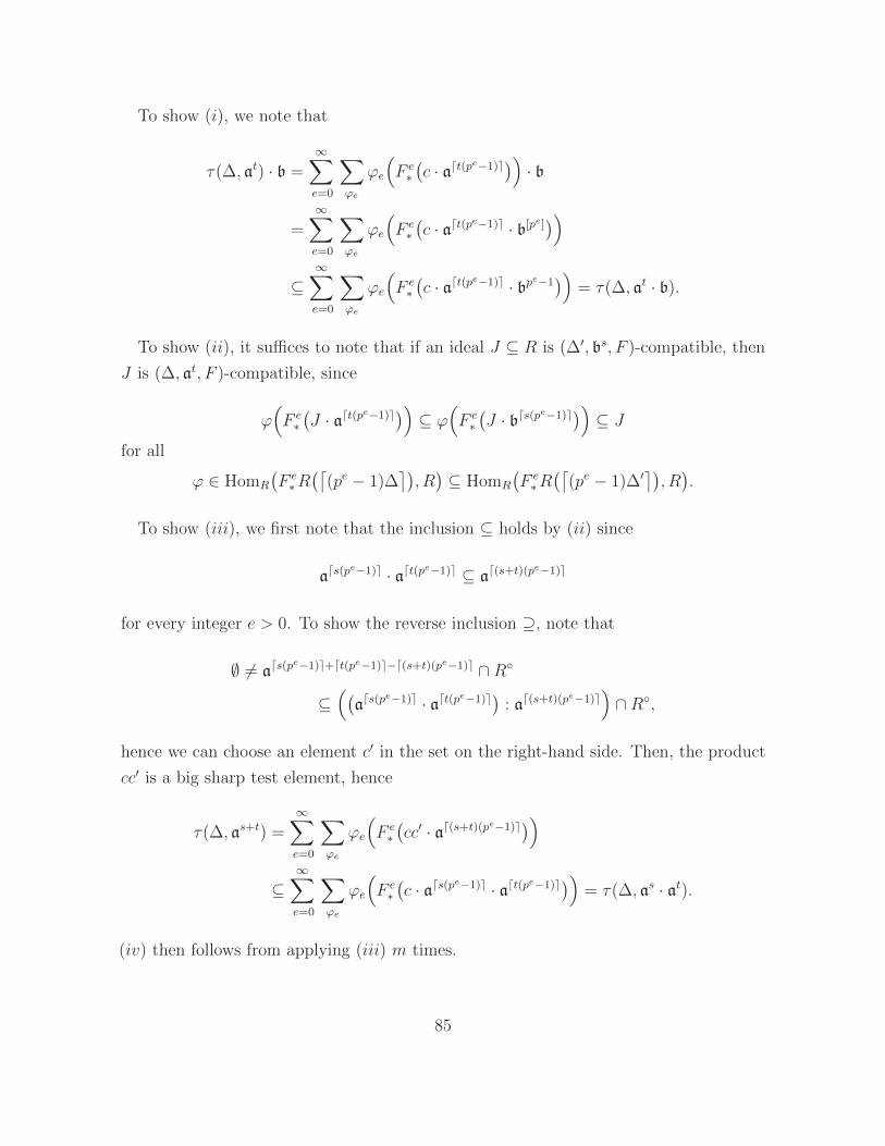
To show (i), we note that

τ(∆, at) · b =∞∑

e=0

∑

ϕe

ϕe

(F e∗(c · adt(pe−1)e)) · b

=∞∑

e=0

∑

ϕe

ϕe

(F e∗(c · adt(pe−1)e · b[pe]

))

⊆∞∑

e=0

∑

ϕe

ϕe

(F e∗(c · adt(pe−1)e · bpe−1

))= τ(∆, at · b).

To show (ii), it suffices to note that if an ideal J ⊆ R is (∆′, bs, F )-compatible, then

J is (∆, at, F )-compatible, since

ϕ(F e∗(J · adt(pe−1)e)) ⊆ ϕ

(F e∗(J · bds(pe−1)e)) ⊆ J

for all

ϕ ∈ HomR

(F e∗R(⌈

(pe − 1)∆⌉), R)⊆ HomR

(F e∗R(⌈

(pe − 1)∆′⌉), R).

To show (iii), we first note that the inclusion ⊆ holds by (ii) since

ads(pe−1)e · adt(pe−1)e ⊆ ad(s+t)(p

e−1)e

for every integer e > 0. To show the reverse inclusion ⊇, note that

∅ 6= ads(pe−1)e+dt(pe−1)e−d(s+t)(pe−1)e ∩R

⊆((

ads(pe−1)e · adt(pe−1)e) : ad(s+t)(p

e−1)e)∩R,

hence we can choose an element c′ in the set on the right-hand side. Then, the product

cc′ is a big sharp test element, hence

τ(∆, as+t) =∞∑

e=0

∑

ϕe

ϕe

(F e∗(cc′ · ad(s+t)(pe−1)e))

⊆∞∑

e=0

∑

ϕe

ϕe

(F e∗(c · ads(pe−1)e · adt(pe−1)e)) = τ(∆, as · at).

(iv) then follows from applying (iii) m times.

85

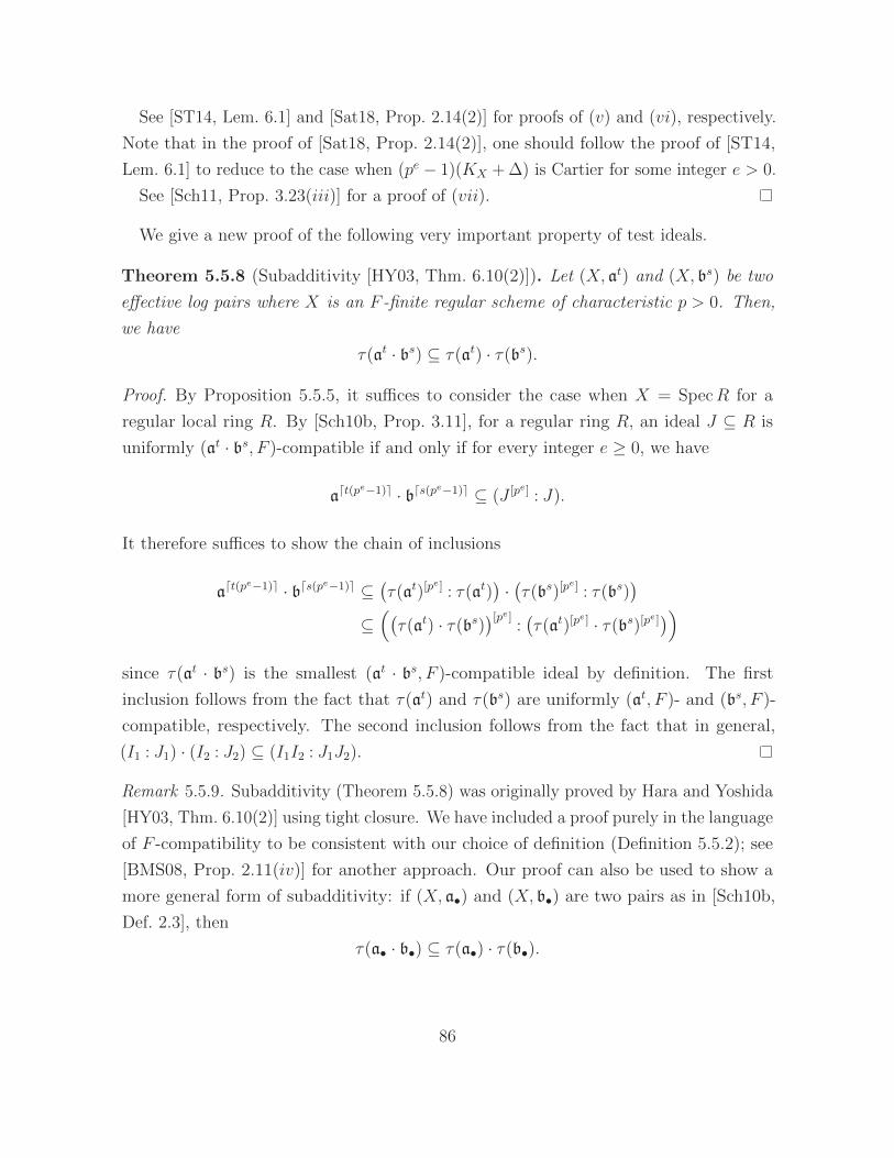
See [ST14, Lem. 6.1] and [Sat18, Prop. 2.14(2)] for proofs of (v) and (vi), respectively.

Note that in the proof of [Sat18, Prop. 2.14(2)], one should follow the proof of [ST14,

Lem. 6.1] to reduce to the case when (pe − 1)(KX + ∆) is Cartier for some integer e > 0.

See [Sch11, Prop. 3.23(iii)] for a proof of (vii).

We give a new proof of the following very important property of test ideals.

Theorem 5.5.8 (Subadditivity [HY03, Thm. 6.10(2)]). Let (X, at) and (X, bs) be two

effective log pairs where X is an F -finite regular scheme of characteristic p > 0. Then,

we have

τ(at · bs) ⊆ τ(at) · τ(bs).

Proof. By Proposition 5.5.5, it suffices to consider the case when X = SpecR for a

regular local ring R. By [Sch10b, Prop. 3.11], for a regular ring R, an ideal J ⊆ R is

uniformly (at · bs, F )-compatible if and only if for every integer e ≥ 0, we have

adt(pe−1)e · bds(pe−1)e ⊆ (J [pe] : J).

It therefore suffices to show the chain of inclusions

adt(pe−1)e · bds(pe−1)e ⊆

(τ(at)[pe] : τ(at)

)·(τ(bs)[pe] : τ(bs)

)

⊆((τ(at) · τ(bs)

)[pe]:(τ(at)[pe] · τ(bs)[pe]

))

since τ(at · bs) is the smallest (at · bs, F )-compatible ideal by definition. The first

inclusion follows from the fact that τ(at) and τ(bs) are uniformly (at, F )- and (bs, F )-

compatible, respectively. The second inclusion follows from the fact that in general,

(I1 : J1) · (I2 : J2) ⊆ (I1I2 : J1J2).

Remark 5.5.9. Subadditivity (Theorem 5.5.8) was originally proved by Hara and Yoshida

[HY03, Thm. 6.10(2)] using tight closure. We have included a proof purely in the language

of F -compatibility to be consistent with our choice of definition (Definition 5.5.2); see

[BMS08, Prop. 2.11(iv)] for another approach. Our proof can also be used to show a

more general form of subadditivity: if (X, a•) and (X, b•) are two pairs as in [Sch10b,

Def. 2.3], then

τ(a• · b•) ⊆ τ(a•) · τ(b•).

86

Here, the test ideal is as described in [Sch11, Thm. 6.3]. We have avoided this notation

since it clashes with that of asymptotic test ideals below.

Because of the formal properties of test ideals in Proposition 5.5.7, we can define the

following asymptotic version of test ideals.

Definition 5.5.10 [Sat18, Prop.-Def. 2.16]. Let (X,∆, aλ•) be an effective log triple such

that X is F -finite and of characteristic p > 0. If m and r are positive integers, then

τ(X,∆, aλ/mm ) = τ(X,∆, (arm)λ/(mr)

)⊆ τ

(X,∆, aλ/(mr)mr

),

by Propositions 5.5.7(iv) and 5.5.7(ii), and by the graded property arm ⊆ amr. Thus, the

set of ideals τ(X,∆, aλ/mm )

∞m=1

(5.13)

is partially ordered, and has a unique maximal element by the noetherian property that

coincides with τ(X,∆, aλ/mm ) for m sufficiently large and divisible. The asymptotic test

ideal

τ(X,∆, aλ•) ⊆ OX

is the maximal element of the partially ordered set (5.13).

If (X,∆, bµ•) is another effective log triple on X, then we can analogously define the

test ideal τ(X,∆, aλ• · bµ•).

Asymptotic test ideals satisfy properties analogous to those in Proposition 5.5.7

and Theorem 5.5.8.

Remark 5.5.11. Definition 5.5.10 is due to Mustata when X is regular and ∆ = 0 [Mus13,

pp. 540–541]. An asymptotic version of the test ideal was first defined by Hara [Har05,

Prop.-Def. 2.9], although this ideal differs from that in Definition 5.5.10 in general; see

[TY08, Rem. 1.4].

The following examples of test ideals will be the most useful in our applications.

Example 5.5.12 (see [Sat18, Def. 2.36]). Suppose (X,∆) is an effective log pair where

X is a complete scheme over an F -finite field of characteristic p > 0. If D is a Cartier

divisor such that H0(X,OX(D)) 6= 0, then for every real number t ≥ 0, we set

τ(X,∆, t · |D|

):= τ

(X,∆, b

(|D|)t).

87

If D is a Q-Cartier divisor such that H0(X,OX(mD)) 6= 0 for some m > 0 such that

mD is Cartier, then for every real number λ ≥ 0, we set

τ(X,∆, λ · ‖D‖

):= τ

(X,∆, a•(D)λ

),

where a•(D) is the graded family of ideals defined in Example 4.5.4.

Finally, we have the following uniform global generation result for (asymptotic) test

ideals.

Theorem 5.5.13 ([Sat18, Prop. 4.1]; cf. [Sch14, Thm. 4.3; Mus13, Thm. 4.1]). Let

(X,∆) be an effective log pair where X is a normal projective variety over an F -finite

field of characteristic p > 0 and ∆ is an effective Q-Weil divisor such that KX + ∆ is

Q-Cartier. Let D, L, and H be Cartier divisors on X such that H is ample and free.

If λ is a non-negative real number such that L− (KX + ∆ + λ ·D) is ample, then the

sheaves

τ(X,∆, λ · |D|

)⊗OX(L+ dH) and τ

(X,∆, λ · ‖D‖

)⊗OX(L+ dH)

are globally generated for every integer d > dimX.

Remark 5.5.14 (Test ideals via tight closure). We briefly recall an alternative definition

for test ideals via tight closure, following [Tak08, §2] and [Sch10b, §2.2]. Let (R,∆, at)

be an effective log triple such that R is a ring of characteristic p > 0, and let ι : N →M

be an inclusion of R-modules. For every integer e > 0, let

N[pe],∆M := im

(N ⊗R F e

∗Rι⊗Rid−−−→M ⊗R F e

∗R −→M ⊗R F e∗R(b(pe − 1)∆c

)).

The (∆, at)-tight closure of N in M is the R-module

N∗(∆,at)M :=

z ∈M

∣∣∣∣there exists c ∈ R such that

z ⊗ cadpete ⊆ N[pe],∆M for all e 0

.

Now let E :=⊕

mER(R/m) be the direct sum of the injective hulls of the residue fields

R/m for every maximal ideal m ⊆ R. The test ideal of (R,∆, at) is

τ(R,∆, at) := AnnR(0∗(∆,at)E

)⊆ R.

88

By [Sch10b, Thm. 6.3], this test ideal is equal to the test ideal defined in Definition 5.5.2

as long as R is F -finite.

Remark 5.5.15 (Big vs. finitistic test ideals). Our test ideals correspond to the (non-

finitistic or big) test ideal defined by Lyubeznik and Smith [LS01, §7] when ∆ = 0, a = R,

and t = 1, instead of the original (finitistic) test ideal defined by Hochster and Huneke

[HH90, Def. 8.22]. Note that the definitions for test ideals of pairs in [HY03, Def. 1.1;

Tak04a, Def. 2.1] specialize to the finitistic test ideal. The corresponding non-finitistic

notion first appears in [HT04, Def. 1.4].

5.6. Reduction modulo p

Finally, we review the theory of reduction modulo p, and the relationship between

singularities in characteristic zero and characteristic p > 0. What follows is a small part

of the general discussion in [EGAIV3, §8].

Setup 5.6.1 [EGAIV3, (8.2.2), (8.5.1), and (8.8.1)]. We will denote by (Sλ, uλµ)λ∈Λ

a filtered inverse system of schemes with affine transition morphisms uλµ : Sµ → Sλ for

λ ≤ µ, where Λ has a unique minimal element 0. We then set S := lim←−λ∈ΛSλ with

projection morphisms uλ : S → Sλ.

Now suppose an element α ∈ Λ and schemes Xα and Yα over Sα are given. We then

denote by

(Xλ, vλµ)

λ∈Λ

and

(Yλ, wλµ)λ∈Λ

the inverse systems induced by (Sλ, uλµ), where

Xλ := Xα ×Sα Sλvλµ := idXα × uλµ

andYλ := Yα ×Sα Sλwλµ := idYα × uλµ

for α ≤ λ ≤ µ. The inverse limits of these inverse systems are X = Xα ×Sα S and

Y = Yα ×Sα S, respectively, with projection morphisms vλ : X → Xλ and wλ : Y → Yλ.

We then have the following canonical map of sets:

lim−→λ∈Λ

HomSλ(Xλ, Yλ) −→ HomS(X, Y ). (5.14)

89

Similarly, suppose an element α ∈ Λ, a scheme Xα, and OXα-modules Fα and Gα are

given. We then denote by

Fλλ∈Λ and Gλλ∈Λ

the inverse systems induced by (Xλ, vλµ) and (Yλ, wλµ), where

Fλ := v∗αλ(Fα) and Gλ := w∗αλ(Gα)

for α ≤ λ ≤ µ. Note that these families verify the conditions Fµ = v∗λµ(Fλ) and

Gµ = w∗λµ(Gλ). The OX-modules F = v∗α(Fα) and G = w∗α(Gα) then satisfy F = v∗λ(Fλ)

and G = w∗λ(Gλ) for every λ ≥ α, and we have the following canonical map of abelian

groups:

lim−→λ∈Λ

HomOXλ (Fλ,Gλ) −→ HomOX (F ,G ). (5.15)

Theorem 5.6.2 (Spreading out; see [EGAIV3, Thms. 8.8.2 and 8.5.2]). Fix notation as

in Setup 5.6.1.

(i) Suppose S0 is quasi-compact and quasi-separated. For every scheme X of finite

presentation over S, there exists λ ∈ Λ, a scheme Xλ of finite presentation over

Sλ, and an S-isomorphism X∼→ Xλ ×Sλ S.

(ii) Suppose Xα is quasi-compact (resp. quasi-compact and quasi-separated) over Sα,

and Yα is locally of finite type (resp. locally of finite presentation) over Sα for some

α ∈ Λ. Then, the map (5.14) is injective (resp. bijective).

(iii) Suppose Xα is quasi-compact and quasi-separated over Sα, and that Sα is quasi-

compact and quasi-separated. For every quasi-coherent OX-module F of finite

presentation, there exists λ ∈ Λ and a quasi-coherent OXλ-module Fλ of finite

presentation such that F is isomorphic to u∗λ(Fλ).

(iv) Suppose Xα is quasi-compact (resp. quasi-compact and quasi-separated) and that Fλ

is quasi-coherent of finite type (resp. of finite presentation) and Gλ is quasi-coherent

for some α ∈ Λ. Then, the map (5.15) is injective (resp. bijective).

We give the resulting objects in Theorem 5.6.2 a name.

90

Property of morphism of schemes Proof

closed immersion [EGAIV3, Thm. 8.10.5(iv)]flat [EGAIV3, Thm. 11.2.6(ii)]projective [EGAIV3, Thm. 8.10.5(xiii)]proper [EGAIV3, Thm. 8.10.5(xii)]separated [EGAIV3, Thm. 8.10.5(v)]smooth [EGAIV4, Thm. 17.7.8(ii)]

Property of sheaf Proof

flat [EGAIV3, Thm. 11.2.6(ii)]locally free of rank n [EGAIV3, Prop. 8.5.5]

Table 5.1: Some properties preserved under spreading outWe assume that S0 is quasi-compact and quasi-separated

and that Xα and Yα are of finite presentation over Sα.

Definition 5.6.3. Fix notation as in Setup 5.6.1. We say that Xλ (resp. Fλ) is a model

of X (resp. F ) over Sλ in the situation of Theorem 5.6.2(i) (resp. 5.6.2(iii)). If in

the situation of Theorem 5.6.2(ii) (resp. 5.6.2(iv)), the map in (5.14) (resp. (5.15)) is

bijective, and fλ (resp. ϕλ) is a lift of f ∈ HomS(X, Y ) (resp. ϕ ∈ HomOX (F ,G )) under

this map, then we also say that fλ (resp. ϕλ) is a model of f (resp. ϕ) over Sλ.

Now let P be a property of schemes (resp. morphisms of schemes, modules, morphisms

of modules). If a model Xλ (resp. fλ, Fλ, ϕλ) can always be chosen such that X (resp. f ,

F , ϕ) has P if and only if Xλ (resp. fλ, Fλ, ϕλ) has P , then we say that P is preserved

under spreading out.

We record in Table 5.1 some properties of schemes, morphisms, sheaves, and morphisms

of sheaves that can be descended to a model that we will use. See the properties labeled

(IND) in [GW10, App. C] and the properties in the “spreading out” column in [Poo17,

App. C.1, Table 1] for more exhaustive lists.

We now specialize to the case where S = Spec k for a field k of characteristic zero.

Definition 5.6.4. Let k be a field of characteristic zero, and write k = lim−→λ∈ΛAλ, where

the rings Aλ are finite type extensions of Z in k. Let Sλ = SpecAλ in Setup 5.6.1. Given

models over Sλ as in Definition 5.6.3, for every closed point p ∈ SpecAλ, we say that

Xp := Xλ ×Aλ κ(p) (resp. Fp := F |Xp , fp := fλ|Xp : Xp → Yp, ϕp := ϕ|Fp : Fp → Gp) is

the reduction modulo p of X (resp. F , f , ϕ).

91

Now let P be a property of schemes (resp. morphisms of schemes, modules, morphisms

of modules). If a model Xλ (resp. fλ, Fλ, ϕλ) can always be chosen such that X (resp.

f , F , ϕ) has P if and only if Xp (resp. fp, Fp, ϕp) has P for every p ∈ SpecAλ, then

we say that P is preserved under reduction modulo p.

An important feature of reduction modulo p is the following:

Lemma 5.6.5. With notation as in Setup 5.6.1 and Definition 5.6.4, for every λ ∈ Λ,

the residue fields κ(p) of Aλ are finite fields for every p ∈ SpecAλ. Moreover, the set

charκ(p)p∈SpecAλ ⊆ N is unbounded for every λ ∈ Λ.

Proof. The first statement is [EGAIV3, Lem. 10.4.11.1]. For the second, consider the

morphism uλ : SpecAλ → Spec Z, which is of finite type. By Chevalley’s theorem

[EGAIV1, Thm. 1.8.4], the image of uλ is constructible. Moreover, since Z → Aλ is

injective, the morphism uλ is dominant, and in particular the image contains (0) ∈ Spec Z.

Thus, the image of uλ is open, and therefore contains points p ∈ SpecAλ with residue

fields of unbounded characteristic.

We record in Table 5.2 some properties of schemes, morphisms, sheaves, and morphisms

of sheaves that are preserved under reduction modulo p. Note that these properties are

constructible on SpecAλ, hence for arbitrary models, as long as the original object over

k satisfied the property listed, these properties will hold when charκ(p) is sufficiently

large.

We will also need to spread out more than what we have discussed above. We discuss

these operations below.

Remark 5.6.6 (Spreading out and reduction modulo p for other objects). Fix notation as

in Definition 5.6.4. We will freely use the properties in Tables 5.1 and 5.2.

(a) (Ideal sheaves) Let a ⊆ OX be a coherent ideal sheaf. We can then spread out

a and the inclusion into OX to a model aλ → OXλ . We can further assume that

ap → OXp is injective for all p ∈ SpecAλ.

(b) (Cartier divisors) Let D be an effective Cartier divisor on X. We can then spread

out the ideal sheaf OX(−D) to a model OXλ(−Dλ) on Xλ, which remains invertible.

Thus, Dp is an effective Cartier divisor for all p ∈ SpecAλ, since OXp(−Dp)→ OXp

92

Property of scheme Proof

dimension n (when X irreducible) [EGAIV3, Cor. 9.5.6]geometrically irreducible [EGAIV3, Thm. 9.7.7(i)]geometrically normal [EGAIV3, Prop. 9.9.4(iii)]geometrically reduced [EGAIV3, Thm. 9.7.7(iii)]

Property of sheaf Proof

(very) ample over k (when X/k proper) [EGAIV3, Prop. 9.6.3]

Property of morphism of sheaves Proof

bijective [EGAIV3, Cor. 9.4.5]injective [EGAIV3, Cor. 9.4.5]surjective [EGAIV3, Cor. 9.4.5]

Table 5.2: Some properties preserved under reduction modulo p

is injective for all p ∈ SpecAλ. This can be extended to arbitrary Cartier divisors

and to Q- and R-coefficients by linearity.

(c) (Weil divisors) Suppose X is irreducible, and suppose D is a prime Weil divisor on

X. Then, one can find λ ∈ Λ such that X and D have models Xλ and Dλ over Sλ

such that every Dp is a prime Weil divisor (by preserving dimension, integrality,

and the fact that D → X is a closed immersion) on Xp (by preserving irreducibility

and dimension of X). This can be extended to arbitrary Weil divisors and to Q-

and R-coefficients by linearity.

If X is normal, and D is a Cartier divisor (resp. Q-Cartier divisor, R-Cartier

divisor) on X, then by simultaneously choosing models for a Cartier divisor (resp.

Q-Cartier divisor, R-Cartier divisor) and the Weil divisor (resp. Q-Weil divisor,

R-Weil divisor) associated to it, we can preserve the property of being a Cartier

divisor (resp. Q-Cartier divisor, R-Cartier divisor) under reduction modulo p.

5.6.1. Singularities vs. F -singularities

We can now define the following notions in characteristic zero obtained via reduction

modulo p. See Definition A.8 for the definition of F -injective singularities in positive

characteristic.

93

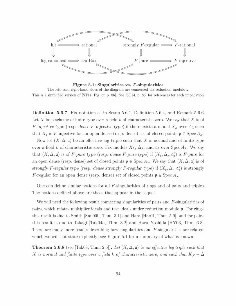
klt rational strongly F -regular F -rational

log canonical Du Bois F -pure F -injective

Figure 5.1: Singularities vs. F -singularitiesThe left- and right-hand sides of the diagram are connected via reduction modulo p.

This is a simplified version of [ST14, Fig. on p. 86]. See [ST14, p. 86] for references for each implication.

Definition 5.6.7. Fix notation as in Setup 5.6.1, Definition 5.6.4, and Remark 5.6.6.

Let X be a scheme of finite type over a field k of characteristic zero. We say that X is of

F -injective type (resp. dense F -injective type) if there exists a model Xλ over Aλ such

that Xp is F -injective for an open dense (resp. dense) set of closed points p ∈ SpecAλ.

Now let (X,∆, a) be an effective log triple such that X is normal and of finite type

over a field k of characteristic zero. Fix models Xλ, ∆λ, and aλ over SpecAλ. We say

that (X,∆, a) is of F -pure type (resp. dense F -pure type) if (Xp,∆p, atp) is F -pure for

an open dense (resp. dense) set of closed points p ∈ SpecAλ. We say that (X,∆, a) is of

strongly F -regular type (resp. dense strongly F -regular type) if (Xp,∆p, atp) is strongly

F -regular for an open dense (resp. dense) set of closed points p ∈ SpecAλ.

One can define similar notions for all F -singularities of rings and of pairs and triples.

The notions defined above are those that appear in the sequel.

We will need the following result connecting singularities of pairs and F -singularities of

pairs, which relates multiplier ideals and test ideals under reduction modulo p. For rings,

this result is due to Smith [Smi00b, Thm. 3.1] and Hara [Har01, Thm. 5.9], and for pairs,

this result is due to Takagi [Tak04a, Thm. 3.2] and Hara–Yoshida [HY03, Thm. 6.8].

There are many more results describing how singularities and F -singularities are related,

which we will not state explicitly; see Figure 5.1 for a summary of what is known.

Theorem 5.6.8 (see [Tak08, Thm. 2.5]). Let (X,∆, a) be an effective log triple such that

X is normal and finite type over a field k of characteristic zero, and such that KX + ∆

94

is R-Cartier. With notation as in Setup 5.6.1, Definition 5.6.4, and Remark 5.6.6, fix

models Xλ, ∆λ, and aλ over SpecAλ. Then, for all t ≥ 0, we have

J((X,∆); at

)p

= τ((Xp,∆p); a

tp

)(5.16)

when charκ(p) is sufficiently large. In particular, (X,∆, at) is klt if and only if (X,∆, at)

is of strongly F -regular type. Moreover, for every sequence of closed points p ∈ SpecAλ

such that the characteristic of κ(p) goes to infinity, we have that the limit of the F -pure

thresholds fptx((Xp,∆p); ap) is the log canonical threshold lctx((X,∆); a).

Note that implicit in the statement of Theorem 5.6.8 is that both objects in (5.16) make

sense. For the left-hand side, this requires choosing a model of a log resolution as well,

from which one obtains a model of J ((X,∆); at). We also note that the characteristic of

κ(p) is unbounded by Lemma 5.6.5.

Proof. All but the last part of the statement of Theorem 5.6.8 is proved in [Tak08, Thm.

2.5]. To prove this last statement, let pii∈N be a sequence of closed points in SpecAλ

such that charκ(pi)→∞ as i→∞. We claim that for every s ≥ 0, we have

lctx((X,∆); a

)≥ fptx

((Xpi ,∆pi); api

)> s (5.17)

for i 0. The first inequality automatically holds since the inclusion ⊇ in (5.16) holds

for every p ∈ SpecAλ; see [Sch10b, Thm. 6.7]. The second inequality holds for i 0

since (5.16) holds for s = t when charκ(pi) is sufficiently large.

95

Chapter 6

The ampleness criterion of

de Fernex–Kuronya–Lazarsfeld

In this chapter, we prove a criterion for ampleness using asymptotic cohomological

functions (Theorem E), which is originally due to de Fernex, Kuronya, and Lazarsfeld

over the complex numbers [dFKL07, Thm. 4.1]. A key ingredient is a lemma asserting

that the base ideals associated to multiples of a non-nef divisor grow at least like powers

of an ideal defining a curve (Proposition 6.2.1). This material is mostly from [Mur], with

some modifications in the proof of Proposition 6.2.1 using ideas from [MPST, Lems. 4.3

and 4.4].

We briefly describe the main difficulties in adapting the proof of [dFKL07, Thm. 4.1]

to positive characteristic. First, the proof of [dFKL07, Prop. 3.1] requires resolutions of

singularities, and because of this, we need to adapt the proof to use alterations instead.

Second, we need to replace asymptotic multiplier ideals with asymptotic test ideals in

the same proof, which requires reducing to the case when the ground field is F -finite by

using the gamma construction (Theorem B.1.1). Finally, [dFKL07] uses the assumption

that the ground field is uncountable to choose countably many very general divisors that

facilitate an inductive argument. Our version of [dFKL07, Thm. 4.1] therefore needs to

reduce to this case.

96

6.1. Motivation and statement

We start by motivating the statement of our ampleness criterion. Let X be a projective

variety of dimension n > 0. For every Cartier divisor L on X, we have

hi(X,OX(mL)

)= O(mn)

for every i; see [Laz04a, Ex. 1.2.20]. In [dFKL07, Thm. 4.1], de Fernex, Kuronya, and

Lazarsfeld asked when the higher cohomology groups have submaximal growth, i.e., when

hi(X,OX(mL)

)= o(mn).

They proved that over the complex numbers, ample Cartier divisors L are characterized

by having submaximal growth of higher cohomology groups for small perturbations of L.

We prove the following version of their result, which is valid over arbitrary fields, and

in particular, is valid over possibly imperfect fields of positive characteristic.

Theorem E. Let X be a projective variety of dimension n > 0 over a field k. Let L be

an R-Cartier divisor on X, and consider the following property:

(?) There exists a very ample Cartier divisor A on X and a real number ε > 0 such

that

hi(X,L− tA) := lim supm→∞

hi(X,OX

(dm(L− tA)e

))

mn/n!= 0

for all i > 0 and for all t ∈ [0, ε).

Then, L is ample if and only if L satisfies (?) for some pair (A, ε).

We note that one can have hi(X,L) = 0 for all i > 0 without L being ample, or even

pseudoeffective, as seen in the following example.

Example 6.1.1 [Kur06, Ex. 3.3]. Let A be a abelian variety of dimension g over an

algebraically closed field k, and let L be a line bundle on A. We recall that K(L) ⊆ A is

defined to be the maximal closed subscheme of A such that the Mumford bundle

Λ(L) := m∗(L)⊗ p∗1(L)−1 ⊗ p∗2(L)−1

97

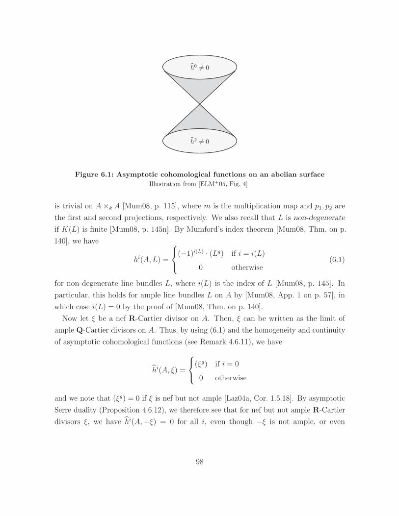
h0 6= 0

h2 6= 0

Figure 6.1: Asymptotic cohomological functions on an abelian surface

Illustration from [ELM+05, Fig. 4]

is trivial on A×k A [Mum08, p. 115], where m is the multiplication map and p1, p2 are

the first and second projections, respectively. We also recall that L is non-degenerate

if K(L) is finite [Mum08, p. 145n]. By Mumford’s index theorem [Mum08, Thm. on p.

140], we have

hi(A,L) =

(−1)i(L) · (Lg) if i = i(L)

0 otherwise(6.1)

for non-degenerate line bundles L, where i(L) is the index of L [Mum08, p. 145]. In

particular, this holds for ample line bundles L on A by [Mum08, App. 1 on p. 57], in

which case i(L) = 0 by the proof of [Mum08, Thm. on p. 140].

Now let ξ be a nef R-Cartier divisor on A. Then, ξ can be written as the limit of

ample Q-Cartier divisors on A. Thus, by using (6.1) and the homogeneity and continuity

of asymptotic cohomological functions (see Remark 4.6.11), we have

hi(A, ξ) =

(ξg) if i = 0

0 otherwise

and we note that (ξg) = 0 if ξ is nef but not ample [Laz04a, Cor. 1.5.18]. By asymptotic

Serre duality (Proposition 4.6.12), we therefore see that for nef but not ample R-Cartier

divisors ξ, we have hi(A,−ξ) = 0 for all i, even though −ξ is not ample, or even

98

pseudoeffective.

We now illustrate this phenomenon in a more concrete situation. Recall that if X is a

complete scheme over a field, then the Neron–Severi space is the R-vector space

N1R(X) := CartR(X)/≡R, (6.2)

where ≡R denotes R-linear equivalence. This vector space is finite-dimensional by

[Cut15, Prop. 2.3]. Now if A is an abelian surface, then the ample cone in N1R(X) is

ξ ∈ N1R(X) | h0(ξ) 6= 0. By [Laz04a, Lem. 1.5.4], the classes −ξ considered above for

nef but not ample R-Cartier divisors ξ correspond to classes in the boundary of the cone

ξ ∈ N1R(X) | h2(ξ) 6= 0. See Figure 6.1 for an illustration of the case when the Picard

rank ρ(A) of A is 3. We note that if A = E ×k E for a sufficiently general elliptic curve

E, then ρ(A) = 3. This follows from the fact that Endk(E)⊗Z Q ' Q for sufficiently

general E by a theorem of Deuring [Mum08, Thm. on p. 201], hence ρ(A) = 3 by a

lemma of Murty [Laf, Prop. 2.3].

6.2. A lemma on base loci

A key ingredient in our proof of Theorem E is the following result on base loci, which is

the analogue of [dFKL07, Prop. 3.1] over arbitrary fields. The lemma says that base

ideals associated to multiples of non-nef divisors grow like powers of an ideal defining a

curve.

Proposition 6.2.1. Let V be a normal projective variety of dimension at least two over

a field k. Let D be a Cartier divisor on V , and suppose there exists an integral curve

Z ⊆ V such that (D ·Z) < 0. Denoting by a ⊆ OV the ideal sheaf defining Z, there exist

positive integers q and c such that for every integer m ≥ c, we have

b(|mqD|

)⊆ am−c.

Here, b(|D|) denotes the base ideal of the Cartier divisor D; see Definition 4.5.1.

To use Bertini theorems, we need to reduce to the case when the ground field k is

infinite. Moreover, in positive characteristic, we use asymptotic test ideals instead of

asymptotic multiplier ideals, which requires also reducing to the case where the ground

99

field is F -finite.

Lemma 6.2.2. To prove Proposition 6.2.1, we may assume that the ground field k is

infinite, and in positive characteristic, we may also assume that k is F -finite.

Proof. We first construct a sequence k ⊆ k′ ⊆ K of two field extensions such that V ×kKis integral and normal, where k′ is infinite and K is F -finite in positive characteristic.

If k is already infinite, then let k′ = k. Otherwise, consider the purely transcendental

extension k ⊆ k(x). To show that V ×k k′ is integral and normal, let⋃j Uj be an

affine open covering of V . Then, V ×k k′ is covered by affine open subsets that are

localizations of the normal varieties Uj ×k Spec k[x], which pairwise intersect, hence

V ×k k′ is integral and normal. The same argument shows that Z ×k k′ is an integral

curve. We set K = k′ in characteristic zero, and in positive characteristic, the gamma

construction (Theorem B.1.6) shows that there is a field extension k′ ⊆ K such that

K is F -finite, V ×k K is integral and normal, and Z ×k K is integral. Note that K is

infinite since it contains the infinite field k′.

We now show that the special case when k is infinite and F -finite implies the general

case. Let π : V ×k k′ → V be the first projection morphism, which we note is faithfully

flat by base change. Since (π∗D · π∗Z) = (D · Z) < 0 by [Kle05, Prop. B.17], the special

case of Proposition 6.2.1 implies

b(|mq π∗D|

)⊆ (π−1a · OV×kk′)m−c.

Then, since π is faithfully flat and since b(|mq π∗D|) = π−1b(|mqD|) · OV×kk′ by flat

base change, we have b(|mqD|) ⊆ am−c by [Mat89, Thm. 7.5(ii)].

Remark 6.2.3. When k is F -finite of characteristic p > 0, then one can set K to be

k(x1/p∞) in the proof of Lemma 6.2.2, since integrality and normality are preserved under

limits of schemes with affine and flat transition morphisms [EGAIV2, Cor. 5.13.4].

We now focus on proving Proposition 6.2.1 in positive characteristic; see Remark 6.2.4

for the characteristic zero case. We have incorporated some ideas from [MPST, Lems.

4.3 and 4.4]. In the proof below, we will use the fact [Kle05, Lem. B.12] that if W is a

one-dimensional subscheme of a complete scheme X over a field, and if D is a Cartier

100

divisor on X, then

(D ·W ) =∑

α

lengthOX,ηα(OWα,ηα

)· (D ·Wα), (6.3)

where the Wα are the one-dimensional components of W with generic points ηα ∈ Wα.

Proof of Proposition 6.2.1 in positive characteristic. By Lemma 6.2.2, it suffices to con-

sider the case when the ground field k is infinite and F -finite. The statement is trivial

if H0(V,OV (mD)) = 0 for every integer m > 0, since in this case b(|mqD|) = 0 for all

positive integers m, q. We therefore assume H0(V,OV (mD)) 6= 0 for some integer m > 0.

We first set some notation. Let η : V1 → V be the normalized blowup of Z ⊆ V , and

denote E := η−1(Z). Consider a regular alteration ϕ : V ′ → V1 for (V1, E) as in [dJ96,

Thm. 4.1], and set D′ := (η ϕ)∗D. Note that in this case, E ′ := ϕ∗E = (η ϕ)−1(Z) is

a Cartier divisor with simple normal crossing support. The proof proceeds in four steps.

Step 1. It suffices to show that there exists a positive integer a such that for every

integer m > 0, we have

b(|maD′|

)⊆ OV ′(−mE ′red). (6.4)

Consider the commutative diagram

V ′ V2

V1 V

ϕ2

ϕϕ1

η

where the triangle is the Stein factorization for ϕ [Har77, Cor. III.11.5]. Note that by

construction of the Stein factorization, the scheme V2 is a normal projective variety. Now

by setting b to be the largest coefficient appearing in E ′, we see that OV ′(−bEred) ⊆OV ′(−E). Thus, we have

ϕ−12 b(|mab (η ϕ1)∗D|

)· OV ′ = b

(|mabD′|

)⊆ OV ′(−mbE ′red) ⊆ OV ′(−mE ′) (6.5)

by (6.4), where the first equality holds by Lemma 4.5.2 since ϕ2 is birational. Setting

101

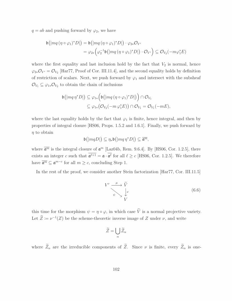
q = ab and pushing forward by ϕ2, we have

b(|mq (η ϕ1)∗D|

)= b(|mq (η ϕ1)∗D|

)· ϕ2∗OV ′

= ϕ2∗(ϕ−1

2 b(|mq (η ϕ1)∗D|

)· OV ′

)⊆ OV2(−mϕ∗1E)

where the first equality and last inclusion hold by the fact that V2 is normal, hence

ϕ2∗OV ′ = OV2 [Har77, Proof of Cor. III.11.4], and the second equality holds by definition

of restriction of scalars. Next, we push forward by ϕ1 and intersect with the subsheaf

OV1 ⊆ ϕ1∗OV2 to obtain the chain of inclusions

b(|mq η∗D|

)⊆ ϕ1∗

(b(|mq (η ϕ1)∗D|

))∩ OV1

⊆ ϕ1∗(OV2(−mϕ∗1E)

)∩ OV1 = OV1(−mE),

where the last equality holds by the fact that ϕ1 is finite, hence integral, and then by

properties of integral closure [HS06, Props. 1.5.2 and 1.6.1]. Finally, we push forward by

η to obtain

b(|mqD|

)⊆ η∗b

(|mq η∗D|

)⊆ am,

where am is the integral closure of am [Laz04b, Rem. 9.6.4]. By [HS06, Cor. 1.2.5], there

exists an integer c such that a`+1 = a · a` for all ` ≥ c [HS06, Cor. 1.2.5]. We therefore

have am ⊆ am−c for all m ≥ c, concluding Step 1.

In the rest of the proof, we consider another Stein factorization [Har77, Cor. III.11.5]

V ′ V

V

µ

ψν (6.6)

this time for the morphism ψ = η ϕ, in which case V is a normal projective variety.

Let Z := ν−1(Z) be the scheme-theoretic inverse image of Z under ν, and write

Z =⋃

α

Zα

where Zα are the irreducible components of Z. Since ν is finite, every Zα is one-

102

dimensional and dominates Z, hence the projection formula and (6.3) imply ν∗D · Zα < 0.

We also note that E ′ = µ−1(Z) is a Cartier divisor with simple normal crossing support

by the factorization (6.6).

We also fix the following notation. Fix a very ample Cartier divisor H on V ′, and set

A = KV ′ + (dimV ′+ 1)H. For every subvariety W ⊆ V ′, a complete intersection curve is

a curve formed by taking the intersection of dimW −1 hyperplane sections in∣∣H|W

∣∣, and

a general complete intersection curve is one formed by taking these hyperplane sections

to be general in∣∣H|W

∣∣. For each positive integer q, we will consider the asymptotic test

ideal

τ(V ′, ‖qD′‖

)= τ(‖qD′‖

)⊆ OV ′ .

By uniform global generation for test ideals (Theorem 5.5.13), the sheaf

τ(‖qD′‖

)⊗OV ′(qD′ + A) (6.7)

is globally generated for every integer q > 0.

Step 2. There exists an integer `0 > 0 such that for every integer ` > `0 and for every

irreducible component F of E ′red that dominates (Zα)red for some α, we have

τ(‖`D′‖

)⊆ OV ′(−F ).

Let C ⊆ F be a general complete intersection curve; note that C is integral by Bertini’s

theorem [FOV99, Thm. 3.4.10 and Cor. 3.4.14] and dominates (Zα)red for some α, hence

(D′ · C) < 0 by the projection formula and (6.3). If for some integer q > 0, the curve

C is not contained in the zero locus of τ(‖qD′‖), then the fact that the sheaf (6.7) is

globally generated implies ((qD′ + A) · C

)≥ 0.

Letting `0F = −(A ·C)/(D′ ·C), we see that the ideal τ(‖`D′‖) vanishes everywhere along

C for every integer ` > `0F . By varying C, the ideal τ(‖`D′‖) must vanish everywhere

along F for every integer ` > `0F , hence we can set `0 = maxF`0F.Step 3. Let E ′i be an irreducible component of E ′red not dominating Zα for every α.

Suppose E ′j is another irreducible component of E ′red such that E ′i ∩E ′j 6= ∅ and for which

103

there exists an integer `j such that for every integer ` > `j, we have

τ(‖`D′‖

)⊆ OV ′(−E ′j).

Then, there is an integer `i ≥ `j such that for every integer ` > `i, we have

τ(‖`D′‖

)⊆ OV ′(−E ′i).

Let C ⊆ E ′i be a complete intersection curve. By the assumption that E ′ has simple

normal crossing support, there exists at least one closed point P ∈ C ∩ E ′j. For every

` > `j and every m > 0, we have the sequence of inclusions

(τ(‖m`D′‖

)⊗OV ′(m`D′ + A)

)· OC ⊆

(τ(‖`D′‖

)m ⊗OV ′(m`D′ + A))· OC

⊆(OV ′(−mE ′j)⊗OV ′(m`D′ + A)

)· OC ⊆ OC(A|C −mP )

(6.8)

where the first two inclusions follow from subadditivity (Theorem 5.5.8) and by assump-

tion, respectively. The last inclusion holds since C maps to a closed point in V , hence

OC(D′) = OC . By the global generation of the sheaf in (6.7) for q = m`, the inclusion

(6.8) implies that for every integer ` > `j , if τ(‖m`D′‖) does not vanish everywhere along

C, then (A · C) ≥ m. Choosing `i = `j · ((A · C) + 1), we see that τ(‖`D′‖) vanishes

everywhere along C for every integer ` > `i. By varying C, we have τ(‖`D′‖) ⊆ OV ′(−E ′i)for every integer ` > `i.

Step 4. There exists a positive integer a such that for every integer m > 0, we have

b(|maD′|) ⊆ OV ′(−mE ′red).

Write

E ′red =⋃

j

⋃

i∈IjE ′ij,

where the E ′ij are the irreducible components of E ′red, and the⋃i∈Ij E

′ij are the connected

components of E ′red. Since V is normal, each preimage µ−1(Zα) is connected by Zariski’s

main theorem [Har77, Cor. III.11.4], hence each connected component⋃i∈Ij E

′ij of E ′red

contains an irreducible component E ′i0j that dominates (Zα)red for some α. By Step 2,

there exists an integer `0 such that for every j, we have τ(‖`D′‖) ⊆ OV ′(−E ′i0j) for every

integer ` > `0. For each j, by applying Step 3 (|Ij| − 1) times to the jth connected

104

component⋃i∈Ij E

′ij of E ′, we can find `j such that τ(‖`D′‖) ⊆ OV ′(−E ′ij) for every i ∈ Ij

and for every integer ` > `j . Setting a = maxj`j+ 1, we have τ(‖aD′‖) ⊆ OV ′(−E ′red).

Thus, for every integer m > 0, we have

b(|maD′|

)⊆ τ

(|maD′|

)⊆ τ

(‖maD′‖

)⊆ τ

(‖aD′‖

)m ⊆ OV ′(−mE ′red),

where the first inclusion follows by the fact that V ′ is regular hence strongly F -regular

(Propositions 5.5.7(i) and 5.5.7(vii)), the second inclusion is by definition of the asymp-

totic test ideal, and the third inclusion is by subadditivity (Theorem 5.5.8). This

concludes the proof of Step 4, hence also of Proposition 6.2.1 by Step 1.

Remark 6.2.4. When char k = 0, it suffices to replace asymptotic test ideals in the

proof above with asymptotic multipliers ideals J (‖D‖) as defined in Definition 4.9.2 by

replacing Proposition 5.5.7, Theorem 5.5.8, and Theorem 5.5.13 with [dFM09, Prop. 2.3],

[JM12, Thm. A.2], and Theorem 4.9.4, respectively.

6.3. Proof of Theorem E

We now prove Theorem E. We first note that the direction ⇒ in Theorem E follows from

existing results.

Proof of ⇒ in Theorem E. Let A be a very ample Cartier divisor. Then, for all t such

that L− tA is ample, we have hi(X,L− tA) = 0 by Serre vanishing and by homogeneity

and continuity (see Remark 4.6.11).

For the direction ⇐, it suffices to show Theorem E for Cartier divisors L by continuity

and homogeneity (see Remark 4.6.11). We also make the following two reductions. Recall

that an R-Cartier divisor L on X satisfies (?) for a pair (A, ε) consisting of a very ample

Cartier divisor A on X and a real number ε > 0 if hi(X,L− tA) = 0 for all i > 0 and

all t ∈ [0, ε).

Lemma 6.3.1. To prove the direction ⇐ in Theorem E, we may assume that the ground

field k is uncountable.

105

Proof. Consider the purely transcendental extension

k′ := k(xα)α∈A

where xαα∈A is an uncountable set of indeterminates; note that k′ is uncountable by

construction. We claim that X ×k k′ is integral. Let⋃j Uj be an affine open covering of

X. Then, X ×k k′ is covered by affine open subsets that are localizations of the integral

varieties Uj ×k Spec k[xα]α∈A, which pairwise intersect, hence X ×k k′ is integral.

Now suppose X is a projective variety over k, and let L be an Cartier divisor satisfying

(?) for some pair (A, ε). Let

π : X ×k k′ −→ X

be the first projection map, which we note is faithfully flat by base change. Then, the

pullback π∗A of A is very ample, and to show that L is ample, it suffices to show that

π∗L is ample by flat base change and Serre’s criterion for ampleness. By the special case

of Theorem E over the ground field k′, it therefore suffices to show that π∗L satisfies (?)

for the pair (π∗A, ε).

We want to show that for every i > 0 and for all t ∈ [0, ε), we have

hi(X,L− tA) = hi(X ×k K, π∗(L− tA)

)= 0. (6.9)

For every D ∈ Cart(X) and every i ≥ 0, the number hi(X,OX(D)) is invariant under

ground field extensions by flat base change, hence hi(X,D) is also. By homogeneity and

continuity (see Remark 4.6.11), the number hi(X,D) is also invariant under ground field

extensions for D ∈ CartR(X), hence (6.9) holds.

Lemma 6.3.2. To prove the direction ⇐ in Theorem E, it suffices to show that every

Cartier divisor satisfying (?) is nef.

Proof. Suppose L is a Cartier divisor satisfying (?) for a pair (A, ε). Choose δ ∈ (0, ε)∩Q

and let m be a positive integer such that mδ is an integer. Then, the Cartier divisor

m(L− δA) is nef since

hi(X,m(L− δA)− tA

)= hi

(X,mL− (t+mδ)A

)

= m · hi(X,L−

( tm

+ δ)A)

= 0

106

for all t ∈ [0,mε − δ) by homogeneity (Proposition 4.6.9). Thus, the Cartier divisor

L = (L− δA) + δA is ample by [Laz04a, Cor. 1.4.10].

We will also need the following result to allow for an inductive proof. Note that the

proof in [dFKL07] works in our setting.

Lemma 6.3.3 [dFKL07, Lem. 4.3]. Let X be a projective variety of dimension n > 0

over an uncountable field, and let L be a Cartier divisor on X. Suppose L satisfies (?)

for a pair (A, ε), and let E ∈ |A| be a very general divisor. Then, the restriction L|Esatisfies (?) for the pair (A|E, ε).

We can now show the direction ⇐ in Theorem E; by Lemma 6.3.2, we need to show

that every Cartier divisor satisfying (?) is nef. Recall that by Lemma 6.3.1, we may

assume that the ground field k is uncountable. Our proof follows that in [dFKL07, pp.

450–454] after reducing to a setting where Proposition 6.2.1 applies, although we have to

be more careful in positive characteristic.

Proof of ⇐ in Theorem E. We proceed by induction on dimX. Suppose dimX = 1; we

will show the contrapositive. If L is not nef, then degL < 0 and −L is ample. Thus, by

asymptotic Serre duality (Proposition 4.6.12), we have h1(X,L) = h0(X,−L) 6= 0, hence

(?) does not hold for every choice of (A, ε).

We now assume dimX ≥ 2. Suppose by way of contradiction that there is a non-nef

Cartier divisor L satisfying (?), and let Z ⊆ X be an integral curve such that (L ·Z) < 0.

Our goal is to show that

h1(X,L− δA) 6= 0 (6.10)

for 0 < δ 1, contradicting (?). Let F ∈ |A| be a very general divisor. By Bertini’s

theorem [FOV99, Thm. 3.4.10 and Cor. 3.4.14], we may assume that F is a subvariety

of X, in which case by inductive hypothesis and Lemma 6.3.3, we have that L|F is

ample. Since ampleness is an open condition in families [EGAIV3, Cor. 9.6.4], there

exists an integer b > 0 such that bL is very ample along the generic divisor Fη ∈ |A|.By possibly replacing b with a multiple, we may also assume that mbL|Fη has vanishing

higher cohomology for every integer m > 0. Since the ground field k is uncountable, we

can then choose a sequence of very general Cartier divisors Eβ∞β=1 ⊆ |A| such that the

following properties hold:

107

(a) Eβ is a subvariety of X for all β (by Bertini’s theorem [FOV99, Thm. 3.4.10 and

Cor. 3.4.14]);

(b) For all β, bL|Eβ is very ample and mbL|Eβ has vanishing higher cohomology for

every integer m > 0 (by the constructibility of very ampleness in families [EGAIV3,

Prop. 9.6.3] and by semicontinuity); and

(c) For every positive integer r, the k-dimension of cohomology groups of the form

Hj(Eβ1 ∩ Eβ2 ∩ · · · ∩ Eβr ,OEβ1

∩Eβ2∩···∩Eβr (mL)

)(6.11)

for non-negative integers j and m is independent of the r-tuple (β1, β2, . . . , βr) (by

semicontinuity; see [Kur06, Prop. 5.5]).

We will denote by hj(OE1∩E2∩···∩Er(mL)) the dimensions of the cohomology groups (6.11).

By homogeneity (Proposition 4.6.9), we can replace L by bL so that L|Eβ is very ample

with vanishing higher cohomology for all β.

To show (6.10), we now follow the proof in [dFKL07, pp. 453–454] with appropriate

modifications. Given positive integers m and r, consider the complex

K•m,r :=

( r⊗

β=1

(OX −→ OEβ

))⊗OX(mL)

=

OX(mL) −→

r⊕

β=1

OEβ(mL) −→⊕

1≤β1<β2≤rOEβ1

∩Eβ2(mL) −→ · · ·

.

By [Kur06, Cor. 4.2], this complex is acyclic away from OX(mL), hence is a resolution

for OX(mL− rA). In particular, we have

Hj(X,OX(mL− rA)

)= Hj(X,K•m,r).

The right-hand side is computed by an E1-spectral sequence whose first page is shown in

Figure 6.2. This spectral sequence yields a natural inclusion

ker(um,r)

im(vm,r)⊆ H1

(X,OX(mL− rA)

). (6.12)

We want to bound the left-hand side of (6.12) from below. First, there exists a constant

108

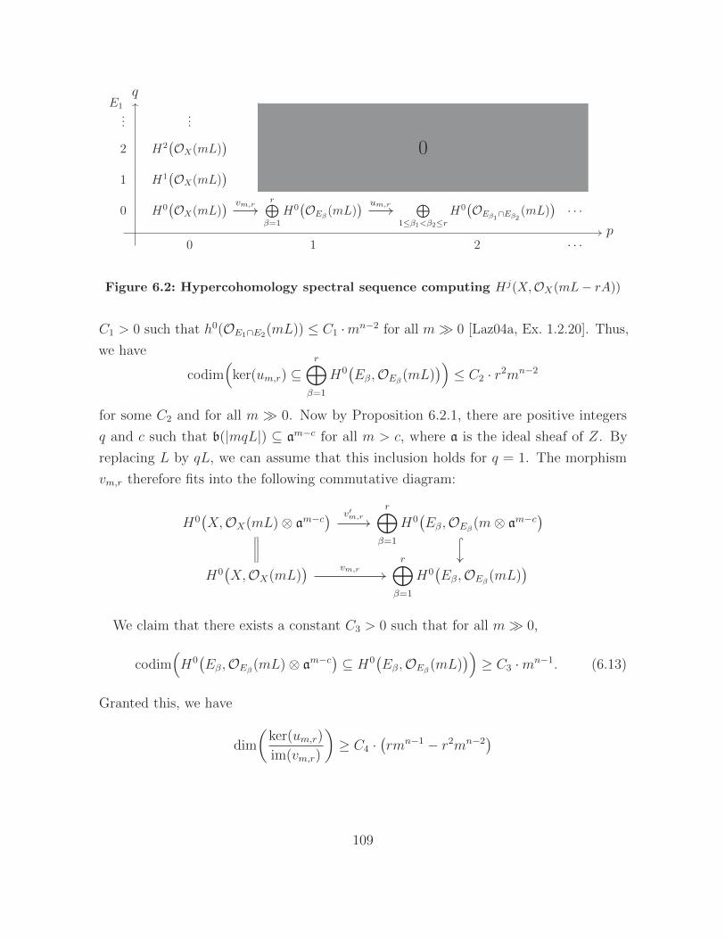
E1...

...

2 H2(OX(mL)

)

1 H1(OX(mL)

)

0 H0(OX(mL)

) r⊕β=1

H0(OEβ(mL)

) ⊕1≤β1<β2≤r

H0(OEβ1∩Eβ2 (mL)

)· · ·

0 1 2 · · ·

q

p

0

vm,r um,r

Figure 6.2: Hypercohomology spectral sequence computing Hj(X,OX(mL− rA))

C1 > 0 such that h0(OE1∩E2(mL)) ≤ C1 ·mn−2 for all m 0 [Laz04a, Ex. 1.2.20]. Thus,

we have

codim(

ker(um,r) ⊆r⊕

β=1

H0(Eβ,OEβ(mL)

))≤ C2 · r2mn−2

for some C2 and for all m 0. Now by Proposition 6.2.1, there are positive integers

q and c such that b(|mqL|) ⊆ am−c for all m > c, where a is the ideal sheaf of Z. By

replacing L by qL, we can assume that this inclusion holds for q = 1. The morphism

vm,r therefore fits into the following commutative diagram:

H0(X,OX(mL)⊗ am−c

) r⊕

β=1

H0(Eβ,OEβ(m⊗ am−c

)

H0(X,OX(mL)

) r⊕

β=1

H0(Eβ,OEβ(mL)

)

v′m,r

vm,r

We claim that there exists a constant C3 > 0 such that for all m 0,

codim(H0(Eβ,OEβ(mL)⊗ am−c

)⊆ H0

(Eβ,OEβ(mL)

))≥ C3 ·mn−1. (6.13)

Granted this, we have

dim

(ker(um,r)

im(vm,r)

)≥ C4 ·

(rmn−1 − r2mn−2

)

109

for some constant C4 > 0 and for all m 0. Fixing a rational number 0 < δ 1 and

setting r = mδ for an integer m > 0 such that mδ is an integer, we then see that there

exists a constant C5 > 0 such that

h1(X,OX

(m(L− δA)

))≥ C5 · δmn

for all m 0, contradicting (?).

It remains to show (6.13). Since the vanishing locus of a may have no k-rational points,

we will pass to the algebraic closure of k to bound the codimension on the left-hand side

of (6.13) from below. Let Eβ := Eβ ×k k, and denote by π : Eβ → Eβ the projection

morphism. Note that

codim(H0(Eβ,OEβ(mL)⊗ am−c

)⊆ H0

(Eβ,OEβ(mL)

))

= codim(H0(Eβ,OEβ(mπ∗L)⊗ π−1am−c · OEβ

)⊆ H0

(Eβ,OEβ(mπ∗L)

))

by the flatness of k ⊆ k. Since OEβ(π∗L) is very ample by base change, we can choose a

closed point x ∈ Z(π−1a · OEβ) ∩ Eβ, in which case OEβ(mπ∗L) separates (m− c)-jets

at x by [Ito13, Proof of Lem. 3.7] (see also Lemma 7.2.5). Finally, the dimension of the

space of (m− c)-jets at x is at least that for a regular point of a variety of dimension n,

hence

codim(H0(Eβ,OEβ(mπ∗L)⊗ π−1am−c · OEβ

)⊆ H0

(Eβ,OEβ(mπ∗L)

))

≥ codim(H0(Eβ,OEβ(mπ∗L)⊗mm−c

x · OEβ)⊆ H0

(Eβ,OEβ(mπ∗L)

))

≥(m− c+ n

n− 1

)≥ C3 ·mn−1

for some constant C3 > 0 and all m 0, as required.

110

Chapter 7

Moving Seshadri constants

Moving Seshadri constants were defined by Nakamaye [Nak03] as a generalization of the

Seshadri constant introduced in §2.2 to arbitrary R-Cartier divisors. In this chapter, we

extend basic results on moving Seshadri constants from [Nak03; ELM+09, §6] to the

setting of possibly singular varieties over arbitrary fields. These results are new even for

complex projective varieties that are not smooth. Some of this material will appear in

joint work with Mihai Fulger [FMb].

7.1. Definition and basic properties

Following [ELM+09], we define the moving Seshadri constant as follows:

Definition 7.1.1 (cf. [ELM+09, Def. 6.1]). Let X be a normal projective variety over a

field k and let D be an R-Cartier divisor on X. Consider a k-rational point x ∈ X. If

x /∈ B+(D), then the moving Seshadri constant of D at x is

ε(‖D‖;x

):= sup

f∗D≡RA+Eε(A;x) (7.1)

where the supremum runs over all birational morphisms f : X ′ → X from normal

projective varieties X ′ that are isomorphisms over a neighborhood of x, and R-numerical

equivalences f ∗D ≡R A+E where A is an ample R-Cartier divisor and E is an effective

R-Cartier divisor such that x /∈ f(Supp(E)). If x ∈ B+(D), then we set ε(‖D‖;x) = 0.

By definition, x ∈ B+(D) if and only if ε(‖D‖;x) = 0.

111

Note that R-numerical equivalences of the form in (7.1) exist since f−1(x) /∈ B+(f ∗D)

by Proposition 4.6.4.

We collect some elementary properties of moving Seshadri constants. Recall that if

x ∈ X is a closed point, then BigxR (X) denotes the open convex subcone of the big cone

consisting of big R-Cartier divisor classes D ∈ N1R(X) such that x /∈ B+(D) [ELM+09,

Def. 5.1]. Here N1R(X) is the Neron–Severi space associated to X defined in (6.2).

Proposition 7.1.2 (cf. [ELM+09, Prop. 6.3 and Rem. 6.5]). Let X be a normal projective

variety over a field k and let x ∈ X be a k-rational point. Then, the function

BigxR (X) R>0

D ε(‖D‖;x

)

is continuous. Moreover, if D is an R-Cartier divisor, then we have the following:

(i) ε(‖D‖;x) ≤ (volX(D)/e(OX,x))1/ dimX .

(ii) If D and E are numerically equivalent R-Cartier divisors, then ε(‖D‖;x) =

ε(‖E‖;x).

(iii) ε(‖λD‖;x) = λ · ε(‖D‖;x) for every positive real number λ.

(iv) If D′ is another R-Cartier divisor such that x /∈ B+(D) ∪B+(D′), then

ε(‖D +D′‖;x) ≥ ε

(‖D‖;x

)+ ε(‖D′‖;x

).

(v) If D is a nef R-Cartier divisor, then ε(‖D‖;x) = ε(D;x).

Proof. (i)–(iv) follow by definition and from the analogous properties for usual Seshadri

constants; for (i), the analogous property is [Laz04a, Prop. 5.1.9]. The continuity property

follows from (iii) and (iv) by [ELM+09, Rem. 5.4].

We now prove (v), following [ELM+09, Rem. 6.5]. If x ∈ B+(D), then ε(‖D‖;x) = 0

by definition, while ε(D;x) = 0 by combining Theorem 4.6.6 and [Laz04a, Prop. 5.1.9].

It therefore suffices to consider the case when x /∈ B+(D). As in Definition 7.1.1, choose

a birational morphism f : X ′ → X with a decomposition f ∗D ≡R A+ E. We have

ε(D;x) = ε(f ∗D; f−1(x)

)≥ ε(A; f−1(x)

)

112

where the first equality holds since D is nef and f is an isomorphism at x. The second

inequality holds by combining (2.3) and the fact that x /∈ f(Supp(E)), hence E · C ≥ 0

for every integral curve C ⊆ X ′ passing through f−1(x). Taking the supremum over all

f as in Definition 7.1.1, we have the inequality ε(D;x) ≥ ε(‖D‖;x). For the opposite

inequality, write D ≡R A + E with A an ample R-Cartier divisor and E an effective

R-Cartier divisor not containing x in its support. For every integer n ≥ 1, we can write

D ≡R1

nA+

n− 1

nD +

1

nE,

hence setting An := 1nA+ n−1

nD, we have D ≡R An + 1

nE for an ample R-Cartier divisor

An and a fixed effective R-Cartier divisor E. We therefore have

ε(‖D‖;x

)≥ ε(An;x) (7.2)

for all n. Now we note that using the characterization in (2.3), we have

ε(An;x) = infC3x

(An · C)

e(OC,x)

≥ inf

C3x

(D · C)

e(OC,x)

+

1

ninfC3x

(−E · C)

e(OC,x)

. (7.3)

Taking the limit n→∞ in (7.2), we obtain the inequality ε(‖D‖;x) ≥ ε(D;x).

Remark 7.1.3. We note that the continuity statement in Proposition 7.1.2 is not the

analogue of [ELM+09, Thm. 6.2], which states that if X is a smooth complex projective

variety and x ∈ X is a closed point, then the function D 7→ ε(‖D‖;x) is continuous on

the entire Neron–Severi space N1R(X). A proof of this statement would require extending

the main results about restricted volume functions in [ELM+09] to our setting.

7.2. Alternative descriptions

We now give alternative characterizations of the moving Seshadri constant defined in

Definition 7.1.1.

113

7.2.1. Nakamaye’s description

Moving Seshadri constants were first defined by Nakamaye by decomposing the complete

linear system |D| into its moving and fixed parts on a birational model of X. The

following is a version of his definition that works over arbitrary fields.

Definition 7.2.1 (cf. [Nak03, Def. 0.4]). Let X be a normal projective variety over a

field k and let D be a Q-Cartier divisor on X. Let x /∈ B(D) be a k-rational point.

For every integer m ≥ 1 such that mD is Cartier and x /∈ Bs(|mD|), let πm : Xm → X

be a morphism from a normal projective variety Xm that is an isomorphism over a

neighborhood of x, and such that π−1m b(|mD|) ·OXm = OXm(−Fm) for an effective Cartier

divisor Fm. We can then write

∣∣π∗m(mD)∣∣ = |Mm|+ Fm,

where |Mm| is the moving part and Fm is the fixed part of the linear system |π∗m(mD)|,respectively. We then set

εN(‖D‖;x

):= lim sup

m→∞

ε(Mm; π−1

m (x))

m

where the limit supremum is taken over all m such that mD is integral.

To make sure that εN(‖D‖;x) is well-defined, we show that ε(Mm;π−1m (x)) does not

depend on the choice of morphism πm. First, any two morphisms πm : Xm → X and

π′m : X ′m → X as above can be dominated by a morphism π′′m : X ′′m → X satisfying

the same properties, and the normality of the varieties X,Xm, X′m, X

′′m imply that the

moving parts on Xm and X ′m pullback to the moving part on X ′′m. Since πm, π′m, π

′′m

are all isomorphisms in a neighborhood of x, we see that the Seshadri constants of

Mm,M′m,M

′′m are equal, hence ε(Mm; π−1

m (x)) does not depend on the choice of πm.

We now show that the limit supremum used to define εN(‖D‖;x) is equal to a limit.

Lemma 7.2.2. With notation as in Definition 7.2.1, we have

εN(‖D‖;x

)= lim

m→∞

ε(Mm; π−1

m (x))

m= sup

m

ε(Mm; π−1

m (x))

m.

114

Proof. Let m and n be positive integers such that mD and nD are Cartier divisors.

Choose π : X ′ → X that satisfies the properties in Definition 7.2.1 for |mD|, |nD|, and

|(m + n)D|, for example by blowup up the base loci for all three linear systems, and

then taking a normalization. Since we have Mm+n = Mm +Mn + E for some effective

divisor E with π−1(x) /∈ Supp(E), we deduce that

ε(Mm+n; π−1(x)

)≥ ε(Mm; π−1(x)

)+ ε(Mn; π−1(x)

).

Thus, the sequence ε(Mm; π−1m (x))m is superadditive, and Fekete’s lemma [PS98, Pt. I,

no 98] implies that the limit supremum is equal to the limit and the supremum.

Nakamaye’s definition coincides with the one in Definition 7.1.1 for x /∈ B(D).

Proposition 7.2.3 (cf. [ELM+09, Prop. 6.4]). Let X be a normal projective variety

over a field k and let D be a Q-Cartier divisor. If x /∈ B(D) is a k-rational point, then

ε(‖D‖;x) = εN(‖D‖;x).

Proof. By Proposition 7.1.2(iii) and Lemma 7.2.2, both invariants are homogeneous

with respect to taking integer multiples of D. It therefore suffices to consider the case

when D is integral, B(D) = Bs(|D|)red, and |D| induces a rational map birational onto

its image. Let m be a positive integer, and let πm : Xm → X be as in Definition 7.2.1.

Writing |π∗m(mD)| = |Mm| + Fm, we note that by assumption on x, we have that

π−1m (x) /∈ Supp(Fm).

First, suppose that x ∈ B+(D). By assumption, x /∈ B(D) = Bs(|D|)red, hence

π−1m (x) /∈ Bs(|π∗mD|)red = Supp(Fm) by the normality of X. Thus, Proposition 4.6.4

implies π−1m (x) ∈ B+(Mm), and Theorem 4.6.6 implies there exists a subvariety V ⊆ Xm

such that π−1m (x) ∈ V and (MdimV

m · V ) = 0. We therefore see that ε(Mm; π−1m (x)) = 0

by [Laz04a, Prop. 5.1.9]. Since this is true for every m, we have that εN(‖D‖;x) = 0,

hence ε(‖D‖;x) = εN(‖D‖;x) when x ∈ B+(D).

In the rest of the proof, we therefore assume that x /∈ B+(D). Since |Mm| induces

a map birational onto the image of X ′ by the assumption that |D| induces a rational

map birational onto its image, we may write Mm ≡Q A+ E, where A and E are ample

and effective Q-Cartier divisors, respectively, such that π−1m (x) /∈ Supp(E) [Laz04a, Cor.

115

2.2.7]. For every integer n ≥ 1, we can write

Mm ≡Q1

nA+

n− 1

nMm +

1

nE,

hence setting An := 1nA + n−1

nMm, we have Mm ≡Q An + 1

nE for an ample Q-Cartier

divisor An and a fixed effective Q-Cartier divisor E. By Definition 7.1.1, we see that

ε(‖D‖;x

)≥ ε

(An; π−1

m (x))

m

for every n. Using (7.3) and taking the limit as n→∞, we see that

ε(‖D‖;x

)≥ ε

(Mm; π−1

m (x))

m,

hence ε(‖D‖;x) ≥ εN(‖D‖;x).

We now show the reverse inequality. Let f : X ′ → X and f ∗D ≡R A + E be as in

Definition 7.1.1. Fix m such that mA is a very ample Cartier divisor. By taking a

normalized blowup of the base locus of f ∗(mD), which by assumption is an isomorphism

in a neighborhood of f−1(x), we can write

|f ∗(mD)| = |Mm|+ Fm

as in Definition 7.2.1. Since mA is free, we have Mm ∼ mA+ F ′m for an effective Cartier

divisor F ′m such that F ′m ≤ mE, hence f−1(x) /∈ Supp(F ′m). We therefore have

ε(Mm; π−1

m (x))

m≥ ε(A; f−1(x)

),

hence εN(‖D‖;x) ≥ ε(‖D‖;x).

7.2.2. A description in terms of jet separation

We now show that just as for usual Seshadri constants of ample Cartier divisors at regular

closed points on projective varieties [Laz04a, Thm. 5.1.17], moving Seshadri constants

can be described using separation of jets. Note that this description (Proposition 7.2.10)

is new even in characteristic zero for singular points.

116

Recall from Definition 2.2.4 that if X is a scheme, x ∈ X is a closed point, and ` ≥ −1

is an integer, a coherent sheaf F separates `-jets at x if the restriction morphism

H0(X,F ) −→ H0(X,F ⊗OX/m`+1x )

is surjective, and that we denote by s(F ;x) the largest integer ` ≥ −1 such that F

separates `-jets at x. We can then define moving Seshadri constants using jet separation.

Definition 7.2.4. Let X be a projective variety over a field k and let D be a Q-Cartier

divisor on X. Consider a k-rational point x ∈ X with defining ideal mx ⊆ OX . We set

εjet

(‖D‖;x

):= lim sup

m→∞

s(mD;x)

m,

where the limit supremum runs over all integers m ≥ 1 such that mD is integral.

We now prove that the limit supremum used to define εjet(‖D‖;x) is equal to a limit.

Lemma 7.2.5 ([FMa, Lem. 6.4]; cf. [Ito13, Proof of Lem. 3.7]). Let X be a scheme, and

let F and G be coherent sheaves on X. Then, for every closed point x ∈ X such that

s(F ;x) ≥ 0 and s(G ;x) ≥ 0, we have

s(F ;x) + s(G ;x) ≤ s(F ⊗ G ;x).

With notation in Definition 7.2.4, we therefore have

εjet

(‖D‖;x

)= lim

m→∞s(mD;x)

m= sup

m≥1

s(mD;x)

m.

Proof. We first show that a coherent sheaf F separates `-jets if and only if

H0(X,mixF ) −→ H0(X,mi

xF/mi+1x F ) (7.4)

is surjective for every i ∈ 0, 1, . . . , `. We proceed by induction on `. If ` = 0, then

there is nothing to show. Now suppose ` > 0. By induction and the fact that a coherent

sheaf separating `-jets also separates all lower order jets, it suffices to show that if F

separates (`− 1)-jets, then F separates `-jets if and only if (7.4) is surjective for i = `.

117

Consider the commutative diagram

0 m`xF F F/m`

xF 0

0 m`xF/m`+1

x F F/m`+1x F F/m`

xF 0

Taking global sections, we obtain the diagram

0 H0(X,m`xF ) H0(X,F ) H0(X,F/m`

xF ) 0

0 H0(X,m`xF/m`+1

x F ) H0(X,F/m`+1x F ) H0(X,F/m`

xF )

where the top row remains exact by the assumption that F separates (`− 1)-jets. By

the snake lemma, we see that the left vertical arrow is surjective if and only if the middle

vertical arrow is surjective, as desired.

We now prove the lemma. Suppose F separates i-jets and G separates j-jets. We

then have the commutative diagram

H0(X,mixF )⊗H0(X,mj

xG ) H0(X,mixF/mi+1

x F ⊗mjxG /m

j+1x G )

H0(X,mi+j

x (F ⊗ G ))

H0(X,mi+j

x (F ⊗ G )/mi+j+1x (F ⊗ G )

)

Since the top horizontal arrow is surjective by assumption, and the right vertical arrow

is surjective, essentially by the surjectivity of

mix/m

i+1x ⊗mj

x/mj+1x ' (mi

x ⊗mjx)⊗OX/mx mi+j

x /mi+j+1x ,

we see that the composition from the top left corner to the bottom right corner is surjective,

hence the bottom horizontal arrow is surjective. By running through all combinations of

integers i ≤ s(F ;x) and j ≤ s(G ;x), we see that s(F ;x) + s(G ;x) ≤ s(F ⊗ G ;x) by

the argument in the previous paragraph.

The last statement about εjet(‖D‖;x) follows from Fekete’s lemma [PS98, Pt. I, no 98],

since we have shown the superadditivity of the sequence s(mD;x)m≥1 provided that

118

x /∈ B(D). If x ∈ B(D), then s(mD;x) = −1 for all m ≥ 1 such that mD is integral,

hence the limit, limit supremum, and supremum are all equal to zero.

The constant εjet(‖D‖;x) detects B+(D).

Lemma 7.2.6. Let X be a normal projective variety over a field k and let D be a

Q-Cartier divisor on X. Consider a k-rational point x ∈ X. Then, x ∈ B+(D) if and

only if εjet(‖D‖;x) = 0.

Proof. For ⇐, note that εjet(‖D‖;x) = 0 implies s(mD;x) ≤ 0 for all m such that mD

is integral, since Lemma 7.2.5 implies εjet(‖D‖;x) is a supremum. If x ∈ B(D), then

x ∈ B+(D) as well, hence it suffices to consider the case when x /∈ B(D). Suppose

x /∈ B+(D), and let A be a very ample Cartier divisor on X. By [ELM+06, Prop. 1.5]

and [Laz04a, Prop. 2.1.21], there exist positive integers q, r such that

B+(D) = B(rD − A) = Bs(∣∣q(rD − A)

∣∣)red.

Since x /∈ B+(D), we see that |q(rD−A)| is basepoint-free at x. Moreover, since OX(qA)

separates 1-jets at x by the very ampleness of A, we see that OX(qrD) separates 1-jets

at x by Lemma 7.2.5, a contradiction.

For ⇒, we note that if x ∈ B(D), then s(mD;x) = −1 for all m such that mD

is integral, hence it suffices to consider the case when x ∈ B+(D) r B(D). Suppose

s(mD;x) > 0 for some integer m > 0. By possibly replacing m with a large and

divisible enough multiple, we may assume that B(mD) = Bs(|mD|)red by Lemma 7.2.5

and [Laz04a, Prop. 2.1.21]. Then, for every subvariety V ⊆ X containing x, we have

V 6⊆ Bs(|mD|)red. Moreover, since OX(mD) separates tangent directions at x, there

exists E ∈ |mD| not containing V , in which case (EdimV · V ) > 0.

Now let πm : Xm → X be the normalized blowup of b(|mD|), and write |π∗m(mD)| =|Mm|+ Fm where OXm(−Fm) = b(|mD|) · OXm . By Proposition 4.6.4 and the definition

of the augmented base locus, we have

π−1m (x) ∈ B+(π∗mD) ⊆ B+(Mm) ∪ Supp(Fm).

The fact that x /∈ B(D) implies π−1m (x) ∈ B+(Mm). By Theorem 4.6.6, there therefore

exists a subvariety W ⊆ Xm such that π−1m (x) ∈ W and (MdimW

m ·W ) = 0. Now choose

119

E ∈ |mD| as in the previous paragraph for V = πm∗W . Since Fm = (πm)−1 Bs(|mD|),we have that π∗mE − Fm is an effective Cartier divisor that contains π−1

m (x) but does not

contain W , hence

(MdimWm ·W ) =

((π∗mE − Fm)dimW ·W

)> 0,

a contradiction. We therefore have εjet(‖D‖;x) = 0 if x ∈ B+(D).

This lemma has the following consequence:

Corollary 7.2.7. Let X be a normal projective variety over an algebraically closed field k,

and let D be a Q-Cartier divisor on X. Then, D is ample if and only if εjet(‖D‖;x) > 0

for every closed point x ∈ X.

Proof. By Lemma 7.2.6, we have that εjet(‖D‖;x) > 0 for every closed point x ∈ X if

and only if B+(D) = ∅. This condition is equivalent to the ampleness of D by [ELM+06,

Ex. 1.7].

We now collect some properties of εjet(‖D‖;x) analogous to those in Proposition 7.1.2.

Below, volX|V (D) denotes the restricted volume of D along a subvariety V , as defined in

Definition 4.6.13.

Proposition 7.2.8. Let X be a projective variety over a field k and let x ∈ X be a

k-rational point. Then, the function

BigxQ (X) R>0

D εjet

(‖D‖;x

) (7.5)

is continuous, and extends to a continuous function BigxR (X)→ R>0. Moreover, if D

is a R-Cartier divisor, then we have the following:

(i) εjet(‖D‖;x) ≤ (volX|V (D)/e(OV,x))1/dimV for every positive-dimensional subvariety

V ⊆ X containing x;

(ii) If D and E are numerically equivalent R-Cartier divisors, then εjet(‖D‖;x) =

εjet(‖E‖;x);

120

(iii) εjet(‖λD‖;x) = λ · εjet(‖D‖;x) for every positive real number λ;

(iv) If D′ is another R-Cartier divisor such that x /∈ B+(D) ∪B+(D′), then

εjet

(‖D +D′‖;x) ≥ εjet

(‖D‖;x

)+ εjet

(‖D′‖;x

).

Proof. We will prove (i)–(iv) for Q-Cartier divisors D,D′, E and λ ∈ Q>0. Then, (ii)

will imply that the function (7.5) is well-defined, and the fact that it extends to a

continuous function on BigxR (X) follows from (iii) and (iv) by [ELM+09, Rem. 5.4],

since εjet(‖A‖;x) > 0 for ample A (Corollary 7.2.7). Finally, the general case for (i)–(iv)

will follow by continuity.

We first prove (iii) when D is a Q-Cartier divisor and λ ∈ Q>0. We have

λ · εjet

(‖D‖;x

)= λ · lim

m→∞s(mD;x)

m= lim

m→∞s(mD;x)

m/λ

= limm→∞

s(mλD;x)

m= εjet

(‖λD‖;x

)

where the third equality holds since both sides are equal to the limits running over all m

sufficiently divisible. To show the remaining properties, then, it suffices to consider the

case when D,D′, E are Cartier divisors.

Next, we prove (i) when D is a Cartier divisor. Since the inequality trivially holds

when εjet(‖D‖;x) = 0, we may assume that εjet(‖D‖;x) > 0. In this case, we have

volX|V (D)

multx V= lim

m→∞

h0(X|V,OX(mD)

)

mdimV /(dimV )!· lim`→∞

(`+ 1)dimV /(dimV )!

h0(V,OV (mD)⊗OV /m`+1

x

)

= limm→∞

h0(X|V,OX(mD)

)

h0(V,OV (mD)⊗OV /ms(mD;x)+1

x

) ·(s(mD;x) + 1

m

)dimX

,

where the second equality follows from setting ` = s(mD;x), and then from the fact

that s(mD;x) → ∞ as m → ∞. By definition of s(mD;x) and the commutativity of

121

the diagram

H0(X,OX(mD)

)H0(X,OX(mD)⊗OX/m`+1

x

)

H0(V,OV (mD)

)H0(V,OV (mD)⊗OV /m`+1

x

)

we have h0(X|V,OX(mD)) ≥ h0(V,OV (mD)⊗OV /ms(mD;x)+1x ). Thus,

volX|V (D)

multx V≥ lim

m→∞

(s(mD;x) + 1

m

)dimV

= εjet

(‖D‖;x)dimV .

We now prove (ii). First, recall that B+(D) only depends on the numerical class of D,

and that if x ∈ B+(D), then εjet(‖D‖;x) = 0 by Lemma 7.2.6. We can therefore assume

that x /∈ B+(D). By assumption, there exists a numerically trivial Cartier divisor P

such that D ∼ E + P , and Proposition 4.6.7 implies that there exists a positive integer

j such that OX(jD + iP ) is globally generated away from B+(D) for all integers i. For

every m, we therefore see that

s(mD;x) ≤ s((m+ j)D + (m+ j)P ;x

)= s(iE;x)

by setting i = m+ j, where the inequality follows from Lemma 7.2.5 since OX(jD+ (m+

j)P ) separates 0-jets at x. Dividing by m and taking limits, we see that εjet(‖D‖;x) ≤εjet(‖E‖;x). Repeating the argument above after switching the roles of D and E, we

have εjet(‖D‖;x) = εjet(‖E‖;x).

Finally, (iv) follows from Lemma 7.2.5.

Remark 7.2.9. In Proposition 7.2.8(i), one can ask whether

εjet

(‖D‖;x

)= inf

V 3x

volX|V (D)

e(OV,x)

1/dimV

,

where the infimum runs over all subvarieties V ⊆ X containing x. This holds for smooth

varieties over the complex numbers [ELM+09, Prop. 6.7], or when D is nef [Laz04a, Prop.

5.1.9]. A proof of this statement in the generality of Proposition 7.2.8 would require

extending the main results about restricted volume functions in [ELM+09] to our setting.

122

We can now prove our comparison result. Note that we do not know of any exam-

ples where the equalities in the statement below do not hold without the additional

assumptions on D and X.

Proposition 7.2.10 (cf. [ELM+09, Prop. 6.6]). Let X be a projective variety over a

field k, and let D be a Q-Cartier divisor. For every k-rational point x ∈ X, we have

(i) ε(D;x) = εjet(‖D‖;x) if D is nef and x /∈ B+(D), and

(ii) ε(‖D‖;x) = εjet(‖D‖;x) if X is normal.

We first show that the case when D is nef implies the general case, under the assumption

that X is normal.

Proof that (i) implies (ii). Since both sides are zero if x ∈ B+(D) (Definition 7.1.1

and Lemma 7.2.6), we may assume that x /∈ B+(D). By homogeneity (Propositions 7.1.2

and 7.2.8), it suffices to consider the case when D is a Cartier divisor and both sides

are positive, in which case we still have x /∈ B+(D). Note that in particular, we have

x /∈ B(D).

For every integer m ≥ 1 such that x /∈ Bs(|mD|), let πm : Xm → X be as in Defini-

tion 7.2.1, and write ∣∣π∗m(mD)∣∣ = |Mm|+ Fm,

where |Mm| is the moving part and Fm is the fixed part of the linear system |π∗m(mD)|.Since X is normal, we have πm∗OXm ' OX [Har77, Proof of Cor. III.11.4]. Note that the

base ideal of |π∗m(mD)| isOXm(−Fm), and in particular, we have xm := π−1m (x) /∈ SuppFm.

Thus, the inclusion

H0(Xm,OXm(Mm)

)⊆ H0

(Xm, π

∗mOX(mD)

)

induced by multiplication by Fm is a bijection, and Mm is a free Cartier divisor. We

123

then have the commutative diagram

H0(Xm,OXm(nMm)

)H0(Xm,OXm(nMm)⊗OX/m`+1

xm

)

H0(Xm, π

∗mOX(mnD)

)H0(Xm, π

∗mOX(mnD)⊗OX/m`+1

xm

)

H0(X,OX(mnD)

)H0(X,OX(mnD)⊗OX/m`+1

x

)

·nFm ·nFm

∼

∼ ∼

(7.6)

for all integers n ≥ 1 and ` ≥ −1, where the top left vertical arrow is an isomorphism

for n = 1 by the discussion above, the bottom left vertical arrow is an isomorphism by

the fact that πm∗OXm ' OX , and the right vertical arrows are isomorphisms by the fact

that x /∈ SuppFm and πm is an isomorphism in a neighborhood of x, respectively.

To show the inequality ≥ in (ii), let m be such that ε(Mm;xm) > 0, in which case

xm /∈ B+(Mm) by Theorem 4.6.6 and [Laz04a, Prop. 5.1.9]. Note that this property holds

for all sufficiently large m by Proposition 7.2.3. We then have the chain of inequalities

ε(‖D‖;x

)≥ ε(Mm;xm)

m≥ s(Mm;xm)

m=s(mD;x)

m

for all such m, where the second inequality follows from (i), and the equality follows

from the commutativity of the diagram (7.6). Taking the limit as m→∞, we have the

inequality ≥ in (ii).

To show the inequality ≤ in (ii), let δ > 0 be arbitrary. For m 0 and n 0, we

have the following chain of inequalities:

ε(‖D‖;x

)≤ ε(Mm;xm)

m+δ

2≤ s(nMm;xm)

mn+ δ ≤ s(mnD;xm)

mn+ δ.

For the middle inequality, we need m to be sufficiently large such that ε(Mm;xm) > 0 as

in the previous paragraph, in which case the inequality follows from (i) for n 0. The

last inequality follows from the commutativity of the diagram (7.6). Taking the limit as

m→∞, and using the fact that δ was arbitrary, we have the inequality ≤ in (ii).

To prove (i), we need the following elementary lemma:

124

Lemma 7.2.11. Let X be a projective variety of dimension n, and let x ∈ X be a closed

point with defining ideal mx ⊆ OX . Let L be a Cartier divisor on X.

(i) If L is ample, then for m sufficiently large, we have H i(X,OX(mL)⊗max) = 0 for

all i > 1 and a ≥ 0.

(ii) If H1(X,OX(mL)⊗max) 6= 0 for some a,m > 0, then H1(X,OX(mL)⊗ma+1

x ) 6= 0.

Proof. For (i), consider the exact sequence

H i−1(X,OX(mL)⊗OX/ma

x

)−→ H i

(X,OX(mL)⊗ma

x

)−→ H i

(X,OX(mL)

).

Note that the left-hand term vanishes if i > 1 since OX/max has zero-dimensional support.

We have that H i(X,OX(mL)) = 0 for all m sufficiently large by Serre vanishing, hence

the exact sequence implies H i(X,OX(mL)⊗max) = 0 as well.

For (ii), consider the exact sequence

H1(X,OX(mL)⊗ma+1

x

)−→ H1

(X,OX(mL)⊗ma

x

)−→ H1

(X,OX(mL)⊗ma

x/ma+1x

).

The sheaf max/m

a+1x has zero-dimensional support, hence the right-hand term vanishes,

and the desired non-vanishing follows.

We can now prove Proposition 7.2.10(i). Part of the proof below was suggested by

Harold Blum, following the strategy in [Fuj18, Thm. 2.3].

Proof of Proposition 7.2.10 (i). By continuity and homogeneity (Proposition 7.2.8), it

suffices to consider the case when D is an ample Cartier divisor.

We prove the inequality ≥ in (i). Let 0 < δ 1 be arbitrary, and fix positive integers

p0, q0 such that

0 <p0

2q0

< ε(D;x) <p0

q0

< ε(D;x) + δ.

Then, denoting by µ : X → X the blowup at x with exceptional divisor E, we have that

A := 2q0µ∗D − p0E is ample while B := q0µ

∗D − p0E is not ample by Lemma 2.4.1.

By Theorem E and the homogeneity of asymptotic cohomological functions (Proposi-

tion 4.6.9), for some integer r 2 and for some i ≥ 1, we have that

H i(X,OX

(mr(B − (1/r)A

)))6= 0

125

for infinitely many m. Now

mr(B − (1/r)A

)= mrq0

(1− (2/r)

)µ∗D −mrp0

(1− (1/r)

)E

= m((r − 2)q0µ

∗D − (r − 1)p0E),

and defining q1 = (r − 2)q0 and p1 = (r − 1)p0, the Leray spectral sequence applied to

the blowup morphism µ [Laz04a, Lem. 5.4.24] implies

H i(X,OX(mq1D)⊗mmp1

x

)' H i

(X,OX

(m(q1µ

∗D − p1E)))6= 0

for infinitely many m. By Lemma 7.2.11(i), we must have i = 1. Since

H1(X,OX(mq1D)

)= 0

for all m 0 by Serre vanishing, this implies that mq1D does not separate (mp1−1)-jets

at x, hence mp1− 1 > s(mq1D;x) for infinitely many m. Dividing the inequality by mq1

and taking limits as m→∞, we have

ε(D;x) + δ >p0

q0

>(r − 1)p0

(r − 2)q0

=p1

q1

≥ limm→∞

s(mq1D;x)

mq1

= εjet

(‖D‖;x

),

where the limit runs over all m sufficiently large and divisible, and the last equality holds

by the fact that εjet(‖D‖;x) is computed by a limit (Lemma 7.2.5). Finally, since δ was

arbitrary, the inequality ≥ in (i) follows.

We now prove the inequality ≤ in (i). Let 0 < δ 1 be arbitrary, and fix positive

integers p0, q0 such that

ε(D;x)− δ < p0

q0

< ε(D;x).

Then, denoting by µ : X → X the blowup at x with exceptional divisor E, we have that

q0µ∗D−p0E is ample, hence by Fujita’s vanishing theorem [Fuj83, Thm. 5.1] there exists

a natural number n0 such that

H1(X,OX

(n(q0µ

∗D − p0E) + P))

= 0

for every integer n ≥ n0 and all nef Cartier divisors P on X. Now let m ≥ n0q0 be an

126

integer, and write m = nq0 + q1 with 0 ≤ q1 < q0 and n ≥ n0. Applying the vanishing

above for P = q1µ∗D, we have that

H1(X,OX(mµ∗D − np0E)

)= 0.

By the Leray spectral sequence applied to the blowup morphism µ [Laz04a, Lem. 5.4.24],

we have an isomorphism

H1(X,OX

(mµ∗D − np0E

))' H1

(X,OX(mD)⊗mnp0

x

))= 0

for m 0 (which implies n 0). Thus, we see that OX(mD) separates (np0 − 1)-jets

at x. Now consider the following chain of inequalities:

s(mD;x)

m≥ np0 − 1

m≥ np0 − 1

(n+ 1)q0

=n

n+ 1· p0

q0

− 1

(n+ 1)q0

>n

n+ 1

(ε(D;x)− δ

)− 1

(n+ 1)q0

.

Taking the limit as m→∞, we have that n→∞ as well, hence εjet(‖D‖;x) ≥ ε(D;x)−δ.Finally, since δ was arbitrary, the inequality ≤ in (i) follows.

Remark 7.2.12. We give an alternative proof of Proposition 7.2.10(i) in [FMa, Thm. 6.3].

7.3. A generalization of Theorem B

Our goal in this section is to prove the following generalization of Theorem B.

Theorem 7.3.1. Let X be a projective variety of dimension n over a field k, and let L be

a line bundle on X. Let x ∈ X be a k-rational point such that either X has singularities

of dense F -injective type at x in characteristic zero, or X has F -injective singularities

at x in positive characteristic. Suppose that for some integer ` ≥ 0, one of the following

holds:

(i) L is nef and ε(L;x) > n+ `; or

(ii) X is normal and ε(‖L‖;x) > n+ `.

127

Then, the sheaf ωX ⊗ L separates `-jets at x.

We will first show the statement in positive characteristic, from which we will deduce

the characteristic zero case via reduction modulo p.

7.3.1. Proof in positive characteristic

We state the main technical result that will imply Theorem 7.3.1.

Theorem 7.3.2. Let X be a projective variety of dimension n over a field k of char-

acteristic p > 0, and let L be a Cartier divisor on X. Consider a k-rational point

x ∈ X r B+(L) and consider a coherent sheaf F on X together with a morphism

τ : F g∗F → F that is surjective at x. If εjet(‖L‖;x) > n+ ` for an integer ` ≥ 0, then

F ⊗OX(L) separates `-jets at x.

We note that a coherent sheaf F on X together with a morphism τ : F g∗F → F is

an example of a Cartier module as defined in [BB11].

Proof. We proceed in a sequence of steps, following the outline of the proof of [MS14,

Thm. 3.1] and [Mur18, Thm. C].

We first claim that for every integer t > 0, there exist a positive integer m0 and a

sequence de such that OX(m0deL) separates (`pge + n(pge − 1) + t)-jets at x for all

e > 0, and such that pge −m0de → ∞ as e → ∞. Let 0 < δ 1. By Lemma 7.2.5,

there exists an m0 such that

s(m0L;x)

m0

> (1 + δ)(n+ `).

Now for every integer e > 0, let

de =

⌈`pge + n(pge − 1) + t

s(m0L;x)

⌉.

By the superadditivity property (Lemma 7.2.5), we have

s(m0deL;x) ≥ de · s(m0L;x) ≥ `pge + n(pge − 1) + t,

128

hence OX(m0deL) separates (`pge + n(pge − 1) + t)-jets at x. We now claim that

pge −m0de →∞ as e→∞. Note that

pge −m0de = pge −m0 ·⌈`pge + n(pge − 1) + t

s(m0H;x)

⌉

≥ pge −(`pge + n(pge − 1) + t

)· m0

s(m0H;x)−m0

≥ pge −(`pge + n(pge − 1) + t

)· 1

(1 + δ)(n+ `)−m0

and as e→∞, we have

lime→∞

(pge −m0de) ≥ lime→∞

(pge − (`pge + n(pge − 1) + t) · 1

(1 + δ)(n+ `)−m0

)

= lime→∞

pge(

1− 1

1 + δ

)−m0 =∞.

We therefore see that OX(m0deL) separates (`pge + n(pge − 1) + t)-jets at x, and that

pge −m0de →∞ as e→∞.

We now show that there exist a positive integer e such that the restriction morphism

H0(X,F ⊗OX(pgeL)

)−→ H0

(X,

F ⊗OX(pgeL)

(m`+1x )[pge](F ⊗OX(pgeL))

)(7.7)

is surjective. By Lemma 5.2.2, there exists an integer t ≥ 0 such that

m`pge+n(pge−1)+1+tx ⊆ (m`+1

x )[pge], (7.8)

for all e > 0. Now let m0 and de as in the previous paragraph. Since x /∈ B+(L) and

since pge −m0de → ∞, Proposition 4.6.7 implies F ⊗ OX((pge −m0de)L) is globally

generated at x for some e 0. Since OX(m0deL) separates (`pge + n(pge − 1) + t)-jets

at x, Lemma 7.2.5 implies

F ⊗OX(pgeL) ' F ⊗OX((pge −m0de)L

)⊗OX(m0deL)

separates (`pge+n(pge−1)+ t)-jets at x. The inclusion (7.8) then implies the surjectivity

of (7.7).

129

We now use the eth iterate τ e of the morphism τ defined as the composition

F ge∗ F

Fg(e−1)∗ τ−−−−−→ F g(e−1)

∗ FFg(e−2)∗ τ−−−−−→ · · · τ−→ F

to take out the factors of pge. Note that τ e is surjective at x by assumption, since

the Frobenius and its iterates are affine morphisms. Twisting τ e by OX(L), we have a

morphism

F ge∗ (F ⊗OX(pgeL)) −→ F ⊗OX(L)

that is surjective at x, and by considering the OX-module structure on F ge∗ (F ⊗

OX(pgeL)), we obtain a morphism

F ge∗((m`+1

x )[pge](F ⊗OX(pgeL)

))−→ m`+1

x

(F ⊗OX(L)

).

We therefore have the commutative diagram

0 0

F ge∗((m`+1

x )[pge](F ⊗OX(pgeL)

))m`+1x

(F ⊗OX(L)

)

F ge∗(F ⊗OX(pgeL)

)F ⊗OX(L)

F ge∗

(F ⊗OX(pgeL)

(m`+1x )[pge](F ⊗OX(pgeL))

)F ⊗OX(L)

m`+1x (F ⊗OX(L))

0 0

where the horizontal arrows are induced by τ e, and are therefore surjective at x. Note

that the left column is exact since the Frobenius morphism F is affine. Taking global

130

sections in the bottom square, we obtain the following commutative square:

H0(X,F ⊗OX(pgeL)

)H0(X,F ⊗OX(L)

)

H0

(X,

F ⊗OX(pgeL)

(m`+1x )[pge](F ⊗OX(pgeL))

)H0

(X,

F ⊗OX(L)

m`+1x (F ⊗OX(L))

)ϕ

ψ

where ψ is surjective since the corresponding morphism of sheaves is a surjective morphism

of skyscraper sheaves supported at x. Since the restriction map ϕ is surjective by the

previous paragraph, the right vertical map is necessarily surjective by the commutativity

of the diagram. Thus, the sheaf F ⊗OX(L) indeed separates `-jets at x.

To prove Theorem 7.3.1, we need the following elementary lemma.

Lemma 7.3.3. Let X be a projective variety over a field k, let F be a coherent sheaf

on X, and let x ∈ X be a k-rational point. Consider a field extension k ⊆ k′ such that

X ×k k′ is a variety, and such that denoting by

π : X ×k k′ −→ X

the first projection morphism, the inverse image π−1(x) of x consists of a single k′-rational

point. Then, for every integer ` ≥ 0, the sheaf F separates `-jets at x if and only if π∗F

separates `-jets at π−1(x). In particular, εjet(‖D‖;x) = εjet(‖π∗D‖; π−1(x)) for every

Q-Cartier divisor D on X.

Proof. The first statement follows from faithfully flat base change, which also implies

εjet(‖D‖;x) = εjet(‖π∗D‖; π−1(x)) for Cartier divisors. We then obtain the same equality

for Q-Cartier divisors by homogeneity (Proposition 7.2.8(iii)).

We now prove Theorem 7.3.1.

Proof of Theorem 7.3.1 in positive characteristic. In either setting, we note that

εjet

(‖L‖;x

)> n+ `

131

by Proposition 7.2.10, where for (i), we note that ε(L;x) > n+ ` implies x /∈ B+(L) by

Theorem 4.6.6 and [Laz04a, Prop. 5.1.9]. We therefore need to check that the rest of the

hypotheses in Theorem 7.3.2 can be satisfied.

We first claim that we can reduce to the case when k is F -finite. By Theorem B.1.6

applied simultaneously to X, SpecOX,x, and x, there exists a field extension k ⊆ kΓ

such that denoting the projection morphism by πΓ : XΓ → X, the scheme XΓ is a variety

and xΓ := (πΓ)−1(x) is a closed kΓ-rational point such that OXΓ,xΓ is F -injective. The

formation of ωX is compatible with ground field extensions [Har66, Cor. V.3.4(a)] as

is the nefness of L [Kle05, Prop. B.17], and εjet(‖L‖;x) is invariant under the ground

field extension k ⊆ kΓ by Lemma 7.3.3. Since the condition that ωX ⊗OX(L) separates

`-jets can also be checked after base change to kΓ by Lemma 7.3.3, it therefore suffices

to consider the case when k is F -finite. In this case, we can apply Theorem 7.3.2

for F = ωX , since the trace morphism TrX : F∗ωX → ωX is surjective at x by the

F -injectivity of OX,x (Lemma A.9).

Remark 7.3.4. The original proof of Theorem B in [Mur18, Thm. A] inspired the proof

of Theorem 7.3.2 given above. The idea is that the surjectivity of restriction maps

of the form in (7.8) can be detected by Frobenius–Seshadri constants, which are a

positive-characteristic version of Seshadri constants introduced in [MS14] and [Mur18].

These constants are defined as follows: Let L be a Cartier divisor on a complete variety

X over a field k, and let x ∈ X be a k-rational point. Denote by s`F (mL;x) the largest

integer e ≥ 0 such that the restriction map

H0(X,OX(mL)

)−→ H0

(X,OX(mL)⊗OX/(m`+1

x )[pe])

is surjective. Then, the `th Frobenius–Seshadri constant of L at x is

ε`F (L;x) := lim supm→∞

ps`F (mL;x) − 1

m/(`+ 1).

See [MS14, §2; Mur18, §2] for basic properties of these constants. In particular, lower

bounds of the form ε`F (L;x) > `+ 1 imply ωX ⊗ L separates `-jets at x [Mur18, Thm.

C]. One can then deduce Theorem 7.3.1 since the pigeonhole principle (Lemma 5.2.2)

132

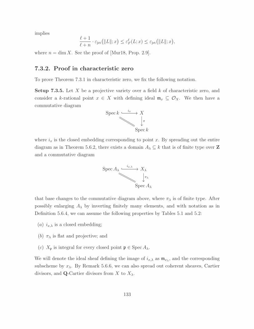
implies`+ 1

`+ n· εjet

(‖L‖;x

)≤ ε`F (L;x) ≤ εjet

(‖L‖;x

),

where n = dimX. See the proof of [Mur18, Prop. 2.9].

7.3.2. Proof in characteristic zero

To prove Theorem 7.3.1 in characteristic zero, we fix the following notation.

Setup 7.3.5. Let X be a projective variety over a field k of characteristic zero, and

consider a k-rational point x ∈ X with defining ideal mx ⊆ OX . We then have a

commutative diagram

Spec k X

Spec k

ix

π

where ix is the closed embedding corresponding to point x. By spreading out the entire

diagram as in Theorem 5.6.2, there exists a domain Aλ ⊆ k that is of finite type over Z

and a commutative diagram

SpecAλ Xλ

SpecAλ

ix,λ

πλ

that base changes to the commutative diagram above, where πλ is of finite type. After

possibly enlarging Aλ by inverting finitely many elements, and with notation as in

Definition 5.6.4, we can assume the following properties by Tables 5.1 and 5.2:

(a) ix,λ is a closed embedding;

(b) πλ is flat and projective; and

(c) Xp is integral for every closed point p ∈ SpecAλ.

We will denote the ideal sheaf defining the image of ix,λ as mxλ , and the corresponding

subscheme by xλ. By Remark 5.6.6, we can also spread out coherent sheaves, Cartier

divisors, and Q-Cartier divisors from X to Xλ.

133

We will also need the following result, which describes how separation of jets and

how εjet(‖D‖;x) behave under reduction modulo p. We note that in the description of

different loci below, we allow q to be non-closed points in SpecAλ.

Lemma 7.3.6. Let X and mx be as in Setup 7.3.5, with models Xλ and mxλ over

SpecAλ, respectively.

(i) Let F be a coherent sheaf on X together with a model Fλ over SpecAλ. Let ` ≥ −1

be an integer, and suppose that Fλ and Fλ/m`+1xλ

Fλ are flat and cohomologically

flat in degree zero over SpecAλ. Then, the locus

q ∈ SpecAλ

∣∣ Fq separates `-jets at xq

is open in SpecAλ.

(ii) Let D be a Q-Cartier divisor on X together with a model Dλ over SpecAλ. Then,

for every integer m > 0 such that mDλ is Cartier, the locus

q ∈ SpecAλ

∣∣ mDq separates `-jets at xq

contains an open set in SpecAλ for every integer ` ≥ −1.

(iii) Let D be a Q-Cartier divisor on X together with a model Dλ over SpecAλ, and let

δ > 0 be a real number such that εjet(‖D‖;x) > δ. Then, the locus

q ∈ SpecAλ

∣∣ εjet

(‖Dq‖;xq

)> δ

(7.9)

contains a non-empty open set in SpecAλ.

Proof. We first prove (i). By cohomology and base change [Ill05, Cor. 8.3.11], the locus

where Fq does not separate `-jets at xq is

Supp(

coker(πλ∗Fλ −→ πλ∗(Fλ/m

`+1xλ

Fλ))),

where πλ : Xλ → SpecAλ is as in Setup 7.3.5. Since πλ is proper, both direct image

sheaves are coherent, and the cokernel above is also coherent. Thus, the support of this

cokernel is closed in SpecAλ, which implies (i). (ii) then follows from (i) by setting

134

F = OX(mD), after possibly enlarging Aλ by inverting finitely many elements to assume

that OXλ(mDλ) and OXλ(mDλ)⊗OXλ/m`+1xλ

are flat and cohomologically flat in degree

zero over SpecAλ by generic flatness [EGAIV2, Thm. 6.9.1] and by [Ill05, Cor. 8.3.11].

We now show (iii). By Lemma 7.2.5, εjet(‖D‖;x) is a limit, hence there exists an

integer m > 0 such that mD is a Cartier divisor, and such that

s(mD;x)

m> δ. (7.10)

Since s(mD;x) is an integer, this inequality is equivalent to s(mD;x) ≥ bmδc+ 1. By

(ii), the locus

q ∈ SpecAλ

∣∣ mDq separates(bmδc+ 1

)-jets at xq

(7.11)

contains an open set, which is nonempty by (7.10) since the generic point of SpecAλ is

contained in this set by flat base change, and since Aλ ⊆ k is flat. Now if mDq separates

(bmδc+ 1)-jets at xq, then we have the inequality

ε(‖Dq‖;xq

)≥ s(mDq;x)

m> δ

by the fact that s(mDq;x) is an integer. The locus (7.11) is therefore contained in the

locus (7.9), and (iii) follows.

We will also use the following:

Lemma 7.3.7. Let X be as in Setup 7.3.5, with a model Xλ over SpecAλ. If ωiXλ/Aλ is

flat over Aλ for every i, then the base change isomorphism

ω•Xλ/Aλ |LXp

∼−→ ω•Xp

from [Lip09, Cor. 4.4.3] induces an isomorphism

ωXλ/Aλ |Xp

∼−→ ωXp .

Proof. This statement follows from the flatness of ωiXλ/Aλ and a spectral sequence for

sheaf Tor ; see [EGAIII2, Cor. 6.5.9].

135

We can now prove Theorem 7.3.1 in characteristic zero via reduction modulo p.

Proof of Theorem 7.3.1 in characteristic zero. As in the proof in positive characteristic,

we note that

εjet

(‖L‖;x

)> n+ `

by Proposition 7.2.10, where for (i), we note that ε(L;x) > n + ` implies x /∈ B+(L)

by Theorem 4.6.6 and [Laz04a, Prop. 5.1.9]. We use the notation in Setup 7.3.5. After

possibly further enlarging Aλ by inverting finitely many elements, we may assume that

(a) the Cartier divisor L spreads out to a Cartier divisor Lλ on Xλ such that OXλ(Lλ)

is flat and cohomologically flat in degree zero over Aλ;

(b) the sheaves ωiXλ/Aλ and ωXλ/Aλ are flat and cohomologically flat in degree zero over

Aλ for every i; and

(c) the sheaf ωXλ/Aλ ⊗OXλ(Lλ)⊗OXλ/m`+1xλ

is flat and cohomologically flat in degree

zero over Aλ.

Here, we have used Remark 5.6.6, generic flatness [EGAIV2, Thm. 6.9.1], and cohomology

and base change [Ill05, Cor. 8.3.11].

We can now prove Theorem 7.3.1 in characteristic zero. First, we have a base change

isomorphism

ωXλ/Aλ|Xp

∼−→ ωXp

by Lemma 7.3.7 and the assumption (b). Since OX(Lλ) is also flat and cohomologically

flat in degree zero over SpecAλ, the sheaf ωXλ/Aλ ⊗OXλ(Lλ) is a model of ωX ⊗OX(L)

over SpecAλ, and is flat and cohomologically flat in degree zero over SpecAλ.

We now claim that ωXp ⊗ OXp(Lp) separates `-jets at xp for some closed point p ∈SpecAλ. Note that εjet(‖Lp‖;xp) > n + ` holds for all p in an open dense subset of

SpecAλ by Lemma 7.3.6(iii). We now claim we can apply Theorem 7.3.2 to show that

ωXp ⊗OXp(Lp) separates `-jets at xp for all p such that εjet(‖Lp‖;xp) > n+ ` and such

that Xp is F -injective. First, we note that κ(p) is F -finite for all p ∈ SpecAλ, since it

is a finite field by Lemma 5.6.5. Thus, Lemma A.9 implies that the Frobenius trace

TrXp : F∗ωXp → ωXp on Xp exists and is surjective. We can therefore apply Theorem 7.3.2

to show that ωXp ⊗OXp(Lp) separates `-jets at xp.

136

Finally, we show that ωX⊗OX(L) separates `-jets at x. Since the extension FracAλ ⊆ k

is flat, it suffices by flat base change to show that ωXη ⊗OXη(Lη) separates `-jets at xη,

where η ∈ SpecAλ is the generic point. But this follows from the previous paragraph

from Lemma 7.3.6(i), since ωXp ⊗OXp(Lp) separates `-jets at xp for some closed point

p ∈ SpecAλ.

137

Chapter 8

The Angehrn–Siu theorem

The goal of this chapter is to prove the following version of the Angehrn–Siu theorem

[AS95, Thm. 0.1].

Theorem D. Let (X,∆) be an effective log pair, where X is a normal projective variety

over an algebraically closed field k of characteristic zero, ∆ is a Q-Weil divisor, and

KX + ∆ is Q-Cartier. Let x ∈ X be a closed point such that (X,∆) is klt at x, and let

D be a Cartier divisor on X such that setting H := D − (KX + ∆), there exist positive

numbers c(m) with the following properties:

(i) For every positive dimensional variety Z ⊆ X containing x, we have

volX|Z(H) > c(dimZ)dimZ .

(ii) The numbers c(m) satisfy the inequality

dimX∑

m=1

m

c(m)≤ 1.

Then, OX(D) has a global section not vanishing at x.

Before we prove this statement, we will need to prove a replacement for the Nadel

vanishing theorem [Laz04b, Thm. 9.4.17].

138

8.1. The lifting theorem

A major obstacle in proving the Angehrn–Siu theorem in positive characteristic is that

Kodaira-type vanishing theorems are false; see Example 2.4.4. While the result below

is not yet strong enough to prove their theorem in positive characteristic, it does give

a replacement for the Nadel vanishing theorem in characteristic zero, after reduction

modulo p.

We start by stating the characteristic zero version of the result.

Theorem C. Let (X,∆) be an effective log pair such that X is a projective normal

variety over a field k of characteristic zero, and such that KX +∆ is Q-Cartier. Consider

a k-rational point x ∈ X such that (X,∆) is of dense F -pure type at x. Suppose that D

is a Cartier divisor on X such that H = D − (KX + ∆) satisfies

ε(‖H‖;x

)> lctx

((X,∆);mx

).

Then, OX(D) has a global section not vanishing at x.

Note that in Chapter 1, we stated Theorem C with “dense F -pure type” replaced

by “klt.” The formulation in Chapter 1 follows from this one since klt pairs are

of dense strongly F -regular type by Theorem 5.6.8, hence of dense F -pure type by

Proposition 5.4.3(iv).

Theorem C follows from the following result via reduction modulo p.

Theorem 8.1.1. Let (X,∆) be an effective log pair such that X is a projective normal

variety over an F -finite field k of characteristic p > 0, and such that KX+∆ is Q-Cartier.

Consider a k-rational point x ∈ X such that (X,∆) is F -pure at x. Suppose that D is a

Cartier divisor on X such that H = D − (KX + ∆) satisfies

εjet

(‖H‖;x

)> fptx

((X,∆);mx

).

Then, OX(D) has a global section not vanishing at x.

We first prove Theorem C, assuming Theorem 8.1.1.

Proof of Theorem C. Let Xλ, ∆λ, mxλ, and Dλ be models of X, ∆, mx, and D over a

finitely generated Z-algebra Aλ ⊆ k as in Theorem 5.6.2 and Remark 5.6.6; cf. Setup 7.3.5.

139

After possibly enlarging Aλ by inverting finitely many elements, we may assume that Xp

is normal for every p ∈ Aλ (by Table 5.2), and moreover, we may assume that ωXλ/Aλ is

a model for ωX ' OX(KX) (by Lemma 7.3.7) that is flat and cohomologically flat over

SpecAλ (by generic flatness [EGAIV2, Thm. 6.9.1] and cohomology and base change

[Ill05, Cor. 8.3.11]). By assumption, (Xp,∆p) is F -pure for a dense set of p ∈ SpecAλ,

and we can also assume that for these p, the F -pure threshold of (Xp,∆p) with respect

to mxp is strictly less than εjet(‖H‖;x) by Theorem 5.6.8. Note that here we have used

Proposition 7.2.10 to say that ε(‖H‖;x) = εjet(‖H‖;x). By Lemma 7.3.6(iii), we have

εjet

(‖Hp‖;xp

)> fptx

((Xp,∆p);mxp

)

for all but finitely many p ∈ SpecAλ, where Hp = Dp − (KXp + ∆p). Theorem 8.1.1

therefore implies that OX(Dp) has a global section not vanishing at xp after reduction

modulo p for infinitely many p ∈ SpecA, where we note that κ(p) is F -finite for every

p ∈ SpecAλ, since κ(p) is a finite field by Lemma 5.6.5. Thus, OXη(Dη) has a global

section not vanishing at xη by Lemma 7.3.6(i), where η ∈ SpecAλ is the generic point.

Finally, since FracAλ ⊆ k is flat, we see that OX(D) also has a global section not

vanishing at x by flat base change.

We now prove Theorem 8.1.1.

Proof of Theorem 8.1.1. We proceed in a sequence of steps, following the outline of the

proof of [MS14, Thm. 3.1] and [Mur18, Thm. C].

Denoting by c the F -pure threshold fptx((X,∆);mx) of (X,∆) with respect to mx, fix

δ > 0 such that

εjet(‖H‖;x) > (1 + 2δ)c.

We first claim that there exists a positive integer m0 and a sequence de such that

m0H is Cartier, OX(m0deH) separates (b(pe − 1)(1 + δ)cc − 1)-jets at x for all e > 0,

and pe −m0de →∞ as e→∞. By Lemma 7.2.5, there exists a positive integer m0 such

that m0H is Cartier and

s(m0H;x)

m0

> (1 + 2δ)c.

140

Now for every integer e > 0, let

de =

⌈b(pe − 1)(1 + δ)cc − 1

s(m0H;x)

⌉.

By the superadditivity property (Lemma 7.2.5), we have

s(m0deH;x) ≥ de · s(m0H;x) ≥ b(pe − 1)(1 + δ)cc − 1,

hence OX(m0deH) separates (b(pe − 1)(1 + δ)cc − 1)-jets at x. We now claim that

pe −m0de →∞ as e→∞. Note that

pe −m0de = pe −m0 ·⌈b(pe − 1)(1 + δ)cc − 1

s(m0H;x)

⌉

≥ pe −(b(pe − 1)(1 + δ)cc − 1

)· m0

s(m0H;x)−m0

≥ pe − b(pe − 1)(1 + δ)cc − 1

(1 + 2δ)c−m0

and as e→∞, we have

lime→∞

(pe −m0de) ≥ lime→∞

(pe − b(p

e − 1)(1 + δ)cc − 1

(1 + 2δ)c−m0

)

= lime→∞

pe(

1− 1 + δ

1 + 2δ

)−m0 =∞.

We therefore see that OX(m0deH) separates (b(pe − 1)(1 + δ)cc − 1)-jets at x, and that

pe −m0de →∞ as e→∞.

We now show that there exists a positive integer e such that OX(dKX + ∆ + peHe)separates (b(pe−1)(1 + δ)cc−1)-jets at x. Let m0 and de as in the previous paragraph.

Since x /∈ B+(H) and since pe −m0de →∞, Proposition 4.6.7 implies that the sheaf

OX(dKX + ∆ + (pe −m0de)He

)

is globally generated at x for all e 0. SinceOX(m0deH) separates (b(pe−1)(1+δ)cc−1)-

141

jets at x, Lemma 7.2.5 implies

OX(dKX + ∆ + (pe −m0de)He

)⊗OX(m0deH) ' OX

(dKX + ∆ + peHe

)

separates (b(pe − 1)(1 + δ)cc − 1)-jets at x.

We now use the trace morphism TreX,b(pe−1)∆c to take out the factors of pe. Note

that TreX,b(pe−1)∆c is surjective at x by assumption, since (X,∆) is F -pure at x (Corol-

lary 5.4.7(i)). Twisting TreX,b(pe−1)∆c by OX(D), we have a morphism

F e∗(OX((1− pe)KX − b(pe − 1)∆c+ peD

)) TreX,b(pe−1)∆c(D)

−−−−−−−−−−→ OX(D) (8.1)

that is surjective at x, where the source can be identified with

F e∗(OX(d(1− pe)(KX + ∆) + peDe

))= F e

∗(OX(dKX + ∆ + peHe

)).

The triple (X,∆,m(1+δ)cx ) is not F -pure, since c is the F -pure threshold fptx((X,∆);mx).

Thus, the morphism

F e∗(mb(p

e−1)(1+δ)ccx · OX

(dKX + ∆ + peHe

)) TreX,b(pe−1)∆c(D)

−−−−−−−−−−→ OX(D) (8.2)

induced by the trace morphism (8.1) is not surjective at x by Corollary 5.4.7. We

therefore see that the morphism (8.2) induces a morphism

F e∗(mb(p

e−1)(1+δ)ccx · OX

(dKX + ∆ + peHe

)) TreX,b(pe−1)∆c(D)

−−−−−−−−−−→ mx · OX(D)

since the target is OX,y(D) after localizing at every point y 6= x, and at x, the non-

surjectivity of the localization of (8.2) at x is equivalent to having image in mx · OX,x(D),

142

by the fact that OX,x is local. We therefore have the commutative diagram

0 0

F e∗(mb(pe−1)(1+δ)ccx · OX

(dKX + ∆ + peHe

))mx · OX(D)

F e∗(OX(dKX + ∆ + peHe

))OX(D)

F e∗

(OX(dKX + ∆ + peHe

)

mb(pe−1)(1+δ)ccx · OX

(dKX + ∆ + peHe

))

OX(D)

mx · OX(D)

0 0

where the bottom two horizontal arrows are induced by TreX,b(pe−1)∆c, and are therefore

surjective at x. Note that the left column is exact since the Frobenius morphism F is

affine. Taking global sections in the bottom square, we obtain the following commutative

square:

H0(X,OX

(dKX + ∆ + peHe

))H0(X,OX(D)

)

H0

(X,

OX(dKX + ∆ + peHe

)

mb(pe−1)(1+δ)ccx · OX

(dKX + ∆ + peHe

))

H0

(X,

OX(D)

mx · OX(D)

)ϕ

ψ

where ψ is surjective since the corresponding morphism of sheaves is a surjective morphism

of skyscraper sheaves supported at x. Since the restriction map ϕ is surjective by the

previous paragraph, the right vertical map is necessarily surjective by the commutativity

of the diagram. Thus, the sheaf OX(D) has a global section not vanishing at x.

Remark 8.1.2. One can also prove a weaker version of Theorem 8.1.1 using another

variant of Frobenius–Seshadri constants (cf. Remark 7.3.4). The relevant version of the

Seshadri constant is defined using the Frobenius degeneracy ideals first introduced by

Yao [Yao06, Rem. 2.3(1)] and Aberbach–Enescu [AE05, Def. 3.1]. If (R,∆) is a sharply

143

F -pure pair where R is an F -finite local ring of characteristic p > 0 with maximal ideal

m ⊆ R, then following [Tuc12, Def. 4.3; BST12, Def. 3.3], the eth Frobenius degeneracy

ideal is

I∆e (m) :=

f ∈ R

∣∣∣ ϕ(f) ∈ m for all ϕ ∈ HomR

(F e∗R(d(pe − 1)∆e), R

).

Note that we have followed the terminology from [CRST, Def. 2.6]. Following [DSNB18,

Lem. 3.9 and Prop. 3.10], one can show that

mbpe fpt((R,∆);m)c+1 ⊆ I∆

e (m). (8.3)

Now let (X,∆) be a sharply F -pure pair, where X is a complete variety over an F -finite

field of characteristic p > 0. For a Q-Cartier divisor H on X and for every integer m ≥ 1

such that mH is a Cartier divisor, denote by s∆F -sig(mH;x) the largest integer such that

the restriction map

H0(X,OX(mH)

)−→ H0

(X,OX(mH)⊗OX/I∆

e (mx))

is surjective. Then, the F -signature Seshadri constant of H at x is

ε∆F -sig(H;x) := lim sup

m→∞

ps∆F -sig(mH;x) − 1

m,

where the limit supremum runs over all m such that mH is integral. The inclusion (8.3)

then implies

εjet

(‖H‖;x

)≤ fptx

((X,∆);mx

)· ε∆

F -sig(H;x).

Using the strategy in Theorem 8.1.1, one can show that a lower bound of the form

ε∆F -sig(H;x) > 1 implies the existence of global sections of OX(D) as in Theorem 8.1.1.

This version of the Frobenius–Seshadri constant is difficult to work with since we do not

know if the analogues of [MS14, Lem. 2.5 and Prop. 2.6] or [Mur18, Lem. 2.4 and Prop.

2.5] hold. The core issue is that the sequence I∆e (mx)e∈N does not necessarily form a

p-family of ideals in the sense of [HJ18, Def. 1.1].

144

8.2. Constructing singular divisors and proof of

Theorem D

The goal in this section is to prove the following result, which will be the other crucial

ingredient in proving Theorem D.

Theorem 8.2.1 (cf. [Kol97, Thm. 6.4]). Let (X,∆) be an effective log pair, where X is

a normal projective variety over an algebraically closed field k of characteristic zero, ∆

is a Q-Weil divisor, and KX + ∆ is Q-Cartier. Let x ∈ X be a closed point such that

(X,∆) is klt at x. Let D be a Cartier divisor on X such that setting N := D− (KX + ∆),

there exist positive numbers c(m) with the following properties:

(i) For every positive dimensional variety Z ⊆ X containing x, we have

volX|Z(N) > c(dimZ)dimZ .

(ii) The numbers c(m) satisfy the inequality

dimX∑

m=1

m

c(m)≤ 1.

Then, there exist an effective Q-Cartier Q-Weil divisor E ∼Q bN for some b ∈ (0, 1), and

an open neighborhood X0 ⊆ X of x such that (X0,∆ + E) is log canonical, (X0,∆ + E)

is klt on X0 r x, and (X,∆ + E) is not klt at x.

Assuming this, Theorem D is not difficult.

Proof of Theorem D. Fix a closed point x ∈ X. By Theorem 8.2.1, there exists a

boundary divisor E ∼Q bN for some b ∈ (0, 1) such that (X,∆ + E) is strictly log

canonical at x, but is klt in a punctured neighborhood of x. Now let f : Y → X be

a log resolution for (X,∆ + E,mx). Then, there is divisor F ⊆ Y over x such that

a(F,X,∆ + E) = −1 by Lemma 4.8.5. For 0 < δ 1, we claim that (X,∆ + (1− δ)E)

is klt in a neighborhood of x, and that

lctx((X,∆ + (1− δ)E);mx

)< (1− b) · ε

(‖N‖;x

).

145

Note that the right-hand side is positive since b ∈ (0, 1). The property that (X,∆ +

(1 − δ)E) is klt in a neighborhood of x follows from Lemma 4.8.5, and the inequality

above follows for 0 < δ 1 from the computation of the log canonical threshold in

Proposition 4.8.7, since the Cartier divisor defined by f−1mx · OY contains F as a

component. We therefore have

D −(KX + ∆ + (1− δ)E

)∼Q N − (1− δ)bN =

(1− (1− δ)b

)N,

hence the conditions of Theorem C are satisfied for H = D− (KX + ∆ + (1− δ)E), since

ε(‖H‖;x

)=(1− (1− δ)b

)· ε(‖N‖;x

)>(1− b

)· ε(‖N‖;x

)

> lctx((X,∆ + (1− δ)E);mx

).

It therefore remains to show Theorem 8.2.1. The idea of the proof is to first produce

a divisor that is highly singular at a point, and then cut down the dimension of the

non-klt locus at the point until the non-klt locus is isolated. We mostly follow the proofs

in [Kol97, §6] and [Liu, §3], with suitable changes to deal with the weaker positivity

condition on N .

We start with the following result. Recall that if D is a Q-Cartier divisor on a variety

X over a field k, then a graded linear system V• associated to D is a sequence of subspaces

Vm ⊆ H0(X,OX(mD)) for m such that mD is a Cartier divisor, which satisfies the

property that the multiplication map Vm ⊗ Vn → H0(X,OX((m+ n)D)) has image in

Vm+n [Laz04a, Def. 2.4.1]. The volume of V• is

volX(V•) := lim supm→∞

dimk Vmmn/n!

,

where n = dimX [Laz04a, Def. 2.4.12]. If f : Y → X is a morphism, and V• is a graded

linear system associated to a Q-Cartier D on X, then the graded linear series f ∗V• is

given by setting

f ∗Vm := im(Vm ⊆ H0

(X,OX(mD)

)−→ H0

(Y,OY (mf ∗D)

)),

where the morphism is induced by the pullback morphism OX(mD)→ f∗OY (mf ∗D).

In particular, if f is an inclusion Y ⊆ X of a closed subvariety, then we set V•|Y := f ∗V•.

146

Lemma 8.2.2 (cf. [Kol97, Lem. 6.1; Fuj11, Lem. 12.2]). Let f : Y → Z be a surjective

projective morphism from a normal variety Y to an affine variety Z over an algebraically

closed field k, and let W be a general closed subvariety of Y such that f |W : W → Z is

generically finite and generically regular. Consider a Q-Cartier divisor M on Y , and

let V• be a graded linear system associated to M . Then, for every ε > 0, there exists a

positive integer t > 0 such that tM is a Cartier divisor, and such that there exists an

effective Cartier divisor Dt = Dt(ε) ∈ |Vt| on Y such that setting D := 1tDt, we have

multW D ≥(

volF (V•|F )

deg(f |W )

)1/n

− ε, (8.4)

where F is a general fiber of f and n = dimF .

Here, multW D is the maximum integer s such that D vanishes to order s everywhere

along W , and deg(f |W ) is the degree of the generically finite morphism f |W .

Proof. Let t > 0 be an integer such that tM is Cartier, and let IW ⊆ OY be the ideal

sheaf defining W . Then, for every integer s > 0, we have the short exact sequence

0 −→ IsW ⊗OY (tM) −→ OY (tM) −→ OY (tM)⊗OY /IW −→ 0,

and pushing forward by f , we obtain the left-exact sequence

0 −→ f∗(IsW ⊗OY (tM)

)−→ f∗

(OY (tM)

)−→ f∗

(OY (tM)⊗OY /IsW

). (8.5)

Now choose integers s, t > 0 such that

(volF (V•|F )

deg(f |W )

)1/n

>s

t>

(volF (V•|F )

deg(f |W )

)1/n

− ε,

and recall that for every regular point x ∈ F , we have

h0(F,OF/msx) =

(n+ s− 1

n

)=sn

n!+O(sn−1).

Thus, after possibly replacing s and t by multiples, we may assume without loss of

147

generality that tM is Cartier, and that

dimk Vt|F − h0(F,OF (tM |F )⊗OF/IsW∩F

)

= dimk Vt|F − deg(f |W ) ·(n+ s− 1

n

)> 0

(8.6)

by the definition of volume, which implies that Vt|F has sections vanishing to order s

everywhere along W∩F . Now by generic flatness [EGAIV2, Thm. 6.9.1] and by [Ill05, Cor.

8.3.11], the sheaf OY (tM)⊗OY /IsW is generically flat and generically cohomologically

flat in degree zero over Z. By cohomology and base change [Ill05, Cor. 8.3.11], the

estimate (8.6) together with the exact sequence (8.5) therefore implies that the sheaf

f∗(OY (tM)⊗OY /IsW ) is nonzero, hence has a global section by the fact that Z is affine.

We then let Dt = Dt(ε) be a Cartier divisor corresponding to a section in

H0(Z, f∗

(OY (tM)⊗OY /IsW

))= H0

(Y,OY (tM)⊗OY /IsW

),

in which case (8.4) holds for D := 1tDt.

When Z = Spec k is a point and W is a closed point x ∈ X, we see that Lemma 8.2.2

gives a way to construct an effective Q-Cartier divisor D(ε) that is singular at x.

However, this divisor may have very bad singularities in a neighborhood of x. The proof

of Theorem 8.2.1 is devoted to ensuring that one can replace D(ε) with a divisor with

mild singularities in a neighborhood of x.

In the course of the proof, we will need the following:

Lemma 8.2.3 (cf. [Kol97, Cor. 7.8]). Let (Y,∆) be a klt pair over an algebraically closed

field k of characteristic zero, and let y ∈ Y be a closed point. Let C be a smooth affine

curve,and let B be a Q-Cartier divisor on Y ×C such that y×C ⊆ SuppB. Let 0 ∈ Cbe a closed point such that (Y × c,∆× c+B|Y×c) is not log canonical at y for all

closed points c ∈ C in a punctured neighborhood of 0. Then, (Y ×0,∆×0+B|Y×0)is not log canonical at y.

Kollar’s proof of [Kol97, Cor. 7.8] uses the Kollar–Shokurov connectedness theorem

[Kol97, Thm. 7.4], among other results. The proof of this connectedness theorem uses

vanishing theorems. We therefore give a proof of Lemma 8.2.3 that uses reduction

modulo p instead of vanishing theorems.

148

Proof. Set X = Y × C, and suppose that (Y × 0,∆× 0+B|Y×0) is log canonical.

Then, by inversion of adjunction for log canonical pairs [Tak04b, Thm. 4.2], we see that

(X,∆× C +B + Y × 0) is log canonical in a neighborhood U ⊆ X of (y, 0). Letting

W = U ∩ (y × C), we see that

(Y × c,∆× c+ (B + Y × 0)|Y×c

)=(Y × c,∆× c+B|Y×c

)

is log canonical at y for general closed points c ∈ W by Reid’s Bertini-type theorem

[Kol97, Prop. 7.7], which is a contradiction.

We can now prove Theorem 8.2.1.

Proof of Theorem 8.2.1. We prove Theorem 8.2.1 in a sequence of steps.

Step 1. Finding a singular divisor at x.

Theorem 8.2.4 (cf. [Kol97, Thm. 6.7.1; Liu, Prop. 3.3]). Let (X,∆) be an effective

log pair, where X is a normal projective variety over an algebraically closed field k of

characteristic zero, ∆ is a Q-Weil divisor, and KX + ∆ is Q-Cartier. Consider a closed

point x ∈ X such that (X,∆) is klt at x. Let H be a Q-Cartier divisor on X, and let V•

be a graded linear system associated to H such that volX(V•) > nn. Then, there exists

an effective Q-divisor Bx ∼Q H that is a multiple of a divisor in |Vt| for some t such

that (X,∆ +Bx) is not log canonical at x.

Proof. If x ∈ X is a regular point, then this immediately follows from Lemma 8.2.2 by

setting Z = Spec k and W = x. Otherwise, consider the second projection morphism

X ×A1k → A1

k, and let C ′ ⊆ X ×A1k be a general curve passing through (x, 0) that is

finite over A1k. Let ν : C → C ′ be the normalization of C ′. We then have the commutative

diagram

C

X × C X ×A1k

C C ′ A1k

σ

p2 p2

ν

where the outer rectangle is cartesian. By the universal property of fiber products, this

cartesian rectangle induces a section σ : C → X × C of p2 : X × C → C, such that σ(C)

149

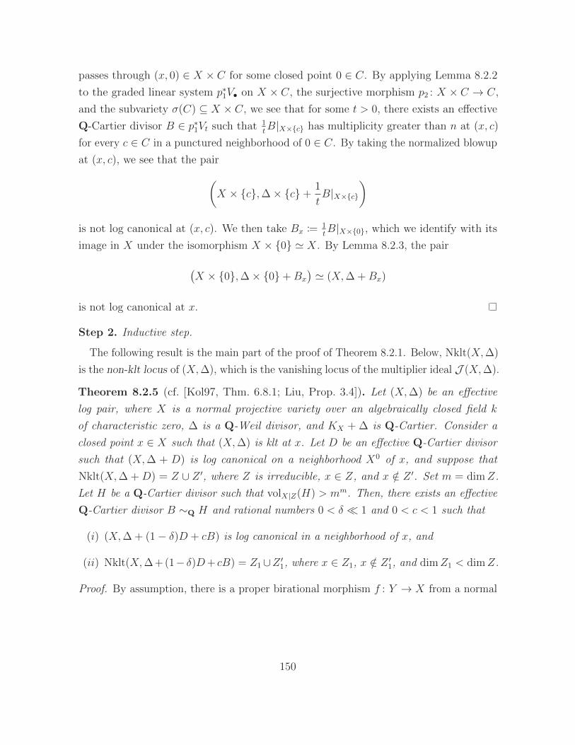
passes through (x, 0) ∈ X × C for some closed point 0 ∈ C. By applying Lemma 8.2.2

to the graded linear system p∗1V• on X × C, the surjective morphism p2 : X × C → C,

and the subvariety σ(C) ⊆ X × C, we see that for some t > 0, there exists an effective

Q-Cartier divisor B ∈ p∗1Vt such that 1tB|X×c has multiplicity greater than n at (x, c)

for every c ∈ C in a punctured neighborhood of 0 ∈ C. By taking the normalized blowup

at (x, c), we see that the pair

(X × c,∆× c+

1

tB|X×c

)

is not log canonical at (x, c). We then take Bx := 1tB|X×0, which we identify with its

image in X under the isomorphism X × 0 ' X. By Lemma 8.2.3, the pair

(X × 0,∆× 0+Bx

)' (X,∆ +Bx)

is not log canonical at x.

Step 2. Inductive step.

The following result is the main part of the proof of Theorem 8.2.1. Below, Nklt(X,∆)

is the non-klt locus of (X,∆), which is the vanishing locus of the multiplier ideal J (X,∆).

Theorem 8.2.5 (cf. [Kol97, Thm. 6.8.1; Liu, Prop. 3.4]). Let (X,∆) be an effective

log pair, where X is a normal projective variety over an algebraically closed field k

of characteristic zero, ∆ is a Q-Weil divisor, and KX + ∆ is Q-Cartier. Consider a

closed point x ∈ X such that (X,∆) is klt at x. Let D be an effective Q-Cartier divisor

such that (X,∆ + D) is log canonical on a neighborhood X0 of x, and suppose that

Nklt(X,∆ +D) = Z ∪ Z ′, where Z is irreducible, x ∈ Z, and x /∈ Z ′. Set m = dimZ.

Let H be a Q-Cartier divisor such that volX|Z(H) > mm. Then, there exists an effective

Q-Cartier divisor B ∼Q H and rational numbers 0 < δ 1 and 0 < c < 1 such that

(i) (X,∆ + (1− δ)D + cB) is log canonical in a neighborhood of x, and

(ii) Nklt(X,∆ + (1− δ)D+ cB) = Z1∪Z ′1, where x ∈ Z1, x /∈ Z ′1, and dimZ1 < dimZ.

Proof. By assumption, there is a proper birational morphism f : Y → X from a normal

150

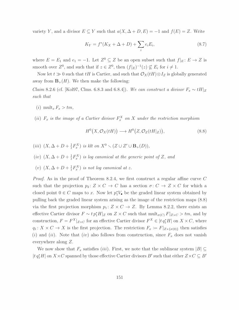
variety Y , and a divisor E ⊆ Y such that a(X,∆ +D,E) = −1 and f(E) = Z. Write

KY = f ∗(KX + ∆ +D) +∑

i

eiEi, (8.7)

where E = E1 and e1 = −1. Let Z0 ⊆ Z be an open subset such that f |E : E → Z is

smooth over Z0, and such that if z ∈ Z0, then (f |E)−1(z) 6⊆ Ei for i 6= 1.

Now let t 0 such that tH is Cartier, and such that OX(tH)⊗IZ is globally generated

away from B+(H). We then make the following:

Claim 8.2.6 (cf. [Kol97, Clms. 6.8.3 and 6.8.4]). We can construct a divisor Fx ∼ tH|Zsuch that

(i) multx Fx > tm,

(ii) Fx is the image of a Cartier divisor FXx on X under the restriction morphism

H0(X,OX(tH)

)−→ H0

(Z,OZ(tH|Z)

), (8.8)

(iii) (X,∆ +D + 1tFXx ) is klt on X0 r (Z ∪ Z ′ ∪B+(D)),

(iv) (X,∆ +D + 1tFXx ) is log canonical at the generic point of Z, and

(v) (X,∆ +D + 1tFXx ) is not log canonical at z.

Proof. As in the proof of Theorem 8.2.4, we first construct a regular affine curve C

such that the projection p2 : Z × C → C has a section σ : C → Z × C for which a

closed point 0 ∈ C maps to x. Now let p∗1V• be the graded linear system obtained by

pulling back the graded linear system arising as the image of the restriction maps (8.8)

via the first projection morphism p1 : Z × C → Z. By Lemma 8.2.2, there exists an

effective Cartier divisor F ∼ t p∗1H|Z on Z × C such that multσ(C) F |Z×C > tm, and by

construction, F = FX |Z×C for an effective Cartier divisor FX ∈ |t q∗1H| on X ×C, where

q1 : X × C → X is the first projection. The restriction Fx := F |Z×σ(0) then satisfies

(i) and (ii). Note that (iv) also follows from construction, since Fx does not vanish

everywhere along Z.

We now show that Fx satisfies (iii). First, we note that the sublinear system |B| ⊆|t q∗1H| on X×C spanned by those effective Cartier divisors B′ such that either Z×C ⊆ B′

151

or B′|Z×C = F is basepoint-free on (X r (Z ∪ B+(H))) × C by the assumption that

OX(tH) ⊗ IZ is globally generated away from B+(H). Thus, (iii) follows from the

Kollar–Bertini theorem [Kol97, Thm. 4.8.2] by choosing FX generally in |B|.It remains to show (v). By Lemma 8.2.3, it suffices to show that for every 0 6= c ∈ C

such that σ(c) ∈ Z0, the pair (X,∆ + D + 1tFXσ(c)) is not log canonical at σ(c), where

FXσ(c) := F |X×σ(c). Let y be the generic point of (f |E)−1(σ(c)). Writing (8.7) as before,

we also write

f ∗FXσ(c) = F Y

σ(c) +∑

i

tfiEi

where F Yσ(c) is the strict transform f−1

∗ FXσ(c) of FX

σ(c). We then have

KY +1

tF Yσ(c) +

∑(fi − ei)Ei ∼Q f ∗

(KX + ∆ +D +

1

tFXσ(c)

).

Now (X,∆ +D + 1tFXσ(c)) is not log canonical at σ(c) if (Y, 1

tF Yσ(c) +

∑(fi − ei)Ei) is not

sub-log canonical at y. Since Z 6⊆ FXσ(c), we know that f1 = 0. Thus,

∑(fi − ei)Ei =

E +∑

i 6=1(fi− ei)Ei, and by assumption none of the Ei contain y when i 6= 1. Moreover,

(Y, 1tF Yσ(c) +

∑(fi − ei)Ei) is not sub-log canonical at y if and only if (Y, 1

tF Yσ(c) + E) is

not log canonical at y. By inversion of adjunction [Tak04b, Thm. 4.2], the latter holds

if and only if (E, 1tf ∗FX

σ(c)|E) = (E, 1t(f |E)∗Fσ(c)) is not log canonical at y. Now E is

smooth at y, and y has codimension m in E and 1t(f |E)∗Fσ(c) has multiplicity > m. We

then see that (E, 1t(f |E)∗Fσ(c)) is not log canonical at y by taking the normalized blowup

at y. This concludes the proof of Claim 8.2.6.

To finish the proof of Theorem 8.2.5, we apply Claim 8.2.6 and set B = 1tFXx . Note

that (X,∆ + (1− δ)D) is klt at the generic point of Z for every δ > 0 by the assumptions

that (X,∆) is klt, that (X,∆ +D) is log canonical in a neighborhood of x, and on the

non-klt locus of (X,∆ +D). Now choose 0 < δ 1 such that (X,∆ + (1− δ)D +B) is

not log canonical at x. Letting c be the log canonical threshold of (X,∆ + (1 − δ)D)

with respect to B, we then see that (X,∆ + (1 − δ)D + cB) is log canonical but not

klt at x, and that Nklt(X,∆ + (1− δ)D + cB) = Z1 ∪ Z ′1, where x ∈ Z1, x /∈ Z ′1, and

dimZ1 < dimZ.

We can almost show Theorem 8.2.1 using Theorem 8.2.5 and induction. However, the

resulting pair in Theorem 8.2.5 may be such that Nklt(X,∆ + (1− δ)D + cB) has many

152

irreducible components passing through x. We take care of this using the following:

Step 3. Tie breaking.

Lemma 8.2.7 (cf. [Kol97, Lem. 6.9.1]). Let (X,∆) be an effective log pair, where X is

a normal projective variety over a field k of characteristic zero, ∆ is a Q-Weil divisor,

and KX + ∆ is Q-Cartier. Consider a k-rational point x ∈ X such that (X,∆) is klt at

x. Let D be an effective Q-Cartier divisor on X such that (X,∆ +D) is log canonical

in a neighborhood of x. Let Nklt(X,∆ +D) =⋃i Zi be the irreducible decomposition of

Nklt(X,∆ +D), where we label Z1 such that x ∈ Z1. Let H be a Q-Cartier divisor on

X such that x /∈ B+(H). Then, for every 0 < δ 1, there is an effective Q-Cartier

divisor B ∼Q H and 0 < c < 1 such that

(i) (X,∆ + (1− δ)D + cB) is log canonical in a neighborhood of x, and

(ii) Nklt(X,∆ + (1− δ)D + cB) = W ∪W ′ where x ∈ W , x /∈ W ′, and W ⊆ Z1.

Proof. Let t 1 such that tH is Cartier and such that OX(tH) ⊗ IZ1 is globally

generated away from B+(H) (Proposition 4.6.7). Let B′ correspond to a general section

in H0(X,OX(tH) ⊗ IZ1). By the Kollar–Bertini theorem [Kol97, Thm. 4.8.2], we see

that (X,∆ + (1− δ)D+ bB′) is klt outside Z1 in a neighborhood of x for b < 1. However,

it is not log canonical along Z1 for 1 > b δ > 0. Now choose b = 1/t and 1/t δ > 0.

Then, by letting c ∈ (0, 1) be the log canonical threshold of (X,∆ + (1 − δ)D) with

respect to (1/t)B′, we see that (X,∆ + (1− δ)D + (c/t)B′) is log canonical but not klt

at x. We can then set B = 1tB′.

Step 4. Proof of Theorem 8.2.1.

We prove the following theorem by induction on j.

Theorem 8.2.8. With notation as in Theorem 8.2.1, let j ∈ 1, 2, . . . , n. Then, for

every

dj ≥n∑

m=n−j

m

c(m), (8.9)

there exists an effective Q-Cartier divisor Dj ∼Q djN and an open neighborhood X0 ⊆ X

of x such that for some bj ∈ (0, 1), we have that

(i) (X0,∆ + bjDj) is log canonical,

153

(ii) codim(Nklt(X0,∆ + bjDj), X0) ≥ j, and

(iii) (X,∆ + bjDj) is not klt at x.

Proof. Set D0 = ∅. By induction, we will assume that Dj has already been constructed,

and we are trying to construct Dj+1.

For j + 1 = 1, we construct D1 by applying Theorem 8.2.4, and set b1 to be the

log canonical threshold lctx((X,∆);D1). Now consider the case when j + 1 > 1. First

choose a positive real number ε < (j + 1) · c(j + 1)−1. By Lemma 8.2.7 and by inductive

hypothesis, there exists a Q-Cartier divisor Bj ∼Q εN such that for some δ > 0, the

Q-Cartier divisor

D′j := (1− δ)bjDj +Bj ∼Q

((1− δ)bjdj + ε

)N

satisfies conditions (i)–(iii) for bj replaced by 1, and in addition, either Z := Nklt(X0,∆+

D′j) is irreducible of codimension at least j at x, or it has codimension at least j + 1 at

x. In the latter case, let M be a general member of |tN | for t 1. By assumption in

(8.9), for all rational numbers 0 < γ 1, we have dj+1 ≥ (1 + γ)((1− δ)bjdj + ε). Thus,

we can set

Dj+1 := (1 + γ)D′j +1

t

(dj+1 − (1 + γ)

((1− δ)bjdj + ε

))M ∼Q dj+1N,

and this Q-divisor Dj+1 satisfies conditions (i)–(iii) for bj+1 = 1/(1 + γ).

It remains to consider the case when Z is irreducible of codimension at least j at x.

Set H = ((j + 1) · c(j + 1)−1 − ε)N . For 0 < ε 1, we have that (Hj · Z) > jj, hence

we can apply Theorem 8.2.5 to obtain a Q-Cartier divisor

Dj+1 ∼Q

((j + 1) · c(j + 1)−1 − ε

)N

satisfying conditions (i)–(iii) for bj+1 replaced by the rational number c in the statement

of Theorem 8.2.5.

Finally, the case j = dimX in Theorem 8.2.8 is Theorem 8.2.1, concluding the proof

of Theorem 8.2.1.

154

Appendix A

F -singularities for non-F -finite rings

In this appendix, we review classes of singularities defined using the Frobenius morphism,

taking care to avoid F -finiteness assumptions. Most of this material is well-known, but

some of the implications in Figure A.1 are new, at least for non-F -finite rings. We

recommend [TW18] for a survey of F -singularities (mostly in the F -finite setting), and

[DS16, §6] and [Has10a, §3] as references for the material on strong F -regularity in the

non-F -finite setting. Some of this material appears in [Mur, Apps. A and B] and [DM].

To define different versions of F -rationality, we will need the following:

Definition A.1 [HH90, Def. 2.1]. Let R be a noetherian ring. A sequence of elements

x1, x2, . . . , xn ∈ R is a sequence of parameters if, for every prime ideal p containing

(x1, x2, . . . , xn), the images of x1, x2, . . . , xn in Rp are part of a system of parameters

in Rp. An ideal I ⊆ R is a parameter ideal if I can be generated by a sequence of

parameters in R.

We now begin defining different classes of singularities. We start with F -singularities

defined using tight closure. Recall that if R is a ring, then R is the complement of the

union of the minimal primes of R.

Definition A.2 [HH90, Def. 8.2]. Let R be a ring of characteristic p > 0, and let

ι : N →M be an inclusion of R-modules. The tight closure of N in M is the R-module

N∗M :=

x ∈M

∣∣∣∣∣there exists c ∈ R such that for all e 0,

x⊗ c ∈ im(id⊗ ι : N ⊗R F e

∗R→M ⊗R F e∗R).

155

We say that N is tightly closed in M if N∗M = N .

Definition A.3 (F -singularities via tight closure). Let R be a noetherian ring of

characteristic p > 0. We say that

(a) R is strongly F -regular if N∗M = N for every inclusion N → M of R-modules

[Hoc07, Def. on p. 166];

(b) R is weakly F -regular if I∗R = I for every ideal I ⊆ R [HH90, Def. 4.5];

(c) R is F -regular if Rp is weakly F -regular for every prime ideal p ⊆ R [HH90, Def.

4.5];

(d) R is F -rational if I∗R = I for every parameter ideal I ⊆ R [FW89, Def. 1.10].

The original definition of F -regularity asserted that localizations at every multiplicative

set are weakly F -regular, but (c) is equivalent to this definition by [HH90, Cor. 4.15].

Remark A.4. Note that (a) is not the usual definition of strong F -regularity, although it

coincides with the usual definition (Definition A.7(a)) for F -finite rings; see Figure A.1.

Next, we define F -singularities via purity of homomorphisms involving the Frobenius.

We recall that a ring homomorphism ϕ : R→ S is pure if the induced homomorphism

idM ⊗R ϕ : M ⊗R R→M ⊗R S is injective for every R-module M . To simplify notation,

we fix the following:

Notation A.5. Let R be a ring of characteristic p > 0. For every c ∈ R and every

integer e > 0, we denote by λec the composition

RF e−→ F e

∗RF e∗ (−·c)−−−−→ F e

∗R.

Definition A.6 (F -singularities via purity). Let R be a noetherian ring of characteristic

p > 0. For every c ∈ R, we say that R is F -pure along c if λec is pure for some e > 0.

Moreover, we say that

(a) R is F -pure regular if R is F -pure along every c ∈ R [HH94, Rem. 5.3];

(b) R is F -pure if R is F -pure along 1 ∈ R [HR76, p. 121];

156

(c) R is strongly F -rational if for every c ∈ R, there exists e0 > 0 such that for all

e ≥ e0, the induced homomorphism idR/I ⊗R λec is injective for every parameter

ideal I ⊆ R [Vel95, Def. 1.2].

The terminology F -pure regular is from [DS16, Def. 6.1.1] to distinguish (a) from

Definition A.3(a). F -pure regular rings are also called very strongly F -regular [Has10a,

Def. 3.4].

Next, we define F -singularities via splitting of homomorphisms involving the Frobenius.

We use the same notation as for F -singularities defined using purity (Notation A.5).

Definition A.7 (F -singularities via splitting). Let R be a noetherian ring of character-

istic p > 0. For every c ∈ R, we say that R is F -split along c if λec splits as an R-module

homomorphism for some e > 0. Moreover, we say that

(a) R is split F -regular if R is F -split along every c ∈ R [HH94, Def. 5.1];

(b) R is F -split if R is F -split along 1 ∈ R [MR85, Def. 2].

The terminology split F -regular is from [DS16, Def. 6.6.1]. When R is F -finite, split

F -regularity is usually known as strong F -regularity in the literature; see Remark A.4.

Finally, we define F -injective singularities.

Definition A.8 [Fed83, Def. on p. 473]. A noetherian local ring (R,m) of characteristic

p > 0 is F -injective if the R-module homomorphism H im(F ) : H i

m(R)→ H im(F∗R) induced

by Frobenius is injective for all i. An arbitrary noetherian ring R of characteristic p > 0

is F -injective if Rm is F -injective for every maximal ideal m ⊆ R.

We characterize F -finite rings that are F -injective using Grothendieck duality. This

characterization is already implicit in [Fed83, Rem. on p. 473] and the proof of [Sch09b,

Prop. 4.3]. Note that if R is an F -finite ring, then the exceptional pullback F ! from

Grothendieck duality exists by Theorem 4.4.1, and R has a normalized dualizing complex

ω•R by Theorem 5.3.3.

Lemma A.9 (cf. [Fed83, Rem. on p. 473]). Let R be an F -finite noetherian ring of

characteristic p > 0. Then, R is F -injective if and only if the R-module homomorphisms

h−iTrF : h−iF∗F!ω•R −→ h−iω•R (A.1)

157

induced by the Grothendieck trace of Frobenius are surjective for all i.

Lemma A.9 is most useful when R is essentially of finite type over an F -finite field,

in which case F !ω•R ' ω•R in the derived category D+qc(R) (Theorem 4.4.1), hence the

homomorphisms in (A.1) can be written as h−iF∗ω•R → h−iω•R.

Proof. By Grothendieck local duality [Har66, Cor. V.6.3], R is F -injective if and only if

F ∗ : Ext−iR (F∗R,ω•R) −→ Ext−iR (R,ω•R)

is surjective for all i. By Grothendieck duality for finite morphisms (Theorem 4.4.1), this

occurs if and only if

F∗ Ext−iR (R,F !ω•R) −→ Ext−iR (R,ω•R)

is surjective for all i. Since Ext−iR (R,−) = h−i(−) and by the description of the Grothen-

dieck duality isomorphism [Har66, Thm. III.6.7], this is equivalent to the surjectivity of

(A.1) for all i.

The relationship between these classes of singularities is summarized in Figure A.1.

Most of the implications therein appear in the literature; see Table A.1. We now show

the remaining implications in Figure A.1, for which we could not find a suitable reference.

Proofs of implications not appearing in Table A.1. Weakly F -regular + Gorenstein away

from isolated points + Cohen–Macaulay ⇒ strongly F -regular. Let R be a ring satisfying

these properties. To show that R is strongly F -regular, it suffices to show that 0 is tightly

closed in Em := ERm(R/m) for every maximal ideal m ⊆ R [Has10a, Lem. 3.6]. Since Rm

is weakly R-regular [HH90, Cor. 4.15], every submodule of a finitely generated module

is tightly closed [HH90, Prop. 8.7], hence the finitistic tight closure 0∗fgEmas defined in

[HH90, Def. 8.19] is zero. Since 0∗fgEm= 0∗Em

under the hypotheses on R [LS01, Thm. 8.8],

we see that 0 is tightly closed in Em for every maximal ideal m ⊆ R, hence R is strongly

F -regular.

Weakly F -regular + N-graded ⇒ split F -regular. We adapt the proof of [LS99, Cor.

4.4]. Let R be the N-graded ring with irrelevant ideal m. By assumption (see [LS99,

§3]), the ring R is finitely generated over a field R0 = k of characteristic p > 0. The

localization Rm of R is weakly F -regular by [HH90, Cor. 4.15]. Now let L be the perfect

158

closure of k, and let m′ be the expansion of m in R ⊗k L; since R is graded, m′ is the

irrelevant ideal in R ⊗k L. The ring homomorphism Rm → Rm ⊗k L ' (R ⊗k L)m′ is

purely inseparable and m expands to m′, hence (R⊗k L)m′ is weakly F -regular by [HH94,

Thm. 6.17(b)]. By the proof of [LS99, Cor. 4.3], the ring R ⊗k L is split F -regular.

Finally, R is a direct summand of R⊗k L as an R-module, hence R is split F -regular as

well [HH94, Thm. 5.5(e)].

F -rational + F -finite ⇒ strongly F -rational. The hypotheses of [Vel95, Thm. 1.12]

are satisfied when the ring is F -finite since an F -finite ring is excellent and is isomorphic

to a quotient of a regular ring of finite Krull dimension by Theorem 5.3.3.

F -rational ⇒ F -injective. We adapt the proof of [QS17, Prop. 6.9]. Let R be the

F -rational ring, and consider a maximal ideal m ⊆ R. By [QS17, Thm. 3.7], it suffices to

show that every ideal I ⊆ Rm generated by a system of parameters in Rm is Frobenius

closed in the sense of [HH94, (10.2)]. Write I = (a1, a2, . . . , at), where t is the height

of m and ai ∈ R for every i. Note that m is minimal over (a1, a2, . . . , at). Let J be the

m-primary component of (a1, a2, . . . , at) in R. Then, we have I = JRp, ht J = t, and

dimR/J ≤ d − t, where d = dimR. We claim there exist elements b1, b2, . . . , bt ∈ J2

such that setting xi = ai + bi, the sequence x1, x2, . . . , xt is a sequence of parameters.

For i = 1, we have

(a1) + J2 6⊆⋃

p∈AssRdimR/p=d

p.

Thus, by a theorem of Davis [Kap74, Thm. 124], there exists b1 ∈ J2 such that

x1 := a1 + b1 /∈⋃

p∈AssRdimR/p=d

p.

For every 1 < i ≤ t, the same method implies there exist bi ∈ J2 such that

xi := ai + bi /∈⋃

p∈Ass(R/(x1,x2,...,xi−1))dimR/p=d−i+1

p.

We then see that x1, x2, . . . , xt form a sequence of parameters in R, since they form a

sequence of parameters after localizing to Rm, and are not all contained in any other

159

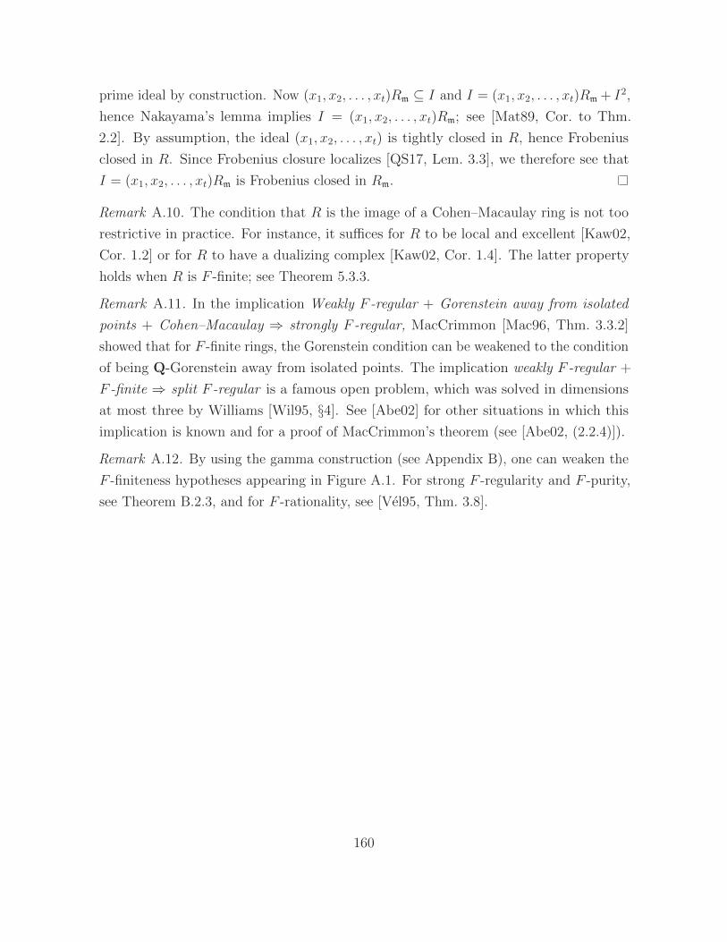
prime ideal by construction. Now (x1, x2, . . . , xt)Rm ⊆ I and I = (x1, x2, . . . , xt)Rm + I2,

hence Nakayama’s lemma implies I = (x1, x2, . . . , xt)Rm; see [Mat89, Cor. to Thm.

2.2]. By assumption, the ideal (x1, x2, . . . , xt) is tightly closed in R, hence Frobenius

closed in R. Since Frobenius closure localizes [QS17, Lem. 3.3], we therefore see that

I = (x1, x2, . . . , xt)Rm is Frobenius closed in Rm.

Remark A.10. The condition that R is the image of a Cohen–Macaulay ring is not too

restrictive in practice. For instance, it suffices for R to be local and excellent [Kaw02,

Cor. 1.2] or for R to have a dualizing complex [Kaw02, Cor. 1.4]. The latter property

holds when R is F -finite; see Theorem 5.3.3.

Remark A.11. In the implication Weakly F -regular + Gorenstein away from isolated

points + Cohen–Macaulay ⇒ strongly F -regular, MacCrimmon [Mac96, Thm. 3.3.2]

showed that for F -finite rings, the Gorenstein condition can be weakened to the condition

of being Q-Gorenstein away from isolated points. The implication weakly F -regular +

F -finite ⇒ split F -regular is a famous open problem, which was solved in dimensions

at most three by Williams [Wil95, §4]. See [Abe02] for other situations in which this

implication is known and for a proof of MacCrimmon’s theorem (see [Abe02, (2.2.4)]).

Remark A.12. By using the gamma construction (see Appendix B), one can weaken the

F -finiteness hypotheses appearing in Figure A.1. For strong F -regularity and F -purity,

see Theorem B.2.3, and for F -rationality, see [Vel95, Thm. 3.8].

160

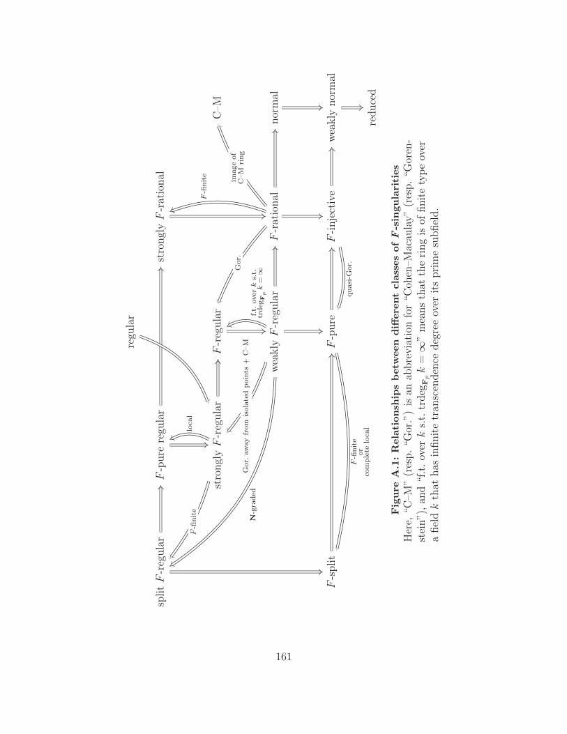
regu

lar

splitF

-reg

ula

rF

-pure

regu

lar

stro

ngl

yF

-rat

ional

stro

ngl

yF

-reg

ula

rF

-reg

ula

rC

–M

wea

klyF

-reg

ula

rF

-rat

ional

nor

mal

F-s

plit

F-p

ure

F-i

nje

ctiv

ew

eakly

nor

mal

reduce

d

loca

lF

-fin

ite

N-g

rad

edG

or.

aw

ay

from

isola

ted

poin

ts+

C–M

f.t.

overk

s.t.

trd

egF

pk

=∞G

or.

F-fi

nit

e

image

of

C–M

rin

g

F-fi

nit

eor

com

ple

telo

cal

qu

asi

-Gor.

Fig

ure

A.1

:R

ela

tion

ship

sb

etw

een

diff

ere

nt

cla

sses

ofF

-sin

gu

lari

ties

Her

e,“C

–M”

(res

p.

“Gor

.”)

isan

abb

revia

tion

for

“Coh

en–M

acau

lay”

(res

p.

“Gor

en-

stei

n”)

,an

d“f

.t.

overk

s.t.

trdeg

Fpk

=∞

”m

ean

sth

atth

eri

ng

isof

fin

ite

typ

eov

era

fiel

dk

that

has

infinit

etr

ansc

enden

cedeg

ree

over

its

pri

me

subfiel

d.

161

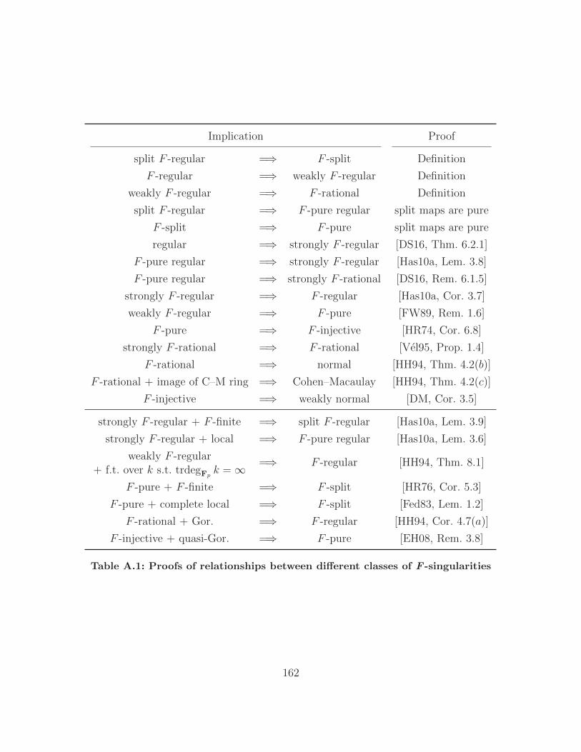
Implication Proof

split F -regular =⇒ F -split Definition

F -regular =⇒ weakly F -regular Definition

weakly F -regular =⇒ F -rational Definition

split F -regular =⇒ F -pure regular split maps are pure

F -split =⇒ F -pure split maps are pure

regular =⇒ strongly F -regular [DS16, Thm. 6.2.1]

F -pure regular =⇒ strongly F -regular [Has10a, Lem. 3.8]

F -pure regular =⇒ strongly F -rational [DS16, Rem. 6.1.5]

strongly F -regular =⇒ F -regular [Has10a, Cor. 3.7]

weakly F -regular =⇒ F -pure [FW89, Rem. 1.6]

F -pure =⇒ F -injective [HR74, Cor. 6.8]

strongly F -rational =⇒ F -rational [Vel95, Prop. 1.4]

F -rational =⇒ normal [HH94, Thm. 4.2(b)]

F -rational + image of C–M ring =⇒ Cohen–Macaulay [HH94, Thm. 4.2(c)]

F -injective =⇒ weakly normal [DM, Cor. 3.5]

strongly F -regular + F -finite =⇒ split F -regular [Has10a, Lem. 3.9]

strongly F -regular + local =⇒ F -pure regular [Has10a, Lem. 3.6]

weakly F -regular+ f.t. over k s.t. trdegFp k =∞ =⇒ F -regular [HH94, Thm. 8.1]

F -pure + F -finite =⇒ F -split [HR76, Cor. 5.3]

F -pure + complete local =⇒ F -split [Fed83, Lem. 1.2]

F -rational + Gor. =⇒ F -regular [HH94, Cor. 4.7(a)]

F -injective + quasi-Gor. =⇒ F -pure [EH08, Rem. 3.8]

Table A.1: Proofs of relationships between different classes of F -singularities

162

Appendix B

The gamma construction of

Hochster–Huneke

We prove a scheme-theoretic version of the gamma construction of Hochster–Huneke

[HH94], which we use to systematically reduce questions about varieties over an arbitrary

imperfect field to the same questions over an F -finite field (that is still imperfect). In

commutative algebra, the construction was first introduced in order to prove that test

elements (in the sense of tight closure) exist for rings that are essentially of finite type

over an excellent local ring of characteristic p > 0. The material below is from [Mur].

B.1. Construction and main result

The following is the main consequence of the gamma construction:

Theorem B.1.1. Let X be a scheme essentially of finite type over a field k of char-

acteristic p > 0, and let Q be a set of properties in the following list: local complete

intersection, Gorenstein, Cohen–Macaulay, Sn, Rn, normal, weakly normal, reduced,

strongly F -regular, F -pure, F -rational, F -injective. Then, there exists a purely in-

separable field extension k ⊆ kΓ such that kΓ is F -finite and such that the projection

morphism

πΓ : X ×k kΓ −→ X

is a homeomorphism that identifies P loci for every P ∈ Q.

163

Here, we recall that for a scheme X and a property P of local rings on X, the P locus

of X is

P(X) :=x ∈ X

∣∣ OX,x is P.

We will in fact show a more general result (Theorem B.1.6), which allows for k to be

replaced by a complete local ring, and allows finitely many schemes instead of just one.

Note that Theorem B.1.1 for weak normality, F -purity, and F -injectivity are new even

in the affine setting.

Before describing the construction, we motivate the idea behind the construction with

the following:

Example B.1.2. Let k be a non-F -finite field of characteristic p > 2, and let a ∈k r kp. For example, we can let k = Fp(xi)i∈N and let a = x0. Let S = k[x, y] and

f = y2 + xp − a ∈ S, and consider Chevalley’s example [Zar47, Ex. 3]

R = S/(f) =k[x, y]

y2 + xp − a.

We claim that R is regular. Note that R is smooth everywhere except at the maximal

ideal (xp − a, y), since the Jacobian for R is (0, 2y). It therefore suffices to show that R

is regular at mR := (xp − a, y)R ⊆ R. To avoid confusion, we denote by mS the ideal

(xp − a, y)S ⊆ S. We have

dimS/mS

(mS

m2S

)= 2,

since S is regular. On the other hand, the defining equation f = y2 + xp − a for R is

nonzero modulo m2S, hence

dimR/mR

(mR

m2R

)= dimS/mS

(mS

m2S + (f)

)= 1.

Thus, RmR is regular, and R is regular everywhere.

We would now like to find a field extension k ⊆ k′ such that R⊗k k′ is F -finite and

regular. First, we claim that setting k′ = kperf will result in an F -finite ring that is not

regular. Set

R′ := R⊗k k(a1/p) ' k(a1/p)[x, y]

y2 + xp − a 'k(a1/p)[x, y]

y2 + (x− a1/p)p,

164

and denote mR′ = (x− a1/p, y)R′. We have that

y2 + xp − a = y2 + (x− a1/p)2 · (x− a1/p)2−p ∈ (x− a1/p, y)2,

hence

dimR′/mR′

(mR′

m2R′

)= dimS/mS

(mS

m2S + (f)

)= 2.

Thus, we see that R′ is not regular at the maximal ideal mR′ . We therefore want to

find a field extension k ⊆ k′ that avoids adjoining a1/p, such that k′ is still F -finite.

The gamma construction (Theorem B.1.1) ensures the existence of such an extension,

although we note that in the specific case where k = Fp(xi)i∈N and a = x0 above, we

can set k′ = Fp(x0)(xi)i∈Nr0.

We now give an account of Hochster and Huneke’s construction.

Construction B.1.3 [HH94, (6.7) and (6.11)]. Let (A,m, k) be a noetherian complete

local ring of characteristic p > 0. By the Cohen structure theorem, we may identify k

with a coefficient field k ⊆ A. Moreover, by Zorn’s lemma (see [Mat89, p. 202]), we may

choose a p-basis Λ for k, which is a subset Λ ⊆ k such that k = kp(Λ), and such that for

every finite subset Σ ⊆ Λ with s elements, we have [kp(Σ) : kp] = ps.

Now let Γ ⊆ Λ be a cofinite subset, i.e., a subset Γ of Λ such that Λ r Γ is a finite

set. For each integer e ≥ 0, consider the subfield kΓe = k[λ1/pe ]λ∈Γ ⊆ kperf of some perfect

closure kperf of k. These form an ascending chain, and we then set

AΓ := lim−→e

kΓe JAK,

where kΓe JAK is the completion of kΓ

e ⊗k A at the extended ideal m · (kΓe ⊗k A). Note that

if A = k is a field, then AΓ = kΓ is a field by construction.

Finally, let X be a scheme essentially of finite type over A, and consider two cofinite

subsets Γ ⊆ Λ and Γ′ ⊆ Λ such that Γ ⊆ Γ′. We then have the following commutative

165

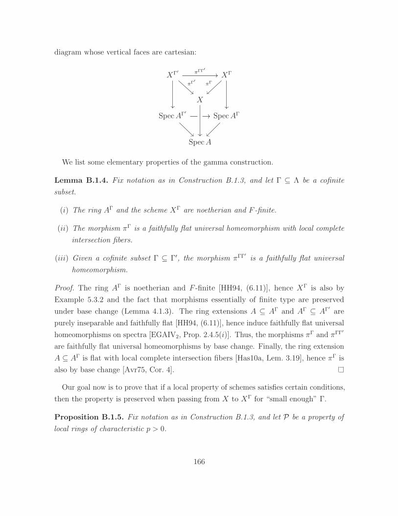
diagram whose vertical faces are cartesian:

XΓ′ XΓ

X

SpecAΓ′ SpecAΓ

SpecA

πΓ′

πΓΓ′

πΓ

We list some elementary properties of the gamma construction.

Lemma B.1.4. Fix notation as in Construction B.1.3, and let Γ ⊆ Λ be a cofinite

subset.

(i) The ring AΓ and the scheme XΓ are noetherian and F -finite.

(ii) The morphism πΓ is a faithfully flat universal homeomorphism with local complete

intersection fibers.

(iii) Given a cofinite subset Γ ⊆ Γ′, the morphism πΓΓ′ is a faithfully flat universal

homeomorphism.

Proof. The ring AΓ is noetherian and F -finite [HH94, (6.11)], hence XΓ is also by

Example 5.3.2 and the fact that morphisms essentially of finite type are preserved

under base change (Lemma 4.1.3). The ring extensions A ⊆ AΓ and AΓ ⊆ AΓ′ are

purely inseparable and faithfully flat [HH94, (6.11)], hence induce faithfully flat universal

homeomorphisms on spectra [EGAIV2, Prop. 2.4.5(i)]. Thus, the morphisms πΓ and πΓΓ′

are faithfully flat universal homeomorphisms by base change. Finally, the ring extension

A ⊆ AΓ is flat with local complete intersection fibers [Has10a, Lem. 3.19], hence πΓ is

also by base change [Avr75, Cor. 4].

Our goal now is to prove that if a local property of schemes satisfies certain conditions,

then the property is preserved when passing from X to XΓ for “small enough” Γ.

Proposition B.1.5. Fix notation as in Construction B.1.3, and let P be a property of

local rings of characteristic p > 0.

166

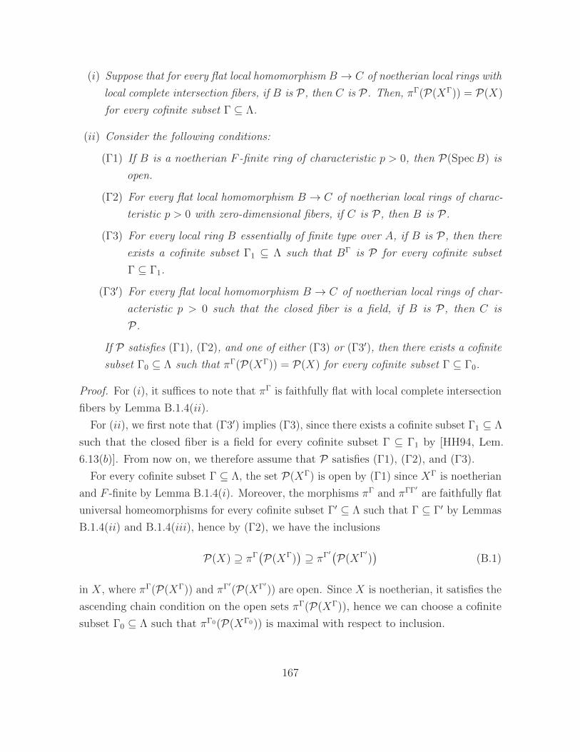
(i) Suppose that for every flat local homomorphism B → C of noetherian local rings with

local complete intersection fibers, if B is P, then C is P. Then, πΓ(P(XΓ)) = P(X)

for every cofinite subset Γ ⊆ Λ.

(ii) Consider the following conditions:

(Γ1) If B is a noetherian F -finite ring of characteristic p > 0, then P(SpecB) is

open.

(Γ2) For every flat local homomorphism B → C of noetherian local rings of charac-

teristic p > 0 with zero-dimensional fibers, if C is P, then B is P.

(Γ3) For every local ring B essentially of finite type over A, if B is P, then there

exists a cofinite subset Γ1 ⊆ Λ such that BΓ is P for every cofinite subset

Γ ⊆ Γ1.

(Γ3′) For every flat local homomorphism B → C of noetherian local rings of char-

acteristic p > 0 such that the closed fiber is a field, if B is P, then C is

P.

If P satisfies (Γ1), (Γ2), and one of either (Γ3) or (Γ3′), then there exists a cofinite

subset Γ0 ⊆ Λ such that πΓ(P(XΓ)) = P(X) for every cofinite subset Γ ⊆ Γ0.

Proof. For (i), it suffices to note that πΓ is faithfully flat with local complete intersection

fibers by Lemma B.1.4(ii).

For (ii), we first note that (Γ3′) implies (Γ3), since there exists a cofinite subset Γ1 ⊆ Λ

such that the closed fiber is a field for every cofinite subset Γ ⊆ Γ1 by [HH94, Lem.

6.13(b)]. From now on, we therefore assume that P satisfies (Γ1), (Γ2), and (Γ3).

For every cofinite subset Γ ⊆ Λ, the set P(XΓ) is open by (Γ1) since XΓ is noetherian

and F -finite by Lemma B.1.4(i). Moreover, the morphisms πΓ and πΓΓ′ are faithfully flat

universal homeomorphisms for every cofinite subset Γ′ ⊆ Λ such that Γ ⊆ Γ′ by Lemmas

B.1.4(ii) and B.1.4(iii), hence by (Γ2), we have the inclusions

P(X) ⊇ πΓ(P(XΓ)

)⊇ πΓ′

(P(XΓ′)

)(B.1)

in X, where πΓ(P(XΓ)) and πΓ′(P(XΓ′)) are open. Since X is noetherian, it satisfies the

ascending chain condition on the open sets πΓ(P(XΓ)), hence we can choose a cofinite

subset Γ0 ⊆ Λ such that πΓ0(P(XΓ0)) is maximal with respect to inclusion.

167

We claim that P(X) = πΓ0(P(XΓ0)) for every cofinite subset Γ ⊆ Γ0. By (B.1),

it suffices to show the inclusion ⊆. Suppose there exists x ∈ P(X) r πΓ0(P(XΓ0)).

By (Γ3), there exists a cofinite subset Γ1 ⊆ Λ such that (πΓ)−1(x) ∈ P(XΓ) for every

cofinite subset Γ ⊆ Γ1. Choosing Γ = Γ0 ∩ Γ1, we have x ∈ πΓ(P(XΓ)) r πΓ0(P(XΓ0)),

contradicting the maximality of πΓ0(P(XΓ0)).

We now prove that the properties in Theorem B.1.1 are preserved when passing to

XΓ. Special cases of the following result appear in [HH94, Lem. 6.13], [Vel95, Thm. 2.2],

[EH08, Lem. 2.9], [Has10a, Lems. 3.23 and 3.30], and [Ma14, Prop. 5.6].

Theorem B.1.6. Fix notation as in Construction B.1.3.

(i) For every cofinite subset Γ ⊆ Λ, the map πΓ identifies local complete intersection,

Gorenstein, Cohen–Macaulay, and Sn loci.

(ii) There exists a cofinite subset Γ0 ⊆ Λ such that πΓ identifies Rn (resp. normal,

weakly normal, reduced, strongly F -regular, F -pure, F -rational, F -injective) loci

for every cofinite subset Γ ⊆ Γ0.

Note that Theorem B.1.6 implies Theorem B.1.1 since if A is a field, then AΓ is also

by Construction B.1.3, and moreover if one wants to preserve more than one property at

once, then it suffices to intersect the various Γ0 for the different properties.

Proof. For (i), it suffices to note that these properties satisfy the condition in Proposition

B.1.5(i) by [Avr75, Cor. 2] and [Mat89, Thm. 23.4, Cor. to Thm. 23.3, and Thm.

23.9(iii)], respectively.

We now prove (ii). We first note that (ii) holds for regularity since (Γ1) holds by the

excellence of XΓ, and (Γ2) and (Γ3′) hold by [Mat89, Thm. 23.7]. Since πΓ preserves

the dimension of local rings, we therefore see that (ii) holds for Rn. (ii) for normality

and reducedness then follows from (i) since they are equivalent to R1 + S2 and R0 + S1,

respectively.

To prove (ii) holds in the remaining cases, we check the conditions in Proposition

B.1.5(ii). For weak normality, (Γ1) holds by [BF93, Thm. 7.1.3], and (Γ2) holds by

[Man80, Cor. II.2]. To show that (Γ3) holds, recall by [Man80, Thm. I.6] that a reduced

ring B is weakly normal if and only if

B Bν (Bν ⊗B Bν)red

b7→b⊗1

b7→1⊗b(B.2)

168

is an equalizer diagram, where Bν is the normalization of B. Now suppose B is weakly

normal, and let Γ1 ⊆ Λ be a cofinite subset such that BΓ is reduced, (Bν)Γ is normal,

and ((Bν ⊗B Bν)red)Γ is reduced for every cofinite subset Γ ⊆ Γ1; such a Γ1 exists by the

previous paragraph. We claim that BΓ is weakly normal for every Γ ⊆ Γ1 cofinite in Λ.

Since (B.2) is an equalizer diagram and A ⊆ AΓ is flat, the diagram

BΓ (Bν)Γ((Bν ⊗B Bν)red

)Γb 7→b⊗1

b 7→1⊗b

is an equalizer diagram. Moreover, since BΓ ⊆ (Bν)Γ is an integral extension of rings

with the same total ring of fractions, and (Bν)Γ is normal, we see that (Bν)Γ = (BΓ)ν .

Finally, ((Bν ⊗B Bν)red)Γ is reduced, hence we have the natural isomorphism

((Bν ⊗B Bν)red

)Γ '((BΓ)ν ⊗BΓ (BΓ)ν

)red.

Thus, since the analogue of (B.2) with B replaced by BΓ is an equalizer diagram, we

see that BΓ is weakly normal for every Γ ⊆ Γ1 cofinite in Λ, hence (Γ3) holds for weak

normality.

We now prove (ii) for strong F -regularity, F -purity, and F -rationality. First, (Γ1)

holds for strong F -regularity by [Has10a, Lem. 3.29], and the same argument shows

that (Γ1) holds for F -purity since the F -pure and F -split loci coincide for F -finite rings

[HR76, Cor. 5.3]. Next, (Γ1) for F -rationality holds by [Vel95, Thm. 1.11] since the

reduced locus is open and reduced F -finite rings are admissible in the sense of [Vel95,

Def. 1.5] by Theorem 5.3.3. It then suffices to note that (Γ2) holds by [Has10a, Lem.

3.17], [HR76, Prop. 5.13], and [Vel95, (6) on p. 440], respectively, and (Γ3) holds by

[Has10a, Cor. 3.31], [Ma14, Prop. 5.4], and [Vel95, Lem. 2.3], respectively.

Finally, we prove (ii) for F -injectivity. First, (Γ1) and (Γ2) hold by [Mur, Lem. A.2]

and [Mur, Lem. A.3], respectively. The proof of [EH08, Lem. 2.9(b)] implies (Γ3), since

the residue field of B is a finite extension of k, hence socles of artinian B-modules are

finite-dimensional k-vector spaces.

169

B.2. Applications

We now give some applications of the gamma construction (Theorem B.1.6). See also

[Mur, §3.2] for applications to the minimal model program over imperfect fields.

B.2.1. Openness of F -singularities

We have the following consequence of Theorem B.1.6, which was first attributed to Hoshi

in [Has10b, Thm. 3.2]. Note that the analogous statements for strong F -regularity and

F -rationality appear in [Has10a, Prop. 3.33] and [Vel95, Thm. 3.5], respectively.

Corollary B.2.1. Let X be a scheme essentially of finite type over a local G-ring (A,m)

of characteristic p > 0. Then, the F -pure locus is open in X.

Recall that a noetherian ring R is a G-ring if, for every prime ideal p ⊆ R, the

completion homomorphisms Rp → Rp are regular in the sense of [EGAIV2, Def. 6.8.1].

Proof. Let A→ A be the completion of A at m, and let Λ be a p-basis for A/mA as in

Construction B.1.3. For every cofinite subset Γ ⊆ Λ, consider the commutative diagram

X ×A AΓ X ×A A X

Spec AΓ Spec A SpecA

πΓ π

where the squares are cartesian. By Theorem B.1.6, there exists a cofinite subset Γ ⊆ Λ

such that πΓ is a homeomorphism identifying F -pure loci. Since X ×A AΓ is F -finite,

the F -pure locus in X ×A A is therefore open by the fact that (Γ1) holds for F -purity;

see the proof of Theorem B.1.6(ii).

Now let x ∈ X ×A A. Since A → A is a regular homomorphism, the morphism π

is also regular by base change [EGAIV2, Prop. 6.8.3(iii)]. Thus, OX×AA,x is F -pure

if and only if OX,π(x) is F -pure by [HR76, Prop. 5.13] and [Has10a, Props. 2.4(4) and

2.4(6)]. Denoting the F -pure locus in X by W , we see that π−1(W ) is the F -pure locus

in X ×A A. Since π−1(W ) is open and π is quasi-compact and faithfully flat by base

change, the F -pure locus W ⊆ X is open by [EGAIV2, Cor. 2.3.12].

170

Remark B.2.2. Although [Mur, Lem. A.2] shows that the F -injective locus is open under

F -finiteness hypotheses, and the gamma construction (Theorem B.1.6) implies that the

F -injective locus is open for schemes essentially of finite type over complete local rings,

the fact that the F -injective locus is open under the hypotheses of Corollary B.2.1 is a

recent result due to Rankeya Datta and the author [DM, Thm. B].

B.2.2. F -singularities for rings essentially of finite type

We finally show that for rings to which the gamma construction applies, the notions of

strong F -regularity and split F -regularity coincide, as do the notions of F -purity and

F -splitting. This result is unpublished work of Rankeya Datta and the author.

Theorem B.2.3. Let R be a ring essentially of finite type over a noetherian complete

local ring (A,m, k) of characteristic p > 0. If R is strongly F -regular (resp. F -pure),

then R is split F -regular (resp. F -split).

We first show the following preliminary result, which was communicated to Hochster

by Auslander (although it may be older).

Lemma B.2.4 (cf. [Fed83, Lem. 1.2]). Let (A,m, k) be a noetherian complete local ring.

Then, every pure ring homomorphism A→ B splits as an A-module homomorphism.

Proof. Let f : A → B be a pure ring homomorphism. We claim we have the follow-

ing commutative diagram with exact rows, where the vertical homomorphisms are

isomorphisms:

HomA

(B ⊗A EA(k), EA(k)

)HomA

(A⊗A EA(k), EA(k)

)0

HomA

(B,HomA

(EA(k), EA(k)

))HomA

(A,HomA

(EA(k), EA(k)

))0

HomA(B,A) HomA(A,A) 0

(f⊗idEA(k))∗

∼ ∼

f∗

f∗

∼ ∼

The top row is the Matlis dual of the map f ⊗ idEA(k) : A ⊗A EA(k) → B ⊗A EA(k),

and the second row is obtained from the first by tensor-hom adjunction. The last

row is obtained from the isomorphism HomA(EA(k), EA(k)) ' A, which holds by the

171

completeness of A [Mat89, Thm. 18.6(iv)]. Since the last row is surjective, we can choose

g ∈ HomA(B,A) such that f ∗(g) = g f = idA.

We can now show Theorem B.2.3.

Proof of Theorem B.2.3. By the gamma construction (Theorem B.1.6), there exists a

faithfully flat ring extension A → AΓ such that RΓ := R ⊗A AΓ is strongly F -regular

(resp. F -pure) and F -finite. By F -finiteness, the ring RΓ is split F -regular by [Has10a,

Lem. 3.9] (resp. F -split by [HR76, Cor. 5.3]). Now consider the commutative diagram

A R F e∗R F e

∗R

AΓ RΓ F e∗R

Γ F e∗R

Γ

F eR F e∗ (−·c)

F eRΓ F e∗ (−·(c⊗1))

for every c ∈ R and every integer e > 0, where the left square is cocartesian. Note that

if c ∈ R, then c⊗ 1 ∈ (RΓ), since R→ RΓ satisfies going-down [Mat89, Thm. 9.5].

Since the inclusion A → AΓ is faithfully flat, it is pure, hence splits as an A-module

homomorphism by Lemma B.2.4. By base change, this implies the inclusion R → RΓ

splits as an R-module homomorphism. For both split F -regularity and F -splitting, it

then suffices to note that if F e∗ (− · (c ⊗ 1)) F e

RΓ splits for some c ∈ R and for some

e > 0, then composing this splitting with a splitting of R → RΓ gives a splitting of

F e∗ (− · c) F e

R by the commutativity of the diagram above.

172

Bibliography

[Abe02] I. M. Aberbach. “Some conditions for the equivalence of weak and strong F -regularity.” Comm. Algebra 30.4 (2002), pp. 1635–1651. doi: 10.1081/AGB-120013205. mr: 1894033. 160

[AE05] I. M. Aberbach and F. Enescu. “The structure of F-pure rings.” Math.Z. 250.4 (2005), pp. 791–806. doi: 10.1007/s00209-005-0776-y. mr:2180375. 143

[AS95] U. Angehrn and Y. T. Siu. “Effective freeness and point separation foradjoint bundles.” Invent. Math. 122.2 (1995), pp. 291–308. doi: 10.1007/BF01231446. mr: 1358978. 7, 8, 16, 138

[Avr75] L. L. Avramov. “Flat morphisms of complete intersections.” Translatedfrom the Russian by D. L. Johnson. Soviet Math. Dokl. 16.6 (1975),pp. 1413–1417. mr: 396558. 166, 168

[Ax68] J. Ax. “The elementary theory of finite fields.” Ann. of Math. (2) 88 (1968),pp. 239–271. doi: 10.2307/1970573. mr: 229613. 6

[Bau99] Th. Bauer. “Seshadri constants on algebraic surfaces.” Math. Ann. 313.3(1999), pp. 547–583. doi: 10.1007/s002080050272. mr: 1678549. 22

[BB11] M. Blickle and G. Bockle. “Cartier modules: finiteness results.” J. ReineAngew. Math. 661 (2011), pp. 85–123. doi: 10.1515/CRELLE.2011.087.mr: 2863904. 128

[BBP13] S. Boucksom, A. Broustet, and G. Pacienza. “Uniruledness of stable baseloci of adjoint linear systems via Mori theory.” Math. Z. 275.1-2 (2013),pp. 499–507. doi: 10.1007/s00209-013-1144-y. mr: 3101817. 57

[BDRH+09] Th. Bauer, S. Di Rocco, B. Harbourne, M. Kapustka, A. Knutsen, W.Syzdek, and T. Szemberg. “A primer on Seshadri constants.” Interactionsof classical and numerical algebraic geometry. Contemp. Math., Vol. 496.Providence, RI: Amer. Math. Soc., 2009, pp. 33–70. doi: 10.1090/conm/496/09718. mr: 2555949. 17

173

[BF93] J. Bingener and H. Flenner. “On the fibers of analytic mappings.” Complexanalysis and geometry. Univ. Ser. Math. New York: Plenum, 1993, pp. 45–101. doi: 10.1007/978-1-4757-9771-8_2. mr: 1211878. 168

[BGGJ+] J. I. Burgos Gil, W. Gubler, P. Jell, K. Kunnemann, and F. Martin.“Differentiability of non-archimedean volumes and non-archimedean Monge-Ampere equations.” With an appendix by R. Lazarsfeld. Mar. 11, 2019.arXiv:1608.01919v6 [math.AG]. To appear in Algebraic Geometry. 50,59–61

[Bir16] C. Birkar. “Existence of flips and minimal models for 3-folds in char p.”Ann. Sci. Ec. Norm. Super. (4) 49.1 (2016), pp. 169–212. doi: 10.24033/asens.2279. mr: 3465979. 57

[Bir17] C. Birkar. “The augmented base locus of real divisors over arbitrary fields.”Math. Ann. 368.3-4 (2017), pp. 905–921. doi: 10.1007/s00208-016-1441-y. mr: 3673639. 57

[BK05] M. Brion and S. Kumar. Frobenius splitting methods in geometry andrepresentation theory. Progr. Math., Vol. 231. Boston, MA: BirkhauserBoston, Inc., 2005. doi: 10.1007/b137486. mr: 2107324. 26

[BMS08] M. Blickle, M. Mustata, and K. E. Smith. “Discreteness and rationality ofF -thresholds.” Michigan Math. J. 57 (2008): Special volume in honor ofMelvin Hochster, pp. 43–61. doi: 10.1307/mmj/1220879396. mr: 2492440.73, 86

[BS09] Th. Bauer and T. Szemberg. “Seshadri constants and the generation ofjets.” J. Pure Appl. Algebra 213.11 (2009), pp. 2134–2140. doi: 10.1016/j.jpaa.2009.03.005. mr: 2533311. 36, 40, 41, 43

[BST12] M. Blickle, K. Schwede, and K. Tucker. “F -signature of pairs and theasymptotic behavior of Frobenius splittings.” Adv. Math. 231.6 (2012),pp. 3232–3258. doi: 10.1016/j.aim.2012.09.007. mr: 2980498. 144

[CHSW16] E. Canton, D. J. Hernandez, K. Schwede, and E. E. Witt. “On the behaviorof singularities at the F -pure threshold.” With an appendix by A. DeStefani, J. Jeffries, Z. Kadyrsizova, R. M. Walker, and G. Whelan. IllinoisJ. Math. 60.3-4 (2016), pp. 669–685. doi: 10.1215/ijm/1506067286. mr:3705442. 81

[CMSB02] K. Cho, Y. Miyaoka, and N. I. Shepherd-Barron. “Characterizations ofprojective space and applications to complex symplectic manifolds.” Higherdimensional birational geometry (Kyoto, 1997). Adv. Stud. Pure Math.,Vol. 35. Tokyo: Math. Soc. Japan, 2002, pp. 1–88. doi: 10.2969/aspm/03510001. mr: 1929792. 38, 39

174

[CN14] P. Cascini and M. Nakamaye. “Seshadri constants on smooth threefolds.”Adv. Geom. 14.1 (2014), pp. 59–79. doi: 10.1515/advgeom-2013-0012.mr: 3159092. 22

[Con00] B. Conrad. Grothendieck duality and base change. Lecture Notes in Math.,Vol. 1750. Berlin: Springer-Verlag, 2000. doi: 10.1007/b75857. mr: 1804902. 52

[CRST] J. Carvajal-Rojas, K. Schwede, and K. Tucker. “Bertini theorems for F -signature and Hilbert-Kunz multiplicity.” Oct. 19, 2018. arXiv:1710.

01277v2 [math.AG]. 144

[CTX15] P. Cascini, H. Tanaka, and C. Xu. “On base point freeness in positivecharacteristic.” Ann. Sci. Ec. Norm. Super. (4) 48.5 (2015), pp. 1239–1272.doi: 10.24033/asens.2269. mr: 3429479. 77

[Cut15] S. D. Cutkosky. “Teissier’s problem on inequalities of nef divisors.” J.Algebra Appl. 14.9 (2015), 1540002, 37 pp. doi: 10.1142/S0219498815400022. mr: 3368254. 99

[dC98] M. A. A. de Cataldo. “Effective nonvanishing, effective global generation.”Ann. Inst. Fourier (Grenoble) 48.5 (1998), pp. 1359–1378. doi: 10.5802/aif.1658. mr: 1662243. 23

[DCF15] G. Di Cerbo and A. Fanelli. “Effective Matsusaka’s theorem for surfaces incharacteristic p.” Algebra Number Theory 9.6 (2015), pp. 1453–1475. doi:10.2140/ant.2015.9.1453. mr: 3397408. 4, 16

[Deb] O. Debarre. “Cohomological characterizations of the complex projectivespace.” Dec. 14, 2015. arXiv:1512.04321v1 [math.AG]. 41

[DEL00] J.-P. Demailly, L. Ein, and R. Lazarsfeld. “A subadditivity property ofmultiplier ideals.” Michigan Math. J. 48 (2000): Dedicated to WilliamFulton on the occasion of his 60th birthday, pp. 137–156. doi: 10.1307/mmj/1030132712. mr: 1786484. 67

[Dem92] J.-P. Demailly. “Singular Hermitian metrics on positive line bundles.”Complex algebraic varieties (Bayreuth, 1990). Lecture Notes in Math.,Vol. 1507. Berlin: Springer-Verlag, 1992, pp. 87–104. doi: 10.1007/BFb0094512. mr: 1178721. 4, 18, 19

[Den] Y. Deng. “Applications of the Ohsawa-Takegoshi extension theorem todirect image problems.” Oct. 23, 2017. arXiv:1703.07279v2 [math.AG].Submitted. 24

[dFKL07] T. de Fernex, A. Kuronya, and R. Lazarsfeld. “Higher cohomology ofdivisors on a projective variety.” Math. Ann. 337.2 (2007), pp. 443–455.doi: 10.1007/s00208-006-0044-4. mr: 2262793. 9, 96, 97, 99, 107, 108

175

[dFM09] T. de Fernex and M. Mustata. “Limits of log canonical thresholds.” Ann.Sci. Ec. Norm. Super. (4) 42.3 (2009), pp. 491–515. doi: 10.24033/asens.2100. mr: 2543330. 66, 67, 105

[dJ96] A. J. de Jong. “Smoothness, semi-stability and alterations.” Inst. HautesEtudes Sci. Publ. Math. 83 (1996), pp. 51–93. doi: 10.1007/BF02698644.mr: 1423020. 24, 61, 101

[DM] R. Datta and T. Murayama. “On the behavior of F -injectivity under flathomomorphisms.” In preparation. 155, 162, 171

[DM19] Y. Dutta and T. Murayama. “Effective generation and twisted weak posi-tivity of direct images.” Algebra Number Theory 13.2 (2019), pp. 425–454.doi: 10.2140/ant.2019.13.425. 23, 24

[DRS01] S. Di Rocco and A. J. Sommese. “Line bundles for which a projectivized jetbundle is a product.” Proc. Amer. Math. Soc. 129.6 (2001), pp. 1659–1663.doi: 10.1090/S0002-9939-00-05875-5. mr: 1814094. 42

[DS16] R. Datta and K. E. Smith. “Frobenius and valuation rings.” Algebra NumberTheory 10.5 (2016), pp. 1057–1090. doi: 10.2140/ant.2016.10.1057. mr:3531362. See also [DS17]. 155, 157, 162

[DS17] R. Datta and K. E. Smith. “Correction to the article “Frobenius andvaluation rings”.” Algebra Number Theory 11.4 (2017), pp. 1003–1007. doi:10.2140/ant.2017.11.1003. mr: 3665644. 176

[DSNB18] A. De Stefani and L. Nunez-Betancourt. “F -thresholds of graded rings.”Nagoya Math. J. 229 (2018), pp. 141–168. doi: 10.1017/nmj.2016.65.mr: 3778235. 144

[Dut] Y. Dutta. “On the effective freeness of the direct images of pluricanonicalbundles.” Oct. 27, 2018. arXiv:1701.08830v4 [math.AG]. Submitted. 24

[EGAInew] A. Grothendieck and J. Dieudonne. Elements de geometrie algebrique. I.Le langage des schemas. New edition. Grundlehren Math. Wiss., Vol. 166.Berlin: Springer-Verlag, 1971. mr: 3075000. 47, 48

[EGAII] A. Grothendieck and J. Dieudonne. “Elements de geometrie algebrique. II.Etude globale elementaire de quelques classes de morphismes.” Inst. HautesEtudes Sci. Publ. Math. 8 (1961), pp. 1–222. doi: 10.1007/BF02699291.mr: 163909. 14

[EGAIII2] A. Grothendieck and J. Dieudonne. “Elements de geometrie algebrique. III.Etude cohomologique des faisceaux coherents. II.” Inst. Hautes Etudes Sci.Publ. Math. 17 (1963), pp. 1–91. doi: 10.1007/BF02684890. mr: 163911.135

176

[EGAIV1] A. Grothendieck and J. Dieudonne. “Elements de geometrie algebrique. IV.Etude locale des schemas et des morphismes de schemas. I.” Inst. HautesEtudes Sci. Publ. Math. 20 (1964), pp. 1–259. doi: 10.1007/BF02684747.mr: 173675. 46–48, 92

[EGAIV2] A. Grothendieck and J. Dieudonne. “Elements de geometrie algebrique. IV.Etude locale des schemas et des morphismes de schemas. II.” Inst. HautesEtudes Sci. Publ. Math. 24 (1965), pp. 1–231. doi: 10.1007/BF02684890.mr: 199181. 69, 100, 135, 136, 140, 148, 166, 170

[EGAIV3] A. Grothendieck and J. Dieudonne. “Elements de geometrie algebrique. IV.Etude locale des schemas et des morphismes de schemas. III.” Inst. HautesEtudes Sci. Publ. Math. 28 (1966), pp. 1–255. doi: 10.1007/BF02684343.mr: 217086. 6, 89–93, 107, 108

[EGAIV4] A. Grothendieck and J. Dieudonne. “Elements de geometrie algebrique. IV.Etude locale des schemas et des morphismes de schemas. IV.” Inst. HautesEtudes Sci. Publ. Math. 32 (1967), pp. 1–361. doi: 10.1007/BF02732123.mr: 238860. 41, 49, 50, 91

[EH08] F. Enescu and M. Hochster. “The Frobenius structure of local cohomology.”Algebra Number Theory 2.7 (2008), pp. 721–754. doi: 10.2140/ant.2008.2.721. mr: 2460693. 162, 168, 169

[EKL95] L. Ein, O. Kuchle, and R. Lazarsfeld. “Local positivity of ample linebundles.” J. Differential Geom. 42.2 (1995), pp. 193–219. doi: 10.4310/jdg/1214457231. mr: 1366545. 22, 40

[EL93a] L. Ein and R. Lazarsfeld. “Global generation of pluricanonical and adjointlinear series on smooth projective threefolds.” J. Amer. Math. Soc. 6.4(1993), pp. 875–903. doi: 10.2307/2152744. mr: 1207013. 4, 16

[EL93b] L. Ein and R. Lazarsfeld. “Seshadri constants on smooth surfaces.” As-terisque 218 (1993): Journees de geometrie algebrique d’Orsay (Orsay,1992), pp. 177–186. url: http://www.numdam.org/item/AST_1993__218__177_0/. mr: 1265313. 13, 20–22

[ELM+05] L. Ein, R. Lazarsfeld, M. Mustata, M. Nakamaye, and M. Popa. “Asymp-totic invariants of line bundles.” Pure Appl. Math. Q. 1.2 (2005): Specialissue: In memory of Armand Borel. Part 1, pp. 379–403. doi: 10.4310/PAMQ.2005.v1.n2.a8. mr: 2194730. 55, 98

[ELM+06] L. Ein, R. Lazarsfeld, M. Mustata, M. Nakamaye, and M. Popa. “Asymp-totic invariants of base loci.” Ann. Inst. Fourier (Grenoble) 56.6 (2006),pp. 1701–1734. doi: 10.5802/aif.2225. mr: 2282673. 56–59, 119, 120

177

[ELM+09] L. Ein, R. Lazarsfeld, M. Mustata, M. Nakamaye, and M. Popa. “Restrictedvolumes and base loci of linear series.” Amer. J. Math. 131.3 (2009), pp. 607–651. doi: 10.1353/ajm.0.0054. mr: 2530849. 8, 18, 61, 111–113, 115,121–123

[Fed83] R. Fedder. “F -purity and rational singularity.” Trans. Amer. Math. Soc.278.2 (1983), pp. 461–480. doi: 10.2307/1999165. mr: 701505. 157, 162,171

[FMa] M. Fulger and T. Murayama. “Seshadri constants for vector bundles.”Mar. 5, 2019. arXiv:1903.00610v2 [math.AG]. Submitted. 18, 23, 24, 57,117, 127

[FMb] M. Fulger and T. Murayama. “Moving Seshadri constants for vector bun-dles.” In preparation. 111

[FOV99] H. Flenner, L. O’Carroll, and W. Vogel. Joins and intersections. SpringerMonogr. Math. Berlin: Springer-Verlag, 1999. doi: 10.1007/978-3-662-03817-8. mr: 1724388. 103, 107, 108

[Fra61] T. Frankel. “Manifolds with positive curvature.” Pacific J. Math. 11 (1961),pp. 165–174. doi: 10.2140/pjm.1961.11.165. mr: 123272. 37

[Fuj03] O. Fujino. “Notes on toric varieties from Mori theoretic viewpoint.” TohokuMath. J. (2) 55.4 (2003), pp. 551–564. doi: 10.2748/tmj/1113247130.mr: 2017225. 15

[Fuj11] O. Fujino. “Fundamental theorems for the log minimal model program.”Publ. Res. Inst. Math. Sci. 47.3 (2011), pp. 727–789. doi: 10.2977/PRIMS/50. mr: 2832805. 147

[Fuj18] K. Fujita. “Optimal bounds for the volumes of Kahler-Einstein Fanomanifolds.” Amer. J. Math. 140.2 (2018), pp. 391–414. doi: 10.1353/ajm.2018.0009. mr: 3783213. 125

[Fuj80] T. Fujita. “On topological characterizations of complex projective spacesand affine linear spaces.” Proc. Japan Acad. Ser. A Math. Sci. 56.5 (1980),pp. 231–234. doi: 10.3792/pjaa.56.231. mr: 580087. 41

[Fuj83] T. Fujita. “Semipositive line bundles.” J. Fac. Sci. Univ. Tokyo Sect. IAMath. 30.2 (1983), pp. 353–378. url: http://hdl.handle.net/2261/6381.mr: 722501. 30, 35, 55, 58, 126

[Fuj87] T. Fujita. “On polarized manifolds whose adjoint bundles are not semi-positive.” Algebraic geometry (Sendai, 1985). Adv. Stud. Pure Math.,Vol. 10. Amsterdam: North-Holland, 1987, pp. 167–178. doi: 10.2969/aspm/01010167. mr: 946238. 4, 14

178

[Fuj88] T. Fujita. “Problems.” Birational geometry of algebraic varieties. Openproblems (Katata, 1988). Taniguchi Foundation Division of Mathematics,1988, pp. 42–45. 4, 14

[FW89] R. Fedder and K.-i. Watanabe. “A characterization of F -regularity in termsof F -purity.” Commutative algebra (Berkeley, CA, 1987). Math. Sci. Res.Inst. Publ., Vol. 15. New York: Springer-Verlag, 1989, pp. 227–245. doi:10.1007/978-1-4612-3660-3_11. mr: 1015520. 156, 162

[Gab04] O. Gabber. “Notes on some t-structures.” Geometric aspects of Dworktheory. Vol. II. Berlin: Walter de Gruyter, 2004, pp. 711–734. doi: 10.1515/9783110198133.2.711. mr: 2099084. 74

[GW10] U. Gortz and T. Wedhorn. Algebraic geometry I. Schemes with examplesand exercises. Adv. Lectures Math. Wiesbaden: Vieweg + Teubner, 2010.doi: 10.1007/978-3-8348-9722-0. mr: 2675155. 18, 47, 91

[Har01] N. Hara. “Geometric interpretation of tight closure and test ideals.” Trans.Amer. Math. Soc. 353.5 (2001), pp. 1885–1906. doi: 10.1090/S0002-9947-01-02695-2. mr: 1813597. 94

[Har05] N. Hara. “A characteristic p analog of multiplier ideals and applications.”Comm. Algebra 33.10 (2005), pp. 3375–3388. doi: 10.1080/AGB-200060022. mr: 2175438. 87

[Har07] R. Hartshorne. “Generalized divisors and biliaison.” Illinois J. Math. 51.1(2007), pp. 83–98. doi: 10.1215/ijm/1258735326. mr: 2346188. 53

[Har66] R. Hartshorne. Residues and duality. Lecture notes of a seminar on thework of A. Grothendieck, given at Harvard 1963/64. With an appendix byP. Deligne. Lecture Notes in Math., Vol. 20. Berlin-New York: Springer-Verlag, 1966. doi: 10.1007/BFb0080482. mr: 222093. 10, 52, 53, 74, 132,158

[Har70] R. Hartshorne. Ample subvarieties of algebraic varieties. Notes written incollaboration with C. Musili. Lecture Notes in Math., Vol. 156. Berlin-NewYork: Springer-Verlag, 1970. doi: 10.1007/BFb0067839. mr: 282977. 37

[Har77] R. Hartshorne. Algebraic geometry. Grad. Texts in Math., Vol. 52. NewYork-Heidelberg: Springer-Verlag, 1977. doi: 10.1007/978-1-4757-3849-0. mr: 463157. 10–13, 15, 16, 18, 19, 29, 31, 32, 34, 35, 37, 39, 44, 51, 54,101, 102, 104, 123

[Har94] R. Hartshorne. “Generalized divisors on Gorenstein schemes.” K-Theory8.3 (1994): Proceedings of conference on algebraic geometry and ring theoryin honor of Michael Artin (Antwerp, 1992). Part III, pp. 287–339. doi:10.1007/BF00960866. mr: 1291023. 51–53, 78

179

[Has10a] M. Hashimoto. “F -pure homomorphisms, strong F -regularity, and F -injectivity.” Comm. Algebra 38.12 (2010), pp. 4569–4596. doi: 10.1080/00927870903431241. mr: 2764840. 155, 157, 158, 162, 166, 168–170, 172

[Has10b] M. Hashimoto. “F -purity of homomorphisms, strong F -regularity, and F -injectivity.” The 31st symposium on commutative algebra in Japan (Osaka,2009). 2010, pp. 9–16. url: http://www.math.okayama- u.ac.jp/

~hashimoto/paper/Comm-Alg/31-all.pdf. 170

[Hau10] H. Hauser. “On the problem of resolution of singularities in positivecharacteristic (or: a proof we are still waiting for).” Bull. Amer. Math. Soc.(N.S.) 47.1 (2010), pp. 1–30. doi: 10.1090/S0273-0979-09-01274-9. mr:2566444. 24

[Hei02] G. Heier. “Effective freeness of adjoint line bundles.” Doc. Math. 7 (2002),pp. 31–42. url: https://www.math.uni-bielefeld.de/documenta/vol-07/02.html. mr: 1911209. 16

[Hel97] S. Helmke. “On Fujita’s conjecture.” Duke Math. J. 88.2 (1997), pp. 201–216. doi: 10.1215/S0012-7094-97-08807-4. mr: 1455517. 16

[Hel99] S. Helmke. “On global generation of adjoint linear systems.” Math. Ann.313.4 (1999), pp. 635–652. doi: 10.1007/s002080050276. mr: 1686947.16

[Her12] D. J. Hernandez. “F -purity of hypersurfaces.” Math. Res. Lett. 19.2 (2012),pp. 389–401. doi: 10.4310/MRL.2012.v19.n2.a11. mr: 2955770. 77

[HH02] M. Hochster and C. Huneke. “Comparison of symbolic and ordinary powersof ideals.” Invent. Math. 147.2 (2002), pp. 349–369. doi: 10.1007/s002220100176. mr: 1881923. 28, 71

[HH90] M. Hochster and C. Huneke. “Tight closure, invariant theory, and theBriancon-Skoda theorem.” J. Amer. Math. Soc. 3.1 (1990), pp. 31–116.doi: 10.2307/1990984. mr: 1017784. 6, 81, 83, 89, 155, 156, 158

[HH94] M. Hochster and C. Huneke. “F -regularity, test elements, and smooth basechange.” Trans. Amer. Math. Soc. 346.1 (1994), pp. 1–62. doi: 10.2307/2154942. mr: 1273534. 156, 157, 159, 162, 163, 165–168

[Hir64a] H. Hironaka. “Resolution of singularities of an algebraic variety over a fieldof characteristic zero. I.” Ann. of Math. (2) 79.1 (1964), pp. 109–203. doi:10.2307/1970486. mr: 199184. 64

[Hir64b] H. Hironaka. “Resolution of singularities of an algebraic variety over a fieldof characteristic zero. II.” Ann. of Math. (2) 79.2 (1964), pp. 205–326. doi:10.2307/1970547. mr: 199184. 64

180

[HJ18] D. J. Hernandez and J. Jeffries. “Local Okounkov bodies and limits inprime characteristic.” Math. Ann. 372.1-2 (2018), pp. 139–178. doi: 10.1007/s00208-018-1651-6. mr: 3856809. 144

[Hoc07] M. Hochster. Foundations of tight closure theory. Lecture notes froma course taught at the University of Michigan, Fall 2007. url: http:

//www.math.lsa.umich.edu/~hochster/711F07/fndtc.pdf. 83, 156

[HR74] M. Hochster and J. L. Roberts. “Rings of invariants of reductive groupsacting on regular rings are Cohen-Macaulay.” Advances in Math. 13 (1974),pp. 115–175. doi: 10.1016/0001-8708(74)90067-X. mr: 347810. 162

[HR76] M. Hochster and J. L. Roberts. “The purity of the Frobenius and localcohomology.” Advances in Math. 21.2 (1976), pp. 117–172. doi: 10.1016/0001-8708(76)90073-6. mr: 417172. 6, 156, 162, 169, 170, 172

[HS06] C. Huneke and I. Swanson. Integral closure of ideals, rings, and modules.London Math. Soc. Lecture Note Ser., Vol. 336. Cambridge: CambridgeUniv. Press, 2006. mr: 2266432. 72, 73, 102

[HT04] N. Hara and S. Takagi. “On a generalization of test ideals.” Nagoya Math.J. 175 (2004), pp. 59–74. doi: 10.1017/S0027763000008904. mr: 2085311.83, 89

[HW02] N. Hara and K.-i. Watanabe. “F-regular and F-pure rings vs. log terminaland log canonical singularities.” J. Algebraic Geom. 11.2 (2002), pp. 363–392. doi: 10.1090/S1056-3911-01-00306-X. mr: 1874118. 74–76

[HY03] N. Hara and K. Yoshida. “A generalization of tight closure and multiplierideals.” Trans. Amer. Math. Soc. 355.8 (2003), pp. 3143–3174. doi: 10.1090/S0002-9947-03-03285-9. mr: 1974679. 81, 83, 86, 89, 94

[Ill05] L. Illusie. “Grothendieck’s existence theorem in formal geometry.” With aletter (in French) of J.-P. Serre. Fundamental algebraic geometry. Grothen-dieck’s FGA explained. Math. Surveys Monogr., Vol. 123. Providence, RI:Amer. Math. Soc., 2005, pp. 179–233. doi: 10.1090/surv/123/08. mr:2223409. 134–136, 140, 148

[Ito13] A. Ito. “Okounkov bodies and Seshadri constants.” Adv. Math. 241 (2013),pp. 246–262. doi: 10.1016/j.aim.2013.04.005. mr: 3053712. 110, 117

[Iwa] M. Iwai. “On the global generation of direct images of pluri-adjoint linebundles.” Math. Z. (2019). doi: 10.1007/s00209-019-02266-0. Pre-published. 24

[JM12] M. Jonsson and M. Mustata. “Valuations and asymptotic invariants forsequences of ideals.” Ann. Inst. Fourier (Grenoble) 62.6 (2012), 2145–2209(2013). doi: 10.5802/aif.2746. mr: 3060755. 66, 67, 69, 105

181

[Kap74] I. Kaplansky. Commutative rings. Revised edition. Chicago, IL-London:Univ. Chicago Press, 1974. mr: 345945. 159

[Kaw02] T. Kawasaki. “On arithmetic Macaulayfication of Noetherian rings.” Trans.Amer. Math. Soc. 354.1 (2002), pp. 123–149. doi: 10.1090/S0002-9947-01-02817-3. mr: 1859029. 160

[Kaw97] Y. Kawamata. “On Fujita’s freeness conjecture for 3-folds and 4-folds.”Math. Ann. 308.3 (1997), pp. 491–505. doi: 10.1007/s002080050085. mr:1457742. 4, 16

[Keb02] S. Kebekus. “Families of singular rational curves.” J. Algebraic Geom.11.2 (2002), pp. 245–256. doi: 10.1090/S1056-3911-01-00308-3. mr:1874114. 38

[Kee08] D. S. Keeler. “Fujita’s conjecture and Frobenius amplitude.” Amer. J.Math. 130.5 (2008), pp. 1327–1336. doi: 10.1353/ajm.0.0015. mr:2450210. 15

[KK00] Y. Kachi and J. Kollar. “Characterizations of Pn in arbitrary charac-teristic.” Asian J. Math. 4.1 (2000): Kodaira’s issue, pp. 115–121. doi:10.4310/AJM.2000.v4.n1.a8. mr: 1802915. 38, 39

[Kle05] S. L. Kleiman. “The Picard scheme.” Fundamental algebraic geometry.Math. Surveys Monogr., Vol. 123. Providence, RI: Amer. Math. Soc., 2005,pp. 235–321. doi: 10.1090/surv/123/09. mr: 2223410. 10, 100, 132

[Kle79] S. L. Kleiman. “Misconceptions about KX .” Enseign. Math. (2) 25.3-4(1979), 203–206 (1980). doi: 10.5169/seals-50379. mr: 570309. 49

[KO73] S. Kobayashi and T. Ochiai. “Characterizations of complex projectivespaces and hyperquadrics.” J. Math. Kyoto Univ. 13 (1973), pp. 31–47.doi: 10.1215/kjm/1250523432. mr: 316745. 38

[Kol96] J. Kollar. Rational curves on algebraic varieties. Ergeb. Math. Grenzgeb.(3), Vol. 32. Berlin: Springer-Verlag, 1996. doi: 10.1007/978-3-662-03276-3. mr: 1440180. 37–39, 44

[Kol97] J. Kollar. “Singularities of pairs.” Algebraic geometry (Santa Cruz, 1995).Part I. Proc. Sympos. Pure Math., Vol. 62. Providence, RI: Amer. Math.Soc., 1997, pp. 221–287. doi: 10.1090/pspum/062.1/1492525. mr:1492525. 7, 16, 62–65, 145–153

[Kun69] E. Kunz. “Characterizations of regular local rings of characteristic p.”Amer. J. Math. 91 (1969), pp. 772–784. doi: 10.2307/2373351. mr:252389. 26

[Kun76] E. Kunz. “On Noetherian rings of characteristic p.” Amer. J. Math. 98.4(1976), pp. 999–1013. doi: 10.2307/2374038. mr: 432625. 73, 74

182

[Kur06] A. Kuronya. “Asymptotic cohomological functions on projective varieties.”Amer. J. Math. 128.6 (2006), pp. 1475–1519. doi: 10.1353/ajm.2006.0044. mr: 2275909. 9, 59–61, 97, 108

[Kur13] A. Kuronya. “Positivity on subvarieties and vanishing of higher coho-mology.” Ann. Inst. Fourier (Grenoble) 63.5 (2013), pp. 1717–1737. doi:10.5802/aif.2812. mr: 3186506. 57

[Laf] R. Laface. “On the Picard numbers of abelian varieties in positive char-acteristic.” Mar. 23, 2018. arXiv:1803.08704v1 [math.AG]. Submitted.99

[Laz04a] R. Lazarsfeld. Positivity in algebraic geometry. I. Classical setting: linebundles and linear series. Ergeb. Math. Grenzgeb. (3), Vol. 48. Berlin:Springer-Verlag, 2004. doi: 10.1007/978-3-642-18808-4. mr: 2095471.9, 10, 13–15, 17–21, 27, 29, 33, 35, 40, 49, 53–58, 60, 67, 97–99, 107, 109,112, 115, 116, 119, 122, 124, 126, 127, 132, 136, 146

[Laz04b] R. Lazarsfeld. Positivity in algebraic geometry. II. Positivity for vectorbundles, and multiplier ideals. Ergeb. Math. Grenzgeb. (3), Vol. 49. Berlin:Springer-Verlag, 2004. doi: 10.1007/978-3-642-18808-4. mr: 2095472.10, 37, 50, 54, 55, 66–69, 84, 102, 138

[Lip09] J. Lipman. “Notes on derived functors and Grothendieck duality.” Foun-dations of Grothendieck duality for diagrams of schemes. Lecture Notes inMath., Vol. 1960. Berlin: Springer-Verlag, 2009, pp. 1–259. doi: 10.1007/978-3-540-85420-3. mr: 2490557. 135

[Liu] H. Liu. “The Angehrn-Siu type effective freeness for quasi-log canonicalpairs.” Jan. 6, 2016. arXiv:1601.01028v1 [math.AG]. To appear in KyotoJ. Math. 146, 149, 150

[LM81] R. Lewin-Menegaux. “Un theoreme d’annulation en caracteristique posi-tive.” Asterisque 86 (1981): Seminaire sur les pinceaux de courbes de genreau moins deux, pp. 35–43. url: http://www.numdam.org/item/AST_1981__86__R1_0/. mr: 3618570. 30

[LS01] G. Lyubeznik and K. E. Smith. “On the commutation of the test idealwith localization and completion.” Trans. Amer. Math. Soc. 353.8 (2001),pp. 3149–3180. doi: 10.1090/S0002-9947-01-02643-5. mr: 1828602.89, 158

[LS99] G. Lyubeznik and K. E. Smith. “Strong and weak F -regularity are equiva-lent for graded rings.” Amer. J. Math. 121.6 (1999), pp. 1279–1290. doi:10.1353/ajm.1999.0042. mr: 1719806. 158, 159

183

[LT95] D. Laksov and A. Thorup. “Weierstrass points on schemes.” J. Reine Angew.Math. 460 (1995), pp. 127–164. doi: 10.1515/crll.1995.460.127. mr:1316575. 41, 42

[LW90] A. S. Libgober and J. W. Wood. “Uniqueness of the complex structure onKahler manifolds of certain homotopy types.” J. Differential Geom. 32.1(1990), pp. 139–154. doi: 10.4310/jdg/1214445041. mr: 1064869. 41

[LZ18] Y. Liu and Z. Zhuang. “Characterization of projective spaces by Seshadriconstants.” Math. Z. 289.1-2 (2018), pp. 25–38. doi: 10.1007/s00209-017-1941-9. mr: 3803780. 45

[Ma14] L. Ma. “Finiteness properties of local cohomology for F -pure local rings.”Int. Math. Res. Not. IMRN 20 (2014), pp. 5489–5509. doi: 10.1093/imrn/rnt130. mr: 3271179. 168, 169

[Mac96] B. MacCrimmon. Strong F-regularity and boundedness questions in tightclosure. Ph.D. thesis. University of Michigan, 1996, 60 pp. url: https://search.proquest.com/docview/304246031. mr: 2694486. 160

[Man80] M. Manaresi. “Some properties of weakly normal varieties.” Nagoya Math.J. 77 (1980), pp. 61–74. doi: 10.1017/S0027763000018663. mr: 556308.168

[Mat89] H. Matsumura. Commutative ring theory. Translated from the Japanese byM. Reid. Second edition. Cambridge Stud. Adv. Math., Vol. 8. Cambridge:Cambridge Univ. Press, 1989. doi: 10.1017/CBO9781139171762. mr:1011461. 18, 69, 73, 100, 160, 165, 168, 172

[MB81] L. Moret-Bailly. “Familles de courbes et de varietes abeliennes sur P1. II.Exemples.” Asterisque 86 (1981): Seminaire sur les pinceaux de courbes degenre au moins deux, pp. 125–140. url: http://www.numdam.org/item/AST_1981__86__R1_0/. mr: 3618576. 24

[Mor79] S. Mori. “Projective manifolds with ample tangent bundles.” Ann. of Math.(2) 110.3 (1979), pp. 593–606. doi: 10.2307/1971241. mr: 554387. 6, 37

[MPST] L. Ma, T. Polstra, K. Schwede, and K. Tucker. “F -signature under bi-rational morphisms.” Sept. 28, 2018. arXiv:1810.00049v1 [math.AG].Submitted. 96, 100

[MR85] V. B. Mehta and A. Ramanathan. “Frobenius splitting and cohomologyvanishing for Schubert varieties.” Ann. of Math. (2) 122.1 (1985), pp. 27–40.doi: 10.2307/1971368. mr: 799251. 6, 157

[MS14] M. Mustata and K. Schwede. “A Frobenius variant of Seshadri constants.”Math. Ann. 358.3-4 (2014), pp. 861–878. doi: 10.1007/s00208-013-0976-4. mr: 3175143. 5, 25, 128, 132, 140, 144

184

[MTW05] M. Mustata, S. Takagi, and K.-i. Watanabe. “F-thresholds and Bernstein-Sato polynomials.” European Congress of Mathematics. Zurich: Eur. Math.Soc., 2005, pp. 341–364. doi: 10.4171/009-1/22. mr: 2185754. 81

[Muk13] S. Mukai. “Counterexamples to Kodaira’s vanishing and Yau’s inequalityin positive characteristics.” Kyoto J. Math. 53.2 (2013), pp. 515–532. doi:10.1215/21562261-2081279. mr: 3079312. 30, 32

[Muk79] S. Mukai. “Counterexamples of Kodaira’s vanishing and Yau’s inequality inpositive characteristics.” In Japanese. Proceedings of the Kinosaki algebraicgeometry symposium (Kinosaki, 1979). Kyoto: Res. Inst. Math. Sci. (RIMS),1979, pp. 9–31. url: http://hdl.handle.net/2433/212584. 30, 32

[Mum08] D. Mumford. Abelian varieties. With appendices by C. P. Ramanujam andY. Manin. Corrected reprint of the second (1974) edition. Tata Inst. Fund.Res. Stud. Math., Vol. 5. New Delhi: Hindustan Book Agency, 2008. mr:2514037. 13, 98, 99

[Mur] T. Murayama. “The gamma construction and asymptotic invariants ofline bundles over arbitrary fields.” Sept. 25, 2018. arXiv:1809.01217v2[math.AG]. Submitted. 96, 155, 163, 169–171

[Mur18] T. Murayama. “Frobenius-Seshadri constants and characterizations ofprojective space.” Math. Res. Lett. 25.3 (2018), pp. 905–936. doi: 10.4310/MRL.2018.v25.n3.a9. mr: 3847340. 11, 18, 25, 36, 128, 132, 133,140, 144

[Mus02] M. Mustata. “Vanishing theorems on toric varieties.” Tohoku Math. J. (2)54.3 (2002), pp. 451–470. doi: 10.2748/tmj/1113247605. mr: 1916637.15

[Mus13] M. Mustata. “The non-nef locus in positive characteristic.” A celebration ofalgebraic geometry. Clay Math. Proc., Vol. 18. Providence, RI: Amer. Math.Soc., 2013, pp. 535–551. url: http://www.claymath.org/library/

proceedings/cmip018c.pdf. mr: 3114955. 87, 88

[MY09] M. Mustata and K. Yoshida. “Test ideals vs. multiplier ideals.” NagoyaMath. J. 193 (2009), pp. 111–128. doi: 10.1017/S0027763000026052. mr:2502910. 77

[Nad90] A. M. Nadel. “Multiplier ideal sheaves and Kahler-Einstein metrics ofpositive scalar curvature.” Ann. of Math. (2) 132.3 (1990), pp. 549–596.doi: 10.2307/1971429. mr: 1078269. 66

[Nak00] M. Nakamaye. “Stable base loci of linear series.” Math. Ann. 318.4 (2000),pp. 837–847. doi: 10.1007/s002080000149. mr: 1802513. 56, 57

185

[Nak03] M. Nakamaye. “Base loci of linear series are numerically determined.”Trans. Amer. Math. Soc. 355.2 (2003), pp. 551–566. doi: 10.1090/S0002-9947-02-03180-X. mr: 1932713. 111, 114

[Nay09] S. Nayak. “Compactification for essentially finite-type maps.” Adv. Math.222.2 (2009), pp. 527–546. doi: 10.1016/j.aim.2009.05.002. mr:2538019. 46–48, 52, 53

[Pat18] Zs. Patakfalvi. “Frobenius techniques in birational geometry.” Algebraicgeometry (Salt Lake City, 2015). Proc. Sympos. Pure Math., Vol. 97.Providence, RI: Amer. Math. Soc., 2018, pp. 489–517. doi: 10.1090/pspum/097.1/01683. mr: 3821160. 25, 70

[Pay06] S. Payne. “Fujita’s very ampleness conjecture for singular toric varieties.”Tohoku Math. J. (2) 58.3 (2006), pp. 447–459. doi: 10.2748/tmj/1163775140. mr: 2273280. 15

[Poo17] B. Poonen. Rational points on varieties. Grad. Stud. Math., Vol. 186.Providence, RI: Amer. Math. Soc., 2017. doi: 10.1090/gsm/186. mr:3729254. 91

[PS14] M. Popa and C. Schnell. “On direct images of pluricanonical bundles.”Algebra Number Theory 8.9 (2014), pp. 2273–2295. doi: 10.2140/ant.2014.8.2273. mr: 3294390. 23

[PS98] G. Polya and G. Szego. Problems and theorems in analysis. I. Series,integral calculus, theory of functions. Translated from the German by D.Aeppli. Reprint of the 1978 English translation. Classics Math. Berlin:Springer-Verlag, 1998. doi: 10.1007/978-3-642-61905-2. mr: 1492447.115, 118

[PST17] Zs. Patakfalvi, K. Schwede, and K. Tucker. “Positive characteristic algebraicgeometry.” Surveys on recent developments in algebraic geometry. Proc.Sympos. Pure Math., Vol. 95. Providence, RI: Amer. Math. Soc., 2017,pp. 33–80. doi: 10.1090/pspum/095/01640. mr: 3727496. 25, 70

[QS17] P. H. Quy and K. Shimomoto. “F -injectivity and Frobenius closure ofideals in Noetherian rings of characteristic p > 0.” Adv. Math. 313 (2017),pp. 127–166. doi: 10.1016/j.aim.2017.04.002. mr: 3649223. 159, 160

[Ray78] M. Raynaud. “Contre-exemple au “vanishing theorem” en caracteristiquep > 0.” C. P. Ramanujam—a tribute. Tata Inst. Fund. Res. Studies inMath., Vol. 8. Berlin-New York: Springer-Verlag, 1978, pp. 273–278. mr:541027. 6, 24, 30

[Rei88] I. Reider. “Vector bundles of rank 2 and linear systems on algebraicsurfaces.” Ann. of Math. (2) 127.2 (1988), pp. 309–316. doi: 10.2307/2007055. mr: 932299. 4, 16

186

[RR85] S. Ramanan and A. Ramanathan. “Projective normality of flag varietiesand Schubert varieties.” Invent. Math. 79.2 (1985), pp. 217–224. doi:10.1007/BF01388970. mr: 778124. 6

[Sat18] K. Sato. “Stability of test ideals of divisors with small multiplicity.” Math.Z. 288.3-4 (2018), pp. 783–802. doi: 10.1007/s00209-017-1913-0. mr:3778978. 86–88

[SB91] N. I. Shepherd-Barron. “Unstable vector bundles and linear systems onsurfaces in characteristic p.” Invent. Math. 106.2 (1991), pp. 243–262. doi:10.1007/BF01243912. mr: 1128214. 4, 16

[Sch08] K. Schwede. “Generalized test ideals, sharp F -purity, and sharp test ele-ments.” Math. Res. Lett. 15.6 (2008), pp. 1251–1261. doi: 10.4310/MRL.2008.v15.n6.a14. mr: 2470398. 77

[Sch09a] K. Schwede. “F -adjunction.” Algebra Number Theory 3.8 (2009), pp. 907–950. doi: 10.2140/ant.2009.3.907. mr: 2587408. 77

[Sch09b] K. Schwede. “F -injective singularities are Du Bois.” Amer. J. Math. 131.2(2009), pp. 445–473. doi: 10.1353/ajm.0.0049. mr: 2503989. 157

[Sch10a] K. Schwede. “A refinement of sharply F -pure and strongly F -regular pairs.”J. Commut. Algebra 2.1 (2010), pp. 91–109. doi: 10.1216/JCA-2010-2-1-91. mr: 2607103. 77

[Sch10b] K. Schwede. “Centers of F -purity.” Math. Z. 265.3 (2010), pp. 687–714.doi: 10.1007/s00209-009-0536-5. mr: 2644316. 77, 81–83, 86, 88, 89,95

[Sch11] K. Schwede. “Test ideals in non-Q-Gorenstein rings.” Trans. Amer. Math.Soc. 363.11 (2011), pp. 5925–5941. doi: 10.1090/S0002-9947-2011-05297-9. mr: 2817415. 82, 83, 86, 87

[Sch14] K. Schwede. “A canonical linear system associated to adjoint divisors incharacteristic p > 0.” J. Reine Angew. Math. 696 (2014), pp. 69–87. doi:10.1515/crelle-2012-0087. mr: 3276163. 15, 88

[Siu98] Y.-T. Siu. “Invariance of plurigenera.” Invent. Math. 134.3 (1998), pp. 661–673. doi: 10.1007/s002220050276. mr: 1660941. 67

[Smi00a] K. E. Smith. “A tight closure proof of Fujita’s freeness conjecture forvery ample line bundles.” Math. Ann. 317.2 (2000), pp. 285–293. doi:10.1007/s002080000094. mr: 1764238. 7

[Smi00b] K. E. Smith. “The multiplier ideal is a universal test ideal.” Comm. Algebra28.12 (2000): Special issue in honor of Robin Hartshorne, pp. 5915–5929.doi: 10.1080/00927870008827196. mr: 1808611. 94

187

[Smi97] K. E. Smith. “Fujita’s freeness conjecture in terms of local cohomology.”J. Algebraic Geom. 6.3 (1997), pp. 417–429. mr: 1487221. 4, 7, 15

[ST12] K. Schwede and K. Tucker. “A survey of test ideals.” Progress in com-mutative algebra 2. Berlin: Walter de Gruyter, 2012, pp. 39–99. doi:10.1515/9783110278606.39. mr: 2932591. 70, 81

[ST14] K. Schwede and K. Tucker. “Test ideals of non-principal ideals: compu-tations, jumping numbers, alterations and division theorems.” J. Math.Pures Appl. (9) 102.5 (2014), pp. 891–929. doi: 10.1016/j.matpur.2014.02.009. mr: 3271293. 86, 94

[SZ] J. Shentu and Y. Zhang. “On the simultaneously generation of jets of theadjoint bundles.” Sept. 19, 2017. arXiv:1709.06373v1 [math.AG]. 24

[Szp79] L. Szpiro. “Sur le theoreme de rigidite de Parsin et Arakelov.” Asterisque64 (1979): Journees de geometrie algebrique de Rennes (Rennes, 1978).Vol. II, pp. 169–202. url: http://www.numdam.org/item/AST_1979__64__169_0. mr: 563470. 30

[Tak04a] S. Takagi. “An interpretation of multiplier ideals via tight closure.” J.Algebraic Geom. 13.2 (2004), pp. 393–415. doi: 10.1090/S1056-3911-03-00366-7. mr: 2047704. 81, 83, 89, 94

[Tak04b] S. Takagi. “F-singularities of pairs and inversion of adjunction of arbitrarycodimension.” Invent. Math. 157.1 (2004), pp. 123–146. doi: 10.1007/s00222-003-0350-3. mr: 2135186. 74–76, 149, 152

[Tak08] S. Takagi. “A characteristic p analogue of plt singularities and adjointideals.” Math. Z. 259.2 (2008), pp. 321–341. doi: 10.1007/s00209-007-0227-z. mr: 2390084. 81, 88, 94, 95

[Tak10] Y. Takayama. “On non-vanishing of cohomologies of generalized Raynaudpolarized surfaces.” J. Pure Appl. Algebra 214.7 (2010), pp. 1110–1120.doi: 10.1016/j.jpaa.2009.09.017. mr: 2586990. 30, 32

[Tan15] H. Tanaka. “The trace map of Frobenius and extending sections for three-folds.” Michigan Math. J. 64.2 (2015), pp. 227–261. doi: 10.1307/mmj/1434731922. mr: 3359024. 77

[Tan72] H. Tango. “On the behavior of extensions of vector bundles under theFrobenius map.” Nagoya Math. J. 48 (1972), pp. 73–89. doi: 10.1017/S0027763000015099. mr: 314851. 31

[Tem18] M. Temkin. “Functorial desingularization over Q: boundaries and theembedded case.” Israel J. Math. 224.1 (2018), pp. 455–504. doi: 10.1007/s11856-018-1656-6. mr: 3799764. 64

188

[Ter99] H. Terakawa. “The d-very ampleness on a projective surface in positivecharacteristic.” Pacific J. Math. 187.1 (1999), pp. 187–199. doi: 10.2140/pjm.1999.187.187. mr: 1674325. 4, 16

[Tuc12] K. Tucker. “F -signature exists.” Invent. Math. 190.3 (2012), pp. 743–765.doi: 10.1007/s00222-012-0389-0. mr: 2995185. 144

[TW04] S. Takagi and K.-i. Watanabe. “On F-pure thresholds.” J. Algebra 282.1(2004), pp. 278–297. doi: 10.1016/j.jalgebra.2004.07.011. mr:2097584. 80, 81

[TW18] S. Takagi and K.-i. Watanabe. “F -singularities: applications of characteris-tic p methods to singularity theory.” Translated from the Japanese by theauthors. Sugaku Expositions 31.1 (2018), pp. 1–42. doi: 10.1090/suga/427.mr: 3784697. 70, 81, 84, 155

[TY08] S. Takagi and K. Yoshida. “Generalized test ideals and symbolic powers.”Michigan Math. J. 57 (2008): Special volume in honor of Melvin Hochster,pp. 711–724. doi: 10.1307/mmj/1220879433. mr: 2492477. 87

[Vel95] J. D. Velez. “Openness of the F-rational locus and smooth base change.” J.Algebra 172.2 (1995), pp. 425–453. doi: 10.1016/S0021-8693(05)80010-9. mr: 1322412. 157, 159, 160, 162, 168–170

[Wil95] L. J. Williams. “Uniform stability of kernels of Koszul cohomology indexedby the Frobenius endomorphism.” J. Algebra 172.3 (1995), pp. 721–743.doi: 10.1006/jabr.1995.1067. mr: 1324179. 160

[Yao06] Y. Yao. “Observations on the F -signature of local rings of characteristicp.” J. Algebra 299.1 (2006), pp. 198–218. doi: 10.1016/j.jalgebra.2005.08.013. mr: 2225772. 143

[YZ] F. Ye and Z. Zhu. “On Fujita’s freeness conjecture in dimension 5.” Nov. 30,2015. arXiv:1511.09154v1 [math.AG]. 4, 16

[Zar47] O. Zariski. “The concept of a simple point of an abstract algebraic variety.”Trans. Amer. Math. Soc. 62 (1947), pp. 1–52. doi: 10.2307/1990628. mr:21694. 164

[Zhe16] X. Zheng. The Hilbert schemes of points on singular varieties and Kodairanon-vanishing in characteristic p. Ph.D. thesis. University of Illinois atChicago, 2016, 166 pp. url: https://search.proquest.com/docview/1874468371. mr: 3641060. 33

[Zhe17] X. Zheng. “Counterexamples of Kodaira vanishing for smooth surfacesof general type in positive characteristic.” J. Pure Appl. Algebra 221.10(2017), pp. 2431–2444. doi: 10.1016/j.jpaa.2016.12.030. mr: 3646309.30, 34

189

[Zhu] Z. Zhuang. “Fano varieties with large Seshadri constants in positive char-acteristic.” July 10, 2017. arXiv:1707.02682v1 [math.AG]. Submitted.45

[Zhu18] Z. Zhuang. “Fano varieties with large Seshadri constants.” Adv. Math. 340(2018), pp. 883–913. doi: 10.1016/j.aim.2018.10.025. mr: 3886183. 45

190

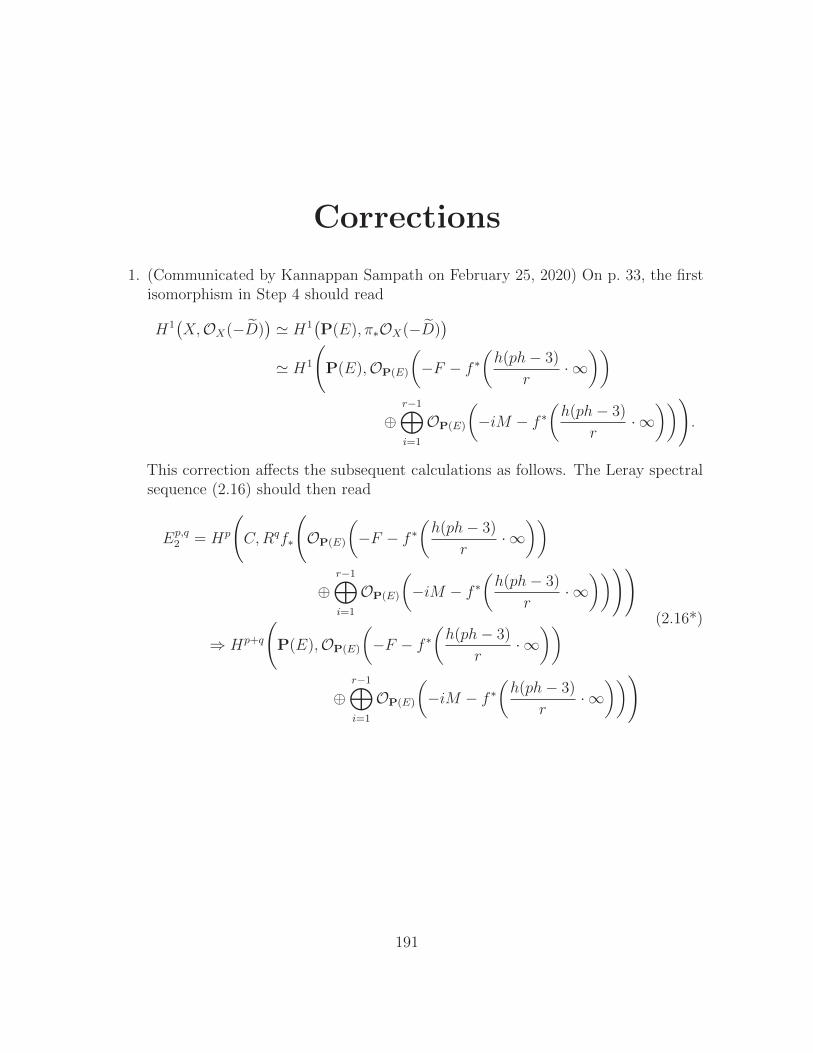
Corrections

1. (Communicated by Kannappan Sampath on February 25, 2020) On p. 33, the firstisomorphism in Step 4 should read

H1(X,OX(−D)

)' H1

(P(E), π∗OX(−D)

)

' H1

(P(E),OP(E)

(−F − f ∗

(h(ph− 3)

r· ∞))

⊕r−1⊕

i=1

OP(E)

(−iM − f ∗

(h(ph− 3)

r· ∞)))

.

This correction affects the subsequent calculations as follows. The Leray spectralsequence (2.16) should then read

Ep,q2 = Hp

(C,Rqf∗

(OP(E)

(−F − f ∗

(h(ph− 3)

r· ∞))

⊕r−1⊕

i=1

OP(E)

(−iM − f ∗

(h(ph− 3)

r· ∞))))

⇒ Hp+q

(P(E),OP(E)

(−F − f ∗

(h(ph− 3)

r· ∞))

⊕r−1⊕

i=1

OP(E)

(−iM − f ∗

(h(ph− 3)

r· ∞)))

(2.16*)

191

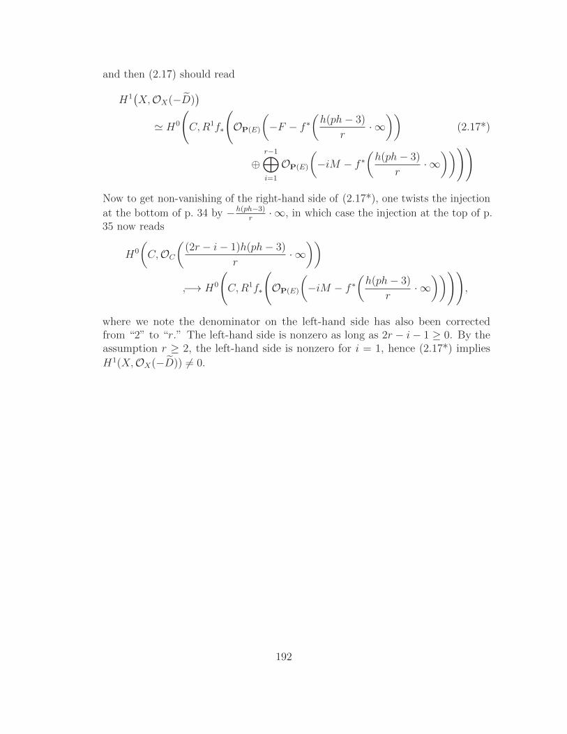
and then (2.17) should read

H1(X,OX(−D)

)

' H0

(C,R1f∗

(OP(E)

(−F − f ∗

(h(ph− 3)

r· ∞))

(2.17*)

⊕r−1⊕

i=1

OP(E)

(−iM − f ∗

(h(ph− 3)

r· ∞))))

Now to get non-vanishing of the right-hand side of (2.17*), one twists the injection

at the bottom of p. 34 by −h(ph−3)r· ∞, in which case the injection at the top of p.

35 now reads

H0

(C,OC

((2r − i− 1)h(ph− 3)

r· ∞))

−→ H0

(C,R1f∗

(OP(E)

(−iM − f ∗

(h(ph− 3)

r· ∞))))

,

where we note the denominator on the left-hand side has also been correctedfrom “2” to “r.” The left-hand side is nonzero as long as 2r − i− 1 ≥ 0. By theassumption r ≥ 2, the left-hand side is nonzero for i = 1, hence (2.17*) implies

H1(X,OX(−D)) 6= 0.

192