Positioning Based on GPS Pseudoranges - The Danish GPS Center

Positioning Based on GPS Pseudoranges

Kai Borre

Aalborg University, Denmark

Location Technology Tutorial June 9, 2001 Espoo

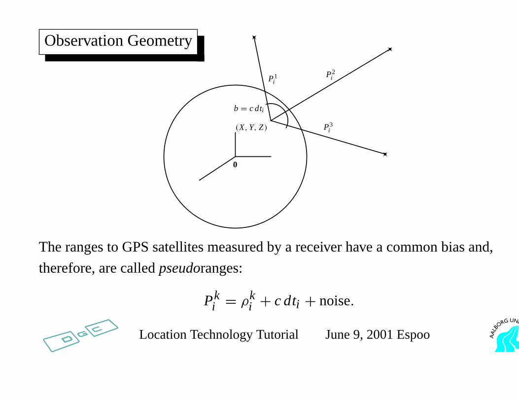
Observation Geometry

0

(X,Y, Z)

P1i

P2i

P3i

b = cdti

××

×

The ranges to GPS satellites measured by a receiver have a common bias and,

therefore, are calledpseudoranges:

Pki = ρk

i + c dti + noise.


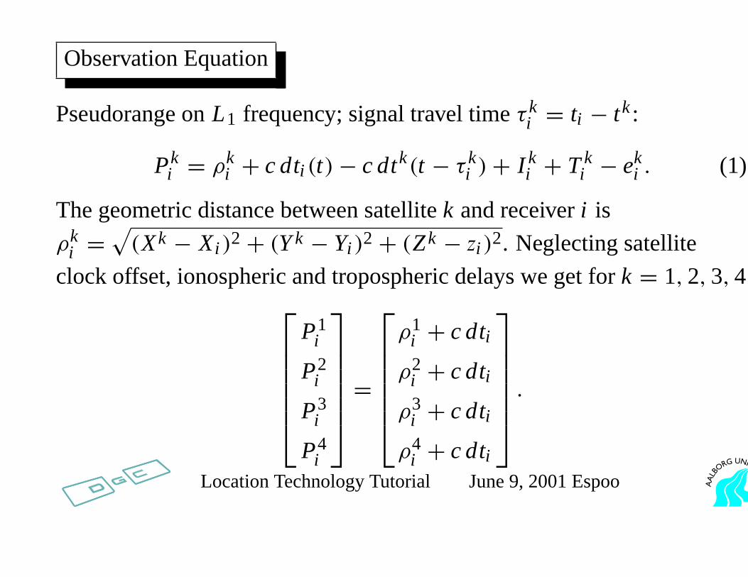
Observation Equation

Pseudorange onL1 frequency; signal travel timeτ ki = ti − tk:

Pki = ρk

i + c dti (t)− c dtk(t − τ ki )+ I k

i + Tki − ek

i . (1)

The geometric distance between satellitek and receiveri is

ρki =

√(Xk − Xi )2+ (Yk − Yi )2+ (Zk − zi )2. Neglecting satellite

clock offset, ionospheric and tropospheric delays we get fork = 1, 2, 3,4

P1i

P2i

P3i

P4i

=

ρ1i + c dti

ρ2i + c dti

ρ3i + c dti

ρ4i + c dti

.


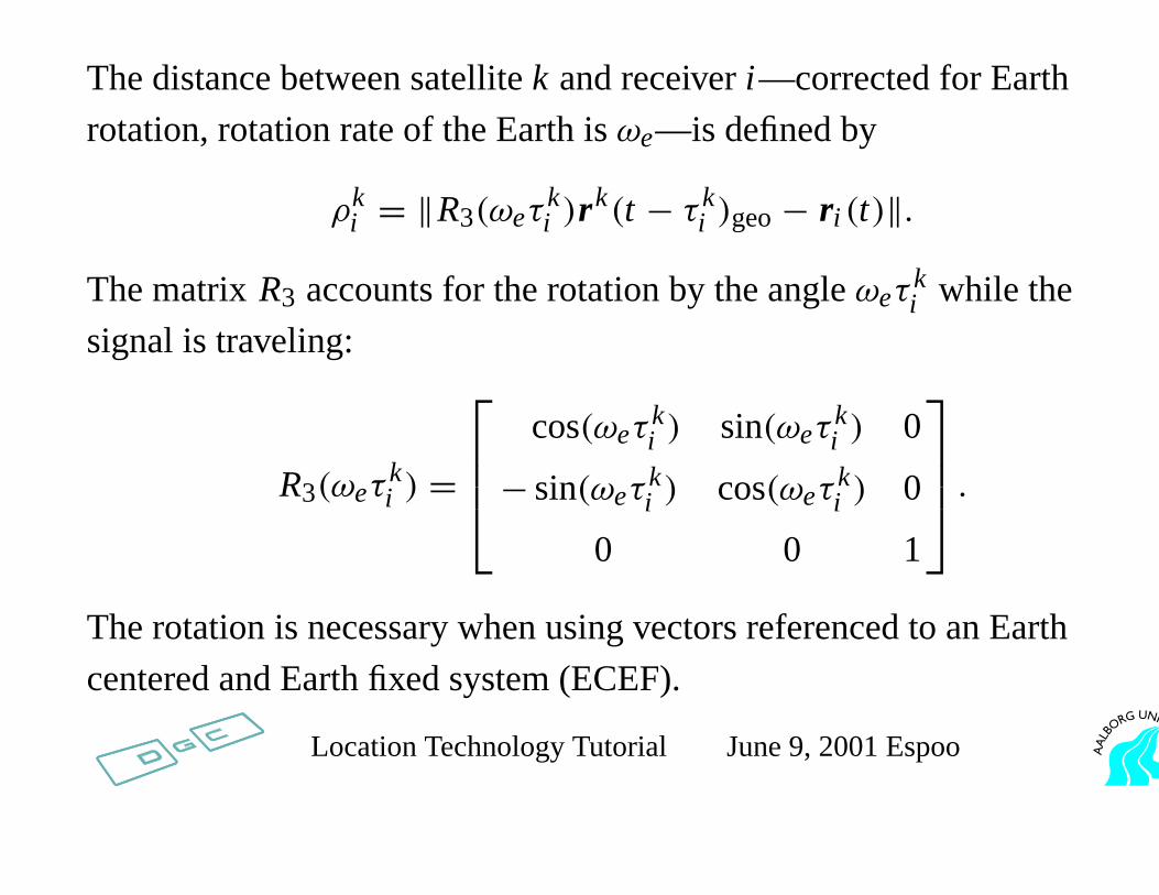
The distance between satellitek and receiveri —corrected for Earth

rotation, rotation rate of the Earth isωe—is defined by

ρki = ‖R3(ωeτ

ki )r

k(t − τ ki )geo− ri (t)‖.

The matrixR3 accounts for the rotation by the angleωeτki while the

signal is traveling:

R3(ωeτki ) =

cos(ωeτki ) sin(ωeτ

ki ) 0

− sin(ωeτki ) cos(ωeτ

ki ) 0

0 0 1

.

The rotation is necessary when using vectors referenced to an Earth

centered and Earth fixed system (ECEF).


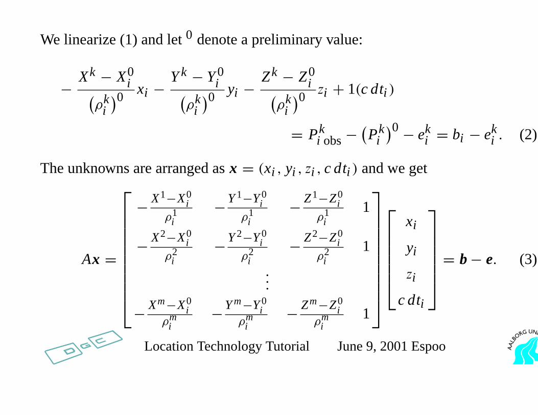
We linearize (1) and let0 denote a preliminary value:

− Xk − X0i(

ρki

)0 xi −Yk − Y0

i(ρk

i

)0 yi −Zk − Z0

i(ρk

i

)0 zi + 1(c dti )

= Pki obs−

(Pk

i)0− ek

i = bi − eki . (2)

The unknowns are arranged asx = (xi , yi , zi , c dti ) and we get

Ax =

− X1−X0i

ρ1i

−Y1−Y0i

ρ1i

− Z1−Z0i

ρ1i

1

− X2−X0i

ρ2i

−Y2−Y0i

ρ2i

− Z2−Z0i

ρ2i

1

...

− Xm−X0i

ρmi

−Ym−Y0i

ρmi

− Zm−Z0i

ρmi

1

xi

yi

zi

c dti

= b− e. (3)


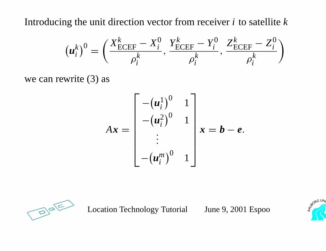
Introducing the unit direction vector from receiveri to satellitek

(uk

i

)0 =(

XkECEF− X0

i

ρki

,Yk

ECEF− Y0i

ρki

,Zk

ECEF− Z0i

ρki

)

we can rewrite (3) as

Ax =

−(u1i

)0 1

−(u2i

)0 1...

−(umi

)0 1

x = b− e.


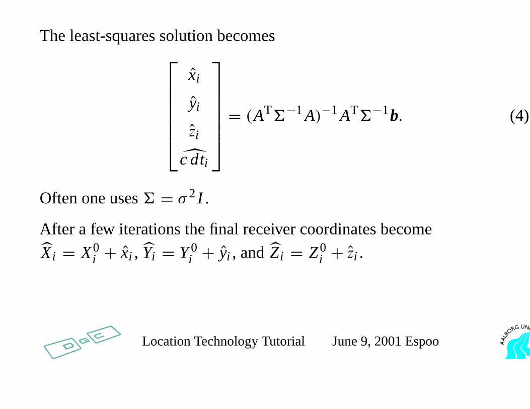
The least-squares solution becomes

xi

yi

zi

c dti

= (AT6−1A)−1AT6−1b. (4)

Often one uses6 = σ 2I .

After a few iterations the final receiver coordinates become

Xi = X0i + xi , Yi = Y0

i + yi , andZi = Z0i + zi .


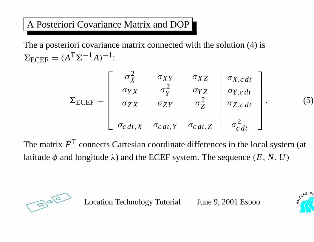
A Posteriori Covariance Matrix and DOP

The a posteriori covariance matrix connected with the solution (4) is

6ECEF= (AT6−1A)−1:

6ECEF=

σ2X σXY σX Z

σY X σ2Y σY Z

σZ X σZY σ2Z

σX,c dt

σY,c dt

σZ,c dt

σc dt,X σc dt,Y σc dt,Z σ2c dt

. (5)

The matrixFT connects Cartesian coordinate differences in the local system (at

latitudeφ and longitudeλ) and the ECEF system. The sequence(E, N,U )


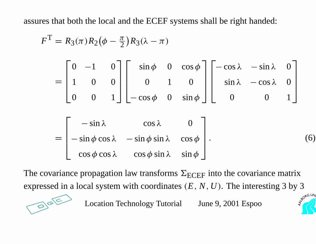
assures that both the local and the ECEF systems shall be right handed:

FT = R3(π)R2(φ − π

2

)R3(λ− π)

=

0 −1 0

1 0 0

0 0 1

sinφ 0 cosφ

0 1 0

− cosφ 0 sinφ

− cosλ − sinλ 0

sinλ − cosλ 0

0 0 1

=

− sinλ cosλ 0

− sinφ cosλ − sinφ sinλ cosφ

cosφ cosλ cosφ sinλ sinφ

. (6)

The covariance propagation law transforms6ECEF into the covariance matrix

expressed in a local system with coordinates(E, N,U ). The interesting 3 by 3


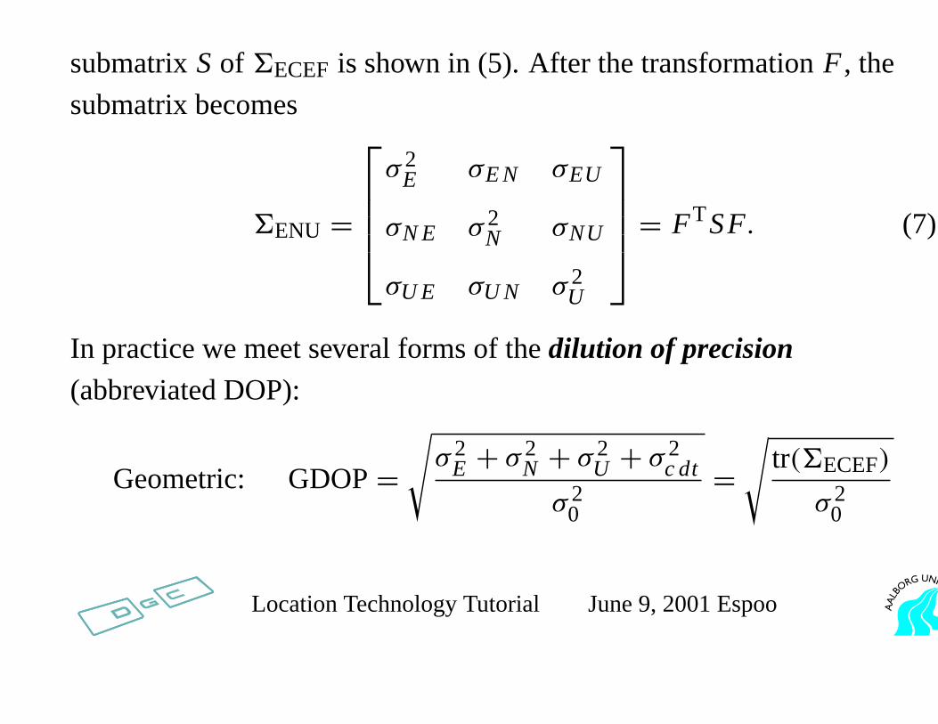
submatrixSof 6ECEF is shown in (5). After the transformationF , the

submatrix becomes

6ENU =

σ 2E σE N σEU

σN E σ 2N σNU

σU E σU N σ 2U

= FTSF. (7)

In practice we meet several forms of thedilution of precision(abbreviated DOP):

Geometric: GDOP=√σ 2

E + σ 2N + σ 2

U + σ 2c dt

σ 20

=√

tr(6ECEF)

σ 20


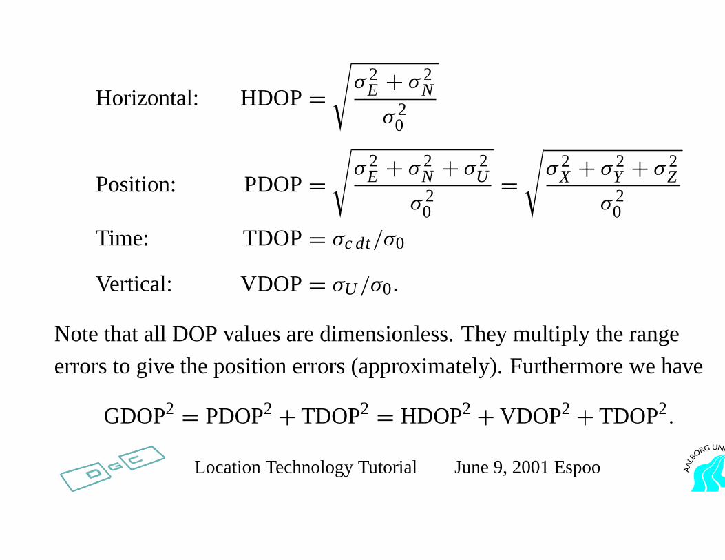
Horizontal: HDOP=√σ 2

E + σ 2N

σ 20

Position: PDOP=√σ 2

E + σ 2N + σ 2

U

σ 20

=√σ 2

X + σ 2Y + σ 2

Z

σ 20

Time: TDOP= σc dt/σ0

Vertical: VDOP= σU/σ0.

Note that all DOP values are dimensionless. They multiply the range

errors to give the position errors (approximately). Furthermore we have

GDOP2 = PDOP2+ TDOP2 = HDOP2+ VDOP2+ TDOP2.


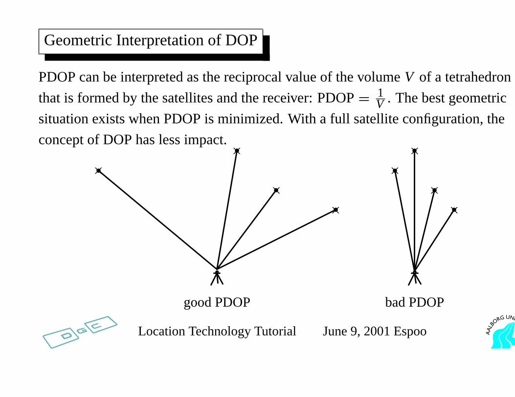
Geometric Interpretation of DOP

PDOP can be interpreted as the reciprocal value of the volumeV of a tetrahedron

that is formed by the satellites and the receiver: PDOP= 1V . The best geometric

situation exists when PDOP is minimized. With a full satellite configuration, the

concept of DOP has less impact.

××

××

goodPDOP

××

××

badPDOP


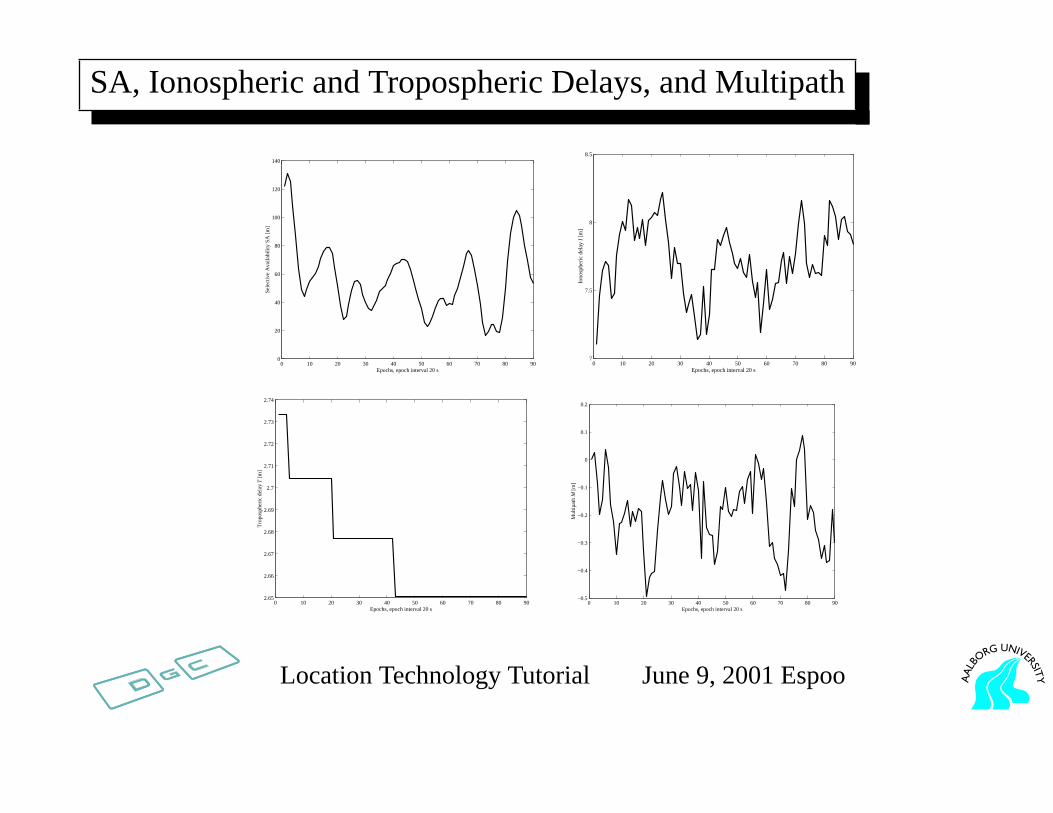
SA, Ionospheric and Tropospheric Delays, and Multipath

0 10 20 30 40 50 60 70 80 900

20

40

60

80

100

120

140

Epochs, epoch interval 20 s

Sele

ctiv

e A

vaila

bilit

y SA

[m

]

0 10 20 30 40 50 60 70 80 907

7.5

8

8.5


Iono

sphe

ric

dela

y I

[m]

0 10 20 30 40 50 60 70 80 902.65

2.66

2.67

2.68

2.69

2.7

2.71

2.72

2.73

2.74


Tro

posp

heri

c de

lay

T [m

]

0 10 20 30 40 50 60 70 80 90−0.5

−0.4

−0.3

−0.2

−0.1

0

0.1

0.2


Mul

tipat

h M

[m

]


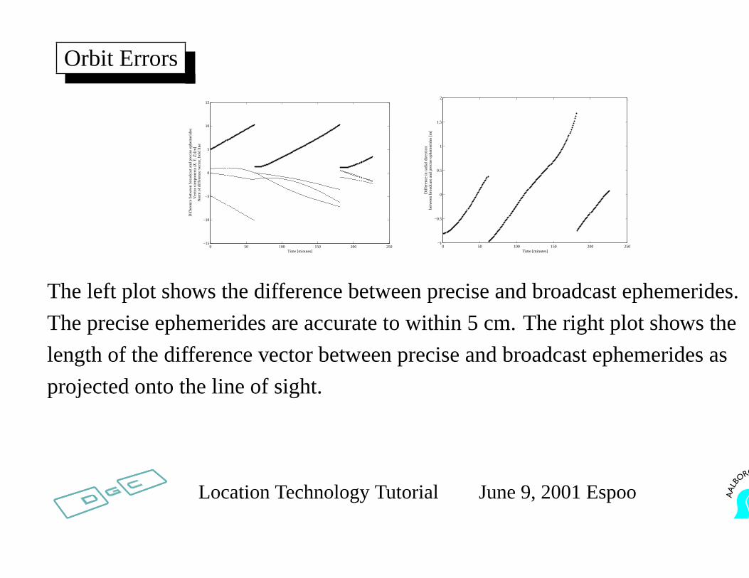
Orbit Errors

0 50 100 150 200 250−15

−10

−5

0

5

10

15

Time [minutes]

Diff

eren

ce b

etw

een

broa

dcas

t and

pre

cise

eph

emer

ides

Vec

tor

com

pone

nts

(X

, Y, Z

) [m

]N

orm

of

diff

eren

ce v

ecto

r, b

old

line

0 50 100 150 200 250−1

−0.5

0

0.5

1

1.5

2

Time [minutes]

Diff

eren

ce in

rad

ial d

irect

ion

betw

een

broa

dcas

t and

pre

cise

eph

emer

ides

[m]

The left plot shows the difference between precise and broadcast ephemerides.

The precise ephemerides are accurate to within 5 cm. The right plot shows the

length of the difference vector between precise and broadcast ephemerides as

projected onto the line of sight.


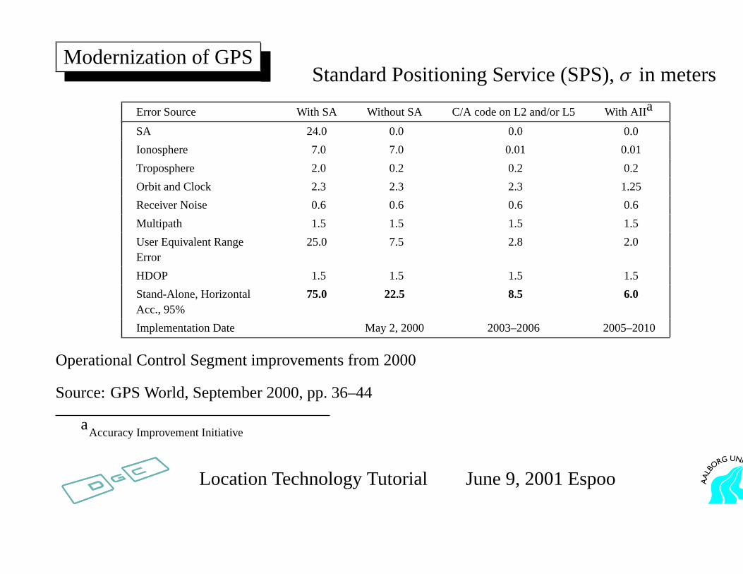
Modernization of GPSStandard Positioning Service (SPS),σ in meters

Error Source With SA Without SA C/A code on L2 and/or L5 With AIIa

SA 24.0 0.0 0.0 0.0

Ionosphere 7.0 7.0 0.01 0.01

Troposphere 2.0 0.2 0.2 0.2

Orbit and Clock 2.3 2.3 2.3 1.25

Receiver Noise 0.6 0.6 0.6 0.6

Multipath 1.5 1.5 1.5 1.5

User Equivalent RangeError

25.0 7.5 2.8 2.0

HDOP 1.5 1.5 1.5 1.5

Stand-Alone, HorizontalAcc., 95%

75.0 22.5 8.5 6.0

Implementation Date May 2, 2000 2003–2006 2005–2010

Operational Control Segment improvements from 2000

Source: GPS World, September 2000, pp. 36–44

aAccuracy Improvement Initiative


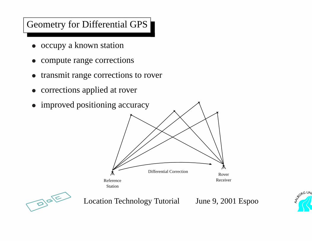
Geometry for Differential GPS

• occupy a known station

• compute range corrections

• transmit range corrections to rover

• corrections applied at rover

• improved positioning accuracy

ReferenceStation

RoverReceiver

DifferentialCorrection

××

×

×


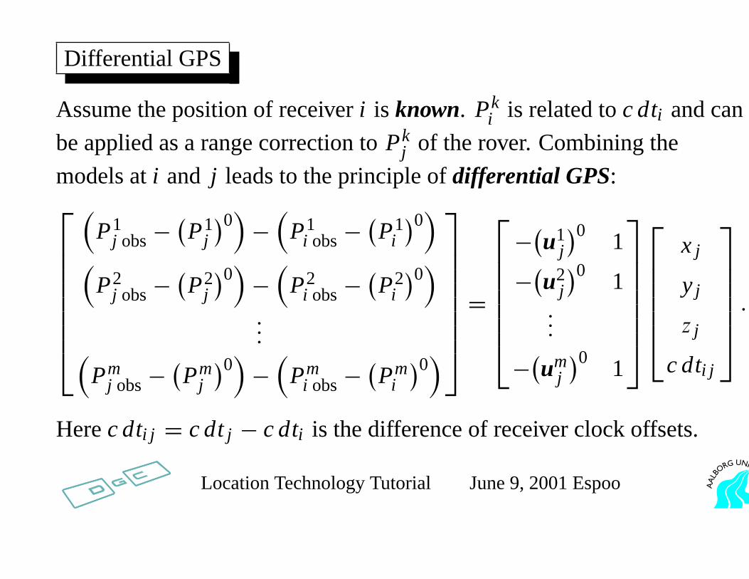
Differential GPS

Assume the position of receiveri is known. Pki is related toc dti and can

be applied as a range correction toPkj of the rover. Combining the

models ati and j leads to the principle ofdifferential GPS:

(P1

j obs−(P1

j

)0)−(

P1i obs−

(P1

i

)0)

(P2

j obs−(P2

j

)0)−(

P2i obs−

(P2

i

)0)

...(Pm

j obs−(Pm

j

)0)−(

Pmi obs−

(Pm

i

)0)

=

−(u1j

)0 1

−(u2j

)0 1...

−(umj

)0 1

x j

y j

z j

c dti j

.

Herec dti j = c dtj − c dti is the difference of receiver clock offsets.


Wide Area DGPS (WADGSP)

WADGPS provides a powerful means for bridging the gap between single site and

high-accuracy positioning in the vicinity of a correction station:

1. Monitor stations at known locations collect GPS pseudoranges from all

satellites in view

2. Pseudoranges and dual-frequency ionospehric delay measurements (if

available) are sent to the master station

3. Master station computes an error correction vector

4. Error correction vector is transmitted to users

5. Users apply error corrections to their measured pseudoranges and collected

ephemeris data to improve navigation accuracy.


Internet-based Global DGPS

NASA’s Global GPS Network (GGN) is operated and maintained by JPL.

GGN consists of more then 60 sites in batch mode over the Internet

igscb.jpl.nasa.gov. Software used:

• Real-Time Net Transfer (RTNT)

• Real-Time GIPSY (RTG).

The open Internet is a reliable choice to return GPS data for a state-space

global differential system. User positions accurate to sub-meter level.

gipsy.jpl.nasa.gov/igdg/system/index.html


Virtual Reference Station

Data from several reference stations are collected and processed in

real-time using standard software.

Via the Internet the user asks for data from a non-exisiting reference

station at a user specified location. The accuracy is comparable to the one

obtained from a rigorous network solution.

Source: H. van der Marel (1998)Virtual GPS Reference Stations in the Netherlands.

ION GPS-98, pp. 49–58


GPS for Precise Time

GPS is the primary system for distribution of Precise Time and Time Interval

(PTTI). The time scales are

• time kept by a satellite clocktk

• GPS timetGPSdefined by the Control Segment on the basis of a set of

atomic standards aboard the satellites and in monitor stations

• UTC (USNO)tUTC the US national standard defined by the US Naval

Observatory

• time kept by a user’s receiver clockti

δtUTC = tGPS− tUTC is currently estimated to be about 10 ns.

Synchronization of clocks by common-view mode.


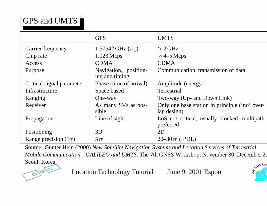
GPS and UMTS

GPS UMTS

Carrier frequency 1.57542 GHz (L1) ≈ 2 GHzChip rate 1.023 Mcps ≈ 4–5 McpsAccess CDMA CDMAPurpose Navigation, position-

ing and timingCommunication, transmission of data

Critical signal parameter Phase (time of arrival) Amplitude (energy)Infrastructure Space based TerrestrialRanging One-way Two-way (Up- and Down Link)Receiver As many SVs as pos-

sibleOnly one base station in principle (’no’ over-lap design)

Propagation Line of sight LoS not critical, usually blocked, multipathpreferred

Positioning 3D 2DRange precision (1σ ) 5 m 20–30 m (IPDL)

Source: Gunter Hein (2000)New Satellite Navigation Systems and Location Services of TerrestrialMobile Communication—GALILEO and UMTS. The 7th GNSS Workshop, November 30–December 2,Seoul, Korea.


Recommended Literature

Enge, P. & P. Misra (ed.s) (1999)Proceedings of the IEEE, 87: 3–172

Strang, Gilbert & Kai Borre (1997)Linear Algebra, Geodesy, and GPS.

Wellesley-Cambridge Press

Kaplan, E. D. (ed.) (1996)Understanding GPS Principles and

Applications. Artech House

Misra, Pratap & Per Enge (2001)Global Positioning System. Signals,

Measurements, and Performance. Ganga-Jamuna Press, in preparation


Samples of Useful Links on the Internet

GPS in General

www.navcen.uscg.mil

GPS New Signal Structure

www.ima.umn.edu/talks/workshops/8-16-18.2000

GPS Matlab files

kom.auc.dk/˜borre/matlab

OEM boards

www.sirf.com

www.motorola.com/ies/GPS/products/gpsprod.html

www.topconps.com

GPS fleet management

www.thales-navigation.com


Galileo about to Move Ahead

Galileo in general

www.galileo-pgm.org

Galileo newsletters

www.genesis-office.org

EU information about Galileo

europa.eu.int/comm/energy transport/en/gal en.html

Source: Christian Tiberius & Peter Joosten (2001)Galileo about to Move Ahead. GIM International,

March 2001, pp. 14–17.


Positioning Based on GPS Pseudoranges - The Danish GPS Center

Documents

Transcript of Positioning Based on GPS Pseudoranges - The Danish GPS Center